Published by 1. Ali N. Hamoodi1, 2. Waseem Kh. Ibrahim2, 3. Aseel Thamer Ebrahem3, Northern Technical University (1), Northern Technical University (2), Northern Technical University (3) ORCID: 1. 0000-0003-0991-3538; 2. 0000-0002-9126-7872; 3. 0000-0002-1090-0454
Abstract. A photovoltaic (PV) is a technical terminology that is used to generate electricity from sunlight. Solar energy is one of the solutions for solving the electricity needs in any area. Designing a grid-tie PV system based on real data is very important to utilize a great system. The case study was taken on a national thermal power corporation (NTPC) that lies at Gomti Nager in India. In this work, Newzealand mathematical calculation method is used to design a PV system and a comparison between conventional PV systems and nano PV systems is made. It has been concluded that the nano-PV system cost was lesser than the conventional PV system.
Streszczenie. Fotowoltaika (PV) to terminologia techniczna używana do wytwarzania energii elektrycznej ze światła słonecznego. Energia słoneczna jest jednym z rozwiązań pozwalających na zaspokojenie zapotrzebowania na energię elektryczną w dowolnym obszarze. Projektowanie sieciowego systemu fotowoltaicznego opartego na rzeczywistych danych jest bardzo ważne, aby wykorzystać świetny system. Studium przypadku dotyczyło krajowej korporacji energetycznej (NTPC), która znajduje się w Gomti Nager w Indiach. W tej pracy do zaprojektowania systemu fotowoltaicznego zastosowano matematyczną metodę obliczeń Newzealand i dokonano porównania między konwencjonalnymi systemami fotowoltaicznymi a nano systemami fotowoltaicznymi. Stwierdzono, że koszt systemu nano-PV był niższy niż w przypadku konwencjonalnego systemu PV. (Projekt systemu zasilania fotowoltaicznego: przypadek między dwoma różnymi typami modułów słonecznych)
Keywords: photovoltaic system, PV system design, conventional PV system, nano PV system, grid-tie. Słowa kluczowe: system fotowoltaiczny, nano PV system
Introduction
Generating electricity with consuming classical infinitives is steered to the evolution of (PV) systems [1]. These PV systems depended on sunlight for generating electricity. The efficiency of the traditional PV modules is lower than that of nano modules [2], [3]. In order to design a solar energy plant, some real conditions must be available: solar radiation, load profile, solar energy potential, and installation areas are needed; energy consumption amount in these areas represents the main factor in the design, also the load growth discretion is requested in order to enable the installed system works with good manner. These researcher projections are used for designing a solar system. The number of batteries and capacities used in the remote areas must have a little wasted energy. The fixture for declining cost of electric power and reliability in isolated regions in the world is the essential force driving the worldwide PV industry during the present time. Exemplary applications of PV that use today involve grid-tie PV systems for remote and cottages residences [4].
System Components
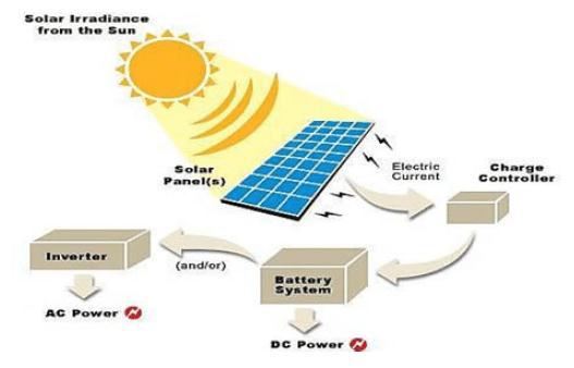
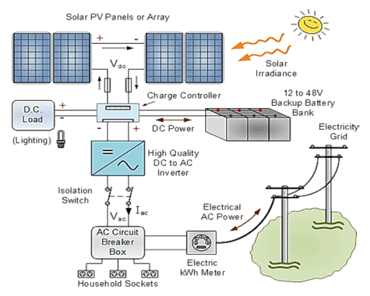
The functional and working needs designate components, which are included within the PV system [5]. The main components of the PV system as illustrated in Fig.1 are PV modules, MPPT-controller inverter, battery bank, and loads.
Fig.1 PV system components
PV modules:
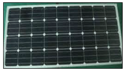
Fig.2. represents the picture of the SunPower 220W PV module.
Fig.2 SunPower 220W PV module
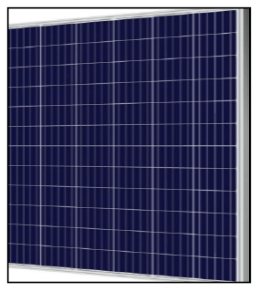
Fig.3 Renesola 220W PV module
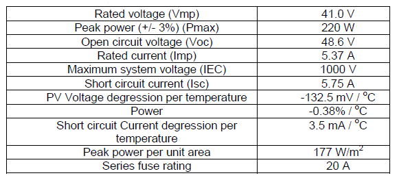
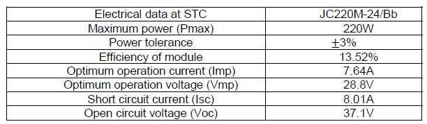
The specifications of SunPower 220W PV module are given in table1.
Table1. SunPower 220W PV module parameters.
.
Electrical Data Measured under Standard Test Conditions (STC): Irradiance of 1000/m2, cell mass, and air temperature 25oC.
Fig.3. represents the picture of Renesola 220W PV module 156 series polycrystalline solar module. The specifications of Renesola 220W PV module are given in table2.
Table 2. Renesola 220W PV module parameters.
.
Values under standard test conditions STC (Irradiance 1000W/m2, Cell temperature 25oC, Air mass 1.5).
Battery type
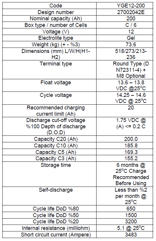
The battery type that used in this storage system is a 12V, 200Ah gel VRLA deep cycle. Fig. 4 represents the battery shape and its specifications are illustrated in table 3 [7]. Gel battery shows some discriminatory advantages, such as good recovery from deep discharge, high deep discharge capability, and super thermal stability even if this type of batteries are left discharged for 3 days, they will recover to 100% of capacity.
Table 3. Battery specifications
.
Inverter type
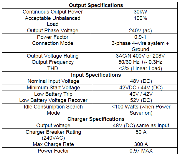
The inverter type that used is in this PV system is a 30kW model, in order to control DC to AC and connected with the grid (grid-tie).
The specifications of 30kW grid-tie three-phase inverter is given in table4.
Table 4. Three phase gird-tie 30kW inverter specifications
.
Array inclination
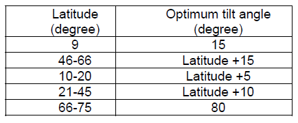
The position of PV modules usually facing the north in the southern hemisphere and the south in the northern hemisphere. Therefore, PV modules are fixed semper faces the sun at noon. In winter, an acuter angle tilting will increase the output while in summer the smaller angle will give more output.
Table 5. Illustrates the optimum tilt angle at different latitude.
Table 5. Tilt angle of PV module
.
Designing and calculation of PV system (case study)
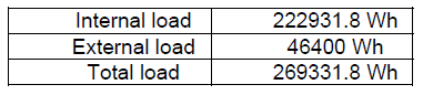
(NTPC) is a famous organization in the northern region of the country (India). The building called (NRHQ) of NTPC organization lie at Gomti Nagar. The total load of this building is given in table 6.
Table 6. Load of building
.
Flowchart and Methodology
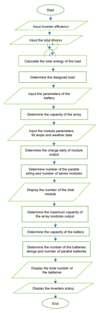
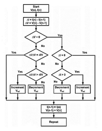
The mathematical procedures that used to design the solar PV system based Newzealand method is shown in Fig. 4.
Mathematical concept of solar PV system
In order to evaluate solar PV system, Newzealand design method has been used, a quick guide is used to calculate the total energy of any building, number of PV modules, number of batteries and inverter capacity. Solar PV systems come in a diversity of factors and a range of electricity generating capacities. At the first stage, the amount of total power that typically use and the number of hours of sunlight per day according to the location must be determined [9-17].
Fig.4 Flowchart of solar PV system design based on Newzealand method
A- Conventional SunPower 200W PV module
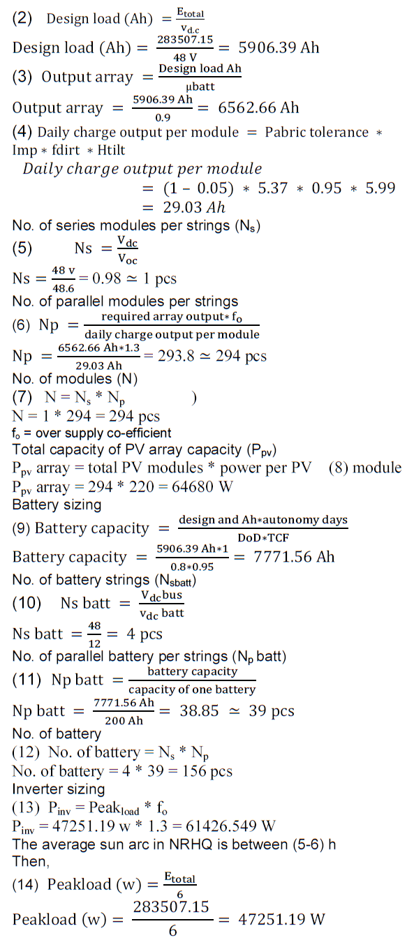
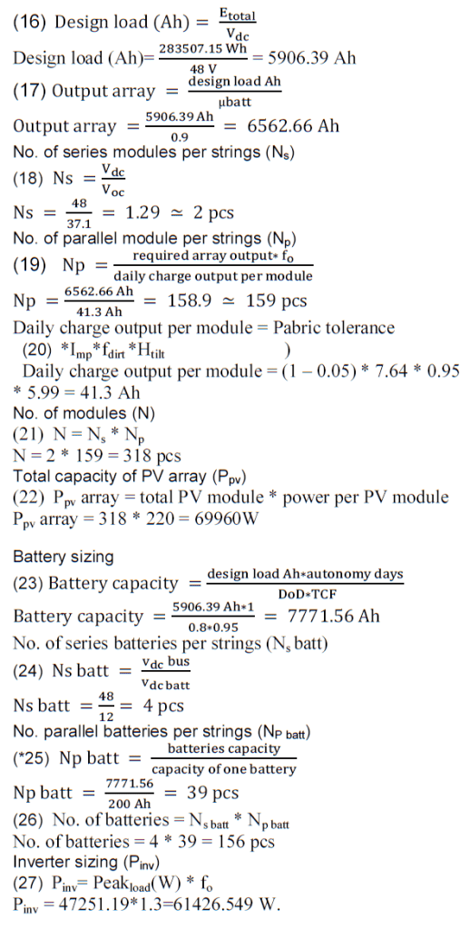
PV sizing
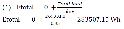
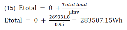
Design load energy (Etotal)
.
.
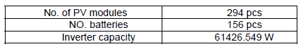
The elements of conventional PV system can be summarized as given in table 7.
Table7. Components of conventional PV system
.
B- Renesola polycrystalline solar module nano PV module (220W)
PV sizing
Design load energy (Etotal)
.
.
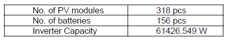
The elements of nano PV system can be summarized as given in table 8.
Table8. Components of Nano PV system
.
Conclusions
From the results, the number of nano PV modules are more than that the conventional PV modules, same batteries and inverter capacity for same grid-tie PV systems, Nano technology give mire efficiency working performance and low cost for same PV module power. The total cost for designing grid-tie nano PV system is more economical than that of conventional PV system due to less number of the battery bank, in spite of the increase number in PV modules but the batteries number have significant affect on the total cost. When the dirt factor and H tilt angle increases the number of parallel modules per string decrease. The capacity of the battery increases as the DoD decrease.
REFERENCES
1. M.N.Bandyopadhyay & O.P.Rahi, ”Non-Conventional Energy Sources”, Proceedings of All India Seminar on Power Systems: Recent Advances and Prospects in 21st Centure, AICTE, Jaipur, 17 February 2001, pp 1-3. 2. A. Dey, A. Tripathi, A Verma & A. Bandha, ”Analysis of Solar Photovoltaic (SPV) Systems for Residential Applicating”, National Journal of the IE(I), Vol. 87, May 06, pp 6-9. 3. Tracy Dahl, ”Photovoltaic Power Systems Technology”, White paper, http://www.polarpower.org, 2004, pp 1-33. 4. Angga Romana, Eko Adhi Setiawan & Icurnianto Joyonegoro, ”Comparison of Two Calculation Methods for Designing the Solar Electric Power System for Small Island”, E35 Web of Conference 67,02052 (2018), 3rd i-TREC 2018, pp 1-6. 5. http://www.sma.de/en/solutions/meduim-power-solutions/smasmart-home.html. 6. http://www.solarguru.com.au/PDFs/NG12-200.pdf. 7. https://www.yigitaku.com/wp-content/uploads/2018/07/12V-200Ah-Jel-Eng.pdf. 8. https://www.serveafri.com/products/60kw-solar-grid-tie-inverterthree-phase. 9. https://www.motherearthnews.com/renewable-energy/solarpower-systems-zmaz98onzraw. 10. Sarat Kumar Sahoo “Renewable and sustainable energy reviews solar photovoltaic energy progress in India: A review “, http://www.elsevier.com/locate/rser, Renewable and Sustainable Energy Reviews 59 (2016) 927–939. 11. Rupendra Pachauri, Om Prakash Mahela, Abhishek Sharma, Jianbo Bai, Yogesh K. Chauhan, Baseem Khan &Hassan Haes Alhelou, “Impact of Partial Shading on Various PV Array Configurations and Different Modeling Approaches: A Comprehensive Review”, DOI 10.1109/ACCESS.2020.3028473, IEEE Access. 12. Mohammed Yaqoot, Parag Diwan, Tara C. Kandpal, “Financial attractiveness of decentralized renewable energy systems – A case of the central Himalayan state of Uttarakhand in India”, Renewable Energy 101 (2017) 973e991. 13. Hamoodi SA, Hameed FI, Hamoodi AN. Pitch angle control of wind turbine using adaptive Fuzzy-PID controller. Mosul, Iraq: Northern Technical University (NTU), Engineering Technical College, EAI endorsed transactions on energy web; 2020 Jul.7. p. 1–8. 14. 14. Hamoodi SA, Hamoodi AN, Haydar GM. Automated Irrig Syst based soil moisture using arduino board. Bulletin of electrical engineering and informatics. Iraq: Northern Technical University (NTU), Engineering Technical College; 2020 June 3.p. 870–6. 15. Hamoodi AN, Hamoodi SA, Mohammed RA. Photovoltaic modeling and effecting of temperature and irradiation on I– Vand P–V characteristics. Northern Technical University (NTU),Engineering Technical College, Iraq. Int J Appl Eng Res India Publ. 2018;13(5):3123–7. http://www.ripublication.com. 16. Hamoodi AN, Hamoodi SA, Ibrahim MA. “Power factor correction of AC to DC converter using boost chopper.” Northern Technical University (NTU), Engineering Technical College, Iraq. J Eng Appl Sci. 2018;13(Special Issue 8):6440– 5. 17. Hamoodi AN, Hamoodi SA, Abdulla AG. “Photovoltaic-battery system tested under sun irradiance”. Northern Technical University (NTU), Engineering Technical College, Iraq. Lond J Eng Res. 2018;18(2):65–75.
Authors. Dr. Ali Nathim Hamoodi Northern Technical University (NTU)/Technical College of Engineering, Mosul-Iraq. Email: ali_n_hamoodi74@ntu.edu.iq. Waseem Khalid Ibrahim Northern Technical University (NTU)/Technical College of Engineering, Mosul-Iraq. Email: waseem_kh82@ntu.edu.iq. Aseel Thamer Ebrahem obtained her B.Sc. (2004) and M.Sc. (2014) in Computer Engineering Technology from Northern Technical University (NTU). Currently, she is working as assistant lecturer in Computer Engineering department, in Northern Technical University (NTU)/ Technical College of Engineering, Mosul-Iraq. Email: aseelthamer@ntu.edu.iq.
Source & Publisher Item Identifier: PRZEGLĄD ELEKTROTECHNICZNY, ISSN 0033-2097, R. 99 NR 2/2023. doi:10.15199/48.2023.02.65
Published by Małgorzata ZYGARLICKA1, Jarosław ZYGARLICKI2, Politechnika Opolska, Instytut Automatyki i Informatyki (1) Politechnika Opolska, Instytut Elektroenergetyki i Energii Odnawialnej (2)
Abstract. The paper presents a new proposal for the presentation of the harmonic distortion of the power signals. The proposed method uses a simplified method of harmonic analysis – five ordinates method by which a transient characteristics of the power grid is represented. The article presents sample analysis of real-life power signals.
Streszczenie. Artykuł przedstawia nową propozycję prezentacji zniekształceń harmonicznych dla sygnałów elektroenergetycznych. Proponowany sposób wykorzystuje uproszczoną metodę analizy harmonicznych – metodę pięciu rzędnych, dzięki której odtwarzana jest charakterystyka przejściowa układu czwórnika reprezentującego badaną sieć elektroenergetyczną. W artykule zmieszczono przykładowe analizy rzeczywistych sygnałów elektroenergetycznych. (Sposób prezentacji zniekształceń harmonicznych sygnałów elektroenergetycznych).
Keywords: power quality, signal analysis, signal processing, harmonics Słowa kluczowe: jakość energii elektrycznej, analiza sygnałów, przetwarzanie sygnałów, harmoniczne
Introduction
Harmonic distortion of electrical signal is one of the basic parameters to describe the quality of electric energy. An analysis of harmonic distortion levels enables to specify the causes of states that occur in the power supply network and cause malfunction of connected appliances. Harmonic distortion in the power grid is caused by appliances with non-linear characteristics of power consumption. The proposed method of presenting harmonic distortion enables to identify the sources of distortion by observing transient characteristics, as reconstructed on the basis of the harmonic distortion, of the four-pole system representing power grid together with appliances connected to it.
This article has been divided into 5 main sections. The first section is an introduction to the subject of this paper. The second section describes the proposed method of presenting the harmonic distortion. The next section describes the measurement system and method of recording signals subjected to analysis. The fourth section presents the tests and discussion of obtained results. The last section presents the conclusions of this study.
Description of method
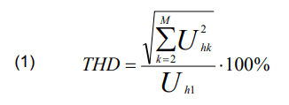
Total Harmonic Distortion (THD) is the most popular factor to quantitatively describe the parameters of the electric energy quality. This factor is defined as the ratio between the amplitude of signal’s higher harmonics and amplitude of the fundamental harmonic component:
.
where: M is the number of harmonic components, for which THD is calculated, Uhk it is the amplitude of k-th harmonic component for k = 1, 2, …, M, Uh1 is the amplitude of the fundamental harmonic component. THD measurement, in testing the quality of electric energy, is carried out by means Fourier transform of the electrical signal. In diagnosing the state of the power supply network, factors that describe the share of individual harmonics in the analysed signal, are also used.
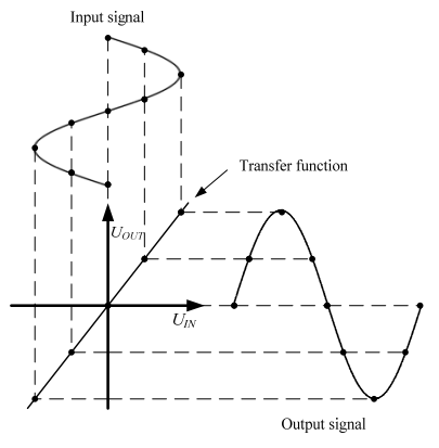
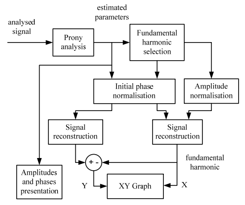
However, it has been found out that analysis of results that describe the levels of harmonics does not directly reveal the causes of harmonics’ generation in electrical wiring systems; thus, the idea to apply the method of five-ordinates [1], [2] to reconstruct the transient characteristics of the four-pole system representing power supply network together with connected appliances causing interference. Schematically, the idea of the proposed method of presenting the harmonic distortion is shown in Figure 1. The input signal is a perfect sinusoid that represents the supply voltage waveforms without harmonic distortion. In reality, the recorded signal – the output signal in Figure 1, is distorted due to the occurrence of non-linear loads in the power supply network. On the basis of the calculated amplitudes and initial phases of individual harmonics, it is possible to reconstruct the transient characteristics of the system presented in this way. The parameters of signals were calculated using Prony’s method [3] – [6]. The shape of this characteristics shows the characteristic points, based on which, it is possible to deduct the causes of harmonics’ formation.
Fig.1. Five ordinates method for determining the coefficient of harmonics
However, the reconstructed characteristics, as obtained in this way, will not clearly reveal the distortion caused by the harmonics, since such distortion has low amplitude in relation to the fundamental component 50 Hz. In order to enhance the clarity of the analysis, in the proposed method of presenting distortion, the values that are a difference between the values of voltages resulting from an ideal transient characteristics and real characteristics are presented on the axis of ordinates. In this way, clarity of phenomena occurring during distortion generation, has been significantly improved.
Measurement system
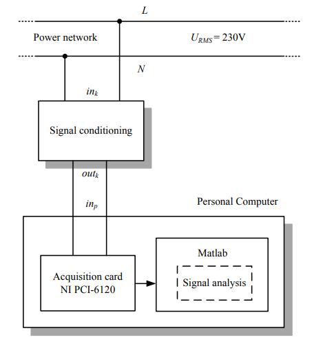
The measurement system, as shown in Figures 2 and 3, has been used in this study. Real signals from the power grid, which are voltage waveforms, are applied at the input of the signal conditioning system. In this system, the amplitude of voltage waveforms is reduced to a level acceptable by the input of the A/C transformer. From the output of the signal conditioning system, the voltage waveforms are applied to the input of the measurement card, in this card they are converted to a digital form, which is processed in the next step in the Matlab computing environment according to the proposed algorithm. Sample signals were recorded with a resolution of 16 bits and a sampling frequency of 12,8 kHz.
Fig.2. The measurement system for acquiring power signal waveforms
Fig.3. Proposed method of power signal waveforms analysis
Tests
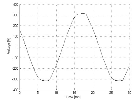
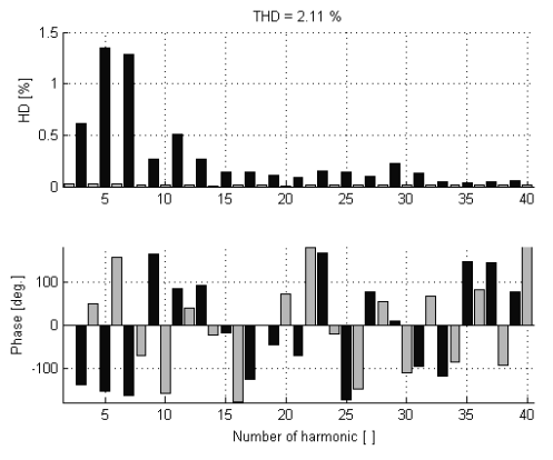
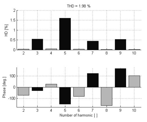
Figures 4-7 show the results for the sample #1 signal recorded in the low voltage network in building II of Opole University of Technology, 76 Prószkowska Street, on 24 January 2016 at 11:26. Figure 4 shows a section of time voltage waveform. Figure 5 illustrates the designated levels of harmonics, their initial phases and THD. Figures 6 and 7 show the proposed method of presenting distortion for 10 and 40 harmonics respectively. “H1 deviation” on Figure 6 and 7 shows overvoltage event of measured fundamental harmonic.
After analysis of Figure 5, the person diagnosing given power supply network, apart from the level of individual harmonics, is not able to determine the nature of the observed distortions. While the method proposed in Figures 6 and 7 reveals that the harmonic distortions appear mainly in areas adjacent to the absolute maximum values of momentary voltage, meaning on the extremes of the transient characteristics. Such an observation suggests that in the given system, the appliances generating interference take current in pulses near the absolute maximum values of voltage waveform. Additionally, a different distortion of characteristics is noticeable for an increasing voltage waveform and a different one for decreasing waveform, which in this case, suggests the source of interference of capacitive nature. Thus, in the presented case, the harmonic distortion is largely generated by the switching power supplies, e.g. computer power supplies.
After comparing Figure 6 and 7, an increase in the detail of diagrams is noticeable, which results from including a larger number of harmonics in creating the transient characteristics. However, it appears, that in this case, the characteristics created already on the basis of the first 10 harmonics make it possible to correctly carry out a diagnosis of sources of interference in the power supply network.
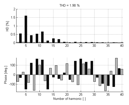
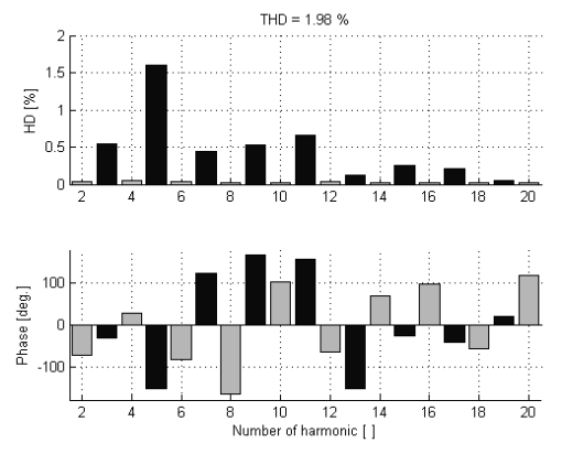
Other results for real life samples of signals recorded in another buildings of Opole University of Technology (signal #2, signal #3 and signal #4) are shown on Figures 8-14.
Fig.4. Segment of voltage waveform of the real life test signal #1
Fig.5. Analysis of harmonics distortion of the signal #1
Fig.6. Transfer function for the test signal #1
Fig.7. Transfer function for the test signal #1
Fig.8. Analysis of harmonics distortion of the signal #2
Fig.9. Transfer function for the test signal #2
Fig.10. Transfer function for the test signal #2
Fig.11. Analysis of harmonics distortion of the signal #3
Fig.12. Transfer function for the test signal #3
Fig.13. Analysis of harmonics distortion of the signal #4
Fig.14. Transfer function for the test signal #4
Conclusions
The proposed new method of presenting harmonic distortion of electrical signals enables to make a more accurate analysis of the phenomena occurring in the power supply networks, as compared to traditional methods based only on an analysis of the harmonic levels. This method enables to determine the causes of harmonics through reconstruction, based on amplitudes and initial phases, of the transient characteristics of four-pole system representing power grid together with connected appliances. In this way, the diagnostics of the power supply network’s states causing failure or malfunction of appliances becomes more reliable and its interpretation more simplified.
REFERENCES
[1] Zygarlicki J., Mroczka J., Method of testing and correcting Signac amplifiers’ transfer function using Prony analysis, Metrology and Measurement Systems (M&S), 19 (2012), nr.3, 489-498 [2] Cykin G., Wzmacniacze sygnałów elektrycznych, WKŁ, Warszawa, 1964 [3] Zygarlicki J., Mroczka J., Prony method used for testing harmonics and interharmonics of electric power signals, Metrology and Measurement Systems (M&S),19 (2012), nr.4, 659-672 [4] Zygarlicki J., Mroczka J., Praktyczne zastosowanie zredukowanej metody Prony’ego – badanie napięciowych układów wejściowych urządzeń monitorujących jakość energii elektrycznej, Przegląd Elektrotechniczny, 5 (2011), 199-203 [5] Rezmer J., Lobos T., Estymacja spektralna zniekształconych sygnałów z zastosowaniem metody Pronego, Przegląd Elektrotechniczny, 10 (2003), 735-738 [6] Hong Li, Zhong Li, Wolfgang A. Halang, Bo Zhang, Guanrong Chen, Analyzing chaotic spectra of DC–DC converters using the Prony method. IEEE Trans. Circuits and Systems-II: Express Briefs, 54 (2007), n.1, 61-65
Autors: dr inż. Małgorzata Zygarlicka, Politechnika Opolska, Instytut Automatyki i Informatyki, ul. Prószkowska 76, 45-758 Opole, E-mail: m.zygarlicka@po.opole.pl; dr hab. inż. Jarosław Zygarlicki, Politechnika Opolska, Instytut Elektroenergetyki i Energii Odnawialnej, ul. Prószkowska 76, 45-758 Opole, E-mail: j.zygarlicki@po.opole.pl
Source & Publisher Item Identifier: PRZEGLĄD ELEKTROTECHNICZNY, ISSN 0033-2097, R. 92 NR 11/2016. doi:10.15199/48.2016.11.18
Published by Wojciech NITA1, Sylwester FILIPIAK2, PGE Dystrybucja S.A. Oddział Skarżysko-Kamienna (1), Politechnika Świętokrzyska (2)
Abstract. This article elaborates on and supplements the research presented in earlier works [19,20,21] on planning for upgrading field MV power grids. While that study developed models for optimizing failure rates (SAIFI, SAIDI, MAIFI) for large areas of the grid, this paper focuses on applying optimization algorithms to more detailed planning for upgrading individual MV lines from the transformer station selected for analysis..
Streszczenie. Niniejszy artykuł zawiera rozwinięcie i uzupełnienie badań przedstawionych we wcześniejszych pracach [19,20,21] dotyczących planowania modernizacji terenowych sieci elektroenergetycznych SN. W tamtych badaniach opracowano modele dla optymalizacji wskaźników awaryjności (SAIFI, SAIDI, MAIFI) dla dużych obszarów sieci, natomiast w niniejszym artykule skupiono się na zastosowaniu algorytmów optymalizacyjnych do bardziej szczegółowego planowania modernizacji poszczególnych linii SN z wybranego do analizy GPZ-tu. (Optymalizacja modernizacji terenowych linii elektroenergetycznych SN z zastosowaniem algorytmów ewolucyjnych).
Słowa kluczowe: sieci elektroenergetyczne, optymalizacja, metody ewolucyjne Keywords: power grids, optimization, evolutionary methods
Introduction
An important issue of the operation of field medium-voltage (MV) distribution power grids is the successive modernization of grid systems to reduce failure rates and improve the efficiency of grid infrastructure [3, 4]. Since power grid systems consist of a very large number of components and use specialized technologies applied to power lines, the problem of planning distribution grid modernization projects is complex.
This article elaborates and complements the research presented in papers [21,22,23] on planning for upgrading field MV power grids. An extension of the optimization models described in the paper [21] is to include criteria for optimizing power distributions and a criterion for optimizing voltage conditions in the analyzed grid, taking into account local conditions including existing or planned to be connected sources of distributed generation (GR).
Earlier works [21,22,23] analyzed large portions of the MV field power distribution grid (the results in the aforementioned works included the analysis of the grid area fed from several transformer stations), in those studies models were developed for optimizing the failure rates (SAIFI, SAIDI, MAIFI) for large areas of the grid, while this article focuses on the application of optimization algorithms for more detailed planning of upgrades of a selected MV line sequentially from the transformer station selected for analysis.
The contribution of new original components to this article involves:
• inclusion in the optimization model of additional criteria for: optimization of power distributions and minimization of voltage deviations at grid nodes,
• implementation of calculations for planning MV line upgrades taking into account distributed generation sources connected or planned to be connected to the line,
• inclusion of structural reliability in computational models and the adaptation of these models to calculations using various reliability indexes,
• development of modifications to the applied evolutionary algorithms (in terms of how solutions are encoded and in terms of recombination operators) for the implementation of calculations for individual MV lines,
• implementation of analysis and determination of the Pareto front for the task of optimizing the planning of MV field line modernization projects.
In Polish and English-language literature on the topic there are published works on the operation of MV distribution grids [2, 30], most often these publications deal with the problems of reconfiguration of distribution grids, among others [16, 17], and the development and expansion of power distribution grids, among others [24, 25, 26], while there are fewer works on the problems of modernization, reconstruction of field MV distribution grids. The need to modernize the country’s field MV power grids is due to various reasons, which include the failure rate of grid equipment resulting from aging processes, as well as the increase in the load on these grids.
Measures that improve the reliability of electric distribution grids can include [14, 20, 21, 31, 32]:
• the use of ICT systems to monitor and reconfigure grids, • the use of modern switching devices (e.g., reclosers), • replacement of MV lines having bare conductors with shielded conductors or cable lines, • increasing the share of MV works performed as works on live wires, • modernization of transformer stations (reconstruction to the H-5 layout).
Replacing MV overhead lines with strings of MV cable lines is one method of improving grid reliability. Insulated overhead lines are an alternative to cabled MV lines. Another method of improving the reliability of distribution grids is to install modern switching and protection equipment in the grids [31].
The problem of planning the modernization of field MV lines considered in the article requires the use of a nonlinear optimization model, which includes continuous and discrete decision variables. Based on the research conducted (which analyzed the use of various optimization algorithms), it was concluded that in order to solve such a problem, the appropriate methodology would be the use of evolutionary algorithms. These algorithms do not require knowledge of the form of the derivative of the objective function and are robust to discontinuities in the function and to local minima [1, 28, 29]. In the implemented calculations whose results are included in the article, the aggregation approach of criterion functions was taken into account and Pareto sets of optimal solutions were sought.
Calculation methodology used
In order to solve the problem of planning the modernization of field MV lines and optimizing the financial outlay for such projects, various optimization algorithms were analyzed with a focus on population-based heuristic algorithms (including genetic algorithms, particle swarm algorithms [2, 7]). The result of this research was the selection of evolutionary algorithms as particularly predisposed to solve the problem analyzed in the article.
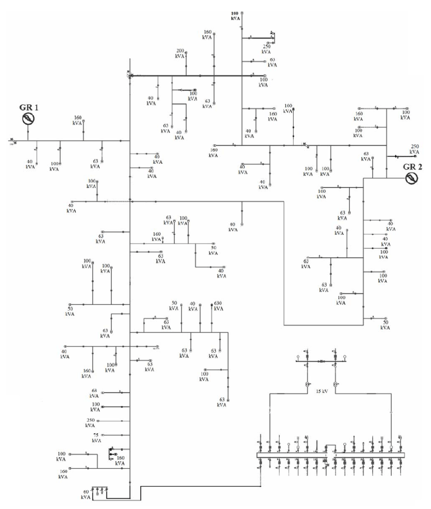
The MV line string fed from the second field of the transformer station of the analyzed grid was selected for the computational analysis, as shown in figure 1. Calculations for other MV lines fed from a given transformer station can be carried out in a similar way. The following criteria were analyzed in the proposed optimization model:
• minimization of grid failure rates (including SAIFI, SAIDI, average failure severity and failure durations), • optimization of power distributions, • minimization of voltage deviations at MV grid nodes, • minimizing technical losses in the distribution grid, • minimizing expenditures on upgrading the distribution grid under study,
For the optimization model used, limiting conditions relating to the maintenance of correct voltage levels and the maintenance of correct grid load conditions were taken into account. The values of the quantities determining the failure rate of cable lines were adopted on the basis of the studies described in papers [3, 5, 6].
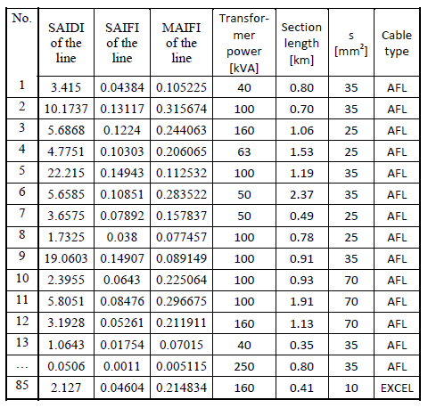
Table 1. Examples of selected actual section data at the ends of MV line branches (data excerpt)
.
In the first stage of the analyses, analyses using objective functions integrating the adopted optimization criteria were realized. In the second stage, calculations were also carried out to find sets of Pareto-optimal solutions. For this purpose, evolutionary algorithms adapted to multi-criteria calculations were used. The Matlab program and the “MatPower” package [24, 27] were used to perform the calculations. The purpose of the coding method adopted is to identify solutions for multivariate planning of grid upgrades, taking into account the use of distributed generation plant generation capacity.
The decision variables included in the optimization model determine the implementation (or lack thereof) of the upgrade of a specific element of the MV line under analysis. Encoding with a vector of real numbers was used.
In addition, the values of the decision variables also determine the choice of upgrade variant (if more than one variant is considered for a given device). The analyzed variants of section upgrades take into account the fulfillment of technical conditions regarding load capacity, throughput, voltage conditions, short circuit parameters.
The following optimized vector objective function was determined:
.
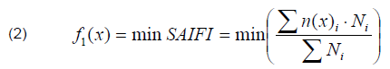
f1(x) – refers to the minimization of the SAIFI index (for the analyzed grid), which is a measure of the number of outages per customer (per year), and does not include outages shorter than 3 minutes:
.
whereas: ni – number of unscheduled outages at customers at a given location, Ni – number of customers at a given location,
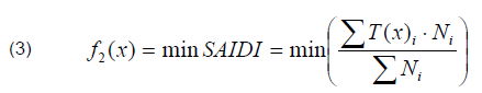
f2(x) – refers to minimization of the SAIDI index, determines the total duration of power outages in minutes that a customer in a given area of the distribution grid can expect (during the year):
.
whereas: Ti – annual outage time of customers at a given location, Ni – number of customers at a given location,
f3(x) – determines the minimization of power losses in the analyzed MV grid:
.
whereas: Rmi – resistance of the i-th section of the line after the upgrade,
f4(x) – the criterion function relates to the minimization of voltage deviations at the nodes of the analyzed field MV grid,
.
whereas: Ui– voltage at the i-th node, Uo – expected voltage, UN– rated voltage, n – number of nodes,
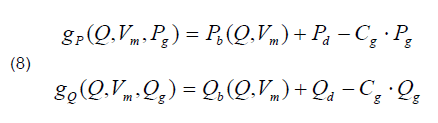
f5(x) – the criterion function for the criterion under consideration can be represented as the summation of cost functions for individual generation nodes:
.
where: Q – vector of values of voltage shift angles, Vm – vector of values of nodal voltages, Pg, Qg– vectors of values of generated active and reactive power,
In the developed computational model, the criterion of optimization of power distributions in the grid was taken into account (the description used in the Matpower package was used). Among other things, calculations of optimal power distributions can be carried out using the “runopf” function of the Matpower package, which performs calculations based on Lagrange’s theorem and Kuhn-Tucker conditions.
Fig.1. Diagram of the analyzed MV line of the field distribution grid.
These conditions are equivalent to the conditions for the existence of the saddle point of the Lagrange function, built on the function f(x) under the limitations gi(x).
The considered optimization task in its general form is described by the formulas [24, 27]:
.
The limiting conditions are a set of power balance equations described by formulas [24]:
.
where: Cg– connection matrix which can be defined so that its element (i, j) has a value of 1 if generator j is on bus i and 0 otherwise.
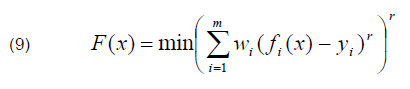
To write the aggregate form of the objective function, the distance function minimization methodology was adopted. The distance function method combines several criterion functions into a single aggregate based on a vector of (arbitrarily determined) ideal values. In this case, the optimal solution is the one that minimizes the distances between F(x) and the y vector.
.
whereas: r = 2 (most commonly used), the following set of weights was used for the optimization calculations for the criterion of reliability maximization and expenditure minimization: (w1=0.8, w2=0.2), (w1=0.7, w2=0.3) … (w1=0.2, w2=0.8). For subsequent calculations, the change of weight values for individual criteria is applied with a step of 0.1 or 0.05 (where the sum of all weights equals 1).
Various sets of criteria were analyzed in the completed computational analyses. In the results presented in the article (due to the volume of the article, selected results are included), instead of the criterion of optimizing power flow, the criterion of minimizing voltage deviations and the criterion of minimizing technical losses in the analyzed MV grid were taken into account.
The operators used in these algorithms changed the values of the decision variables within the limits set by the lower and upper bounds. The calculation methodology used makes it possible to determine the set of sections selected for modernization and the extent of modernization of individual MV lines. By decoding the solutions obtained, it is possible to identify options for upgrading individual sections of the grid. The crossover operator used is based on generating a vector of binary numbers and modifying (within assumed narrow limits) the transferred values of decision variables between solutions.
The calculations were carried out for the MV field electrical distribution grid shown in figure 1.
In the coding method adopted, the values of the decision variables were in the range of 0 ÷ 1. At the same time, the range was divided into four divisions, and depending on the value of the variable, the realization or lack of realization of modernization for the grid element associated with the decision variable was determined.
Based on the value of the decision variable, the option of upgrading a given section of the line was also determined (including the length of the route, the line reconstruction technology used).
Results of computational analyses
Computational analyses were carried out using Matlab and, in particular, the Matpower package [23, 26]. For this purpose, a description of the analyzed grid structure (node and branch data) was developed in the form of Matpower package files, which made it possible to carry out flow calculations.
It has been assumed that 30÷40% of the sections of the analyzed MV power line will be modernized, taking into account the modernization of both the end sections and in the so-called core of the line. A computer model of the MV field power lines adopted for analysis was developed. The analyzed section contains 150 nodes and about 250 branches (MV line sections). The description of the structure and parameters of the analyzed MV (15 kV) distribution grid was made according to the principles used in the Matpower package.
The description of the optimization model includes criterion objective functions, constraint conditions, coding procedures, recombination operators. In the completed analyses, grid loads were taken into account, and the generation capabilities of grid-connected distributed generation sources were considered (for local climatic conditions, the generation capabilities of local distributed generation sources were assumed).
In the main computational loop, the so-called “simulated evolution” calculations are carried out, within which the values of the criterion functions are calculated for the variants of modernization of the analyzed MV power line configured by the algorithm.
The evolutionary algorithm used for the computational analyses, implemented by Matlab’s ag function, used available recombination operators that create new solution variants. On the other hand, task-adapted procedures for encoding and decoding solutions were developed.
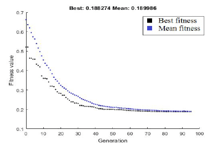
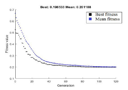
Initial analyses were realized for the formulated aggregate objective function described by equation (1). The results obtained are presented sequentially in figures 2÷3. These figures illustrate the course and effect of calculations to find solutions describing the range of projects for optimal MV line modernization plans with a new (compared to the optimization model from the works [21,22,23]) set of optimization criteria.
Fig.2. The course of calculations with the AG algorithm (the best solution obtained)
Fig.3. The course of calculations with the AG algorithm (the second best obtained solution)
The adopted coding method can be used to record alternative options for upgrading the MV line sections in the analyzed section of the field MV line. Modernization variants may differ in the different ways of routing the line, the technology used, as well as the diagnostic and switching equipment used, and the assumed length over which sections of the modernized MV line are rebuilt.
Figures 4, 5 show the execution of calculations with the assumption that two sources of distributed generation of 1 MW each are connected in the analyzed part of the grid. The calculations performed confirmed the feasibility of using the methodology described in the article to implement optimization calculations taking into account existing distributed sources or distributed sources planned to be installed in the grid.
Subsequent analyses, the outcomes of which are included later in the article, involved calculations considering two distributed sources in the form of photovoltaic farms of 1 MW each, as noted in figure 1.
In the realized analyses, reproducible results were obtained by obtaining solutions with the following consecutive values of the aggregating four criteria of the objective function: 0.198533, 0.198551, 0.198703, 0.198729, 0.198761, 0.198907, 0.199062.
Fig.4. The course of calculations with the AG algorithm (the best obtained solution for the variant with distributed generation)
Table 2 shows the best obtained values of the set of criterion functions selected for presentation for the solution found by the evolutionary algorithm that optimized the aggregate objective function. The aggregate functions were written using the method of minimizing the distance function between the values of the criterion functions and the values stored in the vector of ideal values. The found solution is illustrated in the diagram (fig. 11), where the MV line sections selected for upgrading are marked, which provides a graphic interpretation of the results.
Fig.5. The course of calculations with the AG algorithm (the second-best solution for the variant with distributed generation)
Tables 2 and 3 contain a description of the obtained solution in the form of a summary of the best obtained variants for upgrading the field MV line under study. The evolutionary algorithm used processes a population of 150 elemental vectors of real numbers, with a coded variant of the solution. Below are two decoded 150-element vectors in which each element of the vector is assigned a digit, which in turn determines the designated option for upgrading a given section of the MV line under analysis.
These two vectors differ very little (only at two positions) because they represent very similar variants of solutions. In these vectors, zeros indicate no upgrade while the numbers from 1 to 3 specify the upgrade variant for a given section of MV line.
Table 2. Values of criterion functions for the obtained solutions
.
Table 3. Values of reliability indexes of MV line sections after modernization
.
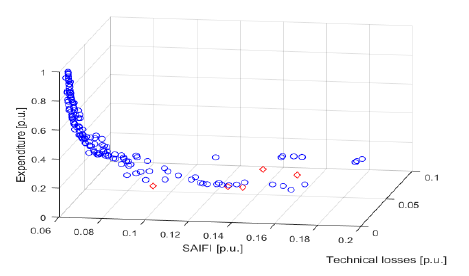
Calculations were also performed to graphically illustrate the obtained Pareto front for the selected two and three criteria for the analyzed problem. Figure 6 illustrates the results of calculations for the two criteria of financial input and reliability of the optimized MV line system. Single points (circles) for the aggregate approach are also plotted in this figure. These points were obtained in subsequent computational experiments in the implementation of which the weighting coefficients for the aggregate objective function for each criterion were empirically selected. This made it possible to find points distributed on the Pareto front for the problem under analysis.
Fig.6. Set of Pareto-optimal solutions with the NSGA II algorithm (Pareto front and single points)
In Figure 6, the SAIFI indexes calculated for the analyzed MV line (after normalization calculations) for the analyzed field MV line are used as a reliability criterion.
This indicator was calculated taking into account the structure of the supply routes of individual consumer nodes with the knowledge of the values of SAIFI indicators for individual sections of the analyzed fragment of the field MV grid. The calculation algorithms have been prepared so that calculations can also be made for all other reliability indexes such as p and q reliability indexes, SAIDI, MAIFI or average failure severity.
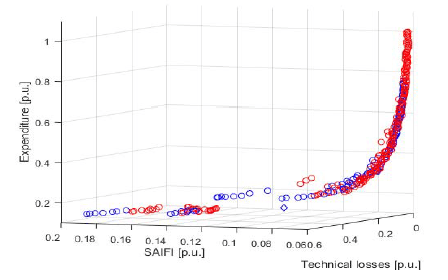
Computational analyses using algorithms (NSGA II, NSGA III [7, 8, 10]) that enable multi-criteria optimization calculations with independent treatment of individual criteria have also been realized [28, 29]. The non-dominated vectors of values calculated for the criterion functions form the Pareto front of the solutions. Figures 7 and 8 show the sets of Pareto-optimal solutions determined by each algorithm.
Computational analyses were carried out using normalizing conversions so that the individual values of the criterion functions fell within the range 0 ÷ 1, with arbitrary determination of the maximum and minimum values of the criterion functions in physical units.
The use of calculations normalizing the values of the criterion functions made it possible to unify the graphs presenting the results of the calculations and also allowed to present the concept and methodology of the calculations.
For the computational analyses, it was assumed that the maximum planned expenditures on grid modernization would allow to upgrade about 40% of the total length of the analyzed MV line string, taking into account the length of the line in the line core and all line branches. Fig. 7. Set of Pareto-optimal solutions for the three criteria (obtained with the NSGA II algorithm) Fig. 8. Set of Pareto-optimal solutions for the three criteria (obtained with the NSGA II algorithm with scores obtained for the aggregated approach)
In addition, in normalizing calculations (which facilitated the graphical presentation of the results of the calculations), such minimum and maximum values of financial outlays were selected so that, in particular, solutions close to the full assumed level of expenditures on the modernization of the analyzed MV line were analyzed.
Figure 9 shows the Parteo front obtained with the NSGA II algorithm for the analyzed problem, and indicates with rhombuses the obtained points using the aggregated objective function approach (these solutions are located in the middle part of the Pareto front) after introducing the weighting coefficients into the aggregated objective function, it is also possible to find points located in another part of the Parteo front.
Figures 9 and 10 illustrate the comparison of the sets of Pareto-optimal solutions determined for the analyzed task with the two algorithms (NSGA II and NSGA III [24, 29]). Each of the algorithms used has its own solution finding strategy [10]. The obtained results confirmed the convergence of the obtained solutions. The choice of the final solution in such a case is made by the decision-maker based on additional considerations.
The results for the aggregate objective function were obtained and a set of Pareto-optimal solutions was found for the analyzed problem. After realizing multivariate analyses with different algorithms, solutions were obtained that showed convergence of results.
For example, one of the best solutions obtained in the form of sets of projects that make up the optimal option for upgrading the MV line under study is illustrated in figure 11, the sections selected for upgrading are marked in red.
Fig.7. Set of Pareto-optimal solutions for the three criteria (obtained with the NSGA II algorithm)
Fig.8. Set of Pareto-optimal solutions for the three criteria (obtained with the NSGA II algorithm with scores obtained for the aggregated approach)
Fig.9. Pareto front obtained for the analyzed problem for two criteria with NSGA II (blue color) and NSGA III (red color) algorithms
Fig.10. Pareto front obtained for the analyzed problem for two criteria (second illustration of the results obtained with NSGA II (blue color) and NSGA III (red color) algorithms)
NSGA II and NSGA III algorithms were used to find the Pareto front for the problem under analysis. Among other things, the calculations used the algorithm available in Matlab’s gamultiobj function, which allowed to determine the Pareto front (for selected criteria), which is illustrated in figure 9.
Figure 11 shows in red those sections of the field MV power line that were selected for upgrading as a result of optimization calculations. This type of analysis can be carried out sequentially for all MV power lines coming out of the transformer station selected for analysis.
The solution variant shown in Figure 11 is characterized by the fact that sections of the line located primarily in the core of the line were selected for modernization projects, while sections from the line’s branches were selected to a lesser extent. This can be explained by the fact that the MV line analyzed was characterized by small cross sections, and the sections selected by the algorithm for modernization most urgently required modernization work.
Fig.11. Diagram of the analyzed MV line string with the elements selected for modernization, along with the description of the selected modernization variants
Summary
This article presents a modification and development of computational models previously presented in papers [21, 22, 23]. The computational optimization models from the aforementioned papers were adapted to finding optimal plans for modernizing large parts of the grid (fed from several transformer stations) with a limited number of criteria for an assumed time horizon of several years.
The modifications to the computational models proposed in this article make it possible to optimize reliability and efficiency for selected individual field MV power lines, while taking into account the local operating conditions of the MV lines and the power generated by GR distributed sources connected or planned to be connected.
For the calculations, heuristic methods were used in the form of evolutionary algorithms in the basic version (for the variant of calculations using the aggregate objective function) and the extended version for finding sets of Pareto-optimal solutions. The algorithms presented in the article provide opportunities to determine the scope of modernization activities in the analyzed MV lines fed from individual line fields of the transformer station. The results of the calculations are the optimal variants and scope of upgrading field MV power lines found by the algorithms.
REFERENCES
[1] Abedini M., Moradi M.H.: A combination of genetic algorithm and particle swarm optimization for optimal DG location and sizing in distribution systems. International Journal of Electrical Power & Energy Systems. Volume 34, Issue 1, January 2012, pp. 66–74. [2] Acharya N., Mahat P, Mithulananthan N.: An analytical approach for DG allocation in primary distribution network”, International Journal of Electrical Power & Energy Systems, vol. 28, 10, 2016, p.669-678. [3] Banasik K., Chojnacki A. Ł.: Effects of unreliability of electricity distribution systems for municipal customers in urban and rural areas, Przegląd Elektrotechniczny issue 05/2019, p. 179-183. [4] Bobric E. C., Cartina G., Grigoras G.: Fuzzy Technique used for Energy Loss Determination in Medium and Low Voltage Networks. Electronics and Electrical Engineering. – Kaunas: Technologija, 2009. – No. 2(90). – P. 95–98. [5] Chojnacki A.: Assessment of the Risk of Damage to 110 kV Overhead Lines Due to Wind. Energies, 2021, p. 1-14. [6] Chojnacki A.: Analiza niezawodności eksploatacyjnej elektroenergetycznych sieci Dystrybucyjnych, Monografie studia, rozprawy, Kielce, 2013. [7] Ciro G., Dugardin F., Yalaoui F., Kelly R.: A NSGA-II and NSGA-III comparison for solving an open shop scheduling problem with resource constraints. IFAC, International Federation of Automatic Control, 2016 s. 1272–1277. [8] Delbem A. C. B., Carvalho A. C. P. L. F., Bretas N. G.: Main chain representation for evolutionary algorithms applied to distribution system reconfiguration. IEEE Trans. Power Systems, vol. 20, no. 1, Feb. 2015, pp. 425-436. [9] Gawluk A.: Kierunki inwestowania a straty energii elektrycznej w sieci rozdzielczej. Przegląd Elektrotechniczny issue 3/2017. [10] Guohua Fang, Wei Guo, Xianfeng Huang, Xinyi Si, Fei Yang, Qian Luo, Ke Yan: A New Multi-objective Optimization Algorithm: MOAFSA and its Application. Przegląd Elektrotechniczny, R. 88 issue 9b/2012, p. 172-176. [11] Helt P., Parol M., Piotrowski P.: Metody sztucznej inteligencji – przykłady zastosowań w elektroenergetyce. Oficyna Wydawnicza Politechniki Warszawskiej, 2012. [12] Hong Y. Y., Ho S. Y.: Determination of network configuration considering multiobjective in distribution systems using genetic algorithms. IEEE Trans. Power Systems, 2005. – Vol. 20. – No.2– p. 1062–1069. [13] Kamrat W.: Metody oceny efektywności inwestowania w elektroenergetyce, Monografia Wydawnictwo PAN, Warsaw, 2004. [14] Kamrat W.: Selected information technology tools supporting for maintenance and operation management electrical grids, Bulletin of the Polish Academy of Sciences-Technical Sciences, 2021. [15] Kamrat W.: Selected problems of decision making modelling in power engineering, Sustainable Energy Technologies and Assessments, 2021 [16] Khushalani S., Solanki, J.M., Schulz, N.N.: Optimized Restoration of Unbalanced Distribution Systems. IEEE Transactions on Power Systems, no. 22, Issue 2. 2017, pp. 624-630. [17] Kumar Y., Das, B., Sharma, J.: Multiobjective, Multiconstraint Service Restoration of Electric Power Distribution System With Priority Customers. IEEE Transactions on Power Delivery, no. 23, Issue 1, 2008, p. 261-270. [18] Machowski J., Kacejko P., Robak S., Miller P., Wancerz M.: Badania systemów elektroenergetycznych w planowaniu rozwoju. Część 2. Analizy dynamiczne. “Wiadomości Elektrotechniczne,” vol. LXXXI, p. 3 -12, issue 8/2013, 2013. [19] Marzecki J., Drab M.: Obciążenia i rozpływy mocy w sieci terenowej średniego napięcia-wybrane problemy. Przegląd Elektrotechniczny, R.91, p. 192-195, February, Issue 2, 2015. [20] Marzecki J.: Modernization and development directions of low and medium voltage rural network, Przegląd Elektrotechniczny, 2019, vol. 95, s.67-70. [21] Nita W.: Optymalne planowanie przebudowy elektroenergetycznych terenowych sieci dystrybucyjnych SN za pomocą metod ewolucyjnych, Doctoral Dissertation, Kielce University of Technology, 2020. [22] Nita W., Filipiak S.: Planowanie przebudowy terenowych sieci dystrybucyjnych SN metodami ewolucyjnymi. Przegląd Elektrotechniczny, p. 92-98, Issue 4/2021. [23] Nita W., Filipiak S.: Optimization of the reliability of power electric distribution grids MV with the use of heuristic algorithms. Przegląd Elektrotechniczny, p. 50-56, R. 98, ISSUE 6/2022. [24] Ouyang, W.& Cheng, H.& Zhang, X.& Yao, L.& Bazargan, M.: Distribution network planning considering distributed generation by genetic algorithm combined with graph theory, Electric Power Components Systems, vol. 38, 3, 2019, p.325-339. [25] Parol M: Analiza wskaźników dotyczących przerw w dostarczaniu energii elektrycznej na poziomie sieci dystrybucyjnych. Przegląd Elektrotechniczny, p. 122-126, Issue 8/2014. [26] Parol M., Baczyński D., Brożek J.: Optimisation of Urban MV Multi-Loop Electric Power Distribution Networks Structure by Means of Artificial Intelligence Methods, Control and Cybernetics, 2012, vol. 41 (2012), p.667-689. [27] Pijarski P.: Optymalizacja heurystyczna w ocenie warunków pracy i planowaniu rozwoju systemu elektroenergetycznego. Monografia, Wydawnictwo Politechniki Lubelskiej, Lublin 2019 [28] Pijarski P, Kacejko P.: A new metaheuristic optimization method: the algorithm of the innovative gunner (AIG). Engineering Optimization.- 2019, vol. 51, nr 12, s. 2049-2068. [29] Pijarski P, Kacejko P., Miller P.: Advanced Optimisation and Forecasting Methods in Power Engineering—Introduction to the Special Issue. Energies 2023, vol. 16, nr 6, s. 1-20, [30] Sowiński J.: Forecasting of electricity demand in the region, January 2019E3S Web of Conferences, International Scientific Conference on Electric Power Engineering DOI:10.1051/e3sconf/20198401010. [31] Sowiński J.: Forecast of electricity supply using adaptive neuro-fuzzy inference system, May 2017, Conference: 2017 18th International Scientific Conference on Electric Power Engineering (EPE), DOI:10.1109/EPE.2017.7967248, [32] Sowiński J.: Use of load volatility description in modelling of energy balance in the section “electricity supply,” January 2017, Rynek Energii 128, p. 35-39.
Autorzy: dr inż. Wojciech Nita, PGE Dystrybucja S.A. Oddział Skarżysko-Kamienna, dr hab. inż. Sylwester Filipiak prof. PŚk, Politechnika Świętokrzyska w Kielcach, Katedra Elektrotechniki Przemysłowej i Automatyki, E-mail: filipiak@tu.kielce.pl
Source & Publisher Item Identifier: PRZEGLĄD ELEKTROTECHNICZNY, ISSN 0033-2097, R. 99 NR 11/2023. doi:10.15199/48.2023.11.05
Published by 1. Andrzej FARYŃSKI1, 2. Zbigniew ZIÓŁKOWSKI1, 3. Przemysław SUL2, Air Force Institute of Technology (AFIT) (1), Warsaw University of Technology (2) ORCID: 1. 000-0008-1232-2747; 2. 000-0002-7713-0271; 3. 0000-0002-4327-9334
Abstract. The article describes research, the main aim of which was to present the method of generating high-voltage impulses – solitons using a non-linear NLTL transmission line. Using such a line for the transformation of voltage pulses, the peak value of the voltage can be increased several times and the rise time and duration of the pulse can be significantly reduced. The results of laboratory tests presented in this article confirm the usefulness of this type of line for generating high-voltage nanosecond pulses.
Streszczenie. W artykule opisano badania, ktorych głownym celem było przedstawienie metody generowania wysokonapieciowych impulsówsolitonów za pomocą nieliniowej linii transmisyjnej NLTL. Stosując taką linię do transformacji impulsów napięciowych można kikukrotnie zwiększyć wartość szczytową napięcia oraz znacznie zredukować czas narastania I czas trwania impulsu.Wyniki badań laboratoryjnych przedstawionych w niniejszym artykule potwierdzają przydatność tego typu linii do generowania wysokonapieciowych nanosekundowych impulsów (Generacja solitonów wysokonapięciowych w nieliniowej linii transmisyjnej).
Keywords: Non-linear transmission lines (NLTL), pulse generation, electrical solitons. Słowa kluczowe: Nieliniowe linie transmisyjne (NLTL), generacja impulsów, solitony elektryczne.
Introduction
In recent decades, there has been much research work on the feasibility of using nonlinear transmission lines (NLTLs), for the generation of strings of high-voltage pulses, especially of high power, in the high RF as well as microwave frequency range [1 ], [2 ]. The pulses comprising such strings are known as solitons – a specific class of waves that propagate in non-linear dispersive media [3], [4], [5]. Each such soliton pulse propagates through the medium with little change in shape.
An NLTL is a long line filled with a material (medium) with non-linear dielectric and magnetic properties, with distributed constants: unit inductance L[H/m] and unit capacitance C[F/m]. The dielectric permeability of the medium depends on the electric field strength and or its magnetic permeability depends on the magnetic field strength. The construction of such a line is described in [2]. A section of such a line is shown in Figure 1.
Fig.1. NLTL line section with non-linear capacitance
Principle of the NLTL
The phase velocity of pulse propagation in a line with distributed constants is:
.
where: L – unit inductance [H/m], C – unit capacitance [F/m]
If the capacitance C decreases with increasing voltage, the further part of the pulse with a higher voltage value will travel faster than the initial part with a lower value, leading to the formation of an electromagnetic shock wave front with a very short rise time at the NLTL output. This is illustrated pictorially in Fig.2.
If a trapezoidal pulse is applied to the line input whose rising edge can be approximated by a series of small rectangular spikes of increasing amplitudes and decreasing widths, each narrow rectangular pulse generates a soliton in the NLTL that propagates along the line [7],[ 8], with solitons of larger amplitudes reaching the end of the line first. As a result, a radio frequency (RF) pulse generator based on the NLTL can transform the slowly varying input pulse into a stream of pulses of smaller width and higher peak power (sharpened) compared to the input pulse, each of which propagates along the line maintaining approximately its shape.
Fig.2. Schematic of soliton generation in a non-linear NLTL
Under experimental conditions it is much easier than a line with distributed constants to study a ladder line . Then L, C – are the inductance and capacitance of the elements of a single section of the ladder line. If the number of sections is n and the line has length d, the propagation velocity is:
.
where: d – length of line, n – number of line sections, L – section inductance, C – section capacitance
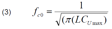
The shortest achievable rise time is limited by the Bragg cut-off frequency:
.
where: L – section inductance, CUmax – section capacitance for maximum voltage.
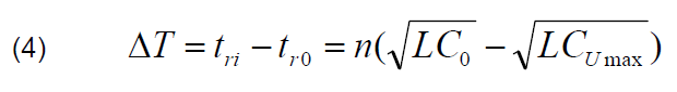
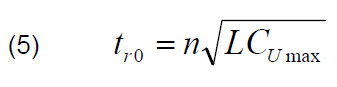
In what follows, this description will deal with the ladder line. The approximate value of the pulse rise time reduction caused by the LC ladder sections can be calculated by considering the time delay between the bottom of the amplitude and the peak of the propagating pulse as follows [9]:
.
where: tri is the rise time of the input signal, tro is the rise time of the output signal, n is the number of line sections, C0 is the initial capacitance (for voltage U0=0).
In the extreme case, the rise time of the output pulse is limited to a value corresponding to the Bragg cut-off frequency of the LC ladder.
.
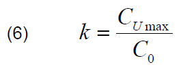
Assuming for simplicity that only the capacitance is nonlinear and that the non-linearity is characterised by a factor k:
.
Formula (2) can be transformed into the form (7) indicating that the assumed pulse sharpening can be achieved with capacitors with weaker non-linearity if a sufficient number of n sections are used.
.
In the paper [4], it was shown that in practice it is easier to produce a sufficient number of oscillations (i.e. a sequence of solitons) of reasonable amplitude when the NLTL is built from 50 or more sections.
Description of the construction of a non-linear transmission line
This article describes the construction of a non-linear ladder transmission line, in which commercially available (www.tme.pl) high-voltage 2.2nF/10 kV ceramic capacitors and inductances (chokes on ring ferrite cores of NiZn type with the symbol RTNIZN 10x6x3-U1000 of dimensions Ø10/Ø6/3, made of AN-100H material with initial permeability μr=1000) were used. Due to the lack of detailed data on the physical properties of the available 2.2nF/10 kV ceramic capacitors, their capacitance as a function of voltage was determined. The results of these measurements are shown in Fig.3.
Fig.3. Voltage characteristics of a 2.2nF/10 kV ceramic capacitor
The results presented show the strong voltage dependence of the capacitance of these capacitors.
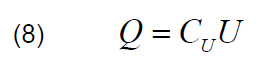
Determining additionally the electric charge accumulated in the capacitor (8), it can be seen that in the voltage range U > 2 kV the charge decreases with increasing voltage . Hence, the conclusion is that in this voltage range this capacitor will exhibit the characteristics of negative dynamic resistance
.
Using the ceramic capacitors discussed above, a ladder transmission line consisting of 10 LC sections was constructed according to the schematic diagram shown in Figure 4.
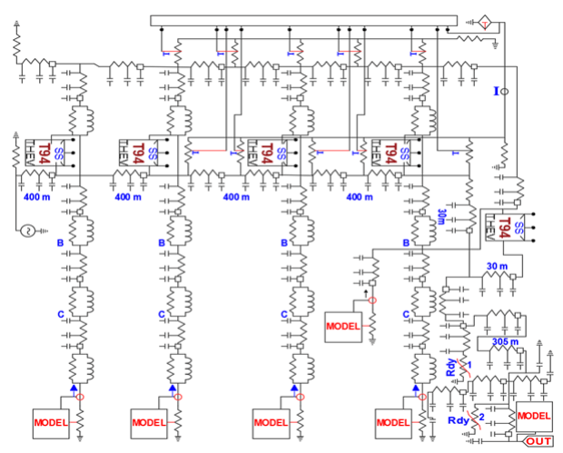
Fig.4. Schematic diagram of a non-linear transmission line (NLTL)
The high voltage pulse is applied to the line input when the TG1 controlled spark gap is triggered. The line input voltage was measured using divider R3/R4 with a division of 1000, the line output voltage was measured using divider R5/R6 with a division of 940. Measurements were carried out for capacitor C0 charging voltages between -3kV up to -6.5 kV. The view of the transmission line built and used in the study is shown in Figure 5.
Fig.5. View of the constructed non-linear transmission line (NLTL)
Description of the laboratory tests
In the first series of tests, measurements were carried out with a line consisting of a section with parameters L=1 μH and C=2.2 nF. The voltage at the input and output of the line was recorded on a RIGOL DS4024 digital oscilloscope with a frequency response of f = 500 MHz and a sampling frequency of 4 GHz.
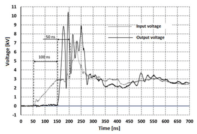
The pulse-solitons recorded at the line output (for a capacitor charging voltage C0 of UC0 = 3 kV) are shown in Fig. 6. There was a significant sharpening of the output pulse (from about 80 ns at the input to about 20 ns at the output) and about a 3.5-fold increase in amplitude (from 3 kV at the input to 10.5 kV at the output).
Fig.6. NLTL input and output signals for UC0= -3 kV
The propagation time of the pulse through the line was τ ≈ 100 ns, while the pulse reflected from the end of the line reached its input, where it was recorded, after a further 50 ns. By increasing the charging voltage to UC0 = -3.5 kV, pulses (solitons) with a maximum amplitude of 11.9 kV were recorded, as shown in Figure 7.
Fig.7. NLTL input and output signals for UC0= -3.5 kV
In the next series of tests, the choke inductance L was increased to 4 μH (doubling the number of turns) and the charging voltage of capacitor was increased to UC0 = -6 kV and UC0 = -6.5 kV.
The pulses (solitons) recorded at the line output for a charging voltage C0 of UC0 = -6 kV are shown in Figure 8, and for a charging voltage UC0 = -6.5 kV are shown in Figure 9.
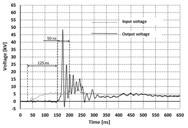
Fig.8. NLTL input and output signals for UC0= -6 kV
In these tests (for the case of a charging voltage value of UC0 = -6 kV), soliton pulses of surprisingly high amplitude were recorded at the output. The amplitude of the first pulse (leader) was Ul = 48 kV (i.e. an 8-fold multiplication of the amplitude was registered, from 6 kV at the input to 48 kV at the output) and with a 10-fold reduction in rise time (from 60 ns the input to 6 ns at the output). The propagation time of the wave the line was τ ≈ 125 ns, while the pulse reflected from the end of the line reached its input, where it was recorded, after a further 50 ns.
Fig.9. NLTL input and output signals for UC0= -6.5 kV
Fig.10. FFT spectrum of the output signal for a charging voltage of UC0 = -6.5 kV
Fig.11. Voltage characteristics of the failed 2.2nF/10 kV capacitor
For a charging voltage of UC0 = -6.5 kV, soliton pulses with a leader amplitude of Ul = 62 kV were recorded at the output, so there was a 9.5-fold amplitude multiplication (from 6.5 kV at the input to 62 kV at the output). The propagation time of the through the line was τ ≈ 105 ns, while the pulse reflected from the end of the line reached its input, where it was recorded, after a further 46 ns.
Obtaining soliton pulses with such high voltages may be due to the fact that there is an additional, synergistic effect of the non-linearity of the ferrite chokes used. By doubling the number of turns (a 4-fold increase in choke inductance) and doubling the charging voltage of the capacitance C0, saturation of the ferrite choke cores was caused (a multiple reduction in the magnetic permeability of the choke core material).
A spectral analysis (FFT) of the soliton package generated at a capacitor C0 charging voltage of UC0 = -6.5 kV is shown in Figure 10.
Unfortunately, after four attempts, the capacitors failed. Their capacitance decreased by about 2-3 times and the character of their capacitance dependence as a function of voltage changed, as shown in Figure 11. The probable cause of the capacitors’ failure was a change in the dielectric structure at such high voltages, but the capacitors showed no breakthrough when tested with a static voltage of 12 kV!
Conclusions
1. Applying a ladder line constructed from commercially available high-voltage 2.2 nF/10kV ceramic capacitors [11] and ferrite chokes, a sequence of solitons with amplitudes ranging from 10 kV to 60 kV and half-widths of a dozen to a few nanoseconds was generated.
2. The amplitude of the solitonic output pulses was multiplied up to 9 times to 62 kV (Fig. 8), with their halfwidth of 6 ns.
3. Spectral analysis of the generated soliton parcel with a maximum amplitude of 62 kV indicates that it was dominated by a frequency of approximately 74 MHz.
REFERENCES
[1] J.D.C.DARLING, P.W. SMITH , High-power pulsed RF extraction from nonlinear lumped element transmission lines, IEEE Trans.Plasma Sci., vol. 36, no. 5 pp. 2598-2603, Oct. 2008 [2] A.J. Fairbanks, T.D. Crawford, A.L. Garner – “Nonlinear transmission line implemented as a combined pulse forming line and high power microwave source”Rev. Sci. Instrum. 92, 104702 (2021) [3] P.W. Smith – „Pulsed, high power, RF generation from nonlinear dielectric lader networks – performance limits” Trans. of IEEE International Pulsed Power Conference 2011 [4] S. Ibuka, et. AI. – “Voltage amplification effect of nonlinear transmission lines for fast high voltage pulse generation “Trans, of IEEE International Pulsed Power Conference” 1997. [5] R.J. Baker, et all. – “Generation of kilovolt-subnanosecond pulses using nonlinear transmission line” Meas. Sci. Technol. 4, pp 893-895, (1993). [6] T. Kuusela, J. Hietarinta – “Nonlinear electrical transmission line as a burst generator” Rev. Sci. Instrum. 62 (9) pp 2266- 2270, September 1991 [7] M. Case et all – “Picosecond duration, large amplitude impulse generation using electrical soliton effects” Appl.Phys.Lett. Vol 60 (24), pp.3019-3021, June 1992 [8] L. P. Silva Neto, J.O.Rossi, J. J. Barroso, E. Schamiloglu – „High-power RF generation from nonlinear transmission lines with barium titanate ceramic capacitors“ IEEE Trans. Plasma Sci. 44, 3424 2016 [9] Anm Wasekul Azad – Development of puls power sources using self-sustaining nonlinear transmission lines and high-voltage solid state switches. – Dissertation in Electrical and Computer Engineering & Mathematics University of Missouri –Kansas City, 2012 [10]J. O.Rossi, P.N. Rizzo – „Study of hybrid nonlinear transmission lines for high power RF generation” IEEE Pulsed Power Conference 2009 [11] Karta katalogowa kondensatora 2,2 nF/ 10 kV – data sheet for capacitor 2,2 nF/ 10 kV – CC10K-2N2.pdf (tme.eu)
Authors: PhD, Eng Andrzej FARYŃSKI, Air Force Institute of Technology (AFIT), Księcia Bolesława 6 – street postal code: 01-494 Warsaw, post office box 96, Poland, E-mail:andrzej.farynski@itwl.pl PhD, Eng Zbigniew ZIÓŁKOWSKI, Air Force Institute of Technology (AFIT), Księcia Bolesława 6 – street, postal code: 01-494 Warsaw, post office box96, Poland, E-mail: zbigniew.ziolkowski@itwl.pl PhD, Eng Przemysław SUL, Warsaw University of Technology, Koszykowa Street 75, postal code: 00-662 Warsaw, Poland, E-mail: przemyslaw.sul@pw.edu.pl;
Source & Publisher Item Identifier: PRZEGLĄD ELEKTROTECHNICZNY, ISSN 0033-2097, R. 99 NR 11/2023. doi:10.15199/48.2023.11.06
Published by Jacek KOZYRA, Zbigniew ŁUKASIK, Aldona KUŚMIŃSKA-FIJAŁKOWSKA, Kazimierz Pulaski University of Technology and Humanities in Radom, Faculty of Transport, Electrical Engineering and Computer Science. ORCID: 1. 0000-0002-6660-6713, 2. 0000-0002-7403-8760, 3. 0000-0002-9466-1031
Abstract. Construction of new power lines is a complicated and long-lasting formal and legal process. The duration of the investments is extended by trade arrangements, public consultations in order to delimit line corridor, time required to obtain necessary decisions, permits, analyses and opinions necessary to implement an enterprise. The main goal of this publication is to conduct an analysis and present the variants of possibility of rebuilding of a power network in the aspect of increasing transmission potential of existing 110kV lines, taking technical and financial aspects into account.
Streszczenie. Budowa nowych linii elektroenergetycznych to skomplikowany i długotrwały proces formalno – prawny. Czas realizacji inwestycji wydłużają prowadzone uzgodnienia branżowe, prowadzone konsultacje społeczne w celu wytyczenia korytarza linii, oczekiwania na pozyskanie koniecznych decyzji, pozwoleń, analiz i opinii niezbędnych do realizacji przedsięwzięcia. Głównym celem publikacji jest przeprowadzenie analizy oraz przedstawienie wariantów możliwości przebudowy sieci elektroenergetycznej w aspekcie zwiększenia zdolności przesyłowych istniejącej linii 110kV z uwzględnieniem zagadnień technicznych oraz finansowych. (Zwiększenie zdolności przesyłowych linii 110 kV prądu przemiennego)
Keywords: High Temperature Wires, Wire capacity, Adaptive works, AFL, ACSR, ACSS/TW. Słowa kluczowe: Przewody wysokotemperaturowe, Obciążalność przewodu, Prace dostosowanie, AFL, ACSR, ACSS/TW.
Introduction
Construction of new lines is very expensive and problematic investment. New column structures, wires and additional equipment make costs of investment extremely high. Apart from financial aspect, there is also formal and legal battle connected with making land of the lines available and with obtaining relevant permits. These adversities make potential investors discouraged to build new modern power lines. Within last 15 years, there was a view of the so-called thermic modernization of existing lines. Thanks to application of the new generation of wires, HTLS (High Temperature Low Sag), significant change of structural solutions of old lines is unnecessary. This view is legitimate because in most of the lines built several dozen years ago, operating and static wires along with insulators and required equipment must be urgently replaced. New generation of HTLS allows not only to increase current parameters of load of the lines, but also improves resistance to wind and effects of icing of the wires.
Older lines of the National Power System were designed to capacity limit temperature of 40ºC [1-3]. Tests and analyses conducted by CIGRE (Conseil International des Grands Réseaux Électriques) showed that most of non-European and European power networks have different limit temperatures of the wires in the lines. For steel and aluminium wires in the United States temperature between 50 and 115 ºC are used, in Canada 75÷100ºC, in the Great Britain and Ireland 50÷75ºC, in the Scandinavian countries 50÷90ºC [3, 5]. The possibility of replacement of current steel and aluminium wires with high-temperature wires has become very attractive and apart from financial costs, there are no additional problems of legal and ownership character.
The goal of this publication is to conduct an analysis for the variants of rebuilding of power network illustrated with an example of existing 110 kV lines, taking technical and financial aspects into account. Four variants of adaptive works in the existing 110kV lines, which will allow to increase their transmission potential, were presented in this article. For each presented variant, time to do adaptive works and their cost were estimated.
Modernization of high-voltage overhead power lines
In the years 2017–2021, Polish Power Grids spent nearly PLN 6 billion for construction and modernization of transmission lines and stations. Within last 4 years, about 2700 km of tracks of 400 kV lines, 80 km of tracks of 220 kV lines and 6 new system substations were built. Until 2030, the following actions are planned [14]:
• 172 investments, • 3 597 km of new 400 kV lines, • modernization of 1 643 km of 400 kV lines, • calculated total value of expenditure is PLN 14 billion.
Performing duties of a transmission system operator, PSE are currently running more than 110 various investments. Above all, they include construction, expansion and modernization of high-voltage power lines and stations. Their goal is to ensure safe functioning of the National Power System and stable supply of electric energy to all consumers in a long-term perspective. Expansion and modernization of a transmission grid should be aimed at: creating safe working conditions of the National Power System, increasing security of supplying the areas of large urban agglomerations, increasing the role of transmission system in the National Power System, improving potential in the National Power System and voltage adjustment, power evacuation from connected sources, as well as expansion of interconnections [4, 6].
Among others, it requires substantial development of a structural transmission grid, structural changes of supply systems in crucial parts of Poland, allowing sources of energy of different production technology and various parameters to cooperate with each other, as well as photos of transmission functions with 110 kV distribution network, which takes place in many regions of Poland [7]. Among others, it requires substantial development of a structural transmission grid, structural changes of supply systems in crucial parts of Poland, allowing sources of energy of different production technology and various parameters to cooperate with each other, as well as photos of transmission functions with 110 kV distribution network, which takes place in many regions of Poland [10].
Modernization of overhead high-voltage power lines is mainly connected with increasing their thermal capacity and includes the following actions [8, 11, 16-18]:
• application of high-temperature low sag (HTLS), • construction of new or additional track of the lines, • application of the systems of monitoring and forecasting permissible current-carrying capacity of the lines, • modernization works.
Out of actions mentioned above, quick increasing of thermal-carrying capacity of overhead lines with no significant changes in structural solutions of old lines can be achieved by using high-temperature wires. The necessity to increase capacity results from the fact that large number of the overhead lines 110 kV in Poland was designed to work in design temperature of a wire of +40°C, which with ambient temperature +30°C and wind velocity 0,5 m/s guarantees to maintain permissible distances to the objects below the line [9].
In some studies, designed lines had design temperature of a wire of +60°C, and even +80°C. Assuming design temperature +80°C for AFL6-240 allows, under summer conditions, to load it with current of 645 A [12]. Such current, due to its invariability in time is called static current, whereas, maximum current determined based on actual weather conditions is commonly called dynamic current. Using dynamic capacity of the lines allows for better, more effective use of transmission potential of the lines. For example, for 6 m/s wind blowing perpendicularly to a line, capacity of the lines is increasing by 50% [13, 15].
Technical analysis of possibility of increasing current-carrying capacity of 110 kV lines
The comparison of ACSR and ACSS/TW phase conductors
For many years, phase conductors commonly applied in the National Power System have been AFL wires of ACSR type (Aluminium-conductor steel-reinforced). They are made of one or more concentric layers of a bearing steel wire and one or more conductive, reinforced layers of deformed aluminium wires. The requirements that such wires must meet made it necessary to develop diverse types of the wires in terms of diameters and relation of sections of steel to aluminium. For example, there are AFL-6 185mm2 , AFL-6 240mm2 and AFL-8 525mm2 . Due to constant growth of electric energy demand, phase conductors of this group are becoming insufficient. High mass of the wires and permissible operating temperature of +80°C translate into permissible current-carrying capacity of the lines. An alternative to this solution, more and more popular in the National Power System has become application of ACSS (Aluminium Conductor Steel Supported) high-temperature wires of low sag. They are wires of similar structure to ACSS/TW (Aluminium conductor steelSupported /Trapezoidal Wire) made of profile wires. Structure of a wire consists of a steel core in the braid of one or many layers of the wires, which allows increasing the degree of filling the section and increase current-carrying capacity while maintaining diameter of a wire similar to the one from ACSR family. ACSS/TW can work in a constant way, without damages in high temperature of +200°C with no loss of mechanical properties. Annealed aluminium applied in the wires makes it more elastic and most of the loads rest on steel core, which has supporting function of ACSS. An equivalent of AFL-6 240mm2 ACSR is ACSS/TW Hawk 242-AL0/39-MEHST. Diameter of ACSS/TW is lower than ACSR with a similar section. Structure and materials that ACSS is made of allow to reach lower mass of a wire in comparison with traditional ones. Resistance of ACSS/TW Hawk 242-AL0/39-MEHST is much lower than resistance of AFL-6 240mm2 ACSR. It means that their application in modernized and newly built lines will result in lower losses and reduction of CO2 emission connected with losses. Parameter that we should pay attention to is modulus of elasticity (Young modulus), which for ACSR is more than 2,5 times higher than for ACSR [19]. Young modulus is a very significant parameter in construction of the wires that determines elasticity of the wires and sags of the wires in the spans of the lines. Table 1 shows the comparison of technical parameters of the examples of ACSR and ACSS/TW Hawk.
Table 1. The comparison of technical parameters of AFL-6 240 and ACSS/TW Hawk
.
Most of 110kV power lines in the National Power System, operating temperature of phase conductors max. +40°, +60° or +80°C. ACSS, due to its special structure and parameters, allows to increase permissible operating temperature of the lines up to even +200°C, making it possible increasing flow of current in a line while maintaining similar sags of the wires in the spans in comparison with ACSR working in maximum temperature of +80°C.
In order to determine current-carrying capacity of ACSR AFL-6 240mm2 and ACSS/TW HAWK 242-AL0/39-MEHST, assumed ambient temperature in summer conditions was +30°C and in winter: +20°C. Sun exposure of the wires in summer: 1000 W/m2 , in winter: 770 W/m2 . Emission factor and absorption coefficient of a wire – 0,5. Wind velocity – 0,5 m/s perpendicularly to a wire. Table 2 shows relation between the value of sag of the wires and temperature of the wires.
Fig.2. Chart of capacity of the wires – summer period
Fig.2. Chart of capacity of the wires – winter period
Charts of capacity of ACSR AFL-6 240mm2 and ACSS/TW HAWK, relations were presented on figure 1 and 2.
Increasing maximum current-carrying capacity gives the possibility of modernization of existing 110 kV lines, that is, replacement of existing ACSR with ACSS without the necessity of replacement of columns and foundations with new ones. For 300 meter span and weather conditions assumed while determining current-carrying capacity, the values of sag of the wires to temperature of a wire were determined in Table 3.
Table 3. The value of sag for ACSR AFL-6 240mm2 and ACSS/TW HAWK 242-AL0/39-MEHST
.
.
Fig.3. Chart of relation between the value of sag of a phase conductor and temperature
The value of a sag of the wires depending on temperature of ACSR AFL-6 240mm2 and ACSS/TW HAWK, the relations are presented on figure 3.
The values of the sags of ACSS/TW HAWK 242- AL0/39-MEHST phase conductors in maximum operating temperature of +200°C are comparable with the sags of ACSR AFL-6 240mm2 phase conductors in permissible temperature of +80°C. It is important because in replacement of phase conductors with ACSS in the existing lines will not reduce existing, normative distances between phase conductors and the ground and remaining alternately used objects.
Replacement of ACSRs with ACSS/TW high-temperature wires
An analysis of replacement of the wires includes assessment of possibility of increasing current-carrying capacity of high-voltage lines illustrated with an example of existing 110 kV overhead line, which is 12,67 km long. The scope of analysis includes preparing and modelling of existing state of 110 kV lines in a specialist software for designing overhead lines, PLS-CADD (Power Line Systems – Computer Aided Design and Draft). Input data to software along with geodesic measurements of existing state of the lines were entered in order to prepare a model of lines. Using this software, existing state of the lines was reconstructed and existing stress in the phase conductors and static wires was determined. Then, the scope of adaptive works to do depending on assumed value of current-carrying capacity of the lines was determined. While preparing a list of necessary adaptive works, the possibility of doing the following works was checked in the first place:
• shortening suspension strings in order to increase distance from alternately used objects inside the span, • possibility of adjustment of sags of existing wires, • making columns higher through assembly of catalogue insert making the bottom part of a column higher.
The possibility of replacement of single columns and replacement of existing ACSR AFL-6 240mm2 with ACSS high-temperature wires was considered. Final effect of the analysis shows adaptive works that are necessary to reach required current-carrying capacity of 110 kV lines depending on accepted variant. Financial aspects were considered while preparing such variants. Time estimated to do specific adaptive works, device required to do such works and cost estimate for each variant were prepared.
Existing 110 kV line was designed and built so as not to exceed maximum operating temperature of phase conductors, that is, +40°C. In such temperature, phase conductors can be loaded with current not exceeding:
• in the summer period, for ambient temperature (To= +30°C), wind velocity (V = 0,5m/s), sun exposure (Ps=1000W/m2) ─ 131A, • in the winter period (To = +20°C, V=0,5m/s, Ps=770W/m2): ─ 364A.
Increasing transmission potential is possible through adjustment of the phase conductors to operating temperature of +80°C or replacement of existing wires with a new, high-temperature ACSS. However, it requires modernization of the lines. Therefore, there were the following assumptions – 4 variants of modernization depending on accepted current-carrying capacity. For each variant, all required adaptive works will be presented that need to be done due to required normative distances to the ground and alternately used objects.
Variant 1
Adaption of existing AFL-6 240 mm2 ACSRs to work in maximum temperature +80°C. Target current-carrying capacity of the wires: summer – 609A, winter – 686A.
Variant 2
Replacement of existing ACSR AFL-6-240 mm2 phase conductors with new ACSS/TW Hawk 242-AL0/39-MEHST high-temperature wires, adapted to operating temperature of +80°C. Target current-carrying capacity of the wires: summer – 622A, winter – 700A.
Variant 3
Replacement of existing ACSR AFL-6-240 mm2 phase conductors with new ACSS/TW Hawk 242-AL0/39-MEHST high-temperature wires, adapted to operating temperature of +120°C. Target current-carrying capacity of the wires: summer – 833A, winter – 886A.
.
Fig.4. Determining current-carrying capacity of ACSS/TW Hawk 242-AL0/39-MEHST in PLS-CADD
Fig.5. Panel of PLS-CADD to enter weather data and capacity of the lines in order to determine temperature of the wires
Variant 4
Replacement of existing ACSR AFL-6-240mm2 phase conductors with new ACSS/TW Hawk 242-AL0/39-MEHST high-temperature wires, adapted to maximum operating temperature of +160°C. Target current-carrying capacity of the wires: summer – 983A, winter – 1023A. An example of determining current-carrying capacity of ACSS/TW Hawk 242-AL0/39-MEHST was presented on fig. 4.
Based on:
• Geodesic measurement (location of the columns, span length, how high are wires hanged, size of sags), • Conditions during measurements (measured air temperature, wind velocity and direction, specific level of sun exposure), • Momentary value of load current of the lines, accepted emission factor and absorption coefficient.
Temperature of the wires at the moment of taking geodesic measurements was determined. Temperature of the wires was generated in PLS-CADD after entering data mentioned above. Figure 5 shows a panel of entering data of PLS-CADD.
Actual stress in the wires was determined based on a spatial model and calculated temperature of the wires that measurement of this model was made. Based on that, in PLS-CADD, existing stress in the wires was determined. In accordance with PN-E-05100-1:1998 „Overhead power lines. Design and construction. Alternating current lines with bare operating wires”, the highest permissible stress in steel and aluminium phase conductors or aluminium-alloy ones may not exceed 40 % resistance to normal stretching. While determining maximum stress in the wires in a given pull-off section, we must consider:
• permissible strength of applied wire, in which maximum tension in the wires may not exceed in no point 40% of RTS (rated power tearing off a wire), • conditions that column was designed for, which are specified in the specification sheets of columns.
While determining permissible stresses in AFL6 240mm2 phase conductors, three examples were analysed:
Example 1 – Maximum stress/tension in the wires due to strength of structure of the of columns
In the analysed 110 kV line, S24 lattice columns were applied, which in accordance with specification sheet, columns were adapted to hanging on AFL-6 240mm2 phase conductors with a stress of 100MPa in -5Sn condition (temperature -5° with additional load with normal hoar frost). In accordance with specification sheet, AFL-6 240mm2 has a diameter of 21,7mm and total section s = 276,2mm2 , rated power tearing RTS off = 84600 N. Stress in AFL6 240mm2 (s =276,2mm2) is 100MPa, which gives the value of tension:
100MPa ꞏ 276,2mm2 = 276200N (in -5Sn condition).
Therefore, different wire of similar parameters can also be hanged, but with an assumption that in -5Sn condition, the value of tension of a new wire does not exceed the value of tension of 276200N like for AFL-6 240mm2 in -5Sn condition.
Example 2 – Maximum stress for AFL-6 240mm2 due to strength of a wire
In accordance with PN-E-05100-1:1998, permissible tension in the phase conductors of pull-off section may not exceed 40% RTS of a wire, that is:
84600 Nꞏ0,4 = 33840 N,
which gives power of tension of the wires
F = 33840 ÷ 276,2 =122,5 MPa
That is, „normal” stress for AFL-6 240mm2 due to stretching is 122,5 MPa. Therefore, permissible stress due to strength of a column: 100 MPa and permissible stress due to strength of a wire: 122,5 MPa. That is, as a value of „normal” stress in AFL-6 240mm2 we accept lower value from the ones above, that is, 100 MPa.
Example 3 – „Reduced” stress for AFL-6 240mm2
In accordance with PN-E-05100-1:1998, permissible „reduced” tension in the phase conductors of pull-off section may not exceed 28% RTS of a wire, that is:
84600 Nꞏ0,28= 23688 N,
which gives power of tension of the wires
F = 23688 ÷ 276,2=85,7 MPa
That is, the value of „reduced” stress in AFL-6 240 mm2 is assumed as 85,7 MPa. To sum up, we assume the following stresses for AFL-6 240 mm2 :
Determining permissible stresses in ACSS/TW Hawk 242- AL0/39-MEHST phase conductors, example no. 4 was analysed.
Example 4 – „Reduced” stress for ACSS/TW Hawk 242- AL0/39-MEHST
ACSS/TW Hawk 242-AL0/39-MEHST, in accordance with specification sheet, has a diameter of 20,03mm and total section s = 281,3 mm2 , rated power tearing RTS off = 84400 N. While designing a new wire, we should assume that stress of ACSS in -5Sn condition -does not exceed tension of 276200N, like for AFL-6 240mm2 . It means that the value of normal stress is:
F = 276200 ÷÷ 281,34 = 98,2 MPa
In accordance with PN-E-05100-1:1998, permissible „reduced” tension in the phase conductors of pull-off section may not exceed 28% of RTS of a wire, that is: 84400ꞏ0,28 = 23632N, which gives
F =23632÷281,34 = 84 MPa
The value of „reduced” stress in ACSS/TW Hawk 242- AL0/39-MEHST is assumed as 84 MPa. To sum up, we assumed the following stresses for ACSS/TW Hawk 242- AL0/39-MEHST:
Existing 110 kV line with 45 spans was modelled in PLS-CADD and permissible operating temperature of phase conductors and permissible current-carrying capacity of the lines were determined. Table 4 shows the values of maximum temperature that phase conductors can work in the existing state, that is, without doing any adaptive works. Red color was used to distinguish the spans, in which phase conductors do not reach required operating temperature of +40°C before adaptive works, because there are no required normative distances from the ground and alternately used objects.
Table 4. A list of spans allowing the work of phase conductors of the lines in temp. +80°C
.
.
Based on the results obtained in Table 4, it was found that 110 kV line in the existing state can’t work in temperature that it was designed for, that is, +40°C. In the spans no. 2 – 3, 22 – 23, 28 – 29, 29 – 30, 35 – 36, 41 – 42 and 42 – 43, there are no required normative distances from alternately used objects. In the spans no. 22 – 23 and 29 – 30, maximum operating temperature of phase conductors is 0°C, which means that line should be disconnected because it is dangerous for safety of people. Adaptive works must be immediately done. In the existing state, to maintain normative distances between phase conductors and the ground and alternately used objects, phase conductors can work in temperature of 0°C. As it results from calculations for design temperature of a wire, that is, 0°C, capacity of the lines is 0 [A]. It results from obvious fact that wire heats up to such temperature only from solar energy. In order to determine operating temperature of phase conductors for specific current-carrying capacity, the following operating weather conditions of the lines are assumed:
• in the summer period, for ambient temperature (To= +30°C), wind velocity (V = 0,5m/s) of perpendicular direction to a wire, sun exposure (Ps=1000W/m2 ), emission factor and absorption coefficient of a wire, each by 0,5,
• in the winter period, for ambient temperature (To=+20°C), wind velocity (V= 0,5m/s) of perpendicular direction to a wire, sun exposure (Ps=770W/m2 ), emission factor and absorption coefficient of a wire, each by 0,5,
Table 5 shows the comparison of maximum value of current-carrying capacity of lines depending on type of a wire and maximum operating temperature of conductors.
Table 5. Comparison of the maximum current carrying capacity of the line
.
For current-carrying capacity of the wires presented in Table 5 , simulation was made in PLS-CADD determining the works that must be done in 110 kV line for phase conductors to work in specific temperature. To meet the requirements of 4 variants of capacity, a list of required adaptive works and their cost were presented in Table 6.
Table 6. A list of adaptive works for variant 1, 2, 3 and 4
.
Conclusions
ACSSs have, due to its structure, to a large extent flat sag depending on temperature and after exceeding the so-called knee point, growth of temperature causes very low growth of sag, which allows to fully use its potential in high temperatures. Special structure of a wire makes it possible to reach much higher capacity of the lines in comparison with AFL-240mm2 ACSRs. Moreover, as it was shown in the comparison of AFL-6 240mm2 with ACSS/TW Hawk 242- AL0/39-MEHST, ACSS high-temperature wires generate the lowest losses working in increased temperature, with the same load like in ACSR wires. The main parameter is much lower resistance of ACSS. Therefore, it can be said that reduction of transmission losses will make investment cost-effective after a few years.
Conducted technical analysis based on existing WN 110 kV power line showed that by the application of ACSS hightemperature wires allowed to significantly increase its transmission potential without interference to structural solutions of existing lines. Replacement of phase conductors from typical ACSR AFL-6 240 mm2 with ACSS made it necessary to do required adaptive works such as: reinforcing and raising existing supporting constructions and in one case, the necessity to replace a column. After completion of the works mentioned above, 110 kV line will be able to work in temperature of even +160°C. It will allow to reach the following current-carrying capacity of the wires: summer – 983 A, winter – 1023 A, where in the existing state, line could work only in temp. +40°C and maximum load: summer – 131 A, winter – 364 A.
Increasing transmission potential through modernization of existing objects is much more attractive solution in financial terms than construction of new lines. As it was shown in the analysis, reasonable solution is replacement of commonly applied ACSRs with ACSS high-temperature wires because they are one of the cheapest high-temperature wires available on the market.
A significant aspect of all modernization works is cost connected with adaptation of 110 kV lines to type of the operating wires. There is a cost estimate for each of four variants, which differs significantly depending on a variant of scope of adaptive works. Final result of a cost estimate was presented in the article and it was found that modernization of 110 kV lines with ACSS/TW Hawk 242- AL0/39-MEHST adapted to operating temperature of +80°C is cheaper by more than 12% than adaptation of existing AFL-6 240mm2 ACSRs to work in maximum temperature of +80°C. Another proposed variants with ACSS/TW Hawk 242-AL0/39-MEHST adapted to operating temperature of +120°C and +160°C, are solutions that are by 30% and 64% more expensive in comparison with the best financial variant, however their target current-carrying capacity of the wires is much higher. When this parameter will be a determinant, proposed solutions can be applied because an alternative is construction of a new line, which is much more expensive.
REFERENCES
[1] Ntuli M., Mbuli N., Motsoeneng L., Xezile R. Pretorius J. H. C., Increasing the capacity of transmission lines via current uprating: An updated review of benefits, considerations and developments, 2016 Australasian Universities Power Engineering Conference (AUPEC), Brisbane, QLD, Australia, (2016), 1-6, https://doi.org/10.1109/AUPEC.2016.7749338 [2] Popczyk J., (red.): Bezpieczeństwo elektroenergetyczne w społeczeństwie postprzemysłowym na przykładzie Polski. Monografia, (2009), Wydawnictwo Politechniki Śląskiej, Gliwice [3] Kubek P., Metody analizy przewodów elektroenergetycznych pod względem cieplnym i mechanicznym, Elektryka, 2-3 (2014), 21-39, Wydawnictwo Politechniki Śląskiej, Gliwice [4] Kocot H., Kubek P., Analiza poprzecznego rozkładu temperatury w przewodach elektroenergetycznych, Przegląd Elektrotechniczny, 93, 1093 (2017), 132-135, https://doi.org/10.15199/48.2017.10.31 [5] Mbuli N., Pretorius J. H.C., Potential Factors for Multi-Criteria Evaluation of Capacity Uprate in Relation to New Transmission Line Projects, 2022 IEEE PES/IAS PowerAfrica, Kigali, Rwanda, (2022), 1-5, doi: 10.1109/PowerAfrica53997.2022.9905294. [6] Plan rozwoju w zakresie zaspokojenia obecnego i przyszłego zapotrzebowania na energię elektryczną na lata 2023–2032, Polskie Sieci Elektroenergetyczne Operator S.A., Warszawa Dokument główny, XI 2022 [7] Dołęga W., Planowanie rozwoju sieciowej infrastruktury elektroenergetycznej w aspekcie bezpieczeństwa dostaw energii i bezpieczeństwa ekologicznego. Monografia, (2013), Oficyna Wydawnicza Politechniki Wrocławskiej, Wrocław [8] Riba J.R, Bogarra S., Gómez-Pau Á., Moreno-Eguilaz M., Uprating of transmission lines by means of HTLS conductors for a sustainable growth: Challenges, opportunities, and research needs, Renewable and Sustainable Energy Reviews, 134 (2020), 110334, ISSN 1364-0321, https://doi.org/10.1016/j.rser.2020.110334 [9] Ntuli M., Mbuli N., Motsoeneng L., Xezile R. Pretorius J.H. C., Increasing the capacity of transmission lines via current uprating: An updated review of benefits, considerations and developments, 2016 Australasian Universities Power Engineering Conference (AUPEC), Brisbane, QLD, Australia, (2016), 1-6, https://doi.org/10.1109/AUPEC.2016.7749338 [10] Dołęga W., Rozwój sieci przesyłowej w aspekcie bezpieczeństwa dostaw energii. Przegląd NaukowoMetodyczny „Edukacja dla bezpieczeństwa”, 3 (2014) [11] Dołęga W., Modernizacja sieciowej infrastruktury elektroenergetycznej w aspekcie planowania jej rozwoju, Rynek Energii, 1 (2015), 12-19 [12] Babś A., Samotyjak T., Monitorowanie i prognozowanie dopuszczalnego obciążenia linii napowietrznych 110 kV, Elektro Info, 7-8 (2011), 70-74 [13] The thermal behavior of overhead conductors. Technical Brochures CIGRE, 207, (2002) [14] https://www.pse.pl/inwestycje/informacje [15] Meyberg R.A., De Barros M.T.C. Lima A.C.S., New Approach for Ampacity Calculation of Overhead Lines With Steel-Cored Conductors, IEEE Transactions on Power Delivery, 38 (2023), No 2, 1011-1019, https://doi.org/10.1109/TPWRD.2022.3203668. [16] Nuchprayoon S., Chaichana A., Performance Comparison of Using ACSR and HTLS Conductors for Current Uprating of 230-kV Overhead Transmission Lines, 2018 IEEE International Conference on Environment and Electrical Engineering and 2018 IEEE Industrial and Commercial Power Systems Europe (EEEIC / I&CPS Europe), Palermo, Italy, 2018, 1-5, https://doi.org/10.1109/EEEIC.2018.8493888 [17] Reddy S., Mitra G., Investigations on High Temperature Low Sag (HTLS) Conductors, IEEE Transactions on Power Delivery, 35 (2020), No. 4, 1716-1724, https://doi.org/10.1109/TPWRD.2019.2950992 [18] Silva A.A.P., Bezerra J.M.B., Applicability and limitations of ampacity models for HTLS conductors, Electric Power Systems Research, 93 (2012), 61-66, ISSN 0378-7796, https://doi.org/10.1016/j.epsr.2012.07.003 [19] Prasetyo H., Sudiarto B., Setiabudy R., Analysis of Knee Point Temperature (KPT) determination on High Capacity Low Sag (HCLS) conductors for optimizing the ampacity load and sag on the overhead transmission lines system, IOP Conference Series: Materials Science and Engineering, 1098 (2021), Computer Science https://doi.org/10.1088/1757-899X/1098/4/042021
Authors: dr hab. inż. Jacek Kozyra, prof. UTH Rad., Uniwersytet Technologiczno-Humanistyczny im. Kazimierza Pułaskiego w Radomiu, Wydział Transportu, Elektrotechniki i Informatyki, ul. Malczewskiego 29, 26-600 Radom, E-mail: j.kozyra@uthrad.pl.; prof. dr hab. inż. Zbigniew Łukasik, UTH Rad., Wydział Transportu, Elektrotechniki i Informatyki, ul. Malczewskiego 29, 26-600 Radom, E-mail: z.lukasik@uthrad.pl; dr hab. inż. Aldona KuśmińskaFijałkowska, prof. UTH Rad., Wydział Transportu, Elektrotechniki i Informatyki, ul. Malczewskiego 29, 26-600 Radom, E-mail: a.kusmińska@uthrad.pl;
Source & Publisher Item Identifier: PRZEGLĄD ELEKTROTECHNICZNY, ISSN 0033-2097, R. 99 NR 11/2023. doi:10.15199/48.2023.11.08
Published by 1. Ali N. HAMOODI1, 2. Safwan A. HAMOODI2, 3. Farah I. HAMEEDI3, Northern Technical University (1), Northern Technical University (2), Northern Technical University (3), Iraq ORCID: 1. 0000-0003-0991-3538; 2. 0000-0001-9346-5680; 3. 0000-0003-1742-6959
Abstract. Photovoltaic systems are impacted by the quantity and temperature of sunshine. Due to the competing nature of solar radiation, PV systems operate inefficiently. A variety of maximum power point tracker (MPPT) approaches are utilized to increase the solar system’s influence. Incremental optimization (IO), one of the more established MPPT algorithms, provides great steady-state productivity and tracking accuracy over a broad range of shifting atmospheric conditions. Characterizing solar PV features at various irradiances using Matlab or Simulink. The simulation’s findings seemed to agree with the different planned PV module efficiencies. In conclusion, it has been found that this optimization technique enhances the PV system’s tracking efficiency and response time, leading to dependable grid operation.
Streszczenie. Na systemy fotowoltaiczne ma wpływ ilość i temperatura nasłonecznienia. Ze względu na konkurencyjny charakter promieniowania słonecznego systemy fotowoltaiczne działają nieefektywnie. W celu zwiększenia wpływu Układu Słonecznego stosuje się różne podejścia do śledzenia punktu maksymalnej mocy (MPPT). Optymalizacja przyrostowa (IO), jeden z bardziej uznanych algorytmów MPPT, zapewnia doskonałą produktywność w stanie ustalonym i dokładność śledzenia w szerokim zakresie zmieniających się warunków atmosferycznych. Charakteryzowanie właściwości fotowoltaiki słonecznej przy różnym natężeniu promieniowania przy użyciu Matlaba lub Simulinka. Wyniki symulacji wydawały się zgadzać z różnymi planowanymi wydajnościami modułów fotowoltaicznych. Podsumowując, stwierdzono, że ta technika optymalizacji poprawia wydajność śledzenia systemu fotowoltaicznego i czas reakcji, prowadząc do niezawodnego działania sieci. (Udoskonalanie elektrowni fotowoltaicznej w oparciu o algorytm optymalizacji przyrostowej)
The semiconductor materials used in PV panels are utilized to produce electrical energy when they are exposed to sunlight. The amount of electrical energy produced depends on the semiconductor material’s energy gap, which must not exceed a certain level. Solar intensity, temperature, and resistance all affect a PV cell’s output efficiency. In order to find the PV operating point that agrees with the demodulation of maximum power from the array, a control method known as maximum power point tracking (MPPT) is required [3], [4].
The purpose of the current work is to model a boost converter utilizing a conventional equation modeling technique rather than a circuit model. The buck/boost converter model was created using a leading equation-based model that enables the input voltage of the converter and the output voltage of a specific PV module to be changed by varying the duty cycle, allowing for the tracking of the maximum power point as environmental conditions change [5–7].
The known incremental conductance approach is fully examined and compared to a predefined system in this work. The model is realized using a DC/DC boost converter supplying a load and an MPPT controller. The results of the simulation indicated that the MPPT algorithm used in the solar PV system is suitable. In order to run efficiently, a power plant’s BOS (balance of system) must meet the preconditions for plant development. Grid inverters, mounting hardware, cables, and connectors are all supplied by default in the BOS. The lifespan record comprises the energy used by the operational authority, and regular system maintenance is required for the solar PV plant to produce power properly [3], [9].
Solar PV cells have a limited conversion efficiency, and their output power is fully dependent on irradiance and temperature under non-uniform operating conditions (NUOCs). As a result, reliable tracking of global power peaks to achieve maximum power point tracking is a critical problem for optimal SPV array usage in grid-connected or isolated modes of operation [10], [11].
The excrescence power that generated is forward to the utility grid and the consumer acquires compensated for it. Similarly, the consumer has been drawn the electricity from the grid and pacy for the units which used. Fig.1 represents the on-grid solar PV system [12], [3].
Fig.1. On-grid solar PV system.
Literature review
K. Ramesh and et al., (2018) studied on incremental conductance algorithm, they applied this algorithm on maximum power point tracking (MPPT) controller. It has been concluded that the incremental conductance algorithm for studied system didn’t able to eliminate the study state oscillation and the output power reduces by 8-59% from the maximum power [1].
Praveen Kumar and et al., (2021) studied on 100kW PV system connected with grid (on-grid). They incremental conductance algorithm for MPPT controller. Matlab/Simulink were used to model the proposed system. The revised MPPT algorithm was shown to be capable of boosting the dynamic and steady-state functioning of the PV system, as well as tracking the maximum amount of solar light and efficiently supplying maximum power for the PV array [2].
System and components
The gird connected PV system installed in one governorate of India country described briefly in this section. The whole components of 100kW grid connected PV system illustrated in Fig 2 [13].
Fig.2. Matlab modeling of 100kW grid connected PV system.
PV array
The PV array is considered as the main component of the PV system, which is comprised of 400 half-cut polycrystalline PV modules connected in series and parallel. Every 25 PV modules are connected in series to form 4 PV strings connected in parallel. The total output parameters of the PV array at STC are 100kW [12].
Fig.3. Flowchart of Incremental Conductance based MPPT.
Maximum power point tracking
PV energy production is highly dependent on the number of factors, like sun irradiation and ambient temperature. PV modules contain unique maximum power points that are related to current solar irradiation and current weather temperature values, in addition to voltage and current relationships that are not linear. MPPT algorithms are used to get the current and maximum power from PV modules by controlling DC-DC converters and successfully regulating the obtained power and voltage values from PV modules under different situations. There are a lot of MPPT algorithms to choose from, however this paper focus on incremental conductance. Fig.3, illustrates the procedure of Incremental Conductance based MPPT. Incremental Conductance Technique as a MPPT algorithm [14-15]. The boost converter parameters are listed in table 1.
Table 1. Boost converter parameters
.
Three-phase hybrid inverter
Three-level IGBT switches three-phase voltage source inverter (VSI) is used to convert DC-link voltage to AC voltage. The inverter switches are derived using pulse width modulation (PWM) technique. According to IEEE standard the frequency of several kilowatt grid connected inverter should be not greater than 6kHz [8], the switching frequency of inverter is 5kHz. The output of inverter connected to grid at the point common coupling (PCC) through L filter. For this reason, the inverter most be fully synchronized with utility grid [17].
Operation scenario
The operation scenario is done by exam the PV system performance under STC 1000W/m2 solar irradiance and 25oC temperature. After transient period the solar irradiance to 250W/m2 and the generated power from PV array 100kW. After that the solar irradiance increased gradually to reaches maximum value. Fig.4 shows the Simulink results obtained from grid connected PV system under different situations [18].
Fig.4. PV system performance under different situations
Fig.5. PV system under different situations.
From the above Figure the maximum output power has been obtained at solar irradiance 1000W/m2 and the low output power (14kW) has been obtained at solar irradiance 250W/m2. The variation of duty cycle between 0.45 – 0.5. Fig.5 represents the variation of V.PV and I.PV as time variance with respect to Idiod-PV value. The low power was obtained at mid time scale (1.5sec).
From Fig.5 the maximum power was (1000kW) was stable at time equal to (2.7sec.) and the minimum power was (25kW) at time equal to (15sec.).
Conclusions
In this paper, the behaviour of the 100kW grid-connected PV system was simulated and experimentally analysed under different operation conditions. The proposed system provided high-quality power to the local load and the utility grid. The real-time parameters such as averaged generated power, maximum generated power. The obtained results show that the grid-connected PV system was the best solution to meet the power generation shortage and reduce the stress on the transmission lines and low voltage transformers especially under peak load.
Acknowledgment – We would like to give our special thanks to our affiliation of Northern Technical University (NTU)-Technical College of Engineering, Mosul-Iraq.
Authors: Ali N. Hamoodi, ali_n_hamoodi74@ntu.edu.iq. Safwan A. Hamoodi, safwan79azb@ntu.edu.iq., Farah I. Hameedi, farah.isam@ntu.edu.iq. Northern Technical University, Technical College of Engineering /Mosul.
Source & Publisher Item Identifier: PRZEGLĄD ELEKTROTECHNICZNY, ISSN 0033-2097, R. 99 NR 10/2023. doi:10.15199/48.2023.10.35
Published by 1. Afaneen Anwer Abbood1, 2. Hanan Mikhael D. Habbi2, University of Technology-Iraq, Baghdad, (1) , University of Baghdad, Dept. Of Electrical Engineering, Baghdad, Iraq (2) ORCID: 1. 0000-0003-3995-8307; 2. 0000-0003-4982-4345
Abstract. Renewable energy can make the utility grid unstable by causing some problems, such as frequency fluctuations, voltage surges, and power instability because of the inconsistency of renewable energy resources. This paper focused on studying the effect of intermittent renewable energy represented by a PV-integrated grid on the frequency system response and grid voltage surge. Heuristic Optimization methods, Teaching learning-based optimization (TLBO), and particle swarm optimization (PSO) have been utilized to optimize the penetration of PV energy enhancing the supply frequency response. Both optimization methods have been implemented with different values of irradiance. Although they have similar performances, the simulation result showed that the TLBO method has a slightly better low-frequency oscillation than the PSO method. It is found that the TLBO algorithm presents a good power quality response of the grid-connected system. This is due to the fact of TLBO is faster than the PSO algorithm because it does not need specific parameters. The system is applied to a feeder in a distribution network in Baghdad power sector. The results are obtained by using the MATLAB package.
Streszczenie. Energia odnawialna może spowodować niestabilność sieci elektroenergetycznej, powodując pewne problemy, takie jak wahania częstotliwości, skoki napięcia i niestabilność mocy z powodu niespójności zasobów energii odnawialnej. W artykule skupiono się na badaniu wpływu przerywanej energii odnawialnej reprezentowanej przez zintegrowaną sieć fotowoltaiczną na odpowiedź systemu częstotliwości i udary napięcia sieciowego. Aby zoptymalizować przenikanie energii fotowoltaicznej, zwiększając charakterystykę częstotliwościową zasilania, zastosowano metody optymalizacji heurystycznej, optymalizacji opartej na uczeniu się (TLBO) i optymalizacji roju cząstek (PSO). Obie metody optymalizacji zostały zaimplementowane przy różnych wartościach natężenia napromieniowania. Chociaż mają one podobne właściwości, wynik symulacji pokazał, że metoda TLBO charakteryzuje się nieco lepszymi oscylacjami w zakresie niskich częstotliwości niż metoda PSO. Stwierdzono, że algorytm TLBO zapewnia dobrą odpowiedź dotyczącą jakości energii w systemie podłączonym do sieci. Wynika to z faktu, że TLBO jest szybszy od algorytmu PSO, ponieważ nie wymaga określonych parametrów. System stosowany jest w polu zasilającym w sieci dystrybucyjnej w sektorze energetycznym Bagdadu. Wyniki uzyskuje się za pomocą pakietu MATLAB. (Optymalizacja heurystyczna penetracji energii fotowoltaicznej w celu zapewnienia odporności na wahania częstotliwości systemu)
Index Terms: Power system distribution, Frequency fluctuations, Teaching Learning Based Optimization (TLBO), PSO Słowa kluczowe: Dystrybucja systemu elektroenergetycznego, wahania częstotliwości, optymalizacja oparta na nauczaniu (TLBO), PSO
Introduction
Despite the ease of use of renewable energy due to the impulses of nature regularly renewable energy has many prospective advantages over fossil power generation [1-3], the rapid or intermittent penetrations of renewable energy resources such as wind energy and solar PV energy cause serious problems to the power system fluctuations in the voltage and system frequency [4-6]]. These problems require accurate and satisfactory solutions to ensure that the integrated grid works efficiently. On the other hand, the penetration of wind energy (renewable energy resource) may lead to a percentage change in the frequency performance of the power system [7, 8]. Many researchers discussed these problems. Ref [9] proposed a tuned virtual filter that connected to a wind energy integrated grid to mitigate the system frequency fluctuations. It has been shown that the proposed system does not affect the efficiency of wind energy. Ref [10] studied and compared the number of strategies to control the drop frequency and the step response for a high PV system penetration without curtailing solar PV energy, it explored the storage energy for initial frequency response and implemented the strategies on the Texas grid, USA. Rajiv K and M Akbari,[11] suggested a PV-STATCOM to enhance the frequency and power system stability deviation by combining two controllers’ rapid frequency control and power oscillation damping to control the real power. Whereas Ref [12] designed and implemented the combination of the two controllers for simply real power control of Type 4 wind turbines. Mao Yang, et.al. [13] proposed a tabular model to study and analyze the effects of constraints of the renewable energy grid model in terms of output power, voltage, and frequency fluctuations.
On the other hand, some researchers minimized the frequency deviation using different intelligent techniques such as [14-19] a fuzzy-based frequency control incorporating the active frequency response constraints into the optimal development model, while [20] proposed the Mixed Integer Linear Programming (MILP) method. Refs. [21-23] developed a real-time nonlinear curve fitting maximum power point tracking. This paper proposed an integrated grid system for a distribution feeder to migrate to a distributed generation model for higher availability of electricity from a variety of sources (solar, and DG power). The effect of the intermittent load on the system frequency percentage changes for the PV-integrated grid was studied. The algorithms were applied to a feeder in the Baghdad power sector in a distribution network. The system includes 15kW, fixed PV solar panels, combined with a DC- AC inverter of 25kW, and the 15-kW annual hourly peak demand, with peak day energy use of 3.85kWh. The total PV generation is 96.68kW (4.03kW average).
Simulation Model
The proposed method depends on the amount of total power generated from each energy resource that is connected to the feeder. The optimal generated power from each source annually might cover the required demand load, considering the weather variations. The whole proposed system is shown in Fig.1. The frequency and grid voltage responses under different values of irradiance were compared based on two optimization methods (TLBO and PSO).
Also, the statistical distribution over time was analysed according to the availability of resource data (DG size and solar PV energy penetration at a specific period). The simulation layers include energy resources, data information, and optimization algorithms as shown in Fig.2.
Fig.1. The complete system with MATLAB/Simulink
Fig.2. Simulation layers
The PV system efficiency is given in Equation (1)
.
The annual capacity factor is given in Equation (2)
.
The annual capacity factor can be (0.25- 0.3) depending on the weather.
Heuristics Optimization
Heuristics optimization uses combinational computations, which depend on the practical experience of the system that will be studied. There are some specific cases that will be discussed in detail in the results section. The goal is to make the difference between the capacity produced from the energy sources attached to the system close to the requirements of the load and the utilization of capacity produced from solar cells in peak load processing. In the case of cloudy weather conditions or in the event of sunset (night-time), as the solar cells do not produce energy, therefore, the system will depend on the national grid.
Teaching Learning-Based Optimization (TLBO)
The influence of the teacher has affected the output of the learners. This algorithm does not require the specific parameters as in PSO algorithm. Therefore, it could obtain the optimum values with less computation time and operations [1], [2]. There are two modes for TLBO: the teacher phase and the learner phase. Let gets start to explain these modes:
1) Teacher Phase
To understand the modelling of this algorithm, it might illustrate the following factors: min F(x) limits
.
N=No. of iterations; P=size of population; Fval=determined by TLBO ; BFval=the best fitness function value in each iteration; Po= the population at the end of the specified no.of iteration.; For gen=1 to N;
Partner selection for all students begin of the teacher factor generation of a new solution bounding of the solution evaluation of the solution Greedy selection
2) Leader phase
Generation of a new solution Bounding of the solution evaluation of the objective function greedy selection
Power balance of the microgrid
.
In this paper, it takes 5 learners and 2 subjects. That means the decision variables are 2. According to our decision variables, the objective function or test function becomes:
.
After that, it can calculate the values of Pgrid and PDG taking the values of N=50, and P=10. According to the size of the iteration N=50, and it will start the evaluation before the start of the iteration. Since, the TLBO has two parameters which are the size of the population (P) and the size of the iteration (N). Therefore, the convergency of the TLBO does not change or vary. That’s results to minimize the oscillation in the power mismatch equality between the generation and the demand will be slightly slow.
Particle Swarm Optimization (PSO)
An evolutionary computation algorithm PSO gives the optimal solution of the energy penetration from a variety of energy resources [3]. It needs an initialization of the system parameters, no of the particles = 100 and the maximum iteration time is 0.2sec as well as the parameters of the power demand and weather conditions. Then, each particle will generate the initial speed I from 1 to 100 to obtain the global and best values. After that, each particle is updated with its speed to get the optimal value. Obtaining the optimal value of the grid and demand power for the energy management of a microgrid using PSO takes a time to reach the optimal value, that will show an oscillation in the quality of the result. In other word, PSO has a low convergence for the frequency response in energy management microgrid system. In contrast, the implementation of the PSO will be simple than the TLBO method [4]. Nevertheless, PSO has an ability to get a local convergence that will results to be a slow computation and will effect on the response quality.
Results And Discussion
The complete system shown in Fig 1 is implemented with MATLAB/Simulink with a constant irradiance (1000W/m2). Fig. 3 shows the frequency response and the frequency deviation for the PSO algorithm. It can be illustrated from the results that; the frequency response has an oscillation down to 48Hz and it takes about 10sec to reach a steady state value at 50Hz. This oscillation is because of the penetration of the power from the solar PV into the microgrid. Fig. 4 shows the grid voltage in volt and per unit. The irradiance and temperature values are kept constant taking as 1000W/m2 and 25Co respectively. The parameters for Baghdad feeder are shown in Table 1. It is cleared from Fig. 4 that the grid voltage (Vg) will be stable within a short time based on TLBO. Meanwhile, the PSO takes a time to solve the oscillation problem.
It can be observed from Fig.4 (a) and (b) when the irradiance is kept constant that the frequency deviations for TLBO and PSO frequency response can be detected and eliminated within 5 sec. The simulation results for the grid voltage results using PSO as shown in Fig. 5(a) take about 5sec to reach its rated value while the grid voltage as shown in Fig.5 (b) using TLBO algorithms have a fast response and reaches the grid voltage (400V) abruptly without an oscillation.
Fig.3. Frequency response using (a) PSO , (b) TLBO
Fig. 4. Grid voltage using PSO (a) PSO, (b) TBLO
Table 1. The Parameters of the Baghdad feeder
.
Variable Irradiance
In this section, the effect of changing the irradiance on the frequency response and the voltage grid have been studied using two optimization algorithms (PSO and TLBO). The irradiance applied to PV solar (1000W/m2 at zero sec to 500W/m2 at 1.5 sec) as shown in Fig.5.
When the PV solar irradiance is suddenly changed from 1000W/m2 to 500 W/m2 at 1.5sec as shown in Fig. 6, the frequency response for PSO and TLBO methods as shown in Fig. 6. The frequency response from TLBO has a good and an optimal control. However, it is obvious that the change in frequency response is rapidly slow down with TLBO algorithm. While the frequency response of the microgrid system from the PSO results takes a long time to settle down to 50Hz. In addition, the amplitude of the frequency oscillations is high for the PSO results compared with that of TLBO algorithms. That is the frequency response for TLBO frequency response can be detected and eliminated within less than 0.25 sec, while that of the PSO results will be more than 5 sec to settle down. Not only the system response of the TLBO algorithm is faster than that of the PSO results but also the overshooting in the frequency response has better results using TLBO. The results show satisfactory observations of the fluctuations elimination and oscillation amplitude within a considerable time.
The simulation results when the irradiance is changed as shown in Fig. 7, the grid voltage results using PSO as shown in Fig.7 (a) take about 5sec to reach its rated value while the grid voltage as shown in Fig.7 (b) using TLBO algorithm have a fast response and reaches the grid voltage (400V) abruptly without an oscillation.
The comparison of frequency response using PSO and TLBO optimization methods under sudden changes in PV solar irradiance reveals that TLBO demonstrates superior performance with faster and more stable responses, effectively eliminating fluctuations and minimizing overshooting. In contrast, PSO exhibits slower settling time and higher amplitude of oscillations, making it less efficient in achieving grid stability. TLBO’s ability to quickly regulate frequency and its reduced computational burden make it a promising and practical choice for real-world applications in microgrid systems, with the potential for further refinement to enhance its performance.
Fig.5. Irradiance (W/m2)
Fig.6. Frequency response using (a) PSO, (b) TLBO
Fig.7. Grid Voltage using (a) PSO, (b) TLBO
It can be concluded that the sudden decrease in irradiance results in the rapid decrease of active power output from PV solar systems. Consequently, the power deviation (difference between load power and generated power) returns to zero. However, under the PSO method, it is obvious that the amplitude of frequency response oscillation and grid voltage surges is higher using PSO algorithm compared to that of TLBO algorithm. Since it can reach the optimal value with a significant value of time computation with less oscillation or disturbances on the obtained responses.
Conclusion
This paper considers two optimization methods PSO and TLBO to optimize the penetration of the power to the microgrid system through the PV energy resources. This penetration of power influences the grid frequency and grid voltage surges. However, it is a challenge to perform MPPT with a variable irradiance. The paper compares the frequency and voltage oscillation of the microgrid using two optimization methods (PSO and TLBO) under different irradiance values. PSO algorithm has a low convergence for the frequency response in energy management microgrid system. The implementation of the PSO is simple than the TLBO method. Nevertheless, PSO has an ability to get a local convergence that led to a slow computation and that will influence the response quality. On the other hand, the TLBO has two parameters which are the size of the population (P) and the size of the iteration (N), the size of the iteration is proposed to be N=50, and it is starting the evaluation before the starting of the iteration. Therefore, the convergence of the TLBO does not change or vary. That’s results to minimize the oscillation in the power mismatch equality between the generation and the demand. It can be concluded that the TLBO algorithm gives an optimal value of the power that can be obtained from the solar PV energy resource. It can significantly observe the reduction of the frequency oscillation and can further improves the power quality with MPPT based on TLBO with a significant value of time computation with less oscillation or disturbances on the frequency and voltage responses. It is found that the TLBO algorithm presents a good quality convergence to the frequency and better voltage response of the grid connected system.
REFERENCES
[1] H. L. W. a. W. G.Scott, “Distributed Power Generation, planning and evaluation”, (2000), Publisher: New York : Marcel Dekker.,” 2000. [2] R. Takahashi, Umemura, A., Tamura, J., Kimura, M., & Hino, N, “Simulation analyses of stabilization control of power system frequency fluctuations resulting from wind farm output by gas turbine thermal power plant. https://doi.org/10.1002/eej.23321,” Electrical Engineering in Japan, vol. 214, no. 2, 2021. [3] J. Hossain, & Mahmud, A, ” Renewable Energy Integration. https://doi.org/10.1007/978-981-4585-27-9,” Springer Singapore., 2014. [4] B. Al Kindhi, Lasminto, U., Triana, M. I., Damarnegara, S., & Anavatti, S. G. , “4. Sensor and internet of things based integrated inundation mitigation for smart city. International Journal of Electrical and Computer Engineering (IJECE), 13(3), 2695. https://doi.org/10.11591/ijece.v13i3.pp2695-2703,” 2023. [5] Ahmed Abbas Abdul-Hamza and Hanan M. Habbi, “[6] (2016). Fault detection and diagnosis based on artificial neural network. International Journal of Scientific & Engineering Research, VOL. 7, NO. 5, 2016, PP- 1690-1697. https://www.ijser.org/research-paper-publishing-may2016_page8.aspx.,” 2016. [6] T. S. Tagare, & Narendra, R, “Lifetime enhanced energy efficient wireless sensor networks using renewable energy. https://doi.org/10.11591/ijece.v13i3.pp3088-3098,” International Journal of Electrical and Computer Engineering (IJECE),, vol.13, no. 3, p. 3088, 2023. [7] M. G. Dozein, Chaspierre, G., Mancarella, P., Panciatici, P., & van Cutsem, T. , ” Frequency Response From Solar PV: A Dynamic Equivalence Closed-Loop System Identification Approach,https://doi.org/10.1109/JSYST.2021.3051938,” IEEE Systems Journal,, vol. 16, no. 1, pp. 713–722, 2022, doi: https://doi.org/10.1109/JSYST.2021.3051938. [8] L. Zhou, Chen, Y., Luo, A., Guerrero, J. M., Zhou, X., Chen, Z., & Wu, W., “Robust two degrees-of-freedom single-current control strategy for LCL-type grid-connected DG system under grid-frequency fluctuation and grid-impedance variation. https://doi.org/10.1049/iet-pel.2016.0120,” IET Power Electronics,, vol. 9, no. 14, pp. 2682–2691, 2016. [9] I. Isknan, Asbayou, A., Hamid Adaliou, A., Ihlal, A., & Bouhouch, L., “Comparative study and simulation of advanced MPPT control algorithms for a photovoltaic system. https://doi.org/10.11591/ijeecs.v30.i1.pp46-56.,” Indonesian Journal of Electrical Engineering and Computer Science,, vol. 30, no. 1, p. 46, 2023. [10] A. M. Abdul Hussain, & Habbi, H. M. D. , “11. Maximum Power Point Tracking Photovoltaic Fed Pumping System Based on PI Controller. 2018 Third Scientific Conference of Electrical Engineering (SCEE), 78–83. https://doi.org/10.1109/SCEE.2018.8684120,” 2018. [11] R. K. Varma, & Akbari, M. , “Simultaneous Fast Frequency Control and Power Oscillation Damping by Utilizing PV Solar System as PV-STATCOM. https://doi.org/10.1109/TSTE.2019.2892943,” IEEE Transactions on Sustainable Energy, vol. 11, no. 1, pp. 415–425, 2020. [12] D. Rimorov, Joos, G., & Kamwa, I. , “Design and implementation of combined frequency/oscillation damping controller for type 4 wind turbines., https://doi.org/10.1109/PSCC.2016.7540909,” 2016 Power Systems Computation Conference (PSCC), pp. 1–7., 2016. [13] M. Yang, Cui, Y., & Wang, J., “Multi-Objective optimal scheduling of island microgrids considering the uncertainty of renewable energy output. https://doi.org/10.1016/j.ijepes.2022.108619,” International Journal of Electrical Power & Energy Systems, vol. 144, 2023. [14] M. M. A. Awan, Javed, M. Y., Asghar, A. B., & Ejsmont, K., ” Performance Optimization of a Ten Check MPPT Algorithm for an Off-Grid Solar Photovoltaic System,https://doi.org/10.3390/en15062104,” Energies, vol. 15, no. 6, p. 2104, 2022, doi: https://doi.org/10.3390/en15062104. [15] P. P. Kulkarni*, & Deshmukh, S. P. , “Different Converter Topologies for Solar Photovoltaic System with methods for Maximum Power Point Tracking Algorithms. , . https://doi.org/10.35940/ijitee.J1202.0981119,” International Journal of Innovative Technology and Exploring Engineering, vol. 8, no. 11, pp. 1112–1118, 2019. [16] J. E. Mendoza, López, M. E., Fingerhuth, S. C., Peña, H. E., & Salinas, C. A., “15. Low voltage distribution planning considering micro distributed generation..https://doi.org/10.1016/j.epsr.2013.05.020,” Electric Power Systems Research,, vol. 103, pp. 233–240, 2013. [17] A. Q. Al-Shetwi, Issa, W. K., Aqeil, R. F., Ustun, T. S., Al-Masri, H. M. K., Alzaareer, K., Abdolrasol, M. G. M., & Abdullah, M. A. , ” Active Power Control to Mitigate Frequency Deviations in Large-Scale Grid-Connected PV System Using Grid-Forming Single-Stage Inverters https://doi.org/10.3390/en15062035,” Energies, vol. 15, no. 6, p. 2035, 2022, doi: https://doi.org/10.3390/en15062035. [18] K. Liao, Xu, Y., Yin, M., & Chen, Z., ” A Virtual Filter Approach for Wind Energy Conversion Systems for Mitigating Power System Frequency Fluctuations . https://doi.org/10.1109/TSTE.2019.2922302,” IEEE Transactions on Sustainable Energy, vol. 11, no. 3, pp. 1268–1277, 2020. [19] R. Rajan, Fernandez, F. M., & Yang, Y., ” Primary frequency control techniques for large-scale PV-integrated power systems: A review.https://doi.org/10.1016/j.rser.2021.110998,” Renewable and Sustainable Energy Reviews,, vol. 144, 2021. [20] Q. Zhang, Xie, J., Pan, X., Zhang, L., & Fu, D. , “A Short-Term Optimal Scheduling Model for Wind-Solar-Hydro-Thermal Complementary Generation System Considering Dynamic Frequency Response. https://doi.org/10.1109/ACCESS.2021.3119924,” IEEE Access, vol. 9, pp. 142768–142781., 2021. [21] M. M. Mohamed, el Zoghby, H. M., Sharaf, S. M., & Mosa, M. A., “Optimal virtual synchronous generator control of battery/supercapacitor hybrid energy storage system for frequency response enhancement of photovoltaic/diesel microgrid.https://doi.org/10.1016/j.est.2022.104317,” Journal of Energy Storage, , vol. 51, 2022. [22] V. D. Paduani, Yu, H., Xu, B., & Lu, N., “A Unified PowerSetpoint Tracking Algorithm for Utility-Scale PV Systems With Power Reserves and Fast Frequency Response Capabilities, https://doi.org/10.1109/TSTE.2021.3117688,” IEEE Transactions on Sustainable Energy, vol. 13, no. 1, pp. 479–490., 2022. [23] K. Saadaoui, Rhazi, K. S., Mejdoub, Y., & Aboudou, A. , “Modelling and simulation for energy management of a hybrid microgrid with droop controller, https://doi.org/10.11591/ijece.v13i3.pp2440-2448,” International Journal of Electrical and Computer Engineering (IJECE), , vol.13, no. 3, p. 2440, 2023.
Source & Publisher Item Identifier: PRZEGLĄD ELEKTROTECHNICZNY, ISSN 0033-2097, R. 99 NR 12/2023. doi:10.15199/48.2023.12.07
Published by 1. Bahri PREBREZA, 2. Nuri BERISHA1*, 3. Bashkim STATOVCI, Faculty of Electrical and Computer Engineering, University of Prishtina ORCID: 1. 0000-0003-1950-026X; 2. 0000-0001-8615-637X; 3. 0000-0002-6840-0778
Abstract. Power systems might experience electrical problems or power outages, due to atmospheric discharges. The quality of the protection from atmospheric overvoltages will increase the life of the equipment and the reliability of the electrical system. The model for switching overvoltage calculations on the 400 kV transmission line of Kosovo Power System is analysed with ATP/EMTP software. Controlled and uncontrolled switching and controlled and uncontrolled repetitive switching of the 400 kV transmission line are analysed.
Streszczenie. W systemach zasilania mogą wystąpić problemy elektryczne lub przerwy w dostawie prądu z powodu wyładowań atmosferycznych. Jakość ochrony przed przepięciami atmosferycznymi zwiększy żywotność sprzętu i niezawodność instalacji elektrycznej. Model do obliczeń przepięć łączeniowych na linii przesyłowej 400 kV Systemu Elektroenergetycznego Kosowa jest analizowany za pomocą oprogramowania ATP/EMTP. Analizie poddano przełączanie sterowane i niekontrolowane oraz sterowane i niekontrolowane powtarzalne przełączanie linii przesyłowej 400 kV. (Analiza przepięć łączeniowych i zabezpieczeń przed przepięciami atmosferycznymi dla rozdzielni 400kV w Systemie Elektroenergetycznym Kosowa z wykorzystaniem ATP/EMTP)
Keywords: Power outages, atmospheric overvoltages, surge arresters, ATP/EMTP. Słowa kluczowe: Przerwy w dostawie prądu, przepięcia atmosferyczne, ograniczniki przepięć, ATP/EMTP.
Introduction
Electricity is becoming more and more important for everyday life, and the demand for the electricity from households and economic growth is increasing day by day. Most modern facilities require stable electricity supply generated by power plants, facilities such as schools, hospitals, the entertainment sector, various businesses, government properties, etc. Therefore, it is important that electricity is provided in a stable manner, which is made possible by effective control systems in the transmission system. However, the complex transmission network that carries power over a wide area can experience electrical faults or power outages, due to atmospheric discharges striking on the transmission network. This often causes blackouts in the power system [1,2].
Overvoltages are divided into internal overvoltages, external (atmospheric) overvoltages and induced overvoltages. Internal overvoltages appear because of the state of the electrical system. So, the source of these overvoltages is the power system itself. External overvoltages appear in the electrical system because of the atmospheric discharges. Induced overvoltages appear in the system in case of voltage flash-over across the surfaces of the equipment, different asymmetries, and they can also have a galvanic character [3, 4]. It should be noted that overvoltage waves appear in the electric power system, and regardless the nature of the travelling waves, they will spread along the entire length of the line. Multiple reflections and refractions of waves will occur, and they can cause even greater increase in overvoltages [5].
In this paper, overvoltages in high voltage lines as well as overvoltages during switching on and off high voltage lines are simulated by means of software ATP/EMTP (Alternative Transients Program/ The Electromagnetic Transients Program) [6]. These parameters affect the overload as observed in power plants. Here is examined how the power system is affected when the lightning strikes at different points of the transmission lines, such as transmission line poles, shielding protective wires, or even directly on the phase conductors.
Analysis of protection from atmospheric overvoltages for the 400kV switchgears in the Kosovo Power System
The calculation of atmospheric overvoltages is analyzed for the 400kV switchgear in the Kosovo Power System, which has a double busbar system and includes four transformer fields, two long-distance line fields with cable entry and a connecting field. Regarding the atmospheric overvoltages, the most critical situation is the situation during connection, when only one field of the transmission line and one transformer field is in operation. Fig.1. shows the equivalent scheme of the configuration, which is realized using the ATP/EMTP program. The insulation coordination process includes the selection of the insulation resistance of the equipment in accordance with the voltages that may appear in the network in which the equipment is installed, taking into consideration the working conditions and the characteristics of the equipment available for overvoltage protection.
Fig.1. Simulation model for calculating atmospheric overvoltages.
In the assessment of isolation vulnerability, two contrasting approaches are most often applied: classical (deterministic) and statistical [7]. The deterministic approach means the calculation of atmospheric overvoltages under more unfavourable conditions, with large lightning current amplitudes which can be exceeded with a low probability. Such an approach is suitable for sensitivity analysis, which can easily and simply evaluate the impact of several parameters and assumptions for the risk.
In Fig.2. are shown the maximum voltage values in the transformer that are reported when the lightning strikes the shielding wire on the upper part of the pole between the two first poles. The calculation is made for the atmospheric discharge whose current amplitude and slope are 121kA and 43kA/μs (According to the Berger distribution can be exceeded with a probability of less than 2%). Simulation is done for four cases, for combinations with and without surge arresters (in Fig.2. these surge arresters are marked with 1 and 2). As expected, from Fig.2. overvoltages are higher during atmospheric discharges at the top of the pole than along the conductor. The highest overvoltage values occur during the strike on first pole [8,9,10]. In Fig.3. are shown the waveforms of the voltage in the transformer for the four combinations for the placement of the surge arresters, during the lightning current strike of 121kA, 43kA/μs in the first pole, in the first half of the span and in the second pole.
Fig.2. Voltage maximum values in the transformer after the lightning strike on the shielding wire.
From Fig.3.d) for efficient protection of the transformer, only surge arrester 2 (surge arrester before the transformer) is sufficient. On the other hand, surge arrester 1, which is significantly further from the transformer (300m), has a much smaller impact on limiting the surge in the transformer, and the protection of the transformer would not be sufficient [11, 12, 13].
Fig.3. Voltage waveforms in the transformer during a lightning current strike of 121kA, 43kA/μs in the first pole (red curve), the first half (green curve) and the second pole (Blue curve): a) with two surge arresters; b) without surge arrester 2; c) without surge arrester 1; d) without surge arresters.
In Fig. 4 is analysed the impact of the arrester on the overvoltage protection of the cable, the calculation of the maximum values of the voltage along the cable during the atmospheric discharge on the first pole. From the Fig.4. arrester 2 also has a dominant role in the protection of the cable, but the cable is fully protected only with the presence of both surge arresters.
In addition to discharges in the pole or shielding wire, atmospheric discharges are also possible despite the presence of the shielding wire. According to Fig.5, atmospheric discharges with an amplitude of 33 kA can strike the phase conductor with a probability of only 0.1%, and in this case a current slope of 43 kA/μs was assumed [14, 15]. In Fig. 5. are shown the maximum values of the voltage in the transformer in the case of a direct current strike with an amplitude of 33 kA and a slope of 43 kA/μs, in the phase conductor between the first two spans for the four combinations.
Fig.4. Maximum voltage values along the cable after the lightning strike.
Fig.5. Maximum voltage values in the transformer after the lightning strike in the phase conductor.
Fig.6. Voltage waveforms in the transformer during the 33kA, 43kA/μs lightning current strike on the phase conductor at the positions in first pole (red curve), first half span (green curve) and second pole (curve blue): a) with two surge arresters; b) without surge arrester 2; c) without surge arrester 1; d) without surge arresters.
From Fig.5. it can be seen that lightning that strikes further away from the second pole, create very small overvoltages. Fig.6 show the voltage waveforms in transformers in case of atmospheric discharges of 33 kA, 43 kA/μs in the phase conductor: in the first pole, the first half space and the second pole [16].
In this case, the surge arrester 1 also does not have any significant effect on the protection of the transformer from overvoltage, but it does influence the protection of the cable. In Fig.7. are given the maximum values of the voltage along the cable during discharge directly to the phase conductor at the beginning of the first half span. From the figure, the cable is effectively protected if the two surge arresters are in place.
Fig.7. Maximum voltage values along the cable.
Simulation of switching overvoltages of a 400 kV line, ATP/EMTP
A. Uncontrolled switching of the 400 kV transmission line
In Fig.8. are presented the amplitudes of the overvoltages in phase A at the beginning and at the end of the transmission line for 500 statistical switching of the circuit breaker.Maximum overvoltage value of 2.2 p.u. appears in phase B at 191.2 km from SS1. The overvoltage waveforms at the beginning and at the end of the line in this case are shown in Fig.9. and Fig.10.
Fig.8. Amplitudes of phase A overvoltages in SS1 and SS2.
Fig.9. Overvoltages in SS1.
Fig.10. Overvoltages in SS2.
Fig.11. shows the cumulative values of the occurrence of phase overvoltages at the beginning and at the end of the transmission line [17]. The distributions U2% of the phase overlaps and between phases along the line are shown in Fig.12. The energy overload of the surge arrester in SS2 for 500 statistical switching of the circuit breaker is shown in Fig.13.
Fig.11. Cumulative probability of occurrence of phase overvoltages in SS1 and SS2.
Fig.12. Distributions of U2% phase and line overvoltages per length of transmission line.
Fig.13. The energy load of the surge arrester in SS2.
Fig.14. Voltage on the switch at SS1 (tA=10ms, tB=6.5ms, tC=13.5ms)
Fig.15. Switching current in SS1 (ImaxA=1365.9A, ImaxB=1213.8A, ImaxC=1263.5A).
The amplitude of the switching currents depends on the switching moment of the circuit breaker poles and the length of the line. Fig.14. shows the voltages on the switch in SS1 during the uncontrolled switching of the line at the maximum network voltage. In this case, it leads to the appearance of switch closing currents, the amplitude of which reaches 5 times higher values in relation to the amplitude of the stationary capacitive current (Fig.15).
B. Controlled switching of the 400 kV transmission line.
Controlled switches have a very small pole distribution, so in simulations we predict it to be around ±0.5 ms. Distributions of U2% phase and line overvoltages per length of transmission line are presented in Fig. 16.
Fig.16. Distributions of U2% phase and line overvoltages per length of transmission line.
The energy load of the surge arrester in SS2 is shown in Fig.17
Fig.17. The energy load of the surge arrester in SS2.
Fig.18. Voltage on the switch at SS1 (tA=5ms, tB=11.7ms, tC=8.04ms).
Fig.19. Switching current in SS1 (ImaxA=-415.5A, ImaxB=-513.7A, ImaxC=-528.2A).
Fig.18. shows the voltages in the switch at SS1 during the controlled switching of the transmission line during the voltage crossing through zero. Controlled switching significantly reduces the amplitude of switching currents (Fig.18.).
C. Uncontrolled automatic repetitive switching on 400kV transmission line, SS1-SS2
Here are analysed switching overvoltages during repeated uncontrolled automatic switching on the line between SS1-SS2.
Fig.20. Voltages in SS2 during automatic reclosure from SS1.
Since the capacitive measuring transformers are located at the ends of the line, after the disconnection of the circuit breaker, the momentary insulation breakdown cannot occur, so the breakdown fails on the line side. Fig.20. shows the voltages in SS2, while Fig.21. the energy load of the surge arrester in SS2 during automatic recloser from SS1.
Fig.21. Energy load of surge arresters in SS2.
Fig.22. Distributions of U2% phase and line overvoltages per length.
Fig.23. The cumulative value of the energy load of the surge arrester in SS2.
The cumulative value of the energy load of the surge arrester in SS2 is shown in Fig.23.
D. Controlled automatic repetitive switching on 400kV transmission lines, SS1-SS2
The controlled switching of the transmission line is analyzed, and the polarity is the same as the polarity of the voltage remaining on the line.
Fig.24. Phase voltage in SS2 during automatic repetitive unipolar switching from SS1 (UA=1.27p.u., UB=1.07p.u., UC=1.07p.u.)
Fig.24. shows the phase voltages in SS2 during repeated automatic single-pole switching from SS1 [18]. After the line outage now t=20ms, the voltage in phase A adjusts to the maximum value of positive polarity (t=360ms).
In Fig.25.is shown the energy load of the surge arrester in SS2 during controlled automatic repetitive switching from SS1.
Fig.25. The energy load of the surge arrester in SS2
Conclusion
Faults in transmission lines are mainly the result of atmospheric discharges, and the cause can be a lightning strike on the pole, on the shielding wire or a direct strike on the phase conductor. During the design of the atmospheric discharge protection system, attention should be paid to parameters such as the density of lightning strikes on the transmission line, the specific resistance of the earth and the characteristics of the poles. Such parameters are the basis for the selection of insulation levels and the type of grounding that will directly affect the occurrence of overvoltage in the transmission lines. Most often, the stroke occurs at the top of the pole of the transmission lines or at the shielding wire where the overvoltage between the pole and the phase conductor is reached. The breakdown of the insulator will depend on the amplitude and slope of the lightning current, the earthing resistance, the insulator distance, the atmospheric conditions, the value of the phase voltage and the place of impact. The impact of the breakdown can be reduced by surge arresters which, in addition to this role, serve to prevent failure of transmission lines and to improve the protection of transformer substations. The results show how the Kosovo’s Power System is affected when the lightning strikes at different points of the transmission lines, such as transmission line poles, shielding wires, or even directly on the phase conductors.
REFERENCES
[1] T.Horvath, Understanding lightning and lightning protection, A multimedia teaching guide, Budapest University of Technology and Economics, Hungary, 2006 [2] E.M. Bazelyan, Y.P. Raizer, Lightning Physics and Lightning Protection, Bristol and Philadelphia, 2000 [3] P.E.Munhoz Rojas, C.L.da Silva Pinto, Calculations of lightning-induced voltages in medium voltage distribution lines, IX International Symposium on Lightning Protection, November 2007, Foz do Iguaqu, Brazil [4] A. Morkvenas, S. Gudzius, D. Sakauskaite, The Analysis of the Overvoltages Protection Development and their Characteristics Influence on the Overvoltages Level, Przeglad Elektrotechniczny, Vol 2012, 7b, pg. 186 [5] L.L.Grigsby, Power systems’, CRC Press, New York, Chapter 6, 2006 [6] L. Van der Sluis, Transients in Power Systems, Delft University of Technology, The Netherlands, 2001 [7] L. Prikler, H.K. Hoidalen, ATPDraw,version 5.6,Users’ Manual, November, 2009, Norway [8] Y.C.J.Liu, H.G.P.Hunt, M.D.Grant, K.J.Nixon, Observations of lightning discharges on Brixton tower, paper presented at 30th International Conference on Lightning Protection, University of Bologna, Cagliari, Italy, 2010 [9] Huang Hua, Jin Heng, Fu Chenzhao, Si Wenrong: Study on a new method for overvoltage measurement using CVT, Przeglad Elektrotechniczny, Vol 2011, 9a, pg.321 [10] Y. Hase, Handbook of Power System Engineering, 2007 [11] A.Nag, V.A.Rakov, Positive lightning: An overview, new observations, and inferences, J. Geophys. Res.,117, D08109, 2012 [12] R.H.T.Chamie Filho, R.M.S.de Oliveira, C.L.da S.S.Sobrinho, Simulations of Lightning Strokes near Transmission Lines in Urban Environments by Using the Finite-Difference TimeDomain Method, Journal of Microwaves, Optoelectronics and Electromagnetic Appliances, Vol.8,No.1,June 2009 [13] M. Jaroszewski, J. Pospieszna, P. Ranachowski, F. Rejmund, Modeling of overhead transmission lines with line surge arresters for lightning overvoltages, Application of Line Surge Arresters in Power Distribution and Transmission Systems, Cigre, Cavtat, 2008 [14] S.K. Omar Dau, Modelling of lightning overvoltages for the protection of transmission lines by means of shielding wires and surge arresters, Poland, 2008 [15] B. Franc, M.Šturlan, I. Uglešić, Z. Hebel: “Primjena sustava za lociranje munja u vođenju elektroenergetskog sustava“, studenoga 2011 [16] F. Fiamingo, B. Kuca, C. Mazzetti, T. Kisielewicz, D. Krasowski: Impact of Overvoltage Shape Caused by Lightning Stroke on Sensitive Apparatus Protection by Means of SPD, Przeglad Elektrotechniczny, Vol 2012,9b, pg.282 [17] N. Kosoc, Sustav za zastitu nadzemnih vodova od atmosferskog praznjenja, Rjeka, Rujan, 2015 [18] V. Hinrichsen, Metal-Oxide Surge Arrester, Fundamentals, 1st ed. Siemens AG, Berlin, Germany, 2001.
Authors: First author is Prof. Ass. Dr. Bahri Prebreza, E-mail: bahri.prebreza@uni-pr.edu; Second author is Msc. Ass. Nuri Berisha* corresponding author, E-mail: nuri.berisha@uni-pr.edu.Third author is Msc. Bashkim Statovci, E-mail: bashkim.statovci@rks-gov.net; University of Prishtina, Faculty of Electrical and Computer Engineering, Street ”Sunny Hill”, nn, 10000, Prishtina.
Source & Publisher Item Identifier: PRZEGLĄD ELEKTROTECHNICZNY, ISSN 0033-2097, R. 99 NR 7/2023. doi:10.15199/48.2023.07.03
Published by Nessim Abderrahim BOURAHLA1, Mustapha BENGHANEM2, Hamid BOUZEBOUDJA2, Abed BOUADI2, Ali TAHRI2, Higher school of electrical and energy engineering of ran,’’ESGEE’’,Oran, Algeria (1), University of Science and Technology of Oran,’’USTO-MB’’, Oran, Algeria (2) ORCID: 1. 0009-0001-1479-1355
Abstract. A notable shift towards incorporating decentralized energy resources into electrical grids is currently in progress. This article conducts an evaluation of the photovoltaic potential within USTO University’s parking area, followed by the integration of the generated photovoltaic energy into a planned photovoltaic microgrid set to be implemented at the University of Science and Technology of Oran (USTO) in Algeria. With a considerable expanse, the campus boasts an extensive outdoor parking area that serves both as a source for photovoltaic energy production and as a shelter for vehicles, shielding them from sun exposure. Functioning as an optimal solar location, The university provides a significant benefit for generating photovoltaic energy via a microgrid. The photovoltaic energy produced is scrutinized in this article, factoring in the total surface area of the outdoor parking on the campus, thereby determining the scale of the photovoltaic panel installation on the site.
Streszczenie.Obecnie postępuje zauważalna zmiana w kierunku włączania zdecentralizowanych zasobów energii do sieci elektrycznych. W artykule przeprowadzono ocenę potencjału fotowoltaicznego na terenie parkingu Uniwersytetu USTO, a następnie integrację wytworzonej energii fotowoltaicznej w planowanym mikrozestawie fotowoltaicznym, który będzie realizowany na Uniwersytecie Naukowo-Technologicznym w Oranie (USTO) w Algierii. Po znacznej rozbudowie kampus może poszczycić się rozległym zewnętrznym parkingiem, który służy zarówno jako źródło produkcji energii fotowoltaicznej, jak i jako schronienie dla pojazdów, chroniąc je przed działaniem promieni słonecznych. Działając jako optymalna lokalizacja słoneczna, uniwersytet zapewnia znaczne korzyści w zakresie wytwarzania energii fotowoltaicznej za pośrednictwem mikrosieci. W tym artykule wytworzona energia fotowoltaiczna jest analizowana z uwzględnieniem całkowitej powierzchni parkingu zewnętrznego na terenie kampusu, określając w ten sposób skalę instalacji paneli fotowoltaicznych na tym terenie. (Pojemność energetyczna ogniw fotowoltaicznych na potrzeby projektu parkingowego na Uniwersytecie USTO)
Keywords: Renewable energy, Hybrid power systems, Distributed energy,systems, Solar photovotaic, Micro-grid. Słowa kluczowe: Energia odnawialna, Hybrydowe systemy elektroenergetyczne, Rozproszone systemy energetyczne.
Introduction
Energy constitutes a vital foundational element for the sustenance and progression of human society, intricately linked to national economies, the well-being of individuals, and the strategic competitiveness of nations [1], [2].
Nowadays, the accelerated modernization of nations has markedly heightened the requirement for electricity. Traditional energy sources like coal, diesel, and gas are incapable of fulfilling the energy demands and contribute to detrimental environmental impacts. Researchers are actively working towards a shift from the existing framework, relying on conventional energy resources, to infrastructures centered on renewable energy, addressing the escalating energy needs [3].
However, the widespread adoption of renewable energy sources brings forth various technical challenges, including constraints in fault ride-through capability, increased fault currents, reduced system inertia, and a decrease in generation reserves. The International Renewable Energy Agency foresees that 66% of the energy demand will be fulfilled by leveraging renewable energy sources [4].
Considering that both residential and industrial sectors represent significant consumers of electrical energy, the rise of decentralized electricity production seeks to address local energy demands to some extent. This involves harnessing indigenous natural resources such as wind and solar power for the production, distribution, and utilization of locally generated renewable energy. In contrast to the widespread use of wind power on a large scale, the expenses associated with generating a photovoltaic (PV) system are notably higher, necessitating a more significant financial subsidy to encourage customers to enhance the installation capacity of PV systems [5],[6],[7].
Microgrids are power networks designed to provide reliable energy to small consumers. These microgrids combine localized power sources (photovoltaic panels, fuel cells, micro turbines, small diesel generators),storage batteries, loads, and monitoring instruments to supervise and manage power flow. They can operate independently or operate by connecting directly to the distribution network. This concept is applicable across diverse environments, encompassing buildings, industrial zones, and rural communities [8].
Given its abundant reserves and heavy reliance on hydrocarbons, Algeria has recently initiated the exploration of renewable energy sources. Traditionally, the country’s economy has been heavily centered on oil and gas, constituting 98% of its export portfolio. Algeria holds significant potential in the field of renewable energy, and the nation is firmly dedicated to unlocking this potential. Currently, Algeria is home to 22 photovoltaic plants boasting a combined capacity of 350 MW. Algeria aspires to reach a 27% portion of green energy in its national electricity blend by 2030, indicating a significant rise from the current 2%. Endowed with an average of 3,500 hours of sunlight annually, Algeria is poised to emerge as a key player in solar energy production. Energy experts suggest that the Algerian Sahara presents the most advantageous investment/profitability ratio globally [9].
In line with the national policy for the development of renewable energy, instigated in 2011 and revised in 2015, a forthcoming solar energy venture boasting a capacity of 4,025 MW is on the horizon. Comprising three segments, each with a capacity of 1,350 MW, this solar power farm is a significant component of the broader renewable energy strategy. Additionally, the project includes plans for establishing an industrial facility dedicated to manufacturing components for photovoltaic systems. The strategic locations for the construction of six solar power plants in the South and Highlands regions have already been identified.
The implementation of these solar power plants is planned for cities including Ouargla, Bechar, El Oued, Biskra, Djelfa, and M’sila. In the Algerian context, renewable energy serves not only to meet future energy demands but also holds the promise of a lucrative economic venture, potentially encompassing the exportation of electricity to Europe. Government reports highlight an anticipated shortfall in national gas production to meet the country’s increasing needs. Statistics unveiled by the government in January 2018 indicate that the incorporation of renewable energies has the potential to save Algeria an estimated 300 billion cubic meters of natural gas [10].
In recent times, numerous investigations have been carried out in the realm of photovoltaic microgrids. Examples include the 5 MW solar photovoltaic power plant serving 25 sites in Oman, a 1 MWp photovoltaic power facility in Farafenni, Gambia, and a 1 MWp photovoltaic power plant in Osmaniye, Turkey. Additionally, a photovoltaic system with an installed capacity of 5 MWp for electricity generation at Colorado State University-Pueblo [11],[12],[13].
This article seeks to assess the practicality of implementing a solar photovoltaic parking system at USTO University in Oran, serves as the focal point for evaluating the feasibility of photovoltaic solar energy. ascertain the optimal quantity of solar panels needed for the parking facility, and, in conclusion, formulate key findings and recommendations.
The paper is organised as follows: The section 2 is dealing with Solar potential estimation in usto university of oran. The section 3 presents Sizing of the university’s photovoltaic system. The last section by proposing the energy balance of the university with the proposed photovoltaic system which represents the results and the discussion.
Solar potential estimation in usto university of oran
Renewable energies are at the heart of the energy and economic policies pursued by Algeria: by 2030, around 40% of the electricity production intended for Algerian consumption will be of renewable origin[14]. Algeria receives annually throughout its territory one of the largest sources of solar energy in the world. She amounts to approximately 5.2 million billion K/W/h/year [15].
Oran, situated at 35.42° north and 0.38° west coordinates, lies on the southern coast of the Mediterranean basin and occupies a northwestern position within Algeria. In 1986, Oran launched the establishment of a university in Oran-East, subsequently recognized as the University of Sciences and Technology of Oran (USTO). (Figure 1)[16]. It is equipped with a large parking area, which holds great potential for the installation of photovoltaic panels (Figure 2).
PVGIS represents a remarkable simulation tool, offering the possibility to calculate the production of grid-connected photovoltaic systems in Africa for free. With its integrated Google Maps interface, it becomes very easy to obtain production data from a photovoltaic installation based on precise site sunshine data. Data on sunshine for this study were obtained for the year 2020, the software offers precise sunshine maps (irradiation in kWh/m²) and high definition temperatures[17]. The attributes of solar radiation variance at a given location are ascertained through direct measurement of solar radiation at that specific position. The maximum and minimum total solar radiation recorded in 2020 is shown in Figure 3. Note that June 2020 saw the highest monthly average solar radiation at 238.67 kwh/m2/month, while in December 2020 we saw that the average monthly solar radiation is the lowest at 77.65 kWh/m2/month.
Figure 4 displays the monthly average of daily irradiance measured hourly on a fixed plane for 2020. The peak and nadir of the monthly average total solar radiation are 960.07 W/m² and 700 W/m² respectively in 2020.
Figure 4 further illustrates that the monthly average global solar radiation values remain relatively consistent on a monthly and yearly basis. Consequently, the cumulative solar radiation measured for the year 2020 amounted to approximately 2.87 MWh/m2/year for the entire year.
Fig.1. The University (USTO)
Fig.2. The Parking in University (USTO)
Fig.3. Average solar radiation for the year 2020
Fig.4. The monthly average of daily irradiance measured hourly on a fixed plane for 2020
Sizing of the university’s photovoltaic system Generating electricity from a photovoltaic power plant in a specific area generally necessitates essential information, including global radiation, sunshine duration, and temperature readings. Thus, the daily measurement data for the city of Oran is detailed in Table 1. These figures reveal that the monthly average radiation level stands at 161.09 kWh/m2, while the annual average temperature reaches 19.09°C. Additionally, Oran boasts a substantial solar energy potential for electricity generation. To achieve specific power output at predetermined voltage and current levels, It is possible to arrange photovoltaic (PV) modules to form an array. In this configuration, 300 W peak PV modules equipped with monocrystalline silicon solar cells are used [18]. The data acquisition system and software tools used in this study are capable of importing weather data from various sources, as well as personalized data sets. This functionality facilitates the design and sizing of the photovoltaic installation on the university campus. Based on the detailed technical specifications provided in Table 2, one can infer the total capacity of the solar power plant, is 3724 solar modules with a total power of 1117 kWp.
The photovoltaic (PV) system will be deployed in the university parking lot (Figure 5), characterized by flat surfaces. Each photovoltaic panel will be inclined at 36°, representing the optimal angle throughout the year. The total covered surface area amounts to approximately 7230m2 spread across 6 parking zones.
Table 1. The values of daily average measurement
.
The daily curves depict variations in university consumption during winter and summer, showing a significant decrease during the weekend compared to weekdays, especially during the opening hours from 8 a.m. to 6 p.m. (Figure 6). A consistent baseline consumption of around 145 kW is observed even at night, attributed to lighting and standby devices. Energy demand for a winter day can reach nearly 960 kW, whereas in summer, it hovers around 740 kW.
Throughout the year, there are significant peaks in daily power consumption during the winter months from January to March, as well as in the summer, particularly in June. There is a notable drop in consumption during the weekends, representing the lowest energy usage.
Fig.5. Satellite picture of the two first Parking in University (USTO)
Fig.6. Power consumption (a) during a winter day and (b) during a mmer day
Table 2. Specifications of a photovoltaic module utilized
.
Results and discussion Energy balance of the university with the proposed photovoltaic system
The proposed photovoltaic system in the parking lot is integrated into the university’s electrical network. This network is powered by 10 kV from the main city grid and is managed by an internal energy center within the university. The electricity generated in this way supplies all 9 faculties of the university, each with specific energy requirements. Each faculty is equipped with an MV/LV transformer and various protection devices. The photovoltaic generator, comprised of solar panels installed across the 6 parking lots, will be configured to connect to each faculty through a power conversion stage (chopper and inverter). Implementing our system in this way helps reduce the electricity bill and ensures a degree of supply autonomy. The photovoltaic array comprises of a total of 3724 solar panels. According to our calculations, the electricity generated by these panels will be sufficient to meet the energy needs of all university installations while reducing demand on the electrical grid.
Fig.7. Electricity usage and photovoltaic power generation over a a) weekend in January and b) weekend in June
Fig.8. Electricity usage and photovoltaic power generation over a a) week day in January and b) week day in August
To emphasize this aspect, several graphs are presented, comparing consumption with the energy supplied by photovoltaic solar panels, to illustrate their contribution to campus consumption. Over the weekend, the electricity generated by the solar panels will be ample to cover daytime consumption. as demonstrated by Figures 7 and 8 depict the electrical energy provided by the solar panels for the rest of the week. It is noticeable that in winter, solar energy nearly covers the entire daytime consumption, except during peak periods when it will not suffice. In summer, solar energy fully covers daytime consumption. Therefore, demand from the electricity provider will be necessary especially during the night and during periods of high consumption, such as in winter when solar panel production is lower.
The information concerning the energy supplied by the photovoltaic panels and the energy consumed on campus is graphed for each month, as depicted in Figure 9. The inclusion of this photovoltaic energy will aid in diminishing the necessity for energy supplied by external providers. According to the figures provided in Figure 9, it can be deduced that photovoltaic production totals 2457 MWh for the entire year, while consumption amounts to 2934 MWh. In summary, the photovoltaic production’s contribution in our scenario constitutes 84% of the total, indicating a substantial impact on the financial aspect.
Fig.9. The university’s consumption and the monthly energy produced by the photovoltaic panels
Conclusions
Photovoltaic solar energy is a clean and reliable energy source. The increasing demand for electricity in the market and the expansion of photovoltaic system production have led to a gradual decrease in the costs of this technology. The aim of this study is to compare the production of photovoltaic energy with the energy consumption on the USTO university. We illustrate in this paper that the university holds substantial solar potential owing to its considerable recorded solar radiation levels. Additionally, we evaluated the total solar power installed in the parking lots, which accounts for 84% of the total energy demand, amounting to 1117 kW. The generated photovoltaic energy will significantly reduce dependence on the electricity provider. This research has highlighted the following results:
The total measured solar radiation reaches approximately 2.87 MWh/m2/year over a full year, with the highest monthly average solar radiation reaching 238.67 kWh/m2/month and the lowest at 77.65 kWh/m2/month.
The total installed solar power installation amounts to 1117 kW, equivalent to 3724 photovoltaic panels. Daily university consumption can peak at 960 kW on a winter day and 740 kW on a summer day, with a minimum power demand of 145 kW during weekends.
The installed capacity of the photovoltaic panels amounts to 2457 MWh for the year, which is slightly lower than the university’s demand, estimated at 2934 MWh. This generated energy will almost entirely meet the demand and reduce dependence on the electricity supplier, aiming to minimize or eliminate the reliance on electricity supplied by them. Increasing the number of installed photovoltaic panels will be necessary to boost their production. Additionally, we can consider integrating other renewable energy sources to further reduce or even completely cease the purchase of electricity, and even enable the resale of surplus electricity production.
The produced photovoltaic solar energy is not sufficient to meet the entirety of the university’s demand. However, it can cover this demand during the day by reducing nonessential consumption, such as lighting. Additionally, it offers the advantage of being available in case of disruption to the electrical grid, such as a power outage. In the event of a nighttime power outage, the energy stored in batteries can be used to provide minimal lighting for security tasks. Another advantage is that during summer and weekends, photovoltaic production is higher due to the absence of students and academic activities at the university, allowing for the resale of excess production.
As a perspective, if we wish to enable the university to be self-sufficient in electrical energy, we can always expand our solar park by utilizing the various spaces available within our university, such as the rooftops of buildings and other parking areas available on campus.
REFERENCES
[1] R. A. Salam et al., “An overview on energy and development of energy integration in major South Asian countries: the building sector,” Energies, vol. 13, no. 21, p. 5776, 2020. [2] F. Li, Z. Song, and W. Liu, “China’s energy consumption under the global economic crisis: Decomposition and sectoral analysis,” Energy Policy, vol. 64, pp. 193-202, 2014. [3] G. K. Suman, J. M. Guerrero, and O. P. Roy, “Robust Frequency Control in Interconnected Microgrids: An H $ 2 $/H $ {\infty} $ Control Approach,” IEEE Systems Journal, vol. 16, no. 2, pp. 2044-2055, 2021. [4] M. Taylor, “Energy subsidies: Evolution in the global energy transformation to 2050,” International Renewable Energy Agency, Abu Dhabi, pp. 10-14, 2020. [5] J. Bebic, R. Walling, K. O’Brien, and B. Kroposki, “The sun also rises,” IEEE Power and Energy Magazine, vol. 7, no. 3, pp. 45-54, 2009. [6] European Photovoltaic Industry Association, Solar Generation V-2008.[Online]. Available: http://www.greenpeace.org/raw/content/international/press/reports/solar-generation-v-2008.pdf [7] C.-H. Lin, W.-L. Hsieh, C.-S. Chen, C.-T. Hsu, T.-T. Ku, and C.-T. Tsai, “Financial analysis of a large-scale photovoltaic system and its impact on distribution feeders,” IEEE Transactions on Industry Applications, vol. 47, no. 4, pp. 1884-1891, 2011. [8] G. Basso, “Approche à base d’agents pour l’ingénierie et le contrôle de micro-réseaux,” Université de Technologie de Belfort-Montbeliard, 2013. [9] article in a newspaper: “L’Algérie se lance dans un ambitieux projet de photovoltaïque”, march 2017, http://www.jeuneafrique.com/417368/societe/lalgerie-se-lanceambitieux-projet-de-photovoltaique/.. [10] article in a newspaper:” L’ALGÉRIE COMPTE DÉVELOPPER LES ÉNERGIES RENOUVELABLES” , april 2018 , http://lenergeek.com/2018/02/03/algerie-developper-energiesrenouvelables/ [11] B. Yaniktepe, O. Kara, and C. Ozalp, “Technoeconomic evaluation for an installed small-scale photovoltaic power plant,” International Journal of Photoenergy, vol. 2017, 2017. [12] S. Sowe, N. Ketjoy, P. Thanarak, and T. Suriwong, “Technical and economic viability assessment of PV power plants for rural electrification in the Gambia,” Energy Procedia, vol. 52, pp.389-398, 2014. [13] N. A. Bourahla, M. Benghanem, M. Doumbia, and H. Bouzeboudja, “The economic feasibility analysis of generated photovoltaic energy in the USTO campus,” Przeglad Elektrotechniczny, vol. 95, no. 5, pp. 147-152, 2019. [14] N. Boubou, “Eau, environnement et énergies renouvelables: vers une gestion intégrée de l’eau en Algérie,” thèse de doctorat, 2015. [15] M. MEKIDECHE, “Énergies renouvelables, quels bouquet énergétique pour l’Algérie,” NOOR, Revue trimestrielle du Groupe SONELGAZ, no. 7, 2008. [16] Université des sciences et de la technologie d’Oran -Mohamed-Boudiaf, Histoire,https://fr.wikipedia.org/wiki/Universit%C3%A9_des_sciences_et_de_la_technologie_d’Oran_-_Mohamed-Boudiaf [17] “Focus sur PVGIS : outil gratuit d’estimation de la production photovoltaïque dans le monde entier”, https://photovoltaiqueenergie.fr/logiciels-photovoltaique-en-ligne-production/87-logiciels-photovoltaiques/94-pvgis.html. [18] Zytech Solar Solar Panel Spec Datasheet ZT300S ,https://EnergyPal.com/zytech-solar-solar-panels/zt300s
Authors: Dr. Nessim Abderrahim Bourahla, Higher school of electrical and energy engineering of oran,’’ESGEE ’’,Oran,Algeria ,Laboratory LDDEE, University of Science and Technology of Oran,’’USTOMB’’, El Mnaouar, BP 1505, Bir El Djir 31000, Oran,Algeria, E-mail: bourahla_nessimabderrahim@esgee-oran.dz; Prof. Dr. Mustapha Benghanem, University of Science and Technology of Oran,’’USTO-MB’’, Oran,Algeria, Laboratory AVCIS, El Mnaouar, BP 1505, Bir El Djir 31000, Oran,Algeria, E-mail: mbenghanem69@yahoo.fr; Prof. Dr. Hamid Bouzeboudja, Université des Sciences et de la Technologie d’Oran,’’USTO’’, Laboratoire LDDEE, El Mnaouar, BP 1505, Bir El Djir 31000, Oran,Algeria, E-mail: hbouzeboudja@yahoo.fr; Prof. Dr. Abed Bouadi, Université des Sciences et de la Technologie d’Oran,’’USTO’’ , Laboratory LGIDD, University ahmed zabana of relizane, Barmadia 48000, Relizane, Algéria, E-mail: abed.bouadi@univ-usto.dz; Prof. Dr. Ali Tahri, University of Science and Technology of Oran,’’USTO-MB’’, Laboratory LGEO, El Mnaouar, BP 1505, Bir El Djir 31000, Oran,Algeria, E-mail: ali.tahri@univ-usto.dz;
Source & Publisher Item Identifier: PRZEGLĄD ELEKTROTECHNICZNY, ISSN 0033-2097, R. 100 NR 12/2024. doi:10.15199/48.2024.12.06
Published by Dranetz Technologies, Support – Technical Documents, Application Note, website: dranetz.com, 800-372-6832 (U.S & Canada) +1-732-287-3680 (International).
INTRODUCTION
The power quality survey is the first, and perhaps most important, step in identifying and solving power problems. Power problems can harm equipment performance and reduce reliability, lower productivity and profitability, and even pose personnel safety hazards if left uncorrected; however, the power quality survey is an organized, systematic way to resolve them. Whether the investigation involves a single piece of equipment or the facility’s entire electrical system, the survey process typically requires these basic steps:
• Planning and preparing the survey • Inspecting the site • Monitoring the power • Analyzing the monitoring and inspection data • Applying corrective solutions • Verify corrective solution
POWER QUALITY SURVEY TOOLS
The basic tools of the power quality survey are the power quality monitor, circuit tester, multi-meter, and an infrared scanner. Other useful tools include clamp-on (Hall Effect) current probes, video camera, tape recorder, ground resistance meter, and insulation tester. Not all of these tools are necessary for every survey, but the power quality monitor is the mainstay. Power quality monitors of widely diverse functionality are available for the documentation of electrical conditions encountered during the physical inspection, as well as the gathering and storing of data for later analysis. Power quality monitors generally fall into two categories: Portable and permanently installed (fixed) systems.
Portable PQ monitors, such as the Dranetz HDPQ family are typically used in temporary applications, and are installed for the duration of the survey and removed upon completion. Such monitors usually have safety (banana jack) connections for voltage and clamp-on or Rogowski coil (Flex) CT’s for current measurements. Survey results can be reviewed on the instrument’s local screen (if available) and/or uploaded to application software such as Dran-View 7 from Dranetz.
Figure 1. Portable power quality monitor being installed by an electrician wearing PPE clothing
The latest generation of portable monitors such as the Dranetz HDPQ enhance user safety and productivity by using Wi-Fi, Ethernet and Bluetooth communications to fully remote control the instrument after the physical installation. Users can close the cabinet door and use their Tablet, Smartphone or Computer to set up monitoring and review and download data remotely, greatly reducing their exposure to hazardous environments.
Figure 2. Dranetz HDPQ remote communications with a Tablet & Smartphone.
Permanently installed PQ instruments such as those used in the fixed systems from Dranetz are typically installed for the lifetime of the facility and use screw terminal connections for voltage and split core or solid core CT’s for current measurements. Such instruments are usually safely mounted behind the closed doors of cabinets or switchgear, and remotely monitored by server software using an Ethernet or fiber network. Oftentimes, multiple permanent PQ monitors are installed at key points within a facility creating a monitoring system, such as at the PCC, UPS’s, generators and at critical loads. Recorded trend and PQ event data is automatically transferred to the server software for use by facility personnel to proactively monitor the quality of supply or to reactively resolve PQ problems as they occur.
Regardless of whether a portable or permanent solution is used, PQ monitors from various manufacturers can have different features, and more importantly, monitoring capabilities and technology. It’s important to make sure that the instrument being used can capture the full spectrum of power quality problems, or at least the types of problems suspected. Otherwise, the survey results could be misleading and misreported, wasting valuable time and money.
Modern power quality instruments should be Class A compliant with IEC 61000-4-30, which is an international standard for power quality measurement. Initially released in 2003 and last updated in 2014 (Edition 3), IEC 61000-4-30 specifies the measurement techniques that should be employed to appropriately and accurately measure the quality of supply. Being Class A compliant means the instrument fully complies with the standard, is from a reputable manufacturer, and provides accurate and repeatable measurements. Although IEC 61000-4-30 is an international standard, in the United States, the IEEE is in the process of harmonizing to this well-established standard which will be included as part of new editions of the recommended practices from the IEEE. IEC Voltage Flicker measurement techniques have already been included in IEEE 1453 and the most recent version of IEEE 519:2014 (harmonics) adopted the harmonic measurement techniques of IEC 61000- 4-7, but added new harmonic parameters and new compliance limits for voltage and current harmonics.
PLANNING AND PREPARING THE SURVEY
Like any good investigative reporter trying to get to the “bottom of the story,” the process essentially involves finding out the what, where, when, how, and why of the power related problem(s) at hand. Defining objectives not only keeps the project in focus, but also helps identify the specific equipment resources needed to get the job done. Where to monitor depends on where the problems are observed or suspected. If the problem is localized to one piece of equipment, then placing a monitor at the connection point where the equipment is powered is a good starting point. Sometimes equipment can be both a contributor to and a victim of powering and grounding incompatibilities in the power system. You can then work backward to the point of common coupling (PCC) with the utility if the source of the problem is not found at the equipment. Conversely, if the entire facility is being affected, or if you want to conduct a baseline survey to determine the quality of the supply from the electric utility, then starting at the PCC is the logical choice. You can then work down through each feeder circuit to specific loads.
The time when the problem occurs can also provide important clues about the nature of the power problem. If the problem only occurs at a certain time of day, then any equipment switched on at that time should be suspect. Utility operations, such as Power Factor Capacitor switching should also be considered as a potential source of problems that occur regularly and at the same time each day. The monitoring period should last at least as long as a “business cycle,” which is how long it takes for the process in the facility to repeat itself. Some processes run identically for three shifts, seven days a week. Other operations are different each day of the week, in which case the minimum monitoring period would be one week.
As part of the planning and preparation process, it is necessary to obtain a site history for the facility, or equipment being investigated. Asking questions of equipment operators or others familiar with operations is an important part of acquiring the site history. Typical site data of interest would include: determining the time—both occurrence and duration— of recurrent system problems; recording failure symptoms or hardware failures; noting any recent equipment changes/additions or facility renovations; and logging the operating cycles of major electrical equipment in the facility.
INSPECTING THE SITE
The site examination begins by visually inspecting outside the facility and around the vicinity in order to gain a better perspective of the utility service area. Things to look for include type of electrical service (for example, underground), utility power factor correction capacitor installations, neighboring facilities which might be back-feeding interference onto a shared utility feeder, nearby substations, and other potentially problematic conditions.
Inspecting the facility helps to identify equipment that might cause interference. It will also surface electrical distribution system problems such as broken or corroded conduits, hot or noisy transformers, poorly fitted electrical panel covers, and more. An infrared camera can be very helpful with this. Major electrical loads such as large photo-copiers, UPS systems, air compressors, and so forth, should be reviewed. Give special attention to loads near trouble equipment.
Any inspection should include a physical review of the wiring from the critical load to the electrical service entrance to identify any load which might cause power problems. All necessary safety precautions should be observed, such as NFPA 70E, and only qualified personnel should perform any required testing and maintenance work. As Table 1 shows, common wiring problems are a frequent cause of power quality problems. Loose connections and other discrepancies noted during inspection of the electrical distribution system should be corrected prior to monitoring. Particular attention should be paid to equipment power cords and plugs, receptacles, under carpet wiring, electrical panel-boards, electrical conduits, transformers, and the electrical service entrance.
MONITORING THE POWER
The power monitors should be placed at the locations determined during the planning and inspection activities. In general, to determine the overall power quality of the facility, place the monitor at the service entrance. To solve a power problem for a single piece of equipment, place the monitors as close to the equipment load as possible. It’s important to monitor both the voltage and current. Monitoring the voltage identifies the occurrence of a power quality problem, but by also monitoring the current you can determine the source of the problem as either originating upstream or downstream from the equipment load.
Figure 1. Instantaneous downstream Sag – The current increases causing the voltage to decrease.
The three-step monitoring process involves: (1) using the instrument’s scope mode to see voltage and current magnitudes, and wave shapes, (2) using the time interval setting to record background events and slow changes, and (3) using the limits and sensitivity threshold setting to record disturbances or events that may affect the equipment or process being monitored. Periodically checking the captured data allows the user to “tweak” the thresholds to capture only those events that are critical to the equipment’s performance. (why capture the entire ocean, when all you want are the fish?)
ANALYZING THE MONITORING AND INSPECTION DATA
To identify equipment problems, it is key to analyze data in a systematic manner. First, look for power events that occurred during intervals of equipment malfunction. Next, identify power events that exceed performance parameters for the affected equipment. Also, review power monitor data to identify unusual or severe events. Finally, correlate problems found during the physical inspection with equipment symptoms. A number of additional procedures must also be performed, including:
• Review all inspection records, site data, and equipment event logs to plot key event summaries. • Compare power events to equipment event logs and performance specs. • Extract key power monitoring events which may cause equipment malfunction. • Classify key power monitoring events into groups to simplify analysis. • Correlate and validate power monitoring events with equipment symptoms. • Identify cause in terms of voltage sag, ground or neutral event, transient or Voltage distortion.
APPLYING CORRECTIVE SOLUTIONS
Adding new wiring, UPS systems, transformers, filters, or other mitigation devices as appropriate may resolve the problems identified during the survey. Moving an interference source to a different circuit sometimes also works. However, make sure that you or the power professional analyzing the survey results has the expertise to safely and properly resolve the problems found. Significant time and money can be wasted deploying inadequate solutions, only to replace them with more appropriate solutions in the future. It is also recommended to repeat the power survey after the problem has been mitigated to prove the problem has been properly resolved, and that the power system is now operating as expected.
A more proactive approach is to permanently install a power quality monitoring system at the PCC, each distribution panel, UPS and each critical load. Monitoring the system in this way produces a more complete, continuous picture of the entire system’s performance. Such systems record power quality (and usually demand and energy) continually and will be online should any problem occur, large or small. Proactive power monitoring can not only be used for continual system improvements and management, but also for automatic notification of a deterioration or change in the power systems, preventing future interruptions, downtime, and lost productivity from occurring.
OBSERVE THE RULES
There are five simple rules to keep in mind while performing a power quality survey.
1. Apply the “test of reasonableness” to all data and information. Basic laws of physics cannot be temporarily repealed to make something believable.
2. Know the performance, as well as the safety limitations of monitoring and test equipment.
3. Look for the obvious. Most power problems are solved like peeling onions – one layer at a time.
4. Don’t fall victim to “paralysis by analysis”. Set reasonable monitor thresholds, concentrate on the larger events and then work your way down.
Probably the most important rule: start with the simple things first. People are always amazed to find out how often power problems are caused by nothing more mysterious than loose wiring connections. (Table 1).
Table 1. Typical PQ causes and events.
.
About Dranetz: For more than 60 years, Dranetz has been the leading provider of intelligent monitoring solutions for electrical demand and energy and power quality. With over 100,000 clients worldwide, Dranetz scalable solutions range from portable power quality analysis equipment to permanent energy management devices with data storage and web-based solutions.
Dranetz provides a full suite of services, including personalized pre-and-post sales support, educational power quality seminars, customization and on-site assistance. Dranetz corporate headquarters, located in Edison, New Jersey USA, includes sales, product support, with distributors and sales representatives located globally. Our products are of the highest quality and are manufactured in our ISO 9001 certified factory. Dranetz is also a supplier of other GMC Instrument Group product brands in the Americas. .
To Contact Dranetz: • Call 1-800-372-6832 (US and Canada) or 1-732-287-3680 for Technical or Sales support • To submit a support request online, please visit: https://www.dranetz.com/technical-supportrequest/