Published by Paweł SZCZEŚNIAK1, Piotr POWROŹNIK2, Elżbieta SZTAJMEC3, University of Zielona Góra, Institute of Automatic Control, Electronics and Electrical Engineering (1), University of Zielona Góra, Institute of Metrology, Electronics and Computer Science (2), Rzeszow University of Technology, Departament of Power Electronics and Power Engineering (3)
ORCID: 1.0000-0002-5822-3878; 2.0000-0001-7485-9959; 3.0000-0002-2125-0207
Abstract. The growth in new prosumer electricity generators (especially PV) has led to problems with power quality in the low-voltage (LV) distribution network. The main problems occur with the increase of the voltage value above the normative values. This may result in damage to electrical household appliances. The inverters connecting the energy source with the power grid are also switched off. In the scientific literature there can be find a lot of articles describing this problem as well as methods to solve it. The article present selected ways of reducing the voltage of the LV distribution network which are the result of the authors’ own research. The results show the use of an energy storage (ES) prototype (100 kW and 100 kWh) to provide voltage regulation services with active and reactive power. Then, the idea of using static compensators or hybrid transformers to regulate the voltage in the LV network by generating additional compensation voltage is presented. The last part of the article concerns the proposal of increasing electricity consumption during the occurrence of a large generation from prosumer installations (demand response). The results of the analysis show that by increasing the demand for energy, the value of the voltage in the grid can be reduced as well as by increasing the amount of energy fed into the grid from renewable energy sources.
Streszczenie. Rozwój nowych prosumenckich generatorów energii elektrycznej (zwłaszcza PV) doprowadził do problemów z jakością energii w sieci dystrybucyjnej niskiego napięcia (NN). Główne problemy pojawiają się przy wzroście wartości napięcia powyżej wartości normatywnych. Może to spowodować uszkodzenie elektrycznych urządzeń gospodarstwa domowego. Wyłączane są również falowniki łączące źródło energii z siecią elektroenergetyczną. W literaturze naukowej można znaleźć wiele artykułów opisujących ten problem oraz metody jego rozwiązania. W artykule przedstawiono wybrane sposoby obniżenia napięcia sieci dystrybucyjnej nn będące wynikiem badań autorów. Wyniki pokazują wykorzystanie prototypu magazynu energii (ME) (100 kW i 100 kWh) do realizacji usług regulacji napięcia mocą czynną i bierną. Następnie przedstawiono ideę wykorzystania kompensatorów statycznych lub transformatorów hybrydowych do regulacji napięcia w sieci nn poprzez generowanie dodatkowego napięcia kompensacyjnego. Ostatnia część artykułu dotyczy propozycji zwiększenia zużycia energii elektrycznej w okresie występowania dużej generacji z instalacji prosumenckich (odbiór energii). Wyniki analizy wskazują, że poprzez zwiększenie zapotrzebowania na energię można zmniejszyć wartość napięcia w sieci oraz zwiększyć ilość energii wprowadzanej do sieci z odnawialnych źródeł energii. (Wybrane metody regulacji napięcia w lokalnych sieciach dystrybucyjnych niskiego napięcia o dużej penetracji PV)
Keywords: energy management, energy storage, hybrid transformers, static voltage compensators, demand response.
Słowa kluczowe: zarządzanie energią, magazyny energii, transformatory hybrydowe, statyczne kompensatory napięcia, odpowiedź zapotrzebowania.
Introduction
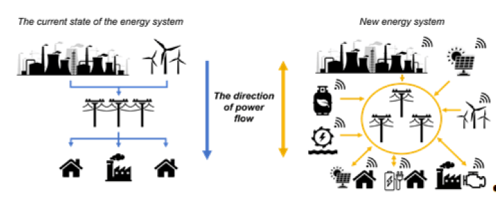
Contemporary LV power grids not only provide electricity to the end user, but are also designed to receive energy from local, prosumer distributed energy sources (DES) [1]. As the process of changing the paradigm of the operation of the LV distribution system has been quite rapid in its implementation, the distribution network has not adequately adapted to the new tasks. The new reality has created various technical problems. These problems include overvoltages, rapid voltage fluctuations, voltage harmonics, protection coordination problems and backflows of energy into the medium voltage grid. The presented issues result mainly from excess energy in local balancing areas. This phenomenon causes local voltage to increases in the network above the normative values Vn+10% [2]. The problem of the excessive voltage level in the LV grid can be solved by rebuilding the grid by using larger cable diameters with lower impedance and using shorter lengths of radial lines. This is a very expensive and time-consuming solution. In addition, investment costs are passed on to distribution system operators. Another solution to prevent the increase in voltage is the use of local, distributed energy storage (ES) systems (also in the form of electric vehicles) which would accumulate excess energy production from DES [3]. This is a solution more and more often considered by distribution network operators as well as the owners of installations with renewable energy sources (RES). In addition, the ES could return the stored energy during high demand for energy during peak system load hours. The costs of investing in ES facilities could be divided between distribution system operators, prosumers, and additional participants in the system services market. Another technical solution for the voltage regulation in the LV network is the use of transformers with taps where a step voltage regulation is possible. Most often it is a manual adjustment applied seasonally. This could already find solutions for automatic change of transformer taps, the socalled on-load tap changer for OLTC distribution transformers [4]. Hybrid transformer systems [5] as well as static compensators for voltage changes [6] can be used for smooth voltage regulation in the network. These solutions are not fully and commercially available and are currently considered only in scientific research. Nevertheless, these solutions provide great flexibility in regulating voltage changes in the LV grid. An interesting solution for voltage regulation in distribution networks is the so-called demand regulation [7]. The scientific literature describes many concepts of controlling the demand for electricity with the use of intelligent household appliances, electrical and thermal ES systems and other electrical devices.
This article will be a short review of selected methods of voltage regulation in a low-voltage distribution network, the changes of which are caused by variable or excessive generation of energy from renewable energy sources. Below there is discussion of the exemplary results of research on the ES system for voltage regulation with active and reactive power, which are the result of a project implemented jointly with the local energy distributor Enea Operator [8]. In the next chapter selected concepts of hybrid transformers and static voltage compensators will be presented. Exemplary results showing the possibilities of this type of system will be presented. The last topic will be voltage regulation by increasing the network load during high energy generation from RES. The presented results of the authors’ research will concern the concept of using intelligent home devices.
Energy storage
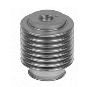
As part of the project [8], a prototype ES with a power of 100 kW and a capacity of 100 kWh, and in Valve Regulated Lead Acid (VRLA) technology (Fig. 1a) was created. This prototype was tested in both laboratory and real-life conditions. It was connected to the LV distribution network at the transformer station. The integration of the batteries with the LV distribution network was carried out using a power electronic converter made in the (SiC) technology. In the control of the power electronic converter, the algorithm for regulating the voltage of the power grid with the active and reactive power generated by the energy storage system has been implemented [9-12]. In the verification tests of the active and reactive power voltage control algorithm, voltage parameters in the power grid at the energy storage terminals were recorded. The power quality analyzer PQ-Box 150/200 for measurements was used. The results of voltage regulation for regulation both with and without active and reactive power were performed on the same day of the week (Fig. 1b). It is obvious that it is impossible to obtain identical operating conditions for the power system. Measuring voltage parameters on the same day of the week (presented results refer to Thursday) will give some approximation of comparable system operating conditions. Instantaneous network voltage values may exceed the set values which results from the dynamics of the control algorithm. There is a clear reduction in voltage fluctuations when the control algorithm is turned on [11]. In the power system without the regulation service turned on, the voltages reached values even above 250 V. The minimum voltages dropped to 238 V.

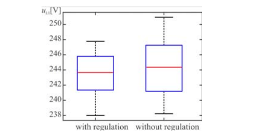
The details of changes in the grid voltage value are shown in the box plot in Fig. 2. A boxplot contains information about the location, dispersion, and shape of the data distribution. The box contains the first (Q1) and the third (Q3) quartiles. The points between the first and third quartiles represent 50% of the scores, and the median represents the middle of the scores. The median does not have to lie in the middle of the box. In addition, the minimum and maximum values are marked on the chart. The boxplot for the results with the compensation algorithm enabled indicates that the span between the voltage values was 238 V to 248 V. The span of the box, however, is 241.5 V to 245.8 V. The median was 243.5 V. For the results without compensation, the span the voltage results was from 238.2 V to 251.5 V and the box value was from 241.5 V to 247 V. The median was 244.1 volts. The presented results indicate the effectiveness of the applied voltage regulation with the use of energy storage.
Hybrid transformers and static voltage compensators
Another concept of voltage regulation in the network, compensation and voltage fluctuations is the use of hybrid transformers (HT) installed in a typical distribution station [5], [13] – [15]. The HT concepts are so far described in scientific articles as systems with high regulatory potential. They consist of an electromagnetic transformer that works with an AC/AC power electronic converter with PWM modulation. Fig. 3 shows single-phase implementations of two HT configuration concepts with a serial converter. In Fig. 3a, any AC/AC converter that regulates the root mean square (RMS) value of the voltage can be used as a power electronic converter. These can be frequency converters (back-to-back [5], matrix converter (MC) [14], [15]) or AC/AC voltage controllers [6], [13]. Fig. 3b also shows the scheme of the HT concept with a series power electronic converter with an additional battery energy storage. An additional DC energy storage is used to support the compensation process. An HT can be switched on anywhere in the power grid, but the most sensible solution is to replace classic substation transformers with the HT.


One of the HT concepts is the topology with the MC [14], [15]. Using the MC, it is possible to compensate for both symmetrical and asymmetrical voltage changes as well as harmonic distortions. It is also obvious that the grid voltage can be regulated in situations where the voltage is too high as a result of large generation of energy from RES.

The model predictive control (MPC) scheme for the proposed HT with MC is shown in Fig. 4. To illustrate the beneficial properties of the HT with the MC (Fig. 4), test results of the system are shown in Fig. 5. As can be seen in Fig. 5, the load voltage is kept at a constant amplitude without harmonic distortion, despite large variations in the main voltage. As already mentioned, voltage regulation can also be implemented using static compensators. Then it can be used anywhere on the power grid. An example of a selected AC voltage compensator topology using a bipolar AC chopper is shown in Fig. 6 [16]. These compensators have quite complex control strategies, but they can compensate for large voltage dips in one phase. In addition, they can be used to regulate long-term voltage and compensate for fast-changing voltage fluctuations. This article only shows the topology concept without analysing it in detail.

Energy management with smart home appliances
The concept of using and integrating smart home appliances (SHA) in the local low voltage balancing of the distribution grid in order to counteract the increase and decrease of voltage in the network is widely discussed in various scientific articles. Such concepts are still at the stage of theoretical consideration and prototype testing due to the lack of many household devices with free remote access to their regulation or activation. The emergence of the Internet of Things (IoT) technology may lead to a breakthrough in the use of home devices in regulating the load of the power system. Nevertheless, the first IoT applications in the SHA are focused on increasing the comfort and elasticity of using a given device. From the point of view of power system load regulation, the SHA should have the functionality of reacting to signals from the environment (remote control signals) and operating conditions – e.g., to the voltage level in the network. Therefore, the concept of a smart device suggests that smart devices not only perform their main functionality in a user-defined manner, but also autonomously respond to the environmental conditions in which they work.
Appropriate SHA control can bring the following benefits to the power system: balancing the supply of energy generated by RES to reduce transmission losses and thus increase the energy efficiency of the system; regulating the grid voltage and thus improving the reliability of the system and the devices operating in it; increasing the production from RES by not switching off the photovoltaic inverters under high voltage conditions in the power grid. It should be emphasized that to achieve these goals, the use of the SHA will require users to change their usage behaviour.
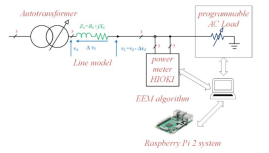
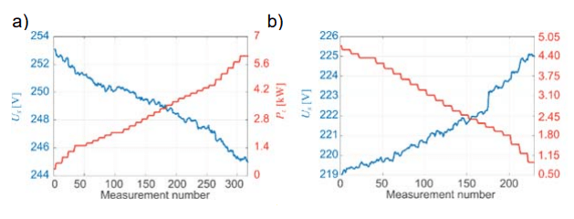
Works [17] – [19] propose to manage the work of the SHA through an algorithm called Elastic Energy Management (EEM). Various functionalities of the SHA operation were defined, which were controlled by an external signal from the central unit or based on the measurement of the voltage in the grid. These functionalities were related to limiting power consumption, pauses in operation or shifting the activation time [17]. All these functionalities have been saved in the EEM algorithm, where a database of devices and their ability to change power during operation should be created. The algorithm was implemented in the Raspberry PI device, which was controlled by a Programmable AC Load device (Fig. 7). During the test, the power was changed according with the settings and the number of simulated devices. The EEM algorithm changed the power of the devices until they reached the set limit of the mains voltage. Reaching the set voltage was associated with an increase (Fig. 8a) or decrease (Fig. 8b) in the grid load, which resulted in a change in the voltage drop on the line impedance.
While reducing the load on the line may be related to the shutdown of certain low-priority devices, increasing the load is not so simple. Devices must be defined that can be switched on freely or are prepared for operation in advance by the user [18]. The first group includes all battery devices (electric vehicles, laptops, tablets, telephones, etc.), whose chargers can be activated by an external signal. In addition, these can be water heating devices or ventilation and cooling devices. The second group consists of devices such as a washing machine, dishwasher, electric cooker. They are prepared by users for operation, and they can be activated by an external signal from the central control unit, which will send appropriate information about the RES generation. The use of the second group of home appliances will involve a change in the habits of users, as the activities can be permitted to be performed when the appropriate conditions for generating energy occur. It is obvious that the user will be able to freely change the settings of these devices so that their use corresponds to current needs. All work is focused on ensuring user comfort. In this case, the user has decisive roles. A decision may be made to switch the system to fully autonomous mode or manually. Some users will obviously use the autonomous mode most often, which will provide financial benefits (e.g., reduction of electricity bills). For a selected group of users, i.e., those with greater technological awareness, the manual or semi-manual mode will allow for better adjustment to their needs. Regardless of the target group of users, it would be required from the front-end side of the system to ensure that it was user friendly and responsive.
Conclusions
The article presents selected methods of the voltage regulation in the LV distribution network, the changes of which are caused by variable or excessive generation of energy from RES. There has been presented the discussion of exemplary results of the research on methods of the voltage regulation in a power grid with an ES system, HT and static voltage compensators, as well as by increasing the grid load during the production of large energy from RES with the use of smart home appliances.
The research results on a mature technological method of voltage regulation with the use of the ES are also presented. Voltage regulation can be achieved by controlling the active and reactive power generated by the power electronic converter connected to the ES. Similar results can be achieved by controlling the reactive power of solar inverters [19], or by using parallel reactive power compensators. The other proposals presented in the article are, for now, only scientific concepts. Nevertheless, it should be noted that the application of all three proposals could significantly improve the operation of the power system when too much energy is generated from RES. More detailed studies must be carried out considering the simultaneous operation of all the proposed methods.
Acknowledgments – Some of the results of this paper are part of projects that have received funding from the National Centre for Research and Development in the frame of the European Regional Development Fund (ERDF), program Smart Growth Operational Programme, action 1.2, project number: POIR.01.02.00-00-0232/16.
REFERENCES
[1] Benysek G., Kazmierkowski M.P., Popczyk J., Strzelecki R., Power electronic systems as a crucial part of Smart Grid infrastructure – a survey, Bulletin of the Polish Academy of Sciences: Technical Sciences, 59 (2011), No. 4, 455-473
[2] Hashemi S., Østergaard J., Methods and strategies for overvoltage prevention in low voltage distribution systems with PV, IET Renewable Power Generation, 11 (2017), 205-214
[3] Faisal M., Hannan M.A., Ker J., Hussain A., Mansor M.B., Blaabjerg F., Review of energy storage system technologies in microgrid applications: Issues and challenges, IEEE Access, 6 (2018), 35143-35164
[4] Aziz T., Ketjoy N., Enhancing PV penetration in LV networks using reactive power control and on load tap changer with existing transformers, IEEE Access, 6 (2018), 2683-2691
[5] Carreno A., Perez M., Baier C., Huang A., Rajendran S., Malinowski M., Configurations, Power Topologies and Applications of Hybrid Distribution Transformer, Energies, 14 (2021)
[6] Kaniewski J., Szcześniak P., Jarnut M., Benysek H., Hybrid voltage sag/swell compensators: a review of hybrid AC/AC converters, IEEE Industrial Electronics Magazine, 9 (2015), No. 4, 37-48
[7] Siano P., Demand response and smart grids – A survey, Renew. Sustain. Energy Rev, 30 (2014), 461-478
[8] https://www.gov.pl/web/ncbr/innowacyjne-uslugisystemowe-magazynow-energii
[9] Majumder R., Aspect of voltage stability and reactive power support in active distribution, IET Generation, Transmission & Distribution, 8 (2014), 442-450
[10] Zimann J.F., Batschauer A.L., Mezaroba M., Neves F.A.S., Energy storage system control algorithm for voltage regulation with active and reactive power injection in low-voltage distribution network, Electric Power Systems Research, 174 (2019), 105825
[11] Smoleński R., Szcześniak P., Drożdż W., Kasperski Ł., Advanced metering infrastructure and energy storage for location and ˙mitigation of power quality disturbances in the utility grid with high penetration of renewables, Renewable and Sustainable Energy Reviews, 157 (2022)
[12] Leżyński P., Szcześniak P., Waśkowicz B., Smoleński R., Drożdż W., Design and Implementation of a Fully Controllable Cyber-Physical System for Testing Energy Storage Systems, IEEE Access, 7 (2019), 47259-47272
[13] Kaniewski J., Fedyczak Z., Szcześniak P., Threephase hybrid transformer using matrix-chopper as an interface between two AC voltage sources, Archives of Electrical Engineering, 63 (2014), No. 2, 197-210
[14] Szcześniak P., A modelling of AC voltage stabilizer based on a hybrid transformer with matrix converter, Archives of Electrical Engineering, 66 (2017), No. 2, 371-382
[15] Szcześniak P., Tadra G., Kaniewski J., Fedyczak Z., Model predictive control algorithm of AC voltage stabilizer based on hybrid transformer with a matrix converter, Electric Power Systems Research, 170 (2019), 222-228
[16] Kaniewski J., Power flow controller based on bipolar direct PWM AC/AC converter operation with active load,. Archives of Electrical Engineering, 68 (2019), No. 2, 341-356
[17] Powroźnik P., Szcześniak P., Piotrowski K., Elastic energy management algorithm using IoT technology for devices with smart appliance functionality for applications in smart-grid, Energies, 15 (2022), No. 1
[18] Powroźnik P., Szcześniak P., Turchan K., Krysik M., Koropiecki I., Piotrowski K., An elastic energy management algorithm in a hierarchical control system with distributed control devices, Energies, 15 (2022), No. 13
[19] Chmielowiec K., Topolski Ł., Piszczek A., Hanzelka Z., Charakterystyki inwerterów fotowoltaicznych w świetle zapisów kodeksu sieciowego oraz wymagań polskich operatorów systemów dystrybucyjnych, Przegląd Elektrotechniczny, 97 (2021), No. 4, 81-87
Authors: dr hab. inż. Paweł Szcześniak, prof UZ, University of Zielona Góra, Institute of Automatic Control, Electronics and Electrical Engineering, Podgórna 50, 65-246 Zielona Góra, e-mail: p.szczesniak@iee.uz.zgora.pl; dr inż. Piotr Powroźnik, Uniwersity of Zielona Góra, Institute of Metrology, Electronics and Computer Science, Podgórna 50, 65-246 Zielona Góra, e-mail: p.powroznik@imei.uz.zgora.pl; mgr inż. Elżbieta Sztajmec, Rzeszów University of Technology, Departament of Power Electronics and Power Engineering, 35-959 Rzeszów, e-mail: e.sztajmec@prz.edu.pl.
Source & Publisher Item Identifier: PRZEGLĄD ELEKTROTECHNICZNY, ISSN 0033-2097, R. 99 NR 11/2023. doi:10.15199/48.2023.11.11