Electricity Transportation using HVDC Technology for Algerian Southern Sun Power Plants

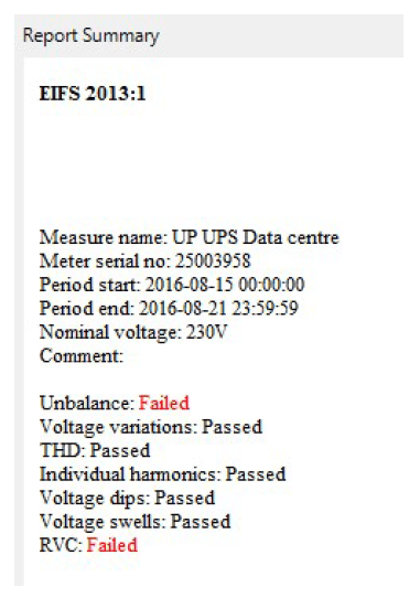
Published by 1. Mohammed SAAIDIA, 2. Abdelghani GUECHI, 3. Nedjem-Eddine BENCHOUIA, University Mohamed-Cherif Messaadia of Souk-Ahras . ORCID: 1. 0000-0002-7778-8591; 3. 0000-0002-4761-940


Abstract. Algeria is worldly known as one of the big producers and exporters of fossil fuels. However, by developing an adequate energy policy, it could become one of the great sun power (SP) producers and exporters. Indeed with almost 2 million Km2 sunny superficies, the country detains enormous SP energetic potential funds. However, eventual powerful SP plants deployment could be done far to the southern Algerian desert which makes HVDC technology the best candidate for the transmission of produced electricity towards the north region where are the main industrial poles and the most populated regions for local consumption and eventually farther to the north for electricity exportation to the European countries. The prospection work presented hereafter is a study on the feasibility of using HVDC technology for such possible projects according to country’s existing means and topographical and environmental characteristics.

Streszczenie. Algieria jest znana na całym świecie jako jeden z największych producentów i eksporterów paliw kopalnych. Jednak opracowując odpowiednią politykę energetyczną mogłaby stać się jednym z wielkich producentów i eksporterów energii słonecznej (SP). Rzeczywiście, z prawie 2 milionami km2 słonecznych powierzchni, kraj ten posiada ogromny potencjał energetyczny SP. Jednak ewentualne rozmieszczenie potężnych elektrowni SP mogłoby zostać przeprowadzone daleko na pustyni południowej Algierii, co sprawia, że technologia HVDC jest najlepszym kandydatem do przesyłu wyprodukowanej energii elektrycznej w kierunku regionu północnego, gdzie znajdują się główne bieguny przemysłowe i najbardziej zaludnione regiony do konsumpcji lokalnej i ostatecznie dalej na północ w celu eksportu energii elektrycznej do krajów europejskich. Przedstawione poniżej prace poszukiwawcze są studium wykonalności wykorzystania technologii HVDC do takich możliwych projektów, zgodnie z istniejącymi środkami kraju oraz charakterystyką topograficzną i środowiskową. (Transport energii elektrycznej z wykorzystaniem technologii HVDC dla południowych elektrowni słonecznych w Algierii)

Keywords: HVDC; electrical power transport; sun power; photovoltaic.
Słowa kluczowe: HVDC; przesył energii elektrycznej; moc słoneczna; fotowoltaika.

Introduction

Electricity power production-consumption industry is largely dependent on the transportation process. Indeed, its importance is directly related to the quality of the delivered electricity, the quality of distribution services, the unitary prices and moreover to some environmental concerns. HVAC (High Voltage Alternative Current) was, for a long time, the mostly used technology for electricity power transportation. This was mainly due to the alternative nature of the produced electricity and also to economical raisons. However, technological advancements, electrical power networks developments and emergent electrical power sources have bring to the fore the HVDC (High Voltage Direct Current) old technology as a competing and alternative technology.

Thanks to decades of active research efforts and huge investments, HVDC (high voltage direct current) technology had become a real and practical alternative to HVAC one. The line cost per Km rapidly became in favor of this new alternative over long distances electrical transportation lines (several hundreds of Km) and for powers beyond 200 MWs. Practical financial studies demonstrate that HVDC losses still around only 3% for 1000 Km overhead lines connection [1] . Moreover, gains in used cables (about 50%) as well as huge reduction in the cost of cable supports make the HVDC technology more suitable according to environmental point of view as well as economically. These facts make HVDC systems the most electrical power transportation mean for powerful electrical interconnections between countries and even more between continents. It also happens that this type of electricity technology is more suitable for certain forms of renewable energies like photo-voltaic (PV) energy since the latter is directly produced in DC form [1], [2].

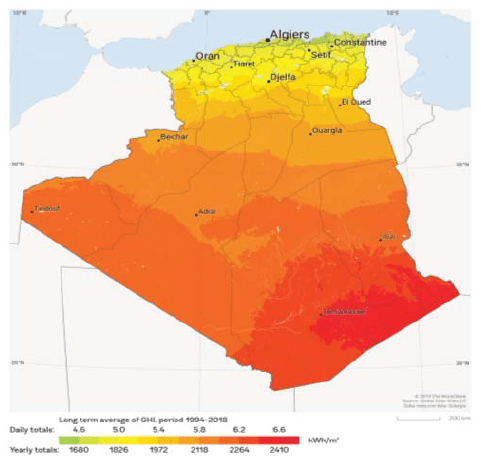
Thanks to its highly sunny 80% of its superficies (about 2 million Km2), Algeria registers one of the worldwide highest sunshine duration from 2,000 to 6,000 Wh/m2 according to regions. This enormous solar power potential could permit a very high production of clean SP energy which is far exceeding its consumption and could makes the country an eventual exporter of this type of highly coveted energy. However, like it’s demonstrated on the map of figure 1, the most sunny sites for possible mass production of this type of energy are far to the south; which makes HVDC electricity transportation technology a suitable candidate in the case of the country and encourages its adoption.

Fig.1. Algerian sunny power distribution zones (kWh/m2)

During last decades, researchers, in the HVDC field, were very active and were mainly focused on electronic parts of HVDC systems, especially converters and inverters, the exploitation of SP energy in HVDC form for everyday applications and of course the DC electric power transportation.

This investigating work begin with an overview of the basic notions of the HVDC electrical power transportation system, then a detailed environmental and economic study of the advantages of using HVDC according to the different strategic characteristics of the country is presented. Finally, this study is concluded by highlighting the key-basis of a possible real implementation of the HVDC solution.

HVDC basic notions and importance

By nowadays, HVDC technology has reached high level performances in its different components such as electronic parts, cable characteristics, pylons specifications and management capabilities. These advancements are results of research efforts, laboratory investigations and practical projects deployments. In the following subsections we will detail the principal and fundamental basis of HVDC.

Basic notions on HVDC

Despite the fact that AC technology dominated and still dominating the electrical engineering from the production process to the consumption going through the transport and distribution intermediate operations, the HVDC technology appears to be on the right way to regain one’s share of the market. At the production stage, some of the renewable energy resources like PV systems give DC currents instead of AC ones. The electrical power transportation also have seen the deployment of HVDC electrical networks especially in cases of powerful long distances transport requirements. This welcomed comeback of HVDC was supported essentially by research and applications on DC electricity, semiconductor technology and control theory. This comeback was aided by 7 principal advantages versatile the AC configuration namely [3];

• Low financial investment
• Lower losses for bulk power transmission
• Capability to interconnect asynchronous grids
• More efficiency for underground and submarine transportation
• Improve performances of parallel transmission for AC circuits
• Better controllability since it permits an instant and precise power flow control
• For an equivalent ROW, DC provides 3 times more power than AC.

Moreover, advanced HVDC configurations permit also more advantages namely;
• Costs are close to overhead lines
• Possibility to connect passive loads
• Useful for enhancement of connected AC networks
• Active and reactive power are controlled independently
Reduced delivery times for HVDC projects.

HVDC projects’ deployment

HVDC electrical power transport technology has been, for a long time, used in a limited manner for some important projects. The investments in these projects helped to experiment the new invented technologies and rise the met challenges. Nowadays, HVDC systems become so competitive that under certain conditions it overcomes the HVAC technology which permits an important deployment of HVDC systems. Figure 2 gives a graphical HVDC projects’ spread in different parts of the world.

The globalization of electricity power transportation permits networks interconnections between countries and continents. This new trend imposed the construction of electric transportation lines on long distances and with huge power; which makes HVDC the essential solution to be adopted [4][5].

In Algeria, HVAC is the exclusive technology that is used from the production till the consumption. The availability of oil and gas fuel resources permitted to the exclusive producer of electricity (SONELGAZ) to adopt the simplest strategy based on the construction of production stations close to the consumer which makes the transport of electricity limited to short distances [6].

Fig.2. World’s projects deployment of HVDC electrical power transmission

Fig.3. Algerian electricity production and transmission network deployment Source: SONELGAZ

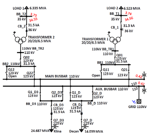
Figure 3 gives an overview of the topology of the electricity production stations and transmission lines of the Algerian network deployment. The production stations goes from 220KV (red circles) down to 60KV (green circles). The transportation lines use the same color codification (red for 220KV and green for 60KV) [7], [8].

However, new development trends tend to change the course of this industry. The following Algerian specificities could drive such a trend:

– Emergence of renewable energies and especially sun power production technologies. – Enormous sun power potentials

– Large sunny areas (more than 2 Million Km2) – Most sunny southern regions are far from populated and industrialized poles (the Sahara)

– Country’s propitious financial situation which could help to put sufficient investments to achieve promising goals

– Country economic strategy aspiring to impose it as a major exporter of renewable electricity, especially towards Europe

Technologists, economists, and even politicians are all aware of energy issues in the coming decades. Renewable energies became not only a trend subject of discussions for different interested actors in Algeria but a real challenge that has to be met. The Algerian electricity and gas company (SONELGAZ), exclusive producer and distributor of electricity in Algeria, had already taken practical steps towards the new renewable energies era. Indeed, SONELGAZ has created a subsidiary which deals with the production of renewable electricity especially PV one. Plans and schedules are ongoing to attain important renewable electrical power production not only for local consumption but also exportation. However, important production stations will be spread far to the south where the most important irradiation rates are recorded. To support this trend, HVDC technology could be deployed according to economic and environmental studies.

Environmental and Economic Aspects

Renewable energies resources are found to be potentially sufficient to respond to the humanity growing energy demand while remaining respectful of the environmental protective policies. Solar energy plants and offshore wind pharms are best examples of such energy resources. However, these resources of energy are located in areas far removed from populated regions and the transmission of the enormous electrical energy is carried out over long distances (Fig. 4).

Fig.4. Algerian classical electrical power production and transport network. Source: Global Energy Network Institute (2017)

To solve this problem, the use of HVDC technology is one of the solutions that can help to provide power from these areas. Therefore, new trends to attain a more sustainable world will give the HVDC technology an important role in this way of development. In addition, the new HVDC technology enhancements like VSC, MTC and MMC technologies appear to be economically good alternatives for the future extensions of the transmission networks across the planet.

Power transmission efficiency, economic benefits, technical concerns and environmental issues are the main supports of the HVDC technology.

Environmental advantages of HVDC

• Visual impact and space requirements:

The efficiency of HVDC transportation technology permits more efficient exploitation of existing standard power plants and even new renewable energy ones. This fact will lead to minimize power losses and to improve earth’s exploitation resources which are important parameters to measure the environmental-friendly of any technology [9].

In HVAC electrical power transportation, the over-head transportation trough cables and tower’s is the main mean which is used at 90% of cases since it’s technologically and economically the most efficient mean. HVDC technology offers more alternatives. In HVDC transportation technology the three known transportation means; namely over-head, underground and underwater; could be used alternatively according to environmental topographical characteristics. For over-head transportation mean the tower’s visual impact is therefore reduced to only converter stations comparatively to the case of HVAC [9] [10].

From visual impact point of view and for a comparable power transmission capacity, HVDC overhead transmission lines have less intrusive environmental effect. Example given could be the case of Bipolar HVDC transmission lines which have two conductors and already because of that are simpler in design in comparison with the three-phase structure of a HVAC line of the same capacity and comparable voltage levels. In this case, shorter tower heights are used for HVDC technology which affects environmental and economic parameters [11].

Another exemplar case would be the case when quadric-polar HVDC lines are used for power transmission. Here, flat towers or towers with two cross-arms, according to transmission corridor’s conditions, will be used. For a ±500 kV HVDC transmission line, Figure 5 gives schematic views of these tower types. Approximate tower dimensions are indicated. According to the specificities of the constructed transmission line, a choice of tower design would be done. However, for any case, the dimensions of the towers for the HVDC quadric-polar line are smaller than those used for a double-circuit HVAC line with comparable capacity [11]. Moreover, the width of corridors opened for the electrical line transmission are consequently reduced (about 1/3) in case of HVDC technology compared to HVAC one. Given a line with the same capacity (500KV for example), the corridor for an HVDC connection will be 55m to 60m; however it will need a corridor of 65m to 70m in case of an HVAC double circuit or a corridor of 105m in case of an HVAC single circuit [12].

Fig.5. Schematic of two tower’s variants (flat and two cross-arms) used for ±500 kV quadric-polar HVDC transmission line

Moreover, HVDC technology offers superior performances and capabilities when using underground or underwater connections. For underground connections, they will be considered as exclusive for HVDC since for HVAC they will require large tranches to avoid interactivity between the three phase’s cables.

In the case of HVDC, tranches about only 50cm to 80cm large and 1m to 1.5m of deepness are sufficient to contain bipolar electrical transmission line with a power transmission of about 1200 MW. According to an environmental point of view, narrow tranches are the friendliest means for such transmission lines. In the case of submarine transmission lines and over 50 Km, the use of HVDC technology becomes inevitable. Studies demonstrate no consequent effects of established submarine transmission lines on submarine’s life. Furthermore, installed cables do not need any maintenance or servicing operations during their lifetime (except in force majeure cases) which permits their integration to their surrounding environment.

All these environmental specificities could be applied to topographic characteristics of Algerian lands. Indeed, combining information on figure 1 and figure 4, we can easily see that the sunniest areas that already contain infrastructural facilities are the regions of Bechar, at the west, Gardaia, at the center, and Hassi-Messaoud at the east. These areas are at least 700 Km to 800 Km far from the most populated and industrialized northern zones of the country. Added to this, 70% of this distance is flat and uninhabited lands (Desert). Most of the remaining 30% distance are mountainous lands. In the case of electrical power exportation towards Europe, distances could go over a 1000 Km with some hundreds of Km in the Mediterranean Sea.

• Electric and magnetic fields: A well-known physical effects produced by conducting electricity in cables are electric and magnetic fields. These two effects were well studied and efficiently measured. For an HVDC over-head transmission line, for example, the electric field is due to firstly the potential difference between the electrical conductor and the earth and secondly to the space charge clouds that are due to Corona effect in the conductor [13].

As a natural effect, the Electrostatic fields are spread through the global atmosphere but they became stronger around electrical conductors. As this, human bodies are adapted to this type of physical effects but when they still at acceptable natural ranges. However, out of natural ranges values, they will become an ecological and even biological concern for human beings like possible shock hazards [14]. Combination of the electrostatic field and the space charge field creates the electrical field generated by an HVDC transportation line. Fortunately and in the way, the conductors of the HVDC transmission line in corona generate ions of the same polarity as the conductor itself which are drifted either to the ground or to a conductor of opposite polarity.

Measurements of the electrical field distribution at ground level under HVDC electrical line transmission demonstrate that it depends on the distribution of space charges between the conductors and the ground. The presence of space charge with the same polarity as the conductor increases the electrical field at the ground level but those with opposite polarity decreases it [14]. This fact, encourages the use of bipolar and even quadric-polar HVDC line transmissions instead of mono-polar ones since the presence of conductors of opposite polarities will decreases the global density of the electrical field at the ground level.

Table 1. Examples of natural and artificial sources of electric and magnetic fields

.

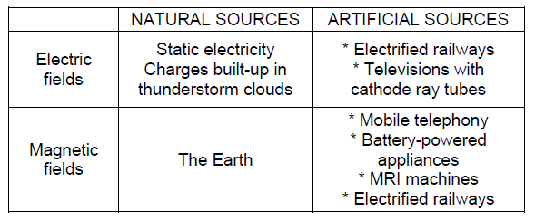
In the same way and for environmental and biological concerns for the human body, the magnetic field associated with an HVDC transmission line was studied. Studies demonstrate that magnetic field had no noticeable effects on the human body. In a counterpart, this physical phenomenon has important influences on certain types of human machines. The well-known case is the disturbances that were measured for the magnetic compass systems mounted on vessels when they became close to an undersea HVDC transmission line [9][10].

• Radio/TV interference:

Here also for radio interference caused by electric power transmission lines, HVDC technology still preferred to HVAC technology. This is due to the fact that for HVDC conductors the result of the corona discharge around them is generated only by conductors of positive polarity hence they are those who generate radio interferences. This encourages the use of bipolar and even quadric-polar HVDC transmission lines which permits an important increase of the transported power without increasing interferences. This could not be applied to HVAC transmission technology since all the transmission conductors are sources of interferences and increasing the number of conductors would imperatively increase these interferences.

Radio frequency perturbations produced by electrical transmission conductors are also subject to weather conditions. Indeed, rainy weather affects the HVDC and HVAC transmission conductors differently since it causes an increase of about 10 dB of radio interference generated by conductors of an HVAC line transmission. However, for conductors of an HVDC line the radio interference decreases considerably under condition of providing a surface voltage gradient of 25kV/cm.

In normal conditions and for an equal capacity transportation of conductors and maximum levels of electrical field intensity on their surfaces, the radio interference level of HVDC lines is typically lower by 6-8 dB than of HVAC lines [11].

However, for HVDC transmission line, converters’ switching modes cause disturbances in the kHz and MHz regions of interference. The main solution to this problem was the introduction of an appropriate shielding of valves which minimizes the amount of these disturbances and makes the radio interference of the HVDC line comparable with AC solutions [15].

• Audible noise:

Audible noise is an easily perceptible problem by each human body. Thus it’s with great concern that designers of electrical transmission lines deal with the control parameters of such a problem for both overhead lines and substations. However, used means to decrease audible noise of these electrical sources are quite costly. As a standard rule, the audible noise from transmission lines should not exceed, in residential areas, 50 dB during the day, or 40 dB at night.

For HVDC systems, the principal sources of audible noises are the substations and the transmission conductors. The substations contain converter-transformers which are the main sources of audible noises. These devices are generally surrounded by screens which provide an efficient limitation of the noise levels that outgo the substations and pollute the environment. On the other side, the transmission lines produce broadband noises which pollute noises extent to high frequencies. Electrical line transmission noise is most prevalent in fair weather. Audible noise levels produced by conductors of HVDC line usually decrease during foul weather which is completely the opposite state for the AC transmission lines for which it increases considerably.

In the case of underground and submarine HVDC transmission lines, no audible noise is perceptible. The main issue rises for the over-head transmission lines during foggy weather.

Consequently, restrictions are imposed on the construction of buildings at the closest areas of a transmission lines and their substations. Studies and measurement demonstrate that audible noise is directly related to line’s voltages levels, technical line’s specifications and the climatic state of the regions crossed by the electrical transmission line [16].

Economic benefits of HVDC

Despite the notorious environmental effects already exposed, the practical implementation of any technological solution (HVDC in this case) is directly linked to the economic parameters and advantages it presents.

As it’s depicted in Figure 6, the establishment of any electric transmission line, in HVDC or HVAC technology, induces costs mainly related to the materials used (cables, towers, electronics), to engineering works (actual installation) and to preparation works (civil works). Other expenses of lesser amounts are also expected including investigation work as well as insurance on the works and on the line.

Fig.6. Distribution of Costs in percentage related to different types of works and services

We present hereafter economic comparatives between comparable transmission lines in HVDC and HVAC technologies.

• Used materials:

Electronics are the most applied costs in the installation of an electrical transmission line (about 63%). Compared to terminal stations of an HVAC connection, terminal converter stations on the two ends of an HVDC electrical transmission line costs much more. However, HVAC connections on long distances increase mutual inductances and capacitances that are related to the nature of the alternative current. These two phenomenon added to losses on the long distances line impose the construction of intermediate switching stations for voltages levels maintain and reactive power compensation. Figure 7 gives an approximate partition of the line cost between the terminal stations’ expenses and the rest of the realization works for both HVDC and HVAC technologies [17].

Fig.7. Partition of line cost between terminal stations realization and other works for both HVDC and HVAC technologies

The Figure 7 also demonstrates that by increasing the line connection distance, the advantage balance goes in favor of the HVDC connection technology [18]. What is exactly the distance from what we opt for HVDC technology depends on several parameters. This distance is called “Break-even distance”.

Cables that are used for electricity transmission are also an important parameter that weights in balance. Indeed, HVDC technology uses much more technological developed cables which means much more expensive but fortunately, the quantity of cables for a comparable HVDC transmission line is reduced at least by the third compared to HVAC one. At the beginning of HVDC transmission line projects, mono polar connections were used. However, newly installed projects are using bipolar transmission lines since for same number cables we can double the transmitted power.

Towers that support cables have more reduced structure in HVDC transmission lines which makes them less high with less weight and consequently much cheaper than those used for HVAC technology [11].

• Engineering works:

Engineering works encompass all technical operations related to the installation of terminal converter stations, the passage of the cables and realization of the necessary tests and verification of the validity of the connection. It represents 10% of the total cost of the transmission line which is a lot.

HVDC transmission lines installation requires that technical staff has to be more specialized since on one hand the electronics technologies involved in this type of installation are the newest and on another hand each new HVDC transmission line is characterized by each own specific technologies like for the types of cables, the valves configurations and so on. This involves more expenses compared to an HVAC transmission line which technologies have already attained its maturity long time ago. However, these supplementary costs are compensated by the reduced works that are required for an HVDC line compared to an HVAC one. Here also the “Break-even distance” has to be determined for a given electrical transmission line.

• Engineering civil works:

Civil works are an important part of the electrical transmission line realization. With an amount of about 14% of the global amount of the whole realization cost of the transmission line, civil works represents the second portion of expenses. Civil works encompass the route study and optimization, the installation of towers for over-head connections, the digging of tranches and their fitting out for underground parts of the line and even works on the seabed for underwater connections. The preliminary study determines the type of connection adapted to each type of terrain such as plains, plateaus, mountains, lakes and seas

Fig.8. HVDC and HVAC electrical line costs according to the transmission distance

The study of the overall cost of an electrical transmission line determines a comparison between realization costs using HVDC and HVAC technologies. A general rule called “Break-even distance”, illustrated on Figure 8, is often used to prevail one over the other [17].

In addition to economic reasons, technical ones are also important to make balance between HVDC and HVAC technologies. Indeed, HVDC technology is well known for providing a practical stability improvement of the network and could make connection between HVAC networks with different operating frequencies.

Current situation and finalized projects

Despite the fact that Algeria is an oil producer country, it is easy to see the political, economic and even public awareness of global energy issues. This awareness is manifested by the fact that everyone knows the importance of new forms of so-called renewable energy production. Even on a public scale, people are ready to embrace the integration of these energies into everyday life. At a larger scale, successive government plans attempt to fit into global efforts in this area. Thus, over the past 15 years there have been some successfully realized projects.

Table 2 and figure 9 give an overview of these projects, some information about each one and their locations on the country territory.

Table 2. Algerian sun power stations and their capacities

.
Fig.9. Algerian Sun power stations localization

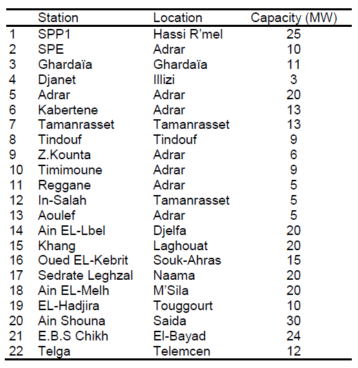
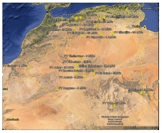
We can see that 10 of the 22 stations are allocated far to the middle and the borders of the Algerian Sahara. Figure 10 gives images of two types of SP power stations, one PV station at the North (Oued-Elkebrit) [19] and one CSP station at the south (Adrar)

Fig.10. PV station at Oued-Elkebrit and CSP station at Adrar

Moreover, all Algerian governmental plans are aspiring to bring Algeria from the status of “oil producer and exporter” to “sun power producer and exporter”. In 2019 Algeria had 21.2 GW of electricity installed generating capacity among which only 305 MW were sun power production. According to these plans, the Algerian renewable energy power production could attain 22 GW by 2030. All plans are axed on the realization of centralized SP mega stations (PV and CSP stations) at the regions of Bechar, Timimoun, Gardaia and Hassi-Messaoud. The mean distance from these regions to the northern populated and industrialized zones is about 800 Km which could inevitably enforce the HVDC transportation solution as the best mean for the electrical network interconnection.

Conclusion

The presented study was dedicated to investigate the environmental and economic characteristics of Algeria that permits to deploy an HVDC electrical power transportation network. Firstly, the principle characteristics of HVDC technology were presented and justified. Afterwards, each environmental and economic parameter was studied according to the specificities of the country. For each studied parameter we find that it was propitious to the use of such technology and could be a favorable support to its implementation. At last, the state of the situation in Algeria was presented and expectations also.

REFERENCES

[1] Abhisek Ukil, “Frequency converter based tuned high voltage AC transmission: Design and Implementation Issues”, Region 10 Conference (TENCON) 2016 IEEE, pp. 713-717, 2016.
[2] P.A Gbadega, A. K. Saha, “Loss Study of LCC-Based HVDC Thyristor Valves and Converter Transformers Using IEC 61803 Std. and Component Datasheet Parameters”, PES/IAS PowerAfrica 2018 IEEE, pp. 32-37, 2018.
[3] G.w. Juette ; H. Charbonneau ; H.i. Dobson ; C. Gary ; N. Kolcio ; M. Moreau ; J. Reichman ; E.r. Taylor”CIGRE/IEEE Survey on Extra High Voltage Transmission Line Noise”, IEEE Transactions on Power Apparatus and Systems, vol. PAS-92, pp. 1019-1028, May/June 1970.
[4] Chijioke Joe-Uzuegbu ; Gloria Chukwudebe, “High Voltage Direct Current (HVDC) technology: An alternative means of power transmission”, 3rd IEEE International Conference on Adaptive Science and Technology (ICAST 2011), Nov. 2011, Abuja, Nigeria
[5] Roger Wiget, Göran Andersson, “DC optimal power flow including HVDC grids”, Electrical Power & Energy Conference (EPEC) 2013 IEEE, pp. 1-6, 2013
[6] Herbadji, Ouafa; Slimani, Linda; Bouktir, Tarek, “Solving Bi-Objective Optimal Power Flow using Hybrid method of Biogeography-Based Optimization and Differential Evolution Algorithm: A case study of the Algerian Electrical Network.”, Journal of Electrical Systems . 2016, Vol. 12 Issue 1, p197-215
[7] Ahmed SALHI, Djemai NAIMI, Tarek BOUKTIR, “Fuzzy Multi- Objective Optimal Power Flow Using Genetic Algorithms Applied to Algerian Electrical Network », Journal of Power Engineering and Electrical Engineering, VOL. 11, Issue 6, December 2013
[8] Abdelkader Harrouz ; Meriem Abbes ; Ilhami Colak ; Korhan Kayisli, “Smart grid and renewable energy in Algeria”, 2017 IEEE 6th International Conference on Renewable Energy Research and Applications (ICRERA), November, 2017, San Diego, CA, USA
[9] SEIMENS. High voltage direct current transmission – proven technology for power exchange. brochure from SIEMENS, March 2007, Available online: http://www.siemens.com, 2007.
[10] J. Setrieus and L. Bertling. “Introduction to HVDC technology for reliable electrical power systems”, 10th IEEE International Conference on Probabilistic Methods Applied to Power Systems, pages 1–8, 2008
[11] P.F. de Toledo, “Feasibility of HVDC for city infeed. Thesis for the degree of Licentiate”, Department of Electrical Engineering, KTH, Stockholm, Sweden, 2003
[12] H. Acaroğlu , A. Najafı , Ö. Kara and B. Yürük , “An economic and tchnical review for the utilization of HVDC in Turkey and in the world “, Konya Mühendislik Bilimleri Dergisi, vol. 9, no. 3, pp. 811, Sep. 2021, doi:10.36306/konjes.907309.
[13] Palo Alto, “EPRI: Electrical Effects of HVDC Transmission Lines – State of the science”, CA: EPRI, 2010
[14] PS Maruvada, R D Dallaire, OC Norris-Elye, CV Thio, and JS Goodman, “Environmental effects of the Nelson river HVDC transmission lines – RI, AN, electric field, induced voltage, and ion current distribution test”, IEEE Transactions on Power Apparatus and Systems, Vol. PAS-101, No. 4, April 1982
[15] J. Paulinder; “Operation and control of HVDC links embedded in AC systems”, Thesis for the degree of Licentiate, Chalmers University of Technology, Gothenburg, Sweden, 2003
[16] D. Ravemark and B. Normark, “Light and invisible; Underground transmission with HVDC Light’, ABB, ABB Review, pages 25–29, 2005
[17] B.R. ANDERSEN, “HVDC transmission-opportunities and challenges. AC and DC Power Transmission”, ACDC 2006. The 8th IEE International Conference on, vol., no., pp. 24- 29, 28-31 March 2006
[18] M.P. Bahrman and B.K. Johnson, “The ABCs of HVDC transmission technologies”, IEEE Power and Energy Magazine, 5(2):32–44, 2007
[19] M. Saaidia, T. Belhouchat, N. -E. Benchouia and K. Achibi, “One day ahead prediction of PV power production: case study of Oued-Elkebrit’s station (Algeria),” 2019 1st International Conference on Sustainable Renewable Energy Systems and Applications (ICSRESA), Tebessa, Algeria, 2019, pp. 1-8, doi: 10.1109/ICSRESA49121.2019.9182702.


Authors: dr. Mohammed SAAIDIA, Dpt. of Electrical engineering, University of Souk-Ahras, P.O Box 1553, Souk-Ahras, 41000, Algeria, E-mail: mohamed.saaidia@univ-soukahras.dz; Abdelghani GUECHI, Dpt. of Mechanical engineering, University of Souk-Ahras, P.O Box 1553, Souk-Ahras, 41000, Algeria, E-mail: guechia123@gmail.com; prof. dr. Nedjem-Eddine BENCHOUIA, Dpt. of Mechanical engineering, University of Souk-Ahras, P.O Box 1553, Souk-Ahras, 41000, Algeria, E-mail: n.benchouia@univsoukahras.dz


Source & Publisher Item Identifier: PRZEGLĄD ELEKTROTECHNICZNY, ISSN 0033-2097, R. 99 NR 8/2023. doi:10.15199/48.2023.08.7

Determination of the Place and Degree of Damage Insulation in Cables

Published by Nahid MUFIDZADA1, Gulgaz İSMAYILOVA2, Azerbaijan State Oil and Industry University, Power Faculty, “Electroenergetics” department, Baku, Azerbaijan
ORCID: 0000-0003-4063-2128, 0000-0003-0063-2020


Abstract. A new method has been developed to determine the location and degree of insulation damage in cables. An electrical circuit is defined, using which this task is performed. According to this scheme, one end of the cable is connected to a pulsed voltage source through a small resistance, and the other end is grounded through a resistance equal to its wave impedance. By measuring the voltages at the beginning and at the end of the cable, curves are drawn depending on the ratio of voltages at the end and at the beginning of the cable from the distance between the point of damage and the beginning of the cable, with various degrees of damage to the insulation in it. Using the curves of this dependence α=f(x/l), the location and degree of insulation damage in cables is determined.

Streszczenie. Opracowano nową metodę określania miejsca i stopnia uszkodzenia izolacji w kablach. Definiowany jest obwód elektryczny, za pomocą którego wykonywane jest to zadanie. Zgodnie z tym schematem jeden koniec kabla jest podłączony do pulsującego źródła napięcia przez mały opór, a drugi koniec jest uziemiony przez opór równy jego impedancji falowej. Mierząc napięcia na początku i na końcu kabla, rysuje się krzywe w zależności od stosunku napięć na końcu i na początku kabla z odległości pomiędzy miejscem uszkodzenia a początkiem kabla, przy różne stopnie uszkodzenia izolacji w nim. Korzystając z krzywych tej zależności α=f(x/l) określa się miejsce i stopień uszkodzenia izolacji w kablach. (Określenie miejsca i stopnia uszkodzenia izolacji w kablach)

Keywords: Cable, insulation, degree of insulation damage, impulse voltage.
Słowa kluczowe: Kabel, izolacja, stopień uszkodzenia izolacji, napięcie udarowe

Introduction

Increased requirements are imposed on the reliability of cable lines and, consequently, on their insulation, since a lot of time and money are spent on finding the place of damage and, especially, on eliminating it in underground lines.

Causes of defects in cables are very diverse. Defects appear mainly in the weakest elements of cable insulation in the form of air inclusions, in which such dangerous processes as ionization and partial discharges develop. Determining the location and degree of damage in a cable line is a very important task, the relevance of which is currently confirmed by numerous studies by scientists from different countries [1,2,3,4].

Carrying out preventive tests can not always accurately determine the nature of the malfunction, and in some cases may not determine the presence of damage at all. Tests can only determine the presence of a fault in cables if its insulation level is reduced by at least 80 – 90% [5]. At the moments of an accident, cables often receive secondary damage. By type, such damage is divided into short circuits (in networks with isolated neutral) and breaks [6].

To determine the distance from the end of the cable to the point of damage in case of wire breaks and interphase and single-phase short circuits, the impulse research method is widely used [2,4].

The inevitable material and financial losses caused by the failure of the cable line (CL) force us to look for the most effective and minimizing these losses ways to eliminate damage. The correct choice of the method and equipment for searching for damage sites determines the quality of the solution to the problem, i.e. the maximum probability of correctly determining the location of the damage and the minimum time spent on this [8].

Analysis and purpose of the work

The presented article provides a method that can also be called a pulse method for determining the location and degree of cable damage. The determination of the location and the degree of damage to the insulation, as well as the location of the phase wire break during impulse effects on the cable, are considered. To do this, a pulsed voltage is applied to the cable input, which can be used as a pulsed standard wave of 1.2/50 μs of small amplitude through a sufficiently small resistance so that the cable input does not have a constant voltage equal to the applied voltage, and also be able to measure the current in that part. The end of the cable should also be grounded through a resistance to measure current and voltage in this part of the cable. In order to avoid the influence of the reflected wave at the end of the cable, the values of this resistance should be taken equal to the characteristic impedance of the cable. Otherwise, there will be two points in the cable (the point of insulation damage and the end of the cable), at which reflection and refraction of the wave will occur, leading to the complication of the wave process in the damaged cable. The design scheme is shown in Figure 1.

Fig.1. Design scheme

In the study, a cable with paper insulation and viscous impregnation was used, with a cross section of 120 mm2 with a rated voltage of 35 kV [8]. The length of the cable was assumed to be 1000 m. The study can be applied to metal cables of all types.

In calculations, the cable is represented by a traditional equivalent circuit in the form of a chain consisting of 30 elements.

Insulation damage and phase wire breaks were considered separately at 15 points located at distances of 0.067∙n from the beginning of the cable, where n are the numbers of these 15 points, 0.067 is the relative length between two adjacent sections. Determinations of the degree of insulation damage were carried out for cases of insulation damage of 30, 50, 60, 70, 80, 90, 95 and 100 percent.

Results and Discussion

The calculations were carried out using the algorithmic language OrCAD-17.

The results of calculations for determining the location and degree of insulation damage are shown in Table 1 and in Figure 2 – 5.

As can be seen from Table 1, regardless of the degree of damage to the insulation and its location in the cable, there is a slight change in the voltage values in the section (0 – 0.4) l of the cable, and in the section (0.4 – 1.0) l the voltage does not change. The deterioration of the insulation affects the voltage at the beginning of the cable, only for faults very close to the beginning of the cable.

As for the voltage at the end of the cable, this voltage along the cable varies in a very narrow limit for each value of the degree of damage, but with an increase in the degree of damage, starting from a value of 80%, this voltage decreases ( Table 1).

To generalize the obtained results, the dependence of the voltage ratio at the end and at the beginning of the cable (𝛼 = 𝑈к / 𝑈nom) on the distance of the damage point from the beginning of the cable, i.e. dependence α = f(𝑥/l). This dependence for all considered degrees of insulation damage, except for 100% damage, is shown in Figure 2.

Fig.2. Dependence of the ratio of stresses at the end and at the beginning cable from the distance of the fault from the beginning of the cable.

At 100% insulation failure, the remaining part of the cable between its end and the damaged point is short-circuited at the fault, and therefore the current and voltage in the shorted part of the cable become zero.

In Figure 2, curves – 1, 2, 3, 4, 5, 6 and 7 refer to the degrees of damage respectively 30, 50, 60, 70, 80, 90 and 95 percent.

As an example, Figure 3 shows the voltage curve at the beginning and at the end of the cable with a degree of damage to its insulation of 90% in the middle of the cable.

According to Figure 2, determination of the degree of insulation damage and its place in the cable is possible if the insulating properties of the cable are reduced by at least 80% (curves – 1, 4 and 7). At lower degrees of insulation damage, the corresponding curves are located very close to each other, which makes it impossible to determine either the degree of insulation damage or its place in the cable.

According to Figure 2, determination of the degree of insulation damage and its place in the cable is possible if the insulating properties of the cable are reduced by at least 80% (curves – 1, 4 and 7). At lower degrees of insulation damage, the corresponding curves are located very close to each other, which makes it impossible to determine either the degree of insulation damage or its place in the cable.

Fig.3. Voltage curves at the beginning and at the end of the cable if its insulation is damaged by 90% in the middle of the cable

The degree of insulation damage and its location in the cable are determined according to the value of α. The values of currents in the cable are similar to the values of voltages in it. According to these values, the ratio of currents at the beginning and at the end of the cable is also determined, and the dependence of this ratio on the distance of the fault point from the beginning of the cable is plotted for various degrees of damage in it, i.e. the dependence 𝛽 = İnomк is similar to the dependence 𝛼 = 𝑈к / 𝑈nom. Dependence 𝛽 = İnomк is shown in Fig.4.

Like the dependence 𝛼 = 𝑓1 (𝑥/l), the dependence 𝛽 =𝑓2 (𝑥/l) also shows that the excessive proximity of the curves related to lower degrees of damage (up to 80%) does not allow determining the degree of insulation damage and the location of the damage in the cable . A slight discrepancy between these curves exists only in the initial part of the cable in the section (0 – 0.15) l, and in the rest of it they practically merge.

Such a merging of the curves shown in Figs. 2 and 4, corresponding to the degree of insulation damage by less than 80%, makes it possible to replace them with one curve. This allows all faults below 80% to be considered as 80% fault and to locate them in the cable using the 80% insulation fault curve.

The shape of the dependency curves 𝛼 = 𝑓1 (𝑥/l), 𝛽 =𝑓2 (𝑥/l), shown in Figures 2 and 4 show that to determine the degree of insulation damage and its location in the cable, the use of curves in Figure 2 (curves related to voltages) is more convenient.

As you can see, in Figure 4 there is no curve related to 100 percent damage to the cable insulation. As noted above, with 100% insulation damage, the current and voltage at the end of the cable are zero. Therefore, for this case, the dependence of the ratio of the current at the beginning of the cable, corresponding to shorts at its various intermediate points, and the current at the end of the cable, in the absence of shorts, on the distance of the fault point from the beginning of the cable is considered. Such dependence is shown in Figure 5.

Table 1. Voltage values at the beginning and at the end of the cable at various degrees damage to its insulation at various points

.
Fig.4. Dependence of the ratio of currents at the beginning and at the end cable from the distance of the fault from the beginning of the cable.

In this case, as the insulation damage point moves away from the beginning of the cable, the current at the beginning of the cable decreases monotonically due to an increase in distance and, accordingly, resistance.

According to Figure 5, the location of 100 percent insulation failure in the cable is easily located.

To determine the location of the wire break of the phases in the cable, a corresponding calculation was made, in which the wire break was considered at the above 15 points of the cable during the impulse action on the cable, and the voltage at the beginning of the cable was measured.

Fig.5. The dependence of the ratio of current at the end of the cable and current in the absence of damage in it from distance of the fault from the beginning of the cable

According to the results of the calculations, the dependence of the voltage ratios at the beginning of the cable with breaks and in the absence of a break in the phase wire in it was plotted on the remoteness of the wire break in the cable. This dependence is shown in Figure 6.

As can be seen from Figure 6, as the distance of the phase wire break point from the beginning of the cable increases, the voltage at the beginning of the cable decreases monotonically. This shape of the curve also makes it easy to determine the location of the phase wire break.

Fig.6. Dependence of the ratio of the voltage at the beginning of the cable with a wire break at various distances from the beginning of the cable and the voltage in the absence of a break on the distance of the wire break in the cable

Conclusions

1. A new method has been developed to determine the location and degree of insulation damage, as well as the location of the phase wire break in cables.

2. An electrical circuit has been selected, according to which the location and degree of insulation damage are determined, as well as the location of the phase wire break in the cables.

3. Considering insulation damage of varying degrees at different points of the cable, curves were drawn depending on the ratio of voltages at the end and at the beginning of the cable on the distance between the point of damage and the beginning of the cable, with various degrees of insulation damage – α = f(x/l), which allow you to determine the location and the degree of damage to the cable insulation.

The possibility of determining the location of the wire break of the cable phases is considered using the dependence of the voltage ratio at the beginning of the cable when the wire is broken at its various points and in the absence of a break on the distance of the wire break from the beginning of the cable.

REFERENCES

1. Florkowska B., Florkowski M., Zydroń P., Pomiary i analiza wyładowań niezupełnych w układach izolacyjnych wysokiego napięcia przy narażeniach eksploatacyjnych, Przegląd Elektrotechniczny, 2010, 4, 241-244.
2. Florkowski M., Forkowska B., Rybak A., Zydron P., Migration effects at conductor / XLPE interface subjected to partial discharges at different electrical stresses, IEEE Trans. on Diel. and Electr. Insul., 2015, 22, 456 – 462
3. A. Shimada, M. Sugimoto, H. Kudoh, K. Tamura, and T. Seguchi, “Degradation distribution in insulation materials of cables by accelerated thermal and radiation ageing,” IEEE Transactions on Dielectrics and Electrical Insulation 20, pp. 2107, 2013.
4. A. Shimada, M. Sugimoto, H. Kudoh, K. Tamura, and T. Seguchi, “Degradation mechanisms of silicone rubber (SiR) by accelerated ageing for cables of nuclear power plant,” IEEE Transactions on Dielectrics and Electrical Insulation 21, pp.16, 2014..
5. T. Seguchi, K. Tamura, H. Kudoh, A. Shimada, and M. Sugimoto, “Degradation of cable insulation material by accelerated thermal radiation combined ageing,” IEEE Transactions on Dielectrics and Electrical Insulation 22, pp. 3197, 2015.
6. Stepanov, V.M. Diagnostics of the technical condition of power cable lines with a voltage of 35-500 kV / V.M. Stepanov, P.A. Borisov // News of TulGU. Technical science. Issue 6. – Part 1. -pp.66-71, 2011.
7. Gotman V.I. Short circuits and unbalanced modes. Study, for universities. M: Publishing House of Tomsk Polytechnic University, 2013. – 240 p.
8. Lebedev, G.M. Improving the efficiency of operation of 6-10 kV cable lines in power supply systems based on non-destructive diagnostics. / G.M. Lebedev // Moscow Energy Institute. – M., p. 408, 2007.


Authors: Mufidzada Nahid1, İsmayilova Gulgaz2,,2Azerbaijan State Oil and Industry University, Power Faculty, “Electroenergetics” department, Baku, Azerbaijan,1 Associate professor, (gulgaz77@mail.ru)


Source & Publisher Item Identifier: PRZEGLĄD ELEKTROTECHNICZNY, ISSN 0033-2097, R. 99 NR 10/2023. doi:10.15199/48.2023.10.18

Power Quality Analysis: Case Study for Induction Motor and 110/35kV Substation

Published by 1. Nuri Berisha, 2. Bahri Prebreza*, 3. Petrit Emini, Faculty of Electrical and Computer Engineering, University of Prishtina
ORCID: 1. 0000-0001-8615-637X; 2. 0000-0003-1950-026X; 3. 0000-0002-2833-9001


Abstract. Power system harmonics have a significant impact on the efficiency, reliability, and stability of the system. Low power quality is determined by undervoltages and overvoltages, dips and swells, blackouts, harmonic distortions, and transients, among other phenomena. ETAP is used to illustrate the specific examples related to these deviations, and the results are graphically displayed. The real induction motor and substation 110/35kV Gjakova 1 within the Kosovo Power System are analysed as a case study. Voltage deviations, load flow, and voltage changes before and after power transformers are analysed.

Streszczenie. Harmoniczne systemu elektroenergetycznego mają istotny wpływ na sprawność, niezawodność i stabilność systemu. Niska jakość energii jest określana między innymi przez podnapięcia i przepięcia, spadki i wzrosty napięcia, przerwy w dostawie prądu, zniekształcenia harmoniczne i stany przejściowe. ETAP służy do zilustrowania konkretnych przykładów związanych z tymi odchyleniami, a wyniki są wyświetlane graficznie. Prawdziwy silnik indukcyjny i podstacja 110/35 kV Gjakova 1 w systemie elektroenergetycznym Kosowa są analizowane jako studium przypadku. Analizowane są odchyłki napięcia, przepływ obciążenia i zmiany napięcia przed i za transformatorami mocy. (Analiza jakości zasilania. Studium przypadku dla silnika indukcyjnego i podstacji 110/35kV)

Keywords: Power quality, Total harmonic distortion, voltage dips and swells, ETAP.
Słowa kluczowe: Jakość energii, całkowite zniekształcenia harmoniczne, zapady i skoki napięcia, ETAP.

Introduction

Power quality is an interesting issue used to describe the nonstationary disturbances, which cause the major malfunctioning of electrical equipment. Electricity consumers are becoming more sensitive about power quality issues and in addition, many governments have revised their policies to regulate utilities, and promote the circumstances to improve power quality within defined limits. Modern devices containing microcontrollers and microprocessors are more sensitive to power changes, voltage, and frequency deviations. Overall efficiency in the power system has resulted in increased demand for high efficiency, adjustable motor speeds, and power factor correction to reduce losses. As a result of this development, the increase of harmonics in the electricity system has affected the operation, reliability, and security of power systems. Concerns about power quality are increasing because it has a direct economic impact on supplying factories, equipment, and end users. Transformers, generators, motors, PCs, printers, communications equipment, and other electrical appliances are very sensitive regarding power quality standards. Harmonics are used to mathematically explain the shape of non-sinusoidal voltage and current curves and total harmonic distortion. Total harmonic distortion (THD) is the summation of all harmonic components of the voltage or current waveform compared to the fundamental component of the voltage or current wave [1]. The Fourier series is used to determine the mathematical form for modelling and for calculations. An explanation of how power quality parameters are analysed using ETAP software is given, and it is presented the variation of the total harmonic distortion before and after the power transformers. Variations of voltage, current, and harmonics level are considered very high risk for electronic equipment and are qualified as parameters that characterize an inadequate power supply. Adequate power quality means that the issues such as: under voltages and over voltages, dips (or sags), surges (or swells), blackouts, harmonic distortions, and transients must be improved or brought to the smallest possible values because their complete elimination is impossible. The tendency is to decrease or eliminate these deviations, which means that the quality of the power supply will improve. Also, here are described in detail the deviations, processes, and possibilities of how the linear voltage deviations can be eliminated from the sinusoidal shape. Various dynamic processes that can cause the deviations mentioned above are a motor start, commutation, load switching, etc. [1, 2].

Poor power quality is the terminology that describes the deviations of the voltage waveform from its ideal curve shape. According to the IEEE Institute, the IEE 1100 Quality Standard is defined as follows: “The concept of supplying electricity to sensitive electronic devices in a manner suitable for the supply of equipment by the conditions of electrical installations and other equipment connected to the network”. Power quality is described through under voltages or overvoltages, dips (or sags), surges (or swells), blackouts, harmonic distortions, and transients. In this paper, the focus has been more on voltage dips, voltage swells, and total harmonic distortion – THD. Keeping low THD values on a system will ensure proper operation of equipment and a longer equipment life span [1, 2]. The standard claims that harmonics can lead to electrical losses in motor rotors and transformer cores via hysteresis and eddy currents, which causes them to overheat. Torque decrease occurs in motors. Electronic equipment responds erratically to high harmonics.

Power quality analysis

The sinusoidal deviations of the linear voltage, current, and various dynamic processes are described in this section. These processes include motor start, connecting and disconnecting the load at the end of the line, etc. [2]. ETAP is used to illustrate some cases where deviations are presented graphically and in the form of reports. Some practical cases are analysed, modelled, and simulated. Here are presented voltage deviations and load currents in each busbar, voltage dips, voltage swells, and THD before and behind the power transformers and transformer busbars.

The power grid evaluates power quality using the power quality parameters defined in standards IEC 61000-4-30 and EN 50160 [3, 4]. High frequency switching circuits included in electronic converters cause distortion over the typical 2 kHz harmonic frequency region, shifting it to the 0- 150 kHz range [5]. Harmonic distortions in power systems are affected by the extensive use of modern power electronic-based loads and the significant integration of renewable energy sources with power electronic interfaces. [6, 7].

A. Voltage dip is a phenomenon where the effective value of the line voltage is decreased compared to the nominal value of the line voltage, for a short period of time. This type of deflection is caused by overloads at the end of the line, by short circuits in the three-phase motor, or by short circuits in the generator [8, 9].

B. Voltage swells are rapid voltage rises over short time intervals. Voltage swells are the opposite of voltage sags (dips), and they are defined in the IEC 61000-4-30 standard as:” a momentary increase in RMS voltage of 10% or more above equipment recommended voltage range for a period of 1/2 cycle to 1 min”. Voltage swell is also defined by IEEE 1159 as:” the increase in the RMS voltage level to 110% – 180% of nominal, at the power frequency for durations of ½ cycle to one (1) minute”. As a phenomenon, it is classified as a short-duration voltage variation phenomenon, which is one of the general categories of power quality problems and voltage swells pose a risk to electrical equipment. It is an important parameter of power quality. The main sources for the occurrence of this phenomenon are single-phase short circuits to the ground, various switching processes, such as switching on and off large electrical loads, etc [10, 11].

C. Total Harmonic Distortion – THD is the mathematical way of presenting the non-sinusoidal shape of the voltage or current curves. THD can be calculated for either current or voltage but is most often used to describe voltage harmonic distortion. THD can be measured for an existing system or calculated for a proposed system [12]. This mathematical form is calculated using the Fury series:

.

where: THD – Total Harmonic Distortion, Vh – RMS value of the z-order harmonic.

The waveform analysis for the three-phase rectifier using the Fury series shows a low level of harmonics, except for the harmonics 5, 7, 11, 13, etc. The magnitude of the harmonics decreases with the increase in the order of the harmonics. ETAP is very practical and functional software for power flow analysis, short circuit currents, power quality parameters, motor starting, and various dynamic analyses in electric power systems. A fundamental indicator to evaluate the quality of power systems is the total harmonic distortion. THD is a signal deviation measurement that can be applied to voltages and currents. The interaction of customers’ nonlinear load across the impedance network can affect the supply voltage in electrical power networks [13, 14].

Induction motor simulation studies

Typically, while determining the source of electromagnetic force in induction motors, the impact of fundamental sinusoidal current is mostly considered. The effects of supply harmonics on the induction motor are closely related to its operation, control, and monitoring [15, 16]. Certain attempts are being made to improve the performance of induction motors in many ways, such as increasing their efficiency to meet current energy-saving requirements and objectives, as well as lowering noise and vibrations. [17, 18]. A power system presented in Fig.1. is taken for the analysis. In this case, a 35kV power network with two power transformers 35/10kV (20 MVA), three power transformers 10/0.4kV (3.5MVA), one generator 5MW, power loads 3x 3MVA and one induction motor 370kW, are analysed in this case study.

A. Normal operation of induction motor simulations and results

An induction motor’s air gap magnetic potential will have a variety of rich harmonics present during normal operation due to the cogging of the motor and its windings distributions [19]. The induction motor’s air gap magnetic field has a significant portion of the fundamental wave component under the sine winding distribution, and the harmonic loss is reduced [20]. R.M.S currents of Electrical power systems are increased by current harmonics which also decrease the quality of the supply voltage. They can damage equipment and stress the electrical network. They can affect the normal operation of devices and increase operating costs. Parameters that determine power quality are analysed as part of this study. Voltage fluctuations, such as dips and swells, are presented in the analysis below.

Fig.1. THD on power system during normal operation.

The power system in Fig.1 shows high harmonics across busbars and transformers, as well as through cables. Modelling and simulation study is performed with ETAP software. From Fig.1, it is clearly shown that the harmonic level for the 35 kV main busbar is 1.09%.

As expected, the highest level of harmonics will be at the busbar, where the asynchronous motor is connected. Rotating machines are characterized by a high level of harmonics and for this case, the voltage harmonics level is 9.95%.

Fig.2. Current waveforms.

Current waveforms for each transformer are presented in Fig.2. Because an induction motor is connected through the transformer T5, the current THD is significantly greater, because rotating machines create a high level of harmonics. The voltage waveform for each busbar is shown in Fig.3.

Fig.3. Voltage waveforms.

Voltage harmonics are also greater on busbars with induction motors, with the highest level (9.95%) occurring on the busbar Z9 where the induction motor is directly connected.

THD spectra (voltage harmonics) are also shown in Fig.4, with the maximum THD seen on busbars Z8 and Z9, and this is because of the contribution that comes from the induction motor connected to the mentioned busbars.

Fig.4. THD spectra.

B. Motor starting simulations and results.

Recent studies on mains-fed induction motors have pointed out the importance of choosing the right number of rotor bars, for example, to decrease Rotor Slot Harmonics (RSHs) and their corresponding parasitic impact under sinusoidal supply [21, 22]. The motor starting is analysed for the same power system as presented in Fig.1. Motor starting is a phenomenon that causes initial voltage dips, but only for short intervals (1s). The current in the induction motor has a value of 2964 A at the time of starting (starting time 1s) [23]. Starting current is nearly four times larger than the nominal current in the motor starting operation mode and on the other hand voltage decreases very fast during this mode. In this case, the voltage drop is to the level of 95%. This phenomenon is known as voltage dip on induction motors, it lasts one second from the starting time (in this case, starting time is in the first second of simulation) and is presented in Fig.5.

Fig.5. Current and voltage in the motor starting case study.

Substation Gjakova 1 simulations and results

Substation Gjakova 1, 110kV/35 kV has two power transformers 110/35/10 kV (20MVA each), two 110kV transformer bays, four 110kV line bays, one 110kV bus coupler bay, two 100kV line bays (reserve) and nine 35kV bays, as presented in Fig.6. Power flow data in power transformers and power lines, which are connected to substation Gjakova 1, for this specific case are shown in Table 1. THD is analysed for the most sensitive part of the system or substation. Power transformers and power transformer loads are considered the main sources of harmonics [24, 25]. In this study case the Transformer 1, Transformer 2, 110kV main busbar, and 110kV auxiliary busbar loads are taken into the consideration.

Table 1. Power flow table in substation Gjakova 1

.

THD variations before and after the power transformers are shown in Fig.6.

Fig.6. THD analysis of substation Gjakova 1 with ETAP.

From the simulation part, it can be clearly seen that THD levels are higher (3.75%) in medium voltage 35kV compared with the values for high voltage 110kV (0.42%). Harmonic distortions in terms of 35 kV load and 110 kV power supply side can be well observed from the data shown in Fig.6. The spectrum of harmonic changes is also presented graphically in Fig.7. According to voltage harmonic order, it is seen that THD on the 35kV side of the power transformer is higher than on the 110kV side.

The voltage waveforms for the 35kV and 110kV sides are shown in Fig.8. From this figure it can be clearly seen that the level of voltage harmonics for the 35kV side are 3.74%, Voltage harmonics on 110kV side are 0.42%. In Fig.9 and Fig.10 are shown the voltage waveforms separately for each transformer on the 35kV side.

Fig.7. Voltage spectrum in substation Gjakova 1.

Fig.8. Voltage waveform in substation Gjakova 1 busbars

Fig.9. Voltage waveform in Transformer 1.

From the results of the ETAP reports presented in Table 2, there are satisfactory results in terms of voltage levels, harmonics order, and harmonic distortion. Referring to the allowed THD level of voltages and currents in the harmonics, only THD values up to 5% are allowed at the 35kV level.

Fig.10. Voltage waveform in Transformer 2.

Voltage waveforms for the 110kV main busbar are shown in Fig.11, and THD is quite low, which is characteristic of high voltages and small currents.

Fig.11. Voltage waveform in 110kV busbars.

In our case, the THD value is 3.74% for the 35kV side of substation Gjakova 1. THD voltage at the 110kV level is allowed to be up to 1.5%. In the Gjakova1 substation, the level of THD voltage is 0.42% on the 110kV side. According to the obtained results, there is no need for additional investment in substation Gjakova 1 regarding power quality improvement.

Table 2. Results from THD simulation in substation Gjakova 1

.
Conclusion

Monitoring the THD is critical for obtaining accurate data on the amplitude of the harmonic as well as its variation over time. Without simulation, mathematical analysis of THD would be limited. The main case for analysing power quality is Substation 110/35 kV Gjakova 1, and simulations with ETAP Power Station are carried out based on the organizational scheme of equipment in Substation Gjakova 1. The results of simulations for Substation Gjakova 1 are presented in terms of power quality. This indicates that the investment in this substation was highly successful. Based on the obtained results, the maximum level of voltage harmonic distortions in Substation Gjakova 1 on the 35 kV side is 3.74%, while on the 110 kV side, it is 0.42%. According to IEEE standards, for the 35kV level, it is allowed for THD to reach a value of up to 5%, and on the 110 kV side up to 1.5%. In this study, THD is examined at high voltage levels, and it is discovered that THD is considerably low at these voltage levels. This is due to small currents at high voltage levels. Harmonics in the system are proportional to the overall current of the system. Because of the small currents and high voltages at 110kV and 35kV levels, the analysed case study has only low-order harmonics. Gjakova 1 Substation meets all standards for quality electric power supply. The harmonics’ injection frequently has an impact on the motor that first generated them. As a result, harmonics detection and reduction are crucial tasks for the industry today. The paper is based on comparative THD study methodologies at various voltage levels. The purpose of this paper is to recommend THD reduction and control in LV levels where induction machines are connected, and it can be applied to induction machines in thermopower plants in Kosovo where such induction motors (even larger in power) with the same connection configuration are common. There is an acceptable range of THD in 110 kV and it can be applied in all 110 kV substations in the Kosovo Power System.

REFERENCES

[1] P. Sanjeevikumar, C. Sharmeela, Jens Bo Holm-Nielsen and P. Sivaraman, “Power Quality in Modern Power Systems,” Amsterdam, Netherlands: Elsevier, Academic Press, 2021.
[2] S. Elphick, V. Gosbell, V. Smith, S. Perera, P. Ciufo and G. Drury, “Methods for Harmonic Analysis and Reporting in Future Grid Applications,” IEEE Transactions on Power Deliver, vol.32, no. 2, pp. 989-995, 2017.
[3] P. Kuwałek, “Influence of Voltage Variation on the Measurement of Total Harmonic Distortion (THD) by AMI Smart Electricity Meters,” 2021 13th International Conference on Measurement, pp. 159-162, 2021.
[4] K. Sobolewski and J. Sroka, “Voltage THD suppression by autonomous power source – case study,” 2020 IEEE 21st International Conference on Computational Problems of Electrical Engineering (CPEE), pp. 1-4, 2020.
[5] A. Arranz-Gimon, A. Zorita-Lamadrid, D. Morinigo-Sotelo, and O. Duque-Perez. 2021. “A Review of Total Harmonic Distortion Factors for the Measurement of Harmonic and Interharmonic Pollution in Modern Power Systems” Energies, vol. 14, no. 20, 2021.
[6] N. Nakhodchi, T. Busatto and M. Bollen, “Measurements of Harmonic Voltages at Multiple Locations in LV and MV Networks,” 2020 19th International Conference on Harmonics and Quality of Power (ICHQP), pp. 1-5, 2020.
[7] C. Hou, M. Zhu, Z. Li, Y. Li and X. Cai, “Inter Harmonic THD Amplification of Voltage Source Converter: Concept and Case Study,” IEEE Transactions on Power Electronics, vol. 35, no. 12, 12651-12656, 2020.
[8] M. Benakcha, L. Benalia, F. Ameur and D. E Tourqui, “Control of dual stator induction generator integrated in wind energy conversion system,” Journal of Energy Systems, vol. 1, no. 1, pp. 21-31, 2017.
[9] J.K. Phipps, J.P. Nelson and P.K. Sen, “Power quality and harmonic distortion on distribution systems,” IEEE Transactions on Industry Applications, vol. 30, no. 2, pp. 476-484, 1994.
[10] N. Berisha, N. Avdiu, R. Stanev, D. Stoilov and S. Morina, “Dynamic modeling of “KOSOVO A” power station synchronous generator,” 2020 21st International Symposium on Electrical Apparatus & Technologies (SIELA), pp. 1-5, 2020.
[11] J.A.X Prabhu, S. Sharma, M. Nataraj and D.P. Tripathi, “Design of electrical system based on load flow analysis using ETAP for IEC projects,” 2016 IEEE 6th International Conference on Power Systems (ICPS), pp. 1-6, 2016.
[12] A. CHUDY, P. A. MAZUREK, “Ultra–fast charging of electric bus fleet and its impact on power quality parameters”, Przegląd Elektrotechniczny, 99 (2023), nr. 1, 294-297.
[13] J. Matas, H. Martín, J. de la Hoz, A. Abusorrah, Y. Al-Turki and H. Alshaeikh, “A New THD Measurement Method with Small Computational Burden Using a SOGI-FLL Grid Monitoring System,” IEEE Transactions on Power Electronics, vol. 35, no. 6, 5797-5811, 2020.
[14] S. Rajasekaran and C. Mahendar, “Comparative Study of THD in Multilevel Converter Using Model Predictive Controller,” 2021 International Conference on Artificial Intelligence and Smart Systems (ICAIS), pp. 1559-1563, 2021.
[15] Y. Kou and F. Xiong, “Influence of Phase Angle for Low-order Harmonics on Vibration of an Induction Traction Motor,” 2022 IEEE 5th International Electrical and Energy Conference (CIEEC), pp. 3736-3740, 2022.
[16] F. BABAA and O. BENNIS, “Steady State Analytical Study of Stator Current Harmonic Spectrum Components on ThreePhase Induction Motor under Unbalanced Supply Voltage,” 2020 International Conference on Control, Automation and Diagnosis (ICCAD), pp. 1-6, 2020.
[17] Y. Wang, L. Tian, L. Zhang and H. Zhao, “Auto-tracking frequency regulation-based energy saving technology for motor systems with dynamic and potential energy load”, IEEE Access, vol. 9, pp. 131806-131814, 2021.
[18] A. H. VanderMeulen, T. J. Natali, T. J. Dionise, G. Paradiso and K. Ameele, “Exploring new and conventional starting methods of large medium-voltage induction motors on limited kVA sources”, IEEE Trans. Ind. Appl., vol. 55, no. 5, pp. 4474-4482, 2019.
[19] M. ZAOUIA, A. FEKIK, A. BADJI, N. BENAMROUCHE, “A thermal model for induction motor analysis under faulty operating conditions by using finite element method”, Przegląd Elektrotechniczny, 97 (2021), nr. 1, 12-17.
[20] H. Lai, W. Lin and G. Pu, “Harmonic Loss Analysis of Threephase Induction Motor Sine Winding,” 2020 IEEE International Conference on Artificial Intelligence and Computer Applications (ICAICA), pp. 1112-1115, 2020.
[21] G. Joksimovic, M. Mezzarobba, A. Tessarolo and E. Levi, “Optimal selection of rotor bar number in multiphase cage induction motors”, IEEE Access, vol. 8, pp. 135558-135568, 2020.
[22] G. Joksimović, E. Levi, A. Kajević, M. Mezzarobba and A. Tessarolo, “Optimal selection of rotor bar number for minimizing torque and current pulsations due to rotor slot harmonics in three-phase cage induction motors”, IEEE Access, vol. 8, pp. 228572-228585, 2020.
[23] E. Haile, G. Worku, AM Beyene and M. Tuka, “Modeling of doubly fed induction generator based wind energy conversion system and speed controller,” Journal of Energy Systems, vol. 5, no. 1, pp. 46-59, 2021.
[24] N. Nakhodchi, T. Busatto and M. Bollen, “Measurements of Harmonic Voltages at Multiple Locations in LV and MV Networks,” 2020 19th International Conference on Harmonics and Quality of Power (ICHQP), pp. 1-5, 2020.
[25] B. Prebreza, I. Krasniqi, B. Krasniqi, “Analysis of impact of atmospheric overvoltages in Kosovo power system,” International Journal of Power and Energy Conversion, vol.10, no. 4, pp. 512-525, 2019.


Authors: First author is Msc. Ass. Nuri Berisha, E-mail: nuri.berisha@uni-pr.edu; Second author is Prof. Ass.Dr. Bahri Prebreza* corresponding author, E-mail: bahri.prebreza@unipr.edu; Third author is Msc. Ass. Petrit Emini, E-mail: petrit.emini@uni-pr.edu; University of Prishtina, Faculty of Electrical and Computer Engineering, Street ”Sunny Hill”, nn, 10000, Prishtina.


Source & Publisher Item Identifier: PRZEGLĄD ELEKTROTECHNICZNY, ISSN 0033-2097, R. 99 NR 8/2023. doi:10.15199/48.2023.08.21

Analysis of Annual Load Variability in the Polish Electric Power System

Published by Kornelia BANASIK1, Andrzej Ł. CHOJNACKI2, Agata KAŹMIERCZYK3, Kielce University of Technology, Faculty of Electrical Engineering, Automatic Control and Computer Science, Department of Power Engineering, Power Electronics and Electrical Machines
ORCID: 1. 0000-0002-6629-8650; 2.0000-0002-9227-7538; 3. 0000-0002-4247-4904


Abstract: The paper presents an analysis of the annual variability of power system loads in Poland over a period of 15 years. Basic indicators determining load variability were determined. The purpose of the research was to determine whether the values of indicators determining the variability of load on the power system and the resulting models are still valid. The change in the structure of electrical consumers used in households and in industry makes it possible to state that the models of load variability of the power system, reproduced many times in the literature, are out of date. Econometric modeling and forecasting of the base load degree mro and the degree of uniformity of monthly peaks σ’’r were described. The analysis was based on data from the Polish Power Grids Company, Statistics Poland and the Energy Market Agency. (Analiza rocznej zmienności obciążeń w polskim systemie elektroenergetycznym).

Streszczenie. W referacie przedstawiono analizę porównawczą rocznej zmienności obciążeń systemu elektroenergetycznego w Polsce na przestrzeni 15 lat. Wyznaczone zostały podstawowe wskaźniki określające zmienność obciążeń. Celem badań było ustalenie, czy wartości wskaźników określających zmienność obciążenia systemu elektroenergetycznego oraz wynikające z nich modele są nadal aktualne. Zmiana struktury odbiorców energii elektrycznej stosowanych w gospodarstwach domowych i przemyśle pozwala stwierdzić, że wielokrotnie powtarzane w literaturze modele zmienności obciążenia systemy elektroenergetycznego są nieaktualne. Wykorzystując teorię ekonometrii opracowano modele ekonometryczne i prognozowanie stopnia obciążenia podstawowego mro oraz stopnia równomierności szczytów miesięcznych σ’’r . Analiza przeprowadzona została na podstawie danych PSE S.A., Głównego Urzędu Statystycznego oraz Agencji Rynku Energii.

Słowa kluczowe: zmienność obciążeń, zużycie energii elektrycznej, system elektroenergetyczny, równomierność obciążeń
Keywords: load variability, electricity consumption, electric power system, uniformity of loads

Introduction

The power demanded by electric power consumers changes over time. Load changes in electric power systems are dictated by current demand and can be regular or accidental. Their nature is primarily influenced by the load of the main electricity consumer, i.e. the industry, and the following factors: changes of seasons, daily life cycle of people, habits of the population (in the case of regular changes), external temperature, cloudiness, disruptions in the system, etc. (in case of irregular changes) [3, 8].

Load variability is an important feature that affects the economic dependence in the energy sector. A distinction is made between daily, weekly, annual and multiannual variability. These variabilities overlap, but usually each of them is considered separately [8].

The annual variability of loads is primarily influenced by the seasonality of energy consumption by consumers and the change in the structure of conversion of electricity to other forms of energy, such as lighting, heating, or cooling, which has become more and more popular in recent years, etc. [8].

Daily loads of different groups of consumers indicate a characteristic variability. The loads of residential consumers exhibit strong daily cyclicality and seasonal changes in the occurrence of the highest loads caused primarily by switching on of lighting and heating receivers [2].

The second group of customers, from the point of view of load curves, is the industry with small variations in power output depending on the season and large variations on working days and holidays. The third group consists of seasonal loads, such as agriculture, sugar factories, etc. [2, 8]

An analysis of the variability of the load during the year is important in order to cover that load. Currently, there is a large diversification of electricity generation sources (apart from conventional power plants, there are also wind turbines and solar farms). The amount of energy produced by unconventional power plants is highly dependent on weather conditions and seasons. The strongest winds in Poland occur from November through March, while solar power plants reach their highest efficiency in summer, when the solar irradiance is the highest [15].

In this article, the authors present the results of an analysis of the variability of annual loads that occurred in the country during the last 15 years. The article shows that there is a strong correlation between the value of the indicator characterizing the annual load variability and electrical equipment of consumers. The greater the diversity of the devices in operation, the greater the uniformity of the loads over the year. An attempt has also been made to create econometric models of the basic load degree mro (minimum/maximum annual load value ratio) and the degree of uniformity of monthly peaks σ’’r based on variables such as percentage values of equipment of household with various home electronics and appliances. Empirical data come from the yearbooks of the Central Statistical Office [13] and the Energy Market Agency [1] and concern the consumption of electric power in the country and the equipment of the residents with household appliances. Data on loads that occurred in the domestic power system is available on the website of Polish Power Grids Company [15].

Knowledge of parameters illustrating the variability of power loads enables to identify untypical states, disturbances, recognition of the nature of a given phenomenon occurring in the grid and construction of an optimal forecast model [2].

The issue of load volatility is very important especially in the context of balancing conventional and renewable energy [4, 7, 9, 12, 17].

Annual load variability

The annual variability of loads is influenced by the seasonality of power consumption by some consumers, such as the building materials industry, agriculture, food industry (processing plants, sugar factories), etc. Weather conditions are also of key importance. In winter, most duties require the lighting to be switched on. Due to hot summers, the load is also significant in this period due to the growing number of air-conditioned properties [1, 8].

The annual load variability can be represented by characteristic indicators such as the degree of load, exploit and equalization, as well as calendar, ordered and integral graphs [8].

The basic values characterizing the annual variability of loads of both the electric power system and individual consumers are as follows: annual energy Ar, peak power Prs, average power Prśr, base load power Pro, annual peak power usage time Trs, average annual degree of load mrśr, degree of equalization of the base load lro, degree of basic load mro, peak equalization degree lrs, degree of uniformity of the monthly peaks σ’’r. These indicators are determined from the relation [2, 3, 8]:

.

where: Tr – average duration of the year (8760 h), Pmsi – peak power of the i-th month.

Table 1 presents the values of the designated coefficients for individual years being analyzed, while Figures 1 to 4 present selected charts thereof.

The annual load variation can also be presented in the form of monthly energy consumption. Figure 5 shows annual load schedules of the electric power system. Energy consumption continued to increase until 2018. However, after 2018, energy consumption decreased.

When analyzing the chart in Figure 5. it can be concluded that the electrical load is closely related to the season of the year. The load in winter is higher than in summer. In 2020, electricity consumption in December (the winter month with the highest energy consumption) was 15% higher than the electricity consumption in August (the summer month with the highest energy consumption). However, these differences have been decreasing significantly in recent years. In the first year of observation, the difference between the load during summer and winter was greater (22% of the difference) than after fifteen years, i.e. the last year of observation (15% of the difference). The differences in the load of the electric power grid are mainly due to the need to use lighting during the winter months. The fact that the number of electrical equipment we use has increased significantly over the last fifteen years may, however, have an impact on the equalization of loads. Today, almost every household is equipped with electrical appliances and gadgets that are used equally throughout the year. In addition, due to the occurrence of very high temperatures during summer, in recent years more and more private individuals and companies have decided to equip their houses and premises with air conditioners. Due to the increasing gasification of the country and access to modern and efficient boilers, fewer and fewer households use electricity for heating purposes in winter. Thermal renovations of buildings that reduce the demand for heat, including that generated by electricity, are also becoming more and more common. An important aspect is also the widespread replacement of energy-intensive light sources (such as incandescent lamps, sodium or mercury lamps) by energy-efficient light sources (such as LED or compact fluorescent lamps). This reduces power consumption, especially in autumn and winter.

Table 2 and figure 6 show an increase in household equipment with some electrical appliances. Today almost every consumer owns a mobile phone and a washing machine. There has also been a significant increase in the number of households equipped with dishwashers (from a few percent in 2006 to almost 40 percent in 2018) microwave ovens and computers (from around 40 percent at the beginning of the observation period to over 60 percent in the last year of observation). The chart in Figure 7 also shows the growing consumerism of our society which is increasing the energy consumption of households. Undoubtedly automation has also entered our homes and increasingly technologically advanced equipment is helping us to fulfill our daily chores. At present there are no statistics concerning the equipment of the inhabitants with commonly used gadgets and equipment such as game consoles, tablets, smart watches, music players, electric toothbrushes, slicers, multifunctional food processors, electric induction hobs, air purifiers etc. which also contribute to the increase of energy consumption by the municipal customers.

Table 1. Parameters and indicators characterizing the annual load variability [own study]

.

Table 2. Equipment of household population with certain durable goods [13]

.
Fig.1. Annual energy consumption in Poland and chart of peak average and basic power of the Polish Power System in the years 2006-2020 [own study]

Fig.2. Chart of annual peak power duration in the Polish Power System in the years 2006-2020 [own study]

Fig.3. Chart of load degrees in the Polish Power System in the years 2006-2020 [own study]

Fig.4. Chart of load equalization degrees in the Polish Power System in the years 2006-2020 [own study]

Fig.5. Monthly energy consumption in the national power system in the years 2006-2020 [own study]

Fig.6. The equipment of households with certain durable goods in % of total households in the years 2006-2019 [own study]

Fig.7. Electricity consumption in households and the industry in the years 2006-2019 [13]

Table 3. Econometric models of the value of the base load degree [own study]

.
Econometric modeling of the value of the base load degree mro

Basic load degree mro determines the ratio of base load to peak load in a given calendar year thus characterizing the uniformity of loads.

An attempt was made to create an econometric model of the basic load degree mro which was determined on the basis of statistical data from Statistics Poland, the Energy Market Agency and PSE S.A. covering the years 2003-2017 [1, 13, 15].

Several hundred explanatory variables were selected. During the evaluation procedure. some of them were rejected and the variables that remained were related to household equipment. These are the ones that are most strongly correlated with the examined indicators (explanatory variables).

On the basis of extensive statistical surveys making a detailed analysis of the quantities affecting the value of the basic load degree mro. the following were adopted as explanatory variables for the model: X1 – equipment of households with washing machines [%], X2 – equipment of households with dishwashers [%], X3 – equipment of households with microwave ovens [%], X4 – equipment of households with mobile phones [%], X5 –equipment of households with personal computers [%].

The statistical procedure for selecting explanatory variables was then carried out. Quasi constant variables that do not contribute relevant information to the potential model were eliminated. The correlation coefficients of the explained variable mro with potential explanatory variables were calculated. Then from the set of potential explanatory variables, the variables that were poorly correlated with the response variable were eliminated. The variable that was most strongly correlated with the response variable was selected from among the remaining variables. The next step was to calculate the matrix of correlation coefficients between potential explanatory variables. The variables that were too strongly correlated with the previously selected explanatory variable, i.e. those that duplicated the information provided by it, were eliminated. The last stage of modeling consisted in the estimation of parameters of linear models using the least squares method. All the models developed were verified by determining the coefficient of determination R2 , the coefficient of convergence φ2 , the coefficient of random variability We and the standard estimation error Se.

Table 3 presents the comparison of the developed econometric models and their fitting measures.

Forecasting the value of the base load degree mro

On the basis of the developed econometric models, a medium-term forecast of indicator mro for the years 2019- 2029 was made. Table 4 and Figure 8 present the forecast values. The forecasts were made on the assumption that the trend of all explanatory variables remains unchanged.

Table 4. Forecast values of the base load degree mro in 2019-2029 on the basis of developed econometric models [own study]

.
Fig.8. Current values of the base load degree and its forecast based on the four developed econometric models [own study]

Econometric modeling of the value of the degree of uniformity of monthly peaks σ’’r

An attempt was also made to create an econometric model of the degree of uniformity of monthly peaks σ’’r which was determined on the basis of statistical data of Polish Power Grids Company covering the years 2006-2018 [8].

On the basis of extensive statistical surveys, making a detailed analysis of the quantities affecting the value of the degree of uniformity of monthly peaks σ’’r, the following were adopted as explanatory variables for the model: X1 – equipment of households with washing machines [%], X2 – equipment of households with dishwashers [%], X3 – equipment of households with microwave ovens [%], X4 – equipment of households with mobile phones [%], X5 – equipment of households with personal computers [%]. Table 5 presents the comparison of the developed econometric models and their fitting measures.

Table 5. Econometric models of the value of the degree of uniformity of monthly peaks

.
Forecasting the value of the degree of uniformity of monthly peaks σ’’r,

On the basis of the developed econometric models. a medium-term forecast of indicator σ’’r, for the years 2019- 2029 was made. Table 6 and Figure 9 present the forecast the trend of all explanatory variables remains unchanged.

Table 6. Forecast values of the degree of uniformity of monthly peaks σ’’r, in the years 2019-2029 calculated on the basis of developed econometric models [own study]

.
Fig.9. Current values of the degree of uniformity of monthly peaks and its forecast based on the three developed econometric models [own study]

Conclusions

The conducted research concerns the annual variability of loads in the power system. On its basis, the following conclusions can be drawn.

1. In winter months the load is much higher than in summer months. However, the difference has been decreasing steadily in recent years. In the first years of observations, the ratio of the minimum load (occurring in summer) to the peak load (occurring in winter) was in the range of 0.39 – 0.44, in order to reach a value of even 0.59 in recent years.

2. The general load trend of the power system remains unchanged, i. e. the load in winter is higher than in summer. However, the parameters determining the value and dynamics of these changes are currently completely different than they were for example 10 – 15 years ago. As the analyzes carried out show, there is a trend of load balancing in the power system load. The ratio of base load power to peak load power increases slowly but steadily. This trend was very well illustrated by the realized econometric models.

3. Based on the theory of econometrics, the authors developed four models of the base load degree mro. These models allow an indicator to be determined on the basis of knowledge of publicly available statistical data. The first stage of the research was to select variables that could potentially affect the value of the indicator mro. Ultimately, the models are based on four statistical variables, namely: X2 – equipment of households with dishwashers [%], X3 – equipment of households with microwave ovens [%], X4 – equipment of households with mobile phones [%], X5 – equipment of households with personal computers [%].

4. The econometric models obtained are characterized by high reliability, as evidenced by high values of the coefficient of determination and low values of the standard estimation error. This means that the actual values of the base load degree mro differ from the theoretical values determined from the models by very small values, while the variability of the adopted explanatory variables largely explains the variability of the indicator mro.

5. On the basis of the developed models, a medium-term forecast of the value of the base load degree mro for the years 2019-2029 was made. The forecast values obtained for all the developed models, which are based on different statistical data, are similar.

6. On the basis of the forecasts made, it was noted that the indicator mro will grow over time. This indicates that the value of the base load power Pro will strive for the peak power value Pro. This will result in an increasing equalization of annual loads.

7. Based on the theory of econometrics, the authors also developed three models of the degree of uniformity of monthly peaks σ’’r. These models allow the indicator to be determined on the basis of knowledge of publicly available statistical data. The first stage of the research was to select variables that could potentially affect the value of the indicator σ’’r. Ultimately, the models are based on three statistical variables, namely: X2 – equipment of households with dishwashers [%], X3 – equipment of households with microwave ovens [%], X5 – equipment of households with personal computers [%].

8. The econometric models obtained are characterized by high reliability, as evidenced by high values of the coefficient of determination and low values of the standard estimation error. This means that the actual values of the degree of uniformity of monthly peaks σ’’r differ from the theoretical values determined from the models by very small values, while the variability of the adopted explanatory variables largely explains the variability of the indicator σ’’r.

9. On the basis of the forecasts made, it was noted that the indicator σ’’r will grow over time, striving asymptotically to the value of 1. This proves the equalization of monthly load peaks.

10. The analyses carried out show that increasing the equipment of households with a variety of everyday electrical appliances not only increases electricity consumption, but also balances the load of the power system.

11. The analysis showed that over the years, the difference in electricity consumption by season is decreasing. In the previous years. electricity consumption was much lower in summer than in autumn and winter months. At present, summer and winter loads are equalizing. This may be due to, among other things. common access to many electrical appliances and gadgets used on a daily basis and climate changes manifesting themselves in hot summers (the number of properties equipped with air conditioners is increasing). At the same time. due to the diversity of energy sources, the high summer load is easily covered by solar farms, for example, which produce the most energy during summer due to the highest solar irradiation. It should be stressed that there are many small and unstable energy sources (e. g. photovoltaic or wind farms) create real problems when balancing power in the power system.

12. High values of the correlation coefficient indicate that there is a significant dependence of the base load degree mro and the degree of uniformity of monthly peaks σ’’r on the level of equipment of households with electrical appliances. This confirms the thesis put forward in the introduction.

REFERENCES

[1] Agencja Rynku Energii, Statystyka Elektroenergetyki Polskiej, Warszawa (2003-2018)
[2] Chojnacki A. Ł. Analiza dobowej. tygodniowej i rocznej zmienności obciążeń elektroenergetycznych w sieciach miejskich oraz wiejskich. Przegląd Elektrotechniczny, Nr 6/2009, s. 56-61
[3] Chojnacki A. Ł., Kaźmierczyk A. Analiza dobowej i tygodniowej zmienności obciążeń mocą czynną i bierną elektroenergetycznych sieci dystrybucyjnych SN, miejskich oraz terenowych. Energetyka, Problemy Energetyki i Gospodarki Paliwowo-Energetycznej Nr 1/2011, s. 29-37
[4] Collins S. Deane P. Gallachóir B. Pfenninger S. Staffell I. Impacts of Inter-annual Wind and Solar Variations on the European Power System. Joule Volume 2. Issue 10, 17 October 2018, Pages 2076-2090
[5] Dobrzańska I., Dąsal K., Łyp J., Popławski T., Sowiński J., Prognozowanie w elektroenergetyce. Zagadnienie wybrane. Wydawnictwo Politechniki Częstochowskiej. Częstochowa 2002
[6] Góra S., Kopecki K., Marecki J., Pochyluk R. Zbiór zadań z gospodarki elektroenergetycznej. PWN. Warszawa 1976
[7] Majchrzak H. Problems related to balancing peak power on the example of the Polish National Power System. Archives of Electrical Engineering. Vol. 66(1), pp. 207-221 (2017)
[8] Matla R. Gospodarka elektroenergetyczna, Wydawnictwo Politechniki Warszawskiej, Warszawa (1977)
[9] Olauson J. Nasir Ayob M. Bergkvist M. Carpman N. Castellucci V. Goude A. Lingfors D. Waters R. Widén J. Net load variability in Nordic countries with a highly or fully renewable power system. Nature Energy vol. 1. Article number: 16175 (2016)
[10] Popławski T. (red), Dąsal K., Łyp J., Sowiński J. Wybrane zagadnienia prognozowania długoterminowego w systemach elektroenergetycznych. Wydawnictwo PCz. Częstochowa 2011
[11] Praca zbiorowa. Analiza I prognoza obciążeń elektroenergetycznyc. WNT. Warszawa 1971
[12] Sroka K. Złotecka D. The risk of large blackout failures in power systems, Archives of Electrical Engineering. Vol. 68(2). pp.411–426 (2019)
[13] Statistics Poland, Local Data Bank, https://bdl.stat.gov.pl/BDL/start accessed via the Internet on 14.10.2019
[14] Stępień J. C. Laboratorium gospodarski elektroenergetycznej, Wydawnictwo Politechniki Świętokrzyskiej, Kielce (1997)
[15] http://www.pse.pl – accessed on 21.11.2019
[16] http://www.weatheronline.pl – accessed on 28.11.2019
[17] Zidan A. El-Saadany E. F. Distribution system reconfiguration for energy loss reduction considering the variability of load and local renewable generation, Energy Vol. 59. 15 September 2013. Pages 698-707


Autorzy: mgr inż. Kornelia Banasik E-mail: k.banasik@tu.kielce.pl; dr hab. inż. Andrzej Ł. Chojnacki, prof. PŚk, E-mail: a.chojnacki@tu.kielce.pl, dr inż. Agata Każmierczyk E-mail: a.kazmierczyk@tu.kielce.pl, Politechnika Świętokrzyska, Katedra Energetyki, Energoelektroniki i Maszyn Elektrycznych, al. Tysiąclecia Państwa Polskiego 7, 25-314 Kielce


Source & Publisher Item Identifier: PRZEGLĄD ELEKTROTECHNICZNY, ISSN 0033-2097, R. 99 NR 1/2023. doi:10.15199/48.2023.01.12

PQ Secure

Published by Unipower AB, Metallgatan 4C, 44132 Alingsås, Sweden. Email: info@unipower.se


PQ Secure – Power Quality Management System  

The quality of your power is extremely important as disturbances or short outages can cause major problems for your equipment and systems. We have created a Power Quality Management System that will assist you in monitoring your system performance.

The Unipower PQ Secure system is a state of the art solution for Power Quality Management and disturbance evaluation. With a user-friendly interface and intelligible functions, PQ Secure provides you with continuous remote access to all the Power Quality parameters that you need. PQ Secure is a market-leading system specifically designed for the power and energy industry, distribution, transmission and troubleshooting companies. The software is comprehensible and easy to use, being built around high-performance and automation as basic principles.

PQ Secure is fully compliant, supporting the following international standards:

• PQDIF (IEEE 1159.3)
• COMTRADE (IEC 60255-24)
• IEC 61000-4-30

The PQ Secure system is a complete Power Quality Management System. The system is modular and allows adding features both on the server side as well as on the meters. PQ Secure is designed to excel at data compression and storage, making it very fast and scalable. The system revolves around the following components: 

• Powerful evaluation tools
• Accurate statistical components
• Sortable and customisable event lists
• Data-efficient database storage solution
• Control room compatible real-time functions and much more

PQ Secure – System profile view
Advanced Power Quality Monitoring System

• Power Quality Monitoring
• IEC 61000-4-30 Class A
• Disturbance tracking
• Big Data
• Advanced real-time capabilities
• Load Demand Monitoring
• Statistics and report module
• Automatic reports
• Preventive alarms and warnings

Unipower PQ Secure – Advanced Power Quality Monitoring System

“PQ Secure provides you with continuous remote access to all the Power Quality parameters that you need.”

PQ Secure is an advanced tool that continuously scans and compiles information about your power network.

Monitors the Power Quality and reports back to you so that you can be aware of any events, anytime. Logs all critical parameters and provides you with a complete picture of the status in the power network.

.
Profile View – Evaluate Multiple PQ Meters Simultaneously

“Identify opportunities, verify savings”

PQ Secure is designed to easily combine information received from both permanent and portable PQ meters and store it in the same Power Quality System.

All Unipower PQ meters are configured using a singular system – PQ Online – and all data is downloaded and evaluated using one platform – PQ Secure.Profile View – Evaluate Multiple PQ Meters Simultaneously

PQ Secure – Tag your meters using attributes for fast and correct selection
Determine trends and create statistics – using data gathered over more than 20 years
Automatic tracking of disturbances
Monitor your Operations in Real-time

“Maximise electrical network reliability and availability.”

Real-time monitoring enables the user to connect directly to a PQ meter and monitor selected parameters without delay.

PQ Secure – Example of real-time view
Automatic Reports

“Increase energy efficiency and cost savings.”

Unipower provides you with the possibility to create customisable reports that match your specific requirements and national requirements.

Design your own reports directly from PQ Secure or simply select one of the ready-made, normative, local or special reports you wish to generate.

You can also schedule specific reports to be automatically and periodically generated.

.

About UnipowerUnipower AB offers a wide range of products for Power Quality measurements and Smart Grid systems.

Originating from a Swedish ABB company in the mid 80’s, Unipower has developed a competitive edge within the field of Power Quality and Smart-Grid solutions. We focus on norm compliance equipment, with a special focus on the requirements for power generation, transmission and distribution.

Our product lines reach from traditional portable PQ analysers to fully integrated and automated Power Quality Management systems for continuous supervision of the energy supply.

Website: unipower.se

Ultra–Fast Charging of Electric Bus Fleet and its Impact on Power Quality Parameters

Published by 1. Aleksander CHUDY, 2. Paweł A. MAZUREK, Lublin University of Technology
ORCID: 1. 0000-0002-3183-8450, 2. 0000-0002-7098-2084


Abstract. The research focused on one–week long measurement of power quality parameters at the connection point of a 450 kW charging station (pantograph type) in the distribution substation. The bus terminal was equipped with 1200 kVA 15.75/0.42 kV Dyn 5 transformer. The Solaris Urbino 12 electric buses were used for the tests.The device used for the measurements was Sonel PQM–711 class A power quality analyser. The measurements showed a full compliance with the PN–EN 50160 2010 standard.

Streszczenie. Badania koncentrowały się na jednotygodniowym pomiarze parametrów jakości energii elektrycznej w punkcie przyłączenia pantografowej stacji ładowania o mocy 450 kW w podstacji transformatorowej. Przy pętli autobusowej znajdował się transformator Dyn5 o mocy pozornej 1250 kVA i przekładni 15,75/0,42 kV. Do badań wykorzystano autobusy Solaris Urbino 12 electric. Parametry jakości energii elektrycznej mierzono analizatorem Sonel PQM–711 (klasa A). Pomiary wykazały pełną zgodność z normą PN–EN 50160:2010. (Ultra-szybkie ładowanie floty autobusów elektrycznych i jego wpływ na parametry jakości energii elektrycznej).

Keywords: electromobility, electric bus charging, power quality
Słowa kluczowe: elektromobilność, ładowanie autobusów elektrycznych, jakość energii elektrycznej

Introduction

Electric buses are becoming more popular around the world, particularly in the urban regions, due to their near-zero emissions and environmental benefits. In terms of passenger comfort, electric buses powered by batteries can provide the same level of service as diesel buses due to a proper charging schedule or sufficient charging capacity. Electric buses emit nearly no carbon dioxide when compared to diesel buses and tend to emit less noise [1]. Because of the advantages listed above, electric buses are currently regarded as a promising way of public transportation for the future.

However, the use of electric buses might affect power quality (PQ) parameters and therefore speed up the degradation of elements of a distribution system. There are few publications where the effects of electric bus charging using information gathered from real measurements were examined. In [2] it was concluded that during electric bus charging, despite the large number of low-frequency voltage harmonics, the voltage harmonics emission was within the limits. In the study [3] the effects of 11 electric bus chargers was discussed. Flicker perceptibility, voltage harmonic distortion, and voltage unbalance were all within acceptable ranges according to grid code. Zagrajek et al. [4] looked at how pantograph chargers (200 kW of power) affected distribution grid. The outcomes demonstrated that the EN 50160 standard’s requirements for the PQ criteria were fulfilled. The effects of pantograph charging and fast charging on PQ parameters were discussed in the work of [5]. The EN 50160 standard’s requirements were also fulfilled. The study found that the current harmonics had certain additive characteristics when more than one charger was in use.

The research focused on a distribution substation that supplies 2 ultra–fast electric bus pantograph chargers of the same type at the bus depot at Grygowa Street in Lublin, Poland (Figure 1). The bus depot is equipped with a 1250 kVA 15.75/0.42 kV Dyn5 transformer. The electric bus fleet in Lublin consists of 31 Solaris Urbino 12 electric buses (IV generation) that are equipped with traction batteries with a capacity of 116 kWh (4 × 29 kWh) made using lithium–titanium-oxide (LTO) technology. The minimum range of this type of electric bus is approximately 90 km.

Fig.1. Power quality measurement point and electric bus chargers connected to the distribution substation

The aim of this article is the analysis of PQ parameters measured during one–week long period to see if the pantograph charging has adverse impact on the distribution grid.

The pantograph charging station

The pantograph charging station is a standalone device which needs to be connected to the AC voltage of 3 x 400 V, 50 Hz. The set consists of 2 main components: a power supply cabinet and a mast with a switchboard and a docking station. The casings of the power cabinet and the mast switchboard are made of powder coated aluminum sheet. The main part of the device consists of 16 power modules, expandable to 20. Each module has a power of 30 kW. The pantograph charging station converts the AC voltage of 3 x 400 V into an output voltage in the range 460 VDC ÷ 800 VDC and adapts it to the operating voltage range of the traction batteries of the electric bus. The pantographs used by the carrier are inverted pantographs (in this version the device is not stacked on the roof of the bus but rather on the mast of the charger) [6]. Table 1. presents the parameters of the pantograph charging station.

Table 1. The parameters of the pantograph charging station

.
Fig.2. The view of two charging stations and Solaris Urbino Electric 12 electric bus being charged

Methodology

PQ measurements of average values were taken throughout the entire week and 2 days later during one charging process using, Sonel PQM–711 (class A PQ analyser) with Sonel F–2 Rogowski coils. The data aggregation interval was set to 150 cycles (3 s; nominal frequency of 50 Hz) for the entire week, and 10 cycles (200 ms; nominal frequency of 50 Hz) for one charging process which allowed the analysis of current harmonics emission in accordance with the IEEE 519:2014 standard. The results were aggregated (averaged) to approximately 10 min intervals; therefore, 1011 samples of average values for the whole week and 2 samples for one charging process, respectively, were obtained.

The results were then compared with the requirements of The Regulation of the Minister of Economy of 4 May 2007 on the detailed conditions for the operation of the power system, its subordinate document PN-EN 50160:2010 and IEEE 519 (current harmonics analysis).

The following PQ parameters considered in the analysis were frequency variation, voltage variation, voltage asymmetry, total harmonic distortion of voltage, short-term and long-term flicker severity, voltage and current harmonics.

Results and discussion

The weekly total active and reactive power demand profile is presented in Fig. 3. Various electric buses of the same type were connected to the pantograph charger for 8.91% of the week. The maximum registered value of active power was 487.25 kW. The load was of a capacitive nature (minimum value of -59.37 kvar). Fig. 4 presents total active and reactive power demand during one charging process, which took approximately 16 minutes. It is visible that the period where the charger uses full power is very short (approximately 2 ½ minutes).

Fig.3. Total active and reactive power demand profile during the measurement week (150 cycles averaged)

Fig.4. Total active and reactive power demand profile during one charging cycle (10 cycles averaged)

a) Power frequency variation

The values of the power frequency were averaged every 450 cycles (67 341 samples). The mean value of the power frequency was 49.99 Hz. The value of 95th percentile was 50.03 Hz which means it was within the limits of PN-EN 50160:2010 standard. Maximum and minimum value of the power frequency were 50.11 Hz and 49.84 Hz, respectively. Fig. 5. presents the power frequency variation during the measurement period.

Fig.5. Power frequency variation during the entire week (450 cycles averaged); coloured lines represent the limits

b) Phase voltage variation and voltage asymmetry

The values of 95th percentile of the approximately 10 min mean RMS values of the phase voltages were 235.53 V, 234.69 V, 234.56 V for the 1st, 2nd, and 3rd phase, respectively. Therefore they are compliant with the PN-EN 50160:2010 standard. The values of the phase voltages during one charging process were also within the limits. The mean RMS values of the phase voltages during one charging cycle were also within the limits (231.14 V for the 1st phase, 230.48 V for the 2nd phase and 230.98 V for the 3rd phase). Fig. 6. presents the phase voltages variation during the entire week.

Fig.6. Weekly phase voltages variation during the measurement period

The value of 95th percentile of the voltage imbalance factor was 0.35% (2% limit). The value was even lower for one charging cycle (0.21%).

c) Total harmonic distortion of voltage

The total harmonic voltage distortion (THDU) is defined as:

.

where: Un – the RMS voltage of nth harmonic, U1 – voltage of fundamental frequency

The values of 95th percentile of approximately 10 min mean values of THDU were 3,89% for the 1st phase, 4% for 2nd phase, and 3,96% for the 3rd phase. Higher values of THDU were observed during the night hours when the charging did not occur. The mean values during one charging cycles were 231,14 V, 230,48 V and 230,98 V for the 1st, 2nd and 3rd phase, respectively. The values are compliant with the PN-EN 50160:2010 standard (THDU ≤ 8% for 95% of the week). Fig. 7. presents THDU variation during the measurement week.

Fig.7. Total harmonic distortion of voltage during the measurement period

d) Short-Term and Long-Term flicker perceptibility

There were 11 short peaks of short-term flicker perceptibility recorded (maximum value of 0.78 for the 3rd phase), however it did not cause any problem with the exceedance of the long-term flicker perceptibility limits set in the PN-EN 50160 standard. The values of 95th percentile of long-term flicker perceptibility were 0.33 for both the 1st and the 2nd phase and 0.34 for the 3rd phase. Fig. 8 presents short-term and long-term flicker perceptibility variation during the measurement week.

Fig.8. a) Short-Term flicker perceptibility, b) Long-Term flicker perceptibility variation during the measurement period

e) Voltage harmonics

There were 6 events when the limit value of 6th voltage harmonic was exceeded: One occurrence when:

• the values were exceeded for all phases,
• the values were exceeded for the 1st and 3rd phase,
• the value was exceeded for the 3rd phase

There were also 6 events when the limit value of 8th voltage harmonic was exceeded. The exceedances for all the phases occurred at the same time when the exceedances for 6th voltage harmonic.

Nevertheless, the exceedances were very short (duration of 200-400 ms) and the values of 95th percentile of voltage harmonics for all the phases met the requirements of the PN-EN 50160 standard (Fig. 9).

Fig.9. Voltage harmonics (95th percentile) during the measurement week

f) current harmonics

In Poland there is no standard dedicated for devices connected to the public low–voltage systems with an input current higher than 75 A (which is the case for fast and ultra–fast chargers), therefore the recommendations of the IEEE–519:2014 standard was considered. The maximum demand load current (IL) was assumed as the maximum average fundamental current from all measured current channels during the recording period. Each ratio of the maximum short-circuit current (ISC) to IL was considered. The values of 99th percentile of current harmonics were not exceeded during one charging process (Fig. 10).

Fig. 10. Current harmonics (99th percentile) during one charging process

Conclusions

In this paper the analysis of PQ parameters during one–week measurement period and one charging cycle was considered. The conclusions are following:

• the one–week PQ parameters measurements show a full compliance with the PN–EN 50160:2010 standard,
• the 5th and 7th voltage harmonics were the most dominant during the measurements,
• current harmonics emission are compliant with the requirements of the IEEE 519-2014 standard

This research was co-funded by the INTERDOC PL project, which is co-financed by the European Social Fund under the Knowledge Education Development Operational Program 2014–2020 (project number POWR.03.02.00-00- I020/16). The authors would like to acknowledge the Municipal Transport Company Lublin, LLC.

REFERENCES

[1] Chudy A., Hołyszko P., Mazurek P., Fast Charging of an Electric Bus Fleet and Its Impact on the Power Quality Based on On-Site Measurements, Energies, 15 (2022), Nr 15, 5555
[2] Thiringer T., Haghbin S., Power Quality Issues of a Battery Fast Charging Station for a Fully-Electric Public Transport System in Gothenburg City, Batteries, 1 (2015), Nr 1, 22-33
[3] Su C.-L., Yu J.-T., Chin H.-M., Kuo C.-L., Evaluation of powerquality field measurements of an electric bus charging station using remote monitoring systems, 2016 10th International Conference on Compatibility, Power Electronics and Power Engineering (CPE-POWERENG), (2016), 58-63
[4] Zagrajek K., Paska J., Kłos M., Pawlak K., Marchel P., Bartecka M., Michalski Ł., Terlikowski P., Impact of Electric Bus Charging on Distribution Substation and Local Grid in Warsaw, Energies, 13 (2020), Nr 5, 1210
[5] Al-Saadi M., Bhattacharyya S., van Tichelen P., Mathes M., Käsgen J., van Mierlo J., Berecibar M., Impact on the Power Grid Caused via Ultra-Fast Charging Technologies of the Electric Buses Fleet, Energies, 15 (2022), Nr 4, 1424
[6] https://www.enika.pl/en/vm-2/buses/eni-spant-450-pantographstation-detail (accessed: 08.09.2022)


Authors: mgr inż. Aleksander Chudy, Department of Electrical Engineering and Electrotechnologies, Lublin University of Technology, Nadbystrzycka Street 38A, 20-618 Lublin, e-mail: a.chudy@pollub.pl; dr inż. Paweł Mazurek, prof. LUT, Department of Electrical Engineering and Electrotechnologies, Lublin University of Technology, Nadbystrzycka Street 38A, 20-618 Lublin, e-mail: p.mazurek@pollub.pl.


Source & Publisher Item Identifier: PRZEGLĄD ELEKTROTECHNICZNY, ISSN 0033-2097, R. 99 NR 1/2023. doi:10.15199/48.2023.01.60

Unipower – About Power Quality

Published by Unipower AB, Metallgatan 4C, 44132 Alingsås, Sweden. Email: info@unipower.se


Power quality is a generic term for disturbance-free electricity supply. Deviation from voltage sinusoidal waveform (50 Hz), which may result in equipment being disturbed or damaged, is to be regarded as a power quality disturbance. This means that the more sensitive equipment you connect to the grid, the higher should your demands on power quality and disturbance-free environment be.

.
Voltage Dips (SAGS)

By dips we normally mean voltage drops that are deeper than 10 percent of the nominal voltage level and have a duration longer than 20 ms (one period). Compared with transients dips are slower disturbances; therefore, they have an impact on voltage rms.

Source of Disturbance

Common sources of disturbance that cause voltage dips are thunder, earth fault, short circuit, motor starting, pumps, mills, and welding machines.

Consequences

When a voltage dip occurs, it results in an energy deficit which disturbs electronics, control systems, computers, robots and other equipment. Other consequences are disruptions of drives, blinking of lightbulbs, disturbances in thermal processes/foundries, machine breakdowns, shutdowns etc. It has also been shown that voltage dips can cause surges in electronic devices that may be damaged by this.

Costs

Total costs for voltage dips with short breaks (less than 3 minutes) for Swedish electricity customers are estimated at 1,400 million SEK per year (UPN, 2006). Hardest hit are the process and manufacturing industries, where different types of downtime cause major economic losses.

.
Swells (voltage increases)

By voltage swells we mean transient voltage rises above 3 percent of nominal voltage and with a duration longer than 20 ms (one period).

Source of Disturbance

Connection of capacitor banks, disconnection of reactors, error compensation, poor grounding, etc.

Consequences

Recurring voltage swells lead to exhaustion of insulation material, which ultimately can lead to insulation failure and subsequent failure of devices. Occasional high voltage swells can cause more direct errors, such as disruptive discharge and other insulation errors.

.
Transients

Transients are fast, positive or negative voltage peaks which have a duration of less than 20 ms (one period). In other words, transients are a faster voltage change than, for example, voltage dips.

Source of Disturbance

Transients are caused by lightning, connecting/disconnecting of capacitor banks, switching in the grid, etc.

Consequences

Equipment breakdowns, disruption in electronics, control systems, computers, disruption of drives etc. Transients that break through the zero-crossing can cause disturbance to sync devices that trigger on the zero-crossing.

Costs

Transients are estimated to cost Swedish electricity customers 460 million SEK per year (UPN, 2006) (it is possible that this cost even includes costs for swells).

.
Harmonics

Harmonics are voltage and currents with a frequency different from the fundamental (50 Hz). When harmonics occur in the grid, the voltage and current waveforms and the original sine wave get distorted. When we talk about harmonics in these contexts, we usually refer to harmonic harmonics, i.e. harmonics that are integer multiples of the fundamental. The most common measurement parameter of harmonics is THD (Total Harmonic Distortion). It is a measure of the overall harmonic content.

Disturbance Source

All nonlinear loads produce harmonics. Examples are computers, compact fluorescent lamps, switching power supplies, frequency converters, electric arc furnaces, etc. If you measure high levels it can be an indicator of faulty harmonic filters.

Consequences

Impaired efficiency in engines, increased energy losses, overheating of motors, overload of transformers and other equipment, resonance resulting in over-current or over-voltage, disturbance with electronics and control systems, currents in neutral mm.

Costs

For Swedish electricity customers, the total annual cost for harmonic disturbances are estimated at 345 million SEK (UPN, 2006). Hardest hit are the manufacturing and process industries.

.
Unbalance

Unbalance means that the voltage in the three phases is not equal. It arises from uneven load between the three phases of a 3-phase system. Non-uniform load is caused by uneven distribution of one-phase and two-phase loads; the phases are loaded unevenly. Unbalance is calculated as the ratio between the negative and positive phase sequence component.

Source of Disturbance

The problem of unbalance has increased in recent years as the major household appliances such as washing machines and dishwashers are increasingly one-phase instead of 3-phase. Other sources of unbalance could be trains, arc furnaces or twisted transmission lines.

Consequences

Currents in the 0-conductors, warming, efficiency of 3-phase motors decreases, voltage drives that are fed with asymmetrical voltages can give rise to harmonics.

Costs

Unbalance causes breakdowns, accelerated wear on equipment, as well as increased energy losses etc. Cost estimates for this parameter are missing.

.
Flicker

Flicker is a measure of the fluctuations (repeated variations) in voltage. Flicker makes light bulbs flash or pulsate. These fluctuations arise by frequent connection and disconnection of loads, often in combination with a weak grid.

Source of Disturbance

Disturbance sources causing flicker are welders, arc furnaces, heat pumps, induction cooktops, car scrap plants, rolling mills, etc.

Consequences

At high levels flicker is perceived as psychologically irritating. The wide deployment of heat pumps have had a major impact on the number of affected subscribers. Most commonly, however, it is the subscriber himself who causes the disturbances.

Costs

Private households are most commonly affected, especially in weak networks. The direct economic impact is difficult to calculate as flicker causes reduced productivity.

.
RVC – Rapid Voltage Change

Rapid voltage change is a parameter that is used when looking at voltage changes that are greater than 3 percent and less than 10 percent. This has been added as a supplement to flicker and voltage dips where its original purpose has been to capture individual (not cyclical) yet common disorders that cause flashing of lights.

Source of Disturbance

Switching’s, starting engines, welding, induction cookers, etc.

Consequences

Electrically, the consequences of RVCs are usually small. However, like flicker they are perceived as irritating as these cause lights to flash.

Costs

Private households are most commonly affected, especially in weak networks. The direct economic impact is difficult to calculate as flicker causes reduced productivity.

.
Frequency Deviations

One type of disturbance that has received increasingly more attention in recent years are frequency deviations. With wind and thermal power plants we have got a more distributed generation and hence equipment with sensitive frequency protection. If a large load is disconnected, or a larger power plant abruptly stops, a momentary overplus or deficit occurs in the energy production system which in turn disturbs the frequency. Although frequency disturbance itself is relatively rare, the consequence is very extensive once it happens because the disturbance affects the whole grid. On December 1, 2005, we could clearly see how a disturbance in the northern part of Sweden had nationwide effects with major implications for both Sweden and Norway.

Source of Disturbance

Frequency disturbances occur with abrupt disconnection of major power generation, such as when large hydro or nuclear power plants suddenly stop.

Consequences

Motors and generators with frequency protection might be disconnected. It is important that the frequency caps for the equipment are properly set on the basis of the frequency deviations in the network and the requirements of the equipment itself. Especially thermal power plants have shown to be vulnerable to this type of disturbance.

Costs

Cost estimates for this parameter are missing.


About UnipowerUnipower AB offers a wide range of products for Power Quality measurements and Smart Grid systems.

Originating from a Swedish ABB company in the mid 80’s, Unipower has developed a competitive edge within the field of Power Quality and Smart-Grid solutions. We focus on norm compliance equipment, with a special focus on the requirements for power generation, transmission and distribution.

Our product lines reach from traditional portable PQ analysers to fully integrated and automated Power Quality Management systems for continuous supervision of the energy supply.

Website: unipower.se


Source URL: https://www.unipower.se/about-power-quality/

Analysis of Seasonality and Causes of Equipment and Facility Failures in Electric Power Distribution Networks

Published by Andrzej Ł. CHOJNACKI, Kielce University of Technology, Department of Power Engineering ORCID: 0000-0002-9227-7538


Abstract. The article presents the results of analyses concerning the seasonality and causes of damage to equipment and facilities operated in 110kV, MV and LV power distribution networks. These facilities include 110kV overhead lines, 110kV/SN substations, MV overhead and cable lines, MV/LV overhead and indoor substations, and LV overhead and cable lines. Months with increased failure rates of individual devices were identified. The most common causes of failure of electric power facilities have been identified. The analysis was based on failures that occurred over a ten-year period at a major electricity distribution company in the country.

Streszczenie. W artykule przedstawiono wyniki analiz dotyczących sezonowości oraz przyczyn uszkodzeń urządzeń i obiektów eksploatowanych w elektroenergetycznych sieciach dystrybucyjnych 110kV, SN oraz nn. Do obiektów tych zalicza się linie napowietrzne 110kV, stacje 110kV/SN, linie napowietrzne i kablowe SN, stacje elektroenergetyczne SN/nn napowietrzne i wnętrzowe oraz linie nn napowietrzne i kablowe. Wskazano miesiące o zwiększonej awaryjności poszczególnych urządzeń. Zidentyfikowano najczęstsze przyczyny awarii obiektów elektroenergetycznych. Analizy zostały przeprowadzone na podstawie awarii, które wystąpiły w okresie dziesięciu lat na terenie dużej spółki dystrybucyjnej energii elektrycznej w kraju. (Analiza sezonowości oraz przyczyn awarii urządzeń i obiektów w elektroenergetycznych sieciach dystrybucyjnych)

Słowa kluczowe: elektroenergetyczne sieci dystrybucyjne, linie elektroenergetyczne, stacje elektroenergetyczne, awarie, sezonowość, przyczyny uszkodzeń
Keywords: distribution networks, power lines, substations, failures, seasonality, causes of damage

Introduction

Of all energy systems (district heating, gas, oil networks), power grids are the most widespread systems. In addition, for many consumers, electricity is the only systemic energy carrier. This is why the problem of power grid reliability is so important.

An electric power grid is defined as a collection of functionally related and electrically interconnected equipment for the transmission, conversion, and distribution of electricity in a defined area. The term power distribution networks includes distribution networks for the transmission and distribution of electricity using voltages no higher than 110kV [2, 3, 6, 7, 9].

Any disruption to the operation of electric distribution networks can cause interruptions in the supply of power to consumers or deterioration in the quality of the power they receive. This results in business (economic) losses for consumers, but also for energy distributors. In extreme cases, this can lead to a threat to human health or life [1, 4, 8].

The occurrence of power outages is inevitable, as power grids are equipped with equipment of a certain reliability. The larger and more complex the distribution network is, the greater the likelihood that some customers will not be supplied uninterruptedly and adequately in terms of quality. Improvements in power supply reliability can be achieved by increasing capital expenditures or operating costs. Therefore, reliability issues are very closely related to the issue of economic calculation and optimization methods [8]. The article presents the results of research on the seasonality and causes of failure of facilities operated in distribution networks, namely: 110kV overhead lines, 110kV/MV substations, MV overhead and cable lines, MV/LV overhead and indoor substations, as well as LV overhead and cable lines.

The reliability analyses performed are statistical in nature and based on empirical data, so they take into account the actual conditions under which the equipment is operated, any environmental exposures (external) and those resulting from the operation and phenomena occurring in the distribution network (internal). This type of analysis makes it possible to take into account all factors affecting the device, not just aging and fatigue phenomena, as is the case with reliability laboratory testing.

Causes of damage to electric power equipment and facilities

Damage to a facility is the process of its transition from a state of operable fitness to a state of unfitness, or otherwise failure. This is tantamount to not meeting the requirements set for the facility (equipment) during its operation. This transition can take place in different ways, which determines the basic division of damage into catastrophic (sudden) damage, also known as total damage, and parametric (gradual) damage, otherwise known as partial damage [1, 8].

The cause of the emergence of catastrophic damage is usually an internal disturbance in the system or an external disturbance of a spike nature. In the case of electric power facilities, catastrophic damage occurs primarily as a result of the occurrence of switching or atmospheric surges. Parametric damage is caused by the existence of fatigue or aging processes, so it is essentially cumulative in nature. Examples of aging (wear and tear) in electric power systems include deterioration of the properties of insulation systems, increased leakage current, etc. In general, it should be said that there are a very large number of possible causes of damage to power equipment and facilities. Considering all possible causes of damage and analyzing their impact on failure rates is basically impossible. Nevertheless, they can be classified into three main groups. The first includes causes resulting from the poor quality of the facility, i.e. any structural, material, and technological faults and defects. The second group includes factors related to the operation and conditions of use of the facility, i.e.: errors of operation, lack of necessary regulatory and preventive treatments, interfering intra- and external stimuli, etc. The third group is made up of factors related to the aging of the facility, so, among other things, fatigue processes and wear and tear of the facility’s components. Based on the above considerations, it can be concluded that in practical research it is necessary to take into account five basic categories of damage causes [8]:

A(0) – construction errors;
B(0) – technological and material errors;
C(t) – operating errors;
D(t) – aging processes;
E(t) – interfering stimuli.

Structural and technological & material errors are not related to the lifetime of the facility, while the others are a function of the facility, as they arise in the process of operation.

The impact of each cause on the occurrence of damage is shown schematically in Figure 1.

Fig.1. Impact of individual causes of damage on reliability properties of facilities: a) ideal characteristics A(0) = B(0) = C(t) = D(t) = E(t) = 0; b) characteristics taking into account the presence of aging processes only A(0) = B(0) = C(t) = E(t) = 0, D(t) ≠ 0; (c) real characteristics taking into account the occurrence of different configurations of causes, including interfering stimuli (own figure according to [8])

Figure 1a shows the ideal characteristics of a flawlessly executed facility (A(0) = B(0) = 0), operated in accordance with guidelines and regulations (C(t) = 0), which is not subject to aging processes (D(t) = 0) and interfering stimuli (E(t) = 0). Such an idealized facility is completely reliable and not subject to damage. Figure 1b presents a characterization considering only the occurrence of aging processes (A(0) = B(0) = C(t) = E(t) = 0, D(t) 0). In this case, the moments of damage appearance are close to each other. The scatter is only due to the different intensity of the aging processes that occur, which in turn depend on the conditions of use. It is possible in this situation to determine the service life, i.e. the time during which damage is unlikely to occur. Analyzing Figure 1b, it can be concluded that the service life must be smaller than time t1, the time resulting from the fastest aging processes. Figure 1c presents the actual characteristics that take into account the various causes of damage, taking into account the occurring disturbances in the form of load spikes (overloads). The fastest damage is done to an facility that is poorly designed (A(0) ≠ 0) and made with material and technological errors (B(0) 0), subject to aging processes (D(t) ≠ 0). The facility already has a limiting load capacity lower than that of a properly constructed facility when it is put into operation. The next characteristic presents a facility that is properly constructed (A(0) = B(0) = 0), but subject to aging processes (D(t) 0), and poorly operated (C(t) ≠ 0). To illustrate the impact of poor operation, the characteristics of a properly operated facility are also shown. The last characteristic applies to an ideal facility (A(0) = B(0) = C(t) = D(t) = 0), which can only fail if there is a interfering stimulus (E(t) ≠ 0) with an appropriate value. Considering the physical processes that occur in electric power facilities during operation, the following types of damage can be distinguished [5]:

• damage caused by impulsive exposure;
• damage caused by cumulative exposure;
• damage caused by the relaxing exposure.

Impulse exposures cause damage when the instantaneous value of the exposure exceeds the instantaneous strength of the facility. The moment of damage is random, as exposure values are random variables. They can appear at any moment, independent of the facility’s operating time [1, 5].

The cumulative effect of exposure causes damage through gradual wear or aging of the facility. Its proper operation requires that the values of operating parameters fall within certain acceptable ranges. Wear and aging processes cause these parameters to deteriorate. The achievement of these parameters beyond the permissible limits leads to damage to the facility [1, 5].

The relaxing exposure is the cause of damage, the probability of which increases as the facility ages. In this case, the cumulative exposure promotes the appearance of damage caused by other factors [5].

During the operation of electric power equipment and facilities, their damage can be determined simultaneously by all three types of exposure impact. If each exposure causes damage of one type, then the exposures affecting the facility are independent and it is easier to describe their impact and isolate the dominant exposure. The situation becomes much more complicated when a particular exposure is the cause of two or three types of damage. In such a case, the interconnectedness of these causes of damage should be considered. If a particular exposure is strongly correlated with one type of damage, then it can be assumed that the damage to the facility is determined by one type of exposure impact, and the others are ignored [1, 5].

Analysis of the seasonality of failure of electric power facilities

The analysis results presented below include seasonal variation in the frequency of failures and the most common causes of failures. The study of the seasonal variation of the frequency of failure of electric power facilities includes the presentation of empirical data, as well as the implementation of the theoretical model in the form of an approximation function. The approximation function can be any mathematical function. For the sake of clarity and simplicity of notation, a polynomial was adopted as the approximation function. Since in all cases the coefficients of the approximation function obtained for an order higher than fourth are close to zero, a decision was made to approximate the function of seasonal variation of equipment failure frequency with a polynomial of at most fourth order. Such a polynomial has the following form:

.

where: i – the subsequent number of the month; a, b, c, d, e – coefficients of the approximation function.

For each function, the correlation coefficient with empirical data is given. Based on the results of many years of operation, the months with the highest and lowest number of failures were identified. This is very important information for electricity distributors. This is because it makes it possible to carry out scheduled maintenance and inspections during the period of time when the number of failures is lowest. There is then much less likelihood of damage to the equipment remaining in operation, without the possibility of using the reserve currently under repair. In addition, it creates the conditions for better organization of work through the planned creation, for the period with an increased incidence of failures, of a larger number of repair brigades for their removal.

Table 1 shows the frequency of damage to equipment and facilities operated in electric distribution networks, by month of the year. These data in the form of a histogram and approximation functions are shown in Figure 2.

Table 2 shows the coefficients of the approximation functions of the seasonal variation of the frequency of failure of equipment and facilities operated in electric distribution networks. It also includes correlation coefficients of the determined functions against empirical data.

The highest number of 110kV line failures was observed in the winter months (January, December) and in the summer and autumn months (July to October). During the a winter period, 63 failures occurred, which makes up for 28.25% of all damages (the most in January – 17.94%). During summer and autumn months, 90 failures occurred, which makes up for 40.36% of all damages (the most in August – 14.35%). In other months, the unreliability of the lines is well below the average damage intensity.

Table 1. Frequency of damage to equipment and facilities operated in power distribution networks by month of the year [%]

Table 2. Coefficients of approximation functions of seasonal variation of frequency of failure of equipment and facilities operated in distribution networks and correlation coefficients of functions with empirical data

Fig.2. Empirical values and approximation functions of seasonal variation in the frequency of failure of equipment and facilities operated in distribution networks: a) 110kV overhead lines, b) 110kV/MV substations, c) MV overhead lines with bare conductors, d) MV overhead lines with non-fully insulated conductors, e) MV cables with oil-paper insulation, f) MV cables with polyethylene (PE) insulation, g) MV cables with cross-linked polyethylene (XLPE) insulation, h) indoor MV/LV substations, i) overhead MV/LV substations, j) LV overhead lines, k) LV cable lines

Fig.3. Percentage of causes of failure of equipment and facilities operated in distribution networks: a) 110kV overhead lines, b) 110kV/MV substations, c) MV overhead lines with bare conductors, d) MV overhead lines with non-fully insulated conductors, e) MV cables with oilpaper insulation, f) MV cables with polyethylene (PE) insulation, g) MV cables with cross-linked polyethylene (XLPE) insulation, h) indoor MV/LV substations, i) overhead MV/LV substations, j) LV overhead lines, k) LV cable lines

The greatest number of 110kV/MV substations failures was observed in the summer months (May to September) and winter w months (January, December). During the summer period, 1120 failures occurred, which makes up for 53.38% of all damages. During winter months, 339 failures occurred, which makes up for 16.16% of all damages. In other months, the unreliability of stations is well below the average damage intensity.

The greatest number of MV overhead line failures was observed in the summer months (July, August) and winter w months (January, December). During the summer period, 427 failures occurred, which makes up for 21.90% of all damages. During winter months, 406 failures occurred, which makes up for 20.82% of all damages. In other months, the unreliability of the lines is below the average damage intensity.

Most failures of MV insulated overhead lines were observed in the summer months (June, July) and in the winter months (January, February). During the summer period, 8 failures occurred, which makes up for 36.36% of all damages. During winter months, 4 failures occurred, which makes up for 18.18% of all damages. In other months, the unreliability of the insulated lines is below the average damage intensity.

Most damage to medium-voltage cables with oil-paper insulation was observed in the summer months (May-August). During this period, 307 failures occurred, which makes up for 51.95% of all damages. In other months, the unreliability of medium-voltage cables with oil-paper insulation is much lower.

Most damage to medium-voltage cables with polyethylene insulation was observed during the summer months (May – August). During this period, 169 failures occurred, which makes up for 48.84% of all damages. In other months, the unreliability of medium-voltage cables with polyethylene insulation is much lower.

Most damage to medium-voltage cables with crosslinked polyethylene insulation was observed in the spring and summer months (April to October). During this period, 58 failures occurred, which makes up for 73.42% of all damages (on average, 10.49% per month). In other months, the unreliability of medium-voltage cables with cross-linked polyethylene insulation is much lower.

For both indoor and overhead MV/LV substations, most failures were observed in the summer months (May to October) and in the winter months (January, December). During the summer, there were 1,693 failures at indoor substations and 1,851 failures at overhead substations, accounting for 60.79% and 63.67% of all failures, respectively. During the winter months, there were 453 failures at indoor substations and 413 failures at overhead substations, accounting for 16.27% and 14.21% of all failures, respectively. In other months, the unreliability of stations is well below the average damage intensity.

The greatest number of LV overhead line failures was observed in the summer months (May – August) and winter w months (January, December). During the summer period, 4101 failures occurred, which makes up for 39.53% of all damages. During winter months, 1728 failures occurred, which makes up for 16.66% of all damages. In other months, the unreliability of the lines is below the average damage intensity.

The greatest number of LV cable line failures was observed in the summer months (May – August) and winter w months (January, December). During the summer period, 513 failures occurred, which makes up for 41.11% of all damages. During winter months, 195 failures occurred, which makes up for 15.63% of all damages. In other months, the unreliability of the LV cable lines is below the average damage intensity.

Analysis of the causes of failure of electric power facilities

The analysis on the causes of failure of electric power facilities includes the presentation of empirical data obtained from ten years of observations of the failure rate of electric power facilities in the area of operation of a major electricity distribution company in the country. The factors causing the greatest number of power facility failures were identified.

The percentage of individual causes of failure of equipment and facilities operated in electric distribution networks in their total number is shown in Figure 3.

The most serious cause of 110kV line failures is wind, which caused about 18.83% of all failures. The second cause is ice, snow, and rime ice, which resulted in about 15.70% of all line damage. The most frequent cause of 110kV/MV substations failures are ageing processes, which caused about 32.17% of all damages. The second cause is lightning, which resulted in about 23.07% of all station damage.

The most serious cause of failure of MV overhead lines with bare conductors is aging processes, which resulted in about 19.38% of all line failures. The second cause of failure is trees and branches, which caused about 16.31% of all damage. Seasonal causes, but with a significant impact on the failure rate of MV overhead lines, are lightnings, and ice and rime ice. They caused 13.64% and 9.23% of all damages, respectively.

The most serious cause of failure of MV insulated overhead lines is lightning, which caused about 27.27% of all damage. The second cause is wind, which caused about 22.73% of all damage to insulated lines.

The most serious causes of failure of cable lines with oilpaper insulated cables are aging processes, human activity (mechanical damage) and structural and assembly defects. Aging processes caused about 47.38%, human activity caused about 21.49%, while structural and assembly defects caused about 9.48% of all damage to medium-voltage oil-paper insulated cables. During the summer months (June-September), lightning is an additional cause of failures, which caused a total of 6.94% of all failures.

The most serious causes of failure of cable lines with polyethylene (PE) insulated cables are aging processes, human activity (mechanical damage) and lightning. Aging processes caused about 45.38%, human activity caused about 23.12%, while lightning caused about 7.51% of all damage to polyethylene-insulated medium-voltage cables.

The most serious causes of failure of cable lines with cross-linked polyethylene (XLPE) insulated cables are human activity (mechanical damage), structural and assembly defects and lightning. Human activity (mainly damage during earthworks) caused about 50.63%, structural and assembly defects caused about 11.39%, while lightning caused about 8.86% of all damage to medium-voltage cables with cross-linked polyethylene insulation.

The most serious cause of MV/LV substations failures are ageing processes, which caused about 23.16% of all damages. The second cause is lightning, which resulted in about 22.41% of all station damage. The most serious cause of overhead MV/LV pole substation failures is lightning, which resulted in about 26.73% of all damage. In second place are aging processes, which resulted in about 18.95% of all substation damage.

The most serious cause of LV overhead line failures are ageing processes, which caused about 23.00% of all damages. The second cause is trees and branches, which resulted in about 11.61% of all line damage. Seasonal causes, but with a significant impact on the failure rate of LV overhead lines, are lightnings, and ice and rime ice. They caused 10.89% and 6.65% of all damages, respectively.

The most serious cause of LV overhead line failures are ageing processes, which caused about 19.87% of all damages. The second cause is human activity, which resulted in about 13.06% of all line damage. Seasonal causes, but with a significant impact on the failure rate of LV cable lines, are lightnings, and ice and rime ice. They caused 9.70% and 4.81% of all damages, respectively.

Summary and final conclusions

On the basis of the research and analysis carried out, a number of specific conclusions can be formulated, relating to individual electric power facilities. Due to the limited size of the article, only general conclusions relating to all analyzed facilities will be presented:

1. Studies of the annual variability of the frequency of failures have shown that for all the analyzed electric power facilities, the period of increased unreliability is the summer period. There is also a second period of increased unreliability in winter (not the case with cable lines).

2. The annual variation in failure frequency is much smaller for equipment operated indoors.

3. Inspection, measurement, and maintenance work for all equipment operated in the distribution networks should be carried out in the spring months, in order to detect any irregularities and avoid some failures during the summer and in the autumn, in order to repair any damage caused during the summer season before winter. During these periods, there is also a small probability of damage to the facility, which for the duration of the survey or maintenance work takes over the load of the facility on which the work is performed. Thus, the likelihood of a power outage to consumers is minimized.

4. The main causes of equipment failure are ageing processes and lightning. In the case of overhead lines, ice, rime ice and wind are also important causes, and in the case of cable lines, human activity.

5. In summer, most failures are caused by lightning, while in winter, they are caused by ice, rime ice and snowstorms.

6. Since the number of failures caused by lightning is very high (14.8% for 110kV overhead lines, 23.07% for 110kV/MV substations, 13.64% and 27.27% for MV overhead lines with bare and insulated conductors, respectively, 22,41% and 26.73% for indoor and overhead MV/LV substations, respectively), it should be presumed that the lightning protection and surge protection systems in use are ineffective, which may be related to their improper implementation or operational errors.

7. A significant number of failures are caused by animals, mainly rodents (indoor substations) and birds (overhead substations and lines).

8. With reference to the previous points, it should be said that by properly protecting equipment from lightning (mainly overhead lines and substations) and from animals (mainly busbars and transformers), the number of failures can be drastically reduced.

9. In the opinion of the Author of this study, an excessive number of overhead line failures is due to wind (18.83% for 110kV lines, 9.13% for bare wire MV overhead lines, 22.73% for MV overhead lines with insulated wires, and 11.41% for LV overhead lines). The results of the study allow us to conclude that vibration protection in overhead lines is not fully effective, or vibration chokes are underused in these lines. The cumulative nature of much of the damage that occurs also points to insufficient supervision of overhead lines by power companies.

Many failures are caused by human activity, with a distinction being made between accidental actions (damage to cables during earthworks, damage to poles or breaking of lines when work is carried out near them or when trees are cut down) and intentional actions (jumpers on overhead lines, theft of transformers, etc.).

REFERENCES

[1] Chojnacki A.Ł.: Analiza niezawodności eksploatacyjnej elektroenergetycznych sieci dystrybucyjnych. Wydawnictwo Politechniki Świętokrzyskiej, Kielce, 2013, ISSN 1897-2691.
[2] Horak J., Gawlak A., Szkutnik J.: Sieć jako zbiór elementów. Wydawnictwo Politechniki Częstochowskiej, Częstochowa, 1998
[3] Horak J.: Sieci elektryczne. Część 3. Zagadnienia optymalizacyjne w projektowaniu sieci rozdzielczych. Wydawnictwo Politechniki Częstochowskiej, Częstochowa, 1990
[4] Kowalski Z.: Niezawodność zasilania odbiorców energii elektrycznej. Wydawnictwo Politechniki Łódzkiej, Łódź, 1992
[5] Lesiński S.: Niezawodność łączników energoelektrycznych. Badania i ocena. WNT, Warsaw, 1983
[6] Marzecki J., Miejskie sieci elektroenergetyczne. Oficyna Wydawnicza Politechniki Warszawskiej, Warszawa, 1996
[7] Niebrzydowski J.: Sieci elektroenergetyczne. Wydawnictwo Politechniki Białostockiej, Białystok, 1997
[8] Sozański J.: Niezawodność zasilania energią elektryczną. WNT, Warsaw, 1982
[9] Wasiluk W., red. Poradnik inżyniera elektryka, vol. 3. WNT, Warsaw, 2011


Autor: dr hab. eng. Andrzej Ł. Chojnacki, prof. of the UoT, Kielce University of Technology, Chair of Power Engineering, Power Electronics and Electrical Machines, Aleja Tysiąclecia Państwa Polskiego 7, 25-314 Kielce, e-mail: a.chojnacki@tu.kielce.pl


Source & Publisher Item Identifier: PRZEGLĄD ELEKTROTECHNICZNY, ISSN 0033-2097, R. 99 NR 1/2023. doi:10.15199/48.2023.01.30

UPS Problem at Datacentre

Published by Unipower AB, Case Study: UPS Problem at Datacentre, Date: January 29th, 2017. Email: info@unipower.se


Summary

A software development company builds a new datacentre and experience problems with the UPS units and a hard drive failure.

A monitoring system, PQ Secure from Unipower AB, was installed and it could be determined that the UPS units, especially UPS 2 doesn’t behave normally. It cannot be ruled out that the UPS caused the hard drive to fail.

UPS unit is recommended to be sent to manufacturer for warranty service/repair. Electric environment should be discussed with building owner since it fails to meet local regulations.

Background

Software development company builds new data centre and installs new servers with UPS backup. After running some time the UPS-monitoring software starts sending warning mails regarding low voltage. UPS goes to battery power and then immediately goes back to utility supply. System doesn’t seem to be affected so things are left under observation.

After a couple of months there was a suspicious hard drive failure in one server that could be connected to the UPS behaviour. IT manager decides this must be investigated and contracts a consultant.

Data centre contains 4 HP Proliant ML 350 servers, a couple of NUC servers, a new NAS unit, 2 x 1,5 kVA UPS units, some routers and switches.

Monitoring

Consultant recommends installing a permanent Power Quality Management System. A meter, UP-2210, and a system, PQ Secure, from Unipower AB was installed. The PQ meter monitors the incoming AC power (voltage and current) to the UPS units as well as the output voltage from UPS1 and UPS2.

The first data looked strange when UPS was switched in and after some analysis the reason was found and understood. When measuring on the inside (output) of the UPS you cannot use the ground/neutral reference from the primary/input side. When UPS is on battery it is galvanically separated from the utility network. The meter has isolated inputs so after re-installing the meter using neutral connection from each side respectively the measuring problem was solved.

This is the voltage to the data centre some typical days during the summer 2016:

.

On both UPS units, voltage dips below -10%, which is outside most equipment specifications. On UPS 2 this happens many times every day.

The dips were found to be caused by the AC conditioner units together with a weak network (long cables). But dips are only around -5% as seen on incoming voltage. The building owner and electrician said this was within specifications.

UPS 1 seems to handle these dips better but UPS 2 worsens the situation by amplifying the dips.

Details of the dip recordings:

Events type A
.

I1 (red curve, bottom graph) is the current feeding the two UPS units.

UPS 1 (green curve U2) doesn’t react on incoming small voltage dip, it has the same shape as U1 (red curve). This is expected behaviour.

UPS 2 behaves differently (blue curve U3). Incoming dip causes UPS 2 to switch to battery power, thus causing total current I1 to decrease. The initial dip is shorter but deeper and the battery supplied voltage is slightly lower.

After ca 1 second UPS 2 determines utility voltage good and switches back to utility operation.

It doesn’t seem normal that UPS 2 switch to battery on just a -3% incoming voltage dip. There are many events of this type.

Events type B
.

UPS 2 dips below 10% due to incoming small voltage swell. It doesn’t seem to switch to battery since the current doesn’t change much.

Events type C
.

Here UPS 1 unexpectedly switches to battery due to incoming small voltage swell. UPS 2 doesn’t react (which is expected).

Events type D

One event was a severe dip from the utility network that caused both UPS units to go to battery power.

.

UPS 1 goes back to utility voltage after ca 0,5 seconds. UPS 2 after ca 1 second. The dip seen by the equipment (both UPS 1 and 2) is slightly less deep than on the primary side.

Number of events
.

There are 3 actual dips on incoming voltage.

The nervous behaviour of the UPS units caused 21 events on UPS 1 and 565 events (!) on UPS 2. All during the month of August 2016.

Evaluation

Severity

All the events on U2 and U3 feeds the servers and other equipment, is it dangerous? The exact dip immunity for the equipment is not known at present. Generally speaking, the ITIC curve can be used for reference. A dip’s severity determines of its depth versus duration. The longer and/or deeper, the more severe it will be for the attached equipment. Sooner or later enough energy is missing so that the equipment fails.

.

In the ITIC graph above created by PQ Secure, all the events are plotted with the maximum depth (yaxis) against duration (x-axis).

Most events are within the limit curves meaning that most IT equipment should be able to endure them. The 10 events with long duration are below the 90% limit, they are recorded during longer operation on battery and were all from UPS 2 indicating it has generally a bit lower voltage output when on battery operation.

One event is below the limit. It was an actual dip from the utility network (type D above).

Regulations and legal requirements

Inside a building there are no legal requirements that can be referred to. It’s between the building owner and the users.

In the PCC (point of common coupling), the delivery point from the local electric utility, there are legal requirements. In Europe IEC-EN 61000-2-2 and EN 50160 are valid. The latter says the voltage must be 230V +/-10% during 95% of a week and never more than +10%/-15%. These norms also regulate other power quality parameters like harmonics, flicker, unbalance etc.

In Sweden, local regulation EIFS is legally binding. This regulation requires 230V +/-10% at all times in the PCC. Inside a building, it is reasonable to require similar voltage as in the PCC.

The EIFS report (below) can be created in PQ Secure and shows two failing sections. First, unbalance, is expected to fail since this is a three-phase parameter. The measurements were made on single phase only. This can be ignored.

.

The RVC (rapid voltage changes) also fails, which indicates there are too many small voltage dips.

.

RVC requirements are legally binding in the PCC only. Inside a building, it’s not mandatory but can be discussed with building owner.

Below are the allowed sags according to Swedish EIFS regulation. Yellow area is to be discussed with network owner if actions should be taken. Red area is forbidden and must be prevented by network owner.

The longest sags (>10 seconds) are caused by actual battery generated voltage is a bit too low on UPS 2.

.
Frequency of events

Looking at the frequency of the events it was found that it culminates in the period July to September. This was found to be consistent with when the AC does most of its work. The below timeline shows the events as blue vertical lines.

.

Another tool in PQ Secure is the profile view and it confirms the same analysis:

.

You can also see that the distribution over the selected week is relatively even. There is no special day or clock time where the events gather.

Direction of events

All events are judged upstream by the system meaning they originate in the above network that feeds the UPS units. The UPS units don’t cause any sags or swells that affect other equipment outside the UPS system. The only equipment affected by the sags is the equipment connected to the UPS units.

.
Harmonics

UPS systems can create large levels of harmonics if broken or badly designed. Voltage and current THD were studied and compared to measurement data from building connection point to local utility (PCC).

In the below graph voltage THD is compared between UPS (thicker curve) and building PCC. Levels are slightly higher at UPS but not alarming.

.
Results

• Power Quality Management System was acquired and installed. Continuous monitoring of the power to and from the UPS units was done.

• The UPS units, especially UPS 2 have a nervous behaviour switching to battery power when not needed. A small dip or swell on incoming voltage should not lead to UPS switching. On UPS 2 the switching leads to a short, deep sag, amplifying the original sag.

• The dips stressing the UPS units are caused by nearby AC units. Due to long cables the AC units cause the voltage to dip when switching on. This should be discussed with building owner. When doing an EIFS report (local regulation in Sweden) it fails on small RVC (small dips).

• The resulting events (dips) that affect the IT-equipment are not too severe (ITIC evaluation) and should not cause failures in equipment. The failing hard disk could not be clearly tied to one of the dips but it cannot be ruled out that the dips were involved.

• The frequent switching to battery power in UPS 2 may eventually lead to premature wear out. It cannot be normal behaviour with 500-600 events per month. UPS 1 is calmer and is expected to live longer.

• UPS 2 has too low output voltage when on battery. Unit is new, battery should not be bad. This together with nervous switching behaviour is reason to send UPS 2 for warranty service/repair.

• UPS system can create large amounts of harmonics if broken or badly designed. Harmonics were studied but no alarming levels were found.

Monitoring should continue to collect more data and help to find out the data centres immunity levels. UPS 2 should be observed after repair/service. RVC levels should be followed up.


About UnipowerUnipower AB offers a wide range of products for Power Quality measurements and Smart Grid systems.

Originating from a Swedish ABB company in the mid 80’s, Unipower has developed a competitive edge within the field of Power Quality and Smart-Grid solutions. We focus on norm compliance equipment, with a special focus on the requirements for power generation, transmission and distribution.

Our product lines reach from traditional portable PQ analysers to fully integrated and automated Power Quality Management systems for continuous supervision of the energy supply.

Website: unipower.se


Unipower PQ Secure 

The quality of your power is extremely important as disturbances or short outages can cause major problems for your equipment and systems. We have created a Power Quality Management System that will assist you in monitoring your system performance.

The Unipower PQ Secure system is a state of the art solution for Power Quality Management and disturbance evaluation. With a user-friendly interface and intelligible functions, PQ Secure provides you with continuous remote access to all the Power Quality parameters that you need. PQ Secure is a market-leading system specifi cally designed for the power and energy industry, distribution, transmission and troubleshooting companies. The software is comprehensible and easy to use, being built around high-performance and automation as basic principles.

PQ Secure is fully compliant, supporting the following international standards: PQDIF (IEEE 1159.3) COMTRADE (IEC 60255-24) IEC 61000-4-30.

The PQ Secure system is a complete Power Quality Management System. The system is modular and allows adding features both on the server side as well as on the meters. PQ Secure is designed to excel at data compression and storage, making it very fast and scalable. The system revolves around the following components: 

• Powerful evaluation tools
• Accurate statistical components
• Sortable and customisable event lists
• Data-efficient database storage solution
• Control room compatible real-time functions and much more

Learn More PQ Secure

Choosing The Right Equipment

Published by Unipower AB, Metallgatan 4C, 44132 Alingsås, Sweden. Email: info@unipower.se


What do you need to measure?

Power quality is assessed based on a number of power quality parameters. Today’s instruments usually handle the most common parameters such as voltage, current, power, harmonics, voltage dips, flicker and transients. Often it is difficult to say in advance what type of disturbance gives rise to a fault condition. The more different types of disturbances an instrument handles, the more likely it is that one can identify the disturbance, or alternatively to exclude certain types of disturbances.

Recommendations for permanent power quality measurements

When investing in systems for continuous power quality monitoring it is important to consider the number of measuring points that should be included in the system. In terms of administration and management you do not want a system with 5, 10 or 100’s of meters to take more time to deal with than a system that only includes 1 or 2 meters.

As the system grows it needs to be scalable, i.e. it should be possible to analyze multiple meters simultaneously, to centrally configure and administer meters in groups and to automatically download data form meters. It should be easy to get an overview and see how disturbances come up and spread throughout the grid.

If you intend to work with power quality statistical and/or in the long term, for example with immunity levels, you should review the options available to analyze data over several years. One condition is such that the system supports some kind of database where you collect data and then analyze it as a whole without a broken timeline.

If you were limited to an analysis of only a month or so, it would be very difficult to see trends that occur over time. For continuous monitoring, remote communication is an essential part of the system. Choice of communication is mainly controlled by the communication options available on the measuring point. If Ethernet is available, it is to prefer. Otherwise you have to choose equipment that supports other appropriate communication, such as dial-up telephone calls (PSTN modem), wireless modem communications (eg GPRS), etc.

Recommendations for portable instruments

If one makes many short measurements (measurements of a few hours) and works a lot with troubleshooting, an instrument with display may be preferable for a simpler direct analysis. However, if measurements are made outdoors or in freezing temperatures, the display will be exposed to extreme temperatures, to impacts and to scratches – and therefore instruments without displays are to be preferred in such cases.

If the instrument is intended to be used in tough environments with humidity and dust, or in environments where the temperature varies serverly, an IP-65 rated instrument is to be recommended. If you want to perform very long measurements and need to be able to have constant access to your data, there are instruments that use GSM communication, which lets you both configure the meter and retrieve data remotely.

Portable vs fixed monitoring

In some respects, there is a clear distinction between portable and fixed power quality equipment. The purpose of permanent monitoring is to be able to register the disturbances as they occur and then to be able to explain these events.

Another advantage of continuous monitoring is that you can work more with prevention and that you can detect impending problems before they escalate and lead to very far-reaching consequences. Portable instruments are used more for fault corrections/troubleshooting after a disturbance has occurred. With portable measurements, one is always “too late” out there, the disturbance has already occurred! Depending on the nature of the fault/disturbance it might be necessary to measure during both shorter and longer measurement periods.

If you perform measurements that are a few months or longer, permanently installed measuring devices are to recommend. From a security perspective, permanently installed equipment is to be preferred, but also because in some cases they have a better handling of long measurement periods and more alternative solutions for remote communication. With short-term measurements (hourly or weekly measurements) and measurements from a troubleshooting perspective, a portable instrument with its flexibility is preferable.

How important is accuracy?

There are large differences between different types of measuring instruments as far as accuracy is concerned. Therefore it is important before procurement of instruments to be clear about whether normative or indicative measurements need to be performed.

Power quality instruments can be compared to the development of breathalyzers. There is a variety of indicative breathalyzers of very varying quality, while the normative precision meters that the police uses constitutes an entirely separate segment where there are tough demands on measurement accuracy, measurement methods and regular calibration.

In case you perform measurements where the absolute values are of importance in disputes, inspections and measurements for the design of protection etc., it is a prerequisite to use equipment that fully complies with IEC 61000-4-30 Class A. However, if you perform measurements for troubleshooting where the absolute levels are less important, you can get far with the indicative standard instruments available on the market.

What is Class A?

IEC 61000-4-30 Class A is an international standard which regulates how an instrument measures and computes various power quality parameters so that the values measured are comparable between different instruments and different brands.

In the market there are a number of instruments that claim to comply with IEC 61000-4-30 Class A. However, it has been shown in connection with tests and comparative measurements that only a few of these instruments fully comply with IEC 61000-4-30 , Class A. Two parameters proved particularly difficult to measure according to the standard: flicker and harmonics.

To take flicker as an example, it refers to disturbances within the eye’s sensitivity range, which requires that high-frequency disturbances and signals are filtered out. This requires that the instrument is provided with (active) anti-aliasing filter to make sure that anti-aliasing phenomena do not occur and to make sure that no incorrect flicker values are measured.

If a measuring instrument is accurate in accordance with Class A it is assumed that the instrument is equipped with an anti-aliasing filter whose cutoff frequency is at 3KHz and signals and noise above that are filtered out. When purchasing an instrument it is of great importance to look very critically at the measurement performance specified in the technical details. For larger purchases it is recommended that you take the help of a test lab, certification institute or university to check the actual measurement performance of the instrument.


About UnipowerUnipower AB offers a wide range of products for Power Quality measurements and Smart Grid systems.

Originating from a Swedish ABB company in the mid 80’s, Unipower has developed a competitive edge within the field of Power Quality and Smart-Grid solutions. We focus on norm compliance equipment, with a special focus on the requirements for power generation, transmission and distribution.

Our product lines reach from traditional portable PQ analysers to fully integrated and automated Power Quality Management systems for continuous supervision of the energy supply.

Website: unipower.se


Source URL: https://www.unipower.se/about-power-quality/choosing-the-right-equipment/