Published by Indi. Wang Focus on the transformers | Electrical transformer business developer | With IEC authentication CE ISO9001:2000 Hefei, Anhui, China
When it comes to adding or replacing transformers in oil and gas plants, operators need to consider various factors to optimize their operations. In this article, we will explore the differences between the IEC and IEEE design of transformers.
IEC and IEEE transformer standards Most transformer manufacturers adhere to international standards. The main standards for transformers are IEC and IEEE. While both are used globally, there are regional preferences. IEC standards are predominant in Europe and widely used in Asia. In North America, ANSI/IEEE standards are commonly specified, although IEC standards are also accepted.
Differences between IEC and IEEE standards of transformers-1
Differences between IEC and IEEE standards of transformers-2
IEC and IEEE
IEC world. In the IEC world, the main standard for power transformers is IEC 60076. This standard covers multiple aspects of transformer design, including construction, performance, and testing. It also provides guidelines for insulation, cooling, and noise levels.
IEEE World. In North America, ANSI/IEEE C57 standards are widely followed. These standards cover various transformer types and provide detailed requirements for design, manufacturing, and testing. They also address aspects such as insulation, cooling, and noise mitigation.
Examples of some differences
1) Temperature rise
In IEC transformer standards, the temperature rise is indicated by two values: one for the top oil temperature and another for the average winding temperature. For standard ambient conditions (20°C yearly average, 30°C monthly average, 40°C maximum temperature), the temperature rise is typically 60 K for the top oil and 65 K for the windings. This is denoted as 60 K / 65 K.
In contrast, IEEE transformer standards specify a single value for the temperature rise, which applies to both the top oil and the windings. For standard ambient temperatures, the temperature rise in IEEE transformers is typically 65 K.
It is important to consider that these values are based on standard ambient conditions and may vary depending on specific operating conditions and design considerations. Proper selection and design of transformers should ensure that the temperature rise remains within acceptable limits for reliable and safe operation.
2) Insulation coordination / Test voltages
Both IEC and IEEE standards provide guidelines for test voltages in transformers based on the system voltage.
In IEC 60076-3, the test voltages are determined based on the highest voltage for the equipment (Um). The standard specifies two types of rated withstand voltages: the rated lightning impulse withstand voltage (LI) and the rated short duration induced or separate source AC withstand voltage (AC).
Similarly, IEEE C57.12.90 follows a similar approach. The standard also considers the highest system voltage and provides corresponding test voltages. In IEEE, the test voltage for impulse is called the basic lightning impulse insulation level (BIL).
These test voltages are important because they ensure that transformers can handle electrical stresses and operate reliably within the intended voltage range. Manufacturers and operators need to follow the appropriate standard for their region and industry to determine the right test voltages for insulation coordination in transformers.
3) Terminology
Indeed, there are differences in terminology between European and North American standards for certain components and tests in transformers. These differences can often be attributed to historical reasons and regional practices.
For example:
Differences between IEC and IEEE standards of transformers
Summary
Both IEC and IEEE standards are widely used for the design and testing of transformers, particularly power transformers. However, when it comes to transformers used in converter operation (rectifier duty), there are some differences in how these standards address certain aspects.
While IEC and IEEE standards are generally aligned on the design and testing of power transformers, they have additional “add-on” standards that specifically cover the unique requirements of transformers used in converter applications. These standards may include topics such as harmonics, which are more prevalent in converter operations.
The handling of converter-related aspects, such as harmonics, may vary between IEC and IEEE standards. These differences could be attributed to regional practices, historical development, or varying approaches to addressing harmonics and other issues specific to converter operation.
Professionals and manufacturers working with transformers in converter applications should refer to the relevant standards from both IEC and IEEE to ensure compliance with the specific requirements and considerations for converter operation.
Published by 1. Johan ADOLFSSON, Director, Unipower AB, ja@unipower.se, 2. Peter ANDERSSON, CEO, Unipower AB, psa@unipower.se, 3. Nilesh CHINTALWAR, GM, PCI Ltd, nilesh@prime-pci.in, 4. Shital SHAH, PCI Ltd, shitalshah@prime-pci.in
INTRODUCTION
In the vast majority of countries today there are regulations and standards implemented that specify the maximum level of harmonic content. Some countries implement the international IEC standards IEC 61000-2-2, IEC 61000-2- 12 and IEC 61000-3-6 whereas other make local adaptations and implement their own versions of the standard meeting the local requirements. In Europe the EN 50160 specifies the harmonic content regarding the Total Harmonic Distortion, THD and individual harmonics, but many countries in Europe also add their own specific requirements to it.
Common for most international and country specific standards is that not only the THD is monitored but also the individual harmonics up to the 40th or 50th harmonic depending on what standard being used.
Fig.1. Example: Individual harmonic limits according to IEC 61000-2-12
Another important requirement is that the measuring equipment being used must comply to adequate measure equipment standards (like IEC 61000-4-30 Class A,S and IEC 6100-4-7Ed2) to assure that the measurement results are correct and normative. Without appropriate norm compliance two power quality meters can produce very different results even if connected in the same measure point.
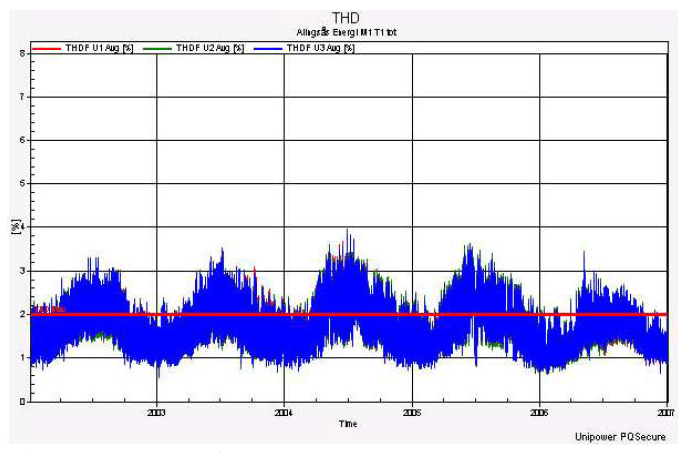
Modern power quality meters do not only measure THD and individual harmonics but also include additional harmonic parameters. The result is a complex set of adequate data that must be managed and handled in an effective and appropriate way if harmonic measurements are implemented in a larger scale. The trend of Harmonic measurements today is towards continuous monitoring with permanently installed meters. Long term monitoring of harmonics also provides effective means for planning. Example below shows 5 years of THD data. Seasonal fluctuations are present, but the long term trend is stable.
Fig.2. Seasonal fluctuation of THD in a MV station at distribution level.
POWER HARMONICS DIRECTION
Modern PQ Monitors do often also measure the Harmonic Phase Angle, i.e. the phase angle between each voltage and current harmonic. For a standard three phase installation that mean additional 150 parameters in addition to the 300 individual voltage and current harmonics recorded.
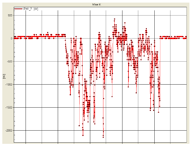
The harmonics phase angle is raw data from which the so called power harmonics can be derived. If using a PQ meter like the UP2210 or Unilyzer 902 the power harmonics can be shown with direction (+/-) thereby facilitating the interpretation of the harmonic flow, i.e. search for the harmonic source and at the same time reducing the data storage capacity.
Fig.3. Power harmonic flow.
Negative indicates the source is downstream the measure point.
3SEC MAX HARMONICS
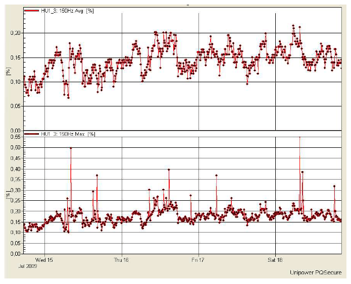
The harmonic limits in the standards are usually specified as the 10-min averages. There are however fluctuating harmonic loads today that are dangerous even though the duration is short. A new need for measuring the 3sec Maximum Harmonics has therefore arised. For such applications the PQ Meter continuously calculates 3sec harmonics, storing the Maximum value for each seleceted time period, normally 10-min, if IEC 61000-2-2, IEC 61000-2-12 or EN 510160 is being applied.
Fig.4. Example: 3sec Max values and 10-min averages for 3rd Harmonic Phase 1.
Today also the IEC 61000-3-6 specifies the need for measuring the 3sec Max Harmonics.
THE NEED FOR A HARMONIC INFORMATION MANAGEMENT SYSTEM
Harmonic measurements of today is no longer just THD measurements even though the number of THD parameters has increased (see below). As we have seen above up to approx 500 harmonic related parameters are to be calculated, stored and evaluated for each storage interval. In addition harmonic measurements are no longer just for troubleshooting purpose, but for contractual verification of the power supply and for preventive purposes.
Fig.5. Example of THD parameters derived from PQ analyzer Unilyzer 902 and UP2210.
The process of polling the data and making the in-depth data analysis is no longer efficient to make in a manual way when the number of measure points grow from just a few to hundreds and thousands of measure points in the transmission and distribution network. Neither is it a quality assured process. Instead a need for automatic handling of the harmonic data has arised. The characteristics of such a system are:
Automatic polling of harmonic data into a central database.
Data compression techniques for efficient transfer of data and data storage.
Automatic report generation scheduled on a weekly basis to provide summary statistics
Supervision of individual harmonic parameters with alarm functions
ON-LINE MONITORING OF INDIVIDUAL HARMONICS
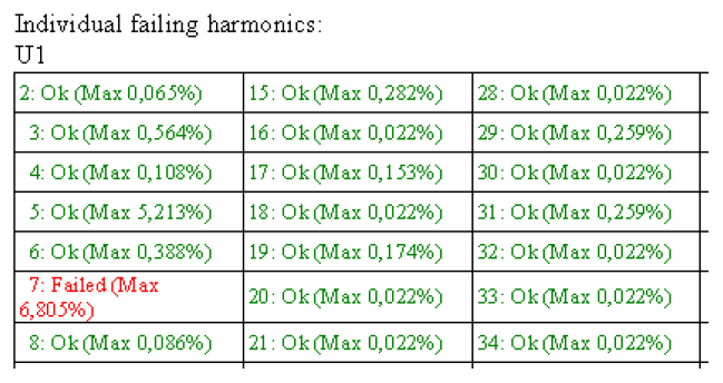
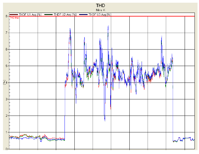
In a mining industry in northern Europe a Harmonic Information Management System, Unipower PQ Secure, was implemented and on a normal basis the harmonic levels were within control. In January 12th, 2008 the system manager however received an email from the Harmonic Information Management System notifying that in one measure point the 7th individual harmonics were outside specified control limits according to IEC 61000-2-12. Still however the THD was reported being inside control limits.
Fig.6. 7th Harmonic failing (see table of limits – Fig 1)
At site it could be concluded that one major filter had been disconnected by service personnel by mistake, and it could immediately be reconnected before any further damage and losses occurred.
Fig.7. THD value goes high when the filter is disconnected.
However the specified THD control limit is not violated. Without a Harmonic Information Management System in place monitoring the individual harmonics the filter would probably remained disconnected until the annual inspection or a possible failure occurred according to local management.
CONCLUSION
The international trend for Harmonic measurements is towards permanent supervision of harmonics in the transmission and distribution networks. The scale of implementation calls for an automated system for data gathering and automatic data analysis where both operators and authorities can receive scheduled weekly statistical information defining network status. Supervision and alarm functionality for all harmonic parameters also makes it possible to assure quality and keep harmonic levels in control in a preventive approach.
The challenge of tomorrow is not only to retrieve reliable and norm compliant harmonic data from the network, but also to manage this data in a reliable and cost effective way.
About Unipower: Unipower AB offers a wide range of products for Power Quality measurements and Smart Grid systems.
Originating from a Swedish ABB company in the mid 80’s, Unipower has developed a competitive edge within the field of Power Quality and Smart-Grid solutions. We focus on norm compliance equipment, with a special focus on the requirements for power generation, transmission and distribution.
Our product lines reach from traditional portable PQ analysers to fully integrated and automated Power Quality Management systems for continuous supervision of the energy supply.
• Its small size together with the IP65 protection and ruggedness makes Unilyzer 900 an ideal tool for all field measurements. It has no moving parts and has been tested in real, tough environments.
• The instrument complies with IEC 61000-4-30 Class A for Power Quality measurements, which guarantees highest reliability in every advice and conclusion.
• Its standard memory allows data to be stored for 3 months. In case of a power failure it has an internal battery backup keeping the instrument going.
• The UP-2210 unit works as an advanced power quality meter and at the same time as a fault recorder. All of the power quality parameters can be analyzed in accordance with voltage quality standards such as the EN 50160 or national regulations such as the Swedish EIFS. The UP-2210 unit captures both steady state disturbances (harmonics, flicker etc.) as well as rapid voltage changes (sag/swell events and fast transients). The nodes in the PQ Secure system consist of UP-2210 meters.
• Advanced 3-phase Power Quality and Transient Monitor
• The UP-2210 is a full-featured, norm-compliant power quality monitor capable of detecting any disturbances encountered in a network.
Published by 1. Edyta KUCHARSKA, 2. Katarzyna GROBLER-DĘBSKA, 3. Jerzy BARANOWSKI, 4. Waldemar BAUER, 5. Nataliia KASHPRUK, AGH UNIVERSITY OF SCIENCE AND TECHNOLOGY, KRAKOW, POLAND ORCID: 1. 0000-0001-6551-5062; 2. 0000-0003-3062-5987, 3. 0000-0003-3313-581X, 4. 0000-0002-8543-0995, 5. 0000-0001-5599-5509
Abstract. The article describes the use of ERP systems to support the management of companies in the energy industry. It points out the functional areas of these systems, which, apart from standard modules, are necessary for effective decision-making. Current challenges for the development of systems are presented, including methods of artificial intelligence, machine learning, data analysis and prediction, as well as new technological solutions.
Streszczenie. W artykule opisano zastosowanie systemów ERP do wspomagania zarządzania przedsiębiorstw z branży energetycznej. Wskazano obszary funkcjonalne tych systemów, które oprócz standardowych modułów są niezbędne do efektywnego podejmowania decyzji. Przedstawiono aktualne wyzwania dla rozwoju systemów, uwzgledniające metody sztucznej inteligencji, uczenia maszynowego, analizy i predykcji danych, a także nowe rozwiązania technologiczne. Systemy ERP w energetyce – możliwości i wyzwania
Keywords: ERP systems, data analysis, energy industry. Słowa kluczowe: Systemy klasy ERP, analiza danych, przemysł energetyczny
Introduction
ERP (Enterprise Resource Planning) is a category of business management software, typically a suite of integrated applications. ERP apps have been commonly used to manage many trades all over the world for many years, include the energy industry. In most countries, the energy industry is a strategic market sector often overseen by governmental bodies. Energy companies create intelligent enterprises based on intelligent cloud services that streamline and simplify operations [1]. Regardless of they and the enterprise type, power plant (coal, thermal, hydro, nuclear, solar) or electricity distributor, a reliable management approach is needed. In this sector, it is extremely important to implement the ERP system with specific, sectional functional and following the selected technological innovations. In this paper, we discuss the current requirements for ERP systems and emphasize the challenges in the development of IT systems in the energy industry in Poland.
Application of ERP systems
ERP systems integrate the organization’s business processes into the main functional areas and enable communication between all departments and divisions of a company. They include core software components, often called modules, with a common database. According to Gartner’s definition [2], ERP tools share a common process and data model, covering broad operational end-to-end processes.
The modular design of an ERP system incorporates distinct business modules which are independent of each other and could be deployed separately. Each module deals with different functions of a specific department of the organization. The individual ERP systems have their own structure, but we can distinguish the following areas as modules:
• Finance comprises tools for accounting and financial. It includes billing, payments and account reconciliation, which may be performed automatically. The module settings must be complied with the relevant regulations of the country. The module also prepares various reports in which we can check the profits and losses.
• Supply Chain Management includes all processes that transform raw materials into final products. It comprises many detailed elements in this area and procurement, storing, and delivery are the main.
• Inventory Management provides information about current stock and predicts future market demand. It may also include tools to manage storage space efficiently for optimum utilization.
• Manufacturing optimizes production capacity, production planning and product scheduling, helps in managing the inventory and quantities of manufactured products under the demand.
• CRM organizes all customer data, high-performing campaigns, and efficient service. Advanced functionalities of CRM provide you with data analytics and reports to gauge customer behavior, buying patterns, and satisfaction levels.
• Human Resources Management handles issues related to employees, such as hiring, training, development, payroll, safety, wellness, benefits, motivation, and administration.
• Business Intelligence includes tools for analyzing current and historical data to support more effective strategic, tactical, and operational insights and decision-making. Advanced functionalities provide data mining, data visualization, and data tools to help organizations make better data-driven decisions.
• Service Management supports the service company’s processes. It focuses on service teams, their time and productivity management, task, and route planning.
• Project Management provides skills, tools and techniques required to manage and account for projects. It supplies daily monitoring of expenses and work performed according to goals or budgets for each project.
ERP modules automate and support a range of administrative and operational business processes. They must operate in real time with regular updates of tasks’ status and fast execution of all requests.
According to the Panorama report for 2018 [3] enterprises that have implemented an ERP system with success have 80% higher information availability, 55% face better data reliability and 44% get improved productivity and lead time. But only 42% of respondents company in 2018 would deem their ERP Implementation a success. Thus, it is very important to choose the right ERP software. The type of activity of the enterprise and its specific requirements has a huge impact on the choice of system.
Requirements of ERP in energy industry
In the energy industry, requirements and tasks of IT systems supporting and managing the operation of power plants are specified in the National Energy System and include requirements imposed by the European Union. Because of the strategic nature of these enterprises, the aspect of IT security and the vulnerability of the system to the potential possibility of a cyber-attack are extremely important. Other system requirements will be for power plant and energy operators.
Fig.1. The basic structure of ERP
The main requirements for the power plant IT systems are determined of the available electrical power, organization of fuel supplies and their consumption, monitoring the operation of equipment, supporting the work of the power plant engineer, power plant operation control at the state level and support for research activities, financial processes, human resources, and administration. All power plants operating in Poland are part of the National Power System. Besides standard ERP system modules such as finance, HR, distribution, manufacturing, service and the supply chain in the energy industry, these systems should also support the following specific functionalities:
• Asset management, because power plant construction, maintenance of the power grid, analysis of the existing grid requires careful tracking and management. Handle the records of thousands of spare parts and consumables, as well as planning repairs, supplying spare parts, ordering, and accounting for repair and maintenance works.
• Geospatial planning is important for the energy sector to connect resources with geospatial data, such as plant locations or regional energy distribution.
• Then, for energy corporations, power outages are one of the biggest problems. The key challenges in this industry are avoiding downtime, extending a life cycle, and reducing repair costs. Failure management functionality addresses them. Because when the installation is down, the company receives no money and must also spend money on troubleshooting.
• Risk management warning of potential threats, e.g., related to natural disasters, so you can prepare contingency plans.
• Complicated project management used to manage the full life cycle of projects. The solution fully integrated with other system components from areas such as finance, supply, warehouse, sales orders, production, design, human resources, documentation management, and asset and service management, enabling full project management related to infrastructure development. The main requirements for the energy operators’ IT systems are:
• schedule for consumption readings, to optimize the work of the collectors and to predict the amount of the customer’s next bill early enough,
• To effectively manage customers, each of whom requires a separate billing, supply contract and different billing cycles. For example, issue a sales document every month invoices based on monthly consumption readings and billing according to actual consumption invoices based on a six-month calculation period. For the period between meter readings, it is necessary to generate budget billing plans. Thus, the following functionality is needed: consumption calculation, budget billing plans, calculation of electricity consumption for customers,
• The functionality of managing basic technical data, device installations and measurement results is required.
• Energy companies contact other companies, such as distributors or builders, as well as individual clients, such as end-users. Customer services should have multiple levels — from phone support to technical support — and associated costs and include services like issue fixes, incident resolution.
Table 1 shows list of specific requirements for power plant and energy operators’ companies.
Table 1. List of specific requirements for energy industry companies.
.
ERP systems in energy industry
According to the [4] in the worldwide energy industry, the most significant ERP software are SYSPRO, INFOR, SAP Business One, Sage X3 ERP, Microsoft Dynamics AX, S2K Enterprise, NetSuite ERP, IFS Applications 10, Cetec ERP, Priority Software ERP, E2 Manufacturing and Global Shop Solutions.
In Poland, in this sector, in huge companies, the most popular systems are SAP, IFS Applications and Microsoft Dynamics. The following chart (Fig.2.) presents a comparison of ERP systems in Polish used in energyproducing companies and energy operators.
IFS Applications 10
IFS offers ERP, EAM (Enterprise Asset Management) and FSM (Field Service Management) software for the energy, utilities and mining sectors [6]. The system uses many years of experience and extensive knowledge about the specificity of energy companies and about the problems they face. Solution IFS “Electricity Transmission and Distribution” provides functionalities for managing complex transmission network assets, optimizing asset performance management, meeting all budget and cost goals of the organization in terms of technical infrastructure maintenance. It allows to optimize service delivery processes which affect improving customer satisfaction.
Fig.2. ERP systems in Polish energy industry.
IFS offers project and asset management and service management functions with core ERP functions for the power transmission and distribution industry. It provides the functionality for customers who specialize in electricity transmission, power distribution networks, field services and the operation of smart meters.
IFS supports breakthrough technologies appear in the energy market and customer requirements are changing. IFS software supports the electricity generation market that is constantly changing, and the cost of renewable energy is getting lower.
IFS provides ERP and EAM solutions for both on premises and cloud-based applications.
SAP/SAP in energy data management has comprehensive solutions and provides all steps for profile-related data, from collection, validation, estimation, storage, and provisioning. It enables energy settlement or billing.
SAP supports requirements for various types of billing options, such as time of use, real time, or critical peak. It is possible to balance energy quantities, energy schedule management, and energy portfolio management in real time [7,8]. Two other modules, SAP Field Service Management and SAP Intelligent Asset Management, are very useful in energy companies’ activity SAP Field Service Management can help improve the efficiency and productivity of field service operations by linking and streamlining data to service processes, improve decision making, optimize route planning, and reduce costs. SAP Intelligent Asset Management facilitates collaborative resource management and allows you to take full advantage of the Internet of Things (IoT).
An interesting solution supporting current trends is SAP E-Mobility – a new, cloud-based solution for the operation of a large-scale electric vehicle charging infrastructure network. It enables the creation, operation, and management of charging infrastructure networks to transition to sustainable and comfortable electric mobility for individuals.
Microsoft Dynamics
Microsoft Dynamics provides tools for the energy market to design, manage, and install all kinds of solutions like oil, gas, biomass, water, solar, wind, and geothermal. It supplies an energy consumption, energy trading, compliance management, production, and distribution management.
System Microsoft Dynamics includes resource and project management functionalities, capabilities to analyze customer insights, tools for trend predictions, and sales and marketing automation.
It uses Cloud computing and AI to manage the logistics to provide households and companies with energy.
The solutions of the software producer also apply to renewable energy. It supports using the Internet of Things to generate, use and distribute energy from wind, water, the sun, or other sustainable sources effectively.
Challenges of ERP in energy industry
Here have been significant changes in recent years in the energy trade. Modern, efficient technology for generating, transmitting, and storing electricity causes that IT tools should propose new functionalities to manage energy more efficiently. The most important challenges of ERP in the energy industry are as follows.
Distributed generation – new and technologically advanced solar farms or wind farms are emerging. Small hydropower plants are also becoming popular. They are a relatively cheap source of energy and can quickly change the generated power depending on the demand. ERP systems should also include management of energy production, which merges the classic and alternative way.
Treating data as an assetis one of the research trends. Recently, data discovery offered great opportunities for supporting decision making and optimization of management activities. Data in ERP systems and converge different data sources for deeper intelligence [9]. In the energy industry, both predictive applications for demand and supply forecasting as well as predictive maintenance solutions are needed, e.g., to predict the amount of mandatory purchase of energy from micro-installations, predictive maintenance to predict machine failures and situations requiring action by using huge amounts of historical data and power computing.
Automation and robotization of business processes in ERP should effectively support enterprise and can cause improvements in overall employee experience and a reduction both in cycle time and in quality issues, and rework associated with manual data entry.
ERP system can be also extended through the Internet of Things to track inventory levels, predictive maintenance, reported location and shipment tracking [8].
Using wearable tech may be very important in enterprise management thanks to combining data analysis and prediction. This will not only allow employee and energy plant monitoring, but can significantly affect improving employee safety and field service.
The equivalent of augmented reality should be one technology necessary in future ERP. Augmented reality (AR) means viewing the objects/things on a computer with a feel of the real world. It may effectively reduce the complexity of maintenance and service operations. An example is a breakdown machine repair in a manufacturing unit when instead of calling and waiting for the specialist to arrive and repair it on-site, the repair can be done remotely using the actual physical real picture of the machine.
Conclusion
The article presents aspects of supporting the management of an energy enterprise by ERP systems. IFS Application and SAP have the most comprehensive solutions necessary in the energy industry and aims to be a leader in this area. However, the IFS system includes good asset management and machine service but does not have solutions related to current trends in automation and prediction. SAP proposes good customer management but hasn’t a specialized solution for power plants.
Published by Unipower AB, Metallgatan 4C, 44132 Alingsås, Sweden. Email: info@unipower.se
Introduction
This case study explores how advanced power quality measurement technology facilitated the diagnosis of severe power quality disturbances in a bus depot. These disturbances, which neither the bus operator nor the bus manufacturer initially attributed to electrical quality issues, were ultimately traced to deficiencies in the depot’s charging infrastructure.
Background
A bus depot, integrating both AC and DC charging infrastructure, was experiencing operational disruptions. The facility contained AC chargers (22 kW) designated for minibuses and DC fast chargers (200 kW) for larger electric buses. Depot operators observed that the AC chargers were intermittently failing when the DC chargers where in use. These issues impacted vehicle availability and overall operational efficiency. The root cause of these disruptions remained undetermined until an extensive power quality analysis was conducted.
Figure 1. Aerial view of the bus depot. Large buses are DC charged; minibuses are AC charged (overnight charging)
Diagnostic Assessment
A power quality investigation revealed that the power disturbances originated from the absence of necessary electrical filters in the DC chargers. Without these filters, the operation of DC chargers induced significant harmonic distortions in the local voltage, interfering with the stability of the AC charging units.
Power Quality Analysis
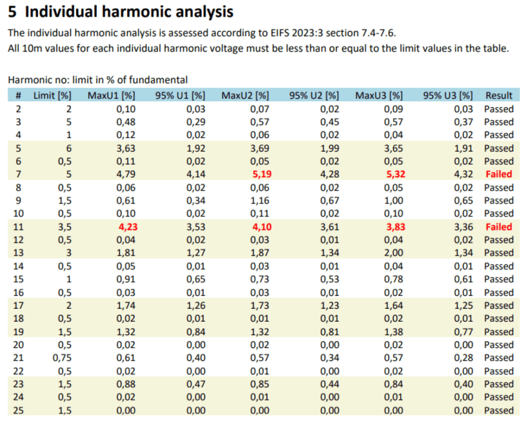
The measurement data indicated that the Swedish power quality standard (EIFS) had been exceeded due to harmonic content in the 7th and 11th harmonic. EIFS is a local adaption of the European EN50160 norm.
Figure 2. 7th and 11th Harmonic are failing
Additionally, the analysis revealed that the power factor was significantly below optimal levels, causing energy inefficiencies within the depot’s electrical distribution system.
Implementation of Mitigation Measures
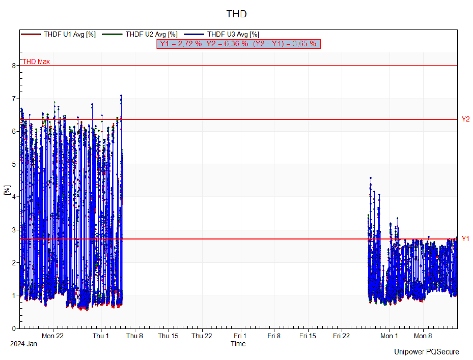
Following the identification of these power quality issues, the DC charger manufacturer installed appropriate electrical filtering solutions. A subsequent measurement campaign was conducted to assess the effectiveness of these interventions. The results demonstrated a significant improvement:
• Substantial reduction in harmonic distortions, bringing them within regulatory compliance limits.
Figure 3. THD before and after filters were installed
• Power factor improvement from 88% to 97%, enhancing overall energy efficiency by 9%.
Figure 4. Power factor before and after filters were installed
Lessons Learned & Next Steps
• Implement continuous monitoring: Regularly measure power factor, harmonic distortion, and other vital parameters to detect potential issues before they escalate.
• Evaluate expansion opportunities: As the electric fleet grows, continuously assess whether the existing filters, chargers, and electrical network remain adequate.
• Strengthen collaboration with manufacturers: Ongoing dialogue with both bus and charger suppliers helps ensure that proper filters and components are in place from the outset.
• Analyze economic implications: Beyond energy savings, conduct a return-on-investment (ROI) analysis of the filter installation and the improvements in system stability.
• Educate relevant staff: Ensure that electrical technicians and depot managers understand fundamental power quality principles, enabling rapid response to emerging anomalies.
This case study underscores the critical role of advanced power quality diagnostics in identifying and resolving electrical disturbances. By systematically analyzing power parameters and implementing targeted mitigation strategies, significant improvements in charging infrastructure reliability and energy efficiency were realized. The findings highlight the necessity of continuous power quality assessments for ensuring optimal performance and compliance in electric bus depots.
About Unipower: Unipower AB offers a wide range of products for Power Quality measurements and Smart Grid systems.
Originating from a Swedish ABB company in the mid 80’s, Unipower has developed a competitive edge within the field of Power Quality and Smart-Grid solutions. We focus on norm compliance equipment, with a special focus on the requirements for power generation, transmission and distribution.
Our product lines reach from traditional portable PQ analysers to fully integrated and automated Power Quality Management systems for continuous supervision of the energy supply.
The main problem with transients in the electrical network is that a high voltage potential might break the isolation barrier in for example cables or other equipment in the electrical network. It may also harm semiconductors that are sensitive of high voltage.
A transient voltage is by definition short in time and typically consists of frequencies higher than 500Hz. Typically sources of transients are switching in the network and lightning. A capacitor switching usually consists of frequencies below 1kHz. Fast transients like lightning that occur in the electrical network become flattened because of dispersion in the grid.
The Transient Test Pulse
The typical transient test pulse that is used in testing equipment like cable joints and breakers are designed in a way that should correspond to the profile of a real lightning strike. The rise time for this pulse is 1.2us and the fall time is 50us.
Capturing Transients
With a transient of the lightning type the chance of missing the damaging top voltage is high if the sampling rate of the instrument is not high enough. A common practice is to use a sampling rate of 10 times the speed of the event that is recorded. In the case of catching a high frequency switching in the network or a lightning the sampling rate should be about 10Mhz in order not to miss the top voltage level.
Peak detectors versus High Speed Sampling
The disturbance in the picture below is sampled with a sampling speed of 1 MHz. The dots correspond to the sample points. The high amplitude is not captured in this case because no sampling is done at the highest point. The peak detector does not have this limitation; they will follow the signal to the highest point and store that value.
A sampling speed of 1 MHz
UP2210 and Unilyzer 902 Transient Detection
The power quality analyzers UP-2210 and Unilyzer 902 are equipped with transient analysis that is enhanced with peak detectors. A transient recorder usually samples the signal at discrete points. This means that you will know the actual input level only in the sample point. In order not to miss any information you will need to increase the sampling speed. Even with very high sampling speed the equipment will be ‘blind’ between sample points. With a high sampling speed the memory is rapidly consumed and in order to save memory only a fraction of the disturbance could be stored.
With the use of peak detectors we can solve all of this problems. The peak detector follows the signal all the time without missing any signal deviation. When the peak detector activates it will trap the highest (or lowest) value that occurred between the sampling points. This allows us to save memory without loosing any information of interest. Any transient with high potential that might harm the isolation will be registered.
The UP-2210 and Unilyzer 902 has both positive and negative hardware peak detectors. The peak detectors have a response time less than 1us.
The example below is produced with an arbitrary generator that creates one transient point in the most positive part of the period and one transient is made in the most negative part of the period. The duration of each transient in this example is 1.2 us. All important transients is detected without high sampling rate.
Fast transients (1.2 us) captured with Unilyzer 902
About Unipower: Unipower AB offers a wide range of products for Power Quality measurements and Smart Grid systems.
Originating from a Swedish ABB company in the mid 80’s, Unipower has developed a competitive edge within the field of Power Quality and Smart-Grid solutions. We focus on norm compliance equipment, with a special focus on the requirements for power generation, transmission and distribution.
Our product lines reach from traditional portable PQ analysers to fully integrated and automated Power Quality Management systems for continuous supervision of the energy supply.
• Its small size together with the IP65 protection and ruggedness makes Unilyzer 900 an ideal tool for all field measurements. It has no moving parts and has been tested in real, tough environments.
• The instrument complies with IEC 61000-4-30 Class A for Power Quality measurements, which guarantees highest reliability in every advice and conclusion.
• Its standard memory allows data to be stored for 3 months. In case of a power failure it has an internal battery backup keeping the instrument going.
• The UP-2210 unit works as an advanced power quality meter and at the same time as a fault recorder. All of the power quality parameters can be analyzed in accordance with voltage quality standards such as the EN 50160 or national regulations such as the Swedish EIFS. The UP-2210 unit captures both steady state disturbances (harmonics, flicker etc.) as well as rapid voltage changes (sag/swell events and fast transients). The nodes in the PQ Secure system consist of UP-2210 meters.
• Advanced 3-phase Power Quality and Transient Monitor
• The UP-2210 is a full-featured, norm-compliant power quality monitor capable of detecting any disturbances encountered in a network.
Publishd by Ahmed A. Abdullah AL-KARAKCHI1, Enaam ALBANNA2, Alya H. AL-RIFAIE3, Northern Technical University (1,2,3) ORCID: 1. 0000-0003-1151-3015; 2. 0000-0002-3974-0116; 3. 0000-0002-7978-2193
Abstract. Unbalanced network voltage damages utility and end-user equipment. Electrified trains, single-phase distributed generators, and line-toline connected industrial loads can increase voltage imbalances. Using Dynamic Voltage Restorer (DVR) at appropriate places is one way to reduce imbalance in practical networks. This research proposes a new technique for managing DVR to improve voltage profile. The simulation results imply that real-time implementation of the suggested controller is practical and resilient.
Streszczenie. Niezrównoważone napięcie sieciowe uszkadza sprzęt komunalny i użytkownika końcowego. Zelektryfikowane pociągi, jednofazowe rozproszone generatory i obciążenia przemysłowe połączone między liniami mogą zwiększać nierównowagę napięcia. Używanie dynamicznego przywracania napięcia (DVR) w odpowiednich miejscach jest jednym ze sposobów zmniejszenia asymetrii w praktycznych sieciach. Badanie to proponuje nową technikę zarządzania DVR w celu poprawy profilu napięcia. Wyniki symulacji sugerują, że implementacja sugerowanego kontrolera w czasie rzeczywistym jest praktyczna i odporna. (Dynamiczny przywracacz napięcia do ograniczania asymetrii napięcia i poprawy profilu napięcia w sieci dystrybucyjnej)
Keywords: DVR, Voltage unbalance, voltage profile, p-q Theory, Fuzzy Logic. Słowa kluczowe: nierównowaga napięć, dynamiczne przywracanie napięciea.
Introduction
The electric power system is a network that transmits, supplies, and distributes electricity using electrical components. The three major components of power systems are generation, transmission, and distribution, which provide power to nearby residential complexes and large industries [1]. The network consists of three phases, which are three current and voltage signals (peak value) of equal magnitude but shifted by 120o as a phase difference between phases. If either the magnitude or the phase shift, or both, do not meet the standard, this is referred to as unbalance condition. In the majority of cases, the world’s modern power system uses AC three-phase power in a typical large-scale configuration for power transmission and distribution [2][3]. Single-phase loading is the leading cause of voltage unbalance. Line voltage unbalance caused by asymmetry of either current or voltage or both asymmetry of current and voltage at the same time [3]. Voltage unbalance is the most commonly occurring problem in power quality cases today, particularly in low voltage distribution systems. Voltage unbalance is the maximum amplitude phase voltage deviation from the average nominal phasemagnitude voltage [4]. In a similar way, voltage unbalance—which is also regarded as power quality—is described in [5] as the ratio of the difference between the greatest and smallest amplitudes of phase voltage magnitude to the mean phase-magnitude voltage. The power quality delivered to end users can be estimated as a constant magnitude of voltage, which means balanced in phases, zero voltage deviation, around unity power factor, fixed frequency, no variation in voltage like sags swells conditions, no any interruptions in power supply and also the ability to protect and isolate faults very quickly. The application of a new design controller in a distribution system to provide high reliability of an electrical power system to end users, which has increased the industry’s standing in the deregulated power network around the world. The following are the primary causes of voltage unbalance [6]: 1. The parameters of both the distribution and transmission lines, as well as the generators, are unsymmetrical [7]. Unbalanced voltages will result if the consumer load on one or two phases differs from the load on three phases. 2. An unbalanced current that passes through the system impedance causes an unbalanced voltage drop. 3. Transformer banks in open delta connection. 4. The faults in power transformer. 5. The power supply unsymmetrical impedance conductors. On the load side, the effect of voltage unbalance in equipment can be explained as follows [8]:
1. Voltage unbalance in rotating machines causes a reverse magnetic field, which causes torque to decrease due to heating of machine windings [9].
2. Damaging the power supply’s wiring (generators and transformers).
3. Unbalanced voltages at the terminals of a motor result in an unbalanced phase current of 6 to 10 times the motor’s full load.
4. It also reduces motor torque capability.
For many years, numerous techniques, including series capacitors, shunt reactors, boosting transformers, and, most recently, the VAR compensator “reactive power compensation,” have been utilized in the industrial sector for compensating voltage unbalance in electric distribution systems. Many researchers have proposed various mitigation techniques for correcting variation in line voltage and improving the voltage profile in the distribution network; This involves adjusting the medium feeder voltage, rearranging the phases, and balancing the phases between the distribution energy converter banks and the radial layout of the distribution system [5]-[10].
The previously mentioned techniques primarily target the medium and low voltage sides of the distribution network. However, Consumers and the power company were hoping for more efficient solutions to problems of voltage variation and voltage profile improvement, but the proposed ones were actually less effective.
Dynamic Voltage Restorer
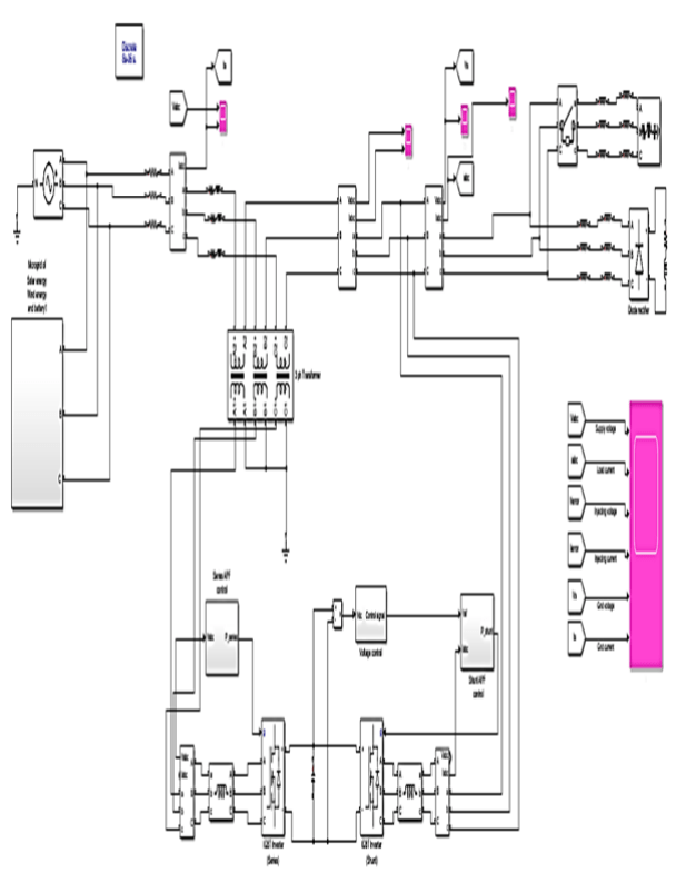
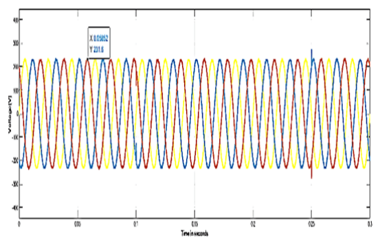
The DVR provides three-phase controllable voltage in amplitude and phase shift (vector), which adds to the line voltage to restore the voltage in the load side to pre-disturbance levels, as illustrated in Figure (1) [11].
DVR is comprised of signal control, measuring parameters, and a power unit. Figure (2) [12] depicts the main components:
Fig.1. Schematic diagram of DVR System.Fig.1. Schematic diagram of DVR System
Fig.2. Elementary system with an DVR
The following are the three types of DVR control strategies [13]:
• In-phase • Pre-Sag • Minimum Energy
All of these strategies for compensating line voltage are depicted in Figure 3 [14].
Fig.3. Control DVR voltage (a) Pre-Sag control (b) In-Phase control (c) Minimum Energy control
The DVR injects the line voltage by adding a voltage with an adjustable amplitude and phase shift in series with it., regardless of its magnitude and phase angle. As a result, the voltage after DVR will be the sum of the line voltage and the DVR voltage VDVR, as shown below:
.
The DVR voltage can increase or decrease magnitude and phase voltage by reversing the voltage polarity of VDVR (180° phase-shifted). Depending on the above strategies, the DVR voltage can add amplitude only, amplitude and phase shift, or voltage amplitude and phase shift depends on minimum energy. The second type of strategy used in this proposed design was in-phase compensation, in which the controller checks the amplitude and phase angle of the line voltage to inject the compensated voltage. It is also worth noting that the DVR has a quick response time of less than a cycle, allowing it to track the line voltage and compensate in abnormal conditions [15].
Measuring the Line Voltage
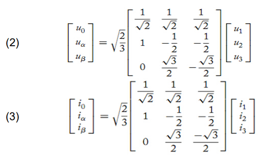
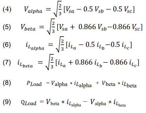
Instantaneous power theory, also known as p-q theory, was used for quick response when measuring line voltage. Akagi et al. developed this theory in 1983 with the goal of applying it for measuring and controlling active and reactive power for power flow control or filtering. P-q theory is based on Time Domain, and it can be applied in both steady-state and transient-state conditions. It can also be applied directly to instantaneous voltage and current waveforms in power systems, allowing for real-time control of all power parameters such as voltage, current, active power, and reactive power. This theory’s main advantage is its simplicity and clarity in calculations, which require only algebraic calculations with the exception of separating alternated and mean power values. The p-q theory is implemented using the Clarke Transformation for a stationary reference, which eliminates the need for an angle ad in d-q or abc transformations. This transformation is performed from a-b-c coordinates to α-β-0 coordinates and vice versa [16].The DVR voltage can increase or decrease magnitude and phase voltage by reversing the voltage polarity of VDVR (180° phase-shifted). Depending on the above strategies, the DVR voltage can add amplitude only, amplitude and phase shift, or voltage amplitude and phase shift depends on minimum energy. The second type of strategy used in this proposed design was in-phase compensation, in which the controller checks the amplitude and phase angle of the line voltage to inject the compensated voltage. It is also worth noting that the DVR has a quick response time of less than a cycle, allowing it to track the line voltage and compensate in abnormal conditions [15]. Measuring the Line Voltage Instantaneous power theory, also known as p-q theory, was used for quick response when measuring line voltage. Akagi et al. developed this theory in 1983 with the goal of applying it for measuring and controlling active and reactive power for power flow control or filtering. P-q theory is based on Time Domain, and it can be applied in both steady-state and transient-state conditions. It can also be applied directly to instantaneous voltage and current waveforms in power systems, allowing for real-time control of all power parameters such as voltage, current, active power, and reactive power. This theory’s main advantage is its simplicity and clarity in calculations, which require only algebraic calculations with the exception of separating alternated and mean power values. The p-q theory is implemented using the Clarke Transformation for a stationary reference, which eliminates the need for an angle ad in d-q or abc transformations. This transformation is performed from a-b-c coordinates to α-β-0 coordinates and vice versa [16].
.
The two parameters p (active power) and q (reactive power) are then calculated as follows:
.
Where iα and iβ are orthogonal current, and vα and vβ are orthogonal voltage. The voltage after compensation is as follows:
.
To get phase voltage:
.
Voltage unbalance is calculated using the Maximum Deviation Method (MDM), and the voltage unbalance carried on by an unbalanced main load [17] is given: Voltage unbalance%= (MAX Deviation from V) ̸ Ṽ
.
Where v1, v2 and v3 are the phase voltage readings.
DVR Control Design
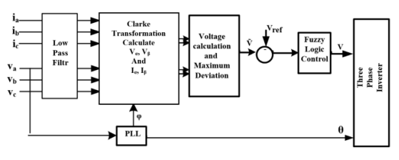
Figure 4 depicts the DVR control system’s block diagram structure. Line voltages and currents are measured from the line, and a filter stage was added to eliminate noise and harmonics. Clarke transformation is used to calculate the orthogonal two voltages and currents components (vα, vβ) and (iα, iβ). Equation 6 is used to calculate the compensated voltage, and the voltage unbalance is calculated using the Maximum Deviation method MDM; this voltage signal serves as feedback for the closed loop control system Fuzzy logic, where V∑ is compared to the reference voltage Vref set point of the line voltage to be compensated, and an error signal, verror, is generated.
Fig.4. DVR control system Block diagram
Fuzzy Logic Control System
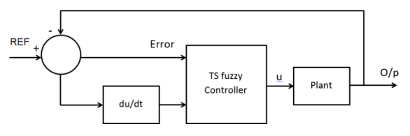
The Fuzzy logic control was used, which is adequate for approximate reasoning, especially in systems with mathematical model equations that are difficult to derive [18]. In this proposed study, Takagi-Sugeno TS inference mechanism systems are used. This study tunes Takagi-Sugeno ANN membership functions. Figure 5 depicts the Fuzzy logic control design. Fuzzy logic controller with adaptive learning capabilities using ANN, this approach can be easily trained, and the rule base of Fuzzy controller is reduced [19].
Fig.5. TS fuzzy control scheme
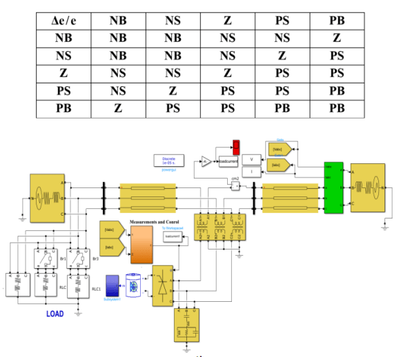
The Fuzzy control system is composed of five layers, each of which has parameters that do not require tuning (constants) or have parameters that do require tuning (variables) during the training stage. The input discourse universe is divided into five triangle form membership functions with 50% overlap, for two input signals error and Δerror, the control rule is 25 to result of linear functions as required to be set, as shown in Table 1. Figure 6 depicts the structure of the Fuzzy logic control design. Two groups of data are generated to tune the rules using adaptive fuzzy. There are two input vectors: Verror and ΔVerror, and the output is the modulation index “m.”
Simulation Study
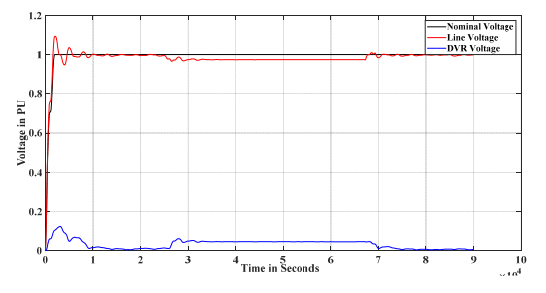
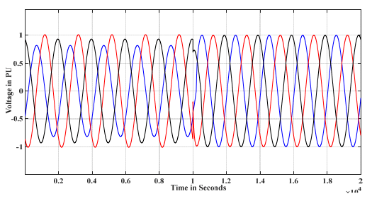
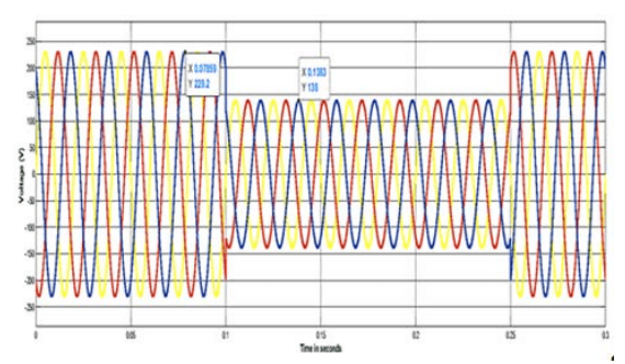
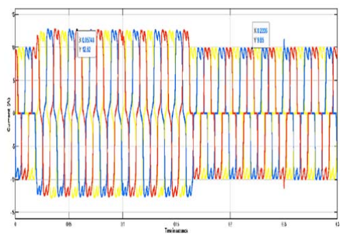
The proposed model is consisting of a low voltage feeder with a variable load and three branches for balance and unbalance load conditions. As shown in Figure 7, the DVR is connected to the load side to compensate for the load voltage. The simulation test begins by varying the three phase load, first in balance condition and measuring the line voltage, then at t=2.5 additional load add the voltage decrease as shown in Figure 8a, and compensation is done by injecting VDVR for balance load to compensate the voltage at sag condition as shown in Figure 8b. The drop in line voltage increased proportionally to the increase in load, with the maximum drop being 0.8 pu between 2.5 and 6.75 sec. Figure 9 depicts the injected voltage at the previously mentioned time interval. Figure 10 depicts the line voltage versus the DVR voltage under sag conditions. Figure 11 shows the action of the DVR at t=1 seconds and Figure 12 shows the injected compensated voltage in unbalance condition, respectively, to validate the DVR under unbalance voltage, a sudden heavy unbalance load changed. According to the results of Figures 11 and 12, the DVR has the ability to respond quickly to an unbalance condition and restore the line voltage to its nominal value.
Fig.6. Structure Fuzzy logic design
Fig.7. Proposed model for simulation
Fig.8. The waveforms of line voltage (a) before compensation (b) After compensation
Fig.9. The output of DVR
Fig.10. Line voltage with compensation
Fig.11. Line voltage at unbalance condition
Conclusions
In this proposed study, a DVR-based fuzzy logic controller has been installed on the load bus, and Simulations of voltage unbalance and sag condition have been used to investigate a number of abnormal conditions. The simulation results show that the action of a DVR with an adaptive controller improves the voltage profile in the distribution system and restores the voltage unbalance condition. The simulation was compared with and without compensation, as well as balance and unbalance conditions, with the balance condition for sag and the unbalance load for voltage unbalance. The DVR was able to restore the load voltage to its nominal value (within about 97%) in two conditions. The computation action time was approximately 10 msec; this response time is critical for tracking any change in real time. The simulation results in both conditions show that the Fuzzy Logic controller provides good response for the operation of the DVR.
REFERENCES
[1] Alya H. AL-RIFAIE, Sanabel M. ALHAJ ZBER, Noha Abed-ALBary AL-JAWADY, Ahmed A. Abdullah AL – KARAKCHI, “Analysis of faults on high voltage direct current HVDC transmissions system”, Przegląd Elektrotechniczny, issue. 2 pp. 49-53, FEB 2022. [2] ZBER, Sanabel Muhson ALHAJ, et al. “Simulation and Analysis of a VSC-HVDC Transmission System Based on DC Line-Line Fault.”, Przegląd Elektrotechniczny, issue. 8 pp. 69-72, AUG 2022. [3] T. D. Kahingala, S. Perera, U. Jayatunga, and A. P. Agalgaonkar,“Estimation of voltage unbalance attenuation caused by three-phase induction motors: An extension to distribution system state estimation,” IEEE Transactions on Power Delivery, 2019. [4] PKapil, C. Vibhakar, S. Rajani and K. Bhayani,” Voltage Sag/Swell Compensation Using Dynamic Voltage Restorer (DVR)”, International Journal of Application or Innovation in Engineering & Management (IJAIEM), vol 4, no 3, pp 1-8, 2013. [5] I. Afandi, P. Ciufo, A. Agalgaonkar, and S. Perera, “A combined mv and lv network voltage regulation strategy for the reduction of voltage unbalance,” in 2016 17th International Conference on Harmonics and Quality of Power (ICHQP), Oct 2016, pp. 318–323. [6] A. Damor and V. Babaria, ” Voltage Sag Control Using DVR”, National Conference on Recent Trends in Engineering & Technology India, pp 1-4, 13-14 May 2011S. [7] D. M. Soomro and et al “Mitigation of Voltage Sag Caused by Unbalanced Load by Using DFT Controlled DVR,” 2019 IEEE International Conference on Innovative Research and Development, 2019, pp. 1-6, 2019. [8] M. Sharanya, B. Basavaraja and M. Sasikala,” Dynamic Voltage Restorer (DVR) for Voltage Sag Mitigation”, International Journal on Electrical Engineering and Informatics, vol 3, no 1, pp1-11, 2011. [9] Pradhan, M., and Mishra, M. K.. Dual P-Q Theory based Energy Optimized Dynamic Voltage Restorer for Power Quality Improvement in Distribution System. IEEE Transactions on Industrial Electronics, 1–1., 2018. [10] Mohammed Y. Suliman and Mahmood T. Al-Khayyat, . “Power flow control in parallel transmission lines based on UPFC.” Bulletin of Electrical Engineering and Informatics 9.5 (2020), pp.1755-1765. [11] T. D. Kahingala, S. Perera, U. Jayatunga, and A. P. Agalgaonkar, “Estimation of voltage unbalance attenuation caused by three-phase induction motors: An extension to distribution system state estimation ” IEEE Transactions on Power Delivery, 2019. [12] S. Panda, and N. P. Padh,. “Comparison of particle swarm optimization and genetic algorithm for FACTS-based controller design”, Appl. Soft Compute., vol.8, no.4, pp. 1418-1427, 2008. [13] Harshita B., Kajol S., Navneet K. Effect of Voltage Sag and Voltage Unbalance on Induction Motor Drives. International Journal Of Advance Research, Ideas And Innovations In Technology (IJARIIT). 2017. 3(6). 258-263. [14] Harshita B., Kajol S., Navneet K. Effect of Voltage Sag and Voltage Unbalance on Induction Motor Drives. International Journal Of Advance Research, Ideas And Innovations In Technology (IJARIIT). 2017. 3(6). 258-263. [15] Anulal A. M, Archana Mohan and Lathika B. S, “Reactive power compensation of wind-diesel hybrid ystem using STATCOM with Fuzzy tuned and ANFIS tuned PID controllers”, International Conference on Control Communication & Computing India (ICCC), IEEE Conference,19-21 Nov,2015, pp. 325–330, 2015. [16] Alkhayyat, M.T., Suliman, M.Y., Aiwa, F.F. ,” PQ & DQ based shunt active power filter with PWM & hysteresis techniques”, Przeglad Elektrotechnicznythis, 2021 (9), pp. 78-84, 2021, doi:10.15199/48.2021.09.17. [17] G. Gupta and W. Fritz, “Voltage unbalance for power systems and mitigation techniques a survey,” IEEE 1st International Conference on Power Electronics, Intelligent Control and Energy Systems (ICPEICES), pp. 1-4, 2016, doi: 10.1109/ICPEICES.2016.7853717. [18] Mohammed Y. Suliman, ” Voltage profile enhancement in distribution network using static synchronous compensator STATCOM “, International Journal of Electrical and Computer Engineering (IJECE), Vol. 10, No. 4, 2020, pp. 3367~3374. [19] Alkhayyat, M.T., Suliman, M.Y., Aiwa, F.F., ” PQ & DQ based shunt active power filter with PWM & hysteresis techniques | Bocznikowy aktywny filtr mocy oparty na PQ i DQ z technikami PWM i histerezy “, Przeglad Elektrotechnicznythis, 2021(9), pp. 78–84, 2021.
Authors: Dr. Ahmed A. Abdullah Al-Karakchi , E-mail: ahmedalkarakchi@ntu.edu.iq; Enaam ALBANNA, E-mail: enaam.albanna@ntu.edu.iq; Alya Hamid Al-Rifaie, E-mail: alya.hamid@ntu.edu.iq
Source & Publisher Item Identifier: PRZEGLĄD ELEKTROTECHNICZNY, ISSN 0033-2097, R. 99 NR 6/2023. doi:10.15199/48.2023.06.38
Published by Ali HAMOODI, Rasha MOHAMMED, Bashar SALIH, Northern Technical University, Engineering technical college
Abstract. The objective of this work was to protect the transmission line (T.L.) from the lightning effect. In the last decades, several methodologies have been employed for the rise of lightning performance on the T.L Lightning with high values of current is a major cause of faults. Many types of current sources (AC, DC and pulse) were simulated to represent the current of lightning and the effect of each type on a metal-oxide arrester (MOV1, MOV2) and the load. The waveform of voltages and current at the (MOV1, MOV2) and the load have been drawn. It has been concluded from the comparison among the different cases that were made.
Streszczenie. Celem tej pracy było zabezpieczenie linii przesyłowej (TL) przed wyładowaniami atmosferycznymi. W ostatnich dziesięcioleciach zastosowano kilka metodologii w celu zwiększenia wydajności wyładowań atmosferycznych w T.L. Błyskawice z wysokimi wartościami prądu są główną przyczyną usterek. Symulowano wiele rodzajów źródeł prądu (AC, DC i impulsowe), aby przedstawić prąd wyładowania atmosferycznego i wpływ każdego typu na ogranicznik z tlenku metalu (MOV1, MOV2) i obciążenie. Narysowano przebiegi napięć i prądów na (MOV1, MOV2) oraz obciążeniu. Wywnioskowano z porównania różnych spraw, które zostały przeprowadzone. (Ochrona odgromowa linii przesyłowej wysokiego napięcia za pomocą ogranicznika przepięć)
Keywords: lightning, transmission lines protection, arrestors types, metal-oxide modelling. Słowa kluczowe: linia transmisyjna wysokiego napięcia, zabezpieczenia, ochrona odgromowa
Introduction
A lightning surge is a short-term irregular overcurrent created by lightning and momentarily applied to T.L. Lightning causes a quick shift in the electromagnetic field around T. L, resulting in an induced lightning surge. High current values are caused by lightning in the power structure, and several strategies and approaches are utilized to mitigate these challenges. Overvoltage is often of two types: fulgurite and changing [1].
The lightning strikes major electrical circuits connecting to both sides of the T.L structure, causing delays in lines and plans connected to T.L. As a result, it is critical to investigate a lightning strike for a reliable process of a control project; the discharge flow overvoltage is the key issue for the power structure and substation protection project. When lightning strikes the highest point of a transmission tower, a lightning current flows down to the lowest point of the tower and grounds; the voltage on the opposite side of the tower rises, causing a back flashover across an arc horn. Because of the considerable average return variation associated with lightning transients, a proper electrical type is necessary, and modeling investigations necessitate the whole creation of the lightning wonders and system elements. When it comes to eradicating the T.L and making preparations, lightning does the greatest damage. In electrical power networks, utilizing a surge arrestor to reduce or eliminate lightning flashovers or switching surges on distribution and transmission lines is crucial for overvoltage protection. A protection tube was an old type of surge arrestor. With the advent of the metal oxide arrester, with its superior energy capability, and with the adjustment of the quantity of earth covers, the utilization of arresters for the stronghold of lines has anticipated new energy and esteem. As a result, the flood arrestor is now in a dangerous situation where extraordinary current significance shots can keep the arrestor [2].
Effect of lightning on T.L.
When lightning strikes, it depends on a few factors: the level of the lightning represents the zone traversed by the line, the actual sizes, the general level of the line, and the presence of normally safeguarding objects, for example, structures and tall trees close to the line or different lines in a similar channel.
The total amount of lightning activity is represented by the number of lightning strikes per square mile on Earth each year. The actual line resorts to being a section that is pulled by the lightning gatherer and prompts drawing in streaks that would go after the ground distinctively over an area multiple times the width of the typical level of the above channel or protection wire .
This rationalization is typically known as an ingenious overview of a streak, understanding the width and shadow of the strains and the depth of lightning for an area, the calculation of a part of the road, the quantity, and the anticipated wide variety of moves as a result of lightning to the road in step with a mile in a year. The account wide variety will represent the everyday distribution of the statistical data, those numbers range from year to year with time and location because of the distinction within the top of the terrain and different signs and symptoms which include proximity to homes that defend the road from lightning strikes. [3].
Materials and methods
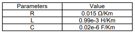
The real data of this work were taken from electric power transmission and distribution reference [4], These parameters are listed in the table (1).
Table.1 T.L parameters
.
The protection method used for T.L specifications, surge arresters is widely used to protect the T.L. metal oxide arrester and provide the best protection for T.L. The following components make up the fault simulation model are given as:
A metal oxide lightning arrester limits the overvoltage by means of disconnecting the road or by means of shifting to a voltage lower than the flash voltage to disconnect the road [5]. Flow dividers (surge arresters) are related on T. L with inside the center of the section and floor to sell the lightning act and to lower the fail level. Numerous special styles of arresters are accessible (e.g. with gapped or non-gapped metal-oxide) and all do in a like way, the motive is to the excessive impedance at typical operating voltages and develops low impedances via surge situations. Despite a large number of lightning arresters, they are still used with silicon carbide resistor arresters which are fixed today [6]. The simulation results show that the temporary raise in current at MOV1and MOV2 which is done by the lightning at 10kA lightning current is utilized as given in Figs.9 and10. On the other hand, a momentary rise in voltage in each arrester. After 0.03sec the arrester’s behaviour was steady state situation. the load current decreased during that time, and the load voltage increased where the lightning happens.
There are many types of lightning arresters, the two types used are metal oxide and suspension lightning arresters as shown in Fig.1 respectively. In this work, metal oxide types were adopted in the simulation.
The metal oxide device pillar, composed of the accompanying backing structure, includes the real active portion of the arrester. The pillar contains single metal -oxide resistors piled on top of apiece other, their distance conclusively defines the energy preoccupation and the current ringing ability. It is within the scope of periphery 30mm when used in the distribution system, insomuch 100mm or further for high-voltage and extra-high voltage discipline. The resistor of Metal oxide after is high between 20mm and 45mm.
Components
Metal oxide arrester consists of a saddle clamp, flex Joint, shunt, arrester body, disconnect and ground lead.
Working principle
The passing currents above the arrester in the part of the area may be useful. The voltage is very small for the power frequency so; the arrester practically makes it like an insulator. But, flow currents in the KA domain are inserted into the arrester, like in the event when lightning or swapping over-voltages happen, at that time the resultant voltage through its stations will continue low sufficient to keep the insulation of the connected appliance from the things of overvoltage. At a similar time, the escaping current runs over the arresters, this contains a big capacitive and a significantly lesser resistive section.
The function of this type of arrester is to process the system to hold off its voltage, limit the pass in voltage to a safe level with the lowest delay and filter and get the system back to its ordinary process type as soon as the passing voltage is blocked [2].
Lightning stroke machinery
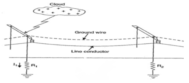
When charges accumulate in clouds, the lightning process occurs, as the charges are discharged into neighbouring clouds or to the ground. Basically, the process of the occurrence of lightning is an electric discharge of charges in the form of flashes from clouds with positive and negative charges. Charges in the cloud as given in Fig.2 pass when the lesser Part of the cloud is negatively charged at a temperature of -5°C although the positive charge is located at the top of the cloud at a temperature below -200C.
Fig.2. Lightning phenomena
Below the cloud, it is possible to form positive charges on the ground. In most thunderclouds, there is an area with limited positive grime located near the bottom of the cloud a 0°C. Charges formed in the kilo-coulomb range reaching a distance of about 50Km will be formed when lightning occurs, but the average current discharged by lightning is within limits KA [7]. The effect of lightning is the effect of a dense current of high strength and it increases first in the atmosphere, then in the solid state, or less at (the earth) [8- 10].
Lightning parameters
Lightning arrester is considered as the primary source for designing lightning protection devices to reduce over voltage on a transmission line. These parameters are given as:
• Peak current value of both first and subsequent • Stroke current wave shape
The size of the stroke charge and the magnitude of the return strike are key qualities to study the ultimate lightning force on the head of the T.L system.
There are two types of lightning strokes:
• Direct lightning strokes
Direct lightning stroke finishing on the T.L may affect in the happening that intrudes the power method, such as the above voltage. The lightning overvoltage is observed as the main reason for line isolation flashover, which can be separated into three types specifically back flashover, protecting failure and persuaded overvoltage [11-12].
• Indirect lightning strokes
Encouraged overvoltage happens when a clouds-to-earth lightning flashes crops a passing electromagnetic field, so makes important surge voltage on overhead lines in the area. The lightning-persuade overvoltage is in charge of the common errors occurring in circulation overhead lines. Though, these made voltages have an unimportant result on high-voltage T.Ls. The voltage motivates on a T.L affected by a secondary lightning stroke normally contains four main parts [13-15].
Proposed model
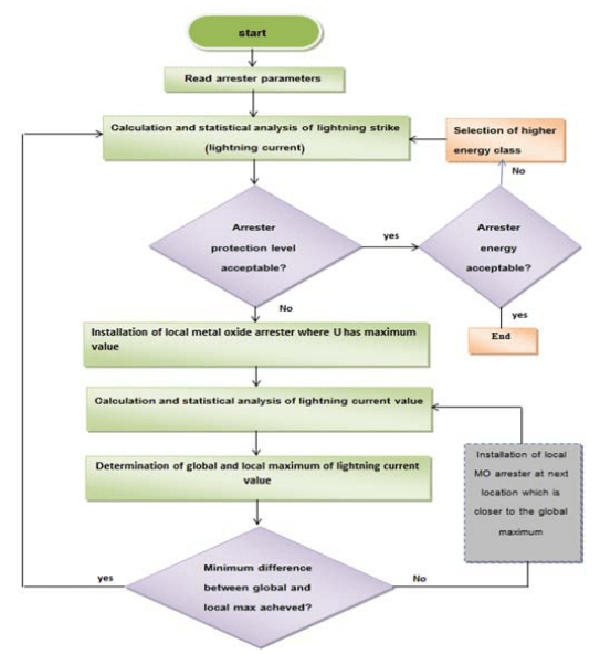
A 735kV transmission system with two T.L arresters located at the sending and the receiving ends of the line feeds a load (8MW) through a 16.093 Km T.L as given in Fig.3. Over the system a lightning surge of (10kA,20kA,30kA) was tempted and the simulation results were carried out by using MATLAB software environment.
Fig. 3. Proposed model
Algorithm flowchart template
In order to fulfil the scope of this work, the development process ode23t(mod/Trapezoidal) simulation of a metal oxide surge arrester on a 735 kV T.L is applied. The process flow of the modelling system with a details explanation is illustrated in Fig.4.
Fig.4. Flowchart of lightning metal oxide surge arrester on T.L
Results and discussion
Before the fault occurred, the simulation results showed the temporary putting-up in current at MOV1 and MOV2 after applying different lighting current values as illustrated in Fig.9 and Fig.10. In addition to the temporary increase in both arrester’s voltages. After fault at time 0.03 sec, the two arrester’s behaviour as steady state conditions but the load voltage has been increased as compared with the load current that decreased.
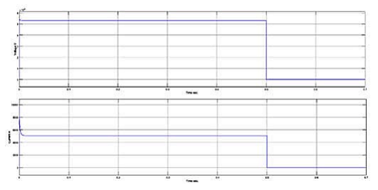
Ac current source (lightning source) At lightening surge (10kA) (Ac surge) Fig. 5-6 represents the relationship between voltage and current with respect to time at MOV1and MOV2.
Fig.5. Voltage and current waveforms vs time at MOV1 waveforms at MOV2.
Fig.6. Voltage and current waveforms vs time at MOV2.
Fig. 7 represents the relationship between voltage and current with respect to time at load.
Fig.7. Voltage and current waveforms vs time at Load
Fig.8. Voltage and current waveforms vs time at MOV1.
Fig.9. Voltage and current waveforms vs time at MOV2.
DC current source (lightning source) At lightning surge (10kA) (DC surge)
Fig. 8-9 represent the relationship between voltage and current with respect to time at MOV1and MOV2.
Fig. 10 represents the relationship between voltage and current with respect to time at load.
At lightning surge (10kA) (pulse surge) Fig. 11-13 represents the relationship between voltage and current with respect to time at MOV1and MOV2.
Fig.13 represents the relationship between voltage and current with respect to time at load.
Fig.10. Voltage and current vs time waveforms at load.
Fig. 11. Voltage and current waveforms vs time at MOV1.
Fig. 12. Voltage and current waveforms vs time at MOV2.
Fig. 13. Voltage and current vs time waveforms at load
Before the breaker (fault) switch is open i.e. before the fault occurred time the current passed into MOV1and MOV2 and no current appeared at load because the arresters (MOV1&MOV2) behaviour as non-linear resistance, in this case they behave as low resistance and the lightning current (10 KA) passed through them to the ground, no current signal appeared at load for all causes (AC, DC and Pulse) current surge.
Conclusions
After applying many different current sources on T.L many cases are appeared and they gave various conclusions as follows: From AC current source Fig. 5 and 6 show that after fault accrued, the voltage at MOV1 was lower than that at MOV2, but the current at MOV1 was higher than the current at MOV2. Fig. 8 and 9, show that after fault accrued, the voltage at MOV1 is approximately equal to the voltage at MOV2, and the current at MOV1 and MOV2 settled at zero. For the impedance of T.L, the current rating of the arrester and discharge voltage are 10KA and 30KV. This work will give and help the knowledge about the overvoltage of the protection system for T.L supported by the surge arrester. DC and pulse surges gave voltage at MOV1 higher than that generated by AC surge. AC surge gave voltage at MOV2 higher than that generated by booth DC and pulse surges. At 10KA (AC surge) Before fault occurrence, the voltage and current at MOV1 were lower than that at MOV2, but at load, the voltage reduced to zero and the current jumped instantaneously to (5250e7 ) due to the effect of impedance. The peak impulse voltage of the load current when the breaker has been closed appeared approximately equal for AC, DC and pulse surges.
Acknowledgments: We would like to thank our affiliation with the northern technical university (NTU) for supporting us in our work.
REFERENCES
[1] Gaurav S, Anshul M. Simulation of Compensated T. L Protection from Lightning by Using Matlab. IJERT. 2015; 4 (5): 146-149. [2] Chaitrashree SR, Sahana S, Rajalakshmi PM, Noor A. Analysis of the Use of Surge Arresters in Transmission System Using MATLAB/Simulink. IJAREEIE. 2016; 5(3):1428-1434. [3] M. G. Comber, S.F. LaCasse, R.M. Reedy, “Lightning Protection of T.Ls with Polymer-Housed Surge Arresters”, presented at EEI T&D Meeting Palm Beach, FL May 18, 1994. [4] S Satyanarayana, S.Sivangaraju, “Electric Power Transmission and Distribution” Pearson Education India, 2008. [5] Jaroszewski M, Pospieszna J, Ranachowski P, Rejmund F. Modeling of Overhead Transmission Lines with Line Surge Arresters for Lightning Overvoltages. Application of Line Surge Arresters in Power Distribution and Transmission Systems, Cavtat .2008;18(1):120-131 [6] Nangkyuthini K. Lightning Performance of Medium Voltage T.L Protected by Surge Arresters. An International Journal of Scientific Engineering and Technology Research. 2008; 3(16) :3362-3367. [7] Moe MS, Naung CW. T Lightning Performance of Medium Voltage T.L Protected by Surge Arresters International Journal of Research Publications.2014;3(16):3362-3367 [8] Sanketa S. Lightning Phenomenon, Effects and Protection of Structures from Lightning. IOSR-JEEE. 2016; 11(3): 44-50. [9] Santosh BK, Rajan HC. MATLAB/SIMULINK Simulation Tool for Power Systems” International Journal of Power System Operation and Energy Management. 2011;1(2): 2231 4407 [10 ] Safwan AH, Farah IH, Ali NH. Pitch Angle Control of Wind Turbine Using Adaptive Fuzzy-PID Controller. EAI Endorsed Transactions on Energy. 2020; 7 (28): 1-8 [11] Safwan AH, Ali NH, Ghanim MH. Automated irrigation system based on soil moisture using arduino board. Bulletin of Electrical Engineering and Informatics.2020 ; 9(3): 870-876. [12] Ali NH, Safwan AH, Rasha AM. Photovoltaic Modeling and Effecting of Temperature and Irradiation on I-V and P-V Characteristics. International Journal of Applied Engineering Research. 2018; 13(5): 3123-3127. [13] Ali NH, Safwan AH, Ahmmed GA. Photovoltaic-Battery System Tested under Sun Irradiance. LJER. .2018; 18( 2):65- 75. Ali NH, Safwan AH, Mohammed AI. Power Factor Correction [14] of AC to DC Converter Using Boost Chopper. J Appl Sci Eng. 2018; 13 (8): 6440-6445. [15] Rasha AM, Ali NH, Bashar MS. Partial discharge measurement in solid dielectric of H.V Cross-linked polyethylene (XLPE) submarine cable. Indonesian Journal of Electrical Engineering and Computer Science.2020; 17(3): 1578-1583.
AUTHORS: Ali N. Hamoodi, Northern Technical University (NTU), E-mail: ali_n_hamoodi@ntu.edu.iq. Rasha A. Mohammed, Northern Technical University (NTU), Email: rasha8479@ntu.edu.iq. Bashar M. Salih, Northern Technical University (NTU), E-mail: basharms_tecm@ntu.edu.iq.
Source & Publisher Item Identifier: PRZEGLĄD ELEKTROTECHNICZNY, ISSN 0033-2097, R. 99 NR 2/2023. doi:10.15199/48.2023.02.21
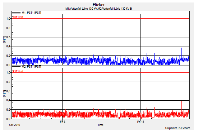
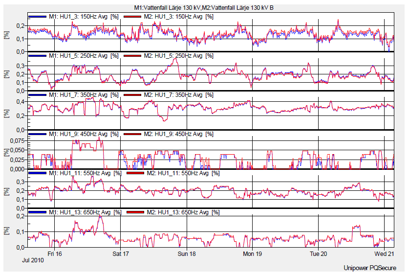
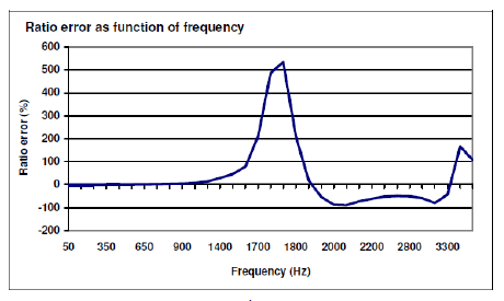
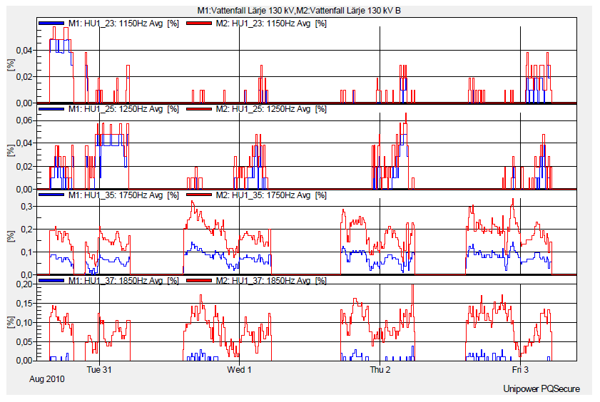
Published by Jonny CARLSSON – Unipower AB, David HOLMBERG – AB Vattenfall, Jan ÖSTLUND – ABB AB
Abstract A method of real-time calibrating the voltage signal from the Capacitive Tap on an ABB Current Transformer using Unipowers ‘UP-2210R/ABB Capacitive tap Module’ has produced accurate results of unbalance, harmonics and transients with no limitation in bandwidth. The method is to be preferred prior to measurements directly on the inductive VT since the capacitive tap eliminates the problem of limited frequency response on inductive VTs.
Another advantage of the method is that installation can be done without interrupting the power distribution.
Purpose
The purpose of this project is to evaluate a new technology for measurements on the capacitive tap where harmonics, relative and absolute, unbalance and transients can be measured correctly.
Background
Inductive and Capacitor Voltage Transformers do not reproduce harmonics in an accurate manner. Limited bandwidth changes the waveform at the transformer output causing harmonics to be amplified or attenuated.
Inductive voltage transformer
Capacitor voltage transformer
The charts below show an approximate overview of the bandwidth for inductive VTs and CVTs. In many substations there are capacitor tap outputs that can be used for high bandwidth measurements. A good example is the capacitive tap available on ABB current transformers. The bandwidth is similar to the C divider.
.
In the paper ‘Problems of Voltage Transducer in Harmonic Measurement’ Xiao, Hu and Deng describe the method of using the capacitive taps in Current Transformer bushings for relative harmonic measurements. The drawback of the recommended method is though that this voltage signal has no absolute reference and is floating/fluctuating over time and can therefore not be used for anything else than relative harmonics.
Project Background
At the interconnection points between Vattenfall, the largest sub-transmission and distribution company in Sweden and Banverket, Swedish railway operator, static converters are used for producing 16 2/3 Hz. Both Banverket and Vattenfall are interested in measuring power quality accurately in these points.
A joint project between Vattenfall, ABB and Unipower was therefore formed with the purpose of evaluating a new technique for PQ measurements conducted on an ABB current transformer ASEA IMBD145 in Gothenburg. The bandwidth of capacitive tap on this transformer is approx 1 MHz with a tangent delta of 0.025%-0.030% at 50 Hz.
Technical setup
Measurement techniques using the capacitive tap on the Current Transformer exist already today. The advantage is a very high frequency bandwidth. The drawback is that the signal is fluctuating quite a lot over time so measurement can only be relative, not absolute. Unbalance is a parameter impossible to measure on a floating signal and also the exact magnitude of transients registered will not be known. These parameters are usually of highest concern.
Thanks to modern signal-processing technique there is a new possibility available. Unipower AB producing PQ meters has specifically designed and equipped one of their high-end PQ meters with a set of extra voltage inputs (reference) with the purpose of real-time calibrating the high band-width voltage signal from the capacitive tap. The capacitive tap signal is calibrated continuously using a high accuracy, low band-width signal from either an inductive VT or CVT.
The result is a high band-width signal with absolute reference producing correct absolute harmonics, voltage, unbalance and transient recordings where measurements earlier were not possible. In addition the technique is cost effective since it is using the existing capacitive taps on the transformers already installed.
.
The Voltage transformer ASEA EMFC 145 has got an expected frequency response that is same as ABB EMF 145, see below picture:
Frequency response of inductive VT
This means that the result from the capacitive tap and from the Reference meter (Inductive VT) is expected to be the same up to approx 25th harmonic. Around 35th-40th harmonic the signal from the Inductive VT is expected to be amplified approx five times due to resonance.
Test results – Voltage measurements
To verify that the measurements on the Capacitive tap is calibrated correctly the two meters are plotted in the same diagram. Picture below shows that Capacitive Tap (blue) vs. Inductive VT (red) are correlating. This confirms that the on-line calibration of the signal from the capacitive tap is working accurately.
Capacitive Tap (blue) vs. Inductive VT (red)
Test results – Unbalance
For Unbalance the measurement result between the two meters are about the same. There is a small difference, about 0.05% that is within the accuracy requirements of IEC 61000-4-30 Class A. See picture below.
Capacitive Tap (blue) vs. Inductive VT (red)
Test results – Flicker
For Flicker the measurement result between the two meters are the same.
Capacitive Tap (blue) vs. Inductive VT (red)
Test results – Transients
During the test period there were few transients. The expected result was however confirmed. The Inductive VT was supposed to attenuate high bandwidth signals. Picture below show a transient captured at the capacitive tap. Since the amplitude was rather low the signal on the Inductive VT was attenuated and below the transient threshold level set at 30% deviation. The transient measured below correlate to a capacitor switching in the station. The time of the switching is 2010-10-15 6:15:26 according to Vattenfalls log (daylight saving) and the registered transient is at 2010-10-15 05:15:24,50 (standard time).
.
Next picture shows the same transient, but with fundamental subtracted:
.
Test results – Harmonics
The low order harmonics are as expected to be similar between the capacitive tap and inductive VT, see below:
Capacitive Tap (blue) vs. Inductive VT (red)
Difference on 3rd harmonic is 0.02%. Signal from capacitive tap is slightly lower. Difference on 5th harmonic is 0.01%. Signal from capacitive tap is slightly higher. H7, no significant difference. H9, no significant difference. H11, no significant difference. H13, no significant difference.
Up to the 25th harmonic there is no significant difference between the capacitive tap and the inductive VT. However on the 35th harmonic the signal from the inductive VT is approx +150% to 200%, and on 37th harmonic the difference is at its maximum and the signal from the inductive VT is approx +500% as compared with the signal from capacitive tap, see picture below. This is the expected behavior caused by resonance in the VT. The resonance points of the inductive VT can vary between different transformers but a typical frequency response can be seen below.
Frequency response of inductive VT
Capacitive Tap (blue) vs. Inductive VT (red)
Conclusion
The method of real-time calibrating the voltage signal from the Capacitive Tap using Unipowers ‘UP- 2210R/ABB Capacitive tap Module’ instrument has produced accurate results of absolute voltage, voltage unbalance, harmonics and transients with no limitation in bandwidth. The method is to be preferred prior to measurements directly on the inductive VT since the capacitive tap eliminates the problem of frequency response on inductive VTs.
Another advantage of the method is that installation can be done without interrupting the power distribution.
Published by Wesco | Anixter, Wesco International.
What are harmonics?
In an electric power system, a harmonic is a voltage or current at a multiple of the fundamental frequency of the system. Harmonics can best be described as the shape or characteristics of a voltage or current waveform relative to its fundamental frequency. When waveforms deviate from a sinewave shape, they contain harmonics.
Harmonic frequencies in the power grid are a frequent cause of power quality problems, resulting in increased heating in the equipment and conductors, misfiring in variable speed drives and torque pulsations in motors.
What causes harmonics?
AC electrical loads are referred to as either linear or non-linear, depending on how they draw current from the mains power supply waveform. With a linear load, the relationship between the voltage and current waveforms are sinusoidal and the current at any time is proportional to the voltage; this is known as Ohm’s law. Examples of linear loads include transformers, motors and capacitors.
With a non-linear load, the current is not proportional to the voltage and fluctuates based on alternating load impedance, meaning the current it draws does not have the same waveform as the supply voltage. Non-linear loads draw currents in abrupt short pulses. These pulses distort the current waveforms, which in turn generates harmonics that can lead to power problems affecting both the distribution system equipment and the loads connected to it. Examples of non-linear loads include rectifiers, variable-speed drives and electronic devices like computers, printers, TVs, servers and telecom systems that use switched-mode power supply (SMPS) power conversion technologies.
What are the consequences of harmonics?
A power system’s ability to perform at optimal levels is compromised when harmonic distortion enters the system. Harmonics create inefficiencies in equipment operations due to the increased need for power consumption. The increase of overall current required creates higher installation and utility costs, overheating and decreased profitability.
How can you reduce harmonics?
A few of the most popular ways to control harmonics include:
1. Trying to reduce the harmonic currents produced by the load. Adding a line reactor or transformer in series will significantly reduce harmonics, as well as provide transient protection benefits.
2. Adding filters to either siphon the harmonic currents off the system, thereby blocking the currents from entering the system in the first place, or supply the harmonic currents locally. For example, adding a shunt filter short-circuits harmonic currents as close to the source of distortion as practical. This keeps the currents out of the supply system. The shunt filter is a popular filter choice because it is cost-effective and can correct the load power factor while also removing the harmonic current.
3. Modifying the frequency response of the system with filters, inductors or capacitors. Active filters work by electronically supplying the harmonic component of the current into a non-linear load.
4. Providing transformer connections, which can reduce harmonic currents in three-phase systems.
5. Changing the capacitor size. This is often one of the least expensive options for both utilities and industrial customers.
Published Vijayshree G1, Sumathi S2, RNSIT, Bangalore,Karnataka,India(1). RNSIT, Bangalore,Karnataka, India(2)
Abstract – This paper proposes a power system network modeled using a microgrid, integrated with wind and solar photovoltaic (PV) resources, along with the battery energy storage system (BESS) connected to the three-phase grid feeding the linear and nonlinear load. The simulation is carried out with unit vector and instantaneous reactive power control algorithm for series and shunt active power filter respectively. The power quality improvement is analyzed for the voltage sag, swell, and harmonics for system with load variation and without load variation. The performance analysis is based on voltage & current THD, voltage & current RMS, and power and power factor analysis. The THD for comparison is represented in form of bar chart to show the effective performance of control algorithm proposed using PWM method and hysteresis controller.
Streszczenie. W artykule zaproponowano modelowanie sieci elektroenergetycznej za pomocą mikrosieci zintegrowanej z wiatrowymi i słonecznymi źródłami fotowoltaicznymi (PV) wraz z bateryjnym systemem magazynowania energii (BESS) podłączonym do sieci trójfazowej zasilającej obciążenie liniowe i nieliniowe. Symulacja prowadzona jest za pomocą wektora jednostkowego i algorytmu regulacji mocy biernej chwilowej odpowiednio dla filtru mocy czynnej szeregowego i bocznikowego. Poprawa jakości energii jest analizowana pod kątem zapadów, wzrostów napięcia i harmonicznych dla systemu ze zmiennym obciążeniem i bez zmiennego obciążenia. Analiza wydajności opiera się na THD napięcia i prądu, wartości skutecznej napięcia i prądu oraz analizie mocy i współczynnika mocy. THD dla porównania przedstawiono w postaci wykresu słupkowego, aby pokazać efektywne działanie algorytmu sterowania zaproponowanego przy użyciu metody PWM i regulatora histerezy. (Poprawa jakości energii elektrycznej w systemie generacji rozproszonej w warunkach zmiennego obciążenia z wykorzystaniem PWM i regulatora histerezy)
Keywords: microgrid, distributed generation, power quality, UPQC Słowa kluczowe: mikrosieci, rozproszone źróda energii, PWM
Introduction
Power quality (PQ) is used to assess and maintain the good quality of power at different levels (generation, transmission, distribution, and utilization) of the AC electrical power system. Power quality has become a challenging area of research in electrical engineering. Power quality is a combination of current and voltage quality. The voltage or current deviation from the ideal value is the disturbance of power quality. However, distinguishing between the voltage and current disturbances in the power system is difficult because for different customers different event leads to different disturbances. Therefore, in general, power quality is related to disturbances in voltage, current, frequency, and power factor. The electrical network considered for power quality assessment includes a three-phase programmable source connected to a microgrid with wind and solar PV resources along with battery storage. The system is connected to the non-linear load and linear load for power quality analysis. In [1] author explains generalized integrator controller which provides unity power factor (UPF) operation, load balancing, harmonics mitigation, and reactive power compensation for three phases single-stage grid interfaced solar energy conversion system. Different methods of analysis that describes the harmonic behavior of the electrical network and these data are reported to provide suitable mitigation strategies in a real-time operation is explained in [2]. The author in [3] explains the implementation of distributed generation operated for nonlinear and unbalanced load with different source conditions using enhanced Instantaneous Power Theory. The use of renewable energy sources has different environmental benefits and is also economical when compared with the traditional source of power generation [4]. The integration and control of renewable energy in electric power systems is mathematically modelled in [5] .In [6] ,a modified p-q theory-based control that implements a solar photovoltaic (PV) array integrated unified power quality conditioner (PV-UPQC-S) for analysis of the steady and dynamic performance of the system is explained. The paper [7] proposes a three-phase transformer less Hybrid Series Active Filter (THSeAF) in combination with SRF and PQ theory to provide suitable mitigation for power quality issues. [8] explains about the stationary and non-stationary power quality disturbance which is mitigated using variational mode decomposition (VMD) and decision treebased detection method which is capable of accurate detection, estimation, localization, and classification of all kinds of PQ disturbances in both noisy and noise-free cases. [9] explains how fluctuation in photovoltaic (PV) power plants affects the power quality and stability of the grid along with the increasing penetration of PVs. The addition of an energy storage system resolves this issue. The importance of battery parameter state of charge is taken care of to ensure the stability of the energy storage system. In [10], different positions of UPQC placement for better performance are analyzed. A Synchronous reluctance generator is used as an input to feed linear and nonlinear loads with an adaptive neural network-based control algorithm to improve power quality which mitigates some power quality problems such as harmonic suppression, and load balancing, reduction in frequency variation and voltage regulation[11]. Passive and active filters in providing power quality compensation, the advantages and disadvantages of both types of filters are explained and justify that the active power filter is more advantageous [12].
Problem formulation
The three-phase voltage source of 415V, 50 Hz is integrated with a Microgrid designed with solar and wind generation connected to linear and nonlinear load . The magnitude of the voltage at the microgrid is maintained the same as the supply voltage as it is connected in parallel. The supply voltage is observed to be 229.2 volts phase to phase as shown in figure 1, at t=0s to t=0.1s. The voltage sag of 0.6 pu is introduced at t= 0.1s to t= 0.25s whose magnitude is reduced to 138V as indicated in figure 1, at t= 0.1s to t= 0.25s.Its corresponding RMS voltage is shown in figure 2. The power system is connected to a nonlinear load of a three-phase bridge rectifier with R= 40Ω and L=1e-4 H through a transmission line of resistance 0.002 ohms and inductance of 1e-5 H. At t=0.02 s, the linear load is added to the system to analyze the effect of a sudden change in load on the power system considered. The decrease in voltage and increase in current from t= 0.02s to t=0.16s, due to the addition of load is shown in figure 3 and figure 4.
Fig.1. Voltage waveform without UPQC Compensation
Fig.2. RMS voltage (sag) without UPQC compensation due to a change in load
Fig.3. Voltage waveform to indicate a decrease in voltage due to a change in load
Fig.4. Current waveform to indicate an increase in current due to a change in load
The RMS current waveform for variation in load is as shown in figure 5 where the load is added at t=0.02 s to t= 0.16s. The load is removed at t=0.16s, and hence the magnitude of the current decreases at t=0.16s. At t= 0.1 s, the voltage sag of 0.6 pu is introduced which indicates the reduction in power at that instant as shown in figure 6. It is observed in figure 7, that the power factor without UPQC compensation is 0.94.
Fig.5. RMS Current waveform to indicate an increase in current due to a change in load
Fig.6. Waveform representing power before UPQC compensation
Fig.7. The waveform of Power factor without UPQC compensation
Design of unified power quality controller (UPQC)
In view of improving the system performance by mitigating the defined power quality issue in section 2, UPQC is designed with a unit vector algorithm for series active power filter (APF) and Instantaneous reactive power theory for shunt active power filter. The gate pulse is generated using the PWM technique in series APF and PWM and the hysteresis controller in the shunt active filter. The MATLAB simulation model designed for the defined power system network is shown in figure 8.
Three-phase voltage source in parallel to the microgrid at the supply terminal is connected to a three-phase load (both linear and nonlinear) through the transmission line. The UPQC comprising of series and shunt compensator is as shown in figure 8. The series active filter is designed using a unit vector control algorithm. The single phase input is fed to the phase-locked loop with the gain of 0.005 to obtain the value of wt. The three-phase voltage is derived by using the equation (1) – (3) which is then compared with the supply voltage to determine the error in voltage that derives the switching signals using the method of pulse width modulation.
Fig.8. A simulation model for Power system network with UPQC
.
The series active filter is connected to the supply terminal using three phases linear transformer with 12 terminals with three phases rated power of 10e6VA, with 50 Hz frequency. The winding RMS voltage is set to 100V, R= 0.002pu and X= 0.00005 pu.
The design of shunt APF is done using instantaneous reactive power theory (IRPT) with two different control algorithms for the generation of switching signals. One uses a PWM controller and the other uses a hysteresis controller. The IRPT is designed using supply voltage and load current. The reference current is obtained using supply voltage, load current, and control signal obtained using a PI controller. The reference current is obtained using the equation (4) – (9)
.
The series and shunt compensation is provided by using a MOSFET-based universal bridge inverter connected along with the interfacing inductor of 4e-3 H. The simulation results after providing UPQC compensation for the problem formulated are shown in figure 9. In figure 9, at t= 0.05s and t=0.15s, with a magnitude of voltage 231.6 V. Its corresponding RMS component of voltage is shown in figure 10.
Fig.9. Waveform of voltage after UPQC compensation
Fig.10. The waveform of RMS voltage after UPQC compensation
Fig.11. Waveform of current after UPQC compensation
The current waveform is as indicated in figure 11. The magnitude of current is 14.54 A at t= 0.02s to t=0.16s. At t=0.16s the linear load is removed and hence the magnitude of the current is reduced to 12.3A. After UPQC compensation the power waveform is as shown in figure 12. The magnitude of power is 1543 W at t= 0.02s to t= 0.16s. As the load is removed at t=0.16s, the power magnitude also reduces to 1333 W. The power factor after UPQC compensation is as shown in figure 13, where the power factor is improved to 0.98 compared to 0.94 without UPQC compensation. As per IEEE standards 519-1992: For general distribution system, current distortion limits obtained by the simulation performed lie within the limit.
Fig.12. The waveform of Power after UPQC compensation
Fig.13. Waveform of Power factor after UPQC compensation
The comparison of simulation output obtained from PWM and hysteresis controller for system without variation in load and with variation in load for different magnitudes of voltage sag and swell and harmonic orders are as tabulated in table 1 to table 6.
Table 1. THE MAGNITUDE OF FUNDAMENTAL COMPONENT OF VOLTAGE AND CORRESPONDING THD FOR VOLTAGE SAG AND SWELL WITHOUT LOAD CHANGE.
.
Table 2. THE MAGNITUDE OF FUNDAMENTAL COMPONENT OF CURRENT AND CORRESPONDING THD FOR VOLTAGE SAG AND SWELL WITHOUT LOAD CHANGE.
.
Table 3. THE MAGNITUDE OF FUNDAMENTAL VOLTAGE COMPONENT AND CORRESPONDING THD FOR VOLTAGE SAG AND SWELL WITH LOAD CHANGE.
.
Table 4. THE MAGNITUDE OF FUNDAMENTAL COMPONENT OF CURRENT AND CORRESPONDING THD FOR VOLTAGE SAG AND SWELL WITH LOAD CHANGE.
.
Table 5. THE MAGNITUDE OF FUNDAMENTAL COMPONENT OF CURRENT AND CORRESPONDING THD FOR HARMONICS
.
Table 6. THE MAGNITUDE OF FUNDAMENTAL COMPONENT OF VOLTAGE AND CORRESPONDING THD FOR HARMONICS.
.
Conclusion
The aim of power quality improvement is to provide pure sinusoidal voltage and current to the consumers. The problem formulated includes the addition of load at the distribution end, introducing voltage sag, swell, and harmonics of a different order which is as shown in figure 1 – figure 4.
The above-defined power quality-related issues are mitigated using a combination of shunt and series active power filters called UPQC with PWM and hysteresis controller as shown in figure 9-figure 11.The bar chart representation of THD for voltage and current without UPQC, with UPQC PWM and UPQC Hysteresis is shown in figure 14 –figure17. It can be concluded that PWM controller gives good performance when compared to hysteresis controller. The power and power factor, corresponding RMS voltage, and current is analyzed to show the effectiveness of UPQC designed to improve the power quality.
Fig.14. Voltage THD for power system without variation in load
Fig.15. Current THD for power system without variation in load
Fig.16. Voltage THD for power system with variation in load
Fig.17. Current THD for power system without variation in load