Published by Paweł WĘGIEREK, Michał LECH, Lublin University of Technology, Faculty of Electrical Engineering and Computer Science
Abstract. The article presents the detailed construction and capabilities of a research station for the diagnosis and testing of vacuum interrupters used in medium voltage electrical switching devices. The correct functioning of the stand has been confirmed by conducting a number of tests on the electrical strength of the MV switchgear vacuum interrupter type HVKR 24/400.
Streszczenie. W artykule przedstawiono szczegółową budowę oraz możliwości stanowiska badawczego służącego do diagnostyki oraz badań komór próżniowych wykorzystywanych w elektroenergetycznej aparaturze łączeniowej średniego napięcia. Poprawność funkcjonowania stanowiska potwierdzono przeprowadzając szereg badań wytrzymałości elektrycznej próżniowej komory rozłącznikowej SN typu HVKR 24/400. (Stanowisko badawcze przeznaczone do badań i diagnostyki komór próżniowych średniego napięcia).
Power engineering is a field of economy developing at a surprisingly fast pace. Many factors influence this process. One of them is the constantly growing number of new electricity consumers, and thus increasing the power required in areas that have not been urbanized before. According to the Transmission System Development Plan, by 2030 [1] the total net electricity demand in 2040 will be 204.2 TWh with 159.9 TWh in 2020.
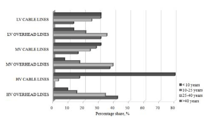
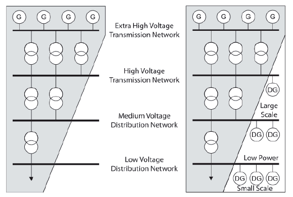
Another factor in the development of the Polish power industry is its current technical condition (Fig. 1). Outdated elements of the power infrastructure force the investments of power companies related to various types of modernizations [2, 3]. A particular problem is visible in the area of high and medium voltage overhead lines, over 75% of which were built more than 25 years ago [4]. MV power lines are one of the most important elements of the distribution system for both technical and economic reasons [5].
Fig.1. Age structure of selected elements of the polish power system [4]
Another factor enforcing the dynamic development of the power industry is a number of legal requirements imposing on power companies to improve their power supply conditions and to move away from equipment using environmentally harmful greenhouse gases [6-11].
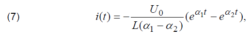
The above factors show that there is a strong need to develop new solutions among power equipment, mainly medium voltage. Many companies and scientific entities have faced this problem and developed pro-ecological equipment, using vacuum as an insulating medium.
One of such devices is the innovative EKTOS vacuum switch disconnector, which is the final result of the project entitled: “Development and implementation of an innovative closed cased overhead vacuum switch disconnector dedicated to intelligent medium voltage networks”, carried out by the Lublin University of Technology in consortium with EKTO Sp. z o.o. from Białystok as part of the activities of the National Research and Development Centre. This device is addressed to Distribution System Operators (DSOs) who want to improve the reliability of electricity supply in the areas they manage through investments in new technologies [12].
Methods for diagnosing vacuum conditions
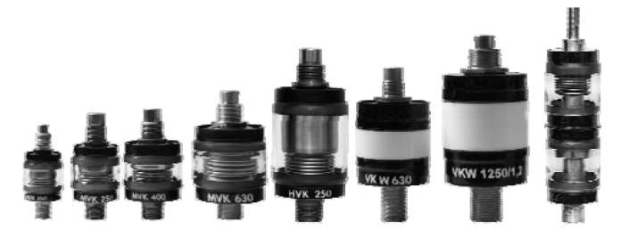
Equipment such as contactors, switches and disconnectors with installed vacuum interrupters are commonly used in the power industry. The ever-increasing number of such devices is directly related to the need for an effective diagnosis of the state of vacuum inside them. A number of existing diagnostic methods are used for this purpose to assess the proper functioning of medium voltage vacuum extinguishing interrupters in terms of dielectric strength. Examples of vacuum interrupters used in switchgear are shown in Figure 2.
Fig.2. Examples of vacuum interrupters used in switchgear [13]
The basic ones include: the Pening method and the Magnetron method [14, 15]. They consist of placing the tested chamber in a magnetic (strongly axial) field, and then applying a DC voltage of 10 ÷ 20kV to open contacts. According to the gas breakdown mechanism, due to the electric field created due to the applied voltage, electrons are emitted from the cathode moving towards the anode. Placing the chamber under test in the magnetic field changes the path of electrons motion into a spiral one, thanks to which the number of collisions with atoms and molecules of residual gas increases. The mentioned methods consist in recording the current of electron emission, which results from the collision ionization occurring in the chamber. In order to assess the vacuum condition, the characteristics determined for the new vacuum chamber must be known for further comparison.
Another method of diagnosing the state of vacuum is the static AC ignition voltage method [14, 16]. It consists in measuring the value of the jump voltage and then comparing it with the Pashen curve for a given chamber.
The static DC ignition voltage method, which is relatively simple, can also be used to check the correct operation of vacuum chambers. It consists in applying a certain voltage value to the chamber in the open state and then measuring the current value in the chamber and comparing it with the maximum allowable value [14, 17].
In high-frequency test systems, a frequently used method of diagnosing the vacuum condition is the method of AC current switching capability [14, 18], consisting in determining the ability to switch off the AC current, which clearly decreases at certain pressure values.
The Fowler-Nordheim dependence is often used for vacuum chamber tests [14, 19]. This method was called the emission current test method [14, 20]. The use of this method requires appropriate testing equipment, allowing the application of high DC voltage to the chamber, as well as measuring equipment enabling the measurement of currents at the microampere level.
A similar method to the one described above is the test method for emission currents with HF current surges [14, 17]. It consists in forcing a high current value of the frequency exceeding 1 kHz to flow through the chamber, which smoothes the contact surfaces of the chamber being diagnosed.
An interesting method of diagnosing the vacuum condition is the measurement of X-ray radiation [14, 18, 20]. The analysis uses the fact of proportionality of its intensity to the emission current. This method is characterized by a significant defect, consisting of interference from background radiation, which is greater than the radiation of the chamber under operating conditions, so that the results can be significantly disturbed.
Another method consists in measuring the arc voltage at direct current of 10A (DC arc voltage method) [14, 20]. This voltage increases its value while extinguishing the electric arc, while it decreases its value while developing new cathode spots associated with, among others with residual gas in the chamber. The higher the value of the peak voltage, the lower the pressure in the tested chamber.
The method based on measuring the value of the voltage initiating the micro-discharge and the voltage initiating the emission current, called the Vd/Ve method, uses the dependence about the inverse of these voltages in relation to the pressure inside the chamber [14, 21].
For vacuum chambers with external access to their screen, a method of measuring the screen potential can be used to assess the vacuum. It uses the phenomenon of changing the chamber screen potential under the influence of emitted electrons from the chamber contacts [14, 22].
Another method is the method of switching off low induction current, which consists in applying overvoltage impulses to the chamber’s contacts and using the phenomenon of power surges [14, 22].
The method of switching off capacitive current is implemented by breaking the circuit in which the capacitive current flows in the oscillating system [14, 22]. Then, the value of voltage appearing at the terminals of the tested chamber is used to assess the state of the vacuum.
There is also a diagnostic method of vacuum chambers based on the measurement of partial discharges that appear in the chamber during operation. However, the effectiveness of this method is visible at high pressures, which indicate complete leakage of the chamber [14, 22].
Test stand
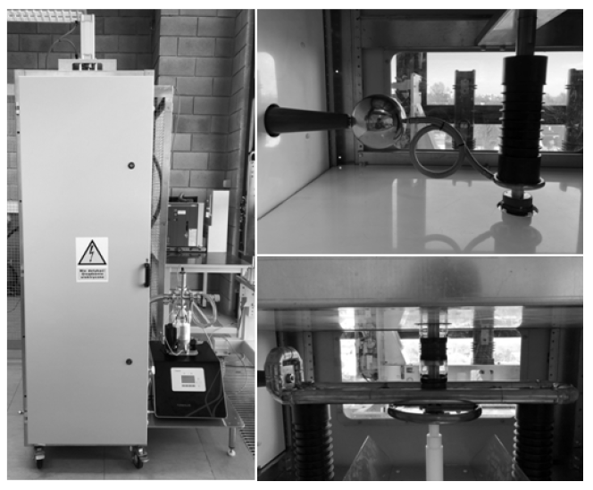
This test stand for the diagnosis and testing of vacuum interrupters used in medium-voltage switchgear has been designed and manufactured on the basis of a stable, mobile construction with a special platform used for the foundation of the vacuum pump set (Fig. 2). Inside the stand there is space for mounting the research object – medium voltage vacuum interrupter. The desire for a comprehensive study of the electrical strength of the vacuum interrupter is associated with the need to be able to change the contact distance in the appropriate range and with appropriate accuracy. In this test stand it was realized by mounting an extraction screw with a 1 mm pitch thread. Thanks to this, with the use of an appropriate reference scale, it is possible to set the inter-contact distance with the accuracy of 0.1 mm.
Fig.2. View of the test stand together with the method of test object assembly
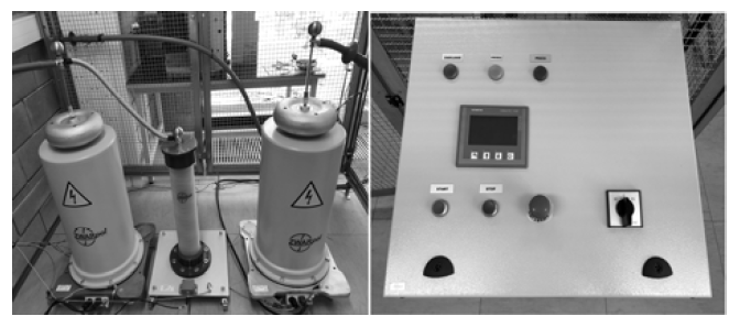
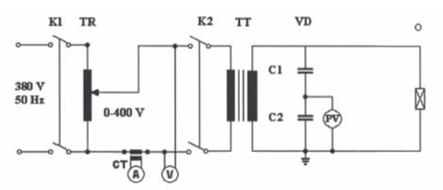
Power supply to the test stand is provided by means of YHAKXS 1x120mm2 power cable terminated with an angular connector head enabling quick and convenient connection of power supply to the test stand. The test set consists of three main elements: high voltage transformer, capacitive measuring divider and control panel (Fig. 3).
Fig.3 Test set with control panel
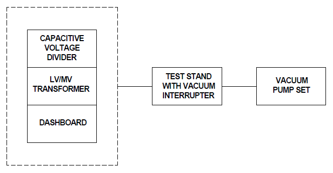
The nominal parameters of the kit are shown in Table 1. The schematic diagram of the complete test stand is shown in Figure 4.
An important element of the test stand is a vacuum set to obtain the appropriate pressure inside the vacuum interrupter to be tested. This is done by a set consisting of a turbomolecular and rotary vacuum pump operating at a capacity of 90 l/s.
Table 1. Rated parameters of the test set
.
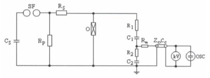
Fig.4. Block diagram of a complete test bench for testing and diagnostics of medium voltage vacuum interrupters
Research facility
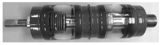
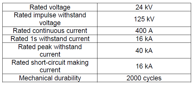
In order to verify the correct operation of the test stand, a test object was installed in it, which is the HVKR 24/400 vacuum disconnector interrupter (Fig. 5). Interrupters of this type are used in three-pole medium-voltage switch disconnectors operating in overhead power networks. Rated parameters of the interrupter are shown in Table 2.
Fig.5 Test facility: HVKR 24/400 vacuum interrupter
Table 2. Rated parameters of the HVKR 24/400 chamber
.
The above vacuum interrupter consists of two poles: mobile and fixed, with contacts made of a mixture of tungsten and copper at a ratio of 70% tungsten to 30% copper. An inseparable element of the interrupter is an elastic bellows enabling the movement of the moving pole, as well as a condensation screen catching conductive particles which, if deposited on the interrupter casing, would deteriorate its operating parameters.
Verification of the correctness of the position
Using the test stand described in this article, it is possible to diagnose the vacuum condition of the selected switch extinguishing interrupter. It is necessary to know its reference electrical strength characteristics and then to compare it with the obtained test results.
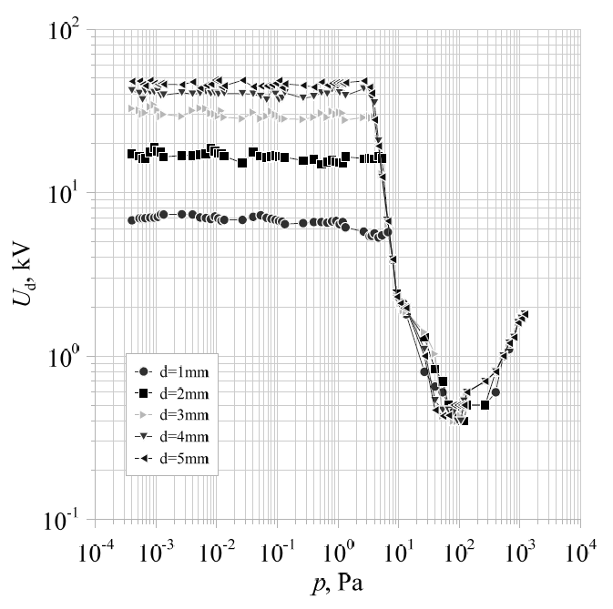
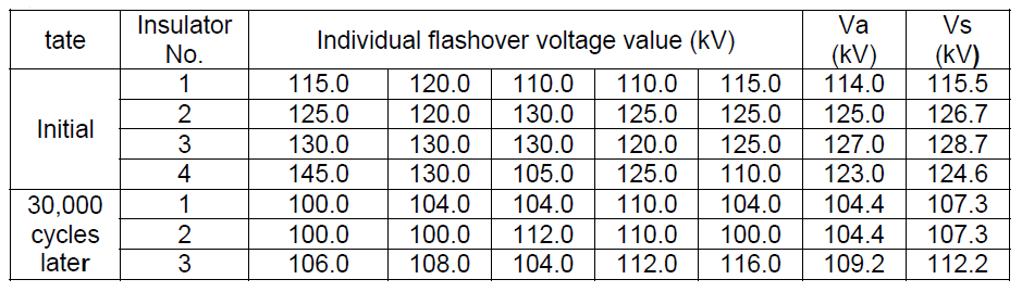
Verification of the correctness of operation of this method, called as a static AC ignition voltage method, was carried out in laboratory conditions for the contact distance in the range of 1 ÷ 5 mm for pressure from 4×10⁻⁴ ÷ 1.2×10³ Pa. The test results are presented in Figures 6 and 7.
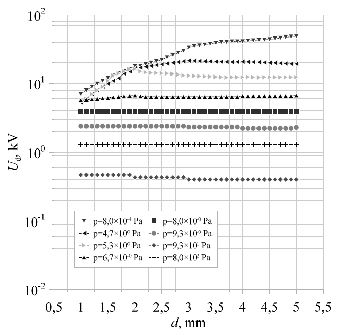
Fig.6 Relationship of breakdown voltage Udas a function of pressure p inside the vacuum interrupter under test
Fig. 7. The relation of the voltage breakdown Ud as a function of the contact distance d
When analysing the above characteristics, attention should be paid to the pressure range in which the dielectric strength of the inter-contact interval of the vacuum interrupter under test is kept constant (Figure 6). This creates a certain safety zone which guarantees the reliable operation of a given device with respect to the electrical strength of the vacuum interrupter installed in it. This situation occurs below a pressure of . 5×100 Pa. The recorded breakthrough voltages in this zone are listed in Table 3.
As the pressure in the tested interrupter increases, a sharp drop in strength is visible. Figure 7 shows the dependence of the breakthrough voltage of the tested vacuum interrupter on the contact distance for selected interrupter pressure values. For pressures between 8,0×10⁻⁴ ÷ 5.3×10⁻¹ Pa, the breakthrough voltage increases with the increase in the inter-contact distance. When the interrupter is further aerated, the characteristics are flattened. From the pressure value equal to 6.7×100 Pa, the contact distance did not influence the dielectric strength of the electrical interruption. A vacuum interrupter to be diagnosed, for which the measured value of dielectric strength would be within this range, would be diagnosed as defective.
Table 3. Values of breakthrough voltages recorded in the safety zone of the vacuum interrupter under test
.
Summary
The test stand presented in this article provides an opportunity to diagnose standard vacuum interrupters used in medium-voltage switchgear as well as to test them for improvement of operational parameters.
In order to verify the correct operation of the presented test stand, a number of tests were performed and graphical relationships between the selected parameters were obtained. On the basis of the obtained test results, it can be concluded that the stand described in the article was properly designed and made, and thus it is possible to use the static AC ignition voltage method.
The nearest research works will concern the improvement of electric parameters of vacuum interrupters by increasing the electrical strength of the inter-contact break, as well as limiting the negative effects related to the burning process of the electric arc of the inter-electrode space. The research will be supported by modern computer software enabling professional simulation of physical phenomena taking place in vacuum interrupters used in modern medium voltage electrical apparatus.
This work was supported by The National Centre for Research and Development and co-financed from the European Union funds under the Smart Growth Operational Programme (grant # POIR.04.01.04-00-0130/16).
LITERATURE
[1] Development plan for meeting current electricity demand for 2021-2030, Konstancin – Jeziorna, 2020 [2] Łukasik Z., Kozyra J., Kuśmińska-Fijałkowska A.: Monitoring of low voltage grids with the use of SAIDI indexes, Przegląd Elektrotechniczny, 10/2017, p.141-145 [3] Marzecki J.: Modernization and development directions of low and medium voltage rural network, Przegląd Elektrotechniczny, 2/2019, p. 67-70 [4] Power engineering, distribution and transmission, Polish Power Transmission and Distribution Associaton’s Report, Poznań, 2017 [5] Chojnacki A. Ł.: Comparative analysis of indicators and reliability properties of medium voltage overhead and cable power lines, Przegląd Elektrotechniczny, 11/2019, p. 26-30 [6] Konarski M., Węgierek P.: The use of Power restoration systems for automation of medium voltage distribution grid, Przegląd Elektrotechniczny, 7/2018, p. 167-172 [7] Montreal Protocol on Substances that Deplete the Ozone Layer, Montreal, 1987 [8] Kyoto Protocol to the UN Framework Convention on Climate Change, Kyoto, 1997 [9] Regulation (EU) No 517/2014 of the European Parliament and of the Council of 16 April 2014 on fluorinated greenhouse gases [10] Quality Regulation 2018 – 2025 for Distribution System Operators [11] Ordinance of the Minister of Economy of 4 May 2007 on detailed conditions of the power system operation [12] Węgierek P., Staszak S., Pastuszak J.: EKTOS – innovative medium voltage outdoor vacuum disconnector in a closed housing dedicated to the network smart grids, Wiadomości Elektrotechniczne, 11/2019, p. 21-25 [13] http://www.repo.itr.org.pl/energetyka/vc.html, access:18.06.2020r. [14] Chmielak W.: Review of methods of diagnostics of the vacuum in vacuum circuit breakers, Przegląd Elektrotechniczny, 2/2014, p.213-216 [15] Kuhl W., Schilling W., Schlenk W.: Messung des lnnendruckes in Vakuumschaltróhr, Vakuum-Technik 34. Jahrgang . Heft 2/85 Seite 34 bis 38 [16] Damstra G. C.: Pressure Estimation in Vacuum Circuit Breakers, IEEE ‘Trans. on Dielectrics and Electrical Insulation Vol. 2 No.2, April 1995 [17] Frontzek F.R., Konig D.: Measurement of Emission Currents Immediately After Arc Polishing of Contacts, IEEE Trans. on EI, vol. 28,No. 4, 1993, p. 700-705 [18] Frontzek F.R., Konig D., Methods for internal pressure diagnostic of vacuum circuit breakers, IEEE 18th ISDEIV – Eindhoven-1998, p. 467-472 [19] Kamarol M., Ohtsuka S., Hikita M., Saitou H., Sakaki M.: Determination of Gas Pressure in Vacuum Interrupter Based on Partial Discharge, IEEE Transactions on Dielectrics and Electrical Insulation Vol. 14, No. 3; June 2007, p. 593 – 596 [20] Walczak K., Janiszewski J., Mościcka-Grzesiak H.: Evaluation of internal pressure of vacuum interrupters based on dynamics changes of electron field emission current and X-radiation HV, Eng. Symp. Aug. 1999 [21] Ziyu Z., Shuheng D., Xiuchen J., Naixiang M., Liwen L., Huansheng S., Chongfang L.: Measurement of Internal Pressure of Vacuum Tubes by Micro-discharge and Emission Current XXIII-rd ISDEIV – Bucharest – 2008 [22] Damstra G.C., Merck W.F.H., Bos P.J., Bouwmeester C.E.: Diagnostic Methods for Vacuum State Estimation, IEEE 18th ISDEIV-Eindhoven-1998, p. 443-446
Authors: dr hab. inż. Paweł Węgierek, profesor uczelni, mgr inż. Michał Lech, Politechnika Lubelska, Wydział Elektrotechniki i Informatyki, ul. Nadbystrzycka 38A, 20-618 Lublin, E-mail: p.wegierek@pollub.pl, m.lech@pollub.pl.
Source & Publisher Item Identifier: PRZEGLĄD ELEKTROTECHNICZNY, ISSN 0033-2097, R. 97 NR 2/2021. doi:10.15199/48.2021.02.36
Published by 1. Yuly Bay, 2. Nikolay Ruban, 3. Mikhail Andreev, 4. Alexandr Gusev, Tomsk Polytechnic University. ORCID. 1. 0000-0001-9928-408X, 2. 0000-0003-1396-9104, 3. 0000-0002-6420-4374, 4. 0000-0003-0814-2356
Abstract. The penetration of renewable energy sources (RES) into the electricity supply is gaining popularity all over the world, including countries that have large oil and gas reserves, since only the development of alternative energy will help avoid regression and take a green path development, reducing the damage to the environment. According to estimates of the International Energy Agency (IEA), the capacity of RES units built in China in 2016 was 34 GW, and Australia is one of the world leaders in the photovoltaic power plants installation, the share of which in the Australian electricity production exceeds 3%. It should be noted, that the final power generation capacity and stability are stochastic (probabilistic) in nature. Unlike the classical type generator, the output RES characteristics depend on the geographical features of the installation area, the season, and prevailing winds. Risks associated with inaccurate knowledge of the cumulative distribution function (CDF) describing these sources, as well as environmental uncertainties, are the reasons why it is more difficult for distribution network operators (DNO) to take RES into account in the power balance calculations. The wind speed CDF clarification can provide significant assistance in predicting the RES power production.
Streszczenie. Według szacunków Międzynarodowej Agencji Energetycznej (IEA) moc jednostek OZE wybudowanych w Chinach w 2016 roku wyniosła 34 GW, a Australia jest jednym ze światowych liderów w instalacji elektrowni fotowoltaicznych, której udział w australijskiej produkcji energii elektrycznej przekracza 3%. Należy zauważyć, że końcowa moc i stabilność wytwarzania energii ma charakter stochastyczny (probabilistyczny). W przeciwieństwie do generatora typu klasycznego, charakterystyka wyjściowa OZE zależy od cech geograficznych obszaru instalacji, pory roku i dominujących wiatrów. Ryzyko związane z niedokładną znajomością skumulowanej funkcji dystrybucji (CDF) opisującej te źródła, a także niepewności środowiskowe powodują, że operatorom sieci dystrybucyjnych (DNO) trudniej jest uwzględnić OZE w obliczeniach bilansu mocy. Wyjaśnienie prędkości wiatru CDF może zapewnić znaczącą pomoc w przewidywaniu produkcji energii z OZE. (Analiza statystyczna rozkładów probabilistycznych prędkości wiatru do oceny energetyki wiatrowej w różnych regionach)
Keywords: power system, wind speed time series, probability density function, cumulative distribution function. Słowa kluczowe: energetyka wiatrowa, rozkład statystyczny.
Introduction
The structure and principles of power system management are becoming more and more complicated. Over the past 15 years due to the insufficient capacity of traditional generation sources, in most developed countries, for reasons of ensuring energy, environmental safety, etc., preference is given to RES, which is being actively introduced in China, Europe and the United States, and the total generated capacity is approximately 2195 GW. Due to this, the total RES capacity is expanding, which leads to an increase in power system stochastic processes.
In the classical cases, the electrical power system (EPS) is a «vertically» arranged system, where a number of operating factors and controlled variables are clearly defined and set within a specific way, established by the DNO [1]. However, in cases of renewable generation penetration, especially in large amount, there is a problem of discrepancy between the generated capacity and the electricity demand. Poor predictability associated with the current wind flow strength, which does not coincide in time with the required capacity, leads to mode dispatching problems. The RES, unlike traditional generators, restructuring EPS into a «vertical-horizontal» one [2], adding uncertainties in management that require further research and forecasting.
The ability and accuracy of forecasting is limited by the statistical information quality or methods of its processing. For example, in these works [3], deterministic methods were used to predict power generation, in order to represent RES as classical. In the articles [4], the probability distribution functions were selected for the input and output characteristics by the statistical analysis methods and testing by goodness of fit criteria. There are also studies devoted to the investigation of the power system units probabilistic characteristics, such as the expected value and standard deviation, the calculation of which contributes to the calculation of the optimal RES implementation capacity in order not to loss of steady state and transient stability.
The wind speed probability distribution approximation
The distribution law choice depends on many factors, including the specifics of the problem. To determine the estimated wind speeds of low frequency (dependence on the wind rose chart [5]), the maximum wind speeds possible in a particular area [6]), the main requirement is a reliable coincidence of empirical and theoretical distributions in the high-value range. The approximation itself as applied to the wind speed distribution was initially widely used for statistical extrapolation of the maximum wind speeds [7]. Subsequently, the approximation of the wind speed distribution by the Weibull and Weibull-Goodrich laws has become one of the most widely used [8]. Along with this law, the normal distribution law is often used, but a large sample size is required to reliably estimate the distribution parameters.
There are papers [9] that claim that the probability distribution is also well described by the lognormal distribution. The laws that can be used for modelling the wind speed, as well as their parameters, are given in the Table 1.
Table 1. Expressions of statistical distributions
.
where k – shape parameter, c – scale parameter, Г – gamma function, α,β,η – parameters of distributions, – normal distribution
The form of the distribution law also depends on the set of observations. In such situations, the distributions of the criteria statistics are often unknown, which is a frequent source of incorrect conclusions.
For optimal research, it is necessary to use several methods to determine the possible distribution law, even before using the goodness of fit criteria. Several well-known methods have been used to determine the various distributions parameters, out of which the method of moments, the graphical method, and the maximum likelihood method. In the case of using the graphical method, it has the advantage of simplicity, however, the accuracy of the input parameters estimating can be insufficient [10]. The likelihood method, on the contrary, has good accuracy, but to achieve it, it is required to use iterative methods [11]. The method of moments equates a certain number of statistical moments of the sample with the corresponding population moments [12]. The use of these methods (at least the maximum likelihood method and method of moments) usually implies that there is an assumption of the possible probability laws that are available in the wind time series. However, in the case of considering the unexplored wind time series, it is more logical to use the graphical or brute force method [13], with subsequent evaluation by several goodness of fit criteria.
The goodness of fit tests
The suitability of the chosen theoretical distribution for describing the empirical probability of a given meteorological argument is verified using the goodness of fit criteria. In this article, we will use Pearson’s chi-squared test [14] and Kolmogorov-Smirnov Goodness-of-Fit Test [15, 16], since the first of them is very sensitive to the dissimilarity of the values edges, the second allows us to more accurately assess the differences in the central regions.
Applying both criteria (with a given 5% significance level), the selected theoretical distribution function can be safely used for indirect calculations. For the measure of the difference between the theoretical and empirical distributions, Pearson takes the value X2 determined by the formula:
.
where n – the sample size, mi – the relative frequencies of the empirical distribution, pi– the corresponding theoretical probability densities, k – the gradations number.
Kolmogorov proposed another goodness of fit criteria, which, in contrast to the Pearson criterion, is based on a comparison of experimental and theoretical distributions integral laws.
As a measure of difference, A. N. Kolmogorov-Smirnov test uses the value:
.
where n – the sample size, D – corresponds to the upper bound (the largest value of the difference between the considered and the original sample) |F*(xi) – F(xi)| = δ(xi).
Input wind time series data
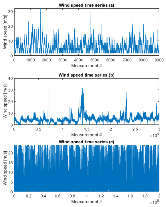
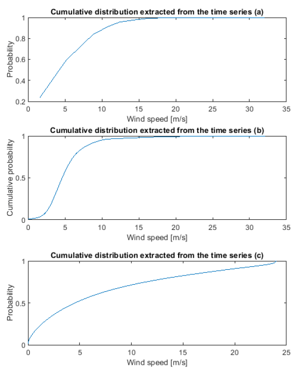
For the experiments, three samples of wind time series data with unknown CDF were taken. The sample size is between 9000 and 200000 volumes, depending on the example. The first sample (Fig. 1a) was taken from one of the graphical method experiments to study Weibul’s law parameters, and was randomly generated. The second time series is taken from the small-scale wind turbine power curve study (Fig. 1b) [17]. The third sample (Fig. 1c) is taken from the wind hourly NUTS 2 time series array [18].
Fig.1. Wind time series data
Fig.2. Extracted wind data CDFs
Based on the information provided, preliminary conclusions can be made about the wind values repeatability, maximum observed and average (mean) values. It should be noted, that in this case, all samples are not tied to particular months, but represent the full input data set for all the time [19]. The parameters that can be obtained before calculating the extracted CDF are shown in Table 2.
Table 2. Wind time series parameters
.
Before the process of finding a fitting CDF and checking it with the goodness of fit criteria, it is necessary to process the input wind data. To do this, we extract the unique values occurring in the wind time series, find the number of occurrences of each unique wind speed value, get the total number of measurements and get the cumulated frequency at the finish (Fig. 2).
A graphical analysis of wind speed CDFs
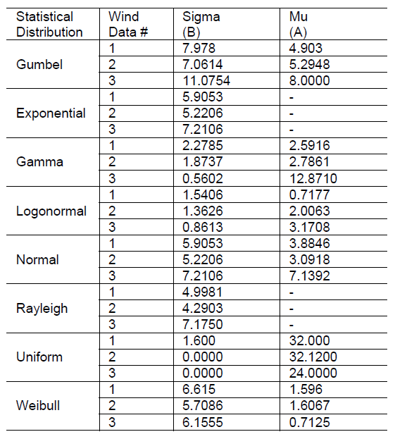
In order to determine the optimal PDLs, we need to estimate the shape and scale parameter of the curves. Using extracted wind data CDFs, we generate the corresponding PDs. According to the obtained PDs, using the graphical method in conjunction with additional ones, all parameters of possible PDLs are determined, to which the studied wind time series may belong. An example is shown in Fig. 3 for the first data array (a). All parameters of possible distributions are given in Table 3.
Fig.3. A graphical wind data analysis
Fig. 3 shows eight PDFs, namely the Gumbel, Exponential, Gamma, Logonormal, Normal, Rayleigh, Uniform, and Weibull, fitted to the wind speed values. Graphically it can be observed that Logonormal PDF gives the best match. The Gamma, Rayleigh and Weibull distributions match the histogram to a lesser degree, and the remaining distributions provide the worst fits.
Similarly, these eight PDFs were also fitted to other two wind series data and it was observed that the Logonormal, Gamma, Weibull, and Rayleigh the best ones for further analyses.
The most widely used distribution of the selected laws is the Weibull distribution. It is easy to use and accurate for most wind conditions that may occur in research. The Rayleigh distribution is a simplified version of the Weibull distribution, characterized by its simplicity due to the use of only one parameter, which negatively affects the quality of the obtained characteristics, and it is not so often suitable. Gamma and lognormal distributions are also two-parameter, they are less common in wind descriptions, but they can be much better suited for a several wind time series [20] (depending on the wind samples specific values repeatability).
Table 3. Wind time series obtained distribution parameters
.
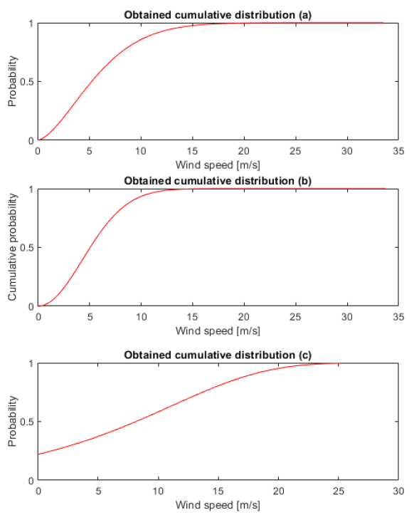
Fig.4. Obtained wind data CDFs
After that, the wind time series is checked using the Pearson’s chi-squared test and Kolmogorov-Smirnov Goodness-of-Fit test according to the laws selected above. For the first sample data, the Weibull distribution meets the goodness-of-fit criteria (Fig. 4a). The second one corresponds to the Rayleigh distribution (Fig. 4b).
For the third sample, the Gambel distribution and the normal distribution were the closest, but neither of them fully satisfied the Kolmogorov test. This may be due to the small number of distribution laws considered, which were proposed in the article, or to the complexity of the original law (multiparameter, multimodal distribution, etc.).
Thus, we can conclude that the tools for finding the probabilistic characteristics of the wind time series presented in this article are extensive, but not always sufficient for the most accurate description of complex laws. For some cases, it may be necessary to use more sophisticated and advanced methods to obtain reliable probabilistic parameters.
Conclusion
The study of the wind speeds CDF was based on real and accurate measurements of these values at three obviously different sites. The results showed that it was possible to fully determine the probabilistic characteristics corresponding to the goodness-of-fit criteria for two of them. Thus, for some investigated wind time series, it will be necessary to expand the initial list of possible CDFs.
The implemented capabilities for modeling the distribution from random variables allow us to model the CDF and PD for the RES active and reactive power of various configurations based on the specific territory wind models.
Acknowledgment – The work was supported by Ministry of Science and Higher Education of Russian Federation, according to the research project № МК-5320.2021.4.
REFERENCES
[1] Zhang, J., M. Cheng, and X. Cai. (2012). Short-Term Wind Speed Prediction Based on Grey System Theory Model in the Region of China. Przeglad Elektrotechniczny, 88 (7a), 67-71. [2] Strzelczyk, F. (2009). Renewable energy sources in power system. Przeglad Elektrotechniczny, 85 (9), 340-349. [3] Karaki, S.H., Chedid, R.B., Ramadan R. (1999). Probabilistic performance assessment of autonomous solar–wind energy conversion systems, IEEE Trans Energy Conversion, 14 (3), 766–772. [4] Kruangpradit P., Tayati W. (1996). Hybrid renewable energy system development in Thailand, Renewable Energy, 8 (1–4), 514–517. [5] Sohoni, V., Gupta, Sh., Nema, R. (2016). A comparative analysis of wind speed probability distributions for wind power assessment of four sites. Turkish Journal of Electrical Engineering & Computer Sciences, 24, 4724-4735. [6] Giraldo, J., Castrillon, J., Granada-Echeverri, M. (2014). Stochastic AC Optimal Power Flow Considering the Probabilistic Behavior of the Wind, Loads and Line Parameters. Ingeniería e Investigación, 15, 529-538 [7] Soroudi, A., Aien M., Ehsan, M. (2012). A Probabilistic Modeling of Photo Voltaic Modules and Wind Power Generation Impact on Distribution Networks. IEEE Systems Journal, 6 (2), 254-259. [8] Malska, W. and D. Mazur. (2017). Analysis of the Impact of Wind Speed for Power Generation on the Example of Wind Farm. Przeglad Elektrotechniczny, 93 (4), 54-57. [9] Akyuz, H., Gamgam, H. (2017). Statistical Analysis of Wind Speed Data with Weibull, Lognormal and Gamma Distributions. Cumhuriyet Science Journal, 38, 68-76. [10] Ross, R. (1994). Graphical Methods for Plotting and Evaluating Weibull Distributed Data. Proceedings of the 4th Int. Conf. Properties and Applications of Dielectric Materials,1, 250 – 253. [11] Cousineau, D., Brown, S., Heathcote, A. (2004). Fitting distributions using maximum likelihood: Methods and packages, Behavior Research Methods, Instruments, & Computers,36, 742–756. [12] Prem, Ch., Siraj, A., Vilas, W. (2018). Study of different parameters estimation methods of Weibull distribution to determine wind power density using ground based Doppler SODAR instrument. Alexandria Engineering Journal, 57 (4), 2299-2311. [13] Dongbum, K., Kyungnam, K., Jongchul H. (2018). Comparative Study of Different Methods for Estimating Weibull Parameters: A Case Study on Jeju Island, South Korea. Energies, 11 (2), 1-19. [14] Seyit, A., Akdağ, A., D. (2009). A new method to estimate Weibull parameters for wind energy applications. Energy Conversion and Management, 50 (7), 1761-1766. [15] Çelik, H., Yilmaz, V. (2008). A Statistical Approach to Estimate the Wind Speed Distribution: The Case of Gelibolu Region. Doğuş Üniversitesi Dergisi, 9 (1), 122-132. [16] Bielecki, S. (2017). Reactive Power Demand – Verification of a Hypothesis of Normal Distribution Values). Przeglad Elektrotechniczny, 93 (9), 20-23. [17] Loic, Q., Clement, J., Christian. E. (2014). Measuring the Power Curve of a Small-scale Wind Turbine: A Practical Example. Conference Proceedings Paper – Energies “Whither Energy Conversion? Present Trends, Current Problems and Realistic Future Solutions”, pp. 1-11. [18] González-Aparicio, I., Monforti, F., Volker, P., Zucker, A., Careri, F., Huld, T., Badger, J. (2017). Simulating European Wind Power Generation Applying Statistical Downscaling to Reanalysis Data. Applied Energy, 199, 155-168. [19] Rosas, P. A. C., Nielsen, A. H., Bindner, H. W., Sørensen, P. E., Lindahl, S. O. R., Nielsen, J. E. & Pedersen, J. K. (2004). Dynamic Influences of Wind Power on The Power System, Technical University of Denmark, Denmark, Forskningscenter Risoe. [20] Lingfeng, W., Chanan, S., Andrew, K. (2010). Wind Power Systems: Applications of Computational Intelligence, Springer-Verlag Berlin Heidelberg.
Authors: Assistant of Division for Power and Electrical ngineering, Yuly Bay, Tomsk Polytechnic University, 30, Lenin Avenue, Tomsk, Russia, E-mail: nodius@tpu.ru; Associate professor of Division for Power and Electrical Engineering, Nikolay Ruban, Tomsk Polytechnic University, 30, Lenin Avenue, Tomsk, Russia, E-mail: rubanny@tpu.ru; Associate professor of Division for Power and Electrical Engineering, Mikhail Andreev, Tomsk Polytechnic University, 30, Lenin Avenue, Tomsk, Russia, E-mail: andreevmv@tpu.ru; Professor of Division for Power and Electrical Engineering, Aleksandr Gusev, Tomsk Polytechnic University, 30, Lenin Avenue, Tomsk, Russia, E-mail: gusev_as@tpu.ru.
Source & Publisher Item Identifier: PRZEGLĄD ELEKTROTECHNICZNY, ISSN 0033-2097, R. 97 NR 12/2021. doi:10.15199/48.2021.12.14
Published by Ameur Fethi AIMER1, Ahmed Hamida BOUDINAR2, Mohamed Amine KHODJA2, Azeddine BENDIABDELLAH2, University of Saida. Algeria (1), University of Sciences and Technology of Oran. Algeria (2) ORCID: 1. 0000-0003-4933-109X
Abstract. Induction machines are enjoying growing interest mainly due to their robustness, their weight to power ratio and their manufacturing cost. However, several faults affect the reliability of these machines. In order to identify these defects, the power spectral density, based on the Periodogram technique is used for its simplicity and its short computing time. However, it is limited in frequency resolution in cases of low motor slip (harmonic close to the fundamental), in the case of very noisy signals (false alarms) and in the detection of incipient faults (low amplitude harmonics) which makes the diagnosis inefficient. To improve the frequency resolution of the spectral analysis, we highlight in this paper the impact of the choice of the weighting windows in order to have a reliable diagnosis of induction motor’s rotor faults. The experimental results will then show the properties of each window to improve the frequency resolution and thus correct the Periodogram’s limits.
Streszczenie. Maszyny indukcyjne cieszą się coraz większym zainteresowaniem głównie ze względu na ich solidność, stosunek masy do mocy oraz koszt wykonania. Jednak kilka usterek wpływa na niezawodność tych maszyn. W celu identyfikacji tych defektów wykorzystuje się gęstość widmową mocy, opartą na technice Periodogram, ze względu na jej prostotę i krótki czas obliczeń. Jest jednak ograniczona w rozdzielczości częstotliwości w przypadkach niskiego poślizgu silnika (harmoniczna zbliżona do podstawowej), w przypadku bardzo zaszumionych sygnałów (fałszywe alarmy) oraz w wykrywaniu początkowych usterek (harmoniczne o niskiej amplitudzie), co sprawia, że diagnoza jest nieskuteczna . Aby poprawić rozdzielczość częstotliwościową analizy spektralnej, w niniejszym artykule zwracamy uwagę na wpływ doboru okien ważenia na wiarygodną diagnozę uszkodzeń wirnika silnika indukcyjnego. Wyniki eksperymentalne pokażą następnie właściwości każdego okna, aby poprawić rozdzielczość częstotliwości, a tym samym skorygować granice Periodogramu. (Poprawa rozdzielczości częstotliwości w diagnostyce usterek silnika indukcyjnego: walidacja eksperymentalna)
Keywords: Induction motor; Fault diagnosis; Broken rotor bars; Frequency resolution. Słowa kluczowe: silnik indukcyjny, diagnostyka, uszkodzenie prętów
Introduction
Nowadays, induction motor is widely used in most electric drives applications, especially at constant speed. Advances in power electronics associated with modern control techniques have led to the consideration of variable speed applications, which were previously limited exclusively to DC motors and synchronous motors. Thus, faced with this growing interest, a general reflection is naturally directed towards the detection of faults and the monitoring of induction machines state. There are several techniques in fault diagnosis; vibration analysis being the most widely used method [1], [2], [3]. This method is mainly used for the detection of mechanical faults.
Motor current signature analysis or MCSA has been used more and more in recent years. Its peculiarity is that the stator current spectrum carries information on almost all of the electrical and mechanical faults that can affect the induction motor [4], [5], [6]. Spectral analysis based on signal processing has been used in recent years in the diagnosis and monitoring of induction machines faults [7]. This technique is well suited to the fault diagnosis insofar as many phenomena result in the appearance of sideband frequencies directly related to the speed of rotation of the motor.
Based on the calculation of the Fourier transform (FT), the power spectral density (PSD) is a widely used tool in research and industry associated with the analysis of stator current [8]. This is justified by the simplicity and the low cost of the current sensors and the harmonic content of the stator current. However, this technique has several drawbacks linked to the problem of frequency resolution. Indeed, the calculation of FT introduces a smoothing effect as well as a negative effect. These effects result in the appearance of sideband lobes in the stator current spectrum [9] and therefore reduce the clarity of the analysis.
When analyzing a signal, it is interested to have a main lobe as narrow as possible and side lobe amplitudes as low as possible, both advantages are impossible to achieve simultaneously. Because of this resolution problem, the PSD find difficulties in detecting faults when harmonic are near to the fundamental (in the case of a low motor slip), of false alarms (in the case of highly noisy signals) and for harmonics of low amplitude (case of incipient faults detection ).
Within this objective, this paper focuses on the choice criteria through experimental tests of the window weights and the impacts of this choice on the detection and localization of induction motor’s rotor faults.
Stator current analysis
The spectral analysis of the stator current knows a growing interest these last years, because of the quantity of information contained in its spectrum on most of the faults which can appear on an induction machine. It is interesting to note that, as in the case of the vibratory analysis, the spectral components of the fault continue to increase with time by the increase of the fault severity [6]. The broken rotor bars faults of the induction motor are considered among the most commonly studied faults because of their simplicity of implementation. This fault induces changes in the spectral components of the stator current and thus generates the appearance of new sideband frequencies in the current spectrum relating to the broken rotor bars fault [7].
Indeed, broken rotor bars give rise to a sequence of sidebands frequencies given by:
.
where: fs is the supply frequency and fc the sideband frequencies associated with the broken rotor bars fault, s is the motor slip and k = 1, 2, 3…
When analyzing the stator current, it is just possible to evaluate the general condition of the rotor. If there are broken rotor bars in various parts of the rotor, the current analysis is not able to provide information on the configuration of non-contiguous broken bars. For example, the frequency component does not exist if broken bars are electrically π/2 radians away from each other.
It should be noted that some experimental studies have demonstrated that both the skewing and non-insulation of rotor bars lead to a reduction of broken rotor bars harmonic components.
Power Spectral Density Calculation
Fourier Transform
The Fourier transform (FT) is a powerful mathematical tool used to extract useful information from a signal in the frequency domain. It is a nonparametric method, which lends itself well to the analysis of stationary phenomena. The FT is given by the following relation [9-10]:
.
where FTx(f) is called the Fourier Transform of the signal x(t), represented in our case by the stator current signal of the induction motor. Of course, it is impossible to analyze the signal over an infinite period. It is therefore necessary to truncate the signal prior to digital processing.
Truncation operation
The signal to be processed must be limited in time, this is said to be truncated. Mathematically, this amounts to do the following operation:
.
where: x(t): is the measured signal; xT(t): is the signal to be processed; ΠT: is the rectangular window; T: is the time length of the window.
However, this truncation operation introduces negative effects on the signal spectrum. Indeed, these effects also known as side lobes appear during this operation. These side lobes result from the brutal impact of truncation of the signal that comes to replace it by zero outside the support of the rectangular window ΠT. These effects reduce the analysis accuracy.
Weighting windows
To resolve the truncation operation effects, we use the weighting windows ωT(t). This implies that the weighted signal xp(t) is processed instead the truncated signal xT(t).
The new signal is given by :
.
While performing a fault diagnosis operation based on peaks detection, it is more suitable to have a main lobe as narrow as possible and side lobe amplitudes very low to avoid false alarms. Unfortunately, it is almost impossible to have both properties in the same time. Thus, the weighting windows are chosen based on the nature of the processed where: signal and the searched compromise.
Table 1. Weighting windows description
.
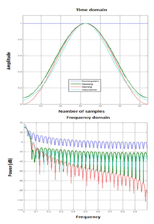
Table 1 gives the main weighting windows used with a compact support. Therefore, we consider the main lobe width at -3dB defined by the parameter L for the frequency resolution Δf, and the amplitude of the highest side lobe given by the parameter A. These windows are shown in Fig. 1 [11].
Fig.1. Representation of the weighting windows
Discrete Fourier Transform
To determine the Fourier transform of a signal using a digital computer, the number of frequencies obtained is limited due to the limited computing power of the computer. It is therefore necessary to substitute the continuous variable f by a discrete variable.
The operation dedicated to the frequency discretization is based on the replacement of the continuous frequency f by the discrete frequency kΔf (where k is an integer). The obtained frequencies are known as frequencies components of the DFT (Discrete Fourier Transform). Since the FT of a digital signal should be periodic with Fe period, the frequency resolution is given for N samples by the following equation:
.
where: Δf : Frequency resolution; ; Fe : Sampling frequency; N : Number of samples (with which we calculate the DFT).
The frequency discretization is than defined by a sampling operation in the spectral domain. Numerically, the DFT is expressed by:
.
FFT Algorithm
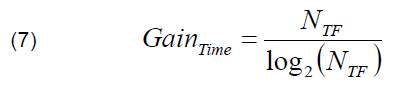
The Fast Fourier Transform, also known as FFT is an algorithm based on fast calculation of the DFT proposed by J.W. Colley and J.W. Tuckey in 1965. The FFT algorithm uses a number of points NTF equal to a power of 2, which results in a computing time gain compared to a classic calculation using the DFT, this gain in time is given by the following equation [11]:
.
If the number of points obtained after the acquisition step is not a power of 2, the record length of the signal is completed with zeros in order to use the FFT algorithm; this procedure is called as the zero padding procedure or the zeros extension step.
Power spectrum
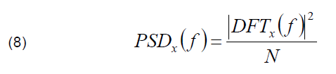
Finally, we define the power spectral density (PSD) as the square modulus of the Fourier Transform. The PSD is independent of the signal phase. In addition, it is always real and positive; it is given by [12]:
.
Experimental tests
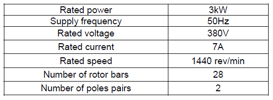
The experimental tests presented in this paper are carried out by the DIAGNOSIS group at the LDEE laboratory at the University of Sciences and Technology of Oran, Algeria. The motor used in these practical tests is a three-phase squirrel cage induction motor coupled to a Direct Current generator used as a load. The parameters of the induction motor are given in the appendix.
In this paper, we deal with the broken rotor bar diagnosis issue; this fault is created artificially in our tests. The measurement chain includes three hall-effect current sensors, an anti-aliasing filter, a tachometer and an acquisition card. Finally, a computer is used to process the acquired signals. this test bench is shown in Fig. 2.
The motor operating modes used to validate the diagnosis procedure are:
– Healthy engine operation. – Motor operating with 01 broken bar at a motor slip of 4.06%. – Motor operating with 01 broken bar at a motor slip of 2.13%
Fig.2. Experimental setup description
Interpretation and discussion
Figure 3 shows the estimation of the power spectral density PSD using the periodogram in the case of 1 broken rotor bar. For this purpose, the spectral analysis is carried out using the four weighting windows studied in this paper. According to eq. (1), the rotor bars fault is located on both side of the fundamental at a particular frequency. For this test, the motor slip is 4.06% which gives a sideband frequency signatures around 45.94Hz and 54.06Hz for k=1. This frequency signature is repeated for the values of k=2,3…etc. Indeed, the parameter k represents the multiplicity of the fault frequency signatures on the spectrum.
Fig.3. Stator current PSD with various weighting windows for 1 broken rotor bar and a motor slip of 4.06 %
Fig.4. Stator current PSD with various weighting windows for 1 broken rotor bar and a motor slip of 2.13 %
For the rectangular window, the frequencies are barely detectable. Whereas for the other windows, the detection of these frequencies is easier. It should be noted that the Hanning window is distinguished by a larger main lobe compared to the Hamming and Gaussian windows. On the other hand, this same Hanning window gives the sideband frequencies with the greatest amplitude.
For the last test shown in Fig. 4, the power spectral density PSD per Periodogram of the stator current in the case of 1 broken rotor bar is highlighted. In this test, the motor slip is equal to 2.13% which gives sideband frequencies close to the fundamental. These frequencies calculated using eq. (1) are located around 47.87Hz and 52.13 from either side of the fundamental. For this low value of the motor slip, the sideband frequencies of the broken rotor fault are too close to the fundamental.
Under these conditions, localization using the rectangular window is almost impossible due to the position of the sideband frequencies regarding the fundamental. For the Hamming and Gaussian windows, the localization is difficult and less obvious compared to the Hanning window. Indeed, the Hamming and Gaussian windows offer a narrow main lobe and therefore are best suited for cases of low motor slip.
Finally, the Hanning window is more suitable in the case of incipient faults, given the large amplitude of the side lobes.
Conclusion
This paper investigates the influence of the weighting windows choice on the frequency resolution of the stator current spectrum. In this aim, we present three weighting windows used to resolve the resolution problems due to the rectangular window use. Indeed, a proper choice of the weighting window is necessary to study critical cases that may arise (e.g. case of low motor slip and incipient faults).
To assess each window, we take into consideration the study of fault diagnosis of broken rotor bars and its identification using the power spectral density spectrum. Through the study of each window, we searched a compromise between a narrow main lobe width and side lobes amplitude. This compromise was clearly shown by the experimental results presented in this paper. It has been observed that the Hanning window gave side lobes of low amplitude but the main lobe is wider.
Furthermore, windows Gaussian and Hamming offer the possibility of having a narrow main lobe but the side lobes has more amplitude than that obtained with the Hanning.
Finally, we can say that the Hanning window is recommended for the diagnosis of incipient faults and the Hamming window or Gaussian window is more appropriate in the case of faults too close to the fundamental. The next step will be devoted to the development of an adaptive process composed of several weighting windows. This process will be achieved using Artificial Intelligence.
Appendix. Induction motor parameters
.
REFERENCES
[1] H. Henao, G.A. Capolino, M.F. Cabanas, F.Fiippetti, C. Bruzzese, E. Strangas, R. Pusca, J. Estima, M. Riera-Guasp, S.H. Kia, Trends in fault diagnosis for electric machines: A review of diagnostic methods. IEEE Industrial Electronics Magazines, June 2014 [2] W. Li, C.K. Meshefske, Detection of induction motor faults: a comparison of stator current, vibration and acoustic methods, Journal of Vibration and Control, vol. 12, pp. 165-188. 2006 [3] B. Liang, S.D. Iwnicki, A.D. Ball, Asymmetrical stator and rotor faulty detection using vibration, phase current and transient speed analysis, Mechanical Systems and Signal Processing, Elsevier, vol. 17, pp. 857-869. 2003 [4] A.F. Aïmer, A.H. Boudinar, N. Benouzza, A. Bendiabdellah, Simulation and Experimental Study of Induction Motor Broken Rotor Bars Fault Diagnosis using Stator Current Spectrogram, In Proc. of IEEE 3rd International Conference on Control, Engineering & Information Technology (CEIT), Tlemcen, Algeria. 25-27 May 2015. [5] A. H. Bonnett and C. Yung, Increased Efficiency Versus Increased Reliability, Industry Applications Magazine, IEEE, vol. 14, pp. 29-36, 2008 [6] M. M. Rahman, M. N. Uddin, Online Unbalanced Rotor Fault Detection of an IM Drive Based on Both Time and Frequency Domain Analyses, IEEE Transactions on Industry Applications, vol. 53, no. 4, pp. 4087-4096, July-Aug. 2017 [7] M.E.H. Benbouzid, M. Viera, C. Theys, Induction motors’ faults detection and localization using stator current advanced signal processing techniques, IEEE Trans. on Power Electronics, vol. 14, pp. 14-22, January 1999 [8] M.E.H. Benbouzid, A review of induction motors signature analysis as a medium for faults detection, IEEE Trans. on Industry Electronics, vol. 47, pp. 984-993, October 2000 [9] F. Filippetti, A. Bellini and G. A. Capolino, Condition monitoring and diagnosis of rotor faults in induction machines: State of art and future perspectives, IEEE Workshop on Electrical Machines Design Control and Diagnosis (WEMDCD), Paris, 2013 [10] A. Bendiabdellah, A.H. Boudinar, N. Benouzza, M. Khodja, The enhancements of broken bar fault detection in induction motors. In Proc. of Intl Aegean Conference on Electrical Machines & Power Electronics (ACEMP), Intl Conference on Optimization of Electrical & Electronic Equipment (OPTIM) & Intl Symposium on Advanced Electromechanical Motion Systems (ELECTROMOTION), Side, Turkey, 02-04 Sep. 2015 [11] A.F. Aimer, A.H. Boudinar, M.A. Khodja, A. Bendiabdellah, Assessment of windowing effect on the frequency resolution of the stator current PSD for induction motor broken rotor bars diagnosis, IEEE 1st International Conference on Innovative Research in Applied Science, Engineering and Technology IRASET, Meknes, Marocco 16-19 Apr. 2020 [12] M.B. Koura, A.h.Boudinar, A. Bendiabdellah, A.F. Aimer, Z. Gherabi, Rotor faults diagnosis by adjustable window, Przeglad Elektrotechniczny Journal. March 2021. Vol. 97, Issue 3. pp.123-129
Authors: Dr. Ameur Fethi AIMER, Diagnosis Group-LDEE Laboratory. University of Saida, Algeria. Email: fethi.aimer@yahoo.fr Prof. Ahmed Hamida BOUDINAR, Diagnosis Group-LDEE Laboratory. USTO-Oran, Algeria. Dr. Mohamed Amine KHODJA, Diagnosis Group-LDEE Laboratory. USTO-Oran, Algeria. Prof. Azeddine BENDIABDELLAH, Diagnosis Group-LDEE Laboratory. USTO-Oran, Algeria.
Source & Publisher Item Identifier: PRZEGLĄD ELEKTROTECHNICZNY, ISSN 0033-2097, R. 97 NR 11/2021. doi:10.15199/48.2021.11.12
Published by Stanislav S. GIRSHIN, Oleg V. KROPOTIN, Vladislav M. TROTSENKO, Aleksandr O. SHEPELEV, Elena V. PETROVA, Vladimir N. GORYUNOV, Omsk State Technical University, Omsk, Russia
Abstract. The use of a simplified formula for calculation of active power losses in transmission lines taking into account the temperature in the stationary thermal regime is considered. The results of the comparison of losses calculated using a simplified formula and based on the solution of the full heat balance equation for wires of various types are presented. The dependences of the calculating errors on the load current with and without solar radiation are constructed and analyzed.
Streszczeni. W artykule rozważa się korzystanie z uproszczonej formuły do obliczania strat mocy czynnej w linii z uwzględnieniem temperatury w trybie stacjonarnym cieplnym. Straty oblicza się według uproszczonego wzoru i w oparciu o równania bilansu cieplnego dla przewodów różnych typów. Zbudowane są i analizowane zależności błędów obliczeń od prądu obciążenia z promieniowania słonecznego i bez niego. Uproszczone zależności do obliczania strat mocy czynnej w linii z uwzględnieniem temperatury
Keywords: bare and insulated wires, energy losses, temperature. Słowa kluczowe: gołe i izolowane przewody, straty energii, temperatura.
Introduction
Load losses of energy in power lines account for about 85% of the total losses in the lines and about 55% of the total losses in the electrical networks of Russia. Improving the efficiency of power transmission imposes rather high demands on the accuracy of the calculation of losses. This in turn leads to the necessity of taking into account all the main factors determining the amount of losses. One of these factors is the temperature dependence of active resistance [1-3].
The papers in the field of accounting for the temperature of wires in the calculation of energy losses in electrical networks are rather popular nowadays [4-8]. However, the relevant methods are not widespread, in addition to the standards presented in [9-10]. For example, modern programs for calculating energy losses usually take into account only the dependence of active resistances on the ambient temperature, but not heating by current. The main reason for this is that a fairly large amount of additional input data is required to accurately calculate the temperature.
The problem can be formulated as follows: it is required to develop such methods for calculating energy losses, which would take into account both the ambient temperature and the heating of the wires by the load currents, but would require a minimum amount of source data.
In this article, a simplified formula for heat loss is compared with more complex methods.
Basic equations and formulas
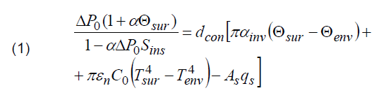
In the established thermal mode, the surface temperature of the insulated wire Θsur can be calculated by the equation of heat balance per unit length of the line [5]:
.
where ΔP0 = I2r0 is active power losses in the wire with linear resistance r0. reduced to 0 ºC [kW/km]; I is current [A]; α is temperature coefficient of resistance [ºC-1]; Θsur and Θenv is the surface temperature of the wire and the environment temperature [ºC]; dcon is wire diameter [m]; Sins is linear thermal insulation resistance [(ºC·m)/W]; αinv is heat transfer coefficient by forced convection [W/(m2·К)]; εп is wire surface blackness ratio for infrared radiation; C0 = 5,67·10-8 [W/(m2·K4)] is black body radiation constant; Tsur and Tenv are absolute temperatures of the surface of the wire and the environment [K]; As is absorption capacity of the wire surface of solar radiation; qs is solar radiation flux density on the wire [W/m2].
Equation (1) is written under the assumption that the temperature gradient in the conductor is zero. Then the temperature of the conductor wire is related to the temperature of its surface by a simple ratio:
.
where ΔP is active power losses, which is the left (and right) part of equation (1).
In equation (1), the losses in the left part are written as a function of the surface temperature of the wire (in order to eliminate the temperature of the core). It is easy to show that the relation:
.
is equivalent to a formula:
.
Bare wire can be considered as a special case when Sins = 0. In the absence of isolation, the heat balance equation takes the form [5]:
.
The above formulas allow us to determine the temperature of the wire and the losses of active power taking into account the heating. The main drawback of this approach is that a large number of additional source data is needed: the parameters Θenv, Sins, αinv, εп, As, qs. The greatest problem is the heat transfer coefficient and solar radiation, which are determined by the whole set of meteorological conditions and vary not only in time but also along the route of each line (in particular, αinv and qs depend on the azimuth of the wire axis).
The main idea of the simplification of the task is the linearization of equations (1) and (5) as follows:
.
where R0 is active resistance of the wire at 0 ºC [Ω]; A is the constant coefficient which determines the intensity of heat transfer from the wire to the environment.
Equation (6) is considered fair for both bare and insulated wires. Calculation per phase and per unit length in this case does not make sense anymore, therefore equation (6) is written for the three-phase line, and the resistance R0 is reduced to the actual length. Thus, the left side of equation (6) represents the power loss in the entire line.
Having resolved (6) with respect to the temperature of the wire and substituting the result in the left side of the equation, we obtain the final formula for the losses in the line taking into account heating:
.
The numerator in this expression is the losses reduced to the environment temperature, and the denominator takes into account the increase in losses due to heating of the wires with a load current.
The coefficient A is determined by equation (6) at the maximum allowable current Iall:
.
where Θall is maximum wire temperature [ºC]; Θenv1 is the temperature of the environment to which the maximum allowable current is reduced [ºC].
It can be seen that formulas (7) and (8) require a much smaller amount of source data compared to equations (1) and (5). Only the ambient temperature is required out of the entire set of meteorological parameters.
Comparative analysis
The results of comparison of the temperature of the wire and the power losses in the line, calculated by the simplified equations (6)-(8) and by the full models (1), (2), (5) are given below. The following objects were chosen as comparison objects:
bare wires of standard construction AS-240/32; high voltage insulated wires SIP-3 1×95 (analogue SAX); high temperature bare wires ACCR-405-T16.
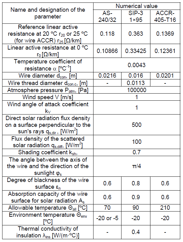
In all cases, a three-phase wiring system is considered. The parameters of the wires and cooling conditions are presented in Table 1.
The heat transfer coefficient, thermal insulation resistance and the flux density of solar radiation were determined by the following formulas [5], [6]:
.
The maximum value of direct solar radiation at the earth’s surface is about 1000 W/m2. However, this value cannot be used to calculate energy losses, since direct solar radiation has an annual and daily rate, decreasing to zero at night. Therefore, the averaged value was used in the calculations, for which, in the first approximation, half the maximum was taken, that is qs,dir = 500 W/m2.
Table 1. Source data for calculations
.
Scattered radiation also has an annual and daily rate. The data allow to accept as a typical value qs,diff = 100 W/m2.
The shading coefficient ksh shows how much of the total line length is, on average, illuminated by the sun during daytime hours. The value of ksh = 0.7 is chosen taking into account the fact that the main part of the existing lines passes at sufficiently large distances from high structures. For lines of 110 kV and above, we should expect even higher values of the shading coefficient, since the supports have a greater height, and the main part of the lines passes in uninhabited areas. However, for 10 kV lines located near communications, the shadow coefficient may, on the contrary, be lower.
The angle between the axis of the wire and the direction of sunlight φs is assumed to be 45º as the average value between zero and 90º. In reality, it is determined by the average azimuth of the wire and the latitude of the terrain.
Tables 2-5 and Fig. 1-5 show the results of loss and temperature comparison for the wires under study. Tables 2-4 are built under the following conditions:
• environment temperature is minus 20 ºC; • allowable currents are calculated on the basis of equations (1), (2) or (5) with the data presented in Table 1, but excluding solar radiation.
The low air temperature is chosen due to the fact that this corresponds to the expansion of the operating temperature range of the wires. As a result, the differences between exact and simplified methods become more pronounced.
The data in Table 5 were obtained with the reference value of the allowable current, taking into account the correction factor for the ambient temperature. The temperature of the environment is at a minimum level of -5 ºC, included in the table of correction factors.
Table 2. The results of the comparison of power losses and temperature of the wires AS-240/32 with the calculated allowable current
.
Table 3. The results of the comparison of power losses and temperature of the wires SIP-3 1 × 95 at the calculated allowable current
.
Table 4. The results of the comparison of power losses and temperature of the wires ACCR-405-T16 at the calculated allowable current
.
Table 5. The results of the comparison of power losses and temperature of the wires AS-240/32 at reference allowable current
.
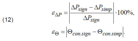
The load current I is expressed in fractions of the allowable current. The subscript “sign” for temperature and active power losses indicates the exact value calculated by equations (1), (2) and (5). The subscript “simp” corresponds to the simplified formulas (6) – (8). For the external temperature of the insulated wire, the additional index is not indicated, since the external temperature can only be calculated from the full model. Each Table also shows the relative errors in calculating the power losses εΔP using the simplified formulas compared with the full formula (1), (2) or (5), and the absolute errors in calculating the temperature of the wire εΘ using the same methods:
.
Fig.1. Dependences of active power losses on the load current for the AS-240/32 wires at the calculated allowable current without solar radiation
Fig.2. Dependences of active power losses on the load current for the ACCR-405-T16 wires at the calculated allowable current with solar radiation
Fig.3. Dependences of active power losses on the load current for the AS-240/32 wires at the reference allowable current without solar radiation
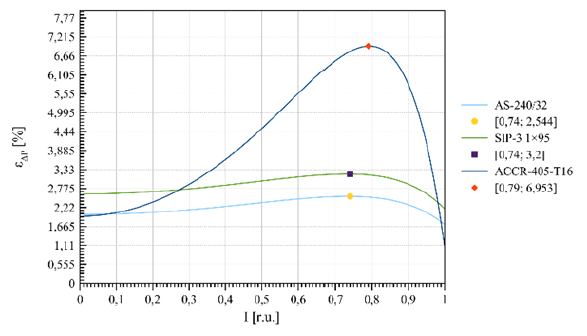
Fig.4. Calculating errors of power losses by simplified formulas at the calculated allowable current without solar radiation
Fig.5. Calculating errors of power losses by simplified formulas at the calculated allowable current with solar radiation
It can be seen that the simplified formula gives the greatest accuracy for the wires AS-240/32 at the calculated allowable current. The dependences of power losses on the load current without solar radiation, constructed according to exact and simplified formulas, are practically the same on the scale of Figure 1. The calculating error for insulated wires slightly increases, but this increase is not significant. From a practical point of view, the error in calculating losses by simplified formulas becomes significant only for ACCR wires, where it can exceed 5%. The dependence of the calculating error on the type of wire is due to the increase in the operating temperature range: for the AS wires, with received data, it is 90 ºC, for SIP – 110 ºC, and for ACCR – 230 ºC.
The error in calculating power losses is conditionally systematic: the simplified method gives lower values of temperature and power losses compared to exact equations. However, a constant component of the error cannot be determined without taking into account solar radiation, since the error becomes zero at the allowable current and at zero.
Solar radiation at the accepted values of its intensity leads to additional heating of wires by 4-7ºC and to an increase in active power loss by about 2% (Tables 2-4). As a result, the difference between the exact and simplified methods increases with the appearance of the constant component of the error.
When using the calculated allowable current, the dependences of the calculating error on the load current have a clearly defined maximum both with and without solar radiation. The maximum points are highlighted in Fig. 4 and 5 with the abscissa and ordinate indicated. For all cases, the peaks are observed roughly in the same area – about 75-80% of the allowable current. At lower currents, the calculating errors are reduced due to the fact that the temperature of the wires decreases and the thermal change in resistance becomes less significant. The decrease in errors with increasing current over 80% of the allowable one is due to the fact that the coefficient A in the simplified formula is chosen from the condition of equality of the losses at the allowable current according to the exact and simplified methods. Therefore, with an allowable current, the error approximately corresponds to the constant component due to solar heating, and without solar radiation, this error is zero.
The considered laws are fully valid only for the case when the allowable current is calculated on the basis of the full heat balance equation. If the reference value of the allowable current is used in the calculations, which is not quite consistent with all the actual cooling conditions, the calculating error increases significantly when the simplified formula is used (Table 5, Fig. 3). Since the reference values of allowable currents are almost always less than the actual ones, the simplified formula in this case, on the contrary, gives overestimated values of the power losses. Corresponding errors may exceed 10%.
Conclusion
The results of the comparison of the accurate and simplified methods for calculating the active power losses in power lines taking into account the temperature allow us to draw the following conclusions:
1. In standard bare AS wires, as well as in insulated SIP-3 wires, the calculating error of losses by the simplified method does not exceed 3.2% compared to exact equations. The calculating error of losses in these wires becomes less than 1% in the absence of solar radiation.
2. Solar radiation increases the losses by about 2% regardless of the load. This should be considered the maximum estimate, since the conditions adopted in the calculations roughly correspond to the maximum possible average annual solar radiation. Consequently, this factor has almost no effect on the effectiveness of the measures to reduce energy losses and, therefore, in almost all cases can be excluded from the calculations.
3. In high-temperature wires, the calculating error may slightly exceed 5%; this is observed in the load range of about 70-90% of the allowable current.
These conclusions are valid for the stationary thermal regime and provided that the allowable current used in the simplified formulas fully corresponds to the exact equation of thermal balance. Reducing the accuracy with which the allowable current is set, leads to a significant increase in the calculating error of the losses (to about 10% in the AS wires).
The developed technique can be used for calculation and reduction of the energy losses in AS and SIP wires, as well as in most cases in wires of increased capacity. It allows taking into account the dependence of the resistance on temperature and at the same time avoiding the cumbersome calculations typical for solving the equations of thermal balance. The simplified formula for power losses has a clear physical meaning and requires only two additional data as compared to calculations without taking temperature into account: the allowable current and the environment temperature.
REFERENCES
[1] D. Douglass, “Weather-dependent versus static thermal line ratings [power overhead lines]”, Power Delivery IEEE Transactions on, vol. 3, no. 2, pp. 742-753, Apr. 1988. [2] V.T. Morgan, “Effect of elevated temoerature operation on the tensile strengthof overhead conductors”, Power Delivery IEEE Transactions on, vol. 11, no. 1, pp. 345-352, Jan. 1996. [3] S.L. Chen, W. Z. Black, H. W. Loard, “High-temperature ampacity model for overhead conductors”, Power Delivery IEEE Transactions on, vol. 17, no. 4, pp. 1136-1141, Oct. 2002. [4] S.S. Girshin, A. A. Bubenchikov, T. V. Bubenchikova, V. N. Goryunov and D. S. Osipov, “Mathematical model of electric energy losses calculating in crosslinked four-wire polyethylene insulated (XLPE) aerial bundled cables,” 2016 ELEKTRO, Strbske Pleso, 2016, pp. 294-298. DOI: 10.1109/ELEKTRO.2016.7512084. [5] H. Kocot, P. Kubek “The analysis of radial temperature gradient in bare stranded conductors,”Przegląd Elektrotechniczny, vol.10, pp. 132–135, 2017. DOI: 10.15199/48.2017.10.31. [6] S.S., Girshin, A.A.Y, Bigun, E.V., Ivanova, E.V., Petrova, V.N., Goryunov, A.O., Shepelev The grid element temperature considering when selecting measures to reduce energy losses on the example of reactive power compensation // Przeglad Elektrotechniczny. 2018. No. 8. P. 101-104. DOI 10.15199/48.2018.08.24. [7] J., Teh, I., Cotton Critical span identification model for dynamic thermal rating system placement // IET Generation, Transmission & Distribution. 2015. Vol. 9, Iss. 16, pp. 2644-2652. DOI: 10.1049/iet-gtd.2015.0601. [8] Goryunov V.N., Girshin S.S., Kuznetsov E.A. [and etc.] A mathematical model of steady-state thermal regime of insulated overhead line conductors // EEEIC 2016 – International Conference on Environment and Electrical Engineering 16. 2016. С. 7555481. [9] “Std 738”, Standard for calculating the current temperature of bare overhead conductors, 2006. [10] “Thermal behaviour of overhead conductors”, Aug. 2002.
Authors: Stanislav S. Girshin, e-mail: stansg@mail.ru: Oleg V. Kropotin, e-mail: kropotin@mail.ru.; Vladislav M. Trotsenko, e-mail: troch_93@mail.ru; Aleksandr O. Shepelev, e-mail: alexshepelev93@gmail.com; Elena V. Petrova, e-mail: kpk@esppedu.ru; Vladimir N. Goryunov, e-mail: vladimirgoryunov2016@yandex.ru. Correspondence author e-mail: alexshepelev93@gmail.com
Source & Publisher Item Identifier: PRZEGLĄD ELEKTROTECHNICZNY, ISSN 0033-2097, R. 95 NR 7/2019. doi:10.15199/48.2019.07.10
Published by Ivan KOSTIUKOV, National Technical University “Kharkiv Polytechnic Institute”, Department of Electrical Insulation and Cable Engineering, Ukraine
Abstract. This paper gives a description of measurement method which can be used in practice of carrying out measurement of stray inductance of tested capacitive object with the unknown value of electrical capacitance. Stray inductance is determined by means of analysis of previously smoothed by the least squares method curves of discharge current caused by overdamped discharge of tested capacitive object. An example of practical implementation and the analysis of factors that affect the accuracy of proposed method are also given.
Streszczenie. W artykule opisano metodę pomiarową, która może być zastosowana w praktyce do pomiaru indukcyjności rozproszonej badanego obiektu pojemnościowego przy nieznanej wartości pojemności. Indukcyjność rozproszoną wyznacza się na podstawie analizy wygładzonych wcześniej metodą najmniejszych kwadratów krzywych prądu wyładowania wywołanego rozładowaniem badanego obiektu pojemnościowego. (Oszacowanie indukcyjności rozproszonej kondensatorów na podstawie analizy prądów rozładowania)
Keywords: correlation coefficient, dielectric permittivity, insulation testing, voltage drop. Słowa kluczowe: indukcyjność roz[proszona, kondensator, prąd rozładowania
Introduction
The value of electrical capacitance is among various other factors that can cause a significant impact on technical performance of high voltage equipment, which is used in electrical engineering. Due to the dependence on the value of relative dielectric permittivity, this characteristic of electrical insulation is quite sensitive to the presence of humidity [1]. Therefore, the values of electrical capacitance and dielectric permittivity can be efficiently used in various practical applications which require the assessment of quality of electrical insulation [2-4]. Besides, the value of electrical capacitance is among other factors that influence the value of power losses in insulation of electrical equipment [5]. In practice the problem of electrical capacitance measurement can be solved by applying various technical solutions. Numerous methods of measurement are based on the applying of AC bridges, for example Schering bridge [6]. Another wide spread approach for electrical capacitance measurement implies the determination of time constant of the discharge process [7]. Some other research, focused on electrical capacitance and impedance measurement, have been concentrated on the development of measurement techniques based on the applying of quasi-balanced circuits [8], schemes with phase detectors [9], measurement schemes which imply the applying of various techniques for digital signal processing [10], applying of impedance–to-voltage converters [11], as well as specialized integrated circuit AD5933 [12].
In majority of cases the analysis of technical performance of measurement schemes is carried out under the assumption of negligible impact of parasitic parameters of tested object on their technical performance. However, in case if it is necessary to carry out the assessment of technical state of electrical insulation which operates in high voltage equipment, the presence of some inevitable stray inductance of tested object often can lead to certain difficulties in physical interpretation of the obtained results. Despite the efforts devoted to solving the problem of stray inductance mitigation, it affects some regimes of operations even for such almost entirely capacitive objects as various types of electrical capacitors [13-15] and capacitive voltage dividers [16]. Mentioned difficulties are caused by the fact that the inevitable stray inductance of tested object in some regimes of measurement can cause the increasing of measured values of electrical capacitance with the increasing of frequency of applied voltage. As the increasing of frequency of applied voltage usually leads to more or less distinct decreasing of relative dielectric permittivity, depending on specific types of polarization valid for a particular dielectric material, such increasing of electrical capacitance complicates physical interpretation of the obtained results of measurement. The increasing of electrical capacitance usually becomes more significant in case when frequency of applied voltage approaches the resonant frequency of tested object, i.e. with the increasing of frequency of applied voltage. Besides mentioned difficulties in physical interpretation of obtained results of electrical capacitance measurements, it is obvious that the presence of stray inductance inevitably causes certain difficulties in the assessment of the dielectric dissipation factor. In case of negligible stray inductance of tested object and parallel equivalent scheme of tested capacitive object with power losses the value of dissipation factor can be determined according to the usual relation:
.
where: ω is the value of angular frequency of applied voltage, Cp, Rp are the values of electrical capacitance of tested object and shunt resistance caused by power losses. As it can be concluded from (1), possible inaccuracy of carried out measurements of Cp, Rpcaused by the presence of stray inductance results in inaccuracy of dissipation factor measurements. Consequently, the presence of some stray inductance of tested capacitive object can distort the results of measurements and causes misconceptions about the technical state of tested object. Therefore, for practical applications it is necessary to develop methods of measurements which can be used in order to carry out the assessment of stray inductance of tested capacitive object.
The problem of stray inductance estimation is actual not only in issues that concern the assessment of quality of electrical insulation, but also for other practical applications of electrical engineering, such as the formation of high values of current pulses with specified requirements to their time dependence. The inductance of the discharge circuit affects time dependence of current pulses [17] and, therefore, this time dependence is also affected by the additional contribution caused by the stray inductance of storage capacitor.
The objective of this paper is the elaboration of method for the estimation of stray inductance of tested capacitive object, based on the analysis of transients in electrical circuits that occur due to the overdamped discharge of tested capacitance.
Illustration of the affect of stray inductance on the accuracy of electrical capacitance measurement
Fig. 1 presents the results of carried out measurements of electrical capacitance of a batch of high voltage pulse capacitors with nominal value of capacitance equal to 140 μF and operating voltage equal to 5 kV. All measurements have been carried out by applying series equivalent scheme of tested capacitor with power losses and by means of using digital DE-5000 RLC meter.
Fig.1. Results of electrical capacitance measurements of a batch of high voltage capacitors for two different frequencies
Fig.2 represents the increment of electrical capacitance caused by the increasing of frequency of applied voltage from 100 Hz to 1000 Hz.
Fig.2. The increasing of electrical capacitance caused by the increasing of frequency of applied voltage from 100 Hz to 1000 Hz
From Fig.2 it can be seen that the increasing of frequency of applied voltage leads to previously mentioned increasing of electrical capacitance, which can be noticed for any of tested high voltage capacitors. It is obvious that for the case of unknown values of stray inductance of tested capacitor, shunt resistance, caused by dielectric power losses, and also for the unknown value of electrical capacitance, which can be affected by the presence of moisture, such increasing of electrical capacitance complicates physical interpretation of obtained results of measurements, as it contradicts the admissible dependence of the relative dielectric permittivity on frequency of applied voltage.
Materials and methods
Elaborated method for the estimation of stray inductance is based on the analysis of discharge current curves for the overdamped discharge regime of tested capacitive object. All discharge processes have been considered for the case of the equivalent scheme of the discharge circuit presented on Fig. 3, which is pretty typical for example in practice of modelling discharge processes in generators of pulse currents with high voltage pulse capacitors.
As it can be seen from Fig. 1, the presence of parasitic parameters of tested object L1 and R1 disenables the direct measurements of voltage on an unknown capacitance.
However, in practice it is possible to measure the value of voltage drop on the outputs of current to voltage converter, represented by resistance R2 on Fig. 2. Assuming negligible inductance of discharge circuit L2, this voltage can be represented as a sum of voltages on the unknown electrical capacitance, stray inductance and resistance, caused by power losses in tested object:
.
where UC1(t), UR1(t) and UL1(t) respectively denote the values of voltage drop on the unknown capacitance, power loss resistance of tested object and stray inductance of tested object.
Fig.3. Equivalent scheme for the discharge circuit: C1 represents the value of unknown electrical capacitance, R1 denotes the value of resistance caused by power losses in tested object, L1 is the value of stray inductance of tested object, L2 is the value of inductance of the discharge circuit, R2 represents electrical resistance which is used in order to adjust the discharge regime and also used as a current-to-voltage converter.
In this case it is necessary to consider two cases that correspond to different ratios between the values of R2 and R1.The first case corresponds to the insignificant resistance caused by power losses in tested object. In this simplest case it is possible to assume that the value of voltage on R2 in each moment of transient is equal to the sum of voltages on capacitance and stray inductance. In this case it is possible to neglect with the value of voltage on R1 and the value of voltage on the output of current-to-voltage converter UCONV1 can be written as:
.
The second case corresponds to the significant value of the internal resistance R1. In this case in is necessary to carry out measurements of R1 and make appropriate processing of obtained oscillograms in order to obtain the array of data which is determined only by the values of voltage drop on stray inductance and measured capacitance. In this case the value of voltage on the output of current-to-voltage converter UCONV2 can be written as:
.
Hence, in both cases processed time dependence of voltage is determined by the value of voltage drop on measured capacitance and stray inductance. In order to carry out measurement of stray inductance it is necessary to distinguish the exact contribution of each of these components to their sum, which is available for measurements.
Separation of component of voltage drop on stray inductance of tested object from the component of voltage drop on the unknown capacitance can be carried out by considering the relation which determines correlational relationships between signals.
.
where ρ denotes the value of correlation coefficient, uC(t) and uL(t) respectively denote time dependencies of voltage on measured capacitance and stray inductance. The upper boundary of integration b corresponds to the instant of transient termination, while the lower boundary of integration a1 varies in a range of values that correspond to time interval from the beginning of transient to the value of Tc, which can be determined according to:
.
where h denotes time duration between two samples of analyzed signal, n is arbitrarily selected integer number.
Subsequent analysis and calculations according to (5) will be carried out by using the following relations (7-9) for the discharge current [18]:
.
where U0 is the initial value of voltage on measured capacitance and α1, α2 can be determined by using the following relations: where U0 is the initial value of voltage on measured capacitance and α1, α2 can be determined by using the following relations:
.
where L is the total inductance of the discharge circuit, R is total value of resistance of the discharge circuit that includes both values of R1 and R2:
.
Further analysis also will be carried out for the case when the parameters of the discharge circuit satisfy the relation which allows to consider that |α1| << |α2|. Fig. 4 presents the results of carried out according to (5) calculations. All calculations have been carried out for the value of C1equal to 4.7·10-6 F and L1 + L2 equal to 15·10-2 H.
Fig.4. Correlation coefficient determined for variable lower boundary of integration
As it can be seen from Fig. 4, the increasing of lower boundary of integration leads to the increasing of ρ, which reaches 1 and stays invariable for higher values of a1. Such tendency becomes more distinct with the increasing of resistance of the discharge circuit. For the region with ρ equal to 1 it is rather difficult to distinguish the exact contribution of voltage drop on stray inductance and capacitance to their sum, which is available for measurements. However, for the value of ρ equal to 0 such separation can be carried out by using the orthogonality of analyzed signals. In order to carry out such separation of components of voltage drop, (4) should be written in the following form:
.
The value of stray inductance, similalry to the values of voltage drop on these elements of equivalent scheme on Fig. 3, can be determined by means of multiplying (11) on time derivative taken from time dependence of the discharge current and by making integration from previously determined according to (5) value of the lower boundary of integration a1, which corresponds to zero value of (5), to the value of b, which corresponds to the moment of transient termination. In this case it can be noticed that due to the absence of correlation between the corresponding time dependencies of voltage drop the second term in the right side of (11) is equal to 0. Consequently, in this case (11) can be reduced to the following relation:
.
By taking into consideration (12), the value of stray inductance can be determined as:
.
As the absence of correlation between time dependencies of voltage drop on stray inductance and measured capacitance is essential for making calculations according to (13), comprehensive description of proposed method should include the analysis of conditions for which the value of calculated according to (5) correlation coefficient is equal to zero. The upper boundary of integration b in (5) corresponds to the moment of transient termination and, therefore, antiderivative function for the numerator of (5) is equal to zero for the moment of time b. Consequently, it is sufficient to carry out such analysis only for time dependence of antiderivative function in the numerator of (5). This antiderivative function can be written in the following form:
.
where D(t) can be determined by the following relation:
.
It is necessary to emphasize that all the results of calculations presented on Fig. 4 have been carried out for the values of voltage drop on electrical capacitance (uC(t)) and stray inductance (uL(t)) of tested object. However, due to the presence of parasitic parameters L1 and R1 of capacitive object the exact value of voltage on capacitance which is used in (5) is unavailable for direct measurements. The same problem is valid for the value of voltage drop on stray inductance. Therefore, both time dependencies of voltage drop, which are necessary for carrying out calculations according to (5), are unavailable for direct measurements. Nevertheless, it can be shown that for practical calculations it is sufficient to carry out the assessment of lower boundary of integration a1, that corresponds to zero value of (5), without taking into consideration the exact values of voltage drop on stray inductance and by processing only experimentally obtained curves of the discharge current. As time dependence of the discharge current is available for direct measurements, the determination of the lower boundary of integration a1 can be carried out by the analysis of antiderivative, determined for the result of multiplication of time derivative for the discharge current and antiderivative for the discharge current. This antiderivative function can be determined according to (16):
.
As it can be noticed, (15) and (16) have different denominators. Nevertheless, mentioned difference does not affect the accuracy of a1 determination, as for both cases of F1(t) and F2(t) the value of a1 will be obtained as a root of the following relation:
.
Consequently, instead of determination of a1 by applying the root of determined according to (14) function F1(t), which implies the applying of values of voltage on stray inductance and capacitance which are unavailable for direct measurements, the value of a1 can be efficiently determined by finding the root of F2(t).
Calculation of stray inductance according to (13) requires the determination of time derivative for the discharge current. Therefore, it should be taken into consideration that in case of processing of digital signals by means of various numeric methods, for example by the finite differences method, even small perturbations in sampled signal will result in a pretty significant perturbations in calculated time derivative. Therefore, in practice it is preferable to process previously smoothed curves by applying the least squares method with the help of the following relation:
.
where A, B, C, D are coefficients, determined by means of applying the least squares method. Therefore, for smoothed by the least squares waveform of the discharge current previously mentioned antiderivative determined for the result of multiplication of time derivative for the discharge current and antiderivative for the discharge current can be written as:
.
where D1(t) and D2(t) can be determined according to (20, 21):
.
By taking into consideration (19), the relation for a1, for the case of processing curves of current previously smoothed by the least squares, can be written according to:
.
As the values of coefficients A, B, C and D are derived after the processing of experimentally obtained curves of discharge current, in further analysis (22) will be used for the experimental determination of a1,
The results of practical implementation of described method
The described method for electrical capacitance measurement was substantiated by the analysis of discharge current curve that arises due to the overdamped discharge of 4.737 μF polypropylene capacitor. Stray inductance of tested object was imitated by series connection of a cylindrical air core coil to the tested capacitor. Equivalent parameters of the discharge circuit which have been used for the substantiation of described method are presented in Table 1.
Table 1. Parameters of the discharge circuit
.
Fig. 5 presents measured and smoothed by the least squares method waveform of the discharge current, which was analysed in order to carry out calculation of stray inductance according to (13).
Fig.5. Time dependence of discharge current
The results of processing of presented on Fig. 5 curve of the discharge current are presented in Table 2.
Table 2. The results of processing curve of the discharge current
.
The comparison of presented in Table 2 results of calculations with the value of stray inductance presented in Table 1 shows that presented approach for processing curves of discharge current allowed to attain the sufficient level of accuracy, as the discrepancy between the presented in Table 1 value of stray inductance and estimated according to (14) and presented in Table 2 value of stray inductance was 140·10-6 Hn with a relative error of estimation equal to 11%. Among other various factors, in this case the inaccuracy of estimation could have been caused by a not very properly adjusted regime of capacitors discharge. For the parameters of discharge circuit presented in Table 1 calculated according to (8, 9) complex coefficients α1 and α2 indicate that the regime of capacitors discharge was underdamped, though it was pretty close to overdamped, as indicates time dependence of the discharge current presented on Fig. 5
Remarks on some factors that affect the accuracy of described method
The accuracy of the described method, obviously, is affected by the accuracy of determination of the lower boundary of integration a1, for which (5) is equal to zero. This conclusion arises due to the fact that the relation for stray inductance (13) was obtained under the assumption that time dependence of voltage drop on stray inductance is orthogonal to time dependence of voltage drop on electrical capacitance, which is valid only for certain value of a1. Therefore, it is necessary to emphasis opposite requirements that arise to the value of R2 from the point of view of more accurate determination of the lower boundary of integration a1, and more accurate determination of total resistance of the discharge circuit R, which is used in (13). In practice the value of R1, obviously, is affected by its possible more or less distinct frequency dependence. For overdamped discharge of tested capacitance C1 curves of the discharge current can be characterized by spectral density distributed in a pretty broad range of frequencies Therefore, it is quite difficult to accurately assess the exact value of the resistance R1 caused by power losses in conductive parts of tested capacitive object. In practice the most efficient way to eliminate the influence of R1on accuracy of measurements is the increasing of R2, as insignificant values of R1 in comparison with R2 allow not to take this value into the consideration. However, as it can be distinctly seen from data on Fig. 4 this very requirement leads to the decreasing of the lower boundary of integration a1 for which (5) is equal to zero, and, therefore, causes additional difficulties for accurate determination of a1. The accuracy of stray inductance estimation can be also affected by time the dependencies of inductive elements on the equivalent scheme on Fig. 2 that can arise due to the impact of skin-effect. Such time dependencies have not been taken into consideration in proposed method of processing curves of the discharge current, as all relations have been obtained under the assumption of invariable in time parameters of the equivalent scheme on Fig. 3. As switching elements affect time dependence of the discharge current, special attention should be paid to the proper selection of switching elements of the discharge circuit The distortion of current curve can degrade the accuracy of determination of a1 and, therefore, can lead to additional inaccuracy in measurements of stray inductance.
Conclusions
Described method for the estimation of stray inductance is based on the analysis of discharge current curves for overdamped discharge of tested capacitive object. As due to the presence of parasitic parameters the value of voltage on tested capacitance is unavailable for direct measurements, analyzed curves are derived from the value of voltage drop on the output of current-to-voltage converter. This value is equal to the sum of voltages on stray inductance and electrical capacitance. Separation of mentioned components of voltage drop is achieved by the determination of zero value of correlation coefficient between time dependencies of time derivative and primitive function for discharge current. An example of practical implementation of the described method has shown a sufficient for some applications level of accuracy.
REFERENCES
[1] Ozaki T. , I to N. , Nakamura S, Kawai J Changes in capacitance and dielectric dissipation factor of water-treed XLPE with applied voltage, Electrical Engineering in Japan, 144 (2003), No. 1, 12-20. [2] Fothergi l l J.C., L iu T., Dodd S.J., Dissado L.A., Nilsson U.H. The measurement of very low conductivity and dielectric loss in XLPE cables: a possible method to detect degradation due to thermal aging IEEE Transactions on Dielectrics and Electrical Insulation, 18 (2011), No. 5, 1544-1553. [3] Zaengl W.S. Dielectric spectroscopy in time and frequency domain for HV power equipment, part 1: Theoretical Considerations, IEEE Electrical Insulation Magazine, 19 (2003), No. 5, 5-19 [4] Younsi K., Neti P., Shah M., Yingneng Zhou J., Krahn J., Weeber K. Online capacitance and dissipation factor monitoring of AC motor stator insulation, IEEE Transactions on Dielectrics and Electrical Insulation, 17 (2010), No. 5, 1441-1452 [5] Kropotin O., Tkachenko V., Shepelev A., Petrova E., Goryunov V., Bigun A. Mathematical model of XLPE insulated cable power line with underground installation, Przegląd Elektrotechniczny, 95 (2019), No. 6, 77-80 [6] Bera S.C., Chattopadhyay S. A modified Shering bridge for measurement of the dielectric parameters of a material and the capacitance of a capacitive transducer, Measurement, 33 (2003), No. 1, 3-7 [7] Rathore T.S. A novel backlash circuit and scheme for capacitance measurement IETE Technical Review, (1984), No.1, 110 [8] Roj J., C ichy A. Method of measurement of capacitance and dielectric loss factor using artificial neural networks, Measurement Science Review, 15 (2015), No. 3, 127-131 [9] Raven M.S. , Raven D. New approaches to the direct measurement of capacitance, Electrocomponent Science and Technology, 4 (1977), No. 1, 37-42 [10] Ramos P.M. , Janei ro F. M. , Radi l T. Comparison of impedance measurements in a DSP using ellipse-fit and seven parameter sine-fit algorithms, Measurement, 42, (2009), No. 9, 1370-1379. [11] Shijie Sun, Lijun Xu, Zhang Cao, Hai l i Zhou and Wuqiang Yang. A high-speed electrical impedance measurement circuit based on information-filtering demodulation, Measurement Science and Technology, 25 (2014), No. 7, 075010, [12] Chabowski K., Piasecki T., Dzierka A. Simple wide frequency range impedance meter based on AD5933 integrated circuit, Metrology and Measurement Systems, 22 (2015), No. 1, 13-24, [13] Siami S., Daude N., Joubert Ch., Merle P. Minimization of the stray inductance in metalized capacitors: Connections and winding geometry dependence, The European Physical Journal Applied Physics, 4 (1998), No. 1, 37-43 [14] Ingal ls M. , Kent G. Monolithic capacitors as transmission lines, IEEE Transactions on Microwave Theory and Techniques, MTT-35 (1987), No. 11, 964-970 [15] Joubert Ch., Beroual A ., Rojat G. Magnetic field and current distribution in metalized capacitors, Journal of Applied Physics, 76 (1994), No. 9, 37-43 [16] Wong, C.S . Effect of stray inductance on capacitive voltage divider, IEEE Journal of Applied Physics, 56 (1986), No. 2, 673-675 [17] Patry I., Nicola M., Marinescu C., Vladoi L., Nitu M. , C. Achievement of current pulses of high amplitude using a voltage pulse generator, Annals of the University of Crainova, Electrical Engineering series, 43 (2019), No. 1, 71-78. [18] Neiman L .R. , Demi r chjan K.S. Theoretical foundations of electrical engineering, Part 1, Leningrad, 1959.(in Russisn)
Author: PhD Ivan Kostiukov, National Technical University “Kharkiv Polytechnic Institute”, 2, Department of Electrical Insulation and Cable Engineering Kyrpychova str.,61002, Kharkiv, Ukraine E-mail: iakostiukow@gmail.com.
Source & Publisher Item Identifier: PRZEGLĄD ELEKTROTECHNICZNY, ISSN 0033-2097, R. 97 NR 4/2021. doi:10.15199/48.2021.04.32
Published by Rachid Dehini1, Ryma Berbaoui, Othmane Abdelkhalek, Electrical engineering Department, University of Tahri Mohamed. B.P 417 BECHAR (08000), Algeria. ORCID: 1 https://orcid.org/0000-0002-8769-218X
Abstract. This paper deals with the active and reactive power flow analysis inside the unified power quality conditioner (UPQC) during several cases. The UPQC is a combination of shunt and series active power filter (APF). It is one of the best solutions towards the mitigation of voltage sags and swells problems on distribution network. This analysis can provide the helpful information to well understanding the interaction between the series filter, the shunt filter, the DC bus link and electrical network. The mathematical analysis is based on active and reactive power flow through the shunt and series active power filter, wherein series APF can absorb or deliver the active power to mitigate a swell or sage voltage and in the both cases it absorbs a small reactive power quantity whereas the shunt active power absorbs or releases the active power filter for stabilizing the storage condenser’s voltage in addition to the power factor correction. The voltage sag and voltage swell are usually interpreted through the DC bus voltage curve. These two phenomena are introduced in this paper with a new interpretation based on the active and reactive power flow analysis inside the UPQC. For the digital simulation is supposed a linear load for the purpose of simplifying this study. The simulation results are carried out to confirm the analysis done.
Streszczenie. W niniejszym artykule omówiono analizę przepływu mocy czynnej i biernej wewnątrz zunifikowanego kondycjonera jakości energii (UPQC) w kilku przypadkach. UPQC to połączenie bocznika i szeregowego aktywnego filtra mocy (APF). Jest to jedno z najlepszych rozwiązań w zakresie łagodzenia problemów z zapadami i wzrostami napięcia w sieci dystrybucyjnej. Ta analiza może dostarczyć informacji pomocnych w zrozumieniu interakcji między filtrem szeregowym, filtrem bocznikowym, łączem szyny DC i siecią elektryczną. Analiza matematyczna opiera się na przepływie mocy czynnej i biernej przez bocznikowy i szeregowy filtr mocy czynnej, w którym szeregowy filtr mocy APF może absorbować lub dostarczać moc czynną w celu złagodzenia wzrostu napięcia i w obu przypadkach pochłania niewielką ilość mocy biernej, podczas gdy moc czynna bocznika absorbuje lub zwalnia aktywny filtr mocy w celu stabilizacji napięcia kondensatora akumulacyjnego oprócz korekcji współczynnika mocy. Zapad i wzrost napięcia są zwykle interpretowane przez krzywą napięcia szyny DC. Te dwa zjawiska zostały przedstawione w niniejszym artykule z nową interpretacją opartą na analizie przepływu mocy czynnej i biernej wewnątrz UPQC. W symulacji cyfrowej zakłada się obciążenie liniowe w celu uproszczenia tego badania. Wyniki symulacji są przeprowadzane w celu potwierdzenia przeprowadzonej analizy. (Analizy rozpływu mocy i stabilności systemu UPQC zintegrowanego z siecią dystrybucyjną.)
Keywords: UPQC, Power flux analysis, shunt filter, series filter. Słowa kluczowe: rozpływ mocy, stabilność systemu, filtr bocznikpowy
Introduction
Actually, the low costs of power electronic devices has led to the wide spread increase of power electronic loads in industry [1-2-3]. As a result the significant non-linear loads, mass inductive loads and sensitive loads appear in a considerable amount of harmonics injection, low power factor and voltage disturbances in power systems. They tend to introduce voltage sag/swell, flicker, harmonics and asymmetries at the point of common coupling (PCC) [4]. These instabilities cause devices malfunctioning, overheating of power factor correction condensers, motors, transformers and cables. In addition, sensitive loads may not tolerate sags and/or swells and the electrical energy distributor may penalize low power factor at the PCC [5].
Customers describe equipment tripping resulting from perturbation in the supply voltage as “poor power quality”.
Specific devices are used as solutions for immediate treatment of each individual problem, such as using the Shunt APF to absorb the current harmonics [5-6], and Series APF to mitigate the voltage harmonics [6]., and using the DVR to adjust the sensitive load voltage at the time when the sag and swell voltage occur [5], and using the SVC to generate the reactive power for the load [8]. However these power quality problems usually occur in the system simultaneously and the use of these specific devices for each problem is not a cost effective solution. To dealing with all these problems simultaneously, the Unified Power Quality Conditioner (UPQC) has elaborated to be one of the most comprehensive custom power solutions for power quality (PQ) issues [9].
The (UPQC) is a custom power device, which combines the series and shunt active power filters functioning together, integrating these two filters. On the DC side, the two filters are connected back-to-back sharing a common DC condenser [10]. The UPQC series component inserts a voltage in order to maintain the load terminals voltage at a certain level and sinusoidal form [9-10]. This voltage is proceeded from a voltage source inverter (VSI) operated under pulse width modulation (PWM). At the same time, the UPQC shunt component injects current in the AC system to compensate for current harmonics in the load current, as well as to correct the power factor of the supply side near to unity. Fig. 1 shows a basic system configuration of a general UPQC.
This paper interests with the active and reactive power flow analysis between UPQC and the system components during voltage sag and swell at steady state. Aim is to maintain the load bus voltage sinusoidal and at desired constant level in all operating conditions. This power flow analysis plays an important role to well understanding the relationship between the UPQC’s parts during the compensation of some problems.
Fig.1. UPQC’s circuit configuration
The UPQC power flow study
The UPQC is controlled in such a way that the voltages across the load are always sinusoidal and equal to a desired value. Therefore, the voltage injected by the series active filter equals to the difference between the supply voltage and the ideal desired voltage across the load. The function of a shunt active filter is to maintain the DC bus voltage at a constant value and to compensate the reactive as well as distorting powers required by the load; hence, the network provides only the active power.
In what follows, the load voltage is considered in phase with the supply voltage. This is done by injecting a voltage in phase or in opposition phase with the source voltage respectively in cases of voltage sag or voltage swell, this leads to a bidirectional power flow (UPQC-Network) through the series active power filter (SAPF). The voltage injected by the SAPF must be positive or negative, according to the source voltage amplitude, voltage swell or sag. On account of this, the active power is absorbed or supplied by the SAPF. In this case the reactive power is fully compensated by the parallel active filter (PAPF).
In order to simplify this study, the load used has been assumed linear with a power factor equals 0.87. The equivalent UPQC single phase circuit is presented in the figure below.
Fig.2. Equivalent circuit of an UPQC With: es, Is: The supply current and voltage respectively; Vs: the voltage at the point of common coupling (PCC) A; IL, VL: The Load current and voltage respectively; Vi: Series- filter inserted voltage; If : Shunt- filter injected voltage
V is taken as phase reference and cos(ϕL) the power factor corresponding to the load, it can be said that :
.
Where k is the voltage fluctuation factor at the point of common coupling (PCC) A, defined by:
.
The inserted voltage by the series filter equals:
.
Supposing that UPQC is without losses, the active power required by the load equals that of the joining point. This power can be expressed as follows:
.
.
Equation (9) shows that the source voltage depends on both the k, cos(ɸL) factor and the load current IL.
The apparent power absorbed by the series filter can be written as:
.
Qi, the UPQC maintains the unit power factor on the load side:
.
The Power absorbed by the shunt active filter is:
.
The voltage provided by the shunt active filter equals the difference between the source voltage and the load voltage including both harmonic and reactive voltages, thereby having:
.
Simulations and discuss
The structure group studied has been presented in the figure 1, but, in what follows, it should be noted that the load is assumed linear with a power factor which equals 0.87.
1. Biphasic voltage sag offset and power factor improvement
Fig.3. Biphasic voltage sag offset
Fig.4. The currents curves during biphasic voltage sags compensation
Fig.5. VDC voltage variation during voltage sag
Fig.6. Power factor improvement
Fig.7. The imbalance voltage depth (IVD)
Fig.8. The imbalance current depth (ICD)
In this part the UPQC compensates in the same time the biphasic voltage sage and reactive power at PCC. Figure 3 illustrates that at the instant t = 0.16 sec and during 60 ms the phase (A) source voltage amplitude had been reduced by 30% while the phase (C) had been decreased with 50 % relatively to the fundamental voltage (220V) in such a way that the imbalance phase depth reaches almost 20% of the fundamental voltage (Figure 7-b) .While the load voltage is almost the same before, during and after the voltage sags. It is always kept to the same desired value (220V) (Figure 3-c), indeed, the imbalance voltage depth in this case does not exceed 0.4% of the fundamental voltage (Figure 7- a). This is due to the UPQC (series filter) which injects through the coupling transformer, the missing or compensatory voltages (Figure 3 – b).
At recovery supply voltage time, a slight disturbance happened during a very short time in both phases of compensated load voltage (Figure 3-c), synchronized with the time when the control adjusts the injected voltage characteristics at the new network situation.
According to figure 5, the VDC voltage decreased at the voltage sag compensation. This decreased voltage across the condenser is explained by an active power offer from storage condenser to the network through the series filter (Figure 10 – a). At this time, the DC voltage control loop acts to compensate the energy shortage .This process causes an active power flow to the condenser from the network through the filter shunt (Figure 10 – b ) .Also that is appeared as an increase in the source current (Figure 4-c).
Fig.9. Active and reactive power flow (Network-Charge) during voltage sag
Fig.10. Active and reactive power flow (UPQC) during voltage sag
The figure 6 shows that during the normal operation, the power factor measured on the source side is very close to unity with an average value of 0.997, but at the voltage sag time, the reactive compensation quality is reduced with an average power factor value of 0.988, whereas that measured at the load side does not exceed 0.876.
As illustrated in figure 10-b, the reactive power average value measured from the source side, is still close to zero regardless of the perturbation imposed by the voltage sag. While the reactive power measured from the load keeps an almost constant value about 29.33 (kvar) (Figure 9 – a). It should be noted that during the voltage sag, the reactive power measured in both the network side and load side are slightly affected. Since during the disturbance time, the shunt filter conveys simultaneously two powers; the active power from the network towards UPQC for stabilizing the voltage across the condenser and also the reactive power from the UPQC to the load for improving the power factor.
2. Biphasic voltage swell offset and power factor improvement
Fig.11. Biphasic voltage swell offset
The power system undergoes a biphasic voltage swell during 60 ms with a depth of 70% and 30% on phase A and phase C respectively (Figure 11), where the unbalanced three phase depth measured in the source can reach 15% (Figure 15 – b). The series active filter begins instantaneously to compensate the voltage unbalance, and therefore the voltage imbalance depth on load side does not exceed 0.15% (Figure 15 – a).
Fig.12. The currents curves during biphasic voltage sag compensation
Fig.13. VDC voltage variation during voltage swell
Fig.14. Power factor improvement
Fig.15. The imbalance voltage depth (IVD)
Fig.16. The imbalance current depth (ICD)
Figure 13 shows the voltage across the storage condenser that it overshoots its reference value (337.7 V) during the disturbance time. This phenomenon is interpreted by an active power excess due to an absorption of the active power from the network to the condenser through the series active power filter (Figure 18- a).Therefore, the DC bus voltage control loop always intervenes to stabilize the VDC value or balance the power flow in the storage condenser. Nearly the same amount absorbed by the series filter is simultaneously evacuated to the network with the shunt filter (Figure 18-b). During this correction, the source gives only the difference in amount energy required by the load. This is explained by a diminution in supply currents (Figure 12-c).
It is noted that the UPQC compensates the reactive power required by the load during all the processing. This is explained by the power factor measured on the source side which is very close to unity with an average value of 0.997, while it is reduced to 0.988 at disturbance time, (Figure 14).
As illustrated in figure 17 – b, the average value of the reactive power measured in the source side remains nearly equals zero though the disturbance imposed by the voltage imbalance. While the reactive power measured from the load almost keeps constant value about 29.33 kvar. It should be noted that during the voltage swell time, the reactive power is measured on the network side or load side are slightly affected since the shunt filter simultaneously transits two powers. In the voltage sag case; the active power had been transited from the UPQC to the network so as to stabilize the condenser voltage and also it transits the reactive power from the condenser to the load in order to improve the power factor.
Fig.17. Active and reactive power flow (Network-Charge) during voltage swell
Fig.18. active and reactive power flow (UPQC) during voltage swell
Recapitulation
1. Normal operation
In normal operation, the UPQC compensates the load reactive power through the shunt filter while the series filter does not exchange any active or reactive power with the electrical network, the shunt filter power depends mainly on the injected current to the network, which depends on the load power factor and the harmonic currents in the case where the load is nonlinear.
2. Voltage sag case
In voltage sag case: VS<VL, and according to equation (4), where k <0, it signifies that the series filter injects an active power to electrical network (Pse) while the supply current raising (is) means the active power increasing that is absorbed by the parallel filter (Psh) with a view both to compensate the power injected by the series filter towards the load, and to keep the DC bus voltage to the desired value. On the other hand, at the voltage sag time, the UPQC absorbs reactive power (Qse) through the series filter and at all the time the UPQC compensates the load reactive power by injecting a reactive power (Qsh) through the parallel filter.
3. Voltage swell case
In voltage swell case: VS>VL, where k >0, it signifies that the series filter absorbs an active power (Pse) from the electrical network while the supply current decreasing (iS) means the active power increasing that is injected by parallel filter (Psh) with a view both to release the excess power in the DC bus condenser in order to stabilize its voltage value. Concerning the reactive power, during the voltage sag time, the UPQC absorbs reactive power (Qse) through the series filter. On the other hand, the UPQC compensates, during all the time, the load reactive power by injecting reactive power (Qsh) through the shunt filter.
Conclusion
For well understanding the functioning of the UPQC, an analysis of active and reactive power has been presented in this paper. Generally the UPQC is designed to compensate, sometimes, several disturbances at the same time. So it can compensate simultaneously such a voltage sage by the series filter and a reactive current through the shunt filter. As a result a new interpretation of the compensation phenomena for a voltage sage or swell with improving the power factor based primarily on an analysis of the power flow has been presented in this paper.
REFERENCES
[1] A.Amerise;M.Mengoni;G.Rizzoli;L.Zarri;A.Tani;D. Casadei, IEEE Transactions on Industry Applications, Volume: 56, Issue: 3, 2020, Page (s): 2762– 2772. [2] R. Dehini, R. Berbaoui, , Revue Roumaine des Sciences Techniques Serie Electrotechnique et Energetiquethis, 2017, 62(4), pp. 346–351. [3] M.Badoni;A.Singh;B.Singh, IEEE Transactions on Industrial Electronics Volume: 63, Issue: 5 , May 2016 , Page (s): 3028 – 3037. [4] J.Kaniewski, Z.Fedyczak, P.Szcześniak, Przegląd Elektrotechniczny, ISSN 0033-2097, R. 91 NR 6/2015, doi:10.15199/48.2015.06.02. [5] R.Dehini , A.Bassou , B.Chellali, PRZEGLĄD ELEKTROTECHNICZNY (Electrical Review), ISSN 0033-2097, R. 88 NR 4a/2012, Page (s): 289 – 292. [6] H.Geng; Z.Zheng; T.Zou; B.Chu; A.Chandra, : IEEE Transactions on Industry Applications, Volume: 55, Issue: 3, May-June 2019, Page(s): 3198 – 3206. [7] M. Rane, S. Wagh, HeliyonVol. 5Issue 2Published online: February 5, 2019, Page(s): 1 – 28, doi: 10.1016/j.heliyon.2019. e01178. [8] A. Águila Téllez, G. López, I. Isaac , J.W. González, Heliyon,Vol. 4 Issue 8 Published online: August 22, 2018, Page(s): 1 – 30, doi: 10.1016/j.heliyon.2018.e00746 [9] S.Lakshmi ; S.Ganguly, IET Renewable Power Generation, ISSN 1752-1416, Vol. 12 Iss. 5,13th Feb 2018, Page(s): 605-613, doi: 10.1049/iet-rpg.2017.0525 http://www.ietdl.org. [10] C.Karuppaiyah Sundarabalan ; Y.Puttagunta ; V.Vignesh , IET Smart Grid, Volume 2, Issue 1, March 2019, Page(s): 60 – 68, ISSN 2515-2947, DOI: 10.1049/iet-stg.2018.0148
Authors: prof. dr Rachid Dehini, Electrical engineering Department, University of Tahri Mohamed, B.P 417 BECHAR (08000), Algeria. E-mail: dehini_ra@yahoo.fr, Ryma Berbaoui, Email: ryma.ber@hotmail.fr, Othmane Abdelkhalek, Laboratory of Smart Grids and Renewable Energies, Tahri Mohammed University of Bechar, E-mail: abdelkhalek.othamane@univ-bechar.dz
Source & Publisher Item Identifier: PRZEGLĄD ELEKTROTECHNICZNY, ISSN 0033-2097, R. 98 NR 11/2022. doi:10.15199/48.2022.11.05
Published by 1. Barbara KULESZ1, 2. Andrzej SIKORA2, 3. Damian SŁOTA3, Politechnika Śląska, Katedra Elektrotechniki i Informatyki(1,2), Politechnika Śląska, Katedra Zastosowań Matematyki i Metod Sztucznej Inteligencji (3) ORCID: 1. 0000-0002-3602-6013; 2. 0000-0003-3498-5621 3. 0000-0002-9265-5711
Abstract. The issue of the equivalent scheme parameter identification for the insulation system in an electrical machine is discussed in the paper. The presented method is based upon a recorded voltage waveform, and Artificial Bee Colony algorithm is used in calculations. A numerical example is presented.
Streszczenie. W artykule przedstawiono problem identyfikacji parametrów schematu zastępczego układu izolacyjnego maszyny elektrycznej. Zaproponowana metoda identyfikacji wykorzystuje zarejestrowane przebiegi napicia i algorytm roju pszczelego (Artificial Bee Colony Algorithm). Zamieszczono przykład obliczeniowy.(Narzędzie identyfikacji parametrów układu izolacyjnego maszyny elektrycznej).
The electrical machine is a key element responsible for the correct performance of the machine. The technical condition of the insulation practically dictates the useful life of the device. Insulation is subjected to mechanical, chemical, electromagnetic, and thermal stresses; it is characterized by its resistance to heat, electrical strength, and heat conductivity coefficient. The problem of diagnosing the current state of the insulation and forecasting its progress of degradation is most important for all users of electrical machines and drives. At present, there are numerous insulation diagnostic methods exist; they can be classified e.g. on the basis of applied diagnostic voltage [2,3,4]. Among the most popular tests run with AC voltage, we may list the dielectric loss tangent tanδ measurement, partial discharge tests or the dielectric frequency response [5,7]. Among DC voltage tests, we can list the polarization method (recovery voltage test and insulation discharge current); quantities such as the polarization index (PI), capacitance of insulation system C, and the dielectric discharge DD are evaluated. Insulation may also be tested with step voltage (the voltage magnitude increases with time). When insulation-to-ground (that is, the main insulation in the machine) has been tested, turn-to-turn insulation measurements may also be performed [1,5,6]. Here, we may list the test of discharge current flowing when a loaded capacitor has been connected to the winding to the winding – surge test) or the test with voltage induced in the winding when constant current flowing through the winding has been switched off (recording of voltage waveform, assessment of induced voltage frequency and logarithmic decrement). The application of a given method depends on the goal of the measurements, available facilities/measurement devices, competence of diagnosing person/s, as well as the condition (age, wear) of insulation. Methods should be inexpensive and effective, easy to implement, and interpret. Often, more or less complex equivalent schemes are used to describe the insulation system. Such schemes take into account elements such as winding resistances and inductances, capacitances-to-ground and turn-to-turn capacitances. In practice, each different machine should be represented by its own (dedicated) equivalent scheme. An example of an equivalent scheme is shown in Fig.1. The values of the parameters in the scheme will be time-dependent (in particular, in the case of old insulation parameters, will depend on applied voltage). However, the problem is how to identify these parameters. If the present values of the parameters were determined and compared with the previous ones, it would be possible to predict the future performance of the insulation system. This would be an interesting diagnostic tool.
Fig.1. Example of an equivalent scheme for insulation system – for a coil consisting of two turns: R1, R2– turn resistances, L1, L2 – turn inductances, C1 to C6– capacitances of insulation-to-ground, R3 to R10 – resistances of insulation-to-ground
Description of the proposed test method
The main issue is how to reproduce the parameters of the proposed model (circuit) of the insulation system on the basis of relatively simple measurements. We propose a procedure divided into two stages. During the first stage, the insulation system should be performed using the reflected wave method. Roughly, this method consists of supplying the circuit with DC voltage in such a way that the current flowing through the winding should not exceed 10% of the winding’s rated current. The circuit is opened, and the waveform of voltage induced at the winding is recorded. An example of a recorded waveform is shown in Fig.2.
In conventional methods, the recorded waveform is used to determine voltage oscillation frequency, waveform envelope (logarithmic decrement), and maximum value of the induced voltage. In our procedure, during the second stage we shall try to mathematically reproduce the parameters of the equivalent scheme of the insulation system.
Fig.2. Voltage waveform recorded at the winding of a low-power electrical machine; winding insulation has been impregnated by VPI
Reproduction of equivalent scheme parameters using the artificial bee colony (ABC) algorithm Problem formulation
If we want to propose a novel method for reproducing parameters of an equivalent scheme of electrical machine, the first step will be to check this method with a simple trial electric circuit. This is shown in Fig.3.
Fig.3. a) Model of a simple real inductor (coil), supplied from a DC source, switch s closed, t < 0; b) model with switch open, t ≥ 0 ; R, L, resistance and inductance, Rin, Cin, resistance and capacitance of the insulation system, u(t) – voltage induced at the terminals (energy stored in the magnetic field and later discharged through the insulation system)
It has been assumed that this circuit should be supplied by DC current until steady-state is reached; then, switch is tripped (opened), and voltage will be induced at circuit terminals. This voltage may be expressed by the following relationship:
.
where: u(t) – voltage induced at the circuit terminals after the switch has been opened, I0 – current (DC) flowing in the circuit before opening the switch, Rin, Cin – resistance and capacitance of coil insulation, respectively, L – coil inductance.
The elements shown in Fig.3a are solely the coil parameters, i.e., wire resistance and coil inductance. The resistance and capacitance of the insulation have been taken into account in Fig3b, while the resistance has been neglected, since it is much lower than the insulation resistance. For simulation purposes, we assumed that Rin= 20 kΩ, Cin = 2 nF, L = 0.2 H, I0 = 0.5 A. An exemplary waveform has then been generated for the purpose of testing the computation method. This voltage is shown in Fig.4.
In the next step, we have formulated an algorithm for reproducing parameters of the scheme shown in Fig.3b solely on the basis of the discretized values of waveform shown in Fig.4.
Fig.4. Voltage waveform generated for the scheme shown in Fig.3
Proposed computational method – swarm algorithm
The ABC algorithm was proposed by Karaboga in 2005 [8]. It has been formulated on observation of a a behaviour of swarm of bees searching for food. The exact description of the algorithm may be found elsewhere [9,10]. The algorithm may be implemented in, e.g. Mathematica software, and this procedure has been adopted here. The initial stage of the algorithm consists of setting the general algorithm parameters, setting the starting point, and first calculating the equivalent scheme parameters.
1.Parameter setting
SN (Swarm Number) – this is equal to the number of ‘bee-scouts’. We set SN at 20. D (Dimension) – this is the number of ‘food sources’ discovered (equivalent to the size of the vector xi , i = 1,…,SN). In our case, since we search for values of parameters Rin, L, and Cin,D = 3. lim – this is the number of corrective explorations around the food source xi (corrections of the ‘nectar source position’; in this case the location of the food corresponds to the values of the equivalent scheme parameters); it is assumed that lim = SNꞏD (here it is equal to 60). MCN (Maximal Cycle Number) – maximum number of cycles (iterations). We set MCN at 20.
2. Determination of the ‘starting point’
The initial population of ‘bees’ is defined; in other words, some parameters of the equivalent scheme are randomly selected. They are represented by the vector xi,i = 1,…,SN.
3. The values of the function F(xi) are calculated, i = 1,…,SN. The function F(xi) is defined as a deviation of the waveform calculated on the basis of calculated scheme parameters (provided at the starting point) from waveform input to the procedure (Fig.4). The comparison of solutions achieved by different (subsequent) iterations is based upon comparing the obtained values of this deviation. The best possible solution – from among these calculated! – is the one where deviation is the least. Main part of the algorithm: the first ‘location of nectar sources’ (corresponding to randomly selected values of the equivalent scheme parameters) will be corrected. The values of the parameters in iteration #2 will be chosen close to the values of the parameters selected in iteration #1.
1. Modification of equivalent scheme parameters a) Formula (2) is adopted by each ‘bee-scout’ and position xi(parameter set) is thereby modified.
.
where
.
are numbers selected at random. b) Now the deviation in this step F(vi) is compared with the previous deviation F(xi) and if the following relationship
.
is true, then new parameters (vector vi) replace previous parameters (vector xi). If not, the parameters xi remain unchanged and the procedure shown in Step 6 is adopted. Steps (a) and (b) are repeated lim times (we try to find slight divergences of the parameters from their previous values).
2. The probabilities Pi for the positions xi selected in step 1 are calculated:
.
Each onlooking bee (i.e. bee-viewer) selects one ‘food source’, i.e. the parameter set xi, i = 1,…,SN (from all possible sources), with probability Pi . One set may be selected by any number of bees.
4. Next, another modification of the parameter set is performed (each onlooking bee modifies the set according to the procedure presented in Step 1).
5. The important step is to select the BEST ‘food source position’, i.e. the best parameter set xbest from among all the calculated sets. If this new xbest is better than the one selected in the earlier iteration, then it is assumed as the xbest location for the entire algorithm.
6. The alternate procedure, if the parameter set has not been improved (relationship (4) has been found to be false). The new parameter set is adopted in accordance with the following formulas:
.
Steps (1-6) must be repeated MCN times.
Calculation results
The selected calculation results are shown below. Since the number of full computational cycles was 20, only a few results are presented. Fig.5 presents the results in graphical form, the selected numerical results are set out in Table 1.
Table 1. Calculated equivalent scheme parameters – selected results (parameters of the reproduced waveform were Rin = 2 kΩ, L = 0.2 H, Cin = 2 nF)
.
Fig.5. Calculation results: blue line – voltage waveform u(t) input into the algorithm; red line – waveform reproduced on the basis of parameters Rin, L, Cincalculated in the given cycle (parameters of the reproduced waveform were Rin = 2 kΩ, L = 0.2 H, Cin = 2 nF)
Fig.6. Deviation of the calculated waveform in a given calculation cycle (from the 1 to MSN = 20) from input waveform (numerical data as in Table 2)
To test the influence of noise on algorithm performance, randomly-generated “disturbance” was added to the original waveform, the magnitude of the noise magnitude equal to not more than 4% of the original values. The algorithm was run, and results are shown in Fig.7.
Fig.7. Calculation result for waveform with added noise: blue dots – voltage waveform input into the algorithm; red line – waveform reproduced on the basis of calculated parameters Rin, L, Cin best fit, calculation cycle #20; deviation F(xi) = 69737.2, parameters Rin = 19597.4 Ω, L = 0.199462 H, Cin = 2.09422 nF
Table 2. Comparison of calculated equivalent scheme parameters for smooth and noisy input waveform
.
Conclusions
We wanted to provide a tool for identification of electrical circuit parameters when a single signal waveform for this circuit is known. The proposed end purpose is to diagnose machine insulation (basing on equivalent parameters of the insulation scheme). We have applied swarm-type mathematical algorithm (ABC) to the task of identifying three parameters of electrical circuit, with induced voltage waveform acting as input data. Two cases have been analysed: with a smooth input waveform and a waveform ‘contaminated’ by random noise. The proposed algorithm performed well. Future investigations will be centred on increasing the number of circuit elements and on possible attempts to reproduce real-life signals obtained from existing insulation systems.
REFERENCES
[1] Decner A., Glinka T., Polak A., Zawilak J., Izolacja zwojowa – badania diagnostyczne, Przegląd Elektrotechniczny, nr 12/2008, 35-37 [2] Saha T.K., Review of modern diagnostic techniques for assessing insulation condition in aged transformers, IEEE Transactions on Dielectrics and Electrical Insulation,10/5 (2003), 903 – 917 [3] Saha T.K., Purkait P., Investigation of an expert system for the condition assessment of transformer insulation based on dielectric response measurements, IEEE Transactions on Power Delivery, 19/3 (2004), 1127 – 1134 [4] Stone G.C., Boulter E.A., Culbert I., Dhirani H., Electrical Insulation for Rotating Machines: Design, Evaluation, Aging, Testing, and Repair. 2nd Edition, Wiley-IEEE Press, July 2014 [5] Perisse F., Werynski P., Roger D., A New Method for AC Machine Turn Insulation Diagnostic Based on High Frequency Resonances, IEEE Transactions on Dielectrics and Electrical Insulation, 14/5 (2007), 1308 – 1315 [6] Grubic S., Aller J.M., Bin Lu, Habetler T.G., A Survey on Testing and Monitoring Methods for Stator Insulation Systems of Low-Voltage Induction Machines Focusing on Turn Insulation Problems, IEEE Transactions of Power Electronics, 55/12 (2008), 4127 – 4136 [7] Robalino D. M., Cheng J., Werelius P., Alvarez R.,A study of oil-paper insulation voltage dependency during frequency response analysis, 20th International Symposium on High Voltage Engineering, Buenos Aires, Argentina, 2017 [8] Karaboga D., Basturk B., On the performance of artificial Bee Colony (ABC) algorithm, Applied Soft Computing, 8 (2008), 687-697 [9] Hetmaniok E., Słota D., Zielonka A., Wituła R., Comparison of ABC and ACO Algorithms Applied for Solving the Inverse Heat Conduction Problem, SIDE 2012 and EC 2012, LNCS 7269, 249-257, 2012, Springer -Verlag Berlin Heidelberg. [10] Sikora A., Kulesz B., Zielonka A., Application of swarm algorithm to solving voltage unbalance problem in DC tram traction supply system, 2018 Innovative Materials and Technologies in Electrical Engineering (i-MITEL). IEEE, 2018, DOI: 10.1109/IMITEL.2018.8370483
Autorzy: dr hab. inż. Barbara Kulesz, Politechnika Śląska, Wydział Elektryczny, ul. Bolesława Krzywoustego 2, 44-100 Gliwice, E-mail: barbara.kulesz@polsl.pl; dr inż. Andrzej Sikora, Politechnika Śląska, Wydział Elektryczny, ul. Bolesława Krzywoustego 2, 44-100 Gliwice, E-mail: andrzej.sikora@polsl.pl, prof.dr hab.inż. Damian Słota, Politechnika Śląska, Wydział Matematyki Stosowanej, ul. Kaszubska 23, 44-100 Gliwice, e-mail: Damian.slota@polsl.pl
Source & Publisher Item Identifier: PRZEGLĄD ELEKTROTECHNICZNY, ISSN 0033-2097, R. 98 NR 11/2022. doi:10.15199/48.2022.11.59
Published by 1. Diego GIRAL-RAMÍREZ1, 2. Cesar HERNÁNDEZ-SUAREZ1, 3. José CORTES-TORRES2, Universidad Distrital Francisco José de Caldas, Bogotá, Colombia (1) Universidad Industrial de Santander, Bucaramanga, Colombia (2) ORCID: 1. 0000-0001-9983-4555, 2. 0000-0002-7974-5560, 3. 0000-0001-9232-6785
Abstract. Distributed Generation (DG) is a small-scale technology linked to consumers through the distribution system and has a high potential for technical, economic, and environmental benefits. The incorporation of generation at demand points produces a variety of load flow and fault currents, changing unidirectional flows to bidirectional structures and altering the characteristics of fault currents. The traditional methods for fault location that are implemented correspond to the traveling wave method and the impedance method. DG inclusion establishes new challenges, so it is necessary to propose or adopt models that improve the location process. During the last years, several Artificial Intelligence (AI) techniques have been introduced, where it presents good results due to its high performance and capacity to provide a fast response. This paper reviews AI-based techniques for fault location in distribution networks with DG. Although the advances are promising, many questions still need to be answered; the permanent work is to identify the advances in AI to obtain better results. Additionally, the implemented strategies must be scalable to ease the computational load and to be able to solve problems of greater complexity.
Streszczenie. Generacja rozproszona (DG) to technologia na małą skalę powiązana z konsumentami za pośrednictwem systemu dystrybucyjnego, która ma wysoki potencjał korzyści technicznych, ekonomicznych i środowiskowych. Włączenie generacji w punktach odbioru wytwarza różnorodne przepływy obciążenia i prądy zwarciowe, zmieniając przepływy jednokierunkowe na struktury dwukierunkowe i zmieniając charakterystyki prądów zwarciowych. Zaimplementowane tradycyjne metody lokalizacji zwarcia odpowiadają metodzie fali biegnącej i metodzie impedancyjnej. Dyrekcja Generalna ds. integracji stawia nowe wyzwania, dlatego konieczne jest zaproponowanie lub przyjęcie modeli usprawniających proces lokalizacji. W ciągu ostatnich lat wprowadzono kilka technik sztucznej inteligencji (AI), które dają dobre wyniki ze względu na wysoką wydajność i zdolność do szybkiego reagowania. W niniejszym artykule dokonano przeglądu opartych na sztucznej inteligencji technik lokalizacji uszkodzeń w sieciach dystrybucyjnych z DG. Chociaż postęp jest obiecujący, wiele pytań wciąż wymaga odpowiedzi; stałą pracą jest identyfikacja postępów w sztucznej inteligencji w celu uzyskania lepszych wyników. Dodatkowo wdrażane strategie muszą być skalowalne, aby zmniejszyć obciążenie obliczeniowe i móc rozwiązywać problemy o większej złożoności. (Inteligentne algorytmy lokalizacji uszkodzeń dla sieci dystrybucyjnych generacji rozproszonej: przegląd)
Keywords: intelligent optimization, distributed generation, artificial intelligence, machine learning, fault location. Słowa kluczowe: lokalizacja uszkodzeń, sieć rozproszona, sztuczna inteligencja
Introduction Energy systems are continuously evolving. They must be designed under adaptive models allowing them to adapt to network operators’ and consumers’ constant changes. In order to overcome the challenges of the new electrical systems, it is necessary to incorporate electronic, electrical, information, and advanced manufacturing technologies, which is a requirement for the new energy business models, in a sector that in its transition seeks to integrate: renewable sources, direct current transport systems, energy storage, metering systems, smart grids and the participation of endusers [1].
DG represents a “change in the philosophy of electric power generation” that is not new [2], and its implementation allows taking on the challenges of new energy business models. DG has an extensive list of advantages. However, it generates problems on the distribution networks and the transmission system, depending on the own characteristics of the electric power system and the level of penetration [3]. With the connection of generation to the distribution network, part of the system loses its radial system characteristics, modifying: the unidirectional flow, the magnitude, and direction of the short-circuit currents, which causes the incorrect operation of the protection system, failures in the overcurrent schemes and general variation in the operation of the system, affecting the security and reliability in the supply and quality of the energy delivered [4]. DG can be connected at various voltage levels from 120/230 V to 150 kV. As shown in Fig.1, only low power generators can be connected to the lower voltage networks, but large installations of a few hundred megawatts are connected to the busbars of high voltage distribution systems [5].
Many small units integrated into the distribution grid are renewable energy sources, such as wind turbines, small-scale hydroelectric plants, and photovoltaic panels, but high-efficiency non-renewable energy sources, such as small combined heat and power plants, are also implemented. The technologies implemented for DG can be classified according to the resource of generation and type of storage [6], [7]. Distributed Energy Resources (DER) include all forms of electricity generation and storage interconnected to the power system at the medium and low voltage distribution levels [8].
DG integration generates benefits. These benefits include the reduction of line losses, minimization of environmental impacts, increase in efficiency, safety and service provision indicators, reduction of congestion in the transmission and distribution network, and improvement in voltage profiles [5]. However, it also has disadvantages, such as changes in unidirectional flows by bidirectional structures, alteration of fault current characteristics (Fig.2), protection system sensitivity, and network reliability.
The rate of change of fault currents depends on the capacity of the DG incorporated in the system [9]. The protection system adjustment requires the characterization of the performance of the current flows as a function of the type of fault. For example, for three-phase failure in radial systems, the network contribution to the total fault current will be reduced by the DG contribution. Because of this reduction, the short circuit can remain undetected because the grid contribution to the short circuit current never reaches the pickup current of the power relay. Overcurrent relays, directional relays, and reclosers depend on their operation to detect an abnormal current. These problems depend on the protection system applied and, consequently, on the type of distribution network [9], [10]. In general, protection problems can be divided into three categories: Fault detection problems, Fault location problems, Selectivity problems.
In distribution networks with DG penetration, fault location poses a large number of challenges; the traditional methods developed cannot be applied directly due to the variation in short-circuit capacities, the position of the generation systems, bidirectional current flows, the presence of non-homogeneous lines, unbalanced loads, as well as the various branches and laterals [11]. In recent years, several methods have been proposed for fault location in distribution lines. The proposed models have multiple techniques, some deterministic and others probabilistic, and their applications are diverse. However, like many areas of engineering, they are limited by the application system. In the case of fault location, the developed models focus their efforts on solving problems of centralized architectures in transmission and distribution. Therefore, it is necessary to identify and implement fault location strategies that are fast and accurate when incorporating end-user-side generation [12].
Fig.1. DG connection [5]
Fig.2. DG contribution to fault currents [9]
This article reviews AI-based techniques for fault location in distribution networks with DG. This article is structured as follows: the first section corresponds to the introduction, the second section presents the review of fault location techniques, which represents the current regulations, the classification of location methods, some background, and a comparative analysis according to the information presented. Finally, in the last section, the general conclusions of the work are presented.
Fault location in distribution networks with DG
The generation at the demand points produces a variation of the load flow and fault currents. Therefore, improving fault diagnosis schemes for this type of architecture is a relevant factor; the early location of a fault accelerates the restoration process, which improves the reliability indicators of the system [13]. In distribution networks, non-homogeneous lines, out-off balance loads, and various branches interfere with the direct application of traditional fault location methods.
Fault location schemes in distribution networks that do not use physical inspection are designed for unidirectional power flows, posing more challenges for networks with DG incorporation [11], Therefore, it is necessary to develop advanced and accurate techniques that adapt to new challenges and permanent changes in distribution networks [14].
On DG fault location, several techniques have been presented in the literature, which is based on modifications of traditional methods: traveling wave methods and impedance methods; additionally, during the last years, a considerable number of knowledge-based techniques have been proposed for fault location. IA is a multidisciplinary area that belongs to the knowledge-based strategies and has presented great results for this type of problem due to its high performance, adaptation, and capacity to provide a fast response during the fault location process. However, it requires a high volume of information for the training and validation tests of the different models, which can generate slow convergence characteristics and high computational load.
In IA for fault location, there is no one technique that is the best, each structure has a considerable number of advantages and disadvantages, but a model that benefits a specific activity or metric and that also fits the current challenges of distribution systems can be proposed. The following is a review of fault location techniques for DG systems, which presents the current regulations, the classification of location methods, some background information, and a comparative analysis according to the provided information.
Standards Fault Location
According to the IEEE standard [15], fault location techniques are classified into impedance-based and traveling wave technologies. Impedance-based algorithms use fundamental frequency (60Hz) voltage and current phasors recorded by digital relays, digital fault recorders, and other Intelligent Electronic Devices (IED) during a fault to estimate the apparent impedance between the IED and the short-circuit fault location. Algorithms that estimate the fault distance from measurements at one end of the line are defined as single-ended impedance-based algorithms; those that use measurements at more than one end of a line are called multiple-ended impedance-based algorithms [16], [17]. Fig.3 shows the simple circuit of the impedance based method. The measurement to find the fault distance from the measurement node fd is the value of the impedance per unit line of the distribution system.
The advantage of the impedance-based method is that it is cheaper compared to the traveling wave method, only requiring measurement data from the distribution line. The data must be recorded frequently to monitor the power system. The main disadvantage is the inaccuracy in fault location due to the reconfiguration of the system each time a DG source is disconnected or connected, which generates the method to provide multiple estimates of fault location [18], [19]. Variations of the method, such as the conversion of estimated apparent line reactance to distance and Thevenin’s equivalent method, can be used to calculate fault voltage and current [20].
On the other hand, traveling-wave fault location algorithms depart from the system’s operating frequency, using the high-frequency waves generated by the fault to determine the location. Fault location using traveling wave technology (Fig.4), uses the time (t1 and t2) it takes for a wave to travel from the fault point (fd) to the fixed reference point (Node A) where the measurement is taken [15]. The method records the nodes from where the wave is transmitted and where it is reflected. In order to identify the fault location, it is necessary to measure the sum of the fault wave traveling time reflected at the recording node. The advantage of this method is that the load variation, series capacitor bank, and high resistance to the ground do not affect the location technique. Subsequent to the impedance method, traveling wave fault location techniques can also be classified into single-ended (Fig.4) and two-ended algorithms. The disadvantage of this method is that the equipment and devices used in the procedure are high-priced, such as GPS and transient waveform capture sensors.
Fig.3. Impedance based method
Fig.4. Traveling wave method
Several fault location algorithms have been developed in the traveling wave and impedance-based categories. Most of these algorithms aim for the same goal, which is to locate the fault with the highest accuracy. Each study makes different assumptions and uses a data variety to achieve this result. What is the best fault location algorithm? Unfortunately, there is no one-size-fits-all answer. The correct answer is that it depends. It depends on the data available for fault location, the system to which the algorithm will be applied, and the characteristics of the fault [16].
IA Techniques for DG System Troubleshooting
With the accelerated development of distribution networks, users have demanded higher reliability and quality of service delivery. Statistical data show that most power grid failures occur in the distribution network, and 80% of distribution network failures are line failures [21].
Fault location in distribution lines is the first step to maintaining the safety and operation of the system [22]. After a disturbance occurs, the protection scheme must detect and locate the fault to isolate the area. The response must be fast and accurate to avoid damage to the equipment and prevent the failure from spreading to the entire system [10], [19].
Protection schemes prefer to disconnect DG sources upon a fault or any other disturbance to ensure there is no contribution to the fault current. However, the practice of removing DG is not reliable. Moreover, non-selective removal of DG is neither recommended nor acceptable in a multi-service power supply market [23]–[25]. During the last few years, several methods have been proposed for fault location in systems integrating DG; Fig.5 shows the classification of the methods according to traditional and intelligent system-based strategies.
It is relevant to identify and localize the fault diagnosis in distribution networks. In order to fulfill the demand, more advanced and accurate techniques are required to adapt to the new challenges of the distribution system, such as the incorporation of DG and the increased participation of DER. Because of the structure, wide applications, and excellent results obtained in different engineering areas, knowledge-based methods correspond to computer science that can solve the new challenges in fault location.
Fig.5. Classification of fault location methods for DG networks [23], [24]
Knowledge-based methods
IA, a multidisciplinary area that combines branches of science such as logic, computer science, and philosophy, is concerned with designing and creating artificial entities capable of solving problems using human behavioral algorithms. A significant number of AI-based techniques have been proposed in the literature for power system analysis. However, there is no single algorithm that solves better a general problem. IA is oriented according to the problem to be solved. A proposed hierarchical organization of learning algorithms and their dependency is shown in Figure 6 [26], [27].
Learning machines are a subfield of AI and computer science; they have evolved from pattern recognition to analyzing the structure of data and fitting it into models that users can understand and replicate. This advance is considered the starting point for the development of data-driven services in the power sector. Figure 7 provides some applications of learning machines in the future of power grids.
For fault location using AI, the most commonly used techniques implement neural networks, support vector machines, fuzzy logic, genetic algorithms, and the matching approach. However, some methodologies are available in the literature, some new ones arising from authors’ proposals for specific applications, and others based on hybrid models. These proposals use the “No-Free-Lunch” principle [28], characterize the advantages and disadvantages of two or more strategies, and then combine them in such a way that the overall algorithm is better than the individual ones [29], [30].
In the field of optimization, there have been numerous studies focusing on the design of the algorithms for specific problems considering different backgrounds and objectives. According to the research approaches, the principal studies on intelligent optimization algorithms can be divided into separate groups. Fig.8 presents a proposal for the taxonomy of intelligent optimization algorithm [31].
Fig.6. Hierarchical organization of IA algorithms [27], [32]
Fig.7. Learning machines applications in the future of power grids [33]
Fig.8. Taxonomy of intelligent optimization algorithms [34]
Table 1 presents some examples of knowledge-based techniques for fault location in distribution lines with DG.
Table 1. Example of knowledge-based techniques
.
.
According to the “No-Free-Lunch” theorem, no single technique is best. Each technique structure has some advantages and disadvantages, allowing them to be characterized for specific problems. Fault localization using IA methods generates new challenges because it requires training and validation data, along with robust processing equipment [45], [46]. The main challenges regarding the possible implementation of intelligent techniques for fault localization are:
• The quality and selection of information for model training and validation. • Limited or inaccurate training and validation information. • Slow convergence in the training process according to the criteria of the model to be implemented. • Retraining every time there are changes in the system state. • High computational load. • Not only must they deliver good results and solve complex tasks, but they must also be designed to be efficient.
Background Analysis
The background is analyzed from three approaches, fault location in distribution lines, IA and optimization techniques for fault location in distribution networks, and IA techniques for fault analysis in DG. Relevant research relating to some of the described approaches was identified. The review starts with a general description of the publications and then specifies each one of them from their objectives, methodology, results, and simulation tool used.
In the field of fault location in distribution lines, three publications and the IEEE standard are described. It is essential to present as background the standard C37.114- 2014 – IEEE [15], a guide for determining fault location in alternating current transmission and distribution lines. This paper presents the description of traditional approaches and measurement techniques used in modern devices for fault location: single and two-terminal impedance-based methods and the traveling wave method.
Regarding the different studies in this field during the last few years, several methodologies describe techniques, such as Wavelet transforms, monitoring systems, and others. In addition, proposals are made to improve the model based on traveling waves. [47] propose an adaptive protection scheme for the localization of single-phase faults using traveling waves, and [48] analyze the localization of high impedance faults through the communication system. The results obtained in each of the studies allow identifying that the strategies selected for the adjustment of the respective models have good performances. However, they do not present comparative analysis with other types of strategies, [48] analyzing the feasibility of implementing the strategy for smart grids. Regardless, they do not quantitatively validate the statement. [49] use the Stockwell transform to obtain a classifier. Nevertheless, although the analysis performed can be extrapolated to fault location, the results presented are focused on fault classification. In general, the three papers presented use radial case studies; the models are not evaluated for bidirectional stream flows.
Below are described the two publications cited for the distribution line fault location.
Authors in [48] analyze the faults that do not touch the ground, highlighting the shortcomings of the current location systems to characterize this type of disturbances. The location of high impedance faults in distribution systems is currently little analyzed; the problem lies in the fact that the identification systems use as criteria the increase of the current magnitude, a high impedance fault does not cause a considerable change in the current flow. Therefore, it is not easily detectable. The solution to identify and locate these faults corresponds to visual diagnosis by the maintenance service or by the users. In order to identify and characterize these faults in the networks, the authors propose a model based on the “Frequency Power Line Carrier Communication Guardian.” The implemented technique is a radial circuit with a feeder, a distribution line, and a monitoring system. This circuit also includes two measurement transformers, four switches, a coupling capacitor, and a programmable logic controller into the system. MATLAB and PSCAD are used as simulation tools.
Authors in [47] analyze the overcurrent protection schemes for shunt faults in distribution systems, specifically, evaluate the disadvantages of traveling waves for the single-phase faults analysis. The authors develop an adaptive model of the traveling wave technique, which allows the proposed model to accurately identify the singlephase ground fault from other short-circuit failures. The implemented system is a radial circuit with two nodes and a distribution line. The simulation is performed through a protection scheme for the overcurrent function.
Authors in [49] globally analyze the use of signal processing and techniques for fault identification in distribution lines. The authors present a short description based on bibliographic references on the Wavelet Transform (WT), the Discrete Wavelet Transform (DWT), the Hilbert Huang Transform (HHT), and the Gabor Transform (GT). Specifically, the authors propose an algorithm that decomposes the voltage and current signal through the Stockwell Transform; from this decomposition, they obtain the S matrix and use the mean values of the matrix as the fault index. The study was carried out in MATLAB using the IEEE-13 bus test system.
In the area of AI and optimization techniques for fault location in distribution networks, three publications work together with the two approaches and are related to the present research proposal are described. Additionally, [50] implement the Discrete Wavelet Transform (DWT). The authors implement six AI strategies, Bayes, multilayer neural networks, adaptive neuro-fuzzy inference systems (ANFIS), and support vector machine (SVM) as classification techniques. [51] implement wavelet transform and adaptive neuro-fuzzy inference systems (ANFIS) to locate transient fault zones. And, [52] implement artificial neural networks backpropagation for overhead line fault location.
Besides, [50], uses statistical analysis to compare different classification strategies establishing advantages and disadvantages of the models implemented. [51] and [52] do not present discussions on other possible IA techniques, nor do they include proposals for the bidirectional current systems analysis. Several IA and optimization techniques can provide efficient results to the fault location process. In the same way, [50] incorporate statistical metrics while [51] include performance metrics based on computational load and execution times, which are relevant characteristics for this type of strategy. However, in the fault analysis area, this metric is rarely studied, as identified in [52], where the model performance is analyzed but not its response time; the objective is to locate the fault in the shortest possible time.
Below are described the three publications cited for the area of IA and optimization techniques for fault location.
Authors in [50] implement the Discrete Wavelet Transform (DWT) for the analysis of fault current signals that are obtained through simulations in MATLAB, as classification techniques; they perform a comparative analysis of six strategies of AI, Bayes, multilayer neural networks, adaptive neuro-fuzzy inference systems (ANFIS) and support vector machine (SVM). Average absolute error, root average square error, kappa statistic, success rate, and discrimination rate are used to compare the strategies. The results show that the ANFIS and SVM classifiers are the most effective ones, and their performance is substantially superior to other classifiers. The simulations and design of the classifiers are performed in MATLAB, which implements a radial distribution system.
Authors in [51] develop a method to locate the transient fault zone and classify the fault type in power distribution systems using the wavelet transform and adaptive neurofuzzy inference systems (ANFIS). The study highlights the challenges, costs, and low accuracy of the recent fault location techniques in distribution lines. The strategy presented by the authors extracts current signals from the main feeder, and through ANFIS networks, four algorithms are implemented to locate the fault zone, one algorithm for each branch fault. The model has lower complexity than traditional methods; this criterion is established by the computational load and execution time decrease. Additionally, this method represents a higher accuracy; the maximum error observed was less than 2 %. The simulations are performed in EMTP-RV for a 25 kV radial distribution system.
Authors in [52] describe a fault location algorithm for overhead power distribution lines based on an artificial neural network. In general, techniques based on neural networks perform better in the presence of fault resistance, power system parameter variations and do not require accurate knowledge of the configuration of the power system configuration. Artificial neural network feedforward with backpropagation algorithm with a Levenberg- Marquardt training function is used. The inputs to the neural network are trained through the use of frequency information of fault data that were obtained with digital filtering. The algorithm is tested widely for various system conditions according to the type of fault generated in the overhead distribution system that has been modeled with MATLAB software.
AI techniques for failure analysis in DG studies work with both approaches. [53] implement neural networks, [53] support vector machines, and [54] support vector machines, and [55] metaheuristic optimization.
The results presented in [53], [54], [55] allow us to identify the performance of the selected techniques; good results and relevant metrics are presented for the type of problem analyzed. However, some techniques have been proposed in the literature in recent years, and as identified in the papers cited below, there is no single best algorithm for a general problem. If an algorithm outperforms others in some function, there will be some tasks in which other algorithms will be more efficient. A possible strategy to improve performance is to propose algorithms based on hybrid structures; this allows characterizing the advantages and disadvantages of two or more approaches and then combining them so that the overall algorithm is better than the individual ones.
Below are described the three publications that work on DG fault location approaches.
Authors in [53] propose a system based on electrical synaptic transmission for locating faults in distribution lines with DG for the bidirectional current flow analysis. The bidirectional electrical synaptic transmission characteristics are related to the direction of the current in a distribution system by the incorporation of generation at the demand points. In order to verify the accuracy of the method in this research, three types of faults are analyzed, single faults, multiple faults, and misinformation faults. Additionally, the efficiency of the model is compared as a function of the complexity of the distribution network. Finally, the strategy, methodology, and metrics implemented demonstrate that the model has efficient results. The models are analyzed through matrix structures, using MATLAB as a simulation tool.
Authors in [54] propose an augmented current tracing algorithm with a support vector machine. The objective of the tracing algorithm is to construct a trace of the flow and direction of currents from connected sources at different nodes of the distribution system. The support vector machine is trained as a classification technique to identify the traced fault streams. The plotting and classification are compared with the original circuit equivalents. For the support vector machine, it was evaluated and compared using different kernel methods, improving the sensitivity to very low-level faults. In general, the proposed procedure represented efficient results, with good fits for the overcurrent protection scheme on the primary side of the distribution network. The simulation tool is not specified.
Authors [55] analyze fault location for the improvement and safety of DC distribution networks. For this type of system, when a line fails, the capacitor of the conversion system discharges rapidly, causing the fault current to increase in a short time, which is extremely detrimental to the safety of the system. So, it is required that the fault is located in the shortest possible time. DC networks are the most promising power distribution method for new loads being connected to the system, such as electric cars, smart buildings, and data communication. The authors highlight that there is little research on fault identification and location methods. A particle swarm algorithm is proposed for parameter identification. The objective is to optimize the measurement results to decrease the errors caused by inaccurate sampling. The results show that the method is not affected by transition resistance; and, the positioning accuracy is high. The fault location method is verified in the MATLAB simulation platform.
Comparative Analysis
Table 2 displays a comparative analysis of the previously mentioned fault location methods for distribution systems integrating DG.
In order to overcome the challenges of new electrical systems, it is necessary to incorporate advanced computational strategies. During the last few years, several techniques have been presented for fault location in distribution lines with DG, where IA has presented great results due to its high performance and capacity to provide a fast response during a fault. From these reviews, it is evident that there is no optimal solution to the problem of fault location in distribution lines with DG. Because of the generality of IA, it is not possible to characterize an algorithm as the best strategy for fault location. Although the advances are promising, many questions still need to be answered. The ongoing work is to identify the advances in IA to obtain better results. Additionally, the strategies implemented must be scalable to ease the computational load and be able to solve problems of higher complexity.
REFERENCES
[1] U. del V. Ministerio de Minas y Energía, Universidad Nacional de Colombia, UPME, Observatorio Colombiano de Energía. Aproximación a las condiciones para su conformación. 2018. [2] R. Naghizadeh, H. Afrakhte, and M. Ziapour, “Smart Distribution Network Reconfiguration Based on Optimal Planning of Distributed Generation Resources Using Teaching Learning Based Algorithm to Reduce Generation Costs, Losses and Improve Reliability,” in Electrical Engineering (ICEE), Iranian Conference on, 2018, pp. 1125–1131, doi: 10.1109/ICEE.2018.8472451. [3] M. B. de las Casas, H. R. Quintero, I. O. Sosa, D. S. Morales, and L. E. L. Mendoza, “Influencia de la generación distribuida en los niveles de cortocircuito y en las protecciones eléctricas subestaciones de 110/34, 5 kV,” Ing. Energética, vol. 30, no.1, pp. 3-a, 2009. [4] T. C. Srinivasa Rao, S. S. Tulasi Ram, and J. B. V. Subrahmanyam, “Fault Signal Recognition in Power Distribution System using Deep Belief Network,” J. Intell. Syst., vol. 29, no. 1, pp. 459–474, Dec. 2019, doi: 10.1515/jisys-2017-0499. [5] N. Jenkins, J. . Ekanayake, and G. Strbac, Distributed Generation. India, 2014. [6] T. Adefarati and R. C. Bansal, “Integration of renewable distributed generators into the distribution system: a review,” IET Renew. Power Gener., vol. 10, no. 7, pp. 873–884, 2016. [7] C. L. Trujillo et al., Microrredes eléctricas, Primera Ed. Bogotá, 2015. [8] L. Strezoski, I. Stefani, and B. Brbaklic, “Active Management of Distribution Systems with High Penetration of Distributed Energy Resources,” in IEEE EUROCON 2019 -18th International Conference on Smart Technologies, 2019, pp. 1–5, doi: 10.1109/EUROCON.2019.8861748. [9] D. Gaonkar, Distributed generation. Croatia: BoD–Books on Demand, 2010. [10] X. Chen and Z. Jiao, “Accurate Fault Location Method of Distribution Network with Limited Number of PMUs,” in 2018 China International Conference on Electricity Distribution (CICED), 2018, pp. 1503–1507, doi: 10.1109/CICED.2018.8592074. [11] H. Sun, H. Yi, F. Zhuo, X. Du, and G. Yang, “Precise Fault Location in Distribution Networks Based on Optimal Monitor Allocation,” IEEE Trans. Power Deliv., vol. 35, no. 4, pp. 1788–1799, 2020, doi: 10.1109/TPWRD.2019.2954460. [12] S. F. Alwash, V. K. Ramachandaramurthy, and N. Mithulananthan, “Fault-Location Scheme for Power Distribution System with Distributed Generation,” IEEE Trans. Power Deliv., vol. 30, no. 3, pp. 1187–1195, 2015, doi: 10.1109/TPWRD.2014.2372045. [13] A. Tashakkori, P. J. Wolfs, S. Islam, and A. Abu-Siada, “Fault Location on Radial Distribution Networks via Distributed Synchronized Traveling Wave Detectors,” IEEE Trans. Power Deliv., vol. 35, no. 3, pp. 1553–1562, 2020, doi: 10.1109/TPWRD.2019.2948174. [14] S. Seghir and T. Bouthiba, “Impedance correction method of distance relay on high voltage transmission line,” Przegląd Elektrotechniczny, vol. 97, 2021. [15] IEEE, “Guide for Determining Fault Location on AC Transmission and Distribution Lines,” C37.114-2014. pp. 1–76, 2015, doi: 10.1109/IEEESTD.2015.7024095. [16] S. Das, S. Santoso, and S. N. Ananthan, Fault Location on Transmission and Distribution Lines: Principles and Applications. John Wiley & Sons, 2021. [17] J. Herlender, J. Iżykowski, and E. Rosołowski, “Impedancedifferential relay as a transmission line fault locator,” Przegląd Elektrotechniczny, vol. 93, 2017. [18] S. Dadary and H. Afrakhte, “Accuracy improvement of impedance-based fault locating method in distribution systems with DGs considering loss of laterals and load variations,” Int. Trans. Electr. Energy Syst., vol. 27, no. 11, p. e2420, Nov. 2017, doi: https://doi.org/10.1002/etep.2420. [19] H. H. Goh et al., “Fault location techniques in electrical power system: A review,” Indones. J. Electr. Eng. Comput. Sci., vol. 8, no. 1, pp. 206–212, 2017. [20] International Electrotechnical Commission, “IEC 60909 – Shortcircuit currents in three-phase,” vol. 0. 2016. [21] B. Zhang, H. Liu, J. Song, and J. Zhang, “Simulation on Grounding Fault Location of Distribution Network Based on Regional Parameters,” in 2019 IEEE 19th International Symposium on High Assurance Systems Engineering (HASE), 2019, pp. 216–221, doi: 10.1109/HASE.2019.00040. [22] B. Jiang, X. Dong, S. Shi, and B. Wang, “Fault line identification of Single Line to Ground fault for non-effectively grounded distribution networks with double-circuit lines,” in IEEE Power and Energy Society General Meeting, Jul. 2015, vol. 2015- Septe, no. 51120175001, pp. 1–5, doi: 10.1109/PESGM.2015.7286346. [23] A. Bahmanyar, S. Jamali, A. Estebsari, and E. Bompard, “A comparison framework for distribution system outage and fault location methods,” Electr. Power Syst. Res., vol. 145, pp. 19– 34, 2017, doi: https://doi.org/10.1016/j.epsr.2016.12.018. [24] R. Kumar and D. Saxena, “A Literature Review on Methodologies of Fault Location in the Distribution System with Distributed Generation,” Energy Technol., vol. 8, no. 3, p. 1901093, Mar. 2020, doi: https://doi.org/10.1002/ente.201901093. [25] N. Gana, N. F. Ab Aziz, Z. Ali, H. Hashim, and B. Yunus, “A comprehensive review of fault location methods for distribution power system,” Indones. J. Electr. Eng. Comput. Sci., vol. 6, no. 1, 2017, doi: http://doi.org/10.11591/ijeecs.v6.i1.pp185-192. [26] K. S. M. H. Ibrahim, Y. F. Huang, A. N. Ahmed, C. H. Koo, and A. El-Shafie, “A review of the hybrid artificial intelligence and optimization modelling of hydrological streamflow forecasting,” Alexandria Eng. J., 2021. [27] S. Barja-Martinez, M. Aragüés-Peñalba, Í. Munné-Collado, P. Lloret-Gallego, E. Bullich-Massagué, and R. Villafafila-Robles, “Artificial intelligence techniques for enabling Big Data services in distribution networks: A review,” Renew. Sustain. Energy Rev., vol. 150, p. 111459, 2021, doi: https://doi.org/10.1016/j.rser.2021.111459. [28] D. H. Wolpert and W. G. Macready, “No free lunch theorems for optimization,” IEEE Trans. Evol. Comput., vol. 1, no. 1, pp. 67–82, 1997, doi: 10.1109/4235.585893. [29] Y. Shi, Y. E. Sagduyu, T. Erpek, K. Davaslioglu, Z. Lu, and J. H. Li, “Adversarial Deep Learning for Cognitive Radio Security: Jamming Attack and Defense Strategies,” in 2018 IEEE International Conference on Communications Workshops (ICC Workshops), 2018, pp. 1–6, doi: 10.1109/ICCW.2018.8403655. [30] C. Hernández, D. Giral, and H. Marquez, “Evolutive Algorithm for Spectral Handoff Prediction in Cognitive Wireless Networks,” HIKARI Ltd, vol. 10, no. 14, pp. 673–689, 2017, doi: 10.12988/ces.2017.7766. [31] M. Bkassiny, Y. Li, and S. K. Jayaweera, “A Survey on Machine-Learning Techniques in Cognitive Radios,” IEEE Commun. Surv. Tutorials, vol. 15, no. 3, pp. 1136–1159, 2013, doi: 10.1109/SURV.2012.100412.00017. [32] M. S. Ibrahim, W. Dong, and Q. Yang, “Machine learning driven smart electric power systems: Current trends and new perspectives,” Appl. Energy, vol. 272, p. 115237, 2020, doi: https://doi.org/10.1016/j.apenergy.2020.115237. [33] A. Sharifzadeh, M. T. Ameli, and S. Azad, “Power System Challenges and Issues,” in Application of Machine Learning and Deep Learning Methods to Power System Problems, Springer, 2021, pp. 1–17. [34] F. Tao, L. Zhang, and Y. Laili, Configurable intelligent optimization algorithm. Springer, 2016. [35] K.-C. Chang, R. Zhang, H. Deng, F.-H. Chang, H.-C. Wang, and G. D. K. Amesimenu, “Chaotic Particle Swarm Optimization Algorithm for Fault Location of Distribution Network with DG BT,” in International Conference on Advanced Intelligent Systems and Informatics, 2022, pp. 256–266. [36] W.-C. Lin, W.-T. Huang, K.-C. Yao, H.-T. Chen, and C.-C. Ma, “Fault Location and Restoration of Microgrids via Particle Swarm Optimization,” Applied Sciences , vol. 11, no. 15. 2021, doi: 10.3390/app11157036. [37] W. Bao, Q. Fang, P. Wang, W. Yan, and P. Pan, “A Fault Location Method for Active Distribution Network with DGs,” in International Conference on Smart Grid and Electrical Automation (ICSGEA), 2021, pp. 6–10, doi: 10.1109/ICSGEA53208.2021.00010. [38] W. Li, J. Su, X. Wang, J. Li, and Q. Ai, “Fault location of distribution networks based on multi-source information,” Glob. Energy Interconnect., vol. 3, no. 1, pp. 76–84, 2020, doi: https://doi.org/10.1016/j.gloei.2020.03.005. [39] H. Yang, Y. Guo, and X. Liu, “Fault Section Location of Active Network based on Wolf Pack and Differential Evolution Algorithms.,” Int. J. Performability Eng., vol. 16, no. 1, 2020. [40] H. Lala, S. Karmakar, and S. Ganguly, “Detection and localization of faults in smart hybrid distributed generation systems: A Stockwell transform and artificial neural networkbased approach,” Int. Trans. Electr. Energy Syst., vol. 29, no.2, p. e2725, Feb. 2019, doi: 10.1002/etep.2725. [41] S. Beheshtaein, R. Cuzner, M. Savaghebi, S. Golestan, and J. M. Guerrero, “Fault location in microgrids: a communicationbased high-frequency impedance approach,” IET Gener. Transm. Distrib., vol. 13, no. 8, SI, pp. 1229–1237, 2019, doi: 10.1049/iet-gtd.2018.5166. [42] S. K. Yellagoud and P. R. Talluri, “Assessment of Fault Location Methods for Electric Power Distribution Networks,” in 2018 4th International Conference for Convergence in Technology (I2CT), 2018, pp. 1–8, doi: 10.1109/I2CT42659.2018.9058148. [43] D. Sonoda, A. C. Z. de Souza, and P. M. da Silveira, “Fault identification based on artificial immunological systems,” Electr. Power Syst. Res., vol. 156, pp. 24–34, 2018, doi: https://doi.org/10.1016/j.epsr.2017.11.012. [44] X. Wang, X. Yu, Y. Xue, Y. Zhu, and J. Fu, “Application of Improved Quantum Genetic Algorithm in Fault Location of Distribution Network,” in Proceedings of 2018 IEEE 3rd advanced information technology, electronic and automation control conference (IAEAC 2018), 2018, pp. 2524–2529. [45] H. M. M. Maruf, F. Müller, M. S. Hassan, and B. Chowdhury, “Locating Faults in Distribution Systems in the Presence of Distributed Generation using Machine Learning Techniques,” in 2018 9th IEEE International Symposium on Power Electronics for Distributed Generation Systems (PEDG), 2018, pp. 1–6, doi: 10.1109/PEDG.2018.8447728. [46] C. Darab, R. Tarnovan, A. Turcu, and C. Martineac, “Artificial Intelligence Techniques for Fault Location and Detection in Distributed Generation Power Systems,” in 2019 8th International Conference on Modern Power Systems (MPS), 2019, pp. 1–4, doi: 10.1109/MPS.2019.8759662. [47] X. He, Q. Qian, Y. Wang, Y. Wang, and S. Shi, “Adaptive traveling waves based protection of distribution lines,” in 2018 2nd IEEE Conference on Energy Internet and Energy System Integration (EI2), 2018, pp. 1–5, doi: 10.1109/EI2.2018.8582627. [48] B. Nuthalapati and U. K. Sinha, “Fault Detection and Location of Broken Power Line Not Touching the Ground,” Int. J. Emerg. Electr. Power Syst., vol. 20, no. 3, pp. 2–11, Jul. 2019, doi: 10.1515/ijeeps-2018-0321. [49] R. Sharma, O. P. Mahela, and S. Agarwal, “Detection of Power System Faults in Distribution System Using Stockwell Transform,” in 2018 IEEE International Students’ Conference on Electrical, Electronics and Computer Science (SCEECS), 2018, pp. 1–5, doi: 10.1109/SCEECS.2018.8546879. [50] V. Veerasamy et al., “High-impedance fault detection in medium-voltage distribution network using computational intelligence-based classifiers,” Neural Comput. Appl., vol. 31, no. 12, pp. 9127–9143, Dec. 2019, doi: 10.1007/s00521-019-04445-w. [51] A. Khaleghi, M. Oukati Sadegh, M. Ghazizadeh-Ahsaee, and A. Mehdipour Rabori, “Transient fault area location and fault classification for distribution systems based on wavelet transform and adaptive neuro-fuzzy inference system (ANFIS),” Adv. Electr. Electron. Eng., vol. 16, no. 2, pp. 155–166, Jun. 2018, doi: 10.15598/aeee.v16i2.2563. [52] Y. Aslan and Y. E. Yağan, “ANN based fault location for medium voltage distribution lines with remote-end source,” in 2016 International Symposium on Fundamentals of Electrical Engineering (ISFEE), 2016, pp. 1–5, doi: 10.1109/ISFEE.2016.7803203. [53] Z. Sun, Q. Wang, and Z. Wei, “Fault location of distribution network with distributed generations using electrical synaptic transmission-based spiking neural P systems,” Int. J. Parallel, Emergent Distrib. Syst., vol. 0, no. 0, pp. 1–17, Oct. 2019, doi: 10.1080/17445760.2019.1682145. [54] W. Fei and P. Moses, “Fault current tracing and identification via machine learning considering distributed energy resources in distribution networks,” Energies, vol. 12, no. 22, p. 4333, Nov. 2019, doi: 10.3390/en12224333. [55] Y. Hui, X. Yan, Q. Bin, and W. Qi, “Fault Location Method for DC Distribution Network Based on Particle Swarm Optimization,” in 2019 IEEE 2nd International Conference on Electronics Technology (ICET), 2019, pp. 335–338, doi: 10.1109/ELTECH.2019.8839476.
Authors: Diego Armando Giral Ramírez, professor Universidad Distrital Francisco José de Caldas, Bogotá, Colombia. E-mail: dagiralr@udistrital.edu.co Cesar Augusto Hernández Suarez, professor Universidad Distrital Francisco José de Caldas, Bogotá, Colombia. E-mail: cahernandezs@udistrital.edu.co José David Cortes Torres, professor Universidad Industrial de Santander, Bucaramanga, Colombia. E-mail: jose.cortes@saber.uis.edu.co
Source & Publisher Item Identifier: PRZEGLĄD ELEKTROTECHNICZNY, ISSN 0033-2097, R. 98 NR 7/2022. doi:10.15199/48.2022.07.23
Published by Robert CZECHOWSKI, Politechnika Wrocławska, Katedra Elektroenergetyki
Abstract. Smart Grid is both a concept and a way to mitigate infrastructural deficiencies and counteract the effects of the growing demand for electrical energy. One of the ways ensuring an increase in power grid’s management efficiency is utilization of the latest communication solutions. Such solutions ensure reduced energy consumption and leveling curve of daily load, decreased losses and – thanks to automated energy balancing – increased transfer security.
Streszczenie. Smart Grid jest koncepcją i zarazem sposobem na złagodzenie braków infrastrukturalnych oraz przeciwdziałania skutkom rosnącego popytu na energię elektryczną. Jednym ze sposobów zapewniających wzrost efektywności zarządzania elektroenergetycznego jest wykorzystanie najnowszych rozwiązań komunikacyjnych. Rozwiązania takie zapewniają mniejsze zużycie energii, wyrównanie krzywej dobowego obciążenia, zmniejszenie strat dzięki automatycznego bilansowania energii i większe bezpieczeństwo transferu. (Polityka bezpieczeństwa i dobre praktyki w implementacji rozwiązań inteligentnych sieci elektroenergetycznych).
Słowa kluczowe: inteligentne sieci elektroenergetyczne, bezpieczeństwo cyfrowe, inteligentne opomiarowanie, polityka bezpieczeństwa. Keywords: smart power grid, digital security, smart metering, security policy.
Introduction
Development of ICT (Information and Communication Technologies) networks cooperating with virtually every industry sector observed in the recent decades has seen an increased use in comprehensive management in electrical energy transmission and distribution system. This development is headed to in-creased integration of this grid with a power system where the said grid performs more and more functions integrating the system, i.e. the SCADA (Supervisory Control and Data Acquisition) system supervising the technological process, PLC (Power Line Communication) transmission, or encryption and transmission of control commands by use of open communication standards such as PRIME (standard according to Prime Alliance). Thereby, utilization of smart solutions, predominantly those within Smart Metering, performs an increasingly important role in ensuring security and reliability of a power system [1].
The amazing development of information technology and telecommunications will create new tools that can be used in the energy sector, from centralized process management, data mining to encrypted data transmission by use of PLC and cryptographic algorithms such as AES (Advanced Encryption Standard). Modernization of distribution grids and replacing the traditional electricity meters with smart meters, which is the technical aspect of the modern grid, is not all. A key role that cannot be omitted in such investments is also ensuring electrical security of said grids, which will requires familiarity with many issues that are all but unknown to electrical power engineers such as security specialists. Implementation of automatic metering devices will allow for the structure of a traditional grid to resemble modern ICT (Information and Communication Technologies) grids. Implementation of smart power grids will require cooperation of not only electricians, who will perform the existing installation tasks, but all new specialists in widely understood information technology, from network administrators, ICT security specialists, data base and warehouse administrators, to analytics of the layer managing the processes and business layer (Fig. 1).
The new infrastructure constructed according to the new Smart Grid concept will grant the distribution grid operators not only metering or statistical data that can be used by a given supplier to improve the quality of services or increase the income, but also new challenges related to security, which will be evident in the search for specialists and conducting specialized training courses.
Changes will also include the out-look of hazards each big grid has to face, and security policies which will have to be verified in terms of new design assumptions and potential dangers [2].
If advanced automation of grids and systems is entrusted entirely to external IT companies, it will lead to nobody from the power supplier’s side being fully familiar with these often complex power grids and systems, be it electricians or IT technicians. Moreover, there will be a problem of access to the structure and confidential information of the so-called third party (discussed later in this article), which poses an additional threat to the whole system due to dependency on an independent service provider. It is obvious that such a state cannot adversely affect the power infrastructure security and the power sector’s subjectivity. The two above issues can be resolved by investing in own personnel through creation of an AMI (Advanced Metering Infrastructure) specialized team consisting of electricians and IT technicians or even better – specialists in both these areas.
Basic functionality of the AMI will ensure metering of all endpoints and intermediary points and automation of communication with them. Intrusions and tampering with such functionality usually have very little effect on the entire power system’s performance. One would have a problem with not only tampering with and lowering readings of the meter, but also having to face the risk of depriving many clients of electrical power through mass disconnection of meters’ power (switching the relay in the meter) [3].
Fig.1. Smart Grid Investment Matrix
Next to the completely basic functions of disabling and real-time reading, the AMI has many other functions like control of collection while changing time-zones or displaying prices according to which the automation systems can engage or disengage specific receiver through integration with e.g. the HAN (Home Area Network). Tampering with such functions on a large scale may lead to the power system’s overload or cause problems to any given consumer by exposing them to costs they would not incur without interference of third parties [2].
One of the main hazards is the possibility of cybercriminals or cyberterrorists’ interference, people who seriously impede the continued operation of computer systems and networks, or various electronic systems, depending on the scale of damage [3].
Increased automation and communication within smart grids certainly comes with many benefits, but it is not devoid of flaws, either – due to the availability of the ICT technology in a new, hitherto unknown (for such solutions) branch of industry, there will surely be individuals willing to test their skills and abilities, which will translate into these grids’ increased vulnerability to attacks. Ensuring years of proper functionality of such grids, their safety and protection from cyber criminals or hackers attack becomes a serious problem [4].
Resources protected in smart power grids are: access to management software, inventory of computer equipment, company’s data, personnel (including a list of ICT/AMI specialists), documentation of metering equipment, like e.g. access to the ERP (Enterprise Resource Planning) system and company’s critical data: data concerning contractors, commercial information, data endangering the positive image, ways of unauthorized access, the so-called Information Security Policy [5].
In summary, attacks on smart power grids can be divided as follows:
a) by the attack location in the power supplier infrastructure:
• attack on AMI devices (main meters),
• attack on the data transmission medium, intermediate devices (active and passive),
• attack on the operator’s datacenter (extortion of passwords and access to services by use of various techniques, even bordering on social engineering, attack on access control servers, databases, warehouses and permissions).
b) by the target and scale of a potential attack:
• attack on a single client [6], • attack on the functionality of the entire system or its significant portion [7].
Hazards and security of the Smart Grid
The subject of smart grids has long been taking the leading position in programs and publications related to grid development. Smart grids indicate wide application of innovative solutions, from automated electricity meter readings to full utilization of databases’ functionality (Fig. 2.). These solutions will relate to new innovative uses in most of the already existing technologies, in electrical, IT grids and within the energy market. Smart grids are not only a modern infrastructure, but new products and services offered for the benefit of the customer, which will allow for more efficient management of the power grid. The role of the operator is to ensure a modern, energetically efficient and productive infrastructure allowing service and energy providers for unhindered competitive activities in the conditions of growing participation of distributed generation and the active role of energy consumers [7].
Unlike typical acts of mechanical sabotage, an attack on an electronic energy distribution grid can be carried out with little resources, in a coordinated and very precise way. Moreover, it can be initiated via a public network from remote places and performed in the form of a coordinated attack from multiple places at once. Several places can be attacked simultaneously, which can more quickly contribute to discovering weaknesses of the entire security system [1].
Fig.2. Enhanced Cyber Security
In order to maintain a high level of security, it is necessary to observe predefined procedures and security policies. A grid of meters and concentrators is starting to look more and more like a traditional corporate network, which means that similar security measures can be put in place, including systems for intruder detection, access control and event monitoring. Especially vulnerable to packet data attacks are concentrators which, connected to Ethernet switches, utilize the commonly used TCP/IP protocol [1].
Transformation of the current grid structure into a smart grid necessitates a series of novel security solutions borrowed from already used ones. Typical problems of modern computing include hacking, data theft, and even cyberterrorism, which will sooner or later also affect power grids. Introduction of smart power grids through installation of remote reading meters, electronic grid elements, construction of new information systems consisting of data on energy usage causes energeticists many new security related problems. A complex multi-layered security system requires an overall concept of providing information security.
Security in Smart Grid can be divided into three groups:
a) by the continuity and security of services:
• ensuring continued electrical energy supply at a contractually guaranteed level, binding the supplier and customer (it also concerns cases of bidirectional energy transfer – smart grids with the participation of prosumer),
• ensuring confidentiality of information on clients and security of statistical data generated by them, such as “consumption amount”, time of the greatest energy demand or its total absence,
• security related to energy distribution management process, and telemetry and personal data protection in datacenters,
b) by security class:
• protection from unauthorized access to digital data transmission media and physical security of devices in intermediate stations,
• protection of end-use telemetric devices from unauthorized access, transmission disruption or complete lock of their activities,
• analytical optimization models and decision-making processes,
c) by policy:
• data access policy – user authorization, permission management,
• management security policy – investment processes’ principles and rules,
• system security policy – reaction to incidents, managing confidential information like passwords, cryptographic keys.
Introduction of smart software will contribute to intensified attacks on that grid due to the appearance of a new attack target with a very specific, hitherto unknown architecture which will be a challenge, especially for specialists in computer networks and hosting. ICT systems containing crucial statistical or personal data in one place are particularly exposed to attacks, which will be performed over a computer database on the grid operator’s center. If some grid security measures are broken at that time, especially devices responsible for communication and access to concentrators there will not be a possibility to replace them. The learning and dissemination of an effective method to break the security algorithms will not only undermine the entire system, but also entail more expenditures [8]. This happens because there is no technical possibility to easily and cheaply replace these devices software in terms of increased security during access authorization to data and device control. The only possibility of continuous care for a high level of security of these devices is firmware update, and utilization of authentication and encryption based on ID, serial number, password or hash unique to that device and known only to the operator. Based on a given meter’s ID, the grid operator can generate a unique code (intended solely for communication with that device only) allowing for further authorization.
Unsecured smart grids implemented today might result in a disaster in the future. A person able to bidirectionally transmit data in metering and billing systems can, to a degree, control pre-payment meters and their internal power disconnection mechanisms. Moreover, they can change the tariff assigned to a meter, and make other changes inconvenient to the consumer and expose them to additional expenses.
Utilization of standard information technologies in power systems is a certain benefit, but it also makes these systems vulnerable to capture. It especially concerns communication standards like PRIME, a fully open, low voltage power line communication standard, available free of charge. The main reasons for arising vulnerabilities in a secured infrastructure are:
• implementation errors, • closed and poorly tested software, • errors in system design and security management, •utilization of obsolete or poorly tested technologies, • disregard of information security issues.
Utilized solutions have to ensure enough security so even despite a successful attack on one of the grid component, subsequent security breaks do not entail escalating loss of trust in further equipment or services. When designing a secure power grid, one should assume that it will sooner or later be under an attack by a cybercriminal who is familiar with widely used security measures of ICT systems and has enough practical skills to be able to bypass them and properly authorize his or her access to the Smart Grid [1].
Such actions may be done via uploading malicious software. That is why proper certifications and advanced authentication methods are required. Unfortunately, these aspects are often disregarded by beginner installers and system administrators, which puts the system at risk of serious consequences already at the initial implementation phase. As indicated by experience from very well secured systems (even the banking ones witch specifics make them considered most secure), not even the best security measures are unbreakable. Using any security means is definitely better than not using one, even if they fail to prevent, they at least significantly impede and limit unauthorized access to the smart grid unauthorized people with average skills and knowledge. It is worth noticing that even average security measures significantly prevent form a successful attack by people who should not have such access at all. It is much more difficult to defend yourself against people with much experience who have previously performed successful attacks of that nature, on grids with similar structure and operating principle. In case of an attack by an “proficient specialist”, successful defense depends on multiplicity of mechanisms with various principle of operation, which will ensure enough time for the intrusion prevention or intrusion detection systems to kick in.
Threat classification
Some users are concerned with lack of control over gathering, processing, accessing and using sensitive personal data. The problem, of course, is a little more extensive to this and also concerns unauthorized gathering, acquiring, using and disclosing information obtained by inference from the so-called metadata. That is why it is necessary to implement a comprehensive security strategy for information transfer, personal and telemetry security. Smart Grid and Smart Metering, which simultaneously identify specific devices and their utilization, can disclose clients’ profiles and pose new threats to their privacy, such as:
• identity theft,
• disclosure of personal behavioral patterns,
• gathering and grouping consumers by behavioral patterns,
• possibility of disclosure of controlled devices located in a given house or apartment,
• real-time usage monitoring – danger of revealing a consumer’s absence in a house or apartment,
• manipulating energy prices transferred to a meter; e.g. transferring a significantly lowered price of energy during peak hours and displaying it for many consumers can cause even a significant shift in behavior in terms of energy usage, a significant increase in energy consumption by many consumers deceived that way might be dangerous to the grid.
Threat sources
The growing energy telecommunication grid is increasingly vulnerable to actions that could disrupt its operation. It is possible to both intercept important information, especially of administrative nature, related to energy commerce, and perform an attack to block the functioning of a given grid portion or service (like access to the database server). What may be particularly dangerous is a potential blockade of real-time information transferring grid functionality related to security and control. Intrusions to the grid can also be performed by authorized users from within the system.
The most common threats to information systems include:
• blocking access to a service, • hacking into an information system’s infrastructure, • data loss, •data theft, • confidential data disclosure, • information falsification, • software code theft, • hardware theft, • damage to computer systems [2].
Making an ICT power grid available for the needs of external users is a potential source of threat. It is necessary to separate information transferred for the needs of the power sector to the eternal traffic. Moreover, the administrative and office traffic should also be separated from traffic related to remote supervision over energy facilities. The most commonly encountered problems related to incorrect grid architecture design and its management are:
• lack of proper security architecture, • errors in information security management, • software errors, • human errors and intentional actions, • insufficient security monitoring.
Lack of clear separation of these grids could potentially cause an intrusion into a power plant control system or a distribution system by way of access through the administrative network, or cause actions blockade and deletion of data from the SCADA system. The causes of such threats are found in:
• vulnerabilities of operating systems which are potential targets for hackers attacks,
• unsatisfied employees, e.g. a fired employee might attempt hacking for revenge or sabotage, incorrectly installing antivirus software and planting malicious software that will cause damage within the smart grid.
Security policy
Systems performing security-related functions consist of such elements as: sensors, programmable devices, communication systems, actuators and power. Abuse related to ICT systems security and failures are becoming increasingly commonplace, possibly resulting in enormous financial losses, lost reputation, high repair costs and even business failure [1].
Smart Grids are of ever more significant strategic value in terms of energy security. A smart grid is a modernization of existing power grids, but it will be subject to the same elementary requirements put forwards for computer networks. In order to ensure basic security, all of the below conditions have to be met:
• confidentiality – ensuring the information is available only to authorized individuals,
• integrity – ensuring accuracy and completeness of information and processing methods,
• availability – ensuring that the authorized individuals have access to information and related assets when it is needed.
In case of violation or failure in meeting the above key norms of AMI systems security infrastructure management, the following rules should be observed:
• each change system configuration requires verification for compliance with security policy,
• failure to observe the system’s security policy norms should cause it to be physically disconnected from the grid,
• decision to connect or disconnect the system should me bade by authorized individuals.
Moreover, one should follow a principle of assigning permissions for applications, grid active devices and database systems with regard to permission hierarchy of people managing the entire power system. Access to the resources should only be limited to people allowed to have it. One should also determine:
• the level of acceptable risk, • access control mechanisms, •access authorization and identification mechanisms, •recording changes made within the system: regarding configuration and data modification.
Moreover, it becomes increasingly important to ensure data verification, reliability and security. In order to decrease the amount of incorrect data, grids are secured from attempts to hack and manipulate data hackers should have no access to. Security policy procedures that hamper the work of normal application users are constantly added to. It is not difficult to predict the consequences of such a security policy. Security of a system protected this way becomes more and more unattainable. That is why user authorization or access control that differs from statistical passwords becomes the increasingly important [1].
A power system can be considered as one of the most critical systems of strategic importance in functioning of the entire country. Inactivity or destruction of such a system would weaken national security or economic and social wellbeing of the society and its neighbors, both in the physical world and cyberspace. Protection of the most important infrastructures includes:
• physical security encompassing all predictable threats regarding human errors, systems protection from physical destruction or tampering e.g. with the circuitry, and natural disasters,
• cyber security, a security policy which, apart from the organizational concept of security supervision, includes legal regulations, research work, training courses, etc.
Fig.3. Paths of information flow in Smart Grid
Presently, the functioning of a power grid and efficient control of its operation depend on various computers, computer networks, software and communication technologies, from the point of view of efficient control (Fig. 3).
While creating one’s own security policy, it is a very good practice to place oneself in the role of an attacker. It allows for avoiding the most common mistakes, at the designing stage. Unauthorized interference of a cybercriminal with a computerized power infrastructure may lead to enormous losses resulting both directly (e.g. inability of the enterprise to perform daily operation) and indirectly (e.g. failure to carry out contracts on time, loss of company good image) from power shortage of particular consumers [9].
Security policy model
A critical and often neglected component of this process is a security policy which usually takes the following form: threat model – security policy – security mechanisms.
Security policy is understood as a document which clearly and concisely states the intended tasks of security mechanisms. It results from our understanding of the threats and is a key influence on the construction of our systems. A security policy often takes the form of certain statements regarding which users can have access to which data. It plays the same role in both specifying the requirements of the security system and assessment whether these requirements have been met, similarly to system specification in regards to overall functionality. Indeed, a security policy can be a part of system specification and, just like specification, its main role is to maintain communication.
Security policy model is a concise expression of security properties that are to be present in a system or a generic system type. It is a document in which the entire environment or customer management agrees on security goals. It can also be the basis for a formal mathematical analysis. Security goal is a more detailed description of security mechanisms ensured by specific implementation and their relation to the security goals list. Finally, there is also third the use of the term “security policy” which refers to a list of configuration settings of a security-related product [10].
Monitoring systems
A significant number of secured systems is related to environment monitoring. The most obvious example are electricity consumption meters.
We focus mainly on attacks on communication means (although damaging meters is also somewhat of a concern), but many other monitoring systems are very vulnerable to physical damage. Water, energy and gas consumption meters are usually located within rooms belonging to consumers who may have reasons to cause incorrect meter readings. Such devices are also at a great risk of tampering. In both metering and monitoring systems, we have to provide evidence in order to prove tampering. The opponent could gain the upper hand by not only falsifying communication (e.g. by repeating old messages) but also falsely stating that someone else has done it. [11].
Cyberterrorism
It is quite a challenge to protect each and every one of extensive distribution systems, with cyberterrorism becoming a particularly serious problem. These days, destroying important objects (factories and power plants, but also computer databases) does not require significant power or resources. Examples show that a single person with proper knowledge and access to computer technology is able to perform a successful attack on a power grid. Additionally, cyberterrorism is cheap, it does not put the perpetrator in immediate danger and can be catastrophic in results. By disrupting the operation of banking computer systems, a cyberterrorist could cause a collapse of the world economy. By introducing false data into systems managing a military, power and fuel in-frastructure, they could initiate explosions of pipelines, demolition of water intakes and destruction of nuclear power plants [12].
Conclusion
Power grids with transformer stations as nodes and high-voltage lines as edges (in graphical representation) often fall to local failures. Still, in most cases damage resulting in failures of individual stations or transmission lines does not have any significant impact on the functioning of the entire grid. The role of the station (or line) that has been damaged is temporarily taken by a neighboring station (accordingly parallel), and the entire system operates properly. From time to time, however, there are such failures in a power grid where a single failure triggers a cascade of further events and causes transformer stations in large geographical areas to shut down, resulting in enormous financial losses.
This paper was realized within NCBR project: ERA-NET, No 1/SMARTGRIDS/2014, acronym SALVAGE. “Cyber-Physical Security for the Low-Voltage Grids”
REFERENCES
[1] Flick T., Morehouse J., Securing the Smart Grid. Next Generation Power Grid Security, Elsevier Inc. 2011. [2] Wilczyński A., Tymorek A., Rola i cechy systemów informacyjnych w elektroenergetyce, Rynek energii, 2 (87) 2010. [3] Billewicz K., Samrt metering. Inteligentny system pomiarowy., Instytut Energoelektryki Poli-technika Wrocławska, Wydawnictwo Naukowe PWN, 2012. [4] Ball P. Masa krytyczna, Wydawnictwo Insignis, Kraków, 2007. [5] Billewicz K., Problematyka bezpieczeństwa informatycznego w inteligentnych sieciach., Instytut Energoelektryki Politechnika Wrocławska, 2012. [6] Electronic Privacy information Center, Concerning Privacy and Smart Grid Technology, The Smart Grid and Privacy, dostępne w: epic.org/privacy/smartgrid/smartgrid.html, 27.11.2014. [7] Czyżewski R., Babś A., Madajewski K., Sieci inteligentne – wybrane cele i kierunki działania operatora systemu dystrybucyjnego., Acta Energetica, 2012, nr 1, 30-35 [8] A.T. Kearney GmbH, Raport Technologiczny, Infrastruktura Sieci Domowej (ISD) w ramach Inteligentnych Sieci / HAN within Smart Grids., 2012, [9] Żurakowski Z., Safety and Security Issues in Electric Power Industry, 19th International Con-ference SAFECOMP 2000, Rotterdam, The Netherlands, October 2000. [10] Anderson R.J., Inżynieria zabezpieczeń (Model polityki bezpieczeństwa), Wydawnictwo Nauko-wo-Techniczne, Warszawa 2005, [11] Anderson R.J., Inżynieria zabezpieczeń (Systemy monitorujące), Wydawnictwo Naukowo-Techniczne, Warszawa 2005, [12] Fronczak A., Fronczak P., Świat sieci złożonych. Od fizyki do Internetu. Wydawnictwo PWN, 2009 r.
Author: MSc Eng. Robert Czechowski, Power System Control and Protection Division – Department of Electrical Power Engineering, Wroclaw University of Technology, 50-370 Wrocław, Wyb. Wyspiańskiego 27, e-mail: robert.czechowski@pwr.edu.pl.
Source & Publisher Item Identifier: PRZEGLĄD ELEKTROTECHNICZNY, ISSN 0033-2097, R. 92 NR 3/2016. doi:10.15199/48.2016.03.42
Published by 1. Wichet THIPPRASERT, 2. Annop RUPDEE, Department of Electrical Engineering, Faculty of Engineering, Rajamangala University of Technology Lanna Chiang Rai, 99 Sai Khao, Phan, Chiang Rai, 57120, Thailand. ORCID: 1. https://orcid.org/0000-0002-7773-4331; 2. https://orcid.org/0000-0002-1657-870X
Abstract. This research is aimed to test the high voltage (HV) polymeric insulators to study Electrical Performance and deterioration at the insulator’s surface under the wheel test conditions. The samples of this research are four new silicone rubber with fiber-reinforced plastic rod insulators, FXB 22/70 model 22 kV that randomized from the commercial market in Thailand. The experiments in this research are the IEC/TR 62730 standards HV polymeric insulators for indoor used tracking wheel test. The results found that the samples’ resistance before and after the wheel test of 30,000 cycles has the lower resistance of 10 mm distance on the samples of 37.0 and 7.76 GΩ, respectively. The sample resistances were higher than 2 MΩ resistances, less than 3 mm erosion depth, and no punctured on the shed, housing, or interface that the criteria of the IEC/TR 62730 standards are accepted. Further, the hydrophobicity of the samples before and after the treatment were reduced from HC 1 to HC 6 that classified use STRI’s guide. The average leakage currents of the first 10,000 and 30,000 cycle’s wheel test were 0.037 mA and 0.074 mA, respectively. While, after 6,000 cycles of the test, the thermography showed that the areas at the end of insulator near the ground terminal were higher temperature than other, else after 30,000 cycles test, the insulator’s temperatures were higher at the core rod. Furthermore, the 1000x SEM photography shown that the three punched samples of the insulator’s surfaces of the new were smooth. After 15,000 cycles, the skins have aging than more and deeper textures after 30,000 cycles testing. Besides, the Fourier transform infrared spectroscopy found that the ATH of the samples before and after the treatment was reduced from 3,445.4 cm-1 to 3,367.8 cm-1, while other composites were not significantly different. Also, the results of low frequency dry flashover voltages of new and tested samples were 133.8 and 140.0 kV, respectively. The low frequency wet flashover voltages of before and after the wheel tested was 115.5 and 107.3 kV, respectively. Finally, the impulse flashover voltage test shown that the positive “polarity lightning impulse voltages of the new and tested samples were 235.4 and 231.53 kV, and the negative” polarity lightning impulse voltages were 261.9 and 256.4 kV, respectively.
Streszczenie. Niniejsze badanie ma na celu przetestowanie izolatorów polimerowych wysokiego napięcia (WN) w celu zbadania wydajności elektrycznej i pogorszenia się powierzchni izolatora w warunkach testu koła. Próbki z tego badania to cztery nowe gumy silikonowe z izolatorami prętowymi z tworzywa sztucznego wzmocnionego włóknami, model FXB 22/70 22 kV, które zostały losowo wyselekcjonowane z rynku komercyjnego w Tajlandii. Eksperymenty w tych badaniach to zgodne z normą IEC/TR 62730 polimerowe izolatory wysokiego napięcia do badań metoda karuzelowa w pomieszczeniach. Wyniki wykazały, że rezystancja próbek przed i po teście kołowym 30 000 cykli ma mniejszą rezystancję odległości 10 mm na próbkach odpowiednio 37,0 i 7,76 GΩ. Rezystancje próbki były wyższe niż rezystancje 2 MΩ, głębokość erozji mniejsza niż 3 mm i brak przebicia na osłonie, obudowie lub interfejsie, zgodnie z kryteriami normy IEC/TR 62730. Co więcej, hydrofobowość próbek przed i po obróbce została zmniejszona z HC 1 do HC 6, które sklasyfikowano według przewodnika STRI. Średnie prądy upływu pierwszego testu koła 10 000 i 30 000 cykli wynosiły odpowiednio 0,037 mA i 0,074 mA. Podczas gdy po 6000 cykli testu termografia wykazała, że obszary na końcu izolatora w pobliżu zacisku uziemienia miały wyższą temperaturę niż inne, w przeciwnym razie po 30 000 cyklach testu temperatury izolatora były wyższe na rdzeniu pręta. Co więcej, fotografia 1000x SEM pokazała, że trzy próbki wycięte (przygotowane) powierzchni nowego izolatora były gładkie. Po 15 000 cykli skóra starzeje się bardziej i głębsze tekstury po 30 000 cyklach testowania. Poza tym spektroskopia w podczerwieni z transformacją Fouriera wykazała, że ATH próbek przed i po obróbce zmniejszyło się z 3445,4 cm-1 do 3367,8 cm-1, podczas gdy inne kompozyty nie różniły się istotnie. Również wyniki napięć suchego przeskoku niskoczęstotliwościowych próbek nowych i badanych wyniosły odpowiednio 133,8 i 140,0 kV. Napięcia przebicia mokrego o niskiej częstotliwości przed i po badanym kole wynosiły odpowiednio 115,5 i 107,3 kV. Wreszcie, test napięcia udarowego przeskoku wykazał, że dodatnie „napięcia udaru piorunowego polaryzacji nowych i badanych próbek wyniosły 235,4 i 231,53 kV, a ujemne” napięcia udaru piorunowego polaryzacji wyniosły odpowiednio 261,9 i 256,4 kV. (Wydajność elektryczna izolatora kompozytowego zgodnie ze standardowym testowaniem IEC / TR 62730 dla systemu dystrybucji 22 kV)
Keywords: Composite Insulator, Tracking Wheel Test, Electrical Performance. Słowa kluczowe: Izolator kompozytowy, Metoda karuzelowa, Właściwości elektryczne.
Introduction
Insulators play important role for proper performance of transmission and distribution lines for power systems. Insulators are varied by design, types of voltages and types of material used for production of insulators. The exact insulators are installed in appropriate power system based on type of voltage. The insulators work in outdoor; they endure some influences which come from rain, fog, snow, sunlight, pollution, corrupt electric dust and salinity in the air. Therefore the basic demands of insulator are that they own enough electric insulated strength; they can support stated mechanical load; they can endure disadvantage environment and atmosphere effect. The tremendous growth in the application of non-ceramic composite insulators is due to their advantages over the traditional ceramic and glass insulators. The advantages are light weight, resistance to vandalism, better performance in the presence of heavy pollution in wet conditions and better withstand voltage [1] than porcelain insulators.
Withstand ability of insulators under polluted conditions are some of the most important factors, which determine the insulation level of distribution system.
The continuous operation of distribution system mainly depends on the environment and weather conditions, insulation design, which may cause flashover on polluted insulators leading to system outages, if the design is inadequate. Most insulators are used outdoors, on high voltage overhead distribution lines and in substations, and are required to withstand extreme changes in environmental conditions[1],[2].
Therefore to guideline for solving problems above, in this work to study electrical performance of HV polymer insulation for tracking indoor and outdoor applications and erosion by testing wheels used to provide general indications about the quality of design and materials related to stresses that occur in pollution environments. This test is based on the IEC 62730 standard.
Fig.1. Composite insulator, Type FXB-22/70, Rated voltage 22 kV
Table 1. Parameter of tested Composite Insulators
.
Test Specimens
The test specimen is a FXB-22/70 composite insulator, Its structural parameters and structure schematic diagram are shown in Fig. 1 and Tab. 1, H is the structure height, h is arc distance, L is creepage distance, and D is diameter distance.
Tracking Wheel test and Test Procedure
The IEC method is based on simultaneous testing of four specimens, mounted on a “wheel”, as shown in Fig. 2. During the test the specimens go in one cycle through four positions, where they remains stationary for approximately 40 s. In the first part of the cycle, the insulator is dipped into a saline solution. The second part of the test cycle permits the excess saline solution to drip off the specimen. In the third part the specimen is connected to a power frequency voltage. In the last part of the cycle the surface of the specimen that has been heated by the arcing discharges is allowed to cool. The main test parameters are listed in Tab. 1. The IEC standard [3] required that the total test voltage will be 28.6 V/mm multiplied by the creepage distance. The creepage distance of the tested composite insulator was estimated as 815 mm.
This test was performed at 20 ± 5 °C salinity and 1.40 kg/m3 ± 0.06 kg/m3 under 23.3 kV electrical stresses in accordance with the wheel test of IEC/TR 62730 [3]. This is a well-established standard technique, and the data presented is specifically applicable to the polymeric insulators and silicone rubber materials [2].
Fig.2. Tracking wheel test arrangement, IEC standard [3]
Fig.3. Model of test setup at High Voltage Laboratory. 1) Water Tank 1.6 m3 2) Composite Insulators 3) High Voltage 4) Structure 5) HV Bussing 6) Motor and Control set
For salt solution will need to change the salt solution used to dip insulators 1 times a week so that each week there is a break (Interruption period) for checking insulators. During this test break must not exceed 1 hour and will not be included in the total testing period. In addition, there can be 1 longer period of normal suspension than 60 hours and 1 additional test period The additional wheel for 3 times the total duration of the test stop test report must record all test intervals. In Fig. 3 is shown model of test setup according to IEC standard[3],[4].
Table 2. Test parameters in standard IEC test procedure [3]
.
Results Analysis and Discussion
During the initial phase of the study involving the accelerated aging tests performed on the 22 kV composite insulators, the level of salt deposition on the surface of insulators was low. The parameters to be studied and analysed like the dissipation factor and leakage current showed low values. However, from the transition periods up until the completion of 30,000 cycles, the polymer insulators showed considerable changes in the above mentioned parameters.
Insulation Resistance Surface of Composite Insulator Measurement
The surface insulation resistance was measured under 4 cases; Top, Middle, Bottom and Overall. In each case, the measurement was made between 2 points and follows; Top, Middle and Bottom: Two adjacent points at the top or Middle or Bottom of the insulator, with 5 mm to 10 mm spacing interval. And Overall: The topmost and the bottommost points of the test object, as shown in Fig. 4. At ambient temperature 29.2 °C, Relative humidity 70.1 % and atmospheric pressure 100.858 kPa.
Fig.4. Testing of surface insulation resistance
According to IEC/TR 62730 Standard the test is regarded as pass, if on both test specimens: Not tracking, (a Meg Ohm-meter shall be applied along any suspect path, using 1 kV DC or higher. The probes shall be between 5 mm to 10 mm a part. A resistance of less than 2 MΩ shall constitute failure), For Composite Insulators: erosion shall not reach the core and in any case the erosion depth shall be less than 3 mm, resin insulators: erosion depth is less than 3 mm. And not shed, housing or interface is punctured [3].
Table 3. Insulation resistance surface
.
Surface insulation resistance testing of composite insulator at Top, Middle, and Bottom or Overall, it is reduced more than 68.2 percent’s of Middle specimens shown in Tab. 3. When observed and analyzed by SEM technique to evaluate the performance and degradation of Composite Insulators in Fig.5 and Fig. 6. The result showed in Fig. 6 the EDAX spectra of untreated fresh sample without pollution (a) and after test 30000 cycle (b). Fig. 6 (b) present chemical composition analysis then treated insulator sample, found that the surface sample increase oxygen percentage and the carbon percentage decreased compared with the bulk samples. It was hypothesized and demonstrated that the methyl groups were oxidized into O-H groups in these surface structure regions with moisture (H2O) and surface composite insulator was the backbone polymer was formed by chain of carbon atom which carbon had decreased from electrical discharge.
Fig.5. SEM micrographs of fractured surfaces of composite insulator after 0, 15,000, 20,000 and 30,000 cycles (S0, S15,000, S20,000 and S30,000) aging in tracking wheel
The other chemical content of external pollutant materials collected from the surface. This material includes elements such as calcium, aluminum and iron.
Additionally, detached material from the insulator’s steel grading ring, such as zinc from the galvanization layer and iron, is also present. Environmental salts such as chloride, and magnesium are also present. These pollutants, in the presence of moisture, contribute greatly to the increase in the conductivity of the insulator surface, hence increasing frequency of corona discharges. Deterioration in insulation properties and increase in surface conductivity of the insulator cause increasing corona discharge intensity and frequency. Such increase in conductivity is mainly due to accumulated contaminants such as salts, earth materials and other pollutants [5],[6],[7].
Impedance measurement of Composite Insulator
Impedance measurement of composite insulators testing at ambient temperature 29.6 C, relative humidity 69.1 % and atmospheric pressure 100.885 kPa.
At 30,000 cycles testing, insulation resistance of composite insulator reduced by 11.69% shown in Tab. 4. It is deterioration in insulation properties and increase in surface conductivity of the insulator cause increasing corona discharge intensity and frequency. Such increase in conductivity is mainly due to accumulated contaminants. When receiving high voltage therefore causing some discharges Resulting in an increased leakage current which results in the heat of the contaminated wet insulation surface in Fig.8.
Fig.6. EDAX results of untreated fresh sample without pollution: p1 (a) And after test 30,000 cycles: p2 (b)
Table 4. Impedance measurement of composite insulators at 30,000 cycles testing
.
Table 5. Power-frequency Dry flashover voltage test
.
Table 6. Power-frequency Wet flashover voltage tests
.
where :Va : Average value of voltage under actual test condition; Vs : Voltage under standard atmospheric condition
Table 7. Lightning Impulse Wet Flashover Voltage Test
.
Where V50 : Calculation of 50% disruptive voltage, Va : V50 Under actual test condition; Vs : V50 Under standard atmospheric condition
Fig.7. Test Circuit of Impedance measurement
Fig.8. The waveform of leakage current during partial discharge at 30000 cycles
At 30,000 cycles testing, insulation resistance of composite insulator reduced by 11.69% shown in Tab. 4. It is deterioration in insulation properties and increase in surface conductivity of the insulator cause increasing corona discharge intensity and frequency. Such increase in conductivity is mainly due to accumulated contaminants. When receiving high voltage therefore causing some discharges Resulting in an increased leakage current which results in the heat of the contaminated wet insulation surface in Fig.8.
Power frequency Flashover Voltage Test
According to IEC Standard[3]. Fig.9 test circuit consist of K1: Circuit breaker, KM2-F-800 Frame, KM2-T500 Trip unit, TR: Regulating transformer “HIPOTRONICS, INC” 380/0- 400V, CT: Current transformer 100T, W/R 365/U core, ratio 500/5 A, A: Ammeter for output regulating transformer “WESTON” type 1944, 5 A, W/0-500 VAC, V: Voltmeter for output regulating transformer “API” type 7045-50Ua, 5A, W/0-500 VAC, K2: Secondary contactor “ASEA” EG 315 size 5, TT: Testing transformer “HIPOTRONICS, INC” model 7300-150,150 kVA, 400V/0-300 kV, VD: Voltage divider, bushing “LAPP” style POC-A, C1 = 382 pF ,C2 = 2146 pF, PV: AC Peak voltmeter “API” type 7045-50Ua, W/0-60/120/320 kV and O: Object under test.
Fig.9. Power frequency wet flashover voltage test
Lightning Impulse Wet Flashover Voltage Test
Fig.10. Lightning Impulse Wet Flashover Voltage Test
Lightning impulse wet flashover voltage test circuit consist CS: Charging capacitor, SF: Spark gap, RP: Parallel resistor, RS: Series resistor, CL: Load capacitor, O: Test object, R1: H.V. arm resistor of voltage divider, C1: H. V. arm capacitor of voltage divider, R2: L.V. arm resistor of voltage divider, C2: L.V. arm capacitor of voltage divider, Rm: Matching resistor 75 Ω, ZC: Measuring cable “ZUHNER” 75 Ω 30 m, CC: Measuring cable capacitance 67 pF/m, kV: Impulse peak voltmeter “HAEFELY” Model SV642, OSC: Digitizing recorder “High Volt” Model “HiRES Digital Recorder” in Fig.10. At 100.712 kPa, 30.3°C, atmospheric pressure 100.7 kPa, Humidity 71.0 %, 0.905 inHg, 21.9 g/m3. Calculation of 50 % disruptive discharge voltage V50.
Electrical Discharge Phenomenon
During the test cycles, the contaminant deposition occurs on the surface of the polymer insulator. This causes an increase of leakage current and electric discharge which results in corona discharge and heating of the wet contaminated insulator surface by inequalities due to the mold shown in Fig. 11 and Fig.12. The dielectric loss of the surface layer of silicone rubber under alternating electric field is the main cause of local temperature rise of the composite insulator.
Fig.11. Electrical discharge phenomenon at 30,000 cycles
During the application of the test voltage the leakage current causes the evaporation of water on part of the surface. This causes dry band arcing on the surface of the polymer insulators. Frequent occurrence of such electrical discharge causes erosion and tracking of composite insulators. The results showed that the composite insulator would appear abnormal heating under the ageing condition of high temperature, high humidity and salt fog[6],[7].
Fig.12. Thermal image of composite insulator at 30,000 cycles
Electrical Performance Testing
At 30,000 cycles Test, in order to check up the specimens electric character, the dry power flashover, the wet power flashover and the impulse power test are carried out to them shown in Fig.13-15 respectively. The results shown in Tab. 5-7, the surfaces of the samples have no obvious crack and dilapidation. Though after 30,000 cycles test, all samples still rather higher electromechanical properties.
Fig.13. Power frequency Dry flashover voltage test
The dry power flashover and wet power flashover test results are shown in the Tab. 5 and Tab. 6. After 30,000 cycles test , the dry flashover is close to that’s the former, hut the wet flashover decrease about 17.8% on the average, which is still higher than the 22 kV the voltage of which were put on the samples during the cycles test shown in Tab. 6.
The wet flashover voltage decreased linearly under the improved multi-stress ageing condition, while the hydrophobicity of the shed showed a nonlinear ageing characteristics, whose change rate increased gradually. The hydrophobicity loss caused by moisture absorption of silicone rubber causes the static contact angle cannot reflect the wet flashover characteristics of the composite insulator directly.
Fig.14. Power frequency Wet flashover voltage test
Fig.15. Lightning Impulse Wet flashover voltage test
Lightning Impulse Flashover Voltage Test
Typical lightning impulse discharge processes of composite shown in Fig. 15. The flashover channel of the composite insulator is a convex arc and outward slightly in the air around the insulator and the discharge path of the composite insulator is in the air gap. All the samples passed through the impulse power test, which were put on the impulse power with positive polarity and negative polarity five times respectively shown in Tab.7.
Conclusion
In this paper to study electrical performance of HV composite insulator for tracking indoor and outdoor applications and erosion by testing wheels at 30,000 cycles later testing. The conclusions are given as follows:
1. Insulation resistance surface testing of Composite Insulator is reduced more than 68.2%. These pollutants such as calcium, aluminum and iron, in the presence of moisture, contribute greatly to the increase in the conductivity of the insulator surface, hence increasing frequency of corona discharges. Deterioration in insulation properties and increase in surface conductivity of the insulator cause increasing corona discharge intensity and frequency. Such increase in conductivity is mainly due to accumulated contaminants such as salts, earth materials and other pollutants. The dielectric loss of silicone rubber after moisture absorption can effectively reflect the moisture absorption characteristics and the dielectric properties of the material after moisture absorption.
2. Hydrophobicity of a material can be described using SEM technique to evaluate the performance and degradation of the material. The surface of the sample become very rough, and defects such as minute holes and cracks appeared, and large amount of minute particles adhered. Because surface conductivity of the insulator cause increasing corona discharge intensity and frequency.
3. Leakage current is directly proportional to hydrophobicity loss. The more is the hydrophobicity loss, the more the leakage current become, see e.g.[1],[2],[6],[7]. The dielectric loss of the surface layer of silicone rubber under alternating electric field is the main cause of local temperature rise of the composite insulator.
4. Power frequency dry and wet flashover voltage test. The dry flashover is close to that’s the former, but the wet flashover decrease about 17.8% on the average. The wet flashover voltage decreased linearly under the improved multi-stress ageing condition, while the hydrophobicity of the shed showed a non-linear ageing characteristics, whose change rate increased gradually.
5. Lightning impulse flashover voltage test, all the samples passed through the impulse power test.
Acknowledgements – This research was supported and funded by faculty of engineering, Rajamangala university of technology Lanna Chiang Rai, Chiang Rai, Thailand.
REFERENCES
[1] Rahul C, Studies on Silicone Rubber Insulators used for High Voltage Transmission (Master’s Thesis, Department of Electrical Engineering, Indian Institute of Scienc, 2017), 4-5. [2] Kuffel E, Zaengl W.S, and Kuffel J, High Voltage Engineering: Fundamentals” 2nd Ed., Newnes, (2000), 522-528. [3] “IEC/TR 62730” HV polymeric insulators for indoor and outdoor use tracking and erosion testing by wheel test and 5000 h test, (2012). [4]. “IEC 62217” Polymeric insulators for indoor and outdoor use with a nominal voltage greater than 1000V – general definitions, test methods and acceptance criteria, 2012. [5] Thong-Om S, Payakcho W, Grasaesom J, Oonsivilaiand A and Marungsri B, Comparison Ageing Deterioration of Silicone Rubber Outdoor Polymer Insulators in Artificial Accelerated Salt Fog Ageing Test, World Academy of Science, Engineering and Technology International Journal of Chemical, Molecular, Nuclear, Materials and Metallurgical Engineering, 5(2011). [6] Zhang Z, Liang T, Jiang X, Li C, Yang S, and Zhang Y, Characterization of Silicone Rubber Degradation Under Salt-Fog Environment With AC Test, IEEE Trans., 7(2019), 66714 -66724. [7] Chengrong L, Xiaoming H and Linjie Z. Image, Analysis on the Surface Hydrophobicity of Polluted Silicone Rubber Insulators. International Conference on Condition Monitoring and Diagnosis, Beijing, China (2008), 1-4.
Authors: Asst.Prof.Wichet THIPPRASERT, Department of Electrical Engineering, Faculty of Engineering, Rajamangala University of Technology Lanna Chaing Rai, Chiang Rai, Thailand. Annop RUPDEE, Working toward M.Eng. in Electrical Engineering, Department of Electrical Engineering, Faculty of Engineering, Rajamangala University of Technology Lanna Chiang Rai, Chiang Rai, Thailand.
Source & Publisher Item Identifier: PRZEGLĄD ELEKTROTECHNICZNY, ISSN 0033-2097, R. 98 NR 2/2022. doi:10.15199/48.2022.02.08