An Analysis of Remote Voltage Measurement in the Medium Voltage Cable Networks

Published by 1. Jacek KOZYRA1, 2. Zbigniew ŁUKASIK1, 3. Aldona KUŚMIŃSKA-FIJAŁKOWSKA1, 4. Paweł KASZUBA2, Kazimierz Pulaski University of Technology and Humanities in Radom, (1), Volta Instalacje (2) ORCID: 1. 0000-0002-6660-6713, 2. 0000-0002-7403-8760, 3. 0000-0002-9466-1031, 4. 0000-0003-1120-5901


Abstract. Due to changes occurring both in industrial area and in private consumers, availability of modern electric and electronic devices more sensitive to the level of supply voltage, supplying electric energy of appropriate parameters to the consumers has become a significant issue. These changes cause the necessity of modernization of energy networks, changing their functions from supplying energy to the end consumer into energy flow from the consumer towards energy network, which is connected with growing number of the sources of energy installed also in the consumers. The development of measuring technology, transferring data to long distances, complex IT systems allow to control connectors inside the network, as well as monitor and archive measuring data not only in the power supply points, but also inside the network. The main goal of this article was to present a problem of remote voltage measurement in the medium voltage distribution networks in terms of assessment of infrastructural changes resulting from the necessity to obtain data about load state and changing configuration of the lines. Based on actual measuring data of medium voltage cable line, monitoring of operation of a network was presented.

Streszczenie. Wobec zachodzących zmian zarówno w obszarze przemysłowym jak i prywatnym odbiorców, dostępności nowoczesnych urządzeń elektrycznych i elektronicznych bardziej wrażliwych na poziom napięcia zasilającego, istotną kwestią stało się dostarczenie energii elektrycznej do odbiorcy o właściwych parametrach. Zmiany te powodują konieczność modernizacji sieci energetycznych, zmiany ich funkcji, jakie pełniły do tej pory czyli dostarczenia energii do odbiorcy końcowego, na przepływ energii również od odbiorcy w kierunku sieci energetycznej co związane jest coraz szerszym instalowaniem źródeł energii również u odbiorców. Współczesny rozwój techniki pomiarowej, przesyłania danych na duże odległości, rozbudowane systemy informatyczne pozwalają sterować łącznikami w głębi sieci, a także monitorować i archiwizować dane pomiarowo nie tylko w punktach zasilania ale także w głębi sieci. Głównym celem niniejszej publikacji jest przedstawienie problemu zdalnego pomiaru napięcia w sieciach dystrybucyjnych SN pod kontem oceny zmian infrastrukturalnych wynikających z konieczności uzyskania danych o stanie obciążenia i zmieniającej się konfiguracji linii. Na podstawie rzeczywistych danych pomiarowych linii kablowej SN przedstawiono monitorowanie pracy sieci. (Analiza zdalnego pomiaru napięcia w sieciach kablowych SN).Abstract. Due to changes occurring both in industrial area and in private consumers, availability of modern electric and electronic devices more sensitive to the level of supply voltage, supplying electric energy of appropriate parameters to the consumers has become a significant issue. These changes cause the necessity of modernization of energy networks, changing their functions from supplying energy to the end consumer into energy flow from the consumer towards energy network, which is connected with growing number of the sources of energy installed also in the consumers. The development of measuring technology, transferring data to long distances, complex IT systems allow to control connectors inside the network, as well as monitor and archive measuring data not only in the power supply points, but also inside the network. The main goal of this article was to present a problem of remote voltage measurement in the medium voltage distribution networks in terms of assessment of infrastructural changes resulting from the necessity to obtain data about load state and changing configuration of the lines. Based on actual measuring data of medium voltage cable line, monitoring of operation of a network was presented. Streszczenie. Wobec zachodzących zmian zarówno w obszarze przemysłowym jak i prywatnym odbiorców, dostępności nowoczesnych urządzeń elektrycznych i elektronicznych bardziej wrażliwych na poziom napięcia zasilającego, istotną kwestią stało się dostarczenie energii elektrycznej do odbiorcy o właściwych parametrach. Zmiany te powodują konieczność modernizacji sieci energetycznych, zmiany ich funkcji, jakie pełniły do tej pory czyli dostarczenia energii do odbiorcy końcowego, na przepływ energii również od odbiorcy w kierunku sieci energetycznej co związane jest coraz szerszym instalowaniem źródeł energii również u odbiorców. Współczesny rozwój techniki pomiarowej, przesyłania danych na duże odległości, rozbudowane systemy informatyczne pozwalają sterować łącznikami w głębi sieci, a także monitorować i archiwizować dane pomiarowo nie tylko w punktach zasilania ale także w głębi sieci. Głównym celem niniejszej publikacji jest przedstawienie problemu zdalnego pomiaru napięcia w sieciach dystrybucyjnych SN pod kontem oceny zmian infrastrukturalnych wynikających z konieczności uzyskania danych o stanie obciążenia i zmieniającej się konfiguracji linii. Na podstawie rzeczywistych danych pomiarowych linii kablowej SN przedstawiono monitorowanie pracy sieci. (Analiza zdalnego pomiaru napięcia w sieciach kablowych SN).

Keywords: DSO, PV installation, E-mobility energy consumption point.
Słowa kluczowe: OSD, Instalacja PV, Punkt poboru energii e-mobility.

Introduction

In recent years, we have observed sudden growth of dispersed sources such as wind farms and photovoltaic power plants that cooperate with low-, medium- and high voltage lines. The location of the sources inside the network changes current traditional model of electricity grids from current flow from the source to the consumer, to the network of bidirectional current flow depending on generation of sources and power demand in specific points of a network. These changes make it necessary to invest in conversion of existing electricity grids, that is, to extend diameters of the wires in existing circuits, which is often also connected with replacement of the poles, or replacement of the transformers of higher rated power. Therefore, it is necessary to build shorter sections of a low voltage network, that is, to build additional stations in order to divide existing long circuits, which can’t face up to new reality, cooperation with many dispersed sources in specific circuits supplied from medium voltage/low voltage stations [1,2].

It happens in field overhead lines and urban cable lines. Observed changes of functions of consumer connection points, which can be large sources of energy, but also places of consumption of large amount of power in the form of electric vehicle charging stations affect voltage stability locally. New developing configuration of distribution networks makes it necessary to precisely and frequently monitor the parameters of supplying consumers in order to comply with standards of quality available in energy lines. Meeting these requirements forces distribution system operators to adapt the number and places of measuring points to obtain actual data concerning division of energy and information about actual load state changing configuration of an overhead or cable line. Available measuring capabilities, which were unknown in traditional networks, in the form of energy meters with remote reading, AMI system (Advanced Metering Infrastructure), monitoring of voltage and load in the medium voltage networks allows not only monitor voltage in the power supply points, that is, transformer/switching station, but also inside the network and in specific consumers [3,4,13].

Observed growth of the number of disconnection points makes it easier to measure and archive measuring data from key places of distribution networks [5-8,10,21]. Recent years have brought many new measuring products such as sensors, small in size and having low power consumption, which makes them easy to assemble and integrate with a medium voltage network through cooperation with measuring gears installed in the disconnection points, medium voltage/low voltage stations and cable connectors. Due to ensuing problems with keeping voltage within the limits specified by legislator and connected with distributed generation, Distribution System Operators are trying to find various solutions to the problem.

An innovation implemented by the Distribution System Operators are 15/0,4 kV transformers with On-Load Tap Changer made in SVR/FBVR technology. An idea of SVR (Smart Voltage Regulation) plays a regulating role and it is prepared to connect distributed generation in a medium voltage network. Whereas, FBVR (Frequency Based Voltage Regulation) is a tool to balance distribution system due to change of voltage in a low voltage network, when PV distributed generation and e-mobility charging points emerge.

The authors of this article presented the issue and analysis of voltage measurement in the medium voltage distribution networks in terms of assessment of their changes in order to find future methods and supporting tools necessary as a response to variable generation and variability of loads in the low voltage networks.

Based on accepted medium voltage cable line sequence consisting of a few medium voltage/low voltage stations, monitoring of operation of a distribution network was analysed and assessed.

The actions taken in order to improve the functioning of distribution networks

Dynamic growth and popularity of photovoltaic systems results in the necessity to adapt energy networks to a new situation and forces fitters of devices and the very prosumers to be responsible. Large number of systems connected to the network affects occurrence of asymmetry and increasing the voltage level [16-18]. If it exceeds permissible limits, there are problems not only with continuity of operation of the photovoltaic systems causing its shutdown, but it is also threat to receivers of remaining consumers supplied from the same circuit. Automatic shutdown of photovoltaic systems should start working when voltage increases above the value permitted by law. Therefore, voltage value should be within deviation range ±10% of rated voltage, that is:

– for voltage of 230 V, value within range 207 V ÷ 253 V,
– for voltage of 400 V, value within range 360 V ÷ 440 V.

Voltage level of a medium voltage network is usually set in a transformer/switching station to 110/15 kV with automatic voltage regulation of constant value and small toleration to delay with sudden, short voltage changes. Conducted analyses and measurements showed that the prosumers usually do not consume generated energy at the same time, which due to high saturation of generation sources causes inflow of energy and increase of voltage level. One of recommended methods limiting shutdown of PV devices is increasing energy consumption from the system for one’s own needs, which forces to change current practices of the consumers and increases their awareness of better use of energy generated by their sources for their own needs, and not energy generation towards electricity grid. It happens when devices at home work while system generates the highest amount of energy. Another solution, more and more promoted and supported by subsidizing programs is construction of energy storage systems directly in the consumers who would accumulate energy during the highest generation and use it when generation of source decreases, for example, in the evening hours.

Another action taken in order to increase capability of connected sources to the distribution networks is monitoring of operation of a distribution network. The operators use analysers of parameters of energy and remote reading meters. Based on that, the companies conduct technical analyses to assess qualitative parameters of distributed energy and degree of load of specific elements of a network. Such knowledge is used to make decisions about the possibility of connecting additional sources of energy or the scope of necessary investment actions. Therefore, operational actions (mainly temporary) are also taken, among others, voltage regulation in medium voltage/low voltage transformer stations [9,12].

Depending on saturation of low voltage circuits of photovoltaic systems and structure of existing networks, distribution companies are trying to improve and adapt network conditions to renewable sources of energy [19,20]. It takes places through classic actions that include, among others, replacement of medium voltage/low voltage transformers with the units of higher power, replacement of wires or addition of new medium voltage/ low voltage stations. Future solution will be voltage regulation deep inside low voltage network through implementation of voltage controllers.

Big challenge to photovoltaic systems is storage of energy surplus during production period when the prosumers do not consume it systematically. Distribution network is not a physical energy storage system and stores energy only when the consumers start consuming it. The solution can be prosumers who shall use generated energy or store it in the home energy storage systems. Thanks to such storage systems, operation of the systems will not depend on energy demand in the operator network, and prosumers will increase their energy independence. It will also enable further development of local sources of renewable energy sources and will affect stabilization of voltage in low voltage lines. There is high interest in energy storage through emerging energy clusters creating local areas of balancing. Energy enterprises, connected with capital groups of Distribution Companies are planning market actions with the use of energy storage.

Applied new solutions must necessarily cooperate with system users for the purpose of optimal network management. Such state forces to implement new management tools and develop regulations considering the principle of two-way direction of a network, ability to manage the systems of the prosumers and vehicle charging stations and energy of energy storage systems, as well as consider implementation of technological and system methods of local balancing of electric energy.

An analysis of remote measurements illustrated with an example of a selected medium voltage cable line

Within the area of examined DSO department works a few energy areas of different territorial structure and location of the consumers in rural and urban areas. As an example of remote measurement, the authors presented an analysis for 15 kV cable line supplying the centre of a city with population of 100 thousand. Thanks to application of new technological solutions in the form of voltage sensors, modern solutions of medium voltage switching station of small sizes, as well as broad options of communication in GPRS system (General Packet Radio Service) and TETRA (TErrestrial Trunked Radio), it is possible to control devices and monitor voltage and current inside the network [14,15].

For the examined example, cable linear sequence consisting of 20 medium voltage/ low voltage stations was analysed, in which remote measurements make it possible to monitor operation of a distribution network. Topology of analysed medium voltage linear sequence was presented on figure 1., whereas, actual technical data of 20 medium voltage / low voltage stations, including names, type of a station and power of the transformers are presented in table 1.

Table 1. Technical data of 15/0,4 kV medium voltage station of linear sequence

.
Fig.1. Fragment of topology of linear sequence along with medium voltage/low voltage stations from SYNDIS software

Fig.2. Diagram of a medium voltage network of the analysed cable run

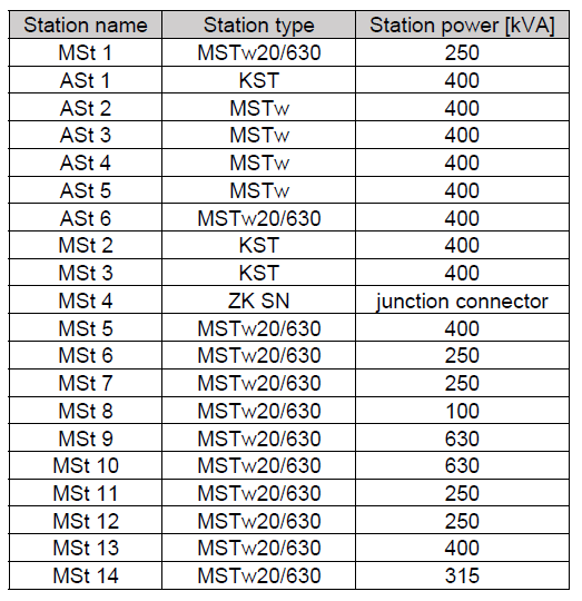
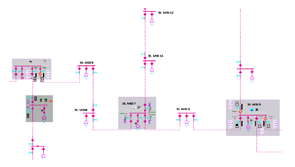
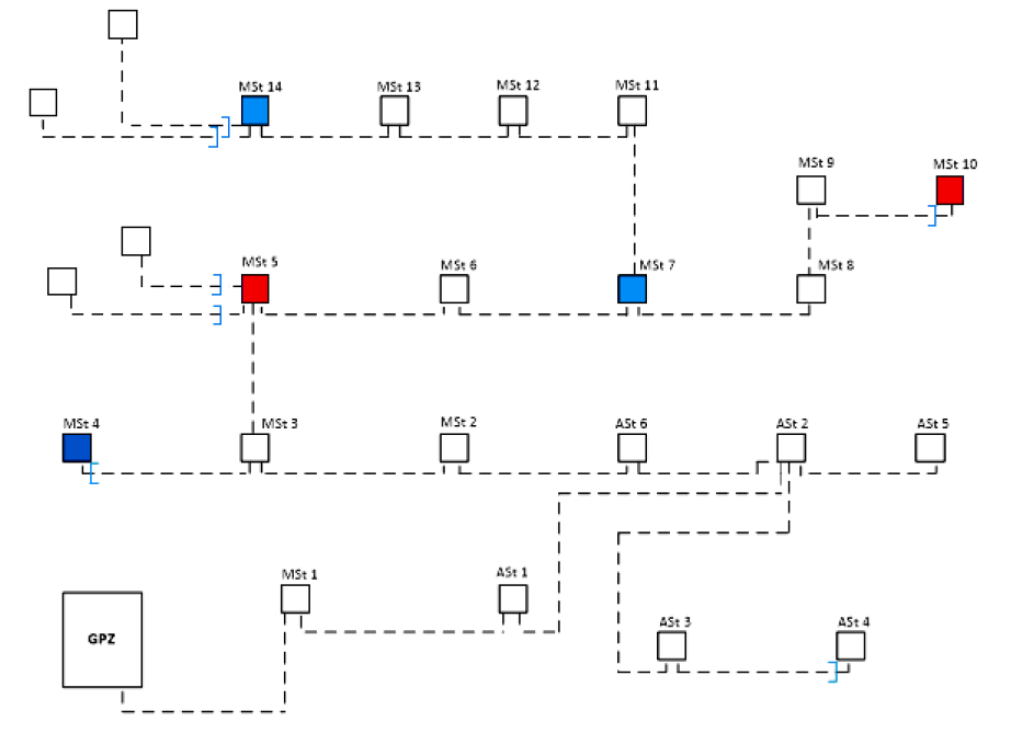
Fig.2 below presents the diagram of described cable run of a medium voltage line, the stations marked with blue colour allow to read voltage and current, the stations marked with red colour allow only to read current, division of a network was marked with blue brackets, in which, where necessary, the whole or part of described cable run can be supplied from adjacent lines.

In traditional networks, voltage and current load of specific lines could be tracked in the power supply points, that is, in the transformer/switching station at the beginning of a line.

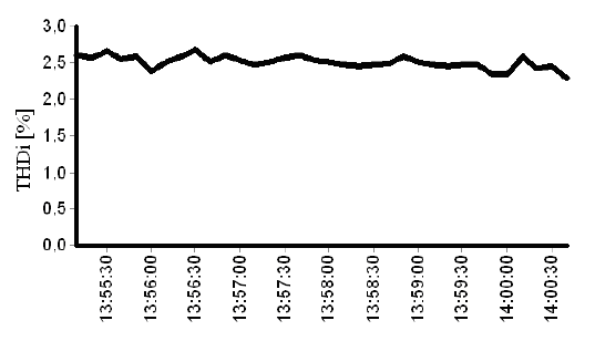
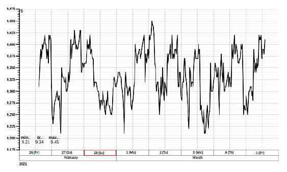
At present, we can track and archive voltage and load of selected medium voltage linear sequence inside the network, which was presented on below example of voltage tracking of the phase L1, for seven-day period of registration.

Fig.3. Measurement of voltage of the phase L1 in a transformer/switching station at the beginning of a line

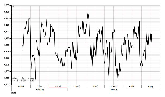
At the beginning of examined cable line, we can read voltage in the section tracks supplying cable run from the area of voltage measurement of 110/15 kV transformer / switching station, where registered measurement of voltage of the phase L1 was presented on fig.3.

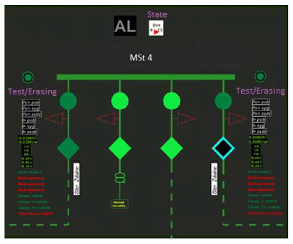
Another voltage measuring point is measurement in MSt. 4 station in the field direction towards MSt. 3 station. MSt. 4 station in SCADA system was presented on fig.4. In normal network layout, switch in this field is open, in the so-called “network division”, which can be closed when there is a need of planned switches in order to relieve the cable in linear sequence in a different section or damage to a cable and the use of voltage application during failure after elimination of a damaged cable.

Fig.4. MSt 4 station in SCADA system

Measurement of voltage presented on fig.5 was taken at the end of examined cable run, and its value shows the voltage in open switch. Comparing this value with the value presented above in an incoming feeder of a different cable run, we obtain knowledge of voltage value on both sides of an open switch. Such information is useful for DSO service before closing live switch to the ring and connection of two cable runs. Measurement of voltage in MSt. 4 presented below shows voltage of the phase L1 at a distance of 3610 m from the transformer/switching station supplying a cable run. The next point in an examined cable run is MSt. 7 station presented on fig.6., which is 1018 meters away from the transformer/switching station.

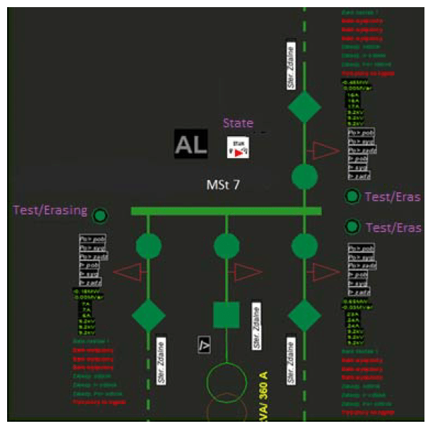
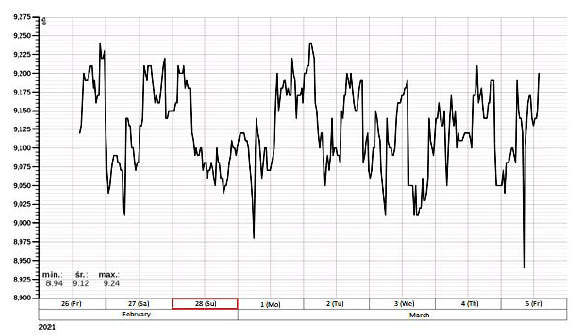
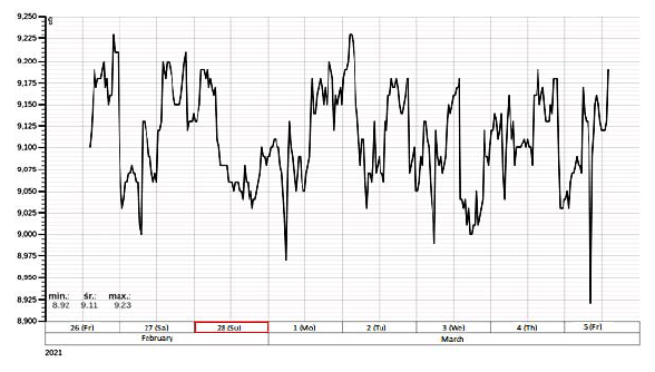
In this station, we can monitor voltage in an incoming feeder and two outgoing bays from the station. The measurements were presented on fig.7 and 8.

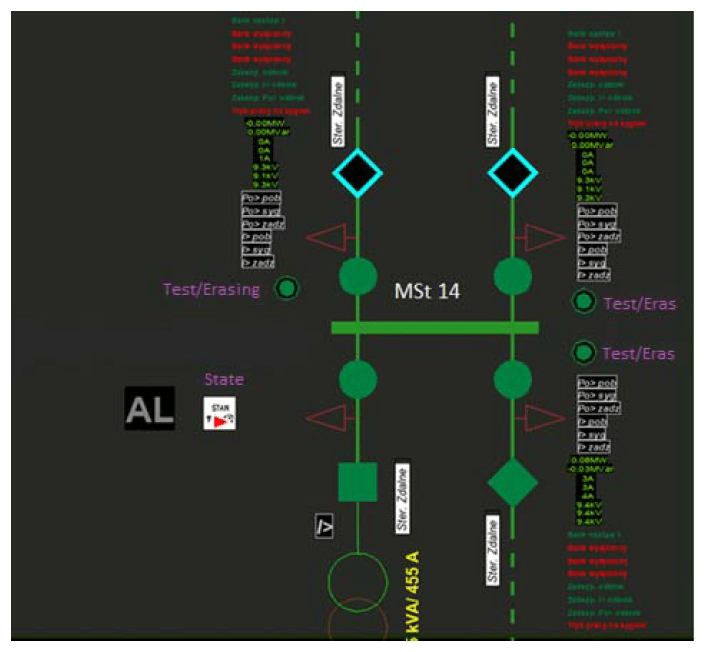
The last voltage measuring point in the examined cable run is MSt 14 station at the end of linear sequence, in which read voltage value is voltage at the end of a cable run, but also a voltage in the medium voltage/ low voltage transformer on the medium voltage side. It results from network scheduled layout, where switches in the outgoing bays in normal network layout are in open condition. MSt. 14 station in SCADA system was presented on fig.9. Measurement of voltage of the phase L1 in MSt 14 station was presented on fig.10.

Fig.5. Measurement of voltage of the phase L1 in MSt. 4 on the switch in division, marked with blue colour

Fig.6. MSt. 7 in SCADA system

Fig.7. Measurement of voltage of the phase L1 on inflow to MSt. 7 station, towards MSt

Fig.8. Measurement of voltage of the phase L1 on outflow of MSt. 7 station, towards MSt. 11

In this case, voltage value in open switches in the feeder bays is also necessary information about presence of voltage at the ends of adjacent cable runs and also its value and comparison with voltage in the inflow of the station, which is an important information before closing live switch to the ring.

Above measurements were enabled by development of technology connected with transformers and voltage and current sensors, as well as modern medium voltage switchgears with built-in devices making remote control by the Dispatcher possible and development of remote communication such as GPRS or TETRA.

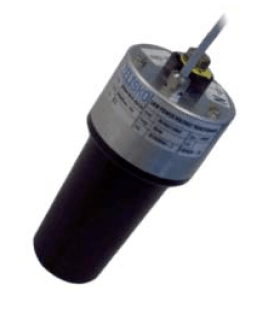
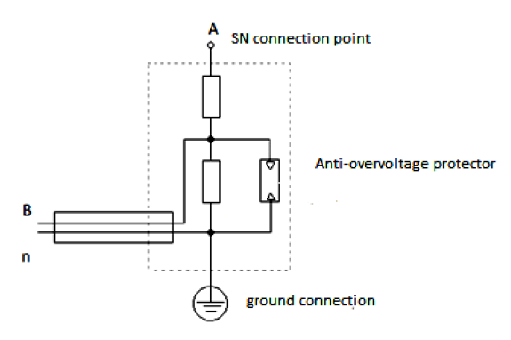
The remote measurements in the cable lines are taken in internal stations, using transformers for measurement of and current and voltage value, as well as voltage allocators and current sensors [3], which are more and more often applied in modern solutions of medium voltage switchgears. Fig.11 and 12 present physical view and equivalent diagram of a voltage sensor.

Fig.9. MSt. 14 station in SCADA system

Voltage sensor acts as a resistance divider that consists of two resistance elements that divide input signal so as to obtain normalized output signal. Thanks to surge arresters built in a sensor, connected measuring devices were secured.

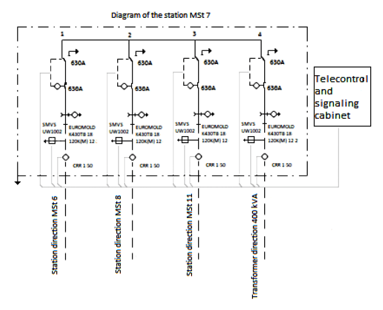
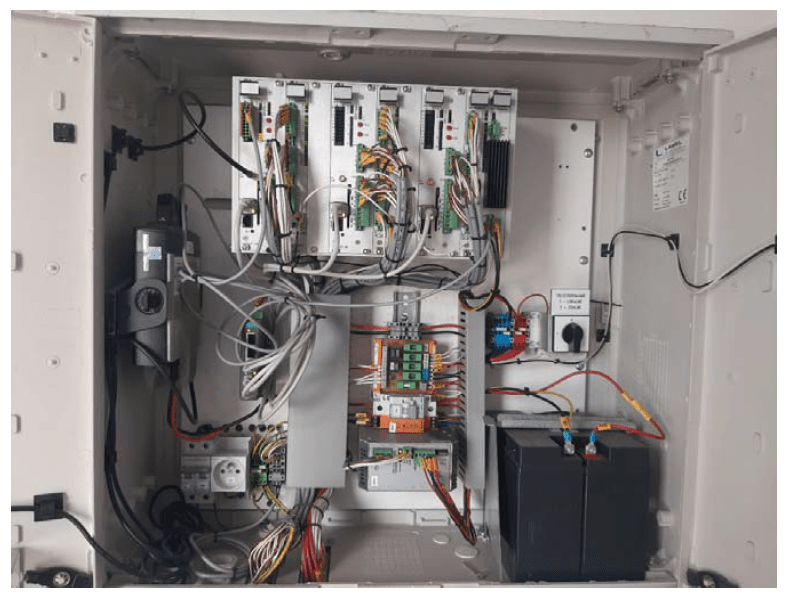
Fig. 13 below presents a diagram of connection of the sensors, whereas, fig.14. presents supply systems of the connectors built in the station marked on the diagram as – MSt. 7.

Fig.10. Measurement of voltage of the phase L1 in MSt 14 station, the end of a cable run

The measurement from voltage sensors in a specific feeder bay is sent through transmitter in a cabinet with a plant controller through antenna via transmission through GPRS and TETRA to telemechanic controller in a supervision centre [11,13].

Fig.11. Voltage sensor [22]

Fig.12. Schematic diagram of a voltage sensor [22]

Conclusions

Modern energy networks, thanks to their measuring capabilities, data collection, visualization of energy system participants, including producers, transmission, distribution and end consumers allow to integrate all participants and contribute to improvement of reliability of supplying electric energy of appropriate parameters and also largely increase energy efficiency. The functions of the energy networks mentioned above allow to define them as smart networks [4,7].

The replacement of traditional networks with smart networks is a complex and long-term process. These changes are caused by the change of power industry environment in the form of availability by the consumers of the devices of increased requirements when it comes to supply of energy of appropriate parameters, but also broadly developing activity connected with production of energy by the consumers. Constant growth of sources of energy inside the network causes changeable dynamics of changes of network operating conditions, depending on the amount of available sources of energy and power demand in a system.

Fig.13. Diagram in a supply system in MSt. 7 station

Fig.14. Cabinet with a controller and remote communication system

Moving measuring points inside the network makes network more observable due to an option of tracking of voltage value and current flow in specific sections, which is significant during work of dispatching service, which has information before changing planned network layout. Such option of reacting through switches of specific network sections, or sensitive consumers due to the parameters of delivered energy and quicker reaction through change of network configuration and switching the consumer to a section, in which does not occur, for example, voltage changes during failure location.

Measurement of voltage in a station in the connector, which is in division that voltage from both different cable runs comes to, gives the Dispatcher access to voltage value on both sides of a switch before closing it to the ring, the example was described above. In traditional networks, in which the Dispatcher had not access to voltage value on both sides of a switch, they worked intuitively comparing voltage in the power supply points and considering their length.

Different use of current measuring capabilities in the energy networks allows to compare voltage in the power supply points and at the end of linear sequence. A significant and practical feature of modern energy networks is the possibility of archiving of voltage measurements for further analysis in many network points due to generation through dispersed sources connected to a specific cable run. In view of growing legal awareness among the consumers of the quality and values that delivered energy should have, as well as potential claims from the consumers concerning inappropriate parameters, the possibility of analysis of measuring data both in the power supply points and inside the network, as well as in the very consumers is becoming increasingly significant for the Distribution System Operators.

According to the authors, constant development of dispersed sources in various network points will force the Distribution System Operators to develop smart networks, with growing capabilities of controlling particular elements, which affects power stoppages, but also construction of measuring points allowing to track the dynamics of voltage changes and network load. Archived data will also be significant, allowing to analyse the parameters of electric energy in various network points, in order to determine the possibility of connecting additional sources of energy or making a decision about the necessity of doing investment works connected, for example, with expansion of a network.

REFERENCES

[1] Bignucolo F., Caldon R., Prandoni V., Radial MV networks voltage regulation with distribution management system coordinated controller, Electric Power Systems Research, 78(4) (2008), 634-645, ISSN 0378-7796, https://doi.org/10.1016/j.epsr.2007.05.007
[2] Stojanović D., Korunović L., Milanović J., Dynamic load modelling based on measurements in medium voltage distribution network, Electric Power Systems Research, 78(2) (2008), 228-238, ISSN 0378-7796, https://doi.org/10.1016/j.epsr.2007.02.003
[3] Babś A., Kajda Ł., Nowe rozwiązania pomiarów napięć i prądów w sieciach inteligentnych. Wiadomości Elektrotechniczne, (2017), No. 9, 28-31
[4] Babś A., Automatyzacja sieci rozdzielczych jako podstawowy element sieci inteligentnych, Automatyka, Elektryka, Zakłócenia, 4 (2013), No. 1(12), 22-28
[5] Cataliotti A., Daidone A., Tine G., Power Line Communication in Medium Voltage Systems: Characterization of MV Cables, IEEE Transactions on Power Delivery, 23 (2008), No. 4, 1896-1902, https://doi.org/10.1109/TPWRD.2008.919048
[6] Al-Wakeel A., Wu J., Jenkins N., State estimation of medium voltage distribution networks using smart meter measurements, Applied Energy, 184 (2016), 207-218, ISSN 0306-2619, https://doi.org/10.1016/j.apenergy.2016.10.010
[7] Wizja wdrożenia sieci inteligentnej w ENERGA-OPERATOR SA w perspektywie do 2020 roku, (2011), Gdańsk
[8] Ożadowicz A., Mikoś Z., Grela J., Zintegrowane zdalne systemy pomiaru zużycia i jakości energii elektrycznej – technologiczne case study platformy Smart Metering. Napędy i Sterowanie, (2014), No. 6, 109-114
[9] Kryonidis G., Demoulias C., Papagiannis G., A new voltage control scheme for active medium-voltage (MV) networks, Electric Power Systems Research, 169, (2019), 53-64, ISSN 0378-7796, https://doi.org/10.1016/j.epsr.2018.12.014
[10] Brenna M., et al., Automatic Distributed Voltage Control Algorithm in Smart Grids Applications, IEEE Transactions on Smart Grid, 4 (2013), No. 2, 877-885, https://doi.org/10.1109/TSG.2012.2206412
[11] Mazierski M., Czarnobaj A., Automatyzacja sieci i innowacyjne systemy dyspozytorskie a niezawodność dostaw energii elektrycznej, Energia Elektryczna, 11 (2014)
[12] Dib M., Ramzi M., Nejmi A., Voltage regulation in the medium voltage distribution grid in the presence of renewable energy sources, Materials Today: Proceedings, 13(3) (2019), 739-745, ISSN 2214-7853, https://doi.org/10.1016/j.matpr.2019.04.035
[13] Dobrzyński K., Lubośny Z., Kluczni J., Noskie S., Falkowski D., Wykorzystanie infrastruktury systemu AMI w monitorowaniu i sterowaniu sieciami niskiego napięcia. Zeszyty Naukowe Wydziału Elektrotechniki i Automatyki Politechniki Gdańskiej, 53 (2017), 133-136, ISSN 2353-1290
[14] Świderski J., Dopierała P., Świniarski M., Bezpieczeństwo cybernetyczne transmisji danych pomiędzy systemami nadrzędnymi a telemetrycznymi sterownikami obiektowymi na potrzeby energetyki w świetle wymagań normy IEC 62351. Wiadomości Elektrotechniczne, 87 (2019), No.6, 4-9
[15] Neagu B., Grigoras G., Optimal Voltage Control in Power Distribution Networks Using an Adaptive On-Load Tap Changer Transformers Techniques, 2019 International Conference on Electromechanical and Energy Systems (SIELMEN), (2019), 1-6, https://doi.org/10.1109/SIELMEN.2019.8905904
[16] Kacejko P., Adamek S., Wancerz M., Jędrychowski R., Ocena możliwości opanowania podskoków napięcia w sieci nN o dużym nasyceniu mikroinstalacjami fotowoltaicznymi, Wiadomości elektrotechniczne, 85 (2017), No.9, 20-26
[17] Nakhodchi N., Busatto T., Bollen M., Measurements of Harmonic Voltages at Multiple Locations in LV and MV Networks, 2020 19th International Conference on Harmonics and Quality of Power (ICHQP), (2020), 1-5, https://doi.org/10.1109/ICHQP46026.2020.9177926
[18] Bolognani S., Bof N., Michelotti D., Muraro R., Schenato L., Identification of power distribution network topology via voltage correlation analysis, 52nd IEEE Conference on Decision and Control, (2013), 1659-1664, https://doi.org/10.1109/CDC.2013.6760120
[19] Abeysinghe S., Wu J., Sooriyabandara M., Abeysekera M., Xu T., Wang C., Topological properties of medium voltage electricity distribution networks, Applied Energy, 210 (2018), 1101-1112, ISSN 0306-2619, https://doi.org/10.1016/j.apenergy.2017.06.113
[20] Gao X., De Carne G., Liserre M., Vournas C., Voltage control by means of smart transformer in medium voltage feeder with distribution generation, 2017 IEEE Manchester PowerTech, (2017), 1-6, https://doi.org/10.1109/PTC.2017.7981001
[21] Łukasik Z., Kozyra J., Kuśmińska-Fijałkowska A., Monitoring of low voltage grids with the use of SAIDI indexes, Przegląd Elektrotechniczny, 93 (2017), No. 9,146-150, ISSN 0033-2097
[22] Sensory napięciowe i prądowe dla inteligentnych rozdzielnic średniego napięcia: http://www.zelisko.at


Authors: dr hab. inż. Jacek Kozyra, prof. UTH Rad., Uniwersytet Technologiczno-Humanistyczny im. Kazimierza Pułaskiego w Radomiu, Wydział Transportu, Elektrotechniki i Informatyki, ul. Malczewskiego 29, 26-600 Radom, E-mail: j.kozyra@uthrad.pl.; prof. dr hab. inż. Zbigniew Łukasik, Uniwersytet Technologiczno-Humanistyczny im. Kazimierza Pułaskiego w Radomiu, Wydział Transportu, Elektrotechniki i Informatyki, ul. Malczewskiego 29, 26-600 Radom, E-mail: z.lukasik@uthrad.pl; dr hab. inż. Aldona Kuśmińska-Fijałkowska, prof. UTH Rad., Uniwersytet Technologiczno-Humanistyczny im. Kazimierza Pułaskiego w Radomiu, Wydział Transportu, Elektrotechniki i Informatyki, ul. Malczewskiego 29, 26-600 Radom, E-mail:a.kusminska@uthrad.pl; mgr inż. Paweł Kaszuba, Volta Instalacje, Waldowo Szlacheckie, E-mail: pawel.kaszuba@vp.pl .


Source & Publisher Item Identifier: PRZEGLĄD ELEKTROTECHNICZNY, ISSN 0033-2097, R. 98 NR 10/2022. doi:10.15199/48.2022.10.67

Analysis of the Impact of Wind Turbine Power Characteristics on the Amount of Generated Energy

Published by Damian GŁUCHY1, Grzegorz TRZMIEL2, Poznan University of Technology
ORCID: 1. 0000-0003-2725-2614; 2. 0000-0002-3622-8889


Abstract. In the following article the impact of power characteristics of wind turbines on the total amount of generated power is introduced. The review of scientific literature suggested the need of further analysis of this issue. In order to do so, the performance parameters of eight wind turbines, 3kW each, were catalogued, their operational characteristics modeled, with the inclusion of sample measurements of essential environmental parameters, which were taken in exemplary location in Poland. Thanks to the gathered data, not only the wind speed histograms were made, but also the average wind speeds in particular months were calculated. Then, simulation studies were carried out to determine the most optimal wind turbine for a given location. The annual maximum amount of generated power served as the main criterion in the selection process. (Analiza wpływu charakterystyk mocy turbin wiatrowych na ilość wytwarzanej energii)

Streszczenie. W artykule przedstawiono wpływ charakterystyk mocy turbin wiatrowych na całkowitą ilość wytwarzanej mocy. Przegląd literatury naukowej wskazywał na potrzebę dalszej analizy tego zagadnienia. W tym celu skatalogowano parametry pracy ośmiu turbin wiatrowych o mocy 3kW każda, zamodelowano ich charakterystyki eksploatacyjne, uwzględniając przykładowe pomiary istotnych parametrów środowiskowych, które wykonano w przykładowej lokalizacji na terenie Polski. Dzięki zebranym danym wykonano nie tylko histogramy prędkości wiatru, ale również obliczono średnie prędkości wiatru w poszczególnych miesiącach. Następnie zrealizowano badania symulacyjne, które przeprowadzono w celu określenia najbardziej optymalnej turbiny wiatrowej dla danej lokalizacji. Głównym kryterium w procesie selekcji była roczna maksymalna ilość wytworzonej mocy.

Keywords: Wind turbine; Power characteristics modeling; Wind speed histogram; Wind turbine simulation.
Słowa kluczowe: turbina wiatrowa; modelowanie charakterystyk mocy; histogram prędkości wiatru; symulacja turbiny wiatrowej.

Introduction

Wind turbines, commonly referred to as wind generators are the type of the device which allows to transform the kinetic energy of wind into mechanical movement of turbine blades of the generator, creating electric energy as a result. Even though, the wind energy might seem to be wildly available, not every single corner of the Earth offers optimal conditions for the effective production of electric energy. Its total amount highly depends on various technical, performance parameters of the wind turbine and environmental conditions of the location, where the wind generator is placed. Only the proper analysis and mutual correlation of these factors can assure the quick return of incurred costs of the investment. This is especially important in the context of the use of wind turbines in distributed systems with energy storage, where implementation costs are significant. By appropriately matching the analyzed turbines to the location, the payback time for investment costs decreases, which allows to improve the profitability of the investment. In the case of investments in which energy storage and flexibly integrated renewable energy sources are used, it is the optimal selection of wind turbines that can bring the greatest savings to the overall economic balance. The best possible current use of electricity generated by wind turbines allows to limit the required capacity of energy storage, thus reducing investment and service costs. This is why the authors take up this problem as an important element of designing larger distributed systems for generating energy from RES with the possibility of its storage.

Many scientists try to precisely determine the performance parameters of the currently applied solutions worldwide [1-3], in terms of their cost-effectiveness in the field of wind energetics. Some e.g. [4, 21] tackle issues of strictly mechanical nature like selecting optimal machinery and the optimal adjustment of its parameters. Different solutions or propositions of update of the wind turbinecontrolled systems can be found in various publications [5- 10]. Nowadays, scientific research [11, 12] is more attentive to the problem of dispersion and diversification of wind sources in relation to maintaining stability and safety of the system designed to generate electric energy, as well as the need for analysis of potential damage of individual parts of the system e.g. planetary gears [13] or turbine blades [14, 15]. Ongoing tests of various [16, 17] with propositions for optimal energy storage solutions [18-20, 23]. It is worth noting that in the analyzes of the operation of wind turbines in specific wind conditions, histograms of wind speed and / or directions are often used [41, 43, 45, 46, 50]. A popular mathematical tool used to analyze the histograms of wind speed and generated energy is the Weibull distribution [42, 45, 46, 50, 51, 52, 53, 54, 55]. As can be seen, it is used for a variety of analytical tasks aimed at calculating current parameters, but also in modeling and predicting the operation of wind turbines and their components, often taking into account the stochastic nature of the processes taking place [52, 54, 55]. Histograms are also used e.g. in the analysis of vibrations of components of wind turbines, eg blades, in search of failure causes [44, 49] and in the modeling of wind conditions [47, 48]. All these actions are aimed to improve electric efficiency of the wind turbine system, its profitability and the reduction of time, necessary to return incurred costs of the investment.

The authors reviewed, among others of the abovementioned scientific articles, selectively used the tools and mathematical methods used there, and proposed an original procedure for solving the problem covered in the topic of the article for an example location in Poland. The authors of the following article decided to investigate the problem of selection of optimal wind turbines with different characteristics of power, currently available in retail. In order to maximize the amount of generated electric energy, various location types were taken into account, as shown in [22], not to mention the overall stability of wind conditions in a particular area. These aspects had to be taken into account to obtain accurate calculations regarding the maximum amount of generated energy [22] especially if such external factors always have the impact on the total amount of generated energy. Therefore, proper methodology to investigate the problem of optimization further were introduced, along with results of simulation research. The conducted research allowed to make the most optimal choice of specific solutions in different work conditions.

Generation of energy in wind turbines
1.1. Location conditions

Before any wind turbine is considered as a viable source of electric energy, first of all the location conditions had to be analyzed with a great caution due to their impact scale on the entire investment e.g. wind speed and its stability, because they are going to affect the performance of every wind turbine. Such analysis needs to include not only atmospheric conditions and latitude, but also factors which are not directly connected with climate, nor latitude. One of those factors is the ability to generation of heat and its later dissipation by seas and lands. It impacts the creation and movement of air masses. Topographic relief is important as well and must not be overlooked, due to its involvement in various orographic changes; e.g. mountain ranges, valleys or rivers. Vegetation might not be an orographic factor, but it has to be taken into the equation, because of its impact on the strength of wind. For instance, forest landscapes cause air distortions in the movement of air masses, while areas with less greenery do not exhibit create such distortions. The latitude itself determines so-called “latitude class”, which significantly impacts the amount of generated energy by wind turbines.

The characteristics of wind conditions of a particular locations can be achieved by measuring the speed and the direction of wind in specified time, it is highly advised to not take shorter period than one year in calculations. It allows to estimate the average wind speed and its stability in general. One must remember that these type of calculations must be conducted on 10 meters above the sea level. The wind speed differs, depending on the attitude where measurements are taken, therefore, all calculations are described by the function [24], where the measurement of the attitude hp in relation to the ground level must be conducted in a direct correlation to attitude of the turbine rotor ht.

.

where: α – latitude[-], vp – wind speed, where the measurement takes place hp [m/s], vt – wind speed on the attitude ht [m/s].

The change of wind speed is stochastic and its value heavily depends on atmospheric conditions, which makes the momentum difficult to utilize efficiently on a large scale. Even the analysis of multiple, annual measurements does not allow to make accurate estimation of average wind speed in later time periods with sufficient precise, Therefore, in the process of making the characteristics of energetic properties of wind, the Weibull distribution is used as a density function, which allows for the “probable” estimation of wind speed [25]:

.

where: pp(vw) – probable density [-], k – dimensionless shape factor (k>0) [-], c – scale factor (c>0) [-], γw – shift factor (in case of wind speed – γw=0)[-]).

The stochastic nature of generation of electric energy from wind turbines practically prohibits the effective utilization of wind energy in autonomous sources, connected to the receiver. It is a result of the lack of correlation between the energy demand and its later utilization. Therefore, wind turbines are often used with electro energy system, allowing to minimize the instability of power generation if the ratio of generated power by the wind turbine between the power of electro energy system is miniscule [26]. Alternatively, it is possible to assume the cooperation of wind farms with energy storage and optionally with other renewable energy sources, which is more and more common with distributed generation of electricity. In this case, the idea presented by the authors of this article does not change, namely the optimal use of the energy generated on a regular basis by the power plants allows to reduce the target capacity of the designed energy storage. Due to the complexity of this issue, this topic is beyond the scope of this publication. However, it should be remembered that the topic proposed by the authors is important both in systems without and with energy storage. Apart from its stochastic nature, wind energy also has a deterministic component related to periodic changes: day, seasons of the year and multi-year period. The first two cases can be considered by analyzing the measurements of wind energy resources separately for the spring-summer and autumn-winter periods, and by determining the average difference in wind energy for night and day. The multiple annual period is the most difficult to take into account due to the need to have detailed speed measurements for a specific location from many years. Regardless of the type of the determined deterministic component, the measurements must always be performed with a frequency sufficient to analyze the dynamics of wind energy changes.

1.2. Technical parameters of wind turbines

The performance parameters of the wind turbine define the final shape of the characteristics of power generation and its high dependence on the wind speed. Its nonlinear operation is a result of partial suppression of the flow of the stream of air which decreases energy generation and the speed of the wind; described in the following equation [27]:

.

where: Pt – mechanical power of the wind turbine [W], Pw – the power in the stream of air [W], cp(λ) – Betz factor, which serves as sort of correction of the theoretical value – tip-speed ratio. λ [-].

The power of the air stream can be described with the following equation [28]:

.

where:, ρ – density of air [kg/m3], A – the surface area with the inclusion of blade coverage surface of the wind turbine [m2], vw – wind speed [m/s]. The tip-speed can be described with the following equation [29]:

.

where: ω – angular velocity of the turbine rotor [rad/s], R – the rotor radius [m].

The Betz factor in the function describes the tip speed for various wind turbine rotors is shown in Figure I. Its maximal value never exceeds 0.6, which is caused by various states of aerodynamic, based on the construction of the particular wind turbine e.g. number of blades or shape of the rotor itself.

The above values are strictly theoretical, therefore, it is advised to use the characteristics provided by the manufacturer of the wind turbine which should be included in catalog in the form of a table. It is a result of the measurements conducted on an actual location.

Fig.1. The changes of aerodynamic state of the rotor in the function of tip-speed [30]

2. The analysis of wind conditions of a selected location regarding the usage of wind turbines

The analysis of a selected location was started 30 kilometers from the Rzeszow city in Poland, and naturally all kinds of orographic conditions had been taken into account in order to accurately determine wind conditions within the selected area. The measurements are taken from the database of the private owner of the wind turbines who agreed to use it in the publication. To do so, the average wind speed for each month had to be measured with a time step of 47 seconds (one year, 2011). The research was conducted in an ongoing manner on the height of 10 meters, allowing the creation of the detailed database, which included many useful parameters such as: date, time, average speed, atmospheric pressure or wind direction and its temperature. The gathered information was further analyzed, which was crucial to obtain accurate calculations regarding the average wind speed for every month of the year (shown in Figure 2), not to mention the average wind speed for as a whole, which equaled 5.7 m/s.

Fig.2. The average wind speed for every month in 2011

These analysis allow for the perinatal determination of wind conditions (capabilities) of the selected area, however, they do not provide any kind of feedback about the turbine type, which would be optimal for a desired area. Therefore, the next step was to pinpoint the frequency distribution of the particular wind speed. It was achieved by making a histogram, which is the density of probability of particular wind speed to occur – created by summing up 47 second wind events of particular strength e.g. for 1 m/s, the range between 0.5 to 1.4 m/s was taken into the equation.

Instead of a detailed showcase of the database of wind speed which is not only quite vast, but also difficult to analyze, it is better to describe wind conditions by a histogram. Such approach allows to select the optimal type of wind turbine much quicker. In order to make the whole process of modeling wind conditions even more effective, the Weibull function can be used to reduce the necessary calculations [31]. Such calculations were made for the histogram of wind speed, which was based on individual calculations, done by the authors of the following article; as shown in Figure 3.

Fig.3. The histogram of wind speed, based on the Weibull distribution of wind speed

3. Modeling of selected wind turbines

The determination of the wind turbine models was performed in the MS Visual Studio environment. It involved the implementation of eight wind turbines from different manufacturers with a power of 3 kW each, in table form with a time step for every 1 m/s. The following information was obtained from catalog notes from the websites of individual producers [32 – 39]. Visualization of individual power characteristics is presented in Figure 4.

Fig.4. Power characteristics for eight wind turbines modeled in the MS Visual Studio environment with 3 kW rated power [own source]

The selected cases for the database include both turbines with vertical and horizontal rotor axis of rotation. At the same time, it is important to emphasize the confusing “diversity” in terms of interpretation of technical parameters by the manufactures of wind turbines. The rated power of the turbine is usually the maximum power achieved at a certain wind speed, kept to the cutout speed, as shown in various scientific publications. However, most manufactures give only approximate values. In all investigated cases, the value of generated power by the turbine was much higher than the one given by the manufacturer (3 kW). (by several, or even several dozen percent). In addition, in their catalog notes focus on presenting the slope of the characteristic of power rise, ignoring the behavior of the generator when it exceeds the rated power speed. In this area, turbines are often subjected to decelerate artificially. The generated power decreases when the wind power is increasing.

Power characteristics are given by manufacturers usually in a tabular form, with a wind speed step every 1 m / s. In order to obtain continuity of these characteristics, the least approximation of squares was used with the exponential function [40]. This allowed to achieve the so-called “golden mean” between the accuracy of calculations and the time necessary to obtain them.

4. Simulation of work of modeled wind turbines in the conditions of the tested location

The simulation of modeled wind turbines was performed by using two methods: based on a wind speed histogram and directly using wind speed measurements from a database. In both cases, it was necessary to take the height of the mast into account, which was made by using the vertical wind profile [22,24] described in formula 1.

The simulation based on the wind histogram was performed by searching for the best possible correlation between the production characteristics and the wind speed histogram. The generator is selected in a way that its characteristics of Pel=f(vw), could coincide with the most common wind speeds. From the simulation point of view, an algorithm was created, which showed the percentage annual share of rated power of the turbine, based on the wind histogram and modeled characteristics of wind turbine. On its basis, the average annual amount of produced energy was determined. Both of these values for individual wind turbines are presented in Table 1 (column 3 and 4). The highest value of generated energy indicates the best adjustment of the turbine parameters in relation to wind conditions in a particular location. At the same time, it should be noted that selecting the most optimal solution is burdened by the potential error, which is a result of rounding the numbers used to create the histogram. In case of the application created by the authors to determine the probability of speed occurrence, e.g. 1 m/s, all cases of speed occurrence in the range from 0.5 m/s to 1.4 m/s inclusive are included.

A much more accurate value of energy obtained from a wind turbine can be obtained by using the power characteristics and wind speed samples in the simulation. Accuracy can be additionally increased if the averaging time ΔtTW for one sample is as short as possible. The amount of ATW electricity generated by a specific type of wind turbine was determined from the dependence 6. The results of the simulation were also presented in Table 1 (column 2).

.

where: N – number of measurement samples, PTW(vw) – wind turbine power for the n-th measurement sample (wind speed is equal to vw)[W], ΔtTW – time step for measuring wind speed [s].

Table 1. Average annual energy value generated on the basis of power characteristics by wind turbines of various manufacturers [own study]

.

From the analysis of the results presented in Table 1, it can be concluded that the average annual energy yields obtained by the two simulation methods described above are very similar. This means that for a given location, the turbine which generates the highest power can be selected, based on the wind speed measurement and the histogram. The second of these methods is much simpler to implement, due to the use of wind speed probability distribution rather than an extensive measurement database. From the point of view of the algorithm, it is also much faster due to the smaller number of operations performed. In the presented location, the best in 2011 would be BOF-V turbine with its power of approx. 30%, provides a satisfactory result.

In extreme cases: the best and worst correlation between wind power and speed characteristics shows a 60% difference in terms of generated electricity. The reason for such a large discrepancy in annual energy yields can be presented in the form of a graph of the amount of energy generated annually in given wind speed ranges, as shown in Figure 5. This disproportion indicates the importance of earlier analysis of wind conditions in correlation with the characteristics of wind turbines.

Fig.5. Characteristics of the amount of energy generated during the year from individual windiness ranges for the TypBr-V and BOF-V turbines [own source]

5. Conclusions

Based on the research, modeling and simulation carried out, the authors analyzed the impact of wind turbine power characteristics on the amount of energy generated in a given location. The result is an unequivocal demonstration of the need to gather information about windiness and the environmental parameters of a particular location before investing in wind turbines. Such archived information should be saved in the form of a database or histogram of wind speed, for later processing with the participation of wind turbine power characteristics. Irrespective of the simulation method chosen from the two used by the authors, the amount of energy generated from each of the considered wind turbines can be obtained. Appropriate selection of wind turbines for the location allows to reduce the capacity of the designed energy storage in distributed generation systems containing integrated RES, thus reducing investment and service costs. Thus, the proposed subject of the article is universal, regardless of the target concept of a distribution network, including any generation systems and, optionally, energy storage.

Funding: This research was funded by Polish Government, grant number [0212/SPAD/0512].
Conflicts of Interest: The authors declare no conflict of interests.

REFERENCES
[1] Pfaffel S., Faulstich S., Kurt R., Performance and reliability of wind turbines: A review, Energies 10.11 (2017): 1904, https://doi.org/10.3390/en10111904
[2] Hyeonwu K., Bumsuk K., Wind resource assessment and comparative economic analysis using AMOS data on a 30 MW wind farm at Yulchon district in Korea, Renewable Energy 85 (2016): 96- 103, https://doi.org/10.1016/j.renene.2015.06.039
[3] Garcia-Sanz M., A Metric Space with LCOE Isolines for Research Guidance in wind and hydrokinetic energy systems, Wind Energy 23.2 (2020): 291-311, https://doi.org/10.1002/we.2429
[4] Tafticht, T., et al., Output power maximization of a permanent magnet synchronous generator based stand-alone wind turbine, 2006 IEEE International Symposium on Industrial Electronics. Vol. 3. IEEE, 2006
[5] Morimoto S., et al., Sensorless output maximization control for variable-speed wind generation system using IPMSG, IEEE Transactions on Industry Applications 41.1 (2005): 60-67
[6] Errami Y., Ouassaid M., Maarouf M., Control of a PMSG based wind energy generation system for power maximization and grid fault conditions, Energy Procedia 42 (2013): 220-229
[7] Corradini M.L., Letizia M., Ippoliti G., Orlando G., Fully sensorless robust control of variable-speed wind turbines for efficiency maximization, Automatica 49.10 (2013): 3023-3031
[8] Yaramasu V., Wu B., Predictive control of a three-level boost converter and an NPC inverter for high-power PMSG-based medium voltage wind energy conversion systems, IEEE Transactions on Power Electronics 29.10 (2013): 5308-5322
[9] Gebraad P., et al., Maximization of the annual energy production of wind power plants by optimization of layout and yaw-based wake control, Wind Energy 20.1 (2017): 97-107
[10] Park J., Law K.H.. Bayesian ascent: A data-driven optimization scheme for real-time control with application to wind farm power maximization, IEEE Transactions on Control Systems Technology 24.5 (2016): 1655-1668
[11] Li X., Diversification and localization of energy systems for sustainable development and energy security, Energy policy 33.17 (2005): 2237-2243
[12] Liljenfeldt J., Pettersson O., Distributional justice in Swedish wind power development – An odds ratio analysis of windmill localization and local residents’ socio-economic characteristics, Energy Policy 105 (2017): 648-657
[13] Zhang Y., Lu W., Chu F., Planet gear fault localization for wind turbine gearbox using acoustic emission signals, Renewable Energy 109 (2017): 449-460
[14] Arnold P., et al., Radar-based structural health monitoring of wind turbine blades: The case of damage localization, Wind Energy 21.8 (2018): 676-680
[15] Park B., et al., Delamination localization in wind turbine blades based on adaptive time-of-flight analysis of noncontact laser ultrasonic signals, Nondestructive Testing and Evaluation 32.1 (2017): 1-20
[16] Campagnolo F., et al., Wind tunnel testing of a closed-loop wake deflection controller for wind farm power maximization, Journal of Physics: Conference Series. Vol. 753. No. 3. IOP Publishing, 2016
[17] Campagnolo, F., et al., Wind tunnel testing of power maximization control strategies applied to a multi-turbine floating wind power platform, The 26th International Ocean and Polar Engineering Conference. International Society of Offshore and Polar Engineers (2016)
[18] Tomczewski A., Kasprzyk L., Nadolny Z., Reduction of power production costs in a wind power plant–flywheel energy storage system arrangement, Energies 12.10 (2019): 1942
[19] Tomczewski A., Kasprzyk L., Optimisation of the structure of a wind farm—Kinetic energy storage for improving the reliability of electricity supplies, Applied Sciences 8.9 (2018): 1439
[20] Hemmati R., Technical and economic analysis of home energy management system incorporating small-scale wind turbine and battery energy storage system, Journal of Cleaner Production 159 (2017): 106-118
[21] Śliwiński A., Wróbel K., Tomczewski K., Tomczewski A., Impact of winding parameters of a switched reluctance generator on energy efficiency of a wind turbine, SME (2018), https://ieeexplore.ieee.org/document/8442592, DOI: 10.1109/ISEM.2018.8442592
[22] Wrobel K., Tomczewski K., Sliwinski A., Tomczewski A., The Impact of a Wind Turbine Characteristics on the Annual Energy Performance at Given Wind Speed Distribution, PTZE (2018), https://ieeexplore.ieee.org/document/8503230, DOI: 10.1109/PTZE.2018.8503230
[23] Kasprzyk L., Tomczewski, A., Bednarek K., Bugała A., Minimisation of the LCOE for the hybrid power supply system with the lead-acid battery, In E3S Web of Conferences (Vol. 19, p. 01030). EDP Sciences, EEMS (2017), DOI: 10.1051/e3sconf/20171901030
[24] Błasiński W.. Simulator low-power wind turbine (in Polish), Przegląd Elektrotechniczny No. 12 (2017): 263-265
[25] Patel M.R.. Wind and Solar Power Systems: Design, Analysis, and Operation. Second Edition, Taylor & Francis Group (2006)
[26] Malko J., Prediction of wind farm generation capacity (in Polish), Przegląd Elektrotechniczny No.9 (2008): 65-67
[27] Uracz P., Karolewski B., Modeling of wind turbines with the use of power factor characteristics (in Polish), Prace Naukowe Instytutu Maszyn, Napędów i Pomiarów Elektrycznych 59 (2006), Wrocław: Wydawnictwo Politechniki Wrocławskiej
[28] Soliński I., Energy and economic aspects of the use of wind energy (In Polish), Wyd. Inst. Gospodarki Surowcami Mineralnymi i Energią PAN (1999), Krakow
[29] Jarek G., Jeleń M., Gierlotka K., Wind turbine simulator based on a DC motor (in Polish), Przegląd Elektrotechniczny (6), 2014
[30] Numerical Investigation of the Savonius Vertical Axis Wind Turbine and Evaluation of the Effect of the Overlap Parameter in Both Horizontal and Vertical Directions on Its Performance, https://www.mdpi.com/2073-8994/11/6/821/xml
[31] Kumar D., Chatterjee K., A review of conventional and advanced MPPT algorithms for wind energy systems, Renewable and sustainable energy reviews (2016): 957-970
[32] https://www.brasit.pl/turbina-wiatrowa-typbr-v-3kw/ (accessed 21.05.2020)
[33] https://www.brasit.pl/aeolos-v-3000w/ (accessed 21.05.2020)
[34] https://www.brasit.pl/pionowa-elektrownia-wiatrowa-buf-v-3kw/ (accessed 21.05.2020)
[35] https://www.brasit.pl/pionowa-elektrownia-wiatrowa-saw-v-3kw/ (accessed 21.05.2020)
[36] https://www.brasit.pl/elektrownia-wiatrowa-turbina-hy-h-3kw/ (accessed 21.05.2020)
[37] https://www.brasit.pl/elektrownia-wiatrowa-turbina-humbr-h-3kw/ (accessed 21.05.2020)
[38] https://ekotaniej.pl/media/wysiwyg/karta-turbina.pdf (accessed 21.05.2020)
[39] http://hipar.pl/ecorote-2800/ (accessed 21.05.2020)
[40] Thapar V., Agnihotri G., Sethi V.K., Critical analysis of methods for mathematical modelling of wind turbines, Renewable Energy, vol. 36 (2011), no. 11, pp. 3166-3177
[41] Paulsen B.M., Schroeder J.L., An examination of tropical and extratropical gust factors and the associated wind speed histograms, Journal of Applied Meteorology 44.2 (2005): 270-280
[42] Carta J.A., Ramirez P., Velazquez S., A review of wind speed probability distributions used in wind energy analysis: Case studies in the Canary Islands, Renewable and sustainable energy reviews 13.5 (2009): 933-955
[43] Sohoni V., Gupta S, Nema R., A comparative analysis of wind speed probability distributions for wind power assessment of four sites, Turkish Journal of Electrical Engineering & Computer Sciences 24.6 (2016): 4724-4735
[44] Joshuva A., Sugumaran V., A study of various blade fault conditions on a wind turbine using vibration signals through histogram features, Journal of Engineering Science and Technology 13.1 (2018): 102-121
[45] Sarkar A., Gugliani G., Deep S., Weibull model for wind speed data analysis of different locations in India, KSCE Journal of Civil engineering 21.7 (2017): 2764-2776
[46] Gugliani G. K., et al., New methods to assess wind resources in terms of wind speed, load, power and direction, Renewable Energy 129 (2018): 168-182
[47] Zárate-Miñano R., Anghel M., Milano F., Continuous wind speed models based on stochastic differential equations, Applied Energy 104 (2013): 42-49
[48] Chen X., Huang W., Yao G., Wind speed estimation from X-band marine radar images using support vector regression method, IEEE Geoscience and Remote Sensing Letters 15.9 (2018): 1312-1316
[49] Yu Y., et al., Image-based damage recognition of wind turbine blades, 2017 2nd International Conference on Advanced Robotics and Mechatronics (ICARM), IEEE
[50] El-Asha S., Zhan L., Iungo G.V., Quantification of power losses due to wind turbine wake interactions through SCADA, meteorological and wind LiDAR data, Wind Energy 20.11 (2017): 1823-1839
[51] Sedaghat A., et al., Determination of rated wind speed for maximum annual energy production of variable speed wind turbines, Applied energy 205 (2017): 781-789
[52] Seo S., Si-Doek O., Ho-Young K., Wind turbine power curve modeling using maximum likelihood estimation method, Renewable energy 136 (2019): 1164-1169
[53] Soulouknga M. H., et al., Analysis of wind speed data and wind energy potential in Faya-Largeau, Chad, using Weibull distribution, Renewable energy 121 (2018): 1-8
[54] Asghar A.B., Liu X., Estimation of wind speed probability distribution and wind energy potential using adaptive neuro-fuzzy methodology, Neurocomputing 287 (2018): 58-67
[55] Horn J.T., Leira B.J., Fatigue reliability assessment of offshore wind turbines with stochastic availability, Reliability Engineering & System Safety 191 (2019): 106550


Authors: dr inż. GrzegorzTrzmiel, Politechnika Poznańska, Instytut Elektrotechniki i Elektroniki Przemysłowej, ul. Piotrowo 3a, 60-965 Poznań, E-mail: Grzegorz.Trzmiel@put.poznan.pl; mgr inż. Damian Głuchy, Politechnika Poznańska, Instytut Elektrotechniki i Elektroniki Przemysłowej, ul. Piotrowo 3a, 60-965 Poznań, E-mail: Damian.Gluchy@put.poznan.pl.


Source & Publisher Item Identifier: PRZEGLĄD ELEKTROTECHNICZNY, ISSN 0033-2097, R. 98 NR 11/2022. doi:10.15199/48.2022.11.60

A Photovoltaic System Maximum Power Point Tracking by using Artificial Neural Network

Published by KARRI HEMANTH KUMAR1, GADI VENKATA SIVA KRISHNA RAO2, Department of Electrical Engineering, Andhra university college of Engineering (A), Andhra university, Vishakhapatnam, India. ORCID: 1. 0000-0001-6198-999X. ORCID: 2. 0000-0003-4314-4816


Abstract: The electrical energy from the sun can be extracted using solar photovoltaic (PV) modules. This energy can be maximized if the connected load resistance matches that of the PV panel. In search of the optimum matching between the PV and the load resistance, the maximum power point tracking (MPPT) technique offers considerable potential. This paper aims to show how the modelling process of an efficient PV system with a DC load can be achieved using an artificial neural network (ANN) controller. This is applied via an innovative methodology, which senses the irradiance and temperature of the PV panel and produces an optimal value of duty ration for the boost converter to obtain the MPPT. The coefficients of this controller have been refined based upon previous data sets using the irradiance and temperature. A gradient descent algorithm is employed to improve the parameters of the ANN controller to achieve an optimal response. The validity of the PV system using the MPPT technique based on the ANN controller is further demonstrated via a series of experimental tests at different ambient conditions. The simulation results show how the MPPT technique based on the ANN controller is more effective in maintaining the optimal power values compared with conventional techniques.

Streszczenie. Energia elektryczna ze słońca może być pozyskiwana za pomocą modułów fotowoltaicznych (PV). Energię tę można zmaksymalizować, jeśli rezystancja podłączonego obciążenia jest zgodna z rezystancją panelu fotowoltaicznego. W poszukiwaniu optymalnego dopasowania między PV a rezystancją obciążenia, technika śledzenia punktu maksymalnej mocy (MPPT) oferuje znaczny potencjał. Niniejszy artykuł ma na celu pokazanie, w jaki sposób można osiągnąć proces modelowania wydajnego systemu fotowoltaicznego z obciążeniem DC przy użyciu kontrolera sztucznej sieci neuronowej (ANN). Jest to stosowane za pomocą innowacyjnej metodologii, która wykrywa natężenie promieniowania i temperaturę panelu fotowoltaicznego i wytwarza optymalną wartość współczynnika wypełnienia dla konwertera doładowania w celu uzyskania MPPT. Współczynniki tego kontrolera zostały udoskonalone w oparciu o poprzednie zestawy danych z wykorzystaniem natężenia promieniowania i temperatury. Algorytm opadania gradientu jest wykorzystywany do poprawy parametrów kontrolera ANN w celu uzyskania optymalnej odpowiedzi. Ważność systemu fotowoltaicznego wykorzystującego technikę MPPT opartą na sterowniku ANN jest dalej demonstrowana w serii testów eksperymentalnych w różnych warunkach otoczenia. Wyniki symulacji pokazują, w jaki sposób technika MPPT oparta na sterowniku ANN skuteczniej utrzymuje optymalne wartości mocy w porównaniu z technikami konwencjonalnymi. (Śledzenie maksymalnego punktu mocy systemu fotowoltaicznego za pomocą sztucznej sieci neuronowej)

Key words: Photovoltaic System, Maximum Power Point Tracking, Artificial Neural Network.
Słowa kluczowe: Saystem fotowoltaiczny, śledzenie maksymalnej mocy, sieć neuronowa

Introduction

Increasing the energy demand around the world has focused attention on the need to develop renewable sustainable sources with minimal environmental impact. Of all the potential renewable sources of energy, that derived from solar power continues to grow in prominence as it can be utilized to generate electrical power without pollution and is readily available around the globe. Most significantly, although the cost of installation is still prohibitive [1,2], once operational, the cost of the operation and maintenance is relatively low and commercially competitive with other available power sources. A key aspect of the solar cell is that it is a not-fixed voltage or current source, and thus depends upon the variation in irradiation, temperature, and load. Therefore, the overall efficiency of the solar array can be considerably low due to these variations. In order to ameliorate the efficiency of the solar cells, the maximum power point tracking (MPPT) technique is utilized to enhance the output. This technique is able to obtain the maximum possible power from a varying source by using a controlled DC-DC converter with a unique tracking algorithm introduced between the photovoltaic (PV) array the load [2].

Many MPPT techniques have been presented in the literature [1, 3, 4] including: Incremental Conductance (IC), Perturb and Observe (P and O), and the Feedback Linearization Method. However, most of them have limitations due to the non-linear characteristics of PV cells. More recently, intelligent techniques employing neural network and fuzzy logic are presented as an effective approach to trace the maximum power from the PV cells commensurate with changing atmospheric conditions [5–8]. Such intelligent techniques based on MPPT provide the facility to achieve a faster response with greater accuracy compared with conventional techniques. In this paper, a fuzzy neural network (FNN) controller based on the MPPT technique has been designed and implemented to control the duty cycle of a boost converter and to elicit the maximum power from the PV cells. The integrating of fuzzy logic with a neural network is more convenient for MPPT compared with conventional controllers by overcoming the limitations of the individual techniques. In particular, this offers higher accuracy with the non-linear behaviour of PV cells. The parameters of the FNN controller are also refined using a gradient descent-based back-propagation algorithm to obtain the optimal results.

Fig.1. Single diode model

PV cell

A PV cell mutates solar energy into DC electrical power via a physical operation known as the photoelectric elect. A PV array is composed of a number of PV cells connected in series and parallel to increment the voltage and current in the array. There are several variations of PV cell models [5,7,9] available to potential users. The classifications of these models depend on many factors, like the irradiation, temperature, elect of shadow, and the cell deviation from the diode operation [8,10]. In this paper, an approach has been adopted to use a single-diode model to represent the PV cell. This can then be modelled by a current source in anti-parallel circuit with a diode. In addition, parallel and series resistances are also included due to leakage current and resistances, as depicted in

.

where, 𝐈𝐃 is Diode Current; 𝐈𝐏𝐇 is Photon Current; 𝐈𝐩 is Current through Resistance 𝑹𝑺𝒉 ; 𝐈𝐩𝐯 is Photo Voltaic Current; 𝑹𝑺𝒉 is Shunt resistance; 𝑹𝑺 is Series resistance; 𝐈𝐩𝐯 is Photo Voltaic Voltage; 𝑰𝒐 Diode Saturation Current; 𝑽𝑫 is Diode Voltage; 𝜶 is Boltzmen’s Constant; 𝑽𝑻 is Terminal Voltage

Below mentioned diagrams Fig (2), Fig (3) shows the P-V curve and I-V curve of PV cell respectively.

Fig.2. P-V curve of PV cell
Fig.3. I-V curve of PV cell
Boost converter

The core of the MPPT strategy is a DC-DC converter. A DC-DC converter is utilized to transfer the maximum power of solar array to the load side, ensuring that maximum power has been transferred. In this work, the boost converter is utilized to vary the output voltage by adjusting the duty cycle to elicit the maximum power from the solar array, as depicted in Fig.4. The duty cycle of the boost converter is controlled by using the MPPT algorithm. This converter can be designed and modelled to operate at current-continuous mode (CCM) using the following equations.

Fig.4. Boost Converter where: 𝑉in is Input Voltage; L is Inductance; C is Capacitance; 𝑉out is output Voltage; 𝑖o is output Current

MPPT technique

The MPPT technique is utilized to obtain the maximum power and efficiency from the solar panel. This consists of a DC-DC converter that interconnects between the PV panel and the load and controller. The photovoltaic modules are not fixed electrical sources and the I–V characteristics are non-linear. This makes it more difficult for utilizing to provide the energy to any load. This is achieved by utilizing a boost converter which can be controlled by varying the duty cycle through an MPPT algorithm [1, 4, 9]. The MPPT controller changes the resistance, as seen from the PV panel, changing the duty cycle of the boost converter, and hence compels the PV panel to extract MPP to the load. In recent years, several techniques have been developed which can effectively track the MPPT.

Fuzzy Neural Network (FNN)

Controller The combination between fuzzy logic and the neural network over the advantages of both networks (human-like IF-THEN rules thinking, ease of incorporating expert knowledge, learning abilities, optimization abilities, and connectionist structures). For the present work, the fuzzy neural network controller is utilized to overcome the drawbacks of the individual techniques and control the PV output power to extract MPP. The FNN can thus be considered as a hybrid form of the neural network, with similarities to the general structure, but having special connections and node operations within the network. The FNN controller consists of a four-layer neural network based on fuzzy logic with an optimization algorithm for learning the neural network. The basic function of each layer is described.

Simulation results MPPT PV control system with artificial neural network

ANN technique is used with MPPT to optimize the response of the MPPT, in order to increase the efficiency of PV module. The structure of the system which is utilized in this paper is presented in Fig.5.

Fig.5. The proposed PV control system Where: T is Temperature; Ir is Solar Irradiance; L is Inductance; C is Capacitance

Modelling booster converter

The output DC voltage of the boost converter is greater than the input DC voltage. Consequently, from the equations were shown in previous sections, a DC-DC boost converter model is designed and applied using MATLAB/SIMULINK.

The design specifications of boost converter are shown in table 1. The specifications are for a variable value of the input voltage of the boost converter where the input voltage comes from the renewable source and the output voltage of boost converter is fixed to 45V DC.

Table 1. Specification of Boost Controller.

.
PV control system using ANN

The output characteristics of the two cases of PV module are nonlinear; moreover, the solar irradiance is changed continuously and unpredictable, so the maximum power point varied continuously, as seen in Fig.6.

Fig.6. Varying of MPP of PV module under different radiation and temperature

Fig.7. ANN architecture

In this paper, it can implement an ANN technique for tracking the maximum output power of the PV modules by commanding the boost converter. The architecture of ANN was shown in Fig.7. It is having Solar Irradiance, Temperature as input and Pulse input to IGBT as output. To design an ANN model, firstly according to the “nnstart” or “nntool” functions is used to create the ANN model. The proposed ANN in this paper is a multilayer feed forward back propagation NN, which consist of two layers which are hidden layer and output layer. Inputs on this design are irradiance and temperature also the output of the ANN model is a voltage at maximum power. Neurons number in each layer and structure of multilayer feed forward propagation NN are mostly variable and thus determined by experience and trial and error. So many of the trials are implemented until reaching the best design. And the final design consists of hidden layer constructed of 5 neurons whose activation function is a tangent sigmoid and the output layer has 1 neuron which activation function is a pure linear transfer function. The “trainlm” tool at MATLAB is used to train the ANN using Levenberg-Marquardt, so the ANN is trained to discover the relationship between inputs (irradiation and temperature) and the output (maximum voltage) as shown in Fig.8.

Fig.8. Training neural network
Fig.9. Training result of ANN block
Fig.10. The plot training state for ANN

Three kinds of samples are implemented on the ANN model training samples, validation samples for measuring NN generalization and testing samples for measuring the performance of the NN. Where the samples almost divide into 70 % training, 15 % validation and 15 % testing. Mean Squared Error is the average squared variance between outputs and targets set. Lower values are generally better. Regression R Values measured the correlation between outputs and targets. MSE with different epochs, training state plot and the R plot are presented in the next Fig.9. and fig.10. respectively.

Directly connected PV with load

In this section the PV directly connected with load without using any controller techniques. MPPT technique does not employ. The model was tested with nominal operating conditions (25oC and 1KW/m2 ), Fig.11. shows output power with no controller.

Fig.11. Output power at (1 kW/m2) and (25˚C) without using MPPT controller
Fig.12. Variable irradiation at constant temperature 25˚C
Fig.13. Output Power with variable irradiation and constant temperature 25˚C without using MPPT controller

To test the designed ANN MPPT technique and compare its performance against the direct method, they were implemented in MATLAB/SIMULINK with a resistive load. The simulation was performed under rapidly varying and sudden change in solar irradiation levels starting at 400W/m2, then increased to 600W/m2 then further increased to 800 W/m2 then became 1000W/m2 thereafter drop to 200W/m2 as shown in Fig.11. The Fig.12, 13, 14 and 15 show the results of the PV module with no controller which show the output power for variable radiation and constant temperature, variable temperature and constant irradiance and variable irradiation and variable temperature respectively.

Fig.14. Output Power with variable temperature and constant radiation (1KW/m2) without using MPPT techniques
Fig.15. Output Power with variable irradiation and variable temperature without using MPPT controller

In fig.15. due to sudden change in irradiance the negative power was established, but it vanishes and came back to original positive power in fraction of seconds.

The PV system with ANN MPPT controller

This yields an indication that, the DCS is working far from the maximum power point all the time. Thus, when the radiation varies the ANN model controller calibrates the duty cycle, to get the operating points where the power is at the maximum value (MPP), and that happened by decreasing the PV current operating point and increase the PV voltage operating.

CASE A: Output voltage and output power at (1 kW/m2) and (25˚C) are illustrated in Fig.16. and Fig.17.

Fig.16. The output voltage at (1 kW/m2) and (25˚C) for MPPT system with ANN network
Fig.17. Output Power at (1 kW/m2) and (25˚C) for MPPT system with ANN network

CASE B: Output power is shown for variable irradiation 400W/m2, 600W/m2, 800W/m2, 1kW/m2, and 200W/m2 and constant temperature 25˚C at Fig.18.

Fig.18. Output Power for MPPT system with ANN network with variable irradiation and constant temperature (25˚C)

CASE C: Output power is shown for constant irradiation (1KW/m2) and different temperatures 25˚, 50˚, 75˚and 100˚ C in Fig.19.

Fig.19. Output Power for MPPT system with ANN network with variable temperature and constant irradiation 1KW/m2

CASE D: Output power is shown for variable irradiation and variable temperature at Fig.20.

Fig.20. Output Power for MPPT system with ANN network with variable temperature and variable irradiation

Fig.21. PV system with (a) the direct connected system compared with (b) ANN MPPT controller with variable irradiation and constant temperature
Fig.22. PV system with (a) the direct connected system compared with (b) ANN MPPT Controller with variable irradiation and variable temperature
Fig.23. PV system with (a) ANN MPPT controller compared with (b) the direct connected system at 1KW/m2 and 25˚C

At the direct connected system without ANN MPPT controller is working with more disturbances, in ANN MPPT the disturbances are less compared direct connected MPPT. This can be clearly observed in fig.23.

In addition, the ANN MPPT technology shows the ability to adapt rapidly to the rapid change in radiation and to avert the accompanying deviation from the maximum power point. Finally, we can say in general that the ANN controller, which is applied to MPPT technique is effective to track the maximum power point and this technique can increase the efficiency of the PV module when rapid change in radiation and temperature occur.

Conclusion

Recently, solar energy has become increasingly and effectively used worldwide because of the increasing demand for energy Because of the relatively high cost of the solar system, the overall efficiency of the solar cell system should be increased to reduce the use of a large amount of solar panels; so MPPT technology has been used to improve the efficiency of the solar cell system. An artificial intelligent maximum power point tracking technique using neural networks is proposed, which predicts the appropriate duty cycle for which the DC-DC converter can operate with and thus maximum power can be obtained from the PV system. The system comprises of PV module, DC-DC boost converter and ANN controller to get MPPT. Each component is simulated and discussed in details using MATLAB/SIMULINK software. The PV model was verified and it gave almost typical results like the ones supplied by the manufacturer data sheet. The ANN MPPT method is designed and developed and it is compared with the direct method without MPPT system. Also, DC-DC boost converter model is simulated which is the key for changing the PV’s terminal voltage to track the maximum power. The system is tested with the artificial neural network MPPT method under sudden irradiance and variable temperature, and the ANN method gave very fast and accurate response. Where an ANN MPPT controller has been designed and implemented; the designed system increased the overall efficiency of the solar system by more than 14%.

REFERENCES

1. A. Costa, De Souza, F. Cardoso Melo, T. Lima Oliveira and C. Eduardo Tavares, “Performance Analysis of the Computational Implementation of a Simplified PV Model and MPPT Algorithm”, IEEE Latin AmericaTransactions, vol. 14, no. 2, pp. 792-798, Feb. 2016.
2. L. An and D. D. C. Lu, “Design of a Single-Switch DC/DC Converter for a PV-Battery-Powered Pump System With PFM+PWM Control”, IEEE Transactions on Industrial Electronics, vol. 62, no. 2, pp. 910-921, Feb. 2015.
3. Barnam Jyoti Saharia, Munish Manas and Bani Kanta Talukdar, “Comparative Evaluation of Photovoltaic MPP Trackers: A Simulated Approach”, Cogent Engineering Taylor and Francis Inc., vol. 3, pp. 1-17, 2016.
4. Zaheeruddin and Munish Manas, “Analysis of Design of technologies tariff Structures and regulatory policies for sustainable growth of the Smart grid” in Taylor and Francis’s Energy Technology and Policy”, Journal, vol. 2, no. 1, pp. 28-38, 2015.
5. A. Montecucco and A. R. Knox, “Maximum Power Point Tracking Converter Based on the Open-Circuit Voltage Method for Thermoelectric Generators”, IEEE Transactions on Power Electronics, vol. 30, no. 2, pp. 828-839, Feb. 2015.
6. Munish Manas, “Development of preferential regulations transmission tariffs and critical technological components for the promotion of smart grid globally”, Economics and Policy of Energy and the Environment Franco Angeli Inc (SCI Indexed), vol. 75, no. 2, pp. 107-130, 2015.
7. K. Ding, X. Bian, H. Liu and T. Peng, “A MATLAB-SimulinkBased PV Module Model and Its Application Under Conditions of Non-uniform Insolation”, IEEE Transactions on Energy Conversion, vol. 27, no. 4, pp. 864-872, Dec. 2012.
8. T. F. Wu, C. L. Kuo, K. H. Sun, Y. K. Chen, Y. R. Chang and Y. D. Lee, “Integration and Operation of a Single-Phase Bidirectional Inverter with Two Buck/Boost MPPTs for DCDistribution Applications”, IEEE Transactions on Power Electronics, vol. 28, no. 11, pp. 5098-5106, Nov. 2013.
9. M. Rizwan, M. Jamil and D. P. Kothari, “Generalized Neural Network Approach for Global Solar Energy Estimation in India”, IEEE Transactions on Sustainable Energy, vol. 3, no. 3, pp. 576-584, July 2012.
10. R. Y. Kim and J. S. Lai, “A Seamless Mode Transfer Maximum Power Point Tracking Controller for Thermoelectric Generator Applications”, IEEE Transactions on Power Electronics, vol. 23, no. 5, pp. 2310-2318, Sept. 2008.


Authors: Mr. Karri Hemanth Kumar, Department of Electrical Engineering, Andhra university college of Engineering (A), Andhra university, Vishakhapatnam, India. Email: sowji212@gmail.com
Prof. Gadi Venkata Siva Krishna Rao, Department of Electrical Engineering, Andhra university college of Engineering (A), Andhra university, Vishakhapatnam, India. Email: gvskrishna_rao@yahoo.com


Source & Publisher Item Identifier: PRZEGLĄD ELEKTROTECHNICZNY, ISSN 0033-2097, R. 98 NR 2/2022. doi:10.15199/48.2022.02.07

An Analysis of Power Quality Problems and its Mitigation

Published by Shafqat Mughal, Neeten Sharma, Pankhuri Kishore


Abstract—Power Quality is a major concern of our modern industries and other consumers. Poor quality of supply will affect the performance of customer equipment such as computers, microprocessors adjustable speed drives, power electronic devices, life saving equipment in hospitals, etc. and result in heavy financial losses to customers due to loss of production or breakdown in industries or loss of life in a hospital. The quality of the electric power available to the end user is a matter of increasing concern to the power systems engineer. This paper aims to analyse the effect of power quality problems on the end user. Besides listing the causes behind power quality problems, this paper discusses the various mitigation techniques used to eradicate the power quality problems.

Index Terms—Harmonics, Interruption, Mitigation of Harmonics, Transients

INTRODUCTION

Power quality is a term used to describe electric power that motivates an electrical load and the load’s ability to function properly with that electric power. Without the proper power, an electrical device (or load) may malfunction, fail prematurely or not operate at all. There are many ways in which electric power can be of poor quality and many more causes of such poor quality power. Power quality is certainly a major concern in the present era it becomes especially important with the introduction of sophisticated devices, whose performance is very sensitive to the quality of power supply. Modern industrial processes are based a large amount of electronic devices such as programmable logic controllers and adjustable speed drives. The electronic devices are very sensitive to disturbances [1] and thus industrial loads become less tolerant to power quality problems such as voltage dips, voltage swells, and harmonics. Voltage dips are considered one of the most severe disturbances to the industrial equipment. A paper machine can be affected by disturbances of 10% voltage drop lasting for 100ms. A voltage dip of 75% (of the nominal voltage) with duration shorter than 100ms can result in material loss in the range of thousands of US dollars for the semiconductors industry [2]. Swells and over voltages can cause over heating tripping or even destruction of industrial equipment such as motor drives. Electronic equipments are very sensitive loads against harmonics because their control depends on either the peak value or the zero crossing of the supplied voltage, which are all influenced by the harmonic distortion. The electric power industry is in the business of electricity generation (AC power), electric power transmission and ultimately electricity distribution to a point often located near the electricity meter of the end user of the electric power. The electricity then moves through the distribution and wiring system of the end user until it reaches the load. The complexity of the system to move electric energy from the point of production to the point of consumption combined with variations in weather, electricity demand and other factors provide many opportunities for the quality of power delivered to be compromised. While “power quality” is a convenient term for many, it is actually the quality of the voltage, rather than power or current that is actual topic described by the term. Power is simply the flow of energy and the current demanded by a load is largely uncontrollable. Nevertheless the relationship between the concepts of “voltage quality” and energy quality is unknown.

HOW POWER QUALITY PROBLEMS DEVELOP

It’s always been a question that how the power quality problem develops in a system. Three elements are needed to produce a problematic power line disturbance:

• A source
• A coupling channel
• A receptor

If a receptor that is adversely affected by a power line deviation is not present, no power quality problem is experienced.

Figure 1. Elements of a Power Quality Problem

The primary coupling methods are:

1. Conductive coupling A disturbance is conducted through the power lines into the equipment.

2. Coupling through common impedance Occurs when currents from two different circuits flow through common impedance such as a common ground The voltage drop across the impedance for each circuit is influenced by the other.

3. Inductive and Capacitive Coupling Radiated electromagnetic fields (EMF) occur during the operation of arc welders, intermittent switching of contacts lightning and/or by intentional radiation from broadcast antennas and radar transmitters. When the EMF couples through the air it does so either capacitively or inductively. If it leads to the improper operation of equipment it is known as Electromagnetic Interference (EMI) or Radio Frequency Interference (RFI). Unshielded power cables can act like receiving antennas.

Once a disturbance is coupled into a system as a voltage deviation it can be transported to a receptor in two basic ways:

1) A normal or transverse mode disturbance is an unwanted potential difference between two current-carrying circuit conductors. In a single-phase circuit it occurs between the phase or ―hot‖ conductor and the neutral conductor.

2) A common mode disturbance is an unwanted potential difference between all of the current-carrying conductors and the grounding conductor. Common mode disturbances include impulses and EMI/RFI noise with respect to ground.

The switch mode power supplies in computers and ancillary equipment can also be a source of power quality problems. The severity of any power line disturbance depends on the relative change in magnitude of the voltage, the duration and the repetition rate of the disturbance, as well as the nature of the electrical load it is impacting.

I. POWER QUALITY PROBLEMS

It is often useful to think of power quality as a compatibility problem: is the equipment connected to the grid compatible with the events on the grid, and is the power delivered by the grid, including the events, compatible with the equipment that is connected? Compatibility problems always have at least two solutions: in this case, either clean up the power, or make the equipment tougher. Ideally electric power would be supplied as a sine wave with the amplitude and frequency given by national standards (in the case of mains) or system specifications (in the case of a power feed not directly attached to the mains) with an impedance of zero ohms at all frequencies. No real life power feed will ever meet this ideal. It can deviate from it in the following ways (among others):

• Variations in the peak or RMS voltage are both important to different types of equipment.

• When the RMS voltage exceeds the nominal voltage by 10 to 80% for 0.5 cycle to 1 minute, the event is called a “swell”.

• A “dip” (in British English) or ―sag” (in American English – the two terms are equivalent) is the opposite situation: the RMS voltage is below the nominal voltage by 10 to 90% for 0.5 cycle to 1 minute.

• Random or repetitive variations in the RMS voltage between 90 and 110% of nominal can produce phenomena known as “flicker” in lighting equipment. Flicker is the impression of unsteadiness of visual sensation induced by a light stimulus on the human eye. A precise definition of such voltage fluctuations that produce flickers have been subject to ongoing debate in more than one scientific community for many years.

• Abrupt, very brief increases in voltage, called “spikes”, “impulses”, or “surges”, generally caused by large inductive loads being turned off, or more severely by lightning.

• “Under voltage” occurs when the nominal voltage drops below 90% for more than 1 minute. The term “brownout” is an apt description for voltage drops somewhere between full power (bright lights) and a blackout (no power – no light). It comes from the noticeable to significant dimming of regular incandescent lights, during system faults or overloading etc., when insufficient power is available to achieve full brightness in (usually) domestic lighting. This term is in common usage has no formal definition but is commonly used to describe a reduction in system voltage by the utility or system operator to decrease demand or to increase system operating margins.

• “Overvoltage” occurs when the nominal voltage rises above 110% for more than 1 minute. Variations in the frequency

• Variations in the wave shape – usually described as harmonics

• Nonzero low-frequency impedance (when a load draws more power, the voltage drops)

• Nonzero high-frequency impedance (when a load demands a large amount of current, then stops demanding it suddenly, there will be a dip or spike in the voltage due to the inductances in the power supply line)

II. CAUSES AND CONSEQUENCES OF POWER QUALITY

The causes and consequences of Power Quality problem can be traced to a specific type of Electrical disturbance. By analyzing the waveform of the disturbance, power quality engineers can determine what problems your facility has and what the optimal solution is

For comparison purposes, a normal voltage waveform is 60 cycles per second – at most plus or minus ten percent of nominal voltage.

Power disturbances can be classified into five categories, each varying in effect, duration and intensity

Normal voltage

1) Voltage fluctuations

Voltage fluctuations are changes or swings in the steady-state voltage above or below the designated input range for a piece of equipment. Fluctuations include both sags and swells

Voltage fluctuation

• Causes: Large equipment start-up or shut down; sudden change in load; improper wiring; or grounding; utility protection devices

• Vulnerable equipment: Computers; fax machines; variable frequency drives; CNC machines; extruders; motors

• Effects: Data errors; memory loss; equipment shutdown; flickering lights; motors stalling/stopping; reduced motor life

2) Transients

Transient

Transients, commonly called “surges,” are sub-cycle disturbances of very short duration that vary greatly in magnitude.

When transient occur, thousands of voltage can be generated into the electrical system, causing problems for equipment down the line.

• Causes: Lighting; normal operation of utility equipment; equipment start-up and shutdown; welding equipment.

• Vulnerable equipment: Phone systems; computers; fax machines; digital scales; gas pump controls; fire/security systems; variable frequency drives; CNC machines; PLCs.

• Effects: Processing errors; computer lock-up; burned circuit boards; degradation of electrical insulation; equipment damage.

3) Electrical noise

Electrical noise

Electrical noise is high-frequency interference caused by a number of factors, including arc welding or the operation of some electric motors.

• Causes: Lighting; normal operation of utility equipment; equipment start-up and shutdown; welding equipment.

• Vulnerable equipment: Phone systems; computers; fax machines; digital scales; gas pump controls; fire/security systems; variable frequency drives; CNC machines; PLCs.

• Effects: Processing errors; computer lock-up; burned circuit boards; degradation of electrical insulation; equipment damage.

4) Harmonics

Harmonics

Harmonics are the periodic steady-state distortions of the sine wave due to equipment generating a frequency other than the standard 60 cycles per second

• Causes: Electronic ballasts; non-linear loads; variable frequency drives.

• Vulnerable equipment: Transformers; circuit breakers; phone systems; capacitor banks; motors.

• Effects: Overheating of electrical equipment; random breakers tripping; hot neutrals.

5) Power outages

Power outage

Power outages are total interruptions of electrical supply. Utilities have installed protection equipment that briefly interrupts power to allow time for a disturbance to dissipate. For example, if lightning strikes a power line, a large voltage is instantly induced into the lines. The protection equipment momentarily interrupts power, allowing time for the surge to dissipate.

• Causes: Ice storms; lightning; wind; utility equipment failure.

• Vulnerable equipment: All electrical equipment.

• Effects: Complete disruption of operation.

III. IDENTIFICATION OF ROOT CAUSES AND ASSESSING SYMPTOMS

Power quality technologists employ technical instrumentation. This instrumentation can range from simple digital multi-metering through to sophisticated waveform analysis instruments. True power quality monitoring requires fulltime monitoring so that steady state effects can be trended and infrequent events can be captured as they occur. A variety of electronic meters are now available for permanent monitoring that offer numerous features at moderate prices. A trained PQ specialist can also employ a portable instrument, or groups of instruments, to diagnose power quality for fixed periods of time. It should be emphasized that power quality monitoring is a highly technical and potentially dangerous skill; even many trained electricians are completely unfamiliar with the details of how power quality measurement is properly carried out. Do not attempt to undertake a power quality measurement exercise without the help of a professional practitioner in the field.

One of the first things that should be carried out before monitoring begins is a check of the effectiveness, safety and operational characteristics of the wiring in the facility. This will ensure that problems like bad grounding, poor terminations and improperly connected loads are not masking other problems or are, in fact, not mistaken for other types of issues.

Some of the elements that might be tracked by a PQ professional are:

• RMS (Root – Mean – Square) Measurements
• Average Measurements
• Peak Measurements
• Harmonic Analysis
• Power Line Event Logging

IV. SOLUTIONS TO POWER QUALITY PROBLEMS

Power quality is an issue that has generated much interest to both electric utilities and customers today. With the increased use of complex and sensitive electronic circuitry, any slight variation in magnitude, frequency or purity of the waveform can often affect and lead to expensive failures of equipment. The performance and operation of these equipments may unavoidably cost customers in lost time and revenue. There are two approaches to the mitigation of power quality problems. The solution to the power quality can be done from customer side or from utility side [4]. First approach is called load conditioning, which ensures that the equipment is less sensitive to power disturbances, allowing the operation even under significant voltage distortion. The other solution is to install line conditioning systems that suppress or counteracts the power system disturbances. Following are important solutions for power quality problems:

A. Lightening and Surge Arresters:

Arresters are designed for lightening protection of transformers, but are not sufficiently voltage limiting for protecting sensitive electronic control circuits from voltage surges.

B. Thyristor Based Static Switches:

The static switch is a versatile device for switching a new element into the circuit when the voltage support is needed. It has a dynamic response time of about one cycle. To correct quickly for voltage spikes, sags or interruptions, the static switch can used to switch one or more of devices such as capacitor, filter, alternate power line, energy storage systems etc. The static switch can be used in the alternate power line applications. T his scheme requires two independent power lines from the utility or could be from utility and localized power generation like those in case of distributed generating systems [4]. Such a scheme can protect up to about 85 % of interruptions and voltage sags.

C. Isolation Transformers

Isolation transformers consist of two coils (primary and secondary) intentionally coupled together, on a magnetic core.

They have two primary functions:

a) They provide isolation between two circuits, by converting electrical energy to magnetic energy and back to electrical energy, thus acting as a new power source.

b) They provide a level of common mode shielding between two circuits.

Since the ability of a transformer to pass high frequency noise varies directly with capacitance, isolation transformers should be designed to minimize the coupling capacitance between primary and secondary sides, while increasing the coupling to ground. Isolation transformers have no direct current path between primary and secondary windings. This feature is not characteristic of an auto-transformer, and therefore an auto-transformer cannot be used as isolation transformer. Unshielded isolation transformers can only attenuate low frequency common mode noise.

High frequency normal mode noise can be attenuated by specially designed and shielded isolation transformers, although it is not frequently required (consult with your electrical system expert).

D. Energy Storage Systems:

Storage systems can be used to protect sensitive production equipments from shutdowns caused by voltage sags or momentary interruptions. These are usually DC storage systems such as UPS, batteries, superconducting magnet energy storage (SMES), storage capacitors or even fly wheels driving DC generators [6]. The output of these devices can be supplied to the system through an inverter on a momentary basis by a fast acting electronic switch. Enough energy is fed to the system to compensate for the energy that would be lost by the voltage sag or interruption. In case of utility supply backed by a localized generation this can be even better accomplished.

E. Electronic tap changing transformer:

A voltage-regulating transformer with an electronic load tap changer can be used with a single line from the utility. It can regulate the voltage drops up to 50% and requires a stiff system (short circuit power to load ratio of 10:1 or better). It can have the provision of coarse or smooth steps intended for occasional voltage variations.

F. Harmonic Filters

Filters are used in some instances to effectively reduce or eliminate certain harmonics [7]. If possible, it is always preferable to use a 12-pluse or higher transformer connection, rather than a filter. Tuned harmonic filters should be used with caution and avoided when possible. Usually, multiple filters are needed, each tuned to a separate harmonic. Each filter causes a parallel resonance as well as a series resonance, and each filter slightly changes the resonances of other filters.

G. Constant-Voltage Transformers:

For many power quality studies, it is possible to greatly improve the sag and momentary interruption tolerance of a facility by protecting control circuits. Constant voltage transformer (CVTs) can be used [6] on control circuits to provide constant voltage with three cycle ride through, or relays and ac contactors can be provided with electronic coil hold-in devices to prevent mis-operation from either low or interrupted voltage.

H. Digital-Electronic and Intelligent Controllers for Load-Frequency Control:

Frequency of the supply power is one of the major determinants of power quality, which affects the equipment performance very drastically. Even the major system components such as Turbine life and interconnected-grid control are directly affected by power frequency. Load frequency controller used specifically for governing power frequency under varying loads must be fast enough to make adjustments against any deviation. In countries like India and other countries of developing world, still use the controllers which are based either or mechanical or electrical devices with inherent dead time and delays and at times also suffer from ageing and associated effects. In future perspective, such controllers can be replaced by their Digital-electronic counterparts.

V. CONCLUSION

In many ways most of electric power engineering has been devoted to the enhancement of the quality of the power supply since the beginning of the use of electricity as a primary source of energy. However, in recent times, the proliferation of a wide variety of microelectronic devices into the electric power system has caused the issue of power quality to become one of critical importance to both the supplier and the user of electricity. This is true because many of the electronic devices in common use today are extremely sensitive to the quality of the electric power that is available.

VI. REFERENCES
[1] H. Hingorani ―Introducing custom power‖ IEEE spectrum, vol.32 no.6 June 1995 p 41-48
[2] Ray Arnold ―Solutions to Power Quality Problems‖ power engineering Journal 2001 pages: 65-73.
[3] John Stones and Alan Collinsion ―Introduction to Power Quality‖ power engineering journal 2001 pages: 58 -64.
[4] Gregory F. Reed, Masatoshi Takeda, “Improved power quality solutions using advanced solid-state switching and static compensation technologies,” Power Engineering Society 1999 Winter Meeting, IEEE
[5] D. S. Dorr, M. B. Hughes, T. M. Gruzs, R. E. Jurewicz, and J. L. Mc- Claine, ―”Interpreting recent power quality surveys to define the electrical Environment,” IEEE Trans. Industry Applications, vol. 33, no. 6,
[6] pp. 1480–1487, Nov./Dec. 1997.
[7] N.G. Hingorani and L. Gyugyi, ―Understanding FACTS: Concepts and Technology of Flexible AC Transmission Systems‖, 1st edition, The Institute of Electrical and Electronics Engineers, 2000.
[8] A. von Jouanne and B. B. Banerjee, ―Voltage unbalance: Power quality Issues, related standards and mitigation techniques,‖ Electric Power Research Institute, Palo Alto, CA, EPRI Final Rep., May 2000.
[9] M. H. J. Bollen, ―Understanding Power Quality Problems—Voltage Sags and Interruptions‖ Piscataway, New York: IEEE Press, 2000.


Source URL: https://www.researchgate.net/publication/319877517

Mini Hydro Power Plant Connected to 20 kV Network as a Replacement of Diesel Power Plant

Published by Ikhlas KITTA1, Salama MANJANG1, Ida RACHMANIAR1, Wahyu SANTOSO1, Makmur SAINI2, Hasanuddin University (1), State Polytechnic of Ujung Pandang (2), Indonesia


Abstract. Renewable energy power plants such as Mini Hydro Power Plants are currently being developed in Indonesia to fulfill electrical energy. Generally, the location of the Mini Hydro Power Plant (MHPP) far from the load center, and it requires a long electricity network so it is necessary to know the optimal position when connecting to a 20 kV distribution system. The technical and economic approach is carried out on the interconnection of the MHPP to the 20 kV distribution system. One thing that needs to be added to the selection of connection point locations is the environmental criteria that are intended to reduce GHG emissions by reducing the use of oil-fired plants such as Diesel Power Plants. Because sometimes the decision to choose the location of the generator connection point is technically and economically more optimal than other locations, but from an environmental perspective it is less than optimal compared to other locations. As explained in the decision making of the Rongkong MHPP which is directly connected to Masamba which can reduce the power capacity of the Cakaruddu Diesel Power Plant (Diesel-PP) maximally, even though the connection investment costs are more expensive than the closest location to the Diesel-PP.

Streszczenie. W Indonezji trwają prace nad budową elektrowni wykorzystujących energię odnawialną, takich jak mini elektrownie wodne, które mają dostarczać energię elektryczną. Generalnie lokalizacja Mini-Elektrowni Wodnej (MHPP) z dala od centrum obciążenia wymaga długiej sieci elektroenergetycznej, dlatego konieczna jest znajomość optymalnego położenia przy podłączaniu do systemu dystrybucyjnego 20 kV. Do wyboru lokalizacji przyłącza należy dodać kryteria środowiskowe, które mają na celu redukcję emisji gazów cieplarnianych poprzez ograniczenie wykorzystania elektrowni opalanych olejem, takich jak elektrownie Diesla. Czasami decyzja o wyborze lokalizacji punktu przyłączenia generatora jest technicznie i ekonomicznie bardziej optymalna niż inne lokalizacje, ale z punktu widzenia ochrony środowiska jest mniej niż optymalna w porównaniu z innymi lokalizacjami. Jak wyjaśniono w procesie decyzyjnym Rongkong MHPP, który jest bezpośrednio połączony z Masamba, co może maksymalnie zmniejszyć moc elektrowni Diesla Cakaruddu (Diesel-PP), mimo że koszty inwestycji w przyłączenie są wyższe niż lokalizacja najbliższa Diesel-PP. (Mini elektrownia wodna dołączona do sieci 20 kV jako alternatywa dla generatora Diesla)

Keywords: Renewable energy, Mini Hydro Power Plant, 20 kV distribution system
Słowa kluczowe: Energia odnawialna, Mini Elektrownia Wodna, dystrybucja 20 kV

1. Introduction

Energy plays an important role in humans, especially in modern life like today, humans cannot live without energy [1]. Human activity is highly dependent on the availability of energy for various purposes, namely transportation, electricity, household needs, and the needs of Mini and macro industries. Energy is very broad when viewed from its source, the most common of which is fossil energy in the form of oil, natural gas, and coal but recently there are new and renewable energies.

In 2015, Indonesia’s need for 166 MTOE fulfilled its needs by using petroleum (oil) as the main source. Fig. 1 concerning Indonesia’s National Energy Mix in 2015 shows that new and renewable energy (NRE) has been used as much as 5% of the total national energy mix [2]. The installed capacity of the Renewable Energy power plant in 2015 was recorded at 8215 MW of the total potential of 443208 MW, in other words, only 1.9% of the total potential of Renewable Energy in Indonesia has been successfully utilized.

Fig.1. Indonesial energy mix in 2015

With reference of National Energy Policy (NEP) as stipulated in the Government Regulation of the Republic of Indonesia No.79 of 2014, the realization of the use of Renewable Energy in the national energy mix is targeted to reach 23% in 2025 and 31.2% in 2050.

Hydropower is a very large potential source of renewable energy, but the utilization is still far below its potential. The potential for hydropower in the South Sulawesi area (one of the provinces in Indonesia located on the island of Sulawesi) is estimated at around 3709 MW [3].

Renewable energy power plants in the form of Mini Hydro Power Plant (MHPP) are generally located in suburban areas far from the load center [4]. To make use of it, the Mini hydro power plant is interconnected in the electricity system, especially in the 20 kV electric power distribution system. Long distances will result in reduced power that reaches the load due to power losses.

When connecting the MHPP to the 20 kV power distribution system, it will have a positive and negative impact on technical and economic parameters [5]. There are several kinds of sources of electrical energy supply in the distribution network, namely: (a) a network whose source is directly supplied from Substation, (b) there is a system supplied by a substation and a conventional energy power plant in the form of a Diesel Power Plant (Diesel-PP), (c) there are those from substations and renewable energy power plants such as Mini Hydro Power Plants, (d) and those supplied from substations and a mixture of Renewable Energy (MHPP) and conventional power plants (Diesel-PP).

One of the objectives of developing a renewable energy power plant in the form of a MHPP is to reduce energy consumption from petroleum, where this petroleum energy will produce carbon dioxide (CO2) which has an impact on the increase in emissions of the Greenhouse Gasses (GHG) [6]. Therefore, in this paper, it is explained how the interconnection process of a MHPP in a 20 kV distribution system which is supplied from the Grid, MHPP and Diesel- PP. This interconnection study is approached technically, economically, and environmentally. An environmental approach is carried out by reducing as much as possible the power capacity of the Diesel Power Plant when the MHPP is connected to the system.

2. Methodology Object analysis

The object of analysis in this paper is the Rongkong MHPP in the North Luwu area. North Luwu Regency has a population of 290365 people consisting of 146312 men and 144053 women. With an annual population growth rate of 0.98%. The population growth continues to increase every year should be the government’s attention in development planning in the area. The total population is divided into 68904 households, where the average number of household members is 4 people.

In the area of North Luwu Regency, there are 8 (eight) large rivers that cross the area, and the longest river is the Rongkong River with a length of about 108 km. Based on the hydrological flow system in North Luwu Regency, it shows that the movement of water (surface water and groundwater) both moves towards the sea. The condition of clear surface water is an opportunity for the development of a Hydro Power Plant.

In the area of North Luwu Regency, there are 8 (eight) large rivers that cross the area, and the longest river is the Rongkong River (Fig. 2) with a length of about 108 km. Based on the hydrological flow system in North Luwu Regency, it shows that the movement of water (surface water and groundwater) both moves towards the sea. The condition of clear / clear surface water is an opportunity for the development of a Hydro Power Plant.

Fig.2. The flow of the Rongkong river’s

The supply of electrical energy to North Luwu Regency is an important infrastructure that should have adequate reliability, quality, security and economic characteristics in line with the function and role of the electricity sector in the Regency. Capacity development and expansion of the 20 kV medium voltage distribution network that will consistently meet the electricity needs of industry and other customers in North Luwu Regency, require correct handling in terms of selecting supply so that load centers in the area are served, so that a service system is obtained that is optimal. The electricity load in North Luwu Regency is 12786 kW, mostly in the Sabbang and Masamba areas.

Before the evaluation is carried out, it is necessary to provide data that will be used in the analysis process. Primary data is obtained from field measurements of the length of the network, the type and dimensions of the cable/conductor, as well as the distance between nodes/points (between distribution substations and between branches) in the distribution network of the Palopo Substation (SS), Cakaruddu Connecting Substation (SSC) to the location of the Rongkong MHPP powerhouse plan as shown in Fig. 3.

Fig.3. Location of Rongkong MHPP and Tandipau Feeder

Connection Scenarios

Near the location of the Rongkong MHPP, there is a 20 kV medium voltage network, namely the Tandipau feeder (outgoing Palopo SS), if you draw a distance of 40 km from the planned location of the Rongkong MHPP 7600 kW as shown in Fig. 3 and Fig. 4. Cakaruddu SSC with a 70 km long Rongkong MHPP. The distance of the Palopo SS to the Rongkong MHPP is 99 km.

Fig.4. Single line diagram of the Palopo System

The plan for the distribution of electrical energy from the Rongkong MHPP to the load center which are Sabbang Distribution Substation and Masamba Distribution Substation which will use the 20 kV Medium Voltage Network connected to the Tandipau feeder. Besides being able to pass through the Tandipau feeder, the electrical energy from Rongkong MHPP can also be directly connected to Cakaruddu SSC using an express feeder. And also go directly to the Palopo SS. So that this distribution plan will be analyzed in 4 models/scenarios (Fig. 5), which are:

Fig.5. Four (4) scenarios for connecting the Rongkong MHPP

1. Scenario 1: Rongkong MHPP is connected to the South Sulawesi system via an express feeder using an A3CS 240 mm2 conductor with a line length of 99 km by connecting to the Palopo SS in Palopo City.

2. Scenario 2: Rongkong MHPP is connected to the Palopo distribution system via a 40 km sub feeder using an A3CS conductor with type 240 mm2 by connecting to a 20 kV Medium Voltage Network power pole in Sabbang to the Tandipau feeder at the LHAJ distribution substation pole.

4. Scenario 3: Rongkong MHPP is connected to a Tandipau Feeder with a 20 kV voltage at one of the distribution substations in Masamba City. Electrical energy will be channeled using an A3CS 240 mm2 conductor along 57 km.

5. Scenario 4: In this scenario, the Rongkong MHPP is connected to the Cakaruddu SSC via a sub feeder using an A3CS 240 mm2 conductor along 70 km.

Calculation

To determine the value of the operational parameters of the 20 kV distribution system, a power flow analysis is performed. This power flow study will determine the voltage, voltage phase angle, current, active power, and reactive power found at various points in an electrical network under normal operating conditions, both currently running and those expected to occur in the future. The Newton-Raphson method is used in this study report.

This method has good results for large systems. The small number of iterations required to solve a problem based on the size of the system. The Newton-Raphson method [7][8] is formulated in the following equation:

.

Notes : ΔP and ΔQ is the real power and the reactive power. Δδ and ΔV is the phase angle and the bus voltage value. For J1, J2, J3, and J4 is a Jacobian matrix.

The operational limitation of the power system consists of the limitation of the power generated by the power plant, the power produced by the generator must be the same as the load power itself plus the data transmitted to other buses with losses in the line. Where is the active power equation on the bus i is PGij PDijPLij = 0. The defined stress inequality ViminVi Vimax. And the inequality of generating capacity is PGimin PGi PGimax.

The things that will be considered in the analysis for these four scenarios are as follows:

Effect of Rongkong MHPP on network losses.
Change in voltage at the distribution substation by looking at the voltage drop.
Additional network investment costs.
Reduction of the power capacity of the Diesel-PP to maximize the function of the MHPP as renewable energy in the electricity system.

3. Result and Discussion

Results of Power Supply and Losses for Diesel-PP 5000 kW

Table 1 and Table 2 below are the results of simulation calculations when the Rongkong MHPP 7600 kW is connected to the Tandipau feeder, where the Simbuang MHPP 3000 kW, the Siteba MHPP 6000 kW, and the Cakaruddu Diesel-PP 5000 kW (maximum operates).

Table 1 shows the calculation results of the generation of each source in the existing conditions, scenario 1, scenario 2, scenario 3, and scenario 4. Table 1 is showing the impact of connecting the Rongkong MHPP to the 20 kV distribution system.

Table 1. Palopo System Profile when supplying 5000 kW from Cakaruddu Diesel-PP

.

The power supply from the Palopo SS is urgently needed before the Rongkong MHPP is connected to the Palopo system so that the table shows a positive value or direction towards the Tandipau Feeder. Likewise, if the Rongkong MHPP is connected to the electrical system, the direction of the power flow is negative because there is excess power in the Tandipau feeder.

Table 1 also shows the conditions for losses before and after the Rongkong MHPP is connected to the electrical system. And the 3rd row of table 1 also shows the investment costs for the 20 kV Rongkong MHPP network. For the next, the results of the calculation of the stress value for each scenario are shown in Table 2.

Table 2. Voltages in all scenarios

.
The results of power supply and losses for reduced Diesel-PP

Based on the voltage limitation in the power system, the power capacity of the Cakaruddu Diesel-PP can be reduced due to the operating effectiveness of the Rongkong MHPP which is renewable energy, where the purpose of being operated by the Rongkong MHPP is to reduce the operation of the Cakaruddu Diesel-PP.

By maintaining the voltage at Cakaruddu SSC of 19.02 kV according to the existing voltage, it can be seen in Table 3 that the power of the Cakaruddu Diesel-PP can be reduced to 3400 kW in scenario 2, 2685 kW in scenario 3, and 3040 kW in scenario 4.

Table 3. Palopo System Profile when Cakaruddu Diesel-PP supply is reduced

.
Discussion

The electric power system in the Tandipau Feeder is based at the Palopo SS, there is the Simbuang MHPP with a capacity of 3000 kW, the Siteba MHPP with a capacity of 6000 kW, the Cakaruddu Diesel-PP 5000 kW which serves a load of 12786 kW.

The results of the simulation on the Palopo / Masamba system and the South Sulawesi system, it was found that when the existing conditions, the voltage of Cakaruddu SSC in the existing conditions was 19.02 kV and at the bus the closest point to the LHAJ distribution substation (Sabbang) which is the connection point for Rongkong MHPP on the Tandipau feeder equal to 17.12 kV.

Scenario 1 shows that there is no voltage change in the Palopo / Masamba system due to the interconnection of the Rongkong MHPP at the Palopo SS power transformer. Meanwhile, power losses increased due to power losses along the express feeder of the 99 km-long Rongkong MHPP. Based on International Energy Agency (IEA) statistical data, the average energy loss during distribution and transmission in a centralized electricity generation system is the range between 8 and 15% [9]. This is evidenced by the change in losses from 2189 kW to 4066 kW. The Rongkong MHPP can only sell its electric power of 5723 kW. The investment cost that must be provided due to the addition of the 20 kV network along the 99 km is 94.38 billion rupiah.

Scenario 2 is a scenario for the connection of the Rongkong MHPP with a capacity of 7600 kW to the Palopo / Masamba system via the Tandipau feeder. The impact of connecting the Rongkong MHPP to the Tandipau feeder is that the voltage at Cakaruddu SSC changes to 20 kV, this is due to the reduced voltage drop on the Tandipau feeder due to the reduced electric current flowing from the Simbuang MHPP and Siteba MHPP towards Sabbang and Masamba. This is also supported by changes in power losses in the system from 2189 kW to 2013 kW. This power loss includes power losses in an additional 40 km line. The investment cost in scenario 2 is IDR 38.92 billion.

Table 1 and Table 2 show the conditions when the Rongkong MHPP is connected to the Masamba system to be precise at the LMCT distribution substation (Masamba City) as far as 57 km through a medium voltage network of 20 kV with a 240 mm2 cross-section. When Rongkong MHPP is connected, the voltage at the LMCT distribution substation changes from 17.90 kV to 19.46 kV. This is also supported by changes in power losses in the Masamba system from 2189 kW to 2201 kW. And it can be concluded that if scenario 3 is realized, then Rongkong MHPP with a capacity of 7600 kW will improve the voltage of the Masamba system but increase the losses. The investment cost required to build a network of 57 km is 54.90 billion Rupiahs.

Scenario 4 shows an improvement in voltage due to the integration of the Rongkong MHPP in the Palopo / Masamba system through the Cakaruddu SSC, where the working voltage of the Cakaruddu SSC is 20 kV, which was previously 19.02 kV. For the number of power losses, there is an increase in power losses when the Rongkong MHPP is connected to the Cakaruddu SSC, from 2189 kW to 2665 kW. The investment cost in this scenario is IDR 67.12 billion.

Of the 4 (four) scenarios, technically and economically (voltage drop, power losses, and investment) the scenario chosen for the connection of the Rongkong MHPP is scenario 2. Of the 4 scenarios, interconnection has been described by maximizing the use of Cakaruddu Diesel Power Plant by 5000 kW.

This section explains the selection of the connection location based on the use of the smallest capacity of the Diesel Power Plant by limiting the busbar working voltage of the Cakaruddu SSC by 19.02 kV (based on the existing voltage conditions of the Cakaruddu SSC). The results of the voltage limitation are shown in Table 3. Scenario 3 gets the smallest Cakaruddu Diesel-PP, which is 2695 kW which means a decrease of 2305 kW.

Scenario 1 cannot reduce the power at the Cakaruddu Diesel Power Plant because it is the same as the existing condition. Furthermore, in scenario 2 the capacity of the Cakaruddu Diesel-PP becomes 3400 kW, and the voltage on the Masamba Distribution Substation becomes 18.41 kV. Likewise, the loss value is 2266 kW.

The selection of scenarios for the connection of the Rongkong MHPP is focused on scenario 2 and scenario 3, the interconnection of the Rongkong MHPP is carried out so it can be seen in terms of investment and reduction of thermal generators. Then back to the renewable energy development plan, the choice of integration falls into scenario 3.

4. Conclusion

With an explanation of the results and discussion, the conclusions are:

1. Rongkong MHPP is a power plant using renewable energy in the form water emergy converted into electrical energy which is currently the goal of Indonesia’s national energy development.

2. In addition to assessing the limits of losses, voltages, and investment costs of the electric power system in the process of selecting a location for connecting a Mini Hydro Power Plant (MHPP) or renewable energy generator, a reduction in the power capacity of a Diesel Power Plant or conventional (thermal) energy generator must also be used for this assessment.

3. Technically and economically, scenario 2 is preferable to be used as a scenario for connecting the Rongkong MHPP, but in reducing the power of Diesel Power Plant (Diesel-PP) which is conventional energy using diesel fuel, scenario 3 is superior than scenario 2.

Acknowledgment – The authors gratefully acknowledge Indonesia Government of ministry of national education for financial support of this research.

REFERENCES

[1] Dolf G, Francisco B, Deger S, Morgan D.B, Nicholas W, and Ricardo G, The role of renewable energy in the global energy transformation, Energy Strategy Reviews, Vol. 24, April 2019, pp. 38-50
[2] Indonesia Energy Outlook, 2016
[3] ESDM Ministry (Indonesia), 2019 PLN electric power supply business plan for 2019 – 2028, Jakarta
[4] Jahidul IR, Riasat SI, Rezaul H, Samiul H, and Fokhrul I, A Comprehensive Study of Micro-Hydropower Plant and Its Potential in Bangladesh, International Scholarly Research Notices, Volume 2012, No. 635396
[5] Ikhlas K, Salama M, and Wahyu S, The technical and economic approach to the connection of the MHPP in the distribution network, Przegląd Elektrotechniczny, No. 2 (2020), pp. 209-213
[6] Lamiaa A. and Tarek ES, Reducing Carbon Dioxide Emissions from Electricity Sector Using Smart Electric Grid Applications, Journal of Engineering, Volume 2013, No. 845051
[7] Tanmay S and Rajesh S, Impact of Slack Bus Inclusion in Newton Raphson Load Flow Studies: A Review, International Journal of Innovative Science And Research Technology, Vol.2, Issue 7, July – 2017, pp. 124-126
[8] M.A. Haq, Syafii, H.D. Laksono, and G. Hidayat, Voltage profile evaluation based on power flow analysis using Newton Raphson method: Central and South Sumatera Subsystem, IOP Conference Series: Materials Science and Engineering, Vol. 602 (2019), pp. 012012
[9] Salama M, and Yuli AM, Distributed photovoltaic integration as complementary energy: consideration of solutions for power loss and load demand growth problems, Przegląd Elektrotechniczny, No. 9 (2020), pp. 56-61.


Source & Publisher Item Identifier: PRZEGLĄD ELEKTROTECHNICZNY, ISSN 0033-2097, R. 97 NR 6/2021. doi:10.15199/48.2021.06.21

Stand-alone Hybrid System for Extracting Maximum Power and Constant Voltage under Load Variation

Published by Hana’ A. Rabab’ah 1, Yaser N. Anagreh2, Al-Ahliyya Amman University (1), Yarmouk University (2) ORCID: 1. 0000-0002-1581-7721; 2. 0000-0002-3826-9262


Abstract. This paper presents an integrated stand-alone wind / Photovoltaic (PV) system enhanced with storage system and the required controllers. The proposed scheme concerned with maximum electrical power extracting from the two renewable energy resources to maintain the DC bus with a fixed voltage, under different levels of wind speed and solar irradiation irrespective of the battery state of charge (SOC). To approach full utilization of the system components, proper power management strategy is implemented. The validity of the proposed scheme is confirmed through extensive simulation results under different operating conditions.

Streszczenie. W artykule przedstawiono zintegrowany, autonomiczny system wiatrowy / fotowoltaiczny (PV) wzbogacony o system magazynowania i wymagane sterowniki. Proponowany schemat dotyczył maksymalnej mocy elektrycznej wydobywanej z dwóch ´zródeł energii odnawialnej w celu utrzymania stałego napi˛ecia na szynie DC, przy ró˙znych poziomach pr˛edko´sci wiatru i napromieniowania słonecznego, niezale˙znie od stanu naładowania akumulatora (SOC). Aby zbli˙zy´c si˛e do pełnego wykorzystania elementów systemu, wdra˙zana jest wła´sciwa strategia zarz ˛adzania energi ˛a. Trafno´s´c proponowanego schematu jest potwierdzona wynikami szeroko zakrojonych symulacji w ró˙znych warunkach eksploatacyjnych. (Samodzielny system hybrydowy do pozyskiwania maksymalnej mocy i stałego napi˛ecia przy wahaniach obci ˛a˙zenia).)

Keywords: Battery Storage System, Integrated System, Maximum Power Point Tracker, Solar Energy, Wind Energy
Słowa kluczowe: system hybrydowy, ´sledzenie maksymalnej mocy, zasobnik energii

Introduction

Currently, there is an increasing interest in implementing renewable energy resources for electric power generation, especially in remote areas [1-6]. This is because the conventional energy resources, like gas and oil, will deplete, increase pollution to the environment and their price is affected by different factors [4, 5, 7-9]. Renewable energy (RE) resources, on the other hand, are abundantly freely available, environmentally friendly and they offer an efficient solution for both global warming and fluctuation in conventional fuel cost [4, 7, 9-12]. In addition, it is expected that the capital cost of installing RE systems will decrease due to the fast advances in the technologies concern with renewable energy and the growing demand for RE components, such as wind turbines and photovoltaic arrays [12-14]. Stand-alone RE systems could be installed using a single RE source, like wind only scheme [7], or combining two (or more) resources such as hybrid wind/solar system [1, 8]. Single source based RE system is subjected to discontinuous output power depending on the availability of this resource, like wind gusts or solar insolation [3, 15].

Integrated RE system equipped with a suitable backup storage system, like storage battery bank, will lead to more efficient, robust, and reliable system [2-5, 7-9, 12]. The backup storage system feeds the load demand when RE resources fail to generate the needed electric power. Wind turbines’ drive train determines the turbine classification; direct drive (DD); operating without a gear box or gear drive (GD) which is equipped with a gearbox [14]. Squirrel cage or double fed induction generators operated using GD type but the permanent magnet synchronous generators (PMSGs) are drived with DD type [14, 16, 17, 18]. PMSGs have been utilized in various stand-alone renewable energy conversion schemes due to their features over other generator types including reduced losses, lower maintenance requirement, higher reliability, higher efficiency, and low moment of inertia [2, 16, 18-21]. Photovoltaic (PV) technology is based on the conversion of solar energy into DC electric power using solar cells [8]. An array with the desired voltage and current can be obtained by connecting solar cells in series and parallel combinations [22]. A solar array provides electric power without noise or mechanical moving parts [22].

The generated output power of the photovoltaic arrays can be directly fed to DC loads, supplying AC loads via inverters, or stored in batteries to be used later [9, 22]. An integrated stand-alone renewable energy system comprising wind driven PMSG and PV generator, equipped with storage batteries and dump load, is proposed in the presents research work. The main goals of the proposed configuration are the extraction of maximum power from the renewable energy resources, providing reliable DC voltage source and fixed voltage fixed frequency AC source, and attaining full system utilization, under different environmental and loading conditions. Maximum power tracking from the PV array is achieved by implementing the PO algorithm. Extracting maximum power from the WT is accomplished by adjusting the boost chopper switching using two PI controllers. The system reliability in supplying the load demand and maintaining the output voltage fixed, under the variations in both wind speed and solar irradiation, is attained by combining the system with storage batteries and dump load, equipped with their needed controllers. To approach full utilization for the system components, appropriate power management system is implemented.

SYSTEM MODELING AND CONTROL
System Configuration

The schematic diagram of the proposed scheme is shown in Fig. 1. The two main power sources are the wind driven PMSG and PV generator. Two converters are utilized in the WECS and PV system at the DC link to feed the DC motor driving a water pump and to extract the maximum power from the two renewable energy resources. The battery bank is connected through the DC link, which is used to enhance the system reliability in feeding the load demand. Also, the DC link may supply the two three phase AC loads, through the three-phase inverter, when the generated power exceeds the load demand of the pump. The DC link may supply the two three phase AC loads, through the three-phase inverter, when the generated power exceeds the load demand of the pump. The Simulink model of the proposed system is shown in Fig. 2. The designed power management strategy organizing the system operation properly towards full utilization of the system components. The system operation can be categorized into four modes depending on the battery bank SOC and the RE resources availability regarding the wind speed and solar irradiation. WT only, PV generator only, WT and PV generator, and battery only mode.

Fig.1. Schematic diagram of the proposed system

Controllers Design

The proposed system objectives are achieved by adjusting the operation of the system elements through seven controllers. Two PI controllers are used to extract maximum power from WT, PO based controller for MPPT of the PV array, PI and hysteresis controllers for charging / discharging the battery bank, ON/OFF controller to maintain constant voltage at the DC link (dump load control), and PI-controller to adjust the speed of the DC motor. The following subsections explain the operation of the implemented controllers.

Maximum Power Point tracker of WT

The configuration of the MPPT controller used to track maximum power from the utilized variable speed WT at each wind speed is presented in Fig. 2. The implementation of this tracker can be summarized in the following steps: – Find the reference speed from the measured wind speed (Vw) using the following equation:

.

The measured speed (ωr) is subtracted from the reference speed (ω) to find the error signal, which is fed to the PI speed controller. – The output control signal of the PI speed controller represents the reference load current of the PI current controller. This signal is compared with the actual load current to obtain the error signal fed to the PI current controller. The output of the current controller represents the switching command for the boost DC chopper.

Fig.2. The control approach of the MPPT from the WT

Maximum Power Point Tracker of PV Array

Perturb and Observe (P&O) method, which is commonly used to extract maximum power from the PV array due to its simplicity, is implemented to extract the maximum power from the implemented PV array for each solar irradiation level. In P&O approach the electric current or the terminal voltage of the PV array is perturbed at regular intervals which is illustrated in the flow chart shown in Fig. 3. The output from the P&O algorithm represents the command to adjust the DC chopper duty cycle resulting in extracting maximum output power from the PV array.

Battery Bank Charging / Discharging Control

Charging and discharging process of the storage batteries are accomplished using a bidirectional buck-boost DC chopper, as presented in Fig. 4. The error between the actual DC voltage and the reference set value is supplied to the PI controller. The output control signal of the PI-controller represents the reference signal of the current feeding the battery. This signal is then compared with the actual electric current to provide the hysteresis controller with the error signal. The control signal from the hysteresis controller represents the switching command (duty cycle) for switch S1 or/and switch S2 of the DC chopper, depending on the SOC of the battery.

Fig.3. Flow chart of P&O algorithm
Fig.4. Control of charging and discharging processes of the battery bank
DC Dump Load Control

The DC dump load is represented by a resistor which is controlled via a power electronic switch as shown in Fig. 5. When the total generated power from the wind driven PMSG and the PV generator is greater than the load demand and at the same time the SOC of the storage batteries approaches 80%, the power electronic switch is turned on and the excessive generated power is supplied to the dump load. When the SOC of the battery bank becomes greater than the upper limit (80%), the duty cycle of the switch is adjusted as a function of the over voltage in the DC bus.

Fig.5. Dump load control
DC-Motor Control

The closed loop PI speed control of the DC motor is shown in Fig. 6. The actual rotational speed is subtracted from the reference set speed to provide the error supplied to the controller. The output control signal (u) is compared with the saw-tooth repeating signal to generate the PWM signal. The later signal performs the switching sequence of the DC chopper switch to provide the motor with the required armature voltage to match the reference speed.

Fig.6. DC motor speed control

Power Management Strategy

The proposed power management strategy is presented in Fig. 7. It performs the appropriate function based on the generated power from two main power supplies (wind driven PMSG and PV generator), the state of charge of the battery bank and the required power to feed the main load (water pump coupled to DC motor). To achieve full utilization for the generated power, a two three-phase AC loads in addition to a DC dump load are considered in the proposed system. The total generated power from wind-driven PMSG and PV generator is compared with the needed power from the main load (5 hp DC motor driving water pump).

Fig.7. Flow chart of the power management strategy

If the extracted power is higher than the needed power, the excess amount of power is used to charge the storage batteries. Once the SOC of the batteries attains 80%, load 1 is supplied. If the remaining excessive power, after feeding load 1, is high enough Load 2 will be supplied. If the wind speed and solar insolation are not enough to generate the power needed by the main load, the battery bank takes over to cover the load demand, if its SOC is greater than 80%, otherwise the motor is disconnected from the system. Results and Discussion The Simulink simulation model of the investigated system, including all system components, is shown in Fig. 8. The model includes variable speed wind turbine and surface mounted PMSG with their MPPT controllers, battery bank and dump load with the controllers, power conditioners (three phase diode rectifier, DC choppers, three-phase voltage source inverter), separately excited DC motor as a dynamic DC load, with its speed controller, two three-phase static AC secondary loads and power management scheme. Fig. 9 and Fig. 10 show wind speed and solar irradiation profiles, respectively. These profiles are used to assess the proposed system performance under the changes in the atmospheric conditions. The generated electrical output power from wind driven PMSG, PV-array and the storage battery bank are shown in Fig. 11, Fig. 12 and Fig. 13, respectively. It can be noticed that the variations in the atmospheric conditions; wind speed and solar irradiation, play an important role in the generated output power from the two renewable energy sources. In other words, the curve for the results of the generated output power from each source follows the same manner of its considered profile. The maximum and minimum generated power from the two main power sources, during the considered profiles, are 10.39 kW and 5.607 kW, respectively. This is sufficient to meet the main load demand (DC motor driving water pump) for the complete considered period. Due to insufficient wind speed or / and solar irradiation during certain intervals the total generated power from the two sources could not meet the load demand of AC load 2 of 5 kW, or even AC load 1 of 2.kW. Enhancing the generated power with the battery bank output power, which is shown in Fig. 13, enables the system to cover the load demand of AC load 1 for nearly the whole considered period. The remaining power is not enough to supply the additional AC load 2 of 5 kW as can be noticed in Fig. 14.

Fig.8. Simulink model of the proposed system
Fig.9. Wind speed profile
Fig.10. Solar irradiation profile
Fig.11. The generated output power from the WT equipped with PMSG
Fig.12. The generated output power from the PV array
Fig.13. The generated output power from the battery bank
Fig.14. The states of the additional AC loads 1, and 2
Fig.15. The ON/OFF states of the dump load
Fig.16. The response of the DC link voltage
Fig.17. Zoom for the obtained three phase voltages and currents: (a) AC voltages, (b) AC currents
Fig.18. DC motor speed response for different reference set speed values
Fig.19. The output DC voltage of the system when the storage batteries and dump load are excluded
Fig.20. The states of the additional AC loads when the storage batteries and dump load are excluded

Fig. 15 shows the dump load ON/OFF states. The ON state presents the case when the DC link voltage is greater than the reference value and the battery bank SOC is above 80%. The dump load remains OFF as along as the DC link voltage below the reference value or the battery bank SOC is below 80%. As a result of controlling the states of the dump load, the DC bus voltage remains constant at the prescribed value. The response of the DC bus voltage during the considered profiles is shown in Fig. 16. It can be noticed that the DC link voltage has a fast response with very small percentage overshoot before is settled down to its final value of 500 V. Moreover, the voltage response has approximately zero steady-state error. The waveforms for the three-phase voltages and three-phase currents obtained from the inverter are shown in Fig. 17. It can be seen that the inverter provides fixed voltage and frequency supply. The speed response of the DC motor for different values of reference set speeds is shown in Fig. 18. It can be noticed that high performance speed control is achieved. The speed characteristic has a fast-dynamic response with nearly no overshoot and approximately zero steady state error. Fig. 19 presents the obtained output DC voltage for the profiles of Fig. 9 and Fig. 10, when storage batteries and dump load are excluded from the proposed configuration. It can be seen that the DC voltage is not fixed, but it is varying in response to the environmental condition (changes in wind speed and/or solar irradiation). The reduction in the DC voltage below certain limit will badly affecting the DC motor speed control. Moreover, the exclusion of the storage batteries will extend the shortage period in feeding the load demand. This can be observed in Fig. 20 where the two AC loads are OFF for the complete considered period. These results validate the importance of enhancing the system with a storage battery bank and dump load incorporated with their needed controllers.

Conclusion

The performance of the proposed off-grid integrated wind driven PMSG / PV system, enhanced with storage batteries and dump load, have been assessed. The obtained results demonstrate the capability of the system in extracting maximum power to provide fixed DC voltage source as well as fixed voltage fixed frequency three phase AC supply, under different environmental and loading conditions. Moreover, the results confirm the ability of the implemented power management strategy in approaching efficient utilization of the system components, under varying atmospheric conditions.

REFERENCES

[1] CA. Chatterjeea, A. Brenta, R. Rayudua, and P. Vermaa, ” Microgrids for rural schools: an energy-education accord to curb societal challenges for sustainable rural developments”, Int. Journal of Renewable Energy Development, vol. 18, no 3, pp. 231-241, October 2019.
[2] Priya, Ramalingam Adikesavan, Devaraj Dhanasekaran, and Parasurama Chandrasekaran Kishoreraja. “Performance analysis of PMSG based wind energy conversion system using two stage matrix converter.” Przeglad Elektrotechniczny 2 (2019).
[3] Y. Abu Eldahab, N. Saad, and A. Zekry, ” Enhancing the energy utilization of hybrid renewable energy systems”, Int. Journal of Renewable Energy Research, vol.10, no 4, December 2020.
[4] S. Omran, and R. Broadwater, “Grid integration of a renewable energy system: modeling and analysis”, Int. Journal of Renewable Energy Research, vol.10, no 3, September 2020.
[5] Y. Nassar, M. Abdunnabi, M. Sbeta, A. Hafez, K. Amer, A. Ahmed, and B. Belgasim, ” Dynamic analysis and sizing optimization of a pumped hydroelectric storage integrated hybrid PV/wind system: A case study”, Energy Conversion and Management, vol. 229, December 2020.
[6] M. Azaroual, M. Ouassaid, and M. Maaroufi, “An optimal energy management of grid-connected residential photovoltaicwind-battery system under step-rate and time-of-use tariffs”’, Int. Journal of Renewable Energy Research, vol. 10, no 4, pp.1829-1843, December 2020.
[7] B. Sun, ” A multi-objective optimization model for fast electric vehicle charging stations with wind, PV power and energy storage”, Journal of Cleaner Production, Accepted for publication in December 2020.
[8] R. Putri, M. Rifa’i, I. Syamsiana, and F. Ronilaya, ” Control of PMSG stand-alone wind turbine system based on multiobjective PSO”, Int. Journal of Renewable Energy Research, vol.10, no 2, pp. 998-1004, June 2020.
[9] A. Masih, and H. Verma, “Optimization and reliability evaluation of hybrid solar-wind energy systems for remote areas”, Int. Journal of Renewable Energy Research, vol.10, no 4, pp. 1696-1707, December 2020.
[10] Y. Anagreh, A. Alnassan, and A. Radaideh, ” High performance mppt approach for off-line pv system equipped with storage batteries and electrolyzer”, Int. Journal of Renewable Energy Development, vol. 10, no 3, pp. 507-515, February 2021.
[11] S. Marih, L. Ghomri, and B. Bekkouche, “Evaluation of the Wind Potential and Optimal Design of a Wind Farm in the Arzew Industrial Zone in Western Algeria”, Int. Journal of Renewable Energy Development, vol. 9, no 2, pp. 177-187, May 2020.
[12] P. Nema, R. Nema, and S. Rangnekar, “A current and future state of art development of hybrid energy system using wind and PV-solar: A review”, Renewable and Sustainable Energy Review, Vol. 13, no 8, pp. 2096–2103, October 2009.
[13] B. Bhandari, S. Poudel, K. Lee, S. Ahn, “Mathematical modeling of hybrid renewable energy system: A review on small hydrosolar-wind power generation”. Int Journal of precision Enginering and Manufactoring- Green Technology. vol. 1, pp. 157–173, April 2014.
[14] A. Tawfiq, M. Abed El-Raouf, A. El- Gawad, and M. Farahat, “Analysis the impact of renewable energy based-wind farms installed with electrical power generation system on reliability assessment”, Int. Journal of Renewable Energy Research”, vol.10, no 4, pp. 1595-1607, December 2020.
[15] S. Bisoyi, R. Jarial, and R Gupta, “Modeling and Analysis of Variable Speed Wind Turbine equipped with PMSG”. Int. Journal of Current Engineering Technology, vol. 2, pp. 421–426, February 2014.
[16] A. Chouaib, H. Messaoud, and M. Salim, “Sizing and optimization for hybrid central in south Algeria based on three different generators”, Int. Journal of Renewable Energy Development, vol. 6, no 3, pp. 263-272, September 2017.
[17] F. Blaabjerg, and K. Ma, “Wind energy systems”. Proceedings of IEEE, vol. 105, no 11, pp. 2116–2131, May 2017.
[18] M. Khan, J. Wang, L. Xiong, and M. Ma, ” Fractional Order Sliding Mode Control of PMSG-Wind Turbine Exploiting Clean Energy Resource”, Int. Journal of Renewable Energy Development, vol. 8, no 1, pp. 81-89, January 2019.
[19] O. Anaya-Lara, N. Jenkins, J. Ekanayake, P. Cartwright, and M. Hughes, Wind Energy Generation: Modelling and Control, John Wiley and Sons, 2009.
[20] ELmorshedy M., S. M. Allam S., and Rashad E., “Load voltage control and maximum power extraction of a stand-alone wind-driven PMSG including unbalanced operating conditions”, Eighteenth International Middle East Power Systems Conference (MEPCON), 27-29 Dec. 2016
[21] K. Hasan, Control of power electronic interfaces for photovoltaic power systems, M.Sc. Thesis, Univresity of Tasmania, Australia, August 2009.
[22] M. Husain, and A. Tariq, “Modeling and study of a standalone PMSG wind generation system using Matlab/Simulink”, Universal Journal of Electrical and Electronic Engineering, vol. 2, no 7, pp. 270–277, 2014.


Authors: M. Sc. Hana’ A. Rabab’ah, Al-Ahliyya Amman Univeristy, Faculty of Engineering, Amman, Jordan, email: han.rababah@ammanu.edu.jo, Prof. Yaser N. Anagreh, Yarmouk University,Hijjawi Faculty of Engineering Technology, Irbid, Jordan, email: y.anagreh@yu.edu.jo


Source & Publisher Item Identifier: PRZEGL ˛ AD ELEKTROTECHNICZNY, ISSN 0033-2097, R. 98 NR 7/2022. doi:10.15199/48.2022.07.13

Novel Fault Current Limiter for Voltage Sag Compensation of Point of Common Coupling

Published by SARAGADAM HEMANTH KUMAR, SH SURESH KUMAR BUDI, Dept. of EEE, Gokul Group of Institutions, Piridi, Bobbili, AP, India.


Abstract: Voltage sag is one of the most common power quality disturbances in electrical networks. Voltage sags are incidents that reduce the voltage amplitude for a short time. Voltage Sags are caused by abrupt increases in loads such as short circuits or faults, motor starting, or electric heaters turning on, or they are caused by abrupt increases in source impedance, typically caused by a loose connection, so the power quality reduces. To prevent these voltage sags a new topology of Fault Current Limiter (FCL) is proposed for the voltage sag and the phase-angle jump mitigation of the substation Point of Common Coupling (PCC) after fault occurrence. This structure has a simple control method. By using the semiconductor switch in the dc current path instead of two numbers of thyristors at the bridge branches, the FCL has high speed and consequently, the dc reactor value is reduced to a lower value. Using the dc voltage source in the proposed structure compensates the voltage drop on the powerelectronic devices and the small dc reactor resistance. In addition, the dc voltage source placed in the proposed FCL structure reduces its Total Harmonic Distortion (THD) and ac losses in normal operation. In general, this type of FCL, with the simple control circuit and low cost, is useful for the voltage-quality improvement because of voltage sag and phase-angle jump mitigating and low harmonic distortion in distribution systems. So it reduces the THD of the voltage waveform on load voltage and it has low ac losses in normal operation. In this project voltage sag compensation by using FCL is designed in MATLAB/Simulink software and simulation results are presented. In this project single phase and three phase with and without FCL Simulink models are proposed and their behaviors are observed.

Keywords: Fault Current Limiter (FCL), Point of Common Coupling (PCC), Total Harmonic Distortion (THD).

I. INTRODUCTION

In an effort to prevent damage to existing power-system equipment and to reduce customer downtime, protection engineers and utility planners have developed elaborate schemes to detect fault currents and activate isolation devices (circuit breakers) that interrupt the over-current sufficiently rapidly to avoid damage to parts of the power grid. While these traditional protection methods are effective, the ever-increasing levels of fault current will soon exceed the interruption capabilities of existing devices. Shunt reactors (inductors) are used in many cases to decrease fault current. These devices have a fixed impedance so they introduce a continuous load, which reduces system efficiency and in some cases can impair system stability. Fault current limiters (FCLs) and fault current controllers (FCCs) with the capability of rapidly increasing their impedance, and thus limiting high fault currents are being developed. These devices have the promise of controlling fault currents to levels where conventional protection equipment can operate safely. A significant advantage of proposed FCL technologies is the ability to remain virtually invisible to the grid under nominal operation, introducing negligible impedance in the power system until a fault event occurs. Ideally, once the limiting action is no longer needed, an FCL quickly returns to its nominal low impedance state.

Fig.1. Diagram of the test system.

Fig.1 shows the diagram of a test system used in this paper. The low voltage side of the substation transformer is Y-connected and is grounded by means of a reactor of 0.01 per phase. This grounding system limits over currents caused by single-phase-to-ground faults. The high voltage side of the substation transformer is _- connected. At MV and LV sides of transformer, single phase- to-ground fault (LG), two-phase- to-ground fault (2LG), two-phase fault (2L) and three-phase fault (3L) will be examined and the results can be evaluated. The probabilities of each type of faults are as follows: LG = 75%, 2LG = 17%, 3LG = 3%, 2L = 3%, 3L = 2%.

Thus, single-phase-to-ground fault and two-phase-to ground fault will be considered further. The results (voltage-time curve) are shown in Fig.2. to 2.8 The results of operations performed by the procedure implemented in MATLAB can be summarized as follows.

• The retained voltage during a three-phase fault at the secondary of the substation can be approximated by means of the following expression:

.

Where ZS and ZTR are, respectively the impedances of the high-voltage (HV) equivalent and the substation transformer; Rf is the fault resistance, while V(pre-sag) and V(sag) are the voltages prior and during the fault, respectively. This formula shows that if the impedance of substation transformer is large enough, with a low fault resistance, not many equipment trips should be caused by three-phase faults (Math and Bollen, 1996; Caldron et al., 2000).

• If customer equipment is installed only at the low voltage side, as assumed in this work, the percentage of trips due to single-phase-to-ground faults will significantly decrease.

• Depending on the distribution voltage level and the transformer grounding system, only those faults originating not far from the substation terminals will cause severe voltage sags.

• Type of transformer influence on type of voltage sag at MV side of transformer is significant and can increase or decrease the voltage of different phases during the fault.

Fig.2. Origin of fault positions that cause sags experienced by an LV customer.

According to IEEE standard 1159-1995, a voltage sag is defined as a decrease to between 0.1 and 0.9 p.u. in root mean square (rms) voltage at the power frequency for durations of 0.5 cycle to 1 min [1]. Voltage sags have always been present in power systems, but only during the past decades have customers become more aware of the inconvenience caused by them. A power system fault is a typical cause of a voltage sag [2]. Faults occur in transmission (EHV), sub transmission (HV), medium-voltage (MV), and low-voltage (LV) systems, and the sags propagate throughout the power system. The sag distribution experienced by a low-voltage customer includes all these sags of different origin. It is not essential that all power system areas are modeled and included in voltage sag distribution calculations. This issue is studied in this paper. In addition, voltage sag distributions are calculated for two urban and two rural power system areas. The sag propagation throughout the power system and the probabilities of different fault types at each voltage level are taken into account in the calculations. Voltage sags can generally be characterized by sag magnitude, duration, and frequency [3]. Network impedances determine the sag magnitude. When considering sags caused by faults, the protection practices specify the sag duration, and the fault frequencies determine the number of voltage sags.

II. PROPOSED METHOD

Electric power quality (PQ) can be defined as the capacity of an electric power system to supply electric energy of a load in an acceptable quality. Many problems can result from poor PQ, especially in today’s complex power systems, such as the false operation of modern control systems. Voltage sag is an important PQ problem because of sensitive loads growth. Worldwide experience has show that short-circuit faults are the main origin of voltage sags and, therefore, there is a loss of voltage quality. This problem appears especially in buses which are connected to radial feeders. The most common compensator for voltage sag is the dynamic voltage restorer (DVR). The basic operation of the DVR is based on injection of a compensation voltage with required magnitude, phase angle, and frequency in series with the sensitive electric distribution feeder. The voltage sag during the fault is proportional to the short circuit current value. An effective approach to prevent expected voltage sag and improve the voltage quality of point of common coupling (PCC) is fault current limitation by means of a device connected at the beginning of most exposed radial feeders. Superconducting fault current limiter (SFCL) structures have proper characteristics to control the fault current levels due to their variable impedance in the normal and fault conditions. However, because of high technology and cost of superconductors, these devices are not commercially available. Therefore, by replacing the superconducting coil with a non superconducting one in the FCL, it is possible to make it simpler and much cheaper.

It is important to note that the main drawback of the non superconductor is a power loss which is negligible in comparison with the total power, provided by the distribution feeder. The other structures which are introduced and have two numbers of thyristor switches in the ac branch of the diode bridge. When the fault occurs, after fault detection, the thyristor switch turns off at first zero crossing and the fault current is limited to an acceptable value. These structures have switching power loss and a complicated control circuit because of thyristor switching in the normal operation. In addition, we know that thyristor operation delay (turn off at first zero crossing) causes interruptions on structure performance. So, to limit the fault current between the fault occurrence instant and thyristors turn off instant, a large reactor in the dc route is used. Due to voltage drop, harmonic distortion, and power losses, this large value of dc reactor is unfavorable. Fig. 3 shows the single-line diagram of the power system. This figure shows a substation with only two feeders F1 and F2. However, the presented analysis can be easily extended to any number of feeders, The F1 supplies a sensitive load. With a fault in the F2, the voltage sag occurs in the substation PCC. The positive-sequence equivalent circuit of such a system is shown in Fig. 4. To calculate the voltage sag, the simple voltage divider method is introduced. In the normal state, the voltage magnitude and its phase angle in the substation PCC can be expressed as follows:

.
Fig.3. Single-line diagram of the power system.

Fig.4. Positive-sequence equivalent circuit of the case study system in the fault condition.

.
III. DESIGN CONSIDERATIONS

As mentioned previously, Ldc is placed in series with the semiconductor switch to protect it against severe di/dt at the beginning of fault occurrence. So its value can be chosen, considering current characteristics of the semiconductor switch. For designing shunt branch parameters, it is possible to consider the following conditions. In the ideal case, shunt branch impedance is equal to load impedance. In this condition, when a fault occurs in the protected feeder, the voltage sag at the PCC will be zero. However, it is difficult to equate these impedances exactly because of the load variation on distribution feeders. So it is difficult to estimate the best value for Lsh and Rsh. From a practical point of view, parameters of the shunt branch can be determined by using the history of load measurements at the protected feeder. It is obvious that the feeder’s power and, consequently, its current change. For the calculation of Lsh and Rsh values, average impedance of the protected feeder is calculated. So Lsh and Rsh are chosen to be equal to its inductance and resistance. It is evident that it is possible to decrease the resistance of the shunt branch (without changing the magnitude of its impedance) in a wide range without any considerable phase-angle jump during fault. Decreasing Rsh decreases the power loss of the shunt branch during the short-circuit interval. So its design becomes simpler.

IV. RESULTS AND DISCUSSIONS

Results of this paper is as shown in bellow Figs.5 to 7.

A. Three Phase Line with FCL

Fig.5. SIMULINK Model of Three Phase Line with FCL.

Fig.6. PCC voltage with FCL.

Fig.7. Power Wave Form.

V. CONCLUSION

Voltage sag compensation, phase-angle jump mitigation, and fault current limiting operation due to the control method were analyzed. The proposed FCL is capable of mitigating voltage sag and phase-angle jump to acceptable levels. By using the semiconductor switch in the dc current path instead of two numbers of thyristors at the bridge branches, the proposed FCL has high speed and, consequently, the dc reactor value is reduced to a lower value. Note that the control system of this structure is simpler than previous ones. In addition, the dc voltage source placed in the proposed FCL structure reduces its THD and ac losses in normal operation. In general, this type of FCL, with the simple control circuit and low cost, is useful for the voltage-quality improvement because of voltage sag and phase-angle jump mitigating and low harmonic distortion in distribution systems. In addition to that single phase and three phase power systems are developed with and without the FCL. Their behaviors are observed.

VI. REFERENCES
[1] J. V. Milanovic and Y. Zhang, “Modeling of FACTS devices for voltage sag mitigation studies in large power systems,” IEEE Trans. Power Del., vol. 25, no. 4, pp. 3044–3052, Oct. 2010.
[2] T. J. Browne and G. T. Heydt, “Power quality as an educational opportunity,” IEEE Trans. Power Del., vol. 23, no. 2, pp. 814–815, May 2008.
[3] N. Ertugrul, A. M. Gargoom, and W. L. Soong, “Automatic classification and characterization of power quality events,” IEEE Trans. Power Del., vol. 23, no. 4, pp. 2417–2425, Oct. 2008.
[4] M. Abapour, S. H. Hosseini, and M. T. Hagh, “Power quality improvement by use of a new topology of fault current limiter,” in Proc. ECTICON, 2007, pp. 305–308.
[5] M. Brenna, R. Faranda, and E. Tironi, “A new proposal for power quality and custom power improvement: Open UPQC,” IEEE Trans. Power Del., vol. 24, no. 4, pp. 2107–2116, Oct. 2009.
[6] W. M. Fei, Y. Zhang, and Z. Lü, “Novel bridge-type FCL based on self turnoff devices for three-phase power systems,” IEEE Trans. Power Del., vol. 23, no. 4, pp. 2068–2078, Oct. 2008.
[7] E. Babaei, M. F. Kangarlu, and M. Sabahi, “Mitigation of voltage disturbances using dynamic voltage restorer based on direct converters,” IEEE Trans. Power Del., vol. 25, no. 4, pp. 2676–2683, Oct. 2010.
[8] M. Moradlou and H. R. Karshenas, “Design strategy for optimum ratingselection of interline DVR,” IEEE Trans. Power Del., vol. 26, no. 1, pp. 242–249, Jan. 2011.
[9] S. Quaia and F. Tosato, “Reducing voltage sags through fault current limitation,” IEEE Trans. Power Del., vol. 16, no. 1, pp. 12–17, Jan. 2001.
[10] L. Chen, Y. Tang, Z. Li, L. Ren, J. Shi, and S. Cheng, “Current limiting characteristics of a novel flux-coupling type superconducting fault current limiter,” IEEE Trans. Appl. Supercond., vol. 20, no. 3, pp. 1143–1146, Jun. 2010.


Source & Publisher Item Identifier: International Journal of Scientific Engineering and Technology Research
Volume.05, IssueNo.17, July-2016, Pages: 3586-3589. https://ijsetr.com/uploads/153462IJSETR10198-644.pdf

A Case Study of Sharing the Harmonic Voltage Distortion Responsibility between the Utility and the Consumer

Published by F. H. Costa, I. N. Santos, S. F. P. Silva and J. C. de Oliveira, Group of Power Quality Faculty of Electrical Engineering Federal University of Uberlandia Campus Santa Monica – Av. João Naves de Ávila, 2100 Uberlandia (Brazil). Phone/Fax number:+55 (34) 3239-4733, e-mail: fernandahein@hotmail.com, ivan.ufu@gmail.com, sergio@qes.com.br, jcoliveira@ufu.br


Abstract. The aim of this paper is to apply a methodology towards the sharing of responsibility between the utility and the consumer with reference to the occurrence of harmonic voltage distortions at the point of common coupling (PCC). The approach is based on the measured values of harmonic voltage and current as well as the supply and load harmonic impedance information. In addition to the general method principles, the paper focuses a specific application involving a real industrial installation, fed by 230 kV and having a large amount of rectifiers. The results are then used to verify the proposal consistency regarding the sharing of the responsibilities between the utility and the industry as far as the harmonic voltage distortion is concerned. The proposed process finds sustenance during the implementation of mitigation procedures with sights to the attendance of the standards of quality established by the regulating agencies.

Key words: Harmonic distortion, power quality, sharing harmonic responsibility, load modeling.

1. Introduction

Due to the harmful character of the harmonic distortions, standards and recommendations establish guidelines for the definition of limits for these distortions and other power quality indexes. The IEEE Standard 519 [1], EN 50160 [2] and IEC 61000-3-6 [3] are examples of documents covering such matter.

If the harmonic voltage distortion exceeds the allowed limits, mitigation procedures must be considered. The application of these procedures may cause great conflicts between the utility and the consumer due to the fact that high investments and costs are often involved. These difficulties are due, mainly, to the knowledge absence of the individual source and load contribution for the voltage distortions. In such a way, the search of technical and scientific methods to reach the trustworthy to quantify the parcels of responsibility between the parts involved would be most relevant. At the moment a few references may be found tackling this matter. Some of them are base on:

• Principles involving load modeling under distorted conditions [4]-[7];
• Harmonic active power flow [8];
• Conforming and non-conforming current components [9] and;
• Superposition principles [10

In general, such works attempt to find the main source of the distortions without worrying about the establishment of procedures toward the identification of the individual parcels of responsibility. Recognizing this limitation, this paper attempts an approach, based on site measurements and system information, that gives, at the end, the individual contribution of the utility and the consumer responsibility upon a given harmonic voltage distortion.

The general idea is based on the classic concepts of electric circuits and superposition principles. In addition to the methodology itself, a case study, using a real electric system supplying industrial installation containing a large number of rectifier units is considered. The results are given to highlight the approach utilization and method physical consistence.

2. Theoretical Fundaments

Using frequency domain techniques, it is possible to represent the utility and the consumer connected to the PCC by an equivalent Norton circuit, as given in Fig. 1.

Each harmonic order is represented by “h”. Both the representative utility and the combined linear and nonlinear loads of the consumer are shown. A more detailed arrangement is also shown in Fig. 1. The individual source and load contributions, as well as the measured variables are highlighted.

Fig.1. Frequency domain Norton equivalent circuit for a generic harmonic order “h”

In the figure:

Żhc – Consumer equivalent impedance at order h;
Żhu – Utility equivalent impedance at order h;
hc – Harmonic current produced by the consumer;
hu – Harmonic current injected by the utility;
hm – Harmonic voltage measured at the PCC;
hm – Harmonic current measured at the PCC.

Equation (1), derived from the equivalent circuit and superposition principles, gives the harmonic current generated by the nonlinear load in terms of the harmonic voltage and current measured at the PCC and the equivalent load impedance. The individual values for the harmonic voltage and current, extracted from site measurements are obtained in a similar way as given in [5], [6] and [10].

.

The harmonic current component at the PCC produced solely by the consumer nonlinear load (hpcc-c) and injected in the mains is given by:

.

In these terms, the harmonic voltage, associated exclusively with the nonlinear effect of the consumer, can be determined by:

.

In a similar way to the calculations of consumer contribution, harmonic current and voltage parcels associates with the utility only are given by (4) and (5), respectively.

.

The previous equations show that, the resultant harmonic voltage originating from the consumer nonlinear load depends on the values of the impedances of the consumer and the utility. Consequently, to determine the contribution of each part, it is essential the knowledge of these harmonic impedances. To fulfill this requirement, the utility provides information related to its own harmonic impedances, thus, for may application this can be taken as a known parameter. On the other hand, it is important to observe that little or almost nothing is known about the load equivalent harmonic impedance. This guides for the necessity of the development of a strategy to the obtainment of such information. This is further discussed in the following section.

3. Consumer Load Modeling

The representation of the equivalent harmonic load impedance has motivated researchers to investigations attained to the representation of the equivalent consumer harmonic impedances. This is the case of [5] – [7]. Such references propose a parallel association of the basic elements: resistance, capacitor and inductor. Using the principles, reference [11] estimates these components based on site measurements and time domain computational techniques. This approach has been used in this paper for the necessary consumer load modeling.

Following this strategy, Fig. 2 illustrates the harmonic distorted voltage source; the load injected harmonic current and the load equivalent parameters (R, L and C). These later variables are to be calculated bellow.

Fig.2. Load equivalent circuit

The previous figure can be reorganized, generating the Fig.3.

Fig.3. Reorganized equivalent circuit.

The equivalent resistance is calculated through the total active power associated with the consumer operation and measured at the PCC. Thus, it must be pointed out that such power represents the sum of all harmonic active powers, considering only the positive ones, therefore, the ones driven by the load. In these terms:

.

Where:

P – Total active power at the PCC;
Ph – Harmonic active power at order h;
Φh -Phase angle between the harmonic voltage and current at h order.

Using the above equation and the measured rms voltage at the PCC, the load equivalent resistance can be calculated by:

.

The value of R is considered constant for the entire harmonic spectrum this hypothesis neglects the well known skin effect. Once the resistance has been found, it becomes possible to determine the individual harmonic currents flowing through the resistance branch. This current, for each harmonic order under analysis, is given by (8). It is important to remind that, this procedure must be repeated for all individual frequencies involved in the process.

By subtracting, for each frequency, the above current from the corresponding measured value, the result can be readily attributed to the combination of the three remaining components of current: the inductor (L), the capacitor (C) and the nonlinear load harmonic generation. Equation (9) expresses this relationship.

.

Where:

hLCK– Harmonic current attributed to the combination of the inductor, the capacitor and the nonlinear load harmonic generation;

With this new current, the capacitance (C) can be calculated by (10). It must be detached that only the reactive powers with negative signals are considered, since the target is the capacitive element. The fundamental frequency is represented by f.

.

Once the equivalent capacitance is known, the harmonic current ( hCap) can easily be determined for the distinct frequencies. Again, by subtracting this current from hLCK, the result (hLK ) consists of the current associated with the inductive equivalent added with the current injected by the nonlinear load.

One again, in accordance with the previously used principles, the equivalent inductance is calculated by (11), that evidences the exclusive use of the positive values for the reactive harmonic powers.

.

By knowing the values of each harmonic current at the resistance, the capacitor and the inductor, the residual harmonic current will be that associated to the nonlinear load.

By knowing the values of each harmonic current at the resistance, the capacitor and the inductor, the residual harmonic current will be that associated to the nonlinear load.

Therefore, at this stage, in addition to the harmonic current sources, the values of linear components R, L and C are also known for all the harmonic orders under analysis. This allows the calculation of the consumer equivalent impedance for each individual frequency and, consequently, its use in the expressions (2) to (5).

4. Experimental Results

With the intention of investigating the performance of the methodology, the approach was applied to a practical situation involving an industrial installation with a large amount of rectifier load. This arrangement, in its simplified forma is shown in Fig.4 and the focused busbar corresponds to the 230 kV one. A PQ instrument was then installed at this PCC to obtain the required information as defined by the methodology. Due to the strong load behavior related to the industrial process, the equipment was configured to measure voltage and current harmonic distortions during long periods. The measurement device is a commercial product named RMS – MARH 21, capable of reading three-phase voltages and currents and calculating harmonics up to the 40th order.

Fig.4. Single line diagram of the industrial system

Although a longer period of time has been utilized, a sample of the phase to neutral voltage THD profile, over an interval of 5 minutes, is illustrated in Fig. 5. The result is related to the phase A to neutral and the other phases have shown a similar performance.

Fig.5. Phase to neutral THD voltage – measurement

Table I summarizes the above results and makes clear the information about the most relevant individual harmonic components. In addition to the minimum, maximum and average values the given summary also provides the so called P95, i.e. the level of harmonic that is associated to the probability of occurrence of 95% over the total period of measurement.

TABLE I – Phase to neutral voltage – harmonic distortion summary

.

The total harmonic distortion (THD) associated with P95 evidences that this parameter is in accordance with the European standards and the IEEE 519 limits. The same affirmation can be equally applied to the individual harmonic components. Despite the standards agreement, these values will be still used to elucidate the methodology of sharing the harmonic voltage distortion between the utility and the industry.

Using the same previous equipment in a simultaneous way as the voltage measurement, Fig.6 shows the THD current performance for line A current. This is the same phase used for the voltage result and corresponds to one of the three line currents.

Fig.6. Line THD current – measurement

Table II gives a summary of the line A current results in the same way as explained for phase A to neutral voltage.

TABLE II – Current results

.
5. Utility and Consumer Harmonic Impedances

The utility impedance was computationally obtained by supplying the required data to the HARMZS software. This is a commercial program developed and supplied by CEPEL (electrical research center – Brazil). The impedance module and angle for each frequency are given in Fig.7 and Fig.8, respectively.

The load impedance is then found in accordance with the described methodology. It must emphasized that the calculation is performed at each instant of voltage and current measurement. Therefore, the Fig.9 and Fig.10 show the time domain behavior of the calculated equivalent load impedance during the focused time interval of measurement.

Fig.7. Utility impedance module versus frequency

Fig.8. Supply impedance angle versus frequency.

Fig.9. Equivalent resistance load

Fig.10. Equivalent load capacitance and inductance over the measured time interval.

6. Results Associated to the THD Sharing

Once the necessary information is available to the use of the proposed methodology for sharing of responsibility upon the harmonic voltage distortion between the utility and the consumer, the method was applied and the final results are given in Table III. As shown, the values are related to the mentioned time interval of 5 minutes, due to this the minimum, maximum, average and P95 values are given.

TABLE III – Summary of the final sharing of responsibility at the PCC.

.

The results indicate that there are no significant problems regarding harmonic distortions. Besides, the consumer and the utility contributions to total voltage distortion are almost the same.

Fig.11 illustrates, over the 5 minutes of measurement, the instantaneous contribution of both the utility and the industry. The results are in agreement with the previous statement.

Fig.11. Utility and consumer contributions to voltage THD at the PCC over the measured period.

Focusing the individual 5th harmonic order, by applying the procedure for the measured time interval, Fig. 12 and Table IV show the contribution from the supply and the load. It can be noted that the major individual distortion is attributed to the local power authority. As the industry rectifier is composed by a 36 pulse arrangement, this is a physical expected result.

Fig.12. Utility and consumer contributions to 5th harmonic voltage distortion at the PCC over the measured period.

TABLE IV – Results to 5ª harmonic sharing in PCC.

.

If the 7th individual harmonic order is now considered, the final results are illustrated by Fig. 13 and Table V. The sharing of responsibility upon this specific frequency points out to the industry as the major generator of such component. As a matter of fact, at a first glance, this looks inconsistent. However, the existence of an industry power factor capacitor bank has been recognized as the reason for this current amplification. Thus, the final results appear physically in accordance with expected performance due to the combination of the 88 kV busbar capacitances and supply impedance.

Fig.13. Utility and consumer contributions to 7th harmonic voltage distortion at the PCC over the measured period.

TABLE V – Results to 7ª harmonic sharing in PCC.

.
7. Conclusion

This paper presented a case study related to the sharing of harmonic responsibility between the utility and the consumer. By applying the methodology here discussed throughout a real case it was highlighted the steps and the final results about the distribution of harmonic distortion between the supplier and the consumer. The results have shown that, for the present situation, both the utility and the industrial consumer have almost the same responsibility upon the final THD. As far as the process validation is concerned, due to the natural difficulties associates to the use of a real installation, no switching maneuvers were allowed. Thus the analysis was limited to physical expected performances. Using such principles it has been shown that the final indications about responsibility upon THD were found to be physically consistent. However, the authors recognize that this subject is controversial and the approach validation requires further investigation.

8. References
[1] IEEE Recommended Practice and Requirements for Harmonic Control in Electric Power Systems, IEEE Std. 519-1992.
[2] Voltage characteristics of electricity supplied by public distribution systems, European Std. EN 50160:1999.
[3] Electromagnetic compatibility (EMC) – Part 3: Limits – Section 6: Assessment of emission limits for distorting loads in MV and HV power systems – Basic EMC publication, IEC 61000-3-6, (1996).
[4] A. A. Moustafa, A. M. Moussa and M. A. El-Gammal, Separation of customer and supply harmonics in electrical power distribution systems, in: Proceedings of Ninth International Conference on Harmonics and Quality of Power, 2000, pp. 1035-1040.
[5] R E. B. Makram and S. Varadan, “Generalized load modeling in presence of harmonics and distortion,” in: Proceedings of Twenty Fifth Southeastern Symposium on System Theory, pp. 124-128, Mar. 1993.
[6] M. M. M. El Arini, “A time domain load modeling technique and harmonics analysis,” in: Proceedings of Eighth International Conference on Harmonics and Quality of Power, pp. 930-938, Oct. 1998
[7] S. A. Soliman and M. Al-Kandari, “A simple and noval technique for linear and nonlinear load modeling in the time domain”, in: Proceedings of Eighth Mediterranean Electrotechnical Conference, 1996, pp. 1616-1619.
[8] T. Tanaka and H. Akagi, “A new method of harmonic power detection based on the instantaneous active power in three-phase circuits”, in IEEE Trans. Power Del, Vol.10, pp 1737-1742, April. 1995.
[9] K. Srinivasan and R. Jutras, “Conforming and nonconforming current for attributing steady state power quality problems,” IEEE Trans. Power Del. Vol. 13, pp 212-217, Jan. 1998.
[10] Wilsun Xu and Yilu Liu, “A method for determining customer and utility harmonic contributions at the point of common coupling,” in: IEEE Trans. Power Del., pp. 804-811, Feb. 2000.
[11] S. F. P. Silva and J. C. de Oliveira, ” The Sharing of Responsibility between the Supplier and the Consumer for Harmonic Voltage Distortion: A Case Study,” in: Electric Power Systems Research, Vol. 78, pp. 1959-1968, Nov. 2008.


Source & Publisher Item Identifier: International Conference on Renewable Energies and Power Quality (ICREPQ’09) Valencia (Spain), 15th to 17th April, 2009. https://doi.org/10.24084/repqj07.327

Semi-Analytic Calculations of Overvoltages caused by Direct Lightning Strike in Buried Coaxial Cable

Published by Karol ANISEROWICZ, Renata MARKOWSKA, Bialystok University of Technology


Abstract. Results of calculations of overvoltages caused by a direct lightning strike to an underground coaxial cable are presented. Analytic formulas are used in the frequency domain. The time-domain waveforms are computed using the Inverse Discrete Fourier Transform (IDFT).

Streszczenie. Przedstawiono wyniki obliczeń przepięć spowodowanych przez bezpośrednie uderzenie pioruna w podziemny kabel koncentryczny. Wykorzystano wzory analityczne sformułowane w dziedzinie częstotliwości. Przebiegi w dziedzinie czasu obliczono z zastosowaniem Odwrotnej Dyskretnej Transformacji Fouriera (IDFT). (Pół-analityczne obliczenia przepięć spowodowanych przez bezpośrednie uderzenie pioruna w podziemnym kablu współosiowym).

Keywords: lightning; overvoltages; underground cable; analytic formulation.
Słowa kluczowe: piorun; przepięcia; kabel podziemny; sformułowanie analityczne

Introduction

Lightning discharges cause substantial threat for outdoor electronic circuits and systems. This hazard concerns both overhead and underground installations, and it was analyzed in many publications [1]-[8]. In particular, electronic systems connected to long cables spread over large areas are exposed to the lightning electromagnetic pulse (LEMP).

Long underground coaxial cables are within the scope of this paper. Buried cables are commonly used, and underground sensor cables of intrusion detection systems are among them. The coaxial cable sensors together with the co-operating equipment and devices are used in monitoring systems for protection of people and property. Low energy is necessary for proper action of such system, and relatively small amount of electromagnetic energy is enough to affect the system. Sensor cables are typically buried in soil at approximately 25-40 cm below the surface and are several hundred meters long. Cable systems may be realized as standalone or networked for much longer perimeters. Their equivalent lightning discharge collection area can be of the order of square kilometers.

Problems concerning estimation of the threat related to lightning effects are usually solved numerically [5]-[7]. Analytical or semi-analytical solutions are relatively rare. The closed-form formulations are of special value because they provide examples that may be used for testing the numerical algorithms. The aim of the present paper is to calculate overvoltages that can occur in a buried sensor cable during a typical lightning strike, and to estimate the required insulation immunity to electrical breakdown. Analytic formulas are written in the frequency domain basing on [8], and the time-domain waveforms are calculated using the Inverse Discrete Fourier Transform (IDFT). A similar problem is within the scope of paper [9], where simplified calculations of surge currents and voltages in more complex buried cable systems are described. The study introduced here was used for validation of some results presented in [9].

Analytical model of buried cable

Consider a lightning strike to ground very close to one end of an underground cable (Fig. 1). A part of the lightning current invades the cable through a metal enclosure of the cable input device.

Assume that the insulation of the system withstands the threat, so the surge current flows along the cable outer conductor to the enclosure of the device on the other end of the cable. The contribution of the cable inner conductor is neglected (Fig. 1b) [8]. Dimensions a and b of the cable cross-section are the inner and outer radius of the cable insulation, respectively. The burying depth d is not used in formulas presented further.

The transmission-line model is used here [8]. The model and its equivalent circuits are presented in Fig. 2.

Fig.1. Buried cable under study (a) and its cross-section (b)

Fig.2. Transmission-line model (a) and equivalent circuit of short segment of the line (b)

Current I(z) flows in the cable outer conductor, and U(z) is the voltage occurring between the cable outer conductor and the reference ground, in the insulating jacket. The soil propagation coefficient is equal to:

.

where µ0 and ε0 stand for the permeability and permittivity of vacuum, respectively, σg – soil conductivity, εrg – soil relative permittivity. For calculation of voltage U(z) and current I(z) (Fig. 1) it is necessary to determine characteristic impedance Z0 and propagation coefficient γ of the equivalent transmission line:

.

where Z and Y are the impedance and admittance per unit length, respectively.

Impedance Z is composed of the internal impedance of the soil (ground) Zg, the internal impedance of the cable outer conductor Zc, and the inductive impedance of the insulating jacket jωLi [8]:

.

These impedances may be calculated as follows:

.

where: δg = 1/αg – the skin depth in the soil, γ0 = 1.78107… – the Euler constant, T – the thickness of the cable outer conductor, σc – the metal (copper) conductivity,

.

The admittance per unit length Y is composed of the capacitive admittance jωCi of the insulation in series with the unit admittance of the soil Yg [8]:

.

These admittances may be approximated as follows:

.
.

where εri is the relative permittivity of the insulating layer. The grounding resistance of the equipment connected at the cable output equals Rg2 (Fig. 1). The input impedance of the equivalent transmission line is given by:

.

where l is the cable length (Fig. 2a).

Current I1 being the part of the lightning current IL invades the cable outer conductor (Fig. 1). The rest of current IL is dissipated into the ground, which is modeled by current Id flowing through the grounding resistance Rg1. The following equations are valid at the cable input:

.

The spectra of voltage U(z, jω) and current I(z, jω) at any distance z from the cable input can be calculated using the commonly known transmission-line equations:

.
Calculations of overvoltages for different waveforms of lightning current

The analyzed example concerns the underground system, so one may model the lightning impact as the surge current injection. The following grounding conditions are considered: σg = 0.01 S/m, εrg = 10, Rg1 = Rg2 = 5 Ω. Assume the following parameters of the cable: 2a = 12.73 mm, 2b = 15.5 mm, l = 200 m, T = 0.33 mm, εri = 2.3, σc = 58.6×10⁶ S/m. These are typical for the intrusion detection sensors [10].

We apply the double-exponential approximation of the lightning current waveform:

.

Different lightning return current waveforms are used, according to [11]:

• 10/350 μs – model of the first positive stroke;
• 1/200 μs – model of the first negative stroke;
• 0.25/100 μs – model of the subsequent negative stroke.

The maximum value of the current is assumed to Im = 20 kA, which is close to typical lightning surges [12]. All the results can be easily re-calculated assuming other maximum values since the analyzed system is linear. The lightning current spectrum has the closed form:

.

The values of the coefficients are presented in Table 1 [5]. The right column contains also coefficients for waveform of 2/50 μs, which will be used in the next section. The time-domain waveforms are calculated numerically, using the IDFT algorithm.

Table 1. Coefficients for formulas (14)-(15) [5]

.

Currents IL(t), Id(t), I1(t), and I2(t) (Fig. 1a) calculated for three different surge waveforms are presented in Figs. 3-5. The associated voltages U1(t) and U2(t) are presented in Figs. 6-8, respectively.

Reflections from the cable ends are visible as smooth steps at the current and voltage waveforms.

Fig.3. Currents calculated for lightning surge of 20 kA, 10/350 μs

Fig.4. Currents calculated for lightning surge of 20 kA, 1/200 μs

Fig.5. Currents calculated for lightning surge of 20 kA, 0.25/100 μs

The calculated maximum values of currents in the cable outer conductor I1(t) and I2(t) are about 7.5-8.5 kA, which is about 37 % to 43 % of the maximum value of the lightning current IL(t). The highest value was obtained for the 10/350 μs waveform, and the lowest – for the 0.25/100 μs. The remaining current flows into ground.

The maximum voltages between the cable terminators and the reference ground are about 160-170 kV at the energized input and 70-90 kV at the output of the cable. Note that these voltages do not arise between the cable inner and outer conductors. They may be considered as the estimation of voltages in the cable insulation jacket, i.e. between the cable outer conductor and the ground.

Fig.6. Voltages calculated for lightning surge of 20 kA, 10/350 μs

Fig.7. Voltages calculated for lightning surge of 20 kA, 1/200 μs

Fig.8. Voltages calculated for lightning surge of 20 kA, 0.25/100 μs
Calculations of overvoltages for average lightning waveform and different grounding conditions

This section contains results that may be considered as estimation of typical lightning threat to the analyzed cable. Assume the surge current to be of 20 kA, 2/50 μs (right column of Table 1). These parameters are close to those of average lightning current [12].

Consider two different grounding conditions:

(a) σg = 0.01 S/m, εrg = 10, Rg1 = Rg2 = 5 Ω;
(b) σg = 0.001 S/m, εrg = 10, Rg1 = Rg2 = 10 Ω.

Fig.9. Currents in analyzed system for grounding conditions (a): σg = 0.01 S/m, εrg = 10, Rg1 = Rg2 = 5 Ω
Fig.10. Currents in analyzed system for grounding conditions (b): σg = 0.001 S/m, εrg = 10, Rg1 = Rg2 = 10 Ω
Fig.11. Voltages in analyzed system for grounding conditions (a): σg = 0.01 S/m, εrg = 10, Rg1 = Rg2 = 5 Ω
Fig.12. Voltages in analyzed system for grounding conditions (b): σg = 0.001 S/m, εrg = 10, Rg1 = Rg2 = 10 Ω

The calculated waveforms of currents and voltages are presented in Figs. 9-10 and 11-12, respectively. The results of simplified calculations for these conditions are presented in [13].

Figs. 9 and 10 show that currents depend on the grounding conditions, which is obvious, however, the current variations due to the substantial changes of the ground conductivity are not large.

In turn, Figs. 11 and 12 demonstrate that voltages for grounding conditions (b) are approximately doubled in comparison to those for case (a). The grounding resistances in case (b) are two times larger than those in case (a).

Input impedance

Frequency domain plots of input impedance Zin provide additional information for the calculation results presented in the previous section, i.e. with surge current of 20 kA, 2/50 μs and two grounding conditions

(a) σg = 0.01 S/m, εrg = 10, Rg1 = Rg2 = 5 Ω;
(b) σg = 0.001 S/m, εrg = 10, Rg1 = Rg2 = 10 Ω.

The plots of input impedances are presented in Figs. 13 and 14. At frequencies exceeding approximately 300 kHz, the modulus of the cable input impedance is approximately 1.5-2 times larger in case (b) than that in case (a). It means that the higher the ground resistivity the larger part of the high frequency components of the lightning current is dissipated by the grounding system close by the point of strike.

This observation does not concern the lowest frequency band, where the major part of the lightning energy is located. At low frequencies, the average of the modulus of the cable input impedance seems to be close to 50 Ω for both analyzed grounding conditions. This means that the low frequency components of the lightning current are distributed in the system similarly, almost irrespective to the ground resistivity.

The economically reasonable value for the grounding resistance of a buried cable sensor of the intrusion detection system is of order of 5-10 Ω in typical soil. Getting smaller values for reduction of arising potentials is usually too expensive. This means that the expected maximum voltages can be of order of tens to hundreds of kilovolts, as in Figs. 6-8 and 11-12.

Insulation coats of many cables probably cannot withstand such a stress. Additionally, the current flow of order of kiloamperes over a time exceeding 100 μs leads to significant increase in the cable temperature causing its damage. Hence, additional surge protective devices (SPDs) are necessary for protection against lightning [11].

Fig.13. Input impedance for grounding conditions (a): σg = 0.01 S/m, εrg = 10, Rg2 = 5 Ω
Fig.14. Input impedance for grounding conditions (b): σg = 0.001 S/m, εrg = 10, Rg2 = 10 Ω
Conclusion

Analytic formulation presented here may be useful for testing new numerical procedures.

The calculated voltages and currents are related to approximately average lightning current of 20 kA. In the IEC standard [11] the maximum current value is said to be of 200 kA. This means that the values displayed here can be of order larger. Cable conductors and insulation coats of many cables cannot withstand such a stress without additional protection measures.

It follows from the calculations that striving for the possibly lowest grounding resistance is of essential importance for reduction of the lightning hazard in buried cables. Note that the soil conductivity is not a critical parameter, although technical means of achieving required grounding resistance depend on the soil conductivity.

Grounding is not a sufficient measure of protection against lightning damages in buried cables. Additional surge protective devices should be installed at both cable ends.

Acknowledgment: The research was conducted within the project S/WE/1/2015, financially supported by Polish Ministry of Science and Higher Education.

REFERENCES

[1] Tominaga T., Kuwabara N., Kato J . , Ramli A., Hal im A. , Ahmad H. , Characteristics of Lightning Surges Induced in Telecommunication Center in Tropical Area, IEEE Transactions on Electromagnetic Compatibility, vol. 45, no. 1, 2003, p. 82–91
[2] Bejleri M., Rakov V. A., Uman M. A., Rambo K. J . , Mata C. T., Fernandez M. I., Triggered lightning testing of an airport runway lighting system, IEEE Transactions on Electromagnetic Compatibility, vol. 46, no. 1, 2004, p. 96–101
[3] Barbosa C. F., Zeddam A., Day P., Bourgeois Y. , Effect of guard wire in protection a telecommunication buried cables struck by rocket-triggered lightning, Proc. of 29th International Conference on Lightning Protection, 23-26 June 2008, Uppsala, Sweden, p. 6b-1-1–6b-1-6
[4] Kuramoto S., Chikai S. , Suzuki T., Tada Y. , Evaluation of lightning surge current characteristics induced on the aerial subscriber’s cable at telecommunication center and in NTT, Proc. of 28th International Conference on Lightning Protection, 2006, Kanazawa, Japan, p. 529–532
[5] Aniserowic z K., Analysis of electromagnetic compatibility problems in extensive objects under lightning threat monograph, in Polish, Bialystok 2005, pdf available at http://pbc.biaman.pl/dlibra
[6] Markowska R., Sowa A., W., Ochrona odgromowa obiektów radiokomunikacyjnych, Oficyna Wydawnicza Politechniki Białostockiej, Białystok 2013
[7] Masłows ki G., Analiza i modelowanie wyładowań atmosferycznych na potrzeby ochrony przed przepięciami, Wydawnictwo AGH, Kraków 2010
[8] Vance E. F., Coupling to shielded cables, Wiley – Interscience, 1978
[9] Mar kowska R. , Ani serowi c z K. , Exposure of underground cable intrusion detection system to overvoltages caused by lightning strike, Proc. of 24th International Conference on Electromagnetic Disturbances EMD’2017, 20-22 September 2017, Bialystok, Poland, 73-76
[10] Technical data sheet – Radiating cables, Kabelwerk, EUPEN AG, Rev.: 08/2010-10-07
[11] IEC 62305, Protection against lightning, series of standards, 2010
[12] Uman M. A., Natural lightning, IEEE Transactions on Industry Applications, 30 (1994), No. 3, 785-790
[13] Aniserowic z K., Markows ka R. , Semi-analytic calculations of overvoltages caused by direct lightning strike in buried coaxial cable, Proc. of 24th International Conference on Electromagnetic Disturbances EMD’2017, 20-22 September 2017, Bialystok, Poland, 9-12.


Authors: dr hab. inż. Karol Aniserowicz, prof. nzw. w PB, Politechnika Białostocka, Wydział Elektryczny, ul. Wiejska 45d, 15- 351 Białystok, e-mail: k.aniserowicz@pb.edu.pl; dr hab. inż. Renata Markowska, Politechnika Białostocka, Wydział Elektryczny, ul. Wiejska 45d, 15-351 Białystok, e-mail: r.markowska@pb.edu.pl.


Source & Publisher Item Identifier: PRZEGLĄD ELEKTROTECHNICZNY, ISSN 0033-2097, R. 93 NR 12/2017. doi:10.15199/48.2017.12.01

Three-phase Four-wire Circuits Interpretation by Means of Different Power Theories

Published by Fernando P. MARAFÃO1, Eduardo V. LIBERADO1, Helmo K. M. PAREDES2, Luiz C. P. da SILVA2, Unesp – Univ Estadual Paulista (1), University of Campinas (2)


Abstract. In order to contribute to the discussion of defining a generalized power theory, valid for unbalanced and non linear circuits, this paper discusses the relationship and discrepancies among four modern power theories. Three-phase four-wire circuits have been analyzed, since the most conflicting and intriguing interpretations take place in case of return conductor occurrence. Simulation results of different load, power supply and line conditions will be discussed in order to elucidate the author’s conclusions and to provoke the readers for additional discussions.

Streszczenie. Przedmiotem artykułu są wzajemne powiązanie i rozbieżności pomiędzy czterema aktualnymi teoriami mocy obwodów nieliniowych i niezrównoważonych. W artykule analizowane są obwody trójfazowe, czteroprzewodowe, gdyż najwięcej różnic interpretacyjnych pojawia się w związku z obecnością przewodu zerowego. Aby pobudzić dyskusję, w artykule przedstawiono wyniki modelowania różnych obciążeń i źródeł zasilania. (Interpretacja obwodów trójfazowych, czteroprzewodowych za pomocą różnych teorii mocy).

Keywords: Non Sinusoidal Systems; Power Factor; Power Theories; Unbalanced Circuits.
Słowa kluczowe: niesinusoidalne, współczynnik mocy, teorie mocy, obwody niezrównoważone.

Introduction

The search for a general applicable power theory, suitable for analysis, revenue metering or power conditioning applications has been an intriguing subject during, at least, the last 100 years. This pursuit has been motivated in the last decades by the increasing use of non linear and unbalanced load, and more recently, it has been boosted up based on the novel configurations of modern power grids, especially those with relatively low short circuit levels (such as those related to micro and smart grids).

Nevertheless, even considering the great number of important contributions [1-9], there is not a final agreement on the voltage and current decompositions and the related power definitions, which should be adopted, especially in case of multiphase circuits with return conductor [11-17].

As discussed in [13-15,17], in case of four wire circuits, some of the confusion can be explained in terms of the choice of the voltage referential and also in terms of the return conductor impedance. Moreover, most of the misunderstanding is probably based on the fact that several authors had addressed their contributions for a specific application (power conditioning, revenue metering, etc.), instead of discussing a general applicable power theory.

However, an important query remains: what is expected from a general applicable power theory? Such issue has been investigated during the last several decades and the answer is still under construction [4]. Thus, considering the need of defining a generalized power theory, the authors of this paper call the attention to a number of relevant questions, which they believe are connected to the answer of the previous query.

Q1 Is there a more efficient domain for the analysis of power circuits, time or frequency? Which and why?

Q2 Is it necessary to split the voltages and currents into their fundamental and harmonic components? How?

Q3 Is it necessary and possible to relate the new concepts to the traditional and well accepted ones? How?

Q4 Is it possible to define and associate current and power components with specific physical phenomena?

Q5 Should different disturbing components, from different physical phenomena, be summed up into a non active current or power component? Why and how?

Q6 How to use the active and non active current and/or power components for revenue metering, power conditioning and responsibilities assessment?

Q7 What can be done in order to maintain the efficiency of the power system as good as possible in terms of ideal energy generation, transmission and consumption?

Q8 How to deal with multiphase circuits with return conductors? Is it a special case in multiphase systems?

Q9 Is it possible to use the same methodology to analyze load phenomena, as well as the entire power system?

Q10 Is it possible or is it time to employ the novel definitions in fundamental electrical engineering courses, such as Electrical Circuits?

The only certainty is that the conventional theory is no longer able to stand for the modern non linear and/or unbalanced multiphase power circuits. Thus, assuming that answering all the previous questions has been an extremely complex work and it will certainly take some time (years or decades), but trying to contribute to the discussion of defining a generalized power theory, this paper discusses and compares the results of four modern power theories, under different conditions. The investigated proposals were the so-called STD-1459, the FBD Theory (Fryze-BuchholzDepenbrock), the p-q Theory and the Conservative Power Theory (CPT). It is important to state that the choice of these four proposals is based on a sequential work which has been realized by the authors. Other relevant proposals, especially the CPC (Currents’ Physical Components) [4], are going to be included in future analyses.

Differently from [17], in this paper the authors are mostly interested in the interpretation of the power components, instead of current parcels. Further, the STD 1459 has been added to the comparative analysis. Next section shows the most relevant power components and their respective nomenclature, for each method.

Essential definitions of the investigated power theories

In order to avoid being repetitive in terms of overview, the authors refer to the original papers mentioned afterward, for additional details. It is important to notice that all the proposals are intrinsically based on multiphase conceptions.

The IEEE Standard 1459-2010 [1,15,18]

Accordingly to the STD-1459, the interpretation of any three-phase power circuit can be done by means of the following power components:

PSTD active power;
P1 fundamental active power;
P1+ fundamental positive-sequence active power;
PH harmonic active power;
Q1+ fundamental positive-sequence reactive power;
DeI current distortion power;
DeV voltage distortion power;
S1 effective fundamental apparent power;
S1+ positive sequence apparent power;
SU1 fundamental unbalanced apparent power;
SeH effective harmonic apparent power;
SeN non fundamental apparent power;
Se total effective apparent power;
DeH non active harmonic apparent power;
NSTD non active power;
PFe effective power factor (PSTD / Se);
PF1 fundamental power factor (P1 / S1);
PF1+ fundamental positive-sequence power factor (P1+/S1+).

The FBD theory [2,3]

From the FBD current and power decompositions, the following components can be considered for the interpretation of multiphase circuits:

PΣa collective rms active power;
PΣz collective rms zero power component;
PΣv collective rms variation power component;
PΣn collective rms non active power component;
SΣ collective (total) apparent power;
P collective power factor (PΣa / SΣ).

The p-q theory [5-7]

Accordingly to the p-q Theory, the following power components could be calculated in case of three-phase four wire circuits:

pαβ instantaneous real power;
p0 instantaneous zero-sequence power;
qαβ instantaneous imaginary power;
Pαβ average value of (pαβ);
P0 average value of (p0);
Qαβ average value of (qαβ);
pαβ~ oscillating part of the real power;
p0~ oscillating part of the zero-sequence power;
qαβ~ oscillating part of the imaginary power;
Pαβ~ rms value of (pαβ~);
P0~ rms value of (p0~);
Qαβ~ rms value of (qαβ~).

For the purpose of comparisons, the above power terms are not sufficient and it has been necessary to define in this paper, the apparent power and power factor, as following:

.

The CPT theory [8-10]

Considering the CPT proposal, the following power components could be used for the interpretation of three-phase four wire circuits:

PCPT active power;
QCPT reactive power;
SCPT modulus of the complex power;
PFCPT conventional power factor (PCPT /SCPT);
V void power;
Na unbalanced active power;
Nr unbalanced reactive power;
NCPT unbalance power;
A apparent power;
λ total power factor (PCPT /A).

Considerations regarding to the voltage referential

Above and beyond numerous particular details of the previous power components calculation, it is important to point out that the voltage referential was chosen according to each author’s suggestion, i.e., for the FBD method is a virtual star point and for the other three methods, it is the return conductor (load side), as shown in Fig. 1.

Comparative analysis of STD, FBD, PQ and CPT proposals – simulation results

Fig. 1 and Table 1 illustrate the simulated power circuit, on which eleven different loads, supply and line impedances have been imposed. In the sequel, the simulated cases have been discussed in order to evaluate and compare the considered power theories. Tables 2 and 3 show the results of different power components, from each power theory, accordingly to the defined cases.

Fig.1. Simulated power circuit

Table 1. Load and line impedance’s conditions

.

Sinusoidal and balanced (127Vrms, 60Hz) voltages with neglected line impedance (strong grid)

Three-phase unbalanced resistive load – (A.1)

This simple case points for interesting discussions. The STD represents the load unbalance by means of SU1 and N components, indicating that part of the effective apparent power (Se) is not related to active power. So, in this case, the effective power factor (PFe or PF1) is smaller than one, what in some way contradicts the conventional sense of unitary PF for single-phase resistive loads. However, if just positive sequence were considered, the PF1+ would be unitary, indicating the absence of energy storage element. In this case, the non fundamental and distortion power should be zero. The nonzero values are related to computation errors (smaller than 1%).

Applying the FBD, it is possible to notice that the collective active and apparent power exactly match the active and effective apparent power from the STD. The same happens with the PFΣ, what means that the load unbalance has been considered as a non active power. Indeed, the load unbalance affects PΣz, PΣv and PΣn.

Now assuming the p-q Theory, it is possible to observe that Pαβ+P0 is equal to the active power from STD and FBD, while the imaginary average power is practically zero. In this case, the load unbalance could be observed by means of the instantaneous oscillatory behavior of real and imaginary power, as well as it could be estimated in terms of their RMS values (Pαβ~, P0~, Qαβ~).

Considering the CPT, it is possible to observe that the active power matches PSTD, PΣa and (Pαβ+ P0), from the other methods. The conventional power factor (PFCPT) is unitary. Given that there are no distorted voltages and currents, the distortion power components are zero, however, the resistive load unbalance reflects in the unbalanced active power (Na). Note that the unbalanced reactive power is zero, since there are no energy storage elements in the circuit. Such unbalance power (NCPT) influences the apparent power (A), as well as the total power factor (λ), which is smaller than one, representing the part of the currents that circulates in the resistive circuit, but does not contribute to average active power (PCPT).

Finally, other interesting comparisons could be pointed out, e.g.: the sum of the RMS real and imaginary oscillating components (from p-q Theory) results equal to the unbalanced active power from the CPT (Pαβ~ + P0~ + Qαβ~ = Na). Considering the apparent power results, it is possible to observe that the CPT value does not match the effective or collective values from FBD or STD (Se = SΣ ≠ A), as well as the total power factor. It happens particularly in case of four-wire circuits, since the FBD and STD apparent power definitions, as discussed in [1-3,13,14], intrinsically considers the power phenomena from the power system’s point of view, while the CPT addresses to the load point of view [16]. In case of four wire circuits, it means that any kind of homopolar power component, associated to the return conductor, is considered by STD and FBD approaches, while the CPT considers just the load aspects.

Single phase to phase capacitive load – (A.2)

The idea of this case has been extracted from [7], on which the authors discuss the potential of the p-q Theory in order to interpret the related physical phenomena by means of the instantaneous real and imaginary powers. Such authors call the attention to the fact that the instantaneous real power is different from zero, representing the oscillating energy flow during the charges and discharges of the capacitor, according to their terminal voltages. Moreover, the average power components Pαβ and P0 results zero (Table 2), while the Qαβ results equal (in modulus) to the reactive power from STD and CPT proposals.

If the goal is to analyze the physical phenomena by means of the power components, it is interesting to observe that Pαβ~ matches Na from the CPT and PΣv from FBD (all related to active instantaneous currents), while Qαβ~ matches Nr from the CPT (both related to reactive instantaneous currents). It makes sense if one considers the unbalanced behavior of this phase-phase capacitive load, in terms of the three-phase circuit.

The understanding of this case is based on the observation of each phase, as well as, the three-phase instantaneous power components from the p-q and CPT methods. Even if the capacitive load does not draw any three-phase active power (P), the instantaneous power, per phase, could be decomposed into active and reactive (or imaginary) components, as well as it leads to oscillatory behavior over the three-phase instantaneous components. In terms of the power phenomena interpretation, such oscillatory behavior is considered by means of the rms oscillatory components in the p-q method, as well as the N components in the CPT, the non active power in the FBD and the SU1 in the STD. The apparent power matches for STD, FBD and CPT proposals and all power factors indicate zero value.

It is also interesting to observe the negative signal of the reactive power components, for the CPT and p-q Theory, indicating capacitive behavior, such as in the conventional conception. The reactive and zero power components from STD and FBD will always result positive, in consequence of their formulations.

Single phase to neutral capacitive load – (A.3)

In this case, the CPT and STD reactive power components are equivalent and match the imaginary power from p-q Theory. Considering the CPT, it is worth to notice that the unbalance reactive power (Nr) is even greater than the balanced reactive power (Q). Besides, in the same way of case A.1, the apparent power from the CPT does not match the FBD and STD values. Observe that in this case, the influence of the homopolar components is quite severe, since it deals with a single phase load in the three-phase four-wire circuit.

Three-phase (Y connection to neutral) unbalanced capacitive load – (A.4)

Again, the CPT and STD reactive power components are equivalent and match the imaginary power from p-q Theory. Besides, (Pαβ~ + Qαβ~ = Nr). Similar to A.1 and A.3, due to the homopolar behavior of the four-wire unbalance circuit, the apparent power from the CPT does not match the FBD and STD values.

Considering the FBD, in addition to the apparent power that matches the STD definition, the variation power (PΣv) is equal to the oscillating power components from the p-q Theory. In this case, the whole FBD power is interpreted like non active power (PΣn), in terms of the zero power (PΣz) and variation power (PΣv) components.

Three-phase (Y connection to neutral) balanced capacitive load – (A.5)

In this case, all the reactive (CPT and STD), imaginary (p-q), zero and non active (FBD) power components are equivalent. The same happens with the apparent power components (Se = SΣ = A), given that the load is balanced. Besides, both the unbalance (NCPT), variation (PΣv) and rms values of the oscillating powers (p-q) results null. Three-phase balanced non linear load (three phase to neutral diode rectifiers with RC load) – (A.6) Considering such balanced non linear load, observe that the active power components are equal for all methods. The same happens to the values of QCPT, Qαβ and Q1+. The modulus of the complex power (SCPT) from the CPT also matches the p-q apparent power (Sαβ), as well as the (S1+) from STD. The rms value of the oscillating real power (Pαβ~) is equal to the variation power (PΣv) from FBD. The non active components from STD and FBD are also equivalent (NSTD = PΣn). In addition, notice that the unbalance power components from CPT (NCPT) and STD (SU1) are about zero, since the load is balanced. In this case, the STD and CPT represent the load nonlinearities by means of the distortion power (DeI) and void power (V) components, respectively. Based on the observation that this non linear load, even if balanced, leads to neutral (homopolar) currents, over again, the CPT apparent power does not match the effective or collective values from FBD or STD (Se = SΣ ≠ A). However, it can be noticed that regardless of of the neutral current, P0 and P0~ results zero, given that the voltages are sinusoidal and balanced (strong grid).

Three-phase unbalanced non linear load (three phase to neutral diode rectifiers with RC load) – (A.7)

One can observe again that the active power components from the four methods are equivalent, as well as the reactive and imaginary components from STD, CPT and p-q Theory. Moreover, the modulus of the complex power (S) from the CPT matches again the p-q apparent power (Sαβ) and the (S1+ ) from STD.

Considering the CPT, notice that the unbalanced behavior of the load appears at the active and reactive unbalanced power components (Na and Nr). On the other hand, the load nonlinear behavior results in the occurrence of void power (V). Note that since the line impedance is neglected, the voltages are not affected by the load and the voltage distortion power (DeV), from the STD is zero. As in the previous case, it is possible to observe the difference between the conventional (PF) and the total power factor (λ). Additionally, the rms value of the oscillating real power (Pαβ~) is equal to the variation power (PΣv). The non active components from STD and FBD are also equivalent (NSTD = PΣn).

Nonsinusoidal and balanced (127Vrms, 60Hz; 12.7Vrms, 180Hz; 6.35Vrms, 300Hz; 6.35Vrms, 420Hz) voltages with neglected line impedance (strong grid)

Three-phase balanced resistive load (B.1)

This other very simple case also points for interesting discussion. Note that the p-q and CPT are practically equivalents. Although a slightly oscillatory behavior of the instantaneous power (caused by the instantaneous product of distorted voltages and currents), which can be observed by means of Pαβ~ and P0~, both methods indicates an equivalent average active power (Pαβ + P0 = PCPT), which also corresponds to the active power from STD and FBD. In case of the CPT, the decompositions indicate that there is no unbalance component (NCPT), what makes sense in case of balanced load. Moreover, there is no void power (V), what means that the total apparent power is conveyed into active power on the balanced resistive load.

On the other hand, the STD proposal suggests the power decomposition into several fundamental and harmonic power components, as e.g., the harmonic active power (PH).

Regarding to STD and FBD, it is interesting to observe that the total apparent powers (Se, SΣ) practically match and they are greater than the CPT apparent power. This occurs since the imposed supply voltages have homopolar components, resulting in return conductor current circulation, even if the load is balanced.

It is valid to mention that the interpretation of non active and non fundamental components from STD and FBD and their relation with physical phenomena is not so intuitive in this case.

Three-phase balanced RL load (B.2)

In this case, all the active power components results equal (PCPT, PSTD, Pαβ + P0, PΣa). The same happens with the reactive power from CPT, STD and p-q Theory, which have practically the same values.

Besides, the inductive (RL) behavior of the load leads to a non linear condition, with different distorted phase voltages and currents. In this case, the CPT suggests the existence of void power (V), which is mainly related to the non linearity of phase voltages and currents [9,10]. There is no unbalance power (NCPT).

It is also possible to observe that the modulus of the complex power from CPT is approximately equal to the values of (Sαβ) and (S1+), from p-q Theory and STD. Besides, the non active components from FBD (PΣn) and STD (NSTD) practically match.

Table 2. Power components for cases A.1 to A.7

.

Sinusoidal and balanced (127Vrms, 60Hz) voltages with high line impedance (weak grid)

Three-phase unbalanced RL load – (C.1)

Despite of the active power components, which result in equivalent values (PCPT, PSTD, Pαβ + P0, PΣa), each method represents the power phenomena in a different way. But it is important to observe that in the case of high line impedance, the load voltages suffer the influence of the load current and consequently, it will influence various power components.

The CPT indicates active and reactive load behavior, as well as, it points to non zero unbalance power components (because of the line impedance influence on the load voltages). The p-q Theory represents the unbalanced load by means of the rms values of the oscillatory power components. Considering the FBD, it points to the zero, variation and non active power to represent the load unbalances and reactive behavior. Finally, the STD represents the load performance by means of its several power components, indicating no distortion power, but reactive and unbalance behavior.

Table 3. Power components for cases B.1, B.2, C.1 and C.2

.

Three-phase balanced non linear load (three phase to neutral diode rectifiers with RC load) – (C.2)

In this case it is interesting to observe that the resulting unbalance power components from the CPT and STD are equal to zero. On the other hand, the load current distortion results in voltage distortion by means of the line impedance, producing voltage distortion power (STD), as well as to the void power (CPT).

Except for the active power definitions, which still match, one may notice that in this case, with high line impedance (weak grid), the comparisons of all other power components does not points to any numerical equivalence. It is also very interesting to point out the differences among the power factor definitions in cases C.1 and C.2. The choice of one or other could result in very different efficiency interpretation.

Conclusions

The previous discussions indicate that the understanding of physical phenomena can be very characteristic, depending on the adopted methodology. Nevertheless, it was also possible to identify a number of similarities among the investigated power theories, as well as discussed in [19]. In some cases, the definitions are equivalent or they could be complementary.

From the point of view of quantifying the influence of specific disturbing components, the STD and CPT seem to be more suitable. However, it is important to point out that the FBD and STD formulations seem to be mainly related to the characterization of the network utilization (including sources, loads and transmission lines), while the CPT and p-q seem to be essentially related to the load phenomena.

Such difference can be mostly relevant in case of four-wire circuits, because of the homopolar current circulation and it may stimulate several discussions on which should be the most relevant approach. However, the authors believe that it is just a question of what are we interested in? Are we interested in analyzing, penalizing or compensating the load or the overall network? One or other approach should be used or modified in order to satisfy the application. For example, the CPT apparent power could be easily modified to match the STD and FBD proposals, by means of changing the voltage referential and some equations to consider the voltage and the current of return conductor [10].

Moreover, for the purpose of contributing to answer the questions of Section I and considering the forthcoming definitions of a general applicable power theory, these authors would state:

Q1 – No. It is possible to represent the power phenomena in both, time and frequency domains, since using the correct mathematical tools and theoretical theorems. However, some physical phenomena could be easily considered by means of one or other domain, such as in case of scattered current and power definitions, using the frequency domain [4];

Q2 – Basically, it depends on the application. It could be necessary, e.g., for compensation or revenue metering. In this case, some kind of signal processing technique should be applied. Possible formulations splitting fundamental and harmonic components can be found in [1,10];

Q3 – Yes, in some cases. From the analyses of the CPT and STD power components, one can observe several similarities with traditional or cognitive conceptions and it certainly helps during the argumentation process of defining new quantities. The simplest idea is to make use of the novel definitions to explain very basic conditions;

Q4 – Yes. It can be observed, e.g., in case of the distortion, void and unbalanced components from the CPT and STD, which are strictly related to physical phenomena. In case of identifying specific current and power terms associated to particular phenomena, it is important to point out that the resulting components should be preferentially orthogonal among themselves;

Q5 – It depends on the application. If one is interested in compensating the non active components (non selectively), e.g., by means of electronic apparatus, this could be necessary. However, if one is interested in the interpretation of different physical phenomena or interested in penalizing different non ideal effects, it should not be done. In this sense, the CPT and STD would be preferable;

Q6 – In case of active power components, it has been demonstrated that all the formulations results identical and they could be applied to energy calculation as in the common sense. Considering the non active components, a number of new indexes should be defined in order to evaluate the load performance or the network utilization. For example, it could be defined some void or unbalance factors directly from the power components (e.g., VCPT/ACPT or NCPT/ACPT from the CPT or similar relations from STD), which could be limited by specific standards, as in case of the power factor. The same components or their respective voltage and current signals could be used for power conditioning. The issue of responsibilities assessment could be explored in terms of the different power components, as well as the values of the line impedance, which is responsible for the interaction among loads and the network. In this case, the STD and CPT seem to point in a more suitable point of view. At this point, it is essential to call attention to the importance of using orthogonal current and power terms, avoiding e.g., penalization duplicity;

Q7 – The total power factor, as defined in the FBD and STD should be assured unitary. It would represent a highly efficient load, in terms of power conversion, and minimal losses in the power system;

Q8 – Yes. The authors believe that it is a special case and the return conductor should not be treated as an ordinary phase conductor. The condition of four-wire circuits leads to an important difference in terms of the analysis of the load or network point of view. Depending on the application, the suitable methodology should be adopted;

Q9 – No. As discussed above, although the various similarities among the addressed power theories, it is possible to observe that the FBD and STD seem to be more convenient for the analysis of the power system, while the CPT and PQ regards to the load phenomena interpretation;

Q10 – Yes, it is possible and it should be time of incorporating novel definitions on the fundamental courses, avoiding the situation on teaching traditional concepts based on sinusoidal and balanced conditions, which in practice, did not exist anymore in real applications.

Finally, assuming the increasing importance of micro grid applications for modern smart grid, on which the line impedance is expected to be higher than in case of traditional (strong) power systems, the definitions of novel power components will be a very important issue. As indicated in the previous analysis, the case of high line impedance and non linear load can be very difficult to be understood, even if considering the novel power theories formulations evaluated in this paper.

REFERENCES

[1] IEEE Trial-Use Standard Definitions for the Measurement of Electric Power Quantities under Sinusoidal, Non-sinusoidal, Balanced or Unbalanced Conditions, IEEE Standard 1459, (2010)
[2] M. Depenbrock, “Quantities of a multiterminal circuit determined on the basis of kirchhoff’s laws,” ETEP European Trans. on Electrical Power Engineering, 8 (1998), No. 4, 249-257
[3] V. Staudt, “Fryze – Buchholz – Depenbrock: A Time-Domain Power Theory,” Proc. of the International School on Nonsinusoidal Currents and Compensation, (2008)
[4] L.S. Czarnecki, “Currents’ physical components (CPC) concept: a fundamental of power theory,” Proc. of the International School on Nonsinusoidal Currents and Compensation, (2008)
[5] H. Akagi, A. Nabae, “The p-q theory in three-phase systems under non-sinusoidal conditions”, ETEP European Trans. on Electrical Power Engineering, 3 (1993), No. 1, 27-31
[6] E. H. Watanabe, R. M. Stephan, and M. Aredes, “New concept of instantaneous active and reactive powers in electrical systems with generic loads,” IEEE Trans. Power Delivery, 8 (1993), 697–703
[7] E. H. Watanabe, H. Akagi, and M. Aredes, “Instantaneous p-q power theory for compensating nonsinusoidal systems,” Proc. of the International School on Nonsinusoidal Currents and Compensation, (2008)
[8] P. Tenti and P. Mattavelli, “A time-domain approach to power term definitions under non-sinusoidal conditions,” Proc. of the Sixth International Workshop on Power Definitions and Measurements under Non-Sinusoidal Conditions, (2003)
[9] E. Tedeschi, P. Tenti, P. Mattavelli and D, Trombetti, “Cooperative control of electronic power processors in microgrids,” Proc. of the Brazilian Power Electronics Conference, (2009)
[10] P. Tenti, P. Mattavelli and H. K. M. Paredes, “Conservative Power Theory, Sequence Components and Accountability in Smart Grids”, Przeglad Elektrotechniczny, (2010), nr. 6, 30-37
[11] M. Malengret and C. T. Gaunt, “Decomposition of currents in three- and four-wire systems,” IEEE Trans. on Instrumentation and Measurement, 57 (2008), No. 5, 963-972
[12] M. Depenbrock, V. Staudt and H. Wrede, “Theoretical investigation of original and modified instantaneous power theory applied to four-wire systems,” IEEE Trans. on Industrial Application, 39 (2003), No. 4, 1160-1168
[13] A. E. Emanuel, “Reflections on the effective voltage concept,” Proc. of International Workshop on Power Definitions and Measurements under Non-sinusoidal Conditions, (2003)
[14] J. L. Willems and J. A. Ghijselen, “The choice of the voltage reference and the generalization of the apparent power,” Proc. of International Workshop on Power Definitions and Measurements under Non-sinusoidal Conditions, (2003)
[15] J. L. Willems, J. A. Ghijselen and A. E. Emanuel, “The apparent power concept and the IEEE standard 1459-2000,” IEEE Trans. Power Delivery, 20 (2005), No. 2, 876-884
[16] W. G. Morsi, and M. E. El-Hawary, “Defining power components in nonsinusoidal unbalanced polyphase systems: the issues,” IEEE Trans. Power Delivery, 22 (2007), No. 4, 2428-2438
[17] F. P. Marafão, H. K. M. Paredes, L. C. P. da Silva, “Critical evaluation of FBD, PQ and CPT current decompositions for four-wire circuits”, Proc. of the Brazilian Power Electronics Conference, (2009)
[18] F. P. Marafão, A. C. Moreira, S. M. Deckmann, “Virtual instrumentation applied to implement IEEE STD 1459-2000 power definitions,” Proc. of the IEEE Power Electronics Specialists Conference, (2005), 1712-1718
[19] J. L. Willems, “Reflections on Power Theories for Poly-Phase Nonsinusoidal Voltages and Currents”, Przeglad Elektrotechniczny, (2010), nr. 6, 11-21


Authors: Prof. Dr. Fernando Pinhabel Marafão, Unesp – Univ Estadual Paulista, Campus of Sorocaba, Av. Três de Março, 511, 18085-180, Sorocaba, SP, Brazil, fmarafao@sorocaba.unesp.br; Msc. Eduardo Verri Liberado, Unesp – Univ Estadual Paulista, Campus of Sorocaba, Av. Três de Março, 511, 18085-180, Sorocaba, SP, Brazil, eduardomeca3@gmail.com; Dr. Helmo K. Morales Paredes, School of Electrical and Computer Engineering, University of Campinas, Av. Albert Einstein, 400, 13083-970 Campinas, SP, Brazil, hmorales@dsee.fee.unicamp.br; Prof. Dr. Luiz Carlos Pereira da Silva, Av. Albert Einstein, 400, 13083-970 Campinas, SP, Brazil, lui@dsee.fee.unicamp.br.


Source & Publisher Item Identifier: PRZEGLĄD ELEKTROTECHNICZNY (Electrical Review), ISSN 0033-2097, R. 87 NR 1/2011