Published by Lidiya Kovernikova, Melentiev Energy Systems Institute of the Siberian Branch of the Russian Academy of Sciences, Irkutsk, Russian Federation. Email: kovernikova@isem.irk.ru
Abstract. The power quality in Russian electrical networks does not meet the requirements of regulatory documents. Big problems occur in all areas of people’s lives for this reason. Economic damage is one of the serious consequences. In the context of digitalization of the economy, the requirements for the power quality are increasing, because digital electrical equipment requires high power quality. The paper presents the history of solving the problem of the power quality in Russia, including three periods – before the adoption of the Federal Law “On Electric Power Industry”, after its adoption and after the adoption of the resolution of the Russian Government on the creation of a digital economy. Examples of the consequences of low power quality. To achieve a high level of power quality, it is proposed to create a power quality management system that meets the requirements of the emerging intelligent electrical power systems and digital economy
1 Introduction
Electrical energy is used in all spheres of people’s lives. In the Decree of the Government of the Russian Federation No. 1013 of August 13, 1997 “On approval of the list of goods subject to mandatory certification and the list of works and services subject to mandatory certification” [1] it was recognized as a product. Electrical energy is characterized by the coincidence in time of the processes of production, transmission, distribution, variable mode of consumption and can be converted into other types of energy. It cannot be returned to the seller if the quality is poor. The concept of product quality can be applied to electrical energy. State standard GOST 15467-79 [2] defines the concept of product quality as a set of product properties that determine its suitability to meet needs in accordance with its intended purpose.
The paper “On the issue of the power quality” was published in the journal “Elektrichestvo” in 1968 [3]. It was devoted to the state standard for the power quality, which was developed in our country. This standard was the first standard for the power quality in the world – GOST 13109-67 [4]. The author of the article wrote: “Electric energy has found application in modern society in all spheres of human activity. Therefore, its quality directly affects the living conditions and activities of people. The power quality affects also the technical and economic performance of individual devices and power supply systems as a whole. By improving the power quality, these indicators can be increased, and by worsening, they can be reduced”.
Currently, the current state standard for the power quality is GOST 32144-2013 [5]. Poor power quality causes additional losses of power and energy in electrical networks, damage and reduction in service life of electrical equipment, decreased productivity of technological equipment of industrial enterprises, and economic damage [6-10].
The power quality in Russian electrical networks does not meet the requirements of GOST 32144-2013 [11]. The indicators δU(-) и δU(+) (positive and negative deviations of the voltage value), KU и KU(n) (indicators characterizing the distortion of the sinusoidal shape of the voltage curve), K2U (indicator assessing the degree of asymmetry of the three-phase voltage) exceed the norms GOST 32144-2013 [5].
Currently, the Russian economy is undergoing a digital transformation, as a result of which the amount of electronic equipment is increasing [12, 13]. Electronic equipment requires high power quality, but by consuming non-sinusoidal current, it introduces distortions into the electrical network. Federal authorities have been actively discussing the low power quality in Russian electrical networks and have been adopting legislative documents [14-18] over the past few years to reduce the economic damage caused by the low power quality. Economic damage was minimally estimated at $25 billion in 2008 [19]. The paper presents proposals for solving the problem of power quality in the Russian electric power industry, which should become mandatory elements of the power quality management system.
2 History of the issue of power quality in Russia
The power quality has been studied for many years. The nature of the attitude towards the power quality can be divided into three periods: the first – until 2003, which ended with the adoption of the Federal Law “On Electric Power Industry” in 2003 [20]; the second – from 2003 to 2017, ending with the approval of the Russian Digital Economy program in 2017 [14]. The third period began in 2017.
The first period is characterized by active work in the field of power quality. Before the adoption of the Federal Law “On Electric Power Industry” [20], it was believed that the parameters of the modes of electric power systems should ensure the economical operation of both energy supply organizations and consumers, which is determined by the power quality, ensures the reliability of electrical equipment, and its functioning in accordance with its intended purpose. Numerous studies conducted to assess the impact on electrical equipment of deviations in voltage and frequency, voltage curve shape, and voltage symmetry from nominal values have confirmed the negative impact of low power quality on electrical equipment. For example, in [21] the results of studies of the influence of non-sinusoidal voltage on a power transformer are presented, in [22] of asymmetrical and non-sinusoidal voltage on asynchronous motors, which showed the negative impact of non-sinusoidal and asymmetrical voltages on electrical equipment. As a result, the world’s first state standard for the power quality was developed and put into effect on January 1, 1968 – GOST 13109-67 [4]. The author [3] noted, that “the release of a state standard for the power quality will not only lead to an increase in the technical and economic indicators of energy systems, but will also increase our interest and attention to providing optimal solutions – both during design and in operating conditions”. Work in the area of power quality continued. In 1989, on January 1, 1989, a new GOST 13109-87 [23] was put into effect, replacing GOST 13109-67, and in 1999, on January 1, GOST 13109-97 [24] was put into effect. In addition to standards, regulatory and technical documents were put into effect [25-29], which made it possible to create an economic mechanism for managing the quality of electrical energy. The “Rules” [27, 28] made it possible to determine the culprit of the distortion of the power quality, its contribution to the distortion, the degree of influence of the consumer on the power quality as a result of comparison with the permissible calculated contribution, an assessment of the excess of the actual contribution of the consumer to the distortion of the power quality relative to acceptable control contribution. If the culprit for the deterioration in the power quality was the energy supply organization, then a discount on the electricity tariff was provided for the consumer; if the culprit was the consumer, then a surcharge on the tariff.
The amounts of discounts and allowances were calculated taking into account [29]. The conditions formulated in the “Rules” were included in contracts for the use of electrical energy. Work on the creation of instruments for measuring the power quality continued. If the power quality indicators during measurements in electrical networks exceeded the regulatory values of the state standard, then issues of power quality between energy supply organizations and consumers were resolved in the courts. For example, employees of the Institute Energy Systems (ISEM SB RAS) took part as experts in the arbitration trial, which considered the claims of “Amurenergo” against the Trans-Baikal Railway for violation of the contract regarding the power quality [30].
The second period is associated with the adoption in 2003 of the Federal Law “On Electric Power Industry” [20], according to which the Unified Energy System of Russia was divided into a large number of entities that independently decided whether to deal with the power quality or not. This provision stemmed from the fact that the Law “On Electric Power Industry”, the Civil Code [31], the Federal Law “On the Protection of Consumer Rights” [32] contained provisions on the need to ensure the required power quality and responsibility for it, but mandatory quality requirements electricity have not been established at the legislative level. State standards were considered documents of voluntary application. The “Rules,” which were essentially an economic mechanism for managing the power quality, were abolished. During the second period, the power quality deteriorated. In the monograph [11], written based on the materials of the section “Power quality” of the conference “Russian Energy in the 21st Century. Innovative development and management”, held in 2015, it was noted that violations of the requirements of GOST 32144-2013 in Russian energy systems are widespread and systematic. Despite the current situation, experts in the field of power quality have developed many new standards, including in order to harmonize the requirements for the power quality in Russian regulatory documents with international ones. The method for determining the source of distortion in the power quality and its contribution along the directions of flow of negative and zero sequences electrical energy and the n-th harmonic component electrical energy and their values was developed and approved in 2014 [33]. The development of technical means that normalize the power quality [34-36], instruments for monitoring and analyzing the power quality [37] continued. The concept of a smart electric power system with an active-adaptive network was developed in 2011 [38]. It proposed to consider the reliability of electricity supply and the power quality “as a service (product), taking into account the reasonable costs of the electric grid company to maintain electric networks at a level that ensures adequate reliability and power quality, and the likely damage to the consumer at a certain level of reliability.” Consumers were given the opportunity to choose the level of reliability and power quality. The concept noted “problems in legal, regulatory and technical support for the quality of power supply at the energy system-consumer border”, the lack of “clear responsibility of power grid companies for ensuring the quality of power supply and responsibility of consumers for the negative impact on the quality of power supply”, virtual absence of centralized control of the power quality. A new period in the development of industrial production and changes in all spheres of society began in 2017, which required a new attitude to the power quality, since the digital economy requires high digital power quality.
Government Decree No. 2425 [15], confirming the 1997 Government Decree [1] on mandatory certification of electrical energy for compliance with the requirements of GOST 32144-2013, was adopted in 2021. The section on legislative regulation of energy efficiency and energy saving of the Expert Council under the State Duma Committee on Energy in 2022 proposed Rosseti PJSC to hold a seminar on amending the Federal Law “On Electric Power Industry” [16]. One of the changes confirms the requirements for the power quality and the obligation to comply with them by electricity industry entities and consumers. The Law on Amendments to the Federal Law “On Electric Power Industry” was adopted in 2022 [17]. The changes took effect in 2023 on January 1 [18].
3 Examples of the consequences of poor power quality
Non-sinusoidal voltage in electrical networks is a pressing problem nowadays [11], as it was many years ago. It was noted in [7] that the occurrence of harmonic components of voltages in electrical networks is the most important problem of electromagnetic compatibility, caused by the development of new technologies using electronic converters that consume non-sinusoidal current from the network. At the same time, electronic automatic control systems and electronic devices are sensitive to non-sinusoidal voltage, and their operation is disrupted [39].
Harmonic components of currents create additional power and energy losses in electrical networks and electrical equipment of networks and consumers. An assessment of active energy losses of the fundamental frequency and additional losses caused by current harmonics in a 110 kV line during the day is given in [11]. Additional losses of electrical energy amounted to 13.1% of the main losses of electrical energy. In addition to harmonics, electrical net-works contain interharmonics, i.e. components with frequencies that are not multiples of the fundamental frequency. In [40] it is noted that their influence on the electrical network may be greater than the influence of harmonics. Electrical networks also contain supraharmonics, the frequency of which is a multiple of the fundamental frequency, but above 2 kHz. The authors of [41] determined additional active power losses in a 20 kV cable line at supraharmonics in the frequency range from 2 to 9 kHz. Additional power losses due to supraharmonics exceeded 10% of power losses caused by current harmonics. Asynchronous motors have been widely used in the past and are still in use to-day. If the power quality is low, their service life is reduced. They are damaged and fail, which has been confirmed by the practice of their operation for many years. At the processing plant of one of the mines in the Transbaikalia region, the asynchronous motor of the mill failed due to the poor power quality [10]. Nowadays [11], as many years ago [42], the source of distortion in the power quality in Transbaikalia is the electrified railway. The asynchronous motor bearings were damage three times in 2014. The cause of the damage was three-phase voltage asymmetry, which caused vibration and, therefore, accelerated wear of the bearings. Information on permissible vibration levels for an asynchronous motor is given in [43]. In accordance with [44], depending on the vibration speed, an asynchronous motor can be in three modes, in one of them – for a limited time, since voltage asymmetry increases the vibration speed of an asynchronous motor, then with voltage asymmetry, the asynchronous motor must operate for a limited time. The authors of [45] noted that when voltage unbalance occurs, bearings can suffer mechanical damage and that voltage unbalance consistently exceeding 2% can lead to damage to an asynchronous motor. The result of poor quality power supply to the enrichment plant during operation from 2014 to 2017 was the loss of working time due to interruptions in power supply and poor power quality, amounting to 333 hours, which led to economic damage of 239631 thousand rubles. In 2018, due to the poor power quality, electronic equipment failed at the “BAIKALSEA Company” water bottling plant in Irkutsk: Ethernet switch, uninterruptible power supply, optical module.
4 Proposals for solving problems with the power quality in Russian electrical networks
One of the tasks of managing the functioning of electrical power systems is the task of ensuring the standard power quality. It can be solved using a set of organizational, technical and economic measures that will represent a system for managing the power quality. Taking into account the experience of previous years, it should include:
• government agency for managing the power quality;
• complex of legislative documents regulating the rights and responsibilities of producers, suppliers and consumers of electrical energy;
• complex of regulatory and technical documents;
• complex of regulatory requirements for standard design of electrical power systems, taking into account ensuring the quality of electrical energy;
• economic mechanism for managing the power quality;
• technical means to ensure the power quality;
• system for continuous monitoring of power quality indicators in electrical networks;
• software tools that allow, based on the results of periodic monitoring or continuous monitoring of mode parameters and indicators of the power quality, to solve problems of analysis, assessment, and forecasting of the power quality in various modes;
• software tools for selecting technical devices to ensure the standard power quality in electrical networks.
4.1 About the government agency dealing with the power quality
The State Energy Supervision (Gosenergonadzor) under the Ministry of Fuel and Energy of the Russian Federation, which dealt with the power quality, was created by Decree of the Government of the Russian Federation No. 938 of 08/12/98 [46, 47]. The main task of Gosenergonadzor was to supervise the rational and efficient use of electrical energy. Gosenergonadzor included structural units for managing energy supervision of the central office of the Ministry of Fuel and Energy, regional departments and departments in the subjects of the country. Gosenergonadzor authorities were engaged in inspection of enterprises and electrical networks in terms of the power quality. Gosenergonadzor was abolished in 2003 after the adoption of the Law “On Electric Power Industry”. Supervision over the power quality was transferred to Rostechnadzor, whose functions were significantly reduced. At present, when electronic equipment is being introduced not only in the electric power industry, but also in the country’s economy, it is necessary to create a government agency that will ensure the digital power quality and the efficient use of electrical energy.
4.2 A complex of legislative and legal documents on the power quality
The need to maintain the power quality in accordance with GOST 32144-2013 is indicated in three legislative documents. Article 38 of the Law “On Electric Power Industry” [18] notes that power industry entities supplying electrical energy to consumers “are responsible to consumers of electrical energy for the reliability of supplying them with electrical energy and its quality in accordance with the requirements of this Federal Law and other manda-tory requirements”. Article 542 of the Civil Code [31] states that “the quality of the supplied energy must comply with the requirements established in accordance with the legislation of the Russian Federation, including mandatory rules, or stipulated by the energy supply contract”. Government Decree No. 442 “On the functioning of retail mar-kets for electrical energy, full and (or) partial limitation of the mode of consumption of electrical energy” [48] states that “all subjects of the electric power industry supplying electric energy to consumers, when fulfilling their obliga-tions under contracts on the wholesale and retail markets must ensure the power quality”. In practice, reliability obligations are sometimes violated, and the power quality is not fulfilled [10, 49]. In [11] it is noted that the reason for this is the lack of methods for determining the amount of civil liability for violation of requirements for the power quality. It is necessary to develop legal documents on the responsibility of consumers whose electrical equipment introduces distortions into the electrical network, and as a result, the power quality deteriorates. A document is re-quired on the liability of consumers who distort the power quality to the energy supply organization for the damage caused.
4.3 A complex of regulatory and technical documents on the power quality
Regulatory and technical documents include regulations, standards, rules, and methods. In accordance with the Federal Law “On Technical Regulation” No. 184-FL as amended in 2002 and 2021 [50, 51], a technical regulation is a document that establishes mandatory requirements for the application and execution of technical regulation objects (products), i.e. has the status of law. In the latest edition of the Law “On Technical Regulation”, technical regulations can be adopted by decree of the President of the Russian Federation, or by decree of the Government of the Russian Federation. Currently in force is the Technical Regulation of the Customs Union “Electromagnetic Compatibility of Technical Equipment” [52], in which changes in voltage characteristics taken into account by GOST 32144-2013 when assessing the power quality are considered only as electromagnetic interference, including voltage deviation, frequency deviation, nonsinusoidal voltage, etc. When assessing the power quality, the levels of electromagnetic interference are assessed – the values of frequency and voltage deviations, the degree of distortion of the volt-age curve shape, etc. Issues of power quality are not presented in [52]. Since “the power quality determines the degree of danger of this product for the life and health of citizens, property and the natural environment” [11], it is necessary to develop technical regulations that establish mandatory requirements for the power quality and forms of mandatory confirmation of compliance with these requirements. This was discussed in Federal Law No. 184-FL “On Technical Regulation” as amended in 2002 [50].
There are a large number of standards in the field of power quality. Many of them are developed on the basis of international ones. To develop regulatory and technical support in the field of electrical energy quality, it is necessary to improve existing standards, taking into account the accumulated experience of their application, as well as the development of a regulatory document establishing indicators and standards for networks with voltages above 220 kV. It is necessary to develop standards for the emission into the supply network of harmonic currents, negative sequence currents by distorting consumers, interharmonics of voltage and current, and for permissible modes of abruptly variable loads that cause voltage fluctuations at the point of connection of the consumer to the supply net-work. At present, the issue of the amount of payment for electrical energy taking into account its quality has not been resolved. An attempt to introduce discounts (surcharges) to tariffs when the power quality deteriorated was made in the 90-s of the last century in the developed “Rules” [27, 28] and “Price List” [29]. In [11], it is proposed to include in the energy supply contract conditions on the obligation of the energy supplying organization to pay a penalty for the supply of electrical energy that does not meet the established requirements. To do this, it is necessary to develop guidelines for determining the size of the penalty, which takes into account the reduction in the service life of devices, equipment, and the costs of consumers for installing special equipment to improve the power quality. It is also necessary to develop a methodology for assessing economic damage when supplying consumers with poor power quality.
4.4 A complex of regulatory requirements for standard design of electrical power systems
Currently, when designing electrical networks in Russia, voltage deviations at network nodes are considered. Non-sinusoidality, asymmetry, fluctuations and voltage dips are analyzed only when special work is carried out for areas with low power quality. This is due to the lack of information on the power quality indicators in electrical networks of different voltages and guidelines for their calculation, the unregulated distribution of responsibility between the subjects of the electric power industry for the implementation of measures to improve the power quality based on the design results. Failure to take into account the power quality when designing electrical power facilities leads to its deterioration during the development of the power system when connecting distorting consumers or equipment of electrical networks, for example, of static capacitor banks. When a static capacitor bank is turned on in an electrical network with a non-sinusoidal voltage, the amplitudes of voltage and current harmonics increase due to its resonance with the network at harmonic frequencies [52].
Regulatory design requirements must provide answers to many questions:
• what replacement circuits for elements of electrical power systems should be used when calculating indicators of the power quality,
• what operating modes of the electrical network and loads should be considered when analyzing indicators of the power quality and developing measures to improve the power quality,
• how to distribute measures to improve the power quality between several consumers and the electric grid company.
It is necessary to develop standard methods for calculating indicators of the power quality in electrical networks, characterizing the distortion of sinusoidality and symmetry, voltage fluctuations and dips, selecting parameters and installation locations for devices to ensure the power quality, assessing the economic effect of installing technical means to normalize the power quality.
4.5 Economic mechanism for managing the power quality
At the end of the last century, an economic mechanism for managing the power quality already was created in our country. It included “Rules for connecting consumers to a general purpose network according to the conditions affecting the power quality” [27], “Rules for applying discounts and surcharges to tariffs for the quality of electricity” [28], Price list “Tariffs for electric and thermal energy [29]. In [54] it was noted that “The Rules incorporated everything that was allowed by the existing means of measuring the power quality at that time”. In 2014, a technique was developed for determining the source of distortion in the power quality [33] in the direction of power flows of the fundamental frequency and distorting powers caused by nonsinusoidality and asymmetry of currents and voltages. When directing distorting power from the network to the load (P+), the source of distortion is the electrical network; when directing distorting power from the load to the network (P-), the source of distortion is the load. Currently, the magnitudes and directions of distorting powers can be determined using instruments for measuring power quality indicators [55]. The technique can be used to develop an economic mechanism for managing the power quality.
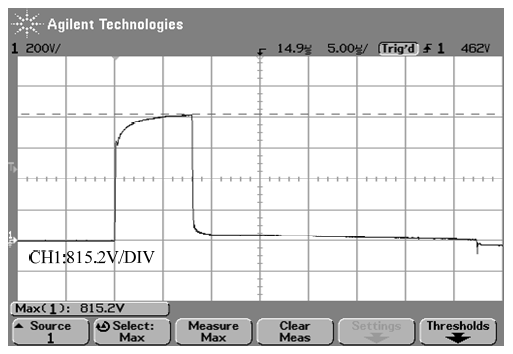
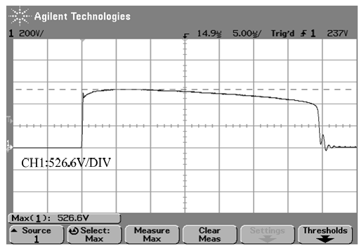
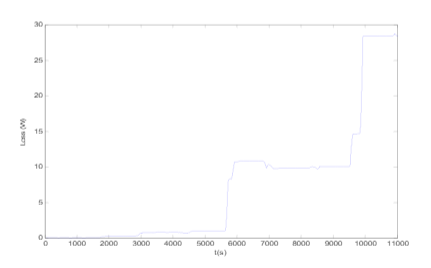
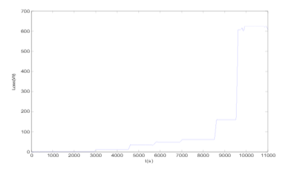
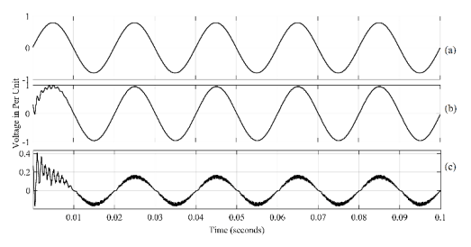
As an example, in Fig. 1 and 2 show graphs of active powers directed from the network to the load (P+) and from the load to the network (P-) at the point of transmission of electrical energy under the power supply contract


The figures show the moment of failure of the asynchronous motor (AM) of the mill of the processing plant, which was discussed above. A device for measuring power quality indicators “Resurs” [57] measured active powers. Graph in Fig. 2 shows that the active power supplied from the load to the network is zero.
It is necessary to develop an economic mechanism for managing the power quality, taking into account the capabilities of modern instruments for measuring indicators of the power quality and a methodology for determining the contribution of the distorting consumer to the distortion of the power quality.
4.6 Technical means to ensure the power quality
The concept of a smart power grid proposes 22 technical devices for normalizing the power quality in electrical networks [38]. The devices are divided into four groups depending on the method of connection to the electrical network: transverse, longitudinal, longitudinal-transverse devices, devices for combining electrical power systems and filters. Of the devices presented in the concept, a small number are used in electrical networks. The most commonly used of them are capacitor banks, controlled shunt reactors with magnetization, and passive harmonic filters. Currently, new effective technical means are being used and developed to comprehensively solve problems of electrical energy quality. Among them are active filter-balancing devices of the shunt type (transverse) and the serial type (longitudinal) [56]. They generate reactive power to reduce voltage sags, make the voltage symmetrical, and filter harmonics in a dynamic mode when the harmonics of the distortion source change rapidly. Modified magnetization-controlled shunt reactors are presented in [57]. They do not have a negative impact on the quality of electrical energy, unlike previously produced and used magnetization controlled shunt reactors. A pilot project of a converter device is presented in [58]. It is an active filter for installation in electrical networks of 10-220 kV in order to reduce asymmetry and non-sinusoidality of currents and voltages, stabilize voltage, reduce dips and voltage fluctuations. To solve problems with the power quality using special technical means, it is necessary to create and use standard devices of various capacities that compensate for the asymmetry and non-sinusoidality of currents and voltages in electrical networks of all voltages.
4.7 Periodic control and monitoring of power quality indicators
Period control and monitoring of the power quality is carried out in accordance with the current GOST 33073– 2014 [59]. Periodic control includes certification and arbitration tests of electrical energy, inspection supervision of certified electrical energy, control during the implementation of state control and supervision of consumer complaints, implementation of the energy supply contract in terms of the power quality, etc. Periodic measurements of power quality indicators in electrical networks have the disadvantage that events that cause a decrease in the power quality occur not only during the measurements. Therefore, the creation of a system for continuous monitoring of power quality indicators in the Russian electric power system is an actual task. Information received from the system for monitoring power quality indicators can be used to solve the following problems:
• assessment of the current state of the power quality when checking the compliance of measured indicators with established requirements in regulatory documents, energy supply contracts, etc.;
• obtaining information about the power quality in case of consumer complaints;
• providing information on the power quality to consumers when they connect and taking it into account when concluding energy supply contracts;
• assessment of the impact of low power quality on the service life of electrical equipment of consumers and power grid companies, generating electrical equipment, power and energy losses in asymmetrical and nonsinusoidal modes;
• selection and development of measures and technical means to normalize the power quality;
• assessment of the impact of distributed generation and new types of consumer electrical equipment on the power quality;
• planning the development of electrical networks, possible changes in the network structure, connection of consumers;
• forecasting, using special software, the power quality in various operating modes of electrical distribution networks and power supply systems;
• obtaining information about trends in the electrical network and individual areas in the field of power quality.
With the help of information received from the power quality monitoring system, in addition to the listed problems, many others can be solved. It is difficult to confirm the connection between consumer damage and poor power quality if, at the time of disruption of the enterprise’s technological process, during equipment failure, or for a long time before that, measurements of power quality indicators were not carried out. Currently, there are electricity meters that, in addition to commercial metering of electrical energy, record indicators of its quality. Such meters must have an event log with the date and time of voltage deviation from the norm, no voltage or voltage below a specified threshold in each phase, recording the time of voltage loss and restoration, etc. It is necessary to formalize the need to install a system for commercial metering of electrical energy with control of all indicators of the power quality at the initiative of the consumer or the electric grid company.
5 Conclusion
In Russia, it is necessary to create a system for managing the power quality in smart power systems in order to provide the digital economy with the proper power quality. To create a full-fledged power quality management system, it is necessary, first of all, to develop a concept for power quality management, taking into account the positive experience of previous years.
The research was carried out under State Assignment Project (No. FWEU-2021-0001) of the Fundamental Research Program of Russian Federation 2021-2030.
References
1. “On approval of the list of goods subject to mandatory certification and the list of works and services subject to mandatory certification,” Decree of the Government of the Russian Federation No.1013 of August 13, 1997.(in Russian)
2. Product quality management. Basic concepts. Terms and Definitions. GOST 15467-79. Moscow: Standardinform, 2009. (in Russian)
3. N.A. Melnikov, “On the issue of the power quality,” Elektrichestvo, no. 5, pp. 1-6. 1968.
4. Electric Power. Standards for power quality indicators at its receivers connected to generalpurpose electrical networks. GOST 13109-67. Moscow: Publishing house of standards, 1985. (in Russian)
5. Electric power. Electromagnetic compatibility of technical means. Quality regulation of electric power in general-purpose electric power supply systems. GOST 32144–2013, Moscow: Standardinform, 2014. (in Russian)
6. A.K. Shidlovsky, A.K. Kuznetsov, Improving the power quality in electrical networks. Kyiv: Nauk. Dumka, 1985, 268 p. (in Russian)
7. J. Arrilaga, D. Bradley, P. Bodger, Power System Harmonics: Translated from the English, Moscow: Energoatomizdat, 1990, 320 p. (in Russian)
8. I.I. Kartashev, E.N. Zuev, Power quality in power supply systems. Ways to control and ensure it. M: Izdatelstwo MEI, 2001, 120 p. (in Russian)
9. I.V. Zhezhelenko, Higher harmonics in power supply systems of industrial enterprises. M: Energoatomizdat, 2010, 375 p. (in Russian)
10. O.V. Zapanov, L.I. Kovernikova, “On the power quality supplied to joint stock company “Aleksandrovsky mine””. https://www.e3sconferences.org/artcles /e3sconf/abs/2020/69/e3sconf_energy12020_07012/e3sconf_energy212020_07012.html.
11. L.I. Kovernikova, V.V. Sudnova, R.G. Shamonov et al., Power quality: current state, outstanding issues, and proposals to their solutions. Novosibirsk: Nauka, 2017, 219 p. (in Russian)
12. V.E. Vorotnitsky, Yu.I. Morzhin, “Digital transformation of the Russian energy sector is systemic task of the fourth industrial revolution”, Energiya Yedinoy seti, no. 6(42), pp. 12-21. 2018. (in Russian)
13. Putin: “The formation of a digital economy is a matter of national security of the Russian Federation.” https://tass.ru/ekonomika/438941114. (in Russian)
14. “On approval of the Digital Economy of the Russian Federation program,” Government Order of the Russian Federation No. 1632-q of July 28, 2017. (in Russian)
15. Government Decree of the Russian Federation No.2425 of December 23, 2021. (in Russian)
16. Decision of the State Duma Committee on Energy No. 3.25-5/22 of April 6, 2022. Letter to the General Director of PJSC “Rosseti” A.V. Ryumin No. C70A-4/25 of February 15, 2022. (in Russian)
17. “On Amendments to the Federal Law “On Electric Power Industry” and Certain Legislative Acts of the Russian Federation”, Federal Law No. 174-FL. (in Russian)
18. “On Electric Power Industry”, Federal Law of the Russian Federation No. 35-FL of January 1, 2023. (in Russian)
19. L.N. Dobrusin, “Investments in the Russian electric power industry and a program to increase their efficiency”, in Proceedings of the VI All-Russian Energy Forum “Russian Fuel and Energy Complex in the 21-st Century”, 1-4 April 2008, Moscow. Final materials. (in Russian)
20. “On Electric Power Industry,” Federal Law of the Russian Federation No. 35-FL of March 26, 2003. (in Russian)
21. E.A. Mankin, “Eddy current losses in transformer windings with non-sinusoidal current.” Elektrichestvo, no. 12, pp. 48-52. 1955. (in Russian)
22. A.I. Tserazov, N.I. Yakimenko, “Information materials No. 70. Study of the influence of voltage asymmetry and non-sinusoidality on the operation of asynchronous motors”, Moscow: Gosenergoizdat, 1963, 120 p. (in Russian)
23. Electric Power. Requirements for the power quality in general purpose electrical networks. GOST 13109-87. Moscow: Publishing house of standards, 1988. (in Russian)
24. Electric Power. Electromagnetic compatibility of technical equipment. Standards for the power quality in general-purpose electrical networks. GOST 13109-97. Moscow: Standartinform, 1998. (in Russian)
25. “On the rules for certification of electrical equipment”, Resolution of the State Standard of the Russian Federation No. 36 of July 16, 1999. (in Russian)
26. “On introducing changes and additions to the Nomenclature of products and services (works), in respect of which the legislative acts of the Russian Federation provide for their mandatory certification,” Resolution of the State Standard of the Russian Federation No. 74 of August 14, 2001. (in Russian)
27. “Rules for connecting consumers to a general purpose network according to the conditions for influencing the quality of electricity,” Promyshlennaya energetika, no. 8, pp. 45-48. 1991. (in Russian)
28. “Rules for applying discounts and surcharges to tariffs for the quality of electricity,” Promyshlennaya energetika, no. 8, pp. 49-51. 1991. (in Russian)
29. “Tariffs for electric and thermal energy”, Price list No. 09-01. 1991. (in Russian)
30. Forensic electrical examination in case No. A78- 1996/03-С1-26/48 of the Arbitration Court of the Chita Region. (in Russian)
31. Civil Code of the Russian Federation of October 21, No. 14-FL. 1994. (Of July 3, 2016). (in Russian)
32. “On the Protection of Consumer Rights,” Federal Law of the Russian Federation of 02/07/1992 No.2300–1. (Of 07/03/2016). (in Russian)
33. “Methodology for determining the source (direction to the source) of distortions in power quality parameters/approved,” Deputy Chairman of the Board – Chief Engineer of JSC FGC UES Dikim V.P., of November 20, 2014. Included in the Federal Information Fund for Ensuring the Uniformity of Measurements under No. FR.1.34.2015.20724. (in Russian)
34. G. M. Mustafa, S.I. Gusev, “Experience in using active filter-compensating devices of shunt and serial type in electrical networks,” in Proc. of the International Scientific and Practical Conference “Electric Energy Quality Management”, Moscow, 2016, pp. 67-77. (in Russian)
35. A.I. Nenakhov, S.I. Gamazin, “Application of a low-power StatCom device in a system with an asymmetric load,” Promyshlennaya energetika, no.1, pp. 30-36. 2017. (in Russian)
36. G.M. Mustafa, S.I. Gusev, “Features of the use of modular multi-level converters for normalizing voltage quality indicators of the electrical network,” Elektroenergiya. Peredacha i raspredeleniye, no. 4(49), pp. 58-65. 2018. (in Russian)
37. E.V. Ilyashenko, Yu.V. Kolyuzhko, “Measuring instruments for monitoring and analyzing the quality of electrical energy,” in Proc. of the International Scientific and Practical Conference “Electric Energy Quality Management”, Moscow, 2016, pp. 134-143. (in Russian)
38. “Report on the agreement “Development of the Concept of an intelligent electric power system with an active-adaptive network” Agreement No. I-11-11/10,” Open Joint Stock Company “STC Electric Power Industry”, Moscow, 2011. (in Russian)
39. R. Hartungi, L. Jiang, “Investigation of power quality in health care facility”, in Proc. of the International Conference on Renewable Energies and Power Quality, Granada, Spain, 23-25 March, 2010.
40. I.V. Zhezhelenko, Yu. L. Saenko, T. K. Baranenko, “Selected issues of non-sinusoidal modes in electrical networks of enterprises,” Moscow: Energoatomizdat, 2007. 297 p. (in Russian)
41. A. Novitskiy, S. Schlegel, D. Westermann, “Estimation of Power Losses caused by Supraharmonics,” Energy Systems Research, vol. 6, no. 4, pp. 28-36. 2020.
42. S.P. Gladkikh, L.I. Kovernikova, A.V. Kostin et al., “Higher harmonics in connection nodes of traction substations (on the example of the East Siberian Railway)”, Irkutsk: ISEM SB RAS, 2002. 59 p. (in Russian)
43. G. R. Bossio, C. H. De Angelo, Donolo P. D. et al., “Effects of voltage unbalance on IM power, torque and vibrations”, In Proc. of the 2009 IEEE International Symposium on Diagnostics for Electric Machines, Power Electronics and Drives, Cargese, France, 2009.
44. Mechanical vibration ‒ Evaluation of machine vibration by measurements on non-rotating parts. Part I. General guidelines, ISO 10816-1:1995, International Standards Organization. 1995.
45. “Economic Framework for Power Quality,” Technical Brochure CIGRE, no. 467. 2011.
46. “In Glavgosenergonadzor of the Russian Federation,” Promyshlennaya energetika, no. 6, p. (in Russian)
47. “Regulations on state energy supervision in the Russian Federation,” Promyshlennaya energetika, no. 6, pp. 50-52. 1999. (in Russian)
48. “On the functioning of retail electricity markets, complete and (or) partial restrictions on the consumption of electrical energy,” Decree of the Government of the Russian Federation No. 442 of May 4, 2012. (in Russian)
49. “A state of emergency was introduced in the Mogochinsky district due to the failure of 17 engines and a pump in boiler houses”, URL: https://www.rosteplo.ru/ news/2017/12/12/1513024429-rejim-chs-vveli-v-mogochinskomrajone-iz-za-sboya-17 01.03.2022). (in Russian)
50. “On Technical Regulation,” Federal Law No. 184- FL of December 27, 2002. (in Russian)
51. “On Technical Regulation,” Federal Law No. 184- FL of December 23, 2021. (in Russian)
52. “Electromagnetic Compatibility,” Technical Regulations of the Customs Union TRTS 020/2011, Approved by decision of the Customs Union Commission No. 879 of December 9, 2011. (in Russian)
53. R.G. Shamonov, “Assessment of the influence of banks of static capacitors on the higher harmonic components of voltage in main electrical networks,” Energiya yedinoy set, no. 2 (19), pp. 22-29. 2015.
54. “In Glavgosenergonadzor of the USSR Ministry of Energy,” Promyshlennaya energetika, no. 11, p. 52. 1990.
55. “Measuring instruments,” Research and production association “Energotekhnika,” https://www.entp.ru/.(in Russian)
56. G.M. Mustafa, S.I. Gusev, A.M. Ershov et al., “Calculation of the power of an active filterbalancing device for normalizing the voltage on the buses of the 220 kV Skovorodino substation”, Elektricheskiye stantsii, no. 3, pp. 46-53. 2015. (in Russian)
57. A.M. Bryantsev, M.A. Bryantsev, M.A. Makarova, “Modified series of controlled shunt reactors and reactive power sources,” Elektroenergiya. Peredacha i raspredeleniye, no. 4 (49), pp. 94-100. 2018. (in Russian)
58. R.G. Shamonov, N.A. Alekseev, A.M. Matinyan, A.V. Antonov, “Experience and prospects for using a high-voltage active filter of the MPU series to improve the power quality,” Elektroenergiya. Peredacha i raspredeleniye, no. 2 (65), pp. 76-82. 2021. (in Russian)
59. Electric Energy. Electromagnetic compatibility of technical equipment. Control and monitoring of the power quality in general purpose power supply systems. GOST 33073-2014, Moscow: Standardinform, 2014(in Russian)
Source & Publisher Item Identifier: E3S Web Conf. Volume 461, 2023Rudenko International Conference “Methodological Problems in Reliability Study of Large Energy Systems“ (RSES 2023). https://doi.org/10.1051/e3sconf/202346101046