An Application of Facility Location Problem for Electricity Supply Cost Minimization at the Stage of Preliminary High Voltage Network Development Planning

Published by Piotr KAPLER, Warsaw University of Technology, Faculty of Electrical Engineering, Power Engineering Institute


Abstract. The article deals with minimizing the costs of electricity supply at the preliminary network planning stage. It presents selected information on costs in power engineering. The facility location problem and Mixed-Integer Linear Programming has been also described. A computational example of the application of this method is presented to solve the problem of minimizing the costs of electricity supply between high voltage / 110 kV power stations and 110 kV urban stations

Streszczenie. Artykuł dotyczy minimalizacji kosztów dostaw energii elektrycznej na etapie wstępnego planowania sieci. Przedstawiono w nim wybrane informacje dotyczące kosztów w elektroenergetyce. Opisano zagadnienie lokalizacji obiektów oraz metodę optymalizacji mieszanej całkowitoliczbowej liniowej. Zaprezentowano przykład obliczeniowy zastosowania tych metod do rozwiązania problemu zminimalizowania kosztów dostaw energii elektrycznej pomiędzy stacjami NN / 110 kV a stacjami miejskimi 110 kV. (Zastosowanie problemu lokalizacji obiektów do minimalizacji kosztów dostaw energii elektrycznej na etapie wstępnego planowania rozwoju sieci wysokiego napięcia).

Keywords: costs of electricity, costs minimizing, network development planning, mixed integer linear programming
Słowa kluczowe: koszty energii elektrycznej, minimalizacja kosztów, planowanie rozwoju sieci, optymalizacja mieszana.

Introduction

Electric Power System (EPS) consists of many interconnected elements whose purpose is the generation, transmission, distribution and usage of electricity. Simultaneously, it is a very important and strategic element of any area. Therefore, it is necessary that the decisions concerning power system taken at each stage of its design, operation or development, are optimal and reasonable. Thanks to this approach it should be possible to rationally manage energy sources, good operation of components as well as sustainable use of electricity by consumers both now and in the future.

Due to its complexity and large scale electric power system is a challenge for many optimization processes. Optimization tasks in this case can be both linear and nonlinear and have a large computational dimension. They are also accompanied by a number of different constraints, that must be maintained in order to model the correct operation of the power system. Often, the variables involved in the optimization process can be either integer or non-integer. Also some problems are NP-hard type. Optimization is proposed in each of the power system sectors: from generation to end consumers of electricity. Moreover, optimization may apply to both planned and already existing power infrastructure. Usually time horizon of optimization can be middle (2-5 years) or long term (10-20 years). The network planning process itself sometime takes into account the conditions of risk [1], uncertainty [2] or a probabilistic approach [3]. Factors encouraging the development are: an increase in power demand, the location of a new generation sources, access to fuels or increasing reliability of supplies [4].

This article is devoted to the minimization of electricity supply costs by application of facility location problem. Described situation occurs at the stage of preliminary high voltage (HV) network planning with usage of mixed integer linear optimization. The initial part of article presents selected issues about costs in power engineering. Also a description of the optimization method used is provided. The calculation part of article presents an example of minimizing the costs of electricity supply between potentially planned high voltage / 110 kV power stations and 110 kV urban stations. The final part of the article contains a summary and conclusions.

Selected issues concerning the costs of electricity supply

The operation of the power system is based on continuous coverage of the variable power demand of end users. Electricity, by its nature, cannot be stored easily and cheaply at present. At the same time, its production and transmission are associated with significant costs. These premises encourage rational management of electricity.

The supply of electricity is possible by building an appropriate infrastructure consisting of lines and power stations. The financial outlays for these investments are very large. In addition, it is also necessary to earn money on the provision of transmission services and collect funds for the ongoing operation and renovation works. In the future, investments in further network development may be required. Money can be obtained due to the difference between the total revenues that arose from the sale of goods or services and the total costs that had to be incurred in producing those goods and services.

In the case of power lines, expenditure on their construction is related with the length of the planned line, land charges and the use of specific technical solutions (for example types of poles or wires). It is estimated that the financial expenditure on the construction of a cable line is a multiple of 4 to 14 times the expenditure on the construction of an overhead line with the same rated voltage and length [5]. The operating costs result from the need to conduct qualified service work. Modifying the connections later on is cheaper and easier for overhead lines than for cable lines.

For power stations, investment outlays are related to the area where station is to be located, with the equipment used (for example circuit breakers or switch disconnectors) and the type of transformers. Operating costs will depend on the station layout used.

In addition, the transmission of electricity is accompanied by energy losses that must be paid for. Their values will depend on the length of the connections. They can be divided into load losses and idle losses.

Various methods are used in the electricity sector to determine fees for the provision of transmission services. The most popular include: the postage stamp method, the contract path method, the MW-mile method or method of tracing power flows. Each of the above methods give different outcomes as a result of the adopted assumptions and simplifications in their operation. The mentioned methods can be divided according to the way costs are treated. There are embedded cost methods and marginal cost methods. The first subgroup includes the postage stamp, contract paths and MW-mile methods. The second one is power flow tracing. Embedded costs deal with the power system as a whole and usage costs are borne by all users [6]. The marginal cost methods determine the value of the unit price to cover variable costs.

Linear mixed integer optimization and facility location problem

Linear programming has been used to solve optimization problems for many years. It is a special case of mathematical programming. Increased interest in this subject occurred at the turn of the 1950s and 1960s. Despite the fact that it is not new issue, nowadays it sill has a great application due to the development of computers and the application of possibilities for modern technical problems.

The idea behind this tool is to build a mathematical model that best reflects the characteristics of a real object as much as possible. Such a model is a record in the form of appropriate mathematical equations. The solution of the equations is the answer to the given decision problem. This approach helps making the final decision because building a mathematical model is cheap, simple and safe and does not require manipulating real objects.

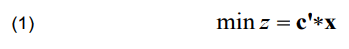
In general, the linear programming problem can be defined in matrix form as (1):

.

subject to conditions (2) and (3):

.

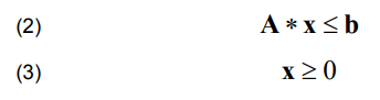
where: z – objective function, c’ – matrix of objective function coefficients, A – matrix of limiting conditions coefficients, x – matrix of variables (unknowns), b – matrix of limiting values of the right side of the inequality (2). Formula (3) is a non-negative condition.

Each model consists of three basic elements. These are: the objective function (also known as the criterion function), decision variables and set of limiting conditions. The objective function is describing the goal to be pursued in the optimization task. This function is being minimized or maximized. It has a linear form. Decision variables are a description of resources related to the modelled issue. They are non-negative. The constraint conditions reflect the limits in the modelled process. They are described as inequalities with left sides containing linear functions.

Despite the simplicity of implementation, linear programming in its classic form is not always suitable for solving most optimization problems. It may turn out that in the description of the problem it will be necessary to include binary values (0 or 1) representing for example the existence or non-existence of a given object depending on certain conditions. In order to solve such problems, linear mixed integer optimization (MILP – Mixed Integer Linear Programming) is used. This approach applies if some (but not all) of the variables are binary.

In general, MILP problems can be defined identically using formula (1) and (2). However, condition (3) is replaced with condition (4).

.

where some variables are integer type and the rest are binary (0 or 1).

This type of approach is particularly useful for solving optimization problems in the power engineering industry, for example: the switching on or off generation units [7], designing distribution networks [8] or multistage planning of the development of the transmission network [9].

Optimization problems solved with the use of MILP must meet the following simplifying assumption: the share of each of the variables in the objective function is proportional to this variable and, at the same time, independent of the values of other variables in the task. Additionally, the values of constraints and decision variables must be known before performing optimization calculations. Sometimes, however, these values are not known exactly because they were derived from a rough estimate. Their influence on the optimization result can be obtained by applying a sensitivity analysis.

The facility location problem is well-known in optimization theory. In general, it deals with selecting the best locations of facilities that will cover the given customers demand while minimizing the costs of transportation. The input data are: set of candidate facility locations F = {1,…,m}, set of customers C = {1,…,n}, a cost function and a distance function. Moreover, the cost function may contain not only information about the cost of delivery but also the cost of opening a given facility. The result of calculation is the assignment of all customers to all opened facilities. Optimization models with facility locational problem can also be extended with additional constraints like: availability of fuels, raw materials or cost of land. Further description of this problem can be found in [10,11].

There are many variations of this task. In presented solution the mentioned problem has a MILP form – opening (or not) a new facility is a binary value. The objective is to minimize the total costs which can be divided to costs of opening new high voltage / 110 kV power station and costs of supply (which are proportional to the distance between power station and customers).

Formulation of the optimization problem

The optimization problem concerned the issue of minimizing the cost of electricity supply at the stage of preliminary high voltage network planning. The solution was obtained with an application of facility locational problem for power system planning. In the presented case facilities were 4 potentially planned high voltage / 110 kV power stations while customers were 9 urban 110 kV power stations. Every customer station can be theoretically supplied by each of planned HV / 110 kV station. The aim of the task was to find such connections between power stations so that the cost of electricity supply was minimal while simultaneously covering the required demand for active power.

All 110 kV power stations were located at different distances from supplying stations so the delivery cost was also dissimilar. It was assumed that the transmission of electricity to all customers can take place without violating any technical limitations like voltage drops or long-term current carrying capacity. Furthermore, it was also assumed that the total active power in supply stations was equal to the demand of consumers (Case 1) or supply exceeds that demand (Case 2).

The objective function (minimizing the cost of electricity supply) was defined as follows (5):

.

subject to conditions (6), (7) and (8):

.

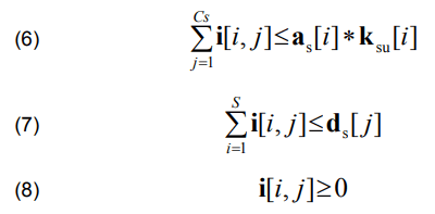
where: C – objective function constituting the cost of electricity supply subject to minimization, S – total number of power stations i, bs – the price of the building of the i-th power station, ksu – binary value related to the use of the station (0 – station not used, 1 – station used), es – cost of i-th station exploatation, c – delivery cost matrix for each station-customer pair, i – the amount of electricity transmitted from the i-th station to j-th customer, kl – power loss cost, Cs – total number of customers j, as – active power available at the station, ds – demand for active power at given customer.

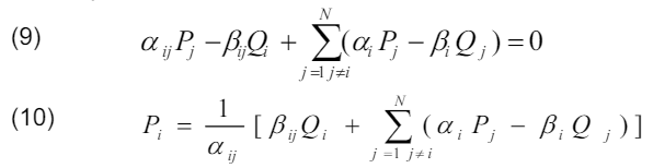
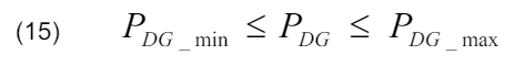
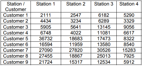
In the objective function (5) it was taken into account that the cost of electricity supply from the HV / 110 kV to 110 kV stations will depend on the distance, active power demand, fixed cost related to the operation of a given high voltage station and the value of the charge for transmission power losses. Table 1 contains the values of the cost of delivery parameters for all potential station-customer pairs. They were created by applying the MW-mile method in which the delivery cost is defined by the formula (9) [12]:

.

where: Cdi – cost Energy supply, Pji – active power flow in the j-th line for the i-th transaction, Dj – length of the j-th line, Rj – required unit renewal value per line length.

The unit value of the renovation was 1.5% of the power line construction cost. The average price of building 1 km of high voltage lines was determined on the basis of data from [13]. The cost of construction of the high voltage / 110 kV power station was estimated at PLN 150 million (around 37 million euros). The costs of maintenance and repairs of each power station were assumed for 4% of capital expenditure [14].

Table 1. Energy supply costs form the MW-mile method, all values in PLN.

.

At the preliminary planning stage, it was assumed that all possible station-to-customer connections were taken into account. Some of these connections may later be rejected in further stages of network planning if it turns out that they are less optimal than others.

Solving the optimization problem

The task of minimizing the cost of electricity supply was solved in two cases. Case 1 assumed that the sum of active power in all power stations was equal to the sum of active power demand for all customers. In case 2, it was assumed that the planned total active power in all stations is greater than the customers demand. Table 3 presents the active powers in the stations for case 1 and case 2.

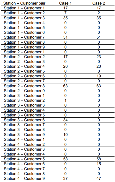
The solution of the problem was presented in the form station-customer pairs, for which, as a result of optimization calculations, active power values were allocated to cover the total demand at the customer (110 kV station) with the lowest possible cost of delivering and meeting additional conditions – expressed by the equations (6)-(8).

Table 4 shows binary values (1 or 0) corresponding to the necessity to build (or not) a given high voltage / 110 kV station in each of the cases. Table 5 contains the final summary of the results for both analysed cases. Where the connection of a given station with customer would not be optimal, the value of 0 appears. It is worth noting that connections with the value of 0 can be both in case 1 and case 2. This means that regardless of the values of available active power the given connection is not optimal.

Table 2. Demanded active powers, in MW

.

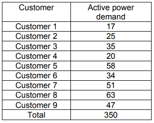
Table 3. Active powers in high voltage power stations, in MW

.

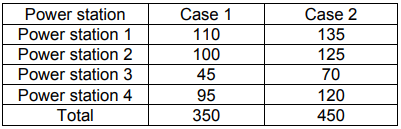
Based on the presented optimization results, the following values of the objective function (electricity supply cost) were obtained: for case 1 – PLN 650 244 922, and for case 2 – PLN 493 955 302. The result for case 2 is smaller because the calculations show that building of high voltage station 3 is redundant. Consequently, each Station 3 – customer pair has a 0 value in Table 5. Hence the result for case 2 is taken as an optimal for the considered planning problem.

Table 4. Binary values corresponding to the need to build a given power station in each case.

.

Table 5. Results of the optimization task solution, active powers in MW.

.
Summary and conclusions

The article presents an optimization task consisting in minimizing the costs of electricity supply at the stage of preliminary high voltage network planning. According to the conducted research, case 2 turned out to be more favourable than case 1. The objective function for case 2 is around 75% of the cost for case 1. However, the difference in cost values is PLN 156 289 620. This is more than the assumed construction price of the one high voltage / 110 kV power station.

The presented example relates to the situation when it is planned to transmit power form high voltage / 110 kV power stations to 110 kV stations located in a large urban agglomeration. In this case, the knowledge from the above analysis may be useful in further planning stages of the power network development for example, to the construction of load flow and short-circuit network models. The mentioned method may also be effective for making decisions concerning medium and low voltage network development. Due to the use of binary values, it can also be used to decide on the closing of existing power stations.

The results of the performed analysis depend on the input data used. It is necessary to choose the method by which the charges for transmitting electricity will be calculated. It is assumed that the price criteria used in the planning process should also take into account the problem of renewal of elements [15]. The second important factor is knowing the prices for the construction of the power line. The value of this price will strongly depend on many factors like type of line (overhead or cable) or the way it is located.

The advantage of the presented methodology using the mixed-integer approach is its efficiency, scalability and simplicity. The model used is universal and after introducing minor modifications it can be adopted to other optimization problems in the power engineering industry. Even if the obtained solution does not turn out to be fully satisfactory, it may constitute a starting point for the search of a new result. The disadvantage of an inaccurately conducted analysis may be both underinvestment and overinvestment in the transmission network [16]. Also, using the mixed-integer approach may be difficult due to possibly large number of binary (0,1) decision values.

When solving the problems of planning the power network development it is necessary to conduct multivariant analyses of various possible technical solutions. On this basis, it will be possible to further conclude whether it is worth implementing the intended investment or not. In the process of building decision models it is convenient to use, for example, linear programming. In addition, knowledge about the necessary investment outlays is also essential.

REFERENCES

[1] Marzecki J., Planowanie rozwoju miejskich Rozdzielczych Punktów Zasilających (RPZ) w warunkach ryzyka, Przegląd Elektrotechniczny, 90 (2014), nr. 2, 234-237
[2] Marzecki J., Planowanie rozwoju miejskich stacji 110 kV/SN w warunkach niepewności, Przegląd Elektrotechniczny, 96 (2020), nr. 1, 23-26
[3] Kubek P., Przygrodzki M., Wybrane aspekty wykorzystania elementów probabilistycznych w planowaniu rozwoju sieci przesyłowej, Przegląd Elektrotechniczny, 94 (2018), nr. 12, 108-111
[4] Gonen T., Electrical Power Transmission System Engineering: Analysis and Design, CRC Press, 2014
[5] Underground vs. Overhead: Power Line Installation-Cost Comparison and Mitigation, https://www.powergrid.com/2013/02/01/underground-vs-overhead-power – line-installation-cost-comparison/#gref (accessed 24.04.2020)
[6] Saganek D., Koszty wykorzystania elementów SEE w powiązaniu ze stanami pracy SEE – właściwości podejścia opartego na idei wpływu, Przegląd Elektrotechniczny, 91 (2015), nr. 5, 159-165
[7] Kamiński J., Kaszyński P., Mirowski T., Szurlej A., Krótkoterminowy matematyczny model systemu wytwarzania energii elektrycznej dla warunków Polski, Rynek Energii, czerwiec 2014
[8] Turkay B., Distribution System Planning Using Mixed Integer Programming, Elektrik, 6 (1998), nr. 1, 37-48
[9] Zhang H., Vittal V., Heydt G. T., J. Quintero, A mixed-integer linear programming approach for multi-stage securityconstrained transmission expansion planning, IEEE Transactions on Power Systems, 27 (2012), nr. 2, 1125-1133
[10] Dantzig G. B., Linear Programming and Extensions, Princeton University Press, Princeton, New Jersey, 1991
[11] E. Castillo, A. J. Conejo, P. Pedregal, R. Garcia, N. Alguacil, Building and Solving Mathematical Programming Models in Engineering and Science, John Willey and Sons, 2002
[12] Song Y-H. (edit), Modern Optimisation Techniques in Power Systems, Springer Science + Business Media, 1999
[13] Ciupak S., Linie WN na słupach kratowych vs linie WN na słupach rurowych, Konferencja Naukowo-Techniczna Elektroenergetyczne linie napowietrzne i kablowe wysokich i najwyższych napięć, Wisła 18-19.10.2017
[14] E. Dyka, I. Mróz-Radłowska, Ekonomia w Energetyce. Wybrane zagadnienia, Politechnika Łódzka, Łódź 2014.
[15] Einhorn M., Siddiqi R. (edit), Electricity Transmission Pricing and Technology, Kluwer Academic Publishers, 1996
[16] Dołęga W. Aspekty rynkowe planowania rozwoju sieciowej infrastruktury elektroenergetycznej, Energetyka, 8 (2015)


Author: Piotr Kapler, Ph. D., Warsaw University of Technology, Faculty of Electrical Engineering, Power Engineering Institute, Koszykowa 75, 00-662 Warsaw, Poland. E-mail: piotr.kapler@ien.pw.edu.pl


Source & Publisher Item Identifier: PRZEGLĄD ELEKTROTECHNICZNY, ISSN 0033-2097, R. 96 NR 11/2020. doi:10.15199/48.2020.11.35

Methods of Calculating Solar Insolation for the Assessment of Energy Efficiency of Solar Power Plants

Published by Sergey CHIZHMA, Artyom ZAKHAROV, Immanuel Kant Baltic Federal University (Kaliningrad, Russia)


Abstract. The authors explore a number of methods of calculating insolation on a tilted arbitrarily oriented surface and choose the most efficient one for conducting the performance and efficiency analysis of solar power plants. The validity of the method is tested using the statistical data of the Kaliningrad region. The authors describe an algorithm for calculating insolation in the Matlab software programme, based on the following data: the position of the Sun, the average monthly climatic characteristics of the region, beam, scattered and reflected insolation as well as the proportion of these types of insolation on a tilted surface. The authors validate the results of their calculations by comparing them with statistical averages.

Streszczenie. Analizowano metody obliczania nasłonecznienia dowolnie pochylonej powierzchni. Walidację metody przeprowadzono na podstawie danych statystycznych regionu Kaliningrad. Obliczenia przeprowadzono na podstawie znajomości pozycji słońca, średniej miesięćżnej informacji klimatycznej, średniego nasłonecznienia. (Metoda obliczania nasłonecznienia dowolnie pochylonej powierzchni)

Keywords: alternative energy, insolation, energy, efficiency
Słowa kluczowe: energia nasłonecznienia, ogniwa fotowoltaiczne

Introduction

The construction of solar power plants requires assessment of energy potential of a chosen territory. In most cases, design solutions for solar power plants are based on long-term average measurements that include the average daily solar energy (kWh/(m2·day)), average daily wind speed (m/s), etc. The main sources of data used for estimating solar energy potential are insolation maps, NASA data [1] and the data provided by the World Radiation Data Centre [2] for actinometric stations of the World Meteorological Organization (WMO) network, etc. [3]. There is an extensive body of literature on hybrid energy solutions, types of renewable energy, their classification and composition. Reviews on different types of solar energy solutions are presented in [4-6].

There is a need for a more accurate assessment of the efficiency of solar power plants. This task requires more objective data reflecting the impact of a number of factors associated with the location and the position of solar panels, annual variations in the length of daylight hours, and cloudiness. In our research, we propose to move from the average energy parameters, which are, in essence, quantitative characteristics of insolation, to instantaneous values of insolation incident on a tilted surface in order to determine daily fluctuations of insolation. We also propose a method for assessing the efficiency and performance of solar power plants based on this approach.

The aim of the research

The main aim of our research is to test a method of calculating insolation for obtaining more accurate data on its instantaneous values based on geographical location and average climatic parameters. We hold that the obtained data can be used for modeling and assessing the energy generation performance of solar power plants [7] and the optimization of their control algorithms. We tested the proposed method using input data for the Kaliningrad region and validated the results of the calculation.

To achieve the aim, we analysed a number of calculation methods, which are based on the algorithm for determining the position of the Sun for different geographic locations and seasons (Section 1). Various computational methods for estimating insolation on the Earth’s surface are described in the works of Liu and Jordan [8-10], KolaresPereira and Rabl [11], and Gueymard [12-13].

We have chosen one calculation method that meets the objectives of our research (See Section 2) and used it for the determination of solar insolation on a tilted surface (Section 3). The selected model has been applied to obtain insolation data for the Kaliningrad region for one year. Power plants based on renewable energy sources can be simulated with obtained data, as shown in [14-15]. The results of our calculations have been verified (Section 4).

1. Methods of calculating the position of the Sun

The existing methods of estimating instantaneous values of insolation require the analysis of the position of the Sun above the Earth’s surface [16]. The annual change in solar activity is associated with two main factors: the annual change in the solar declination angle δs, and the annual change in the distance between the Earth and the Sun. The axial tilt of the Earth’s orbit is 23.45°. Thus, the declination angle δs (solar declination) varies in the range from -23.45° to 23.45° during the year and can be calculated using the Cooper formula [17]:

.

where n is the ordinal number of the day in the year.

To simplify the calculation of the position of the Sun above the Earth’s surface, the Earth is considered as a stationary object. Figure 1 shows that the observation point is assumed as the origin of the coordinates. In this system, the Sun is a moving object and rotates around the centre of the Earth with an angular velocity of 15° per hour. The zenith point (or local noon) is taken as the starting point for the revolution of the Sun. The value characterizing the movement of the Sun around the Earth is called the solar hour angle hS. It is calculated using the formula:

.

The two values, the angular height of the Sun α and the azimuth angle of the Sun αs are used to calculate the spherical coordinates of the position of the Sun above the Earth’s surface:

.

where L is the geographical latitude.

Fig.1. Determination of the solar hour angle hs, the angle of declination of the Sun δs, the angular height of the Sun α and the azimuth angle αs

Solar radiation on the Earth’s surface depends on the changes in the distance between the Earth and the Sun during the year: on the day of the winter solstice, December 21, it is 1,471·1011 m and on the day of the summer solstice, June 21, it constitutes 1,521·1011 m. This variability is a function of the elliptical shape of the Earth’s orbit, which is taken into account when translating the so-called solar time (the zenith time is 12.00) into local time using the following formula:

.

where ET is the equation of time, taking into account the variability of the Earth’s rotation speed around the Sun, lst is the standard time meridian, llocal is the local longitude. ET is determined using the formula given below:

.
2. The analysis of the methods of calculating insolation on the Earth’s surface

The calculation of insolation on the surface of the Earth is a difficult task since it requires taking into account a variety of factors. There are many empirical or semiempirical approaches to the problem within which a number of simplifying assumptions are made. Each of the assumptions is based on the calculation of three main types of insolation on the Earth’s surface: beam insolation (Ib.c), scattered or diffused insolation (Id.c) and reflected insolation (Ir.c):

.

To account for the absorbing effect of clouds, a monthly clearness index (KT) is introduced. It can be calculated using the formula:

.

where Hh [kWh/(m2·day)] is the monthly average daily radiation on a horizontal surface, and Ho.h [kWh/(m2·day)] is the monthly average daily extraterrestrial radiation [16].

This index was first proposed in the works of Liu and Jordan [8–10]. The method of calculating radiation, considered in the framework of this approach, is applied to monthly average values. In our research, we propose to calculate the instantaneous values of insolation during the day. There are a number of methods that allow researchers to move from average values of solar radiation to instantaneous ones:

• the Kolares-Pereira and Rabla method developed in 1979 (CPR-method) [11],

• the Kolares-Pereira and Rabla method, modified by Gyeumard in 1986 (CPRG-method) [12],

• the Daily Integration (DI) Model, developed by Gyeumard in 2000 [13].

Based on the data presented by Christian A. Gueymard in [13], the daily integration (DI) model is more accurate than other methods listed above. Therefore, in this paper, the calculation of insolation is done using this method. The daily integration model is based on the calculation of rd and rt, which change during daylight hours. They demonstrate the dependence of instantaneous diffused insolation and instantaneous insolation on a horizontal surface on the total daily scattered insolation and total daily insolation on a horizontal surface, respectively.

The coefficient rd is defined as follows:

.

where hss is the solar light angle corresponding to the sunset, hereinafter expressed in radians. The method of calculating hss is described in [16].

According to the daily integration model, the rt coefficient is calculated as follows:

.

where the absorption of radiation in the atmosphere is taken into account using the ratio a2/a1:

.

The coefficients A(hss) and B(hss) are defined as follows:

.

Missing values for the calculation are defined as indicated below:

.
.

Thus, the instantaneous value of insolation on the horizontal surface Ih [Wh/m2] and the instantaneous value of diffused insolation Id [Wh/m2] can be calculated in the following way:

.

Then, beam insolation on a horizontal surface, Id.h [Wh/m2] is calculated according to the formula:

.
3. Calculation of solar radiation on a tilted surface

The values of insolation obtained using the daily integration method are to be converted into insolation values for solar panels oriented and tilted in a particular way. The position of solar panels is set at the following angles (Fig. 2): the tilt of the solar panels β and the azimuth angle of the solar panels αw. The incident angle of sunlight on the surface of the solar panels i is determined as follows:

.

Using simple transformations, we determine the fraction of beam insolation on the tilted surface Ib.c:

.
Fig.2. Calculation of insolation on a tilted surface

Scattered insolation (Id.c) on the surface of solar panels is estimated as follows:

.

Reflected insolation (Ir.c) is calculated using the formula:

.

where ρ = 0.2 for the surface not covered with snow, and 0.8 for the snow-covered surface.

Thus, the insolation on the tilted surface is determined as follows:

.
4. Calculation of insolation for the Kaliningrad region

The calculation method described in the sections above was used in the MATLAB software programme for obtaining the annual insolation data for the Kaliningrad region (54°43′N, 20°30′E). The algorithm (Fig. 3) is based on NASA resource data [1], where Hh is average monthly total radiation on a horizontal surface per day, Hd is average monthly total scattered radiation, and KT is monthly clearness index:

Fig.3. Block diagram of the algorithm for calculating insolation

Other input data for the algorithm are the latitude, the longitude of the chosen terrain, the start and finish dates of the formation of the calculated insolation values, as well as parameters characterising the location of the solar panels. The algorithm performs the calculation of the ordinal numbers of the days in the year (taking into account leap years) for which the calculation of solar insolation is done. NASA data are monthly averaged, so before starting the calculation, the change in monthly average indicators is interpolated, and their values for each day are determined. The variable, linearly dependent on time, is the hour angle of the Sun hs, for which every minute values are calculated. After all the data have been formed, the MATLAB software programme calculates the total insolation on a tilted surface, thus forming the data array Ic.

Figure 4 shows the calculated insolation on the surface of a solar panel having a 30° tilt angle on December 21, June 21, and March 1.

The reliability of the calculation method and the data obtained have been assessed. To perform the assessment we analysed the calculated total monthly radiation incident on a horizontal as well as on a tilted surface. The results are shown in Fig. 5, where Hh.calcu is the calculated average monthly total radiation, Hh is the average monthly total radiation according to NASA [1], and Hc is the monthly average total radiation.

Fig.4. Insolation on the tilted surface

Fig.5. Estimation of the data reliability

The graph shows that the margin of error of the proposed method is minimal. It allows us to use the obtained data for the performance and efficiency analysis of solar power plants.

Conclusions

In our research, a number of methods for calculating instantaneous values of insolation have been analysed. The methods are based on the calculation of the coordinates of the position of the Sun (the angular height and the azimuth angle), as well as the average climatic parameters of the season.

Our analysis of the calculation methods has shown that the daily integration model (DI) is the most effective one. On the basis of this model, we proposed an algorithm for calculating insolation using the MATLAB software programme. This allowed us to determine instantaneous values of insolation for a wide variety of temporal and geographic conditions. The algorithm can be used to form an array of objective data on the instantaneous values of insolation on the tilted surface of solar panels, as a combination of beam, diffused and reflected insolation.

We validated the obtained data and identified the margin of error of the proposed method, which turned out to be insignificant. The proposed method of calculation can be used to simulate the operation of power plants working on renewable energy sources, evaluate their efficiency and to conduct further research on optimizing control algorithms for autonomous solar power plants.

REFERENCES

[1] https://power.larc.nasa.gov/data-access-viewer/.
[2] World Radiation Data Centre. Available at: http://wrdc.mgo.rssi.ru/ (accessed 14 March 2017)
[3] Popel’ O.S., Frid S.E., Kiseleva S.V., Kolomiec Ju.G., Lisickaja N.V. Klimaticheskie dannye dlja vozobnovljaemoj jenergetiki Rossii (Baza klimaticheskih dannyh). M.: Izd-vo MFTI. 2012
[4] Chauhan A., Saini R.P. A review on Integrated Renewable Energy System based power generation for stand alone applications: Configurations, storage options, sizing methodologies and control // Renewable and Sustainable Energy Reviews. – 2014. –V. 38. – Р. 99–120.
[5] Shivarama K.K., Sathish K.K. A review on hybrid renewable energy systems // Renewable and Sustainable Energy Reviews. – 2015. – V. 52. – Р. 907–916.
[6] Badwawi R.A., Abusara M., Mallick T. A Review of Hybrid Solar PV and Wind Energy System // Smart Science. – 2015. – V. 3 (3). – Р. 127–138.
[7] Obuhov S.G., Plotnikov I.A. Imitacionnaja model’ rezhimov raboty avtonomnoj fotojelektricheskoj stancii s uchetom real’nyh uslovij jekspluatacii. Izvestija Tomskogo politehnicheskogo universiteta. Inzhiniring georesursov. 2017. T. 328. № 6. 38–51
[8] Liu, B.Y.H., R.C. Jordan. 1960. The interrelationship and characteristic distribution of direct, diffuse and total solar radiation. Sol. Energy 4: 1–19.
[9] Liu, B.Y.H., R.C. Jordan. 1961a. Daily insolation on surfaces titled toward the equator. Trans. ASHRAE 67: 526–541.
[10] Liu, B.Y.H., R.C. Jordan. 1961b. Daily insolation on surface tilted toward the equator. Trans. ASHRAE 3(10): 53–59
[11] Collares-Pereira M, Rabl A. The average distribution of solar radiation: Correlations between diffuse and hemispherical and between daily and hourly insolation values. Solar Energy 1979; 22: 155-164.
[12] Gueymard C. Monthly averages of the daily effective optical air mass and solar related angles for horizontal or inclined surfaces. J Solar Energy Eng Trans ASME, 1986
[13] Gueymard C. “Prediction and Performance Assessment of Mean Hourly Global Radiation” Solar Energy, Vol. 68, No. 3, 2000, pp. 285-303. doi:10.1016/S0038-092X(99)00070-5
[14] Mirosław Mazur , Janusz Partyka , Tomasz Marcewicz. Analysis of the use of a hybrid power system of renewable wind and photovoltaic energy in residential buildings. PRZEGLĄD ELEKTROTECHNICZNY, ISSN 0033-2097, R. 92 NR 8/2016. 113-116.
[15] Kazimierz Buczek, Wiesława Malska, Sebastian Penar. Use of PSIM software for modelling a small solar power station. PRZEGLĄD ELEKTROTECHNICZNY, 08/2011 Page no. 42.
[16] D. Yogi Goswami. Principles of solar engineering. Third Edition. CRC Press. Taylor & Francis Group 2015.
[17] Duffie J.A., Beckman W.A. Solar Engineering of Thermal Processes. Hoboken, New Jersey, John Wiley & Sons, Inc., 2013.


Authors: Prof. Sergey N. Chizhma, the Institute of Physics, Mathematics and Information Technologies, Immanuel Kant Baltic Federal University, Kaliningrad Russia. E-mail: chisn@yandex.ru, Artyom Zakharov, PhD student, the Institute of Physics, Mathematics and Information Technologies, Immanuel Kant Baltic Federal University, Kaliningrad, Russia. E-mail: AIZakharov@kantiana.ru.


Source & Publisher Item Identifier: PRZEGLĄD ELEKTROTECHNICZNY, ISSN 0033-2097, R. 96 NR 11/2020. doi:10.15199/48.2020.11.26

The Problem of Determining the Coefficient of Flicker in Accordance to Normative Regulations

Published by Marta BĄTKIEWICZ-PANTUŁA, Wrocław University of Science and Technology, Institute of Electrical Power Engineering


Abstract. The article presents an analysis of the selected parameter of the power quality. The analysis was done in accordance with the applicable normative regulations. The results presented in the article were made on the basis of actual measurements of the electricity quality parameters. Two different objects were analyzed: a group of industrial receivers and a network cooperating with renewable energy sources.

Streszczenie. W artykule zaprezentowano analizę wybranego parametru jakości energii elektrycznej. Analiza została przeprowadzona zgodnie z obowiązującymi przepisami normatywnymi. Zamieszczone w artykule wyniki zostały wykonane na podstawie rzeczywistych pomiarów parametrów jakości energii elektrycznej. Analizie zostały poddane dwa różne obiekty jakim była grupa odbiorników przemysłowych oraz sieć współpracująca z odnawialnymi źródłami energii. (Problematyka wyznaczania współczynnika migotania światła zgodnie z aktualnymi przepisami normatywnymi).

Keywords: flicker, regulation of the minister, updating of the EN 50160 standard, industrial customer of electricity, renewable power plants
Słowa kluczowe: współczynnik migotania światła, rozporządzenie ministra, aktualizacja normy EN 50160, odbiorcy przemysłowi, energia odnawialna

Introduction

The phenomenon of voltage fluctuations appeared with the beginning of the existence of electricity distribution systems. More attention to this phenomenon have been given with the increase in the number of receivers and their installed capacity. In order to better understand the disorders and the effects they cause, in many countries they started to fight this problem through numerous researches aiming at a thorough understanding of the phenomenon itself and its measuring assessment.

Until recently, voltage fluctuations in the power supply or the load terminals, were described by specifying the maximum size of the change in value of the effective voltage.

The energy of voltage fluctuations and the spectral density of power of voltage fluctuations were also used, (also called the energy spectrum of voltage fluctuations). The duration of the fluctuations and the interval between changes in voltage was also included in the assessments.

Parameters according to which the quality of the supply voltage should be assessed are included in the Regulation of the Minister of Economy [1], which is a valid legal act and in relation to recipients supplied from low, medium and high voltage public power networks in PN-EN 50160 [2,3]. An important group of documents in this area is the multipart PN-EN 61000-xx standard with the general title “Electromagnetic compatibility” [4,5], which defines the acceptable levels of environmental and operational interference that are required to ensure the correct operation of electrical devices connected to the network and defines the measurement methods and methods for determining these disturbances.

The phenomenon of the flicker is a voltage changes that have the character of regular fluctuations, which occurs for a long time, which can cause changes in luminous flux generated by electric light sources. This phenomenon has an adverse effect on the comfort and concentration of people working in such conditions, and its measure is the flickering index, the permissible levels are specified in the Regulation [1] and the Standard [2]. The indicator of flicker is determined for all voltage levels in the power network [2], both for the highest voltages (connection groups I and II), as well as medium and low voltage (connection groups III – V).

The determination of acceptable levels of the flicker indicator also in the case of medium and high voltages, i.e. those at which the light source is not directly supplied, indicates the high importance of this parameter and the possibility of propagating interference at various voltage levels across the entire distribution network. Connecting the devices of significant powers to the network, which may cause the phenomenon of flickering of light (welding machines, often switched on and off motors, arc furnaces) should be preceded by an analysis aimed at checking whether the flickering effect caused by this device will fall within the permissible range [2]. In the analysis of this important parameters are: the nominal power of the device, the short-circuit power of the network and the nature of voltage changes caused by the operation of the device.

Measurement of voltage fluctuations is carried out in order to assess the compliance of existing levels of the phenomenon with the relevant standards, as well as to determine the emission level of a given receiver and compare it with the limit values in the standards. There are two basic methods of measurement:

• based on a quantitative evaluation of the phenomenon based on a temporary change in the effective value or voltage envelope,

• based on indirect measurement – measurement of the phenomenon of flickering of light which is a direct result of voltage fluctuations.

The phenomenon of flickering of light, known in the world literature under the name “flicker”, is one of the parameters for assessing the power quality. It depends on the instability of the perception of human vision, but this instability is caused by a light stimulus whose luminance or spectral distribution is subject to changes in time due to fluctuations in the voltage supplying the light source.

The rules for calculating the flicker ratio are specified in the standard [6]. This factor consists of two elements:

• short-term flicker factor Pst, determined for the observation time of 10 minutes, according to the dependence:

.

in which P0.1 percentiles; P1; P3; P10 and P50 are flicker levels exceeded by 0.1; 1; 3; 10 and 50% of the observation time. The index s in the above dependence indicates that should used the smoothed values.

• long-term flicker factor Plt determined for the observation time of 2 hours and calculated using the next 12 Pst factors for this observation time, according to the formula:

.

The primary document in the process of assessing the power quality is the Regulation of the Minister of Economy of 4 May 2007 on detailed conditions for the operation of the power system with the last update in 2008. The subordinate document is the PN-EN 50160 standard: Voltage characteristics of electricity supplied by public electricity networks which until now has been updated three times, i.e. in 2008, 2010 and 2015.

The Regulation of the Minister of Economy and the PNEN 50160 standard to be updated in 2010 were in line with the power quality requirements for the assessment.

Table I presents the comparison of the requirements for the parameter of the power quality which is the flicker. The list has been presented for nn and SN networks.

Table 1. Permissible limits of the flicker factor

.

The first column indicates the requirements set by the Regulation of the Minister of Economy in the second and third column requirements to be met according to PN-EN 50160 in 2010 and from 2015.

Analysis Of Measurements

The basis for assessing the power supply conditions is the Regulation of the Minister of Economy of 4 May 2007. on detailed conditions of the power system operation. The article presents the assessment of the parameters of power quality in accordance with the Regulation of the Minister [1] and the PN-EN 50160 [2] standard and its update [3]. According to the normative assumptions, a representative period was selected which was a normalized time basis for the presented runs and determined power quality indicators. In a representative measurement period if disturbances were noted, i.e. dips, power interruptions, according to [3], no such measurement results should be considered. The article uses only those measurement results that were considered significant from the point of view of this work.

Figure 1 shows the general schematic diagram of the measurement system. The main element of the measurement system was the Fluke 1760 recorder.

Fig.1. General schematic diagram of the measuring system

The actual measurements presented in the article have been divided into two groups. In the first group of industrial receivers supplied from the power grid was presented two examples of circuits, which are, the welding circuit, and installed arc furnace circuit. In the second group are the working with renewable sources medium voltage energy networks, also present in two cases, with the network hydroelectric plant and a wind power plant.

The first of the discussed cases are groups of industrial receivers supplied from power grid.

Figure 2 can be seen the values of the long-term and short-term flicker indicators on the L1 phase, obtained during measurements for welding circuit. The full observation time of the recorded parameters was one week. In the representative measurement period, no disturbances were detected that would affect the analyzed process. The indicators that are calculated in accordance with the methods described in the standard [4] are shown on below waveforms.

Fig.2. Flicker on example of L1 phase: Short-term indicator Pst (thin); Plt long term indicator (bold)

It can be observed that for the analysed case, the power quality parameter does not exceed the permissible limits contained in the documents [1-3]. The value of the flicker indicator (long-term) is a maximum of 0.85 which is in accordance with the required ministerial regulation [1], standard [2] which refers to 95% of observation time and norm [3] for 100% of observation time. Permissible limits for the short-term coefficient were not specified in the Minister’s Regulation [1] and the Standard [2]. Coefficient Pst = 1.4 meets the requirements of the updated standard [3] despite exceeding the required value 1.2. The value was exceeded in less than 5% of cases, which corresponds to requirement 1.2 for 95% of the measurement data set.

The next analyzed case is presented in Figure 3. The recorded values of long-term and short-term flicker on the L1 phase example, were presented, they were collected during measurements for the circuit where arc furnace was installed. The complete observation time of the recorded parameters was four days. In the representative measurement period, no disturbances were detected that would affect the analyzed process. The presented waveforms refer to flicker indicators was calculated in accordance with the methods described in the standard [4].

Fig.3. Flicker on example of L1 phase: Short-term indicator Pst (thin); Plt long term indicator (bold)

It can be observed that for the analysed case, the power quality parameter does not exceed the permissible limits contained in the documents [1-3]. The value of the long-term flicker factor is a maximum of 0.13 which is in accordance with the required ministerial regulation [1], standard [2] which refers to 95% of observation time and norm [3] for 100% of observation time. Permissible limits for the short-term flicker factor were not specified in the Minister’s Regulation [1] and the Standard [2]. The Pst = 0.16 coefficient meets the requirements of the updated standard [3].

The second of the discussed cases are medium voltage network working with renewable energy sources The first case where renewable sources are working of with medium voltage network is presented in Figure 4. Presented are the collected values of long-term and short-term flickers on the example of phase L1, obtained during measurements for a hydroelectric power plant. The full observation time of the recorded parameters was one week. In the representative measurement period, no disturbances were detected that would affect the analyzed process. The presented waveforms refer to the flicker factors calculated in accord with the methods from the standard [4].

It can be observed that for the analyzed case the power quality parameter exceeds the acceptable limits contained in the documents [1-3]. Value of the long-term flicker is a maximum of 1.8 which is in accordance with the required ministerial regulation [1], standard [2] which refers to 95% of observation time. Standard [3] requires fulfillment of the parameter for 100% observation time, so exceeding the permissible value of 1 to 1.8 results in failure to meet the acceptable limit. The coefficient of short-term flicker in accordance with the regulation of the minister [1] and the norm [2] does not have admissible limits. The Pst = 4.0 coefficient meets the requirements of the updated standard [3] despite exceeding the required value 1.2. The value was exceeded in less than 5% of cases, which corresponds to requirement 1.2 for 95% of the measurement data set. In the analyzed case, a solution should be considered to improve the power quality parameters.

Fig.4. Flicker on example of L1 phase: Short-term indicator Pst (thin); Plt long term indicator (bold)

The next case is presented in Figure 5. Presented are the collected values of long-term and short-term flicker factors on the example of phase L1, obtained during measurements of a wind farm. The full observation time of the recorded parameters was one week. In the representative measurement period, no disturbances were detected that would affect the analyzed process. The presented waveforms refer to the flicker factors determined in accord with the methods from the standard [4].

Fig.5. Flicker on example of L1 phase: Short-term indicator Pst (thin); Plt long term indicator (bold)

It can be observed that for the analysed case, the power quality parameter does not exceed the permissible limits contained in the documents [1-3]. The value of the long-term flicker indicator is a maximum of 0.8 which is in accordance with the required ministerial regulation [1], standard [2] which refers to 95% of observation time and norm [3] for 100% of observation time. Permissible limits for the short-term coefficient were not specified in the Minister’s Regulation [1] and the Standard [2]. The Pst = 1.8 coefficient meets the requirements of the updated standard [3] despite exceeding the required value 1.2. The value was exceeded in less than 5% of cases, which corresponds to requirement 1.2 for 95% of the measurement data set.

Summary

The tightening of the normative provisions that followed the introduction of the PN-EN 50160 [3] standard was aimed at improving the parameters of the power quality.

The change in the power quality parameters concerned the setting of a limit for the short-term flicker factor, which until the update was undefined. At the same time, the requirements set for the long-term factor flickers were tightened. Additional information that introduces the update of the standard is defining the normal working time. The concept of normal working time refers to the state of the systems without any disturbance. If during the analyzed measurement period there are events, they should be excluded from further analysis.

Analyzing the examples presented in the article, it can be concluded that the tightening of the limits permitted for the flicker factors did not significantly affect the power quality for individual or industrial consumers. The tightening of limits has affected the network cooperating with renewable sources. Renewable power plants are characterized by variability of work which is associated with a large irregularity of parameters. The tightening of allowable limits has had a particularly strong effect on rapidly variable and irregular burdens. It can be concluded that for customers where device start-ups will occur frequently or there will be large parameter changes, the introduction of a limit for the short-term flicker factor will result in non-compliance with the normative requirements.

The problem with tightening the permissible limits for power quality parameters occurs when according to the superior document, i.e. the minister’s regulation [1], the power quality parameters meet the requirements and subordinate document, i.e. the PN-EN 50160 [3] standard, the power quality parameters already conditions do not meet. Until the update in 2015, such a problem did not exist because the subordinate document defined the same limits as in the parent document.

REFERENCES

[1] Regulation of the Minister of Economy dated. May 4, 2007 on detailed conditions of functioning of the power system (Journal of Laws of 29 May 2007, item 623).
[2] EN 50160:2010. Voltage characteristics of electricity supplied by public electricity networks.
[3] EN 50160:2015. Voltage characteristics of electricity supplied by public electricity networks.
[4] PN-EN 61000-4-15: 2011 Electromagnetic Compatibility (EMC) – Test and Measurement Methods – Flicker Meter – Functional and design specifications.
[5] PN-EN 61000-4-30:2015 Electromagnetic compatibility (EMC)-Part 4-30: Testing and measurement techniques – Power quality measurement methods
[6] PN-EN 61000-3-3:2013, Electromagnetic compatibility – Permissible levels – Limiting voltage fluctuations and flicker caused by receivers with rated current < or = 16 A in low voltage supply networks.
[7] Guide to Quality of Electric Supply for Industrial Installations, Part 5, Flicker and Voltage Fluctuations, “Power Quality” Working Group WG2, 2000
[8] A.Klajn, M.Bątkiwicz-Pantuła, Application Note – Standard EN50160: Voltage characteristics of electricity supplied by public electricity network,. European Copper Institute, 2013.


Authors: dr inż. Marta Bątkiewicz-Pantuła, Wrocław University of Science and Technology, Faculty of Electrical Engineering, Institute of Electrical Power Engineering, 27 Wybrzeże Wyspiańskiego St, 50-370 Wrocław, Poland. E-mail: marta.batkiewiczpantula@pwr.edu.pl


Source & Publisher Item Identifier: PRZEGLĄD ELEKTROTECHNICZNY, ISSN 0033-2097, R. 96 NR 1/2020. doi:10.15199/48.2020.01.13

Analysis of Transient Waveforms in a Power System at Asymmetrical Short-Circuits

Published by Piotr PRUSKI, Stefan PASZEK, Silesian University of Technology


Abstract. In the paper, there is presented the analysis of disturbance waveforms of a synchronous generator operating in a single-machine power system consisting of a generating unit connected by a high-voltage power line to a bus. There are considered disturbances in the form of symmetrical and asymmetrical short-circuits in different places of the transmission line. The current-voltage equations of the power line and the bus are written for phase components, which allows for easy modeling of various asymmetries.

Streszczenie. W artykule analizowano przebiegi zakłóceniowe generatora synchronicznego pracującego w jednomaszynowym systemie elektroenergetycznym składającym się z zespołu wytwórczego, połączonego linią energetyczną wysokiego napięcia z siecią sztywną. Uwzględniono zakłócenia w postaci zwarć symetrycznych i niesymetrycznych w różnych miejscach linii przesyłowej. Równania prądowo-napięciowe linii energetycznej i sieci sztywnej zapisano dla składowych fazowych, co pozwala na łatwe modelowanie różnych asymetrii. (Analiza przebiegów nieustalonych w systemie elektroenergetycznym przy zwarciach niesymetrycznych).

Keywords: power system; generating unit; asymmetrical short-circuits; transient states.
Słowa kluczowe: system elektroenergetyczny, zespół wytwórczy, zwarcia niesymetryczne, stany nieustalone.

Introduction

Short-circuits are the most common and severe kind of faults occurring in the power system (PS). Most often they are asymmetrical short-circuits. Symmetrical short-circuits rarely occur in practice as compared with asymmetrical ones (only a few percent of the total number of cases). Over half of short-circuits in overhead high voltage lines are transient short circuits [1]. Asymmetrical PS operating conditions cause many unfavorable phenomena, i.a. in synchronous generators. It causes the necessity to limit the duration of such operating conditions [2, 3, 4].

Due to the difficulty in modeling asymmetrical operating conditions, symmetrical short-circuits are mainly analyzed in simulation investigations. Most specialized programs for the analysis of PS transient states allow for simulation of only symmetrical operating conditions. Therefore, it is reasonable to conduct research aimed at simulating the disturbance waveforms of selected quantities for different asymmetries occurring in PS. For this purpose, commonly used models of generating unit elements can be used, but some modifications should be introduced in them.

The analysis of asymmetrical PS operating states, including short-circuits, may help e.g. in better selection of power protection settings [5, 6]. The values and waveforms of different PS quantities may vary considerably depending on the type of the occurring asymmetry. Only effectively functioning protections can reduce the negative effects of disturbances, which allows reducing the consequences of faults occurring in PS.

The aim of the paper is a comparison and a harmonic analysis of the disturbance waveforms of selected quantities for different short-circuits with earth and clear to earth in a single-machine PS, consisting of a generating unit, a high-voltage transmission line and a bus. There was also analyzed the influence of the distance between the short-circuit location and the influence of including or neglecting effects of particular elements of the generating unit model.

Model of the analyzed PS

As a part of the conducted research, a mathematical model of the PS was developed in the Matlab-Simulink environment. In this model, using Configurable Subsystem blocks, it is possible to conveniently configure a specific model of the generating unit by selecting models of its individual elements.

In the carried out calculations, there were used: the GENROU [7, 8] synchronous generator model with subtransient asymmetry X”dX”q [3, 6, 9, 10] as well as the models of the static excitation system operating in the Polish Power System [7], the IEEEG1 steam turbine [7, 8] and the PSS3B system stabilizer [7].

When analyzing asymmetrical operating conditions of the PS, it is convenient to express the equations of stator currents and voltages, transmission line and bus with use of phase quantities. The Park transformation is used to relate the quantities in the d, q, 0 coordinate system to those in the phase A, B, C coordinate system [2, 3, 6, 7, 9, 10, 11, 12].

In the investigations, there were analyzed various asymmetries occurring in the transmission line. Fig. 1 shows a diagram of the analyzed PS for short-circuits with earth and clear to earth. On its basis, the model of the power line and the bus was developed.

Fig.1. Diagram of the analyzed PS for short-circuits with earth (a) and clear of earth (b)

Symbols in the figure: ij – generator stator currents (phase quantities, j = A, B, C), vj – generator stator voltages, vbj – bus voltages, Zj – complex impedances of the transmission line, Zsj, Zbj – impedance of the j-th phase line fragments during the short-circuit, Ifd – generator field current, vd – voltage between the neutral points of the generator and the bus, ibj – bus currents, vs – voltage at the short-circuit location, WG – generator neutral point ground switch.

This schematic diagram for short-circuits with earth (Fig. 1a) applies to both normal PS operation and a short circuit. In order to model a earth short-circuit in selected phases, one should assume zero voltages of the bus vbj in these phases and change the impedances of the line proportionally:

.

where: l – relative distance of the short-circuit location in the transmission line from the generating unit, in relation to the length of the whole line.

In connection with the assumed omission of transformation voltages [2, 6, 12], on the basis of Fig. 1, there were determined the algebraic relations between currents and voltages in the generator stator and transmission line equations. For healthy phases:

.

for phases short-circuited to ground:

.

where: φj – phase angles of the particular transmission line impedances, f = 50 Hz. From (2a) and (2b) three equations were derived. In addition, for the system with ungrounded generator neutral point (open switch WG in Fig. 1a):

.

Using the generator stator axial voltages (output signals of the generator model and the generating unit model) and the axial voltages of the bus, it is possible to determine the phase voltages by the inverse Park transformation. Hence, from the system of equations (2), one can calculate four unknows: three phase currents and possibly the voltage vd at successive time instants. This is implemented in the developed model in the Matlab-Simulink environment. Using the formulas for the generator phase currents and Park transformation, the generator axial currents, being the input signals of the generator model and the generating unit model, were determined.

Fig. 1b presents a diagram for a 2-phase short-circuit clear of earth. The following equations determine algebraic relations between currents and voltages for this fault:

.

where: Δtj, Δtbj – time delays of the current waveforms, defined as in (2a); other symbols as in formulas (2).

From the system of equations (3) one can calculate seven quantities: five phase currents and voltages: vs and vd. The thus determined PS model is complete and allows for carrying out simulation calculations.

Exemplary calculations

In the calculations presented, the generator worked with grounded neutral point (closed switch WG in Fig. 1a, voltage vd = 0) in order to check an effect of the zero axial components of stator currents and voltages on the phase waveforms. In real high-voltage power systems, generators work usually with isolated neutral points.

In the first case, simulation calculations were performed for 3-phase short-circuits and 2-phase short-circuits with earth (in phases A and B) with a duration time equal to 0.15 s. There were analyzed short-circuits at different distances l from the generating unit for the generating unit with and without a PSS. It was assumed that in the steady state before the short-circuit, the generator was loaded with active power P0 = 0.5 p.u. and reactive power Q0 = 0.2 p.u.

Figures 2 and 3 show the waveforms (in relative units p.u. [4, 6, 7, 10, 11, 12]) of the angular speed deviation of the generator rotor Δω and the generator instantaneous power P in the analyzed cases, for different relative distance l from the generating unit.

In the second case, there were analyzed long-lasting short-circuits: 1-phase with earth (in phase A), 2-phase clear of earth (in phases A and B) and 3-phase, at the distance l = 1% from the generating unit. In this case also breaks in the non short-circuited phases were assumed. In the steady state before the short-circuit the following load was assumed: P0 = 0.1 p.u. and Q0 = 0.05 p.u. The influence of the excitation system, the turbine and the PSS was neglected in this case.

Fig. 4 show the waveforms of stator current iA (in relative units) for the analyzed fault types.

Tab. 1 presents the harmonic amplitude distributions of the current in phase A, the voltage in phase C and the field current in the steady state of the short-circuit. The higher harmonics percentage values are given in relation to the first harmonic for the stator quantities, and in relation to the constant component for the generator field current. The reference values in relative units (p.u.) are given in brackets.

Conclusions

The calculations made allowed formulating the following conclusions:

• The use of the transmission line and bus model for the phase components of currents and voltages in the developed PS model allows for easy modeling of various symmetrical and asymmetrical short-circuits with earth and clear of earth, as well as breaks in individual phases of the transmission line.

• The disturbance waveforms of the analyzed quantities in the case of a two-phase short circuit with earth differ significantly from those for a three-phase short-circuit. During the two-phase short-circuit, the waveforms of the instantaneous power of the generator have components with relatively high frequencies (in comparison with the frequency of electromechanical swings). Such components do not occur under symmetrical operating conditions, including the three-phase short-circuit. After the short circuit, in each of the analyzed cases, the generating unit returns to symmetrical operation and only low-frequency components associated with electromechanical phenomena occur. After the three-phase short-circuit, the amplitudes of the deviations from the steady values of the waveforms, especially of the angular speed, are much larger than those after the two-phase short-circuit.

Fig.2. Waveforms of the generator rotor angular speed deviation Δω for the system without the PSS: for two-phase short-circuit with earth (a), for three-phase short-circuit (b); for the system with the PSS: for two-phase short-circuit with earth (c), for three-phase short-circuit (d)

Fig.3. Waveforms of the generator instantaneous power P for the system without the PSS: for two-phase short-circuit with earth (a), for three-phase short-circuit (b); for the system with the PSS: for two-phase short-circuit with earth (c), for three-phase short-circuit (d)

Table 1. Harmonic amplitudes of the analyzed quantities in the steady state

.
Fig.4. Currents in phase A: a) envelopes, b) enlargement of one period in the steady state

• The use of the PSS with appropriately selected settings allowed for significant increase in the damping of electromechanical swings in the PS. As a result, the angular stability of the PS improved significantly and the time needed to return to the steady state after the disturbance was shortened. In the analyzed cases, the PSS did not have a significant influence on the amplitudes of the deviations from the steady values of the waveforms during and immediately after the short-circuit.

• In the cases under consideration, the influence of the distance between the short-circuit location and the generating unit on the waveforms of the analyzed quantities is large only during the short-circuit duration. After the short-circuit, it is significant only in the case of the three-phase short-circuit for the system without the PSS, and in other cases it is negligible.

• The maximal amplitude of the generator long-lasting short-circuit current in the steady state occurs at the 1- phase short-circuit. The current amplitude in the steady state at the 2-phase short-circuit is higher than that at the 3- phase short-circuit. It complies with the synchronous machine theory [3, 13].

• In the cases of the asymmetrical short-circuits, odd higher harmonics with significant amplitudes occur in the steady state waveforms of the short-circuit current and the stator voltage on the non short-circuited phase. The generator field current in steady state includes a constant component and even higher harmonics. The harmonics distributions in the short-circuit current and the non short-circuited phase voltage are similar for both types of asymmetrical short-circuits. Only the third harmonic of the voltage at the 1-phase short-circuit has a much lower amplitude. The harmonics distributions in the field current are similar for the both types of asymmetrical short-circuits.

• At the 3-phase symmetrical short-circuit, the stator current and voltage waveforms includes practically only the first harmonic, and in the field current waveform only the constant component occurs. The generator subtransient asymmetry does not cause the occurrence of higher harmonics in case of the machine symmetric operation. The presented power system model is also used in other investigations. They focus on various RL and XT-type synchronous generator models [7, 8] taking into account or neglecting the stator transformation voltages, with different input and output signals. A further extension of the model is planned.

REFERENCES

[1] Kacejko P., Machowski J, Zwarcia w systemach elektroenergetycznych [Short-circuits in power systems] (in Polish), WNT, Warszawa, 2009
[2] Concordia Ch., Synchronous Machines. Theory and Performance, John Wiley & Sons, Inc., New York, 1951
[3] Boldea I., Synchronous Generators, Taylor & Francis, 2015
[4] Pyrhonen J., Jokinen T., Hrabovcova V., Design of Rotating Electrical Machines, Wiley & Sons, Ltd, 2008
[5] Ungrad H., Winkler W., Wiszniewski A., Protection techniques in electrical energy systems, Mercel Dekker Inc., New York 1995
[6] Machowski J., Bialek J., Bumby J., Power System Dynamics. Stability and Control, John Wiley & Sons, Chichester-New York, 2008
[7] Paszek S., Berhausen S., Boboń A., Majka Ł., Nocoń A., Pasko M., Pruski P., Kraszewski T., Measurement estimation of dynamic parameters of synchronous generators and excitation systems working in the National Power System (in Polish), Monograph No. 504, Wydawnictwo Politechniki Śląskiej, Gliwice, 2013
[8] Boboń A., Paszek S., Pruski. P., Kraszewski T., Bojarska M., Computer-aided determining of parameters of generating unit models basing on measurement tests, Przegląd Elektrotechniczny, 5 (2011), pp. 17-21
[9] Berhausen S., Boboń A., Determination of high power synchronous generator subtransient reactances based on the waveforms for a steady state two-phase short-circuit, Applied Mathematics and Computation, 319 (2018), pp. 538–550
[10] Wang X., Song Y., Irving M., Modern Power Systems Analysis, Springer Boston, MA, 2008
[11] Krause P., Wasynczuk O., Sudhoff S., Pekarek S., Analysis of Electric Machinery and Drive Systems, third ed., Wiley-IEEE Press, 2013
[12] Gao J., Zhang L., Wang X., AC machine systems, Mathematical Model and Parameters, Analysis, and System Performance, Springer-Verlag, Berlin-Heidelberg, 2009
[13] Krause P.C., Analysis of electric machinery, McGraw-Hill, 1986


Authors: dr inż. Piotr Pruski, E-mail: Piotr.Pruski@polsl.pl, prof. dr hab. inż. Stefan Paszek, E-mail: Stefan.Paszek@polsl.pl, Politechnika Śląska, Wydział Elektryczny, Instytut Elektrotechniki i Informatyki, ul. Akademicka 10, 44-100 Gliwice.


Source & Publisher Item Identifier: PRZEGLĄD ELEKTROTECHNICZNY, ISSN 0033-2097, R. 96 NR 2/2020. doi:10.15199/48.2020.02.05

Arc Plasma Energy Evolvement in 60 kV Network Circuit Breakers

Published by Salah Belkhir1, Abderrahmane Ziani1, Hakim Azizi2, Hocine Moulai1,
University of Science and Technology Houari Boumediene, Algiers, Algeria (1), University Ziane Achour, Djelfa, Algeria (2) ORCID: 1. 0000-0002-5106-2821


Abstract. The evolvement of the electric and energetic properties of electric arcs at the poles opening of a circuit breaker (CB) is described by nonlinear mathematical models. Most of these models are dimensional types that do not describe the interaction between the arc and the network during the interruption phase. This paper is aimed at the determination of the energy necessary for the arc creation at the opening of a high-voltage circuit breaker with a black box model. The advantage of this model consists of its ability to link the intrinsic characteristics of the arc to the extern blowing (quenching) power. Moreover, it provides fast and stable solving without needing for spatial dimensions of the breaker. The model is applied to a line circuit breaker for which experimental results are available in the literature. Two phases of arc quenching evolvement are evidenced: Constant energy phase followed by a decreasing energy one. The Kema-based model is found to be more accurate for online plasma quenching analysis and the obtained results agree well with experimental ones where the heat energy represents the dominating part.

Streszczenie. Ewolucję właściwości elektrycznych i energetycznych łuków elektrycznych przy otwarciu biegunów wyłącznika opisują nieliniowe modele matematyczne. Większość z tych modeli to modele wymiarowe, które nie opisują interakcji między łukiem a siecią podczas fazy przerwania. Celem artykułu jest określenie energii niezbędnej do wytworzenia łuku przy otwarciu wyłącznika wysokonapięciowego z modelem czarnej skrzynki. Zaletą tego modelu jest możliwość powiązania wewnętrznych charakterystyk łuku z zewnętrzną mocą nadmuchu (gaszenia). Ponadto zapewnia szybkie i stabilne rozwiązywanie bez konieczności wymiarowania przestrzennego wyłącznika. Model stosuje się do wyłącznika liniowego, którego wyniki eksperymentalne są dostępne w literaturze. Wykazano dwie fazy rozwoju gaszenia łuku: faza stałej energii, po której następuje faza malejącej energii. Stwierdzono, że model oparty na Kema jest dokładniejszy do analizy hartowania plazmowego w trybie online, a uzyskane wyniki dobrze zgadzają się z wynikami eksperymentalnymi, w których dominującą część stanowi energia cieplna. (Ocena energii łuku plazmowego w wyłącznikach sieciowych 60 kV)

Keywords: High voltage, circuit breaker, energy, plasma quenching.
Słowa kluczowe: Wysokie napięcie, wyłącznik, energia, hartowanie plazmowe.

Introduction

High voltage circuit breakers (CB) are necessary switchgear for the protection of electrical networks. In both low and high voltage networks, there is a very large number of breaking techniques that use the electric arc as a way to evacuate energy [1-5]. Also, the low cut-off times of less than some milliseconds and the high energy released during the electric arc formation in high voltage circuit breakers make the measurements difficult to achieve and also expensive [6-8]. The development and manufacture of HV circuit breakers require a detailed knowledge of heat transfer mechanisms that evolve at the arc extinction [2, 9, 10]. Although these phenomena are important and of great interest, one notes that only few articles are devoted to.

To extinguish the electric arc appearing at the opening of a high voltage circuit breaker, all the electromagnetic energy stored by the network must be dissipated [1, 11, 12]. Following the high Joule energy released during the CB opening which can reach 30000 J [11, 13, 14], the arc can be cooled through a strong blow of a suitable gas.

In this paper, a power balance has been set up in order to model the energy needed for the creation of the arc during the extinction phase. A precise description of that energy is essential because it determines the dielectric recovery of the arc. The model has been implemented in the Simulink- Matlab environment to determine at first the arc voltage and conductance, and then to calculate the arc creation energies. The model takes into account the ionization time constant of the arc, its voltage, current and even the external blowing power.

Mechanisms of the electric arc formation

Thanks to a mechanical system and as a result of fault current occurrence the high voltage circuit breaker electrodes separate in a quenching chamber. However, after contacts separation, an arc appears and the current continues to flow. In the presence of a gas, this arc is associated to the corresponding plasma.

The filling gas is usually SF6, chosen for its excellent thermal and dielectric properties [11]. The electric arc occurs in the zone of high ionic and electronic density provided from the inter-contacts medium or metal vapors from the circuit breaker poles [2]. The junction zones that bridge the arc column to the contacts are at temperatures close to the melting point of the metal, hence the thermoionic emission is possible [15]. Thus, the electric arc consists of plasma composed of ionized gas and metal vapors.

The arc quenching Models found in the literature [14, 16-20] are always based on Maxwell’s equations, Ohm’s law and the conservation equations of mass and energy. Delalondre et al. [21] developed a two-dimensional code to simulate switching in high voltage circuit breakers. They obtain fields of temperature and potential close to experimental ones. Chevrier et al proposed in [22] a switching arc model in low voltage circuit breakers, while Lindmayer et al [23] have developed a three dimensional model for a low-voltage circuit breaker which predicts the arc movement as a function of temperature and pressure. In addition, Gonzalez [14] adapts a commercial code (Fluent) for thermal plasma behavior in low-voltage circuit breakers. Cassie and Mayr, Lowke et al [24] and Wang et al. [25] have modeled two-dimensional variations of temperature and conductance of quenching arcs in air and SF6. On the other hand, Schavemaker et al [18] and Guardado et al [19] show that a 0D model is sufficient to follow the evolution of arc voltage in high voltage circuit breakers.

Energy balance of the electric arc

The rich bibliography about energy transfer available in [26-33] shows that energy models are based on the conservation equations of mass and energy.

.

where ρ and H are respectively the density and enthalpy of the plasma, v its velocity, j the current density, B the magnetic field induction, Pray the power lost by radiation and T the thermodynamic temperature.

Experimental measurements have shown that the term (j Λ B) representing the induced current in the arc is often negligible [14], except for vacuum circuit breakers [34]. The appearance of the electric arc of current i(t) at the separation of the contacts creates an arc voltage U(t) that will determine a thermal elementary Joule energy dW during a time dt, thereby producing a very high temperature rise. The expression of this energy is given by:

.

The energy balance per time unit or the power balance reported to the arc in absence of magnetization is expressed by the following relationship:

.

Where Parc is the total electric power, PJ represents the Joule power provided to the arc which plays a role in the arc temperature rise, P is the cooling capacity due to the blowing of SF6, PC the power lost by thermal conduction and Pray the power dissipated by radiation.

The term PC can be expressed as a function of the arc temperature T and the temperature T0 of the external environment by the following relationship:

.

where, K is the thermal conductivity of the arc and r its radius.

Even if their dissipation assessment is necessary [35, 36], the terms Pray and PC are usually neglected in black box models calculations [18]. Thus, Pray and PC are estimated to 1% in [21]. Rachard et al [29] reported that the thermal energy dissipated by conduction has moderate influence on the power balance.

New energy model approach

The arc models can be classified into two groups: physical models based on hydrodynamic codes deducted from Navier-Stokes and black box models where the local properties are averaged and their governing equations do not make appear differential terms on the space variables. This is why they are called 0D models. These include the models of Mayr, Cassie and Kema [11, 13].

Also, to follow the energy Q of arc creation in a circuit breaker during its extinction phase, the following assumptions will be adopted. They have been used by several authors [11, 13, 37] in 0D models, namely:

– The arc column is cylindrical in shape.

– The resistivity is constant and its section decreases during extinction.

– The electric field within the arc is constant – The energy of arc creation is proportional to its base surface.

To establish a simple model governing the arc formation, one must assume that the conductance g is only expressed as a function of energy Q used for this arc formation.

.

Q represents macroscopically the plasma ionization energy [11, 13].

Thanks to a differential equation, we can also write that the difference between the electric power supplied by the network u i and the cooling power P injected by blowing is used to create the arc.

.

where P is the total cooling power provided to the arc, u the arc voltage, i the current through the arc and dt/dQ the power necessary for the arc creation. By expressing the differential of equation (5) as a function of time by multiplying and dividing by the same quantity dQ , we obtain:

.

Ohm’s law for a constant electric field E and a current i(t) crossing through an arc of cylindrical geometry and radius R gives for an electric resistivity ρ:

.

The conductance per unit length of a cylindrical arc can be expressed by:

.

where S is the surface of arc column. The arc section can be then deduced:

S= g x ρ

The surface of the arc assumed in the Cassie’s assumption [22] has been used to determine the energy Q necessary to create the arc:

.

One obtains then:

.

So, we have:

.

And by substituting the value of Cc by Q/S and the value of g by S/ρ, we obtain:

.

This equation can be replaced by the logarithmic expressions between Q and g:

.

Three 0D models (black box) are used to describe the evolution of the term Q through g. By using the Mayr equation, we obtain the following expression:

.

Where, P represents the blowing power in Watts and τ the deionization constant of the blowing gas (SF6).

Similarly, Q can be followed by Cassie equation given by the following expression:

.

where uc is the Cassie constant voltage. By using the Kema equation, one then obtains:

.

Where P is the external blowing power and P1 a regulation coefficient that is 0.9943. The consecutive arc column surface evolvement is depicted on figure1.

Presentation of the used Electrical network

The HV electrical network used for simulation of breaking arc is shown in Figure 2. Such approach is suitable to take into account external parameters of the CB including the topology of the network and the connected loads [38, 39]. The modelled CB has the same characteristics than that used by Schavemaker et al. [18], namely longitudinal impedance including a resistance and reactance per unit length of the line and two transverse admittances. This network is powered by an electromotive force e = 60 kV. The network characteristics are as follows:

Inductance L=3.5×10⁻³ H, Resistance R=30 Ω and Capacitance C=2.10-6 F. The frequency is set to 50 Hz. Figure 2 shows the Matlab Simulink synoptic diagram of the studied network. The simulations were performed thanks to the SIMpower SYSTEM tool.

Fig. 1. Arc extinction physical behaviour

Simulation

In this work, we focused on a typical HV SF6 circuit breaker used in substations and for which experimental results are available in the literature [13, 14, 16-19]. The simulation begins by initializing the arc parameters. The initial conductance g0 of the plasma is first fixed to104 S/m which corresponds to a conducting state. It will allow us to compare our results with those obtained by Schavemaker [18]. The initial energy Q0 is then set to 104 J.

Figure 2. Matlab Simulink synoptic diagram of the studied network
Figure 3. DEE block used to solve the Mayr Model

The circuit breaker opening time was set to 0.02 s. The blowing power of SF6 was simulated by the Step block of Simulink with a step equal to the opening time of the circuit breaker. The simulation time was fixed between 0 and 0.03 s to allow comparisons with experimental results available in the literature. Several solvers of differential equations have been tested to obtain the best convergence of the solution to finally choose the ode45/Matlab solver with a variable time step in order to satisfy a relative tolerance of 10-3.

Mayr, Cassie and Kema differential equations solving was made by the use of the Differential Equation Editor (DEE) block. The conductance was replaced by the variable x and the current by the expression u.exp(x). The solutions of the equations are generated in the DEE block as currents that are afterwards injected into the network. The steps followed to solve the Mayr model are presented below. Thus the differential equation was multiplied by the variable u(2) that has been introduced to control the opening time of the circuit breaker by providing a zero signal since the opening time is not reached.

.

By setting ln(g) = x , we obtain:

.

u(2)=0 for a time less than the breaker opening time.

u(2)=1 : For a time greater than or equal to the breaker opening time.

where g is the arc conductance, u(1) the arc voltage and i the arc current.

The output signal is a function of type y= exp(x(1)) x u(1) . To transform it into a usable current, a controlled current source is inserted at the output of the DEE. Figure 3 shows the adopted solving diagram in the Simulink environment.

Results and Interpretations

The variations of arc voltage in SF6 through the three models, namely Mayr, Cassie and Kema, for τ = 0.3μs have been plotted on figure 4. The results analysis shows that Mayr model is highly compatible with the Kema model, unlike Cassie model that reproduces constant arc voltages. One observes a voltage peak of about 80 kV which corresponds to the juxtaposition of the transient recovery voltage (TRV) with the numerically calculated voltage presenting good agreement with the experimental values measured by Schavemeker et al. [18] and Guardado et al. [19]. These authors have performed arc voltage measurements at the opening of a high voltage circuit breaker and also observed a sudden voltage increase at the opening of the poles. In Figure 5, the energies of arc creation during the extinction are presented through the model of Mayr. One can note a sudden decrease in energy during the first milliseconds following the arc creation. The shape of the obtained curves depends greatly on the external cooling power P where a fast decrease is observed for P = 30900 W. The numerical solution of Q based on Kema model for three powers is presented on Figure 6. This simulation shows two phases in the evolution of the arc. During the first phase, the creation energy remains constant, while in the second phase, a decrease of this energy is observed. One notes that the energy coupling with the Kema model is better adapted than with Mayr model. In addition, from the results reported in figure 7, i appears that the Cassie model is also not suitable for the simulation of Q. Figure 8 shows the joule heat energy injected during the opening of the circuit breaker poles. There is a rise of the energy necessary to maintain the arc. The injected energy is about 5×10⁵J for Kema and 1.4×10⁵J for Mayr model.

Figure 4. Arc voltage variations as a function of time for the considered models

Figure 5. Energy evolvement due to the arc versus time for the Mayr model

Figure 6. Energy evolvement due to the arc versus time for the Kema model

Figure 7. Energy evolvement due to the arc versus time for the Cassie model

By analysing the obtained results, it appears that the Q energy is about 1% higher than the values of the injected Joule thermal energy. These observations agree well with the results reported by Rachard et al [29] and Van Der Sluis et al. [31]. These authors show that the heat energy of the arc is dominating in high voltage circuit breakers.

Figure 8. Injected heat energy versus time obtained with Kema and Mayr models

Conclusion

A new model of arc creation energy at the opening of high-voltage circuit breakers was developed thanks to acceptable assumptions. Three conductance models were implemented and simulated in Matlab-Simulink environment to retain the best coupling between energy and conductance. The simulations have shown a decrease of the creation energy during the arc extinction phase.

The developed hybrid method has the advantage to no need for spatial dimensions to solve accurately the energy equations. Moreover, the equations are easy to implement and their solving is faster and more stable than the all numerical methods provided by commercial software.

The Kema-based model is found to be more accurate for online plasma quenching analysis where two phases of arc quenching evolvement are evidenced: Constant energy phase followed by a decreasing energy one. The obtained results are found to agree well with experimental ones where the heat energy represents the dominating part.

REFERENCES

[1] T. Chmielewski, P. Oramus, M. Szewczyk, T. Kuczek, W. Piasecki, Circuit breaker models for simulations of short-circuit current breaking and slow-front overvoltages in HV systems, Electric Power Systems Research, 143 (2017) 174-181. DOI: 10.1016/j.epsr.2016.10.046
[2] V. Abbasi, A. Gholami, K. Niayesh, The Effects of SF6-Cu Mixture on the Arc Characteristics in a Medium Voltage Puffer Gas Circuit Breaker due to Variation of Thermodynamic Properties and Transport Coefficients, Plasma Science and Technology, 15 (2013) 586-592. https://doi.org/10.1088/1009-0630/15/6/18
[3] F. Yang, Y. Wu, M.Z. Rong, H. Sun, A.B. Murphy, Z. Ren, C. Niu, Low-voltage circuit breaker arcs—simulation and measurements J. Phys. D: Appl. Phys. 46 (2013) 273001. https://doi.org/10.1088/0022-3727/46/27/273001
[4] M. Mürmann, A. Chusov, R. Fuchs, A. Nefedov, H. Nordborg, Modeling and simulation of the current quenching behavior of a line lightning protection device, J. Phys. D: Appl. Phys. 50 (2017) 105203. doi:10.1088/1361-6463/aa560e
[5] J. Valenta, M. Samohejl, M. Fendrych, P. Kloc, L. Dostál, Diagnostics of Various Phenomena in LV Devices under Real Switching Conditions, Plasma Physics and Technology 4 (2017) 257–260. doi:10.14311/ppt.2017.3.257
[6] T. Cheng, W. Gao, W. Liu and R. Li, Evaluation method of contact erosion for high voltage SF6 circuit breakers using dynamic contact resistance measurement, Electric Power Systems Research, 163 (2017) 725-732. DOI: 10.1016/j.epsr.2017.08.030
[7] D. Dufournet, G.F. Montillet, Transient recovery voltages requirements for system source fault interrupting by small generator circuit breakers, IEEE Trans. Power Delivery, 17 (2002) 474-478. DOI: 10.1109/61.997921
[8] E.A.L. Vianna, A.R. Abaide, L.N. Canha, V. Miranda, Substations SF6 circuit breakers: Reliability evaluation based on equipment condition, Electric Power Systems Research, 142 (2017) 36-46. DOI: 10.1016/j.epsr.2016.08.018
[9] Y. Wu, H. Sun, Y. Tanaka, K. Tomita, M. Rong, F. Yang, Y. Uesugi, T. Ishijima, X. Wang, Y. Feng, Influence of the gas flow rate on the nonchemical equilibrium N2 arc behavior in a model nozzle circuit breaker, J. Phys. D: Appl. Phys., 49 (2016) 425202. https://doi.org/10.1088/0022-3727/49/42/425202
[10] Y. Wu, Y. Cui, J. Duan, H. Sun, C. Wang and C. Niu, Influence of arc current and pressure on non-chemical equilibrium air arc behavior, Plasma Science and Technology, 20 (2017) 014021. https://doi.org/10.1088/2058-6272/aa9325
[11] S. Vacquié, Arc électrique, Techniques de l’Ingénieur, Traité de Génie Electrique D 2870, 1995.
[12] V. Abbasi, A. Gholami, K. Niayesh, Impact of radial external magnetic field on plasma deformation during contact opening in SF6 circuit breakers, Journal of Physics D: Applied Physics, 45 (2012) 415201. https://doi.org/10.1088/0022-3727/45/41/415201
[13] CIGRE Working Group 13-01, Applications of Black Box Modelling to Circuit Breaker, Electra, 149 (1993) 41-71.
[14] J.J. Gonzalez, F. Lago, P. Freton, M. Masquère, X. Franceries, Numerical modelling of an electric arc and its interaction with the anode : Part ii. the three-dimensional model-influence of external forces on the arc column., J. Phys. D : Appl. Phys., 38 (2005) 306–318. https://doi.org/10.1088/0022-3727/38/2/016
[15] X. Liu, S. Wang, Y. Zhou, Z. Wu, K . Xie, N. Wang, Thermal radiation properties of PTFE plasma, Plasma Science and Technology, 19 (2017) 064012. https://doi.org/10.1088/2058-6272/aa65e8
[16] A. Ziani, H. Moulai, Extinction properties of electric arcs in high voltage circuit breakers, Journal of Physics D: Applied Physics, 42 (2009) 105205. https://doi.org/10.1088/0022-3727/42/10/105205
[17] A. Ziani, H. Moulai, 0D Model of thermal exchanges at the opening of an SF6 high voltage circuit breaker, ACTA Press, Proc. of the Int. Conf. on Power and Energy Systems, September 7–9, 2009, Palma de Mallorca, Spain, paper 681-056. http://www.actapress.com/Abstract.aspx?paperId=35434
[18] P.H. Schavemeker, L. Van der Sluis, An improved Mayr type arc model based on current zero measurement, IEEE Trans. Power Delivery, 15 (2000) 580-584. DOI: 10.1109/61.852988
[19] J.L. Guardado, S.G. Maximov, E. Melgoza, J.L. Naredo, P. Moreno, An Improved Arc Model Before Current Zero Based on the Combined Mayr and Cassie Arc Models, IEEE Trans. Power Delivery, 20 (2005) 138-142. DOI: 10.1109/TPWRD.2004.837814
[20] J.B. Belhaouari, Modélisation de l’extinction d’un arc de SF6 hors d’équilibre thermodynamique local, Doctorat thesis, Paul Sabatier university, Toulouse III, France, N°2780, 1997. tel-00003150v2
[21] O. Simonin, C. Delalondre, P.L. Viollet, Modelling in thermal plasma and electric arc column, Pure and Appl. Chem., 64 (1992) 623–628,. DOI: 10.1351/pac199264050623
[22] P. Chévrier, M. Barrault, C. Fiévet, J. Maftoul, J.M. Frémillon, Industrial applications of high-, medium- and low-voltage arc modelling. J. Phys. D: Appl. Phys., 30 (1997) 1346–1355. https://doi.org/10.1088/0022-3727/30/9/010
[23] M. Lindmayer, E. Marzahn, A. Mutzke, M. Springstubbe, Lowvoltage switching arcs – experiments and modeling, 15th Symposium on Physics of Switching Arc, Brno, Czech Republic, 2003.
[24] J.J. Lowke, R.E. Voshall, H.C. Ludwing, Decay of electrical conductance and temperature of arc plasmas, J Appl. Physics, 44 (1973) 3513–3523. DOI: 10.1063/1.1662795
[25] W.Z. Wang, J.D. Yan, M.Z. Rong, A.B. Murphy, J.W. Spencer, Theoretical investigation of the decay of an SF6 gas-blast arc using a two-temperature hydrodynamic model, Journal of Physics D: Applied Physics, 46 (2013) 065203. https://doi.org/10.1088/0022-3727/46/6/065203
[26] M. Razafinimanana, A. Gleizes, F. Mbolidi, S. Vacquié, D. Gravelle, Experimental study of an SF6 arc in extinction, J. Phys. D: Appl. Phys, 23 (1990) 1671. https://doi.org/10.1088/0022-3727/23/12/027
[27] J.C. Lee, Y.J. Kim, SF6 arc plasma modelling for compact and environmental-friendly gas circuit breaker, Surface and Coatings Technology, 201 (2007) 5641-5645. DOI: 10.1016/j.surfcoat.2006.07.110
[28] A. Ziani, H. Moulai, Thermal Transfers of SF6 Electrical Arcs in High Voltage Circuit Breakers, Acta Physica Polonica A, 123 (2012) 241-244. DOI: 10.12693/APhysPolA.123.241
[29] H. Rachard, P. Chévrier, D. Henry, D. Jeandel, Numerical study of coupled electromagnetic and aerothermodynamic phenomena in circuit breaker electric arc, Int. J. Heat and Mass Transfer, 42 (1999) 1723-1734. DOI: 10.1016/S0017-9310(98)00110-0
[30] A. Gleizes, A.M. Rahal, H. DeLacroix, P. Van Doan, Study of a circuit-breaker arc with self-generated flow. I. Energy transfer in the high-current phase, IEEE Transactions on Plasma Science, 16 (1989) 606 – 614. DOI: 10.1109/27.16548
[31] L.Van Der Sluis, W.R. Rutgers, C.G.A. Koreman, A Physical Arc Model for the Simulation of Current Zero Behaviour of High-Voltage Circuit Breakers, IEEE Trans. on Power Delivery, 7 (1992) 1016-1022. DOI: 10.1109/61.127112
[32] N. Osawa, Y. Yoshioka, Analysis of nozzle ablation characteristics of gas circuit breaker, IEEE Trans. Power Del., 25 (2003) 810 – 815. DOI: 10.1109/TDC.2003.1335379
[33] I.M. Dudurych, T. J. Gallagher, E. Rosolowski, Arc effect on single-phase reclosing time of a UHV power transmission line, IEEE Trans. Power Delivery, 19 (2004) 854-860. DOI: 10.1109/TPWRD.2004.824404
[34] Y. Chen, F. Yang, H. Sun, Y. Wu, C. Niu, M. Rong, Influence of the axial magnetic field on sheath development after current zero in a vacuum circuit breaker, Plasma Science and Technology, 19 (2017) 064003. DOI: 10.1088/2058-6272/aa65c8
[35] C. Jan, Y. Cressault, A. Gleizes, K. Bousoltane, Calculation of radiative properties of SF6–C2F4 thermal plasmas—application to radiative transfer in high-voltage circuit breakers modeling, Journal of Physics D: Applied Physics, 47 (2014) 5204. DOI: 10.1088/0022-3727/47/1/015204
[36] S. Tsuda, K. Horinouchi, H. Yugami, Enhancing the radiative heat dissipation from high-temperature SF6 gas plasma by using selective absorbers, Journal of Physics D: Applied Physics, 50 (2017) 365601. DOI: 10.1088/1361-6463/aa7fd5
[37] A. Ziani, H. Moulai, Hybrid model of electric arcs in high voltage circuit breakers, Electric Power Systems Research, 92 (2012) 37-42. DOI: 10.1016/j.epsr.2012.04.021
[38] Joanna Budzisz, The model of a vacuum circuit breaker for switching on capacitor bank, Przegląd Elektrotechniczny, ISSN 0033-2097, R. 95 NR 2/2019, doi:10.15199/48.2019.02.31.
[39] Joanna Budzisz, Zbigniew Wróbleski, The model of a vacuum circuit breaker in MATLAB software for the analysis of overvoltages and overcurrents in capacitive electrical circuits, Przegląd Elektrotechniczny, ISSN 0033-2097, R. 92 NR2/2016, doi:10.15199/48.2016.02.37


Authors: Dr. Salah Belkhir, University of Science and technology Houari Boumediene, Bab Ezzouar, Algiers 16025 Algeria; Email: belkhir.s@hotmail.com; Prof. Abderrahmane Ziani, University of Science and technology Houari Boumediene, Bab Ezzouar, Algiers 16025 Algeria; Email: ziani08@yahoo.fr; Dr. Hakim Azizi, University Ziane Achour, Djelfa, 17000 Algeria; Email: azizihakimbilal@yahoo.fr; Prof. Hocine Moulai, University of Science and technology Houari Boumediene, Bab Ezzouar, Algiers 16025 Algeria; Email: hmoulai@usthb.dz


Source & Publisher Item Identifier: PRZEGLĄD ELEKTROTECHNICZNY, ISSN 0033-2097, R. 98 NR 10/2022. doi:10.15199/48.2022.10.09

Comparison of the Results of Simulation Modeling of an Asynchronous Electric Motor with the Calculated Electrodynamic and Energy Characteristics

Published by 1. Oleg GUBAREVYCH1, 2. Svitlana GOLUBIEVA1, 3. Inna MELKONOVA2, State University of Infrastructure and Technologies (1), Volodymyr Dahl East Ukrainian National University (2)
ORCID: 1. 0000-0001-7864-0831; 2. 0000-0001-8285-7566; 3. 0000-0001-6173-1470


Abstract. The paper presents the results of a comparison of the electrodynamic and energy characteristics and parameters of an asynchronous motor, obtained by simulation and calculated by the classical method. The mathematical model in the MATLab software environment is used for research. The research results are relevant when choosing and using the proposed simulation model of three-phase squirrel-cage asynchronous motors for further research, including the effect of various engine defects on its performance

Streszczenie. W artykule przedstawiono wyniki porównania charakterystyk i parametrów elektrodynamicznych i energetycznych silnika asynchronicznego, uzyskanych metodą symulacji i obliczonych metodą klasyczną. Do badań wykorzystano model matematyczny wykonany w środowisku oprogramowania MATLab. Wyniki prac mają istotne znaczenie dla wyboru i wykorzystania zaproponowanego modelu symulacyjnego asynchronicznego silnika elektrycznego z wirnikiem klatkowym do dalszych badań, w tym wpływu różnego rodzaju uszkodzeń silnika na jego pracę. (Porównanie wyników modelowania symulacyjnego asynchronicznego silnika elektrycznego z obliczonymi charakterystykami elektrodynamicznymi i energetycznymi)

Keywords: asynchronous motor, simulation modeling, charakterystyka elektrodynamiczna, mathematical model.
Słowa kluczowe: silnik asynchroniczny, modelowanie symulacyjne, electrodynamic characteristics, model matematyczny

Introduction

Improving the operational reliability of electromechanical equipment is a modern priority task, the solution of which determines the result of the efficient operation of industrial and transport enterprises. Three-phase squirrel-cage asynchronous motors are among the most common electrical machines used to drive various mechanisms in all industries. Currently, almost 70% of the machines used in industry are three-phase asynchronous motors because they are simple, reliable and inexpensive [1]. The requirements for each technological process determine the need to set and maintain the operating parameters of the motors used with high accuracy at a given level. Many malfunctions and defects that occur in difficult operating conditions quickly progress and disable electric motors, even with a short service life, leading them to an emergency stop. Timely and reliable detection of damage not only increases the reliability of motors, but significantly reduces repair time and reduces unforeseen costs. Experience in the operation of asynchronous electric motors shows that the development and implementation of modern diagnostic tools based on a thorough study of the processes occurring when defects occur is one of the most important and effective factors in increasing the economic efficiency of using electromechanical equipment in industry [2, 3].

Determining the type and degree of damage, establishing their influence on the performance of electric motors, improving the accuracy of predicting the final resource and uptime is possible on the basis of studying electrodynamic processes that occur in the presence of defects of various kinds [4-6]. Mathematical modeling methods are widely used to conduct research in various fields [7-9]. Simulation models of asynchronous electric motors for the correct use of the results in improving diagnostic systems and studying processes occurring at different degrees of defects must be checked for compliance with the properties of the simulated object to real processes. The results of simulation modeling are of an estimated nature and require further verification, in particular, by conducting full-fledged experimental studies on real objects. Given that experimental studies are highly laborious, the paper proposes an approach to evaluating the results of simulation modeling by comparing them with a set of calculated energy and electrodynamic indicators of an asynchronous motor.

The aim of the article is to conduct a study on the evaluation of the selected mathematical model of an asynchronous motor by com-paring the results of simulation modeling and the electrodynamic characteristics and energy parameters calculated by the classical method. The use of a mathematical model with the established accuracy of the results of simulation modeling in further research will allow more correct consideration of the influence of defects in the operation of asynchronous motors to determine the method for their diagnosis and assessment of the degree of damage and study of the ongoing electrodynamic processes.

To achieve the aim, the following tasks were completed:

– the parameters and performance characteristics of the selected base motor were calculated according to the classical method;

– simulation modeling in the MATLab software environment of the operation of an asynchronous motor was carried out using the selected mathematical model;

– obtained as a result of mathematical modeling electrodynamic characteristics and energy parameters of an asynchronous electric motor;

– a comparison of the results of modeling and calculations using the electrodynamic characteristics of an asynchronous electric motor was carried out.

Choice of a model for the study of electrodynamic processes and the basic type of motor

The statistics of operating experience of asynchronous motors shows that the largest share of operability failures is due to failures in the stator and, according to various data, taking into account the operating area, 77-85%, the rotor accounts for 6-8% and the bearing assembly – up to 8-14% [1, 3, 10]. The main part of the defects in the motor leads to the occurrence of an asymmetric rotating stator field. Therefore, to conduct a study on the manifestation of a larger range of damage, it is necessary to use a reliable mathematical model of an asynchronous motor with the possibility of research, including under asymmetric modes that occur during operation with various types of stator defects [11-13].

To conduct research on electromagnetic processes, there are a large number of approaches to simulation modeling of asynchronous motors. Their differences are mainly related to the choice of the coordinate system in which differential equations are composed that describe the operation of an asynchronous motor. In works [6, 11], a model is considered in which the equations de-scribing the operation of an asynchronous motor are written in d-q coordinates, i.e. in a single-phase coordinate system. When using such a model, it becomes difficult to determine some parameters, for example, the imbalance of phase currents, which is necessary for diagnosing a number of defects. When modeling asynchronous motors with asymmetric windings, it is advisable to use a system of differential equations in hindered coordinates, as noted in [14]. To solve the problem, the use of other coordinate systems is incorrect. This is evidenced by studies in [15, 16].

To implement the simulation modeling of the operation mode of an asynchronous motor with asymmetrical windings, which occurs in the event of damage to one or more stator windings, one should set a change in the leakage inductance and active resistance of the corresponding winding (windings). That is, it is necessary to establish how much the actual values of the specified parameters differ from the nominal values. After that, take into account how the mutual inductance of the windings will change. To determine the change in the mutual inductance of the windings, it is necessary to establish what effect the change in the complex resistance of one winding (several windings) has on the inductance of the magnetic circuit. The papers [17, 18] show the established relationship between the winding inductances and the geometric dimensions of the windings, which must be taken into account when simulation modeling.

Thus, in order to conduct further research with a wider range of possible defects that affect the operating modes of motors, it is necessary to use a mathematical model of an asynchronous motor with the possibility of creating an asymmetric rotating field, made in “braking coordinates”, taking into account losses in steel and mechanical losses. In addition, for the implementation of this modeling principle, one should take into account the mutual inductance of the windings when the complex resistance of one or more phases of the stator winding, simulating its damage, changes. When determining the change in the mutual inductances of the windings, it is necessary to determine what effect the change in the complex resistance of one winding (two windings) has on the inductance of the magnetic circuit and establish the relationship between the inductances of the windings and the geometric dimensions of the windings, as well as the effect on the leakage inductance of each phase and mutual phase inductances.

The simulation model of an asynchronous motor proposed and used in the work, for which the reliability of real processes is established, is made in “braked coordinates”. The general view of the model and its implementation in the MATLab software environment are presented and discussed in detail in [19]. The implementation of the mathematical model [19] based on the configuration of mutual inductance with a change in the complex resistance of one or more phases of the motor is considered in [20]. This model can be adapted to study the operation of an asynchronous motor when such a defect occurs in it as an interturn short circuit of the stator windings, which entails an asymmetric rotation field, as well as to determine the starting and operating characteristics of the motor, calculate energy indicators when the asynchronous motor is operating with the specified defect. Thus, simulation modeling of an asynchronous electric motor was carried out using a mathematical model given and discussed in detail in [20].

The simulation model of an asynchronous motor, made in the MATLab software environment, is shown in fig. 1. The following parameters are displayed: stator phase voltages, stator phase currents, rotor phase currents, motor shaft speed and useful motor shaft torque. For this purpose, an oscilloscope implemented on the Scope element was used. This oscilloscope has four sections: Us, Is, Ir, n, M. The first section displays the voltages of the stator phases, the second – the phase currents of the stator, the third – the phase currents of the rotor, the fourth – the frequency of rotation of the motor shaft and the torque on the motor shaft. The signals corresponding to the torque on the motor shaft and the frequency of rotation of the motor shaft are displayed on the display of the Display measuring unit. This is necessary to determine the exact value of the indicated values. If it is necessary to measure the amplitudes and phase angles of the stator voltages, rotor currents, the Complex to Magnitude-Angle unit is used, at the input of which a response signal is applied, at the output there are the signals corresponding to the amplitude and phase of this signal. After that, the received signals are displayed on an indication organized using Display units.

Fig.1. Simulation model of an asynchronous motor

An asynchronous motor with a squirrel-cage rotor of the AIR132M4 type with a power of 11kW with a supply voltage of 220/380 V was chosen as the base motor for research. The rating data of the motor are given in Table 1.

For the nominal mode of the motor (see Table 1) according to the method given in [21], the following parameters were calculated:

– moment on the motor shaft; frequency of rotation of the motor shaft; useful power;

Table 1. The parameters of the sensor

.

– active, reactive and apparent power consumed from the network; losses in steel and copper of the stator and losses in the rotor; mechanical losses;

– phase current of the stator winding; Efficiency and power factor cosφ1.

The supports are also calculated: the active resistance of the stator winding and the active resistance of the rotor winding, reduced to the stator winding; reactive supports of the stator winding and the resistance of the rotor winding, reduced to the stator winding and in the magnetizing circuit. Some calculated parameters of the prototype motor according to the classical method differ from the passport data. So, the error in calculating the useful power was 0,045%, the error in calculating the efficiency – 0,114%, the error in calculating cosφ1 – 0,237%. The given deviations have the maximum differences among other calculated parameters, which is explained by the error of the calculation method used.

To evaluate the results of simulation modeling on the selected mathematical model of an asynchronous electric motor, according to the specified classical technique [21], the performance characteristics are calculated, shown in Table 2. The table highlights the values of the parameters corresponding to the nominal mode.

Results of simulation modeling of electrodynamic actions of an asynchronous electric motor

When setting symmetrical phase voltages of the stator on the model, the timing diagrams of which are shown in fig. 2, the values of the stator phase currents (fig. 3), the rotor phase currents (fig. 4) are obtained. The values of the stator phase voltage and the stator and rotor phase currents are given by the instantaneous values of these parameters.

Table 2. Calculation of the performance characteristics of an asynchronous motor

.
Fig.2. Timing diagrams of stator phase voltages for nominal mode

Fig.3. Timing diagrams of stator phase currents for nominal mode

Fig.4. Timing diagrams of rotor phase currents for nominal mode

To evaluate the results of the selected mathematical model, simulation modeling of the electrodynamic processes of the operation of an asynchronous electric motor was carried out with the passport data given in Table 1. The results of modeling the dependence of active power (P1), useful power (P2) consumed from the network, average stator current (I1mid), efficiency (η), power factor (cosφ) and torque on the motor shaft (T) on the rotor speed (n2) are given in Table 3. The simulation modeling was carried out with a fixed speed of the motor shaft.

Table 3. Results of simulation modeling of an asynchronous electric motor operation

.

Useful power in table 3 is determined by:

.

where T – the moment on the motor shaft, N·m, ω – the rotation speed of the motor shaft.

The rotation speed of the motor shaft for pairs of field-owls p=2 is determined by:

where n – the actual speed of the motor shaft, rpm.

The instantaneous reactive power is determined by:

.

Instantaneous apparent power consumed from the network:

.

Then the value of the instantaneous active power consumed from the network can be determined as:

.

The efficiency is determined by:

.

The power factor can be determined using the expression:

.

According to the results of simulation modeling (mod) given in Table 3 and calculated data (calc) from Table 2, the mechanical characteristics n2=f(T) and the dependence of the rotor speed on the useful load on the shaft n2=f(P2) are constructed in fig. 5 and fig. 6, respectively.

Fig.5. Motor mechanical characteristics

Fig.6. Dependence of the rotor speed on the useful load on the shaft

Based on the results of tables 3 and 2, the dependences are plotted for the relative value of the active power consumed from the network on the relative value of the useful power P1*=f(P2*) (P1/P=f(Р2) (Fig. 7) and the dependence of the average relative value phase current of the stator on the relative value of useful power (I1mid*)=f(P2*) (I1/I)=f(Р2) (Fig. 8).

Fig.7. Dependence of the relative value of active power consumed from the network (P1*) (P1*=P1/P1rat) on the relative value of useful power (P2*) (P2*=P2/P2rat)

Fig.8. Dependence of the average relative value of the stator phase current (I1mid*) (I1mid*=I1mid/I1mid.rat) on the relative value of the useful power (P2*) (P2*=P2/P2rat)

Based on the results of tables 3 and 2, the dependences of the energy indicators of the motor are plotted: efficiency η =f(Р2) (Fig. 9) and power factor cosφ=f(Р2), (Fig. 10) on the relative value of the useful power.

Fig.9. Dependence of the efficiency factor (η) on the relative value of the useful power (P2*) (P2*=P2/P2rat)

Fig.10. Dependence of the power factor (cosφ) on the relative value of the useful power (P2*) (P2*=P2/P2rat)

Analysis of the results of simulation modeling in comparison with the calculated electrodynamic and energy characteristics and motor parameters shown in figures 5-10 indicates a high degree of compliance of the results obtained with the calculated ones and a sufficiently high dynamic stability of the model in the working range (T=23,0- 110,0 N·m) (see fig. 5, 6). The greatest deviations are the discrepancies in the energy indicators of the motor, which are 1,2% for the efficiency factor and 0,8% for the power factor cosφ, which is explained by the errors of the calculation method.

Conclusion

Defects or damage to squirrel-cage asynchronous motors require timely diagnosis and study of their effect on the parameters and characteristics of operating electrical equipment. An effective means of assessing the influence of defects on the energy and electrodynamic processes occurring in an asynchronous motor is simulation modeling. Verification and evaluation of results of simulation modeling obtained on specific mathematical models for compliance with real ongoing processes is a necessary issue that helps to increase the level of correctness of the results when they are used in further studies of asynchronous electric motors. The most reliable results on establishing the level of model adequacy can be obtained by conducting experimental studies on real objects. Taking into account the significant laboriousness of conducting experimental studies in the work, an approach is proposed for evaluating the results of simulation modeling by comparing them with a set of calculated energy and electrodynamic indicators of an asynchronous motor, which is the novelty of this work.

Based on the results of the studies, it is found that the greatest discrepancies between the calculated data and the data obtained during modeling take place for a set of energy indicators and are: for efficiency factor – 1,2%, for power factor cosφ – 0,8%, which is explained by errors calculation method. Comparison of the electrodynamic characteristics and parameters shows a fairly high accuracy of the results obtained in the simulation modeling. Thus, the discrepancies in the torque values at the nominal rotor speed n2 =1450 rpm are: the calculated value T=72,47 Nm, the value obtained by modeling T=72,443 Nm. The discrepancies in the values of the calculated and obtained by modeling torques over the entire operating range of the electric motor, with the rotation of the rotor shaft n2=1417- 1485 rpm, which corresponds to T=23,0–110,0 Nm, also have an insignificant level that can be neglected.

The research results have shown the possibility of using the proposed simulation model for further research, in particular, the impact on the manifestation of various types of electrical defects in an asynchronous motor on its performance, with a fairly high correspondence of the results to the calculated values.

Subsequent work will be aimed at studying the effect of interturn short circuit in the phases of the stator winding of an asynchronous electric motor on its performance using the proposed mathematical model while improving the system for diagnosing asynchronous motors.

REFERENCES

[1] Khechekhouche A., Cherif H., Menacer A., Chehaidia S.E., Panchal H. Experimental diagnosis of inter-turns stator fault and unbalanced voltage supply in induction motor using MCSA and DWER. Periodicals of Engineering and Natural Sciences (PEN), 2020, vol. 8, no. 3, pp. 1202-1216
[2] Ciprian H., Szabó L. Wavelet Analysis and Park’s Vector Based Condition Monitoring of Induction Machines. / H. Ciprian, L. Szabó // Juornal of Computer Science and Control Systems, vol. 4, no. 2, 2011, pp. 35-38
[3] Gubarevych О.V, Goolak S.О., Golubieva S.M. An integrated approach to diagnosing asynchronous electric motors of water transport. New technologies, 2019, no. 2(9), pp. 48-61
[4] Mairte J., Gaboury S., Bbouchard B., Bouzouane, A. A new computational method for stator faults recognition in induction machines based on hyper-volumes. In: 2015 IEEE International Conference on Electro/Information Technology (EIT). IEEE, 2015, pp. 216-220
[5] Culbert I., Letal J. Signature analysis for online motor diagnostics: Early detection of rotating machine problems prior to failure, IEEE Industry applications magazine, 2017, no. 23(4), pp. 76-81
[6] Liubarskyi B., Petrenko O., Shaida V., Maslii A. Analysis of optimal operating modes of the induction traction drives for establishing a control algorithm over a semiconductor transducer. Eastern-European Journal of Enterprise Technologies, 2017, vol. 4, no. 8 (88), pp. 65-72
[7] Lovska A., Fomin O.A New Fastener To Ensure The Reliability Of A Passenger Car Body On A Train Ferry. Acta Polytechnica, 2020, vol. 60, no. 6, pp. 478–485
[8] Shavelkin A.A., Gerlici J., Shvedchykova І.О., Kravchenko K., Kruhliak H.V. Management of power consumption in a photovoltaic system with a storage battery connected to the network with multi-zone electricity pricing to supply the local facility own needs. Electrical Engineering and Electromechanics, 2021, no. 2, pp. 36–42
[9] Shavolkin O., Shvedchykova I., Demishonkova S., Pavlenko V. Przeglad. Increasing the efficiency of hybrid photoelectric system equipped with a storage battery to meet the needs of local object with generation of electricity into grid. Elektrotechniczny, 2021, no. 97(11), pp. 144–149
[10] Eldeeb H.H., Berzoy A., Saad A.A., Mohammed O.A. On-line Monitoring of Stator Inter-Turn Failures in DTC driven Asynchronous Motors using Mathematical Morphological Gradient. In 2019 IEEE Applied Power Electronics Conference and Exposition (APEC), 2019, pp. 1018-1023
[11] Ayyappan G.S., Ramesh Babu B., Srinivas K., Raja Raghavan M., Poonthalir R. Mathematical Modelling and IoT Enabled Instrumentation for Simulation & Emulation of Induction Motor Faults. IETE Journal of Research, 2021, pp. 1-13. doi: 10.1080/03772063.2021.1875272
[12] Ali M.Z., Shabbir M.N.S.K., Liang X., Zhang Y., Hu T. Machine Learning-Based Fault Diagnosis for Single-and Multi-Faults in Induction Motors Using Measured Stator Currents and Vibration Signals. IEEE Transactions on Industry Applications, 2019, no. 55(3), pp. 2378-2391
[13] Goolak S., Gerlici J., Gubarevych O., Lack T., Pustovetov M. Imitation Modeling of an Inter-Turn Short Circuit of an Asynchronous Motor Stator Winding for Diagnostics of Auxiliary Electric Drives of Transport Infrastructure. Communications – Scientific Letters of the University of Zilina, vol. 23 no. 2, pp. 65-74. doi: 10.26552/com.C.2021.2. pp. 65-74
[14] Pustovetov M, Soltus К., Sinyavskiy I. Computer simulation of induction motors and transformers. Examples of interaction with power electronic converters. LAP LAMBERT. Academic Publishing, 2013
[15] Yu M., Zhu J., Qiang D., Zhu Y. Numerical calculation of global temperature field during phase failure of small induction motor. In 2019 Chinese Control Conference (CCC), 2019, pp. 7143-7148
[16] Singh A., Grant B., DeFour R., Sharma C., Bahadoorsingh S. A review of induction motor fault modeling. Electric Power Systems Research, 2016, no. 133, pp. 191-197
[17] Goolak S. Methodical recommendations for application of the model of physical processes in a three-phase asynchronous motor. Proceedings of the State University of Infrastructure and Technology. Series: Transportation Systems and Technologies, 018, no. 1(32), pp. 4-13
[18] Goolak S., Gerlici J., Sapronova S., Tkachenko V., Lack T., Kravchenko K. Determination of Parameters of Asynchronous Electric Machines with Asymmetrical Windings of Electric Locomotives. Communications-Scientific letters of the University of Zilina, 2019, no. 21(2), pp. 24-31
[19] Pustovetov M.Yu. Approach to Computer Implementation of Mathematical Model of 3-Phase Induction Motor. IOP Conf. Series: Materials Science and Engineering [online]. 2018, no. 327(2), 022085
[20] Goolak S., Gubarevych О., Yermolenko E, Slobodyanyuk M, Gorobchenko O. Development of mathematical model of induction motor for vehicles. Eastern-European Journal of Enterprise Technologies. 2020, no. 2/2 (104), pp.24-35
[21] Kopylov I.P. Designing of electrical machines. Textbook for high schools. M.: Yurayt, 2019. 828р


Authors: PhD, Associate Professor Oleg Gubarevych, State University of Infrastructure and Technologies, st. Kyrylivska 9, 04071, Kyiv, Ukraine, E-mail: oleg.gbr@ukr.net; Svitlana Golubieva, State University of Infrastructure and Technologies, st. Kyrylivska 9, 04071, Kyiv, Ukraine, E-mail: glbvvnu@gmail.com; PhD, Associate Professor Inna Melkonova, Volodymyr Dahl East Ukrainian Nationa University, Prospect Tsentralnyiy 59a, 93400, Severodonetsk, Ukraine, E-mail: melkonova@snu.edu.ua,


Source & Publisher Item Identifier: PRZEGLĄD ELEKTROTECHNICZNY, ISSN 0033-2097, R. 98 NR 10/2022. doi:10.15199/48.2022.10.11

Determination of Electrical and Efficiency Parameters of Air Cooling of Low-Temperature PEM Fuel Cell Stack with Power of 5kW

Published by Andrzej RAŹNIAK1, Magdalena DUDEK1, Tomasz SIWEK1, Piotr DUDEK2, Wojciech KALAWA1, AGH – Akademia Górniczo – Hutnicza im. Stanisława Staszica w Krakowie, Wydział Energetyki i Paliw (1) AGH – Akademia Górniczo – Hutnicza im. Stanisława Staszica w Krakowie, Wydział Inżynierii Mechanicznej i Robotyki (2)


Abstract: The possibilities of using low-temperature hydrogen-oxygen fuel cells with PEMFC proton-exchange membrane in transport and aviation were characterized and described. In this paper the emphasis was put on the investigation of energy efficiency of a commercial 5kW PEMFC fuel stack and on the possible directions to reduce the dimensions and weight of the PEMFC stack. Voltage dependencies were determined between voltage (U) -current (I) and current (I) – Power (P), as were the temperature distribution during the operation of the fuel cell stack and the peak current in humidifying the PEMFC stack by means of the SCU system. The energy demand of the 5kW fuel cell stack for the needs of the cooling system operation was determined (the so-called internal requirements of the fuel cell stack)

Streszczenie W pracy scharakteryzowano możliwości zastosowania niskotemperaturowych wodorowo-tlenowych ogniw paliwowych z protonowymienną membraną PEMFC w transporcie i lotnictwie. W pracy nacisk położono na zbadanie efektywności energetycznej komercyjnego stosu ogniw paliwowych PEMFC o mocy 5kW, a także możliwe kierunki zmniejszania jego masy i gabarytów. Wyznaczono zależności napięcie (U)– prąd (I) oraz prąd(I)-moc (P), rozkład temperatur podczas pracy stosu ogniw paliwowych, a także wielkości prądu w „piku” podczas nawilżania stosu PEMFC za pomocą układu SCU. Wyznaczono zapotrzebowanie energetyczne stosu ogniw paliwowych 5kW na potrzeby pracy układu chłodzenia (tzw. potrzeby własne stosu ogniw paliwowych) (Określenie parametrów elektrycznych oraz efektywności chłodzenia powietrznego niskotemperaturowego stosu ogniw paliwowych PEMFC o mocy 5kW)

Słowa kluczowe: ogniwa paliwowe z protonowymienną membraną PEMFC, chłodzenie powietrzne, wodór, efektywność energetyczna
Keywords: proton exchange membrane fuel cell PEMFC, air cooling, hydrogen, energy efficiency

Introduction

Among the five advanced types of hydrogen–oxygen fuel cells, the Polymer Membrane Fuel Cells (PEMFC) are more and more used in portable, stationary, and transport energy systems in different economic sectors. Nowadays, in Poland and worldwide, more and more attention is paid to the application of fuel cells (FC) in construction of power units for electric vehicles of a different type, unmanned aerial vehicles, aircrafts, means of the maritime and land transport, including submarines, inspection facilities for seabed, etc. [1-3]. According to the Fuel Cell Industry Review, in 2016, for the first time the total power of the fuel cells supplied for transport sector (280MW) was higher than the power of energy generators with fuel cells designated for stationary solutions (200MW). The main reason was the introduction of hydrogen-oxygen PEMFCs for construction of power units fueling the cars of Toyota Mirai in Japan, California and to a lesser extent in Europe [4]. The range of cars amounts to approx. 500-700 km, while the charge procedure for hydrogen containers takes approx. 5-6 minutes. PEMFCs are also increasingly used for construction of power units powering trucks, buses, and forklift trucks [5]. Generators with fuel cells (FC) with lower power, ranging from 100W to approx. 5 kW, are also used to power electric engines in scooters, bicycles, wheelchairs, unmanned ground robots [6,7]. An outstanding example is the “Burgman” scooter – the first motorcycle using hydrogen-oxygen fuel cells for power system. The motorcycle was designed by Suzuki, while PEMFC system is provided by Intelligent Energy. The motorcycle received the European type-approval as the first fuel cell vehicle in the world. Another interesting product is the hydrogenoxygen PEMFC bicycle developed by the consortium composed of the following companies: i) Cycleurope, manufacturer of electric bikes, ii) Ventec, manufacturer of energy management systems in electrochemical energy sources, iii) Pragma, manufacturer of PEMFC. Another innovative solution of this venture was the application of chemical source of hydrogen in the form of hydrogen-rich solid chemical compound. Hydrogen to power is produced on-line in reactor when riding a bike, and directly consumed by PEMFC [8,9].

Currently, in aviation it is aimed at reducing: consumption of non-renewable fuels, CO2 emissions and pollution, noise-reduction by using electric engines in power units and by using electrochemical energy sources to power the said engines. Hypothetically, three types of electrochemical sources (reservoirs) of the source of electrical power may be used in aviation electric drives: electrochemical batteries (EB), supercapacitors (SC) and fuel cells operated on hydrogen or alternative fuels. The most promising solution for construction of power systems is the application of fuel cells, which ensure the highest amount of energy generated by hydrogen-powered fuel cell stacks, stored under pressure in the composite, ultralight hydrogen container. With respect to fuel cells, electrochemical batteries, and even more supercapacitors, are characterized by unfavorable amounts of energy (amount of energy stored in the system with unit weight). However, their advantage is high power density (power generated/device weight). For this reason, it is necessary to consider the application of hybrid system with main fuel system in the form of fuel cells and energy reservoirs as EB or SC. It would support the main fuel system for starting, maneuvering or emergency purposes [10,11].

The application of PEMFCs in the technology of unmanned aerial vehicles (drones with airframe or rotary structures) causes the extension of flight time as compared to electrochemical batteries. The examples of models of UAV with hydrogen-oxygen fuel cells include: Helios (manufacturer of NASA), Antares DLR-H2 (Lange Aviation), Ion Tiger (U.S. Navy), Puma (AFRL, PTX, MCEL), Pterosoar (Horizon), HyFish (DLR, Germany), Mirador (DGA, France), Spider-Lion (AeroVironment, USA) or models by Georgia Inst of Technology (2006), KAIST (2007). The flight time for UAVs fuelled by gaseous hydrogen ranges from 0.2h to approx. 6h. It should be stressed that usually electrochemical energy sources used to power electric engines of UAV are built in the form of hybrid units: fuel cells cooperating with the battery [12,13]. PEMFCs have been successfully used to build power units with higher electric power. Powered sailplane Antares DRLH2, or Enfica-FC serves as good examples of the application of PEMFC in this industry [14,15]. In 2016 the German engineers from DRL carried out successful flight test of four-seater passenger aircraft HY4. During the 10-minute flight there were 2 pilots and 2 manikins on board the aircraft HY4. It uses hydrogen fuel cells enabling to achieve a cruising speed of 145 km/h and distance of 1500 km. The energy from the batteries is used during take-off and when landing [16].

Another important application area of fuel cells in aviation is Auxiliary Power Unit (APU). The fuel cells as auxiliary power units have already been successfully applied in large passenger aircrafts, such as Being, Airbus [17,18]. The advantage of APUs with fuel cells is the fact that they can operate independently, without main electric engines, and supply electricity during flight and ground operations for on-board infrastructure [19]. The FCs are also more and more used to fuel aviation ground support equipment (in English: Aviation ground support equipment – GSE). The article [20] presents the possibility of application of the PEMFC fuel cells stack with power of 5 kW to fuel mobile light tower at San Francisco International Airport, US. Other possibilities include the application of fuel cells for fueling buses transporting passengers or other aviation auxiliary vehicles [21].

However, despite the huge interest in fuel cells, the reference literature lacks systematic research regarding the energy efficiency of the PEMFC stacks. Target power generators, based on the PEMFC stacks, are equipped with many additional auxiliaries, which improve and support their proper operation. They include systems monitoring the humidification and dosage of gaseous reagents, cooling and temperature control system, hydrogen leakage detection sensors, start-up accessories and others.

Power generators with the PEMFC fuel cells in the scope of power ranging from 20 to 200 kW, dedicated for applications in land and air transport, are constructed on a modular basis. In order to construct the target generator, several units (fuel cell stacks) with lower electric power, electrically connected in serial or in parallel, are used to achieve the desired electrical parameters (such as voltage, current and electric power) tailored to the requirements of the fuelled electricity receivers. In the case of power modules from the FC with electric power of approx. 20- 50kW, these are usually the FC stacks with power of 5-10 kW [22]

The aim of this article is to determine characteristics of electrical parameters and energy efficiency of commercial PEMFC fuel cell stack 5kW as reference unit for construction of future power generators.

Experimental part

The subject of the research covers the gaseous hydrogen-fuelled low-temperature fuel cell stack with power of 5kW – H5000 (by Horizon, Singapore). The H5000 FC stack operates in the so-called “open-cathode” system (in English: open-cathode PEMFC stack). In this structure the elements of the PEMFC stack (single components of MEA and graphite bipolar plates) are arranged so that cathode areas to fuel with oxygen mainly from cooling air flow generated by the fan unit are available outside. The technical parameters of the PEMFC fuel cell stack selected for the research are included in the manufacturer’s specification [23]. Fig. 1 shows the photo of the PEMFC fuel cell stack H5000 (Horizon, Singapore). Fig. 1a shows the photo of the H5000 from the side of cooling fans. While Fig. 1b shows the photo of the H5000 PEMFC stack construction from the other side, i.e. air inlet to the cathode area.

Fig.1. Photo of an H5000 PEMFC stack
a) View from the side where 4 cooling fans were installed in the device
b) View from the side of the air inlet to the cathode area of the PEMFC stack

Fig.2. Diagram of the stationary set-up for investigation of the electrical parameters of the PEMFC stack H5000

Apparatus and Method of Measurements

Fig. 2 shows the diagram of stationary setup for determining current (I) and voltage (U) characteristics of the tested H5000 PEMFC stack. The H5000 PEMFC stack was fuelled with hydrogen cylinder (Air Liquid ALPHAGAZ 1 H2 – purity 5.0). The dry gaseous hydrogen under pressure pH2=0.5bar +/-0.05 bar was supplied to the anode area of the H5000 PEMFC stack. The shut-off electronic valve NC (Normal Close) is mounted in the hydrogen supply valve. The operation of the electronic valve is regulated by the automatic control system of the operation of the FC stack. Directly at the outlet of unreacted hydrogen from the FC stack, the electronic valve NC “purge” is mounted, whose operation is controlled by the PEMFC stack controller. The “purge” electronic valve is used to periodically rinse the anode area of the fuel cell stack. The cooling system is a very important element of the tested PEMFC stack. In this solution it is a system of 4 fans, with power of 100 W each. The PEMFC stack operation controller is an integral component of the tested PEMFC stack. The PEMFC stack is humidified using the SCU (Short Circuit Unit) causing short periodical circuits of the PEMFC stack.

The H5000 PEMFC stack controller was powered from the external direct current power supply at voltage of 24VDC.

Methodology of Electrical and Thermal Measurements of the H5000 FC Stack

The characteristics of current (I) – voltage (U) and current (I) – power (P) were determined using the electronic load Chroma 63202 (2600W/0-50A/0-600V) enabling to load the stack up to the power of 2.5 kW. In order to increase the load of the tested H5000 PEMFC stack up to the volume exceeding nominal electric power of 5 kW, the electrical system was retrofitted with resistive loads. The volume of current (I) and voltage (U) from the PEMFC stack was measured using the multimeters. The value of current was measured on the shunt 150A/60mV using the Agilent 34411A multimeter, while the voltage U was measured using the Agilent 34410A multimeter. The use of transducers LEM 15 enabled to determine the current and electric power collected by the stack control system, predominantly for the purpose of cooling the H5000 stack. The data was archived by the measuring card LabJack U3- HV on the PC. During the electrical tests of the H5000 PEMFC stack with permanent or variable load, the temperature distribution along the entire length of the fuel cell stack was measured. The measurement of the FC stack temperature distribution field from the side of air inlet was carried out using the infrared thermal camera by NEC Thermo Tracer H2640 equipped with the bolometer infrared detector, resolution of 640×480 pixels, enabling the registration of temperature with a resolution of 0.03°C, and the emissivity value was at the level of e=0.95. The thermographs were analysed using the Thermography Studio Professional software.

Flow Tests and Characteristics of the H5000 FC Stack Cooling System

The analysis of air inflow speed distribution to inlet channels in bipolar plates in the H5000 FC stack was carried out using the combined, three-channel thermoanemometric sensor TURBULENCE METER type ATM 94 (Fig.3).

The used thermoanemometric sensor (Fig.3) enabling the measurement of the absolute speed and its components oriented in a classic, Cartesian coordinate system, is composed of three active elements in the form of tungsten fibres, 5μm thick and approx. 2mm long, spanning between the brackets. The brackets not only serve as mechanical attachment of fibre, but also electrical connection with the cable connector. Individual sensor fibres are placed so that they create the edge of the cube, whose axis overlaps with the sensor axis. The described sensor cooperated with the measuring card A/C PC LabCard PLC 814 installed on the PC, along with the measurement software developed by the Laboratory of Flow Metrology of the Strata Mechanics Research Institute of the Polish Academy of Sciences in Krakow. Before the use, the sensor was calibrated at the Calibration Laboratory for Ventilation Measuring Instruments of the Strata Mechanics Research Institute of the Polish Academy of Sciences in Krakow, holding the national accreditation confirmed by the certificate No. AP 118.

Fig.3. ATM 94 three-fibre sensor: enlarged view and construction schema

The flow characteristics of axial fans installed in the cooling system of the H5000 PEMFC stack were determined at the test stand prepared according to the standard PN-EN ISO 5801:2008. Test stand of the C type – measuring pipeline is installed on the suction side of the tested fan (6). The scheme of test stand is presented in Fig. 4

Fig.4. Set-up for measurement of the flow characteristics of the fans

According to the numbering in Fig. 4 the louvre damper responsible for flow throttling (1) is installed at the inlet, the next element is the thermo-hygrometer model HD48T by Delta Ohm (2). In order to harmonize the speed profile, the stream straightener (3) is installed behind the damper. The measuring set composed of the airflow element by STRA Dwyer (4), averaging the dynamic pressure profile in the cable, and differential pressure transmitter by Halstrup Walcher P26 was used for airflow measurements. At a distance of 3 averages before the inlet to the rotor, the pressure signal at suction was introduced to the pressure gauge VPT-100 by Voltcraft. The tested fans (6) are powered from the laboratory power supply (8). The rotations were measured using the optoelectronic tachometer (7).

Research Results Characteristics of Performance Parameters of the H5000 PEMFC stack

The main factor determining the suitability of the PEMFC stack as the basic component for construction of power generators is the possible electric power for supplying to the power unit or other electricity receivers. Each galvanic cell, and thus the fuel cell stack, is characterized by maximum power points, to which the pair of parameters correspond (voltage-current)max. For certain types of galvanic cells, this point may not be visible on curve power (P) – current (I) (it often happens for primary cells), since its location is beyond the useful voltages or currents. In the case of fuel cell generators, the location of the point (voltage-current)max is usually clearly marked and plays an important role during the generator operation. When the fuel cell stack is being gradually loaded, it results in self-adjusting change of operating conditions (voltage drop, current increase, increase of hydrogen fuel consumption), which causes an appropriate increase of the power from the stack according to the growing demand. This mechanism will work effectively until it reaches the maximum power point, after exceeding this point, the power supplied by the cell stack will rapidly decrease, despite the increasing current load [24]. In the case of uneven demand for power in time, the often-used solution aiming at balancing the power is to use the assistance system in the form of peak batteries or supercapacitors [25, 26]

Fig. 5 shows the determined dependencies voltage (U) – current (I) and current (I) – power (P) for the tested H5000 FC stack in the scope of nominal power declared by the manufacturer..

Fig.5. Voltage (U) – current (I) and power (P) – current (I) dependencies determined for the H5000 PEMFC stack in the required operation conditions (nominal power)

Based on the presented in Fig. 5 dependencies between voltage (U) – current (I) and current (I) – power (P), it can be stated that for the tested PEMFC stack, the power of the PEMFC stack gradually increases up to the 5kW during the increase of current load. It is the value declared by the manufacturer as nominal power.

On the basis of this dependence, it may be concluded that the tested H5000 PEMFC stack has not achieved the power point Pmax yet, where after exceeding, there is usually the sharp decrease of electric power. In the initial part of the characteristics, voltage (U) – current (I) for the current ranging from 1 to approx. 10A, a significant voltage drop from the highest value of Uocv = 114V (OCV Open Circuit Voltage) to the value of U = 85V can be observed. This fact is related to activation losses dominant within this scope of the FC operation. Within the research scope of the applied electric loads, the power of the H5000 device does not exceed 1kW, and the operating temperature approximates the ambient temperature (20oC).

Further increase of electrical load of the H5000 PEMFC stack with current of 10A-70A causes a linear voltage drop resulting from ohm losses dominant within this part of characteristics of U=f(I). The nominal power point of 5kW declared by the manufacturer of the FC stack corresponds to the pair of U = 72V, I = 70A. The received results are compliant with the nominal electrical parameters of the H5000 PEMFC stack declared by the manufacturer [23].

However, for stationary, transport or aviation applications of the fuel cells for construction of power generators, the important factor is the information whether or not it is possible to increase power in case of intermittent demand by the power unit [27,28].

Fig.6 shows another dependence between voltage (U)- current (I) and power (P)-current (I) under expanded range of electrical load, i.e. above the nominal power of 5kW.

Fig.6. Voltage (U) – current (I) and power (P) – current (I) dependencies determined for the H5000 PEMFC stack under expanded range of electrical load

As it follows from the determined dependencies (Fig. 6) between voltage (U) – current (I) and power (P) – current (I), the H5000 fuel cell stack achieved the power of approx. 6 kW. Similarly to the previous dependencies (Fig. 5), the tested generator also failed to achieve the maximum power point Pmax. These results confirm that the declared and achieved power value of 5kW, by the tested power source, is not the highest peak value for this device. The tested H5000 FC stack has some power reserve. Due to the durability of the PEMFC and repetitive performance parameters of the tested stack, the team determined the critical power value not higher than 6kW.

Apart from electricity, the waste heat and water are the output of the PEMFC stack. In practice, the efficiency of the PEMFC stacks amounts to approx. 50%. Thus, in the case of the tested device, in addition to electricity of 5 kW, also the heat of 5 kW was received, which must be removed from fuel cells in this H5000 PEMFC stack. The most commonly used methods of waste heat collection include: a) air cooling using fans, b) cooling using the liquid medium, c) cooling using the passive elements [29-31].

The selection of cooling technology depends on the volume of the power generated by the PEMFC stack, its application (portable, stationary) as well as structure of bipolar plates combining the PEMFCs in the stack. The problem of cooling the PEMFC stack is a complex issue having a very large impact on the energy efficiency of the device. Too low efficiency of the cooling system may cause local and rapid increase of temperature along the entire length of the FC stack, and thus, may cause rapid loss of humidity by nafion polymer membrane, and in extreme cases, may result in thermal damage to a single MEA (in English: Membrane Electrode Assembly; MEA, name refers to a single PEM fuel cell). The occurrence of temperature gradient in the FC stack may also generate thermomechanical stresses in bipolar plates causing their gradual degradation [32].

On the other hand, too high cooling air flow rate causes: a) excessive removal of humidity from cathode area, which may result in drying of MEA and increase of internal resistance of the FC, and b) supercooling, which prevents the achievement of optimal operating temperature by the FC stack, decreasing the electrochemical reaction time, resulting in the decrease of efficiency of the whole FC. Thus, the cooling system is an integral element of power generator with the PEMFC. This fact makes it necessary to determine the energy consumption by the FC stack for powering and controlling the cooling system, in other words, for the so-called FC stack own purposes. This factor determines the need to select flow machines (fans) operating under optimized conditions, i.e. with high efficiency. The authors determined the demand for electricity for powering axial cooling fans installed on commercial H5000 FC stack. It should be stressed that cooling fans are responsible for main consumption of electricity (the so-called own purposes) of the fuel cell stack during operation.

Fig. 7 shows the dependence of variation in electric power Nel necessary to produce air flow by the cooling fan. The tests were performed for various supply voltages ranging from 8 to 24 V.

Fig.7. Dependence of variation in electric power Nel on the air stream produced by the fan for various supply voltages (range: 8‒24 V).

As it follows from Fig. 7, the highest electric power consumption Nel amounting to approx. 100 W, at a voltage of 24V was registered for the air flow ranging from 0.02 to 0.07 m3/s, while the increase of the cooling air flow produced by the fan causes insignificant decrease of the consumed power Nel to the level of approx. 70-80 W. Similar dependencies can be observed for lower supply voltages. The decreased demand for electric power Nel for powering the fan, along with the increase of air flow, is caused by lower increase of total pressure ∆p and an increase of efficiency, which is presented in Fig. 8 and 9. Fig. 8 illustrates the dependence of total pressure increase ∆p on air flow. The tests were performed for supply voltages ranging from 8 to 24 V

Fig. 8 presents the characteristics of increase of ∆p in efficiency function for different supply voltages of the fan motor. These characteristics compared to the characteristics of pressure losses in the FC stack are used to determine the fan operation point. Optimally, these points should fall within the areas of the highest efficiency of fans. Fig. 9 shows the determined dependence of electrical efficiency of a single axial fan in the function of air flow. By analysing the diagrams from Fig. 8 and Fig. 9 as well as flow characteristics of the PEMFC stack (pressure losses), the air distribution control algorithm, which is optimal in terms of energy, can be determined, which leads to the minimization of the cell own purposes

Fig.8. Dependence of total pressure ∆p on air flow at different supply voltages for a single fan.

Fig.9. Dependence of the total performance of the electric fan on its efficiency

Based on the presented flow characteristics of the fan, it can be stated that the cooling system composed of 4 fans, is characterized by moderate efficiency. For optimized operating conditions for a single device, it amounts to approx. 40-45% depending on the supply conditions. The air flow produced by axial fans through cathode channels in bipolar plates is mainly used to cool the FC stack, but it is also used to fuel the cathode of individual cells in the FC stack with oxygen. There are 120 single MEA units in the H5000 FC stack. Fig. 10 shows the dependence of the air inflow speed to the FC stack on the electric power consumed by the 4 axial fans cooling FC.

Fig.10. Dependence of the air inflow speed to the cathodic areas of the OP stack on changes in the amount of electric power consumed by the system of 4 fans.

As it follows from Fig. 10, the air inflow speed to the cathode areas of the FC stack, as expected, depends on the power consumed by the system of 4 fans and does not depend whether or not the air inflow speed to the PEMFC increases or decreases during the measurements. This fact is particularly important in dynamically changing conditions of the power generator operation with the FC, where it will be necessary to dose the same amount of air in order to maintain the performance parameter repetitiveness.

Another proper operation test of the cooling system was the analysis of homogeneity of air flow speed distribution to the cathode areas in the FC stack.

The flow qualitative test (comparison of the air inflow distribution) using the thermoanemometric probe was carried out within ¼ of the air inflow area to the H5000 FC stack. During the tests, the axial symmetry of flow phenomena in the tested H5000 device was assumed. Fig. 11 presents the photograph of the H5000 PEMFC stack with distribution of measuring series.

Fig.11. Analysis of homogeneity of air inflow speed to the cathodic areas of the PEMFC stack H5000.

In turn, Fig. 12 presents the determined changes in air inflow speed to the H5000 fuel cell stack according to the adopted measuring series. For the distance, the value “0” was assumed on the edge of the FC stack.

Fig.12. Dependence of changes in air inflow speed on the distance from the edge of the PEMFC stack H5000.

Based on the conducted measurements, it is stated that there is the differentiation of air inflow speed supplied by the fans of the PF stack. The air is supplied at different speed to individual single PEMFC in the FC stack. However, on the basis of electrical characteristics, a negative impact of this phenomenon is not stated in the case of free position of the device on stationary stand. If the device is installed in electric vehicle or aircraft airframe, this factor may have an impact limiting the FC stack to achieve the highest electrical parameters.

During the operation of the FC stack with variable electrical load, in addition to electricity, also heat is generated on the internal resistance of the FC as a result of electrical current flow. In order to keep the optimal operating temperature below 65oC in the FC stack, it is cooled by means of the forced (by 4 fans) cooling air flow through cathode channels in bipolar plates. The temperature change distribution on the surface of the FC stack from the side of air inflow to cathode channels during the operation was recorded using the thermographic camera Fig.13 a-b.

Fig. 13b shows the temperature distribution profile on line 1 (Fig. 13 a) over the entire width of the FC stack during the maximum electrical load of the stack during the measurements. The even temperature distribution with slight increase of temperature of 2-4K at the ends of the FC stack can be observed both on the thermograph (Fig. 13a) and on line 1 (Fig. 13 b). It probably follows from minor unevenness of cooling air flow through cathode channels caused by 4 axial cooling fans positioned on the opposite side of the FC stack.

Fig.13a Image of temperature distribution recorded with a thermographic camera during H5000 PEMFC stack operation under load with a nominal power of 5kW Fig. 13b Temperature distribution profile on line 1 (from Fig. 13a)

An important issue also pertains to the analysis of humidification level of each 120 single PEMFC membrane in the H5000 FC stack. During the operation of the FC stack with current load, a crucial issue is the control of polymer membrane humidification level, so that its internal resistance is not increased due to the excessive drying. The H5000 FC stack can be humidified by retrofitting the reagent dosing system in membrane humidification devices. This solution is the most frequently applied for the FC stacks constructed in the so-called closed cathode system. On the other hand, in the case of the tested structure of the FC stack, with the so-called open cathode, a special SCU (Short Circuit Unit) is used for self-humidification of polymer membranes of the FC stack. As a result of short circuits of the FC due to electrochemical reaction, there is the excess water resulted from the increased flow of short-circuit current, which humidifies polymer membranes. A positive impact of the SCU on the H5000 stack performance parameters is presented in Fig. 14, where the compared characteristics voltage (U) – current (I) and power (P) – current (I) with the SCU switched on or off are presented.

Based on the recorded characteristics of voltage (U) – current (I) and power (P) – current (I) for the FC stack, with the SCU switched on or off respectively, it may be concluded that the fact that the SCU was switched on, it caused the improvement of both value of voltage and power generated by the FC stack. This fact is directly connected with the drop of its internal resistance as a result of humidification of the PEMFC membrane.

Fig.14. Comparison of the electrical characteristics U = f (I), P = f (I) of the PEMFC operating with the SCU (Short Circuit Unit) switched on or off.

One of the factors guaranteeing the continuity of humidification of the PEMFC membrane in the fuel cell stack by means of the SCU is the control of the SCU switching frequency. For the functioning of the control system of the FC stack performance parameters and other components of the power system, it is important to know the value of short-circuit current during switching on the SCU and the FC stack voltage reaction during and after the short circuit.

The knowledge of the above, fast-changing and short-term changes of current and voltage during the SCU short circuits should facilitate the selection of protective and receiving devices cooperating with the fuel cell stack, such as voltage converter, or necessity to retrofit the power system in supercapacitor.

For this purpose, during the short circuit caused by the SCU, the voltage drop at the output of the H5000 FC stack (comprising 120 fuel cells) as well as short-circuit current on the shunt 1000A/100mV were measured using the 2- channel oscilloscope RIGOL DS1062CA.

Fig. 15 shows a single SCU short circuit at load current of 36A, the duration of which amounts to approx. 55ms (curve 1 – short-circuit current measured on the shunt) and the corresponding cell voltage reaction (curve 2 – voltage on the fuel cell stack, multiplier x10).

Fig.15. Single SCU short circuit at load current 36A; duration of short circuit: 55 ms; curve 1: short-circuit current, curve 2: voltage of stack (multiplier x10).

Based on the performed weight analysis of individual components of the H5000 device, it is concluded that total weight of fans amounts to 3.3 kg, and the FC controller weight with electric cables amounts to approx. 3 kg. It should be stressed that the exchange of fans into the unit with higher efficiency and less weight when designing the device for portable solutions is not the serious problem for the present solutions in the technology. Another action aiming at reducing the FC stack weight is the exchange of casing made of aluminium (weight of approx. 6 kg) with the casing made of composite coat material or other plastic. The greatest technological problem is to replace bipolar graphite plates (estimated weight of 121 bipolar plates amounts to approx. 9kg, and the thickness of a single plate hc amounts to 4mm, i.e. 121 plates in the H5000 FC stack amounts to 48 cm, components MEA 12 cm, each of 120 has 1mm), and the length of the whole H5000 FC stack with the casing amounts to approx. 65 cm. On the basis of the analysis of reference literature, it can be stated that the application of metal bipolar plates could enable reduction of the weight to approx. 4 kg, and reduction of the length of the whole FC stack by at least 30%.

Fig.16. A single bipolar plate made of graphite.

Summary

This article presents the research results of energy efficiency of the H5000 PEM fuel cell stack, which is air-cooled. The basic electrical parameters of the H5000 FC stack are determined in order to not only define the nominal power of the H5000 stack, but also to define the possibility to increase such power as a result of sharp increase in demand for electric power of the receiver. The characteristic parameters of the cooling system composed of 4 cooling fans are also determined. As it follows from the presented research, the energy efficiency of the applied fans ranges from 40 to 45%. A moderate efficiency of the FC cooling unit may be the reason for the increase of the fuel cell generator’s own purposes. The next analysed parameter was the speed distribution of air inflow to cathode openings in bipolar plates of the FC stack. Based on the presented research, the heterogeneous air inflow is determined, which does not materially affect the electrical parameters of the FC stack operating on a stationary stand in the ambient air cooling conditions. The PEMFC stacks for structures, in which metal bipolar plates enabling the reduction of weight and size are applied, will be the future solution for portable applications.

Acknowledgments The research presented in this paper was financed as a project PBS3/A6/24/2015 AOS-H2 the Applied Research Programme (PBS) of the National Centre for Research and Development (NCBIR), Poland, in the years 2015–18. Some of the measurements were performed using the research infrastructure of the AGH Centre of Energy.

REFERENCES

[1] Garche J, Encylopedia of Electrochemical Power Sources Elsevier 2009
[2] Wu H, A review of recent development: Transport and performance modelling of PEM fuel cells, Applied Energy, 1 (2016) 81-106
[3] Broussely M, Pistoia G, Industrial Application of Batteries. From Cars to Aerospace and Energy Storage, Elsevier, Amsterdam, 2007
[4] The Fuel Cell Industry Review 2016 http://www.fuelcellindustryreview.com (15.07.2017)
[5] Miranda P.E, Carreira E.S., Icardi U.A., Nunes G.S.Brazilian hybrid electric-hydrogen fuel cell bus: Improved on-board energy management system, International Journal of Hydrogen Energy, 42 (2017) 13949-13959
[6] Mellino S, Petrillo A, Cigolotti V, Autorino C, Ulgiati S, A Life Cycle Assessment of lithium battery and hydrogen-FC powered electric bicycles: Searching for cleaner solutions to urban mobility, International Journal of Hydrogen Energy, 42, (2017), 1830-1840
[7] Rajashekara K, Hybrid and fuel cell system for transportation, Electrical Review, 80 (2004) 1033-1039
[8] London police trialing Suzuki scooters with Intelligent Energy units, Fuel Cell Bulletin, 9 (2017) 3-4
[9] French group launch fuel cell powered bike to boost emobility, Fuel Cell Bulletin, 7 (2013) 3-4
[10] Pratt J., Klebanoff L., Ramos K., Akhil A. A., Curgus D.B., Shenkman B.L., Proton exchange membrane fuel cells for electrical power generation on-board commercial airplanes, Applied Energy 101 (2013) 776-796
[11] Bicer Y, Dincer I, Life cycle evaluation of hydrogen and other potential fuels for aircrafts, International Journal of Hydrogen Energy, 42 (2017) 10722-10738
[12] Donateo T., Ficarella A., Spedicato L., Arista A., Ferraro M. A new approach to calculating endurance in electric flight and comparing fuel cells and batteries, Applied Energy 187 (2017) 807–819
[13] MMC next-gen fuel cell powered drone with telecom upgrade Fuel Cells Bulletin, 3 (2017) 5
[14] Intelligent Energy fuel cells significantly boost drone flight time, Fuel Cells Bulletin, 1 (2016) 4
[15] Fuel cells power first take off for DLR’s Antares aircraft, Fuel Cell Bulletin, 9 (2009) 3
[16] Romeo G., Borello F., Correa G., Cestino E., ENFICA-FC: Design of transport aircraft powered by fuel cell & flight test of zero emission 2-seater aircraft powered by fuel cells fueled by hydrogen, International Journal of Hydrogen Energy, 38 (2013) 469-479
[17] HySA Systems, SA National Aerospace Centre, Airbus study fuel cells for commercial airliners, Fuel Cell Bulletin, 9 (2014) 1
[18] Boeing fuel cell plane in manned aviation first, Fuel Cell Bulletin, 4 (2008) 1
[19] Sharaf O.Z., Orhan M.F., An overwiew of fuel cell technology: Fundamentals and application, Rewenable and Sustainable Energy Reviews, 32 (2014) 810-853
[20] Multiquip launches lighting tower powered by Altergy fuel cell, Fuel Cells Bulletin, 2 (2011) 5
[21] Plug Power, FedEx project rolls out fuel cell airport tractors, Fuel Cells Bulletin, 5 (2015) 2-3
[22] Fontela A., Soria A., Mielgo J., Sierra J.F., Blas J., Gauchina L., Martinez M., Airport electric vehicle powered by fuel cell, Journal of Power Sources, 10 (2007) 184-193
[23] https://www.horizonfuelcell.com/h-series-stacks (11.10.2017)
[24] Dudek M., Celowski P., Lis B., Raźniak A., Dudek P., Laboratoryjny generator energii elektrycznej o mocy 360W zawierający niskotemperaturowy stos ogniw paliwowych PEMFC chłodzony za pomocą medium ciekłego, Electrical Review, 92 (2016) 235–242
[25] Lü X., Miao X., Liu W., Lü J., Extension control strategy of a single converter for hybrid PEMFC/battery power source, Applied Thermal Engineering, 128 (2018) 887-897
[26] Lopez G.L., Rodriguez R.S., Alvarado V.M., Gomez-Aguilar J.F., Mota J.E., Snadoval C., Hybrid PEMFC-supercapacitor system: Modeling and energy management in energetic macroscopic representation, Applied Energy, 205 (2017) 1478-1494
[27] Sami B.S, Sihem N., Zafar B., Adnane Ch., Performance study and efficiency improvement of Hybrid Electric System dedicated to transport application, International Journal of Hydrogen Energy, 27 (2017) 12777-12789
[28] Saadi A., Becherif M., Hissel D., Ramadan H.S., Dynamic modeling and experimental analysis of PEMFCs: A comparative study, International Hydrogen Energy, 42 (2017) 1544-1557
[29] Chen, Y.Ch., Huang K.P., Yan W.M., Lai M.P., Yang C.C., Development and performance diagnosis of a high power aircooled PEMFC stack, International Journal of Hydrogen Energy, 41 (2016) 11784-11793
[30] Fly A., Thirng R., A comparison of evaporative and liquid cooling methods for fuel cell vehicles, International Journal of Hydrogen Energy, 41 (2016) 14217-14229
[31] Özden E., Tolj I., Barbir F., Designing heat exchanger with spatially variable surface area for passive cooling of PEM fuel cell, Applied Thermal Engineering, 51(2013) 1339-1344
[32] Zhang G., Kandlikar S.G., A critical review of cooling techniques in proton exchange membrane fuel cell stacks, International Journal of Hydrogen Energy, 37 (2012) 2412-2429


Authors: dr hab. inż. Magdalena Dudek AGH Akademia Górniczo – Hutnicza im. Stanisława Staszica w Krakowie, Wydział Energetyki i Paliw , al. A. Mickiewicza 30, 30-059 Kraków, E-mail: potoczek@agh.edu,pl; dr inż. Piotr Dudek, AGH-Akademia Górniczo – Hutnicza im. Stanisława Staszica w Krakowie, Wydział Inżynierii Mechanicznej i Robotyki, al. A. Mickiewicza 30, 30-059 Kraków, E-mial: pdudek@agh.edu.pl; mgr inż. Wojciech Kalawa, AGH Akademia Górniczo – Hutnicza im. Stanisława Staszica w Krakowie, Wydział Energetyki i Paliw, al. A. Mickiewicza 30, 30-059 Kraków e-mail: kalawa@agh.edu.pl; dr inż. Andrzej Raźniak AGH- Akademia Górniczo – Hutnicza im. Stanisława Staszica w Krakowie, Wydział Energetyki i Paliw, al. A. Mickiewicza 30, 30-059 Kraków, E-mial: razniak@agh.edu.pl; dr inż. Tomasz Siwek, AGHAkademia Górniczo-Hutnicza im. Stanisława Staszica w Krakowie, Wydział Energetyki i Paliw, al. Mickiewicza 30, 30-059 Kraków, Emial: siwek@agh.edu.pl;


Source & Publisher Item Identifier: PRZEGLĄD ELEKTROTECHNICZNY, ISSN 0033-2097, R. 94 NR 4/2018. doi:10.15199/48.2018.04.34

Effective Implementation of Mitigation Measures against Voltage Collapse in Distribution Power Systems

Published by 1. Ayodeji Olalekan SALAU1, 2. John N. NWEKE2, 3. Uche C. OGBUEFI3,
Department of Electrical/Electronics and Computer Engineering, Afe Babalola University Ado-Ekiti, Nigeria (1), Department of Electrical Engineering Technology, Federal Polytechnic Kaura-Namoda (2), Department of Electrical Engineering, University of Nigeria, Nsukka, Nigeria (3)
ORCIOD. 1. 0000-0002-6264-9783, 2. 0000-0002-4996-7197, 3. 0000-0002-3694-0358


Abstract. The frequent problem of voltage collapse in the distribution system can be mitigated through the application of the sensitivity-index-based optimization technique. The proposed method is used to identify those weak buses that are susceptible to voltage collapse within the distribution system. The identified weak buses are then optimally connected with distributed generation (DG). This will affect voltage improvement, power loss reduction, and general reliability of the system. A 30-bus 33kV feeder distribution network system is used to measure the efficacy of the proposed method. Buses 19, 22, and 30 have the greatest potential for voltage collapse in the system among all the selected candidate buses, according to the results. Bus 30, on the other hand, has the highest power KOS sensitivity index, making it the best position for the DG. The total active power loss (APL) of the network was reduced to 16.8% after effective implementation of the mitigation measures. The buses that were prone to voltage collapse which run below the statutory voltage limit (0.95 p.u ≤ Vi ≤ 1.05 p.u.) were also improved to a standard working level.

Streszczenie. Częsty problem zapadu napięcia w systemie dystrybucyjnym można złagodzić poprzez zastosowanie techniki optymalizacji opartej na indeksie wrażliwości. Zaproponowana metoda służy do identyfikacji tych słabych szyn, które są podatne na zanik napięcia w systemie dystrybucyjnym. Zidentyfikowane słabe magistrale są następnie optymalnie połączone z generacją rozproszoną (DG). Wpłynie to na poprawę napięcia, zmniejszenie strat mocy i ogólną niezawodność systemu. Do pomiaru skuteczności proponowanej metody stosowany jest 30-szynowy system sieci dystrybucyjnej z zasilaczem 33 kV. Zgodnie z wynikami, autobusy 19, 22 i 30 mają największy potencjał zaniku napięcia w systemie spośród wszystkich wybranych szyn kandydujących. Z kolei autobus 30 ma najwyższy wskaźnik czułości KOS mocy, co czyni go najlepszą pozycją dla DG. Całkowita utrata mocy czynnej (APL) sieci została zmniejszona do 16,8% po skutecznym wdrożeniu środków łagodzących. Szyny podatne na zaniki napięcia, pracujące poniżej ustawowego limitu napięcia (0,95 p.u ≤ Vi ≤ 1,05 p.u.), również zostały ulepszone do standardowego poziomu roboczego. (Skuteczne wdrożenie środków zapobiegających zanikom napięcia w systemach dystrybucyjnych)

Keywords: Mitigation, sensitivity index, voltage collapse, distribution system.
Słowa kluczowe: zapady napięcia, system dystrybucji, optymalizacja.

Introduction

The problem of voltage collapse in the distribution system has been a challenging issue for power system Engineers. This has generated several studies with different optimization methods [1-12]. The authors of [4] suggested the positioning and sizing of distributed generation to address the issue of ever-increasing electricity demand, which resulted in a lot of voltage drop and necessitated distribution system infrastructure upgrades. A differential optimization method was applied in [5] with several mitigation strategies which used passive and active power filters (APFs) to mitigate harmonic distortion. However, these mitigation techniques necessitated DG investment, which entails proper DG unit preparation and deciding the best location and sizing of DG units in order to increase VP and reduce harmonic distortion in a distribution system. The study in [6] presented a study on artificial intelligence methods for sizing photovoltaic (PV) systems in standalone, grid-connected, and PV-wind hybrid systems in order to support the network, but it did not optimize the venue.

Authors in [7] did not consider weak buses in the distribution system but connected DG to minimize active power loss (APL) based on the exact loss formula. For PL minimization, authors in [8] proposed an empirical approach focused on phasor current for optimal DG position in both mesh and radial systems. There are no convergence issues with the current solution since it is non-iterative. The authors did not search for weak buses that are susceptible to voltage collapse. The study in [9] proposed an analytical method for locating and sizing four different DG types, including those that can deliver both real and reactive power, those that can only deliver active power, those that can deliver real power (RP) and absorb reactive power, and those that can only deliver reactive power. They did not consider the search for identifying those buses that are likely susceptible to voltage collapse in the distribution network (DN).

The authors in [10] presented a differential evolution optimization method. The DG resources are embedded in the network in this study to primarily reduce power losses (PLs) and improve the voltage profile (VP) of the system at the best location and size for DG units. To improve network controllability and power transfer capacity, the authors in [11] built a model for the optimal positioning of shunt compensation along a distribution line. To determine the optimal position of the FACTS unit, a performance analysis was performed on various maximum power transfers for different degrees of series compensation and FACTS positions along the power network. The findings revealed that the ideal positions for the shunt FACTS device are not set, but change as the degree of series compensation increases.

This research paper presents a sensitivity-index-based optimization technique to identify those weak buses as mitigation against voltage collapse within a distribution system. The identified weak buses are then optimally connected with distributed generation (DG). This will affect voltage improvement, PL reduction, and general reliability of the network. The efficacy of this work is evaluated using a PSS/E model of a 30-bus 33kV feeder distribution network.

Problem Formulation

The linearization of the original non-linear equation around the original operating point is the basis for the loss sensitivity optimization (LSO) process. The equation for the LSO is given by Eq. (1).

.

In a power system network, the loss sensitivity analysis makes use of RP performance index optimization methods for solving the first problem of candidate weak buses that are susceptible to voltage collapse. This mitigation approach will then be achieved through supporting those weak buses with renewable energy sourced DG.at optimized size on the distribution system network. Equation (3) represents PL before DG unit placement in the power distribution network.

.

Then the PL after DG placement is given as:

.

where: ΔPi is the power injected by the DG unit. Thus, change in PL is given as

.

Eq. (5) represents the change of PLs when the DG unit is installed into the network. A binary value is added to indicate that a DG unit is connected or not to a bus. Therefore, a binary multiplying variable is introduced as in Eq. (6).

.

where: gi is a binary variable that can only take on the value of 0 or 1 to indicate that the DG unit is installed or not installed. PLs are calculated by adding the change of the losses shown in Eq. (6) to the losses obtained from the base-case load flow ( Ploss ). Hence, the PLSI is evaluated to determine the candidate bus for the placement of DGs. The bus with the highest sensitivity indicates the weakest bus and is selected as the best position for DG placement. Eq. (7) defines the numerical evaluation of PLSI for the ith bus in the power system network [12, 13].

.

when the rate of change of real PL to injected real power (RP) becomes zero given by Eq. (8), the total PL against the injected power is a parabolic equation, and it is at a minimum loss.

.

This implies that:

.

where Pi is the difference between RP generation and RP demand at the i-th node, and is the difference between RP generation and RP demand at that node. Pi is calculated using Eq. (11).

.

PDG is the RP injected from the ith node’s DG, and PD is the load demand at that node. Eqs. (10) and (11) are combined to obtain the equation that satisfies the actual optimal size of the DG as shown in Eq. (12) for minimal loss.

.

Eq. (12) shows how to size DG for each bus to reduce total APL and reinforce the system to prevent voltage failure on the feeder bus.

where:

.

αi j and βi j , = real and reactive PL coefficient at the ijth bus of the network

The DG generator’s power injection must meet the following requirements:

Equality Constraints: Constraints on power flow related to the non-linear equation for balancing constraints as given by Eq. (13)

.

Inequality constraints: Voltage constraints (PU) at each bus ( ±5% of rated voltage) must be:

.

DG Capacity: The capacities of the different nominal value of solar power generations must be maintained with acceptable limit as:

.
Methodology

A 30-bus distorted IEEE delivery feeder network is used in this study. The system’s single line diagram was modeled in the PSS/E setting and is shown in Fig. 1. The base voltage is 33kV. The study in [14] provided the network details of loads and line data. A transmission substation with a 132kV/33kV, 500KVA transformer is connected to the radial feeder test system network. The maximum current of the network branches is 520A, with a bus voltage magnitude range of 0.95 p.u. to 1.05 p.u. allowed.

Four different case studies have been considered for this IEEE 30- bus radial feeder as follows:

i. Radial distribution (RD) test feeder without DG (base case) to search and identify weak buses susceptible to voltage collapse.

ii. DG is attached to a RD test feeder.

iii. For the evaluation of real PLs, a RD test feeder with and without DG was used.

iv. RD test feeder with and without DG network VP evaluation.

The flow chart for effective implementation of mitigation measures against voltage collapse can be summarized using the following steps:

Step 1: For the base case, enter the network data and run the load flow.

Step 2: Identifies those buses operating at low voltage and forms a priority list according to their level of weakness and susceptibility to voltage collapse.

Step 3: Eq. (12) should be used to determine the optimum size of each DG for each of the candidate buses.

Step 4: Choose a bus from the list of top priorities.

Step 5: Input the optimized size of the DG into the first selected candidate bus.

Step 6: check the objective constraint to the selected candidate bus.

Step 7: Evaluate the total APL for each of the candidate buses by running the complete Newton Raphson (NR) load flow.

Step 8: Evaluate the PLSI according to Eq. (8) for each of the candidate buses in the network

Step 9: Steps 5 through 8 should be repeated for each bus on the priority list.

Step 10: the bus that has the highest PL index is said to be the weakest and most susceptible to voltage collapse. It is the best position for DG placement.

Step 11: Compare the results obtained with the base caseload flow analysis of the network.

Fig.1. 30-bus IEEE distorted feeder distribution system network.

Results and Discussion

A total APL of 21.84MW was dissipated at the base load flow solution. The VP for the base caseload flow as shown in Fig. 2 shows that some of the buses are operating below the statutory voltage limit (0.95 p.u ≤ Vi ≤ 1.05 p.u.). These buses include: 24, 26, 29, and 30.

Fig.2. System VP for the base caseload flow.

The candidate buses for DG placement are chosen after the baseload flow is completed. To create a priority list, these load (P-Q) buses are rated according to their bus statutory voltage, from bad to worst. The optimal size of DG is then calculated for each candidate load bus using Eq (7). Figure 3 depicts the different sizes of the optimized DG scale.

Following the calculation of the optimal size of each DG, it is now assigned to each of the candidate buses based on the ranking list. To calculate the total RP loss, a complete Newton Raphson load flow solution is used. As shown in Fig. 4, each of the total APLs is registered. The lowest value of total APL in the system network is registered at bus 30. This marks the optimal position for the PV DG installation that would improve the reliability of the system.

Fig.3. Optimal sizes of DG for each bus location.

Fig.4. Total active power losses at various buses.

Fig. 5 shows a pie chart of PLSI with various levels of susceptibility to voltage collapse in the distribution network. Among all the selected candidate buses, buses 19, 22, and 30 have a high propensity to voltage collapse in the system. However, bus 30 has the highest PLSI and is seconded by bus 19 and hence the optimal location for the DG is best at bus 30.

The relationship between the optimum sized DG and the losses at each bus is seen in the analytical result of Fig. 6, and the base case full NR load flow solution is now aligned with the final results after the installation of DG. This means that network design and preparation are important factors in determining the extent of delivery network losses. There is a general improvement in the system PL with the effective implementation of the mitigation measure through DG placement. as shown in Fig. 6. The total APL of the network was reduced from 21.84 MW to 18.16 MW after solar DG placement. The status of real PL in the system was reduced to 16.8%.

Fig.5. A pie chart of power losses sensitivity index (PLSI) showing a various level of susceptibility to voltage collapse.

Fig.6. Total APL with and without DG.

Buses 24, 26, 29, and 30 which were observed to operate below the voltage statutory limit are improved to a normal level of operation after DG installation as shown in Fig. 7. This was also observed for buses 10, 14, 15, 19, 21, 22, 23, and 25.

Also, the results in Fig. 7 shows a general improvement with greater reliability of the distribution system. Thus, the optimal installation of the DG at the most susceptible bus for voltage collapse mitigates the trend of system failure.

Fig.7. Voltage profile of the system network with and without DG.

Conclusion

The re-occurring issue of voltage collapse in the distribution system can be effectively mitigated through the application of the sensitivity-index-based optimization technique. The loss sensitivity optimization method is based on the principle of linearization of the original non-linear equation around the original operating point. In a power system network, the loss sensitivity analysis makes use of RP performance index optimization techniques for solving the first problem of candidate weak buses that are susceptible to voltage collapse. This mitigation approach will then be achieved by supporting those weak buses with renewable energy sourced DG at optimized size on the distribution system network. Hence, the power loss sensitivity index (PLSI) is used to determine the candidate bus for the placement of DGs. The bus with the highest sensitivity indicates the weakest bus and is selected as the best position for DG placement. This will affect voltage improvement, PL reduction, and general reliability of the network. The efficacy of the proposed method is tested with a 30-bus 33kV feeder distribution network (DN) modeled in Power System Software for Engineers (PSS/E). The result shows that among all the selected candidate buses, buses 19, 22, and 30 have a high propensity to voltage collapse in the system. However, bus 30 has the highest PLSI and is seconded by bus 19 and hence the optimal location for the DG is best at bus 30. Additionally, after successful implementation of the mitigation steps, those buses operating below the statutory voltage maximum (0.95 p.u ≤ Vi ≤ 1.05 p.u.) were improved to the regular working standard. After DG placement, the network’s total APL was reduced from 21.84 MW to 18.16 MW, indicating a real PL reduction of 16.8% in the system.

REFERENCES

[1] T. F. Agajie, A. O. Salau, E. A. Hailu, Y. A. Awoke, Power Loss Mitigation and Voltage Profile Improvement with Distributed Generation Using Grid-Based Multi-Objective Harmony Search Algorithm, Journal of Electrical and Electronics Engineering, 13 (2020), No. 2, 5-10.
[2] T. F. Agajie, A. O. Salau, E. A. Hailu, M. Sood, and S. Jain, Optimal Sizing and Siting of Distributed Generators for Minimization of Power Losses and Voltage Deviation, 5th IEEE International Conference on Signal Processing, Computing and Control (ISPCC), (2019), 292-297. DOI: 10.1109/ispcc48220.2019.8988401
[3] A. O. Salau, Y. Gebru, D. A. Bitew, Optimal Network Reconfiguration for Power Loss Minimization and Voltage Profile Enhancement in Distribution Systems, Heliyon, 6 (2020), No. 6, 1-8. DOI: 10.1016/j.heliyon.2020.e04233
[4] K Satish, K Vishal, and T Barjeev, Optimal placement of different type of DG sources in distribution network, Electrical Power and Energy Systems, 53 (2013), 752–760.
[5] H. S. Ravi and H. Sonipat, Optimal Positioning and Sizing of DG Units Using Differential Evolution Algorithm, International Journal of Innovative Research in Science, Engineering and Technology, 5 (2016), No. 9, 17178–17185.
[6] A. Mellit, S.A. Kalogirou, I. Hontoria, and S. Shaari, Artificial Intelligence Techniques for Sizing Photovoltaic Systems: A Review, Renewable, and Sustainable Energy Reviews, 13 (2009), No. 2, 406-419.
[7] N. Acharya, P. Mahat and N. Mithulananthan, An Analytical Approach for DG Allocation in Primary Distribution Network, International Journal of Power and Energy Systems, 28 (2006), 669-678.
[8] C. Wang and M. H. Nehrir, Analytical Approach for Optimal Placement of Generation Sources in Power Systems, IEEE Transaction Power System, 19 (2012), No. 4, 2068- 2076.
[9] Q. H. Duong and M. Nadarajah, Multiple Distributed Generators Placement in primary Distributed Network for loss Reduction, IEEE Transaction Industrial Electronvol. 60 (2013), No. 4, 1700–1708.
[10] M Abbagana. G. A Bakare and I Mustapha, Optimal Placement and Sizing of Distributed Generator in a Power Distribution System Using Differential Evolution, International Journal of Research in Engineering, 2 (2012), No. 4, 26–42.
[11] N. Hassan, M U. Kingsley, and P E. Chinedu, Optimal Location of Facts Device for Improved Power Transfer Capability and System Stability, International Journal of Energy and Power Engineering, 6 (2017), No. 3, 22-27.
[12] R. Verayiah, A. Mohamed, H. Shareef, IZ .Abidin, Review of under-voltage load shedding schemes in power system operation, Przegląd Elektrotechniczny, 90 (2014), No. 7, 99-103.
[13] R. Verayiah, A. Mohamed, H. Shareef, IZ .Abidin, Under voltage load shedding scheme using meta-heuristic optimization methods, Przegląd Elektrotechniczny, 90 (2014), No. 11, 162- 168.
[14] M. H. Hemanth Kumar, G. Vijayshree, R. Prakash, and G. C. Shivsharannappa, Load Flow Analysis Of Distribution Generation System using IEEE-30 Bus System, International Journal of Electrical & Electronics Engineering, 3 (2016), No. 4, 37- 41.


Authors: Dr. Ayodeji Olalekan Salau, Department of Electrical/Electronics and Computer Engineering, Afe Babalola University Ado-Ekiti, Nigeria, E-mail: ayodejisalau98@gmail.com;
Mr. John N. Nweke, Department of Electrical Engineering Technology, Federal Polytechnic Kaura-Namoda, E-mail: nwekejohn71@yahoo.com;
Dr. Uche C. Ogbuefi, Department of Electrical Engineering, University of Nigeria, Nsukka, Nigeria, E-mail: uche.ogbuefi@unn.edu.ng


Source & Publisher Item Identifier: PRZEGLĄD ELEKTROTECHNICZNY, ISSN 0033-2097, R. 97 NR 10/2021. doi:10.15199/48.2021.10.13

Investigation of the Line-Reactor Influence on the Active Power Filter and Hybrid Active Power Filter Efficiency: Practical Approach

Published by Chamberlin Stéphane Azebaze Mboving, Andrzej Firlit, AGH University of Science and Technology, Department of Power Electronics and Energy Control Systems


Abstract. The shunt active power filter (SAPF) and hybrid active power filter (HAPF) efficiency does not only depends on their designed control system, but also on the parameters of the electrical system in which they are connected. In the electrical system for instance with diode or thyristor rectifier loads, the operating efficiency of the shunt active power filter may not be satisfied at the commutation times, when the rate of current change (di / dt) is high. In the topology of HAPF where the active and passive filters are connected in parallel, the passive filter efficient may depend on the grid parameters. Therefore, the efficiency of such filters can be in certain cases improved by connecting an additional line-reactor in the electrical system. This paper presents an investigation on the influence of the additional line-reactor on the SAPF and HAPF efficiency. The investigation is based on laboratory experiments.

Streszczenie. Wydajność filtru aktywnego i hybrydowego zależy nie tylko od zaprojektowanego układu sterowania, ale także od parametrów obwodu elektrycznego, do którego są one podłączone. W układzie elektrycznym obciążonym na przykład prostownikiem diodowym lub tyrystorowym, efektywność pracy równoległego filtru aktywnego może nie być satysfakcjonująca w chwilach komutacji, gdy szybkość zmian prądu (di / dt) jest wysoka. W topologii HAPF, gdzie filtr aktywny i pasywny są połączone równolegle, skuteczność filtru pasywnego może także zależeć od parametrów sieci. W związku z tym, wydajność takich filtrów można, w niektórych przypadkach, poprawić przez dodatkowy dławik liniowy w obwodzie elektrycznym, do którego podłączone są filtry. W niniejszej pracy przedstawiono badania wpływu dodatkowego dławika liniowego na wydajność filtru aktywnego i hybrydowego, które opierają się na eksperymentach laboratoryjnych. (Badanie wpływu dodatkowego dławika liniowego na efektywność pracy filtru aktywnego i hybrydowego: podejście praktyczne).

Keywords: shunt active power filter, hybrid active power filter, current commutation ripples, voltage and current distortion
Słowa kluczowe: równoległy filtr aktywny, hybrydowy filtr aktywny, komutacyjne tętnienia prądu, odkształcenie napięcia i prądu

Introduction

In the past few years, the increase of non-linear devices has become a serious problem for the electrical system because of the production of reactive power and disturbances such as harmonics, voltage fluctuation, asymmetry, etc. The harmonics generated by such of devices can cause in the electrical system the overloading, overheating, malfunction and even damage of its elements (e.g. cables, transformers etc.) and loads connected [1, 2]. To maintain the grid power quality in accordance with the standard, many devices are used to mitigate the quoted disturbances (e.g. passive harmonic filters (PHFs), active power filters, hybrid active power filters etc.) [3-9].

The PHFs in comparison to the SAPF and HAPF is less efficient in term of harmonics mitigation, even though they are low cost. The SAPF and HAPF are applied in the most cases to mitigate the fundamental harmonic reactive power as well as disturbances such as harmonics and asymmetry [10, 11].

The efficiency of SAPF and HAPF does not only depends on their designed control system, but also on the parameters of the electrical system in which they are connected. In the electrical system for instance with diode or thyristor rectifier loads, the efficiency of SAPF (with input line-reactor) can be affected by the fact that in the control system, the compensating current (from the feedback loop) is not able to track the reference current (mostly) at the points of commutation notches because of the high rate of reference current change. This problem can be solved by designing more complex control system [12-15]. But this paper proposes the solution of using at the rectifier load input, a line-reactor with inductance equal or higher than the one used at the SAPF input. The proposed solution can be used to avoid the design of a complex control system.

The main advantage of applying the topology of HAPF where the SAPF and passive harmonic filters (PHF) are connected in parallel, is to reduce the SAPF power rate which is higher when it is operating without the PHF [16-18]. But in that topology, the parallel resonance between the PHF and the grid inductance still exist and the PHF efficient may still depend on the electrical grid parameters (for instance when the impedance of harmonics to be eliminated, at the grid side is smaller than at the PHF side). This paper presents an investigation on the influence of the additional line-reactor on the SAPF and HAPF efficiency. Three cases of study are considered: the first on presents the influence of the rectifier input line-reactor on the SAPF efficiency, the second on presents the influence of the grid side line-reactor on the SAPF efficiency and third one is about the HAPF efficiency when the additional line-reactor is connected between the SAPF and the PHF and when it is connected at the grid side. The investigations are based on laboratory experiments.

Laboratory model description

The laboratory set up together with its equivalent circuit are presented respectively in Fig.1 and Fig.2. During the laboratory studies, the smart meter “PQ-BOX 200” have been used for measurements. The equivalent parameters of the electrical grid in Fig.2 show that the grid equivalent inductance is very small. The electrical grid voltage waveform and its spectrum measured in the laboratory at the PCC (point of common coupling) before the load and filters connection are presented in Fig.3.

Fig.1. Laboratory set up

The load is composed of three-phase thyristor rectifier with resistance and reactor at its DC side and of single-phase diode rectifier with 24 Ω resistance at the DC side. The single-phase diode rectifier, connected between phase and neutral, is used to obtain the current asymmetry. At the rectifiers input there is a line-reactor LT.

Fig.2. Equivalent circuit of the laboratory set up

The SAPF used to perform the laboratory studies is three legs four wires structure with reactor L_inv at its input (Fig.2). The input reactor value 2 mH has been chosen for a better switching ripples filtration and better respond of the feedback signal in the control system. The control system is based on the instantaneous p-q theory algorithm [10] and PWM control method. In the control loop where the inverter output current I_inv is compared to the reference current, the conventional PI controller is used. The SAPF switching frequency 14.63 kHz has been chosen basing on the transistor losses and control system hardware conditions.

Fig.3. Electrical grid voltage waveform (a) and its spectrum (b), measured in the laboratory before the load and filters connection on

Fig.4. PHF group impedance versus frequency characteristic measured in the laboratory

In the PHF group, the first single-tuned filter is tuned to the frequency of 239 Hz (nre1 = 4.78) (which is at 95.6 % near the 5th harmonic frequency) and the second one is tuned to the frequency of 339 Hz (nre2 = 6.78) (which is at 96.85 % near the 7th harmonic frequency). nre is the harmonic order of the PHF resonance frequency.

The PHF group impedance versus frequency characteristic measured in the laboratory is presented in Fig.4. The PHF group and SAPF when connected together formed the HAPF (Fig.2). In that HAPF topology, the goal of the PHF group is to mitigate the 5th, 7th and higher harmonics and to compensate the fundamental harmonic reactive power (which reduces the current level of SAPF). The SAPF goal is to filter the remaining harmonics, compensate the remaining reactive power and mitigate the current asymmetry. In such of HAPF configuration, the SAPF demand less power for it good functionality than when it is operating alone.

The value of the line-reactors (LSS1 = LSS2 = 0.8 mH) has been chosen in such a way to decrease the electrical grid short-circuit power therefore increasing the grid inductance (see Table 1 with comments).

Fig.5. Measured grid voltage and current waveforms with spectrums before the SAPF connection (k3 closed)

Influence of the rectifiers input line-reactor LT on the SAPF performance

Table 1. The 5th and 7th harmonics impedances of the PHF group (ZPHF(5) and ZPHF(7)) are compared to those estimated from the electrical grid without (ZS(5) and ZS(7)) and with (ZSS(5) and ZSS(7)) the line-reactor LSS1 (no filters and no load are connected at the PCC, k2– closed – Fig.2).

.
Fig.6. Comparison of grid voltage (US) waveforms: (a) L_inv > LT (not connected), (b) LT = L_inv and (c) LT > L_inv
Fig.7. Comparison of grid current (IS) waveforms: (a) L_inv > LT – (not connected), (b) LT = L_inv and (c) LT > L_inv

In this case study, only the SAPF is considered. The connectors k1, k2, and k4 are closed and the connector k5 is opened (see Fig.2.). The influence of the rectifiers input line-reactor LT (Fig.2.) on the SAPF efficiency is investigated.

Fig.8. Comparison of SAPF input current (I_inv) waveforms: (a) L_inv > LT – (not connected), (b) LT = L_inv and (c) LT > L_inv

Fig.9. Comparison of: (a) PCC voltage spectrums, (b) PCC current spectrums and (c) PCC voltage and current THDS, active (P1) and reactive powers (Q1) (one-phase)

The laboratory results (PCC) obtained when the inverter reactor (L_inv) is bigger than the rectifiers input line-reactor (L_inv = 2 mH > LT – k3 closed) are compared to those when the inverter reactor is equal to the rectifiers input line-reactor (L_inv = LT = 2 mH – k3 opened) and to those when the inverter reactor is smaller than the rectifiers input linereactor (L_inv = 2 mH < LT = 2.5 mH – k3 opened) (see Fig.6 to 9).

The PCC voltage and current waveforms and spectrums before the SAPF connection are presented in Fig.5. It can be observed: the current asymmetry, the voltage and current distortion as well as high level of fundamental harmonic reactive power.

Fig.6.(a) in comparison to Fig.6(b)(c) shows that when the inverter input reactor is equal or smaller than the rectifier input line-reactor LT, the PCC voltage waveforms commutation notches are better reduced.

In Fig.7(b)(c), it can be seen that with the inverter input reactor inductance equal or smaller than the rectifiers input line-reactor, the grid current waveforms ripples (commutation ripples) at the high rate of current change (see also the current of Fig.5 – phase1) are better reduced by the SAPF. The inverter input current is presented in Fig.8.

Fig.9 presents a comparison of PCC voltage and current spectrums and THD as well as the PCC fundamental active and reactive powers. Only one-phase is considered since the PCC current is balanced after the SAPF connection. For L_inv equal or smaller than LT, the PCC voltage and current 5th harmonic as well as THD are better mitigated (Fig.9 (a) to (c)). It is important to notice that the PCC voltage (without any load connected see Fig.3.) contains harmonics which can affect the results at the grid side after the filter connection (e.g. the 7th harmonic in the grid voltage spectrum (Fig.9(a)) behaves differently from the 7th harmonic in the grid current spectrum (Fig.9(b))).

Influence of the grid side line-reactor LSS1 on the SAPF performance
Fig.10. Comparison of PCC voltage waveforms when: (a) the SAPF is not connected, (b) the SAPF is connected but the line-reactor LSS1 is disconnected and (c) the SAPF is connected as well as the line-reactor LSS1

The goal of these studies is to present what would happened if the SAPF together with the load were connected to the PCC through or without an additional line-reactor (e.g. LSS1 – see Fig.2.). In this case study, the connectors k2 and k4 are closed and the connectors k3 (LT = 2.5 mH) and k5 are opened (see Fig.2.).

The laboratory results (PCC), obtained when the SAPF is not connected in the power system are compared to those when it is connected with LSS1 disconnected (k1 close) and to those when it is connected with LSS1 connected (k1 opened) (see Fig.10 to 12).

Fig.11. Comparison of PCC current waveforms when: (a) the SAPF is not connected, (b) the SAPF is connected but the line-reactor LSS1 is not connected and (c) the SAPF is connected as well as the line-reactor LSS1

Fig.12. Comparison of: (a) grid voltage spectrum, (b) PCC current spectrum and (c) grid voltage and current THDs, active (P1) and reactive power (Q1) (one-phase)

On the one hand, the increase of the grid inductance (decrease of the grid short-circuit power) by adding the line-reactor LSS1 has improved the PCC current waveform (better reduction of ripples at the commutation points (Fig.11(c)) as well as the 5th, 7th and 11th harmonic amplitudes (Fig.12(b) and the THD (Fig.12(c)). On the other hand, it has made the grid voltage more distorted by increasing the higher harmonic amplitudes from the 13th (Fig.12(a)) as well as the THD (Fig.12(c)). In comparison to Fig.10(a)(b), the grid voltage waveform in Fig.10(c) is more distorted by switching ripples since the additional line-reactor LSS1 is considered. The PCC fundamental harmonic active and reactive power are presented in Fig.12(c).

Influence of the line-reactors LSS1 and LSS2 on the HAPF performance

In this case study, the connector k3 is opened (LT = 1.2 mH). The laboratory results (PCC), obtained when the line-reactor LSS2is connected between the SAPF and PHF (k1 – closed) are compared to those obtained when the HAPF (k2 – closed) is connected to the electrical grid through the line-reactor LSS1 (k1 – opened) (see Fig.13 and Fig.15 to 17).

Fig.13. Voltage and current waveforms when the line-reactor LSS2 is connected between the SAPF and PHF (k1 closed and k2 opened – see Fig.2.)

The PCC voltage and current waveforms and spectrums measured when the HAPF was not connected are presented in Fig.14. Comparing the grid current and voltage THDs in Fig.14 to those in Fig.5, it can be noticed that in Fig.14, the grid voltage and current are less distorted. Because the rectifiers input line-reactor LT, used in the case of Fig.14 (k3 – opened, k1 and k2- closed, Fig.2), is not used in the case of Fig.5. The rectifiers input line-reactor LT plays also the role of harmonics filter as well as short-circuit current mitigation during the commutation between for instance thyristors rectifier in the electrical system.

In the case where the line-reactor LSS2 is connected between the SAPF and PHF (k1 – closed), the PCC current and voltage waveforms are less distorted (comparing Fig.13 to Fig.15). The connection of the HAPF (k2 – closed) to the grid through the line-reactor LSS1 (k1 – opened) presents the worst results in term of harmonics mitigation (Fig.16(a)(b) and Fig.17(a)) and fundamental harmonic reactive power compensation (Fig.17(b)). The PCC voltage and current are more distorted because of the additional voltage drops on the line-reactor LSS1 (Fig.16(a)(b)).

Connected between SAPF and the PHF group (case where the HAPF is connected directly to the grid without LSS1), the line-reactor LSS2 has helped, on the one hand the group of PHFs to mitigate the 5th and 7th current harmonics. It has increased the grid equivalent impedance of the 5th and 7th harmonic forcing these harmonics to flow through the PHF group (see Table 1). On the other hand, it has helped the SAPF to better mitigate the ripples at the commutation points of grid current waveforms. Since with its connection, the input rectifies inductance is increased (LT > L_inv).

Fig.14. Measured grid voltage and current waveforms with spectrums before the HAPF connection (k3 – opened, k1 and k2- closed)

Fig.15. Voltage and current waveforms when the HAPF is connected to the grid through LSS1 (k1 opened and k2 closed – see Fig.2.)

Fig.16. PCC voltage spectrum (a); grid voltage and current THD (b)

Fig.17. Grid current spectrum (a); PCC fundamental harmonic active and reactive powers (b)

Conclusion

The laboratory investigations presented in this paper have shown that the choice of the SAPF input reactor parameters should also depends on the rectifier input line-reactor parameters. In this case example, it has been demonstrated that the gird side voltage and current are better filtered when SAPF input reactor is equal or smaller than the rectifier input line-reactor.

The investigated topology of HAPF has shown that the connection of line-reactor between the SAPF and the PHF can be an advantage since it can increase the PHF and SAPF efficiency. When the SAPF (with input reactor (Lfilter)) or the HAPF (investigated model) is connected at the PCC, the connection of an additional line-reactor between the PCC and the grid is not recommendable because the PCC voltage will be more distorted with inverter switching ripples.

The further researches will be about the investigation of the line-reactor influence on the SAPF and HAPF (active and passive filter connected in series) efficiency in the electrical system with more complex loads.

REFERENCES

[1] Subjak J. S., McQullkin J. S.: Harmonic – causes, effects measurements and analysis – update, IEEE Conference on Industrial and Commercial Power Systems Technical, 7-11 May 1989.
[2] Wagner V.E.: Effects of harmonics on equipment, IEEE Transactions on Power Delivery, 8, 2, April 1993, pp. 672- 680.
[3] Bhim S., Ambrish C., Kamal Al-H.: Power quality: problems and mitigation techniques, John wiley & sons Ltd, United Kingdom, 2015.
[4] António M., José F., Helder A.: Active power filters for harmonic elimination and power quality improvement. In power quality, ed Andreas E., InTech, April 2011.
[5] Klempka R.: Desing of C-type passive filter for arc furnaces, METABK 56(1-2) 161-163, 2017.
[6] Azebaze M.C.S., Hanzelka Z.: Hybrid power active filter – Effectiveness of passive filter on the reduction of voltage and current distortion, IEEE International Conference on Electric Power Quality and Supply Reliability, Estonia, Tallinn, 29-31 August 2016.
[7] Azebaze M.C.S., Hanzelka Z., Klempka R.: Different approaches for designing the passive power filters, Przegląd Elektrotechniczny, ISSN 0033-2097, 91, November 2015, pp.102-108.
[8] Klempka R.: Optimal double-tuned filter efficiency analysis, IEEE transaction on power delivery, 11 June 2020.
[9] Firlit A., Kołek K., Piątek K.: Heterogeneous active power filter controller, IEEE International Symposium ELMAR, 18-20 September 2017.
[10] Akagi H., Watanabe H E., Aredes M.: Instantaneous power theory and applications to power conditioning, Wiley-IEEE Press, April 2007.
[11] Mendalek N., Al-Haddad K.: Modeling and nonlinear control of shunt active power filter in the synchronous reference frame, IEEE, Ninth international conference on harmonics and quality of power, 1-4 Oct. 2000.
[12] Mendalek N., Al-Haddad K., Dessaint L.A., Fnaiech F.: Nonlinear control strategy applied to a shunt active power filter, IEEE 32nd Annual Power Electronics Specialists Conference, 17-21 June 2001.
[13] Zhiqiang W., Chuan X., Chao H., Guozhu C.: A waveform control technique for high power shunt active power filter based on repetitive control algorithm, Twenty-fifth annual IEEE applied power electronics conference and exposition, 21-25 Feb. 2010.
[14] Zhiling Q., Jie K., Guozhu C.: A novel control approach for LCL-based shunt active power filter with high dynamic and steady state performance, IEEE Power electronics specialists conference, 15-19 June 2008.
[15] Hao C., Huawu L., et Al.: Enhanced DFT-based controller for selective harmonic compensation in active power filters, IEEE Transactions on power electronics, 8 Aug. 2019.
[16] Routimo M., Salo M., Tuusa H.: wideband harmonic compensation with a voltage-source hybrid active power filter, Nineteenth Annual IEEE applied power electronics conference and exposition, 22-26 Feb. 2004.
[17] Dhrumil D., Shah M.T.: Design and analysis of hybrid active power filter for current harmonics mitigation, IEEE 16th India council international conference, 13-15 Dec.2019.
[18] Inwanna W., Boonseng C., et al.: Field experience hybrid power filter for power quality improvement in industrial plants, International conference on power, energy and innovations, 16-18 Oct. 2019.


Authors: Chamberlin Stéphane Azebaze Mboving, PhD Student, e-mail: stephane@agh.edu.pl; dr inż. Andrzej Firlit, e-mail: afirlit@agh.edu.pl; AGH University of Science and Technology, Department of Power Electronics and Energy Control Systems, al. Mickiewicza 30, 30-059 Kraków, Poland.


Source & Publisher Item Identifier: PRZEGLĄD ELEKTROTECHNICZNY, ISSN 0033-2097, R. 97 NR 3/2021. doi:10.15199/48.2021.03.07

PQ & DQ Based Shunt Active Power Filter with PWM & Hysteresis Techniques

Published by 1. Mahmood T. Alkhayyat1, 2. Mohammed Y. Suliman2, 3. Faisal Falah Aiwa3, Northern Technical University (1), (2), (3) Iraq
ORCID: 1. 0000-0001-6119-7845, 2. 0000-0002-1250-6362, 3. 0000-0003-1974-6614


Abstract. Power quality is mainly affected by any deviation in voltage, current, or frequency that results in damage, upset, or failure of end-use equipment. Non-linear loads like power electronics devices are the main causes of power quality problems. In this paper, we performed a comparison between DQ and PQ theory to control the shunt active power filter by using hysteresis and PWM techniques at different non-linear loads (controlled and uncontrolled rectifiers) in terms of the amount of improvement in the THD, power quality, and switching losses. The MATLAB / Simulink was used as a simulation tool to obtain a result for this paper.

Streszczenie. Na jakość energii wpływają głównie wszelkie odchylenia napięcia, prądu lub częstotliwości, które powodują uszkodzenie, niesprawność lub awarię sprzętu końcowego. Obciążenia nieliniowe, takie jak urządzenia energoelektroniczne, są głównymi przyczynami problemów z jakością energii. W artykule porównaliśmy teorię DQ i PQ w celu sterowania bocznikowym filtrem mocy czynnej za pomocą technik histerezy i PWM przy różnych obciążeniach nieliniowych (prostowniki sterowane i niesterowane) pod względem stopnia poprawy THD, jakości napięcia i strat przełączania. MATLAB / Simulink został wykorzystany jako narzędzie symulacyjne do uzyskania wyniku dla tego artykułu. (Bocznikowy aktywny filtr mocy oparty na PQ i DQ z technikami PWM i histerezy)

Keywords: shunt active power filter (SAPF), total harmonic distortion(THD), power quality, PQ and DQ theory.
Słowa kluczowe: filtr bocznikowy, jakość energii, obciążenia nieliniowe.

Introduction

In electrical power systems, power quality problems are becoming the main concern of power system engineers today. The main cause of degradation of power quality is harmonics, called harmonic distortion (HD). In an electrical distribution system, HD can be measured by using equation (1).

.

where: I is the electrical current, and n is the harmonic order (2, 3, 4, 5,…)

THD is increasing day to day due to the widespread use of non-linear loads [1]. Such as uncontrolled and controlled bridge rectifiers, phase-controlled converters, speed-controlled motor drives, televisions, led lamps, personal desktops, and uninterruptible power supplies(UPSs) [2]. These harmonics have some effects like reduction in a power factor, decrease in efficiency, power system voltage fluctuations, communications interference, circuit breaker malfunction, equipment heating, and breakdown and harm. Therefore harmonics can be considered as a pollutant that pollutes the entire power system [3]. Traditionally passive filters are used to reduce harmonics, but these filters have problems and disadvantages such as large size and weight, higher cost, fixed compensation, and resonance problems with loads. Therefore the electrical power system has required an emphasis on a power electronic solution, that is, active power filters (APF) [4].

APF is a very suitable solution for power quality problems for its smaller physical size and flexibility. Also, it is slightly lower in cost and operating loss compared to passive filter [5]. These filters eliminate voltage and current harmonics by improving the power factor and cancel out the negative and zero sequence components. APFs can be classified depending on inverter type voltage source (VSI) and current source(CSI) active filters. VSI active power filter is a favorite type because of its high efficiency, low cost, and lightweight [6]. APFs are also classified depending on the connection type into four kinds, shunt, series, hybrid, and universal [7].

Shunt active power filters (SAPF) shown in Fig. 1 based on voltage source inverter are proper solutions to reduce the current harmonics and improve power quality. The backbone of this filter is to utilize the power electronics technique to generate compensation currents components that eliminate the current harmonic components that result from non-linear load [8].

Fig.1. shunt active power filter.

Many research works are conducted to improve the power quality depending on THD in the literature. The authors in [9] presented SAPF based on (dq0) detecting method with pulse width modulation (PWM) current control technique; to improve the power quality by reactive power compensation and harmonic filtering. The THD obtained from the source current was 2.35 %. The authors in [10] presented SAPF based on (PQ) theory with hysteresis current control technique. They reduced the THD of the source current from 25.24% to 0.81%. The research work in [11] used the SAPF based (PQ) theory to harmonic eliminator deals with the compensation of odd harmonics, reduces the THD, and improves the power quality. Simulation results show that the THD of the source current reduced from 26.5% to 3.6%.

Most of the previous methods did not address comparison between (PQ) and (DQ) method depending on PWM and hysteresis current control technique. Also, the effect of SAPF on different non-linear load current (controlled and uncontrolled rectifiers).

In this paper four control techniques are presented, (PQ) and (DQ) with hysteresis and PWM current control techniques to generate compensation current in the power system to mitigation the source current harmonics resultant from the non-linear load (controlled and uncontrolled rectifier) and improve the power quality by reducing the THD.

Shunt active power filter design

A. SAPF based on (PQ) theory

In this technique, the reference currents are estimated based on the active and reactive power components. Also, the reference current is used to generate the compensating current by switching the inverter [12]. This theory depends on a transformation from a stationary reference system in a-b- c coordinates to an α-β coordinates system [13].

The three-phase system voltages and three-phase load current in the a-b-c coordinates are transforming to the α-β coordinates by using the Clarke transformations [14] as follows:

.

Then, calculate the value of instantaneous active and reactive power for the three-phase system as follows [15]:

.

where: P is the instantaneous real power, Q is the instantaneous reactive power.

Observing equation (4), the P and Q can be put in the following form:

.

where: – is the DC part of P, and related to fundamental active current conventional, – is the AC part of P, and related with harmonic caused by the AC component of instantaneous real power. Also, – is the DC part of Q, and related to the reactive power generated by the components fundamental currents and voltages, Q ̃ – is the AC part of Q, and related to harmonic currents caused by the AC components instantaneous reactive power.

The low pass filter was used to extract the oscillating parts of the real and reactive power. The compensated currents in α-β coordinates are calculated as follows:

.

Finally, these currents are transformed from α-β coordinates to the a-b-c coordinates as follows:

.

Then the three-phase compensation current is used as a reference signal for the SAPF controller. Fig. 2, shows the PQ theory block diagram [16].

Fig.2. Shunt active power filter PQ theory

B. SAPF based on (DQ) theory

In this technique, the reference current is found based on the instantaneous active and reactive current components id & iq of the non-linear load.

These reference currents are used to generate the switching state of the inverter. Clarke and park transformation is used to transform the non-linear load current from a-b-c coordinates to α-β coordinates, then the transformation to d-q coordinates as shown in Fig. 3, [17].

Fig.3. Clarke and park transformation

These transformations are defined by equations as follows:

.

The Phase-Locked Loop (PLL) is used to obtain the phase angle (θ) and frequency of source voltage for the d-q transformation [18]. The d-q rotating reference frame is used to obtain the fundamental and harmonic currents. The resultant current is transformed to the DC component, while a harmonic component is transformed to the AC component. Thus, the AC components can be filtered out by a low-pass filter (LPF). Then, inverse transformation is used to transform the currents from two-phase synchronous frame d-q into two-phase stationary frame α-β as follows:

.

Lastly, transformation backs the currents from the two-phase stationary frame α-β to the three-phase stationary frame a-b-c and obtains the compensation reference currents ica, icb, and icc as follows.

.

Fig. 4, shows the DQ theory of shunt active power filter(SAPF).

Fig.4. Shunt active power filter based DQ theory

SAPF control techniques

The target of active power filter control is to generate suitable gate drive signals to switch MOSFETs based on estimated compensation reference signals. The performance of active power filters is affected significantly by the choice of control techniques [19]. The choice of the control technique is very important for getting high filter performance [20]. There are many kinds of control techniques, such as PI control, sinusoidal PWM, and hysteresis control [21]. In this work, two techniques are presented:

A. Hysteresis current control technique

The switching signals of the active power filter switches are generated by comparing the compensation currents with feedback inverter currents [22], as shown in Fig. 5.

Fig.5. Hysteresis current control technique

This controller is designed for three-phase. The switching logic for each phase is developed as follows, in case of the controlled current error signal is greater than or equal to zero, the upper switch of the inverter arm is turned on, while the lower switch is turned off. As a result, the current starts to flow. If the controlled current error signal is smaller than zero, the lower switch is turned on, and the upper switch is turned off. As a result, the electric current decays [23].

B. Pulse Width Modulation (PWM) current control technique

Switching signals to drive the MOSFETs of the inverter are generated by comparing the controlled current error signal with a triangular reference waveform. The reference signal must be selected such that, the current signal is continuously kept within the positive and negative peaks of the triangular waveform, or else the process of natural sampling no longer occurs and some intersections between the reference signal and an error signal will be lost. The result is that some switching pulses to the MOSFETs drive circuit will be dropped and inaccurate control [24].

The PWM current control technique is shown in Fig. 6.

Fig.6. PWM current control technique

Switching losses

To estimate inverter switching losses, the data of the switching devices, the MOSFET, given in [25], are considered. Inverter losses are divided into two categories, switching losses and conduction losses. Conduction loss is calculated using the actual currents flowing through the MOSFET [26]. Switching loss involves MOSFET turn-on plus turn-off losses (Psw) obtained using the following expressions:

.

Where: tsw(on) and tsw(off) are the MOSFET turn-on and turn-off times respectively from IRFP460N MOSFET [25], Isw(peak) is the peak current switched by MOSFET, f is switching frequency.

Fig.7. Three phase full-bridge full controlled rectifier

Simulation and results

To validate the proposed methodology, four cases have been investigated for different kinds of load by using the Matlab/Simulink power system toolbox. The simulation starts with R-L (linear) load connected to a three-phase three-wire balance system. Then, after 0.03 seconds, the non-linear load was added to generate the harmonics in the source current. In this study, the non-linear load considered was:-

a- Three phase full-bridge uncontrolled rectifier feed R-L load.

b- Three phase full-bridge full controlled rectifier feed R-L load as shown in Fig. 7.

Fig.8. Schematic block diagram of three-phase SAPF system design

Case 1 : SAPF based on PQ theory with hysteresis current control technique

Fig. 8, shows the SAPF Simulink block diagram in Matlab. The PQ theory block diagram is shown in Fig. 9.

Fig.9. Schematic control block diagram (PQ theory)

The hysteresis current control block diagram is shown in Fig. 10.

Fig.10. Schematic block diagram of hysteresis current control technique

The simulation results of voltage, current, and THD are obtained by MATLAB software to analyze the effectiveness of SAPF with different non-linear loads. Fig. 11, presents the source voltage (VS) waveform with and without SAPF, in which it is found that there is no distortion.

But in the waveform of source current (IS) at 0.03 second when the non-linear load was added caused distortion and increased the THD. The SAPF starts at 0.03 seconds to inject the electric current in the system at the PCC point to reduce the source current distortion and harmonic mitigation to improve the THD. Fig. 12, shows the source current waveform phase (a) with and without SAPF at 0.2 pu, 1 pu non-linear (uncontrolled) load current, and at 30°, 75° firing angles for (controlled) non-linear load.

Fig.11. Source voltage without and with SAPF

In this case, the SAPF reduced the THD of source current from 10.9% to 0.46%, and from 19.38% to 0.19% at 0.2 pu, and 1 pu load current respectively. From 22.28% to 2.33%, and from 34.04% to 0.44% at 30°, and 75° firing angles respectively.

Fig.12. the source current with & without SAPF at (A&B-uncontrolled load = 0.2 pu &1 pu respectively, C&D- controlled load α = 30°& 75° respectively) (PQ with hysteresis technique).

Case 2 : SAPF using PQ theory with PWM current control technique

Fig. 13, shows the PWM current control block diagram.

Fig.13. Schematic block diagram of PWM current control technique

The triangular reference waveform frequency used is 10 kHz. The source current with and without SAPF at different non-linear loads is shown in Fig. 14.

Fig.14. the source current with & without SAPF at (A&B-uncontrolled load = 0.2 pu &1 pu respectively, C&D- controlled load α = 30°& 75° respectively) (PQ with PWM technique)

This method, reduced the THD of source current from 10.9% to 3.47%, and from 19.38% to 1.54% at 0.2 pu, and 1 pu load current respectively. From 22.28% to 2.95%, and from 34.04% to 3.18% at 30°, and 75° firing angles respectively.

Case 3 : SAPF using DQ theory with hysteresis current control technique

The DQ theory block diagram is shown in Fig. 15.

Fig.15. Schematic control block diagram (DQ theory)

The source current with and without SAPF at different non-linear loads is shown in Fig. 16.

This technique, reduced the THD of source current from 10.9% to 0.46%, and from 19.38% to 0.19% at 0.2 pu, and 1 pu load current respectively. From 22.28% to 2.33%, and from 34.04% to 0.44% at 30°, and 75° firing angles respectively.

Fig.16. The source current with & without SAPF at (A&B-uncontrolled load = 0.2 pu &1 pu respectively, C&D- controlled load α = 30°& 75° respectively) (DQ with hysteresis technique)

Case 4 : SAPF using DQ theory with PWM current control technique

The source current with and without SAPF at different non-linear loads is shown in fig. 17.

Fig.17. The source current with & without SAPF at (A&B-uncontrolled load = 0.2 pu &1 pu respectively, C&D- controlled load α = 30°& 75° respectively) (DQ with PWM technique)

In this technique, the SAPF reduced the THD of source current from 10.9% to 3.91%, and from 19.38% to 1.81% at 0.2 pu, and 1 pu load current respectively. From 22.28% to 3.23%, and from 34.04% to 3.56% at 30°, and 75° firing angles respectively.

Table (1) and Fig. 18, summarizes the effect of SAPF by using different techniques to the source current at different non-linear (uncontrolled rectifier) load currents.

Table 1. THD of source current at different load current with and without SAPF at different techniques

.

Table 2. THD of source current at different firing angles (α) with and without SAPF based on different techniques

.
Fig.18. THD of source current with SAPF based on different techniques at different load current

Table (2) and Fig. 19, summarizes the effect of SAPF by using different techniques for the source current at different firing angles (α) non-linear (controlled rectifier).

Fig.19.THD of source current with SAPF based on different techniques at different firing angles (α)

Table (3) shows the inverter MOSFETs switching frequency at different techniques of SAPF.

Table 3. SAPF inverter switching frequency.

.

Fig. 20, shows the THD of source current with SAPF using PQ and DQ method with PWM techniques at different switching frequencies of MOSFETs inverter. The PQ method with PWM is more effective than the DQ method with the PWM technique at the same frequency but the switch losses are high.

Fig.20. THD of source current with SAPF at different switching frequency using PWM with PQ and DQ method

Fig. 21, shows the inverter MOSFETs switching losses (Psw) at different frequencies. The calculations are made theoretically by using equation (13).

Fig.21. SAPF inverter MOSFET switching losses at different switching frequency

Fig. 22, shows the inverter MOSFETs switching losses (Psw) at different non-linear (uncontrolled) loads.

Fig.22. SAPF inverter MOSFET switching losses at different load

Fig. 23, shows the inverter MOSFETs switching losses (Psw) at different firing angle (α) non-linear (controlled) load.

Fig.23. SAPF inverter MOSFET switching losses at different firing angle (α)

Conclusion

The proposed work show the comparison between PQ and DQ theory with hysteresis and PWM techniques to controlling the SAPF to reduce the source current THD and improve the power quality. The PQ and DQ theory with hysteresis current control technique’s is reducing the THD from 19.38% to 0.19% at uncontrolled non-linear load, and from 34.04%to 0.44% at controlled non-linear load as shown in Fig. 18, and 19 respectively, but high power losses in inverter MOSFET switches because the high switching frequency about (150-350KHz) that shown in Fig. 22, and 23 respectively. The PQ and DQ with PWM technique are to reduce the THD to 1.54%, and 1.81% from 19.38% respectively at uncontrolled non-linear load, and to 3.18% and 3.56% from 34.04% respectively at controlled non-linear load. The PQ with PWM technique gives better results from DQ with PWM technique at a different switching frequency that shown in Fig. 20.

For future work, the experimental investigations can be made on SAPF by using Data Acquisition card to enter the real voltage and current signals in the LabView program and process them in real-time.

REFERENCES

[1] D. M. Soomro, M. A. Omran, and S. K. Alswed, “Design of a shunt active power filter to mitigate the harmonics caused by non-linear loads,” ARPN Journal of Engineering and Applied Sciences, 10 (2015), no. 19. pp. 8774–8782.
[2] B. UdayaSri, P. A. M. Rao, D. K. Mohanta, and M. P. C. Varma, “Improvement of power quality using PQ-theory shuntactive power filter,” International Journal of Research in Engineering and Technology, 03 (2016), no. 04. pp. 2083–2088, doi:10.15623/ijret.2014.0304083.
[3] C. Rejil and A. K. R, “Design and Simulation of Three Phase Shunt Active Power Filter Using SRF Theory,” Adv. Electron. Electr. Eng., 3 (2013), no. 6, pp. 651–660.
[4] N. Booma and S. R. Reddy, “Design And Simulation Of Hybrid Active Power Filter For Power Quality Improvement,” imanager’s J. Electr. Eng., 6 (2012), no. 2, pp. 16–21, doi: 10.26634/jee.6.2.2055.
[5] P. S. M. Niklesh Das1, “Power Quality Improvement of Three Phase System using Shunt Active Power Filter.” (2017), pp. 23–26.
[6] B. Abd El-Rahman, E. G. Shehata, A.-H. El-Sayed, and Y. S.Mohamad, “Performance Analysis of Active Power Filter Controllers for Harmonics Mitigation in Power Systems,” J. Adv. Eng. Trends, 39 (2020), no. 1, pp. 77–88, doi: 10.21608/jaet.2020.75203.
[7] E. K. Almaita, “Adaptive radial basis function neural networks-based real time harmonics estimation and PWM control for active power filters,” (2012), no. 5.
[8] M. Halawa, B. Abou-zalam, and A. Sobaih, “Power Quality Improvement Using a Shunt Active Power Filter Based on the Hysteresis Current Controller,” Int. Electr. Eng. J., 7 (2016), no.5, pp. 2266–2278.
[9] L. Kdqj et al., “Active power filter design for improving power quality,” (2015), pp. 22–24.
[10] S. S. Patil and R. A. Metri, “Power Quality Improvement Using Shunt Active Power Filter,” Ijireeice, 5 (2017), no. 3. pp. 23–26, doi: 10.17148/ijireeice.2017.5305.
[11] P. M. Priyadarshi, “Simulation Analysis of Harmonic Eliminator using PQ Theory,” Int. J. Res. Appl. Sci. Eng. Technol., 7 (2019), no. 6, pp. 1916–1920, doi: 10.22214/ijraset.2019.6321.
[12] SULIMAN, Mohammed Y.; FARRAG, M. Emad. Power balance and control of transmission lines using static series compensator. In: 2018 53rd International Universities Power Engineering Conference (UPEC). IEEE, (2018). p. 1-5.
[13] Hirofumi Akagi, Edson Hirokazu Watanabe, “INSTANTANEOUS POWER THEORYAND APPLICATIONS TO POWER CONDITIONING,” Wiley-IEEE Press; (2017) 2nd edition. no. 978-1-118-36210-5
[14] SULIMAN, Mohammed Y.; BASHI, Sinan M. Fast response SSSC based on instantaneous power theory.International Conference on Electrical Communication, Computer, Power, and Control Engineering (ICECCPCE), IEEE, (2013). p. 174-178.
[15] B. Berbaoui, C. Benachaiba, M. Rahli, and H. Tedjini, “An efficient algorithm to tuning Pl-controller parameters for shunt active power filter using ant colony optimization,” Prz. Elektrotechniczny, 87 (2011), no. 6, pp. 140–145.
[16] SULIMAN, Mohammed; FARRAG, Mohamed Emad; BASH, Sinan. Design of fast real time controller for the SSSC based on Takagi-Sugeno (TS) adaptive neuro-fuzzy control system. In: Renewable Energy and Power Quality Journal. (2014). No. 12.
[17] S. Po-Ngam, “The simplified control of three-phase four-leg shunt active power filter for harmonics mitigation, load balancing and reactive power compensation,” ECTI Trans. Electr. Eng. Electron. Commun., 13 (2015), no. 1, pp. 35–41.
[18] S. Ravindra, V. C. V. Reddy, and S. Sivanagaraju, “Design of Shunt Active Power Filter to eliminate the harmonic currents and to compensate the reactive power under distorted and or imbalanced source voltages in steady state,” Int. J. Eng. Trends Technol., 2 (2011), no. 3, pp. 20–24.
[19] L. Malesani, P. Mattavelli, and S. Buso, “Dead-beat current control for active filters,” IECON Proc. (Industrial Electron. Conf., 3 (1998), pp. 1859–1864, doi: 10.1109/iecon.1998.723020.
[20] Z. Salam, P. C. Tan, and A. Jusoh, “Harmonics mitigation using active power filter: a technological review,” Elektrika, 8 (2006), no. 2, pp. 17–26.
[21] M. Giesselmann, H. Salehfar, H. Toliyat, and T. Ur Rahman, “Modulation Strategies,” 408 (2001), doi: 10.1201/9781420037067.ch7.
[22] M. Giesselmann, E. Walters, and M. Giesselmann, “Inverters [89 paginas 07.02],” (2002).
[23] S. Mikkili and A. K. Panda, Power Quality Issues – Current Harmonics. CRC Press is an imprint of Taylor & Francis Group, an Informa business. (2018),no. 13: 978-1-4987-2963-5.
[24] T. S. Rathnayake, K. T. Rukshan, R. A. T. J. K. Rupasinghe, R. M. M. Ruwanthika, and J. P. Karunadasa, “Design and simulation of single phase active current harmonic filter,” (2014) 978–983, doi: 10.1109/ICCPCT.2014.7054957.
[25] H. P. Mosfet, “Irfp460N Irfp460N,” pp. 1–8.
[26] GUPTA, Rajesh; GHOSH, Arindam; JOSHI, Avinash. Control of 3-level shunt active power filter using harmonic selective controller. IEEE Power India Conference. IEEE, (2006). p. 7 pp.


Authors: Dr. Mahmood T. Alkhayyat, Lecturer in electrical power engineering, m.t.alkhayyat@ntu.edu.iq, +9647507514475; Assistant Professor Dr. Mohammed Y. Suliman, Specialization in Electrical Power Engineering , mohammed.yahya@ntu.edu.iq, +9647704116100; Faisal Falah Aiwa, Msc student, faisal.aiwa@ntu.edu.iq, +9647740854744.


Source & Publisher Item Identifier: PRZEGLĄD ELEKTROTECHNICZNY, ISSN 0033-2097, R. 97 NR 9/2021. doi:10.15199/48.2021.09.17