Published by Dušan MEDVEĎ1, Ján ZBOJOVSKÝ2, Technical University of Košice. ORCID: 1. 0000-0002-8386-0000; 2. 0000-0003-4383-3996
Abstract. This paper deals with the investigation of temperature field distribution around the high-current electric contact. The analyses of temperature field were realised in simulation environment ANSYS and provide better understanding why the electrical contact position influences the heat dissipation. Material of electrical contact was copper, aluminium, brass and non-standard material for power devices, silver. Results were compared and the conclusion with the recommendation were stated in the end of this paper.
Streszczenie. Artykuł dotyczy badania rozkładu pola temperatury wokół wysokoprądowego styku elektrycznego. Analizy pola temperatury zostały przeprowadzone w środowisku symulacyjnym ANSYS i pozwalają lepiej zrozumieć, dlaczego położenie styku elektrycznego wpływa na rozpraszanie ciepła. Materiałem styku elektrycznego była miedź, aluminium, mosiądz oraz niestandardowy materiał do urządzeń zasilających, srebro. (Wpływ położenia styku elektrycznego na wielkość rozkładu temperatury).
Keywords: temperature field distribution, electrical contact, ANSYS, heat transfer Słowa kluczowe: rozkład pola temperatury, kontakt elektryczny, ANSYS, przenoszenie ciepła
Introduction
Electrical contacts are the most important part of electrical devices, because they are used for connecting or disconnecting electrical circuits. Contact faults can destroy electrical equipment that contains such contacts. Problems with these mechanisms can cause significant financial damage to capital equipment, not to mention injuries or loss of life. Maintaining well-functioning electrical contacts is an important element in ensuring the performance and safety of all electrical equipment and its components [1]. In order for current contacts to perform their function reliably, they must be made of a very hard but well-conducting material, they must be resistant to chemical influences and to opal arcs, which occur mainly during switching. The contacts are most often made of copper and are silver-plated or coated with a thin layer of brass. If the arc ignites during switching, then the arc is often moved to the tanning contacts, which have the shape of a plate or a strip and are made by powder metallurgy of tungsten and silver or tungsten and copper [2].
Foreign harmful layers are deposited on the contact and they increase the contact resistance (they are eliminated, for example, by friction of the contacts during contact). We know two types of foreign layers, chemical and mechanical. Chemicals act as oxides or sulphites and mechanical ones as greases and impurities [10].
Electrical devices must also reliably disconnect electrical circuits, i.e. the contacts must not be connected or welded when a nominal or short-circuit current passes [5]. When the rated current passes, the voltage drop between the contacts must not exceed the so-called material softening voltage and when the short-circuit current passes, the so-called welding voltage must not exceed. These values for individual materials are provided by the R-U diagram [1].
Electrical contacts are commonly used in electrical mechanical devices that operate on a wide range of voltages. We can find them in home appliances, motors, power plants, assembly lines, conveyors, cranes, special type converters [6–8] and the like [3, 12].
Thermal analysis of electrical contacts
In this part, we focused on the influence of electric current on the temperature of selected contacts, current coupling. When the current passes through the individual contacts, they may overheat, as a result of which the degradation of the contact or a failure of the device may occur. Therefore, it is important to choose the right dimensions and contact material when designing [9]. In terms of temperature, it is also necessary to observe the temperature classes, which indicate the values of temperatures that can be reached by the contacts.
Determining the temperature distribution on the individual contacts is too complicated by manual, numerical calculations. A more advantageous solution is the use of specialized software, which will allow numerical calculations to be performed in a very short time, based on which it calculate the temperature distribution [4, 11]. One of the many specialized software is ANSYS, which we used to determine the temperature distribution.
Thermal analysis of a current coupling with insulation
High-current couplings are nowadays one of the most important innovations in the field of switchboard construction. They are used to connect individual electrical elements that are located inside high-current switchboards.
Fig.1. Ultraflexx high-current couplings with insulation [1]
For the analysis of the temperature distribution, we used the Ultraflexx current couple, the use of which in practice is shown in (Fig. 1). Ultraflexx are among the most flexible current couplings with insulation, as they are made of braided copper strips with a diameter of 0.15 mm. They are used for conductive interconnection, which absorbs oscillations and switching vibrations in all directions. The coupling ends are pressure welded, thanks to which they can be machined as one fixed end piece. The advantage of pressure welds is also the provision of excellent transient resistance and corrosion resistance, which ensures the stability of the transient resistance over time. It is thus possible to consider a lower power dissipation and a lower voltage drop.
The couplings are offered for electrical current loads up to 700 A and are made of high-quality electrolytic copper. The length of the current coupling for the manufacturer is specified by the customer, while sizes from 150 to 1000 mm are available. The coupling also includes black halogen-free electrical insulation made of PVC (polyvinyl chloride) material, which can withstand operating temperatures in the range from –55°C to +125°C [1].
Current coupling parameters
The length of the current coupling is not given in the table, as it is manufactured to measure from 150 mm to 1000 mm. The length of the coupling means the distance between the centers of the holes, while in Fig. 2 it is marked with the letter L. During the geometry design, we set the length L to 500 mm, i.e. the total length was 524 mm.
Table 1. Current coupling terminal parameters [1]
.
Fig.2. Current coupling diagram with dimensions [1]
Fig. 3 shows a 3D model of a current coupler with set values of electric current and thermal convection. We selected the value of the current flowing through the coupling based on the current carrying capacity at 65°C. Our intention was for the flowing electric current to have the highest possible value, so we chose 560 A. The current corresponds to the cross-section of the 240 mm2 coupling.
Fig.3. Current coupling model with indication of electro-thermal conditions (Points A, B represent electric current and points C-H represent thermal convection)
Even when simulating the current coupling, we considered free thermal convection, which arises as a result of gravity. We set the convections differently for the conductive part of the coupling and the insulation, because we took into account that the heat dissipation from the surface of the insulation is smaller than from the surface of the copper coupling.
Convection values for current coupling:
• Upward: 7 W/(m2·°C) • On the sides: 4 W/(m2·°C) • Bottom: 2 W/(m2·°C)
Convection values for insulation:
• Upward: 5 W/(m2·°C) • On the sides: 3 W/(m2·°C) • Bottom: 1 W/(m2·°C)
Despite the fact that the coupling is made of knitted copper strips with a diameter of 0.15 mm, when creating the geometry, we considered a full core (solid) of the coupling.
Influence of materials and current coupling position on thermal distribution
When analyzing the current coupling, we no longer dealt with the influence of impurities or dirt on the temperature distribution, but we focused on the influence of deposition. By deposition, we meant the position of the coupling, whether it is in a vertical or horizontal position, whether it is aligned or bent at an angle. The idea of dealing with the effect of mounting has been prompted by the fact that in most switchboards in which these couplings are mounted, they are mounted in all possible positions. An exemplary location of the current couplings is shown in (Fig. 4).
Fig.4. Ultraflexx current coupling shown in practice [1]
We changed the placement of a given current coupler using the values of thermal convection, taking into account the theory of free convection, which describes the fact that heat dissipation from the surface of the object is highest at the top, lower at the side and lowest at the bottom [11]. Thus, in this case, the main role is not played by resistivity, but by thermal convection on certain walls of the model.
We have selected 5 simplified positions in which current couplings can be operated. Admittedly, these positions represent ideal shapes. Models with different positions applied in the simulation are shown in the following figures.
Fig.5. Horizontal position, vertical position, position at 45°, position at 90°, position “sideways”
Effects of positions on the thermal distribution of a current coupling made of copper material
We performed the initial simulation of the thermal distribution of the current coupling with a material with a conductive part made of copper and with PVC insulation.
Since the coupling is also installed in switchboards with insulation, we assumed that the current load at 65°C with a current of 560 A in (Tab. 1) applies to the model with insulation. The use of insulation was therefore very important, as the insulator can reduce the heat dissipation from the surface of thermally conductive metals and thus increase the temperature in certain parts of the coupling.
The basic position we used in the initial simulation was horizontal. We have identified it as a basic one, despite the fact that in practice we do not encounter this storage so often. The temperature distribution for said condition is visible in the following figure.
Fig.6. Temperature distribution on the copper current coupling, in horizontal position and seen from above
Fig.7. Temperature distribution of the copper current coupling at 45° and top view
Table 2. Measured values by temperature probes, with copper coupling material
.
The temperature values that we wrote down in the previous table were divided into two parts based on the placement of the temperature probes. In one part, there were three places with temperature probes. The given division thus enabled the creation of two clear graphical dependencies (another one is in [1]), each of which contained three waveforms. To simplify the marking on the x-axis, we have assigned numbers to the individual positions of the current coupling.
Fig.8. Temperature dependence on the position of the copper current coupling (Positions: 1 – horizontal, 2 – vertical, 3 – 90°, 4 – 45°, 5 – on the side)
From the graphical dependences on Fig. 8 temperature fluctuations can be observed at different positions, while the increase between positions is linear. The largest increase of more than 5°C occurred between the horizontal and vertical position, where there was a minimal difference between the temperatures at the vertical, 45° position and the side position, in the order of tenths of °C. There was no big difference between the horizontal and 90° positions.
This phenomenon is confirmed by the fact that the lowest overheating on the surface of the current coupling occurs in the horizontal position, followed by the position with 90° characteristics and in the other three positions the highest overheating occurred. Admittedly, these three positions do not have the same temperatures, but the deviations between them are minimal.
Despite the resulting temperature difference, it is possible to use the current coupling in all simulated positions. Since there were no multiple fluctuations between the temperatures at the positions.
Temperature difference between individual materials
The graphical dependence on Fig. 9 showed that the temperatures measured by the temperature probes in the middle of the coupling were highest for the brass current coupling and the lowest for the silver current coupling. Low temperatures were also achieved with the copper material. From these positions, the lowest temperatures were measured at the horizontal and 90° positions.
Fig.9. Temperature dependence of current coupling positions for considered materials in the middle of the coupling (Positions: 1 – horizontal, 2 – vertical, 3 – 90°, 4 – 45°, 5 – on the side)
No symmetry of the waveforms can be observed on the given dependence (Fig. 9), because there is a large spacing between temperatures. Moreover, most importantly, it is caused by small deviations at low temperatures and large temperature variations between positions at high temperatures.
Simulations performed on four different materials proved that the most suitable material for the production of a current coupling is silver, followed by copper, then aluminium and brass. One of the most suitable mounting is in a horizontal position. Of course, these statements apply only in terms of temperature distribution.
In Fig. 9 one can see, that the highest temperatures occurred with brass. Such a high temperature would immediately reduce the mechanical strength of the material and could even burn it. At such a temperature, the current coupling would burn much sooner than direct contact, as it is made of braided wires that have a small diameter. In direct contact, the contacts and the knife would be tanned.
From the point of view of thermal distribution, silver proved to be the most suitable material for the production of direct contact as well as a current coupling. However, this priority belongs to its mainly due to its high thermal conductivity, but not for the price.
Conclusion
The results from this paper present fact, that the high thermal conductivity does not guarantee the best temperature resistance of the material. The proof is the values of melting temperatures, which belong to the physical properties of materials. By comparing these values for individual materials, we found that copper has the highest melting point, followed by silver, brass and aluminium. From the four materials used in the simulation, copper has the highest heat resistance. In operation, this feature will provide the electrical components with resistance to transients or short circuits, which can lead to multiple temperature rises. At such high temperatures, for example, opals are formed, which first appear at the point of collision of the two elements and thus reduce their mechanical strength. It is precisely because of these phenomena that the use of copper has a great advantage, since it has the largest heat reserve. By thermal reserve, we meant the difference between the operating temperature of 65°C and the melting point. Compared to the three mentioned materials, copper also has the best mechanical strength, which is a big plus for the current coupling. Thanks to this mechanical property, it is possible to bend the coupling at an acute angle without damaging it.
Mechanical properties are attributed to the primacy of copper. From the point of view of temperature distribution, copper occurred in second place. Thus, in the end, in terms of mechanical strength and thermal distribution, this material is suitable for the production of a current coupling as well as direct contact.
This work was supported by the Slovak Research and Development Agency under the contract No. APVV-19- 0576 and by the Ministry of Education, Science, Research and Sport of the Slovak Republic and the Slovak Academy of Sciences under the contract VEGA 1/0757/21 and VEGA 1/0435/19 and project FEI-2021-74.
REFERENCES
[1] Presada J., Medveď D., Tepelná analýza priameho kontaktu, In: Electrical Engineering and Informatics XII. Košice: FEI TU, 2021, pp 82-87, ISBN: 978-80-553-3940-5. [2] Okrajni J., Twardawa M., Wacławiak K., Impact of Heat Transfer on Transient Stress Fields in Power Plant Boiler Components, In: Energies, 2021, 14(4), 862; Doi: 10.3390/en14040862. [3] Lotiya J., Thermal analysis and optimization of temperature rise in busbar joints configuration by FEM, 6th IEEE Power India International Conference (PIICON), 2014, pp. 1-5, doi: 10.1109/POWERI.2014.7117684. [4] Szulborski M., Łapczyński S., Kolimas Ł., Thermal Analysis of Heat Distribution in Busbars during Rated Current Flow in Low- Voltage Industrial Switchgear. In: Energies, 2021, 14, 2427. Doi: 10.3390/en14092427. [5] Kanál ik M. , Kolcun M. , Pav l í k M, The impact of multisystem overhead lines operation with different voltage levels to voltage unbalance, In: Elektroenergetika 2015. Košice, TU, 2015, pp. 73-76. ISBN 978-80-553-2187-5. [6] Pavlík M: Compare of shielding effectiveness for building materials, In: Przegląd Elektrotechniczny = Electrotechnical Review. Varsaw: Stowarzyszenie Elektrykow Polskich, 1919 Vol. 95, No. 5 (2019), pp. 137-140 [print]. ISSN 0033-2097. [7] Bereš M., et al., Efficiency Enhancement of Non-Isolated DCDC Interleaved Buck Converter for Renewable Energy Sources. Energies, 2021, 14.14: 4127. Doi: 10.3390/en14144127. [8] Beláň A., et. al., Measurement of Static Frequency Characteristics of Home Appliances in Smart Grid Systems. Energies, 2021, 14, 1739. Doi: 10.3390/en14061739. [9] Deželak K., Bracinik P., Sredenšek K., Seme S., Proportional- Integral Controllers Performance of a Grid-Connected Solar PV System with Particle Swarm Optimization and Ziegler–Nichols Tuning Method. Energies, 2021, 14, 2516. Doi: 10.3390/en14092516. [10] Hajek J., Rot D., Jirinec J., Distortion in Induction-Hardened Cylindrical Part, In: Defect and Diffusion Forum, Vol. 395, Aug. 2019, pp 30-44, Doi: 10.4028/www.scientific.net/DDF.395.30, ISSN: 1662-9507. [11] Rot D., Kozeny J., Jirinec S., Jirinec J., Podhrazky A., Poznyak I., Induction melting of aluminium oxide in the cold crucible, In: 18th International Scientific Conference on Electric Power Engineering (EPE) 2017, pp 1-4, Doi: 10.1109/EPE.2017.7967281. [12] Kanalik M., Margitova M., Bena L., Temperature calculation of overhead power line conductors based on CIGRE Technical Brochure 601 in Slovakia, In: Electrical Engineering, Volume 101, Issue 3, 1 September 2019, pp 921-933, Doi: 10.1007/s00202-019-00831-8.
Authors: doc. Ing. Dušan Medveď, PhD., Technical University of Košice, Mäsiarska 74, 04201 Košice, Slovak Republic, E-mail: Dusan.Medved@tuke.sk; Ing. Ján Zbojovský, PhD., Technical University of Košice, Mäsiarska 74, 04201 Košice, Slovak Republic, E-mail: Jan.Zbojovsky@tuke.sk.
Source & Publisher Item Identifier: PRZEGLĄD ELEKTROTECHNICZNY, ISSN 0033-2097, R. 97 NR 12/2021. doi:10.15199/48.2021.12.48
Published by Stanilav S. Girshin1, Aleksandr AY. Bigun1, Nikolay А. Mel’nikov1, Elena V. Petrova1, Vladislav M. Trotsenko1, Dmitry S. Osipov2, Vladimir N. Goryunov1, Omsk State Technical University (1), Yugra State University (2) Russian Federation
Abstract. One of the key indicators of the energy efficiency of electrical power systems should include the level of electric power losses. In a market economy, the significance of losses increases, since the cost of losses is an essential component of the tariff. One of the effective measures to reduce power network losses is reactive power compensation. However, the cost of compensating devices used for this purpose disagree with the task of reducing electric energy losses. The paper describes the effect of changing the capacity of static capacitor banks on the value of losses in the network with variation in the number of sections and the type of annual reactive load curves. The effect of the number of capacitor bank sections on the maximum reduction of annual reactive power losses in the network is analyzed. For the linearized load graphs, the relations for the values of natural losses in the capacitor banks are obtained, as well as expressions applicable to estimate the reduction of losses in the network. The conclusion is drawn that full reactive power compensation is impractical in most cases. The dependence of loss reduction on the power of capacitor banks reaches the maximum at the point where the battery power is less than the load power. It is proved that significant reduction of the loss in reactive power transmission in the electrical network requires no more than 3-4 sections (the reduction is close to 100 percent), and a 90 percent reduction in a wide range of load curves can be achieved with two sections.
Streszczenie. Do najważniejszych wskaźników efektywności energetycznej systemów elektroenergetycznych należy zaliczyć poziom strat energii elektrycznej. W warunkach gospodarki rynkowej wzrasta znaczenie strat, ponieważ koszt strat jest istotnym składnikiem taryfy na energię elektryczną. Jednym ze skutecznych działań mających na celu zmniejszenie strat w sieciach elektrycznych jest kompensacja mocy biernej. Jednak koszt wykorzystywanych do tego celu urządzeń kompensacyjnych stoi w pewnych sprzeczności z zadaniem zmniejszenia strat energii elektrycznej. W pracy przedstawiono wyniki wpływu zmiany mocy akumulatorów kondensatorów statycznych na wielkość strat w sieci przy zmienności liczby sekcji i rodzaju rocznych Wykresów obciążenia biernego. Przeprowadzono analizę wpływu liczby sekcji akumulatorów kondensatorów na maksymalne zmniejszenie rocznych strat w sieci na transmisję mocy biernej. Dla zlinearyzowanych Wykresów obciążenia uzyskuje się relacje opisujące wartości strat własnych w akumulatorach kondensatorów, a także wyrażenia mające zastosowanie do oceny redukcji strat w sieci. Stwierdzono, że pełna kompensacja mocy biernej jest w większości przypadków niepraktyczna. Wynik opiera się na tym, że maksymalna zależność redukcji strat od mocy akumulatorów kondensatorów jest osiągana w punkcie, w którym moc akumulatora jest mniejsza niż moc obciążenia. Uzasadnione jest twierdzenie, że nie więcej niż 3-4 sekcje są wymagane do znacznego zmniejszenia strat mocy biernej w sieci elektrycznej (zmniejszenie zbliża się do 100 procent), a zmniejszenie o 90 procent w szerokim zakresie Wykresów obciążenia można osiągnąć, gdy istnieją dwie sekcje. (Straty energii w sieciach elektrycznych z bateriami kondensatorów przy optymalnej kontroli mocy biernej)
Keywords: capacitor bank, energy losses, load graph, reactive power compensation, optimal control. Słowa kluczowe: bateria kondensatora, straty energii, Harmonogram obciążenia, kompensacja mocy biernej, optymalne zarządzanie.
Introduction
Power factor compensation is one of the most effective measures to reduce energy losses in electrical networks [1– 5]. The majority of modern compensating devices allow for the control of reactive power. The controls provide the opportunity to reduce energy losses on the one hand, but they increase the cost of compensating devices on the other hand. Thus, the following tasks arise. The first one is a technical and economic comparison of compensating devices of the same power but with different control systems (in the particular case controlled and uncontrolled devices). The second task is an optimal power selection of compensating devices with allowance for control.
The works [2, 4] address methods for optimal selection of compensating devices taking into account the network topology, discreteness of nominal capacities and some other factors. Optimal reactive power control is essential for reliable and optimal operation of a power system. In the last few years, numerous strategies have been developed to solve the problem of optimal reactive power control. Since the problem is particularly important today, the number of articles in this area has not decreased. The paper [6] proposes a mathematical model for solving the optimization problem. This model depends on the network voltage. The target functions in the model are minimum capital costs for a static capacitor battery (SCB) with the possibility of switching by stages and minimum operating costs, depending on energy losses. The paper [7] describes a mathematical model based on the method of a set (swarm) of particles to determine the optimal location and power of the SCB. The model provides better voltage levels in the system, minimizes line losses and improves power factor. In the real-time tests in [8], a power factor correction system is proposed. The system is based on the use of multistage SCBs in combination with resonant filters. The developed approach allows finding the optimal parameters of the SCB to optimize the reactive power values. The results in [9] are related to implementing the current modern trend of simultaneous control of SCBs, generators and network distribution configuration. The advantage of the proposed method over existing algorithms to improve the efficiency of the power grid is indicated. The work [10] presents a significant list of articles on modern tools for solving reactive power optimization problems. An up-to-date analytical review is provided in [11]. The review is a universal source of information on methods for optimal reactive power distribution, minimizing losses, and increasing voltage stability. Though researchers have published numerous articles on the problem in question, the difference between regulated and unregulated SCBs in terms of energy losses requires thorough scientific scrutiny. This approach inevitably leads to installing capacitor banks with a minimum number of sections, as they are cost effective. In fact, this will only be true for even load curves. In all other cases, part of the time capacitor units will work with an incomplete number of sections leading to significantly different patterns of changes in energy losses. The paper considers the energy effects of regulated condenser units and analyzes the corresponding regularities.
Annual load changes and method of control
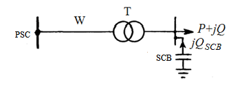
Let the SCB be controlled by the criterion of minimum energy loss. We consider overcompensation invalid, that is, between the reactive power of the load Q (t) and the operating power of the SCB QSCB at any time t, the ratio Q (t) ≥ QSCB must be fulfilled (Fig. 1). As shown in [12], the fulfillment of this condition is also a criterion for optimal control. If the reactive power of the load decreases with time, the next section of the SCB should be switched off only when the full compensation Q(t) = QSCB (cos φ = 1) is reached. Inherent losses of active power in the SCB are small, so the total losses in full compensation mode will be less than losses when one more section of the SCB is disconnected. Thus, any control of the SCB by the criterion of maintaining cos φ at a level less than unity is obviously not optimal.
Fig.1. Electrical network
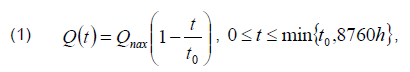
Suppose that the annual reactive power curve can be approximated by a linear function of the following kind [13]:
.
where Qmax is the annual maximum of reactive power; t0 is a graph parameter that characterizes the degree of its filling.
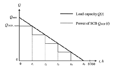
The work [6] show that this approximation gives good results when calculating energy losses. The process of SCB optimal control can be described graphically using the function (1) (Fig. 2).
Fig.2. Example of an annual SCB optimal control diagram
Energy losses in SCB
We introduce the following notation:
QSCB, nom is the rated output of SCB; n is the number of SCB sections; Qс is a single section power; psp is specific losses of active power in SCB (per unit of reactive power generated); Qmin is the annual minimum of the reactive load power.
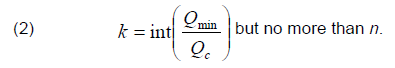
The number of unconnected sections (which are in operation all year round) can be determined by the expression
.
The value of Qmin in the accepted load curve model is determined by the formula (1) when substituting the upper limit of time t. If t0 ≤ 8760 h (which corresponds to the time of using the maximum reactive load Tmax,Q ≤ 4380 h), then the formula (1) gives Qmin = 0. This result may not correspond to real conditions. However, if the actual value of Qmin is not greater than the power of the SCB section, then we do not introduce the error, since the mode of complete shutdown of the SCB does not affect the loss components considered later.
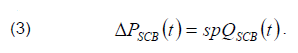
The active power losses of the SCB at every instant is proportional to the reactive power generated:
.
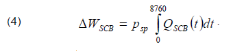
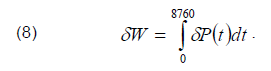
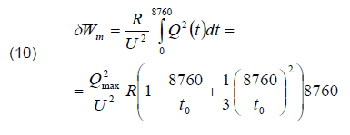
Annual energy losses in SCB are determined by the integral of the form
.
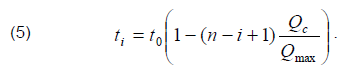
In fact, integration is reduced to summing the products of power losses at each stage of the annual BSC power curve by the duration of the stage (Fig. 2). The borders between ti stages represent the conditional moments of disconnection of the i-th SCB section. From Fig. 2 it directly follows that
.
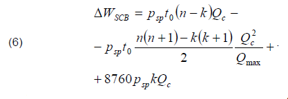
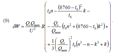
Having performed integration, after some transformations it is possible to obtain the following formula for annual energy losses in SCB:
.
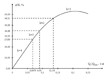
The first two summands together represent energy losses in the disconnected sections, and the last summand means losses in the sections operating without disconnection. Fig. 3 shows an example of the energy losses dependence in the SCB on the power of the section for a four-section SCB at t0= 12000 h (in the area under the load curve this corresponds to Tmax,Q= 5560 h). Energy losses are expressed as a percentage of the losses that would occur under the year-round operation of the SCB with a Qmax capacity (i.e., with full compensation) equal to 8760 psp·Qmax.
The dependence is divided into four segments, which differ from each other in the number of sections k working without disconnection. Full compensation corresponds to the value Qc/Qmax = 0.25. Since it is less than the ratio of the minimum load power to the maximum (0.27 by the formula (1)), the segment where k = 0 is absent in this case.
Segments with different number of k are separated by break points. For k = 4, the dependence is linear. In subsequent segments, there are switching off sections, and the dependence becomes nonlinear resulted from the increase of the section power, when the duration of their operation decreases. At k = 1, the time factor becomes so significant that the dependence passes through the maximum and begins to decrease. The maximum losses in this case are 52.9%, and they are observed at Qc/Qmax = 0.207.
Energy losses in the network
Let us consider the influence of the regulated SCB on power losses in the network from the power supply center (PSC) to the low voltage (LV) buses of the transformer substation (Fig. 1). Formally, this effect applies to both load loss and no-load loss, and it is caused not only by changes in reactive power, but also by changes in voltage at the load node. However, the voltage in the load node depends not only on the capacity of the SCB, but also on the method of voltage regulation in the power center, as well as the modes of the power system as a whole. We assume that there is a counter voltage regulation in the power supply center, at which the voltage in some equivalent load node is maintained at a constant level. Let the LV buses of the substation under consideration correspond approximately to this node. This assumption permits excluding the influence of voltage on energy losses. As a result, we assume that the SCB affects only the load energy losses caused by the transfer of reactive power solely.
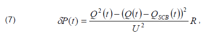
When choosing a SCB, it is not the absolute value of energy losses in the network that matters, but their reduction. Taking into account the accepted assumptions, the losses of active power in the line and transformer (Fig. 1) during the installation of the SCB at each moment reduce by the amount of
.
where R is the total active resistance of the line and transformer; U is the voltage at the load node (usually brought to the high side).
The annual reduction in energy losses in the line and transformer is equal to the integral of power losses reduction:
Fig.3. Dependence of energy losses in a four-section SCB on the section capacity
Fig.4. Dependence of energy losses reduction in the network on capacity of the four-section SCB section
.
After integration and transformations, we finally obtain
.
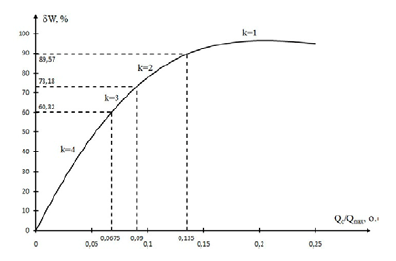
Fig. 4 shows the dependence of reducing energy losses in the network on the power of the SCB section, constructed under the same conditions as in Fig. 3. Reduction of energy losses is expressed as a percentage of losses for reactive power transmission before the SCB installation (in the initial mode), which are equal to
.
The resulting dependence passes through the maximum at Qc/Qmax = 0.207. The maximum loss reduction is 96.8%.
Effect of the number of sections on maximum loss reduction
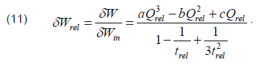
We can write the reduction in energy losses in relative units explicitly by dividing (9) by (10):
.
Let us introduce the following notation:
.
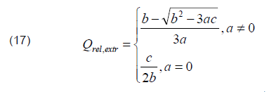
According to formula (11), the dependence of loss reduction on the power of the section in general is a cubic parabola that passes through the maximum at the point of
.
The formula (17) is true if the obtained value falls on the segment of curve δW(Qc), corresponding to the accepted value k. Otherwise, the maximum loss reduction will be located either at another segment of the curve or at the break point (at the segment border).
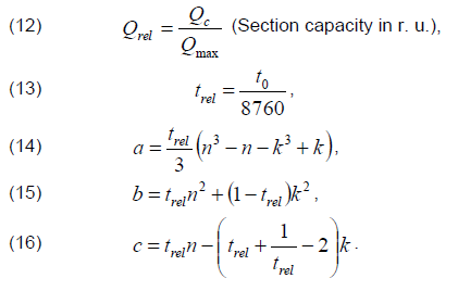
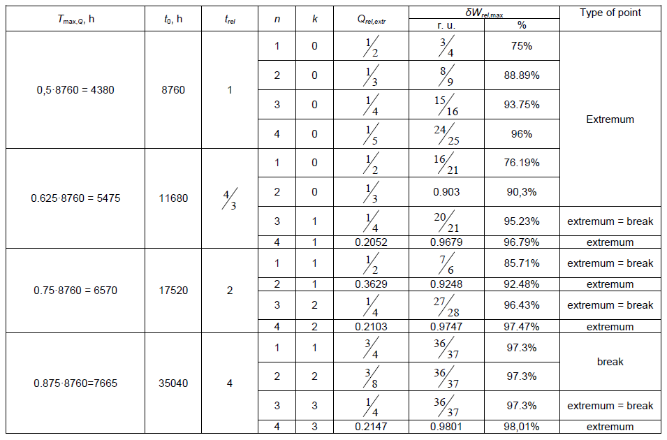
Table 1 shows the results of calculating maximum loss reduction δWrel,max at different times of using the maximum reactive load Tmax,Q and with different quantity of sections. The t0 values were determined on the equality of the areas under the load curves using the formula
.
The calculation was performed in the range of Tmax,Q from 4380 to 0.875·8760=7665 hours. The value of 4380 hours corresponds to the maximum range of changes in the reactive load power. For smaller values of Tmax,Q, the same conditions will be observed as for 4380 hours, but with a reduced time scale. The limit value of Tmax,Q = 8760 hours was not considered, since the load curve becomes uniform, and the SCB will operate without regulation.
Table 1. Results of calculating the maximum loss reduction in the network
.
The maximum reduction in reactive power transmission losses varies from 75% for unregulated SCB and Tmax,Q = 4380 h to 98% for 4-section SCB and Tmax,Q = 7665 h. In the first case, the reactive load changes by 100% during the year, in the second case it changes by 25% of the maximum power. When Tmax,Q = 7665 h the maximum loss reduction practically does not depend on the number of sections, and for the number of sections n = 4, the maximum loss reduction practically does not depend on Tmax,Q, i.e. on the reactive load curve. The most significant effect is observed when switching from an unregulated SCB to a two section SCB.
Conclusions
1. Dependence of energy losses reduction in the network on the SCB capacity, taking into account the regulation, goes through the maximum, with the capacity of the SCB at the maximum point not reaching the highest load power. This means that full power factor compensation is impractical even in cases where the inherent losses in the SCB are small, and its cost can be ignored. This is equally true for unregulated SCB. The exception is a uniform load curve.
2. SCB with two sections allow reducing energy losses for reactive power transmission by 90% or more for almost any load curves. For 3 – and 4-section SCB, the loss reduction is close to 100%. Thus, to reduce energy losses, no more than three or four sections are required, and in most cases, one or two sections are sufficient. A larger number of sections is justified only in cases when it is necessary for voltage regulation.
REFERENCES
[1] Girshin S.S., Bigun A.AY., Petrova E.V., Goryunov V.N., Shepelev A.O., Ivanova E.V. The grid element temperature considering when selecting measures to reduce energy losses on the example of reactive power compensation, Przeglad Elektrotechniczny. 2018, vol. 94, No. 8. 101–104. [2] Zhelezko Yu. S. Power factor compensation in complex electrical systems. – M.: Energoizdat, 1981, 200 p. [3] RTM 36.18.32.6-92 “Instructions for the design of reactive power compensation units in the general-purpose power networks of industrial enterprises”.. [4] Ilyashov V.P. Capacitor installations of industrial enterprises. 3.- Moscow: Energoizdat, 1983, 152 с.. [5] Pasko M., Adrikowski T., Bula D., Blaszczok D. Power losses in the reactive power compensator built of capacitor banks and protective chokes, Przeglad Elektrotechniczny. 2020, vol. 96, No. 3. 166–169. [6] Home-Ortiz J.M., Vargas R., Macedo L.H., Romero R. Joint reconfiguration of feeders and allocation of capacitor banks in radial distribution systems considering voltage-dependent models, International Journal of Electrical Power & Energy Systems. 2019, vol. 107, 298–310. [7] Gonzalo G., Aguila A., Gonzalez D., Ortiz L. Optimum location and sizing of capacitor banks using VOLT VAR compensation in micro-grids, IEEE Latin America Transactions. 2020, vol. 18, 465–472. [8] Abdelhady S., Osama A., Shaban A., Elbayoumi M. Real-Time Optimization of Reactive Power for An Intelligent System Using Genetic Algorithm, IEEE Access. 2020, vol. 8, 11991–12000. [9] Fetouh T., Elsayed A.M. Optimal Control and Operation of Fully Automated Distribution Networks Using Improved Tunicate Swarm Intelligent Algorithm, IEEE Access. 2020, vol. 8, 129689–129708. [10] Muhammad Y., Khan R., Raja M.A.Z., Ullah F., Chaudhary N.I., He Yi. Muha Solution of optimal reactive power dispatch with FACTS devices: A survey, Energy Reports. 2020, vol. 6, 2211–2229. [11] Saddique M.Sh., Bhatti A. R., Haroon Sh.S., Sattar M.K., Amin S., Sajjad I.A., ul Haq S.S., Awan A.B., Rasheedd N. Solution to optimal reactive power dispatch in transmission system using meta-heuristic techniques―Status and technological review , Electric Power Systems Research. 2020, vol. 178, 106031. [12] Girshin S. S., Goryunov V. N., Shepelev A. O. Optimal control of capacitor banks in distribution networks / Scientists of Omsk to the region. Materials of the II Regional scientific and technical conference. Under general ed. L. O. Stripling, Omsk, 2017, 75-79. [13] S. S. Girshin, V. N. Goryunov, A. S. Shiryaev, D. V. Kovalenko. Selection of capacitor banks in electric networks taking into account disconnection at low loads / Industrial power engineering. 2019,no. 12, 12-18.
Authors: Stanilav S. Girshin, Omsk State Technical University, Mira, h. 11, 644050 Omsk, Russian Federation, e-mail: stansg@mail.ru; Aleksandr AY. Bigun, Omsk State Technical University, Mira, h. 11, 644050 Omsk, Russian Federation, e-mail: barsbigun@list.ru; Nikolay А. Mel’nikov, Omsk State Technical University, Mira, h. 11, 644050 Omsk, Russian Federation, e-mail: nik_mel_98@mail.ru; Elena V. Petrova, Omsk State Technical University, Mira, h. 11, 644050 Omsk, Russian Federation, e-mail: evpetrova2000@yandex.ru; Vladislav M. Trotsenko, Omsk State Technical University, Mira, h. 11, 644050 Omsk, Russian Federation, e-mail: troch_93@mail.ru; Dmitry S. Osipov, Yugra State University, Chekhov h. 16, Khanty-Mansiysk, Russian Federation, e-mail: ossipovdmitriy@list.ru; Vladimir N. Goryunov Omsk State Technical University, Mira, h. 11, 644050 Omsk, Russian Federation, e-mail: vladimirgoryunov2016@yandex.ru.
Source & Publisher Item Identifier: PRZEGLĄD ELEKTROTECHNICZNY, ISSN 0033-2097, R. 97 NR 9/2021. doi:10.15199/48.2021.09.23
Published by 1. Mohd Afifi JUSOH, 2. Muhamad Zalani DAUD, 3. Mohd Zamri IBRAHIM, Faculty of Ocean Engineering Technology and Informatics, Universiti Malaysia Terengganu, 21030 Kuala Nerus, Terengganu Malaysia ORCID: 1. 0000-0001-9929-4640; 2. 0000-0003-3003-3068; 3. 0000-0002-9439-8552
Abstract. The inconsistency of solar irradiance and temperature have led to unpredictable output power fluctuation of photovoltaic (PV) system. This paper proposes a simple control scheme for hybrid energy storage (HES) system to mitigate the long-term and short-term output power fluctuations of the PV system. The proposed control scheme employed the fuzzy logic controller in order to manage the power compensation of the HES system and to maintain the state-of-charge (SOC) level of the HES system within safe operating limits during the mitigation process. In the control scheme, the long-term output power fluctuation is eliminated by using battery energy storage, while short-term output fluctuation is compensated using the ultracapacitor. Apart from that, an hourly PV power dispatch was applied in the control scheme since the grid-connected PV system was considered in this study. The simulation evaluations of PV/HES with the proposed control scheme was conducted in the MATLAB/Simulink environment. The effectiveness of the proposed control scheme was verified through several case studies. Initially, the control scheme was evaluated with different initial SOC levels of HES. Then, the control scheme was evaluated using five days of actual PV system output in order to verify the robustness of the proposed control scheme in actual circumstances. Overall, the simulation evaluation was verified that the proposed control scheme of the PV/HES system effectively mitigates the output power fluctuations of the PV system and output power is dispatched out to the utility grid on an hourly basis. Also, it was able to regulate the SOC of HES at the operational limit throughout the process. The simulation result showed the control scheme successfully reduced the unacceptable output power fluctuation from 20% to less than 1%. The results also showed the SOC of HES was regulated within the range of 38%-75% and 42%-60% of its capacity along the process, respectively.
Streszczenie. Niespójność natężenia promieniowania słonecznego i temperatury doprowadziła do nieprzewidywalnych wahań mocy wyjściowej systemu fotowoltaicznego (PV). W niniejszym artykule zaproponowano prosty schemat sterowania hybrydowym systemem magazynowania energii (HES) w celu złagodzenia długo- i krótkoterminowych wahań mocy wyjściowej systemu fotowoltaicznego. Zaproponowany schemat sterowania wykorzystywał sterownik logiki rozmytej w celu zarządzania kompensacją mocy systemu HES i utrzymania poziomu stanu naładowania (SOC) systemu HES w bezpiecznych granicach operacyjnych podczas procesu mitygacji. W schemacie sterowania długoterminowe wahania mocy wyjściowej są eliminowane przez zastosowanie magazynowania energii akumulatora, podczas gdy krótkotrwałe wahania mocy wyjściowej są kompensowane za pomocą ultrakondensatora. Poza tym w schemacie sterowania zastosowano godzinową dyspozytornię mocy fotowoltaicznej, ponieważ w niniejszym opracowaniu uwzględniono system fotowoltaiczny podłączony do sieci. Oceny symulacyjne PV/HES z proponowanym schematem sterowania przeprowadzono w środowisku MATLAB/Simulink. Skuteczność proponowanego schematu kontroli zweryfikowano za pomocą kilku studiów przypadku. Początkowo schemat kontroli oceniano przy różnych początkowych poziomach SOC HES. Następnie schemat sterowania został oceniony przy użyciu pięciu dni rzeczywistej mocy wyjściowej systemu fotowoltaicznego w celu zweryfikowania niezawodności proponowanego schematu sterowania w rzeczywistych warunkach. Ogólnie rzecz biorąc, ocena symulacji została zweryfikowana, że proponowany schemat sterowania systemem PV/HES skutecznie łagodzi wahania mocy wyjściowej systemu fotowoltaicznego, a moc wyjściowa jest wysyłana do sieci energetycznej co godzinę. Ponadto był w stanie regulować SOC HES na limicie operacyjnym podczas całego procesu. Wyniki symulacji wykazały, że schemat sterowania skutecznie zmniejszył niedopuszczalne wahania mocy wyjściowej z 20% do mniej niż 1%. Wyniki pokazały również, że SOC HES był regulowany w zakresie odpowiednio 38%-75% i 42%-60% jego pojemności w trakcie procesu. (Strategia sterowania oparta na logice rozmytej dla godzinowej wysyłki mocy fotowoltaiki podłączonej do sieci z hybrydowym magazynowaniem energii)
Keywords: photovoltaic system, battery energy storage, ultracapacitor, control strategy, fuzzy control Słowa kluczowe: system fotowoltaizny, logika rozmyta, .magazynowanie energii.
1.0 Introduction
Renewable energy (RE) sources have been rapidly developed throughout the world over the past two decades due to fossil fuel depletion and severe environmental pollution. Photovoltaic (PV) energy, is environmental friendly energy that is being considered as a potential replacement for traditional energy sources. However, due to the intermittent nature of solar irradiance and temperature, the output from PV sources are unpredictable, inconsistent and randomly fluctuate [1]. The fluctuation of the output power from PV sources can bring some negative impacts to grid security such as voltage deviation, voltage fluctuation, harmonic and other power quality problems. These problems are some of the obstacles to the efforts of increasing the penetration level of PV power in power grids [2]. In order to reduce these negative impacts, several control strategies have been proposed in the literature for smoothing the output power fluctuations of PV sources, for example in [3]–[11].
One of the methods is mitigation of power fluctuation by geographical dispersion [3]–[5]. Normally, geographical dispersion is used to mitigate the short term output fluctuations for PV clusters installed in a wide area. Another approach is by curtailment of active power by employing Maximum Power Point Tracking (MPPT) controller, which limits the output power of PV sources [6-9]. The conventional method of mitigating the power fluctuation is by using the diesel generator [10], [12]. However, due to slow response and poor efficiency of diesel generator, it leads to difficulty when it comes to handling the high power ramp of PV fluctuations. Furthermore, a diesel generator is not an environmentally friendly solution. Recent trends in power fluctuation mitigation strategy are by using fast response and enhanced flexibility of storage technologies such as battery energy storage (BES), ultracapacitors (UC), flywheel and fuel cells [1], [13]–[15].
Presently, BES and UC are considered great alternatives for mitigating the long-term and short-term output power fluctuations. There are many types of batteries used for BES applications such as flooded leadacid (LA) batteries, valve-regulated lead-acid (VRLA) batteries, nickel-cadmium (NiCd) batteries, lithium-ion (Liion) batteries, sodium-sulfur (NAS) batteries and vanadium redox (VRB) batteries [16]. The various advantages of using an energy storage system in PV system applications are discussed in detail in [16], [17]. The combination of multiple types of energy storage devices with various charge and discharge behaviour is a great solution to mitigate the short-term and long-term output power fluctuations. Thus, this study focuses on the hybridization of Li-ion batteries and UC as a mitigation strategy for output power fluctuations of the PV sources.
From the literature, several control methods have been proposed for mitigating PV output power fluctuations using the HES system that utilizes BES and UC [18]–[21]. In [19], a fuzzy-logic-based adaptive power management system for smoothing PV power output has been proposed. The proposed system managed the power-sharing between UC and BES according to their operational constraints, such as voltage limit, charge/discharge current limit, state-of-charge (SOC) limit, etc. Similarly, a multimode fuzzy logic-based control scheme BES and UC has been proposed in [21]. The control scheme was designed to optimize the operation of BES and UC as well as prevent them from performing under extreme conditions. In this regard, the flexibility of fuzzy logic controllers provide superior performance in many electric power system applications particularly in managing the output power fluctuations of RE sources. The range of fuzzy logic-based applications can also be found in PV system MPPT designs [22] for extracting maximum power from the solar PV system, wind energy generation system or the hybrid wind-PV system. In [19] fuzzy logic has been used in smoothing the solar PV output power fluctuations. Whereas in [10] fuzzy control method has been used for mitigating output power fluctuation by using a diesel hybrid power system. The proposed method is necessary for considering the conflicting objective of maximizing energy captive and output power levelling. The simulation results showed that the proposed method was feasible in levelling output power fluctuations and reducing the frequency deviation. In [23], an optimal hourly energy management system for hybrid wind, PV system, hydrogen and battery system with supervisory control based on fuzzy logic has been developed. The fuzzy logic controller is used in an hourly energy management system to maintain the energy flow while optimizing the utilization cost and lifetime of the energy storage system.
This paper proposes a fuzzy logic-based hourly dispatch control scheme for a grid-connected PV system with HES (PV/HES) system. The objective is to design the optimal control scheme for a hybrid PV system with BES and UC to reduce the output power fluctuation from the PV system. The presented control scheme offers superior reliability and effective performance for the PV/HES system. The simulation results demonstrated that the control scheme could maintain the system operation of PV/HES within the desired limitations while dispatching a stable output power to the grid system. The main contribution of this paper can be described based on the control scheme that has been developed for regulating the charging and discharging of BES and UC to smooth out the PV output power fluctuations.
The rest of the paper is organized as follows: Section 2 generally describes the grid-connected PV/HES system considered in the present study. Section 3 describes the modelling process of grid-connected PV/HES system for simulation studies. Section 4 presents the proposed fuzzylogic based control scheme. Section 5 provides the simulation results and discussion and Section 6 concludes the paper.
2.0 Grid-Connected PV/HES system
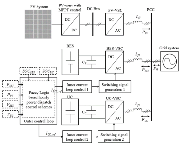
The overall system configuration of the hybrid PV/HES system with the proposed control scheme is shown in Fig. 1. Based on the figure, the grid-connected and ac-coupled concept of PV/HES was considered in the present study. The figure shows grid-connected PV system is parallelly connected to HES at the point of common coupling (PCC) bus via a voltage-sourced converter (VSC).
The purpose of the BES-VSC and UC-VSC is to regulate the fluctuated output power from the PV system (PPV) according to the reference signal from the fuzzy-based controller. The power is injected into the grid system through the charging/discharging of BES power (PBES) and UC power (PUC). In this regard, the net power (PG) is delivered to the utility system according to the hourly setpoint (PSET) as illustrated in Fig. 1. PSET is considered as the forecasted output power set point that has been obtained from average PPV output using the forecasting model from [24].
Fig.1. Grid-connected PV/HES system configuration for hourly output power dispatch strategy
3.0 Modelling and simulation of hybrid PV with BES and UC system
This section describes how the PV power output, PPV is obtained. Then, the estimation of the hourly set-point, PSET data to be used by the fuzzy control scheme is presented. The grid-connected PV system considered in the present study is based on the performance of large scale PV system in Malaysia.
3.1 Modelling of PV power output (PPV) and Hourly setpoint (PSET)
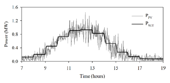
To evaluate the proposed control scheme for PV/HES system, the PV system output data and output power setpoint data for hourly power dispatch of PV source are necessary. Fig. 2 shows the average daily PPV profile for a 1.2 MW PV system which has been analyzed from the Malaysian historical radiation and temperature data in [24]. The average hourly solar radiation was preliminarily analyzed in Matlab by using statistics to represent the average one-day input data of a PV system. The data was then altered by adding random noise data in order to represent the real output of the considered PV system. The added random noise data were extracted based on the nominal Malaysian weather characteristic, in which the major intermittent clouds occurred during the middle of the day between 11 AM to 3 PM. To provide accurate PPV profile data, 5% losses of the power converter is also considered with MPPT operation taken into account.
Besides that, Fig. 2 also presents the PSET curve that was calculated from the hourly average of the PPV profile with 10% added mean absolute error (MAE) noise data to represent the forecast accuracy of the PV output forecasting model. The rate limiter is also applied to PSET to minimize the output power ramps of the PV system and prevents overshooting when PSET changes.
Fig.2. Simulated typical average daytime (7 AM to 7 PM) operation of a PV farm at Subang Jaya, Kuala Lumpur [25]
3.2 Modelling of BES system
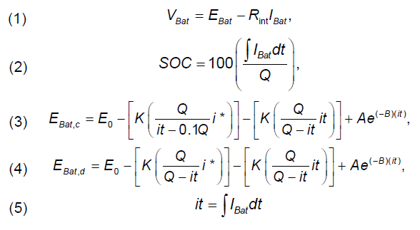
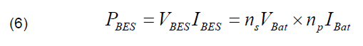
The Li-ion battery was considered as BES because of its excellent features, such as high efficiency and high energy density. The battery model was developed based on a dynamic battery model, as described in [26]. The battery model is represented by the equations to describe the electrochemical behaviour of a battery in terms of the state of charge, terminal voltage, cell temperature and internal resistance. The formulated equations of the BES are described using Eq. 1 to Eq. 5, where VBatis the battery voltage (V), EBat,c and EBat,d are the battery electromotive force during charge and discharge (V). IBat is the battery current (A) and Rint is the battery internal resistance (Ω). Q is the cell battery capacity (Ah) and EO is battery open-circuit voltage (V). K is Polarisation resistance (Ω), i* is filtered current (A) and it is actual battery current (Ah). A is exponential zone voltage (V) and B is exponential zone time constant inverse (Ah-1)
.
By combinations of the series and parallel battery cell, BES model can be constructed as follow:
.
where ns is the number of cell in series and np is the number of cell in parallel, respectively. The number of cells in series and parallel determines total output terminal voltage and capacity or total size of a battery bank respectively. All of the parameters for the battery model can be approximated by using the manufacturer’s data following the procedures in [26]. For the battery model, there are several specific assumptions and limitations such as there is no self-discharge, the nominal capacity and internal resistance constant and there are no environmental considerations.
3.3 Modelling of UC
The electric double-layer capacitor (EDLC) is selected as a short term energy storage due to its advantages such as fast charge/discharge process, high power density, and extended lifetime. For the simulation studies, the EDLC model is developed based on the dynamic equivalent circuit, described in [2].
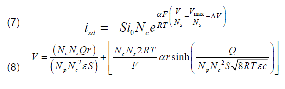
The mathematical model of dynamic EDLC consists of Stern and Tafel equations which relate to voltage, current and the available charge of the EDLC. The Tafel equation is used to calculate the self-discharge of EDLC and the Stern equation is used to calculate the voltage of the controlled voltage source. The Tafel and Stern equation is described as follows [17]:
.
where Nsand Np are the numbers of series and parallel EDLC cells. Nc is the number of electrodes layers, Q is the electric charge (C), r is the molecular radius (m) and ε permittivity of the material. S is the interfacial area between electrodes and electrolyte (m2), R is the ideal gas constant, T is operating temperature (F), α is charge transfer coefficient, c is the molar concentration (molm-3), i0 is exchanged current density, F is Faraday constant, Vmax is surge voltage (V) and ΔV is over-potential voltage (V). The details of parameters and calculation are described in [27].
4.0 Fuzzy-Based Hourly Dispatch Control Strategy
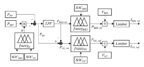
A fuzzy logic controller is well-known as an effective technique to control various kinds of complex systems [28]. In the present study, a fuzzy controller is considered to control the operation of PV/HES in order to provide stable output power to the grid system. Fig. 3 shows the proposed fuzzy-based control scheme with hourly dispatch for a hybrid PV/HES system.
Fig.3. The diagram of a proposed fuzzy-based control scheme for PV/BES
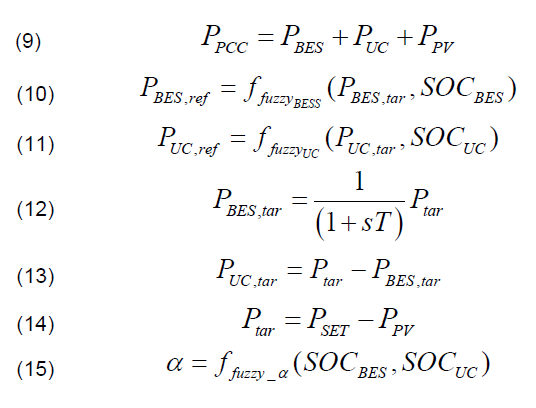
As shown in the figure, the fuzzy logic-based control scheme consists of two major layers. The first layer is the adjustment of power set-point level, PSET, in which fuzzyα adjusts the PSET of the PV output depending on the overall SOC level of BES and UC (SOCBES & SOCUC), respectively. The second layer is the adjustment of energy storage power dispatch, where fuzzyBES and fuzzyUCadjust the power dispatching of BES and UC depending on their SOC levels, respectively. As illustrated in Fig. 3, PPV and PSET are inputs of the control scheme and the deviation between PPV and PSET is a target power (Ptar) for the BES and UC to charge and discharge the power. Ptar is filtered using first order low pass filter (LPF) to ensure that the UC storage device compensates for sudden changes in the rapidly fluctuating PV output power while the BES storage device covers the long-term fluctuating PV output. The filtered outputs from LPF (PBES,tar& PUC,tar), SOCBES and SOCUC are used as inputs of fuzzyBESand fuzzyUC to regulate the reference for BES and UC (PBES,ref & PUC,ref) in order to dispatch the power to the PCC, respectively. So that the PV system output power is smoothed out. The control scheme in Fig. 3 can be formulated based on Equation (9)-(15).
.
4.1 Fuzzy logic-based hourly set-point control fuzzy_α
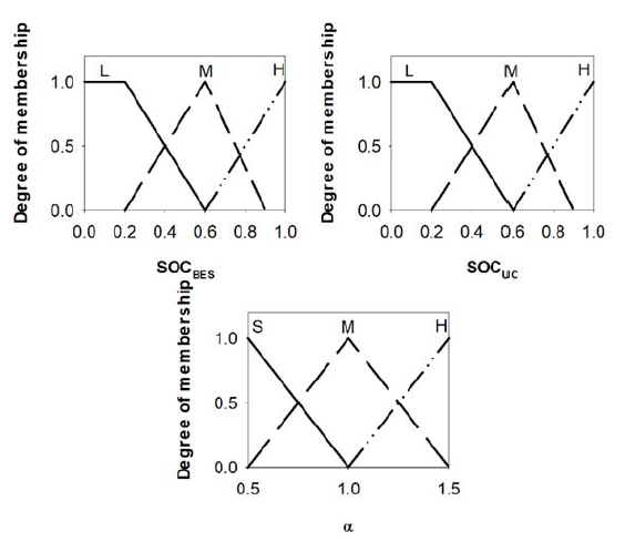
Fuzzy logic control for PSETadjustment, fuzzyα is designed to alter the PSET level based on SOCBES and SOCUC, respectively by applying the coefficient (α) to the PSET level. The coefficient greatly determines the charging and discharging levels of BES and UC, respectively. During the low level of SOCBES and SOCUC, the fuzzyα adjusts the α to decrease the PSET level which means that more power and energy needs to be charged by the BES and UC, respectively. Whereas during the high level of SOCBES and SOCUC, the fuzzyα regulates the α to increase the PSET level which means that more energy is required to be compensated by the BES and UC, respectively. Fig. 4 shows the membership function of fuzzyα. The input membership function contains three levels; low (L), medium (M) and high (H), while the output membership function contains three levels; small (S), medium (M) and high (H). The fuzzy rules are described as follows:
1. If SOCBES is L or SOCUC is L then output is S 2. If SOCBES is M or SOCUCis M then output is M 3. If SOCBES is H or SOCUC is H then output is H
Fig.4. Membership function of fuzzyα
4.2 Fuzzy logic-based BES power control (fuzzyBES)
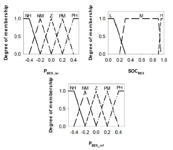
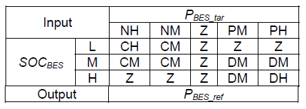
Fuzzy logic controller for BES, fuzzyBES consists of two inputs and one output as shown in Fig. 3. The fuzzyBES is designed to adjust the PBES,tar according to the SOCBES level. The input and output membership functions of the fuzzyBES are as shown in Fig. 5, respectively. Five levels of PBES,tar membership function are considered; NH, NM, Z, PM and PH where N stands for Negative, Z for zero, P for positive, M for medium and H for high to perform a compromise between the accuracy of the power control and its complexity. While three levels of SOCBES membership functions are considered; low (L), medium (M) and high (H) to accommodate the needs of the proposed strategy. The low level and high level of SOCBES represent the energy reserve to avoid the over-charging and over-discharging of BES while the medium level is used to compensate for the long-term PV power fluctuation around the PBES,tar. PBES,ref represents the output of fuzzyBES membership function. Five levels are considered for positive and negative power reference; CH, CM, Z, DM and DH where C stands for a charge, Z for zero, D for discharge, M for medium and H for high. The fuzzy rules of fuzzyBES are designed to prevent the BES from energy depletion. The rules are described in Table 1.
Fig.5. Membership function of fuzzyBES
Table 1. Fuzzy rules of fuzzyBES
.
4.3 Fuzzy logic-based UC power control (fuzzyUC)
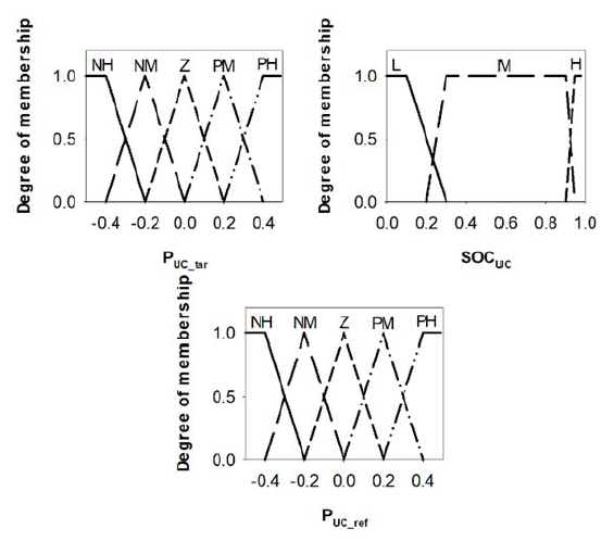
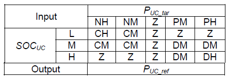
Fuzzy logic controller for UC, fuzzyUC consists of two inputs and one output as shown in Fig. 3. PUC,tar and SOCUC are chosen as input of the fuzzyUC. The fuzzyUC regulates PUC,tar according to SOCUC level to ensure the sustainability of UC energy. The output from the controller is PUC,ref that will be used by the UC to charge/discharge its power. The input and output membership function of the controllers are as shown in Fig. 6, respectively.
Five levels of PUC,tar membership function are considered; NH, NM, Z, PM and PH where N stands for Negative, Z for zero, P for positive, M for medium and H for high, while three levels of SOCUC membership function are considered; low (L), medium (M) and high (H) as illustrated in Fig. 6. The low level and high level of SOCUC represent the energy saturation to keep the UC in the safe operation during charging and discharging. The medium level of UC is used to compensate for the short-term PV power fluctuation. For the PUC,ref, five levels are considered; CH, CM, Z, DM and DH where C stands for the charge, Z for zero, D for discharge, M for medium and H for high. The fuzzy rules of fuzzyUC are described in Table 2.
Fig.6. Membership function of fuzzyUC
Table 2. Fuzzy rules of fuzzyUC
.
5.0 Results and discussion
In this paper, the effectiveness of the proposed control scheme in order to provide an adequate smoothing of PV output power fluctuations is examined through the simulation. The performance evaluation of the proposed control scheme based on the cases the study results are discussed in Section 5.1 and then the evaluation results of the proposed control scheme using actual five-day PV output power data is discussed in Section 5.2.
5.1 Result of analysis based on the difference of initial SOC of BES and UC
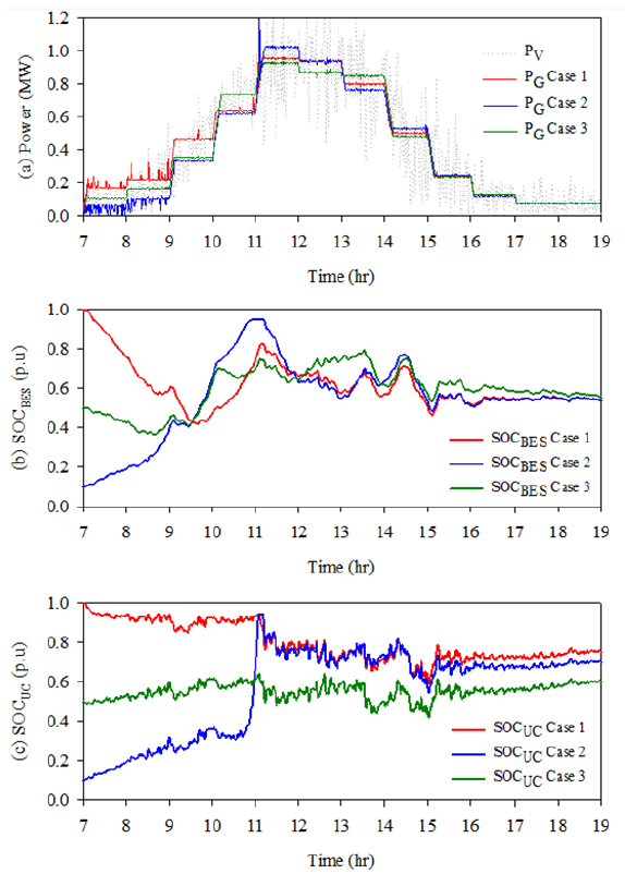
The proposed fuzzy-based control scheme was initially evaluated by three case studies of the initial SOC level of HES. In these cases, the initial SOCBES and SOCUC were set to 100%, 50% and 10%, respectively. Fig. 7 provides the result of PSET adjustment for different case studies, while Fig. 8 shows the simulation result of the output power, SOCBES and SOCUC profiles, for three different cases studied, respectively. The following describes the conditions of each case study.
5.1.1 Case 1: SOC set at 100%
For case 1, the initial SOCBES and SOCUC were set to 90% which is the highest SOC level for the BES and UC. In this case, during the high SOC level of BES and UC, the proposed controller efficiently adjusts the hourly set point, PSET level as illustrated in Fig. 7. As indicated in Fig. 7, the PSET was increased to switch the BES and UC device to discharge mode. So, the BES and UC can discharge more power to the PCC in order to maintain their SOC level at the nominal SOC state, as shown in Fig. 8(a). From Figure 8(b) and (c), the SOCBES and SOCUC can be efficiently restored to their nominal capacity state after several hours of operation without the need for additional energy storage capacity. Also, the maximum PPV can be transferred to the grid system.
5.1.2 Case 2: SOC set at 10%
For case 2, the initial SOCBES and SOCUC were set to 10% and which is the lowest SOC level for the BES and UC, respectively. In this case, during the low SOC level of BES and UC, the proposed control scheme adjusts to reduce the PSET level, as shown in Fig. 7. So that, the BES and UC can be changed to charge mode in order to restore their energy at the nominal SOC state. As indicated in Fig. 8(a)-(c), more PPV is used to charge and discharge HES instead of the PPV injected into the grid system. From the simulation results, it was verified that the proposed control scheme efficiently managed the BES and UC to restore their energy at the nominal SOC state.
5.1.3 Case 3: SOC set at 50%
For case 3, the initial SOCBES and SOCUC were set to 50%, which was considered as a nominal SOC level of BES and UC. In this case, the PSET level remains unchanged throughout the process, as demonstrated in Fig. 7. This is due to the energy balance of the BES and UC which enables BES and UC to charge and discharge the energy during the mitigation process, as shown in Fig. 8(b) and (c). The figures also show the SOCBES and SOCUC remain stable until the end of the simulation.
Fig.7. PSET adjustment for different cases
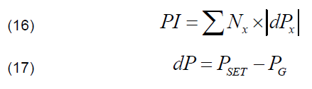
In addition, the comparison of the PV/HES performance with and without the proposed control scheme also is discussed in the present study. In this case, the performance index, PI of the PV/BES system was firstly determined using the following equations [29]:
.
where, dP is the deviation of the total power transfer to the grid, PGand the PSET . PG is the power measured at the PCC bus. Nx is the number of dP. In this case, the acceptable dP is set to ±10% of the PV system capacity, as suggested in [30].
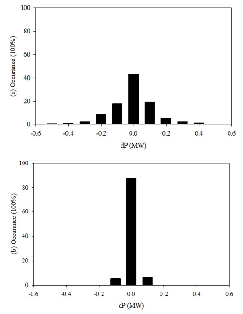
The result of PI is illustrated in Fig. 9. From Fig. 9(a), it can be observed that without the proposed control scheme, a large unacceptable power fluctuation has occurred. The result shows that without the proposed control scheme, the total of unacceptable dP is found to be approximately 20% of the total occurrences. Also, only 50% of PG meets the PSET level during the dispatching process. However, for the case using the proposed control scheme, the unacceptable deviations greatly decreased to less than 1%, as shown in Fig. 9(b). The result also shows 90% of the PG meets the PSET level during the dispatching process.
Fig.8. Simulation results of three different cases. (a) PPV and PG profiles, (b) SOCBES profile and (c) SOCUCprofile
Fig.9. Comparison of PI. (a) Without proposed control scheme and (b) With a proposed control scheme
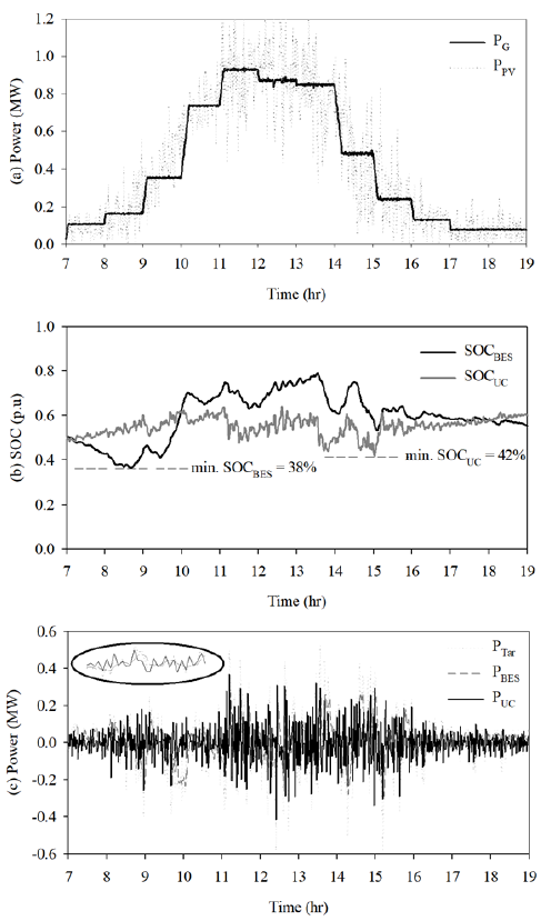
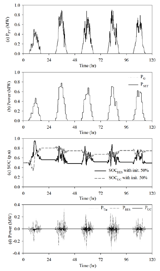
Fig. 10 demonstrates the simulation results of the system performance during the nominal condition, in which the initial SOCBES and SOCUC were set to 50%. The dispatching performance of the PV/HES system is shown in Fig. 12(a) whereas the corresponding SOC profile and power profile of BES and UC are shown in Fig. 10(b) and (c), respectively. As indicated in Fig. 10(a) and (b), PSET can be tracked perfectly while keeping the SOCBES and SOCUC level at the desired operational constraints. From Fig. 10(a), the power fluctuation of the PV system is successfully smoothed out and dispatched out to the utility grid on an hourly basis. Consequently, Fig. 10(b) shows that SOCBES and SOCUC are regulated and varied within the acceptable operational range, which is within 38%-75% and 42%-60%, respectively throughout the process. The power compensated by BES and UC during the smoothing process are illustrated in Fig. 10(c) and it is observed that BES and UC are used to mitigate long-term and short term output fluctuationns, respectively.
Fig.10. Simulation result using 50% of initial SOC. (a) PPV and PG profiles, (b) SOCBES and SOCUC profiles, and (c) Ptar, PBES and PUC profiles
5.2 Simulation results of the proposed controller applied to actual PV output data
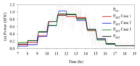
The proposed control scheme is further validated using actual PV system output data. The purpose of the simulation is to evaluate the robustness of the proposed control scheme in actual circumstances. In this case, typical five minute resolution data for five days are collected from a 3 kWp rooftop PV system [30]. The data magnitude was scaled 4 times to represent a 1.2 MW size of PV system for the comparison purpose, as shown in Fig. 11(a). From the figure, it can be seen the impact of intermittent clouds on PV system output causes power fluctuation injected into the utility grid. Overall, the fluctuated PPV normally occurs between 11 AM to 3 PM. During such a situation, it may cause problems and instability of grid operation such as frequency deviation, voltage rise and dip, voltage deviations, prolonged power fluctuation, etc. These power fluctuation problems can be mitigated using the proposed control scheme, as shown in Fig. 11(b). From the figure, it can be seen the fluctuated PPV are successfully smoothed out and dispatched to the utility grid on an hourly basis. During the power dispatching process, the SOCBES and SOCUC operational constraints are kept at the acceptable operational limits, as illustrated in Fig. 11(c). The power compensated by BES and UC throughout the process is shown in Fig. 11(d).
Fig.11. Evaluation of proposed control scheme using five days actual data. (a) PPV profile, (b) PG and PSET profiles, (c) SOCBES and SOCUC profiles, and (d) Ptar, PBES and PUC profiles
6.0 Conclusion
This paper proposed a fuzzy logic-based control scheme for hourly dispatch of fluctuated PV system output using the HES system. The HES comprises UC and BES energy storage devices which are used to mitigate the long-term and short-term output fluctuation of the PV system. The control scheme was developed to ensure the safe operation of the storage system while continuously providing energy support for power fluctuation mitigation. Initially, the simulation results based on several initial SOC conditions have demonstrated the effectiveness of the proposed control scheme. The results show using the proposed control scheme the unacceptable power fluctuations of the PV system was successfully reduced from 20% to less than 1%. The results also show the proposed control scheme efficiently managed the SOCBES and SOCUC within its operational limit throughout the process. It can be seen that during the nominal initial SOC case, the SOCBES and SOCUC were measured between 38%-75% and 42%-60%, respectively. Finally, the robustness of the proposed system was evaluated using five days of actual PV system output data. The evaluation result shows that a proposed control scheme is able to manage the output fluctuation of a PV system over 5 days of operation without any failure of energy support from the HES. In conclusion, since a simple fuzzy controller was used in the proposed control scheme, it can be easy to implement in real-time applications, particularly for renewable energy-based power fluctuation mitigation strategies. Also, it is suggested that further experimental validation of the proposed control scheme is needed to verify its performance in the real application.
Acknowledgements The authors would like to acknowledge Universiti Malaysia Terengganu for the financial support of this research. This research is supported by Universiti Malaysia Terengganu under the UMT TAPE-RG grant, vot. no. 55221.
REFERENCES
[1] S. Shivashankar, S. Mekhilef, H. Mokhlis, and M. Karimi, “Mitigating methods of power fluctuation of photovoltaic (PV) sources – A review,” Renew. Sustain. Energy Rev., vol. 59, pp. 1170–1184, Jun. 2016, doi: 10.1016/j.rser.2016.01.059. [2] T. T. Trung, S. J. Ahn, J. H. Choi, S. Il Go, and S. R. Nam, “Real-time wavelet-based coordinated control of hybrid energy storage systems for denoising and flattening wind power output,” Energies, vol. 7, no. 10, pp. 6620–6644, Oct. 2014, doi: 10.3390/en7106620. [3] J. Marcos, L. Marroyo, E. Lorenzo, and M. García, “Smoothing of PV power fluctuations by geographical dispersion,” Prog. Photovoltaics Res. Appl., vol. 20, no. 2, pp. 226–237, Mar. 2012, doi: 10.1002/pip.1127. [4] M. Lave, J. Kleissl, and E. Arias-Castro, “High-frequency irradiance fluctuations and geographic smoothing,” Solar Energy, vol. 86, no. 8. Pergamon, pp. 2190–2199, Aug. 01, 2012, doi: 10.1016/j.solener.2011.06.031. [5] T. E. Hoff and R. Perez, “Quantifying PV power Output Variability,” Sol. Energy, vol. 84, no. 10, pp. 1782–1793, Oct. 2010, doi: 10.1016/j.solener.2010.07.003. [6] M. Z. Daud, A. Mohamed, and M. A. Hannan, “A novel coordinated control strategy considering power smoothing for a hybrid photovoltaic/battery energy storage system,” J. Cent. South Univ., vol. 23, no. 2, pp. 394–404, Feb. 2016, doi: 10.1007/s11771-016-3084-2. [7] P. P. Zarina, S. Mishra, and P. C. Sekhar, “Exploring frequency control capability of a PV system in a hybrid PV-rotating machine-without storage system,” Int. J. Electr. Power Energy Syst., vol. 60, pp. 258–267, Sep. 2014, doi: 10.1016/j.ijepes.2014.02.033. [8] R. Tonkoski, L. A. C. Lopes, and T. H. M. El-Fouly, “Coordinated active power curtailment of grid connected PV inverters for overvoltage prevention,” IEEE Trans. Sustain. Energy, vol. 2, no. 2, pp. 139–147, Apr. 2011, doi: 10.1109/TSTE.2010.2098483. [9] M. A. Jusoh and M. Z. Daud, “Particle swarm optimisationbased optimal photovoltaic system of hourly output power dispatch using Lithium-ion batteries,” J. Mech. Eng. Sci., vol. 11, no. 3, pp. 2780–2793, Sep. 2017, doi: 10.15282/jmes.11.3.2017.1.0252. [10] M. Datta, T. Senjyu, A. Yona, T. Funabashi, and C. H. Kim, “A frequency-control approach by photovoltaic generator in a PVdiesel hybrid power system,” IEEE Trans. Energy Convers., vol. 26, no. 2, pp. 559–571, Jun. 2011, doi: 10.1109/TEC.2010.2089688. [11] M. A. Jusoh and M. Z. Daud, “Control strategy of a gridconnected photovoltaic with battery energy storage system for hourly power dispatch,” Int. J. Power Electron. Drive Syst., vol. 8, no. 4, pp. 1830–1840, Dec. 2017, doi: 10.11591/ijpeds.v8i4.pp1830-1840. [12] J. S. Park, T. Katagi, S. Yamamoto, and T. Hashimoto, “Operation control of photovoltaic/diesel hybrid generating system considering fluctuation of solar radiation,” Sol. Energy Mater. Sol. Cells, vol. 67, no. 1–4, pp. 535–542, Mar. 2001, doi: 10.1016/S0927-0248(00)00325-1. [13] M. Z. Daud, A. Mohamed, M. A. Hannan, “A review of the intergration of Energy Stroage Systems (ESS) for utility grid support,” PRZEGLAD ELEKTROTECHNICZNY, vol. Jan. 2011, vol. 10a/2012, pp. 185–191 [14] B. Boumediene, A. Smaili, T. Allaoui, A. Berkani and F. Marignett, “Backstepping control strategy for multi-source energy system based flying capacitor inverter and PMSG,” in PRZEGLAD ELEKTROTECHNICZNY, vol. 3/2021, pp. 21Proceedings, 2007, pp. 21-29, doi:10.15199/48.2021.03.04. [15] C Sourkounis, B Ni, F Richter, ” Comparison of energy storage management methods to smooth power fluctuations of wind parks”, PRZEGLAD ELEKTROTECHNICZNY, vol. 10/2009, pp.196-200, doi: [16] X. Tan, Q. Li, and H. Wang, “Advances and trends of energy storage technology in Microgrid,” Int. J. Electr. Power Energy Syst., vol. 44, no. 1, pp. 179–191, Jan. 2013, doi: 10.1016/j.ijepes.2012.07.015. [17] M. Sechilariu, B. Wang, and F. Locment, “Building integrated photovoltaic system with energy storage and smart grid communication,” IEEE Trans. Ind. Electron., vol. 60, no. 4, pp. 1607–1618, 2013, doi: 10.1109/TIE.2012.2222852. [18] N. S. Jayalakshmi, D. N. Gaonkar, J. V. Kumar, and R. P. Karthik, “Battery-ultracapacitor storage devices to mitigate power fluctuations for grid connected PV system,” Mar. 2016, doi: 10.1109/INDICON.2015.7443500. [19] Y. Ye, R. Sharma, and D. Shi, “Adaptive control of hybrid Ultracapacitor-Battery storage system for PV output smoothing,” in American Society of Mechanical Engineers, Power Division (Publication) POWER, Feb. 2013, vol. 2, doi: 10.1115/POWER2013-98210. [20] M. E. Glavin and W. G. Hurley, “Optimisation of a photovoltaic battery ultracapacitor hybrid energy storage system,” Sol. Energy, vol. 86, no. 10, pp. 3009–3020, Oct. 2012, doi: 10.1016/j.solener.2012.07.005. [21] X. Feng, H. B. Gooi, and S. X. Chen, “Hybrid energy storage with multimode fuzzy power Allocator for PV systems,” IEEE Trans. Sustain. Energy, vol. 5, no. 2, pp. 389–397, Apr. 2014, doi: 10.1109/TSTE.2013.2290543. [22] T. H. Kwan and X. Wu, “Maximum power point tracking using a variable antecedent fuzzy logic controller,” Sol. Energy, vol. 137, pp. 189–200, Nov. 2016, doi: 10.1016/j.solener.2016.08.008. [23] P. García, J. P. Torreglosa, L. M. Fernández, and F. Jurado, “Optimal energy management system for stand-alone wind turbine/photovoltaic/ hydrogen/battery hybrid system with supervisory control based on fuzzy logic,” Int. J. Hydrogen Energy, vol. 38, no. 33, pp. 14146–14158, Nov. 2013, doi: 10.1016/j.ijhydene.2013.08.106. [24] J. Cao and X. Lin, “Study of hourly and daily solar irradiation forecast using diagonal recurrent wavelet neural networks,” Energy Convers. Manag., vol. 49, no. 6, pp. 1396–1406, Jun. 2008, doi: 10.1016/j.enconman.2007.12.030. [25] M. Z. Daud, A. Mohamed, A. A. Ibrahim, and M. A. Hannan, “Heuristic optimization of state-of-charge feedback controller parameters for output power dispatch of hybrid photovoltaic/battery energy storage system,” Meas. J. Int. Meas. Confed., vol. 49, no. 1, pp. 15–25, Mar. 2014, doi: 10.1016/j.measurement.2013.11.032. [26] O. Tremblay and L. A. Dessaint, “Experimental validation of a battery dynamic model for EV applications,” World Electr. Veh. J., vol. 3, no. 2, pp. 289–298, Jun. 2009, doi: 10.3390/wevj3020289. [27] “Implement generic supercapacitor model – Simulink.” https://www.mathworks.com/help/physmod/sps/powersys/ref/supercapacitor.html (accessed May 19, 2021). [28] L. Suganthi, S. Iniyan, and A. A. Samuel, “Applications of fuzzy logic in renewable energy systems – A review,” Renew. Sustain. Energy Rev., vol. 48, pp. 585–607, 2015, doi: 10.1016/j.rser.2015.04.037. [29] S. Teleke, M. E. Baran, A. Q. Huang, S. Bhattacharya, and L. Anderson, “Control strategies for battery energy storage for wind farm dispatching,” IEEE Trans. Energy Convers., vol. 24, no. 3, pp. 725–732, 2009, doi: 10.1109/TEC.2009.2016000. [30] M. Z. Daud, A. Mohamed, and M. A. Hannan, “An improved control method of battery energy storage system for hourly dispatch of photovoltaic power sources,” Energy Convers. Manag., vol. 73, pp. 256–270, Sep. 2013, doi: 10.1016/j.enconman.2013.04.013.
Authors: Mohd Afifi Jusoh, Renewable Energy and Power Research Interest Group (REPRIG), Eastern Corridor Renewable Energy SIG, Faculty of Ocean Engineering Technology and Informatics, Universiti Malaysia Terengganu, 21030 Kuala Nerus, Terengganu Malaysia. Email: mohd.afifi.jusoh@gmail.com; Assoc. Prof. Ts. Dr. Muhamad Zalani Daud (Corresponding Author), Renewable Energy and Power Research Interest Group (REPRIG), Eastern Corridor Renewable Energy SIG, Faculty of Ocean Engineering Technology and Informatics, Universiti Malaysia Terengganu, 21030 Kuala Nerus, Terengganu Malaysia. Email: zalani@umt.edu.my Prof. Ts. Dr. Mohd Zamri Ibrahim, Renewable Energy and Power Research Interest Group (REPRIG), Eastern Corridor Renewable Energy SIG, Faculty of Ocean Engineering Technology and Informatics, Universiti Malaysia Terengganu, 21030 Kuala Nerus, Terengganu Malaysia. Email: zam@umt.edu.my
Source & Publisher Item Identifier: PRZEGLĄD ELEKTROTECHNICZNY, ISSN 0033-2097, R. 98 NR 1/2022. doi:10.15199/48.2022.01.02
Published by Kris Scicluna 1,* , Brian Azzopardi 1,2 and Kurt Spiteri 1, (1) Institute of Engineering & Transport, Malta College of Arts, Science and Technology, PLA 9032 Paola, Malta; brian.azzopardi@mcast.edu.mt (B.A.) (2) The Foundation for Innovation and Research—Malta, BKR 4012 Birkirkara, Malta *Correspondence: kris.scicluna@mcast.edu.mt; Tel.: +356-7986-8731
Abstract: This paper presents a power quality analysis for multiple electric vehicle charging stations of the AC-Level 2 type in a real-life case study. The data was collected with a power quality analyzer that measured the main distribution system feeding nine 7 kW charging stations in a commercial site with light-duty vehicles in Malta, Europe. The relevance of this study to the specific case of Malta is accentuated by the topological challenges of the country; high density of road vehicles, with 18,000 vehicles for each square kilometer; and ambitious targets of reaching carbon neutrality by 2050. Data were collected over six days on an actual charging system with real-life charging patterns. Various results are presented in this paper, including three-phase system voltages and currents, individual harmonic voltage and current components, total harmonic distortion and total current demand distortion. These measurements were compared with standardized thresholds for low-voltage equipment used in public spaces, mainly as stated in IEEE 519-2014.
Keywords: electric vehicle; charging; power quality; harmonic analysis; Type 2 chargers; total harmonic distortion
1. Introduction
This paper presents a power quality (PQ) analysis for an electrical system with nine electrical vehicle charging stations of the AC-Level 2 type (unidirectional) in a real-life case study connected to a 400 V low voltage (LV) electrical grid. The data was collected with an experimental setup that consisted of a power quality analyzer sampling measurements on the main distribution system feeding the nine 7 kW charging stations in a commercial site with a fleet of light-duty service vehicles in Malta, Europe. The territory of Malta is relatively small, covering a total area of around 316 square kilometres (122 square miles). Despite its relatively small size, Malta is densely populated, with a population of over 500,000 people. The main island of Malta itself accounts for the majority of the land area, while the smaller islands of Gozo and Comino make up the rest of the national territory. The territory provides a possibly unique case to evaluate the effects of modern power electronics equipment on PQ.
The Malta Low Carbon Development Strategy [1] outlines the country’s goals for the reduction in greenhouse gas emissions through strategies in various sectors, including transportation, buildings, industry, waste management, water management and agriculture. The greenhouse gas (GHG) emissions per capita and GHG emissions per unit of gross domestic product (GDP) have been reduced significantly in Malta since 2014. Malta also stands below the European Union (EU) average in terms of GHG emissions per capita. However, further efforts in reducing GHG emissions are necessary to meet the following:
• 2030 targets under Regulation (EU) 2018/842 of the European Parliament and the Council binding annual GHG emissions reductions from 2021 to 2030 by Member States contributing to climate action to meet commitments under the Paris Agreement and amending Regulation (EU) No. 525/2013.
• Malta’s decarbonization plans, which are in line with those adopted by the EU of reaching climate neutrality by 2050.
A significant part of the strategy in the transportation sector identified in [1] is reliant on the electrification of vehicles and sourcing power for such vehicles through renewable methods. Malta has a high density of vehicles, with 18,000 vehicles for each square kilometre, translating to 1500 cars for every 1000 drivers. Hence, efforts in this area are expected to be highly impactful towards decarbonization goals.
The impact of renewable energy, which today is mostly driven by switching electronic power converters, in the particular case of Malta has already been investigated in [2–5] and the particular effects of electric vehicles on the grid were modelled in [6]. The island provides an interesting case scenario for the uptake of light-duty electric vehicles (EVs) since the electrical grid is predominantly a centralized one with the only distributed sources of generation being of the renewable type. Given the natural topological challenges to upgrading the electrical infrastructure, Malta relies on distribution systems and routes that were not originally designed for distributed generation and storage. Hence, the evaluation of EV charging infrastructure as presented in this paper is possibly of a more critical nature than in other countries with more extensive national boundaries and fewer infrastructural challenges.
Electric vehicle chargers are subdivided into three categories [7,8]: Level 1, Level 2 and Level 3. The charger levels differ mainly in terms of power, with a higher power associated with higher levels [9]. Level 1 charging, also known as opportunity charging, is typically powered using a single-phase supply with a maximum power rating of 1.9 kW. Level 2 charging, also known as primary charging, is typically supplied by a single- or three-phase source with a maximum of 19.2 kW. A wide range of brands oriented towards residential or small commercial sites fall under this category. Level 3 charging, also known as fast charging, is typically found in dedicated charging sites with expected power levels of up to 100 kW. A more detailed overview of the standards related to the EV chargers as set out by the Society of Automotive Engineers (SAE) is presented in [6].
Given that most EV charger topologies use non-linear circuits based on high-frequency switching of semiconductor devices [10–14], a degradation in power quality is expected to some extent; therefore, the impact on the electrical grid has been widely researched [3,15–18]. A high uptake of electric vehicle charging is expected to cause various power quality [15,19–21] issues, such as an under-voltage, a phase imbalance and increased harmonics [22]. The widely used typical EV charger Level 2 with a power rating of 7 kW, operated on a single-phase system is expected to have a maximum current demand of 30 amperes. This contributes to a significant part of the maximum permissible current demand on the low-voltage supplies available in most countries. For instance, in residential properties in Malta, where this study was conducted, a single-phase supply was capped at 40 amperes, while a three-phase supply was capped at 60 amperes per phase. Such a 7 kW charger would consume 75%of the available single-phase supply current and 16.6% of the available three-phase supply current. While current supply capabilities vary from country to country, Level 2 EV chargers with such power ratings are expected to consume a significant part of the available supply. Hence, given this significant contribution to the total load profile, if the power quality of such EV chargers is not according to the standard limits, significant effects on the grid can be expected. Such effects tend to include overheating of the transmission cables, increased eddy losses in supply-side transformers and thermal function of protective switchgear [23–25]. The main standard referred to in this paper is IEEE 519-2014 [26], which provides maximum limits for voltage and current power quality (PQ)-related parameters. Other commonly referred to documents also exist, such as the Engineering Recommendation G5/4-1 [27], which provides additional detailed limits for the individual odd/even harmonics.
This paper is subdivided as follows: Section 2 presents the research methodology applied for the data collection and analysis of the measurements necessary for the power quality (PQ) analysis. Sections 2.1 and 2.2 summarize relevant limits on the distortion parameters for voltage and currents in low-voltage three-phase systems as applicable to the system being studied in this case scenario. The actual experimental configuration used to collect the data is presented in Section 2.3. The measurements and results obtained are shown in Section 3. Various measurements are given, such as the system phase voltages, voltage total harmonic distortion, voltage individual harmonics, phase currents, current total demand distortion and current individual harmonics. A discussion of the results is presented in Section 4, while the conclusions and recommendations for further work are given in Section 5.
2. Research Methodology
The objective of the research methodology applied in this study was to investigate the power quality (PQ) characteristics of grid-connected electric vehicle (EV) Type 2 chargers and evaluate them with respect to established standards for voltage and current distortion. The methodology involved the collection of PQ data from these nine chargers and a subsequent comparison of the obtained results with the defined limitations that are mainly outlined in the IEEE 519-2014 standard. Section 2.1 of this paper provides a concise summary of the constraints imposed on voltage distortion, as specified in the aforementioned standard. Similarly, Section 2.2 presents an overview of the limitations of current distortion outlined in the same standard.
To conduct the experiments, a three-phase power quality analyzer was utilized, as described in Section 3.3. The setup was based on measurements from a distribution board that supplied nine Type 2 EV chargers, which were connected to the three-phase system being analyzed. This section provides a comprehensive description of the experimental configuration employed for the data collection. By employing this research methodology and experimental setup, this study aimed to provide valuable insights into the PQ characteristics of grid-connected EV Type 2 chargers. Through a comparison with standardized limitations, the findings of this study will contribute to a better understanding of the voltage and current distortion associated with these chargers and facilitate efforts to optimize their performance and compliance with PQ standards.
2.1. Limitations on Voltage Distortion
IEEE 519-2014 provides guidelines and limitations for voltage distortion in low voltage (LV) electrical power systems operating at voltages less than 1 kV. Voltage distortion refers to the presence of harmonics and other unwanted deviations from the ideal sinusoidal waveform in the voltage supplied by the grid typically at a fundamental frequency of 50–60 Hz (depending on the geographic location). These deviations can have detrimental effects on the performance of electrical equipment and can lead to power quality issues, as outlined in Section 1.
According to IEEE 519-2014, the individual harmonic distortion of the voltage waveform should be limited to less than 5% and the total harmonic distortion (THD) limited to 8% or less. Limits on the interharmonics are listed in Table A-1 of the same standard, with acceptable limits of 5% at 16 Hz. These limits aim to ensure that the voltage supplied to connected loads remains within acceptable bounds.
Harmonics are multiples of the fundamental frequency (typically 50 or 60 Hz) and can result from non-linear loads, such as power electronics, variable frequency drives and switch-mode power-supply-operated lighting. Interharmonics are non-integer multiples of the fundamental frequency and can result from various sources, such as arc furnaces, power converters and certain types of industrial equipment [28,29]. Interharmonics can have similar effects to harmonics.
The scope of having electrical systems that are compliant with the voltage distortion limits outlined in IEEE 519-2014 helps to maintain a high-quality and reliable power supply. Utilities, electrical system designers and equipment manufacturers follow these guidelines to ensure that the voltage distortion remains within acceptable limits.
2.2. Limitations on Current Distortion
Besides limitations on voltage, IEEE 519-2014 also provides guidelines and limitations on the magnitude of current harmonics. Table 2 within the standard provides different levels of harmonic limits depending on the ratio of the maximum short-circuit current at the point of common coupling (PCC) divided by the maximum demand load current at the fundamental frequency at the PCC under normal operating conditions (ISC/IL). Higher individual harmonics are applied at lower harmonics with a limit of 4% for the odd harmonics between h = 3 and h = 11 (ISC/IL) < 20. The maximum total demand distortion (TDD) at this level is 5%. For even harmonics, lower limits are allowed since these are typically not dominant components, with a capping of 25% of those set for odd harmonics. Since the ratio ISC/IL is dependent on the maximum load under normal operation conditions, harmonic limits are subject to the individual electrical installation and equipment configurations.
In this research, the ratio ISC/IL was assumed to be <20 (the most stringer level) based on a theoretical calculation. The ratio of ISC/IL was not experimentally determined due to instrumentation not being available at the time data was being collected. The theoretical calculation assumed a short-circuit current ISC that is less than 1000 amperes and the maximum load current to be equal to the rating of the MCB feeding the chargers (described in Section 2.3) of 100 amperes. This resulted in an ISC/IL that is less than 20. While short-circuit current ratings vary from one installation to another, it is unlikely to have currents higher by more than an order of magnitude due to the impedance of the conductor cables from the supply point to the EV charging stations. This assumption is further validated when the load demanded by the EV charging stations starts to increase, thus decreasing the overall ISC/IL ratio.
2.3. Experimental Setup
The measurements required to carry out the PQ analysis for this study were taken on a commercial EV charging setup with nine individual single-phase chargers rated at 7 kW (nominal voltage 230 V RMS, expected peak current 30 A RMS), as shown in Figure 1. The nine chargers were distributed with three for each phase. The dedicated EV charger sub-distribution board was protected by a 100 A Type C miniature circuit breaker (MCB) and nine individual 32 A 30 mA residual current breakers with overload (RCBOs), with one for each charger. The data was collected at the main distribution board on/after the EV circuit 125 A molded case circuit breaker (MCCB) using an A-Eberle PQ-BOX 50 instrument, which is suitable for individual voltage/current harmonic analysis up to the 50th harmonic.
The A-Eberle PQ-Box 50 instrument was chosen since it is a class-A mobile measurement device for outdoor operation, as per IEC 62586. The PQ-BOX 50 instrument was configured to measure four voltages (VL1, VL2, VL3 and VN with respect to the earth potential) and four line currents (IL1, IL2, IL3 and IN) at 5 s intervals. Experimental data were processed using the Light B1 licence on the dedicated A-Eberle WinPQ Mobile software. Due to limitations on the licence, only integer multiple harmonics were analyzed. Interharmonics were considered to be beyond the scope of this paper. The data obtained from the analyzer equipment was transferred to MATLAB in order to produce more detailed graphical representations, as shown in Section 3.
Figure 1. Three-phase distribution system for a commercial EV charging setup with nine individual single-phase chargers.
3. Results
In this study, the PQ data was collected using a PQ analyzer over six days, resulting in a dataset comprising measurements taken at five-second sample intervals. This duration was chosen to capture a substantial amount of data and provide a comprehensive understanding of the PQ characteristics of the commercial electric vehicle (EV) Type 2 setup under investigation. Such a dataset, which covered a total of 144 h, was gathered since it reflected real-life usage patterns and allowed for a more robust analysis.
It is important to note that during the data collection period, the commercial EV setup had recently been commissioned. As a result, the uptake of EV charging was limited, and the charging process did not reach full capacity at any given time. The dataset presented in this paper, therefore, consisted of a scenario where a maximum of one vehicle was being charged per phase. This setup allowed for the examination of different combinations involving a single vehicle charging on each phase.
While the dataset focused on single-vehicle charging scenarios, we acknowledge that in practice, multiple EV chargers are to be connected to the same phase. Recommendations and considerations for such situations are provided in Section 5 of this paper. By presenting these considerations, the study aimed to offer insights into the potential challenges and strategies for managing power quality issues that may arise when multiple chargers are connected to a single phase.
By having a dataset collected over six days to incorporate real-life usage patterns and considering different charging scenarios, this study provides a comprehensive analysis of the PQ characteristics of the commercial EV setup. The findings contribute to a better understanding of the impact of EV charging on power quality and offer valuable insights for planning and optimizing the integration of EV chargers with the electrical grid.
3.1. System Voltage Results
The system’s three-phase voltages VL1, VL2 and VL3 for the EV charging setup are shown in Figure 2. The voltage limits in Malta are bound within ±10% under steady-state normal operating conditions, as specified by the network code [30], which makes reference to EN50160:2021 [31].
Figure 2. Three-phase system voltage results for VL1, VL2 and VL3 in [V] vs. time for 6 days, as measured on a commercial EV charging setup.
The voltages shown in Figure 2 for the three phases were within the 230 V ±10%, and therefore, the installation had no issues with over/undervoltage steady-state voltages. The minimum, maximum, mean and standard deviation voltages for each phase are given in Table 1.
Table 1. Voltage indicators in phase voltage for 6 days.
.
3.2. System Voltages Total Harmonic Distortion
The total harmonic distortions (THDs) for the system’s three-phase voltages VL1, VL2 and VL3 are shown in Figure 3. The mean and maximum THD values for the period shown are listed in Table 2. All values were within the 8% limit specified in IEEE 519-2014 [26].
Figure 3. Total harmonic distortions for the three-phase system voltage results for VL1, VL2 and VL3 in [%] vs. time for 6 days, as measured on a commercial EV charging setup.
Table 2. Total harmonic distortion (%) in the phase voltage for 6 days.
.
3.3. System Voltage Harmonic Components
The harmonic voltages in phase L1 divided by the fundamental voltage expressed as a percentage are shown in Figure 4 for h = 3, 5, 7 and 9. These harmonics were observed to be the most significant contributors to the THD. Similar results were observed for phases L2 and L3. The mean and maximum values for the period shown are listed in Table 3. The maximum values were observed on the fifth harmonic, with a mean of 0.88% and a maximum of 1.34% of the fundamental. However, all values were within the 5% limit individual harmonic level specified in IEEE 519-2014 [26].
3.4. System Current Results
The system phase currents IL1, IL2 and IL3 in the three-phase cable feeding the EV charging setup are shown in Figure 5. As specified in Section 2, each charger was a single-phase 7 kW charger with a nominal phase voltage of 230 V RMS. This translated into a maximum phase current of approximately 30 A RMS.
Figure 4. Harmonic voltage/fundamental voltage for phase L1 [%] vs. time for 6 days, as measured on a commercial EV charging setup.
Table 3. Harmonic voltage/fundamental voltage for phase L1 for 6 days.
.
Figure 5. Three-phase system current results for IL1, IL2 and IL3 in [A] vs. time for 6 days, as measured on a commercial EV charging setup.
In Figure 5, the instances over which electric vehicle charging occurred can be clearly identified from the pulsating nature of the waveforms with maxima in the 30 A RMS region. This shows that only one charger in each phase was utilized at any given time. Therefore, although current measurements were taken on the supply side, these results also reflect the individual charger performance.
3.5. System Current Total Demand Distortion
The total demand distortion (TDD) for the system voltages is shown in Figure 6. The mean and maximum THD values for the period shown are listed in Table 4. All values are within the 5% TDD limit specified in IEEE 519-2014 [26], assuming the most stringent level of ISC/IL < 20. The highest values were observed for L1, with a mean of 0.52% and a maximum of 3.57%.
Figure 6. Total demand distortion for the three-phase system current results for IL1, IL2 and IL3 in [%] vs. time for 6 days, as measured on a commercial EV charging setup.
Table 4. Total demand distortion (%) in the phase current for 6 days.
.
3.6. System Current Harmonic Components
The harmonic current for phase L1 divided by the maximum current demand expressed as a percentage is shown in Figure 7 for h = 3, 5, 7 and 9. These harmonics were observed to be the most significant contributors to the TDD. Similar results were observed for phases L2 and L3.
Figure 7. Percentage harmonic current with respect to the maximum current demand for phase L1 vs. time for 6 days, as measured on a commercial EV charging setup.
The mean and maximum values for the period shown are listed in Table 5. The highest maximum value was observed for the third harmonic at 2.57% of the fundamental. However, all values were within the 4% limit individual harmonic level specified in IEEE 519-2014 [26].
Table 5. Harmonic current/maximum current demand for phase L1 for 6 days.
.
4. Discussion
Section 3 of this paper mentions the boundary condition that the results were derived from tests where a maximum of only one electric vehicle charger was utilized per phase. In Section 2.3, it was shown that each phase possessed the capability to accommodate three different chargers operating simultaneously. The rationale behind this limitation was rooted in the fact that the experimental results were gathered from an actual commercial system with a light vehicle fleet characterized by varying usage patterns. Additionally, it should be emphasized that the installation itself was relatively new, and its uptake had not yet reached full capacity.
To delve deeper into the power quality issues pertaining to the operation of multiple Type 2 chargers, the authors have planned future work involving data collection and power quality (PQ) analysis under higher load demand. The intention is to further scrutinize the effects associated with increased charger utilization.
In the forthcoming research, emphasis will be placed on investigating the power quality implications of having multiple Type 2 chargers in operation. This will encompass data collection techniques that involve subjecting the system to higher load demands, thereby facilitating a comprehensive analysis of power quality issues. By undertaking this future work, the aim is to enhance our understanding of the impact of increased charger usage on power quality and to provide valuable insights for the optimization and management of multiple chargers within the electrical grid.
The system voltage results for VL1, VL2 and VL3 in Section 3.1 were shown to be within the mandatory ±10%, which is the threshold at which the distributor must supply the voltage. The mean and standard voltages for phases L1, L2 and L3 shown in Table 1 did not indicate any issues in the voltage magnitude at the loading conditions present in this dataset. The THDs for the three-phase voltages were investigated in Section 3.2. The maximum THD on the voltage was noted on phase L3 at 2.04%, which was significantly less than the maximum THD allowed in IEEE 519-2014 of 8%. Individual voltage harmonic components normalized by the fundamental component are shown in Section 3.3 for harmonic numbers h = 3, 5, 7 and 9. The maximum harmonic percentage was observed at h = 5 at 1.34%, which is less than the maximum allowed in IEEE 519-2014 of 5%. This is also lower than the specific harmonic level in Engineering Recommendation G5/4-1 for h = 5, which is at 2%.
The system current results IL1, IL2 and IL3 given in Figure 5 in Section 3.4 show the load and usage patterns on the EV charging setup. A maximum charging current of 30 A per phase was observed with a reduced charging rate of about 13 A. These patterns indicate a single charger being used at any one time per phase. The TDD for the three-phase currents was investigated in Section 3.5. The maximum TDD was observed on phase L1, which was 3.57%, which is less than the maximum THD allowed in IEEE 519-2014 of 5% for ISC/IL < 20. The ratio ISC/IL < 20 was assumed since it is the most stringent in terms of harmonics. Individual current harmonic components normalized by the maximum demand are shown in Section 3.6 for harmonic numbers h = 3, 5, 7 and 9. The maximum harmonic percentage was observed at h = 3 at 2.57%, which is less than the maximum allowed in IEEE 519-2014 of 4%.
Furthermore, from the data presented in this paper, it is clear that the multi-charger setup in this case study was operating in an uncoordinated charging manner [32]. Uncoordinated charging occurs when charging is initiated whenever the user plugs in the vehicle and a sufficiently low state of charge is detected. Coordinated charging, however, which uses charge scheduling embedded with optimization algorithms, was shown to provide numerous advantages at the grid level [32,33]. Given the system’s current measurements in Section 3.4, coordinated charging could possibly also provide PQ benefits for single-phase chargers on a three-phase installation. This is mainly due to the reduction in fundamental neutral currents and neutral harmonics.
5. Conclusions
In this study, the boundary condition was that only one charger out of a possible three was utilized in each phase. Consequently, the current demand remained less than the expected maximum possible demand. However, since the total current drawn has an impact on both voltage and current power quality (PQ) parameters, it is essential to examine the EV station setup under load conditions closer to the maximum.
To investigate the changes in PQ resulting from different loading points, future work will be conducted on the same experimental setup discussed in Section 2.3. This will involve exploring various combinations of multiple chargers on different phases and assessing their effects on PQ. Additionally, the short-circuit current (ISC) will be measured experimentally using a loop impedance tester to obtain an accurate ISC/IL value. For this study, the ISC/IL ratio was assumed to be less than 20, representing the most stringent level.
While the results presented in this paper were based on the limitation of one charger per phase, they remain valid in illustrating the impact on PQ parameters of modern AC Level 2 chargers that are commonly found in residential and small commercial charging setups. As discussed in Section 4, the PQ parameters related to voltage and currents investigated in this study complied with relevant international standards.
Although the study’s boundary condition may have restricted the extent of the current demand, the findings still provide valuable insights into the PQ effects of AC Level 2 chargers. These results offer an understanding of the implications of PQ associated with residential and small commercial charging scenarios, contributing to the updated knowledge of entry-level EV charging infrastructure and its impact on power grids.
Moving forward, further investigations into the effects of increased loading operating points and variations in charger combinations will help to deepen the understanding of the operation of such Type 2 charging setups. This continued research is intended to contribute to the better operation of EV charging systems while ensuring compliance with international PQ standards.
References
1. Malta Low Carbon Development Strategy. Government of Malta, Ministry for the Environment, Climate Change and Planning, Malta. 2021. Available online: https://meae.gov.mt/en/Public_Consultations/MECP/PublishingImages/Pages/Consultations/ MaltasLowCarbonDevelopmentStrategy/Malta%20Low%20Carbon%20Development%20Strategy.pdf (accessed on 3 June 2023). 2. Franzitta, V.; Curto, D.; Rao, D. Energetic Sustainability Using Renewable Energies in the Mediterranean Sea. Sustainability 2016, 8, 1164. [CrossRef] 3. Micallef, A.; Spiteri Staines, C.; Licari, J. Renewable Energy Communities in Islands: A Maltese Case Study. Energies 2022, 15, 9518. [CrossRef] 4. Gabdullin, Y.; Azzopardi, B. Impacts of High Penetration of Photovoltaic Integration in Malta. In Proceedings of the 2018 IEEE 7th World Conference on Photovoltaic Energy Conversion (WCPEC) (A Joint Conference of 45th IEEE PVSC, 28th PVSEC & 34th EU PVSEC),Waikoloa, HI, USA, 10–15 June 2018; pp. 1398–1401. [CrossRef] 5. Bartolo, B.; Azzopardi, B.; Yesbol, G. Mitigation Solutions to High Penetration of Photovoltaics and Electric Vehicles Integration in Malta. In Proceedings of the 12th Mediterranean Conference on Power Generation, Transmission, Distribution and Energy Conversion (MEDPOWER 2020), Online Conference, 9–12 November 2020; pp. 150–153. [CrossRef] 6. Azzopardi, B.; Gabdullin, Y.; Simkoniene, G. Impacts of electric vehicles on low-voltage distribution networks in Malta. In Proceedings of the 13th Mediterranean Conference on Power Generation, Transmission, Distribution and Energy Conversion (MEDPOWER 2022), Valletta, Malta„ 7–9 November 2022; Volume 2022, pp. 551–553. [CrossRef] 7. Yilmaz, M.; Krein, P.T. Review of Battery Charger Topologies, Charging Power Levels, and Infrastructure for Plug-In Electric and Hybrid Vehicles. IEEE Trans. Power Electron. 2013, 28, 2151–2169. [CrossRef] 8. Pareek, S.; Sujil, A.; Ratra, S.; Kumar, R. Electric Vehicle Charging Station Challenges and Opportunities: A Future Perspective. In Proceedings of the 2020 International Conference on Emerging Trends in Communication, Control and Computing (ICONC3), Lakshmangarh, India, 21–22 February 2020; pp. 1–6. [CrossRef] 9. Su, W.; Eichi, H.; Zeng, W.; Chow, M.Y. A Survey on the Electrification of Transportation in a Smart Grid Environment. IEEE Trans. Ind. Inform. 2012, 8, 1–10. [CrossRef] 10. Khaligh, A.; Dusmez, S. Comprehensive Topological Analysis of Conductive and Inductive Charging Solutions for Plug-In Electric Vehicles. IEEE Trans. Veh. Technol. 2012, 61, 3475–3489. [CrossRef] 11. Singh, B.; Singh, B.N.; Chandra, A.; Al-Haddad, K.; Pandey, A.; Kothari, D.P. A review of single-phase improved power quality AC-DC converters. IEEE Trans. Ind. Electron. 2003, 50, 962–981. [CrossRef] 12. Musavi, F.; Eberle,W.; Dunford,W.G. A High-Performance Single-Phase Bridgeless Interleaved PFC Converter for Plug-in Hybrid Electric Vehicle Battery Chargers. IEEE Trans. Ind. Appl. 2011, 47, 1833–1843. [CrossRef] 13. Kushwaha, R.; Singh, B. A Modified Luo Converter-Based Electric Vehicle Battery Charger with Power Quality Improvement. IEEE Trans. Transp. Electrif. 2019, 5, 1087–1096. [CrossRef] 14. Watson, N.;Watson, R.; Paterson, T.; Russell, G.; Ellerington, M.; Langella, R. Power Quality of a bidirectional Electric Vehicle charger. In Proceedings of the 2020 19th International Conference on Harmonics and Quality of Power (ICHQP), Dubai, United Arab Emirates, 6–7 July 2020; pp. 1–5. [CrossRef] 15. Dubey, A.; Santoso, S. Electric Vehicle Charging on Residential Distribution Systems: Impacts and Mitigations. IEEE Access 2015, 3, 1871–1893. [CrossRef] 16. Gray, M.K.; Morsi, W.G. Power Quality Assessment in Distribution Systems Embedded with Plug-In Hybrid and Battery Electric Vehicles. IEEE Trans. Power Syst. 2015, 30, 663–671. [CrossRef] 17. Leou, R.C.; Su, C.L.; Lu, C.N. Stochastic Analyses of Electric Vehicle Charging Impacts on Distribution Network. IEEE Trans. Power Syst. 2014, 29, 1055–1063. [CrossRef] 18. Sivaraman, P.; Sharmeela, C. Chapter 5—Power quality problems associated with electric vehicle charging infrastructure. In Power Quality in Modern Power Systems; Sanjeevikumar, P., Sharmeela, C., Holm-Nielsen, J.B., Sivaraman, P., Eds.; Academic Press: Cambridge, MA, USA, 2021; pp. 151–161. 19. Clement-Nyns, K.; Haesen, E.; Driesen, J. The Impact of Charging Plug-In Hybrid Electric Vehicles on a Residential Distribution Grid. IEEE Trans. Power Syst. 2010, 25, 371–380. [CrossRef] 20. Baraniak, J.; Starzy ´nski, J. Modeling the Impact of Electric Vehicle Charging Systems on Electric Power Quality. Energies 2020, 13, 3951. [CrossRef] 21. Wang, L.; Qin, Z.; Slangen, T.; Bauer, P.;Wijk, T.v. Grid Impact of Electric Vehicle Fast Charging Stations: Trends, Standards, Issues and Mitigation Measures—An Overview. IEEE Open J. Power Electron. 2021, 2, 56–74. [CrossRef] 22. Wang, X.; Blaabjerg, F. Harmonic Stability in Power Electronic-Based Power Systems: Concept, Modeling, and Analysis. IEEE Trans. Smart Grid 2019, 10, 2858–2870. [CrossRef] 23. Kazibwe, W.E.; Ringlee, R.J.; Woodzell, G.W.; Sendaula, H.M. Power quality: A review. IEEE Comput. Appl. Power 1990, 3, 39–42. [CrossRef] 24. Qin, Z.; Wang, L.; Bauer, P. Review on Power Quality Issues in EV Charging. In Proceedings of the 2022 IEEE 20th International Power Electronics and Motion Control Conference (PEMC), Brasov, Romania, 25–28 September 2022; pp. 360–366. [CrossRef] 25. Srivastava, M.; Goyal, S.K.; Saraswat, A.; Shekhawat, R.S.; Gangil, G. A Review on Power Quality Problems, Causes and Mitigation Techniques. In Proceedings of the 2022 1st International Conference on Sustainable Technology for Power and Energy Systems (STPES), 26. Srinagar, India, 4–6 July 2022; pp. 1–6. [CrossRef] 26. IEEE Std 519-2014 (Revision of IEEE Std 519-1992); IEEE Recommended Practice and Requirements for Harmonic Control in Electric Power Systems. IEEE: New York, NY, USA, 2014; pp. 1–29. [CrossRef] 27. Engineering Recommendation G5/4-1. 2005. Available online: https://www.nienetworks.co.uk/documents/d-code/ distribution-system-security-and-planning-standard/ena_er_g5_issue_4_amendment_1_(2005).aspx (accessed on 3 June 2023). 28. Emanuel, A.E.; Langella, R.; Testa, A. Limiting low frequency interharmonic distortion and voltage fluctuations. In Proceedings of the IEEE PES General Meeting, Minneapolis, MN, USA, 25–29 July 2010; pp. 1–6. [CrossRef] 29. Testa, A.; Langella, R. Power system subharmonics. In Proceedings of the IEEE Power Engineering Society General Meeting, San Francisco, CA, USA, 16 June 2005; Volume 2233, pp. 2237–2242. [CrossRef] 30. The Network Code. 2013. Available online: https://www.enemalta.com.mt/wp-content/uploads/2018/05/Network-Code- EMC-Approved-October-2013-1.pdf (accessed on 3 June 2023). 31. EN 50160:2001; Voltage Characteristics of Electricity Supplied by Public Distribution Systems. CENELEC: Brussels, Belgium, 2001. 32. Clement, K.; Haesen, E.; Driesen, J. Coordinated charging of multiple plug-in hybrid electric vehicles in residential distribution grids. In Proceedings of the 2009 IEEE/PES Power Systems Conference and Exposition, Seattle, WA, USA, 15–18 March 2009; pp. 1–7. [CrossRef] 33. Mukherjee, J.C.; Gupta, A. A Review of Charge Scheduling of Electric Vehicles in Smart Grid. IEEE Syst. J. 2015, 9, 1541–1553. [CrossRef]
Author Contributions: Conceptualization, K.S. (Kris Scicluna); software, K.S. (Kris Scicluna); validation, K.S. (Kris Scicluna), B.A. and K.S. (Kurt Spiteri); formal analysis, K.S. (Kris Scicluna), B.A. and K.S. (Kurt Spiteri); investigation, K.S. (Kris Scicluna), B.A. and K.S. (Kurt Spiteri); resources, K.S. (Kris Scicluna), B.A. and K.S. (Kurt Spiteri); data curation, K.S. (Kris Scicluna); writing—original draft preparation, K.S. (Kris Scicluna); writing—review and editing, K.S. (Kris Scicluna) and B.A.; project administration, B.A.; funding acquisition, B.A. All authors have read and agreed to the published version of the manuscript.
Funding: This work was supported in part by the European Commission H2020 TWINNING Networking for Excellence in Electric Mobility Operations (NEEMO) Project under grant 857484. Data Availability Statement: At this moment the raw data presented in this paper is not available publicly beyond what presented in graphical form in this paper. Conflicts of Interest: The authors declare no conflict of interest.
Published by Alberto BORETTI, Department of Mechanical Engineering, College of Engineering, Prince Mohammad Bin Fahd University, Al Khobar, Saudi Arabia
Abstract. Data of energy economy of battery electric vehicles without a range extender internal combustion engines (BEV) and with a range extender internal combustion engine (BEVx) are reviewed and integrated with simulations by models. A BEV with an on-board, high efficiency, electricity generator based on a positive ignition (PI) internal combustion engine (ICE) is then proposed as a way to improve the uptake of the BEV improving their range and performance as well as their economic and environmental impact. The small ICE, that is working continuously, stationary, fixed load and speed, and the generator similarly optimized for a single point operation, permit an efficiency fuel chemical-to-electric approaching 50%. This is much better than producing electricity centralized from combustion fuels (average efficiency with included distribution and recharging losses at about 30%), and it does not require any electric recharging infrastructure. Simple but reliable extrapolations from the production BEV and BEVx of different battery capacity on the same vehicle platform, plus the simulations, demonstrate that this BEVy may deliver miles-per-gallon (MPG) working gasoline 13% better than any present plug-in-hybrid-electric-vehicle (PHEV) currently available, and MPGe (MPG-equivalent) working electric 12% better than the existing BEV on the same platform with a larger battery pack and no range extender, or 27% better than the BEVx on the same platform with a larger battery pack and range extender. Finally, this BEVy may permit a range over 600 miles with 10 gallons of gasoline onboard, in line with the best PHEV currently available.
Streszczenie. W artykule analizowano możliwości wykorzystania wewnętrznego silnika spalinowego o dużej efektywności do ładowania akumulatora. Możliwości te analizowano dla różnych modeli samochodu. Porówanno też tego typu rozwiązanie z samochodami hybrydowymi. (Możliwości ładowania alkumulatora samochodu elektrycznego przy wykorzystaniui wewnętrznego silnika spalinowego)
Keywords: battery electric vehicle; range extender; internal combustion engine; energy efficiency; on-board electricity production Słowa kluczowe: akumul;ator samochodowy, silnik spalinowy, ładowanie akumulatora.
Introduction
A Battery Electric Vehicle (BEV) is a vehicle powered by an electric motor/generator that is connected to a rechargeable battery pack. The latest trends in the development of novel BEVs is towards the use of much larger battery packs. This increases the economic and environmental costs of producing, using, and disposing of the batteries [1]. Additionally, larger battery packs increase the weight of the vehicle, reducing performance, and increasing energy consumption [1]. Finally, as the materials needed for the battery components are in short supply [1] and in some cases their mining is unethical, this creates sustainability and ethical issues.
The share of renewable energy is increasing, but still relatively modest [2]. The latest statistic of the world Total Primary Energy Supply (TPES) assigns wind and solar, plus other minor renewables, a total of 1.7%. Wind and solar energy, this latter almost exclusively photovoltaic, are only available when the resource is available. When there is no wind or sun energy resource, then there is no electricity production. This problem can only be solved with huge energy storage, that in addition to pumped hydro where possible, it is again a problem of producing other batteries [3], [4].
Solar photovoltaic is presently the cheapest renewable energy. It is only available during daylight time. The capacity factor of solar photovoltaic plants is about 0.3. Every day, they are zero during nighttime, then something up to maximum unity during the day, depending on the day, following seasonal variability, and weather conditions such as clouds and rain.
For a solar photovoltaic plant of power P MW, what is needed is a battery of actual power roughly 0.3·P MW, and actual energy minimum 12·0.3·P MWh, as there are on average 12 hours of the day and 12 hours of the night in a day. This is a huge demand for present technology batteries, as the world’s largest battery, the Hornsdale power reserve battery has nominal storage capacity (energy) of only 185 MWh and nominal capacity (power) of 100 MW. It is never charged or discharged at more than one half of the nominal power, and it is never charged or discharged of more than one half of the nominal energy.
The electricity produced centralized by burning fossil fuels is done with fuel conversion efficiencies fuel-chemical-to- electric below 33% [5]. Then, there are the distribution losses, as well as the losses charging the batteries and within the batteries of the electric vehicles when charged. Additionally, there is a need to build a recharging infrastructure. As internal combustion engines have surpassed the 50% fuel conversion efficiency [6], it makes sense to produce electricity onboard on-demand. This also brings the advantage of no distribution and charging and discharging losses, plus no need for a recharging infrastructure.
Thus, it makes sense to design BEV with smaller rather than larger battery packs, and adopt on-board electricity production by high-efficiency internal combustion engines (BEVy hereafter).
The high-efficiency internal combustion engine (ICE), drives an electric generator at a constant speed and load continuously recharging the battery. The battery is discharged or recharged by the motor/generator following the road load.
This concept is different from BEV with a range extender (BEVx hereafter). In BEVx such as the BMW i3 Rex with a range extender engine, electricity is only produced in specific circumstances by a low-efficiency engine to permit reaching the nearest recharging station for the battery.
The BMW i3 Rex is a B-class hatchback, with an electric motor-generator on the rear wheels. The transmission is single-speed. The battery pack is underfloor Li-ion. The range-extender gasoline engine is optional to the baseline BEV.
The engine is in the specific case a low-cost, low-tech motorcycle engine converted for the purpose that is switched on and off continuously during a cycle covered with the battery almost empty. Electricity may only be produced when the battery state-of-charge falls below a very low charge threshold, with the ICE then switched off immediately after a second close threshold is reached. This is a very inefficient way to use fuel energy.
The design of BEVx has been focused so far on low weight and cost, compact design, good noise, and vibration harshness (NVH) behavior. However, being fuel energy inefficient, such design does not provide any advantage versus the use of BEV with large batteries. The opposite is the situation of the proposed BEVy.
Both the proposed BEVy and a BEVx are series-hybrid vehicles, where the ICE may only drive a generator charging the battery or passing through the motor/generator fitted to the wheels.
ICEs for F1 racing applications have surpassed fuel conversion efficiencies of 50% in transient operation, [1], [6], [7], [8], [9]. About the same fuel conversion efficiencies above 50% were also previously obtained in compression ignition (CI) diesel ICEs for FIA WEC LMP 1 application [8]. Large low-speed CI ICEs, for power generation and marine applications, have achieved fuel conversion efficiencies even larger, also approaching 55%, since the end of the last century [9], [10], [11]. Thus, it is within easy reach to design ICEs that are working stationary driving a generator similarly optimized for constant speed and load, of efficiency fuel-chemical to electric approaching 50%.
Worth to mention, the average power of driving cycles is usually quite small, thus also this ICE can be designed for relatively small power, and be very compact and of extremely reduced weight.
Fig.1. Battery state of charge, fuel flow power, and speed of the engine, of the ANL test 61504059 of a BMW i3 Rex. Images reproduced modified after [13].
Test by Argonne National Laboratory (ANL) [12] of a BMW i3 REX with range extender shows the limit of the BEVx design. The low tech engine derived from a motorcycle engine is able at the most of fuel conversion efficiencies fuel-chemical-to mechanical in the mid 30%. The engine gets switched ‘on’ and ‘off’ many times in a cycle. It is ‘on’ when the state-of-charge of the battery (SOC) falls below a very low threshold, and it is switched ‘off’ immediately after when a marginally higher SOC is reached [13]. This way, the efficiency fuel-chemical to electric is reduced to 30% and even below, depending on the specific driving cycle. One sample operation of the engine over a cycle covered wth battery almost empty is provided in Fig. 1 (images reproduced modified after [13]).
Both the ICE and the generator that is driven by this engine may work much better if they are operated at a single speed and load continuously, and if a high tech design of the ICE is adopted, the conversion efficiency fuel-chemical-to-electric can approach 50%. Operating at a constant speed and load over a much wider range of battery SOC, for example from 30% charge to 90% charge, this high-efficiency engine and generator optimized to work at a constant speed and load may beat the energy efficiency of the distributed centralized power generation by combustion fuels [14].
A comparison of the BMW i3 Rex to the best plug-in hybrid electric vehicles (PHEV) for range and energy economy is shown in Fig.2. The figure presents the MPG (miles-per-gallon) working gasoline, MPGe (miles-per-gallon equivalent) working electric depleting the battery, and the range, of commercial plug-in hybrid electric vehicles (PHEV) featuring an ICE, a traction battery, and an electric motor-generator. These PHEVs include series hybrids, parallel hybrids, and more complex series/parallel hybrids.
Additionally to Fig.2, also Table 1 compares the MPG and MPGe of the BMW i3 with and without range extender (i.e. a BEV and a BEVx) and the Toyota Prius Prime (a PHEV) for the MY2020. Working gasoline, a 2020 Toyota Prius Prime has an MPG of 54 miles. The 2020 BMW i3 with Range extender has only 31 miles. This is a huge difference. Worth to note is also the much better energy efficiency working electric depleting the battery, which is 133 MPGe for the 2020 Toyota Prius Prime, and it is 113 MPGe for the 2020 BMW i3 without Range extender, or even 100 MPGe for the heavier 2020 BMW i3 with Range Extender.
Focusing on the previous MY, the 2019 BMW i3 Rex 120 Ah battery has an MPG/MPGe of only 0.31. The 2019 Toyota Prius has 0.42. The range of gasoline over electric of a 2019 Toyota Prius is 24, but it is only 0.57 for the 2019 BMW i3 Rex. While the 2017/2018 Toyota Prius has an MPG of 54 miles, and an MPGe of 133 miles, the 2019 BMW i3 Rex 120 Ah battery has an MPG of only 31 miles and an MPGe of only 100 miles. By drastically reducing the weight, as shown by the BMW i3 Rex 94 Ah, the MPG increases to 35 miles, and the MPGe increases to 109-111 miles. The Toyota Prius has only 25 Ah (MY2017/2018) batteries, a much more sophisticated engine, plus a much more complex hybrid driveline.
From Fig. 2 and Table 1, it is clear as the energy density of batteries is a major issue, the same as the low tech engine employed inefficiently in the optional range extender. A BMW i3 Rex (with range extender) has an MPGe of 117 with the 60 Ah battery (MY2014/2016), 111 with the 94 Ah battery (MY2017/2018), and only 100 with the 120 Ah battery (MY2019/2020). A BMW i3 without range extender has an MPGe of 124 with the 60 Ah battery (MY2014/2017), 118 with the 94 Ah battery (MY2018), and only 113 with the 120 Ah battery (MY2019/2020).
Fig.2. MPG, MPGe, and range of PHEV and BEVx. Top and middle images reproduced modified from [18]. The BMW i3 120 Ah with range extender has MPG, MPGe and range much less than a Toyota Prius.
Table 1 – Latest fuel economy data of a 2020 BMW i3, without and with range extender, and of a Toyota Prus Prime. Image reproduced modified from http://www.fueleconomy.gov. The MSRP of the BMW i3 with range extender is $48,300. The MSRP of the BMW i3 without range extender is $44,450. The MSRP of the Toyota Prius Prima is $27,600 to $33,500.
.
These differences of MPG/MPGe are a clear indication of the energy efficiency penalty because of the weight penalty adopting larger batteries with everything else unchanged.
The range using the chemical energy of the gasoline fuel is much larger than the range using the battery. This is because the storage of energy on-board is much easier by a combustion fuel such as gasoline or diesel.
A Toyota Prius, that is a complex hybrid PHEV with only a small traction battery, and opportunity to propel the vehicle on battery, on the engine and both, and also recharge the battery by using the engine, in addition to regenerative braking, has both MPG and MPGe much larger than a series hybrid BMW i3 Rex with a large battery pack and the constraint to use the small engine only to recharge the battery when it is almost depleted to reach the nearest recharging station.
The energy density of present technology batteries (Li-Ion) compared to the energy density of transportation fuels is still small. The energy density of batteries has been dramatically improved, but it is still more than one order of magnitude less of what it should be. Present technology batteries are also not environmentally friendly and their production and disposal create many issues. Moreover, the materials needed for the batteries of the cars and the energy storage for a grid that is feed by wind and solar only, are in shorter supply than the combustion fuels. Even if we only focus on the CO2 emission, there is no advantage.
Gasoline has 43.5 MJ/kg and 32 MJ/liter. Diesel has 42.6 MJ/kg and 36 MJ/liter. Li-ion batteries still have 0.63 MJ/kg and 1.08 MJ/liter. Thus, to have onboard a significant amount of energy by batteries translates into an unaffordable volume and an even less affordable weight, compared to gasoline and diesel. With the proposed high-efficiency electricity production on-board, almost 50% of this energy is converted to electricity when needed. This translates into a huge advantage.
Fig.2 and Table 1 indicate the need to revise the idea behind BEV with range extender (BEVx) that must become BEV with high-efficiency on-board electricity production (BEVy) to be competitive with the BEV of large batteries.
The energy economy data here shown of BEV and PHEV (also including BEVx) is proposed in [15] and [16]. The energy economy is given for the US certification cycles.
The proposed BEVy design, where electricity is generated on-board of the vehicle by using a high-efficiency ICE working continuously in the best point of operation and recharging the battery continuously, permits to store energy on-board as gasoline fuel in the tank much more efficiently than with additional battery packs fully charged.
There is an order of magnitude difference between the energy density of combustion fuels such as gasoline or diesel and the energy density of Li-ion batteries. This makes a string case for novel BEVy.
Method
The fuel economy data of BMW i3/i3s BEV and BEVx of different battery size and weight have been analyzed in [14] and [17] to derive a relationship between the energy efficiency over driving cycles and the weight of the vehicle. Details of the extrapolation procedure are proposed in [14] and [17].
Simulations were also performed with a computer-aided engineering tool, as well as with a simple Newton’s equation model to show as the energy consumption of an electric car of a given aerodynamic and rolling resistance over a given cycle is a linear function of the weight.
As shown in [18], if the efficiency of the energy conversion and transfer battery-to-wheels is ηbw (propulsion) and the efficiency of the energy conversion wheels-to-the battery is ηwb (regenerative braking), then the electric energy out of the battery can be approximated as:
.
.
In this equation PP is the propulsive power, PB is the braking power, t is the time, v the velocity, given as a function of t, C1, and C2 are two coefficients expressing the rolling resistance, m is the mass of the vehicle, g the gravity acceleration, ρ is the air density, CDis the drag coefficient for the reference area A, and a is the acceleration, i.e. the known derivative of the velocity in time.
If we disregard the efficiency variations, the electric energy out of the battery for a given vehicle is linearly proportional to the mass of the vehicle.
Results
The benefits of the proposed BEVy design are discussed in [14] and [17] for passenger car applications.
A racing car application, a Le Mans hypercar, is also covered in [17]. It is shown in [17] as the use of the most of the hardware of an Audi R18, only adopting a motor-generator of the total permitted power 550 kW on the rear wheels, rather than the smaller motor-generator of reduced power on the front wheels, and replacing the mechanical transmission with a generator, this series hybrid car can be 10 seconds per lap faster, or permitting more laps before refueling with same onboard fuel if operated at about same lap time of the original Audi R18.
In the below results, the platform considered is always the BMW i3. The extrapolated performance values for the proposed BEVy are obtained from the data shown of production BMW i3/i3s BEV and BEVx with different battery capacity, power, and fuel tank.
The proposed BEVy has given power and a given fuel tank. It is also assumed an efficiency chemical-to-electric of about 49%. The extrapolation formulae are discussed in [14] and [17].
As shown in [17], the MPGe vs. weight of existing BEV and BEVx and the proposed BEVy of different fuel tank capacity may be approximated by the linear relation (y=MPGe, x=weight in lbs) y = -2.61E-02·x + 1.95E+02. The linear fitting has R² = 8.86E-01. This means a BEVy of weight 2567 lbs with on-board 0.96 liters of gasoline, has an MPGe of 128 miles when working on battery. By increasing the amount of fuel on-board to 10 gallons, the weight only increases to 2621 lbs (6 lbs per extra gallon of gasoline). The MPGe is almost unaffected at 127 miles.
This is the operation working on battery. Working gasoline, as shown in [17], while the MPG of existing BEVx varies between 35 and 43 miles, depending on the heavier or lighter arrangement (i.e. larger or smaller battery), the MPG of the proposed BEVy of different fuel tank capacity may be approximated by the linear relation (y=MPG, x=weight in lbs): y = -0.0126·x + 95.06. This is the MPG working electric with a fuel-chemical to the electric conversion efficiency of 0.49.
Thus, the BEVy with onboard 0.96 gallons of gasoline has an MPG of 63 miles, and the BEVy with onboard 10 gallons of gasoline has about the same MPG of 62 miles.
Worth to mention, the weight of a vehicle with a fuel tank reduces when the fuel is consumed, opposite to the weight of a vehicle with a battery that does not reduce its weight when the battery runs empty.
Fig. 3 presents the range vs. weight of existing BEV and BEVx and the proposed BEVy of different fuel tank capacity on the BMW i3 platform. Fig. 4 summarizes the results for the proposed BEVy with a 10 gallons fuel tank compared to the PHEV of Fig.2. All the data of existing BEV and BEVx produced on the BMW i3 platform are finally proposed in Table 2, together with modelled values of variants also including the proposed BEVy.
Fig.3. Range vs. weight of battery electric vehicles with or without a range extender (blue dot) and with the proposed high-efficiency internal combustion engine working continuously to replenish the battery at an (about) constant speed and load (red dot). In this latter case, the difference in weight is the fuel tank. Data from [17]. Further details in [17].
Fig.4. MPG, MPGe, their ratio, and total range of PHEV, BEVx and BEVy.
Table 2 – Summary table of energy economy, battery size and weight of existing BMW i3 BEV and BEVx and proposed BEVy on same platform. Energy economy values are EPA values except those with (*) that are modelled values. Table reproduced modified from [17].
.
The range of a BEV or BEVx increases minimally with the weight. It is about (y=range, x=weight in lbs) y = 1.19E- 01·x – 2.18E+02. The linear fitting has R² = 7.32E-01.
A BEVy of 30 Ah battery may permit, on the same platform of the BMW i3, a range of 40 miles without the onboard electricity generator, and a range of 39 miles with the onboard electricity generator. The MPGe combined city/hwy is 130 and 127 miles respectively.
The BEVy MPGe exceeds by 12% the MPGe of the 120 Ah 42.2 kWh battery capacity BEV without range extender and of 27% the MPGe of the 120 Ah 42.2 kWh battery capacity BEVx with range extender. The MPG is 60 miles. The range is 59 miles with onboard gasoline storage of 0.96 gallons.
This MPG working gasoline is 13% better than any present plug-in-hybrid-electric-vehicle (PHEV) currently available, reaching the most 54 MPG.
The MPG/MPGe of the BEVy is the 0.49 efficiency of electricity production on board. The range of gasoline vs. electric can be easily increased by increasing the fuel onboard.
With an MPG well above 60 miles, the proposed BEVx has a better fuel energy efficiency than every other PHEV. The MPGe is still less than the 133 miles claimed for a Toyota Prius MY2017 and MY2018. The proposed BEVy with a 10 gallons fuel tank full has also a total range above a Toyota Prius MY2017 and MY2018.The proposed BEVx has advantages in terms of MPG and range vs. a Toyota Prius despite the much simpler series hybrid design.
The battery Ah to kWh conversion formula used in Table 2 is kWh = (Ah·V) /1,000 where V is the voltage in volts. The 120 Ah 42.2 kWh battery has actual energy stored 37.9 kWh, the 94 Ah 33 kWh battery has actual energy stored 27.2 kWh, the 60 Ah 22 kWh battery has actual energy stored 18.8 kWh, and the 30 Ah 11 kWh battery has actual energy stored 9.8 kWh. Additionally, for longer life, the battery is never discharged of the full actual energy.
Summary/Conclusions
The proposed series-hybrid with a small, high-efficiency internal combustion engine working constant speed and load to drive a high-efficiency generator recharging a small battery, referred to as BEVy in the paper, has significant advantages. The MPG, MPGe, and especially range are dramatically improved vs. existing BEV and range-extender BEV, referred to as BEVx in the paper.
Considering the batteries are presently dragging down the progress of the electric vehicles, being an economic and environmental burden, also in consideration of the lack of infrastructure, the still minimal contribution by renewables to the total primary energy supply, and the less efficient production by fossil fuels of the electricity to be distributed, the use of a small battery pack and high-efficiency electricity production on board appears to be the way to progress towards widespread electric mobility.
The proposed vehicle adopting the platform of a BMW i3, with a small 30 Ah 11 kWh battery pack, but the high-efficiency on-board 10 kW ICE electricity generator, and onboard gasoline storage of 0.96 gallons, may allow a range of 39 miles electric only, with MPGe combined city/hwy of 127 miles. The MPG is 62 miles, while the range is 59.5 miles. This MPG is 13% better than any present PHEV currently available in the market.
Small increments of the fuel tank capacity translate in large improvements of the range with minimal reduction of the energy economy. A 4 gallons’ fuel tank would allow more than 220 miles of range. A 10 gallons’ fuel tank would permit the same range of best PHEVs, at 660 miles total, 39 miles electric, and 621 gasoline.
While the end of the internal combustion engine may have been already decided [19], as already decided is the end of the production of the BMW i3 rex with range extender [20], it makes a lot of sense for the economy and the environment, as well as the sustainability of transport and power generation, to support solutions such as the proposed BEVy.
This is in between the best options available for mass mobility within a time frame of one to two decades.
REFERENCES
[1] Boretti, A., “Life cycle analysis comparison of electric and internal combustion engine-based mobility,” SAE Technical Paper 2018-28-0037, 2018. [2] International energy agency (IEA), “Key World Energy Statistics (2018),” webstore.iea.org/key-world-energy-statistics-2018, accessed January 1, 2020. [3] Boretti, A. and Castelletto, S., Cost of wind energy generation should include energy storage allowance, Scientific Reports, 10:2978, 2020. doi.org/10.1038/s41598-020-59936-x [4] Boretti, A., Energy storage needs for an Australian National Electricity Market grid without combustion fuels, Energy Storage. First Published: 6 October 2019. doi.org/10.1002/est2.92 [5] Energy Information Administration (EIA), “Average Tested Heat Rates by Prime Mover and Energy Source, 2007 – 2017,” http://www.eia.gov/electricity/annual/html/epa_08_02.html, accessed January 1, 2020. [6] Boretti, A., “Transient positive ignition internal combustion engines have now surpassed the 50% fuel conversion efficiency barrier,” International Journal of Hydrogen Energy, 44(14):7051-7052, 2019. [7] Boretti, A., “Progress of Direct Injection and Jet Ignition in Throttle-Controlled Engines,” SAE Technical Paper 2019-26-0045, 2019. [8] Boretti, A., “Advances in Turbocharged Racing Engines,” (Warrendale, SAE International, 2019). ISBN 978-0-7680-0014-6, 236 pages. [9] Noble, J., “Mercedes F1 engine hits ‘remarkable’ efficiency target on dyno,” http://www.autosport.com/f1/news/131772/mercedes-engine-hitsremarkable-dyno-target, accessed January 1, 2020. [10] MAN Diesel & Turbo, “LNG Carrier Propulsion by ME-GI Engines and/or Reliquefication,” http://www.idmeb.org/contents/Resource/LNG_Propulsion_02_29_38.pdf, accessed January 1, 2020. [11] MAN Diesel & Turbo, “LNG Carriers with ME-GI Engine and High-Pressure Gas Supply System,” marine.mandieselturbo.com/docs/librariesprovider6/technicalpapers/lng-carriers-with-high-pressure-gas-supplysystem.pdf?sfvrsn=16, accessed January 1, 2020. [12] Argonne National Laboratory (ANL), “2014 BMW i3 EV,” http://www.anl.gov/es/energy-systems-d3-2014-bmw-i3rex, accessed January 1, 2020. [13] Boretti, A., “Analysis of the energy storage battery and fuel tank of a Commercial Electric Vehicle with Range Extender during Charge Sustaining Operation,” Energy Storage, e129, 2020. doi.org/10.1002/est2.129 [14] Boretti, A., “Electric vehicles with small batteries and high-efficiency on-board electricity production,” Energy Storage 1(4), e75, 2019. [15] FuelEconomy.gov, “Compare Electric Cars Side-by-Side,” http://www.fueleconomy.gov/feg/evsbs.shtml, accessed January 1, 2020. [16] FuelEconomy.gov, “Compare Plug-in Hybrids Side-by-Side,” http://www.fueleconomy.gov/feg/phevsbs.shtml, accessed January 1, 2020. [17] Boretti, A., “Series BEV with a small battery pack and high-efficiency ICE onboard electricity production: B-class, high-roof hatchback and Le Mans Hypercar applications”, SAE P. 2020-01-2250, 2020. [18] Boretti, A., “Battery electric vehicles with small battery pack and high efficiency onboard electricity production by a combustion engine”, FISITA2020 submitted paper under review. [19] Ernst, J., “Volkswagen says last generation of combustion engines to be launched in 2026,” http://www.reuters.com/article/us-volkswagen-emissionscombustion/volkswagen-says-last-generation-of-combustionengines-to-be-launched-in-2026-idUSKBN1O32O6, accessed January 1, 2020. [20] Autocar, “BMW to cease production of the i3 Range Extender,” http://www.autocar.co.uk/car-news/new-cars/bmw-ceaseproduction-i3-range-extender, accessed January 1, 2020. [19] Boretti, A. and Castelletto, S., Cost of wind energy generation should include energy storage allowance, Scientific Reports. Scientific Reports, 10:2978, 2020. doi.org/10.1038/s41598-020-59936-x [20] Boretti, A., Energy storage needs for an Australian National Electricity Market grid without combustion fuels, Energy Storage. First Published: 6 October 2019. doi.org/10.1002/est2.92
Authors: Prof. Dr. Alberto Boretti, Office No.: S-022, Prince Mohammad Bin Fahd University, P.O. Box 1664, Al Khobar 31952, Kingdom of Saudi Arabia. Phone: +966-13-849-4367 email: a.a.boretti@gmail.com
Source & Publisher Item Identifier: PRZEGLĄD ELEKTROTECHNICZNY, ISSN 0033-2097, R. 96 NR 12/2020. doi:10.15199/48.2020.12.16
Published by Mohamed Arbi KHLIFI1, Marwa Ben Slimene2, Department of Electrical Engineering, Faculty Engineering, Islamic University of Madinah, Madinah Monawarah, (1) Department of Computer Science and Engineering, College of Computer Science and Engineering, University of Haʼil, Haʼil, (2)
Abstract. Almost all residential air conditioners in KSA are inverter air conditioners in which a AC motor is driven by a PWM inverter. Also, people are more aware of their energy consumption than ever before. In order to reduce the energy consumption and then the electricity bill for cooling and refrigeration, we are proposing a solution which consist on increasing the energy efficiency of the conventional Air Conditioning system by replacing the alternative current motor (AC) by a direct current brushless motor (BLDCM) powered by PV panels in the off grid areas. This technic allows to reduce the energy consumption to less than half that of AC air conditioners. This paper reviews the trends and the latest energy-efficient technologies for an off grid solar powered brushless DC air conditioner that achieve considerable energy saving.
Streszczenie. Prawie wszystkie klimatyzatory domowe w KSA to klimatyzatory inwerterowe, w których silnik prądu przemiennego jest napędzany falownikiem PWM. Dziś ludzie są bardziej niż kiedykolwiek świadomi swojego zużycia energii. W celu zmniejszenia zużycia energii, a następnie kosztów energii elektrycznej do chłodzenia proponujemy rozwiązanie polegające na zwiększeniu efektywności energetycznej tradycyjnego układu klimatyzacji poprzez zastąpienie silnika prądu przemiennego (AC) silnikiem bezszczotkowym na prąd stały. (BLDCM) zasilanego z paneli fotowoltaicznych w obszarach poza siecią. Ta technika pozwala zmniejszyć zużycie energii do mniej niż połowy tego, co klimatyzatory AC. W tym artykule dokonano przeglądu trendów i najnowszych energooszczędnych technologii dla bezszczotkowych klimatyzatorów prądu stałego zasilanych energią słoneczną, które pozwalają na znaczne oszczędności energii. (Wydajny system klimatyzacji DC zasilany energią słoneczną)
Keywords: Brushless DC Off Grid Air Conditioners, Solar System, Modeling BLDCM.
Introduction
Saudi Arabia climate is characterized by a long hot summer season with ambient temperature that can reach 54° C which result in high electricity energy consumption for air cooling and refrigeration for human comfort and food storage. This high electrical energy consumption leads to high Green Houses Gas (GHG) emission and then contributes to Global Warming Potential (GWP). Furthermore, the cost of electricity has increased dramatically over the past three years. The conventional cooling systems used in K.S.A. are based on mechanical compressors activated by electricity generated mostly by burning fossil fuel or natural gas which is harmful for the environment by increasing pollution and GWP. The energy efficient of electricity power plants based on combustion of natural gas and fuel is very low which result in an important quantity of wasted energy through the hot flue gas in the chimney (about 30% of the total consumed energy). [1-3]. Renewable energy, such as solar, will minimize the need to burn fossil fuels and reduce the release of greenhouse gasses into the atmosphere. In order to encourage the use of solar energy, new creative solutions, both in engineering and in policy, need to be developed [4-5].
Air conditioners are becoming more common and are a major strain on energy demands especially in hot climate countries like Saudi Arabia where air conditioning is used all year round. The peak time for the use of air conditioning is when the temperature is highest during the day. PV’s peak hours are also when the sun is at its highest during the day [6-7].
Utilizing solar energy to run the air conditioning system is a practical technique to replace conventional electricity. In order to obtain a feasibility of the air conditioning system using solar, a lot research and testing have been initiated to learn and discover the design and operation of the air conditioning and solar system which is consist of PV system.
The solar charger controller can therefore be used to control the converter connecting to the battery and the photovoltaic panel in order to supply continuous maximum power to the load [8-9].
BLDC motor is a novel type of DC motor which commutation is done electronically instead of using brushes. Therefore, it needs less maintenance. Also its noise susceptibility is less, looking forward to have integral motor [10-11]. Recent research [12-13] has indicated that the permanent magnet motor drives, which include the permanent magnet synchronous motor (PMSM) and the brushless dc motor (BDCM) could become serious competitors to the induction motor for servo applications. In a conventional (brushed) DC-motor, the brushes make mechanical contact with a set of electrical contacts on the rotor (called the commutator), forming an electrical circuit between the DC electrical source and the armature coil-windings. As the armature rotates on axis, the stationary brushes come into contact with different sections of the rotating commutator. The commutator and brush-system form a set of electrical switches, each firing in sequence, such that electrical-power always flows through the armature-coil closest to the stationary stator (permanent magnet). In a BLDC motor, the electromagnets do not move; instead, the permanent magnets rotate and the armature remains static. This gets around the problem of how to transfer current to a moving armature. In order to do this, the commutator assembly is replaced by an intelligent electronic controller. The controller performs the same power-distribution found in a brushed DC-motor, but using a solid-state circuit rather than a commutator [14-15].
Permanent magnet brushless DC (PMBLDC) motors have recently become the preferred option of researchers due to their high performance, quiet operation, compact size, high durability, and easy maintenance [16]. These motors are chosen for a variety of applications, but the majority of them involve sensor less power. Controlling the winding currents in PMBLDC motors necessitates rotor-position sensing. As a consequence, permanent magnet brushless (PMBL) motors are a type of three-phase synchronous motor with magnetic materials on the rotor that substitute the mechanical commutator and brush gear. Electronic switches give current to the motor windings in synchrony with the rotor location, allowing for commutation [18-19]. Brushless permanent magnet motors are classified into two groups. For providing sine wave currents and voltages to the engine, the first type employs steady rotor-position feedback. The perfect motional EMF is sinusoidal, resulting in steady torque and very low torque ripple as it interacts with sinusoidal currents. Permanent Magnet Synchronous Motor (PMSM) drives are also known as PM AC drives, brushless AC drives, PM sinusoidal fed drives, sine wave brushless DC drives, among other names. A PMBLDC motor’s stator usually has three step condensed windings, although the rotor structure differs based on the desired specifications. The surface mounted magnet type, in which magnets are placed on the rotor’s outer layer, and the submerged magnet category, in which magnets are installed within the magnetic system of the rotor, are the two primary configurations of PM rotors [20-22].
The main objective of this paper is to explain the interaction between PV and air conditioning. The analysis of a standalone photovoltaic system for AC using battery storage will be carried out. A rugged charger controller with DC/DC boost converter will also implemented. The work comes as a solution to reduce the electric demand especially during the summer and can be used efficiently in remote area where the electricity is not available.
Off Grid DC Powered Solar Air Conditioner System with Batteries
DC air conditioning systems show in figure 1 have been in use for some time with industrial and commercial applications but are becoming more and more common, especially for use with solar energy. All components in the DC air conditioning systems such as compressors, fan motors, solenoids, valves etc. are powered by direct current. Because solar panels produce direct current (DC) it can be fed directly to the air conditioner. This eliminates the use of an inverter, which can reduce cost and increase efficiency. The main component changes come from the compressor and the fan motors. The fan motors used are brushless DC (BLDC) motors which have a higher efficiency than AC motors especially at low speeds. These BLDC motors are variable speed which gives better control over airflow. The main component change is the compressor which uses the majority of the power consumed by an air conditioner. DC compressors are much more efficient than AC compressors and by using a “soft start” they greatly reduce the high start-up power that leads to inverter and PV over sizing. Direct current (DC) air conditioning systems are mostly used in off grid applications. While the air conditioning systems are efficient and the panel size can be reduced, large battery banks are needed to maintain the use of the system during the night or days of low PV production. Lead acid batteries are very expensive and usually need to be changed every 8 years depending on the number of cycles and depth of discharge, making the cost and maintenance level increase greatly.
Fig.1. Off Grid DC Solar Air Conditioner
The function of charger controller with MPPT technique is to regulate the voltage and current coming from the solar panel going to the battery. The battery is the key components in PV-SA systems as it act as energy back-up for the renewable energy systems. It also functions as storage devices for storing PV generated electricity during cloudy days and at night. In order to apply this system in AC load, the inverter is needed to convert the DC electricity generated by the PV panel into AC. The AC load is a common type of load and easily available with cheaper in price.
Modelling of the DC air conditioning systems
Model of the solar panel
In order to account for the physical phenomena that have entered the cell level. For modeling incident luminous flux shunted by a diode reflecting the cell’s polarization phenomenon, the photovoltaic cell is equivalent to a current source. A series resistance R’smodels the losses of material which must be as low as possible and a shunt resistance Rsh models the leakage current as shown in the following figure
Fig.2. Circuit of a photovoltaic cell
The expression of the current Ic delivered by the photovoltaic cell is:
.
And the current Id of the junction is:
.
We deduce the expression of the current: Ic
.
The photo-generated current Iph of the photovoltaic cell depends directly on the sunshine and proportional to the temperature and can be estimated by the following equation
.
The equation for the temperature dependence of the inverse saturation current of the diode I0 can be expressed by the following equation
.
For a given illumination and temperature, the appearance of the characteristic is given by figure 3 It is characterized by three remarkable points, the maximum power point, the short-circuit point and the open-circuit point.
The cell’s power output reaches a limit, which represents the optimal operating point (PPM). By canceling the voltage, we obtain
.
The open circuit voltage is the voltage for which the current delivered by the cell is zero.
.
In the figure 4 we visualize the current vs voltage and power vs voltage characteristics for varying climatic conditions. The electrical characteristic of the photovoltaic cell is not fixed, it depends on the temperature and the incident irradiation.
Fig.3. VI Characteristics
Fig.4. V-I Characteristics for different types of sunshine
The figure 5 shows that the sun mainly influences the current and the power delivered since the current is proportional to the illumination. While the voltage varies very
Fig.5. V-I Characteristics for different types of temperatures
The open circuit voltage increases slightly each time as the illumination increases.
Model of the Brushless DC motor (BLDCM)
BLDC motors have many advantages over AC motors. A few of these are: High dynamic response, High efficiency, Long operating life, Noiseless operation and Higher speed ranges.
BLDC’s main disadvantage is higher cost which arises from two issues. First, BLDC motors require complex electronic speed controllers to run. Brushed DC-motors can be regulated by a comparatively trivial variable resistor (potentiometer or rheostat), which is inefficient but also satisfactory for cost-sensitive applications.
The BLDCM has three stator windings and a permanent magnet rotor on the rotor. Rotor induced currents can be neglected due to the high resistivity of both magnets and stainless steel. No damper winding is modeled the circuit equation of the three windings in phase variables are obtained
.
where Va, Vb and Vc are the stator phase voltages, R is the stator resistance per phase; ia, ib and ic are the stator phase currents; Laa, Lbb and Lcc are the self-inductance of phases a, b and c; Lab, Lbc, and Lbc are the mutual inductances between phases a, b and c; e are the phase back electromotive forces .It has been assumed that resistance of all the winding are equal.
The following relationships hold true for circuits that use a dc voltage controller or pulse-width modulation where Vd* denotes the relative voltage value, and VDC denotes the source dc voltage.
.
If magnetic saturation is accounted for, the relation binding the magnetizing current and the magnetizing flux is nonlinear, as the figure 6 indicates. To avoid cross-saturation complexities, in the main equations the magnetic saturation is introduced independently along the d and q axes. In addition, since the air-gap is uniform the no load magnetization curve is valid for both axes.
Fig.6. Static and dynamic mutual inductances of BLDCM
A program is developed using MATLAB to simulate the BLDCM model with speed controller. A numerical technique namely Fourth Order Rung-Kutta method was used to get the solution of the mathematical model for the variables voltage and currents. The speed controller and switching logic of current controller are used in this simulation. The simulation result for the electromagnetic force (EMF) of phase a,b and c are shown Figure 7. The main attribute of this model is to achieve the ideal characteristics of the motor as stated before, which is obtained by the developed ideal Back EMF block as shown in Fig.7.
The counter electromotive force of phase a, b and c detection methods are commonly used to know the position of the motor at all times.
According to the figures bellows, we deduce when the brushless DC motor is fixed, no counter electromotive force is generated; therefore, there is no information on the position of the stator and rotor, for this we must add a position sensor to detect the rotor and stator position. The proposed model of BLDCM is simulated in MATLAB, simulation results under load conditions are showing proper performance of model. Output characteristics and simplicity of model make it effectively useful in design of BLDC motor drives with different control algorithms in the air conditioning application.
Fig.7. Electromagnetic force variation for phase a, b and c respectively.
However, a brushless DC motor belongs to a rather new type of motor, and therefore Its performance ought to be improved further. Such as air conditioners will be demanded more in the future, so the authors would like to make efforts to improve performance energy preserved consumer appliances of the motor and reduce its manufacturing cost.
Conclusion
This work focuses on the modeling and simulation of the complete of grid PV-air conditioning system using BLDCM is described in this paper. The description of the PV panels and V-I characteristics are presented. Also, the effectiveness of the mathematical model of BLDM is established by performance prediction over a wide range of operating conditions. To Improve an energy efficiency in an entire variable speed range from those of conventional introducing a new rotor construction compressor motors, and the new brushless DC motor has been improved.
Acknowledgements: The authors extend their appreciation to the Deputyship for Research & Innovation, Ministry of Education in Saudi Arabia for finding this research work through the project number (20/11)
REFERENCES
[1] Tamer KHATIB, Azah MOHAMED, A Reliable Maximum Power Point Tracker for Photovoltaic Systems. PRZEGLĄD ELEKTROTECHNICZNY (Electrical Review), ISSN 0033-2097, R. 88 NR 2/2012 [2] Hui Ren, Wenhao Cai: Research on Grid-Connected Photovoltaic System Based on Improved Algorithm. PRZEGLĄD ELEKTROTECHNICZNY, , R. 98 NR 7/2019 [3] Amina ECHCHAACHOUAI, Soumia EL HANI, Ahmed HAMMOUCH. Comparison of three estimators used in a sensorless MPPT strategy for a wind energy conversion chain based on a PMSG PRZEGLAD ELEKTROTECHNICZNY, ISSN 0033-2097, R. 94 NR 3/2018 [4] D.S. Parker and J. R. Sherwin, Development of high efficiency air conditioner condenser fan, Transaction American Society of Heating Refrigerating and Air Conditioning Engineers. (2005) [5] Mittal, V., Kasana, K.S. and Thakur, N.S. The Study of Solar Absorption Air-Conditioning Systems. Journal of Energy in Southern Africa, 16, 59-66. 2005. [6] Umberto, D., Stefania, P. and Paolo, S. Solar-Powered Cooling Systems: Technical and Economic Analysis on Industrial Refrigeration and Air-Conditioning Applications. Applied Energy, 86, 1376-1386. 2009. [7] Koroneos, C., Nanaki, E. and Xydis, G. Solar Air Conditioning Systems and Their Applicability: An Exergy Approach. Resources, Conservation and Recycling, 55, 74-82. 2015. [8] Nkwetta, D.N. and Smyth, M. The Potential Applications and Advantages of Powering Solar Air-Conditioning Systems Using Concentrator Augmented Solar Collectors. Applied Energy, 89, 380-386. 2012. [9] La, D., Dai, Y.J., Li, Y., Ge, T.S. and Wang, R.Z. Case Study and Theoretical Analysis of a Solar Driven Two-Stage Rotary Desiccant Cooling System Assisted by Vapor Compression AirConditioning. Solar Energy, 85, 2997-3009. 2011. [10] Arteconi, A., Ciarrocchi, E., Pan, Q., Carducci, F., Comodi, G., Polonara, F., Wang, R., 2017. Thermal energy storage coupled with PV panels for demand side management of industrial building cooling loads. Applied Energy 185,1984–1993. [11] Noro, M., Lazzarin, R.M., 2014. Solar cooling between thermal and photovoltaic: An energy and comparative study in the Mediterranean conditions. Energy 73, 453-464. [12] J. Shen, Z. Zhu, D. Howe, and J. Buckley, “Fuzzy logic speed control and current-harmonic reduction in permanent magnet brushless ac drives,” IEE Proceedings-Electric Power Applications, vol. 152(3), pp. 437-446, 2005. [13] Z.Q. Zhu, J.X. Shen, D. Howe, Flux-weakening characteristics of trapezoidal back-emf machines in brushless DC and AC modes, Proc. Int. Power Electronics and Motion Control Conf., IPEMC, (2006), Shanghai, China. [14] G. Liu, W.G. Dunford, Comparison of sinusoidal excitation and trapezoidal excitation of a brushless permanent magnet motor, Power Electronics and Variable-Speed Drives, 1991., Fourth International Conference, pp.446,450, (1991). [15] Zhao, M.; Liu, X.; Su, H. Robust adaptive speed control of disturbed brushless direct current motor. In Proceedings of the 2017 Eighth International Conference On Intelligent Control and Information Processing (ICICIP), Hangzhou, China, 3–5 November 2017; pp. 141–146. [16] Merugumalla, M.K.; Kumar, N.P. FFA-based speed control of BLDC motor drive. Int. J. Intell. Eng. Inform. 2018, 6, 325–342. [17] Yinod Kr Singh Patel, AKPandey, “Modeling and Simulation of Brushless DC Motor Using PWM Control Technique”,International Journal of Engineering Research and Applications ISSN: 2248-9622, vol. 3, Issue 3, May-Jun 2013, pp.612-620. [18] P.Nagasekhar Reddy, “Modeling and Analysis of PI Controller Based Speed Control of BrushlessDCMotor Drive”, International Journal of Engineering Sciences & Research Technology,1.852, September, 2013, pp.2226-2231. [19] D.S. Parker and J. R. Sherwin, Development of high efficiency air conditioner condenser fan, Transaction American Society of Heating Refrigerating and Air Conditioning Engineers. (2005) [20] M. Mahmud, S. M. A. Motakabber, A. H. M. Z. Alam, A. N. Nordin, “Adaptive PID controller using for speed control of the BLDC motor”, 2020 IEEE International Conference on Semiconductor Electronics (ICSE),2020. [21] D. Potnuru, D., “Experimental implementation of Flower Pollination Algorithm for speed controller of a BLDC motor”, Ain Shams Engineering Journal, Vol. 10(2), pp. 287–295, 2019. [22] M. Mahmud, S. M. A. Motakabber, A. H. M. Z. Alam, A. N. Nordin,“Control BLDC Motor Speed using PID Controller”, International Journal of Advanced Computer Science and Applications(IJACSA), Vol.11(3), pp. 477-481, 2020.
Authors: dr. Mohamed Arbi KHLIFI, Faculty Engineering, Islamic University of Madinah, Al-Madinah Monawarah, KSA, Abo Bakr Al Siddiq, Al Jamiah, Medina 42351, E-mail: medarbi.khlifi@gmail.com; dr Marwa Ben Slimene, College of Computer Science and Engineering, University of Haʼil, Haʼil, KSA, PO Box 2440. Ha’il – 81451, E-mail: benslimene.marwa@gmail.com.
Source & Publisher Item Identifier: PRZEGLĄD ELEKTROTECHNICZNY, ISSN 0033-2097, R. 97 NR 6/2021.doi:10.15199/48.2021.06.22
Published by Miroslav GUTTEN, Daniel KORENCIAK, Peter BRNCAL, Viktor CEFER, University of Zilina, Slovakia
Abstract. The paper deals with the diagnostics of insulation oil-paper in high-voltage transformers by frequency diagnostic spectroscopy. The first part of paper deals with the base information about diagnostics of power transformers. In this part are presented differently insulating methods, for example method of recovery voltage method (RVM), method of polarization and depolarization currents (PDC) and chromatographic analysis. The second part of paper deals use of method of frequency domain spectroscopy (FDS) for high-voltage transformers with insulation oil-paper. This method is used in analysis insulating condition of power transformer with system of oil-paper. It was found, that the results of these tests are highly impacted by the operating temperature during the experimental measurement. Moisture and conductivity between insulating paper and oil in an insulating system are highly dependent from temperature. In the other part, the paper presents experimental results of the frequency diagnostic measurement for a real single-phase high-voltage transformer at different operating temperatures and states (with oil and without). Finally in the last part, the paper presents comparing frequency insulating measurements among several the same single-phase high-voltage transformers.
Streszczenie. W artykule przedstawiono metody diagnostyki izolacji olejowo-papierowej w transformatorach wysokiego napięcia. Zastosowano metodę spektroskopii częstotliwościowej. Wyniki analizy znacząco zależały od temperatury pracy. Porównano wyniki dla różnych warunków pracy kilku transformatorów. Diagnostyka stanu izolacji transformatora wykorzystująca analizę spektralną
Keywords: transformer, frequency diagnostics, insulation, paper, oil Słowa kluczowe: izolacja transformatora, diagnostyka, analiza spektralna
Introduction
Condition evaluation of insulating the high-voltage oil transformers, particularly of oil conductivity and paper moisture, is becoming more significant for aged power transformers and also for quality control of new equipment in the manufacturing factory. The interest for reliable and easy to use measuring and diagnostic technique drove the development of dielectric time and frequency response methods [1-2].
It is necessary to know condition of transformer insulation between dielectric elements and insulating properties in operating state. The first approach, called recovery voltage method (RVM – Fig.1), is nowadays already known. The newer two methods, polarization and depolarization currents (PDC) and frequency domain spectroscopy (FDS), demonstrated their suitability for diagnostics of transformer and are now frequently used [3].
The advantage of these methods is that it is possible to detect moisture in paper insulation and conductivity in oil of power transformers.
Fig.1. Principal scheme of RVM method
To prevent failure, it is necessary to analyse the chemical processes in insulating oil and paper, as well as their impact on other components of oil transformers too. Chromatographic analysis of gases in insulating oil belongs to the physic-chemical methods using of processes that occur due to negative thermal, electrical or combined phenomena in the failure state of the machine insulation systems, which exhibit by production of gases, known as decomposition gases [4-5].
These types of defects can occur at any time, and because it is an indirect method, allowing detection of gas generated, the challenge is assessed through the composition and quantity of gas, the potential severity of a fault condition of the transformer.
The basic diagnostics of transformers by FDS method
Previous research works in condition diagnostics of dialectical insulation have indicated that the frequency domain spectroscopy can the most effectively estimate deterioration in insulation of oil-paper in power transformer. Since especially the low frequencies (to 0.1 Hz) reflect moisture concentration, their measurement is of outmost importance for reliable data analysis. Beside a frequency sweep, the response of a dielectric to a voltage sweep is experimentally investigated and discussed [9].
Special focus is given on a comparison of the currently available dielectric spectroscopy methods to traditional measurement techniques like dielectric dissipation factor (tgδ) tests at power frequency and 0.1 Hz, dielectric adsorption ratio and the polarization index. The traditional methods suffer from a limited time or frequency range which impedes the discrimination of specific dielectric properties. If for example increased losses appear, it is impossible to discriminate whether they are caused by the insulating oil or the cellulose paper insulation [6].
Applying a sinus frequency sweep in wide range means to measurement the dielectric responses in depending on quality transformer insulate [7].
Dielectric response of the whole insulation system in transformer depends on different factors i.e. on the properties of impregnated paper and pressboard, on the properties of oil, and on the geometrical arrangement of the system components and a correct evaluation of the measured data. In addition information is required about design of insulation system, i.e. the relative amounts of pressboard barriers and spacers in relation to the amount of oil.
For power transformers insulated oil-paper, the dielectric response consists of three components. They are the response of the cellulose insulation (paper, pressboard), the response of the oil and the interfacial polarization effect. Moisture, temperature, insulation geometry, oil conductivity and conductive aging by-products influence the dielectric response [8].
In the Fig.2 is showed the dissipation factor of pressboard having 1 % moisture content and oil together with the interfacial polarization effect (insulation geometry). The frequency range of 1000-10 Hz is dominated by the cellulose insulation, however also the measurement cables and the connection technique influence this region. Oil conductivity causes the steep slope at 1-0.01 Hz. Dissolved conductive aging by-products, soot and high molecular weight acids increase the oil conductivity and thus influence this area. The interfacial polarization (insulation geometry, ratio of oil to pressboard) determines the local maximum or “hump” at 0.003 Hz [9].
The higher the ratio of oil to pressboard, the more dominating is this effect. Finally, the properties of the cellulose appear again at the frequencies below 0.0005 Hz, here reflecting moisture, the manufacturing process and low molecular weight acids. The frequency limits correspond to Fig.2, but will vary in a wide range with moisture, oil conductivity, insulation geometry, temperature and amount of conductive aging by-products. Moisture particularly increases the losses in the low frequency range of the dielectric response of pressboard. Thus, the point of inflexion on the left hand side of the area dominated by insulation geometry is required for a reliable moisture determination [9-10].
Method FDS is mainly used for oil-paper insulation; it can also be used for dry transformers or high-voltage equipment with ferrofluid in magnetic field [7].
Fig.2. Analysis of insulating transformer properties by curve of FDS method
Frequency Diagnostics of the Transformer at different conditions
An experimental measurement was conducted on traction single-phase transformer 110/27 kV, which is installed in high-voltage traction substation, for moisture analysis by dielectric spectroscopy. Measurement was conducted at temperature +15°C with transformer oil and – 5°C without oil.
For measuring was used apparatus the MEGGER IDAX350 was used with the connection according to Fig.3, which works on the principle of dielectric spectroscopy (FDS method) by measuring the percentage loss factor, capacities and permittivity depending at the frequency of 1 kHz up to 0.0001 Hz in the sinusoidal power supply 140 Vef.
At the first measurement with oil at +15°C – the total isolation state of the transformer at 20°C / 50 Hz was “good state” according to percentage dissipation factor (%tgδ=0.25) and paper moisture was “good state” (1.95%) by the rating graphs of measuring apparatus 350 IDAX (Fig.4). At the second measurement without oil at -5°C in the comparison – the total isolation state of the transformer at 20°C / 50 Hz was better according to %tgδ=0.22 and paper moisture was better too (1.50%). Capacity of insulating system was significantly smaller (Fig.4), because transformer oil is significant part of whole insulating transformer system.
Fig.3. Connection of the system MEGGER IDAX-350 to the measured single-phase high-voltage transformer
According to Fig.4 lower temperature causes shift of curve to lower frequencies (direction to the left). This shift was the proof of the theory graph in Fig.2. Other impact was draining oil before the second measurement, because was reduced conductivity of transformer oil for zero (conductivity direction to left according to Fig.2).
Fig.4. Measured curves of transformer at different conditions by FDS method and apparatus IDAX-350
Because measurement is performed at very low currents, it is necessary consistently linking all connections according to Fig. 3. Since the device separately distinguishes measurement of individual capacities, it is necessary to thoroughly clean the location for connection of the ground conductor of the device. Poor connection results in errors in current measurements (and then calculated value of percentage loss factor – %tgδ) at frequencies above 200 Hz (Fig. 5).
Fig.5. Measured curves of transformer at different conditions and poor/good ground by FDS method and apparatus IDAX-350
Comparison of insulating state of the several same transformers
In the part of paper it is described experimental measurement of single-phase oil autotransformers 231/121/10.6 kV, labeled R, S, T, Q, which are installed in power substation. It was used frequency method FDS for analysis paper moisture, conductivity in oil and total state of insulating the autotransformers.
Transformers were disconnected from the power source and measured at the ambient temperature of 16°C. All calculations at 20°C for the loss factor and 25°C for the conductivity of the transformer oil were performed by the instrument MEGGER IDAX-350.
In this method it was measured parameters – the percentage loss factor, capacities and permittivity depending on the frequency of 10 kHz up to 1 mHz in the sinusoidal power supply 140 Vef.
Measured real capacities and dissipation factor in frequency dependence of measured autotransformer 231/121/10.6 kV, designated R, S, T, Q are shown in the Fig.6 and 7.
Evaluation and analysis measurement of the individual autotransformers R, S, T, Q it was performed by apparatus IDAX according to the rating table (Table 1).
The total isolation state at 20°C / 50 Hz was “good state” according to the rating table of the percentage dissipation factor (tgδ %) and analysis of measured curves in the Fig.6 and 7.
Table 1. Basic Analyses by Instrument IDAX-350
.
Fig.6. Comparison of measured autotransformers R, S, T, Q according to the real capacities for connection high-voltage winding – tank CHT
Fig.7. Comparison of measured autotransformers R, S, T, Q according to the percentage dissipation factor (tgδ %) dependence on frequency
Discussion on Measured Data
At comparing these autotransformers according to Table 2, the best (lowest) value of the loss factor tgδ % state was represented by autotransformer R with a value of 0.323%, transformers S and T had approximately the same value of range 0.380-0.381%. Transformer Q showed a slightly higher value loss factor tgδ % = 0.413%.
Table 2. Comparison of values for autotransformers R, S, T, Q
.
The insulation state (conductivity) of the oil at 25 °C of the R, S, T, Q autotransformers was good according to the oil conductivity table. Temperature at 25°C is standard for investigation and comparison other transformer oils. At compared to these transformers, the best (lowest) value of the relative conductivity of the oil was in autotransformer R (0.43 pS/m). Transformers S, T and Q had oil values from 1.36 to 3.44 pS/m (Table 2).
The moisture of paper in the individual autotransformers R, S, T, Q was different according to the rating table. When comparing all four transformers, the best (lowest) value of the moisture state in the paper showed the transformer R (1.9%), which according to the evaluation table is dry. Autotransformers S and T had approximately the same humidity value (2.3-2.4%), which according to the rating table is slightly humid. The last autotransformer Q had the highest humidity value (3%), which, according to the rating table, is the mild to wet boundary between the conditions.
Based on the above-mentioned analysis of the measured values, it is possible to confirm that in the autotransformer T, which is currently used as a reserve; most of the moisture is deposited in the paper portion of the insulation. This corresponds to an oil conductivity value of 1.36 pS/m.
From the measured values, it is possible for the autotransformer T to estimate that during operation, the conductivity value of the oil would be higher than that of the autotransformers S and Q, which means that before it is put into full operation, it will be necessary to take action to reduce the moisture state of the autotransformer isolation system T.
The analysis further confirms that the oil in the R transformer has undergone total regeneration a year before the measurement. The moisture content and oil conductivity values confirm the excellent state for the power class and the size of the autotransformers to be measured.
A slightly higher oil conductivity value in the S autotransformer may indicate a higher load than the Q transformer. However, the analysis revealed that the moisture content of the Q transformer is highest among the other measured units, but this also means a higher susceptibility to the overcurrent failure (Fig.8).
Fig.8. Table comparison of measured autotransformers R, S, T, Q according to the moisture in paper (%) and oil conductivity (pS/m)
Conclusion
Experimental measurements have shown a correlation between the measured values and the operational aspects of the individual transformers. It has been shown that the biggest danger for insulation of oil transformers is their shutdown from operation (the highest moisture of paper in transformer Q).
To confirm or disprove the results of spectrum spectroscopy analysis, it would be useful to also analyze the dissolved gas in the oil of the autotransformers measured for the presence of CO2 and CO gases, the amount of which is mainly influenced by the cellulose quality and possible leakage of the autotransformer vessel. Despite the accuracy of the measuring device, it would be useful to compare the loss factors with the higher measuring instrument.
This experimental analysis is determination of new set of diagnostic measured techniques for the analysis of the state of selected type of oil filled power transformers.
We will also connect physical models describing measurable parameters of partial discharge process with the effect of the degradation of insulation state of oil transformer with the increased originality and the innovation and on that basis will be created new integrated system of diagnostics with the possibility of analysis and classification of possible failures on power transformers.
This work was partially supported by the Grant Agency VEGA from the Ministry of Education of Slovak Republic under contract 1/0471/20.
REFERENCES
[1] Kozak C., Sebok M., Kucera, M., The effect of direct voltage polarity on the value of electric arc burning on the W10 switch contacts, 88(2012), Przeglad elektrotechniczny, 96–98. [2] Brandt M., Identification failure of 3 MVA furnace transformer, DEMISEE 2016, International conference Diagnostic of electrical machines and insulating systems in electrical engineering, Papradno, SR, 2016 [3] Koch M., Krueger M., Puetter M., Advanced Insulation Diagnostic by Dielectric Spectroscopy, Omicron Electronics Austria, 2011 [4] Simko M., Chupac M., Non-destructive method of measurement of radio transmitters antenna systems, Elektronika ir elektrotechnika, 107(2011), No. 1, 33-36 [5] Brandt M., Experimental measurement and analysis of frequency responses SFRA for rotating electrical machines, Elektroenergetika 2017, Stará Lesná, SR 284-288. [6] Koch M., Tenbohlen S., Krüger M., Kraetge A., A Comparative Test and Consequent Improvements on Dielectric Response Methods, Proceedings of the XVth International Symposium on High Voltage Engineering, ISH, Ljubljana, Slovenia, 2007 [7] Koch M., Reliable Moisture Determination in Power Transformers, PhD thesis, Institute of Energy Transmission and High Voltage Engineering, University of Stuttgart, Sierke Verlag Göttingen, 2008. [8] Petras J., Kurimsky J., Balogh J., Cimbala R., Dzmura J., Dolnik B., Kolcunova I., Thermally stimulated acoustic energy shift in transformer oil, Acta Acustica United with Acustica, 102(2016), No. 1, 16-22 [9] Koch M., Kruger M., Moisture Determination by Improved On-Site Diagnostics, TechCon Asia Pacific, Sydney 2008. [10] Neimanis R., On Estimation of Moisture Content in Mass Impregnated Distribution Cables, Stockholm: Royal Institute of Technology Stockholm, 2001, ISSN 1100-1593
Authors: Prof. Miroslav Gutten, PhD.; Assoc. Prof. Daniel Korenciak, PhD; Ing. Peter Brncal; Viktor Cefer; Faculty of Electrical Engineering and Information Technology of the University of Žilina, Department of Measurement and Applied Electrical Engineering, Univerzitná 1, 010 26 Žilina, Slovak Republic, Email:gutten@fel.uniza.sk.
Source & Publisher Item Identifier: PRZEGLĄD ELEKTROTECHNICZNY, ISSN 0033-2097, R. 96 NR 8/2020. doi:10.15199/48.2020.08.09
Published by Andrzej POPENDA, Czestochowa University of Technology
Abstract. In the paper the uncomplicated structure of the active limiter of current reference for a BLDC motor control system is proposed. The limiter allows for uninterruptible operation of a speed controller due to the automatically adjusted rate of change of angular velocity reference depending on actual moment of inertia. The results of investigations, which confirm the effectiveness of the proposed structure, are presented.
Streszczenie. W artykule zaproponowano nieskomplikowaną strukturę aktywnego ogranicznika prądu zadanego w układzie regulacji prędkości kątowej silnika BLDC, która umożliwia bezprzerwowe działanie regulatora prędkości dzięki automatycznemu dostosowaniu szybkości narastania prędkości zadanej do dowolnego momentu bezwładności. Zaprezentowano wyniki badań, które potwierdzają skuteczność działania proponowanej struktury. (Tłumienie drgań w elektrycznym układzie napędowym z długim elementem sprężystym).
Keywords: electric drive system, speed controller, transmission shaft, vibration. Słowa kluczowe: elektryczny układ napędowy, regulator prędkości, wał transmisyjny, drgania.
Introduction
Rapid development and diversity of electric drive systems require extensive theoretical and practical knowledge as well as the use of a wide range of theoretical and constructional solutions from the contemporary designers and users. Electric drive systems are used in all branches of industry, therefore, the trouble-free operation of these systems is of crucial importance. An analysis of the states of electric drive operation is often related to ensuring its safety. A key issue is to detect the mechanical resonance phenomenon or the phenomena close to resonance as the most unsafe ones for the system. Ignoring the analysis and the ongoing diagnostics of vibrations in electromechanical systems results in many failures [1, 2].
Electric motor, being a part of an electric drive, is coupled with a working mechanism via a driving shaft that is an element of mechanical power transmission. Mechanical power transmissions can be single-path or multi-path and can also include gear trains and clutches [3, 4]. The long driving shafts, defined as transmission shafts, are used first of all in the drive systems for the steel industry, mainly in the drive systems for rolling mills – the transmission shafts are over 10 meters long and their diameters are of 0.5 to 0.8 m [1-8]. Transmission shafts are also used in drive systems for polymerization reactors [5]. The length of these shafts is from 4 to 7 meters. Moreover, transmission shafts are used in hydro generator sets, ship drive systems, submarine drive systems, etc. [1].
Control systems for electric motors are usually equipped with the controllers of position, speed and current or torque, e.g. [10]. Step change or rapid change of angular velocity reference result in the temporary lock-down of the speed controller as a consequence of the applied limiter on the controller output (current reference limiter). Particularly negative consequences of such lock-down can be observed in drive systems, in which there are long elastic couplings (transmission shafts) between an electric motor and a working machine. As a consequence, transmission shafts are being twisted and moments of torsion of significant magnitude occur. The amplitude of these moments can be much higher than the rated torque of motor.
In the paper the uncomplicated structure of the active limiter of current reference for a brushless dc (BLDC) motor control system is proposed. The limiter allows for uninterruptible operation of speed controller due to the automatically adjusted rate of change of angular velocity reference depending on actual moment of inertia.
The electric drive system with a long elastic coupling
The investigated drive system includes the BLDC motor of 4 kW with a control system, steel transmission shaft of length 0.66 m and diameter 0.008 m, the additional rotating mass with moment of inertia JL and dc generator (Fig. 1) [1, 2]. Two rotary incremental encoders with a resolution of 3600 pulse/rev, installed on the transmission shaft ends, are used to measure angular displacement and angular velocity. Hall effect transducers were used to measure motor phase currents. The measuring signals from the transducers are sent to a laboratory computer equipped with two multifunctional I / O devices.
In Fig. 2 the block diagram of a standard structure of BLDC motor (BLDCM) control system is shown. Closed-loop controllers of rotor angular velocity and armature current are included in the system, e.g. [9]. Similar solutions are used to control both brushless and brushed dc motors, but the armature current of brushed dc motor is obtained as a result of a direct measurement. It should be noted that also control systems for ac motors include speed controllers and current controllers or alternatively torque controllers, e.g. [11].
In Figs. 3 to 6 the exemplary waves of angular velocities at shat input and output, difference in angular velocity and angle of shaft twist for the investigated drive system during starting a motor, an idle run and a run under load, respectively, are shown [1]. The waves were obtained by using both computer simulation and measurements on the test stand (Fig. 2). The long driveshaft modelling algorithm based on an electric transmission line [1] was used in the simulation.
Fig.1. A photo of the investigated electric drive system
Fig.2. A standard BLDC motor control system, where SC is speed controller (angular velocity controller), ST is Schmitt trigger, RPS are rotor position sensors (Hall effect sensors), HC is Hall code, ACC is armature current calculator, ESS is electronic signal select
Fig.3. Angular velocity at shaft input vs. time
Fig.4. Angular velocity at shaft output vs. time
Fig.5. Difference in angular velocity vs. time
Fig.6. Angle of twist vs. time
The parameters of 4 kW BLDC motor and steel transmission shaft of length 0.66 m and diameter 0.008 m, according to the real laboratory setup elements [1], were taken into simulation. The end of the transmission shaft was loaded by a rotating mass JL = 0.11 kg·m2 and a mechanical torque of rated value.
A lock-down of speed controller is clearly visible within the first second of starting a motor i.e. from the instant when a step change of motor angular velocity reference occurs at the system input (Figs. 3 to 6). However, as far as the speed controller exits from the limiter zone, the vibrations are damped quickly as a consequence of unlocking the speed controller operation. In addition, a standard control system (Fig. 2) reduces vibrations effectively without the additional damping circuits or devices.
The active limiter of current reference for a BLDC motor control system
The solution for vibration damping at each operational state of drive system, also during starting a motor, is a slowdown of the angular velocity reference rate of rise. However, the intensity of such slowdown should correspond with actual moment of inertia of motor rotor and rotating masses connected to it. In more complex working mechanisms this task requires determination of an equivalent moment of inertia expressed in motor shaft terms. Instead, this paper proposes the uncomplicated structure of the active limiter of current reference (Fig. 7) which allows for uninterruptible operation of speed controller due to the automatically adjusted rate of change of angular velocity reference depending on actual moment of inertia. This structure may be connected to the standard BLDC motor control system (Fig. 2).
Fig.7. Active limiter of armature current reference, where C is speed comparator, I is integrator, NF is nonlinear function
In Figs. 8 to 19 the exemplary waves of angular velocity reference, difference in angular velocity, angular velocities at shat input and output, electromagnetic torque of motor and angle of shaft twist in the investigated drive system equipped with the proposed active limiter of current reference (Fig. 7) are shown.
Fig.8. Angular velocity reference vs. time, JL = 0.11 kg·m2
Fig.9. Difference in angular velocity vs. time, JL = 0.11 kg·m2
Fig.10. Angular velocity at shaft input vs. time, JL = 0.11 kg·m2
Fig.11. Angular velocity at shaft output vs. time, JL = 0.11 kg·m2
Fig.12. Electromagnetic torque of motor vs. time, JL = 0.11 kg·m2
Fig.13. Angle of twist vs. time, JL = 0.11 kg·m2
Fig.14. Angular velocity reference vs. time, JL = 0.94 kg·m2
Fig.15. Difference in angular velocity vs. time, JL = 0.94 kg·m2
Fig.16. Angular velocity at shaft input vs. time, JL = 0.94 kg·m2
Fig.17. Angular velocity at shaft output vs. time, JL = 0.94 kg·m2
Fig.18. Electromagnetic torque of motor vs. time, JL = 0.94 kg·m2
Fig.19. Angle of twist vs. time, JL = 0.94 kg·m2
The same operational conditions were taken into account like for the described previously system with a static current limiter (Fig. 2) i.e. starting a motor, an idle run and a run under load, respectively. The end of the transmission shaft was loaded by an additional rotating mass JL = 0.11 kg·m2 and 0.94 kg·m2, respectively, and a mechanical torque of rated value.
Conclusions
In the paper the uncomplicated structure of the active limiter of current reference for a brushless dc (BLDC) motor control system is proposed. The limiter allows for uninterruptible operation of speed controller due to the automatically adjusted rate of change of angular velocity reference depending on actual moment of inertia. The proposed solution allows for damping of vibration at each operational state of drive system i.e. during starting a motor, an idle run and a run under load, etc. This is particularly important in drive systems, in which there are long elastic couplings (transmission shafts) leading to the significant level of vibration in mechanical system.
REFERENCES
[1] Popenda A. , Lis M., Nowak M., Blecharz K., Mathematical Modelling of Drive System with an Elastic Coupling Based on Formal Analogy between the Transmission Shaft and the Electric Transmission Line, Energies, 1181(2020), No. 13, 1-14 [2] Lis M. , Modelowanie matematyczne procesów nieustalonych w elektrycznych układach napędowych o złożonej transmisji ruchu, Wydawnictwo Politechniki Częstochowskiej, Częstochowa 2013 [3] Popenda A., Mathematical modelling of transmission shafts based on electrical and mechanical similarities, Przegląd Elektrotechniczny, 95(2019), No. 12, 196-199. [4] Rusek A., Stany dynamiczne układów napędowych z silnikami indukcyjnymi specjalnego wykonania, Wydawnictwo Politechniki Częstochowskiej, Częstochowa 2012 [5] Popenda A., Modelowanie i symulacja dynamicznych stanów pracy układów napędowych do reaktorów polimeryzacji z silnikami indukcyjnymi specjalnego wykonania, Wydawnictwo Politechniki Częstochowskiej, Częstochowa 2011 [6] Czaban A. , Lis M. , Mathematical Modelling of Transient States in a Drive System with a Long Elastic Element, Przegląd Elektrotechniczny, 88(2012), No. 12b, 167–170. [7] Lis M. , Szaf raniec A. , Model matematyczny synchronicznego układu pompowego o podatnej transmisji ruchu, Maszyny Elektryczne – Zeszyty Problemowe, 118(2018), nr 2, 165–170. [8] Szaf raniec A. , Modelowanie matematyczne procesów oscylacyjnych w napędzie elektrohydraulicznym o podatnej transmisji ruchu, Przegląd Elektrotechniczny, 93(2017), nr 12, 167-170 [9] Andr zejewski A. , Time-Optimal Position Control of DC Motor Servo Drive, Przegląd Elektrotechniczny, 95(2019), No. 12, 85-88 [10] Jakubiec B. , Napęd bezszczotkowego silnika prądu stałego z rozmytym regulatorem prędkości, Przegląd Elektrotechniczny, 90(2014), No. 12, 211-213 [11] Olesiak K. , Application of a fuzzy logic controller for a permanent magnet synchronous machine drive, Przegląd Elektrotechniczny, 92(2016) No. 12
Author: dr hab. inż. Andrzej Popenda, profesor uczelni, Politechnika Częstochowska, Wydział Elektryczny, Katedra Elektroenergetyki, al. Armii Krajowej 17, 42-200 Częstochowa, E-mail: andrzej.popenda@pcz.pl.
Source & Publisher Item Identifier: PRZEGLĄD ELEKTROTECHNICZNY, ISSN 0033-2097, R. 97 NR 12/2020. doi:10.15199/48.2020.12.49
Published by Abdelkader BOUDERBALLA1, Boubakeur ZEGNINI2, Tahar SEGHIER2, Abderrahmane TALEB Higher Normal School (ENS) of Laghouat (1), Amar TELIDJI University of Laghouat (2)
Abstract. The protection of the equipment, the safety of persons and the continuity of the electrical supply are the main objectives of the grounding system. For its precise design, the possible potential distribution on the ground and the equivalent resistance of the system must be determined. Grounding systems are considered to be rod electrodes and flat electrodes buried vertically in the ground. A simulation grounding model was established through FEM method on relevant constraints, such as soil resistivity, number, position and length of electrodes. Through this study, the grounding resistance values obtained with COMSOL Multiphysics are compared with the proven analytical formulas. The results indicate that this simulation can be used as fast solution for industrial applications and has acceptable results for calculating the resistance of a vertical grounding.
Streszczenie. Ochrona urządzeń, bezpieczeństwo osób i ciągłość zasilania elektrycznego są głównymi celami systemu uziemienia. W celu dokładnego zaprojektowania systemu należy określić ewentualny rozkład potencjału w ziemi i równoważną rezystancję systemu. Za systemy uziemienia uważa się elektrody prętowe i płaskie zakopane pionowo w ziemi. Symulacyjny model uziemienia został ustalony metodą FEM na podstawie odpowiednich ograniczeń, takich jak rezystywność gruntu, liczba, pozycja i długość elektrod. Dzięki temu badaniu, wartości rezystancji uziemienia uzyskane za pomocą COMSOL Multiphysics są porównywane ze sprawdzonym wzorami analitycznymi. Wyniki wskazują, że symulacja ta może być wykorzystana jako szybkie rozwiązanie do zastosowań przemysłowych i daje akceptowalne wyniki do obliczania oporności uziemienia pionowego. (Określanie rezystancji uziemienia z zastosowaniem metody FEM)
Keywords: grounding resistance, finite element method, soil resistivity. Słowa kluczowe: rezystancja uziemienia, metoda elementów skończonych, rezystywność gruntu gruntu.
Introduction
For several decades, research has been intensifying in the field of the ground of electrical installations. The vast majority of this research was aimed at behaviors of these groundings at industrial frequency and under steady state conditions. In addition, the resistivity of the soil considered was generally close to 100 Ω.m (value often in temperate regions), which is not the case in the tropics in certain types of soil. Soil resistivity can reach several thousands of ohms meters. The study of the behaviour of the earth network requires a previous analysis of the distribution of the electric potential in the surrounding soil. This distribution is a function of the electrical characteristics of the ground, i.e. its resistivity (to a lesser extent its permittivity too), the geometrical characteristics of the ground network and the source. The design of an earth network must therefore be preceded by an investigation.
The safety, reliability and correct operation of the power system depend on the design and construction quality of your grounding system [1]. The construction project aims to protect the equipment and personnel of the electrical system from the danger of electric shock. The grounding system can include only one grounding electrode or the entire electrode group. In many of the applications, low grounding resistance is essential to meet electrical safety standards [2].
The grounding resistance is often called the earth resistance. Grounding resistance is defined as the relationship between the voltage on the grounding device and the current flowing to the earth through the grounding device. The value of the earthing resistance is an important technical parameter related to the safety of personnel and equipment. If the earth resistance is high and earth current occurs, it can result in death or personal injury and equipment damage. The value of the earthing resistance at a certain value of the grid current determines the value of the dangerous voltage inside or around the substation.
The main purpose of designing the grounding system of a substation or power plant is to provide safety to personnel in the event of a ground fault. The primary purpose of the electrical system substation is to maintain reliable operation and provide protection to personnel and equipment in the event of failure. The basic configuration of the grounding grid is composed of round steel that forms a two-dimensional grid (usually square or rectangular) and is buried close to the earth surface. The ground rods are only effective if a significant portion of their length is in contact with a low resistivity soil. From the point of view of the safety of people and equipment, there is no doubt that the ground door is the most important part of the electrical system. The reliability and availability of the electrical system depends on the quality of the design and construction of the grounding grids.
The main objectives of the grounding system are:
• Protect personnel from electrical hazards by limiting overvoltage that can be found in the event of a failure in the electrical system.
• The safety and continuity of electrical equipment by limiting the overvoltage that can occur in extreme conditions or accidents.
• The correct operation of the equipment and electrical protection equipment allows detecting faults and selecting all the measures destined to disconnect areas of equipment due to ground fault current.
The calculation method used to simulate the grounding grid considers the following simplified assumptions:
• The soil is an infinite, flat, isotropic and multilayer environment.
• The electromagnetic method is suitable for calculating the grounding resistance and the lattice potential.
• The ground network conductors are considered linear, connected to each other and buried near the surface of the earth.
• The behavior of the earthing grid at the estimated operating frequency can be determined by electromagnetic field analysis techniques for fixed fields (the propagation time can be ignored).
The different methods of calculating the grounding resistance are based on determining the potential or capacitance of the grounding electrode. The method of calculating the grounding grid uses different mathematical techniques to determine the grounding resistance and the step voltage and contact voltage, applying the hypotheses that allow us to model the real system in other theoretical of comparable results. These studies are generally performed on the ground mesh with symmetry and uniformity [2] or two or more layers [3] – [7]. The initial method was based on calculating the earth fault current (amps) from the random grid potential and obtaining the earth resistance value as the ratio between voltage and current. After calculating the earth resistance, the actual grid potential (calculated as the product of the actual fault current and the calculated earth resistance value) is again used to analyze the finite element model to obtain the potential distribution in the model and the touch voltage and the step voltage order.
Recent studies based on the finite element method (FEM) have been used to calculate the ground resistance of earth systems [8],[9] FEM allows to obtain the grounding resistance as a function of the resistivity of soil . Therefore it is possible to justify the use of FEM in the dimensioning of the grounding systems. The FEM method is used to evaluate the solution of the partial differential equation that governs the behavior of the system. The grounding system is considered to be a rod electrode buried vertically in the ground. Earth resistance is also determined using FEM and with calculating the dissipated power or from the stored energy. Then, by integrating the potential distribution on ground surface, current density distribution inside soil, we finally calculate the amplitude of the current passing through the earth rod or region, the ground resistance is determined as the ratio between the voltage and the calculated current. In this paper , we will propose a simple model of calculation by FEM to evaluate the impulse characteristics of the soils, coming as close as possible physical realities. This method will allow us to study the effect of certain parameters (soil resistivity, geometric positions of the electrodes) on performance of grounding systems in order to propose concrete solutions for the best realization of earthing systems, respecting the standards for the safety of equipment and people.
Material and Method
The latest research on fundamental analysis is based on the finite element method. The design of the earthing system using the FEM method aims to determine the earth resistance. Compared to the traditional soil method, the finite element method provides more accurate results [8]. The oldest FEM method consists of current analysis using the electrode potential. Once the current is calculated, the ground resistance can be found by dividing the voltage by the current. In this method, the main disadvantage is that the size of the model is chosen as a considerable ground distance from the ground electrode. Because the earth electrode of the grounding point considers the analysis of each potential in the grounding of the selected point.
Where: From tests of various designs, d1 can be determined by:
.
where: D is the diagonal distance of grounding electrode, d1 is the distance from electrode to the points where semispherical model of equipotent surface distribution.
Resistance of grounding electrode can be derived from Fig.(1):
.
where R1 is the resistance inside the semispherical surface, R2 is the resistance outside the semi-spherical surface.
Resistance R2, ground resistance between d1 and infinite, which is small compared to, can be calculated by applying expression (3) to calculate the resistance of a semi-spherical resistor of internal radius and infinite external radius see Fig( 1). R2 is computed from the following equation
.
where: ρs the soil resistivity
Fig.1. The resistance R2 (d2 is the distance from electrode to the points where electrical potential goes to zero)
The R1 ground resistance of a semi-sphere with radius d1 (see Fig. (1)).Being d1 the earth distance for which the distribution of potentials can be supposed spherical.
This is where finite element analysis exactly takes its place. In general, R1 can be calculated from dissipated power given in the following equation:
.
R1 can be detailed by replacing the terms as in Equation (4)
.
where: VG is the potential in the grounding electrode; VB is the potential in the boundary d1; E is the electric field; dV is the volume element; σ is the electrical conductivity.
At the same time, dissipated power is determined by :
.
Dissipated power (6) is calculated by applying current flow analysis to the finite-element model. The finite-element model is comprises d1 of a semi-spherical volume of radius Fig. (1) and is defined according to the geometry of the grounding grid and the soil structure.
.
where: V is the electrical potential; σ is the electric conductivity, je is the external current density and Qj is the current source density.
In the proposed method, the ground around the rod is divided into three cylindrical shaped parts as shown in Fig. (2). It is believed that the first cylinder, referred to as the grounding system, has a radius of 2.5 times the length of the rod to maintain a sufficient volume of the beam to guarantee efficient current discharge.
The second cylinder, called the effective soil, is usually considered to have a radius and a height of 10 m. The next layer or the third cylinder with a height and a radius of more than 10 meters, which does not have a significant effect on the soil resistivity, is considered to be infinite.
The cylindrical electrode, although it is not really used, has great importance in the study of grounding systems since equipotential surfaces of any grounding rods become hemispheric at a sufficiently long distance form the rods themselves. Therefore, it is possible to approximate any shaped rod with a cylindrical electrode having an equivalent radius.
Fig.2. Grounding model
FEM is known with its unique triangles. Initializing the mesh allows the designer to see the triangles made by the COMSOL multiphysics solver, which is shown in Fig. (3).
Fig.3. Initialized mesh model
Fig.4. Subdomain and physics selection
Table 1.Subdomain for the rod electrode and Soil
.
The boundary conditions define the interface between the geometry of the model and its environment. You can also set the interface conditions on the internal limits of the model geometry. Different boundary conditions can be defined for each boundary is shown in Fig. (5).
Fig.5. The rod and the soil grounding boundary conditions
You can also define different boundary conditions for each limit. For the bar, the potential limit is defined as V0 = 100 V. It should be noted that the surrounding soil actually has infinite dimensions. Therefore, it is possible to model with a domain whose size is much larger than the size of an earthing system with boundary conditions set to zero potential.
For the soil, the boundaries are selected as follows:
• From conditions shown in Fig. (2), the four sides, and the bottom of the soil cylinder were set to ground boundary condition.
• The top of the soil cylinder was set to electrical insulation boundary. This model is the model governed by Laplace equations, which is the governing equation for the earthing system under design. Dependent variable is by default set to 100 V, which is the behavior parameter to be studied and analyzed. At industrial frequencies, the ground connection is modeled by resistance.
To obtain the Laplace equation final solution, simply clicking the Solve button on the Main toolbar yields the solved model.
Fig.6. Solved model
Fig.7. Post-processing from Menu Bar
Fig.8. Subdomain Integration Dialog Box
Fig.9. Resistive heating selection
Fig.10. Results of subdomain integration, resistive
To calculate the power loss, the following steps from Fig (6) to Fig (9) have been performed:
1-Select Finishing in the menu bar;
2-From selection after processing to subdomain integration, the Subdomain Integration dialog box opens;
3-Selection of resistive heating from the predefined quantities with remaining values Select subdomain 1 in the subdomain integration dialog
4-By pressing OK, the resistive heating in the bottom medium is calculated, which represents the power loss between the pole edge and the bottom limit;
5-Review the results while viewing the message log to see the results in the drawing area at the bottom of the message log.
The dissipated power is calculated using this software by integrating the appropriate domain for the predefined quantity of resistive heating. The domain of the soil has been chosen to calculate the dissipated power between the rod edge and the outer boundary of the soil. Resistive loss is chosen by clicking the volume integration button in the software window, and the value of the resistive loss is found. To obtain the ground resistance of the earthing system from COMSOL Multiphysics we use the resistive heating integration in the Subdomain of soil, to get the dissipated power from the rod in the soil around it, and the resistance R1 is equal to the square of the voltage of rod over this power, a detailed calculation can be found in the reference [12].
Simulation Results and Discussion
The results obtained by the COMSOL program package based on FEM are given. COMSOL is software for various physics and engineering applications (especially related phenomena or multiphysics). For comparative analysis, the AC / DC module is used in conjunction with the “current” interface. The geometry of the ground system is modelled based on the actual geometry of the grounding system.
The rod, is designed as a cylindrical shaped element with radius r, and length l, and made of copper with conductivity of copper that is σ = 5.99 107 (Ω. m)−1 or resistivity of copper which is ρ = 1.66 10-8 (Ω .m). The rod is driven vertically into the soil.
For the evaluation, we will start with a simple hemispherical electrode. The soil is represented by a hemisphere with a large radius (towards infinity). First, to simplify the calculation, let’s consider homogeneous soil. The calculation will be done in asymmetric situations and in 3D.
Next, we will consider several layers of soil with different resistivity’s. The model used is identical to the one that the soil has a single layer; the analytical relations depend on the length of the electrode in relation to the depth of the layer Fig (11).
A two-layer soil model is generally used for nonhomogeneous soil characterizations. The first layer thickness is h = 5.5 m with a specific resistivity of 1000 Ω. m, where the second layer with resistivity is 100 Ω. m, the calculations were carries out in 3D and axi-symmetric.
Fig.11. Cylindrical grounding geometry in 3D, and axi-symmetric
In all simulations, a 10 A current has been injected into the ground rod in order to evaluate the potential on the earth surface from the rod itself to a sufficient long distance characterized by a null the ground potential.
The computations are conducted in axi-symmetric Fig. (12) shows the possible potential distribution of a 10 A current flowing through a 4 m long electrode.
Fig.12. Soil potential in two layers
For a cylindrical copper electrode of radius 0.0125 m, in a homogeneous soil of resistivity 100 Ω.m, the grounding resistance is given by the Fig (13), as a function of the length of the electrode, in axi-symmetric and 3D. Also represented on this graph are the resistances calculated with the analytical relationships of Rudenberg, DwightSunde and Liew-Darveniza (see Table 2).
Table 2. Analytic equation of the grounding resistance
.
With ρs the resistivity of the soil, l the length of the electrode and d the diameter of the electrode, r the radius of the electrode.
Fig.13. Resistance according to the length of the electrode
The relative errors considering that the analytical relation Dwight–Sunde is exact are indicated below on the Fig. (13), these curves show us that the modeling which we have chosen is adapted to a cylindrical electrode. The errors are less than 10% compared to the analytical calculations Fig. (14).
Fig.14. Relative error FEM Axi and FEM 3D
We also note that analytical relationships of DwightSunde and Liew-Darveniza give more accurate results, close to those obtained by finite elements, the axisymmetric calculation being more precise than the 3D.
As for the cylindrical electrode, the 3D calculation is very expensive in term of computing time and resources. For copper electrodes of radius r = 0.0125 m, the distance between electrodes being equal to twice their length, and for a resistivity of 100 Ω.m, the resistance of the set of two stakes in line and the relative error by considering analytical equation of Dwight-Sunde gives results closer to those calculated by finite elements, with relative errors of less than 5%.
According to the standard, improving the grounding system means that the resistance of the grounding system is reduced. For this reason, an effective way to reduce resistance must be found. We will list these different resources and assess the impact of improving their authorized grounding. In this evaluation, we will always calculate the ground potential after current injection, then we can deduce the resistance value from it and compare it with the literature [13],[14].
Table 3. Resistance as a function of the diameter of the vertical cylindrical electrode
.
To achieve low resistance, a single vertical electrode is usually not sufficient. It is important to use several electrodes in parallel. Fig. (15) and Fig. (16) show the ground potential and the earth resistance depending on the number and distance between vertical cylindrical electrodes 2 m length, and r = 0.0125 m with a current of 10 A with soil resistivity of 100 Ω.m. Tables 3 and 4 show the effect of increasing the number and distance of electrodes on the grounding resistance.
Table 4. Resistance as a function of the distance between the 4 cylindrical electrodes
.
Fig.15. The potential distribution at the ground surface as a function of the diameter of the vertical cylindrical electrode. ( l =2 m length, I = 10 A current , soil resistivity of 100 Ω.m).
Fig.16. The potential distribution at the ground surface as a function of the distance between the vertical cylindrical electrodes. ( l =2 m length, and r = 0.0125 m, I = 10 A current , soil resistivity of 100 Ω.m).
For example, when changing from one electrode to 4 electrodes, the resistance is divided almost by four. We realize that when changing from one electrode to two electrodes, the resistance can be minimized, which means that it is efficient, but takes up space, and increase installation costs.
According to the results in Table 4, we noticed that the grounding resistance decreases as the distance between the four earth stakes increases. For example, if the distance goes from 2 m to 4 m, the ground resistance decreases by 12. 36%, while that from 2 m to 10 m, the decrease is only 20%. This shows once again that for cost and space considerations there is a limit to the distance between the electrodes. The literature reports that the 6 m distance between the electrodes is economically a limit to the cost of grounding [13].The impact of resistivity on the grounding resistance for an electrode of l = 2m, r = 0.0125m through which a current of 10A flows in a soil of different resistivity (10 Ω.m, 100 Ω.m, 1300 Ω.m) are represented by Fig. (17). Differences in results of calculations and simulations were caused by simplifications adopted in calculations.
Fig.17. The grounding resistance [Ω] as a function of soil resistivity
In high resistivity soils, the conductivity of the earth conductor is less than that of low resistivity soil, making it difficult for the earthing system to dissipate the current injected into soil. Resistivity can be reduced by treating the soil with charcoal and other products such as wood bentonite and salt [5].The IEC 62305-3 standard deals with the protection, inside a structure, against physical damage and against injury to living beings due to touch and step voltages. The essential and most reliable protective measure for the protection of structures against physical damage is considered to be the lightning protection system 18]. Main protection measures against injury to living beings due to touch and step voltages are intended to: reduce the dangerous current flowing through bodies by insulating exposed conductive parts, and/or by increasing the surface soil resistivity. Using durable materials to ensure long, continuous operation. In dry soil, but in corrosive acid, salty, or humid environments require regular maintenance. Soil resistivity depends on the content of electrolytes in the soil, geological and chemical considerations and seasonal variations in a site. In different seasons, the resistivity of the surface soil layer will change, which will affect the safety of grounding system, and the grounding resistance, step and touch voltage will move to the safe side or to the hazard side. In this evaluation we will always calculate the potential in the earth after the injection of the current, then we can deduce the value of the resistance and we compare it with the analytic expressions.
Conclusion
The purpose of this work was to define an alternative method for assessing earth resistance with FEM methods. This method makes it possible to take into account more specific cases than what the standards formulas (calculations according to fundamental formulas) for calculating the earth resistance of different ground electrodes. The model was validated by comparing the well-known equation of ground resistance for a vertical cylindrical electrode with one simulated by FEM analysis.
In this study, in order to evaluate the grounding resistances (also the electric field and potential distribution and current density) in industrial frequency, the finite element calculation models were presented in 2D axisymmetric and 3D, for some electrode configurations. These calculation models, which have the advantage of being closer to the actual physical situation, and which apply to more complex configurations have been validated against analytical calculations, with differences in relative error low and often in the order of 10%. These results showed that axi-symmetric calculations are much cheaper in terms of calculation time and resources because they allow much finer meshing. The ground resistance should be as low as possible to ensure the safety of personnel and equipment. The presented FEM method is very useful for calculating grounding resistance as a function of the resistivity of soil. Then, it will be possible to justify the use of this method in dimensioning of the grounding systems.
A future development of this work may be the study of the frequency variation, especially the behavior of the earth for high-frequency components that characterize power electronic devices or telecommunication systems.
Acknowledgments: This work was financially supported by Directorate General for Scientific Research and Technological Development (DGRST) Ministry of Higher Education and Scientific Research Algeria, under the Scientific Program/ PRFU. Contract/, No A01L07UN030120180002.
REFERENCES
[1] Hyung-Soo L., Jung-Hoon K., Dawalibi F. P., and Jinxi,,M. “Efficient ground grids designs in layered solids,” IEEE Trans. Power Del., vol. 13, no. 3, pp. 745–751, Jul. 1998. [2] Thapar B., Gerez V., Balakrishnan A. and Blank D. A. “Evaluation of a grounding grid of anyshape”, IEEE Trans. on Power Delivery, Vol. 6,No. 2, pp. 640-645, April 1991. [3] Dawalibi F. P. and Mukhedkar D., “Optimum design of substation grounding in two-layer earth structure”, IEEE Trans. Power Apparatus and Systems, Vol. PAS-94, No, 2, pp. 252-272, April 1975. [4] Seedher,H.R. Arora J.K. and Thapar B., “Finite expressions for computation of potential in two layer solid”, IEEE Trans. on Power Delivery, pp.1098-1102, 1987. [5] Lee H.S., . Kim J.H, Dawalibi F.P. and Ma J., “Efficient ground grid designs in layered soils”, IEEE Trans. On Power Delivery, Vol. 13, No. 3, pp.745-751, July 1998. [6] Thapar B.. and Goyal.S.L., “Scale model studies of grounding grids in Non-uniform soils”. IEEE Trans. on Power Delivery, Vol. 2, pp. 1060-1066, October 1987. [7] Takahashi T. and Kawase T., “Calculation of earth resistance for a deep-driven rod in a multi-layer earth structure”, IEEE Trans. On Power Delivery, Vol. 6, No. 2, pp. 608-614, April 1991. [8] Nenad N. Cvetković, Dejan B. Jovanović, Aleksa T. Ristić, Miodrag S. Stojanović, Dejan D. Krstić, Comparison of different models for determining the grounding rod resistance, ELECTROTECHNICA & ELECTRONICA, (E+E), Volume 50, Issue 9-10, 2015, p p.35-39. 2015. [9] Sajad Samadinasab, Farhad Namdari,Mohammad Bakhshipour, A Novel Approach for Earthing System Design Using FiniteElement Method, Journal of Intelligent Procedures in Electrical Technology, Vol. 8 – No.29 – pp54-63 Spring 2017. [10] AbuBakar,A. Dow R.S., “Simulation of ship grounding damage using the finite element method”, International Journal of Solids and Structures, Vol. 50, No. 5, pp. 623-636, 2013. [11] Boudreballa Abdelkader, Zegnini.Boubakeur, Seghier Tahar, Gueffaf Hamza, implementation of magneto dynamic to evaluate grounding performance, 5th international conference on advances in mechanical engineering Istanbul 2019, 17-19 december 2019, Istunbul –Turkey.2019. [12] Boudreballa Abdelkader, Zegnini.Boubakeur, Seghier Tahar, Saadaoui Yahia, ‘’implentation and design of grounding systems using COMSOL multiphysics’’, conference:2020,1st International Conference on Communications Control and Signal Processing (CCSSP), Procceding EEE, pp 513 – 517. 2020. [13] Vijayaraghavan G., Mark Brown, Malcolm Barnes,”Practical Grounding, Bonding, Shielding and Surge Protection, ” Elsevier, 2004. [14] Yaqing Liu, “Transient Response of Grounding Systems Caused by Lightning: Modeling and Experiments”, PhD thesis Department of Engineering Sciences, University of Uppsala, 2004. [15] Standard for ENA ER/S.34, “A guide for assessing the rise of earth potential at substation sites”, Energy Network Association, Issue 1, 1986. [16] Tagg G.F. “Earth Resistance”, George Newnes Ltd, England, 1964. [17] Sunde E. D. “Earth conduction Effects in Transmission line Systems”, Dover Publications Inc., 1968. [18] Grzegorz KARNAS, Stanislaw WYDERKA, Robert ZIEMBA, Kamil FILIK, Grzegorz MASLOWSKI, Analysis of lightning current distribution in lightning protection system and connected installation, Przeglad Elektrotechniczny, ISSN 0033-2097, R. 90 NR 2/2014, pp 174-178, 2014.
Authors: PhD student Abdelkader Boudreballa, Laboratoire d’études et développement des matériaux semi-conducteurs et diélectriques (LeDMaScD), Amar Telidji University of Laghouat., Abderrahmane Taleb Higher Normal School (ENS) of Laghouat, Ghardaia road Laghouat 03000, Algeria,E-mail: bouderbalalagh@gmail.com. prof dr Boubakeur Zegnini , Laboratoire d’études et développement des matériaux semiconducteurs et diélectriques (LeDMaScD), Amar Telidji University of Laghouat. ,PoBox 37 G, Mkam Laghouat 03000,Algeria,E-mail: b.zegnini@lagh-univ.dz, prof dr Seghier Tahar , Laboratoire d’études et développement des matériaux semi-conducteurs et diélectriques (LeDMaScD), Amar Telidji University of Laghouat. ,PoBox 37 G, Mkam Laghouat 03000,Algeria,E-mail: t.seghier@lagh-univ.dz
Source & Publisher Item Identifier: PRZEGLĄD ELEKTROTECHNICZNY, ISSN 0033-2097, R. 97 NR 5/202. doi:10.15199/48.2021.05.02
Published by Gideon UMOH1, Chinedu OBE2, Cosmas OGBUKA2, George EKPO3, Emeka OBE2, Department of Electrical Engineering, Maritime Academy of Nigeria, Oron, Akwa-Ibom State, Nigeria(1), Department of Electrical Engineering, University of Nigeria, Nsukka, Enugu State, Nigeria(2) Department of Electrical and Electronic Engineering, Akwa Ibom State Polytechnic, Ikot Osurua, Nigeria(3)
Abstract. The direct-phase variable (DPV) model of a five-phase synchronous reluctance motor (SRM) for direct-on-line starting is presented. The model eliminates the dependence of inductances on rotor position. Machine performance characteristics namely vector potential, speed, flux linkage and current were monitored under different conditions. The DPV model was simulated in MATLAB/Simulink while a finite element model (FEM) was simulated using ANSYS Maxwell FEA software for comparison and validation. Very close similarities in obtained results justify the DPV model.
Streszczenie. Przedstawiono moddel pięciofazowego reluktancyjnego silnika synchronicznego wykorzystywanego do startu on-line. Zbadano potencjał wektorowy, szybkość, strumień rozproszony i prąd w różnych warunkach pracy. (DPV model i analiza pracy pięciofazowego synchronicznego silnika reluktancyjnego do bezpośredniego startu on-line) .
Keywords: direct-on-line (DOL), direct-phase variable (DPV), finite element model (FEM), five-phase synchronous reluctance motor (SRM) Słowa kluczowe: silnik reluktancyjny, silnik pięciofazowy, silnik synchroniczny.
Introduction
The conventional starting method in most industrial processes utilizing the induction motor are the direct-on-line starting, star-delta starting and the auto-transformer starting, which have served the industries for several years [1,2]. Owing to the high cost of utilization of the power electronics drives systems, advancement in the area of electric machine design can minimize the use of the power electronics drives, with minimal or no compromise to the machine performance especially where variable speed operation is not desired. Considering the most common and easily used starting method; the direct-on-line staring, the machine windings can be modelled to have a similar waveform as its supply voltage. The squirrel cage placed on the rotor has been the backbone of direct-on-line starting methods. The synchronous reluctance motor (SRM) can also be modelled to harness these advantages by using a cage rotor. The SRM has a conventional stator similar to that of the induction motor (IM), but utilizes reluctance torque for energy conversion, and can be modelled as a simplest form of a salient pole synchronous motor without any field winding [3,4]. Earlier design improvements of the SRM seeks to improve saliency ratio of the rotor [5,6,7,8].
For the synchronous machine, the stator inductances depend on the rotor position, as the transformation of the machine variables to the d-q frame to remove these dependencies is adopted by many authors especially for the multi-phase machines [9]. The unnecessary encumbrances associated with the d-q modelling are readily eliminated using the DPV model [10]. The phase variable model has remained an essential model in predicting the machine performance during faults and unbalanced conditions [4, 11,12]. The phase variable model takes into account the stator phase windings and the rotor d-q windings of the machine, representing the machine equations in terms of the machine variables, as compared to the direct-quadrature (d-q) axis transformation of which the stator phases are transformed to a fictitious axis of references. The combination of the Winding Function (WF) model and the direct-phase variable model has been proven to give accurate result that can be compared with the Finite Element Method (FEM) [4]. The finite element model [4, 13,14,15,16,17,18,19,20,21], has helped in electric machine design optimization, and in reducing design error to a minimum. The use of the multi-phase machines has assisted in torque production without an increase in the copper loss of the machine by the utilization of additional harmonics with the fundamental component, and helps in the optimization of the air-gap magneto motive force (MMF) [11,22]. The advantage of the 5-phase over 3-phase machine is that torque pulsation especially for SRM is highly reduced [23,24,25].
The present study is aimed at developing a direct-phase variable (DPV) model of a five-phase synchronous reluctance motor for direct-on-line starting. The developed model will be subjected to performance test during normal, loaded, fault and unbalanced conditions considering the following performance characteristics; vector potential, speed, flux linkage and current. The suitability of the developed DPV model will be validated by comparing the results with results obtained using the FEM which is widely considered as near ideal.
Phase variable model of five-phase synchronous reluctance motor
A five-phase (5-ph), cage rotor synchronous reluctance motor having 4-pole, 40 slots is modelled for direct-on-line starting. The supply is a 5ph voltage from a converter, without any form of control, modelled to have a similar waveform as in Fig. 1 (i.e. a sinusoidal waveform of the (first and the third harmonics) to reduce torque ripples.
Fig.1. Supply voltage waveform
The voltage equation for a five-phase SRM is given in [4] as.
.
.
where θr is the rotor position. The rotor inductances are function of the rotor position. and V are the machine current and voltage matrices and are given in (3) and (4) respectively. The inductance matrix is given in (5).
.
where,
.
where Lss is the stator inductance matrix, L’r is the rotor inductance matrix referred to the stator, L’sris the mutual inductance matrix between the stator and the rotor referred to the stator, L’lkq is the rotor q-axis leakage inductance referred to the stator and L’lkd is the rotor d-axis leakage inductance referred to the stator.
.
where R is the resistance matrix. The expression for the electromagnetic torque is given in (10).
.
Where Is , Ir, J , p and Tlare the stator current matrix, rotor current matrix, inertia constant, number of machine poles and load torque respectively.
The Stator resistance can be calculated from (14),
.
Where: σc, vxl and Acare the conductivity, total volume of conductor per phase and the conductor cross-sectional area.
Inductance Calculation
The motor structure showing the cross-section of the five-phase SRM is shown in Fig. 2. On the basis of this cross-section, the configuration of the full-pitched double layer winding is tabulated in Table 1.
Fig.2. Cross Sectional Area of 5ph SRM showing winding layout
The winding function can also be approximated using the fundamental and the third harmonic components to represent the different phases with regard to their respective phase shifts.
The different phase windings for any of the phases will be of the form shown in (15).
.
where, ∝ is 0, – 2π/5, – 4π/5, 4π/5, 2π/5 for A, B, C, D and E phases respectively, while Φs is the stator circumferential position.
Fig. 3 shows the winding functions plot against the stator circumferential position of phase A of the machine using the winding function method and its approximation from utilizing only the fundamental and the third harmonic components to represent the actual winding function. Similar plot can be made with the necessary phase shift.
The expression for the calculation of stator inductances is presented in (16).
.
where Nx(φ) nd Ny(φ) are the winding functions of phase X and Y respectively and φ is the stator circumferential position, g-1(φ,θr) is the inverse air gap function which is a function of the stator circumferential position (φ) and the rotor position (θr), while ݈ is the axial length of the air gap of the machine, r is the radius to the mean of the air gap and µ0 is the permittivity of free space. The inverse air-gap function including the third harmonic component is given in (17).
Fig.3. A-phase winding function
.
where,
.
where ga the main air gap length, gb is the inter-polar slot space and β is the ratio of pole arc to pole pitch.
From a generalized equation of inductances, (16) yields:
.
where the expression for and are given in (21) and (22) as:
.
.
where A = 2θr; B = 2θr–θ1; C = 2θr – θ2; D = 2θr + θ2; E = 2θr + θ1;
The mutual inductances between the stator and the rotor are given in (8). If desired, the q-axis and the d-axis magnetizing inductances can be obtained from the stator inductance values, and are given in (23) and (24) respectively.
.
where,
.
Simulation of the Dynamic Process
The design parameters of the 5-ph SRM are given in Table 2. The developed machine was monitored for performance characteristics at synchronism, loading and during fault and loss of synchronism.
The machine speed characteristics are simulated using MATLAB/SIMULINK for the DPV and ANSYS Maxwell software for the FEM. A load torque value of 50N-m introduced at 0.98 seconds, representing a continuous running duty cycle for the motor, and subsequently a loss of e-phase fault while on load, lasting for 0.5 seconds was created at 1.7 seconds in both simulations. A ramp load torque spanning from 50 Nm to 110 Nm within 0.5 seconds was introduced at 3.0 seconds to determine the load carrying capacity of the models. The combined load torque is shown in Fig. 4.
Table 2. 5-Phase SRM machine dimensions and circuit parameters
.
Table 3. Settling time and loss of synchronism for speed characteristics
.
Table 4. Speed performance characteristics
.
Fig.4. Load torque against time
The speed characteristics for the DPV and FEM are presented in Fig. 5. Greater settling time is observed in the FEM model. At synchronism, a settling time of 0.887 seconds is recorded for DPV as compared to a settling time of 0.887 seconds for FEM. The settling time for the speed during different conditions of synchronism, loading, fault and subsequent rectification of fault are tabulated in Table 3.
The speed transient characteristics at start showed the least percentage value rise of 8.9 % about the synchronous speed for FEM as compared to a percentage value rise of 15.27 % for the DPV. The speed transient characteristics at loading showed a least percentage rise of 2.27% and 2.13% for FEM and DPV respectively. At fault a least percentage transient rise values of 4.47 % and 6.07% is observed for DPV and FEM respectively. When the loss of e-phase fault was cleared, the least transient percentage rise value of 2.93% and 6.27% are recorded for DPV and FEM respectively. A lower value of difference in percentage rise were observed on loading, fault and when the fault was cleared. The Speed transient performance characteristics at start, loading, fault and when the fault is cleared are tabulated in Table 4.
The Speed characteristics plots for FEM showing transient at start, loss of phase fault and loss of synchronism are presented in Fig. 6, Fig. 7, and Fig. 8 respectively.
Fig.5. Speed characteristics from start to loss of synchronism (FEM and DPV)
The flux linkage at synchronism, loading fault and when the fault was cleared was monitored with the FEM and the DPV and are tabulated in Table 5. The plot of the a-phase flux linkage during synchronism for FEM and DPV are presented in Fig. 9. A 1.95% drop is observed in the FEM as compared to 0.69% drop as recorded in the DPV. A 22.7% drop is recorded for FEM during fault as compared to 2.53 % drop for the DPV. The current characteristics for the five phases are similar since a symmetrical winding and loading is employed, the A-phase stator current characteristics are presented for both models in Fig. 10 for FEM and DPV, and tabulated in Table 7.
Fig.6. Speed characteristics (showing transient at start to synchronism)
Fig.7. Speed characteristics (showing transient at loss and subsequent restoration of e-phase fault)
Fig.8. Speed characteristics (showing loss of synchronism on loading)
Fig.9. Flux linkage characteristics at synchronism for FEM and DPV
Fig.10. Current characteristics for DPV and FEM
A high transient rise is observed in the FEM at start, with a value of 111.3 A as compared to a value rise of 87.73 A for DPV as shown in Table 6.
At synchronism, a value of 16.11A and 16.56 A is recorded for FEM and DPV respectively. On loading, a current rise of 19.16A and 16.56A was observed for FEM and DPV respectively. The highest variation is observed during fault with a value of 4.02% as compared to at synchronism, loading and when the fault was cleared.
The torque performance of both models at loss of synchronism are tabulated in Table 7. At loss of synchronism due to the introduction of ramp load at 3.0 seconds, spanning between 50Nm and 110Nm a carrying capacity of 63.74Nm and 70.16 Nm are recorded for FEM and DPV respectively.
Table 5. Flux linkage performance characteristics
.
Table 6. Stator A-Phase Current performance characteristics
.
Table 7. Maximum load torque
.
Conclusion
The developed DPV model of five-phase synchronous reluctance motor (SRM) for direct-on-line starting has been analysed using MATLAB/Simulink and validated using ANSYS Maxwell. The performance characteristics of the vector potential, speed, flux linkage, a-phase current and the load carrying capacity were considered. The machine was modelled with full-pitched stator winding configuration with the developed model accounting for the third harmonics of the Air-gap MMF.
The developed DPV model and the FEM were monitored and compared for performance characteristics at start, on loading, during loss of e-phase fault, and loss of synchronism due to loading. Apart from a higher transient rise at start, observed with the FEM, both models show similar performance characteristics of the parameters for the considered conditions. A highest variance of 4.02 % rise in current is observed during fault between the models while the load accommodating capacity of 70.16 N-m at 3.168 seconds for the DPV and 63.74 at 3.115 seconds for the FEM were recorded.
With these competitive results when compared to the FEM which is nearly ideal, it is sufficient to conclude that the developed DPV model can satisfactorily give adequate information on the analysis of 5-phase SRM and can as well be extended to other multi-phase machines.
REFERENCES
[1] Aree P., Precise Analytical Formula for Starting Time Calculation of Medium- and High-Voltage Induction Motors under Conventional Starter Methods, Electrical Engineering, 100 (2018),1195–1203 [2] Kocman S., Orsag P., Pecinka P., Simulation of Start-Up Behaviour of Induction Motor with Direct Online Connection, Advances in Electrical and Electronic Engineering, 15 (2017), No.5, 754-762 [3] Ogbuka C., Nwosu C., Umoh G., A New Cross-Saturated Torque Model of Highly Utilized Synchronous Reluctance Machine, Archives of Electrical Engineering, 67 (2018), No. 1 109–121 [4] Obe E., Binder A., Direct-Phase-Variable Model of a Synchronous Reluctance Motor Including All Slot and Winding Harmonics, Energy Conversion and Management, 52 (2011), No. 1, 284-291 [5] Stipetic S., Zarko D., Cavar N., Adjustment of Rated Current and Power Factor in a Synchronous Reluctance Motor Optimally Designed for Maximum Saliency Ratio, IEEE Transactions on Industry Applications, 56(2020), No. 3, 2481 – 2490 [6] Jurca F., Inte R., Martis C., Optimal Rotor Design of Novel Outer Rotor Reluctance Synchronous Machine, Electrical Engineering, 102 (2020), 107–116 [7] Chai W., Zhao W., Kwon B., Optimal Design of Wound Field Synchronous Reluctance Machines to Improve Torque by Increasing the Saliency Ratio, IEEE Transactions on Magnetics, 53 (2017), No. 11 [8] V. Hrabovcová V, Makyš P, Rafajdus P, Šebest M., Improved Barriers Rotor of the Reluctance Synchronous Motor, Electrical Engineering, 99 (2017), 1325–1335 [9] Alves de Souza S., Suemitsu W., Five-Phase PermanentMagnet Synchronous Motor, IEEE Latin America Transactions, 15 (2017), No. 4, 639 – 645 [10] Umoh G., Ogbuka C., Obe E., Modelling and Analysis of FivePhase Permanent Magnet Synchronous Motor in Machine Variables, Przegląd Elektrotechniczny, 96 (2020), No.1, 87-92 [11] Umoh G., Obe E., Five-Phase Synchronous Reluctance Motor: a Better Alternative to The Three-Phase Synchronous Reluctance Motor, ICEPENG 2015 International Conference Nsukka, (2015), 56- 61 [12] Umoh G., Obe E., Analysis of Five-Phase Synchronous Reluctance Motor under Loaded and Faulted Conditions, ICEPENG 2015 International Conference Nsukka, (2005), 37-43 [13] Mahmoudi A., Kahourzade S., Rahim N., Ping H., Improvement to Performance of Solid-Rotor Ringed Line-Start Axial-Flux Permanent-Magnet Motor, Progress in Electromagnetics Research, 124 (2012), 383-404 [14] Torkaman H., Afjei E., Gorgani A., Faraji N., Karim H., Arbab N., External Rotor SRM with High Torque per Volume: Design, Analysis, and Experiments, Electrical Engineering, 95 (2013), 393–401 [15] Duan Y., Ionel I., A Review of Recent Developments in Electrical Machine Design Optimization Methods with a Permanent-Magnet Synchronous Motor Benchmark Study, IEEE Transactions on Industry Applications, 49 (2013), No.3,1268 – 1275 [16] Tahi S., Ibtiouen R., Bounekhla M., Design Optimization of Two Synchronous Reluctance Machine Structure with Maximized Torque and Power Factor, Progress in Electromagnetics Research, 35 (2011), 369-387 [17] Krüttgen C., Steentjes S., Glehn G., Hameyer K., Parametric Homogenized Model for Inclusion of Eddy Currents and Hysteresis in 2-D Finite-Element Simulation of Electrical Machines, IEEE Transactions on Magnetics. 53 (2017), No. 6 [18] Zhao W., Xing F., Wang X., Lipo T., Kwon B., Design and Analysis of a Novel PM-Assisted Synchronous Reluctance Machine with Axially Integrated Magnets by the Finite-Element Method, IEEE Transactions on Magnetics, 53 (2017), No. 6 [19] Tiegna H., Bellara A., Amara Y., Barakat G., Analytical modeling of the open-circuit magnetic field in axial flux permanent-magnet machines with semi-closed slots, IEEE Transactions on Magnetics, 48 (2012), No. 3, 1212-1226 [20] Azizi H., Vahedi A., Sensitivity Analysis and Optimum Design for the Stator of Synchronous Reluctance Machine using the Coupled Finite and Taguchi Method, Turkish Journal of Electrical and Computer Sciences, 23 (2015), 17 – 27 [21] Nekoubin A, Soltani J, Dowlatshahi M (2020) Comparative Analysis of Three-Phase and Five-Phase Permanent-Magnet Motor Based on Finite Element Method, Journal of Electrical Engineering & Technology, 15 (2020), 1705–1712 [22] Perreira L., Scharlau C., Pereira L., Haffner S., Influence of Saturation on the Airgap Induction Waveform of Five-Phase Induction Machines, IEEE Transactions on Energy Conversion, 27 (2012), No. 1, 29-41 [23] Parsa L., Toliyat H., Goodarzi A., Five-phase Interior Permanent-Magnet Motors with Low Torque Pulsation, IEEE Transactions on Industry Applications, 43 (2007), No. 1 40–46 [24] Baek J., Bonthu S., Choi S., Design of Five-Phase Permanent Magnet Assisted Synchronous Reluctance Motor for Low Output Torque Ripple Applications, IET Electric Power Applications, 10 (2016), No. 5, 339 – 346 [25] Lin C., Hwang C., High Performances Design of a Six-Phase Synchronous Reluctance Motor Using Multi-Objective Optimization with Altered Bee Colony Optimization and Taguchi Method, Energies, 11 (2018), 1-14
Authors: Engr. Dr. Gideon Umoh, Department of Electrical Engineering, Maritime Academy of Nigeria, Oron, Akwa-Ibom State, Nigeria, E-mail: umoh.gideon@gmail.com; Engr. Chinedu Obe, Department of Electrical Engineering, University of Nigeria, Nsukka, Enugu State, Nigeria, E-mail: chinedu.obe@unn.edu.ng, Engr. Dr. Cosmas Ogbuka (Corresponding Author), Department of Electrical Engineering, University of Nigeria, Nsukka, Enugu State, Nigeria, E-mail: cosmas.ogbuka@unn.edu.ng; George Ekpo, Email: georgeekpo@gmail.com, Department of Electrical and Electronic Engineering, Akwa Ibom State Polytechnic, Ikot Osurua, Nigeria; Engr. Prof. Emeka Obe, Department of Electrical Engineering, University of Nigeria, Nsukka, Enugu State, Nigeria, E-mail: simon.obe@unn.edu.ng
Source & Publisher Item Identifier: PRZEGLĄD ELEKTROTECHNICZNY, ISSN 0033-2097, R. 97 NR 1/2021. doi:10.15199/48.2021.01.05