Published by Babak Badrzadeh, Senior Member, IEEE, and Manoj Gupta
IEEE TRANSACTIONS ON INDUSTRY APPLICATIONS, VOL. 49, NO. 5, SEPTEMBER/OCTOBER 2013
Abstract—This paper discusses practical experiences and mitigation methods of harmonics in wind power plants. Traces obtained from harmonic measurements of actual wind turbines are presented for the type 3 and type 4 turbines, and the harmonic performances of these wind turbines are elaborated on. Simulation case studies obtained from the harmonic analysis of various practical wind power plants are presented. The case studies presented include both resonance and nonresonance conditions. Finally, practical harmonic mitigation techniques including harmonic filtering and harmonic compensation are discussed.
Index Terms—Harmonic emission, harmonic mitigation, harmonic modeling and simulation, harmonic resonance, harmonic susceptibility, power system harmonics, wind power plants.
I. INTRODUCTION
This paper discusses practical experiences and mitigation methods of harmonics in wind power plants (WPPs). The modeling methodology for the wind turbine and balance of plant components and the required analysis techniques for the WPPs have been discussed in [1].
Harmonics generated by voltage source converter (VSC)- based wind turbine generators (WTGs) do not remain constant but vary according to the converter control and the switching scheme. The harmonic signature of these devices cannot therefore be predicted by mathematical equations such as the Fourier analysis. It is therefore necessary to investigate the harmonic profiles obtained from field measurements thoroughly such that some commonalities can be drawn for various turbine types and various operating conditions. Results obtained from field measurements of harmonic in WPPs have been discussed in a number of technical literatures [2]–[9]. All these papers, however, report the aggregate harmonic signature of the WPP. This will include the combined effect of the WTG and all other balance of plant components, which does not therefore provide any insight on the precise harmonic performance of the WTG.
The accompanying paper has proposed the methodology for conducting power system harmonic studies for WPPs and the required models for individual components. With this achieved, it would be essential to conduct a number of power system harmonic studies using integrated network models compiled from those individual component models. This allows investigating the harmonic performance at the plant level and validating the simulation results against the field measurements. Both nonresonance and resonance conditions are discussed, and pertinent mitigation measures are discussed where necessary.
Harmonics generated by the WTGs are generally insignificant from a harmonic distortion standpoint. They, however, have the potential to excite an internal or external resonance points or destabilize the system operation. While passive harmonic filters can be useful in some certain applications, they may not necessarily be the most efficient or cost-effective solution for other applications. Different harmonic mitigation techniques applied to practical WTGs and WPPs are also discussed in this paper.
II. PRACTICAL EXPERIENCES OF HARMONIC SIGNATURE OF WIND TURBINES
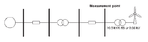
For a better appreciation of the points related to the harmonic signature of type 3 and type 4 WTGs that were discussed in the accompanying paper, measurements obtained at the HV side of the turbine transformer for the type 3 and type 4 turbines are discussed in this section. Measurements were conducted according to the existing version of the IEC 61400-21 standard [10]. The schematic diagram of the system used for the measurements and corresponding measurement point is shown in Fig. 1. The measurements were carried out on a single wind turbine. For both type 3 and type 4 turbines under consideration, the turbine transformer HV side is rated at 10.5 kV, whereas the transformer low voltage side voltage is 690 and 650 V for the type 3 and type 4 wind turbines, respectively. For different cases, wind turbines are connected to different power systems with different nominal voltages. The grid transformer voltage levels are not therefore shown in the figure. The short-circuit apparent power at the HV side of the grid transformer varies between 75 and 115 MVA for different grid conditions.
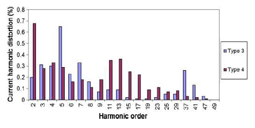
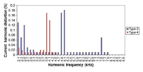
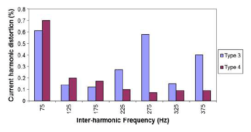
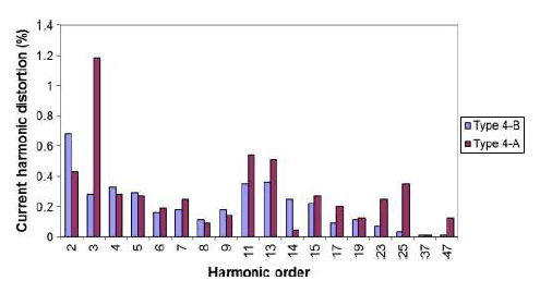


Figs. 2–7 show the harmonic current spectrum of type 3 and type 4 turbines for different frequency ranges of interest. A pessimistic assumption is taken here where the largest individual harmonics for different turbine loading conditions are stated in the same figure. In reality, all the largest individual harmonic currents cannot occur simultaneously. The total harmonic distortion measured in practice is therefore generally lower than that calculated from these figures unless a resonance condition occurs.
Common traits observed from the inspection of these figures are as follows.
1) Dominant low order noncharacteristic harmonics as shown in Fig. 2. For the type 3 turbine, the 5th and 7th harmonics have the largest magnitude, whereas the 2nd, 11th, and 13th are the largest for the type 4 turbine. These harmonics are noncharacteristic because they are not generated by the pulse width modulation (PWM) switching mechanism but introduced due to the interaction of WTG with the source power system. The presence of these low order harmonics depends on the background harmonics of the source power system and the application of harmonic cancellation techniques which will be discussed later in this paper.
2) High order harmonics associated with the PWM switching and its multiples. For the type 3 turbine, the most significant components include the 49th and 51st orders. The 39th and 41st orders are the largest for the type 4 turbine. Note that these harmonic are dependent on the converter switching frequency which may vary from one turbine type to another or even between two different turbines of the same type. No generic or general conclusions can therefore be made with respect to the largest high frequency harmonic current components. It is, however, understood that the most dominant switching harmonics are in the range of 2–10 kHz.
3) Zero-sequence triplen harmonics including the 3rd, 9th, and 15th could appear due to an asymmetry in the voltage of the medium voltage (MV) grid. For the type 3 and type 4 turbines discussed in Figs. 2–4, the zero-sequence triplen harmonics are within the acceptable range. Significantly high level of harmonic currents could occur if the WTG is connected to a weak and unbalanced source power system with some level of background triplen harmonic voltage. Note that this excessive harmonic distortion is not generated by theWTG, but it is the contribution of the grid which is measured at the WTG terminals. An example is shown in Fig. 5 for the type 4 turbine. In the figure system, conditions A and B indicate connection to a highly unbalanced and a relatively balanced source power system, respectively. Such high level of low order harmonic currents can be mitigated by various harmonic mitigation methods that will be explained later in this paper. Note that WTGs are generally connected to the MV grid via a star–delta connected transformer. The use of delta winding at the high side avoids the transfer of zero-sequence triplen components at the high side under balanced operating conditions. The zero-sequence components can, however, flow in the star winding unless the neutral point is not connected to the earth.
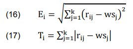
4) Inspection of Fig. 4 which depicts the dominant interharmonic current components reveals that, at certain cases, the magnitude of interharmonic currents can be larger than that of the integer harmonic currents. The interharmonics shown are arranged in subgroups, each covering a 50-Hz window from 75 to 375 Hz. For both type 3 and type 4 turbines, the largest interharmonic current is the 75-Hz subgroup which has a comparable magnitude to the most significant integer harmonic current components as shown in Fig. 2. In VSCs, interharmonic current components are generally produced when operating the two converters of a back-to-back system at different frequencies [11] or when connected to an unbalanced system [12]. In general, VSCs exhibit lower level of interharmonic currents compared to the line- or load-commutated converters due to the presence of an intermediate dc-link capacitor. Compared to a dc-link inductor, the capacitor acts as a filter for interharmonic components that tends to transfer from one converter to another. For a WTG, the operating frequency of the rotor-side converter is not generally constant but varies as a function of wind speed. During wind pattern changes, WTGs can therefore be a source of interharmonic currents.
5) As demonstrated in Figs. 5 and 6, the harmonic currents measured at the WTG terminals cannot be assumed constant. Fig. 5 shows the harmonic currents of a type 4 turbine when connected to two different source power systems, e.g., systems A and B. Fig. 5 shows the harmonic current injection of two type 3 turbines with similar control strategy but different ratings when connected to two different source power systems, e.g., systems C and D. These figures indicate the need for conducting harmonic measurements for each particular wind power plant. In the absence of such measurements, the largest values of individual harmonic currents can be taken, but this can give rise to the unnecessary design of harmonic filters at some circumstances. As will be demonstrated by practical case studies in Section III, this does not often give rise to a problem. This is because, in most cases, the individual and total harmonic components of the WPPs are well within the statutory limits except during resonance conditions.
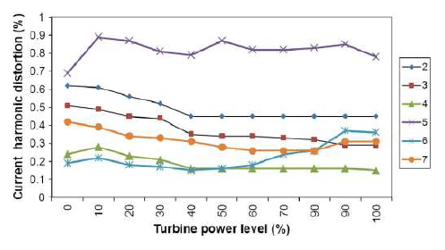
6) Figs. 7 and 8 illustrate the variation of harmonic current distortion as a function of wind turbine loading. No obvious trend can be deduced from these figures with respect to the variation of individual harmonics or the variation of the ratio of two individual components. This is because the variation of the harmonic currents as a function of turbine loading is stochastic. Despite this stochastic behavior, the variation of harmonic currents with respect to the turbine loading is marginal except for the 2nd harmonic component for the type 4 wind turbine. If harmonic measurements are carried out on-site for a range of turbine loading, the resulting harmonic current injection can be entered in a harmonic power flow simulation tool. In the absence of such data, this stochastic behavior can be neglected with constant harmonic current injection applied in all cases.
As shown in Figs. 7 and 8, several harmonic orders are larger when operating a type 3 or type 4 WTG at partial power. This does not, however, imply that a partial power operation is considered as more onerous from the grid harmonic distortion standpoint. This is because the values provided here are in percentage; a low power production will give rise to a lower distortion in ampere in many cases compared to the full power operation.
Another conclusion that can be drawn from these figures is that, in all cases except for the 2nd harmonic variations for the type 4 turbines, the harmonic distortion remains practically constant when operating at 60% loading and above. More distinct variations can be observed at light load operation.
Inspection of Figs. 2–6 indicates similar harmonic performance for type 3 and type 4 wind turbines. This is because both turbine types use PWM switched back-to-back VSCs with comparable switching frequencies. The main differentiator between the harmonic performance of type 3 and type 4 wind turbines arises from the way that the electrical generator is connected to the grid. With type 3 turbines, the electrical machine is not fully decoupled from the grid. Low order harmonics generated by the machine such as slip harmonics and slot harmonics are therefore reflected at the wind turbine terminals. Such harmonics are not relevant for type 4 wind turbines due to the full decoupling of the machine side and grid side and the fact that, with type 4 turbines, the machine slip is zero.
III. CASE STUDIES
This section discusses the harmonic performance of type 3 and type 4 turbines for both resonance and nonresonance conditions. Depending on the location of the installation, either IEC or IEEE standards are used. Power system studies reported in this section were carried out with DIgSILENT Power Factory simulation tool which allows the user to enter the magnitude and phase angle of the measured harmonic and interharmonic current components. Both balanced and unbalanced scenarios can be investigated. Additionally, the phase cancellation of corresponding harmonic components is accounted for using the IEC second summation law [13].
A. Nonresonance Conditions
This case study discusses a typical situation which usually occurs in WPPs where the harmonic distortion at various bus bars is within the statutory limits without the need for harmonic filters. This WPP uses type 3 turbines. Fig. 9 shows that the simulated voltage harmonic distortion reduces at the point of common coupling (PCC) as more capacitor banks are energized.

The total harmonic voltage distortion is well below the maximum limit for all cases. Distortion at the 46th harmonic is marginally higher than the IEC limit due to a grid resonance point around the 43rd harmonic as shown in Fig. 10. This is not, however, expected to cause any equipment malfunctioning, and no harmonic mitigation method is necessary in this case for the following reasons.
1) The long-term thermal effect of harmonics is evaluated for the sum of all harmonic components. Any potential thermal impact that can be caused by one harmonic component exceeding the permissible level will be compensated by the fact that all other harmonics and the total harmonic distortion are well within the statutory limits.
2) The only case where the planning levels of IEC 61400- 3-6 are exceeded is for operation at zero reactive power which is a very occasional operating point given the reactive power requirements of the particular wind power plant.
3) The likelihood of other system components injecting the 46th harmonic component is very low. System wide impact of the 46th harmonic is therefore negligible.
In this practical example, the WPP is therefore allowed to have a higher harmonic allocation for the 46th harmonic so long as it does not cause the network operator to breach its obligations in terms of harmonic management.
Fig. 11 shows the variation of the harmonic voltage distortion as a function of the level of the reactive power compensation. This figure indicates that the calculated harmonic voltage distortion for the 6th order harmonic marginally exceeds the IEC limit for higher level of reactive power compensation. These levels are unlikely to cause any equipment malfunctioning on the WPP itself and will have negligible effect on the PCC. They can be readily reduced by tuning the reactive power compensation capacitors; however, it is not necessary in this particular case for the following reasons.
1) Although the level of the 6th harmonic exceeds the planning level of IEC 61400-3-6, it is within the compatibility level of this standard which is 0.5%.
2) The long-term thermal effect of harmonics is evaluated for the sum of all harmonic components. Any potential thermal impact that can be caused by one harmonic component exceeding the permissible level will be compensated by the fact that all other harmonics and the total harmonic distortion are well within the statutory limits.
3) The harmonic compliance is assessed at the PCC rather than the collector grid.
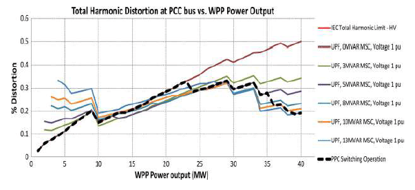
Fig. 12 shows the changes in total harmonic distortion at the PCC as a function of the WPP’s active power variation. In this case, the IEC specified limit of 3% is not shown as it lies off the top edge of the plot. This plot shows that the worst case total harmonic distortion at the PCC will be around 0.5% which is significantly lower than the IEC limit.
B. Resonance Caused by Grid Capacitor Bank With Type 3 Turbine
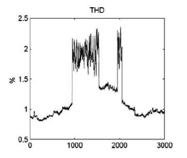
As discussed earlier, the harmonic signature of VSC-based wind turbines is generally insignificant. When a harmonic frequency coincides with one of the network resonance frequencies, a harmonic resonance can occur. This results in the amplification of the harmonic currents and voltages. A low harmonic current injection from the WTG can therefore be seen as a high harmonic voltage distortion at the PCC. Harmonic currents tend to flow from the harmonic generating sources to the lowest impedance seen. The lowest impedance is normally provided by the reactive power compensation capacitors. The installation of capacitors will shift the resonance point to lower frequencies. When coinciding with one of the dominant harmonics, a parallel resonance can occur. A practical example of harmonic resonance due to the use of plain mechanically switched capacitor (MSC) banks at the collector grid of the WPP with type 3 turbines is discussed here. The trace of the total harmonic voltage distortion as measured in practice is shown in Fig. 13. Results obtained from field measurements during the actual operation of this wind power plant indicate five distinct operating conditions as given in the following:
1) from 0 to 1000 s: no MSC;
2) from 1000 to 1500 s: one MSC;
3) from 1500 to 2000 s: two MSCs;
4) from 2000 to 2100 s: one MSC;
5) from 2100 to 3000 s: no MSC.
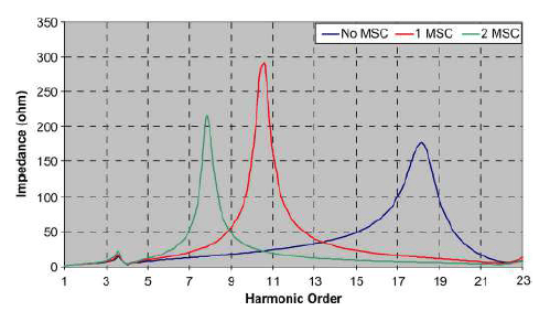
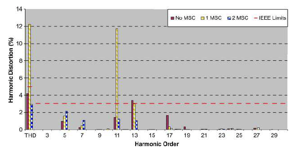
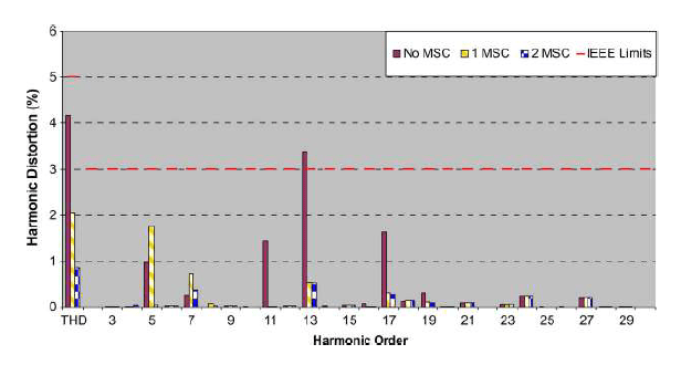
Results obtained from harmonic impedance scan and harmonic penetration studies are shown in Figs. 14 and 15, respectively. The harmonic impedance scan reveals a high impedance at around the 11th harmonic when one MSC is installed. As the 11th harmonic is also generated by the WTGs, the 11th harmonic and the total harmonic distortion can be as high as 12% as shown in Fig. 15. With two MSCs in service or without any MSC at all, the peak resonance point lies approximately around the 8th and the 18th harmonic order, respectively. These operating points will give rise to an acceptable level of harmonic distortion as confirmed by Fig. 15. This is because the WTG does not produce any appreciable level of the 8th and 18th harmonics. The mitigation method applied in practice to resolve the high total harmonic distortion (THD) problems is discussed in the next section.
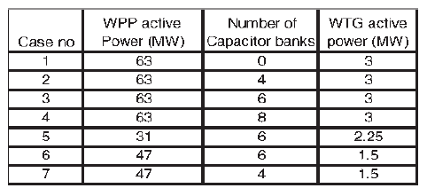
TABLE I – VARIOUS WPP OPERATING MODES CONSIDERED
C. Resonance Caused by Grid Capacitor Bank With Type 4 Turbine
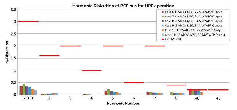
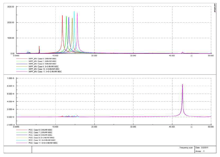
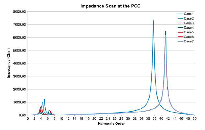
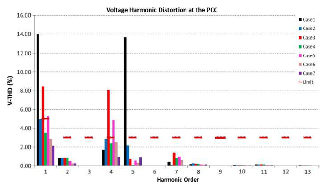
This case study discusses the possibility of harmonic resonance in a WPP utilizing type 4 turbines and proposes appropriate operating modes to avoid such a resonance. The operating modes investigated in terms of the WPP active and reactive powers are summarized in Table I where the size of each capacitor bank is 2.7 Mvar. The impedance scan and harmonic penetration studies for all cases looking at the PCC are shown in Figs. 16 and 17. From the impedance scan, two dominant peaks are visible: one at the lower order frequencies (3rd–7th order harmonics) and the other at higher frequencies (37th–44th order harmonics). The impedance scan for the lower order has a more pronounced impact as WTGs generate relatively higher harmonic current for those harmonics. The total harmonic voltage distortion at the PCC is primarily due to the 3rd–7th order harmonics. A closer inspection of the voltage harmonic distortion for the lower order harmonics is shown in Fig. 18.
Fig. 18 indicates that the total harmonic voltage distortion at the PCC exceeds the IEEE 519 standard voltage harmonic limits when there are no or six capacitor banks in service. Pertinent mitigation methods would be necessary to maintain the harmonic within the IEEE 519 standard limit. With four and eight capacitor banks, the voltage harmonic distortion is within the limits due to a shift in the resonance frequency away from the 4th and 5th harmonics. The WTG injects these harmonic currents, and if a resonance point is close to these harmonic frequencies, a harmonic voltage amplification will occur.
The three case studies presented in this section have demonstrated that a low harmonic current at the wind turbine terminals can give rise to a low or high harmonic voltage profile at the grid. A direct relationship cannot therefore be established between the harmonic currents at the wind turbine terminals and harmonic voltage at the collector grid or at the point of common coupling. The main factors determining the harmonic voltage profile are the network impedance and the presence of background harmonic voltages at the grid.
IV. HARMONIC MITIGATION
In general, the harmonic distortion of WPPs can be managed by the use of active and passive harmonic filters, the use of multilevel converters in wind turbines instead of the commonly used two-level converters, the use of selective harmonic elimination (SHE) modulation strategy, the use of converter control for harmonic compensation, and third harmonic current injection [14]. The most common methods applied to modern wind turbines are classified into the turbine- and system-level mitigation methods as discussed in this section. One important consideration in designing passive harmonic filters is that, while they are effective in the mitigation of the certain harmonic order(s), they could give rise to the amplification of some other harmonics if not carefully deigned.
A. Harmonic Filtering
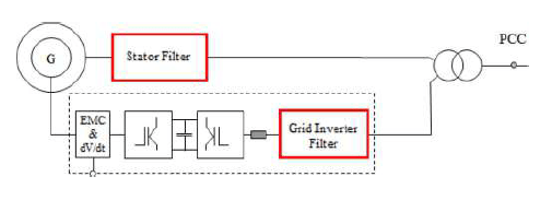
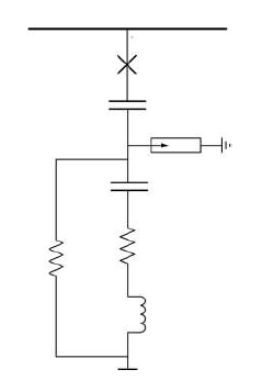
1) Turbine Level Filtering: Most commercial wind turbines utilize VSCs at both the grid- and rotor-side converters for both type 3 and type 4 turbines. The modulation of these converters gives rise to the generation of harmonics at both the gridand rotor-side converters. The resulting harmonics are therefore generally dealt with by the installation of the harmonic filters at both the grid- and rotor-side converters. The schematic diagram of the required filter for a type 3 wind turbine is shown in Fig. 19. Note that the high-frequency electromagnetic compatibility choke and dv/dt filters are also utilized as the machine terminals to deal with the zero-sequence common mode voltage and currents which practically eliminate the shaft bearing currents. These filters are not explicitly discussed from a harmonic study standpoint as they are not effective for the frequency range of harmonic studies.
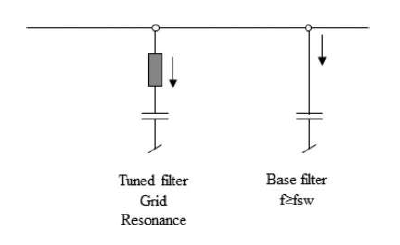
An example demonstrating the constituting components of the grid-inverter-side harmonic filter is shown in Fig. 20. This figure shows that the filter comprises the following two branches:
1) a tuned LC circuit for damping resonance with the transformer and the grid inductance; 2) a base filter for damping of the switching frequency and its multiples;

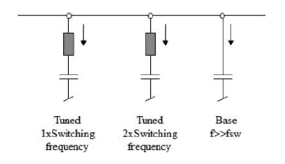
As shown in Fig. 21, the stator-side filter consists of the three following branches:
1) a tuned LC circuit for damping the switching frequency;
2) a tuned LC circuit for damping twice the switching frequency;
3) a base filter for multiples of the switching frequency.
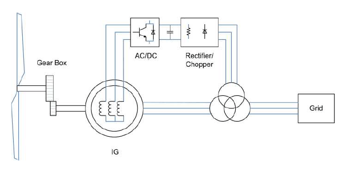
Note that a variation of the conventional type 3 turbines sometimes implemented in practice does not include any active PWM converter as shown in Fig. 22. For this design of type 3 turbine, a stator-side harmonic filter is not therefore necessary.
2) System Level Filtering: The system level mitigation techniques generally deal with the harmonic resonance aspect rather than the harmonic emission aspect. These methods generally aim to avoid any harmonic resonance issue which can cause a dangerously high level of harmonics even for an acceptable level of harmonic injection from the WTGs. A simple way to avoid the harmonic resonance issues is to tune the resistive and the inductive part of the capacitor. For the system discussed in Section III-B, this can be achieved by converting the existing capacitor banks to the 11th and 5th harmonic filter banks. Each branch of such a filter is schematically shown in Fig. 23. The methodology to derive the R, L, and C parameters is discussed in detail in [15].
Simulation results obtained from the harmonic penetration studies indicate that, with an 11th harmonic filter bank, the THD reduces to 2% from the 12%, mainly due to the filtering of the 11th harmonic. With the 11th and 5th harmonic filter banks, the THD reduced further to 0.9% due to the filtering of the 5th harmonic. As shown in Fig. 24, with the use of tuned filters, the harmonic distortion limits during operation with one or two capacitor banks are maintained within the limit specified by the IEEE Std 519 for the voltage levels between 69 and 161 kV. Alternatively, a C-type harmonic filter can be employed. In a C-type filter, an auxiliary capacitor is connected in series with the reactor as shown in Fig. 25. The auxiliary capacitor is smaller than the main capacitor. The reactor and auxiliary capacitor are chosen to form a series resonance at the fundamental frequency. The impedance of the branch comprising the reactor and auxiliary capacitor is therefore zero. The damping resistor is practically short-circuited at the fundamental frequency, and a C-type filter produces negligible fundamental frequency losses. The reactive power rating of the filter is determined by the main capacitor only.
B. Harmonic Compensation
Passive harmonic filters are generally effective in mitigating harmonic current emissions emanated from the WTGs. They are not, however, effective in dealing with systems with appreciable levels of background harmonic voltages. For these conditions, a harmonic compensation method can be adopted. In a harmonic compensation method, no actual damping resistance is used, but the energy is stored in the dc-link capacitance of the back-to-back converter. The energy dissipation is therefore significantly lower than that with a passive damping resistor. The main objective of the harmonic compensation is to reduce the harmonic currents generated by the generator due to the stator and rotor windings and to mitigate the background harmonic voltage. Nonlinearities in the stator and rotor windings results in harmonics in the stator currents. As shown in Fig. 2 for a type 3 turbine, the 5th and 7th harmonics are the most significant orders. For a type 3 turbine, the harmonic content in the rotor voltage gives rise to slip-harmonic frequencies in the stator currents. A grid harmonic compensation reduces the amplitude of the harmonic content in the line currents by using the grid converter to make harmonic currents in opposite phase angle to the harmonic currents on the stator. Note that slip harmonics generally fall in the category of the interharmonic for which more stringent limits are imposed. The grid harmonic compensation can be superimposed on the grid current controller using a summation junction. The overall design should be such that the grid current control performance remains unchanged with and without the grid harmonic compensation. Considering that the most significant harmonics for a type 3 turbine are the 5th and 7th orders, the harmonic frequencies can be calculated by (1) and (2)

where
n = 1, 2, 3, . . .;
m = 1, 2, 3, . . .;
fh hth harmonic frequency;
fsh hth slip-harmonic frequency.
Considering the first slip harmonic, this is simplified to
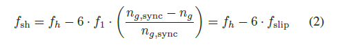
where generator speed; ng,sync synchronous generator speed.
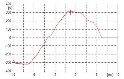
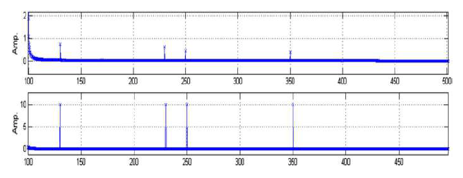
The effectiveness of the harmonic compensation using the grid harmonic damping is illustrated in Fig. 26 for a type 3 turbine. In the figure, the upper and lower graphs correspond to those with and without harmonic compensation, respectively.
The harmonic compensation method described earlier can be used independently or along with a SHE modulation strategy which also aims at mitigating the low order harmonics. The discussion provided in this section has mainly focused on the type 3 turbine. The same principles hold true for a type 4 turbine except that no compensation is required for the slip harmonics.
V. CONCLUSION
This paper discussed practical experiences and mitigation methods of harmonics in wind power plants. The harmonic signature of practical type 3 and type 4 turbines was first presented. It was shown that VSC-based WTG can generate an appreciable level of low order harmonics and interharmonics in addition to the high order switching harmonics. As these low order harmonics are to a large extent generated by the interaction with the source power system, results obtained from different measurements can reveal different levels of harmonic currents and voltages. The impact of turbine loading condition was observed, but it was perceived to be marginal.
Simulation results obtained from conducting power system harmonic studies on practical WPPs are presented. For the nonresonant conditions, the magnitude of harmonics is significantly lower than the statutory limits. Resonances excited by the grid capacitor bank for WPPs using type 3 and type 4 turbines were investigated, and pertinent mitigation methods applied in practice were highlighted.
Different mitigation methods applied in practical WPPs were discussed. This includes turbine- and system-level mitigation techniques. In general, passive filters at the system level and/or the turbine level are employed. The use of harmonic compensation at the turbine level provides an active mechanism to deal with the low order harmonics and interharmonics, therefore avoiding the risk of resonances internally at the turbine or externally with the interconnected network.
REFERENCES
[1] B. Badrzadeh, M. Gupta, N. Singh, A. Petersson, L. Max, and M. Høgdahl, “Power system harmonic analysis in wind power plants—Part I: Study methodology and techniques,” in Conf. Rec. IEEE IAS Annu. Meeting, Las Vegas, NV, USA, Oct. 2012, pp. 1–11.
[2] S. Liang, Q. Hu, and W.-J. Lee, “A survey of harmonic emissions of a commercial wind farm,” in Proc. IEEE Ind. Commercial Power Syst. Tech. Conf., Tallahassee, FL, USA, May 2010, pp. 1–8.
[3] L. H. Kocewiak, J. Hjerrild, and C. Leth Bak, “Harmonic generation and mitigation by full-scale wind turbines: Measurements and simulation,” in Proc 10th Int. Workshop Large-Scale Integr. WindPower Power Syst./Transmiss. Netw. Offshore Wind Power Plants, Aarhus, Denmark, Oct. 2011, pp. 1–8.
[4] K.-D. Dettmann, S. Schostan, and D. Schulz, “Wind turbine harmonics caused by unbalanced grid currents,” in Proc 7th Compat. Power Electron., Gdansk, Poland, May/Jun. 2007, pp. 1–6.
[5] L. H. Kocewiak, J. Hjerrild, and C. Leth Bak, “The impact of harmonics calculation methods on power quality assessment in wind farms,” in Proc 14th Int. Conf. Harmon. Qual. Power, Bergamo, Italy, Sep. 2010, pp. 1–9.
[6] L. H. Kocewiak, J. Hjerrild, and C. Leth Bak, “Wind farm structures’ impact on harmonic emission and grid interaction,” in Proc. Eur. Wind Energy Conf., Warsaw, Poland, Apr. 2010.
[7] K. Yang, M. H. J. Bollen, and M. Wahlberg, “A comparison study of harmonic emission measurements in four wind parks,” in Proc. IEEE Power Energy Soc. Gen. Meeting, San Diego, CA, USA, Jul. 2011, pp. 1–7.
[8] M. H. J. Bollen, L. Yao, S. K. Roonberg, and M. Wahlberg, “Harmonic and interharmonic distortion due to a windpark,” in Proc. IEEE Power Energy Soc. Gen. Meeting, Minneapolis, MN, USA, Jul. 2010, pp. 1–6.
[9] L. Sainz, J. J. Mesas, R. Teodoresu, and P. Rodriguez, “Deterministic and stochastic study of wind farm harmonic currents,” IEEE Trans. Energy Convers., vol. 25, no. 4, pp. 1071–1080, Dec. 2010.
[10] Wind Turbines—Part 21: Measurement and Assessment of Power Quality Characteristics of Grid Connected Wind Turbines, IEC Std. 61400-21, 2008.
[11] J. Song-Manguelle, S. Schroder, T. Geyer, G. Ekemb, and J. M. Nyobe- Yome, “Prediction of mechanical shaft failures due to pulsating torques of variable frequency drives,” IEEE Trans. Ind. Appl., vol. 46, no. 5, pp. 1979–1988, Sep./Oct. 2010.
[12] M. R. Rifai and T. H. Ortmeyer, “Evaluation of current interharmonics from ac drives,” IEEE Trans. Power Del., vol. 15, no. 3, pp. 1094–1098, Jul. 2000.
[13] Electromagnetic Compatibility (EMC)—Part 3-6—Limits: Assessment of the Connection of the Distorting Installation to MV, HV and EHV Power Systems, IEC Std. 61000-3-6, 2008.
[14] D. G. Holmes and T. A. Lipo, Pulse Width Modulation for Power Converters: Principles and Practices. London, U.K.: Wiley, 2003.
[15] B. Badrzadeh, K. S. Smith, and R. C. Wilson, “Designing passive harmonic filters for an aluminum smelting plant,” IEEE Trans. Ind. Appl., vol. 47, no. 2, pp. 973–983, Mar./Apr. 2011.
Authors: Babak Badrzadeh (S’03–M’07–SM’12) received the B.Sc. and M.Sc. degrees from Iran University of Science and Technology, Tehran, Iran, in 1999 and 2002, respectively, and the Ph.D. degree in the area of electrical power engineering from Robert Gordon University, Aberdeen, U.K., in 2007. After spending a short period as an Assistant Professor at the Technical University of Denmark, Lyngby, Denmark, he joined Mott MacDonald, Transmission and Distribution Division, U.K., as a System Analysis and Network Planning Engineer. From March 2010 to March 2012, he was with Plant Power Systems, Vestas Technology R&D, Aarhus, Denmark, where he acted as a Lead Engineer in the area of advanced wind power plant simulation and analysis. Since May 2012, he has been with the Australian Energy Market Operator, Melbourne, Australia, as a Network Models Specialist. His areas of interest include power system electromechanical and electromagnetic transients, application of power electronics in power systems, wind power plants, and modeling and simulation.
Manoj Gupta received the M.Tech. degree in power systems from the Indian Institute of Technology, Kanpur, India, in 1996. He has over 15 years of experience in power system analysis and modeling. He has worked with ABB in India and Germany and Mott MacDonald in the U.K. He is currently working with Vestas in Singapore, where he leads a team for wind power plant interconnection and grid code compliance studies. His areas of interest are power system analysis and modeling for renewable, oil, and gas, industrial plants, protection, and distribution network planning.
Source & Publisher Item Identifier: https://www.downloadmaghaleh.com/wp-content/uploads/edd/maghaleh/1398/soltani.harmonik-mazare-badi_compressed.pdf, Digital Object Identifier 10.1109/TIA.2013.2260314