Power Quality Blog

Accurate Fault Detection and Location in Power Transmission Line Using Concurrent Neuro Fuzzy Technique

Published by Patrick S. Pouabe Eboule, & Ali N. Hasan, University of Johannesburg, South Africa

Abstract. In this paper a new approach for the detecting and locating different kinds of faults on power transmission lines using the concurrent neurofuzzy technique (CNF) is introduced. This approach relies on the advantages of combining fuzzy logic (FL) and the artificial neural network (ANN) to detect, classify and locate faults on a power transmission line that carries high voltage and very high voltage of 400 kV and 750 kV respectively over short distance and long distance of 120 km and 600 km respectively. Results exhibit that CNF is capable of detecting several and different fault types and locations with high accuracy, which will reduce the time for the technical team maintenance to achieve their goals.

Streszczenie. Wartykule przedstawiono nowe podej´scie do wykrywania i lokalizowania ró˙znego rodzaju usterek w liniach elektroenergetycznych przy u˙zyciu współbie˙znej techniki neuro-rozmytej (CNF). Podejs´cie to opiera sie˛ na zaletach poła˛czenia logiki rozmytej i sztucznej sieci neuronowej w celu wykrywania, klasyfikowania i lokalizowania usterek w linii elektroenergetycznej, która przenosi wysokie napi˛ecie i bardzo wysokie napi˛ecie odpowiednio 400 kV i 750 kV w krótkim czasie odległos´c´ i długa odległos´c´ odpowiednio 120 km i 600 km. Wyniki pokazuja˛, z˙e CNF jest w stanie wykryc´ kilka róz˙nych typów usterek i lokalizacji z duz˙a˛ dokładnos´cia˛, co skróci czas potrzebny zespołowi technicznemu na osia˛gnie˛cie celów. (Precyzyjne wykrywanie i lokalizowanie usterek w linii przesyłowej energii przy u˙zyciu równoległej techniki neuro-rozmytej)

Keywords: Transmission Line Systems, Fault Detection, Fault Location, Concurrent Neuro-Fuzzy Technique
Słowa kluczowe: Systemy linii przesyłowych, Wykrywanie uszkodze´ n, Lokalizacja usterki, Równoczesna technika neuro-rozmyta

Introduction

The first AC power transmission line system was initially introduced in the year 1889 in the United States of America [1]. The first electrical transmission line was connected between Oregon city and Portland. This line was characterized by a line voltage of 4 kV, single phase with a length of 21 km. However, the first three-phase system was introduced and built in Germany in 1891. The transmission line covered a distance of 179 km at 12 kV[1].

AC power transmission line systems have been researched and improved since it was first introduced. Powerful transmission line systems have been implemented and installed all over the world to meet the ever growing energy demand over the years. Nowadays, we are able to transmit electrical energy at various distances using modern and sophisticated power transmission systems. However, these sophisticated energy transmission systems come with limitations and challenges. Therefore, there is need to continuously monitored and maintained the power transmission lines in order to eliminate catastrophic breakdown and disruption of services to the end user costumers[2, 3, 4].

Several techniques and approaches have been developed by various researchers for troubleshooting and detecting faults in transmission power lines. These techniques include discrete Walsh-Hadamard transform, discrete wavelet transform, naive bayes classifier, hilbert huang transform and k-means data description method. However, these techniques come with limitations and did not perform optimally when applied for detecting and locating faults.[5, 6, 7, 8, 9, 10].

In 2020, Aker et al. used wavelet transform and naive bayes classifier to identify the type of fault that may occur in the shunt compensated static synchronous compensator. The network was designed using Simulink and faults were applied at disparate zones. The technique decomposed the obtained waveforms into several levels using Daubechies mother wavelet and applied naive bayes to classify the faults. It emerged from this study that the accuracy could be up to 80%. However, only fault classification was implemented [5].

Earlier in 2019, Kapoor applied a discrete Walsh- Hadamard transform to detect faults and identified faulty phase in a three phase transmission line connected with distributed generation. In this technique, the fault data was recorded using characteristics based on Walsh-Hadamard coefficients of the current. It emerged from this research that the method can effectively identify the fault phase [8, 9]. The same year, Hosein et al. proposed and applied ANFIS technique for detecting faults in smart grids. The currents measured at only one side of a three-phase transmission line is collected and passed through a signal processing module. The results obtained are compared against other AI techniques (ANN and SVR). It emerged from this study that the best accuracy obtained is 87.5% for ANFIS technique which outperforms SVR and ANN techniques. However, this paper only dealt with faults location and did not propose faults classification. Moreover, only four different fault types were considered in obtaining the total dataset. The total accuracy obtained could have been improved on this case studied by increasing the size of the dataset [11].

As the transmission line grid continuously grows with the increasing demand on energy, it becomes more complex and difficult to prevent faults from occurring. Therefore, the convectional methods of troubleshooting and detecting faults in transmission lines are becoming inefficient and obsolete. Thus, the need to develop and implement new techniques that can accelerate the process of fault detecting and also ensure a good compatibility of the modern and complex electrical system is necessary [12]. In addition, the current methods of fault detection also suffer from a reliability problem because faults on transmission lines are often non-linear that is to say, there is no formal causal effect relationship between the detected fault and its origin. Therefore, these methods are unable to solve non-linear problems [13].

As a result, it was essential to develop an intelligent system that can predict, detect and locate different fault types. These fault detection systems use artificial intelligence techniques.

Power transmission lines are subject to multiple defects [14, 12, 15]. These faults and defects can be subdivided into different types of faults such as single line to ground fault (SLG), double line to ground fault (DLG), triple line fault (TL) and triple line to ground fault (TLG) [14, 12, 15, 16]. The most frequent fault that occurs on power transmission lines is the over-voltage fault, which comes from capricious atmospheric conditions such as lightning, bush fires and cyclones [17, 18]. These faults have a damaging and hazardous impact on the transmission lines and the power system in general [17].

Artificial Intelligence (AI) fault detection techniques have shown to be more accurate and more promising [19, 20, 21, 22]. Researchers have found a more robust approach and solution in solving complex problems by using different combinations of these AI techniques [23, 24]. In power transmission lines, fault types are numerous and diverse. Thus, faults are distinguished based on the meteorological conditions from those of an electrical/mechanical origin, coming from the production system [16].

Climate change is one of the causes of faults on power transmission lines. It can affect a cable by accelerating its ageing process [17, 18]. The use of AI techniques could accelerate the process of detection, classification and location of the faults over long power transmission lines carrying high voltage electricity. A Concurrent Neuro-Fuzzy method was used in this experiment because it combines two powerful AI techniques of fuzzy logic (FL) and neural networks (ANN). These two methods, FL and ANN, have repeatedly and successfully been used in different fields of engineering to solve problems where the traditional and classical methods have not been able to provide genuine solutions [19, 23].

In 2018, Eboule et al. proposed a fault detection and location algorithm based on concurrent neuro fuzzy. The technique consisted of setting various FL conditions and of using ANN to process them in order to detect, classify and locate 11 fault types that may occur in transmission lines. It emerged from this study that the accuracy of an AI system is directly linked to the number of data sets and the architecture of the system [2, 4]. However, this paper only dealt with one type of transmission line and did not take all significant transmission line’s parameters into consideration.

In 2015, Anamika et al. improved the performance of a transmission line using a fuzzy inference system. The method consisted of designing three distinct systems respectively for transmission line directional relaying, fault classification and fault location schemes using fault current and voltage available at the relay location. It emerged from this study that the proposed method can efficiently detect faults for both forward and reverse directions [25].

In 2013, Marjan et al. [26] implemented a fault location algorithm that can be used to locate various faults along mixed line-cable transmission corridors based on the telegraph’s equations. It emerged from this study that the use of Clarke transformation is powerful when dealing with transient studies. In 2012, Carlo et al. in [3] used FL to classify various faults in single and double circuit lines. They concluded that to improve the yield of their system, FL membership functions have been chosen to have an overlap with each other. A modified technique was proposed to increase the accuracy and the performance of the proposed FL fault detection in double-circuit was tested using 3000 cases. Early in 2005 Mahmoud et al. studied in [27] a combined overhead line with underground cable for fault location. The simulation was done via Matlab and it emerged from this implementation that the maximum error in the overhead section was 0.21% over 100 km while underground the error was 1.643% over 10 km.

The limitation found in the above literature is that CNF is not widely used in various engineering fields. However, Eboule in [2, 4] introduced the use of the CNF technique for power transmission line faults detection and location in a limited scale. This paper provides in depth use of CNF technique for power transmission line fault detection and location taking into consideration all significant parameters of the transmission lines and with a bigger data set and information used in two experiments. The obtained results are compared to [2] paper results and [4] paper results.

The main objective of this work is to introduce and use the powerful artificial intelligence technique called CNF technique for the application of power transmission line fault detection and location. This will be achieved by following a well-defined and structured sequential methodological approach of CNF functions in detecting and locating faults for two distinct power transmission lines. Comparison analysis with the previous studies will also be investigated to determine the performance efficiency of the proposed CNF technique. The first transmission line is characterized by its voltage of 750 kV over 600 km distance while the second transmission line has 400 kV over 120 km distance. The impact of this study could lead to reduced power system and transmission line maintenance cost and time. This will result in sustainable power delivery to customers and increased grid reliability. This will increase the income of the company supplier and will help developing a great business environment which is necessary to absorb the level of unemployed.

This article put forward four main contributions. The first contribution is the implementation of a new technique (CNF) to detect, classify and locate power transmission line faults for high voltage and very high voltage over short and long line lengths. The second contribution is the application of such a technique into a system that includes 11 different fault types and take all significant power transmission line parameters into consideration and compare the obtained experimental results. Knowing that this concurrent neuro fuzzy technique has been applied in [23] on surface roughness modelling in drilling. The third contribution is to investigate if this AI technique could be effectively applied for fault detecting and locating for long transmission lines. Because the application of the technique in transmission line is still new, thus, the fourth contribution is to demonstrate the robustness of the technique and to make it be common.

This paper is organized as follows. Section 2 introduces the CNF technique, Section 3 describes the experiment setup, Section 4 discusses the experimental results obtained and Section 5 presents the conclusions.

Concurrent neuro fuzzy technique

In these experiments a methodology using CNF that deals with two tasks of detecting and locating faults on PTLs is introduced. Two different data sets were used for the two tasks of locating and identifying the faults. Therefore the CNF was trained separately twice with each data set.

The concurrent neuro-fuzzy (CNF) technique was introduced by Jang Lin and Lee in 1991. Since then, the CNF technique has been successfully applied in many fields and tasks such as control tasks, data analysis, detection and classification. The CNF technique generally represents a set of two distinct FL and ANN methods used to solve a precise problem where the FL method determines the rules and ANN adjusts these rules [23]. FL has been used in many applications. It has been successfully used in exploiting and processing the data in different areas such as image processing, image recognition in medicine and video surveillance. It has become apparent that the greatest challenges of this method is the determination of the rules and the search for the appropriate membership function to reduce the percentage of error [24, 28, 29]. This allowed for the introduction of the ANN technique in data processing to make the algorithm more efficient in the assigned task. CNF allows FL and ANN to analyze the data together and concurrently. Figure 1. presents the general architecture of the CNF network.

In Layer 1, the obtained data from the post faults are directly transmitted to the next layer.

where y_i⁽¹⁾represents the output of all neurons in Layer 1 and x_i⁽¹⁾ represents the input of Layer 1. In Layer 2, the fuzzification is applied. The membership function which was used is triangular sets and the two parameters, a and b, are determined as follows.

Where y_i⁽²⁾ is the output Layer 2, x_i⁽²⁾ is the input Layer 2 which is the X-axis in Figure 2 and a, b are parameters as follows in Figure 2.

In Layer 3, different fuzzy rules are defined. Intersection was implemented by the product operator as shown in Equation 2.

Where: y_i⁽³⁾ is the outputs of Layer 3 and x_ki⁽³⁾ is the input of the (k) neuron in Layer 3. In Layer 4, the consequence of FL rules is represented. CNF uses the probabilistic OR operation to determine the outputs of each neuron.

Where: y_i⁽⁴⁾ represents outputs of Layer 4 and x_ki⁽⁴⁾ is the inputs of the (k) neuron in Layer 4. In Layer 5, a single output of the neuro-fuzzy system was represented; it is the layer where defuzzification takes place. Output is computed by applying the sum product composite technique. Equation 4 presents how to compute the predicted output of the CNF network [23].

Fig.3. Power transmission line fault location

Table 1. Power transmission line parameters.

where, y represents the output of the neuro-fuzzy system and μ_ck is (k) output of the layer 4.

Experiment setup

The experiment was conducted on a three-phase power transmission line (PTL) as shown in Figure 3 using the line parameters in Table 1 of the South African main energy supplier (ESKOM Ltd). These PTLs have the same R, L, C parameters but, the line voltage and the length of the lines are different. The experiment was simulated using MATLAB/ SIMULINK. All 11 faults were set manually using a logical signal to control the fault operation as shown in Figure 4. the ground and the fault resistances were defined. The sampling frequency for the fault simulator was set at 0.2 to generate each fault sample data. A 2200 data sample (11 faults × 10 fault resistances × 5 zones × 4 fault angles) were generated and collected from the post-faults (short-circuit voltage and current) and used for training and testing the CNF network. This sampling frequency corresponds to the rate at which the system samples its inputs.

At different distance along the line, different fault types were simulated in terms of fault angles and fault resistances in order to have all different types of faults with their location where they occurred on the PTL. The short-circuit voltage and current were recorded at the beginning of the line and used as the inputs for the experiments.

Four experiments were conducted, the split percentages for the two data sets of the fault type and the fault location was 70% to train and 30% to test. The experiments were conducted using successively 550, 1100 and 2200 data as mentioned in Table 3. The first two experiments were for fault type detection for long and short transmission lines whereas the third and the fourth experiments were for fault location for long and short transmission lines.

For the fault detection experiment, the CNF network shown in Figure 1 with 5 hidden layers were used. In these experiments, the structure of the CNF method was determined using the standardized data of the post faults. The computation number of neurons for each layer in the CNF network follows a certain number of rules such as the number of the inputs, the number of the FL conditions and the membership function type [2, 30, 33]. Thus, the determination of the most accurate CNF network structure for power transmission line fault type detection is obtained.

For Layer 1, six neurons were used, these neurons correspond to the required six input variables V_a, V_b, V_c, I_a, I_b, I_c respectively. The six input variables represent the root mean square (RMS) of the short circuit voltage phase to ground and the short circuit current across the conductors A, B and C of the power transmission line. Data were normalized using the following normalization equation.

Where: X_n is the normalized data for each variable, X_min, and X_max are the minimum and the maximum values respectively.

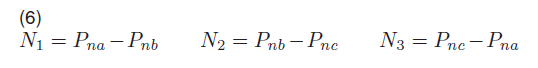
In Layer 1, the output dimension represents the six input variables times the number of faults (6×2200). In Layer 2, three conditions have been established for the CNF algorithm so that the determination of the number of neurons at this layer corresponds to the number of conditions of the FL multiplied by the number of inputs data [31, 32]. The number of neurons for Layer 2 is 6×3 = 18 neurons. The output dimension obtained was the number of neuron times the number of faults (18×2200).

The three required FL conditions are N₁,N₂ and N₃.

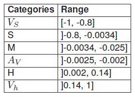
Table 2. Different ranges of the membership function

These conditions were determined as follow:

P_n parameters was found as follows:

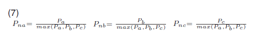
where:

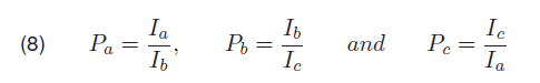
I_a, I_b and I_c are the post fault currents flowing in the A, B and C conductors of the transmission lines. The choice applied in Layer 2 was made according to the membership function of the data. For this experiment, a triangular membership function was used as shown in Figure 5, as soon as the the membership function categories with their values range obtained shown in Table 2.

Where: Very Small (V_S), Small (S), Medium (M), Average (A_V), High (H), Very High (V_h)

In Layer 3, each neuron corresponds to each fault type. Consequently, eleven neurons were necessary for 11 FL conditions [33]. The output dimension for this layer was obtained according to the number of FL conditions multiplied by the total number of data used (11 × 2200). In Layer 4, the number of membership functions is six which corresponds to the number of neurons.

Consequently, six neurons were necessary. The outputs of each neuron in this layer were determined by following the probabilistic OR approach and the dimension of the output in this layer is 6× 2200. In layer 5, the sum average of centroids technique was used to determine the output for the CNF network. It can be seen from Equation 8 that only current data were used to define and set the fuzzification rules. Usually one parameter is used in such experiment to set the FL rules in order to reduce the experiment computation time and complexity but the increasing of the input variables could reduced the obtained error [2]. The final output dimension obtained for fault classification is 1×2200. The different FL conditions used to set the CNF technique parameters are given below

• If N₁ is V_h and N₂ is H and N₃ is V_S then SLAG
• If N₁ is V_S and N₂ is V_h and N₃ is H then SLBG
• If N₁is H and N₂ is V_S and N₃ is V_h then SLCG
• If N₁ is V_S and N₂ is V_h and N₃ is M then DLAB

Fig.6. Flow chart of the fault detection and classification technique

Fig.7. Network structure for fault location

• If N₁ is V_Sand N₂ is H and N₃ is V_h then DLBC
• If N₁ is V_hand N₂ is VS and N₃ is S then DLAC
• If N₁ is V_S and N₂ is Vh and N₃ is A_V then DLABG
• If N₁ is V_S and N₂ is S and N₃ is V_h then DLBCG
• If N₁ is V_h and N₂ is S and N₃ is S then DLACG
• If N₁ is S and N₂ is S and N₃ is H then TLABC
• If N₁ is S and N₂ is S and N₃ is V_h then TLABCG

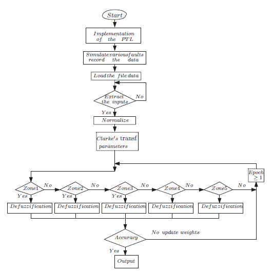
Two experiments (experiment 1 and experiment 2) were carried out using CNF network for two transmission lines fault type detection. Experiment 1 and 2 algorithm is shown in Figure 6 flow chart. The algorithm steps are explained as follows:

• Load the file data
• Extract the input data from the data file
• If the Extraction is successful, normalize the input data, else repeat the previous step
• Define the output data
• Normalize the output data
• Define the functionality of each neuron in all layers from layer 1 to layer 5
• If the previous step is successful, initialize weights, else repeat the previous step
• Determine error in each neuron
• Update weights between different neurons
• Define the number of epochs
• Train and Test the concurrent neuro-fuzzy structure

For experiments 3 and 4, the structure of CNF for faults location in both lines is shown in Figure 7.

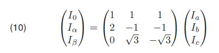
In these experiments, telegrapher’s equation was used to locate faults over power transmission lines. Telegrapher’s equation converts three phase lines to Clarke’s transformation to determine 0, alpha (α), and beta (β) variables [2, 34]. The utilization of Clarke’s transformation is recurrent in fault location because in PTL we have symmetrical and unsymmetrical faults. Three phase power transmission lines are presented in Figure 3 with a fault which occurs at l distance from the generation side.

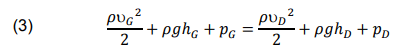
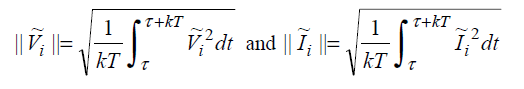
The voltages and currents for the three phase transmission lines are transformed using Clarke’s transformation as the following:

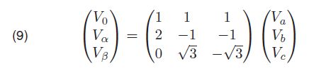
and

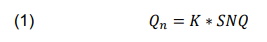
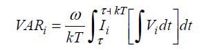
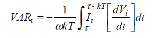
Thus, fault distance parameters can be computed as:

where i = 0, α, β
l_α and l_β are the two areal modes, l₀ is the ground mode. γ_i, Z_ci, Υ_i and Z_iare determined using the line parameters as shown in equation 12:

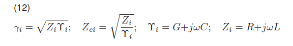
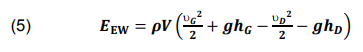
R, L, G and C are the lines parameters, the resistance, the inductance, the conductance and the capacitance respectively. A_i and B_i are determined using the line voltages, the line distance and the line impedance as shown in equations 13 and 14

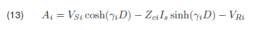
and

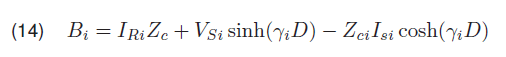
An accurate fault location point can be determined by the appropriate mode 0, alpha, and beta. V_S is voltage sending, V_R is voltage received, D is total length of the line,

l_α is valid for all types of fault except line to line faults where the l_β is applied.

The outputs from Layer 1 to Layer 5 have a 2200×6 dimension. However, after the data were split into 0, α and β variables respectively, the dimension outputs obtained in layer 5 were 600×1, 600×1 and 1000×1. The CNF algorithm for fault location is programmed by using Matlab software. Flow chart of the CNF algorithm for faults location is illustrated in Figure 8 and the proposed algorithm works as follows:

Fig.8. Flow chart of the fault Location technique

• Load data
• Define variable
• Layer 1 normalise input data and forward to Layer 2
• Layer 2 divide data to 0, α and β data
• Layer 3 apply Clarke’s transformation
• Layer 4 determine parameters transmitted (voltage and current)
• Layer 5 determine output distances
• Initialise weights, Determine error in each neuron
• Update weight in different neurons for each layer
• Define the number of epochs, Train and Test the system

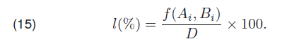
Most important in error calculation is magnitude [35, 36, 37]. Thus values of error were determined for fault location using equation 16 .

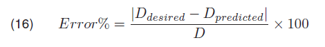
where D_desired represents the fault distance desired, D_predicted the fault distance is determined using the algorithm and D the total length of the line.

Experiment Results and Discussion

Experimental results show that the best and most accurate results are obtained when using the 2200 data set as shown in Table 3. For this fault classification experiment, the number of neurons that characterize the topology of the CNF structure was determined according to FL rules. Thus, the structure of the CNF algorithm for the detection and classification of faults was the same for both transmission line short and long length which is 6-18-11-6-1.

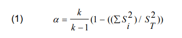
The evaluation error was obtained by summing the various input data which do not satisfy the conditions established by FL and dividing this sum by the total number of data inputs. Therefore, the total achieved fault type prediction accuracy is approximately 97.5% for the long line and 95.6% for the short line.

Table 3. Fault location prediction results.

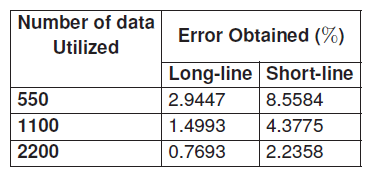
Table 4. CNF fault defuzzication output and FL conditions for the long line at 600 km, R_f = 0.001 Ω, fault angle = -2.0892 ◦ for the different fault types

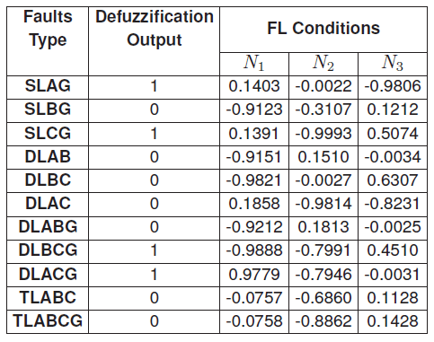
Table 5. CNF fault defuzzication output and FL conditions for the long line at 48 km, R_f= 0.001Ω, fault angle = -2.0892◦ for the different fault types

Table 4 and Table 5 respectively present the long and the short transmission line different fault types, as well as the defuzzification outputs obtained after FL conditions were applied. The obtained defuzzification output for DLAB, DLAC, TLABC and TLABCG are found to be approximately Zero. All the input variables which do not satisfy the conditions of FL were considered “Non-Applicable”fault conditions (N/A). The N/A input variables were used to determine the prediction accuracy error.

Figure 9 presents the sum of area of all faults which occurs at 600 km, R_f = 0.001 Ω and fault angle of -2.08920 without defuzzification for the long line and Figure 10 presents the sum of area of all faults which occurs at 120 km, R_f= 0.001 Ω and fault angle of -2.08920 without defuzzification for the short line.

Figures 9 and 10 are unique for each area where faults may have occurred and could be used to predict either fault classification or fault location. In [2] and [4], the authors demonstrated that the obtained defuzzification output which was tested at 120 km with R_f = 10Ω and a fault angle of 45 degrees shown in Figures 11 and 12 can also be used in order to classify and locate the exact faults that may have occurred in a very high voltage transmission line.

For faults location results, the CNF network structure was considered based on the different parameters obtained by Clarke’s transformation approach.

Fig.9. Sum of faults area for the long line at 600 km, *R_f* = 0.001 Ω, fault angle = -2.0892◦

Fig.10. Sum of faults area for the short line at 48 km, *R_f* = 0.001 Ω, fault angle = -2.0892◦

Fig.11. CNF defuzzification output fault classification for a line that carry 735 kV over 600 km [2].

Fig.12. CNF defuzzification output fault location for a line that carry 735 kV over 600 km [2].

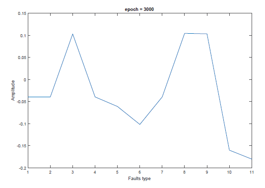
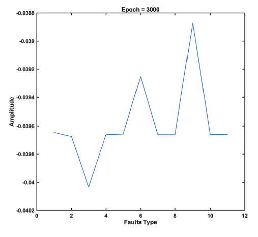
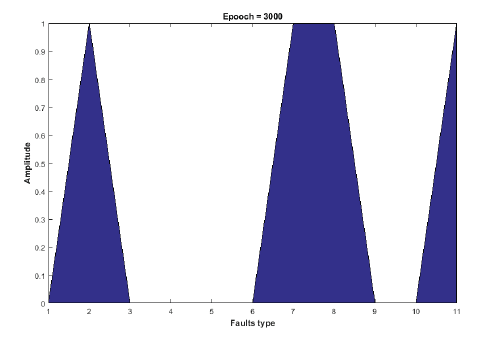
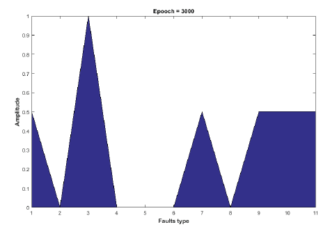
Table 6. Desired and Predicted fault location for the Long Transmission Line with R_f = 0.001Ω, fault angle = -2.0892◦

However, each parameter has been assigned single neuron thus, the structure of the CNF algorithm for the location of the faults was 6-6-6-6-3. The total achieved prediction accuracy for the long line is approximately 99.2309% for fault location and 97.77% for the short line. Table 3 presents various error obtained in respect of a range of data used in simulation.

Table 6 and Table 7 show the long and the short line fault type with its location predicted either at 600 km or at 120 km for the long transmission line and at 120 km and 48 km for the short line. Table 8 and Table 9 illustrate the fault location prediction errors for different locations for long and short transmission lines respectively with fault resistance of 0.001Ω and fault angle of -2.0892 degrees.

Table 7. Desired and Predicted fault location for the short Transmission with R_f = 0.001Ω, fault angle = -2.0892◦

Table 8. Fault location errors for the long transmission line with R_f = 0.001Ω, fault angle = -2.0892◦

Table 9. Fault location errors for the short transmission line with R_f = 0.001Ω, fault angle = -2.0892◦

The fault locations errors were determined using equation 16. Comparing these two tables, it can be seen that at 120 km distance in Table 8, the obtained prediction errors are less than the 120 km distance in Table 9. This could be because of the nature of the utilized dataset.

The worst case scenario is likely to happen at any time if one of the fuzzy rules is not respected. For fault classification according to Table 5, the worst case is SLCG, appeared at 48 km with R_f = 0.001 ohm, fault angle = -2.0892 degree. This problem may occur for some reasons such as, the human error, the error on your data or/and on the algorithms.

In overall, the fault location algorithm for these two cases is more accurate for the long transmission line. However, The study results and findings clearly show that the proposed methodology to evaluate the system error is reliable and can achieve high accuracy which also support the results found in the previous studies published in [2] and [4].

Conclusion

In this article a novelty technique capable of detecting and locating faults in power transmission lines using the state of the art concurrent fuzzy neural network was developed. This technique was applied on two distinct power transmission lines that carry 750 kV over a length of 600 km for the long line and 400 kV over a 120 km length for the short line.

The challenge of applying this technique is to get a sufficient amount of dataset and defining FL rules. Thus, the experiment were carried out using Matlab/Simulink. Post-faults current and voltage were simulated and the obtained values were used as the data set. The proposed fault detection system algorithm for CNF was designed and tested using several faults data sets. Results showed that for both the fault classification and the fault location experiments, the CNF proposed technique achieve high accuracy for both long and short lines. However, the highest prediction accuracy of 97.5% for fault type detection and 99.2309% for fault location from the long line case study was obtained. This can be explained by the fact that the same FL conditions were applied on both systems and these conditions where determined using only the post-faults data from the long line. Thus, the experimental classification results could be improved by acting on the established conditions such as assigning separate rules to each power transmission line.

A comparison was made with other studies which investigate similar cases using CNF technique for fault classification and fault location was introduced. The results and findings of this experiment supports the findings for the other studies that CNF could be reliable and would perform well for the application of fault type classification and location on power transmission lines. It was shown that the defuzzification output can be used to classify various fault types and to locate them.

Finally, it can be concluded that the CNF could be used for fault prediction over three phase power transmission lines. Predicting fault location and fault type with high accuracy could minimize the maintenance cost and time. This will increase the power transmission process efficiency and reliability. CNF technique can also be tested on even longer transmission lines than the 600 km length studied, medium lines and even on multiphase power transmission lines such as six-phase system. Moreover, the effect of including CT could be investigated in future studies in order to determine the influence of using CT on the classification accuracy and the experimental results.

This CNF technique could be applied in various engineering fields following the procedure provided. The choice of parameters or inputs variables depend on the expert and will influence the results obtained.

REFERENCES

[1] Glover, J.D., Sarma, M.S. and Overbye, T., 2012. Power system analysis & design, SI version. Cengage Learning.
[2] Eboule, P.S.P., Pretorius, J.H.C., Mbuli, N. and Leke, C., 2018, October. Fault Detection and Location in Power Transmission Line Using Concurrent Neuro Fuzzy Technique. In 2018 IEEE Electrical Power and Energy Conference (EPEC) (pp. 1-6). IEEE.
[3] Cecati, Carlo and Kaveh Razi, (2012), Fuzzy-logic-based high accurate fault classification of single and double-circuit power transmission lines. In International Symposium on Power Electronics, Electrical Drives, Automation and Motion, pp. 883-889. IEEE.
[4] Eboule, P.S.P., Pretorius, J.H.C. and Mbuli, N., 2018, November. Artificial Neural Network Techniques apply for Fault detecting and Locating in Overhead Power Transmission Line. In 2018 Australasian Universities Power Engineering Conference (AUPEC) (pp. 1-6). IEEE.
[5] Aker, E., Othman, M.L., Veerasamy, V., Aris, I.B., Wahab, N.I.A. and Hizam, H., 2020. Fault Detection and Classification of Shunt Compensated Transmission Line Using Discrete Wavelet Transform and Naive Bayes Classifier. Energies, 13(1), p.243.
[6] Bachmatiuk A, I˙zykowski J. Distance protection performance under inter-circuit faults on double-circuit transmission line. Przeglad Elektrotechniczny. 2013;89(1):7-11.
[7] Dong AH, Geng X, Yang Y, Su Y, Li M. Overhead line fault section positioning system based on wireless sensor network. Przegla˛d Elektrotechniczny. 2013;89(3b):60-1.
[8] Kapoor, G., 2019. Detection and classification of four phase to ground faults in a 138 kV six phase transmission line using Hilbert Huang transform. International Journal of Engineering, Science and Technology, 11(4), pp.10-22.
[9] Kapoor, G., 2019. Protection technique for series capacitor compensated three phase transmission line connected with distributed generation using discrete Walsh-Hadamard transform. International Journal of Engineering, Science and Technology, 11(3), pp.1-10.
[10] Farshad, M., 2019. Detection and classification of internal faults in bipolar HVDC transmission lines based on K-means data description method. International Journal of Electrical Power & Energy Systems, 104, pp.615-625.
[11] Hassani, H., Razavi?Far, R. and Saif, M., 2019, October. Locating Faults in Smart Grids Using Neuro?Fuzzy Networks. In 2019 IEEE International Conference on Systems, Man and Cybernetics (SMC) (pp. 3281-3286). IEEE.
[12] Pouabe Eboule, P.S., Hasan Ali, N., Bhekisipho Twala, (2018) The use of multilayers perceptron to classify and locate power transmission line faults. In Artificial Intelligence and Evolutionary Computations in Engineering Systems, pp.51-58. Springer, Singapor.
[13] Pasupathi Nath R. and Nishanth Balaji V., (2014), Artificial Intelligence in Power Systems. IOSR Journal of Computer Engineering, p.2278-0661.
[14] De Metz-Noblat,B., Dumas, F. and Poulain, C., (2005) Cahier technique n 158 : Calcul des courants de court-circuit, Schneider Electric Collection technique.
[15] Hasan Ali, N., Pouabe Eboule, P.S., Twala B, (2017), The use of machine learning techniques to classify power transmission line fault types and locations. International Conference on Optimization of Electrical and Electronic Equipment (OPTIM) and Intl Aegean Conference on Electrical Machines and Power Electronics (ACEMP), pp. 221-226.
[16] Razi, K., Hagh, M.T. and Ahrabian, G., (2007) High accurate fault classification of power transmission lines using fuzzy logic. In IEEE Power Engineering Conference.
[17] Galyga, A., Prystupa, A. and Zhuk, D., (2016) The clarification method of power losses calculation in wires of transmission lines with climatic factors. In Intelligent Energy and Power Systems, 2nd International Conference. pp: 1-4, IEEE. June 2016.
[18] Rakpenthai, C. and Uatrongjit, S., (2016) Power System State and Transmission Line Conductor Temperature Estimation. IEEE Transactions on Power Systems.
[19] Jiang, J.A., Chuang,C.L., Wang, Y.C., Hung, C.H., Wang, J.Y., Lee, C.H. and Hsiao. Y.T., (2011), A hybrid framework for fault detection, classification, and location Part I: Concept, structure, and methodology. IEEE Transactions on Power Delivery, 26(3), pp.1988-1998.
[20] Sadegheih, A. and Drake, P.R., (2002), Network planning using iterative improvement methods and heuristic techniques. Vol. 15(1), pp.63-74.
[21] Rahimi-Mirazizi, H. and Agha-Shafiyi, M., (2018), Evaluating Technical Requirements to Achieve Maximum Power Point in Photovoltaic Powered Z-Source Inverter. International Journal of Engineering, 31(6), pp.921-931.
[22] Shafiee-Chafi, M.R. and Gholizade-Narm, H., (2014), A novel fuzzy based method for heart rate variability prediction., 27(7), pp.1041-1050, 2014.
[23] Sanjay, C. and Prithvi, C. (2014), Hybrid intelligence systems and artificial neural network (ANN) approach for modeling of surface roughness in drilling, Vol: 1(1), p.943935.
[24] Vieira, J., Dias, F.M. and Mota, A., (2004), Neuro-fuzzy systems: a survey. In 5th WSEAS NNA International Conference.
[25] Yadav, A. and Swetapadma, A., 2015. Enhancing the performance of transmission line directional relaying, fault classification and fault location schemes using fuzzy inference system. IET Generation, Transmission & Distribution, 9(6), pp.580-591.
[26] Popov, M., Rietveld, G., Radojevic, Z. and Terzija, V., (2013), An efficient algorithm for fault location on mixed line-cable transmission corridors. In International Conference on Power Systems Transients (IPST).
[27] Gilany, Mahmoud, E.S., Tag El Din, Abdel Aziz, M.M. and Khalil Ibrahim, D., (2005), An accurate scheme for fault location in combined overhead line with underground power cable. In IEEE Power Engineering Society General Meeting. pp.2521-2527.
[28] Bunnoon, P., (2013), Fault detection approaches to power system: state-of-the-art article reviews for searching a new approach in the future. International Journal of Electrical and Computer Engineering, 3(4), p.553.
[29] Heidari, M., (2017), Fault Detection of Bearings Using a Rule-based Classifier Ensemble and Genetic Algorithm, IJE TRANSACTIONS A: Basics Vol. 30, No. 4, pp 604-609.
[30] Youssef,O.A., (2004),Combined fuzzy-logic wavelet-based fault classification technique for power system relaying, IEEE transactions on power delivery, 19(2), pp.582-589.
[31] Looney, C.G. and Dascalu, S., (2007), A Simple Fuzzy Neural Network. In CAINE pp. 12-16.
[32] Jang, J.S.R., (1991), Fuzzy Modeling Using Generalized Neural Networks and Kalman Filter Algorithm, In AAAI (Vol. 91, pp. 762-767).
[33] Prasad, A., Edwar, J.B., Roy, C.S., Divyansh, G. and Kumar, A., (2015), Classification of Faults in Power Transmission Lines using Fuzzy-Logic Technique. Indian Journal of Science and Technology, 8(30).
[34] Wang, H. and Keerthipala, W.W.L., (1998), Fuzzy-neuro approach to fault classification for transmission line protection. IEEE Transactions on Power Delivery, 13(4), pp.1093-1104.
[35] Gilany,M., El Din, E.T., Aziz, M.A. and Ibrahim, D.K. (2005), An accurate scheme for fault location in combined overhead line with underground power cable. In Power Engineering Society General Meeting, IEEE (pp. 2521-2527). IEEE.
[36] Ray, P., (2014), Fast and accurate fault location by extreme learning machine in a series compensated transmission line. In Power and Energy Systems Conference: Towards Sustainable Energy, 2014 (pp. 1-6). IEEE.
[37] Subramani, C., Jimoh, A.A., Sudheesh, M. and Davidson, I.E. Fault investigation methods on power transmission line: A comparative study. In Power Africa, 2016 IEEE PES (pp.93-97). IEEE.

Source & Publisher Item Identifier: PRZEGLA˛D ELEKTROTECHNICZNY, ISSN 0033-2097, R. 97 NR 1/2021. doi:10.15199/48.2021.01.07

VPN-Based Monitoring Power System Facilities

Published by Petro Baran¹, Yuriy Varetsky¹,², Viktor Kidyba¹, Yaroslava Pryshliak¹, Іgor Sabadash¹, Oleksandr Franchuk³, Lviv Polytechnic National University (1), AGH University of Science and Technology (2), Institute of Microprocessor Control Systems for Power System Objects, Lviv, Ukraine (3),

Abstract. Power system substations are usually controlled from a central control point using various telemechanical systems. At most substations in Ukraine without permanent staff, operational maintenance and control are carried out either by operational field teams or remotely using telemechanical systems. Nowadays, all over the world, as well as in newly built substations in Ukraine, operational and dispatching services apply the principle based on wireless digital technologies. The article presents the results of developing a wireless information network based on ALTRA digital recorders using client-server Virtual Private Network technology.

Streszczenie. Stacje systemu elektroenergetycznego są zwykle sterowane z centralnego punktu sterowania za pomocą różnych systemów telemechanicznych. Obsługa operacyjna i sterowanie większości stacji elektroenergetycznych na Ukrainie, które nie posiadają stałego personelu, realizowane są przez operacyjne zespoły terenowe lub zdalnie za pomocą systemów telemechanicznych. Obecnie na całym świecie, a także w nowo budowanych stacjach na Ukrainie, służby operacyjne i dyspozytorskie stosują zdalne monitorowanie na podstawie bezprzewodowych technologii cyfrowych. W artykule przedstawiono wyniki opracowania bezprzewodowej sieci informacyjnej opartej na rejestratorach cyfrowych ALTRA z wykorzystaniem Virtual Private Network klient-serwer technologii. (Monitorowanie obiektów systemu elektroenergetycznego w oparciu na sieć VPN).

Keywords: ALTRA device, power system, information network, Virtual Private Network.
Słowa kluczowe: Urządzenie ALTRA, system elektroenergetyczny, sieć informacyjna, wirtualna sieć prywatna.

Introduction

A feature of the power system is the location of its facilities (power plants, substations, distribution points) over a large area. They are controlled from dispatching points located at a considerable distance from these objects – up to hundreds of kilometers. The second feature of power systems is the lack of permanent maintenance personnel at these facilities. Such conditions are especially typical for substations and distribution points with rated voltages up to 110 kV. Their operation is controlled remotely through telemechanical systems or with the involvement of operational field teams. The exchange of information between control points and objects of electric power systems is traditionally carried out via telemechanical channels. In the world practice of operating electrical systems, wireless wide-area measurement technologies are increasingly being implemented [1-4]. The use of digital technologies in the automation of power system objects (control, relay protection, signalling and measurement) allows replacing traditional telemechanical communications with modern digital wireless ones [5,6].

One of the tasks of dispatching power system objects is measuring electrical quantities at power plants, substations, distribution points. It includes measuring the operating quantities – voltage on the buses, currents in feeder connections, binary outputs of the electrical installation state sensors, etc. For this purpose, special devices – recorders are installed at the facilities of electric power systems.

Description of ALTRA recorder

The Institute of Microprocessor Control Systems for Power System Objects has developed a series of digital devices ALTRA [7, 8], designed to record operating voltages and currents, as well as binary outputs of state sensors of switching equipment and relay protection under normal operating conditions and in case of emergency events. Digital recorders ALTRA are currently operating at many power facilities in Ukraine. ALTRA devices perform the following functions:

• record the digital oscillograms of the emergency transient electrical quantities;
• control the state of sensor binary outputs of electrical installations;
• save information about emergency events in nonvolatile memory;
• calculate and display on the liquid crystal display the RMS values of all recorded quantities;
• allow viewing the characteristics of emergency events on the liquid crystal display.

The ALTRA device contains analog and binary inputs for monitoring external analog signals (voltages, currents) and binary signals of electrical installations. The device’s connection to the external circuits to monitor the operating condition of the three lines and the substation bus section is shown in Fig. 1.

The operating condition quantities, which are not directly measured, are calculated based on the discretised instantaneous values of the bus phase voltages and the phase currents of the feeders that are directly monitored by the ALTRA device [9]:

• active, reactive and apparent powers in separate phases;
• power factor for individual phases;
• total active, reactive and apparent powers;
• total power factor.

The root-mean-square value of the Y parameter is calculated based on the discrete values measured within the power frequency cycle by the expression:

where T – is the power frequency cycle ( f = 50 Hz); 1 , y_k, y_k₊₁– is the instantaneous values of operating condition quantities (voltages, currents) for k and k+1 sampling points; N – is the number of sampling intervals per cycle; h = T / N – is the sampling step.

Fig.1. ALTRA connection to the external circuits

The calculation of active and reactive powers is carried out by the harmonic sine and cosine components of phase voltages and currents obtained based on Fourier transform as follows:

The sine and cosine components of phase voltages and currents of the i -th harmonic U_si, I_si, U_ci, I_ci are calculated using the next formulas:

A particular information network has been developed for monitoring the operation and testing of ALTRA devices, promptly changing their configuration during operation, reading and analysing digital oscillograms of emergency events stored in the device memory.

When developing an information network, preference is usually given to wired communication. In the absence of physical of information transmission channels, wireless communication with a GSM-based network is used [10, 11]. Until recently, Circuit Switched Data (CSD) technology was used in such wireless information networks.

VPN-based monitoring system

An information network for wireless communication based on Virtual Private Network (VPN) client-server technology has been developed [8] to replace the existing communication system. Secure Shell (SSH) protocol for remote control is used to protect the information in VPN. The OpenSSH library was used to implement this protocol [13, 14].

The use of VPN technology compared to CSD mode has some advantages: higher connection reliability, speed, and online (permanent) connection. Moreover, CSD technology will not be supported by mobile operators in the near future. In addition, the quality of communication in the CSD mode is very low nowadays. Wireless communication based on VPN technology is carried out over a GSM network using GPRS, 3G or 4G standards.

The communication system configuration using VPN technology is shown in Fig. 2. The information network has a two-tier structure. The lower level is formed by digital ALTRA devices installed directly on the object.

Fig.2. Communication system configuration using VPN technology

These devices are connected to the local network via a two-wire communication line type “twisted pair” using the RS 485 interface.

Access to ALTRA devices is organised based on the Hub. The Hub contains a built-in computer, GPS module and GSM modem. It gathers information from all ALTRA devices installed in the facility, its archiving, time synchronisation, and the transfer of information to the higher level of the control hierarchy.

The upper level of the information network consists of an ALTRA-Server and an automated workstation (AWS) of the power site dispatcher, which are connected to the local computer network.

ALTRA-Server consists of a built-in computer and a GSM modem. It collects information from the Hubs installed on the lower level and transmits it to the operator’s AWS for its analysis. ALTRA-Server has a fixed IP address to provide which one can use a SIM-card with a fixed IP address. In terms of controllability, the ALTRA-Server is a passive device. Commands of the Hubs carry out the information transfer to ALTRA-Server, and from the ALTRAServer device to the operator workstation – by the commands of the workstation.

The operator’s AWS is implemented on a personal computer (PC) using special software. It displays the mnemonic diagram of the controlled object (power plant, substation, etc.) on a PC monitor. So, the operator can control ALTRA digital devices, analyse the information registered with them. It is possible to use several operator’s AWS in the control system.

Hub and ALTRA-Server are developed on the platform of the Linux operating system and the operator’s AWS – on the platform of the Windows operating system.

A secure tunnel is created between Hubs and ALTRAServer using SSH protocol based on TCP connection for secure access to information. Asymmetric encryption technology, which involves using a key pair (closed and opened), is used to encrypt and decrypt information. Such an organisation ensures high reliability of data transmission and maximum protection against unauthorised access [10].

For additional protection of the local network, access to the ALTRA Server is carried out from the local network only through the specified ports, and access at the command of ALTRA-Server to the site’s local network is prohibited.

The chart of information flows of the information network on the platform of ALTRA Server is given in Fig. 3. The Hub reads digital oscillogram files from ALTRA devices. They are then transmitted to the ALTRA Server using the SSH protocol. From there, they are read out at regular intervals by the operator’s AWS using the same protocol.

Fig.3. Measurement data flow chart on the ALTRA-Server platform

The possible sampling frequencies of the recording electrical signals in the ALTRA device is set in the device configuration in the range from 1500 Hz to 48000 Hz. From our field experience, the optimal sampling rate of most system transients in terms of aliasing errors, memory using and data transfer rate to the upper level is 3000 Hz or 60 samples for the industrial frequency cycle. However, if there is a need to record high-frequency transients in the power system, one can increase the sampling rate to 48 kHz. Fig. 4 shows an example of the transient behaviour recorded by the ALTRA device under the sampling frequency of 3000 Hz.

Essential functions of ALTRA device control, such as reading/writing configuration, running tests, setting a hub, etc., are executed from the operator’s AWS via VPN using commands that provide authentication.

The developed information network of wireless communication on the platform of VPN client-server technology has been commissioned at many power system objects in Ukraine.

Fig.4. An example of the transient behaviour recorded by the ALTRA device under the sampling frequency of 3000 Hz.

The legal system in Ukraine does not prohibit the use of VPN services, as long as the use of VPN does not violate the rights of third parties and does not pose a threat to national security. VPN service is related to the legislation on personal data protection. Thus, from a legal point of view, the use of VPN data transmission technology in Ukraine is legal. The operation experience of these information networks has approved their high reliability, security and efficiency of data transmission.

Conclusions

The use of ALTRA devices at power facilities provides digital recording operating condition quantities, triggering events of relay protections and circuit breakers, and data transfer to the dispatcher’s automated workstation.

Implementing VPN technology into an information network of the power system objects provides high reliability and security of data transmission and does not require additional technical means.

Digital oscillograms of an emergency event are automatically transferred to the PC monitor of the dispatcher’s automated workstation, along with complete information about the emergency event.

The commissioning of information networks on the platform of VPN technology for the operational maintenance and control of power system facilities creates the basis for developing digital substations.

Acknowledgments: This research was financially supported by the Polish Ministry of Science and Higher Education (grant AGH 16.16.210.476).

REFERENCES

[1] F. Salim, K. M. Nor, D. M. Said, “Experience in online power quality monitoring through VPN,” IEEE 15th International Conference on Harmonics and Quality of Power, pp.482-485, 2012.
[2] D. Karlsson, M. Hemmingsson, S. Lindahl. Wide Area System Monitoring and Control. IEEE Power & Energy Magazine, no.2(5), pp. 68-76, 2004.
[3] K. E. Holbert, G. T. Heydt, And Hui Ni, “Use of satellite technologies for power system measurements, command, and control,” Proceedings of the IEEE, vol. 93, no. 5, pp. 947-955, 2005.
[4] Sun FengJie, QI Qi, Fan JieQing, “Real-time signal time delay analysis of WAMS based on MPLS VPN Technology,” The International Conference on Advanced Power System Automation and Protection, pp. 1089-1093, 2011.
[5] V.I. Vasilchenko, O.G. Hryb, and O.V. Leleka, “Digital substation as a component of the Smart Grid system,” Electrical engineering and electromechanics, № 6, pp. 72-76, 2014.(in ukr.)
[6] V.G Glovatsky, I.V. Ponomarev, “Modern means of relay protection and automation of electric networks,” Energomashvin, 2003, 535 p. (in rus.)
[7] M.V. Bazylevych, R.S. Bozhyk, and I.O. Sabadash, “Microprocessor information-diagnostic system ALTRA for selective identification of grounded phase feeder,” Energy engineering and electrification, Kyiv, № 7, ph. 91 – 95, 2003. (in ukr.)
[8] P.M. Baran, V.P. Kidyba, I.O. Sabadash, and M.V. Bazylevych, “Application of digital devices ALTRA in operational and dispatch control of substations,” Electric networks and systems, № 4-5, pp. 42–45, 2016. (in ukr.)
[9] M.V. Bazylevych, P.М. Baran, V.P. Kidyba, G.M. Lysiak, and I.O. Sabadash, “Physical model of the telemechanical system for operational and dispatch control of substations,” Bulletin of the Lviv Polytechnic National University. Electric Power and Electromechanical Systems, № 870, pp. 3-8, 2017. (in ukr.)
[10] I.V. Gorbaty, А.P. Bondarev, Telecommunication Systems and Networks. Principles of Operation, Technologies and Protocols: textbook. manual, Lviv Polytechnic Publishing House, 2016. (in ukr.)
[11] V.I. Popov, Basics of Cellular Communication of the GSM
Standard, M .: Eco-Trends, 2005. (in rus.)
[12] O. Kolesnikov, B. Hatch. Linux: Creating Virtual Private Networks (VPNs): Trasl. with English, М .: Kudic-Obraz, 2004. (in rus.)
[13] D.J. Barrett, R. Silverman, SSH, The Secure Shell: The Definitive Guide, O’Reilly, 2001.
[14] M. W. Lucas, SSH Mastery: OpenSSH, PuTTY, Tunnels and Keys, Tilted Windmill Press; 2nd ed., 2018.

Authors: assoc. prof. PhD Petro Baran, Lviv Polytechnic National University, E-mail: petro.m.baran@lpnu.ua; assoc. prof. PhD Viktor Kidyba, Lviv Polytechnic National University, E-mail: viktor.p.kidyba@lpnu.ua; assoc. prof. PhD Yaroslava Pryshliak, Lviv Polytechnic National University, E-mail: yaroslava.d.pryshliak@lpnu.ua; assoc. prof. PhD Іgor Sabadash, Lviv Polytechnic National University, E-mail: ihor.o.sabadash@lpnu.ua; Oleksandr Franchuk, Institute of Microprocessor Control Systems for Power System Objects, Lviv, Ukraine, E-mail: olexandr@imskoe.org.ua; prof. DSc Yuriy Varetsky, AGH University of Science and Technology, E-mail: jwarecki@agh.edu.pl

Source & Publisher Item Identifier: PRZEGLĄD ELEKTROTECHNICZNY, ISSN 0033-2097, R. 98 NR 5/2022. doi:10.15199/48.2022.05.03

The Influence of Radiators Construction on Vibroacoustic Measurement of a Power Transformer

Published by Szymon BANASZAK¹, Eugeniusz KORNATOWSKI², Zachodniopomorski Uniwersytet Technologiczny w Szczecinie, Katedra Elektrotechnologii i Diagnostyki (1), Zachodniopomorski Uniwersytet Technologiczny w Szczecinie, Katedra Przetwarzania Sygnałów i Inżynierii Multimedialnej (2)

Abstract. The paper presents an example of transformer tested with complementary tests methods: Frequency Response Analysis and Vibroacoustic Measurement. Methods applied together allow for higher quality of mechanical condition of transformer active part assessment. Presented results show that in some cases application of only one method would be completely misleading. In discussed example a construction of radiators is a source of unexpected vibroacoustic response.

Streszczenie. W artykule przedstawiono przykład transformatora poddanego badaniom komplementarnymi metodami FRA (analiza odpowiedzi częstotliwościowej) i VM (pomiar wibroakustyczny). Zastosowanie obu metod do wspólnej diagnostyki pozwala na zwiększenie trafności oceny stanu mechanicznego części aktywnej transformatora. Przedstawione wyniki wskazują, iż stosowanie tylko jednej z metod może prowadzić do błędów. W omawianym przypadku radiatory są źródłem nieoczekiwanej odpowiedzi wibroakustycznej. (Wpływ konstrukcji radiatorów na pomiar wibroakustyczny transformatora energetycznego).

Słowa kluczowe: FRA, wibroakustyka, transformator, część aktywna, radiator.
Keywords: FRA, vibroacoustic measurement, transformer, active part, radiator.

Introduction

In transformer diagnostics one important issue is assessment of active part’s mechanical condition. The structure of the active part of the transformer must be resistant to various mechanical forces, especially caused by short-circuit currents. Strength of the structure depends on proper connection of all elements, core packages pressure and windings clamping. However, by the time the mechanical structure of the windings and the core deteriorates due to aging of the insulation and cumulative effects of network events or mechanical forces (e.g. transport). The winding can be deformed by the radial and axial forces. Early deformation detection allows for avoiding serious failures and planning of operation and repairs. For the assessment of mechanical condition authors of the paper proposed using two complementary methods: Frequency Response Analysis (FRA) and Vibroacoustic Measurement (VM) [1]. Each of mentioned methods is based on different physical phenomenon, therefore analysis of test results coming from two methods gives much higher quality of assessment. The first assumptions and results were based on laboratory tests and experiment performed on the small unit, which led to first industrial applications. At present the complementary method FRA+VM is introduced into industrial practice in Poland in one of diagnostic companies. However it was found, that in some cases, VM results may not be clear to interpret.

Test object and measurements methodology

The example of such case is transformer TORc 16000/115, 115/16.5 kV, 16 MVA, produced in 2014, and measured one week after installation. It was tested with both methods – FRA and VM – and it was found that they give contrary results. The measurements performed with FRA method are based on the standard introduced in December 2012 [2].

The equipment used for measurements was FRAnalyzer from Austrian company Omicron. The device is equipped with three concentric cables (source, reference and measurement). Screens of the cables were grounded on both sides; in the device and along the bushing with the shortest. The latter is very important for repeatability of test results in high frequencies. The frequency spectrum and number of measurement points were set to allow high resolution of results. The analysis of test results was performed in logarithmic scale by visual comparison of three phases and by application of author’s algorithm. FRA method is capable to detect physical shifts of windings, therefore frequency response results are used mainly for assessment of windings integrity. This method could detect bend winding, which is still clamped (VM will not detect such case), but FRA cannot detect loose winding with lost clamping, when there is no actual physical shift of coils and therefore all capacitances and couplings are unchanged. From this reason the second method was introduced, capable of detecting loose elements due to their mechanical vibrations, which concerns both windings and the core.

The vibroacoustic measurements were done with accelerometric sensor attached to the tank, in the half of its height, while transformer was powered without load. Both transient and steady states were recorded and analyzed. The accelerometric sensor was attached in the middle height of the tank, on the side of the transformer. The sensor and acquisition device was SVAN 958 vibrometer. The methodology of measurement was typical [3, 4], however the analysis of test results was conducted with modified tools.

The conception of VM methodology is based on two main assumptions:

a) In the steady state of transformer operation without load dominant source of vibrations is magnetostriction. The acceleration of magnetostriction vibrations of the core is proportional to the square of power voltage and does not depend from the current value (which is many times smaller than nominal current with load). The analysis of this signal of vibrations allows for assessment of mechanical quality of the core.

b) The analysis of vibrations in the transient state, during the first several dozens of seconds from energizing transformer without load allows for assessment of the technical conditions of the active part. Main sources of vibrations in this case are magnetostriction and windings vibrations caused by interwinding electromagnetic forces. The acceleration of magnetostriction vibrations is, similarly to the point a), proportional to the voltage value, while acceleration of vibrations caused by electrodynamic forces between turns is proportional to the square of the current.

The condition of vibrations in steady state was assessed with author’s method based on the analysis of relative vibrations power in frequency domain a_r(f) [1, 8], defined as follows:

where: P(f,f₁) – vibrations power for frequency range from f to f₁, P(0,f₁) – total vibrations power, from 0 Hz to frequency f₁.

In the VM analysis presented in experimental part of the paper for steady state it was assumed that f₁ = 2.5 kHz. This limit comes from the fact, that above this frequency amplitudes of harmonic frequencies of acceleration signal were negligible small.

The analysis of vibrations in the steady state was performed with two separate tools: in time domain and in frequency-time domain.

The first method is based on the analysis of the envelope of the vibrations signal acceleration [1]. This signal does not fulfil conditions for signal with amplitude modulation (AM) [7], so there cannot be applied typical AM detector, based on Hilbert transform definition. There was used modified AM detector, which is described in [8]. The construction of such modified amplitude detector, similarly to the standard one, is based on the algorithm for calculation of analytical signal module. The basic difference is that in modified detector real and imaginary part of analytical signal is digitally low-pass filtered. This action removes from the amplitude spectrum high frequency components. In addition, input signal is decimated – sampling frequency is lowered N-times if compared to the original sampling frequency. On graphs presented in the paper the envelope of the tank vibrations acceleration signal is described as a_rz(t).

The time-frequency analysis was performed with spectrogram, however the vibroacoustic signal was preliminary applied to the Spectral Subtraction Method algorithm (SSM). SSM was described in Przegląd Elektrotechniczny in 2014 [6]. This method allows for reduction of the magnetostriction influence on the measurement, which results in more detailed conclusions coming from vibroacoustic phenomena caused by current impulse during energizing the transformer without load.

Results of experimental research

FRA results did not show any unexpected differences between phases – see Fig. 1. Visible differences in low frequency range for the middle phase are typical and are a results of different flux distribution in the core (side phases vs middle one) [5]. The second region with visible changes is 10-20 kHz, which is typical for given transformer construction (confirmed by comparison to similar units). There was no possibility to refer these results to previous ones, recorded e.g. before transportation or after installation on-site.

The VM tests in steady state were performed according to the methodology described in [1], there was prepared a graphs presenting normalized spectral acceleration power density (of the signal recorded with accelerometer) of tank vibrations in frequency function a_r(f) . The character of this value changes shows the mechanical integrity of the core. It can be seen (Fig. 2a) that – if compared to perfect case of the core – values of a_r(f) stay high up to 0.4-0.6 kHz, which in theory should be an effect of core problems.

Figures 2b and 2c show the process of vibrations stabilization in transient state, after energizing unloaded transformer. VM diagnostics results shown on Fig. 2b prove that vibrations amplitude stabilization is preceded by many oscillations of tank vibration signal envelope. This phenomenon may be caused by damaged winding clamping system elements or loosening of the core.

Fig.1. FRA results of transformer TORc 16000/115

Fig.2. Changes of normalized spectral power density of tested transformer (a): continuous line – ideal case, dashed line – tested unit, (b) oscillations of the envelope of the transient vibrations signal,(c) spectrogram of transient vibrations signal

The spectrogram presented on Fig. 2c is prepared with SSM. The shape of the spectrogram shows that there are damages in the active part of given transformer. Time of vibrations stabilization exceeds 30 second, which if compared to current impulse (shorter than 0.5 s) is extremely long. In addition, results presented on the spectrogram from Fig. 2c have very rich frequency amplitude spectrum. Vibrations having spectrum up to 6000 Hz last for 15 second, while the amplitude of vibrations at 1 kHz drops to level of -60 dB after 32 seconds.

The latter is completely contrary to FRA results. Its vibroacoustic response gave results, which could be compared to old, aged units. Taking under consideration age of the unit (only one week of operation!) and results of both methods, authors started to analyze what could be the real source of vibrations. It was found that transformer radiators have insufficient mechanical support and stability. They were not connected together with outer metal stabilizers, as it is usually done, and there could be observed vibrations even after mechanical excitation with bare hand. Such construction of radiators was suspected to be the source of unexpected vibrations. An experiment was planned to confirm these assumptions. All radiators were bound together around the transformer with two ratchet cargo tapes – see Fig. 3.

Fig.3. Transformer with radiators bound with cargo tapes

The measurements of vibroacoustic response were repeated and the results were quite different (Fig. 4). With radiators stiffed with the ratchet tape the results of vibroacoustic analysis showed that the transformer’s active part is not in bad condition.

Results of steady state analysis (Fig. 4a) show that mechanical integrity is much better than in previous measurement. The curve a_r(f) drops rapidly at 0.3 kHz (previously at 0.6 kHz). Currently above the frequency 800 Hz the total vibrations power does not exceed 5% of total power. Similar conclusions can be drawn from transient state analysis (Fig. 4b, c). From comparison of Figs. 2b and 4b it can be seen that with transformer construction stiffened (radiators) the oscillations of the signal envelope are much lower in the first seconds after energizing the transformer. There are also significant differences in spectrograms (Figs. 2c and 4c). Before stiffening with cargo tapes the time of transformer’s tank vibrations stabilization was over 30 seconds, while now stabile vibrations in steady state start approx. after 20 seconds. This clearly indicates that the source of previous vibrations were radiators, not the active part of the transformer.

Fig.4. Changes of normalized spectral power density of tested transformer with cargo tapes; (a): continuous line – ideal case, dashed line – tested unit, (b) oscillations of the envelope of the transient vibrations signal,(c) spectrogram of transient vibrations

Summary

The experiment with additional tapes mounted around the radiators showed that vibrations of external constructional elements of the transformer may lead to mistakes in vibroacoustic analysis. However this additional connection cannot be used as a remedy for correct diagnosis. Vibrations of radiators are still the source of VM mistakes, but in smaller scale. This can be observed e.g. in oscillations in transient state (Fig. 4b), which could suggest problems with windings clamping. This example has clearly showed that assessment of the mechanical condition of the active part based only on VM results may be drastically misleading. There is a need for verification with additional method based on different physical phenomenon. In this case the best method is FRA, introduced into complementary FRA+VM analysis. Each of these methods is limited in a different way, so there is a little chance to perform a wrong diagnosis of results coming from two different methods.

REFERENCES

[1] Kornatowski E., Banaszak S., Diagnostics of a Transformer’s Active Part With Complementary FRA and VM Measurements, IEEE Transactions on Power Delivery, 29 (2014), n.3, 1398-1406
[2] IEC 60076-18: Power transformers – Part 18: Measurement of frequency response, International standard
[3] Borucki S., Cichoń A., Subocz J., Kornatowski E., The technical assessment of core and windings in a transient state of power transformer operation, Przegląd Elektrotechniczny, (2010), n.11b, 22-25
[4] Borucki S., Time-frequency analysis of mechanical vibrations of the dry type power transformer core, Acta Physica Polonica A, 120 (2011), n.4, 571-574
[5] Mechanical-Condition Assessment Of Transformer Windings Using Frequency Response Analysis (FRA), Report of CIGRE Working Group A2.26, 2008
[6] Kornatowski E., Application of SSM method in vibroacoustic diagnostics of power transformers, Przegląd Elektrotechniczny, (2014), n.10, 121-124
[7] Zieliński T.P., Cyfrowe przetwarzanie sygnałów. Od teorii do zastosowań, Wydawnictwo Komunikacji i Łączności, Warszawa 2009
[8] Kornatowski E., Cyfrowe przetwarzanie sygnałów wibroakustycznych w bezinwazyjnej diagnostyce transformatorów energetycznych, Wydawnictwo Uczelniane ZUT w Szczecinie, Szczecin 2014

Authors: D.Sc.Eng. Szymon Banaszak, West Pomeranian University of Technology, Department of Electrotechnology and Diagnostics, ul. Sikorskiego 37, 70-313 Szczecin, E-mail: szymon.banaszak@zut.edu.pl,
D.Sc.Eng. Eugeniusz Kornatowski, West Pomeranian University of Technology, Department of Signal Processing and Multimedia Engineering, ul. Sikorskiego 37, 70-313 Szczecin, E-mail: eugeniusz.kornatowski@zut.edu.pl.

Source & Publisher Item Identifier: PRZEGLĄD ELEKTROTECHNICZNY, ISSN 0033-2097, R. 92 NR 8/2016.doi:10.15199/48.2016.08.10

Polish Hydropower Resources and Example of their Utilization

Published by Józef PASKA, Karol PAWLAK, Pola RONKIEWICZ, Paweł TERLIKOWSKI and Jan WOJCIECHOWSKI*Warsaw University of Technology, Institute of Electrical Power Engineering, Poland

Abstract: This paper presents the analysis of Polish rivers’ potential to be employed in the construction of new electricity sources. On the basis of the hydrological data obtained in a number of years, set of parameters for 28 water gauges were assessed. The water gauges chosen were meant to display characteristics representative for the whole country. The analysis was preceded by general information concerning the Polish hydropower sector. Finally, the case study of small hydroelectric power plant (SHP) was presented. The location of the planned power plant is the northern part of Poland, in Suraż near the water gauge on the Narew River.

Streszczenie: W artykule przedstawiono analizę potencjału polskich rzek do wykorzystania w budowie nowych źródeł energii elektrycznej. Na podstawie danych hydrologicznych uzyskanych w ciągu kilku lat oceniono zestaw parametrów dla 28 wodowskazów. Wybrane punkty wodowskazowe miały zobrazować cechy charakterystyczne dla całego kraju. Analiza została poprzedzona ogólnymi informacjami dotyczącymi polskiego sektora energetyki wodnej. Na koniec przedstawiono studium przypadku małej elektrowni wodnej (MEW). Lokalizacja planowanej elektrowni to północna część Polski, w Surażu koło wodowskazu na Narwi. (Zasoby hydroenergetyczne Polski i przykład ich wykorzystania).

Keywords: hydropower industry in Poland, small hydropower plants (SHP), Polish rivers hydropower potential, example of SHP.
Słowa kluczowe: hydroenergetyka w Polsce, małe elektrownie wodne, potencjał energetyczny polskich rzek, przykład MEW.

Introduction

According to the 2030 EU climate and energy framework, the share of renewable energy sources should amount to at least 27% of EU energy consumption [1]. Energy production with the use of hydropower plants is widespread globally, accounting for one fifth of the total global power generation [2].

Poland, a medium-size country in central Europe, has the entire panoply of possibilities to further develop and expand effective sources of electrical energy, which use the power of water flow to produce energy. Due to Poland’s geographical localization, vast majority of watercourses streaming through the country have their river head and river mouth inside the Polish territory. Therefore, the process of development of hydropower sector rests with Polish politicians forming energy policies.

In 2017, hydroelectric power plants in Poland reached a total capacity of 2.376 GW, which is 5.5% of the capacity installed in the Polish energy sector and produced 2767 GWh of electricity, covering 1.7% of the country’s demand [3]. In addition to the larger hydroelectric power plants, there are also over 700 small hydropower plants [4] that are officially classified as renewable energy sources, not hydroelectric power sources, hence their power is not added to hydropower reports. To be called a small hydropower plant in Poland, the source installed capacity must be under 5 MW. In 2017, all small hydropower plants achieved a total capacity of 0.988 GW [5].

The main condition that the river must meet in order to be used in the energy production process is the flow rate higher than the minimum allowable flow, defined as the minimum flow rate to be maintained in a watercourse perpendicular to the structure to maintain biological balance and water consumption downstream [6]. In Poland, this parameter for most rivers is defined and published by the Institute of Meteorology and Water Management (IMGW). If the watercourse chosen for the construction of the energy source is not included in the IMGW publication, the minimum allowable flow should be calculated using the following formula:

where: Q_n – minimum acceptable flow [m³/s], K – correction factor [-], SNQ – average low flow [m³/s]. In such a case, the value of K factor fluctuates between 0.5 and 1.5, and depends on hydrological type of watercourse.

The smallest of small hydropower plants, called micro installations or micro hydropower plants, need flow values even as low as 1 m³/s. Bearing such a possibility in mind, an analysis was carried out to assess the potential of the Polish hydropower resources, putting emphasis on small hydropower plants utilization.

Water gauge data

To perform the analysis, 28 water gauges in Poland were chosen (Table 1 and Figure 1). The selection of these places was based on the following criteria:

‭• the size of rivers in the country, with the attention given to the most significant ones;
‭• places exposed to risk of flood;
‭• water courses representative when it comes to regional or national hydrological conditions.

On the basis of the average monthly flows of the rivers analyzed, average annual value was calculated for each of three flows. Results were presented in Table 2. SWQ means average high flow and SSQ – average of medium flow.

Accurate choice of components for small hydropower plant, particularly water turbine and generator, demands a broad knowledge of not only water flows, but also flow duration curves. These data show how many days a year a certain value is achieved in the analyzed water gauges.

Annual flow-duration data for 28 chosen water gauges were presented in Tab. 3. They refer to lower flows, lasting for over 300 days per year, and should be understood in the following manner: water gauge no. 1, duration of 310 days – during 85% of the year the water flow will be 7.10 m³/s or higher.

Table 1. The list of water gauges selected to carry out the analysis

Fig.1. The map of water gauges selected to carry out the analysis (based on [8])

Data analysis

As it can be seen in Table 2, even the average low flows (SNQ) are in vast majority much higher than the minimal value of 1 m³/s. It means that using water flow as energy source in Poland is highly reasonable, even if only micro installations are considered.

Table 2. Average annual water flows for selected water gauges [7]

Table 3. Annual flow-duration data for selected water gauges

Hydropower plants, especially with storage reservoir, even a small one, are not only sources of electrical energy, but also water flow regulators. On the one hand, they can protect nearby area against water overflow during floods and, on the other hand, retain water to avert drought. On the basis of the average annual water flows, mean percentage differences between chosen water flows (SWQ – SSQ and SSQ – SNQ) were calculated. Taking the data obtained in this way into consideration, one may appoint the location of gauge stations on the basis of the highest flow differences and the location most likely to be hit by floods.

As it can be observed, upland rivers are characterized by significant differences between SWQ, SSQ and SNQ flows – over 200% to nearly 400%. It can mean that average of medium flow could be even four times higher than average low flow. A river bed could not contain as big high-water stage as the mentioned one, what leads to local or regional flooding. Lowland and coastal parts of water courses are marked by lower flows differences, usually below 180%.

In order to assess power that a hydropower plant can generate, mathematical methods should be used. The first step is Bernoulli’s equation (2), presented below:

where: ρ – the density of the fluid (water) [kg/m³], υ– the fluid flow speed at a point on a streamline, [m/s], g – acceleration due to gravity (constant, 9.81 m/s²), h – the elevation of the point above a reference plane (e.g. surface of the Sea) [m], p – fluid pressure at the chosen point [kg/m²].

In such a case, the point of interest is the analysis for those parameters before and behind the plant, which may be rendered as:

A formula (3) on the left demonstrates Bernoulli’s equation for water before the plant (subscript G), and on the right – water behind the plant (subscript D). Importantly, hydropower is in practice a combination of potential energy (E_p), possessed by water due to its altitude, and kinetic energy (E_k), possessed due to its motion. Treating this as a basis, one must take into consideration two more physical laws that, together with Bernoulli’s equation, help to create a formula for hydropower plant power.

where: m – mass is a product of density and volume of an object.

Energy used by the hydropower plant is a difference between a hydropower before and the one behind the plant, which is reflected by the following formula:

Fluid flow speeds before and behind the plant are usually equal [10], so the parts of the equation denoting kinetic energy, may be also reduced. Factoring out g and assuming that the difference between water before and behind the plant is its head H, mentioned above, leads to the following formula:

The result of the formula obtained is energy, therefore equation (6) should be eventually divided by time t, in order to achieve the result in the form of power P. Bearing in mind that flow Q described in the beginning of this paper is a quotient of volume and time, one may formulate the final equation for raw power (capacity) of a hydropower plant P. Substituting constant values ρ) for water 1000 kg/m³) and g a formula ready to be employed during calculations is as follows:

Raw power is a kind of power in case of which losses in turbines, generators and other parts of a plant are not considered, thus its value multiplied by efficiency equals the real power (capacity) of a source. As it is presented in Tab. 3, for the majority of analyzed gauge stations the flow with 310 days flow-duration amounts to over 10 m³/s. Such a water flow value, with a head of 2m and efficiency of the plant of 0.85, is enough to analyze it as an energy source for a plant generating power 167 kW, which could become the power supply for about 15–18 households. There is no reason not to build such sources close to one another, which may lead to generating even a number of megawatts from sources located along a short river section, as short as a few kilometers. While undoubtedly not every river on its whole distance is fit for the purpose of being used for hydropower plant construction, the existing possibilities are worth reflecting upon.

Case study

In order to properly present the potential of hydrological energy, a conceptual design of a small hydroelectric plant (SHP) was prepared on the basis of the analyses carried out. The location of the planned power plant is the northern part of Poland, in Suraż near the water gauge on the Narew River. Fig. 2 shows the location of the water gauge (in the black ellipse), at which a small hydropower plant will be designed. This point, similarly to the map in Fig. 1, is marked with the number 13.

Fig.2. Location of the proposed SHP on the flood hazard map in Poland

This place was chosen because of:

• geographical location, where there are few power plants;
• flood risk on this section of the Narew river, which thanks to the investment will be reduced;
• small average flow and width of the river bed, allowing the use of a hydroelectric power plant on a small watercourse;
• uncertain energy security of the region, caused by the rare occurrence of transmission power infrastructure;
• the availability of land for investment, due to the location outside areas of heavily urbanized or limited environmental restrictions

The area designated for the investment are plots in Suraż with the following numbers: 34.213 and 22.444 (dam and water part of the power plant), 22.28/1 (retention reservoir), 34.420-424 (electric part of the power plant)

In order to select the type and parameters of the water turbine, the data concerning the measuring point in Suraż was analyzed. Tables 4 and 5, and Fig.3 present monthly characteristic flows and average tides of a given duration and with higher ones.

Due to the very high probability of turbine utilization at nominal conditions for at least 70% of days in the year and the data contained in the tables listed above, a turbine with an esophagus of 6-7 m³/s will be used.

The minimization of the flood hazard will be implemented by an artificial retention reservoir with a volume of 630,000 m³, located before the damming up of the power plant in uncultivated land, currently unused. This reservoir, filled during floods of the river, will also be a water storage for a period of low water levels. In addition, it will have a recreational function for the residents of Suraż and the surrounding area, as the area of 10.5 ha allows the use of a reservoir for sailing, leisure, fishing and agro tourism purposes.

Table 4. Monthly characteristic flows for Narew in Suraż [m³/s]

Table 5. Average Q flows of given duration together with higher ones for Narew in Suraż

Fig.3. Chart of flows with higher ones for Narew in Suraż

The damming up, thanks to which it is possible to more efficiently use the energy of flowing water, was designed to achieve a slope of 4.5 m. The height obtained is of rather low value due to the lowland terrain.

On the basis of the above data, the Kaplan turbine – TK30 HAb 1300-290 was matched, which is operating in a horizontal position, and supplying a 362 kW asynchronous generator, all manufactured by HPP. The generator, thanks to the use of permanent magnets, does not require energy consumption from the grid, for magnetizing the rotor. Tab. 6 depicts the dependence of turbine efficiency and power on flow.

In order to optimize the plant’s operation, a frequency converter was selected. A ACS880-77LC-860A / 800A-7 converter was selected for the needs of a small hydropower plant, converter belong to the ACS880 family of devices manufactured by ABB. The inverter is the smallest of fifteen devices in the series and can work with power sources with a total value of up to 800 kW. In the case of the Suraż power plant, the drive will use its capabilities in about 45%. In Table 7 information on electrical parameters of the ACS880-77LC-860A / 800A-7 converter was presented.

Table 6. Dependence of turbine efficiency and power on flow

Table 7. Electrical data of the selected frequency converter

In order to include the designed energy source in the power grid, it is necessary to choose the right transformer. The power generated in the power plant will amount to 300- 370 kW, therefore for its derivation to electric power system (EPS) a medium voltage line of 15 kV will be used and this must also be the voltage of the transformer upper side. The lower side voltage is 525-690 V, which results from the output voltage of the drive. In this case, a transformer with a non-standard 0.6 kV / 15 kV transformation must be made. Assuming a generation at the rated level (362 kW) with an optimal transformer load of 80%, its power must be about 500 kVA. The calculation of this value is shown by the equation (8).

where: S_T– apparent power of the transformer, S_gen – apparent power of the generator, P_gen – active power of the generator, cosφ – generator power factor.

The auxiliaries switchgear of the power plant will operate at a low voltage of 400 V. The transformer will be used for auxiliaries, with a 0.6 kV / 0.4 kV transformation. Accumulator battery will be the emergency power supply for auxiliaries’ switchgear of the power plant. Due to the conceptual stage of the project and the lack of information on the auxiliaries’ switchgear of the power plant, the devices have not been physically selected.

The generation of power in an asynchronous machine requires compensation of the inductive reactive power, therefore a battery of capacitors will also be used. A 29 kvar battery was chosen, which is justified by the calculation (9) and (10).

where: Q_C – capacitor bank power, tgφ_gen– generator’s reactive power factor, tgφ_EPS – EPS reactive power factor of 0.4.

Power output from the power plant, as mentioned above, will take place at 15 kV, from the nearest MV / LV station, located at a maximum of 700 m from the power plant site. 15 kV line will be routed to the energy measurement point of the designed source. The final course of the line has been included in the plan in Fig. 4. The electric scheme of the power plant, with all devices, is shown in Fig. 5.

Fig.4. Land development plan of power plant

Fig.5. Electric scheme of the small hydro power plant

Conclusions

All things considered, the Polish water courses show various hydropower potential. The conditions to build big many-megawatts’ hydropower plants are, admittedly, limited in Poland, but the analysis presented proves that investing in small hydropower plants installations is worth considering. The economic potential of Polish hydropower resources amounts to 24% [4], thus remaining 76%, which equals 6500 GWh per year, can be developed in the future. Due to hydropower plants efficiency even higher than 90% [9], hydropower energy sources may become more and more popular in the future, especially with the Polish law on wind power plant rendered stricter recently.

The potential of small hydropower plants (up to 10 MW) in Eastern Europe is used in approximately 43%, which amounts to 1.923 GW of installed capacity [11]. Due to global economic crisis at the beginning of the decade, rising costs of supporting RES growth, and frequent critics from the Climate Package, government economic incentives have been substantially limited during last years (e.g. Poland).Taking into consideration the above mentioned hydropower potential indicators, one may conclude that the development of small hydropower plants is definitely possible in Poland.

REFERENCES

[1] Proposal for a directive of the European Parliament and of the Council on the promotion of the use of energy from renewable sources (recast), 2016/0382, Brussels 2017
[2] Corley A.-M.: The future of hydropower, IEEE Spectrum, 2010, http://www.ieee.org
[3] Raport roczny z funkcjonowania KSE. Raport za rok 2017, PSE, http://www.pse.pl
[4] Paska J.: Rozproszone źródła energii, OWPW, Warszawa 2017
[5] Potencjał krajowy OZE. Moc zainstalowana. Stan na 31.03.2018, URE, http://www.ure.gov.pl
[6] Minimum acceptable flow measurement, Ultraflux, http://www.ultraflux.net
[7] Fal B. et al.: Przepływy charakterystyczne głównych rzek polskich w latach 1951-1990, IMGW, Warszawa 1997
[8] Mapa zagrożenia powodziowego, ISOK, http://www.mapy.isok.gov.pl/imap/
[9] Jarry-Bolduc D., Côté E.: Hydro energy generation and instrumentation & measurement: Hydropower plant efficiency testing, 2014, http://www.leonardo-energy.pl
[10] Karolewski B., Ligocki P.: Wyznaczanie parametrów małej elektrowni wodnej, Prace Naukowe Instytutu Maszyn, Napędów i Pomiarów Elektrycznych Politechniki Wrocławskiej nr 56, Wroclaw 2004
[11] Liu H., Masera D., Esser L.: World Small Hydropower Development Report 2016 Eastern Europe, UNIDO & ICSHP, 2016, http://www.smallhydroworld.org

Authors: prof. dr hab. inż. Józef Paska, Politechnika Warszawska, Instytut Elektroenergetyki, Zakład Elektrowni i Gospodarki Elektroenergetycznej, ul. Koszykowa 75, 00-662 Warszawa,
E-mail: jozef.paska@ien.pw.edu.pl; dr inż. Karol Pawlak, Politechnika Warszawska, Instytut Elektroenergetyki, Zakład Elektrowni i Gospodarki Elektroenergetycznej, ul. Koszykowa 75, 00-662 Warszawa,
E-mail: karol.pawlak@ien.pw.edu.pl; mgr inż. Paweł Terlikowski, Politechnika Warszawska, Instytut Elektroenergetyki, Zakład Elektrowni i Gospodarki Elektroenergetycznej, ul. Koszykowa 75, 00-662 Warszawa,
E-mail: Pawel.Terlikowski@pw.edu.pl; mgr inż. Pola Ronkiewicz, Politechnika Warszawska. Instytut Elektroenergetyki, Zakład Elektrowni i Gospodarki Elektroenergetycznej ul. Koszykowa 75, 00-662 Warszawa, E-mail: pola.ronkiewicz@ien.pw.edu.pl; mgr inż. Jan Wojciechowski, wojan18@gmail.com

Source & Publisher Item Identifier: PRZEGLĄD ELEKTROTECHNICZNY, ISSN 0033-2097, R. 96 NR 1/2020. doi:10.15199/48.2020.01.01

The Effect of Cable Duct Diameter on the Ampacity of High-Voltage Power Cables

Published by Filip RATKOWSKI¹,², Michał KOŁTUN², Stanislaw CZAPP¹, Gdańsk University of Technology (1), Eltel Networks Energetyka SA (2). ORCID: 1. 0000-0002-4698-9729, 3. 0000-0002-1341-8276

Abstract. The ampacity of power cables depends, among others, on the conditions of heat dissipation from the cable to the environment. Cables are usually laid directly in the ground, but in some sections, they may be placed in ducts, which adversely affects the ampacity of the cable line. The paper presents heat transfer phenomena for cables installed in pipe-type ducts filled with air. The effect of cable duct diameter on this ampacity is discussed. The results of the theoretical analysis have been validated by calculations performed with CYMCAP software. The comparison of the ampacity for air-filled vs. water- or bentonite-filled ducts is also included. The analyses and comparisons have shown that with an appropriate dimension of the duct, the simplest filling (with air) allows to obtain the ampacity not lower than when water or bentonite is used.

Streszczenie. Obciążalność prądowa długotrwała kabli elektroenergetycznych zależy między innymi od warunków oddawania ciepła z kabli do otoczenia. Kable są zwykle układane bezpośrednio w ziemi, ale na pewnych odcinkach stosuje się przepusty kablowe, co niekorzystnie wpływa na obciążalność linii kablowej. W artykule przedstawiono zjawiska wymiany ciepła w rurowych przepustach kablowych wypełnionych powietrzem. Przeanalizowano wypływ średnicy przepustów na tę obciążalność. Wyniki analizy teoretycznej zweryfikowano przy użyciu programu komputerowego CYMCAP. Porównano również obciążalność prądową długotrwałą kabli w przepustach wypełnionych powietrzem z obciążalnością w przypadku wypełnienia przepustów wodą lub bentonitem. Analizy i porównania wykazały, że przy odpowiednich wymiarach przepustu najprostsze wypełnienie (powietrzem) pozwala uzyskać obciążalność kabli w przepustach nie mniejszą niż przy zastosowaniu wody lub bentonitu. (Wpływ średnicy przepustów kablowych na obciążalność prądową długotrwałą kabli elektroenergetycznych wysokiego napięcia).

Keywords: high-voltage power cables, ampacity, cable ducts
Słowa kluczowe: kable wysokich napięć, obciążalność prądowa długotrwała, przepusty kablow

Introduction

In practice, the best possible heat dissipation from cables is needed to ensure their maximum ampacity. The solution for calculating the ampacity of underground power cables proposed by Neher-McGrath [1] has been widely accepted for over 60 years now. Today, the power industry uses IEC 60287-1-1 standard [2], where the Neher-McGrath model contributes a lot.

Generally, the ampacity of a power cable can be calculated from the following dependency [2]:

where (based on [2]) : I_A – ampacity of the power cable, A; Δθ – permissible temperature rise of the conductor above the ambient temperature, K; W_d – dielectric loss per unit length per phase, W/m; T₁ – thermal resistance (per core) between the conductor and sheath, (K.m)/W; T₂ – thermal resistance between the sheath and armour, (K.m)/W; T₃ – thermal resistance of external serving of the cable, (K.m)/W; T₄ – thermal resistance between the cable surface and the surrounding medium (e.g. soil), (K.m)/W; n_c – number of conductors in the cable; R – AC current resistance of the conductor at its maximum operating temperature, Ω/m; λ₁ – ratio of total loss in metallic sheaths to total conductor loss; λ₂ – ratio of total loss in metallic armour to total conductor loss, -.

When the cable line is laid in different ambient conditions, its permissible load depends on the section having the worst ability for heat dissipation. This mainly includes crossings with heat sources such as other power cable lines, heat and steam pipelines, or cables’ sections where laying conditions significantly change (e.g. cables partially laid in pipes/ducts or in free air with possible high insolation) [3–10].

To lay power cables in a significant depth, for long distances, and/or below various obstacles, the method called Horizontal Directional Drilling (HDD) is used (Fig. 1). The HDD is a method of installing an underground pipe/duct with trenchless technology, which involves the use of a directional drilling machine and associated attachments to perform drilling according to the assumed path. When a pipe is installed in the ground, the power cable is pulled inside the pipe. The cables laid in pipes are usually in trefoil formation and a separate pipe should be used for each single-conductor cable.

When the cable is installed in a deep pipe/duct, its ampacity significantly decreases, compared to the directly buried cables, which negatively influences both technical and economic aspects. The key factors affecting the ampacity for this kind of installation are: dissipation of the heat coming from a long distance to the ground surface, thermal resistivity of the pipe/duct filling (bentonite, water, or just air), as well as in the case of bentonite utilization, the effects of possible formation of voids inside the duct resulting from bentonite fluid injection imperfections during the processes of directional drilling [11] and drying-out of the bentonite.

Fig.1. Horizontal Directional Drilling (HDD) machine with ducts pulled over

Fig. 2 presents the results of an experiment examining the bentonite drying-out phenomenon inside the bucket. After taking the original liquid form (during preparation) needed to pour it into a duct, the bentonite changes the characteristics to those of a gel medium – it shrinks and cracks, because of drying-out. According to [12], the thermal resistivity of bentonite is usually below 1.0 (K.m)/W, in both fluid and solid form – and this value (1.0 (K.m)/W) is recommended as the reference for the native soil in various countries while designing cable lines [13, 14]. However, the drying-out process makes that some parts of bentonite filling become behaving as air-filled areas, which negatively influences the originally assumed heat transfer.

Another filling medium in pipes/ducts is water. It is easy to use and has low thermal resistivity (25 times lower than air [8]). The disadvantages of using water as filling medium include the tendency to evaporation and the necessity of refilling when the pipes are unsealed. Moreover, water tends to make a microbiological film on the cable and the internal surface of the pipe, which worsens the heat dissipation.

Fig.2. Effects of bentonite drying-out inside the bucket. Cracks and shrinkage of the bentonite from the bucket wall toward the center progressed within approx. 2 weeks of making the sample

As the CIGRE document reports [15], warmer water tends to collect at higher points of the duct, thus causing a difference of about 10 °C between the temperatures along the length of the pipe/duct. The phenomenon of different temperatures along the water-filled duct was also observed in Distributed Temperature Sensing (DTS) measurements of Stadium – “Powiśle” substations for the 110 kV power cable line in Warsaw, Poland [16]. The maximum temperature difference amounting to around 10 °C along the duct (Fig. 3) reduced the positive effect of water filling in some duct sections.

Fig.3. Maximum and minimum temperatures recorded in DTS measurements for the 110 kV power cable system Stadium – “Powiśle” (along its length) in Warsaw, Poland in 2015 [16]

Taking in mind the aforementioned disadvantages of filling the ducts with water or bentonite, it is reasonable to focus on the optimization of dimensions of cable pipes/ducts filled with air. This type of duct filling is the simplest (compared to bentonite or water), and, as the authors’ further investigation will show, the air-filled duct may give the ampacity not worse than that provided by the water- or bentonite-filled duct.

The further part of the paper presents the investigation of the ampacity of power cables laid in pipe-type ducts. Heat transfer phenomena in such a cable arrangement are analyzed. The effect of pipe diameter on the ampacity of the power cable is presented.

Assumptions for the ampacity analysis

The analysis of the high-voltage power cable ampacity is conducted for the cable line formation depicted in Fig. 4 and ambient parameters colated in Table 1.

Fig.4. The arrangement of the analyzed power cable system; cables in pipe-type ducts: trefoil formation, thermal resistivity of the native soil 1.0 (K.m)/W, ambient temperature (soil) 10 °C

Table 1. Cable type and other parameters assumed in the analysis

If the power cable is laid in a duct, its external thermal resistance T₄, included in (1), consists of three components [17]:

where: T₄’ – thermal resistance of the air space between the cable surface and the duct internal surface, (K.m)/W, T₄” – thermal resistance across the wall of the duct, (K.m)/W; T₄“‘ – external thermal resistance of the duct, (K.m)/W.

The cable arrangement in the air-filled duct is shown in Fig. 5, along with relevant heat transfer components. The heat transfer consists of the following components:

1) convection from the cable surface to the air inside the duct,
2) convection from the air inside the duct to its wall,
3) longitudinal convection due to either forced or natural flow of air along the duct,
4) surface-to-surface radiation from the cable surface to the duct wall.
5) conduction across the duct wall.

Fig.5. Heat transfer in the cable duct (according to [11], with changes)

The thermal resistance T₄” mainly depends on the parameters of the material used to produce the duct and the external/internal diameter ratio. The thermal resistance T₄“‘ mainly depends on the environment around the duct and the area of heat transfer from it. However, from the point of view of the effect of the duct on the cable ampacity, the most interesting term is the thermal resistance T₄’. According to the dependency (3) derived from [17] it can be concluded that for air-filled pipes/ducts, the resultant thermal resistance of the air space between the cable surface and the pipe/duct internal surface does not depend on pipe diameter:

where: D_e– external diameter of the cable, mm; θ_m – mean temperature of the medium filling the space between the cable and duct, °C; U, V, Y – constants depending on the type of installation, given in Table 2.

Table 2. Values of constants U, V and Y used in (3), according to [17]

The above conclusion regarding the thermal resistance T₄’ significantly simplifies the analysis of the ampacity of cables in ducts.

Analysis results

As aforementioned, the ampacity of power cables depends on the intensity of heat dissipation from cables to the surrounding space. For the purpose of the analysis, the total power loss (per unit length) generated in the cable is marked as W_t. Based on Fig. 5, this power loss is dissipated to the environment by convection, conduction and radiation:

where: W_conv,s– natural convection heat transfer rate between the cable external surface and the surrounding medium, per unit length, W/m; W_cond – conductive heat transfer rate in the medium surrounding the cable, per unit length, W/m; W_rad,s-w – thermal radiation heat transfer rate between the cable external surface and the duct (pipe) internal surface, per unit length, W/m.

To evaluate the ampacity of the cable placed in the air-filled duct as a function of duct diameter, an algorithm was created which analytically calculates power loss dissipation from the cable. The components included in (4) can be calculated from the following expressions [4]:

where: h_s – natural convection coefficient at external surface of the cable, W/(K.m²); θs – average temperature of external surface of the cable, °C; θ_w – temperature of internal surface of the pipe, °C; A_s – area effective for convective heat transfer, m², per unit length; ρ – thermal resistivity of the medium inside the pipe, (K.m)/W; A_sr – area of the cable surface effective for heat radiation, m², per unit length; F_s,w – thermal radiation shape factor – its value depends on the geometry of the system; σ_B – Stefan- Boltzmann constant, equal to 5.67.10-8 W/(m²K⁴).

The analyses of thermal resistances T₄, T₄’, T₄“, T₄“‘ in expression (2), heat transfer mechanisms W_t, W_conv,s, W_cond, W_rad,s-w in expressions (4)–(7), and the resulting cable ampacity were performed for conditions given in Fig. 4 and Table 1. With regard to the dimensions of the pipe-type duct, it should be mentioned that the standard dimensional ratio (external pipe diameter to pipe wall thickness ratio) is equal to 11 – it is marked SDR11. The results of the performed analyses, shown in Figs 6–8, have revealed that:

• The thermal resistance T₄’ of the medium (air) inside the duct is constant (Fig. 6), which confirms the conclusion regarding T₄’ from the previous section.
• The thermal resistance T₄” across the wall of the duct (Fig. 6) is constant due to the constant value of the external/internal diameter ratio for the pipe/duct [17].
• The external thermal resistance T₄“‘ (Fig. 6) decreases with the increasing pipe diameter.
• The share of heat dissipation by convection W_conv,s increases with the increasing pipe diameter (Fig. 7), due to more intensive air flow in the pipe/duct.
• For pipes/ducts with relatively small diameter, heat dissipation through conduction plays an important role (W_cond in Fig. 7).

Fig.6. Thermal resistances in the cable duct as functions of pipe/duct external diameter. For description of thermal resistances T₄, T₄′, T₄“, T₄“‘ see expression (2)

Fig.7. Heat transfer rate components W_conv,s, W_cond, W_rad,s-w and total power loss W_tgenerated in the cable duct (per unit length) as functions of pipe/duct external diameter. For description of W_conv,s, W_cond, W_rad,s-w, W_t see expressions (4)–(7)

Fig.8. The ampacity of the power cable system as a function of pipe/duct external diameter (for the cable system and other details see Fig. 4 and Table 1)

• For larger pipe/duct diameters (160 mm or more), the heat dissipated by thermal radiation (W_rad,s-w in Fig. 7) gives around 70% share (W_rad,s-w/W_t) in total heat dissipation.

Consequently, the larger the diameter of the pipe in which the cable is placed, the higher its ampacity (Fig. 8).

When installing a cable in a pipe-type duct, the internal duct diameter is usually at least 1.5 times larger than the external diameter of the cable [18, 19]. For the investigated case, when the cable external diameter is 99.08 mm (see Table 1), the normalized pipe of PE200, SDR11 or larger should be used (the pipe internal diameter is 163.6 mm and it gives the diameter ratio 163.6/99.08 ≥ 1.5). Such a diameter of the pipe/duct results in the ampacity equal to 863.7 A (see Fig. 8). The increase of pipe diameter to 400 mm gives the ampacity equal to 923.2 A (ampacity increase by around 7%).

The above investigation of power cable ampacity has been validated with CYMCAP software [20]. Comparing the results from the analytical approach (Fig. 8) with those obtained from the software-aided calculation (second column in Table 3), it can be concluded that the accuracy is around 1 A.

For a wider comparison of types of duct filling, Table 3 also contains the results of ampacity calculations for ducts filled with water and ducts filled with bentonite. One can observe that, for example, the duct of 160 mm diameter filled with bentonite gives the same ampacity as the duct of 225 mm diameter filled with air. Therefore, in some cases (very long and deep cable ducts), it can be more favourable to use a larger diameter of the air-filled duct (the simplest and cheapest solution) than a smaller diameter duct filled with bentonite or water.

Table 3. The ampacity of the analyzed power cable system in duct for various types of filling calculated with CYMCAP software

Conclusion

The article presents the results of analytical calculations of the ampacity of high-voltage power cables installed in cable ducts. The effect of duct diameter on this ampacity is investigated. The investigation is mainly conducted for cable ducts filled with air, which is the simplest duct arrangement. The results of the analysis have shown that the increase of the diameter of the air-filled duct may give the same ampacity of cables as in the case when the duct of a smaller diameter is filled with water or bentonite. Taking into account problems with effective filling of cable ducts, especially when bentonite is used, for very long and deep ducts the authors recommend the simplest solution: the air-filled duct with properly increased diameter.

REFERENCES

[1] Neher J. H., McGrath M. H., The calculation of the temperature rise and load capability of cable systems, AIEE Transactions, 76 (1957), No. III, 752–772
[2] IEC 60287-1-1:2006 Electric cables – Calculation of the current rating – Part 1-1: Current rating equations (100% load factor) and calculation of losses – General (2006)
[3] Anders G. J., Rating of Electric Power Cables in Unfavorable Thermal Environment, IEEE Press: Piscataway, NJ, USA (2005)
[4] Anders G. J., Rating of Electric Power Cables Ampacity Computations for Transmission, Distribution, and Industrial Applications, McGraw–Hill: New York, NY, USA (1997)
[5] de Leon F., Major factors affecting cable ampacity, IEEE Power Engineering Society General Meeting (2006)
[6] De Mey G., Xynis P., Papagiannopoulos I., Chatziathanasiou V., Exizidis L., Wiecek B., Optimal position of buried power cables, Elektronika ir Elektrotechnika, 20 (2014), 37–40
[7] Liang Y., Zhao J., Du Y., Zhang J., An optimal heat line simulation method to calculate the steady-stage temperature and ampacity of buried cables, Przeglad Elektrotechniczny, (2012), No. 3b, 156–160
[8] Maśnicki R., Heat dissipation from the cable in underground power lines, Przeglad Elektrotechniczny, 97 (2021), No. 5, 74–77
[9] Czapp S., Ratkowski F., Optimization of thermal backfill configurations for desired high-voltage power cables ampacity, Energies, 14 (2021), No. 5, 1452, https://doi.org/10.3390/en14051452
[10] Balzer C., Hinrichsen V., Drefke C., Stegner J., Sass I., Hentschel K., Dietrich J., Improvement of ampacity ratings of Medium Voltage cables in protection pipes by comprehensive consideration and selective improvement of the heat transfer mechanisms within the pipe, Jicable’15 (2015), F2-19, 1–6
[11] Ariaratnam, S., Koo, D. H., & Dyer, M. L., Thermoconductivity effects on electrical installations using horizontal directional drilling. In International Society for Trenchless Technology – 25th No-Dig International Conference and Exhibition, Roma 07: Mediterranean No-Dig (2007), 478–486
[12] HEKOTERM Material technical sheet, Hekobentonity (2017)
[13] IEC 60287-3-1:2017 Electric Cables – Calculation of the Current Rating – Part 3-1: Operating conditions–Site Reference Conditions (2017)
[14] Czapp S., Ratkowski F., Effect of soil moisture on current-carrying capacity of low-voltage power cables, Przeglad Elektrotechniczny, 95 (2019), No. 6, 154–159, doi:10.15199/48.2019.06.29
[15] International Council on Large Electric Systems, CIGRE. A Guide for Rating Calculations of Insulated Cables. Working group B1.35, CIGRE: Paris, France (2015)
[16] Ratkowski F., Analiza obciążalności prądowej długotrwałej linii 110 kV RPZ Powiśle – RPZ Stadion na podstawie danych DTS, XXVI Konferencja Szkoleniowo-Techniczna „Elektroenergetyczne sieci kablowe i napowietrzne KABEL 2019”, Janów Podlaski (2019)
[17] IEC 60287-2-1:2001 Electric Cables–Calculation of the Current Rating–Part 2-1: Thermal Resistance–Calculation of the Thermal Resistance (2001)
[18] Hemant J., Residential, Commercial and Industrial Electrical Systems: Equipment and Selection, Volume 1, McGraw Hill Education (India), (2008)
[19] N SEP-E-004 Elektroenergetyczne i sygnalizacyjne linie kablowe. Projektowanie i budowa (2014)
[20] CYMCAP – software for power cable ampacity rating
[21] International Council on Large Electric Systems, CIGRE. Long Term Performance of Soil and Backfill Systems, Working group B1.41, CIGRE, France (2017)
[22] Jakubowski J., Cichy A., Rakowska A., Wytyczne projektowania linii kablowych 110 kV, PTPIREE (2019)

Authors: mgr inż. Filip Ratkowski, Research & Development Center, Eltel Networks Energetyka SA, Gutkowo 81 D, 11-041 Olsztyn, Poland, E-mail: filip.ratkowski@eltelnetworks.com mgr inż. Michał Kołtun, Research & Development Center, Eltel Networks Energetyka SA, Gutkowo 81 D, 11-041 Olsztyn, Poland, E-mail: michal.koltun@eltelnetworks.com dr hab. inż. Stanisław Czapp, prof. PG, Gdańsk University of Technology, ul. G. Narutowicza 11/12, 80-233 Gdańsk, Poland, E-mail: stanislaw.czapp@pg.edu.pl

Source & Publisher Item Identifier: PRZEGLĄD ELEKTROTECHNICZNY, ISSN 0033-2097, R. 98 NR 3/2022. doi:10.15199/48.2022.03.32

Data-Driven Fault Detection and Diagnosis for Centralised Chilled Water Air Conditioning System

Published by Noor Asyikin SULAIMAN¹, Kai Wern CHUINK¹, Muhammad Noorazlan Shah ZAINUDIN¹, Azdiana Md YUSOP¹, Siti Fatimah SULAIMAN¹, Md Pauzi ABDULLAH², Centre for Telecommunication Research & Innovation (CeTRI), Fakulti Kejuruteraan Elektronik dan Kejuruteraan Komputer (FKEKK), Universiti Teknikal Malaysia Melaka (UTeM), Hang Tuah Jaya, 76100, Durian Tunggal, Melaka, Malaysia (1), Centre of Electrical Energy Systems (CEES), School of Electrical Engineering, Faculty of Engineering, Universiti Teknologi Malaysia (UTM), 81310 Skudai, Johor, Malaysia (2),
ORCID: 1. 0000-0003-3126-7309; 3. 0000-0001-5621-9632; 4. 0000-0002-1864-1952; 5. 0000-0001-8251-8038

Abstract. The air conditioning system is complex and consumes the most energy in the building. Due to its complexity, it is difficult to identify faults in the system immediately. In this project, fault detection and diagnosis system using decision tree classifier model was developed to detect and diagnose faults in a chilled water air conditioning system. The developed model successfully classified normal condition and five common faults for more than 99% accuracy and precision. A graphical user interface of the system was also developed to ease the users.

Streszczenie. System klimatyzacji jest złożony i zużywa najwięcej energii w budynku. Ze względu na swoją złożoność trudno jest od razu zidentyfikować usterki w systemie. W ramach tego projektu opracowano system wykrywania i diagnostyki usterek wykorzystujący model klasyfikatora drzewa decyzyjnego do wykrywania i diagnozowania usterek w systemie klimatyzacji wody lodowej. Opracowany model pomyślnie sklasyfikował stan normalny i pięć typowych usterek, zapewniając ponad 99% dokładności i precyzji. W celu ułatwienia użytkownikom opracowano również graficzny interfejs użytkownika systemu. (Wykrywanie i diagnostyka usterek w oparciu o dane dla scentralizowanego systemu klimatyzacji na wodę lodową)

Keywords: Air Conditioning System; Decision Tree; Fault Detection and Diagnosis.
Słowa kluczowe: diagnostyka, system klimatyzacji.

Introduction

The demand for heating, ventilation and air conditioning (HVAC) systems have increased dramatically in recent years. In non-residential buildings, HVAC systems utilise up to 50% of the total electricity consumption [1][2]. Therefore, their efficiencies have a significant impact on the total energy performance of these buildings [3]. The centralised chilled water air conditioning system includes components such as a chiller, cooling tower and air handling unit (AHU). Furthermore, all components are interconnected, and faults in each component may affect the performance of other components. Therefore, when the system operates in faulty conditions, it increases the energy usage of the building. It also may create thermal comfort problems among occupants and reduce the component’s lifetime [4].

Early detection of faults and diagnosis of their root cause enables the correction of the fault before additional damage to the system [5]. Thus, fault detection and diagnostics (FDD) techniques are often used to monitor building systems and have gained interest among researchers. There are three methods of FDD; modelbased methods, rule-based methods and data-driven methods. Model-based methods, as proposed in Li et al. [6], Trothe et al. [7] and Alexandersen et al. [8], uses physical knowledge to describe the system to achieve analytical redundancy in order to detect and diagnose the cause of faults. Likewise, Beghi et al. [9] proposed the model-based approach to detect and diagnose common faults in chiller systems. However, the drawbacks of the model-based method are that it can be very complex and faults modelling availability is limited [10].

In contrast, rule-based methods use expert knowledge to describe the behaviour of the system. For instance, Lauro et al. [11] proposed a fuzzy approach for FDD in the AHU system. However, this technique may have conflicting rules issues, especially for a complex system that requires more rules [5]. Therefore, some researchers such as Eboule and Hasan [12], Sulaiman et al. [13], Mattera et al. [14], and Deshmukh et al. [15] combined both model-based and rule-based methods to improve the outputs.

Recently more researchers have gone into data-driven methods, where it is a more straightforward approach. It only requires historical data of the system. Li et al. [16], Fan et al. [17], and Luo et al. [18] have successfully implemented data-driven FDD for chiller systems. Meanwhile, Yun et al. [19], Piscitelli et al. [20], Yan et al. [21] and Li et al. [22] proposed this method in the AHU system. As no research combines all faults in the entire system, Sulaiman et al. [23] have proposed data-driven FDD to identify faults in the centralised air conditioning system. The system is inclusive of the chiller, AHU and cooling tower systems. They successfully applied three machine learning classifiers; multilayer perceptron (MLP), support vector machine (SVM), and deep learning. All classifiers can identify all six common faults in the centralised system.

Decision-tree methods are one of the data-driven FDD methods available. It has been used in several FDD areas, such as in photovoltaic systems [24], transmission lines [25] and industrial machinery [25][26]. Furthermore, it is a topdown method where relevant attribute classes are developed before classifying the data [28]. In other words, the decision tree approach is a realistic, reasonable, and effective approach [29]. For instance, Balasubramaniam [30] and Li et al. [31] successfully implemented this method in detecting faults in AHU and variable refrigerant flow (VRF). However, this technique is not widely used in air conditioning systems as other machine learning methods.

Therefore this paper aims to develop a fault detection and diagnosis (FDD) system using the decision tree classifier model. Datasets from lab-scale centralised chilled water system were used to train and test the developed system. The Decision Tree model is then compared with Support Vector Machine (SVM) and K-Nearest-Neighbors (KNN). A user-friendly graphical user interface (GUI) for the system is also developed to ease the users.

This paper is written in four sections. It starts with some basic background in Section 1. Whereas Section 2 explains the details of the project methodology of this paper. It is inclusive of the development of decision tree FDD and GUI of the system using MATLAB. Then, the results are presented and discussed in Section 3. Lastly, a conclusion is drawn in Section 4 to deduce the outcomes of this project.

Methodology

This section explains the overall flow of this project from lab-scaled setup, data classification, data pre-processing, training, and testing the machine learning model and lastly, developing the GUI for the FDD system.

Experiment Setup

A lab-scaled centralised chilled water system as in [13], [23], [32] was used in this project is shown in Fig.1. It is a centralised chilled water system with 2 test rooms. Fourteen sensors consisting of temperature, air flow rate, water flow rate, and current sensors were installed in the prototype. The locations were depicted as in Fig.1. The sensors generated fourteen parameters data for the FDD and were logged every second using two data acquisition cards. Approximately 21000 total data samples were collected from the lab-scaled system for each condition. The conditions simulated are discussed in the following subsection.

Data Classification

The data was classified into six conditions, as shown in Table 1. Type 1 was the normal condition of the system, which is fault-free data. Types 2 to 6 were faults data which are commonly occurred throughout the entire system. They are a combination of soft and abrupt faults. An abrupt fault is a sudden change in system behaviour pattern due to total component breakdown, such as compressor malfunction. Thus, it is easy to detect due to the impact on the system. However, it is costly to repair. In contrast, soft faults such as damper stuck and air ducting leakage do not change the system behaviour immediately but develop through time. The fault is usually small and almost unnoticeable at the beginning. However, the fault is noticeable in the long run and has a significant impact on the system.

Table 1. List of conditions

Features extraction

The input data from sensors were segmented for mean and standard deviation values for every 5 seconds interval. As a result, the sampling data has been reduced to 4200 for each dataset, whereas the parameters have increased to This process generated a total of 604,800 data for all condition types with 25,200 instances and 28 parameters. The data were split into 70% for training and 30% for testing the model.

Simulation Setup

The models of the decision tree, SVM and KNN, were developed using MATLAB software. As for the decision tree model, the maximum split of the tree was set to 20 splits, and the tree induction was based on classification and regression tree (CART). Meanwhile, the SVM kernel function was the linear kernel. Lastly, the number of neighbours in the KNN model was 10, and the distance metric was Euclidean. The setting is summarised in Table 2.

Table 2. Simulation setting

GUI Setup

Two GUIs for decision tree FDD was developed using the MATLAB App Designer tool. Users can choose either of these two GUIs to detect and diagnose the conditions listed in Table 1. It also allowed users to extract the input features before diagnosing the fault. The first GUI allowed users to import an entire raw dataset to detect and diagnose the fault. The dataset can be in either “.xlsx” or “.cvs” format.

Fig.1. The schematic diagram of the system with sensors

The layout of the GUI is shown in Fig.2. Meanwhile, the second GUI allowed users to insert five randomly sample data from the same condition type. The sequence of parameters format was shown on top of the interface. The layout of the second GUI is shown in Fig.3. Both GUIs were developed for the decision tree model.

Results and Analysis

This section explains the classification results for the decision tree, SVM and KNN model. The results are presented in the confusion matrixes, where the models’ accuracy and precision can be identified. It summarises how successful the classification model predicts all classes, indicating the correlation between actual results and predicted results. It also can identify the mistake patterns. Thus more training data or new parameters can be added to improve the models’ classification.

A fundamental concept about the confusion matrix is shown in Table 3. True positive is the number the model correctly predicts the positive class. Similarly, true negative is the number the model correctly predicts the negative class. Meanwhile, false positive is when the model incorrectly predicts the positive class, and false negative is when the model incorrectly predicts the negative class.

Table 3. Confusion matrix

Decision Tree Model

Table 4 and Table 5 show the confusion matrixes for the training and testing dataset of the decision tree model. Both tables show that Type 4, 5, and 6 have achieved 100% accuracy. While Type 1, 2 and 3 have some incorrectly classified data. Likewise, Fig.4 shows the overall performance of the decision tree model. The model can identify all condition types accurately and precisely for more than 99% for both training and testing datasets.

Table 4. The training dataset results

Table 5. The testing dataset results

Fig.4. Overall performance of Decision Tree model.

SVM Model

Fig.5 shows the overall performance of the SVM model. The model recognised all condition types with accuracy and precision of over 99% for both training and testing datasets. The accuracy and precision of the SVM model are slightly lower than the decision tree model.

Table 6 and Table 7 show the confusion matrixes for the training and testing datasets of the model. The results show that almost all types have slightly lower accuracy compared to the decision tree model. However, the misclassification rates were only about 0.06% to 2.5%.

Table 6. The training dataset results

Table 7. The testing dataset results.

KNN Model

Fig.6 shows the KNN classifier model performance. The classifier can distinguish the condition types with accuracy and precision for more than 97%. However, the results were slightly lower than the decision tree and SVM model.

Table 8 and Table 9 show the confusion matrixes of the training and testing datasets of the KNN model. From Table 8, the lowest accuracy achieved was 96.8% for Type 1, similar to Type 1 in Table 9, where it has the lowest accuracy at 95.8%.

Table 8. The training dataset results

Table 9. The testing dataset results

Fault detection and diagnosis system GUI

Fig.7 shows the dataset of Type 2 was tested on the first developed GUI. The GUI successfully classified the input data as Type 2 with an accuracy of 99.90%. Only four instances data were misclassified into normal condition.

Meanwhile, Fig.8 shows the GUI result of five sample data from Type 3, compressor malfunction, tested on the second GUI. The system was successfully classified the sample data as Type 3 data. Neither accuracy nor precision percentages were displayed in the second interface.

Fig.7. The type 2 dataset was tested on the first GUI.

Fig.8. Five sample data from Type 3 was tested on the second GUI.

Discussion

Fig.9 shows the overall performance for the decision tree, SVM and KNN model. The graph clearly shows that all three models successfully classified all types with more than 97% accuracy and precision. The decision tree model has the highest accuracy and precision among all.

Fig.9. Overall performance for all three machine learning classifiers; decision tree, SVM and KNN.

Conclusion

The first part of this project discussed the performance of three machine learning models: decision tree, SVM and KNN for data-driven FDD in a centralised chilled water air conditioning system. All classifiers successfully classified six condition types of one normal condition and five faulty conditions. The faulty conditions were among the common faults in the centralised system. Although all classifier models achieved good performance, the decision tree model is the best among all. The accuracy and precision of the decision tree achieved over 99.9% for both training and testing datasets. The second part discussed the developed GUIs for the FDD system using the trained decision tree model. Both GUIs were able to process and classify the data into their types.

Acknowledgement The authors would like to thank Centre for Research and Innovation Management (CRIM), Universiti Teknikal Malaysia Melaka (UTeM) for sponsoring this work.

REFERENCES

[1] C. G. Mattera, J. Quevedo, T. Escobet, H. R. Shaker, and M. Jradi, “A Method for Fault Detection and Diagnostics in Ventilation Units Using Virtual Sensors,” Sensors (Basel)., vol. 18, no. 11, pp. 1–21, 2018.
[2] J. Kim, J. Cai, and J. E. Braun, “Common Faults and Their Prioritization in Small Commercial Buildings Common Faults and Their Prioritization in Small Commercial Buildings,” Golden, CO: National Renewable Energy Laboratory, 2018.
[3] M. F. Othman, H. Abdullah, N. A. Sulaiman, and M. Y. Hassan, “Performance evaluation of an actual building air-conditioning system,” in IOP Conference Series: Materials Science and Engineering, 2013, vol. 50, no. 1.
[4] A. Beghi, R. Brignoli, L. Cecchinato, G. Menegazzo, M. Rampazzo, and F. Simmini, “Data-driven Fault Detection and Diagnosis for HVAC water chillers,” Control Eng. Pract., vol. 53, pp. 79–91, 2016.
[5] W. Kim and S. Katipamula, “A review of fault detection and diagnostics methods for building systems,” Sci. Technol. Built Environ., vol. 24, no. 1, pp. 3–21, 2018.
[6] Z. Li et al., “An Effective Fault Detection and Diagnosis Approach for Chiller System,” IFAC-PapersOnLine, vol. 52, no. 10, pp. 55–60, 2019.
[7] M. E. S. Trothe, H. R. Shaker, M. Jradi, and K. Arendt, “Fault isolability analysis and optimal sensor placement for fault diagnosis in smart buildings,” Energies, vol. 12, no. 9, 2019.
[8] E. K. Alexandersen, M. R. Skydt, S. S. Engelsgaard, M. Bang, M. Jradi, and H. R. Shaker, “A stair-step probabilistic approach for automatic anomaly detection in building ventilation system operation,” Build. Environ., vol. 157, no. February, pp. 165–171, Jun. 2019.
[9] A. Beghi, L. Cecchinato, F. Peterle, M. Rampazzo, and F. Simmini, “Model-based fault detection and diagnosis for centrifugal chillers,” Conf. Control Fault-Tolerant Syst. SysTol, vol. 2016-Novem, pp. 158–163, 2016.
[10] Y. Li and Z. O’Neill, “A critical review of fault modeling of HVAC systems in buildings,” Build. Simul., vol. 11, no. 5, pp. 953–975, 2018.
[11] F. Lauro et al., “Building fan coil electric consumption analysis with fuzzy approaches for fault detection and diagnosis,” Energy Procedia, vol. 62, no. June, pp. 411–420, 2014.
[12] P. S. Pouabe Eboule and A. N. Hasan, “Accurate fault detection and location in power transmission line using concurrent neuro fuzzy technique,” Prz. Elektrotechniczny, vol. 97, no. 1, pp. 37–45, 2021.
[13] N. A. Sulaiman, M. F. Othman, and H. Abdullah, “Fuzzy logic control and fault detection in centralized chilled water system,” Proc. – 2015 IEEE Symp. Ser. Comput. Intell. SSCI 2015, pp. 8–13, 2015.
[14] C. G. Mattera, M. Jradi, M. R. Skydt, S. S. Engelsgaard, and H. R. Shaker, “Fault detection in ventilation units using dynamic energy performance models,” J. Build. Eng., vol. 32, 2020.
[15] S. Deshmukh, S. Samouhos, L. Glicksman, and L. Norford, “Fault detection in commercial building VAV AHU: A case study of an academic building,” Energy Build., vol. 201, pp. 163–173, 2019.
[16] B. Li, F. Cheng, X. Zhang, C. Cui, and W. Cai, “A Novel Semi-supervised Data-driven Method for Chiller Fault Diagnosis with Unlabeled Data,” Appl. Energy, vol. 285, pp. 1–13, 2021.
[17] Y. Fan, X. Cui, H. Han, and H. Lu, “Chiller fault diagnosis with field sensors using the technology of imbalanced data,” Appl. Therm. Eng., vol. 159, no. June, 2019.
[18] X. J. Luo, K. F. Fong, Y. J. Sun, and M. K. H. Leung, “Development of clustering-based sensor fault detection and diagnosis strategy for chilled water system,” Energy Build., vol.186, pp. 17–36, 2019.
[19] W. S. Yun, W. H. Hong, and H. Seo, “A data-driven fault detection and diagnosis scheme for air handling units in building HVAC systems considering undefined states,” J. Build. Eng., vol. 35, 2021.
[20] M. S. Piscitelli, D. M. Mazzarelli, and A. Capozzoli, “Enhancing operational performance of AHUs through an advanced fault detection and diagnosis process based on temporal association and decision rules,” Energy Build., vol. 226, 2020.
[21] K. Yan, J. Huang, W. Shen, and Z. Ji, “Unsupervised learning for fault detection and diagnosis of air handling units,” Energy Build., vol. 210, p. 109689, 2020.
[22] J. Li, Y. Guo, J. Wall, and S. West, “Support vector machine based fault detection and diagnosis for HVAC systems,” Int. J. Intell. Syst. Technol. Appl., vol. 18, no. 1–2, pp. 204–222, 2019.
[23] N. A. Sulaiman, P. Abdullah, H. Abdullah, M. N. S. Zainuddin, and A. Md Yusop, “Fault detection for air conditioning system using machine learning,” IAES Int. J. Artif. Intell., vol. 9, no. 1, pp. 109–116, 2020.
[24] R. Benkercha and S. Moulahoum, “Fault detection and diagnosis based on C4.5 decision tree algorithm for grid connected PV system,” Sol. Energy, vol. 173, no. July, pp. 610–634, 2018.
[25] S. H. . Asman, N. F. . Ab Aziz, U. A. . Ungku Amirulddin, and M. Z. A. Ab Kadir, “Decision Tree Method for Fault Causes Classification Based on RMS-DWT Analysis in 275 kV Transmission Lines Network,” Appl. Sci., vol. 11, no. 4031, 2021.
[26] C. K. Madhusudana, H. Kumar, and S. Narendranath, “Fault Diagnosis of Face Milling Tool using Decision Tree and Sound Signal,” Mater. Today Proc., vol. 5, no. 5, pp. 12035–12044, 2018.
[27] M. Golmoradi, E. Ebrahimi, and M. Javidan, “Fault diagnosis of compressor based on decision tree and fuzzy inference system,” Vibroengineering Procedia, vol. 12, pp. 54–60, 2017.
[28] M. S. Mirnaghi and F. Haghighat, “Fault detection and diagnosis of large-scale HVAC systems in buildings using data driven methods: A comprehensive review,” Energy Build., vol.229, p. 110492, 2020.
[29] A. Contreras-Valdes, J. P. Amezquita-Sanchez, D. Granados-Lieberman, and M. Valtierra-Rodriguez, “Predictive Data Mining Techniques for Fault Diagnosis of Electric Equipment: A Review,” Appl. Sci., vol. 10, no. 950, 2020.
[30] V. Balasubramaniam, “Fault Detection and Diagnosis in Air Handling Units with a Novel Integrated Decision Tree Algorithm,” J. Trends Comput. Sci. Smart Technol., vol. 3, no.1, pp. 49–58, 2021.
[31] G. Li et al., “An improved decision tree-based fault diagnosis method for practical variable refrigerant flow system using virtual sensor-based fault indicators,” Appl. Therm. Eng., vol.129, pp. 1292–1303, 2018.
[32] N. A. Sulaiman, M. F. Othman, and H. Abdullah, “Fuzzy logic control of centralized chilled water system,” J. Teknol., vol. 72, no. 2, pp. 57–62, 2015.

Authors: Noor Asyikin Sulaiman, Ph.D., Universiti Teknikal Malaysia Melaka, Malaysia, E-mail: noor_asyikin@utem.edu.my; Kai Wern Chuink, B. Eng., Universiti Teknikal Malaysia Melaka, Malaysia, E-mail: wernchuink@gmail.com; Muhammad Noorazlan Shah Zainudin, Ph.D., Universiti Teknikal Malaysia Melaka, Malaysia, E-mail: noorazlan@utem.edu.my; Azdiana Md Yusop, Ph.D., Universiti Teknikal Malaysia Melaka, Malaysia, E-mail: azdiana@utem.edu.my; Siti Fatimah Sulaiman, Ph.D., Universiti Teknikal Malaysia Melaka, Malaysia, E-mail: sitifatimahsulaiman@utem.edu.my.

Source & Publisher Item Identifier: PRZEGLĄD ELEKTROTECHNICZNY, ISSN 0033-2097, R. 98 NR 1/2022. doi:10.15199/48.2022.01.47

Impact of Harmonic Current on Energy Meter Calibration

Published by Shannon Edwards, Dave Bobick, and Steven Weinzierl, Radian Research, Inc.
Speaker: Steven Weinzierl, Radian Research, Inc., 3852 Fortune Drive, Lafayette, IN, 47905,
USA, Tel: (765) 449-5548, Email: stevew@radianresearch.com

Abstract: This paper compares and contrasts different methods to quantify VAR for single and polyphase energy meters. The results for the different methods will be compared in the presence of different realistic harmonic content scenarios, with sometimes a 30x difference seen in results between the methods. By understanding the differences between VAR methodologies in the presence of harmonics, we can take the next steps towards metrology consensus and standardization on how to measure and calculate them.

1. Introduction

As countries update their energy policy and infrastructure and increase investment in smart grid technologies, there is greater awareness of power and energy measurements. With that comes greater awareness of the increasing gap between consumed real power (watts) and generated apparent power (VA). Furthermore, as electronic devices become more sophisticated with increased semiconductor content, there is a rapid proliferation of highly non-resistive and nonlinear loads. In fact, many of these new non-resistive and non-linear devices are energy conserving devices such as dimmers, energy-efficient motors in new appliances, and compact fluorescent lights that are being deployed as part of the new energy policies.

Historically, reactive power (VAR) has been used to quantify the gap between consumed real power and generated apparent power of an AC electric power system [1]. Reactive power comes from 2 main sources:

1. Phase angle difference between the voltage and current sine waves, primarily due to non-resistive behavior such as device inductance or capacitance.

2. Waveform distortion from non-linear behavior, primarily due to harmonic content.

VAR is easy to determine in the first case of phase angle (non-resistive) contribution via a scaling factor of sin( ); therefore there is consensus among metrologists and measurement experts on how to quantify it.

However, VAR in the second case due to harmonic currents from non-linear loads is more complicated. Combined with the fact that reactive power in general does not transfer energy, there is a lack consensus amongst metrologists on how to measure and calculate VAR in the presence of harmonic content.

Ironically, the issue is further compounded by the observation that compared to older electromechanical meters, newer solid state meters have much smaller measurement error of active energy (watts) when supplied with active harmonic energy [2]. However, the solid state meters have shown widespread variation in VAR results, hence a call for “for an urgent international agreement” [2]. Because the utilities that produce energy need to build expensive base or peak generation plants based on VA and are beginning to charge consumers based on the VAR component, it is an important issue of fair commerce for a consensus to be achieved amongst metrologists.

This paper will:

• Compile and review the most common VAR calculations. 9 different ones are identified and discussed.

• Propose 6 representative waveforms (theoretical and actual recorded) with differing levels of harmonics in them to compare the results of the 9 different VAR calculations.

• Contributions from harmonics out to the 100^th order are included.

• Compare the results of the 9 different VAR calculations across the 6 different representative waveforms.

• Make suggestions for next steps on how to proceed.

2. Compilation and review of best-known VAR calculations

Because there is no standardized nomenclature, the names for the methods were created by the authors and are now being used within the ANSI C12.24 committee.

The 9 identified VAR calculations are classified into 3 broad types:

Pure fundamental calculation appropriate for a pure sinusoidal which by definition includes the effects of only the first harmonic and discards contributions from higher harmonic orders.

Phase shift calculations. This category has 5 variants within it:

• Integral Phase Shift Method Fixed Frequency
• Integral Phase Shift Method Exact Frequency
• Differential Phase Shift Method
• Quarter Cycle Delay Method
• Cross Connected Phase Shift Method

Vector calculations. This category has 4 variants within it:

• Vector Method using VA RMS
• Vector Method using VA Average Responding
• Vector Method using VA RMS & Fundamental Waveforms

A glossary of symbols used in the formulae is given at the end of the paper.

2.1. Fundamental calculation

VARs for each element are calculated by multiplying the fundamental of the voltage times the fundamental of the current times the sine of the phase angle between them:

VAR_i = || Ṽ_i || ⋅ || Ĩ_i || sin(θ_i)

Where the fundamental RMS Voltage and Current are calculated:

2.2. Phase shift VAR calculations

The genesis behind this calculation type is primarily historical: Early analog electromechanical meters could only measure active (real) watthours. By introducing a known reactive element (typically capacitor and resistor network) into the circuit to create a known 90° phase shift on the voltage axis, the watt-hour measurements of the meter could in essence be “tricked” into measuring the reactive component. The added reactive element made the reactive portion of the power active so the meter could measure it, and made the active part reactive to be invisible to the meter.

Once two sides (watts and VARs) of the power triangle are known, the third (VA) can be easily calculated from the power triangle as shown in Fig. 1 [3]:

While the phase shift method was a resourceful way to make the best use of available technology at the time, this method has shortcomings because the selection of the C and R values are frequency specific: Although the phase shift was correct, it would cause amplitude distortion as frequency changed. The proliferation of the phase-shift techniques was the result of future more sophisticated iterations of it to minimize its shortcomings.

Within the phase shift methods, there are integral (integration) methods and differential (differentiation) methods. The concept is based on:

I.e., integrating the voltage axis gives a 90° phase shift. Differentiation works in a similar manner. However:

• Integration attenuates the amplitude of the harmonics
• Differentiation amplifies the amplitude of the harmonics
• With both, the amplitude “distortion” is proportional to the frequency.

So while the phase shift was achieved, it was at the expense of amplitude distortion. These methods then renormalize the amplitude of the integrated (phase-shifted) voltage to create a voltage whose fundamental voltage would be identical in amplitude to the fundamental component of the voltage axis. Originally the frequency could not be measured in real time so a fixed value (60Hz or 50Hz as appropriate) was assumed; later the frequency was measured and used in the calculation or the equivalent R and C values were assigned adaptively in real time.

The equation for the “Integral Phase Shift Method Exact Frequency” method is:

Substituting (2 ×60) or (2 ×50) as appropriate for gives the formula for “Integral Phase Shift Method Fixed Frequency”.

The equation for “Differential Phase Shift Method” is analogously:

The “Quarter Cycle Delay Method” could be digitally implemented with charge-coupled devices to achieve the phase shifting. Its advantage over the earlier integral/differential phase shift methods is that it doesn’t impact the amplitude. Compared to the integration method, it appeared to periodically flip the sign of a given harmonic’s contribution, and so more often than not will make the VAR calculation be more negative. Its equation is:

Finally, the “Cross Connected Phase Shift Method” is based on creating a voltage that is 90° delayed from the voltage axis and adjusting the amplitude to match the amplitude of the voltage axis input. The 90° delay is created by subtracting the voltage phase that is 240° behind from the voltage phase that is 120° behind. The amplitude is then adjusted by dividing by √3. This phase shift and amplitude adjustment assumes that the voltages are balanced and spaced 120° apart. VARs for each element are calculated by multiplying the 90°-delayed amplitude-adjusted voltage times the current and integrating over the fundamental period:

Where the 90° delayed and amplitude corrected voltages are:

This method has been used extensively in 3-phase electromechanical meters. Its biggest shortcomings are:

• The assumption of balanced voltages across the phases. This is rarely true, giving the wrong amplitude value in the calculation.
• The assumption that the voltage phases are exactly 120° apart (rarely true).

2.3. Vector VAR calculations

These methods are all based on measuring VA and Watts, and calculating VAR for each phase from the power triangle (Fig. 1):

where:

“VAR, Vector Method using VA RMS” uses the fundamental and all harmonics in the calculation:

and then substituting into Eq. 1 and Eq. 2.

“VAR, Vector Method using VA Average Responding” works similarly in concept to the Simpson meter with a D’Arsonval meter movement [4]. It’s worth a mention for historical reasons:

One artifact is that the calculated average responding VA can be less than the watts value, contradicting the power triangle shown in Fig. 1. This is because, for example, a voltage signal which is 0 for some time – as in the case of a dimmer – ends up with a low average value. Hence why the RMS method is better.

“VAR, Signed Vector Method using VA RMS, & Fundamental Waveforms” for polyphase meters attempts to prevent cancelling of signs of different harmonics by getting the sign correct with a multiplying factor of

The rest of the equations are the same as for “VAR, Vector Method using VA RMS”. One practical and obvious difficulty with this method is when =0 and the signing factor blows up. L’Hôpital’s rule [5] must be invoked in real-time to determine which infinite value is smaller.

3. Waveforms

The six representative waveforms used to compare the results of the calculations consist of three theoretical ones and three actual ones recorded in the field. Their names and short descriptions are given here, with pictures of them in the following subsections:

Theoretical:

• Sine wave voltage, Sine wave current -60° lag. Current is lagging voltage, simulating an inductor present in the load. This waveform is used as a reality check – all VARs calculations should be scaled by sin(60°), or 0.866.

• Sine wave voltage, Phase dimming 90° conduction angle. This represents an energy-conscious consumer using a light dimmer at ½ power.

• Narrow Current Pulse. With the proliferation of switching and Pulse Width Modulated (PWM) power supplies [6], this type of waveform might be reflected back from the load to the line.

Actual ones: The National Research Council Canada (NRC) recorded actual waveforms (WF) at a variety of sites in the field; labeled them to anonymize them; archived them; and made them available upon request. While the waveforms may look unbelievable, they are indeed real. Using a digital frequency transformer, we parameterized them into harmonics components out to 100^th order to run them through various closed-form VARs calculations given in Section 2.

• NRC WF23. Actual waveform recorded in the field. Its V and I waveforms are fairly symmetric, with the V waveform having smaller high frequency spikes and I waveform have larger amplitude, lower frequency harmonics.

• NRC WF139140. Actual waveform recorded in the field. Its V waveform is asymmetric, indicating the presence of more even harmonics.

• NRC WF13621363. Actual waveform recorded in the field. Its V waveform is mostly symmetric but has significant spikes and sags. The I waveform is nearly square, indicating many high order harmonics.

To better enable comparisons, all waveforms have been normalized to 1Vrms and 1Arms, i.e., 1VArms.

3.1. Sine wave voltage, Sine wave current -60° Lag

3.2. Sine wave voltage, Phase dimming 90° conduction angle

4. Results and discussion

A graphical summary of the results comparing the different VARs calculations for the different waveforms is given below:

Observations on the results for each of the waveforms are as follows:

Sine wave voltage, Sine wave current -60° lag. As expected and hoped, all VARs methods return the same value of 0.866, so this reality check is passed.
Sine wave voltage, Phase dimming 90° conduction angle.

• All integral phase shift methods gave the same value of 0.45088 because the voltage waveform used was a pure sine wave (no harmonics), i.e., || Ṽ_i ||= 0 in VAR_i = || Ṽ_i || ⋅ || Ĩ_i || sin(θ_i) for i 1.

• The vector methods gave noticeably higher values versus the phase-shift methods because the phase-shift methods miss the contributions of the harmonics.
• All the vector RMS methods gave identical values of 0.70539. However the vector average responding method was the clear outlier with a much lower value of 0.10101 because the voltage signal is 0 for an appreciable time, causing a lower average value.

Narrow Current Pulse. Similar comparison as the previous case of phase dimming:

• All integral phase shift methods gave the same value, but it’s 0 – they totally missed the energy. This is because the voltage waveform used was a pure sine wave (no harmonics), i.e., || Ṽ_i || = 0 for i 1.
• The vector methods gave noticeably higher values versus the integral methods – the integral methods were missing energy contributions from higher harmonics.
• All the vector RMS methods gave identical methods of 0.76571. The vector average responding method was again the clear outlier of the group with a much smaller value because the voltage signal is 0 for an appreciable time. In fact, its VAR value was imaginary because erroneously VA < Watt in the radical VAR = √VA² – Watt².

NRC WF23. The RMS vector methods show highest magnitude because they detect the higher harmonics on both the V and I axes. The differential phase shift method is noticeably lower, most likely because harmonics with negative signs got amplified by the differential phase-shift method and erroneously over-subtracted from the overall total. The vector average responding is lower because the I waveform is near zero for an appreciable time.

NRC WF139140. Here is a case with 30x differences between results. The phase-shift methods are erroneously lower because a pure voltage sine wave was assumed and they’re missing the contributions from the higher even harmonics. Again the differential phase-shift method is lower as it is likely amplifying a negative harmonic and over-subtracting its contribution.

NRC WF13621363. Finally, a case where there is disagreement between the vector VA RMS methods. VA RMS is by definition using all positive quantities, so in this case the “VAR, Signed Vector Method using VA RMS, & Fundamental Waveforms” (last green bar) accounts for contributions from negative harmonics and could be more correct.

5. Conclusions

Significant differences are seen in VAR results on a variety of waveforms. Differences are seen in both sign and order of magnitude, and the agreement gets worse as the harmonic content increases. Due to the proliferation of already-installed electric meters with the different VARs methods, suggesting or mandating a single standard method and then retrofitting the field is impractical. The best course of action is for manufacturers, utilities, and consumers to be aware of the differences and act accordingly.

The core issue is equity in billing in the presence of large harmonic content in both the voltage and current waveforms in the power grid. The power triangle (Eq. 1) only works for sinusoidal waveforms and so is no longer valid. Measuring real consumed power (watts) and reactive power (VARs) separately is in a sense a historical crutch which started out because the original meters could only measure real power.

The technology now exists to measure meter VA and VA-h at the point of use. While there still needs to be consensus among metrologists on VA measurements, that it much more likely to happen than achieving consensus on VAR measurements. Because VA is more directly related to actual cost of generation and more likely to achieve consensus on its measurement, it might make sense to start with VA and address VARs later.

6. Acknowledgements The authors gratefully acknowledge the excellent inputs from, and discussions with, the members of the ANSI C12.24 committee.

7. References

1. http://en.wikipedia.org/wiki/AC_power.
2. The Registration of Harmonic Power by Analog and Digital Power Meters, Johan Driesen, Thierry Van Craenenbroeck, and Daniel Van Dommelen, IEEE Transactions on Instrumentation and Measurement, vol. 47, no. 1, Feb. 1998, pp. 195-198.
3. Handbook for Electricity Metering, 10th edition, Edison Electric Institute, pp. 31-21, 2002.
4. http://en.wikipedia.org/wiki/Galvanometer.
5. http://en.wikipedia.org/wiki/L%27H%C3%B4pital%27s_rule.
6. http://en.wikipedia.org/wiki/Pulse-width_modulation.

8. Glossary
Index “i” represents the i^th phase in the poly-phase network. i=1 single-phase, maximum i is 3 for three-phase.
Ṽ_i = Potential component fundamental (1st harmonic order)
Ĩ_i = Current component fundamental (1st harmonic order)
Ṽ_(h)i = Potential component for harmonic order (h)
Ĩ_(h)i = Current component for harmonic order (h)
_(h)i = Phase angle of the potential for harmonic order (h)
_(h)i = Phase angle of the current for harmonic order (h)
V_i= Generalized potential waveform (fundamental and all harmonics)
I_i= Generalized current waveform (fundamental and all harmonics)
i = Phase angle between the fundamental potential and current, (1)iminus (1)i
t = VAR-hour and VA-hour integration interval measured in seconds
T = Fundamental period
k = Number of fundamental periods
= Fundamental angular frequency = 2 f₀, where f₀ is the fundamental frequency
= Start time of integration
|| || = Generally represents the norm of the wave function: 1-norm (Average) or 2-norm RMS.
|X | = Absolute value of X
bV_i= Blondel Theorem transformed Voltages

bV₁ = V₁ −V₂ ,bV₂ = 0 , bV₃ =V₃ −V₂

Source: 2010 NCSL International Workshop and Symposium

Comparing Harmonics Mitigation Techniques

Published by Jonas Persson Comsys AB Fältspatvägen 4, SE-224 78 Lund, Sweden. jonas.persson@comsy, Comparing Harmonics Mitigation Techniques – Revision 3 – 2014-04-08

Abstract— the document at hand compares harmonic mitigation techniques in a range of applications and settings. Theoretical and practical comparisons are made between active and passive series and shunt filters. The overall context is to reduce harmonic loading in a drive system. Advantages and disadvantages of parallel and series approaches is discussed, as well as advantages and disadvantages of active and passive solutions. Practical results are discussed in a number of case studies.

I. BACKGROUND

The reader should be aware of the following concepts: harmonics, notching, voltage distortion, current distortion, and voltage unbalance.

Harmonics in power systems are predominantly caused by various semiconductor-based loads. Most common loads are drive systems (typically transistor based variable frequency drives and occasionally also line commutated DC drive systems).

Harmonics are simply multiples of the fundamental frequency. Hence, the 5th harmonic in a 50 Hz system is the 250 Hz frequency component.

We will now consider a 3-phase rectifier. In the simplified case where the output of the rectifier is a constant DC-current the harmonic orders visible on the AC line can be written as

ℎ=𝑝∗𝑘 ±1, where k=1,2,3…

The amplitude of the harmonics will depend on a number of factors. The grid strength (or stiffness) will interact with the semiconductor load, as well as the equivalent series line impedance, if present. In general, a stronger grid gives higher amplitudes on the current harmonics, but lower amplitudes on the voltage harmonics, all else being equal.

In practical systems and applications, a discussion on reasonable goals for harmonic distortion are needed; for a treatment of this, please see [1].

II. HARMONIC ISSUES

There are a number of reasons to limit the amount of harmonics in a system. The following is a non-exhaustive list of symptoms that may be caused by harmonics;

• Notching
• Motor vibration
• Bearing current
• Overheating
• Nuisance tripping
• Generator tripping/malfunction
• Production stops
• Electrical fires
• Electrical component failure

There is no point in reducing harmonic levels for its own sake; harmonics do not automatically mean problems like the ones mentioned above. This paper will not go into depth on the issues caused by harmonics, but will focus on the various ways of mitigating harmonics, along with both the advantages and disadvantages of those methods.

III. OVERVIEW OF SOLUTIONS

For the remainder of the discussion, compensation solutions will be divided into four broad classes, with two defining factors; (1) whether the solution is active or passive, and (2) whether the solution is used in shunt or in series with the load or device to be compensated. Using this classification, four classes are obtained, with several practical examples in each class;

Table 1. Compensation solutions

Some of the solutions mentioned in the table above are not ideally suited or intended for harmonic mitigation, they are mentioned for the sake of completeness.

The following types of compensation are mentioned for sake of completeness and will not be discussed further. A Thyristor Controlled Reactor (TCR), is a parallel device where thyristors are used with angle firing control to effectively vary the inductance value of a large reactor. TCRs are frequently used in Static VAR Compensator (SVC) solutions to obtain dynamic reactive power control, most often on medium voltage. A Dynamic Voltage Restorer (DVR) can be used to mitigate sags and dips and can in turn be implemented in several ways. A Static Synchronous Compensator (STATCOM) is a power electronics based Voltage Source Converter that is used as a more modern version of an SVC. In essence, a STATCOM is a parallel active filter.

IV. PASSIVE SOLUTIONS – SERIES

The following section describes and compares passive series mitigation solutions.

Line Reactor

A line reactor is a 3-phase series choke placed in front of the rectifier on the line side of a drive. The line reactor will cause a voltage drop as seen from the rectifier; due to being inductive, the series impedance and hence voltage drop is larger the higher the frequency. Typical inductance values are 2-5%. Lower values than 2% have a very limited impact on the harmonics.

Advantages:

• Low cost
• Significantly reduces current distortion
• Adds protection to the rectifier

Disadvantages:

• Impractical in large drives
• Will not meet harmonic regulation levels on its own
• Need to handle full current of load, not only compensation current
• Drops voltage as seen by the drive rectifier

Series Harmonic Filter

The series harmonic filter is designed to significantly reduce harmonics. In a sense it is a series choke with a few added components tuned to trap more of the harmonics. A typical series harmonics filter can be seen in the figure below;

Figure 1. A typical series harmonics filter

Compared to the series choke a stronger harmonic rejection ratio is achieved, with higher losses and a more resonance prone filter network. However, the solution is non-flexible as drive load cannot be added to a given series line filter. As with all series solutions, the filter must be sized to handle the full load current, not only the harmonic current

Advantages:

• More effective compensation of harmonics than line-choke
• Significantly reduces current distortion
• Adds protection of rectifier

Disadvantages:

• May be overloaded
• Non-flexible
• May result in leading power factor
• Needs to handle the full current of load, not only the harmonics
• Impossible to control the inrush current

Passive Solutions – Multi-Pulse

A special case of the passive series solution is the multi-pulse transformer. Multi-pulse solutions entail using a multi-pulse, or multi-winding transformer with phase shift in the windings. Every secondary winding utilizes its own rectifier. A 12-pule solution uses two secondary windings and dual rectifiers. An 18-pulse solution adds one secondary windings and one rectifier. For example, an 18 pulse solution will look like this:

Note the phase shifting properties for each of the secondary windings. As discussed in the introduction, the formula ℎ=𝑝∗𝑘 ±1, where p is the pulse number and k is 0,1,2… shows the harmonics exhibited. For example, an ideal 18-pulse system will then only show harmonics of orders 17, 19 (k=1), 35, 37 (k=2) and so on. Harmonics of orders 5, 7, 11, 13, 23, 25 and so on are cancelled out. However this is only true in the ideal case where the multi-winding transformer is ideal and the feeding grid is without unbalance.

If the multi-pulse transformer itself is not perfectly balanced, the result will be the emission of harmonics outside the relation given above (ie: 13th harmonic in an 18-pulse system).

In the same vein, the multi-pulse system requires symmetrical loading on the secondary windings in order for the harmonic cancellation to occur.

Multi-pulse systems are very sensitive to voltage unbalance. Consider a case with an 18-pulse drive under 50% load. When the unbalance is increased from 0% to 3%, the current THD increases from 10% to 35%. In a similar way, under 100% load, the current THD increases from 8% to 16%. The figure below [4] shows THD as a function of loading for a fixed set of voltage unbalances.

Figure 3. THD as a function of loading for a fixed set of voltage unbalances

When compared to other solutions, the multi-winding transformer is physically large and heavy. In applications where space and weight is at a premium, this is a major drawback.

Advantages:

• More effective compensation of harmonics than a line-choke
• Significantly reduces current distortion
• Adds protection to the rectifier

Disadvantages:

• Sensitive to voltage unbalance
• Sensitive to transformer asymmetry
• Non-flexible
• Large and heavy (Physically large)
• Optimal cancellation only with symmetric drive loading
• Very hard to retro-fit
• Extended down-time when transformer failure occurs

V. PASSIVE SOLUTIONS – SHUNT

Passive shunt filters encompass a wide range of solutions. With regards to compensating reactive power, these are the most common type of solution. They can generally be divided into the following basic types:

• Fixed capacitor banks
• Contactor based units
• Detuned contactor based
• Thyristor based capacitor banks
• Fine-tuned passive filters

For brevity of discussion, some of the mentioned solutions will not be discussed as they cannot be used to mitigate harmonics. Instead the discussion will focus around the generic benefits and disadvantages to passive shunt solutions. In the figure below, a fixed fine-tuned filter, a contactor based detuned filter and a thyristor based fine-tuned filter can be seen from left to right.

As the shunt connection places the compensation in parallel with the load, the filter can be sized to fit the disturbance rather than the load. In the case of a fine-tuned 5th harmonic filter, this means that the filter will only be sized for the 5th harmonic rather than the total load size. A typical variable speed drive load will have a 5th harmonic current in the neighborhood of 25-30% of the fundamental load current. This means the shunt connected filter may be significantly smaller than the series filter. We will later show that this also holds true for active solutions.

As with all passive solutions, the loading cannot be controlled. The loading of the filter will be determined by the impedance of the filter, the connected grid and the loading on the grid. Further, several fine-tuned filters may interact when placed in the same grid. Since the tuning will depend on and interact with the source impedance, the end results of adding fine-tuned shunt filters are often unpredictable. Consider the following example from [3], where three fine-tuned filters (tuned to 5th, 7th, and 11th harmonic) are placed on a grid with varying source impedance (an oil rig). In the picture below we have one (case iii), two (case ii) and four generators running (case i). Note that the tuning does not move around very much; however the resonant peaks move around significantly, increasing the risk of interaction with other loads.

Figure 5. One (case iii), two (case ii) and four generators running (case i)

Advantages:

• More effective compensation of harmonics than a line-choke
• Possible to retrofit

Disadvantages:

• May be overloaded
• Non-flexible
• Sensitive to grid conditions
• Will interact with other passive loads
• Will interact with grid power quality
• Impact on voltage difficult to determine
• Grid interaction unpredictable and in many cases non-intuitive

VI. ACTIVE SOLUTIONS – SERIES

The active series solution is usually implemented in the form of an Active Front-End variable speed drive, or simply an AFE. In a regular variable speed drive, the rectifier is controlled via diodes. With an AFE these are replaced with an active (usually IGBT-based) controlled rectifier. In the figure below, the left part is the active rectifier, the DC energy storage is in the middle, and the inverter (motor) part is to the right. As can be immediately seen, the active rectifier needs to be able to transmit the full power of the load.

Figure 6. Left part is the active rectifier, the DC energy storage is in the middle, and the inverter (motor) part is to the right

One of the immediate benefits of this scheme is the ability of the active rectifier to feed electrical energy back to the grid during braking. AFE drives usually have very low current distortion (typically down to 5% THD) and excellent power factor. The ability to feedback braking energy is very useful in some applications such as ski lifts and elevators; in other applications, AFEs are only installed for their low harmonic signature.

Some tradeoffs affect the AFE performance in particular. In order to make the AFE as light and compact as possible, it is desirable to lower the switching frequency of the active rectifier. This however puts stress on the line filter and creates a higher switch ripple. Increasing the switching frequency is however done at a very high cost; the active rectifier grows physically larger and becomes more expensive.

The voltage waveform below [5] clearly illustrates a severe case of ripple;

Figure 7. Voltage waveform – illustrates a severe case of ripple

The ripple in the figure above is centered at the 50th harmonic with sidebands at 47th and 53rd; this will severely interact with other equipment on the same bus and may cause equipment malfunction, breaker nuisance tripping and other problems.

Due to the active rectifier, there is a voltage boost of the DC-voltage compared to a conventional 6-pulse drive with a Diode rectifier. The higher DC voltage creates a higher ripple on the motor side, meaning that a dV/dt filter may be needed, especially in an application with higher motor voltages (600-690VAC).

For AFE drives with LCL-filters, special concern must be taken with regards to the switching frequency and the resonance point of the line filter. Normally, the switch frequency is above the resonant frequency in order to benefit from the higher damping. However, this puts the AFE at a double disadvantage since the switching frequency already needs to be low in order to not make the active rectifier part too bulky and lossy. The below figure [8] illustrates the problem of having low damping in the LCL filter – a resonant peak is created which might interact with other loads in the grid. The only way of reducing the severity of the peak is to add damping. The other option would be to increase the switching frequency.

Figure 8. Problem of having low damping in the LCL filter – a resonant peak

Due to being a series design – transmitting the full load current – the AFE needs to have a low switching frequency in order to not be too inefficient. The high current capacity in combination with a low switching frequency leads to large switching ripple and a higher risk of interacting with other loads on the grid, possibly causing harmonic resonances.

Unless the active frond end part is split from the inverter part in a common DC-bus arrangement, achieving redundancy of the front-end or compensation part is impossible.

Advantages:

• Very efficient suppression of harmonics
• Excellent power factor
• Able to feed energy back to grid
• Insensitive to network unbalance

Disadvantages:

• Active rectifier must transmit full load power
• Large, complex
• Harmonics compensation is tied to drive
• Switch ripple on grid side
• Higher switch ripple on motor side due to boost voltage
• High losses
• Expensive
• Difficult to retrofit
• Redundancy practically requires common DC-bus
• Combination of LCL filter and low switching frequency
• Grid interaction unpredictable and in many cases non-intuitive

VII. ACTIVE SOLUTIONS – SHUNT

An active filter is connected in shunt – in parallel – with the load and can be used to mitigate a number of power quality problems. The most common is the reduction of harmonics caused by variable frequency drives. The majority of active filters use IGBT technology. Active filters work by measuring the load current, analyzing the harmonics and then injecting counter-phase harmonics in order to cancel out the unwanted harmonics.

Figure 9. An active filter is connected in shunt – in parallel – with the load

Since the shunt active filter only needs to handle the size of the disturbance (ie: the harmonics), which are a fraction of the amplitude of the full current, using a higher switching frequency and a higher resonance frequency in the LCL filter is feasible. This significantly lessens the risk of grid interaction and allows the shunt active filter to compensate higher harmonic orders.

Most commonly active filters work in global or selective mode. Global mode means that the active filter tries to cancel out all harmonics irrespective of order. This can be done by removing the fundamental frequency component from the measured signal. Selective mode means that the user is given the opportunity to configure which harmonics to compensate. During selective compensation, it is possible to target a particular issue. This may allow significant downsizing of the active filter. For example, in the case of the 11th harmonic triggering a resonance, an active shunt filter with selective compensation may be configured to only target the 11th harmonic, in turn significantly lowering the required current rating of the active filter.

It should be pointed out that the ability to downsize the active filter to only compensate the needed harmonics is a direct consequence of being a parallel device. An active filter is insensitive to network unbalance and the user may select to only partially compensate the load in order to reach a pre-determined set of criteria.

The active filters will introduce switch ripple, but much less than the equivalent AFE solution due to smaller size relative to the load and due to the higher switching frequency. In modern active filters, the switch ripple is kept under control.

Advantages:

• Most efficient compensation
• Simple to retro-fit
• Tunable to the problem at hand
• Compact
• Allows redundancy to be designed into the system (due to being separate from load)
• Smaller than series solution
• Losses lower than multi-pulse, AFE and series filters
• Simple to compensate groups of different load
• Cannot be overloaded
• Can provide VAR compensation
• Insensitive to network unbalance
• Significantly less switch ripple than AFE

Disadvantages:

• Introduces switch ripple

VIII. COMPARISON

Consider a case where a 1000A variable frequency drive is to be compensated. The resulting amount of harmonics to be mitigated is dependent upon the system impedance and the equivalent series reactance. In a weak grid, the current distortion might be as low as 20%. In a strong grid the number might be up to 38%. In absolute numbers this means a harmonic current of 200 – 380 A RMS.

In the case of harmonic mitigation, it will be enough to just attenuate the harmonics enough to reach a certain voltage distortion (for example 5% according to IEEE-519(1992) [6]). According to the same standard there will also be requirements on the TDD (Total Demand Distortion). In the worst case, the TDD will be required to be less than 5% under all conditions, meaning that if the 1000 A drive is the only system on the PCC (Point of Common Coupling), maximum emission of harmonic current is 5% of the demand current or 50 A RMS. In order to achieve the goal given in this example, the harmonic reduction in terms of current needs to be 150 – 330 A RMS. The actual numbers will vary with application, however the principle holds true in all cases.

The example is illustrated in the figure below.

Figure 10. The harmonic reduction in terms of current

The ability to downsize the solution to fit a particular purpose is one of the biggest general advantages of parallel compensation circuits compared to series circuits. As demonstrated by the example above, a series compensation would need to have a current rating of 1000 A RMS; the shunt compensation will be 150 – 330 A RMS even when compensating all harmonic orders. The difference will increase in the case where a more specific, pin-pointed solution is required.

IX. PERFORMANCE COMPARISON

In the following section performance is compared on a selection of parameters. The table below compares current compensation results and efficiency of a couple of solutions. Data is courtesy of Danfoss [7]. In the data below, no consideration is given to imperfections in the grid such as unbalance. As has been shown above, results may be far worse for some solutions under those circumstances.

Table 2. Current compensation results and efficiency of a couple of solutions

A. Case Study 1

In the following case, AFE drives are compared with the combination of 6-pulse drives and active shunt filters. Total installation size is 9.2MW with 8400 operating hours per year. Most of the time, 50% of the load is running. The specification requires a current harmonic distortion (ITHD) of less than 5%.

Table 3. AFE drives are compared with the combination of 6-pulse drives and active shunt filters

Note the very large difference in efficiency, footprint and energy losses. In this case, the losses are increased 116% compared to 6-pulse drives and active filters. The reduced losses in turn lead to a significantly reduced need of cooling and ventilation.

B. Case Study 2

In the following case, four harmonics mitigation solutions are compared; no compensation of 6-pulse drives for reference, 12-pulse, 18-pulse, AFE and Active Filters. The test case is a typical installation on a vessel, but the comparison is relevant for on-shore applications as well. In this case, the required distortion level is VTHD < 8%, and no single harmonic exceeding 5%, effectively being compliant with ABS, DNV/GL or IEC/EN 50160.

The vessel is equipped with 4 generators, each rated at 1125 kVA and X’’d of 18%. The vessel is further equipped with four thrusters – two main thrusters rated at 1600 kW each, and two bow thrusters at 600 kW each. Worst case from a harmonic standpoint is full steaming, all four generators online and both main thrusters running at 100%. In a full system study, other operating cases will be taken into consideration as well, but are left out from the results below for brevity.

During the simulation of the results presented here, all cases were taken into account and only the most severe was presented. In other operational modes, the total loading on the vessel grid will be lower.

Without compensation, total harmonic voltage distortion (VTHD) is simulated to between 14.5 – 18% depending on installed equivalent series inductance in the drives.

The table below shows the results in terms of compensation, as well as the size (in length) and weight of the different solutions. Active Filters are included twice; in the first case to just reach the requirement of the classification society (DNV/GL or ABS), and in the second case sized for full compensation.

Table 4. Results in terms of compensation

In the simulation above, no consideration is given to non-ideal components; with offset voltages in the multi-pulse solutions yield higher distortion values, which might be critical in the 18-pulse case. The example serves as a good indicator on how the overall system can be downsized and made more efficient with parallel compensation. Note that the comparison is made using air-cooled units only. For liquid cooled devices, the size/weight proportions stay roughly the same (drives and active filters become more compact – passive filters and transformers do not).

X. DISCUSSION AND SUMMARY

Harmonics is a major concern in many applications today. The increased use of variable frequency drives introduce more energy efficient systems but also an increased harmonic loading. In this paper a number of compensation techniques have been discussed in general terms. Generalized comparisons have been made as well as two case studies.

REFERENCES

[1] J. Persson, “How to Specify Harmonics”, Comsys AB, Lund, 2014
[2] D. J. Carnavole, “Applying Harmonic Solutions to Commercial and Industrial Power Systems”, Eaton | Cutler-Hammer, Moon Township, PA, 2003
[3] A. R. Dekka, A. R. Beig, M. Poshtan, ”Comparison of Passive and Active Power Filters in Oil Drilling Rigs”, The Petroleum Institute, Abu Dhabi, UAE, 2011
[4] K. Hink, “18-Pulse Drives and Voltage Unbalance”, MTE Corporation, Menomonee Falls, WI, 2002
[5] L. Moran, J. Espinoza, M. Ortiz, J. Rodrique, J. Dixon, “Practical Problems Associated with the Operation of ASDs Based on Active Front End Converters in Power Distribution Systems”, Industrial Applications Conference, 2004, Vol. 4, 3-7 Oct. 2004, pp 2568-2572
[6] IEEE Std 519-1992, “IEEE Recommended Practices and Requirements for Harmonic Control in Electrical Power Systems”, IEEE, New York, 1993
[7] Danfoss, “Harmonic Mitigation – Requirements and Danfoss Drives’ solutions”, Danfoss A/S, Gråsten, 2009
[8] A. Julean, “Active Damping of LCL Filter Resonance in Grid Connected Applications”, Master Thesis, Aalborg Universitet, Aalborg, 2009

Source URL: https://comsys.se/our-adf-technology/comparing-harmonics-mitigation-techniques/

Managing Electricity Consumption for Household Sector in Indonesia

Published by Yusri Syam AKIL, Wardi, Zaenab MUSLIMIN, Kifayah AMAR, Hasanuddin University, Indonesia

Abstract. This study has focus to investigate a number of aspects that influencing electricity consumption for urban household in Indonesia. For this purpose, a questionnaire is developed to get primary data from two cities, namely Makassar and Yogyakarta. The collected data are analyzed using statistical approach. From analysis of 231 usable data obtained in September and October 2020, majority occupants have practiced specific energy saving lifestyle at their homes although the usage of energy efficiency appliances (EEA) is still low. Higher cost to buy EEA, the absence of non-flat electricity tariff scheme and energy management supporting system are some main barriers to support further occupants in reducing consumption. Another result from regression model revealed that income variable, family size, and installed electricity at home (IEA) are significant predictors for electricity consumption. The variables can explain variation of the household consumption around 47% where the IEA is the most predictor. Provided information can assist power utility in Indonesia in designing more realistic strategy to promote energy saving program or to propose wise ways in managing energy usage for household sector.

Streszczenie. Praca ma na celu zbadanie szeregu aspektów wpływających na zużycie energii elektrycznej przez gospodarstwa domowe w Indonezji. W tym celu opracowano kwestionariusz, aby uzyskać podstawowe dane z dwóch miast, a mianowicie Makassar i Yogyakarta. Zebrane dane są analizowane za pomocą podejścia statystycznego. Z analizy 231 użytecznych danych uzyskanych we wrześniu i październiku 2020 r. Wynika, że większość mieszkańców prowadzi w swoich domach określony tryb życia oszczędzający energię, chociaż użycie urządzeń energooszczędnych (EEA) jest nadal niskie. Wyższe koszty zakupu EOG, brak taryfy opłat za energię elektryczną i systemu wspierającego zarządzanie energią to główne bariery wspierające mieszkańców w ograniczaniu zużycia energii. (Zarządzanie zużyciem energii elektrycznej w sektorze gospodarstw domowych w Indonezji)

Keywords: Managing electricity consumption, energy saving, household sector, Indonesia.
Słowa kluczowe: zarządzanie zużyciem energii, gospodatrstw domowe.

Introduction

Household electricity consumption in many countries contributes a large share to the total load of power systems including in Indonesia. Because of consumed high energy, it is important to know its characteristic and load driver variables as a basis to manage energy use effectively. Managing consumption to improve efficiency of electricity use is meaningful as it can help such as to mitigate climate change, to face the increasing price and shortage for fuel, and to reduce energy cost [1,2]. In general, household electricity consumption can be affected by various factors including demographic variable, household building characteristic, type of appliances, consumer’s behavior, and weather condition [3-7]. However, data or information about some of the variables often limited and even not available at certain places. Therefore, it is challenging task for researcher to get required data and conducting analysis. One common way to get data is performing survey to consumers using questionnaire. As a tool analysis, there are some methods that can be applied and one of them is statistical approach.

Previous works worldwide have discussed similar cases. For example, in [8] analyzed characteristic of electricity energy for urban household in China. The authors used online survey to get information such as building characteristics, behaviors of residents, and existing energy consumption by applying statistical analysis. In [9] studied profile electricity consumption for household and commercial sector in Malaysia by performing monitoring for some main appliances that consumed high energy. The characteristics of consumption and potential energy saving are also analyzed. Questionnaire is used in the study to collect required information from users such as electric equipment’s data and usage duration. In [10] analyzed determinants for English household electricity energy consumption. Survey is done to obtain various information from users such as building data, the use of electric appliances, and socio-demographic characteristic. In [11] analyzed residential electricity consumption in U.S. in relation to lifestyle factors. Five different factors are observed by the authors using data survey included the usage of AC at home, laundry, personal computer, TV, and climate zone of user. Next the data are analyzed using multiple regression technique. In [12] studied electric appliances and their usage in effecting electricity consumption in UK homes. Survey is done to gather data and used odds ratio analysis to investigate factors that contribute highly to electricity consumption. Recently in [4] performed survey to investigate determinants for household electricity consumption in Cyprus by using correlation and regression analysis. Five different group variables such as demographic variables, household characteristics, and the presence of photovoltaic system are examined by the authors in their study. Another study in [13] performed survey and in-person interview to consumers with intention to analyze typical energy consumption for urban and rural areas in Thailand with focus mainly on the usage of air-conditioned (AC) at home. Household attributes, the using of AC, desire to buy and ownership of home appliances are several aspects analyzed in the study.

In general characteristics and driving factors for household electricity consumption are very complex, dynamic, and can be unique in one place [14]. In other words, the impact of the variables in forming pattern and consumption level may not the same at different places. Therefore it is needed self framework when conducted analysis in terms of must be based on the environment where the occupant is located. As a part of our work, a number of aspects including influencing factors related to electricity consumption for Indonesian household are investigated in this study. The analyzed aspects are demographics characteristics, type of owned electric appliances, occupant’s behavior, perception level, barriers for electricity saving, and season condition in relation to energy consumption. Next, the influences of some various aspects above to electricity consumption are investigated. There are limited studies for Indonesian context can be found in the literatures [15, 16]. In [15] investigated effect of local cultures to household electricity consumption using multivariate analysis. Meanwhile in [16] performed survey to analyze the potential of energy saving from household sector to reduce the building of new power plants. It is expected this present work can fill the gap. Besides that, resulted information can assist power utility in designing more realistic strategy to promote energy saving program or to propose wise ways in managing energy use for household consumers in Indonesia.

Structure of this paper consists of five sections. After general background, it is continued with typical of electricity consumption and household consumers in Indonesia. Next, methodology of research is presented in detail and then results. The last section provides conclusions and future work.

Fig.1. Annual electricity consumption and consumer for household sector in Indonesia [17].

Electricity consumption and household consumers in Indonesia

Figure 1 shows annual household electricity consumption in Indonesia and number of consumers for seven consecutive years. From the figure, the electricity consumption tends to increase by time as in year 2012 volume of consumption is around 72.13 GWh and become 97.83 GWh in year 2018. Similar tendency for consumer’s number, namely from 46.21 million in year 2012 and increased becomes 66.01 million in year 2018. This growth trend can continue in the near future. The electricity consumption and consumers from household sector in year 2018 contribute 41.69% and 82.67% to the total consumption and consumers from all electricity sectors, respectively. As the number of household consumers is very high and it can increase higher which may affect consumption level, therefore, it is interesting and useful to analyse Indonesian household electricity consumption as it has big potential to improve energy usage from users side. This work can also support Indonesian government concerning the implementation of energy conservation program [18].

Methodology

To analyze electricity consumption at home from perspectives such as demographic aspect and occupant’s behavior, survey using questionnaire is usually done [19]. Therefore, a questionnaire is initially developed based on the information from related works [4,8] and some modifications are done to suit occupant’s environment. Systematic questions are divided into five main parts in the questionnaire. Part A is about respondent’s information, Part B is about home appliance and occupant’s behavior, Part C is perception towards electricity saving, Part D is barriers to implement electricity saving, meanwhile questions in the last part is about season in relation to energy consumption. List of questions for each part is shown in Table 1.

Table 1. List of questions for each part

In this study target of respondents is household consumers from two cities in Indonesia namely Makassar and Yogyakarta. Questions’ items for Part C is assessed using 5 point Likert scale and reliability of the questionnaire is examined using Cronbach’s Alpha (α) value. For validation, it is adopted expert validity approach. The Cronbach’s alpha value is formulated in Eq. (1) [20].

where: k is number of questions items. S²_i and S²_T are variance for i^th item and for summing all existing items, respectively.

Next collected data are analyzed by using statistical approach including regression analysis with intention to reveal more information or to get better understanding regarding determinants of studied electricity consumption. The composed regression model with seven predictor variables is shown in Eq. (2).

where: UHEC is household electricity consumption which represented by monthly electricity cost. Variable of INC is income, FAS is family size, HOS is home size, IEH is installed electricity capacity at home, UBE is usage behavior, HBE is habit of consumers, and WEF is season variable. U_t is residual term, meanwhile α₀ and β are intercept and regression coefficient for each predicting variable considered in UHEC model, respectively. To reduce autocorrelation, autoregressive structure is applied in the residual term of (u_t) of the model as in [21,22].

where: ρ_pis intercept, p and ɛ_t are autoregressive order and white noise, respectively. Some model options are examined (until 2nd order autoregressive) to find the best one by using common parameters namely Akaike Information Criterion (AIC) test and adj. R² value. The smaller of AIC value and the higher of adj. R² , the better of composed model.

Results and analysis

Reliability assessment

To measure reliability of the questionnaire, pilot survey for 30 respondents from Makassar is firstly tested. From analysis, Cronbach’s alpha (α) value is 0.93. The α value which is greater than threshold value for reliability (0.7) shown items in the questionnaire have internal consistency. This confirmed that the designed questionnaire is reliable and appropriate to be used for main survey. Some main results are given as follows.

Participant characteristics

Tables 2 and 3 show respondent and building information from survey (231 usable data which is 129 respondents from Makassar and 102 respondents from Yogyakarta) and their distribution percentages, respectively. As pandemic condition, collecting data uses online survey in September and October 2020. From the tables, several important information can be obtained regarding participants.

Table 2. Characteristic of demographic

Table 3. Building and IEH characteristics

For example in Table 2, respondents are dominated by male (54.98%) with background of educations are majority bachelor degree (38.96%). Most of respondents have age between 31 to 40 years (36.80%) and with role in family is dominantly husband or wife (63.20%) as head of the related houses. Concerning family size, dominant has 3 to 4 persons in one home (27.10%) which is common in Indonesia. For income, majority respondents have monthly income between 3 to 6 million IDR, and followed by income above 9 million IDR, and above 6 to 9 million IDR. In terms of electricity bill to support their activities at homes, majority respondents spend electricity energy cost around 250 to 500 thousand IDR per month (37.23%). Out of 231 respondents, some of them (2.60%) do not pay attention to their electricity cost in one month. Concerning building and IEH characteristics as in Table 3, majority respondents has permanent house (93.15%). The respondents live at homes with majority size above 60 m² to 120 m² . However, they expected have larger houses in the future as seen in the table. For IEH, dominant respondents have 1,300 VA (35.50%). Similar to house size, they generally expected have higher IEH in their houses.

Fig.2. Ownership of electric appliances.

Energy efficient appliances and occupants’ behaviors

The usage of EEA at home (usage behavior) and practising energy saving lifestyle (habitual behavior) can affect consumption. Following this, a number of questions related to this aspect are also included during survey. For electric appliances, results shown majority respondents have been used many kinds of appliances. The variation of ownership is plotted in Figure 2. Particularly for EEA, its usage level is clearly still low as indicated by only ownership for lighting lamp is above 50%, namely 82.25% from 231 participants. Other two highest EEA after lighting lamp that has been using by occupants are refrigerator (43.95% from 223 respondents who have refrigerator) and TV (42.47% from 219 respondents who have television).

Next, Figure 3 shows some habitual behaviors of occupants in using electricity at home. From the figure, around 65.37% of them turn off related appliances when leaving room. Majority respondent use natural lighting during daytime (43.72%), and has habit to switch off equipments such as TV after use it (76.19%). Basically, observed occupants have been practicing specific energy saving actions in their daily life. In some studies [23, 24] behaviors of occupants are affected by perception. Based on this, two kinds of perceptions namely for usage behavior (PL1) and habitual behavior towards electricity saving (PL2)) are calculated by using mean score analysis. From analysis, level for both perceptions is a little bit different in value. Value for PL1 is 3.99 of 5 Likert scale, meanwhile 4.15 for PL2. Although both of occupants’ perceptions can be categorized quite good, the different values may affect implementation level for each type of behavior in relation to reduce energy usage. However, general energy awareness of occupants can be not matched with their practices [25].

General barriers in reducing of electricity consumption

To investigate further aspects that may influence efficiency of energy use, some questions about barriers which possibly faced by consumers to support reduction electricity consumption are also asked and the results are graphically presented in Figure 4. Results shown majority of respondents have obstacles in five points as in the questions. However, it is found that GB-5 is the most obstacle (90.04 %) and followed by GB-4 (84.85%), GB-3 (81.82), GB-1 (70.56%) and GB-2 (61.9%). Based on this, it is needed to give more information and education related energy saving in many aspects to people in the best way. As in [6], providing appropriate information or education program is a key to reduce household electricity consumption. This can be done such as via television, social media, and radio. Besides that, non-flat electricity tariff scheme including energy management supporting system should be initiated by power utility and then introduced to general public. To initiate energy management system, more information including knowing existing household demand profile is needed [14]. Addressing the obstacles can contribute in enhancing efficiency of energy use.

Fig.4. Barriers to minimize electricity use.

Predictors of electricity consumption

Table 4 shows regression results for the best UHEC model which is structured by autoregressive orde-2. Determining better model among options is based on the obtained smallest AIC value and the largest of adj. R² value. The UHEC model is statistically well validated with adj. R2 value is 0.4719 which means involved variables can explain 47.19% of consumption variation. As seen in the table, Fstatistic value is 0. This shows at least one of predictors in the model influenced volume of electricity consumption. Next, the Durbin-Watson (D-W) statistic value around two confirmed that autocorrelation does not exist in the model. To measure degree of multi-collinearity between predictor variables, variance inflation factor (VIF) is used. Obtained VIF values for all variables which less than common threshold value namely 10 indicating no multi-collinearity problem in the composed model [26]. Corrected standard error regression is applied to dealing with heteroskedasticity. By applying 5% significance level, some variables have significance in the model namely income (INC), family size (FAS), and installed electricity at home (IEH) as shown by their probability (p) values below 0.05. Meanwhile, other variables are not significant. For significance variables, IEH has highest effect to consumption and followed by family size and then income as shown by their regression coefficients which is highest for installed electricity variable (0.5656). All regression coefficients have positive sign. This indicated the three variables influence consumption in positive direction. The higher value of the three variables (IEH, FAS, and INC), the higher volume of consumption.

Related to IEH, household consumers in Indonesia are classified into three groups. Group R1 for consumers with IEH below 2,200 VA, R2 for consumers 3,500 to 5,500 VA, and group R3 is for above 6,000 VA. Among the groups, majority consumer comes from Group R1 and this suitable with obtained data from survey. As IEH is found affect consumption, electricity demand will increase in the future as some consumers from this side have expectation to increase IEH at their homes mainly to 2,200 VA and above. Naturally when owned IEH capacity is high, it makes people tends to use more electricity energy. No traceable study which quantify the effect of IEH on household consumption.

For family size, in [27,28] reported that average household size for provinces which the both observed cities are located is 3.85 persons for year 2019 and this is reflected by obtained data during survey. Each person has electricity energy needs per time [29]. Therefore, more of family member may lead to increasing of consumption at home. Obtained significance influence for this variable to electricity consumption is in line with some studies such as in [30,31]. For income, number of home appliances may change when income increase. Therefore, commonly seen around us, families with high income have more appliances. This is behind the significance effect this variable to volume of consumption in the studied cities.

Table 4. Coefficients and statistics regression of model

Significant at 5% level; adj. R² value for model without non significance variables is 46.98%.

Conclusions and future work

This research aims to investigate a number of aspects to manage electricity consumption for urban household in Indonesia by using statistical approach. From analysis, It can be concluded that majority occupants have been practicing specific energy saving actions although the usage level of energy efficiency appliances (EEA) at their homes is still low. Some main barriers to support occupants further in reducing consumption include higher cost to buy EEA and the absence of non-flat electricity tariff scheme including support system for energy management. Next, income, family size, and installed electricity at home (IEA) are found as key predictors for electricity consumption where the IEA has the highest impact. The presented electricity information give more insight in designing more realistic strategy to promote energy saving program for users or to propose wise ways in managing energy usage for household sector in Indonesia. To get comprehensive results, future research will use more variables and apply structural equation modelling to observe the complex relationship between them.

Acknowledgments: This research is supported by Hasanuddin University under Penelitian Dasar Unhas (PDU) 2020 grant scheme. The authors thank to people who assisted during data collection.

REFERENCES

[1] Hirst E., Berry L., Soderstrom J., Review of Utility Home Energy Audit Programs, Energy, 6(1981), No. 7, 621–630.
[2] Sorrell S., Reducing Energy Demand: A Review of Issues, Challenges and Approaches, Renewable and Sustainable Energy Reviews, 47(2015), 74-82.
[3] Jareemit D., Limmeechokchai B., Impact of Homeownwer’s Behaviours on Residential Energy Consumption in Bangkok, Thailand, Journal of Building Engineering, 21(2019), 328-335.
[4] Papageorgiou G., Efstathiades A., Poullou M., Ness A.N., Managing Household Electricity Consumption: A Correlational, Regression Analysis. International Journal of Sustainable Energy, 39(2020), No. 5, 486-496.
[5] Yan D., O’Brien W., Hong T., Feng X., Gunay H.B., Tahmasebi F., Mahdavi A., Occupant Behavior Modeling for Building Performance Simulation: Current State and Future Challenges, Energy and Buildings, 15(2015), 264-278.
[6] Yohanis Y.G., Domestic Energy Use and Householders’ Energy Behavior, Energy Policy, 41(2012), 654-665.
[7] Akil Y.S., Miyauchi H., Seasonal Peak Characteristic Comparison Analysis by Hourly Electricity Demand Model, International Journal of Energy and Power Engineering, 3(2014), No. 3, 132-138.
[8] Hu S., Yan D., Guo S., Cui Y., Dong B., A Survey on Energy Consumption and Energy Usage Behavior of Households and Residential Building in Urban China, Energy and Buildings, 148(2017), 368–379.
[9] Ponniran A., Mamat N.A., Joret A., Electricity Profile Study for Domestic and Commercial Sectors, International Journal of Integrated Engineering, 4(2012), No. 3, 8-12.
[10] Huebner G., Shipworth V., Hamilton I., Chalabi Z., Oreszczyn T., Understanding Electricity Consumption: A Comparative Contribution of Building Factors, Socio-Demographics, Appliances, Behaviours and Attitudes, Applied Energy, 177(2016), 692-702.
[11] Sanquist T.F., Orr H., Shui B., Bittner A.C., Lifestyle Factors in U.S. Residential Electricity Consumption, Energy Policy, 42(2012), 354-364.
[12] Jones R.V., Lomas K. J., Determinants of High Electrical Energy Demand in UK Homes: Appliance Ownership and Use, Energy and Building, 117(2016), 71-82.
[13] Yoshida A., Manomivibool P., Tasaki T., Unroj P., Qualitative Study on Electricity Consumption of Urban and Rural Households in Chiang Rai, Thailand, with a Focus on Ownership and Use of Air Conditioners, Sustainability, 12(2020), 1-19.
[14] Elma O., Selamoğullar U.S., A Survey of a Residential Load Profile for Demand Side Management Systems, Proc. of the 5th IEEE International Conference on Smart Energy Grid Engineering, 2017, 85-89.
[15] Wijaya M.E., Tezuka T., A Comparative Study of Households’ Electricity Consumption Characteristics in Indonesia: A Techno-Socioeconomic Analysis. Energy for Sustainable Development, 17(2013), 596-604.
[16] Batih H., Sorapipatana C., Characteristics of Urban Households’ Electrical Energy Consumption in Indonesia and its Saving Potentials, Renewable and Sustainable Energy Reviews, 57(2016), 1160-1173. [17] Indonesian Ministry of Energy and Mineral Resources, Electricity Statistics Year 2018. http://alpha.djk.esdm.go.id/index.php/statistik-ketenagalistrikan. Accessed 28 September 2020.
[18] Ministry of Energy and Mineral Resources, Republic of Indonesia Government Regulation No. 70 Year 2009 about Energy Conservation, https://migas.esdm.go.id/uploads/regulasi/profil_peraturan_284.pdf, accessed 29 November 2020.
[19] Guo Z., Zhou K., Zhang C., Lu X., Chen W., Yang S., Residential Electricity Consumption Behavior: Influencing Factors, Related Theories and Intervention Strategies, Renewable and Sustainable Energy Reviews, 81(2018), 399-412.
[20] Bland J.M., Altman D.G., Cronbach’s Alpha, BMJ, 314(1997), 572.
[21] Pardo A., Meneu V., Valor E., Temperature and Seasonality Influences on Spanish Electricity Load, Energy Economics, 24(2002), 55-70.
[22] Mirasgedis S., Sarafidis Y., Georgopoulou E., Lalas D.P., Moschovits M., Karagiannis F., Papakonstantinou D., Models for Mid-Term Electricity Demand Forecasting Incorporating Weather Influences, Energy, 31(2006), 208-227.
[23] Park N.K., Lee E., Energy-Efficient Lighting: Consumers’ Perceptions and Behaviours, International Journal of Marketing Studies, 5(2013), No. 3, 26-35.
[24] Akil Y.S., Mangngenre S., Mawar S., Amar K., Preliminary Study of Perception and Consumer Behaviour Towards Energy Saving for Household Appliances: A Case of Makassar, Journal of Physics: Conference Series 979 012091(2018), 1-6.
[25] Lutzenhiser L., Social and Behavioral Aspects of Energy Use, Annual Review of Energy and the Environment, 18(1993), 247–289.
[26] O’Brien R.M., A Caution Regarding Rules of Thumb for Variance Inflation Factors, A Caution Regarding Rules of Thumb for Variance Inflation Factors, Quality & Quantity, 41(2007), 673-690.
[27] Statistics (BPS), Sulawesi Selatan Province in Figures: Delivering Data to Inform Development Planning 2020.
[28] Statistics (BPS), Daerah Istimewa Yogyakarta Province in Figures, 2020.
[29] Shiraki H., Nakamura S., Ashina S., Honjo K., Estimating the Hourly Electricity Profile of Japanese Households – Coupling of Engineering and Statistical Methods, Energy, 14(2016), 478-491.
[30] Yalcintas M., Kaya A., Roles of Income, Price and Household Size on Residential Electricity Consumption: Comparison of Hawaii with Similar Climate Zone States, Energy Reports, 3(2017), 109-118.
[31] Shibano K., Mogi G.. Electricity Consumption Forecast Model Using Household Income: Case Study in Tanzania, Energies, 13(2020), 1-14.

Authors: Yusri Syam Akil, Ph.D., Department of Electrical Engineering, University of Hasanuddin, Gowa Campus – 92171, Indonesia, E-mail: yusakil@unhas.ac.id; Dr. Eng. Wardi, Department of Electrical Engineering, University of Hasanuddin, Gowa Campus – 92171, Indonesia, E-mail: wardi@unhas.ac.id; Zaenab Muslimin, M.T., Department of Electrical Engineering, University of Hasanuddin, Gowa Campus – 92171, Indonesia, Email: zaenab@unhas.ac.id; Kifayah Amar, Ph,D., Department of Industrial Engineering, University of Hasanuddin, Gowa Campus – 92171, Indonesia, E-mail: kifayah.amar@unhas.ac.id.

Source & Publisher Item Identifier: PRZEGLĄD ELEKTROTECHNICZNY, ISSN 0033-2097, R. 97 NR 5/2021. doi:10.15199/48.2021.05.06

Case Studies: Reactive Compensation and Harmonic Suppression – Line Voltage Regulator/Harmonic Power Conditioner

Published by M. Safiuddin, University at Buffalo, The State University of New York | SUNY Buffalo · Department of Electrical Engineering BE(Elec), MS, MBA, Ph.D

Abstract: This case study covers development of a single-phase, integrated, line voltage regulator and harmonics power conditioner for small capacity standby or mobile generators, supplying nonlinear loads, such as those found on factory test floors, aircraft carriers, submarines and MASH [Mobile Army Surgical Hospital] units. In order to minimize the overall weight and size of power system equipment, 400 Hz frequency is often used in these systems. Because of the limited rating of these generators, the source impedance is relatively high. Load current harmonics produce distorted voltage drops across the source impedance, which create voltage distortions at the supply bus, as shown in the oscillograph. These could be harmful to sensitive loads connected to the same power bus.

The basic concept was to design a “black box” to be connected between the generator and the non-linear load such that it would appear as an ideal “Infinite Capacity” voltage source to the load at the output terminals, and it would appear as a linear “Passive RLC Load” at the input terminals, as shown in the conceptual block diagram.

The system was designed, and three prototype units were built as a 25 KVA, 400 Hz, three-phase Wye, 208/120 Volt system, and tested on the test floor of a manufacturing facility. The performance evaluation tests were completed on October 1, 1985. The non-linear load consisted of a three-phase Thyristor Power System manufactured for a foreign client. Starting with performance specifications, and brief description of the technical concept, the test results are presented in this case study.

Performance Specifications:

Before any design or development project is started, performance objectives must be well documented. They should not only cover Technical Specifications but also quantitative objectives for Cost Effectiveness, Reliability, Compatibility, Producibility, etc. Only the Technical Specifications are documented here in Table I.

Table I—Technical Specifications

Design Concept:

The basic concept is very simple. Compensation for two voltages, and one current component is needed. A voltage component (V_r) is needed to compensate for voltage drop/rise across the source impedance due to load or bus voltage variations. Another voltage component (-V_h) is needed to cancel voltage drop (V_h) generated due to current harmonics. A current component (I_h) is needed to supply load current harmonics. So, a voltage source in series and a current source in parallel are required.

As shown in the simplified circuit, a series transformer (TRS) is inserted in the input power line. A DC reactor L_DC is used as a current source. Two single-phase, full-wave, Pulse Width Modulated [PWM], bridges are used to produce the required voltage component VVR [V_r –Vh] across TRS and the harmonic component I_h of the load current. However, since the parallel bridge supplies the harmonic currents needed by the load, and is not supplied by the input source, very little harmonic voltage compensation is needed at TRS.

Performance Verification:

Three prototype units were built for field start-up and acceptance testing in a 25 KVA, three-phase, 208/120 Wye, and 400 Hz, power system of a test floor facility of a manufacturing plant. The performance verification tests were conducted in September 1985. Single line diagram of the 3-phase, 4-wire, test set-up is shown below.

The Non-Linear Load: A fully assembled TPS [Thyristor Power System] demanded 90-95 Amps (RMS) at 208/120 V, 400 Hz, under test. The resulting phase currents had rich harmonic characteristics of a three-phase, full-wave, rectifier. The voltage distortion imposed on the generator #2 was some what less due to its higher capacity relative to the load rating (lower source impedance). The total harmonic distortion was 8.6% at full load.

Test Set-up: The TPS was required to be operating while other sub-assembly benches were also operating on the test floor. This meant that the LVR/HPC had to be rated at a minimum of 37.5 KVA just to operate the TPS at its rating, not including other rectifier loads. Since it was not possible to fully condition the TPS with only a 25 KVA system, a buffered zone was set-up by inserting impedance (Z1) between the feeder to the TPS and the generator bus, as shown in the single-line diagram.

The generator #2 output was monitored under no-load operation at the instrumentation panel, since access to generator terminals was not available, as shown in the following oscillograph.

Voltage = 127.3 V [rms]; Frequency = 400.015 Hz; THD = 1.13%

Past data for the TPS had shown that a peak correctional current of 60 Amps would be required for complete harmonic conditioning. However, the 25 KVA system could only supply 40 Amps peak. Likewise, an instantaneous voltage deviation of 12 volts could be observed. Assuming 12 volts as the maximum deviation, 0.3 ohm impedance was needed to limit the peak correctional current. A 0.27-Ohm power resistor, rated for 65 Amps, was selected with 75’ cable bus duct providing the differential 0.03-Ohm. A contactor was connected in the output circuit, as shown in the single-line diagram, for single phasing protection and load isolation during the system powerup. The control circuit made sure that the contactor would not close unless all three single-phase units were operating properly.

System Tests:

1. Input frequency change from 415 Hz max to 400 Hz from a non-synchronous source. Response to step frequency change of 0.5%:

Using a non-synchronous M-G set, input frequency was varied. It was 412.8 Hz at no-load. The generator was loaded in steps using a resistive load bank until the generator frequency dropped to 400 Hz. The rate of change of frequency {df/dt} was natural response of the M-G set. The oscilloscope was synchronized to the M-G output frequency to monitor the phase of the reference filter output. The steady-state error was negligible. During the frequency change, the parallel conditioner picked up 16 Amps of reactive current. This decayed and reverted to a leading PF from C_HFS. Frequencies below 400 Hz were tested for “Go: No-Go” performance. Frequency step change response was tested with a synchronous generator. Consequently, the transient deviation was too small to be analyzed. The step recovered after two cycles. The LVR-HPC performance was not affected.

2. Motor-Generator Dump test to simulate power failure.

The breaker to the drive motor of the M-G set was opened to simulate loss of power. The LVRHPC system shut down in a controlled manner. The M-G set was re-started and transient voltage applied with a transfer from manual to regulated excitation. LVR-HPC system sequenced up properly. This test was repeated inadvertently when the remote sensor leads were connected incorrectly. The faulted bus caused the drive synchronous motor to slip poles and drop off line. The LVR-HPC system also shut down in a controlled manner, without any component failures.

3. Voltage regulation on the load side with line side variation of + 10% or higher.

With input voltage varied +10%, the LVR-HPC regulation was 0.5%. The output voltage was set for 118.4 V and not 115.0 Volts. The input voltage range was 128.4 V to 105.3 volts [117 + 10%]

4. Voltage regulation on load side with load varied from 0% to 125% [Linear and non-linear loads]

The load test had to be limited to 40 Amps due to the buffered zone impedance. There was no difference between linear and non-linear loads over the useable range. However, the test was considered inconclusive since the input line voltage varied widely when loaded, due to the buffered zone impedance.

5. Zone voltage adjustment range: 100 V (min) to 125 V (max) or best obtainable.

The LVR-HPC was adjustable from 104.8 V min. to 128.8 V max. with a nominal 126 volts at the input. Test conducted at no-load.

6. Transient response tests:

With load steps fro 0%–10%; 0%–50%; 0%–100%; and 100%- -0%. Voltage regulator transient response was measured using 40 Amps as 100% current. There was little difference between 10%, 50%, and 100% load steps on the response time. The highest overshoot appeared at the highest load step. The undershoot was 12.04% for the 100% load step with settling time of 95 msec. to reach 0.5% nominal steady-state band. On the other hand, overshoot was 20.3% with a settling time of 85 msec.

7. Power-up and no-load excitation behavior:

The start-up dynamics and excitation characteristics shall be measured and recorded.

No special current inrush was noted during Powerup. A load sequence contactor was used to assure each unit would be in the normal regulation mode when 400 Hz power was applied to the test bench area. The steady state, no-load, excitation currents were (11-j20) Amps [22.7 at 61⁰ lag], as shown in the oscillograph.

8. Harmonic voltage correction performance on the line side:

Measurement range not to exceed 250 kHz. Peak correctional current not to exceed + 40 Amps. With the LVR-HPC disabled, the line voltage drop was 8.2 Volts, THD of 9.67%, and 7th harmonic at 7%. With the LVR-HPC operating, the line voltage drop was 0.12 Volts, THD of 1.4%, and 3rd harmonic at 0.89%.

9. Harmonic voltage and current correction performance

10. Zone Performance with a TPS on the main bus and non-linear load within Zone:

This test was performed with non-linear loads on both sides of the LVR-HPC to verify that the major portion of the conditioning current serviced the zone. The results were very favorable. THD was less than 1.8% voltage and regulation of 0.11%.

With the LVR-HPC installed, any reactive compensation, if needed on the bus, can be implemented with capacitors, since the unit appears as a simple passive linear load. Load current harmonics are isolated from the PF correction capacitors.

Reference:

Moran, Steven; “A Line Voltage Regulator/Conditioner For Harmonic-Sensitive Load Isolation”; IEEE/IAS Annual Meeting 1989; Conference Proceedings; Pages 947-951

Author: M. Safiuddin, University at Buffalo, The State University of New York | SUNY Buffalo · Department of Electrical Engineering BE(Elec), MS, MBA, Ph.D.

Areas of technical interests cover optimal control systems, renewable energy, Smart Grid power systems, and application of engineering tools to socio-economic systems such as measurement of economic power, investment strategies.

Source URL: https://www.researchgate.net/publication/312135574_Case_Study-_Line_Voltage_RegulatorHarmonic_Conditioner