Published by Sudhakiran Ponnuru1, Ashok Kumar R1, Jothi Swaroopan NM2, Annamalai University (1), RMK Engineering College (2), India
ORCID: 1. 0000-0002-5345-5709, 2. 0000-0001-6994-7591, 3. 0000-0001-7671-5190
Abstract. Renewable sources creates new opportunity when it is integrated with the microgrid increasing the energy efficiency of the system. This paper focuses on the adaptive control strategies which utilizes different energy management system for single stage PV based battery management system connected with the microgrid which operates on maximum power. The proposed system is carried in MATLAB/Simulink 2017B and its performance measures is demonstrated for different scenarios.
Streszczenie. Źródła odnawialne stwarzają nowe możliwości, gdy są zintegrowane z mikrosiecią zwiększając efektywność energetyczną systemu. Niniejszy artykuł koncentruje się na adaptacyjnych strategiach sterowania, które wykorzystują różne systemy zarządzania energią dla jednostopniowego systemu zarządzania baterią PV, połączonego z mikrosiecią, która działa z maksymalną mocą. Proponowany system jest realizowany w MATLAB/Simulink 2017B, a jego mierniki wydajności są demonstrowane dla różnych scenariuszy. (Strategie przełączania mikrosieci opartej na baterii jednoetapowej)
Keywords: Microgrid, Maximum Power Point Tracking, Battery, Voltage source converter.
Słowa kluczowe: mikrosieć, zarządzanie energią, baterias.
Introduction
The performance of the renewable system created major concern among the researchers to improve its functionality based on the available resources [1]. Due to fast depletion of the non-renewable resources [2], there needs a solution to move on with alternative sources of energy such as Wind Energy Systems (WES) [3], Fuel cellbased storage systems [4], Biomass Plants [5, 6], Solar Photovoltaic (SPV) systems [7-10] and Hybrid Power Plants [11]. The primary concern is to integrate microgrid [12] with these alternative distributed sources. These distributed sources are connected with the microgrid to supply power due to increasing demand which is a major concern in developing nations. Generally, microgrids are connected either in Standalone mode or Grid connected mode during operational condition [13]. Whenever distributed sources of energy are integrated with microgrid system, one has to ensure its reliability [3, 6] and adaptability [5] with the system until normal operation is carried out. Usage of power electronic devices across Point of Common Coupling (PCC) with the grid creates non-linear load. The quality of power delivered to the microgrid should be checked before it is connected. This can be attained by using different control strategies which are efficient for smooth functioning of the grid [14].

Replacement of passive components with power electronic switches creates non-linearity in the system. This affects the quality of the power to be non-linear while delivering to the grid. Usually, the harmonic currents are generated using non-linear loads such as printers, Switched Mode Power Supply (SMPS) used in computers, electronic ballasts, refrigerators, Televisions and other switching devices. As per the latest regulation of IEEE standard 519- 2014 for Total Harmonic Distortion (THD) [15-17], when the operating bus voltage is around 69kV and below; the maximum individual harmonic component should be around 3% whereas the maximum THD should be around 5%. When the bus voltage is around 115kV and 161kV, then the maximum individual harmonic component should be around 1.5% whereas the maximum THD should be around 2.5%. When the operating bus voltage is above 161kV, then the maximum individual harmonic component should be around 1% whereas the maximum THD should be around 1.5%. These standards should be met in order to solve power quality problems while connecting with the grid.

Another problem while integrating the renewable sources with the grid is output fluctuation. This is generally experienced in Wind Generation Systems (WGS) and Solar Photovoltaic System. Voltage fluctuation in WGS causes voltage swell and Sag during the switching operation of WGS. In SPV systems, the fluctuations are due to hotspots, irradiance and shading effect. Introduction of Battery storage system would reduce the problem of output fluctuations while connecting with the grid [18-20]. So, requirement of an adaptive control strategies using Battery Storage system would compensate the energy utilization to the grid [21]. These control strategies would help in maintaining stability of the grid. The performance of the grid is measured based on the two distinct modes of operation. The microgrid is generally operated either in Grid connected mode or Islanded connected mode [22]. When the microgrid is operated in grid connected mode, then it acts as a current controller which injects power based on the power generated to the main [23-25]. When the system has multiple distributed generators (DG) units are available in grid connected mode then droop control strategy is best suitable [26-28]. When the microgrid is operated in islanded connected mode, then it acts as a voltage controller where the voltage and frequency regulation of the system dominate by the microgrid during grid outage. Above Fig.1 provides the basic details of input sources connected with grid integrated system and Fig. 2 highlights the battery storage system based microgrid.
Performance and Control Strategies of Grid System
The performance analysis is carried based on the system behaviour under grid connected mode and islanded connected mode for different scenarios such as input variations, load variations, stability conditions, voltage ride through capability issues which are analysed by implementing it in MATLAB/ Simulink.
Grid connected mode
When the microgrid is operating in grid-connected mode, it acts as a current controller and feeds energy into the grid based on the energy generated. If the system has multiple DG’s available in online mode, it is best to adopt a voltage drop strategy. When the grid is available, an adaptive control of the grid and the battery will supply power to the load through the photovoltaic array. Voltage source converter uses photovoltaic cells to power the load, maintain network quality on the network side, and charge the battery. Maximum Power Point Tracking (MPPT) [29, 30] algorithm is used to monitor the changes in DC bus voltage across battery. When the photovoltaic output reaches below the threshold value, the remaining energy used to power the load will be obtained from the grid. when the overall power generation exceeds the load, the photovoltaic field starts to supply power to the grid and batteries.
Islanded connected mode
When the microgrid operates in islanded mode, it acts as a voltage controller. In the event of a grid interruption, the system voltage and frequency regulation will control the microgrid. In the islanded mode, the load is only borne by the photovoltaic field and the battery. The Point of Common Coupling (PCC) voltage and its frequency are maintained using voltage source converter. The battery is charging because the load is the same and the power generation has exceeded the load. Due to the corresponding change in the intermediate circuit voltage, the photovoltaic field operates in MPPT mode. Without changing the solar radiation, if the load is reduced to half of its value. If the power generation exceeds the load condition, then the intermediate circuit voltage will increase with time. However, the converter will start regulating constant current. As a result, the battery starts to absorb the excess energy, and the intermediate circuit voltage returns to its original value.
Simulation Results of Grid System
The proposed system uses control scheme which has the ability to operate the battery even during absence or presence of the grid. In this mode of operation, battery storage devices are used in order to maintain DC-link voltage constant. In case of battery storage devices are absent, then load follower can be used to operate under single stage PV based system. This paper focuses only the single stage battery based system. Incase if single stage PV based system is used, then MPPT algorithm is to be carried out using Perturb and Observe method (P&O) or any other optimization tools need to be used. In this case the battery voltage (Vbat) is ascertained and correlate with the measured DC link voltage (VDC).

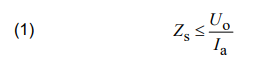
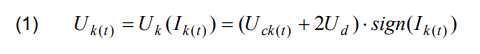
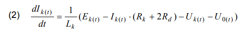
The proposed system uses boost converter which is integrated with the voltage source converter (VSC) [31]. Pulse Width Modulation (PWM) technique [32] is used for control pulses for the boost converter. Proportional-Integral-Derivative (PID) controller [33] is used to obtain the current reference for the battery. The power quality issues across the grid side are controlled through VSC in grid connected mode. It also helps in battery charging during this mode. Point of common coupling voltage and frequency issues are controlled in Standalone mode. The availability of the grid is first checked by using passive method which is indicated in eq. (1)-(2)

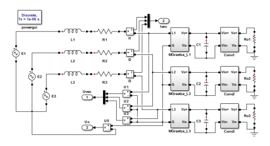
During the availability of the grid, the grid voltage is sensed based on the templates generated by active and reactive power. Fig.3 indicates the schematic approach of the system and Fig. 4 provides the simulated diagram of the system. The proposed system uses Lease Mean Square (LMS) adaptive control algorithm in order to reduce power quality issues in the grid side. Voltage source converter are divided into two major subparts which as unit template estimation (ut) and terminal voltage estimation (Vt). Unit template estimation is calculated using template voltage (Vt) and grid voltage (vg) which is indicated in eq. (3)–(4).


The flowchart of the MPPT algorithm is shown in Fig.5 which provides the switching operation of T1.The gating pulses for the switches S1-S4 for voltage source converter are generated by comparing the reference VSC current with actual VSC current.
Fig.6 indicates the simulated Phase-Locked Loop (PLL) circuitry done using MATLAB software and Fig.7 shows the simulated PID controller for tuning the system. Table 1 provides the information about the simulated specifications carried for the proposed system.

Table 1. System Specifications


The test results in Fig. 8 confirm the transmission of active energy from the battery side to the grid side. The test results include grid power (Pg), load power (PL) and photovoltaic solar energy. (Ppv), power supply VSC (Pvsc). The reactive power of the load is provided by the VSC, and the reactive power of the network is regarded as zero, so the system maintains a power factor of 1. As shown in Fig. 9, in the system under non-linear load, the THD of the line current is 5.2%, while the THD of the VSC current and the THD of the load current are 15.8% and 23.4%, respectively. Thus, the simulation results comply with power quality standard of IEEE 519.
An improved photovoltaic system with a single-phase grid based on the least squares method was implemented, and tests were conducted for various changes in solar radiation and load. The convergence speed of the proposed algorithm is higher than that of the standard LMS algorithm.
Conclusion
In the grid-connected mode and the islanded mode, the single-stage control of the micro-grid based on photovoltaic cells is introduced. The proposed control scheme makes it possible to control the photovoltaic field in the MPPT independently of the presence or absence of the network without using a special boost converter for the photovoltaic field. The analysis is only done in simulation from MATLAB/Simulink and the performance of the system looks to be satisfactory when connected with the grid.
REFERENCES
[1] K. M. Son, K. Lee, D. Lee, E. Nho, T. Chun and H. Kim, “Grid interfacing storage system for implementing microgrid”, 2009 Transmission & Distribution Conference & Exposition: Asia and Pacific, Seoul, Korea (South), (2009), 1-4
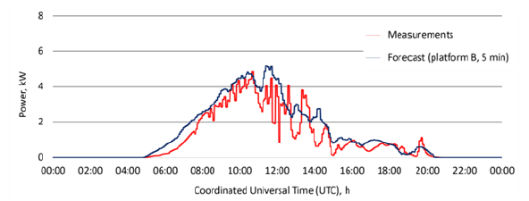
[2] Marcin KOPYT. “Power Flow Forecasts: A Status Quo Review. Part 1: RES Generation Prediction”, PRZEGLĄD ELEKTROTECHNICZNY, 96 (2020), No. 11, 1-4
[3] Bingbing Shao, Shuqiang Zhao, Yongheng Yang, Benfeng Gao, Frede Blaabjerg, “Sub-Synchronous Oscillation Characteristics and Analysis of Direct-Drive Wind Farms With VSC-HVDC Systems”, IEEE Transactions on Sustainable Energy, 12 (2021), No. 2, 1127-1140
[4] Chengshuai Wu, Jian Chen, Chenfeng Xu, Zhiyang Liu, “RealTime Adaptive Control of a Fuel Cell/Battery Hybrid Power System With Guaranteed Stability”, IEEE Transactions on Control Systems Technology, 25 (2017), No. 4, 1394-1405
[5] Hanyu Yang, Canbing Li, Mohammad Shahidehpour, Cong Zhang, Bin Zhou, Qiuwei Wu, Long Zhou, “Multistage Expansion Planning of Integrated Biogas and Electric Power Delivery System Considering the Regional Availability of Biomass”, IEEE Transactions on Sustainable Energy, 12 (2021), No.2, 920-930
[6] Zhijun Wang, Jian Xiong, Xiaoyu Wang, “Investigation of Frequency Oscillation caused False Trips for Biomass Distributed Generation”, IEEE Transactions on Smart Grid, 10 (2019), No. 6, 6092-6101
[7] Muhammad Naveed Akhter, Saad Mekhilef, Hazlie Mokhlis, Noraisyah Mohamed Shah, “Review on forecasting of photovoltaic power generation based on machine learning and metaheuristic technique”, IET Renewable Power Generation, 13 (2018), No. 7, 1009-1023
[8] Belgacem AIS,Tayeb ALLAOUI, Abdelkader CHAKER, Abderrahmane HEBIB, Belkacem BELABBAS, Lalia MERABET, “Contribution to the optimization and control of a Photovoltaic system connected to the Grid based a five levels inverter”, PRZEGLĄD ELEKTROTECHNICZNY, 96 (2021), No. 11, 70-74
[9] Andrzej LANGE1, Marian PASKO, “Selected aspects of photovoltaic power station operation in the power system”, PRZEGLĄD ELEKTROTECHNICZNY, 96 (2020), No. 5, 30-34
[10] Hari Agus Sujono, Riny Sulistyowati, Chairul Anam, Ariadi, Heri Suryoatmojo, “Quadratic Boost Converter with Proportional Integral Control in the Mini Photovoltaic System for Grid”, PRZEGLĄD ELEKTROTECHNICZNY, 96 (2020), No. 6, 47-53
[11] Shatakshi, B. Singh and S. Mishra, “Dual mode operational control of single stage PV-battery based microgrid,” 2018 IEEMA Engineer Infinite Conference (eTechNxT), New Delhi, India, (2018), 1-5
[12] Michal IVANČÁK, Michal KOLCUN, Zsolt ČONKA, Dušan MEDVED, “Modelling microgrid as the basis for creating a smart grid model”, PRZEGLĄD ELEKTROTECHNICZNY, 95 (2019), No. 8, 41-43
[13] B. Singh, K. Kant, A. Chandra and K. Al-Haddad, “Design and implementation of single voltage source converter based standalone microgrid”, 2014 IEEE PES General Meeting | Conference & Exposition, National Harbor, MD, USA, (2014), 1-5
[14] S. Kumar and B. Singh, “Optimum Filtering Theory Based Control for Grid Tied PV-Battery Microgrid System,” 2018 IEEE International Conference on Power Electronics, Drives and Energy Systems (PEDES), Chennai, India, (2018), 1-5
[15] V. Narayanan, S. Kewat and B. Singh, “Standalone PV-BESDG Based Microgrid with Power Quality Improvements”, 2019 IEEE International Conference on Environment and Electrical Engineering and 2019 IEEE Industrial and Commercial Power Systems Europe (EEEIC / I&CPS Europe), Genova, Italy, (2019), 1-6
[16] G. Wu, S. Ishida and H. Yin, “DC Voltage Stabilization in DC/AC Hybrid Microgrid by Cooperative Control of Multiple Energy Storages”, 2019 IEEE Third International Conference on DC Microgrids (ICDCM), Matsue, Japan, (2019), 1-5
[17] T. Lahlou, S. Ramakrishnan, M. Herzog, I. Bolvashenkov and H. Herzog, “A Fast-transient Current Control Strategy for Three-phase Four-wire Modular Multilevel Inverter in Grid-tied Battery Energy Storage System”, 2019 Fourteenth International Conference on Ecological Vehicles and Renewable Energies (EVER), Monte-Carlo, Monaco, (2019), 1-9
[18] S. D, J. G. R, P. K, N. A. A, S. D and N. S, “Symmetrical and Asymmetrical Multilevel Inverter with configurational parameters for power quality applications”, 2020 IEEE 7th Uttar Pradesh Section International Conference on Electrical, Electronics and Computer Engineering (UPCON), Prayagraj, India, (2020), 1-5
[19] R. Ramkumar, M. V. Kumar and D. Sivamani, “Fuzzy Logic based Soft Switched Active Clamped Boost Converter Charging Strategy for Electric Vehicles”, 2020 4th International Conference on Electronics, Communication and Aerospace Technology (ICECA), Coimbatore, India, (2020), 1334-1339
[20] X. Wang, Y. Zheng and Z. Lu, “Simulation Research on the Operation Characteristics of a DC Microgrid”, 2019 IEEE Third International Conference on DC Microgrids (ICDCM), Matsue, Japan, (2019), 1-4
[21] J. Hofer, B. Svetozarevic and A. Schlueter, “Hybrid AC/DC building microgrid for solar PV and battery storage integration”, 2017 IEEE Second International Conference on DC Microgrids (ICDCM), Nuremburg, Germany, (2017), 188-191
[22] B. Singh, B. K. Panigrahi and G. Pathak, “Control of windsolar microgrid for rural electrification,” 2016 IEEE 7th Power India International Conference (PIICON), Bikaner, India, (2016), 1-5
[23] V. Narayanan, Seema and B. Singh, “Solar PV-BES Based Microgrid System with Seamless Transition Capability”, 2018 2nd IEEE International Conference on Power Electronics, Intelligent Control and Energy Systems (ICPEICES), Delhi, India, (2018), 722-728
[24] S. Kumar, B. Singh, U. Kalla, S. Singh and A. Mittal, “Power Quality Control of Small Hydro-PV Array and Battery Storage Based Microgrid for Rural Areas”, 2021 International Conference on Sustainable Energy and Future Electric Transportation (SEFET), Hyderabad, India, (2021), 1-6
[25] Seema and B. Singh, “Intelligent control of SPV-battery-hydro based microgrid”, 2016 IEEE International Conference on Power Electronics, Drives and Energy Systems (PEDES), Trivandrum, India, (2016), 1-6
[26] Maitra and D. Debnath, “A Transformerless Doubly Boost DCDC Converter for grid connected solar photovoltaic systems”, 2018 8th IEEE India International Conference on Power Electronics (IICPE), (2018), 1-6
[27] T. Shanthi and N. Ammasai Gounden, “Power electronic interface for grid-connected PV array using boost converter and line-commutated inverter with MPPT”, 2007 International Conference on Intelligent and Advanced Systems, (2007), 882-886
[28] K. Tabaiya, W. Lenwari and C. Prapanavarat, “A SinglePhase Grid-Connected Inverter Using a Boost Two-Cell Switching Converter with Maximum Power Point Tracking Algorithm”, 2008 5th International Conference on Electrical Engineering/Electronics, Computer, Telecommunications and Information Technology, (2008), 1001-1004
[29] Said AZZOUZ, Sabir MESSALTI, Abdelghani HARRAG, “Innovative PID-GA MPPT Controller for Extraction of Maximum Power From Variable Wind Turbine”, PRZEGLĄD ELEKTROTECHNICZNY, 95 (2019), No. 8, 115-120
[30] Amina ECHCHAACHOUAI, Soumia EL HANI, Ahmed HAMMOUCH, “Comparison of three estimators used in a sensorless MPPT strategy for a wind energy conversion chain based on a PMSG”, PRZEGLĄD ELEKTROTECHNICZNY, 94 (2018), No. 3, 18-22
[31] Kanitphan BOONSOMCHUAE, Satean TUNYASRIRUT, “DSVPWM with Open-leg Switching State for Two-Level Three-Phase Voltage Source Inverters”, PRZEGLĄD ELEKTROTECHNICZNY, 96 (2020), No. 10, 25-31
[32] Priya R Krishnan, Remya Gopalakrishnan, R. Nishanth, Abin
John Joseph, Agath Martin, Nidhin Sani, “PSO-RBFNN based optimal PID controller and ANFIS based coupling for Fruits Drying System”, EAI Transactions on Energy Web, 8 (2021), No. 15, 1-9
[33] Safwan A. Hamoodi, Farah I. Hameed, Ali N. Hamoodi, “Pitch Angle Control of Wind Turbine Using Adaptive Fuzzy-PID Controller”, EAI Transactions on Energy Web, 7 (2020), No. 28, 1-8
Authors: Sudhakiran Ponnuru, Research Scholar, Department of Electrical Engineering, Annamalai University, Chidambaram, Tamilnadu, India, sudhakiran.pon.annamalai@gmail.com
Ashok Kumar R, Professor, Department of Electrical Engineering, Annamalai University, Chidambaram, Tamilnadu, India, ashokraj_7098@rediffmail.com
Jothi Swaroopan NM, Professor, Electronics and Instrumentation Engineering, RMK Engineering college, Chennai, Tamilnadu, India, jothi.eee@rmkec.ac.in
Source & Publisher Item Identifier: PRZEGLĄD ELEKTROTECHNICZNY, ISSN 0033-2097, R. 97 NR 9/2021. doi:10.15199/48.2021.09.26