Published by Ľubomír BEŇA1, Paweł KUT2, Rzeszow University of Technology, Faculty of Electrical and Computer Engineering (1) Rzeszow University of Technology, Faculty of Civil and Environmental Engineering and Architecture (2)
Abstract. The large number of wind farms in the power system makes it possible to use them in the process of voltage regulation in the nodes to which they were connected. The regulation possibilities depend on the generators in which the wind farm has been equipped. Currently, Doubly-Fed Induction Generators are the most commonly used ones, which have wide possibilities of reactive power and voltage control at the wind farm connection point. The article presents an analysis of the connection of a wind farm consisting of wind turbines equipped with DFIG generators to the power system for the possibility of voltage regulation. Simulations were carried out using PowerWorld Simulation software.
Streszczenie. Duża liczba farm wiatrowych w systemie elektroenergetycznym stwarza możliwość wykorzystania ich w procesie regulacji napięcia w węzłach do których zostały przyłączone. Możliwości regulacyjne zależą od generatorów w jakie zostały wyposażone elektrownie wiatrowe. Obecnie najczęściej znajdują zastosowanie generatory asynchroniczne dwustronnie zasilane, które posiadają szerokie możliwości regulacji mocy biernej, a co za tym idzie napięcia w punkcie przyłączenia farmy wiatrowej. W artykule przedstawiono analizę przyłączenia farmy wiatrowej, składającej się z elektrowni wiatrowych wyposażonych w generatory asynchroniczne dwustronnie zasilane do systemu elektroenergetycznego pod kątem możliwości regulacji napięcia. Symulacje zostały przeprowadzone z wykorzystaniem oprogramowania PowerWorld Simulator. Farmy wiatrowe w procesie regulacji napicia w systemie energetycznym
Keywords: wind farm, voltage, reactive power, power system Słowa kluczowe: farma wiatrowa, napięcie, moc bierna, system elektroenergetyczny
Introduction
Renewable energy sources are now considered to be the most prospective energy sector. Solar energy and its derivatives are a free and inexhaustible source of energy [1]. Thanks to the rapid development of technologies in the field of renewable energy, the efficiency of generating units increase year by year, while the investment cost decrease. Increasing the share of renewable energy sources in the energy systems of the Member States is now a priority in the European Union energy policy. Funds earmarked for this purpose are to accelerate the development of renewable energy sources and enable diversification of fuels and gradual independence from conventional fuels. The current climate package assumes an increase in renewable energy sources share in the European Union to 20% by 2020. In 2016, the share of renewable energy in final energy consumption was 17% for the European Union [2]. Another target will be to increase energy production in renewable energy sources to 27% in 2030 [3].
According to the data of the Polish Energy Regulatory Office [4], in the Polish national power system, the total installed capacity in renewable energy sources at 30.05.2018 amounted to 8 584,552 MW, and the power in installations using wind energy was 5 874,778, which is 68,43% of the total installed power in renewable energy. One can notice the slowdown in the development of wind energy in Poland as a result of the Wind Farm Investment Act [5,6]. In 2016, the installed capacity in wind sources was 5 807,416 MW, so within 2 years the power increased by only 67,362 MW.
The high installed capacity in wind farms makes it possible to use them for the process of voltage regulation in the power system nodes. Thanks to the use of wind farms with large reactive power control options, the transmission system operator can use wind farm to maintain the required voltage level at the connection point [7]. The use of wind farms in the reactive power control process also allows limiting voltage fluctuations resulting from the stochastic nature of wind and reducing power losses in the internal network of the wind farm and in the network to which it is connected. The connection of wind farms to the power system does not increase the voltage distortion at the connection point [8].
Voltage in the power system
To ensure correct operation of the power system, it is necessary to balance the active and reactive power. One of the basic parameters affecting the quality of electricity is frequency and voltage. Maintaining a constant frequency requires balancing of active power, while a proper balancing of reactive power is associated with maintaining the correct voltage in the system nodes.
The demand of receiving nodes for reactive power is around 42%. The remaining 58% are own needs of the network, which include: longitudinal losses in lines – 21%, longitudinal losses in transformers – 20%, generators demand – 9% and losses in network transformers – 8% [9].
Constant changes in the system load make it necessary to adjust the voltage levels in the power system nodes. Voltage deviations below the rated value are caused by [10]:
• voltage drops in medium and low voltage lines and in transformers;
• too low voltage on the medium voltage side in station 110/MV, resulting from fault conditions. Voltage deviations above the rated value are caused by:
• positive value of longitudinal voltage loss induced by capacitive reactive power flows;
• too high voltage on medium voltage substation bus and MV/LV transformers in abnormal operating conditions.
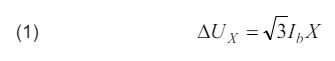
The value of voltage drop in overhead lines and transformers depends primarily on the part of the longitudinal voltage loss, which is dependent on the reactive component of the current:
.
where: Ib – reactive component of the current.
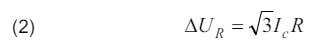
The longitudinal part of the voltage loss depends on the active current component is much smaller:
.
where: Ic– active component of the current.
This is due to the fact that the value of the overhead line reactance is much higher compared to the resistance. The longitudinal voltage loss increases the value of the voltage at the end of the line when capacitive and less at inductive. For this reason, voltage regulation is closely related to the reactive power regulation.
Wind turbines equipped with an Doubly-Fed Induction Generator
Wind turbines equipped with DFIG (Doubly-Fed Induction Generator) generators have a wide range of active and reactive power regulation, which is why they currently belong to the most commonly used generators in wind energy sector. DFIG generators allow to obtain better quality of electricity compared to other generators used in wind farms. They provide active suppression of voltage and power oscillations as well as current and voltage harmonics.
Doubly-Fed Induction Generators are equipped with an energy electronic converter connected to the rotor circuit, thanks to which it is possible to transmit energy in both directions: from and to the rotor [11]. DFIG generators enable operation at both super-synchronous and sub-synchronous speeds. In the case of super-synchronous operation, the energy flows from the rotor to the grid, while during the work with the sub-synchronous speed, the energy flows from the stator to the rotor.
Figure 1 shows the characteristics of the Vestas V90 – 3 MW wind turbine equipped with Doubly-Fed Induction Generator, on which the area of permissible operating conditions is marked.
Fig.1. Area of permissible operating conditions of the DFIG generator at Vestas V90 – 3 MW wind turbine [12]
Wind turbines Vestas V90 – 3 MW enable operation in the constant power factor mode in the range of 0,98cap – 0,96ind. It is possible to work with a different power factor, but with a reduction in the value of active power generated. When generator is connected in a triangle, the maximum reactive power generated is 1500 kvar, while for star connection 750 kvar.
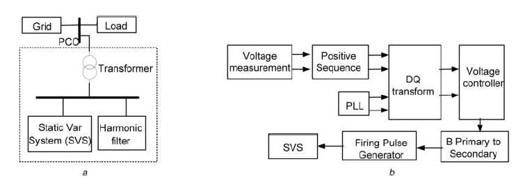
Analysis of the possibility of using a wind farm in voltage regulation
Simulations were carried out using the PowerWorld Simulator program. PowerWorld Simulator enables analysis of active and reactive power distribution as well as voltage level analysis in power system nodes.
The analysis of the wind farm’s impact on the voltage level in the power network was carried out for a wind farm consisting of 10 wind turbines Vestas V90 – 3 MW (Fig.2, EW1-EW10). The 30 MW wind farm was connected to the 110 kV network.
Figure 2 shows the diagram of the internal network. The wind farm has a three radial lines connected to the main supply point located on the wind farm. In the case of a radial structure, damage to the cable stops the transmission of energy from wind turbines located behind the damaged part of the internal network. The ring topology is characterized by greater reliability, but requires higher investment costs.
Fig.2. Diagram of the internal network of the analyzed wind farm
The diagram of the analyzed fragment of the power system, modelled in the PowerWorld Simulator is shown in figure 3. The wind farm was connected at node 13.
Fig.3. Diagram of the analyzed fragment of the power system
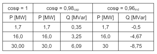
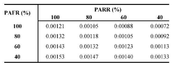
Table 1 presents the values of active and reactive power of a wind farm for which simulations have been carried out. Reactive power was determined based on the simulation of the internal network of the wind farm.
Table 1. The values of active and reactive power in simulations
.
Figure 4 shows the results of the simulation depending on the power factor of wind farms.
Fig.4. Relation between the voltage in the nodes and generated active power by wind farm for: cosφ = 1(a), cosφ = 0,98cap (b), cosφ = 0,96ind (c)
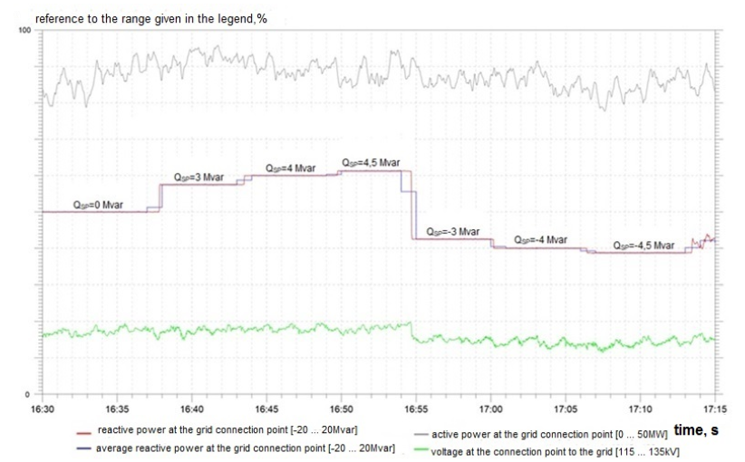
The regulations possibilities of a wind farm consisting of wind turbines equipped with Doubly-Fed Induction Generators, create the possibility of improving voltage conditions in the node to which the wind farm is connected and in neighbouring nodes. In case the voltage at the connection point is lower than required, the wind farm may became a source of reactive power, which will increase the voltage in the node. In the analyzed case, when wind turbines operate with a power factor of cosφ = 0,98cap, the voltage at the connection point (node 13), compared to work with the power factor cosφ = 1, increased by 0,9% for a wind farm working with 30 MW. In the case of wind turbines operating with a power factor cosφ = 0,96ind, it is possible to obtain a constant voltage in the nodes, despite increasing the active power generation. Figure 5 shows relation between voltage and reactive power.
Fig.5. Relation between voltage and reactive power for: P = 30 MW (a), P = 1,76 MW (b)
Figure 6 shows the power losses in the analyzed fragment of the power system depending on the active power for the analyzed values of the power factor cosφ.
Fig.6. Relation between active power losses in the network and generated active power
In the case of wind turbines with cosφ = 0,98cap, the losses of active power in the network to which the farm is connected are reduced as compared to the work with the power factor cosφ = 1.
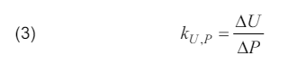
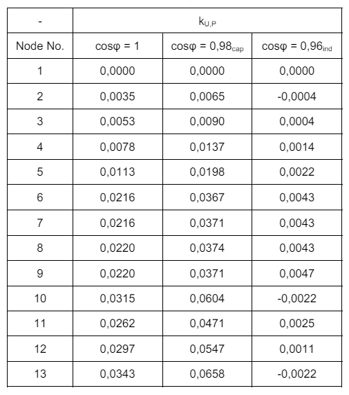
Table 2 shows the calculated coefficient kU,P, which is a measure of how the voltage in the network nodes changes depending on the active power generated. The higher value of this coefficient means the greater difference between the voltage in the node depending on the generated active power. The coefficient kU,P is defined by the formula:
.
where: ∆U – voltage difference, ∆P – difference between maximum and minimum active power generated by wind farm.
.
Table 2. Values of the coefficient kU,P
.
As can be seen from the above results, increasing the reactive power output increases the voltage at all nodes of the network.
Summary
Wind farms, thanks to their regulation capabilities, can be used by the transmission system operator to regulate the voltage in the node to which it was connected and in neighbouring nodes.
The ability to work with reactive power capacitive and inductive by wind turbines with Doubly-Fed Induction Generators allows to maintain a constant voltage at the connection point despite increasing the active power generation and increasing or decreasing the voltage in the node.
The connection of wind farms close to the recipients also positively influences the level of active power losses in the network, which decreases when the wind farm work with higher active power.
REFERENCES
[1] Proszak-Miąsik D., Bukowska M., Nowak K., Rabczak S., Astronomical and meteorological conditions of a solar system operation, Iop Conf Ser-Mat Sci., 245, (2017) [2] Statistical data on energy from renewable sources, Eurostat [3] http://www.cire.pl/item,96778,1,0,0,0,0,0,ke-do-2030-r-wzrostefektywnoscienergetycznej-o-30-proc.html, Dostęp. 01.12.2018 [4] http://www.ure.gov.pl/pl/rynki-energii/energiaelektryczna/odnawialne-zrodla-ener/potencjal-krajowyoze/5753,Moc-zainstalowana -MW.html, dostęp 01.12.2018 [5] Ustawa z dnia 20 maja 2016 r. o inwestycjach w zakresie elektrowni wiatrowych [6] Ustawa z dnia 7 czerwca 2018 roku. o zmianie ustawy o odnawialnych źródłach energii oraz niektórych innych ustaw [7] Pijarski P., Kacejko P., Wancerz M., Gryniewicz-Jaworska M., Układ sterowania mocą bierną farmy wiatrowej wykorzystujący możliwości regulacyjne przekształtników, dławika zaczepowego oraz pojemność kabla zasilającego farmę, Przegląd Elektrotechniczny, 92 (2016), nr. 8, 44-47 [8] Gała M., Praca turbin wiatrowych w systemie elektroenergetycznym oraz ich wpływ na jakość energii elektrycznej, Przegląd Elektrotechniczny, 93 (2017), nr.6, 37-40 [9] Kot A., Bilans I zapotrzebowanie mocy biernej w Krajowym Systemie Elektroenergetycznym, Acta Energetica, 1 (2013), nr.14, 68-71 [10] Praca zbiorowa, Poradnik inżyniera elektryka, WNT, 2011 [11] Klucznik J, Udział farm wiatrowych w regulacji napięcia w sieci dystrybucyjnej, Acta Energetica, 1 (2010), nr. 3, 39-39 [12] Grządzielski I., Sposoby kompensacji mocy biernej, prezentacja Międzynarodowe Targi Energetyki Expopower, Poznań 2010.
Authors: dr hab. inż. Ľubomír Beňa, prof. PRz, Rzeszow University of Technology, Faculty of Electrical and Computer Engineering, Department of Power Electronics and Power Engineering, ul. Wincentego Pola 2, 35-959 Rzeszów, E-mail: lbena@prz.edu.pl; mgr inż. Paweł Kut, Rzeszow University of Technology, Faculty of Civil and Environmental Engineering and Architecture, Department of Heat Engineering and Air Conditioning, Al. Powstańców Warszawy 6, 35-959 Rzeszów, E-mail: p.kut@prz.edu.pl.
Source & Publisher Item Identifier: PRZEGLĄD ELEKTROTECHNICZNY, ISSN 0033-2097, R. 95 NR 8/2019. doi:10.15199/48.2019.08.33
Published by Joanna KOZIEŁ, Grzegorz KOMARZYNIEC, Andrzej WAC-WŁODARCZYK, Ryszard GOLEMAN, Department of Electrical Engineering and Electrotechnologies, Lublin University of Technology
Abstract. The article presents the characteristics of the net power of a wind farm as a function of wind speed, and lists the factors determining the selection of a wind farm. Classification of large wind turbine generators is illustrated. The work areas of a synchronous, 3-phase generator with permanent magnets are depicted. Responses of a given wind farm to the demand for capacitive and inductive reactive power are presented.
Streszczenie. W artykule przedstawiono charakterystykę mocy netto farmy wiatrowej w funkcji prędkości wiatru, oraz wymieniono czynniki decydujące o wyborze farmy wiatrowej. Zilustrowano klasyfikację generatorów dużych turbin wiatrowych. Zobrazowano obszary pracy generator synchronicznego, 3-fazowego z magnesami trwałymi. Przedstawiono odpowiedzi określonej farmy wiatrowej na zapotrzebowanie na moc bierną o charakterze pojemnościowym, jak i indukcyjnym. (Analiza wpływu farmy wiatrowej na jakość energii elektrycznej w sieci dystrybucyjnej).
Keywords: wind farm, farm location, permanent magnet 3-phase synchronous generator, reactive power. Słowa kluczowe: farma wiatrowa, lokalizacja farmy, generator synchroniczny 3 fazowy z magnesami trwałymi, moc bierna.
Introduction
A specific feature of electricity is that, in terms of certain parameters, its quality is more influenced by the user than the producer or system operator. In these cases, the system user is the basic partner of the system operator in the efforts to maintain the proper quality of electricity.
It should be noted that these problems are dealt with in other standards already published or in development. The emission standards define the levels of electromagnetic disturbances which can be caused by the devices of the system users. Immunity standards set levels of disturbance that devices can tolerate without undesirable damage or loss of function. The third set of standards for electromagnetic compatibility [1],[2] levels allows the emission standards and immunity standards to be coordinated and coherent in such a way as to achieve the overarching goal of electromagnetic compatibility [3].
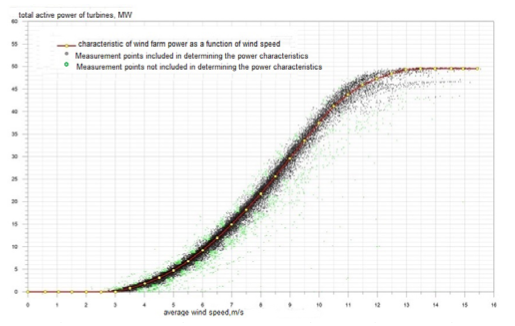
Fig.1. Characteristics of the net power of a wind farm as a function of wind speed
Modern wind turbines usually have a horizontal axis of rotation, and the turbine itself usually has three blades. The vast majority of turbines are equipped with asynchronous generators [4].
The wind pressure on the blades creates a pressure difference in front of and behind the blades. The turbine begins to rotate and the rotor drives a generator located in the nacelle. It is in the generator that the mechanical energy is converted into electricity. The rotational speed of a typical asynchronous generator oscillates around 1500 rpm, which requires the use of a gear located between the rotor and the generator [4].
A wind farm – also known as a wind power plant, is a group of wind turbines equipped with generators, generating electricity, powered by wind power. The energy obtained in this way is referred to as “clean” energy, because during its production the turbine does not emit pollutants related to fuel combustion.
The actual net power recorded at the transformer terminals, depending on the wind speed, is shown in Fig. 1.
Factors determining the location of the wind farm
Choosing the right location of the facility is crucial for the success of a given investment, therefore it is necessary to thoroughly analyse all factors [5]. In the case of wind farms one should:
• ensure the access of the wind farm to the National Power System, • keep the required distances between the turbines and arrange them in such a way as to make the most efficient use of production capacity, • exclude protected areas, areas of national parks and nature reserves, • exclude areas adjacent to airports, railways, expressways, • keep appropriate distances from human clusters, • keep the statutory distances from transmission lines, e.g. high voltage and oil and gas pipelines, • ensure compliance with applicable legal acts, including environmental guidelines.
However, the most important determinant of the location is the average wind speed for a given area during the year. It depends on the wind speed whether the wind farm will be able to produce enough energy to make the investment profitable. And so, on the basis of data collected at over 60 stations throughout the country, average wind speeds were determined for given areas [5], [6].
It should be noted that winter is the windiest period, therefore the most desirable and generating the largest amounts of energy produced by wind farms.
Wind speed is a decisive factor in the ability to produce and regulate energy in the distribution system. For an exemplary Vestas V112 turbine is use in this farm. The limiting wind speed at which the Vestas V112 turbine starts producing electricity is 3 m/s. According to the characteristics, it is the equivalent of the production of 22 kW of active power. The critical speed can also be read from the characteristics of the turbine. For this wind turbine model it is 25 m/s. Above this wind speed, the turbine will stop. As it is easy to read from the diagram, the turbine already reaches the rated power of 3.3 MW at a speed of about 13 m/s. In the event of winds blowing at speeds below 3 m/s, as recommended by both the wind farm operators and the turbine manufacturer, the turbine should be stopped. Restarting it is often problematic, e.g. in winter, when ice blocks can form on the blades. In order to prevent this, turbines are usually not stopped in such cases, but instead take power from the power grid and drive the rotor (they work by drawing power from the National Power System).
Table 1. Summary of wind speed for various time periods
.
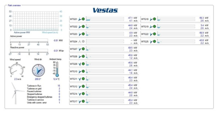
Fig.2. A photo of the panel visible to the wind farm worker
Fig.3. Area of achievable states of a synchronous generator operating in a power plant, connected directly to the grid (blue, red and black lines) and wind farms (brown line)
On a day when low wind speed prevails, the wind farm draws power from the grid to drive the wind turbines. The appearance of the wind farm SCADA system panel is shown in Figure 2. Despite the use of automation, it is a simpler method of control, because the start-up of wind turbines is associated with a certain risk, resulting from a power outage for the electronics in the nacelle. As can be seen, the WTG04 turbine is stopped due to some error. The farm automation has the ability to constantly interfere with the operation of wind turbines (load change, regulation change, setting angle in relation to the wind direction, starting or stopping the turbine operation). Probably due to an error or in time to repair the operation of the turbine was stopped. The remaining turbines draw their active power from the grid. For example, the WTG07 turbine draws 69.5 kW of power, and the wind speed measured at the top of its nacelle is 2.3 m/s. These are instantaneous values, refreshed by the system at regular intervals.
Each of the turbines operates at wind speeds below 3 m/s. For this reason, turbines need power from the grid to operate. It seems that only the WTG04 turbine does not draw power from the grid, but it is the turbine whose operation in the wind farm system has been suspended.
Regulation of voltage and reactive power of a wind farm in the power grid
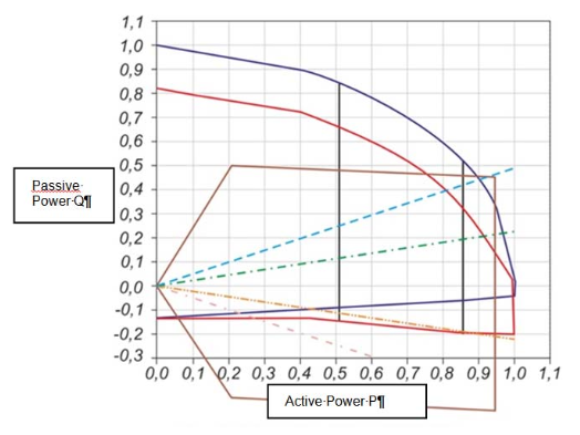
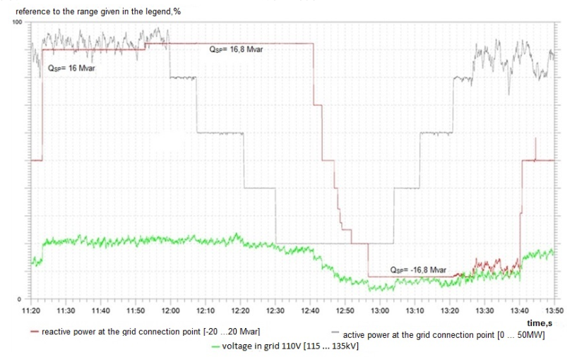
The participation of wind turbines in the process of voltage regulation in the power grid is strictly dependent on their ability to generate reactive power. It results directly from the areas of turbine operating states. Modern wind farms are adapted not only to the production (generation) of reactive power, but also to its consumption from the grid. The common ones include wind farms with characteristics similar to a triangle, or more often to a polygon. The reactive power generation capabilities of such farms are large and reach up to 50% of the rated active power. Unfortunately, for small values of wind farm power, there is a close dependence of the generated active power on reactive power (Fig. 3) [7], [8], [9]. Nevertheless, the reactive power regulation function is very important from the point of view of the voltage stability of the system. In order to take a closer look at the above issue, the division of generators used in large wind turbines should be considered. Classification of large wind turbine generators : Large wind turbine generators,
• Induction (asynchronous) generators, • Synchronous generators, • Double-fed induction generators, • Cage induction generators, • Generators with wound rotors, • Generators with permanent magnets, • Generators with slip ring-powered rotors, • Generators with brushless rotors, • Generators with embedded magnets, • Generators with surface-mounted magnets.
The generators most often used in wind turbines include a synchronous three-phase generator with permanent magnets. The areas of its work are presented in Figure 3.
The characteristics of a classic generator block, defined at the level of the generator busbars, are marked in red. The blue colour is the characteristic of the upper voltage of the block transformer. The black lines, in turn, limit the minimum and maximum value of the active power generated by the steam turbine.
This is due to the generation limitations of this turbine and boiler. Wind turbines are an excellent source of energy, as shown in Figure 3. The working area is wide. Wind farms can operate with a higher reactive power consumption while simultaneously having small active power generations. Unfortunately, for low values of the generated active power, this range is very limited and so, most of the time during the year, there is uncertainty as to the possibility of obtaining reactive power at all [10],[11]. Wind farm responses to the demand for capacitive and inductive reactive power are presented in Figure 4.
Fig.4. The regulation system working in the reactive power regulation mode
Fig.5. Characteristics of Q = f (t) of a wind farm
Conclusions
Wind farms have a significant impact on the regulation of voltage parameters in the power grid. The appropriate location of the wind farm has a decisive influence on the regulatory possibilities of the wind farm. The potential of wind farms has been noticed and they are undoubtedly becoming an important element supporting the regulation of the National Power System. Regulatory capacity of wind farms is not applicable to less developed energy systems, e.g. island systems. The wind farms can regulate the frequency and active power, voltage and reactive power, resulting in a constant power factor cosφ. Wind farms are able to react quickly to grid disruptions thanks to their power reserve.
REFERENCES
[1] Michałowska J., Mazurek P.A., Gad R., Chudy A., Kozieł J., Identification of the electromagnetic field strength in public spaces and during travel, 2019 Applications of Electromagnetics on Modern Engineering and Medicine PTZE 2019, pp.121-124, 8781737. [2] Mazurek P.A., Michałowska J., Kozieł J., Gad R., Wdowiak A., The intensity of the electromagnetic field in the coverage of GSM 900, GSM 1800, DECT, UMTS, WLAN in build – up areas, 2018 Applications of Electromagnetics on Modern Engineering and Medicine PTZE 2018, pp. 159-162, 8503156. [3] Norma EN 50160:2010 [4] Wolańczyk F,. Elektrownie wiatrowe, Wydawnictwo KaBe, Krosno 2013 [5] Dygulska A., Perlańska E., Mapa wietrzności Polski, project Czysta Energia, Słupsk, 2015 [6] Montusiewicz J., Gryniewicz-Jaworska M., Pijarski P., Looking for the optimal location for wind farms, Advances in Science and Technology Research Journal, vol. 9, s. 135-142, 2015 [7] Kacejko P., Pijarski P., Gałązka K., Prosument – krajobraz po bitwie, Rynek Energii, vol. 117, nr 2, s. 40-44, 2015 [8] Pijarski P., Wydra M., Kacejko P., Optimal control of wind power generation, Advances in Science and Technology Research Journal, vol. 12, nr 1, s. 9-18, 2018 [9] Zmarzły D., Badania jakości energii w wybranej farmie wiatrowej, Politechnika Opolska, Opole 2014 [10] Kacejko P., Pijarski P., Gałązka K., Prosument – przyjaciel, wróg czy tylko hobbysta, Rynek Energii, vol. 114, nr 5, s. 83- 89, 2014 [11] Pijarski P., Rzepecki A., Wydra M., Efektywne zarządzanie mocą farm wiatrowych, Rynek Energii, vol. 111, nr 2, s. 69-74, 2014
Authors: dr inż. Joanna Kozieł, Department of Electrical Engineering and Electrotechnologies, Faculty of Electrical Engineering and Computer Science, Lublin University of Technology, ul. Nadbystrzycka 38A, 20-618 Lublin, e-mail: j.koziel@pollub.pl; dr hab. inż. Grzegorz Komarzyniec, prof. uczelni, Department of Electrical Engineering and Electrotechnologies, Faculty of Electrical Engineering and Computer Science, Lublin University of Technology, ul. Nadbystrzycka 38A, 20-618 Lublin, e-mail: g.komarzyniec@pollub.pl; prof. dr hab. inż. Andrzej WacWłodarczyk, Department of Electrical Engineering and Electrotechnologies, Faculty of Electrical Engineering and Computer Science, Lublin University of Technology, ul. Nadbystrzycka 38A, 20-618 Lublin, e-mail: a.wacwlodarczyk@pollub.pl; dr hab. inż. Ryszard Goleman, prof. uczelni, Department of Electrical Engineering and Electrotechnologies, Faculty of Electrical Engineering and Computer Science, Lublin University of Technology, ul. Nadbystrzycka 38A, 20-618 Lublin, e-mail: r.goleman@pollub.pl.
Source & Publisher Item Identifier: PRZEGLĄD ELEKTROTECHNICZNY, ISSN 0033-2097, R. 97 NR 12/2020. doi:10.15199/48.2020.12.43
Published by Justyna HERLENDER, Jan IŻYKOWSKI, Eugeniusz ROSOŁOWSKI, Wroclaw University of Science and Technology, Department of Electrical Power Engineering
Abstract. This paper deals with analysis of impedance-differential protection applied to locating faults on power transmission line. Based on the voltage and current measurements at both line ends, the differential impedance is calculated. It enables to formulate efficient protective algorithm. Moreover, the presented impedance-differential protection has ability to determine the fault location for an inspection-repair purpose. The fault signals from ATP-EMTP simulations of faults on the sample transmission line was applied for evaluating the fault location accuracy and to compare with the other fault location methods.
Streszczenie. Artykuł prezentuje analizę impedancyjnego zabezpieczenia różnicowego w zastosowaniu do lokalizacji zwarć w linii przesyłowej. Stosując pomiary napięć i prądów na obu końcach linii wyznaczana jest impedancja różnicowa. Pozwala ona na sformułowanie efektywnego algorytmu zabezpieczeniowego. Ponadto takie zabezpieczenie pozwala na lokalizowanie zwarć do celów inspekcyjno-remontowych. Sygnały zwarciowe z symulacji zwarć w przykładowej linii przesyłowej z użyciem programu ATP-EMTP zastosowano do oceny dokładności lokalizacji i porównania z innymi metodami lokalizacji (Impedancyjne zabezpieczenie różnicowe jako lokalizator zwarć w linii przesyłowej).
Keywords: impedance-differential protection, transmission line, fault location, fault simulation. Słowa kluczowe: impedancyjne zabezpieczenie różnicowe, linia przesyłowa, lokalizacja zwarć, symulacja zwarć.
Introduction
Published fault statistics [1]-[2] unambiguously indicate that majority of total number of power system faults occur on overhead power lines. Such faults have to be detected and then located by protective relays as well as by fault locators [2]. In order to prevent spreading out the fault effects, the identified fault has to be cleared by a circuit breaker tripped by a protective relay as quickly as possible. Improvement of protective relays operation is of concern in many researches performed all over the world. Application of synchronized measurements [3]-[5] appears as one of the means for that purpose. In particular, such measurements allow to get modern differential protection systems of overhead power transmission lines [6]-[8].
This paper deals with impedance-differential relay providing effective protection of transmission lines [7]. The traditional current differential relays [6] apply measurements of three-phase currents at the line ends, while the impedance-differential relay under consideration [7] utilizes the measurements of both currents and voltages from the line ends. Thus, more information on the fault is provided in the case of impedance-differential relay. As a result, effective protection of transmission line is achieved [7]. Moreover, a distance to fault can be determined [9]-[12] which can be utilized for an inspection-repair purpose, i.e., for sending the repair crew to remove the fault and thus allowing the line to be switched on into operation. This paper is analyzing the fault location feature of the impedance-differential relay. In particular, a comprehensive evaluation of fault location accuracy with use of the simulation data is presented.
Impedance-differential protection – formulation for single phase system
Figure 1 presents a simplified single phase model of the transmission line utilized to present the impedance differential protection principle [7]. After deriving the algorithm for such a case then it will be extended to three-phase system.
The line is represented with the lumped impedance (ZL) and the line shunt admittances uniformly distributed:
.
where CLis the line shunt capacitance.
It is assumed that the fault (F) is on the line S-R, at the relative distance d [p.u.], counted from the bus S.
Fig.1. Single phase model of faulted transmission line
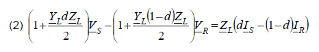
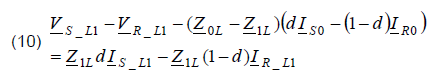
The following expressions can be written for the circuit of Figure 1:
.
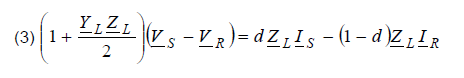
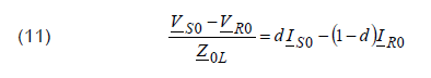
The coefficients at the measured voltage Vs, VR in (2) are different and depend on the distance to fault d. However replacing them by their average value results in:
.
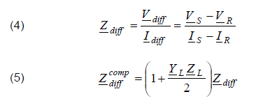
The differential impedance and the compensated differential impedance are introduced as follows:
.
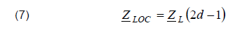
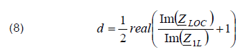
Now the locational differential impedance is defined as:
.
Taking into account (4)-(6) one can obtain that the locational differential impedance is the following function of the sought distance to fault:
.
Therefore the fault location can be performed using
.
At the right-hand side of (8) the real part is taken to reject some imaginary part which can appear due to the calculation errors.
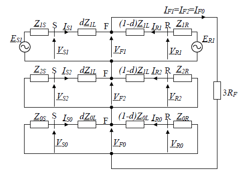
Impedance-differential protection – formulation for three phase system
For the purpose of paper conciseness only calculations of asymmetrical faults are demonstrated here, while the symmetrical faults consideration are presents in [7].
Differential impedance regarding asymmetrical faults can be determined using the symmetrical components. For calculation, in this paper, single-phase-to-earth fault is applied. Figure 2 represents the positive-, negative-, and zero-sequence network for a single phase-to-earth fault.
Fig.2. Interconnection of equivalent networks for positive-, negative- and zero-sequence components under L1-E fault
From Figure 2 following relationships can be observed:
.
Considering that the fault occurs in phase L1, and after implementation of symmetrical component properties, it can be obtained from (9):
.
In view of zero sequence circuit presented in Figure 2, the voltage drop can be formulated as:
.
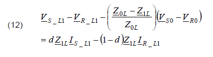
After substituting (11) to (10), the following formula is obtained:
.
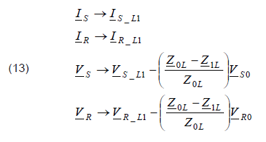
The formula (12) is analogous to (3) which was obtained for a single phase system. Therefore, taking this analogy, one can extend usage of the set of equations (4)-(8) to the single phase fault (L1–E) in three-phase system by taking:
.
Analogous substitutions one has to apply for the remaining single phase faults (L2–E, L3–E). Moreover, this can be applied for phase1-phase2 and phase1-phase2-earth faults as well.
Data of simulated system
For evaluation of the presented protection algorithm, the model of the 400 kV double fed transmission line (Tab. 1) has been tested. The simulation was performed using the ATPDraw [13], while protection algorithm was implemented in MATLAB software. The phasors of measured currents and voltages were determined by the full-cycle Fourier filtering.
Table 1. Parameters of the modeled transmission line
.
Fault resistance influence
Length of the investigated line varied, and was equal to the following values: 80 km, 200 km and 300 km. However, for the sake of briefness, only results for 300 km line are shown in this paper. In order to test the proposed protection algorithm, short-circuit simulations were conducted inside the line as well as beyond it. The inner faults were simulated, referring to the S side at distances of d = 0; 0.1; 0.2; 0.3;…1. The faults applied outside the protected line, were located behind the terminals S and R, respectively. The studies included symmetrical faults (three-phase-to-earth faults) and different asymmetrical faults (phase-to-earth (L1-E), phase-to-phase (L1-L2), and phase-to-phase-to-earth (L1-L2-E) faults).
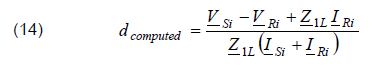
The presented fault location algorithm was compared with the two-end synchronized fault location algorithms (14) presented in [2]
.
where i – kind of processed signals.
The error of studied impedance-differential algorithm was defined as
.
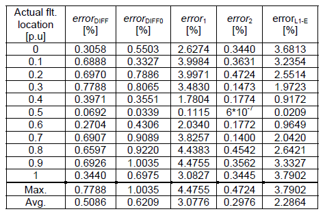
The presented results in Table 2 and 3 concern phase-to-earth (L1-E) faults inside the protected line, regarding to the fault resistance. The results included phase-to-phase faults are presented in Table 4. The fault location errors were determined as follows:
• errorDIFF – use of signals of impedance-differential protection • errorDIFF0 – as for errorDIFF but without shunt capacitances compensation • error1 – use of positive sequence component • error2 – use of negative sequence component • errorL1-E – use of signals applied in distance protection for L1-E fault • errorL1-L2 – use of signals applied in distance protection for L1-L2 fault.
It is visible that fault location computation concerning compensation were more accurate than neglecting it. Maximal error obtained by the presented algorithm (with compensation) did not exceed 0.8% while without compensation this value was insignificantly higher than 1%. In contrast, the result calculated in case of positive sequence component based location algorithm was even greater than 4%.
Additionally, for phase-to-phase faults, the average error computed for considered protection method was equaled to 0.0904% (with compensation) and it means that from all used methods this calculated faults location the most accurately. On the contrary, the average error calculated for negative sequence based algorithm was the highest in case of the faults simulated for fault resistance amount to 2 Ω.
Generally, the differential impedance algorithm enabled to locate faults with maximal average error equaled to 0.5086%. Only algorithm based on negative sequence components worked more accurate, and the maximal average error did not exceed 0.3418%. However, taken into consideration all average error results, differential impedance protection method was the most precise from all of compared algorithms in except of the simulation made for L1-E fault with RF=10 Ω.
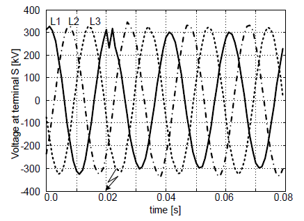
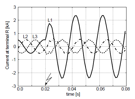
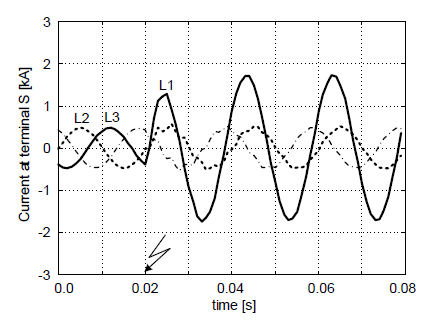
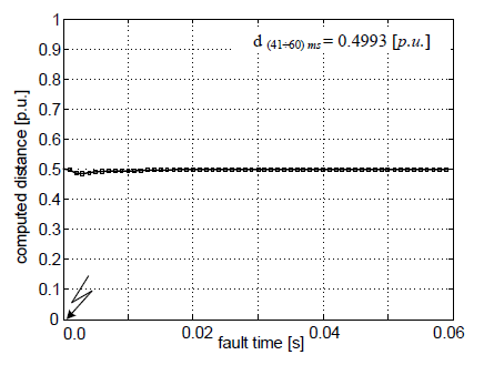
The sample example is presented in Figure 3 – 7. The specifications of it are as follows: phase-to-earth (L1-E) fault at the midpoint of 300 km line, RF=10 Ω. The computed fault location is depicted in Figure 7 where d(41÷60)ms was obtained by averaging within the interval (41÷60) ms after the fault inception.
Fig.3. The example – voltage at terminal R
Fig.4. The example – voltage at terminal S
While simulating short-circuits in the middle of the protected line, it was observed that independently of the applied fault location algorithm, the computed distances were characterized by the smallest error. This situation was observed for all fault types.
As presented in Tables 2 – 4, the considered protection algorithm allows to detect faults in all conditions, regardless of different fault types and fault resistance.
Fig.5. The example – current at terminal R
Fig.6. The example – current at terminal S
Fig.7. The example – computed distance
Conclusions
The aim of this paper is to present the concept of impedance-differential protection for long transmission lines. The demonstrated protection algorithm enables not only for internal fault detection, but can be applied also as a fault locator.
Based on simulation results it can be concluded that presented method can be used for transmission lines with different lengths as well as is not influenced by the fault resistance changes.
Moreover, capacitive charging current which constitutes the main drawback of current differential protection is eliminated in presented protection method and does not influence on the fault location determination.
In addition, the accuracy of fault location achieved in case of impedance-differential relay allows to improve the faults location calculation obtained from the use of two-end synchronized fault location algorithms. The precision of presented algorithm is on the same level as for method using negative sequence components and even has superiority over it, in case of phase-to-phase faults (L1-L2 faults, Tab. 4).
The obtained results approve the high reliability of the impedance-differential protection.
For the further studies of demonstrated protection algorithm as a transmission line fault locator, the impact of source strength or shunt reactors application could be evaluated.
REFERENCES
[1] Kacejko P., Machowski J., Zwarcia w systemach elektroenergetycznych, WNT Warszawa (2002) [2] Saha M.M., Izykowski J., Rosolowski E., Fault Location on Power Networks, Springer, London (2010) [3] Halinka A., Szewczyk M., Talaga M., Metodyka pomiarów synchronicznych (PMU) oraz przykłady zastosowania. Wiadomości Elektrotechniczne, 82 (2014), no 8, 21-25 [4] Iżykowski J., Rosołowski E., Synchroniczne pomiary rozproszone w zastosowaniu do lokalizacji zwarć w liniach napowietrznych, Przegląd Eektrotechniczny, 85 (2009), no. 11, 21-25 [5] Szewczyk M., Time synchronization for synchronous measurements in Electric Power Systems with reference to the IEEE C37.118TM Standard – selected tests and recommendations, Przegląd Elektrotechniczny, 91 (2015), no. 4, 144–148 [6] Altuve Ferrer H.J., Kasztenny B., Fischer N., Line current differential protection, A collection of technical papers representing modern solutions, Schweitzer Engineering Laboratories, (2014) [7] Ghanizade Bolandi T., Seyedi H., Hasemi S.M., Soleiman Nezhad P., Impedance-differential protection: A new approach to transmission-line pilot protection, IEEE Transaction on power delivery, 30 (2015), no. 6, 2510-2518 [8] Suonan J.L., Deng X.Y., Liu K., Transmission line pilot protection principle based on integrated impedance, IET Trans. Distrib. Gen., 5 (2011), no. 10, 1003–1010 [9] Kowalik R., Rasolomampionona D., Glik K., Detection, classification and fault location in HV lines using travelling waves, Przegląd Elektrotechninczy, 88 (2012), no. 1a, 269-275 [10] Wiszniewski A., Dokładna lokalizacja miejsca zwarcia w liniach napowietrznych elektroenergetycznych, Przegląd Elektrotechniczny, 60 (1984), no. 2, 41-44 [11] Smolarczyk A., Szweicer W., Porównanie wybranych metod lokalizacji miejsca zwarcia, Przegląd Elektrotechniczny, 79 (2003), no.2, 59-64 [12] Iżykowski J., Saha M., Rosołowski E., Wykorzystanie prądów wejściowych zabezpieczeniowych przekaźników różnicowych do lokalizacji zwarć, Przegląd Elektrotechniczny, 84 (2008), no.5, 9-13 [13] Dommel H., ElectroMagnetic Transients Program, BPA, Portland, Oregon, (1986)
Authors: MSc. Justyna Herlender, prof. dr. Jan Iżykowski, prof. dr. Eugeniusz Rosołowski, Wroclaw University of Science and Technology, Department of Electrical Power Engineering, 27 Wybrzeże Wyspiańskiego St., 50-370 Wroclaw, Poland; E-mails: justyna.herlender@pwr.edu.pl, jan.izykowski@pwr.edu.pl; eugeniusz.rosolowski@pwr.edu.pl
Source & Publisher Item Identifier: PRZEGLĄD ELEKTROTECHNICZNY, ISSN 0033-2097, R. 93 NR 11/2017. doi:10.15199/48.2017.11.40
Published by Maciej CIUBA1, Michał WOJCIECHOWSKI1, Maciej OWSIŃSKI2, Michał BORECKI1, Warsaw University of Technology, Koszykowa 75, 00-662 Warszawa, Poland (1) Institute of Power Engineering – Research Institute, Mory 8, 01-330 Warszawa, Poland (2)
Abstract. The presented article discusses the differences in the results of the electric field simulation in a medium voltage heat-shrinkable cable termination with the most probable assembly faults. Two types of voltage excitation were set as the boundary condition for a model of a real object. The first was a typical electrostatic excitation, and the second was the AC voltage with mains frequency. Both were used for cable accessories with selected assembly omissions. Consideration of the effect of the excitation type suggests that for cable accessories, field simulation using only electrostatics leads to unreal results and incorrect inference about the location of zones with the highest electrical stresses.
Streszczenie. Prezentowany artykuł omawia wpływ zadanego wymuszenia na różnice w wynikach symulacji pola elektrycznego w termokurczliwej głowicy kablowej średniego napięcia z najbardziej prawdopodobnymi błędami montażu. Przyjęto dwa rodzaje wymuszenia napięciowego jako warunek brzegowy w modelu bazującym na konstrukcji rzeczywistej głowicy. Pierwszym było typowe wymuszenie elektrostatyczne, a drugiem wymuszenie napięcia przemiennego. Oba zostały zastosowane dla osprzętu kablowego z wybranymi błędami montażu. Uwzględnienie wpływu typu wymuszenia sugeruje, że w przypadku osprzętu kablowego symulacja pola z zastosowaniem wyłącznie elektrostatyki prowadzi do nierzeczywistych wyników oraz błędnego wnioskowania co do lokalizacji stref o największych naprężeniach elektrycznych. Wybór rodzaju wymuszenia a wyniki symulacji pola elektrycznego w głowicy kablowej SN
Keywords: Cable termination, numerical simulation, electric field distribution, assembly fault Słowa kluczowe: głowica kablowa, symulacja numeryczna, rozkład pola elektrycznego, błąd montażu
I. Introduction
The need to use cable accessories causes discontinuity of cable insulation and which in turn causes a nonuniformity of electric field distribution. Damages of cable accessories are one of the main reasons for the failure of cable power systems in general [1]-[3] even with sophisticated types of protecting devices [11, 12]. Possible sources of local increase of electric field strength may include assembly faults during the preparation of cable termination like gaseous cavities, contaminants on the insulation surface, the omission of assembling of the stress control element or just incorrect cable accessory choice. Further parts of this paper describe the results of two possible ways to simulate electric field distribution of heat shrink cable termination which is based on its common use.
II. Compared Computing Methods
Electrostatic Analysis
The dependent variable for this analysis is the electric potential. Considered electrostatic analysis based on two Maxwell equations for linear media
.
where (1) is Gauss’s law with D – electric flux density and ρ – charge density, (2) is Faraday’s law with E – electric field strength
Conductivity does not occur in formulas mentioned above so all materials between conductors were considered as perfect insulators (σ = 0 (S⋅m-1)). Therefore electric field distribution depends only on the permittivity of materials and possible occurrence of uncompensated electric charges.
AC Analysis
This type of analysis also uses electric potential as a dependent variable to estimate electric field strength (3) implemented in the time-harmonic equation of continuity (4).
.
with: V – electric potential, E – electric field strength, J – current density, D – electric flux density, Je– external current density, σ– conductivity, ω – angular frequency and j – imaginary unit. Equations (3) and (4) describe electric field in lossy materials where both permittivity and resistivity affect the distribution of electric field between conductors. Both methods described above were implemented to simulations of two different cases:
• cable termination correctly assembled according to the installation instructions; • the omission of assembly semiconducting mastic; • assembly of semiconducting mastic and stress control tube has been ignored.
III. Model preparation
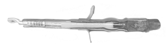
The created model was based on real heat-shrinkable termination (Fig.1 and Fig.2). The terminated cable is XRUHAKXS 120/50RMC 12/20 kV type of XLPE extruded MV cable [4].
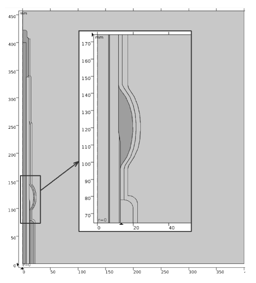
Fig.1. General view of examined cable termination
Fig.2. Part of sectioned modeled termination with visible semiconducting mastic (yellow) and semiconducting tube (black).
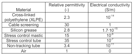
The cross-section of a real object allowed measuring the dimensions of each part of the accessory. Dimensions were measured with a caliper of 0.02 mm precision. Materials properties mentioned in [5]-[9] were used in the considered model.
Table I. Values of material properties used in model
.
Different cases of modeled cable termination were computed with the use of the AC/DC Module in the Comsol Multiphysics environment. Figure 3. shows a general view of the axisymmetric model of correctly assembled heatshrinkable MV cable termination and magnified part with a cutting point of cable screening covered by stress control mass.
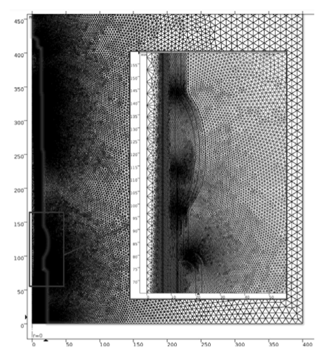
To fulfill the requirements of the FEM algorithm some boundary conditions should be applied. In both, electrostatic and AC analysis, Dirichlet boundary conditions were chosen, which means selected conductors surfaces obtain electric potentials. The next step for any solved problem is to build the mesh. Discretization (Fig.4.) of examined areas was made by automatic built-in algorithm with manually slightly changed parameters like the ratio between the size of two adjacent grid elements to dense mesh in important areas with expected electric field intensification.
To solve partial differential equations MUMPS (MUltifrontal Massively Parallel Sparse direct Solver) direct solver was used.
Fig.3. Axisymmetric model of heat-shrinkable cable termination with magnified cable screen cutting point area
Fig.4. Discretization of considered cable termination with magnified cable screen cutting point area
IV. Results of simulation
Correctly assembled cable termination
This section aims to investigate the electric field distribution of clean and properly assembled termination and compare results of simulation on the same model but under two different physics mentioned in section II.
Fig.5. Potential distribution as a result of a) electrostatic and b) AC analysis for correctly assembled cable termination
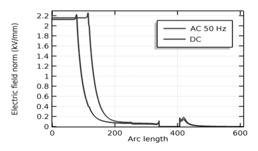
The first results of electric field simulation for both possibilities show (Fig.5) substantial difference in its distribution. Area of discontinuity of uniformity of electric field has moved from cable screen ending closer to cable semiconducting screen layer ends. Graph (Fig.6) present electric field strength for both possible simulation types along the straight line in cable termination at radius r = 11 (mm), where the green line is for electrostatic analysis and the blue one is for AC analysis.
Fig.6. Electric field strength inside cable termination at radius 11(mm) from the axis in properly assembled object
Cable termination without semiconducting mastic
This section consist investigation of electric field distribution of termination assembled with omission of semiconducting mastic and compare results of “electrostatics” and “electric current” simulation on the same model (section II).
Fig.7. Potential distribution as a result of a) electrostatic and b) AC analysis for incorrectly assembled cable termination (without semiconducting mastic).
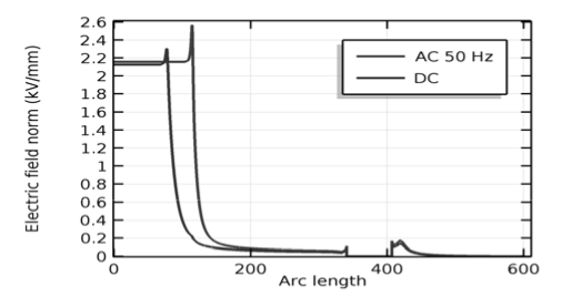
As in the first case also two quantities distribution was considered: potential distribution (Fig.7) on the surface of the cross-sectional area of termination and part of its surrounding, and electric field strength (Fig.8) longwise line on radius r = 11(mm) from the axis of a 2d-axisymmetric model of cable termination.
Fig.8. Electric field strength inside cable termination without mastic at radius 11(mm) from the axis.
Cable termination without semiconducting mastic and stress control tube
This section aims to investigate the electric field distribution of improperly assembled termination and compare results of simulation on the same model but under two different types of physics (section II).
Moreover, maximal electric field potential value from AC simulation as before is higher than in electrostatic solution.
Once more electric field distribution significantly changes (Fig. 9) only because of use different type of simulation conditions. Both analyzed quantities: potential (Fig.5, 9) and electric field strength (Fig. 6, 10) show that difference.
Fig.9. Potential distribution as a result of a) electrostatic and b) AC analysis for incorrectly assembled cable termination (without semiconducting mastic and stress control tube).
Fig.10. Electric field strength inside cable termination without semiconducting mastic and tube at radius 11mm from the axis.
V. Conclusions
That means the results of modeling could affect the design of a final product and its reliability and also position on the market. As it has been shown in the previous part of the article, incorrect choice of physics type could easily lead to erroneous conclusions. The possibility of an incorrect assembly of cable accessory constrain the designer to change the project and also the production process, therefore, it is very important to carefully build a numerical model with the correct parameters and correctly chosen physics. The best way to obtain it is to set model parameters possibly closest to the designed work conditions of the real object.
In the case of cable termination, it is very risky to simulate it with the electrostatic field. Regardless of modeled mistakes in the assembly process, this study shows that for electrostatics the most electrically stressed area appears always at the end of the deflected cable screen.
The omission of semiconducting termination parts assembly lead to an increase of potential gradients close to cable screen end.
REFERENCES
[1] Gulski, “Knowledge rules for partial discharge diagnosis in service”, Cigre TF 15.11/33.03.02, 2002, pp. 1-88. [2] K.P. Meena, B.N. Rao, T. Thirumurthy, G.K. Raja, “Failure analysis of medium voltage cable accessories during qualification tests”, 10th IEEE Int. Conf. Properties and Applications of Dielectric Materials, Bangalore, India, 2012, pp. 1-4 [3] G. Mazzanti; M. Marzinotto, “Combination of probabilistic electro-thermal life model and discrete enlargement law for power cable accessories”, 2016 IEEE International Conference on Dielectrics (ICD), vol.2, 2016, pp.780-783 [4] NKT Cables, XRUHAKXS 12/20 kV Data Sheet, 2016 [5] Aarnio, Anssi, “Characterization of non-metallic materials for medium voltage, cable accessories”, Master’s thesis, Tampere University of Technology, Material Science, 2010 [6] “SCO Silicone Grease Compound”, Electrolube company catalogue, Revision: 3 April 2016 [7] Illias, H. A.; Lee, Z. H.; Bakar, A. H. A. & Mokhlis, H. 2012. Distribution of electric field in medium voltage cable joint geometry. 2012 IEEE International Conference on Condition Monitoring and Diagnosis 23–27 September 2012, Bali, Indonesia. [8] Olli Kuusisto, “The Effects of Installation-Based Defects in Medium Voltage Cable Joints”, Bachelor thesis, Helsinki Metropolia University of Applied Sciences, Electrical Power Engineering, 2016 [9] I.A. Metwally, A.H. Al-Badi, A.S. Al-Hinai, F. Al Kamali and H. Al-Ghaithi, “Influence of Design Parameters and Defects on Electric Field Distributions inside MV Cable Joints”, IEEE 2016, Proceedings of the 18th Mediterranean Electrotechnical Conference (MELECON) [10] Ciuba M., Owsiński M., Sul P.: Analiza rozkładu pola elektrycznego w termokurczliwej głowicy kablowej z wadą montażu, in: Elektronika – konstrukcje, technologie, zastosowania, vol. 1, no. 11/2016, 2016, pp. 64-66, DOI:10.15199/13.2016.11.13 [11] M. Borecki, J. Starzyński, Z. Krawczyk, “The comparative analysis of selected overvoltage protection measures for medium voltage overhead lines with covered conductors”, Conference on Progress in Applied Electrical Engineering, ISSN 978-1-5386-1528-7, pp. 1-4, 2017, DOI: 10.1109/PAEE.2017.8009014 [12] M. Borecki, S. Wincenciak, “Simulation of Electric Field on the Surface of a Long Flashover Arrester”, 17th International Conference on Computational Problems of Electrical Engineering (CPEE 2016), ISSN 978-1-5090-2800-9, pp. 1-4, 2016, DOI: 10.1109/CPEE.2016.7738763
Authors: Maciej Ciuba1, Michał Wojciechowski1 , Maciej Owsiński2 , Michał Borecki1, Warsaw University of Technology (1), Koszykowa 75, 00-662 Warszawa, Poland e-mail: maciej.ciuba@ee.pw.edu.pl, michal.wojciechowski@ee.pw.edu.pl Institute of Power Engineering – Research Institute (2), Mory 8, 01- 330 Warszawa, Poland e-mail: maciej.owsinski@ien.com.pl
Source & Publisher Item Identifier: PRZEGLĄD ELEKTROTECHNICZNY, ISSN 0033-2097, R. 96 NR 4/2020. doi:10.15199/48.2020.04.25
Published by Juliya MALOGULKO, Svyatoslav VYSHNEVSKY , Iryna KOTYLKO, Natalia SOBCHUK, Vinnitsa National Technical University
Abstract. The article analyzes the pace of increase in the generation of photovoltaic stations in the context of the combined electricity system of Ukraine and the energy supply company of PJSC “Vinnytsyaoblenergo”. An analysis of existing regulatory documents regulating the work of photovoltaic stations has been carried out. Within the framework of the considered documents, the criteria for assessing the reliability of the operation of electric networks, namely, the length of long breaks in electric power supply of consumers of electric energy SAIDI are defined. The interconnection of the change of reliability indices of electric networks operation with the increase in the number and installed capacity of renewable energy sources, in particular photovoltaic stations (PV), is shown. In order to increase the reliability of power supply, a method of its renewal has been proposed, due to the joint use of generation of small hydroelectric power stations and PV stations.
Streszczenie. W artykule analizowano kombinowany system energetyczny na Ukrainie zawierający ogniwa fotowoltaiczne. Na podstawie dokumentacji analizowano niezawodność systemu biorąc pod uwagę przerswy w dostawie energii. Zaproponowano poprawę przez dołączenie małych elektrowni wodnych. Wpływ rozproszonych źródeł energii na niezawodność sieci elektrycznej
Keywords: dispersed energy sources, photovoltaic stations, local electric systems, small hydroelectric power stations. Słowa kluczowe: rozproszone źródła energii, ogniwa fotowoltaiczne, niezawodność
Introduction
In 2015, our state was one of the first to ratify the Paris Climate Agreements, thus confirming its intentions and commitments to integrate into the EU energy system and carry out energy reforms in the framework of the requirements of the Third Energy Package, which includes, among other things, the creation of favorable conditions for the introduction of new energy generating capacities renewable energy sources (RES).
The National Renewable Energy Action Plan for the period up to 2020 stipulates that the share of renewable energy generation in final energy consumption should reach 11% [1].
Nowadays, Ukraine demonstrates the highest pace of signing agreements for future accession of RES, but it poses great risks to the outdated energy network [2]. The key is that, according to official information of SRFEU, in I quarter. In 2018, 159.4 MW were put into operation, generating capacities – 54 objects of the electric power industry (2.4 times exceeding the capacity put into operation for the same period in 2017). At the same time, the objects of wind electric station (WES) and photovoltaic (PV) make up 92% of the installed capacities, and the average unit capacity of the electric energy objects introduced at that time is 3 MW. The installed capacity of WES and PV in Ukraine as of mid-2018 is 1353 MW (512 and 841 MW respectively), which has almost no effect on the balance of power. Their deviations from the planned generation are offset by maneuvering power.
In 2017, the number of technical specifications and contracts signed with Ukrenergo for joining high-voltage networks of green energy facilities, compared with 2016, increased by more than 30 times the power indicator. This is a crazy pace and this tendency persists.
According to Ukrenergo, contracts for joining by 2025 to networks of green energy installations with a capacity of 7426 MW (WES – 4200 MW, and PV – 3226 MW, excluding large hydroelectric power stations) have already been signed. However, the united energy system (UES) can only accept up to 3,000 MW of solar and wind power plants without the risk of unbalance and serious changes in its structure.
The system operator in his research stresses that PV and WES in terms of stability [3-6] of electricity supply are unreliable. Deviations from scheduled charts over the course of the day amount to more than 450 MW at a set power of 1217 MW. One more specific feature of the installation of renewable energy sources is their uneven distribution throughout Ukraine. Thus, the presence of one powerful source of up to 3 MW or several less powerful ones up to 0.5 MW connected to one substation of the distribution electric network (DEN), makes it possible to consider DEN as a local electrical system (LES). And for the local electrical system, there are not yet clear legislative acts that will require the operation of renewable energy sources.
Particularly acute for distributive electrical networks is the question of reliability and uninterrupted power supply. According to the Resolution of the National Commission for State Regulation in the Fields of Energy and Utilities (SRFEU) dated June 12, 2018 “On Approving the Procedure for Ensuring Quality Standards for Electricity Supply and Providing Compensation to Consumers for Failure”, [7] determined indicative, qualitatively characterizing the level of reliability of work DEN But, taking into account the pace of increasing the generation capacity of RES, in particular PV, it is expedient to carry out an analysis of changes in the determined indicators in terms of its growth.
Aim of the research – The purpose of the article is to assess the influence of photovoltaic generation on the reliability of the operation of electric networks and develop a method for its improvement.
Main materials of the research
In accordance with the IEEE 1366-2012 [8] and the SRFEU Resolution “On Approval of the Targets of Reliability (Continuity) Electricity Supply for 2018” [9], the main indicators of the reliability of operation of electric networks, including those with renewable energy sources, are quantified and qualitative breaks in electricity supply.
Classification of interruptions in electrical supply according to DSTU EN 50160: 2014:
a) scheduled, when the consumer is informed in advance about them;
b) Emergencies caused by long-term or short-term short circuits that are most often the result of external events, equipment failure or third-party interference in its operation Random breaks are classified as:
1) long interruptions (longer than three minutes); 2) short-term interruptions (including up to three minutes).
– System Average Interruption Duration Index
.
Where ri – the time of restoration of electricity, Ni – the number of breaks in the electricity supply of consumers in the reporting period, NT – the total number of consumers in the electrical network.
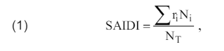
Increasing the share of generating renewable energy sources, for example, only those with the largest increase in power, namely wind and photovoltaic stations, are analyzed (Fig. 1).
At the beginning of 2015, the total installed capacity of the PV was 315 MW. Over the past four years, their capacity has increased more than 3 times and at the end of 2018 – 1100 MW. It should be noted that the PV are unevenly located on the territory of Ukraine, and in their turn, it is quite difficult to assess their impact on the reliability of electricity supply networks.
Fig.1. Dynamics of power generation of renewable energy sources in the UES of Ukraine. The total installed capacity of wind power stations in UES, 1 – wind electric station, 2 – photovoltaic stations, 3 – total renewable energy sources.
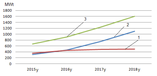
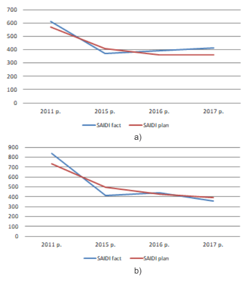
In fig. 2 shows the SAIDI change for 2011, 2015-2018, the average for the UES for urban and rural electric networks.
Fig.2. Change of target indicator SAIDI (red curve) and actual (blue curve) for (a) urban electric networks; (b) rural electricity networks of the UES of Ukraine
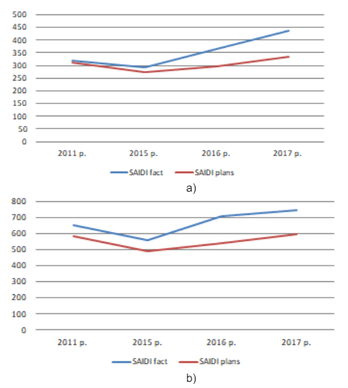
Based on statistical data, an increase in the generation capacity of renewable energy sources, the active introduction of which into electricity networks began to increase in 2015, may be the reason for prolonged electric power interruptions (SAIDI) electricity networks. The pace of increase in the generation of RES in the section of each power supply company is analyzed, among others Vinnytsyaoblenergo company has been allocated (Fig. 3), since here, starting from 2015, the growth of power generation capacity of the PV was the largest. Only the generation of PV is analyzed, because the wind potential for this region is insignificant. Consequently, the generation capacity in early 2015 was 41.3 MW and increased almost four times in the next three years – at the end of 2018, the power plant is 180 MW. However, the effect of the PV on the reliability of the networks here is significantly different from the impact on the network of the IEC as a whole (see Figure 4).
Fig.3. The pace of increase in the generation of PV in company ” Vinnytsyaoblenergo” (1) and the UES of Ukraine (2)
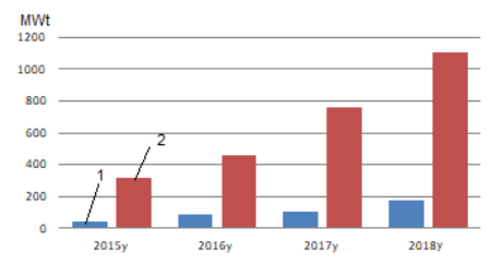
Simultaneous improvement of the level of technical equipment of the networks, as observed in Vinnytsyaoblenergo, together with the development of the PV, allows us to reveal their potential in view of the possibility of ensuring compliance with the indicator of the length of long interruptions in electricity supply in urban and rural electric networks (Fig. 4).
Fig.4. Change of target indicator SAIDI (red curve) and actual (blue curve) for a) city electric networks, b) rural electric networks of company “Vinnytsyaoblenergo”
The analysis of dependencies in Figures 2 and 4 allows us to conclude that it is possible to estimate and achieve the maximum effect from the implementation of renewable energy sources in view of the possibility of providing normative indicators of reliability (continuity) of electricity supply, taking into account the technical condition of the electricity network to which they are joining.
Thus, there is a whole range of tasks facing the industry experts to improve these indicators. Taking into account the rapid growth of electricity generation from distributed energy sources, it is expedient to use them jointly, in the context of a partial restoration of power supply to network demands. However, the use of such an approach is impossible without the coordination with relay protection systems and emergency automation of distribution networks 6-10kV. The connection of distributed generation objects to the DEN leads to a change in the main characteristics of the power system, on the basis of which the generally accepted concept of building relay protection (RP) was formed. At the level of the distribution network, multilateral power of the site of damage becomes possible, there are new, previously not typical types of disturbances and accidents, characteristics of electromagnetic and electromechanical transients are changing.
The problem of constructing RP significantly expands and complicates and, in the integrated approach, includes the solution of two groups of tasks:
– connected with the provision of the necessary technical perfection of RH of distribution electrical networks in which such stations are operated;
– associated with the creation of relay protection and automatics (RPA), which is installed at the point joining RES to the electrical network.
One of the ways to reduce the number and duration of failures in electricity supply is the possibility of joint use of different types of RES, namely, photovoltaic and small hydroelectric power stations in the tasks of partial recovery of consumers in the absence of electricity supply from centralized electricity supply networks. Another advantage of the joint use of such RES is to reduce the losses of the PV owners from the lack of electric power in the absence of tension on bus stations. These include the assurance of reliability of electric power supply to consumers maintenance of voltage levels within permissible limits, optimization of power flows in order to reduce losses, as well as maintenance of balance reliability in LES with combined electric supply from local and centralized sources of energy [11]. Determining the priority of solving problems arising in LES, note the balance reliability as the reliability of LES when its calculation model is determined by the balance of consumption and generation of electric energy, with the external supply being taken into account. The successful solution of other problems depends on the methods and means used to ensure the balance reliability. Technical and economic indices of LES depend on the balance of its active and reactive power [12]. The optimization of LES and EPS’s joint operation is considered in a number of research works [13]. Therefore, scheduling of the generation of photovoltaic stations is very important for maintenance of normal operating modes of the power system.
In the new economic conditions, photovoltaic power stations of direct transformation of energy are more and more widely used. Their use, in addition to making a profit from electricity sales, allows, under certain conditions, to unload the electricity networks and improve the quality of electricity [14].
Modeling Of Electrical Supply Restoration In Local Electrical Systems After Loss Of Centralized Power
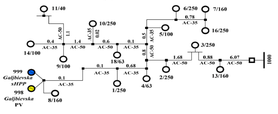
For the calculation of the regime parameters of the fragment of the scheme of the Yampil DEN, the source information about the Galzhbievska photovoltaic plant was analyzed:
– put into operation – 2013; – Installed power – 1381 kW; – Estimated annual generation – 1515 MWh; – type of Multi-Si modules.
Generation at this power plant takes place using SMA circular inverters, as well as multicrystalline silicon modules. This configuration ensures the optimal operation of the PV. The solar panels generate DC power, then through the inverters it enters 3 KTPs: KTP 0.4/10-630 kVA, 0.4/10- 1000kVA and 0.4 / 10-250 kVA.
The normal scheme of power output by the power plant implies that the electricity generated by the PV through the KTP of 0.4 / 10 – 630 kVA and 0.4 / 10 – 1000 by the line 27- 23 is supplied to the network connected to the substation Yampil 110 / 10kV. The model contains PV, consisting of 380 parallel connected strings of 15 photovoltaic modules per each type of panels – monocrystal (YL235P-29b). At the output of the inverter, a 0.4 / 10 kV transformer and a transformer 10 kV three-phase switch is installed. Another possibility of this model is that the generation of a photovoltaic station changes during simulation time, since the main parameters influencing the PV output, namely the level of solar insolation and the ambient temperature, therefore, the simulation of these parameters is presented in the form of a schedule that changes during the day.
The length of the feeder lines 15 of the 110/10 “Yampil” is 18 km. This feeder contains: 37 knots, 16 transformer substations, Galzhbievskaya PV and Galjbievska sHPP. Synchronous hydrogenerator with a power of 667 kVA, at the output of which is a voltage of 10 kV. The power network is represented in the form of four feeders and a centralized power source in the form of a 110/10 kV Yampil substation.
The total power of the transformer substations from which consumers feed is 2 149 kW. (Fig. 5), were considered.
Fig.5. Fragment of electric network where dispersed generation located
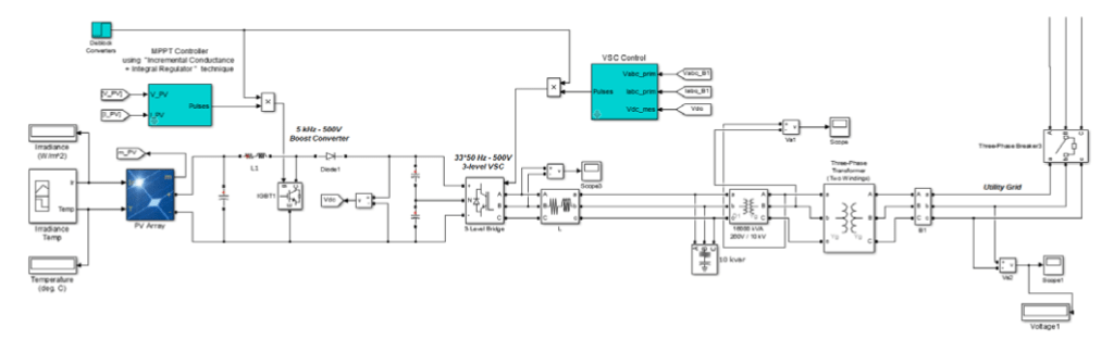
Fig.6. Simulink model of Galjbievska PV station which situated on the 998 bus
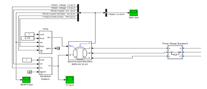
Fig. 7. Simulink model of Galjbievska small hydropowerplant which situated on the 999 bus
After analyzing the technical condition of the equipment of the electric networks, it was established that the most damaged element is the power lines. The computer model which showed in Figure 5, we divided for two computer mode (fig.6) – is a model of Galjbievska photovoltaic station and Figure 7 – is a model of small hydro power plant, which can supplying power to the photoelectric station bus. Due to the loss of centralized power supply from a centralized substation, consider two cases of restoration of electricity supply:
1. The combined use of a photoelectric and small hydroelectric power plant to restore consumers electricity supply.
2. Duration of the transition process, which will take place at the voltage supply to the PV bus from sHPP. In the framework of this work, the following modes of work are investigated and modeled:
1. The sinusoidal analysis of the voltage curve in paralleloperated photovoltaic and hydroelectric power plants at the power output of the common bus and in the absence of power supply from the 110 / 10kV Yampil 110 substation, it should be noted that the part of the load did not lose electricity due to the combined generation of the PV plant and sHPP (Fig. 8)
2. The next possible version of power supply for LES users, it is advisable to consider the mode of operation of the electrical grid, in which the running PV plant voltage is applied after the launch of a small hydroelectric power plant (Fig. 9).
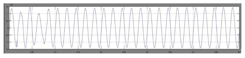
Fig.8. Changing the voltage curve as a result of the parallel operation of the PV plant and sHPP with the electric network
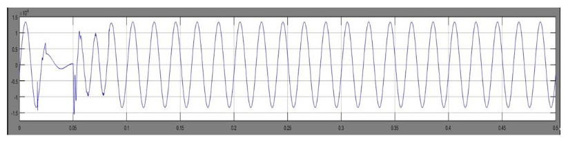
Fig.9. Changing the voltage curve as a result of voltage supply to the PV plant bus in sHPP
The results of simulation, on restoring the electricity supply of LES demands, by means of water drainage by a small hydroelectric power plant in order to supply voltage to the bus of a photovoltaic station, shows a slight distortion of the voltage curve.
The main idea of the work, is the implementation of mathematical modeling of the possibility of restoring the power supply of consumers of the electrical network that lost centralized power. Given the dependence of the photovoltaic power station’s operation on the electrical network, it can not function independently without supplying voltage. Proceeding from this, as a voltage source, hydroelectric power stations of low power are considered.
Conclusions
To increase the technical and economic efficiency of joint operation of distributed power sources and distribution electric networks, it is necessary to solve a number of tasks, which will allow to increase electricity generation of RES, reduce electricity losses in distribution electric networks, improve the quality and reliability of electricity supply to consumers.
In order to efficiently exploit distributed energy sources and their integrated use in power grids, especially in the sense of improving the reliability of power supply, it is necessary to develop a method for restoring consumer power supply, with the loss of centralized power supply. In the context of the transition from the wholesale electricity market of a single buyer to balancing and to electricity supply under bilateral agreements, in recent years and in perspective in Ukraine, there is a tendency of transition from purely centralized electricity to combined, when the number of local power sources is increasing. Moreover, the share of the latter in the energy balance of power systems is increasing. Local power sources, operating directly in the grids of 10-6-0.38 kV, include both traditional sources of low power and alternatives.
The results of simulation of the possibility of restoring electricity supply to LES users in the event of a loss of centralized power show high potential for the use of RES in this direction. In particular, RES may be a significant time to maintain the power of consumers while ensuring a standard for the quality of electric energy and the cost- effectiveness of the operation of electricity grids
REFERENCES
[1] Derzhavna tsilʹova ekonomichna prohrama enerhoefektyvnosti i rozvytku sfery vyrobnytstva enerhonosiyiv z vidnovlyuvanykh dzherel enerhiyi ta alʹternatyvnykh vydiv palyva na 2010-2020 roky// Zatverdzhena postanovoyu Kabinetu Ministriv Ukrayiny vid 01.03.2010 r. № 243 [Elektronnyy resurs] // Rezhym dostupu: http://zakon2.rada.gov.ua/laws/show/243-2010-%D0%BF [2] Zvit pro rezulʹtaty diyalʹnosti u 2017 rotsi [Elektronnyy resurs] // Zatverdzheno postanovoyu SRFEU vid 23 bereznya 2018 roku № 360. Rezhym dostupu do resursu – URL: http://www.nerc.gov.ua/data/filearch/Catalog3/Richnyi_zvit_SRFEU_2017.pdf [3] Lezhniuk P. D. Otsinyuvannya vplyvu na yakistʹ funktsionuvannya lokalʹnoyi elektrychnoyi systemy vidnovlyuvanykh dzherel elektroenerhiyi / P. D. Lezhniuk, V. O. Komar, D. S. Sobchuk // Visnyk Kharkivsʹkoho natsionalʹnoho tekhnichnoho universytetu silʹsʹkoho hospodarstva imeni Petra Vasylenka. Problemy enerhozabespechennya ta enerhozberezhennya APK Ukrayiny. – Kharkiv : KHNTUS·H, 2013.Vypusk 141. S. 8–10. [4] Kulyk V. V. Optymalʹne keruvannya rozoseredzhenymy dzherelamy elektroenerhiyi z asynkhronnymy heneratoramy zasobamy Smart Grid [Elektronnyy resurs] / V. V. Kulyk, T. YE. Mahas, YU. V. Malohulko // Naukovi pratsi VNTU. – 2011. – №4.– S. 1–6. – Rezhym dostupu do resursu : http://praci.vntu.edu.ua/article/view/1404/999. [5] Kyrylenko O. V. Power Engineering of Sustainable Development: Challenges and Construction Paths / O. V. Kirilenko, AV Prachevnik // Proceedings of the Institute of Electrodynamics of the National Academy of Sciences of Ukraine. Special issue. 2010. 10-16. [6] Kyrylenko O. V. Tekhnichni aspekty vprovadzhennya dzherel rozpodilenoyi heneratsiyi v elektrychnykh merezhakh / O. V. Kyrylenko, V. V. Pavlovsʹkyy, L. M. Lukʺyanenko // Tekhnichna elektrodynamika. 2011. № 1. S. 46–53. [7] Pro zatverdzhennya Poryadku zabezpechennya standartiv yakosti elektropostachannya ta nadannya kompensatsiy spozhyvacham za yikh nedotrymannya// Zatverdzhena postanovoyu Kabinetu Ministriv Ukrayiny vid 12.06.2018 r. № 375 [Elektronnyy resurs] // Rezhym dostupu: http://zakon.rada.gov.ua/laws/show/v0375874-18 [8] IEEE Guide for Electric Power Distribution Reliability Indices,” in IEEE Std 1366-2012 (Revision of IEEE Std 1366-2003) , vol., no., pp.1-43, 31 May 2012 doi: 10.1109/IEEESTD.2012.6209381 [9] Pro zatverdzhennya tsilʹovykh pokaznykiv nadiynosti (bezperervnosti) elektropostachannya na 2018 rik // Zatverdzhena postanovoyu Kabinetu Ministriv Ukrayiny vid 14.06.2018 r. № 392 [Elektronnyy resurs] // Rezhym dostupu: http://www.nerc.gov.ua/index.php?id=32667 [10] Lezhnyuk P.D. Vozobnovlyayemyye istochniki energii v raspredelitel’nykh elektricheskikh setyakh: Monografiya / P.D. Lezhnyuk., A.A. Koval’chuk, A.V. Nikitorovich, V.V. Kulik. – Vinnitsa, 2014. – 204 s. [11] Q. Jiang, G. Geng, C. Guo, and Y. Cao, “An efficient implementation of automatic differentiation in interior point optimal power flow,” IEEE Trans. Power Syst., vol. 25, no. 1, pp. 147–155, Feb. 2010. [12] Kulyk V.V. Operational control of the flow of reactive power in the distribution of electrical dispersed generation // Proceedings of the Institute of Electrodynamics National Academy of Sciences. Collected Works. Special-start you. – 2013. – P. 151-158. [13] Seyed Mohammad Hossein Nabavi, Somayeh Hajforoosh, Mohammad A.S. Masoum, “Placement and Sizing of Distributed Generation Units for Congestion Management and Improvement of Voltage Profile using Particle Swarm Optimization”, IEEE Transactions on Power Systems, 2011. [14] C. L. T. Borges and D. M. Falcao, “Optimal distributed generation allocation for reliability, losses, and voltage improvement”, Int. J. Elect Power Energy Syst., vol. 28, no. 6, pp. 413–420, Jul. 2006.
Published by Jan NEDOMA, Marcel FAJKUS, Radek MARTINEK, VSB – Technical university of Ostrava
Abstract. This article deals with the measurement of electric current in the energy via optical fibers. Nowadays, the measurement of the electrical current by using optical fiber most commonly based on the principle of Faraday effects, thus the magneto-optic effect. FOCS (Fiber-Optic Current Sensor) is very accurate, modular and easy to install. Another advantage is the isolation of the measuring part from the primary technology, which is sensed. Optical fibers can also be used to measure the inside of the transformer. It also offers the possibility of measuring the temperature of winding. The main contribution of the paper is to summarize interesting published results to date, approaches and basic principles leading to the analysis and to defining the electrical values such as electrical current using fiber optic technology.
Streszczenie. W artykule opisano możliwości pomiaru prądu przy wykorzystaniu światłowodów. Czujnik FOCS (fiber optic current sensor) jest dokładny I łatwy do instalacji. Inną zaletą jest oddzielenie galwaniczne od toru prądowego. W artkule przedstawiono przegląd prac na ten temat, przegląd rozwiązań konstrukcyjnych I zastosowań oraz analizę właściwości metody. Pomiar pradu elektrycznego przy wykorzystaniu światłowodów.
Keywords: fiber-optic technology, electrical current, current sensor, magneto-optic effect. Słowa kluczowe: światłowody, pomiar prądu, zjawisko Faradaya.
Introduction
The fiber-optic sensor is based on the use of Faraday’s magneto-optical effect (year of discovery is 1845), in which there is a magnetic rotation of plain of the polarized light, see Figure 1. However, the use of this phenomenon for the measurement of electrical quantities has only occurred thanks to the development of fiber optic technology. The rate of twisting of the polarization plane is directly proportional to the path d, after which the light in the given environment spreads and size of the components of the vector of magnetic induction B in the direction of light propagation. The orientation of the vector determines the meaning of the polarization plane. The size of the angle of rotation β, by which the polarization plane is rotated (see Fig. 1) can easily be calculated by a simple relationship (1):
(1) β = V * B * d,
where: V – Verdet constant, B – density of magnetic induction, d – length of path The Verdet constant depends on the wavelength of the light and it is an optical “constant” that describes the strength of the Faraday-effect for a particular material.
Fig.1. Basic scheme of the Faraday-effect.
Fiber-optic current sensors are referred to as FOCS (Fiber-Optic Current Sensor). Figure 2 shows the principle of the fiber-optic current sensor FOCS. FOCS benefits are high accuracy, high bandwidth: detection of current ripple and transients, wide temperature range, full digital processing, uni- or bi-directional current measurement, analogue and digital outputs, easy to install, adaptable shape of sensing head, small size and weight, no magnetic centering necessary, no magnetic overload problem, immunity to electromagnetic interference and many others.
Fig.2. Principle of the fiber-optic current sensor FOCS
An important application area of FOCS is the metallurgical industry, where an electrolytic process is used to obtain precious metals. Typical electrolyzers work with DC (Direct Current) in the order of several hundred thousand amperes (up to 500 kA). Fiber-optic sensors can be used as measuring transducers and provide a number of benefits, such as easier installation, smaller dimensions and high accuracy of measurement. Nowadays, the target application area for the use of the fiber optic FOCS sensors is to measure, control and protect the substations. Also, the advantage is that due to small dimensions and weight, FOCS can be integrated into an existing device, such as switches and bushings. The application is also in the DC lines of very high voltage (HVDC) used for the transmission of electricity over long distances. From the point of view of the security function of the protection there is a significant advantage that even in the case of high short-circuit currents, there is no overloading and distortion of the output signal, which we encounter with conventional current transformers. Another advantage is the isolation of the measuring part from the primary technology, which is sensed [1-6].
The main contribution of the paper is to summarize interesting published results to date, approaches and basic principles leading to the analysis and to defining the electrical values such as electrical current using fiber optic technology.
Approaches and results
An advanced fiber-optic current sensor is based on the recirculating architecture of fiber loop for significantly enhancing the current sensitivity. The recirculating loop is created by a 2×2 optical switch and the single mode fiber is used as the sensing head, see Fig. 3. Authors experimentally obtained a sensitivity of 11.5 degrees/A for1000 meters fiber and a sensitivity of 21.2 degrees/A for 500-meters fiber [7].
Fig.3. Basic scheme of Sagnac fiber optic current sensor
A smaller fiber sensing coil is required in order to that the FOCS meet the needs of the high voltage watt-hour meter for measuring smaller current with the better performance. The FOCS sensing coils (<10 cm in diameter) is achieved by the special spun highly birefringent fiber. The ability to resist bending is analyzed in the comparison between the fiber sensing coils by the special spun highly birefringent fiber and the fiber sensing coils by the low birefringent fiber. The measurement error of the FOCS is ± 0.2 % from -40 °C to 70 °C under considering temperature compensation, and the FOCS shows the excellent performance of temperature characteristics, linearity and accuracy in a current range from 1 A to 120 A [8].
Next article studies the using an FOCS for the measurement of plasma current in the fusion reactor (ITER). The sensor is based on a classical FOCS interrogator involving the measurement of the state of polarization rotation when the light in presence of a magnetic field (Faraday effect) in an optical fiber surrounding the current and terminated by a Faraday mirror. The objective of the simulations is to quantify the ratio (beat length over the spun period of the spun fiber) enabling a measurement error in agreement with the ITER specifications. The simulation work showed that a L-B/S-P ratio is 19.2 [9].
The paper [10] researched on the error ratio of FOCS induced by temperature drift. The reason of FOCS error drift was described to explain the relationship among temperature, linear birefringence and error of FOCS ratio. In the range of testing temperature, both the ratio error of FOCS and linear birefringence had a linear relationship with temperature. The FOCS ratio error had a linear relationship with experiment temperature similar to 60 °C.
Complex transforming processes of polarization state induce illegal linear polarization state and illegal circular polarization state in Sagnac fiber-optic current sensor, which, decrease the performance of S-FOCS. Based on polarization state error models of Sagnac fiber-optic current sensor, authors made experiments to evaluate performances of several key components, including polarizer, quarter-wave retarder and sensing head, then, investigate the influence of several main polarization error factors on S-FOCS’s performance. The result shows that the changing degree of polarization state causes bias instability, nonlinear of scale ratio, and random noises of SFOCS, and influents S-FOCS’s performance [11].
Paper [12] describes the structure and principle of the FOCS created by Faraday mirror. The performance of the FOCSs is limited by the linear birefringence (LB). Faraday mirror can be employed to compensate the LB using the non-reciprocity of Faraday effect and the reciprocity of LB. The results indicate if that the influence of LB disappears then the current is null. However, if the current is not zero, the LB is not removed and the effect extent is different for different LB. The Faraday rotation can be deduced from the detected signals and the LB need not be compensated physically by employing this technique.
A special spun linear birefringent fiber was designed and created for FOCS based on polarization-rotated reflection interferometers. In contrast with conventional sensing fibers used in FOCS, the fiber uses a function of a quarter wave plate. The output of sensor has a good linearity performance in a wide range of current (10 to 5000 A/rms). The ratio error is ± 0.1 % and the phase error is ± 2 min at AC current of 1000 A [13].
Article [14] investigate the design principle exploiting the geometric rotation effect for the sensing coil of the fiberoptic current sensor (FOCS) on the basis of the polarization-rotated reflection interferometer. The sensing coil is formed by winding the low birefringence single-mode optical fiber in a toroidal spiral. If the rated current is 1200 A/rms, the sensing coil can ensure the scale factor error of the sensor of 0.2 S over a temperature range from -40 °C to 60 °C.
A prototype fiber-optic current sensor (FOCS) created by Sagnac interferometer is designed and tested for monitoring current up to 4000 A. Sensor is tested for nominal current 1 A up to 800 A. The output of sensor has nonlinearity of ± 0.5 % [15].
A highly accurate fiber-optic current sensor for AC and DC up to 100 kA was investigated. Reciprocal optical circuit and method of signal processing based on the relationship of modulation and demodulation of this sensor were analyzed. The sensor achieved accuracy to within ± 0.2 % at -40 °C to 80 °C with inherent temperature compensation, resolving power for small AC current was less than 0.5 A, angle difference was less than ± 2 min [16].
Authors [17] propose a new technique to reduce the bending-induced linear birefringence (LB) by fiber polarization rotator (FPR) in the reflective fiber-optic current sensor (FOCS), see Fig. 4. A comparison was made between the proposed FPR scheme and the conventional scheme on measurement errors. Simulation shows that the proposed scheme has a large improvement on such LB reduction by an order of magnitude.
Fig.4. Basic scheme of FOCS without FPR.
A new method for measurements of lightning on wind turbines by fiber-optic current sensors (FOCS) was developed. FOCS are resistive with respect to electromagnetic interference (EMI), because the magnetic field produced by the current of lightning is directly converted into an optical signal in this device. The sensor cannot be damaged by over-current coming from an unexpected surge caused by a lightning. However, the accuracy of current measurements with FOCS is affected by the environmental perturbations, such as mechanical vibration and temperature changes [18].
A fiber-optic current sensor employs phase shifting algorithms to process the optical signal is described. Here, the sensing element consists of a coil low birefringence fiber which placed between one polarizer and four analyzers. In the polarimeter, the output light from the sensing element of current is divided into 4 beams through 3 non-polarizing beam splitters, and an analyzer and a detector are placed in each beam path. The design of the sensor, results and shift algorithms will be presented [19].
Authors presented fiber-optic current sensor for DC up to 500 kA. The sensor offers significant advantages with regard to performance and ease of installation compared to state-of-the-art Hall-effect-based current transducers. The sensor exploits the Faraday effect in an optical fiber and measures the path integral of the magnetic field along a closed loop around the current-carrying bus bars. The differential magneto-optic phase shift of left and right circular light waves propagating in the fiber is detected by a polarization-rotated reflection interferometer. The sensor achieves accuracy ± 0.1 % over a wide range of currents and temperatures [20].
Next paper presents a fiber-optic current sensor (FOCS), customized for measurement of harmonic current in high-voltage electric power systems. The practical application of this device has been verified experimentally at a thermal power plant. The measurements have been made for the operation of a 6kV induction motor with different load conditions and the thyristor excitation of a 15 kV AC generator [21].
A fiber-optic current sensor (FOCS) created by the Faraday effect is presented. The sensor of current is realized using the all-fiber low-coherent reflection interferometer. An Erbium-doped fiber, a super-fluorescent radiation source, and a sensing spun high-birefringence fiber coil are applied in the interferometer. The sensitivity of the sensor is about 70 mA/root Hz, the scale factor error is about 0.5 %, the range of measured currents is 0.1 A~3000 A, and the bandwidth is up to 10 kHz [22].
Authors [23] present FOCS based on Faraday effects with the magnetic concentrator. According to the measured values of AC up to 1 kA, a calibration procedure was performed. A well-known temperature dependence of the Faraday current sensor and its influence on the measurement accuracy are tested using a special doublelayer thermal insulated chamber.
A fiber-optic current sensor (FOCS) based on a Sagnac interferometer is presented to measure high-voltage AC current in electric power systems from 5 A to 3200 A, see Fig. 5. A simple analytical expression for the sensor has been derived, the input-output performance and the temperature dependence of FOCS have been experimentally investigated. The simple geometry of sensor gives high accuracy and sensitivity, wide dynamic range, and immunity to slow-variance temperature and other environmental fluctuations [24].
Fig.5. Basic scheme of FOCS using Differentiating Sagnac Interferometer.
Next, it is discussed a new configuration of FOCS which increases the linearity range of the device without decreasing its sensitivity. In this way, the whole system behaves as a ”null-detector”. However, the effect of bending-induced linear birefringence is taken into account in the design and optimization of the sensor. It is shown that the response of the experimental apparatus is temperature independent and that its bandwidth gets values higher than 1 MHz [25].
Fiber-optic current sensor based on the Faraday effect of magneto-optic materials, in the isotropic optical transparent medium, and the magnetic field can make the plane polarized light propagating polarization plane rotated along the magnetic field. By mathematical optimization method, paper [26] discusses the end fitting, the average points fitting, least square method, and the optimal linear least absolute deviation method which is applicated to the linear characteristics of the fiber-optic current sensor. The results show that different linear fitting methods have different results. Using the least square method and best linear fitting method (regression line) obtained FOCS’s linearity fitting degree is ± 0.069 % and ± 0.071 % respectively.
The error drift caused temperature shift reduces the accuracy of FOCT. Using two models, authors quantitatively researched the error ratio drift, and obtained temperature characteristics of FOCT: within the tested range of temperature (10~60 °C), both the FOCT ratio error and linear birefringence phase difference changes linearly with temperature [27].
The residual linear birefringent of sensing fiber, temperature and vibration sensitivity severely influence the accuracy of Sagnac fiber-optic current sensor. A sensing fiber can be used in FOCS with spun high-birefringent fiber. This S Hi-Bi fiber includes three sections: two terminal sections with variable spin-rate along fiber were utilized to substitute the fiber quarter-wave plates, respectively converting the light polarization state from the linear one to the circle one, and vice versa; and the middle section with a uniform spin-rate was utilized as the current sensing fiber which maintains the circular state polarization and compresses the residual linear birefringent during the light propagation [28].
The fiber-optic current sensors utilize the effects of magnetic-field imposed on the change of polarization state of light in the fibers. This sensor has a lot of advantages over conventional current sensors, see Fig. 6. To eliminate the vibration sensitivity, an improved light path of the reflective fiber-optic current sensor is proposed, which makes the discharge of Sagnac effect with Sagnac effect itself and do not disturb Faraday effects [29].
Fig.6. Basic scheme of a novel fiber-optic current sensor.
To improve the performance, a fiber-optic current sensor was presented and using Jones matrix, its polarization error was studied. By establishing the Jones matrix expression of the main optical devices, an interference expression of this sensor was introduced and the influence of imperfection of optical devices on the measurement accuracy was analyzed [30].
High-precision methods and devices are one of the most important modern engineering development lines in optimal energy consumption sphere. However, there are a few small-sized instruments which allow conducting precision measurements without breaking the circuit. Paper [31] presents information about conducted Faraday Effect research and general construction of the simple fiber-optic current sensor (FOCS).
In 2005, ABB introduced a high-performance fiber-optic current sensor for the measurement of DC up to 600 kA. Recently, ABB has developed the sensor further with a view to implementing it in high-voltage substations. It can be integrated into primary high-voltage equipment such as circuit breakers. By appropriately selecting the number of fiber loops, the measurement range can be optimized for specific applications [32].
According to the polarization coupling model of the polarization-maintaining delay fiber coil, considering the reciprocal parasitic waves with large amplitude, the interference intensity of the optical system in the fiber-optic current sensor (FOCS) is calculated, and the theoretical relationship between the scale factor and the polarization crosstalk of the delay fiber coil is obtained. The effect mechanism of the temperature dependence of the polarization crosstalk on the scale factor is revealed, and the corresponding suppression methods are proposed. The experimental results show that the temperature dependence of the FOCS can be improved greatly when lowering the tension of winding fiber, reducing the quantity of the glue, and utilizing the frame with low-temperature coefficient. The variation of the scale factor is decreased from 0.63 % to 0.07 % over the temperature range from -40 °C to 70 °C [33].
In Sagnac interferometer fiber-optic current sensor, errors from the residual linear birefringence and environmental temperature and vibration sensitivity severely influence the accuracy of this sensor. The spun highly linearly birefringent fiber was designed and the vibration insensitive Sagnac interferometer fiber-optic current sensor scheme was set up. In this scheme, the compensation fiber coil was designed to compensate the error caused by Sagnac effect in sensing fiber coil [34].
The fiber-optic current sensor was presented. According to a characteristic of interference signal, square wave modulation technique was applied to enhance the sensitivity of FOCS, and correlative demodulation scheme was proposed to show phase difference information. The sensor achieved accuracy within ± 0.25 % at -40~60 °C and the bandwidth exceeded 6 kHz [35].
ABB developed a new configuration of air-insulated switchgear (AIS) substations by using new circuit breaker (CB) technologies and optical sensors. The new disconnecting circuit breaker (DCB) ‘Combined’ placed inside the breaking chamber without any other components. The fiber-optic current sensors based on the Faraday effect is able to determine the current with a fiber-optic loop integrated with the conductors. FOCS also provide an interface with process-level devices for a substation automation system (SAS). The use of new DCB and optical sensors can improve the performance, efficiency, and reduce the footprint of a substation [36].
The nonlinearities of the response of an interferometric fiber-optic current sensor, which is associated with deviations of the light waves from perfect circular polarization, are investigated. The consequences of inherent temperature compensation of the Faraday effect using a non-90°-retarder are investigated for currents up to several 100 kA and temperatures between – 40 °C and 80 °C. The results are of particular interest to sensors for high DC in the electro-winning industry where measurement accuracy of ± 0.1 % is required up to 500 kA [37].
Fiber-optic current sensors (FOCS) based on Faraday magneto-optical effect have plenty of advantages in comparison to the traditional current sensors. However, the residual linear birefringence and environmental vibration sensitive problem are the fatal drawback in Sagnac fiberoptic current sensors. A vibration immunity sensing loop with a function of passive fiber-optic polarization control is proposed, which consist of a spun or twisted fiber with highly birefringence. A spun or twisted fiber possesses two crucial functions: Remove the residual linear birefringence and control polarization of light. It has been demonstrated that this FOCS has high sensitivity, considerable wide dynamic range, resistance to electromagnetic interference, and immunity of vibration [38].
Fig.7. Basic scheme of principle of S-FOCS.
The intrinsic birefringence of the sensing fiber is the main cause which affects the precision of measurement, and elimination of this cause is the key research topic. In paper [39] an interferometric fiber-optic current sensor configuration with a conjugate reflector is presented. The results show that the configuration with a conjugate reflector is more insensitive to linear birefringence than the configuration with an ordinary reflector. The residual linear birefringence of the sensing coil is about 6 times than that in ordinary mirror configuration for ± 0.2 % measuring accuracy.
Firms require highly accurate DC current sensors to control their processes and operations. FOCS has suitable performance and functionality and is smaller and lighter. Using the FOCS accuracy increased by 10 times, specified accuracy is maintained over a wide temperature range, and large bandwidth to enable rapid response to current ripple and transients. FOCS is also responsible for handling uni- and bi-directional DC to ± 500 kA with negligible power consumption [40].
ABB developed a sensor that represents a quantum leap in high DC measurements. This sensor offers outstanding precision and is smaller, lighter and much less complex than traditional transducers and it is about to change the future of high DC measurements. The new fiber-optic current sensor (FOCS) for high DC makes use of the Faraday effects [41].
The problem of polarimetric sensors is not discussed in this paper, but currently polarimetric sensors are also commonly used. Information on polarimetric sensors is available in articles published in the Electrical Review or in article [42].
Conclusion
This article is to summarize the interesting practical and theoretical published results to date, approaches and basic principles based on Faraday effect leading to the analysis and to defining the electrical values such as electrical current using the fiber-optic technology. Fiber-optic current sensor benefits are obvious and very useful for current applications The high accuracy, high bandwidth: detection of current ripple and transients, wide temperature range, no magnetic centering necessary, no magnetic overload problem, immunity to electromagnetic interference and many others.
Acknowledgements – This article was supported by the Technology Agency of the Czech Republic TA04021263 Project and by the Ministry of Education of the Czech Republic (Projects Nos. SP2017/128 and SP2017/79). This research was partially supported by the Ministry of Education, Youth and Sports of the Czech Republic through Grant Project no. CZ. 1.07/2.3.00/20.0217 within the framework of the Operation Programme Education for Competitiveness financed by the European Structural Funds and from the state budget of the Czech Republic. The Ministry of the Interior of the Czech Republic (Projects Nos. VI20152020008 and VI2VS/444) also provided support for this article. The Ministry of Industry and Trade of the Czech Republic (Project No. FV 10396) also provided support for this article.
References
[1] P. Siddons, N. C. Bell, Y. Cai, C. S. Adams, and I. G. Hughes, “A gigahertz-bandwidth atomic probe based on the slow-light Faraday effect,” Nat. Photonics, vol. 3, no. 4, 2009. [2] L. Weller, K. S. Kleinbach, M. A. Zentile, S. Knappe, I. G. Hughes, and C. S. Adams, “Optical isolator using an atomic vapor in the hyperfine paschen-back regime,” Opt. Lett., vol. 37, no. 16, 2012. [3] E. Prati, “Propagation in gyroelectromagnetic guiding systems,” J. Electromagn. Waves Appl., vol. 17, no. 8, 2003. [4] M. L. Kales, “Modes in wave guides containing ferrites,” J. Appl. Phys., vol. 24, no. 5, 1953. [5] S. Mancuso and S. R. Spangler, “Faraday rotation and models for the plasma structure of the solar corona,” Astrophys. J., vol. 539, no. 1 PART 1, 2000. [6] W. F. Magie, “Faraday’s Diary,” Science (80-. )., vol. 77, no. 1995, 1933. [7] J. Du, Y. Tao, Y. Liu, L. Ma, W. Zhang, and Z. He, “Highly sensitive and reconfigurable fiber optic current sensor by optical recirculating in a fiber loop,” Opt. Express, vol. 24, no. 16, 2016. [8] F. Yang, X. Hou, Y. Huang, and N. Peng, “Optical fiber current sensor with small size for the high voltage watt-hour meter,” in Proceedings of SPIE – The International Society for Optical Engineering, 2016, vol. 10158. [9] M. Wuilpart, B. Vanus, A. Andrasan, A. Gusarov, P. Moreau, and P. Mégret, “Study of a fibre optics current sensor for the measurement of plasma current in ITER,” in Proceedings of SPIE – The International Society for Optical Engineering, 2016, vol. 9916. [10] S. Cheng, Z. Guo, G. Zhang, W. Yu, Y. Shen, and S. Jin, “The analysis on temperature characteristic of fiber optic current sensor ratio error,” in Proceedings – 5th International Conference on Instrumentation and Measurement, Computer, Communication, and Control, IMCCC 2015, 2016. [11] L. Wang, M. Cao, Q. Liu, G. Wei, B. Li, and C. Lin, “Modeling and experimental verification of polarization errors in Sagnac fiber optic current sensor,” Optik (Stuttg)., vol. 126, no. 20, 2015. [12] R. Zhang, X. S. Yao, T. Liu, and L. Li, “The effect of linear birefringence on fiber optic current sensor based on Faraday mirror,” in Proceedings of SPIE – The International Society for Optical Engineering, 2014, vol. 9274. [13] P. Nai, S. Wang, and W. Tao, “A special spun birefringent fiber optic current sensor,” in Proceedings – 2013 12th International Conference on Optical Communications and Networks, ICOCN 2013, 2013. [14] C. Zhang, C. Li, X. Wang, L. Li, J. Yu, and X. Feng, “Design principle for sensing coil of fiber-optic current sensor based on geometric rotation effect,” Appl. Opt., vol. 51, no. 18, 2012. [15] A. Prakash et al., “Development of fiber optic current sensor for electric power industry application,” in 2012 International Conference on Fiber Optics and Photonics, PHOTONICS 2012, 2012. [16] C. Zhang, C. Wang, and S. Chen, “Theory and experimental research of a Y-phase-modulator based optical fiber current sensor,” in Proceedings of SPIE – The International Society for Optical Engineering, 2011, vol. 8199. [17] S. Zhou and X. Zhang, “Simulation of Linear Birefringence Reduction in Fiber-Optical Current Sensor,” IEEE Photonics Technol. Lett., vol. 19, no. 19, 2007. [18] S. G. M. Krämer, F. P. León, Y. N. M. Hernández, and B. Lewke, “Integration of a distributed fiber optic current sensor setup for lightning detection in wind turbines,” in Conference Record – IEEE Instrumentation and Measurement Technology Conference, 2007. [19] J. L. Flores, G. García-Torales, and V. H. Ortiz, “Optical current sensor using phase shift algorithms,” in Proceedings of SPIE – The International Society for Optical Engineering, 2007, vol. 6770. [20] K. Bohnert, H. Brändle, M. G. Brunzel, P. Gabus, and P. Guggenbach, “Highly accurate fiber-optic dc current sensor for the electrowinning industry,” IEEE Trans. Ind. Appl., vol. 43, no. 1, 2007. [21] S. J. Petricevic, Z. Stojkovic, and J. B. Radunovic, “Practical application of fiber-optic current sensor in power system harmonic measurement,” IEEE Trans. Instrum. Meas., vol. 55, no. 3, 2006. [22] V. P. Gubin et al., “All-fiber optical sensor of electrical current with a SPUN fiber sensing element,” in Proceedings of SPIE – The International Society for Optical Engineering, 2006, vol. 6251. [23] P. Mihailovic, S. Petricevic, Z. Stojkovic, and J. B. Radunovic, “Development of a portable fiber-optic current sensor for power systems monitoring,” IEEE Trans. Instrum. Meas., vol. 53, no. 1, 2004. [24] T. Wang, C. Luo, and S. Zheng, “A fiber-optic current sensor based on a differentiating Sagnac interferometer,” IEEE Trans. Instrum. Meas., vol. 50, no. 3, 2001. [25] A. Irace, G. Breglio, A. Luciano, L. Zeni, and A. Cutolo, “A novel configuration for a wide-range high-power fiber-optic current sensor,” Eur. Trans. Electr. Power, vol. 7, no. 5, 1997. [26] Z. Yue, W. Xiaofei, and M. Hao, “Study on the characteristics of all fibre optical current sensor linear fitting algorithm,” in 2015 IEEE 12th International Conference on Electronic Measurement and Instruments, ICEMI 2015, 2016, vol. 3. [27] S. Cheng, Z. Guo, G. Zhang, Y. Shen, P. Song, and H. Huang, “Temperature characteristic of fiber optic current sensor,” Gaodianya Jishu/High Volt. Eng., vol. 41, no. 11, 2015. [28] Y. Wang, M. Kang, L. Ren, and K. Ren, “Design of spun highbirefringent fiber for fiber optic current sensor,” Hongwai yu Jiguang Gongcheng/Infrared Laser Eng., vol. 44, no. 1, 2015. [29] S. Tao, F. Yue, L. Yipu, Z. Mengxue, D. Hailong, and W. Xinlao, “Simulation of polarization errors for all-fiber optic current sensors,” in Proceedings – 8th International Conference on Future Generation Communication and Networking, FGCN 2014, 2014. [31] P. Liu, K. Chen, S. Chen, and Z. Liu, “Study on polarization errors of re-entrant fiber-optic current sensor,” Bandaoti Guangdian/Semiconductor Optoelectron., vol. 35, no. 2, 2014. [31] M. G. Grigoriev and N. V. Turushev, Development of fiber optic current sensor, vol. 1040. 2014. [32] K. Bohnert, R. Thomas, and M. Mendik, “Light measures current: A fiber-optic current sensor integrated into a highvoltage circuit breaker | Strom messen mit Licht: Faseroptischer Stromsensor in einem HochspannungsLeistungsschalter,” ABB Rev., no. 1, 2014. [33] C. Li, C. Zhang, H. Sun, and H. Cui, “Effect of polarization crosstalk of polarization-maintaining delay optical fiber coil on the fiber-optic current sensor,” Zhongguo Jiguang/Chinese J. Lasers, vol. 41, no. 11, 2014. [34] Y. Wang, M. Kang, L. Ren, K. Ren, J. Xu, and N. Shi, “A novel compensation fiber coil for eliminating Sagnac Effect in fiber optic current sensor,” in Chinese Control Conference, CCC, 2013. [35] C.-Y. Zhang, C.-X. Zhang, X.-X. Wang, Z.-F. Ma, and Q.-Q. Liu, “Signal processing system for digital closed-loop fiber optic current sensor,” Zhongguo Dianji Gongcheng Xuebao/Proceedings Chinese Soc. Electr. Eng., vol. 29, no. 30, 2009. [36] L. Jing, H.-E. Olovsson, J. Fan, and R. Thomas, “Small footprint high performance,” ABB Rev., no. SPEC. REP., 2008. [37] K. Bohnert, P. Gabus, J. Nehring, S. Wiesendanger, A. Frank, and H. Brändle, “Nonlinearities in the high-current response of interferometric fiberoptic current sensors,” in Proceedings of SPIE – The International Society for Optical Engineering, 2008, vol. 7004. [38] M. Kang, Y. Wang, J. Xu, K. Ren, and S. Liu, “Vibration immunity fiber optic current sensor employing a spun or twisted highly linear birefringence fiber,” in Chinese Control Conference, CCC, 2013. [39] B. Jiao, Z. Wang, F. Liu, and W. Bi, “Interferometric fiber-optic current sensor with phase conjugate reflector,” in Proceedings of IEEE ICIA 2006 – 2006 IEEE International Conference on Information Acquisition, 2006. [40] K. Bohnert and P. Guggenbach, “Innovation in high DC current measurement,” Elektron, vol. 22, no. 7, 2005. [41] K. Bohnert and P. Guggenbach, “A revolution in high dc current measurement,” ABB Rev., no. 1, 2005. [42]S. Torbus, “Frequency analysis of work of polarimetric current sensor with measurement coil made with the single mode optical fiber not resistant to bending,” in Przegląd Elektrotechniczny, vol. 2017, no. 6, 2017.
Authors: Ing. Jan Nedoma, VSB – Technical university of Ostrava, Faculty of Electrical Engineering and Computer Science, Department of Telecommunications, 17. listopadu 15, 708 33 Ostrava-Poruba Czech Republic, E-mail: jan.nedoma@vsb.cz; Ing. Marcel Fajkus, VSB – Technical university of Ostrava, Faculty of Electrical Engineering and Computer Science, Department of Telecommunications, 17. listopadu 15, 708 33 Ostrava-Poruba Czech Republic, E-mail: marcel.fajkus@vsb.cz; doc. Ing. Radek Martinek, VSB – Technical university of Ostrava, Faculty of Electrical Engineering and Computer Science, Department of Cybernetics and Biomedical Engineering, 17. listopadu 15, 708 33 Ostrava-Poruba Czech Republic, E-mail: radek.martinek@vsb.cz.
Source & Publisher Item Identifier: PRZEGLĄD ELEKTROTECHNICZNY, ISSN 0033-2097, R. 93 NR 11/2017. doi:10.15199/48.2017.11.30
Published by Amina DJABOREBBI, Boubakeur ZEGNINI, Djillali MAHI, Amar TELIDJI University of Laghouat, PoBox 37 G, Mkam Laghouat 03000, Algeria.
Abstract. The paper deals with transient analysis of grounding systems wind turbines. To improve the accuracy of lightning impact studies on wind power grid generation, it is necessary to develop faster, more accurate simulation tools and to use increasingly sophisticated models .First, we identify and characterize the different parameters that influence the behaviour of grounding systems, particularly when they broadcast a lightning current. To do this, an electromagnetic model from the theory of antennas equation’s by – Euler method with incorporating soil ionization allows to represent the behavior of an earthing system in the frequency domain.. Different configurations with several complexity degrees have been simulated. To validate the obtained results, we compare our TLM results to the measurement results and FDTD simulation. A comparison between two different configurations of wind turbine grounding systems with comparing the transient potential, impulse impedance, and DC component of transient impedance between the two configurations when buried in soil. A number of illustrative computational examples are presented in the paper.
Streszczenie. W celu poprawy dokładności badań wpływu wyładowań atmosferycznych na produkcję energii wiatrowej konieczne jest opracowanie szybszych i dokładniejszych narzędzi symulacyjnych oraz wykorzystanie coraz bardziej wyrafinowanych modeli. W pierwszej kolejności identyfikujemy i opisujemy różne parametry wpływające na zachowanie się systemów uziemienia, zwłaszcza gdy przekazują one prąd piorunowy. W tym celu opracowany został model elektromagnetyczny z teorii równań Eulera z wykorzystaniem jonizacji gruntu, który pozwala na przedstawienie zachowania się systemu uziemienia w dziedzinie częstotliwości. Symulowane są różne konfiguracje o kilku stopniach złożoności. W celu walidacji uzyskanych wyników, porównujemy nasze wyniki TLM z wynikami pomiarów i symulacji FDTD.Porównanie dwóch różnych konfiguracji uziemienia turbiny wiatrowej z porównaniem potencjału przemijającego, impedancji impulsowej i składowej stałej impedancji przemijającej pomiędzy tymi dwiema konfiguracjami, gdy są one zakopane w gruncie. (Modelowanie odpowiedzi na prąd piounowy w uziemionym systemie turbiny wiatrowej)
Keywords: Grounding system, Transmission line method, Finite difference time domain, Soil ionization, Transient behaviour, Słowa kluczowe: System uziemienia, metoda linii transmisyjnej, domena czasowa różnic skończonych, jonizacja gleby.
Introduction
The grounding systems transient behavior was the object of several investigations, specifically their transient response when subjected to lightning current, either by experiments [1] or by numerical simulations. The numerical simulations are based principally on three main theories: Field calculation using Finite Element Method [2], Field calculation using Antenna Theory Methods [3,4,5] or by using Transmission Line Modeling (TLM) [6, 7, 8, 9]. Some electrical elements are characterized by their high length like high voltage towers and wind turbines. Since the lightning strokes are attracted by high-rise buildings [10], many recent studies have been presented to the show the transient behaviour of high voltage line towers [5, 11, 12] and Wind turbine grounding systems [4, 13] when subjected to lightning current.
In our case, we are interested to the protection of wind turbines against the lightning strokes, and this by evaluating the transient response of their grounding systems, because that numerous wind turbines have been placed in regions characterized by high activity of lightning [14], and that turbines contains a very sensitive electronic components which control several systems like the convertors and pitch angles controller. So, their grounding systems are designated to avoid the lightning current to the ground without damaging its components [15]. In many investigations, the grounding systems are modeled using TLM theory because of its simplicity and effectiveness with giving results in good accordance with the other theories and the experimental results [6, 7, 16, 17, 18]. And this method has been implemented in several simulation programs like MATLAB and EMTP.
Zalhaf et al. [19, 20] have simulated the transient behavior of the whole wind turbine connected to grounding system using MATLAB. The investigation has been continued by another one [21], in which the simulations by MATLAB have been compared with some experimental results and other simulations results obtained by PSCAD/EMTDC software. A good accordance has been obtained. Several studies in the same subject have been published which using ATP-EMTP code. Sekioka et al. [22] have used ATP-EMTP to study the perturbations generated by the grounding systems subjected to lightning current, where they have studied the induced overvoltages in the surrounding of wind turbines grounding systems. Using the same code, Pastromas et al. [23] have simulated the wind turbine grounding system to present the current distribution in different segments. The grounding system of offshore wind turbine farms have been studied too by ATP-EMTP code, Heng et al. [24] have simulated the proposed tower model to evaluate the transient voltage obtained when injecting lightning current.
The TLM has been solved by FDTD method in [15]. In their investigation Raju et al. have studied the impact of soil parameters and distance between wind turbines on the transient response of grounding systems installed in homogeneous soil. In their simulation, the soil ionization haven’t been considered. For another configuration of wind turbine grounding system, the frequency variation of impedance has been studied by Sunjerga et al [13] with Antenna Theory by using NEC-4 Code. In this investigation, the transient response and soil ionization haven’t been evoked.
Senthilkumar et al [25] have used CDEGS software to study the grounding potential rise in ground grid buried in multilayer soil when subjected to power frequency current. In precedent investigation [17] we have used TLM to simulate several grounding system configurations and to study the optimal configuration for grounding system. The results have shown that the grid configuration always gives the lowest transient impedance. In another investigation [18] we have used the same model based on TLM to study the transient behavior of grounding grids buried in homogeneous and in heterogeneous soil. In the investigation we have studied the influence of the grid dimensions, the kind of the ground and the current injection point on the grounding system response (transient potential and impedance). The obtained results show that the grid containing the greater number of conductors permits to obtain the lowest transient potential and impedance.
This investigation treats the modeling of grounding system using TLM equation solved by – Euler method with incorporating soil ionization. Different configurations with several complexity degrees have been simulated. To validate the obtained results, we compare our TLM results to the measurement results and FDTD simulation ones. The novelty of our paper consists in a comparison between different wind turbine grounding configurations, and this comparison is made for grounding systems buried in homogenous and heterogeneous soil. After choose the best configuration, we study the current and the potential along the chosen grounding configuration when buried in homogeneous and stratified soil, to evaluate the components participation in the transient response, and this to authors’ knowledge haven’t been studied before. A comparison between two different configurations of wind turbine grounding systems with comparing the transient potential, impulse impedance, and DC component of transient impedance between the two configurations when buried in homogeneous and stratified soil. Finally, we choose the best configuration and we study the transient current and potential along this configuration when buried in homogeneous and stratified soil, and we give some discussions in the conclusion.
Transmission line method and soil ionization
The transient currents are characterized by high frequency components, for this the study of the systems subjected to lightning currents requires the use of some methods takes into configuration the electromagnetic wave propagation in the studied systems [8, 18]. Since it has improved its effectiveness for the modeling of such phenomena, the transmission line has been adopted to be used in this investigation for simulating the transient response of grounding system [17, 18]. It consists of divide every grounding conductor into several segments. Each segment is modeled by transmission line as shown in Fig. 1. The longitudinal part represents heat losses and magnetic effect of the conductor, and the transversal parts are modeling the heat losses and the polarization in the soil surrounding the electrode.
For a grounding conductor buried in soil of resistivity ρs and permittivity εs and permeability μsand subjected to current of frequency f, the current wavelength λ can be determined by the formula [6]:
.
Fig.1. Transmission Line Model of grounding conductor segment.
These parameters are calculated for each segment of grounding grid according to [26] by the formulas for the horizontal conductors:
.
.
And for the vertical conductor the parameters become [26]:
.
where ρc is the soil resistivity, ρs is the soil resistivity, l is the length of the electrode, h is the radius of the electrode, h is the burial depth, r is conductor radius, μ is the soil permeability (4πx10-7 (H/m)), εris relative permittivity, and ε0 is the vacuum permittivity (8.859×10⁻¹² F/m).
When the current Ie is injected, we determine in each segment of grounding system: The input voltage Ui, the branch current Iij, the output voltage Uj and the output current Is. These parameters are shown in Fig.2.
Fig.2. The voltages and currents in each studied segment
By applying Kirchhoff laws, we determine the next differential equations:
.
These equations are valid only for one segment, and the output current and voltage of this segment will be the inputs of the next segment.
These equations and the other ones of rest of grounding electrode segments are solved by using iterative methods. In our simulation we have used Euler one.
To incorporate soil ionization, the transversal conductance is considered time dependent parameter G(t) determined from G and calculated by [7]:
.
With I(t) is the injected current and Ig is current is the current from which the soil ionization initiates in the soil which determined from soil electrical critical field. This later has been determined by [27]:
.
For this; the equations (10) and (12) become:
.
The TLM simulation is validated if every conductor segment length will be smaller than one tenth of wavelength (∆l≪λ /10) [6].
Simulation Results and validation
The proposed model has been already validated by comparing with ATP-EMTP results in previous investigation [17, 18].
In [28], Visacro et al. have make some experiments on horizontal electrode buried in homogeneous soil and subjected to impulse current. The chosen electrode is of 12 m length and 7 mm radius buried at 0.5 m depth. The electrode is buried in two different kinds of soil: the first is high resistivity soil (4 kΩ.m) and the second is low resistivity soil (300 Ω.m).
The soil permittivity has been considered 20. The current injected is of 2 A peak value. The authors of [28] have simulated the same configurations using their developed Hybrid Electromagnetic Model based on Antenna Theory. Their obtained results are presented on the Fig. 3.
Fig.3. The simulation and measured results obtained by [ICLP] a) Result for 300 Ω.m soil, b) Result for 4 kΩ.m soil
We have estimated the injected current, and we have used this current to simulate the same configuration with same soil and conductor parameters. Our obtained results for this simulation are shown in Fig. 4.
When comparing our TLM results and those obtained by Hybrid Electromagnetic Model [28] with the experimental results, we observe that the voltages computed using our TLM are clearly show better agreement with the experimental voltages compared to those obtained using the proposed [28]. We note the existence of a difference doesn’t exceed 10%.
Fig.4. Our simulation results obtained TLM solved by Euler a) Result for 300 Ω.m soil, b) Result for 4 kΩ.m soil
After validating our TLM calculation with comparing with experimental result, we validate our method for more complicated configuration of grounding system. We study the response of wind turbine grounding system.
We study the transient behavior of the grounding system composed of two squares of 12m x12 m (ring earth) and 6m x 6m (foundation reinforcing) co-centered buried at 2 m depth. The squares are related by two conductors placed as cross (bonding bar). The extremities of extern square are related to 10 m vertical electrodes (points 1, 2, 3 and 4) as shown in figure 5. The conductor radius has been considered 10 mm.
The current injected in the center has been considered of 50 kA magnitude and 0,25 μs front time.
Fig.5. The wind turbine grounding electrode (Configuration A) [15]
This configuration has been studied by [15] using FDTD method.
For our study, we will simulate this configuration in two cases: the first one with ignoring soil ionization, and the second with considering the soil ionization. The configuration has been evaluated for two soil resistivity values namely 1000 Ωm and 2000 Ωm and the relative permittivity has been considered 9. Our obtained results for TLM with ignoring soil ionization phenomenon are presented in figure 6 while the potentials obtained with incorporating of soil ionization are shown in Fig. 7.
When confronting our TLM potentials presented in Fig. 6. to those obtained by [15], we note a good accordance with the potentials obtained using FDTD method [15], and this accordance validates our TLM simulation. When incorporating soil ionization phenomena, we note a great decrease on the transient potential (about 25% for 2000 Ω.m and 10% for 1000 Ω.m), while the waveform has been kept for the two cases. So, the incorporation of soil ionization in TLM simulation causes a significant potential decrease. When the soil is more resistive, the potential will be significantly reduced which means that the soil ionization phenomena must be considered for the grounding systems buried in resistive soil.
Fig.6. Transient potential at injection point without incorporating soil ionization
Fig.7. Transient potential at injection point with incorporating of soil ionization.
After validation of the simulation of grounding system presented in Fig.5., we simulate here another configuration of wind turbine grounding system. We name the configuration presented in Fig. 5. by Configuration A, and the second configuration that we will study by configuration B which is presented in the Fig. 8.
Fig.8. Configuration B studied by Sunjerga et al [13]
The grounding system of configuration B consists of several rings connected with several rods. The geometrical parameters are presented in Table 1 where the rings (such like r2 shown in figure 8) and the depth of each ring are noted.
Table 1. The Geometry of the wind turbine grounding system B
.
In this part, we will inject the same impulse current into the two configurations. The current formula is given by i(t)= 10 (e-27000t – e-5600000t ). Three soil parameters have been considered of resistivity/relative permittivity values: 10Ωm/80, 100Ωm/40 and 1000Ωm/9.
Fig.9. Comparison between the transient potentials obtained for the configurations A and B for homogeneous soil of: (a) 10Ωm/80, (b) 100Ωm/40, (c) 1000Ωm/9
We note that for both configurations A and B, the conductor radius value has been considered 7 mm. The obtained results for the configurations A and B are shown in Fig. 9: (a) for grounding systems buried in soil of resistivity 10Ωm and relative permittivity 80, (b) for soil of resistivity 100Ωm and permittivity 40 and (c) for the grounding systems buried in soil of resistivity 1000Ωm and permittivity 9. We note that for all of the configurations and for any soil parameters, the principal variations are observed between 0 and 4 µs. After that, the potential becomes approximately constant, that means that after 4 µs the impedance becomes constant.
Discussions
In the three tests, we observe on the figures 9 (a), (b) and (c) that the configuration B gives the lower values of transient potential all of the soil resistivity values:
– For the soil resistivity/permittivity 10Ωm/80 the peak value of configuration B present 58% comparing to the one obtained for the configuration A.
– When the soil resistivity/permittivity are 100Ωm/40 the peak value of configuration B present 62.5% comparing to the peak value of the potential obtained for the configuration A.
– When the grounding systems are buried in soil of resistivity/permittivity 1000Ωm/9, the transient potential waveshape has been changed, and many oscillations have appeared for the both potentials.
In this case the configuration B gives lower transient potential when comparing to the configuration A with a difference of 70% noted between the potential peaks.
We note that for the configuration A, when increasing soil resistivity, the wave shape of the potential becomes different to the current one. For high resistivity values (1000Ωm/9), the potential contains significant oscillations.
We define the impulse impedance Zp by the ratio of peak voltage Vp to peak current Ip.
.
We define the DC component of the transient impedance by the ratio of the constant value of potential (In this case, the potential value after 4 µs) to the current peak.
We present the impulse impedance of each configuration (A and B) and for the all of soil resistivity on the Table 2, and the DC component of the transient impedance on the Table 3.
Table 2. The impulse impedance values for each configuration
.
The Table 2 presents show the configuration B gives the lowest impulse impedance when comparing to the values obtained for the configuration A. So, we can adopt that the configuration B which contains more rings distributed on several levels can reduce the transient impedance.
Table 3. The DC component of transient impedance values for each configuration
.
From the Table 3, we can see that the DC component of each configuration increase linearly with the increasing of soil resistivity, so this DC component is a constant depend to the grounding system geometry multiplied by the soil resistivity.
When comparing DC components of configurations A with B, we observe that the DC component of A is the triple of the one of B. So, the configuration B gives the lowest DC component of transient impedance. We note that for high resistivity soil, the impulse impedance becomes equal to the DC component of transient impedance.
Conclusion
We first identified and characterized the different parameters that influence the behaviour of earthing systems, especially when they diffuse a lightning current. The resistivity is the most important element in the design of grounding systems. When its value is very high, the potential generated by an atmospheric discharge becomes important. Next, a model was described to represent the transient behaviour of the grounding systems in the frequency domain. To do this, we are based on the electromagnetic model. This model based on the antennas, uses the numerical method known as Euler by using two applications .The first application was the incorporating soil ionization in the model of wind turbine grounding systems. A potential decrease is noted when incorporating soil ionization phenomena, however the waveform has been kept. The second application was a comparison between two wind turbine grounding systems; the first is the one which has been validated with FDTD simulation composed by two squares co-centered buried at same depth, and related to long vertical electrodes, and the second is another configuration composed of five rings disposed on several depths and connected to short vertical electrodes.
We note that for high resistivity soil, a remarkable voltage oscillation appears on the transient potential, and its waveform becomes different to the current one.
We have evaluated the DC component of the transient impedance; it consists of ratio between voltage stabilized value and the current peak one. This component may be determined by a constant which depend to the system geometry multiplied by soil resistivity.
Finally, our model also allowed us to estimate the temporal responses of the wave electromagnetic created by the grounding system on its material environment and propose optimization solutions for more resistive flooring.
REFERENCES
[1] H. Rochereau,: Response of earth electrodes when fast fronted currents areflowing out. EDF: Buletin de la Direction des Etudes et Recherches B, (2), 1988, pp. 13–22 [2] M. Akbari, K. Sheshyekani and M. R. Alemi,”The Effect of Frequency Dependence of Soil Electrical Parameters on the Lightning Performance of Grounding Systems,” in IEEE Transactions on Electromagnetic Comptibility,vol.55,no.4, pp.739-746,Aug.2013. [3] D. Poljak, S. Sesnic, S. V. Tkachenko, K. El KhamlichiDrissi, K. Kerroum, “Time Domain Analysis of the Horizontal Grounding Electrode: Antenna theory approach versus transmission line approximation,” Proc. of the 2014 International Symposium on Electromagnetic Compatibility (EMC Europe 2014), Gothenburg, Sweden, 181-185, September 1-4, 2014. [4] R. Araneo, G. Lovat, S. Celozzi and P. Burghignoli. Numerical Analysis of Mutual Transient Voltages in Grounding Systems of Offshore Wind Farms. International Applied Computational Electromagnetics Society Symposium (ACES). 2018. [5] Javad Gholinezhad, and Reza Shariatinasab .Time Domain Modeling of Tower-Footing Grounding Systems based on Impedance Matrix. IEEE Transactions on Power Delivery. Volume: 34, Issue: 3.2019 PP : 910 – 918. [6] Yang L, Wu G N, Cao X B, “An optimized transmission line model of grounding electrodes under lightning currents,” Sci China Tech Sci, Vol. 56, 335-341, 2013. [7] Daniel S. Gazzana, Arturo S.Bretas, Guilherme A. D. Dias,Marcos Telló, Dave W. P. Thomas and Christos Christopoulos.The Transmission Line Modeling Method to Represent the Soil Ionization Phenomenon in Grounding Systems. IEEE transactions on magnetics, vol. 50, no. 2, February 2014. [8] Daniel S. Gazzana, Guilherme A. D. Dias, Roberto C. Leborgne, Arturo S. Bretas,Marcos Telló, DaveW.P. Thomas, Christos Christopoulos. Novel Formulation to Determine the Potential on the Soil Surface Generated by a Lightning Surge. ieee transactions on magnetics, vol. 52, no. 3. march 2016 [9] M. Mokhtari, Z. Abdul-Malek and Z. Salam. An Improved Circuit-Based Model of a Grounding Electrode by Considering the Current Rate of Rise and Soil Ionization Factors. IEEE Transactions On Power delivery, vol.30, no. 1, pp:211-219. February 2015 [10] IEC. Protection Against Lightning Part 1: General Principles. IEC 62305-1, Ed. 1.0b, 2006 [11] W. R. SI, C. Z. FU, T. Y. WU, S. J. Wang, P. YUAN. Measurement and Analysis of Impulse Grounding Impedance for UHV Transmission Tower. IEEE International Conference on High Voltage Engineering and Application (ICHVE) 2016 [12] Amauri G. Martins-Britto, Sébastien R. M. J. Rondineau and Felipe V. Lopes. Transient Response of the Grounding Grid of a Power Line Tower Subject to a Lightning Discharge. Workshop on Communication Networks and Power Systems (WCNPS). 2018 [13] Antonio Sunjerga , Quanxin Li , Dragan Poljak , Marcos Rubinstein , Farhad Rachidi. Transient Impedance of Interconnected Wind Turbine Grounding Systems 26th International Conference on Software, Telecommunications and Computer Networks (SoftCOM) 2018 [14] D. Cavka, D. Poljak, V. Doric, and R. Goic, “Transient analysis of grounding systems for wind turbines,” Renew. Energy, vol. 43, pp. 284–291, 2012. [15] Md. Raju Ahmed and Masaru Ishii. Electromagnetic Analysis of Lightning Surge Response of Interconnected Wind Turbine Grounding System. 011 International Symposium on Lightning Protection (XI SIPDA), Fortaleza, Brazil, October 3-7, 2011. [16] Yaqing Liu, Mihael Zitnik, and Rajeev Thottappillil, “An Improved Transmission-Line Modelof Grounding System,” IEEE Transactions on Electromagnetic Compatibility, VOL. 43, No. 3, 348-355, AUGUST 2001. [17] Djaborebbi Amina, Boubakeur Zegnini, Tahar Seghier ,Hamza Gueffaf, Djillali Mahi. Economic optimization of copper conductor for transient response of grounding system. 5TH International Conference On Advances In Mechanical Engineering Istanbul 2019, 17-19 DECEMBER 2019. [18] DJABOREBBI Amina, ZEGNINI Boubakeur, SEGHIER Tahar, Mahi Djillali. Evaluation and Performance of Grounding Grids Buried in Soil Under Impulse lightning Current. The First International Conference on Communications, Control Systems and Signal Processing.16-17 March 2020 El-Oued, Algeria [19] A. S. Zalhaf, Mahmoud Ahmed, S. Ookawara and Mazen Abdel-Salam. Computation of Transient Induced Voltages along a Wind Turbine Struck by Lightning. 2nd International Conference on Power and Renewable Energy 2017. [20] A. S. Zalhaf, Mahmoud Ahmed, S. Ookawara and Mazen Abdel-Salam. A Simplified Model of Wind Turbine for Lightning Transient Analysis as Influenced by Structure of Grounding System. 5th International Conference on Electric Power and Energy Conversion Systems (EPECS) 2018. [21] Amr S. Zalhaf, Mazen Abdel-Salam, Diaa-Eldin A. Mansour, Shinichi Ookawara, Mahmoud Ahmed. Assessment of wind turbine transient overvoltages when struck by lightning: experimental and analytical study. IET Renewable Power Generation Volume: 13, Issue: 8 .Year: 2019 . PP 1360 – 1368 [22] Shozo Sekioka, Hitomi Otoguro, and Toshihisa Funabashi. A Study on Overvoltages in Windfarm Caused by Direct Lightning Stroke. IEEE Transactions on Power Delivery ( Volume: 34 , Issue: 2 , April 2019 )pp : 671 – 679. [23] S. A. Pastromas, K. Maimaris, I. K. Stasinos, I. A. Naxakis, E. C. Pyrgioti. Assessment of Wind Turbine Grounding System. IEEE International Conference on High Voltage Engineering and Application (ICHVE) 2018 [24] Lu Heng, Xia Nenghong, Qian Chao and Tian Jianlin. Modeling of Offshore Wind Turbine Under Lightning Stroke and Analysis of Impact Factors on Transient Overvoltage. 11th Asia-Pacific International Conference on Lightning (APL) 2019. [25] R.T.Senthilkumar, K.Selvakumar and K.Nagarajan. Optimization of Multilayer Earth Structure by using Steepest Descent Method and Estimation of Transient Ground Potential Rise in Substation. 2018 IEEE PES Asia-Pacific Power and Energy Engineering Conference (APPEEC) [26] Sunde ED, “Earth Conducting Effects in Transmission Systems,” New York, N. Y.: Dover publications, Inc.; 1968. [27] T.K. Manna, P. Chowdhury. Generalized equation of soil critical electric field Ec based on impulse tests and measured soil electrical parameters, IET Generation, Transmission and Distribution. 1 (5) (2007) 811-817. [28] Silvério Visacro, Wyllian L.F. Pinto, Fuad S. Almeida, M.H. Murta Vale, Gláucio Rosado. Experimental Evaluation Of Soil Parameter Behavior In The Frequency Range Associated To Lightning Currents. 29th International Conference on Lightning Protection 23rd – 26th June 2008 – Uppsala, Sweden
Authors: Amina Djaborebbi, Laboratoire d’études et développement des matériaux semi-conducteurs etdiélectriques(LeDMaScD), Amar Telidji University of Laghouat. ,PoBox 37 G, Mkam Laghouat 03000,Algeria E-mail:a.djaborebbi@lagh-univ.dz, prof dr Boubakeur Zegnini , LeDMaScD, Amar Telidji University of Laghouat. ,PoBox 37 G, Mkam Laghouat 03000,Algeria,E-mail: b.zegnini@lagh-univ.dz, prof dr Djillali Mahi , LeDMaScD,Amar Telidji University of Laghouat. ,PoBox 37 G, Mkam Laghouat 03000,Algeria,E-mail: d.mahi@lagh-univ.dz
Source & Publisher Item Identifier: PRZEGLĄD ELEKTROTECHNICZNY, ISSN 0033-2097, R. 97 NR 2/2021. doi:10.15199/48.2021.02.33
Published by Huilian Liao, Jovica V. Milanović, School of Electrical and Electronic Engineering, The University of Manchester, Manchester M60 1QD, UK E-mail: milanovic@manchester.ac.uk. IET Generation, Transmission & Distribution – Research Article
Abstract: This study investigates the impact of different flexible AC transmission system (FACTS) devices on critical power quality (PQ) phenomena including voltage sags, harmonics and unbalance from the perspective of both mitigation effect and potential negative impact. The FACTS devices, including static VAR compensator, static compensator (STATCOM) and dynamic voltage restorers, are modelled in commercially available software PowerFactory/DIgSILENT to study their impacts on the critical PQ phenomena. Two control strategies, voltage regulation and reactive power compensation, are considered for STATCOM. For DVR, a PI-controller is developed for the purpose of voltage sag mitigation. The merit of the proposed controller is presented by the dynamic response of during fault voltage and the capability of post-fault voltage recovery. The study is carried out on a large-scale generic distribution network. The impact of various devices on PQ phenomena is assessed using appropriate evaluation methodologies, and the results obtained with and without mitigation are presented and compared using heatmaps.
1. Introduction
Power quality (PQ) issues have attracted significant attention from both utilities and customers due to the substantial financial losses caused by inadequate PQ [1, 2]. Voltage sags, as one of the most critical PQ problems, have become a focal point for many researchers in the area of PQ in the past. This phenomenon causes frequent disruptions to industrial processes and malfunction of electronic equipment, consequently resulting in substantial financial loss to distribution network operators (DNOs) and end users [3, 4]. Voltage unbalance issues are also becoming more important as the penetration of single-phase distributed energy resources (generation and storage) grows continuously. This phenomenon imposes thermal aging/stress to power system equipment and user-connected devices, causes additional power/ energy loss in the network, and consequently reduces the efficiency of load and overall network [2, 5]. Apart from voltage sags and unbalance, harmonics phenomenon is also one of the main concerns in power networks, due to the increasing number of nonlinear loads, electric vehicles and power electronic interface connected distributed generators (DGs) and loads. Harmonics phenomenon causes thermal stress and losses to both power system’s and customers’ equipment. Besides, it increases the peak voltage resulting in thermal stress of insulation, i.e. reduced life time of the insulators, and the disruption of operation of sensitive loads. Its presence can also cause telephone interference (high harmonic orders in particular), mal-operation of protection devices and switchgears, problems in the metering and instrumentation and damage of capacitors and cables under resonance conditions [6].
A number of standards have been developed to specify the performance requirement and evaluation techniques with respect to various PQ phenomena. For instance, international standards IEEE 1346 [7] and IEEE 1564 [8] have been set up to provide guidelines for system/tool design in terms of ride-through capability to voltage sags. EN 50160 provides recommended levels for voltage characteristic in public distribution systems [9]. IEC 61000-4-30 provides measurement methods, accuracy levels, aggregation periods and evaluation techniques for unbalance phenomena [10]. IEEE 519 defines the harmonics performance allowed in the networks [11]. Violation of the standard specified thresholds could potentially result in heavy penalties imposed to DNOs. Thus, it is important to meet the requirements as specified. To ensure provision of appropriate PQ levels, various methodologies have been explored in the literature to mitigate PQ phenomena [12, 13]. Flexible AC transmission system (FACTS) devices are becoming more and more popular option for PQ mitigation in power systems, due to their undisputed mitigation capabilities and fast development of power electronic components resulting in decreasing cost of these devices. They have been reasonably and widely investigated in power systems for various purposes, e.g. restoring bus voltages locally or globally [14], enhancing transfer capability [15] and maximising power system load ability [16] etc. Due to their flexibility, FACTS devices have also been considered as promising solutions for mitigating PQ phenomena. Even though these devices are still relatively expensive, placing FACTS devices for PQ mitigation is potential and beneficial in the long run, as the financial benefits resulting from their installation will cover the investment, which has been proved in the past studies [17, 18]. So far, FACTS devices have been mainly studied for mitigating one particular PQ phenomenon [19–21]. However, generally the installation of these devices will also affect the performance of other PQ phenomena. Thus comprehensive investigation on the impact of FACTS devices on different PQ phenomena is still required.
In this paper, the impact of FACTS devices (including static VAR compensator, SVC; static compensator, STATCOM; dynamic voltage restorers, DVR) on critical PQ phenomena (including voltage sags, harmonics and unbalance phenomena) is comprehensively studied by modelling them in DIgSILENT. The control strategies of voltage regulation and reactive power compensation are considered for STATCOM. A proportional integral (PI)-based controller is developed for voltage sag compensation, and its capability of compensating during fault voltages and fast recovery of post-fault voltage are presented by comparing its dynamic voltage response with those obtained by STATCOM and SVC. The study is carried out on a large-scale generic distribution network (GDN). The simulation results demonstrate the strengths and weaknesses of various FACTS devices in terms of mitigating different PQ phenomena. This study provides useful reference to understand the impact of the installation of FACTS devices on PQ phenomena including those that were not originally targeted by the installed devices.
Fig.1. Configuration of SVC connected to grid and SVC model (a) Configuration, (b) Block diagram
Fig.2. STATCOM model (a) Configuration, (b) Block diagram
2. Modelling of FACTS devices
In the study, commercially available DIgSILENT/PowerFacotry software is used to model SVC, STATCOM and DVR and to perform all dynamic simulations.
2.1 Static VAR compensator
SVC, as a shunt device, provides rapidly controllable reactive shunt compensation for dynamic voltage control through its utilisation of high-speed thyristor switching/controlled reactive devices. The model of SVC is given in Fig. 1. It consists of harmonic filter and a static var system which comprises thyristor controlled reactor (TCR), thyristor-switched capacitor (TSC) and mechanically switched capacitor. SVC regulates the voltage by controlling the reactive power generated into (via TSC) or absorbed from (via TCR) the power system. The TSC provides a ‘stepped’ response and the TCR provides a ‘smooth’ or continuously variable susceptance.
2.2 Static compensator
STATCOM, connected in shunt to the AC power system, regulates the voltage by adjusting the amount of reactive and active power transmitted between the power system and the voltage-sourced converter (VSC). The model of STATCOM is illustrated in Fig. 2, which mainly consists of a power transformer, a VSC on the secondary side of the transformer and a DC capacitor working as an energy storage device. The VSC provides a multifunctional topology which can be used for various purposes, e.g. voltage regulation and compensation of reactive power, correction of power factor and elimination of current harmonics [22]. In the study, the first two control strategies are investigated.
2.3 Dynamic voltage restorers
DVR, a device connected in series with the grid, is capable of protecting sensitive loads against the voltage variations or disturbances via a VSC that injects a dynamically controlled voltage in series with the supply voltage through transformers for correcting the load voltage. With proper control design, DVR can be used to mitigate key PQ disturbances like voltage sags [23].
Fig.3. DVR model and voltage/current controllers (a) Configuration, (b) Block diagram, (c) DVR voltage/current controller
The modelling of DVR is given in Figs. 3a and b. In the study, a PI-based control strategy is developed for the purpose of voltage sag mitigation, as shown in Fig. 3c. The control structure consists of a PI-based current controller and a PI-based feedback voltage controller, together with a proper time-delay function. Pmr and Pmi, the signals coming from the controller, are modulation indices which will be used by PWM VSC to determine the real and imaginary parts of the voltage at AC-side, respectively, based on the following equations:
.
where K0 is a constant that depends on the modulation method applied in PWM, and UDC is the voltage at DC-side.
3. Evaluation methodologies
To evaluate the mitigation effect of FACTS devices on various critical PQ phenomena (including voltage sags, harmonics and unbalance), appropriate evaluation methodologies/indices should be applied to account for the factors of concern for each phenomenon. In the study, bus performance index (BPI) [24, 25] is adopted to evaluate the severity of voltage sag phenomena from the perspective of utilities and customers in distribution networks. This index takes into account various sag characteristics simultaneously as well as sensitivity of equipment to voltage sags. It accounts for sag magnitude, sag duration, sag occurrence frequency, the sensitivity of equipment to voltage sags, the uncertainty of voltage tolerance curve, the stochastic nature of load variation and the uncertainty of sag characteristics. It reflects, to a good approximation, the practical consequence of voltage sags from the point of view of system/equipment operation. With this index, voltage sag performance across the network can be assessed, and customer requirements can be evaluated.
Voltage unbalance factor (VUF), defined as the ratio of negative to positive sequence voltage, is applied to assess the unbalance severity at buses [10].
The performance of harmonics is characterised by the total voltage harmonic distortion defined as follows:
.
4. Mitigation capabilities of FACTS devices
The response of various devices to different PQ phenomena is mainly determined by control design. In this study, the controllers of FACTS devices are designed to achieve optimal performance for predefined/specific purposes, and the controller parameters are tuned to serve these purposes while at the same time taking into account the characteristic of the network they are connected to. In the study, SVC is equipped with unbalanced controller to mitigate unbalance; DVR is designed for voltage sag mitigation, with its series connected injection transformer responding to the detection of voltage sags; STATCOM-V (i.e. the STATCOM used for voltage regulation) is to maintain the voltage at nominal value; STATCOM-Q (i.e. the STATCOM used for reactive power compensation) is to compensate required reactive power in downstream branches. Three-phase converter with PWM is used to model DVR and STATCOM operation.
The impact of FACTS devices on various PQ phenomena is tested in a large-scale distribution network, 295-bus GDN, as shown in Fig. 4 [24, 26]. It comprises 275 kV transmission in feeds, 132 and 33 kV predominantly meshed sub-transmission networks, and 11 kV predominantly radial distribution network. The network consists of 276 lines including overhead lines and underground cables, 37 transformers with various winding connections, 297 loads (including ten unbalance loads) representing industrial, commercial and domestic loads, 26 DGs (including five wind turbines, nine fuel cells and 12 photovoltaic (PV) generators) connected to 11 kV distribution network. The locations of unbalanced loads and DGs are marked by different labels in Fig. 4. The wind generators were modelled as three-phase asynchronous generators of doubly fed induction generator (DFIG) type with max output of 0.6 p.u. based on their full capacity. The fuel cells were connected as single-phase static generators. As for 12 PVs, three PVs are connected as three-phase generators (to simulate larger PV installations), and the remaining nine as single phase.
Fig.4. Single line diagram of 295-bus GDN
STATCOM and SVC devices are placed at bus 217, and DVR is connected in the line between buses 216 and 217. Although a DVR is typically used to provide customised power supply to an individual sensitive load (individual plant), the application here considers protecting a number of downstream sensitive loads from upstream voltage sags. For the convenience of comparison, only one representative operating point is used, and one device is activated at one time. In Fig. 4, the two downstream branches at bus 217 are denoted as feeders 1 and 2, respectively.
Fig.5. Dynamic response of voltage with FACTS devices (a) SVC, (b) STATCOM-Q, (c) STATCOM-V, (d) DVR
The compensation effect of various devices on voltage sag performance is studied by applying a fault at upstream bus. The dynamic response of voltage at bus 217 is given in Fig. 5. Without the connection of any FACTS device, the voltage at bus 217 is >1 p.u. With the connection of STATCOM-V, SVC or DVR, the pre-fault voltage is 1 p.u. When STATCOM-Q is connected, the pre-fault voltage is the same as that obtained without the connection of any device, as seen from Fig. 5b. Although STATCOM-Q and STATCOM-V perform similarly during fault, they present different capability of post-fault voltage recovery. During the post-fault period, the performance of STATCOM-Q and STATCOM-V is similar when the rating is small. However, as the rating increases, STATCOM-V results in more pronounced voltage oscillations compared to STATCOM-Q. SVC is generally used for fast voltage regulation and to improve voltage recovery after the fault clearing. In this case, the SVC improved voltage recovery performance when its rating was relatively small. The application of larger SVC, however, led to pronounced post-fault voltage oscillations as in its control design TSC is not blocked during severe voltage sags to prevent excessive transient voltage on fault recovery. It was observed that once the ratings of devices (SVC, STATCOM-Q and STATCOM-V) reached a certain value, the support they provide with respect to voltage sags performance reduces and even if their rating is further increased there is no improvement in performance. In this case, DVR provides much better voltage dynamic response at B217 compared to other devices. DVR, equipped with energy storage for sag compensation, is not only able to compensate the voltage up to 1 p.u. (given sufficient energy storage) but also able to recover the post-fault voltage fast and does not result in postfault voltage oscillation.
The mitigation effect of various FACTS devices on harmonics and unbalance phenomena is given in Tables 1 and 2, respectively. STATCOM-Q outperforms other FACTS devices in terms of harmonics mitigation, and SVC has the best performance in terms of unbalance mitigation.
Table 1. THD obtained with various FACTS devices
.
Table 2. VUF performance with various FACTS devices
.
Fig.6. PQ performance at all buses (a) BPI, (b) THD, (c) VUF
To see the influence of each device on its neighbouring buses, BPIs at all buses are given in Fig. 6a. SVC, STATCOM-Q and STATCOM-V have similar performance. DVR improves the sag performance at downstream buses significantly, i.e. the buses on feeders 1 and 2.
Harmonics performance at all buses due to the connection of various FACTS devices is presented in Fig. 6b. It can be seen that the performance of SVC, STATCOM-Q and STATCOM-V is similar. For DVR, the obtained total harmonic distortions (THDs) at the downstream buses are better than those at the upstream buses.
The unbalance performance at all buses with various FACTS devices is given in Fig. 6c. In this case, SVC outperforms other FACTS devices. When SVC is installed, the obtained VUFs at the buses which are close to the installation location are greatly improved. Between STATCOM-V and STATCOM-Q, the former provides better performance at the buses which are close to B217, while the latter provides better mitigation effect at the buses which are relatively further away from B217. DVR has minor impact on the upstream buses while causing slightly higher VUFs at the downstream buses.
5. Optimal placement of FACTS devices for mitigation of individual PQ phenomena across GDN
Instead of using only one operating point, a comprehensive simulation is performed on GDN based on probabilistic approaches. The simulation accounts for various uncertain factors in the network, e.g. the probability nature of the system fault statistics, the uncertainty of the fault clearing time and unbalance severity, and the variation of harmonic current injection. The variation of load profiles and network parameters are also taken into account to evaluate the sag performance more accurately. Annual hourly loading curves were extracted from 2010 survey of different types of loads (including commercial, industrial and residential loads), and 8760 operating points are obtained. Since there are different variation patterns for industrial load, commercial load, domestic load and PV outputs in terms of day and season, some operating conditions re-occur during the year. In the study, Cluster Evaluation of Statistics Toolbox in Matlab is used to find the representative operating conditions. With this approach, nine representative points are obtained. Additionally, seven more operating points are considered in the simulation, and these operating points are corresponding to the maximum load, the maximum DG output, the maximum wind output, the maximum PV output, the maximum industrial load, the maximum commercial load and the maximum domestic load. In total, there are 16 characteristic operating points taken into account. The PQ evaluation based on these 16 operating points is taken as the reference for the optimisation procedure which is applied to select the optimal set of FACTS devices for mitigating a specific PQ phenomenon.
Before applying the optimisation procedure, a pool of potential solutions, which consists of locations, types of devices and ratings, are made available initially for selection. Location of FACTS devices (in total 59), including SVC, STATCOM and DVR, are pre-selected based on PQ performance and the sensitivity of voltage variation at a bus due to the injection of active or reactive power. Passive filters (PFs) are also selected as the potential solution to harmonic phenomenon, as they have been, and are still being used to mitigate harmonic pollution for utilities or industrial installations. The buses exposed to severe THD and at the intersections of two relatively long branches (with more than three downstream buses) are made available for the placement of double tuned PF (tuned to compensate two harmonics with the largest magnitude at the specific location). In total, 77 devices (21 SVC, 21 STATCOM, 17 DVR and 18 PF) are made available initially for optimisation procedure. For each device the range of ratings is given, divided into 10 intervals, and a rating is selected by randomly generating a value within the interval.
Given the initial pool of devices, greedy optimisation algorithm is applied to select the optimal mitigation solution for each PQ phenomenon separately. The optimal device is selected among the available devices, and the number of devices is increased iteratively until the improvement of the corresponding PQ index becomes smaller than a given threshold (2% of the PQ index evaluated without mitigation). Based on this approach, the optimal mitigation solution is obtained for each PQ phenomenon. All simulations are carried out in DIgSILENT/PowerFactory software. Heatmaps are used to present the variation of PQ performance obtained without and with mitigation.
5.1 Mitigation of voltage sags
In this study, BPI is used to evaluate voltage sag performance. Faults are simulated throughout the network based on probabilistic methodology proposed [24]. The components at different voltage levels have different fault rates, and the detailed system fault statistics in the distribution network are given in Table 3 [24, 27, 28]. The mean and standard deviation of the distribution of fault clearing time are given in Table 4, together with the failure probability of primary protection relays.
Table 3. System fault statistic for components in GDN network
.
Table 4. Fault clearing time for primary and back-up bus and line protection relays
.
Fig.7. Comparison of BPI performance without and with mitigation (a) Heatmaps of BPIs obtained without mitigation, (b) Heatmaps of BPIs obtained with mitigation, (c) BPI performance at all buses
Based on the pool of potential mitigation devices, greedy optimisation algorithm is applied to select the optimal FACTS devices to mitigate voltage sags. The selected optimal solution will be discussed in Section 5.4. The heatmaps of BPIs obtained without and with the mitigation are given in Figs. 7a and b, in which the area exposed to severe sag disturbance is marked in red. It can be seen that the sag performance at the critical area is significantly improved by the placement of the optimal set of FACTS devices. To further observe the sag performance, BPIs at all buses are given in Fig. 7c. It can be seen that the peak of the solid red curve, which is corresponding to the critical area in Fig. 7a, is significantly reduced with the installation of the optimal mitigation solution.
5.2 Mitigation of unbalance
A number of loads are selected as potential sources of unbalance in the network. For these unbalance loads, the real power demand at each phase is set based on the true load profiles, while the reactive power is set based on power factors, which are generated randomly according to a pre-set normal distribution. In the study, 10 unbalance loads are applied. The mean of the normally distributed power factors is set to 0.95 which represents a general load [29], and the standard deviation is set to 0.053.
Fig.8. Comparison of VUF performance without and with mitigation (a) Heatmaps of VUFs obtained without mitigation, (b) Heatmaps of VUFs obtained with mitigation, (c) VUF performance at all buses
The optimal mitigation solution is obtained with the application of greedy algorithm optimisation procedure. The heatmaps of the VUFs obtained without and with mitigation are given in Figs. 8a and b, respectively. It can be seen from Fig. 8a that there are two areas suffering from unbalance, marked in red. The unbalance issues experienced in the two critical areas are eliminated with the installation of the obtained optimal mitigation solution, as shown in Fig. 8b. The VUFs at all buses are given in Fig. 8c, which shows that VUFs of all buses are improved to some extent with the application of mitigation solution.
5.3 Mitigation of harmonics
In the study, 30 loads in total are selected as non-linear loads. Ten of these are fixed non-linear loads, which inject harmonic current into the grid at fixed locations. Further 20 loads are randomly selected (their location varies with different operating points) from the rest of the load buses and taken as non-linear loads. The ratio of the magnitude of the injected harmonic current to that of the fundamental component follows pre-set normal distributions. Based on the types of the non-linear loads, the mean of the normal distribution varies, as given in Table 5. The harmonic current injection from DGs follows pre-set normal distributions as well, and the mean of the normal distribution is also given in Table 5 [30]. The standard deviation of the aforementioned normal distributions is set to 10% of the mean.
Table 5. Harmonic current spectra amplitude ranges of non-linear loads and DG
.
Fig.9. Comparison of THD performance without and with mitigation (a) Heatmaps of THDs obtained without mitigation, (b) Heatmaps of THDs obtained with mitigation, (c) THD performance at all buses
The heatmaps of THDs obtained without mitigation and with the optimal mitigation solution are provided in Figs. 9a and b, respectively. The THDs evaluated at all buses are provided in Fig. 9c. It can be seen that the harmonic performance is significantly improved with the installation of the optimal mitigation solution.
5.4 Comparison of optimal solutions for different phenomena
The optimal solutions for different PQ phenomena are listed in Table 6, which provides the type, size and installation location of the selected devices. The optimal solution obtained for sag mitigation consists of six DVR and one SVC, which confirms the preference of DVR for sag mitigation. For unbalance, the obtained optimal mitigation solution consists of four devices (two SVC, one STATCOM-V and one PF). It can be seen that the mitigation solution favours SVC, followed by STATCOM-V, which are in line with the results presented in Section 4. PF, working along with other active devices, can also contribute to compensation of reactive power and ultimately voltage regulation. As for harmonic, the obtained optimal set of mitigation devices consists of four FACTS devices (four STATCOM-Q) together with four properly placed PFs in the network. It can be seen that between STATCOMV and STATCOM-Q, the former has better performance in mitigating unbalance, and the latter performs better in mitigating harmonics. It should be mentioned though that due to their cost-effectiveness, the typical solution for harmonic mitigation is passive filters, rather than STATCOM. This paper however, focuses on providing a global picture with respect to the technical capability, impact and limitations that widely used FACTS devices offer in terms of mitigation of different PQ phenomena, hence PFs were not considered as part of this study.
Table 6. Optimal solutions for different PQ phenomena
.
6. Conclusion
This paper investigates both the mitigation effect and negative impact of FACTS devices (including SVC, STATCOM and DVR) on various PQ phenomena (voltage sags, harmonics and unbalance). The impact of varying the size of the devices and the selection of different control strategies for STATCOM are also studied. A PI-based controller, with properly designed time-delay function, is developed to control the voltage injected at the AC-side of DVR in PowerFactory/DIgSILENT. The DVR with the developed controller outperforms SVC and STATCOM in terms of mitigating voltage sag phenomena. It not only compensates during fault voltage as expected but also has the ability to recover voltage quickly without suffering from voltage oscillation as experienced by other devices. The study is carried out on a large-scale GDN. The strengths and weakness of each device are analysed and demonstrated in the paper. In the case of GDN, the optimal mitigation solution is obtained for each PQ phenomenon using greedy algorithm, and the PQ performance is greatly improved when the obtained optimal solutions are applied.
Acknowledgments – This work was supported by SuSTAINABLE project under Grant no. 308755.
References
[1] Chan, J.Y., Milanović, J.V., Delahunty, A.: ‘Risk-based assessment of financial losses due to voltage sag’, IEEE Trans. Power Del., 2011, 26, (2), pp. 492–500 [2] JWG CIGRE-CIRED C4.107: ‘Economic framework for power quality’ (2011), https://www.scribd.com/document/71715649/467-Economic-Framework-for-Power-Quality [3] Bollen, M.H.J.: ‘Understanding power quality problems: voltage sags and interruptions’ (Wiley, New York, 2000) [4] Chan, J.Y., Milanović, J.V., Delahunty, A.: ‘Generic failure-risk assessment of industrial processes due to voltage sags’, IEEE Trans. Power Del., 2009, 24, (4), pp. 2405–2414 [5] Woolley, N.C., Milanović, J.V.: ‘Statistical estimation of the source and level of voltage unbalance in distribution networks’, IEEE Trans. Power Del., 2012, 27, (3), pp. 1450–1460 [6] Wakileh, G.J.: ‘Power systems harmonics fundamentals, analysis and filter design’ (Springer, New York, 2001) [7] IEEE Std 1346–1998: ‘IEEE recommended practice for evaluating electric power system compatibility with electronic process equipment’ (1998), http://ieeexplore.ieee.org/document/694188/ [8] IEEE Std 1564-2014: ‘IEEE guide for voltage sag indices’ (2014), http://ieeexplore.ieee.org/document/6842577/ [9] EN 50160: ‘Voltage disturbances standard EN 50160 – voltage characteristics in public distribution systems’ (2004), https://www.scribd.com/document/50699770/Standard-EN50160 [10] IEC 61000-4-30:2003: ‘Testing and measurement techniques – Power quality measurement methods’ (2003), http://www.iecee.org/dyn/www/f?p=106:49:0::::FSP_STD_ID:18768 [11] IEEE Std 519-1992: ‘IEEE recommended practices and requirements for harmonic control in electrical power systems’ (1993), http://ieeexplore.ieee.org/document/6826459/ [12] More, T.G., Asabe, P.R.: ‘Power quality issues and it’s mitigation techniques’, Int. J. Eng. Res. Appl., 2014, 4, (4), pp. 170–177 [13] Chan, J.Y.: ‘Framework for assessment of economic feasibility of voltage sag mitigation solutions’. PhD thesis, Department of Electrical and Electronic Engineering, University of Manchester, Manchester, UK, 2010 [14] Masdi, H., Mariun, N., Mahmud, S., et al.: ‘Design of a prototype DSTATCOM for voltage sag mitigation’. Proc. National Power and Energy Conf., Kuala Lumpur, Malaysia, 2004, pp. 61–66 [15] Xiao, Y., Song, Y.H., Liu, C.C., et al.: ‘Available transfer capability enhancement using FACTS devices’, IEEE Trans. Power Syst., 2003, 18, (1), pp. 305–312 [16] Ghahremani, E., Kamwa, I.: ‘Optimal placement of multiple-type FACTS devices to maximize power system loadability using a generic graphical user interface’, IEEE Trans. Power Syst., 2013, 28, (2), pp. 764–778 [17] Milanović, J.V., Yan, Z.: ‘Global minimization of financial losses due to voltage sags with FACTS based devices’, IEEE Trans. Power Del., 2010, 25, (1), pp. 298–306 [18] Alhasawi, F.B., Milanović, J.V.: ‘Techno-economic contribution of FACTS devices to the operation of power systems with high level of wind power integration’, IEEE Trans. Power Syst., 2012, 27, (3), pp. 1414–1421 [19] Milanović, J.V., Zhang, Y.: ‘Modeling of FACTS devices for voltage sag mitigation studies in large power systems’, IEEE Trans. Power Del., 2010, 25, (4), pp. 3044–3052 [20] Zhang, Y., Milanović, J.V.: ‘Global voltage sag mitigation with FACTS-based devices’, IEEE Trans. Power Del., 2010, 25, (4), pp. 2842–2850 [21] Grunbaum, R.: ‘FACTS for voltage control and power quality improvement in distribution grids’. Proc. CIRED Semi. Smart Grids for Dist., 2008, pp. 1–4 [22] Hatami, H., Shahnia, F., Pashaei, A., et al.: ‘Investigation on D-STATCOM and DVR operation for voltage control in distribution networks with a new control strategy’. Proc. IEEE Lau. Power Tech., 2007, pp. 2207–2212 [23] Asati, R., Kulkarni, N.R.: ‘A review on the control strategies used for DSTATCOM and DVR’, Int. J. Electr., Electron. Comp. Eng., 2013, 2, (1), pp. 59–64 [24] Liao, H.L., Abdelrahman, S., Guo, Y., et al.: ‘Identification of weak areas of power network based on exposure to voltage sags—Part II: assessment of network performance using sag severity index’, IEEE Trans. Power Del., 2015, 30, (6), pp. 2401–2409 [25] Liao, H.L., Abdelrahman, S., Milanović, J.V.: ‘Identification of weak areas of power network based on exposure to voltage sags—part I: development of sag severity index for single-event characterization’, IEEE Trans. Power Del., 2014, 30, (6), pp. 2392–2400 [26] Zhang, Y., Milanović, J.V.: ‘Voltage sag cost reduction with optimally placed FACTS devices’. Proc. International Conf. on Electrical Power Quality and Utilisation, 2007, pp. 1–6 [27] Milanović, J.V., Gupta, C.P.: ‘Probabilistic assessment of financial losses due to interruptions and voltage sags – part I: the methodology’, IEEE Trans. Power Del., 2006, 21, (2), pp. 918–924 [28] Milanović, J.V., Gupta, C.P.: ‘Probabilistic assessment of financial losses due to interruptions and voltage sags – part II: practical implementation’, IEEE Trans. Power Del., 2006, 21, (2), pp. 925–932 [29] Liu, Z., Milanović, J.V.: ‘Probabilistic estimation of voltage unbalance in MV distribution networks with unbalanced load’, IEEE Trans. Power Del., 2015, 30, (2), pp. 693–703 [30] Abdelrahman, S., Liao, H.L., Yu, J., et al.: ‘Probabilistic assessment of the impact of distributed generation and non-linear load on harmonic propagation in power systems’. Proc. 18th Power Systems Computation Conf., Wroclaw, Poland, 2014
Source & Publisher Item Identifier: IET Gener. Transm. Distrib., 2017, Vol. 11 Iss. 5, pp. 1202-1211. doi: 10.1049/iet-gtd.2016.1017
Published by Shahram Kazemi, Member, IEEE, Matti Lehtonen, and Mahmud Fotuhi-Firuzabad, Senior Member, IEEE. IEEE TRANSACTIONS ON SMART GRID, VOL. 3, NO. 2, JUNE 2012
Abstract—Design and development of fault diagnosis schemes (FDS) for electric power distribution systems are major steps in realizing the self-healing function of a smart distribution grid. The application of the FDS in the electric power distribution systems is mainly aimed at precise detecting and locating of the deteriorated components, thereby enhancing the quality and reliability of the electric power delivered to the customers. The impacts of two types of the FDS on distribution system reliability are compared and presented in this paper. The first type is a representative of the FDS which diagnoses the deteriorated components after their failing. However, the second type is a representative of the FDS which can diagnose the failing components prior to a complete breakdown and while still in the incipient failure condition. To provide quantitative measures of the reliability impacts of these FDS, the comparative and sensitivity case studies are conducted on a typical Finnish urban distribution network.
Index Terms—Fault diagnosis schemes, fault management, power distribution system, reliability assessment, smart grid.
I. NOMENCLATURE
ASUI – Average system unavailability index. ECOST – Expected cost of the power interruptions imposed on the customers. EENS – Expected energy not supplied. FDS – Fault diagnosis schemes. FMA – Fault management activities. NCS – Total number of the cable sections in the distribution network under study. PAFR – Average share of the passive failure events in the total failure events of the cable sections PARR – Average ratio of the time required for repairing the passively failed cable sections to that required for repairing the actively failed cable sections. PFDS – Proactive fault diagnosis schemes. RFDS – Reactive fault diagnosis schemes. SAIDI – System average interruption duration index. SAIFI – System average interruption frequency index. SGS – Smart grid simulator. riActive – Time required to repair the cable section number i, when it encounters with an active failure condition. riPassive – Time required to repair the cable section number i, when it encounters with a passive failure condition. λiActive – Active failure rate of the cable section number i. λiPassive – Passive failure rate of the cable section number i .
II. INTRODUCTION
Electric utilities have traditionally performed the fault diagnosis activities based on the customers’ outage calls. Upon receiving the trouble calls from the customers, the operators look at the network configuration map and the protection design manual to determine the outage area. Then, a repair crew has to be sent to patrol the outage area. When faced with a tripped circuit breaker and no indication as to where the fault lies, a repair crew has a range of options by which the faulted section is identified. In a manually operated distribution network, either “feeder splitting and fault reignition method” or “feeder splitting and insulation test method” can be used for finding the faulted section. The diagnosis of the fault in these manners can be an unsafe, rigorous and time-consuming task, which finally results in the poor quality and reliability of electric power delivered to the customers. In order to overcome these issues, various types of the FDS have been developed across the globe [1]. Some of the FDS mainly work based on the measurements of voltages and currents signals provided by devices such as the fault passage indicators installed along the distribution feeders [2]–[4]. Other FDS normally operate based on algorithms that use measurements of voltages and currents signals provided by intelligent electronic devices located at a main substation [5]–[7]. The majority of the FDS which have been developed over the past two decades are mainly RFDS [1]. These schemes diagnose the failed component after a complete breakdown condition and following the reaction of protective devices against the over-current faults and other similar abnormal situations. Although the fault diagnosis activities can now be accomplished faster andmore precisely than before, but the component failures still result in extensive outages, substantial expensive equipment repair and replacement, and unsafe conditions for the public. However, regardless of some failure modes of the components that are unavoidable (such as accidents), there are many other failure modes of the components that often develop over days to months before a complete breakdown occurs [8]. This fact has been the basic idea for developing the PFDS [9], [10]. Using the PFDS, the failing components can be detected while still in their incipient failure conditions. As a result, a repair crew can be dispatched to repair or replace the failing component, before a complete breakdown occurs. Hence, not only the quality and reliability of electric power delivered to the customers are improved but also the substantial expensive equipment repair and replacement and possible unsafe conditions can be mitigated.
Although many techniques and formulas have been purposed in the literatures for developing the FDS, but always there has been a lack of well documented materials related to the reliability impacts of such automation schemes. This issue has been the main motivation for developing this paper. It aims to compare the effects of representatives of the RFDS and the PFDS on the distribution system reliability. The paper is organized as follows. After this introduction, the reliability evaluation procedure is discussed in Section III. Next, in Section IV, the results of comparative and sensitivity case studies which have been conducted on a typical Finnish urban distribution network are presented and discussed. Finally, a conclusion is provided in Section V.
III. RELIABILITY EVALUATION PROCEDURE
When comparing various reliability improvement measures, it is necessary to perform a course of quantitative reliability assessment studies in the related decision making process. In such studies, the processes that are followed for managing the faulted network can affect the approach to these studies. When an electric power distribution network encounters a fault condition, specific activities designated as fault management activities are required to be carried out.
Typical FMA involve the following processes [11]:
—protection system reaction; —fault notification; —approximate fault location; —decision making; —repair crew dispatching and traveling; —patrolling; —fault isolation; —service restoration; —repair or replacement; —return to normal operation.
Distribution system reliability assessment is not a difficult task as long as the detailed modeling of the FMA is not required to be considered in the related analyses. However, the reliability evaluation procedure is complicated when the procedures involved in the FMA are altered due to the characteristics of implemented solutions. An electric utility can invest on a specific automation scheme to perform one or some of the FMA in more efficient manner compared to what they have been doing so far. The current paper is mainly dealing with two automation schemes that have been developed and implemented in the real fields for automating two stages of the FMA, namely fault notification and approximate fault location activities. Employing either one of these automation schemes will affect the procedures of electric utilities for performing the FMA. As a result, in this situation, the detailed reliability modeling of the FMA is required to gain the desired results. In addition, a suitable reliability model should be used for representing the failure modes of the components. A three-state Markov model has been developed by the authors for reliability studies concerned in this paper, as shown in Fig. 1.
Fig.1. A three-state Markov model for representing the failure modes of a component of an electric power distribution network.
In the model shown in Fig. 1, the “Full-Up State” represents the normal operating status of a component. In contrast, the “Breakdown State” and the “Degradation State” represent the failure conditions. The breakdown state corresponds to an active failure situation in which the component encounters with a severe damage. Therefore, it is de-energized by means of protection devices and forced to the outage condition. On the other hand, the degradation state represents the passive failure situation at which the component malfunctions, but the damage is still in the incipient condition and needs more time to completely breakdowns. The component leaves its normal operating state to either the active failure state or the passive failure state by rates equal to λActive and λPassive , respectively. A passively failed component will finally become an actively failed component if the necessary repair or replacement activities are not carried out well in advance. This phenomenon has been represented by the transition rate λPTA in the model shown in Fig. 1. The time periods required for returning a component to its normal operating status, when it is either in the active failure state or the passive failure state, may not be the same. Therefore, two different repair or replacement rates have been assigned to the failure states, i.e., µActive and µPassive . The parameters of the proposed model can be estimated from the statistical analysis of the failure cause of components and engineering practices.
Fig.2. Single-line diagram of a typical Finnish urban distribution network which is used as a test system for quantitative reliability assessment studies.
A software package designated as “Smart Grid Simulator” (SGS) is used for directing the reliability case studies concerned in this paper. The SGS has been developed by the first author to simulate the issues related to the smart grids. The reliability assessment module of the SGS mainly relies on the reliability evaluation techniques which have been already developed by the authors in this area, e.g., [11]–[13]. More detailed information about the reliability evaluation techniques underlying the SGS can be found in [14]. Failure modes of each component of the network under study are simulated in the SGS. For each failure mode, the detailed reactions of protection and automation schemes and their impacts on the different stages of the FMA are evaluated automatically. As a result, the time periods required for accomplishing each step of the FMA and manners in which different load points have been affected are determined. Based on these outcomes, the SGS calculates the reliability indices.
IV. STUDY RESULTS
A typical Finnish urban distribution network is used in this paper as a test system for quantitative reliability assessment studies. The single-line diagram of the test system is shown in Fig. 2. Table I contains the basic data of this test system. More detailed information about this test system can be found in [14]. There are 144 distribution substations (20/0.4 kV) in this network which are supplied through 6 underground cable feeders originated from a subtransmission substation (110/20 kV). In order to assess the reliability performance of the test system when the RFDS and the PFDS are employed, the following cases are considered in the analyses:
1) Case 1: The base case which aims to show the reliability performance of the test system when there is no automation scheme for health monitoring of the network components. In this situation, upon a component failure, the power interruptions are notified by the network operators through outage calls received from the customers. Then repair crews are sent to the outage area. They halve the downstream sections of the operated circuit breaker by opening a suitable switching device. Then an insulation test is performed to determine whether the fault is located upstream of the opened switching device or vice versa. This trial-and-error process is repeated until the faulted section is found. Then, the faulted section is isolated and the power service is restored for other healthy sections of the network through the proper switching actions. By the time these tasks are accomplished, the precise fault location and the repair or replacement activities are carried out. Finally, the network is returned to its normal operating status.
TABLE I – BASIC DATA OF THE TEST SYSTEM
.
2) Case 2: This case represents a situation when a typical RFDS is implemented in the test system. The scheme proposed in [2] is used for such a purpose. This scheme has been developed for detecting and locating a faulted cable section in the underground cable distribution networks. When employing this scheme on the test system, although a fault still results in the circuit breaker operation and hence power interruption for customers, but the faulted cable section can be detected and located automatically. As a result, the repair crews can be sent directly to the faulted area. Then, the faulted cable section is isolated and the power service is restored for other healthy sections of the network through the proper switching actions. After accomplishing these tasks, the precise fault location and the repair activities are carried out. Finally, the network is returned to its normal operating status.
3) Case 3: This case represents a situation when a typical PFDS is implemented in the test system. The PFDS proposed in [10] is used for such a purpose, as its infrastructure has close similarities with the scheme used for Case 2. This scheme is capable of detecting and locating both active and passive failure modes of the underground cable sections. The partial discharges of the cable sections are monitored continuously in this scheme. Therefore, the passively failed cable sections can be detected and located automatically before they result in the circuit breaker operation. As a result, it might be possible to reconfigure the network such that the impacts on the customers due to ongoing fault isolation and repair activities are minimized. The efficiency of this scheme is considered to be about 80% [10] and is defined as the ratio of passive failure events that have been detected by the FDS over the total passive failure events. Obviously, this parameter is equal to zero for Cases 1 and 2.
Fig.3. Expected annual interruption frequencies (occ/yr) of distribution substations of the test system for different case studies (Note: Cases 1 and 2 have the similar results and hence they have been overlapped).
TABLE II – BASIC DATA FOR PERFORMING THE FMA IN EACH CASE STUDY
.
The basic data required for performing the FMA in the above described case studies are assumed according to Table II. The typical data provided in Table II are based on the engineering judgments, the characteristics of the implemented FDS and also consulting with some experts in this area.
The above described FDS have been developed for diagnosing the cable faults. Therefore, to have a reasonable comparison between these case studies, the reliability studies concerned in this paper are concentrated on the cable failure events and the other components of the test system are assumed to be fully reliable. It is assumed that about 20% of the cable failure events are active failures. In addition, the time required for accomplishing the actual repair activities on a passively failed cable section is also assumed to be the same as the case when it encounters with an active failure condition. However, the impacts of these two parameters are further analyzed later in the paper.
Figs. 3–5 respectively show the expected annual interruption frequency, the expected annual interruption duration and the expected annual interruption cost indices of the distribution substations of the test system.
As expected, when employing either the RFDS or the PFDS, the reliability performance of the test system is improved. However, these improvements are more dominants in Case 3 compared to those of Case 2. As it can be seen from Fig. 3, employing the RFDS in Case 2 has no impact on the interruption frequencies of the distribution substations of the test system compare to the base case study (Case 1).
However, the interruption frequencies of the distribution substations of the test system decrease when employing the PFDS in Case 3. Actually, neither the protection system nor the RFDS implemented in Case 2 can detect the passively failed cable sections. As a result, after a period of time, the passively failed cable sections will suffer a complete breakdown. By the time this occurs, the protection system reacts against this failure condition which results in the power interruption for the customers. Only after accomplishing this process, the faulted cable section can be detected and located by the RFDS implemented in Case 2.
Fig.4. Expected annual interruption durations (hrs/yr) of distribution substations of the test system for different case studies.
Fig.5. Expected annual interruption costs (EUR/yr) of distribution substations of the test system for different case studies.
Figs. 4 and 5 show that employing the FDS in Case 2 and Case 3 have reduced the effects of cable faults on annual interruption durations and also annual interruption costs of distribution substations of the test system. However, in contrast to the RFDS used in Case 2, the PFDS employed in Case 3 can detect and locate the passively failed cable sections well in advance. Hence, the necessary fault isolation and repair activities can be done with the least impacts on the other distribution substations connected to the passively failed cable sections. As a result, the degrees of reliability improvements are much better for Case 3 compared to those of Case 2.
TABLE III – SYSTEM ORIENTED RELIABILITY INDICES OF THE TEST SYSTEM
.
The system oriented reliability indices of the test system for different case studies are shown in Table III. The relative changes of these indices for different pair of case studies have also been presented in Table IV. The results shown in these tables clearly show the great impacts of the RFDS and the PFDS on reliability performance of the test system. For Case 2, SAIFI remains unchanged while the other reliability indices improve. For Case 3, however, all the reliability indices improve. These tables once more show how the PFDS can result in much better reliability performance in the test system compared to those of the RFDS.
Fig.6. Expected burden on repair crews (hrs/yr) for different case studies.
TABLE IV – RELATIVE CHANGE IN SYSTEM ORIENTED RELIABILITY INDICES (IN PERCENT)
.
It is expected that employing any FDS in the distribution networks would affect the overall burden on the utility repair crews for performing the FMA. Fig. 6 shows the results of such study when either the RFDS or the PFDS are employed in the test system. This figure shows that how the RFDS implemented in Case 2 or the PFDS employed in Case 3 can affect the average hours per year that the utility repair crews should be engaged with the FMA in the test system. As the activities and hence the total time period required for fault location is decreased when employing either the RFDS or the PFDS, the overall burden on the utility repair crews is also reduced for Case 2 and Case 3 compared to that of Case 1.
Fig. 6 also shows that the burden on repair crews is about the same when either the RFDS (Case 2) or the PFDS (Case 3) is used in the test system. The reason for this is that the repair crews should be dispatched to fix the problem regardless of the fault type. As it has been assumed that the time required for performing repair activities on a passively failed cable section is the same as that of an actively failed cable section, the small difference between the results associated with Cases 2 and 3 originated from the time required for precise fault location activities, which is negligible in Case 3 (see Table II).
The results of the above described comparative case studies clearly manifest the prominent capabilities of the PFDS over the RFDS for reliability enhancement of the electric power distribution networks. The main origin for this pioneering is the capability of the PFDS in detecting and locating both passive and active failure modes of the components. For this reason, further analyzing of the PFDS when the characteristic of passive failure events are changed is of high importance. In practice, a passively failed cable section may have fewer impacts on the peripheral cables routed through the same channel or conduit compared to the case of an actively failed cable section. Therefore, the time required for accomplishing the actual repair activities on a passively failed cable section could be shorter than that of the case when it encounters with an active failure condition. In addition, the failure causes of the underground cable networks may vary from one utility to another. This issue can affect the share of passive failure events in the total failure events of the cable sections. Therefore, the following two parameters are defined for overall description of the passive failure events in the underground cable distribution networks:
.
Tables V–IX represent the sensitivity of the system oriented reliability indices with respect to different attributes of the passive failure events. The typical PFDS described in [10] was employed in the test system when conducting these sensitivity case studies.
TABLE V – SENSITIVITY OF SAIFI (INTR/SUB-YR) TO DIFFERENT ATTRIBUTES OF PASSIVE FAILURE EVENTS WHEN A TYPICAL PFDS IS EMPLOYED IN THE TEST SYSTEM.
.
TABLE VI – SENSITIVITY OF SAIDI (HRS/SUB-YR) TO DIFFERENT ATTRIBUTES OF PASSIVE FAILURE EVENTS WHEN A TYPICAL PFDS IS EMPLOYED IN THE TEST SYSTEM.
.
TABLE VII – SENSITIVITY OF ASUI (%) TO DIFFERENT ATTRIBUTES OF PASSIVE FAILURE EVENTS WHEN A TYPICAL PFDS IS EMPLOYED IN THE TEST SYSTEM.
.
TABLE VIII – SENSITIVITY OF EENS (KWHR/YR) TO DIFFERENT ATTRIBUTES OF PASSIVE FAILURE EVENTS WHEN A TYPICAL PFDS IS EMPLOYED IN THE TEST SYSTEM.
.
TABLE IX – SENSITIVITY OF ECOST (EUR/YR) TO DIFFERENT ATTRIBUTES OF PASSIVE FAILURE EVENTS WHEN A TYPICAL PFDS IS EMPLOYED IN THE TEST SYSTEM.
.
TABLE X – SENSITIVITY OF BURDEN ON REPAIR CREWS (HRS/YR) TO DIFFERENT ATTRIBUTES OF PASSIVE FAILURE EVENTS WHEN A TYPICAL PFDS IS EMPLOYED IN THE TEST SYSTEM.
.
Table V shows that the SAIFI index is improved with increasing the value of PAFR and deteriorate for the reverse situation. However, this index remains constant for different values of PARR. It should be noted that even in situations where all the cable failure events are passive (i.e. PAFR = 100), customers will still experience power interruptions. There are two main reasons for this phenomenon. The first one is the efficiency of the employed scheme in diagnosing the passively failed cable sections. The efficiency of the PFDS used in these studies is 80% [10]. This value of efficiency means that the developed scheme can diagnose about 80% of all passive failure events and the remaining 20% will finally appear as the active failure events. The active failure events then result in a power interruption for customers due to the operation of protection devices, which are counted by SAIFI. The second reason is the inherent limitations in the distribution network for isolating and repairing the failed cable sections, as it might not be possible to perform these activities without unavoidable power interruptions to some distribution substations.
In contrast to SAIFI, the other system oriented reliability indices presented in Tables VI–IX show some levels of sensitivity to both PAFR and PARR. In general, these reliability indices are improved with increasing the value of PAFR and decreasing the value of PARR and deteriorate for the reverse situations.
Table X shows the sensitivity of burden on the utility repair crews to different attributes of the passive failure events. As it can be seen from this table, for the situation where the average time required for repairing a passively failed cable section is almost the same as that of an actively failed cable section, i.e., PARR = 100, the burden on the repair crews amplifies with increasing the share of passive failure events. However, the situation is different for cases where the average time required for repairing a passively failed cable section is less than that of an actively failed cable section. In these situations, the burdens on repair crews are lessened with increasing the value of PAFR and decreasing the value of PARR and amplified for the reverse situations. This behavior is resulted from different procedures that the utility repair crews should follow for performing the FMA when dealing with various failure modes of the cable sections. For an actively failed cable section, the repair crews first isolate the faulted cable section and then reconfigure the network in an optimal manner to restore power for distribution substations which have been affected by the fault. However, for a passive failure situation, the repair crews first reconfigure the network such that the minimum number of distribution substations would be affected from ongoing fault isolation process, then they perform the necessary fault isolation and repair activities. Normally, the time required for accomplishing the second scenario is pretty more than that required for the first scenario. Therefore, as it can be seen from the first column of Table X, with increasing the share of passive failure events, the burden on the utility repair crew is increased. However, this issue is masked in situations where the time required for performing repair activities on a passively failed cable section is less than that of an actively failed cable section, i.e., PFRR less than 100%, as this time reduction is far more than that of the previously described incremented time.
V. CONCLUSIONS
This paper aimed to compare the effects of two types of the FDS on the reliability performance of the electric power distribution systems. The first one was a representative of the RFDS and the second one was a representative of the PFDS. The SGS was used for conducting the quantitative reliability assessment studies on a typical Finnish urban distribution network when employing these FDS. The results of comparative case studies show that employing either the RFDS or the PFDS can improve the reliability performance of the electric power distribution systems. However, the extents of improvements are much better when employing the PFDS. The RFDS can detect and locate the deteriorated components after their failing and hence mainly reduce the duration of power interruptions imposed on the customers. In contrast, the PFDS can diagnose the failing components prior to the breakdown condition and while they are still in the incipient failure condition. As a result, the PFDS can reduce both frequency and duration of power interruptions experienced by the network customers. In addition, the substantial expensive equipment repair and replacement and possible unsafe condition can be mitigated by using the PFDS. The results also indicate that employing either the RFDS or the PFDS can reduce the overall burden on the utility repair crew for performing the FMA. The results of sensitivity case studies show that when either the share of passive failure events in the total failure events is considerable or where the time required for performing the repair activities on the passively failed components is far less than that of the actively failed components, the more improvement in the reliability indices are expected from the PFDS compared to the RFDS.
ACKNOWLEDGMENT – The authors would like to thank Dr. R. J. Millar for his great assistance on providing the data required for quantitative reliability studies concerned in this paper.
REFERENCES
[1] S. Kazemi, “Commonly used automation schemes for fault management in the MV distribution networks,” Dept. Electr. Eng., Aalto Univ., Espoo, Finland, Tech. Rep. VAHA1, 2009. [2] A. Newbould, L. Hu, and K. Chapman, “Cable automation for urban distribution systems,” in Proc. 2001 IEE Conf. Develop. Power Syst. Protection, pp. 319–322. [3] A. Campoccia, M. L. Di Silvestre, I. Incontrera, E. R. Sanseverino, and C. Spataro, “Applicational aspects of a new diagnostic methodology for fault location in MV networks: Problems, solutions and improvements,” in Proc. 2005 Int. Conf. Future Power Syst., pp. 1–6. [4] S. Bagley and D. Branca, “A new approach to find fault locations on distribution feeder circuits,” in Proc. 2007 IEEE Rural Electr. Power Conf., pp. B5-1–B5-4. [5] M. S. Choi, S. J. Lee, D. S. Lee, and B. G. Jin, “A new fault location algorithm using direct circuit analysis for distribution systems,” IEEE Trans. Power Del., vol. 19, pp. 35–41, Jan. 2004. [6] E. C. Senger, G. Manassero, C. Goldemberg, and E. L. Pellini, “Automated fault location system for primary distribution networks,” IEEE Trans. Power Del., vol. 20, pp. 1332–1340, Apr. 2005. [7] X. Yang,M. S.Choi, S. J.Lee,C.W.Ten, and S. I. Lim, “Fault location for underground power cable using distributed parameter approach,” IEEE Trans. Power Syst., vol. 23, pp. 1809–1816, Nov. 2008. [8] B. D. Russell,C.L.Benner, R.M. Cheney, C. F.Wallis, T. L. Anthony, and W. E. Muston, “Reliability improvement of distribution feeders through real-time, intelligent monitoring,” in Proc. 2009 IEEE Power Energy Soc. Gen. Meet., pp. 1–8. [9] B.D. Russell andC.L. Benner, “Intelligent systems for improved reliability and failure diagnosis in distribution systems,” IEEE Trans. Smart Grid, vol. 1, pp. 48–56, Jun. 2010. [10] P. C. J. M. van der Wielen and E. F. Steennis, “Smartening cable connections by an intelligent health monitor system,” in Proc. 2010 IEEE Conf. Innov. Smart Grid Technol. Eur., pp. 1–7. [11] S. Kazemi,M. Lehtonen, and M. Fotuhi–Firuzabad, “A comprehensive approach for reliability worth assessment of the automated fault management schemes,” in Proc. 2010 IEEE Transm. Distrib. Conf. Exhib., pp. 1–8. [12] S. Kazemi,M. Fotuhi–Firuzabad, and R. Billinton, “Reliability assessment of an automated distribution system,” IET Gener., Transm., Distrib., vol. 1, pp. 223–233, Mar. 2007. [13] S. Kazemi, M. Fotuhi–Firuzabad, M. Sanaye-Pasand, and M. Lehtonen, “Impacts of automatic control systems of loop restoration scheme on the distribution system reliability,” IET Gener., Transm., Distrib., vol. 3, pp. 891–902, Oct. 2009. [14] S. Kazemi, “Reliability evaluation of smart distribution grids,” Ph.D. dissertation, Sharif Univ. Technol., Aalto Univ. Dept. Electr. Eng., , 2011.
Authors: Shahram Kazemi (M’09) received theM.Sc. degree in electrical engineering from Sharif University of Technology, Tehran, Iran in 2004 and the Ph.D. and D.Sc. degrees in electrical engineering from Sharif University of Technology and Aalto University, Espoo, Finland, in 2011. From 2003 to 2006, he was with Niroo Consulting Engineers Co., Tehran, as a Senior Researcher. He then pursued his doctoral study and research activities at Sharif University of Technology and Aalto University. His main research interest is the reliability evaluation of smart distribution grids.
Matti Lehtonen received the M.S. and Licentiate degrees in electrical engineering from Aalto University (formerly Helsinki University of Technology), Espoo, Finland, in 1984 and 1989, respectively, and the D.Sc. degree from the Tampere University of Technology, Tampere, Finland, in 1992. Since 1987, he has been with VTT Energy, Espoo, and since 1999, he has been with the Department of Electrical Engineering at Aalto University, where he is a Professor of IT applications in power systems. His main activities include earth fault problems, and harmonic related issues and applications of information technology in distribution automation and distribution energy management.
Mahmud Fotuhi-Firuzabad (SM’99) received the B.Sc. and M.Sc. degrees in electrical engineering from Sharif University of Technology, Tehran, Iran, and Tehran University, Iran, in 1986 and 1989, respectively, and the M.Sc. and Ph.D. degrees in electrical engineering from the University of Saskatchewan, Saskatoon, Canada, in 1993 and 1997, respectively. He worked as a Postdoctoral Fellow in the Department of Electrical Engineering, University of Saskatchewan from January 1998 to September 2000, where he conducted research in the area of power system reliability. He worked as an Assistant Professor in the same department from September 2000 to September 2001. Presently, he is a professor and Head of the Department of Electrical Engineering, Sharif University of Technology. Dr. Fotuhi-Firuzabad is a member of the Center of Excellence in Power System Management and Control. He serves as an Editor of the IEEE TRANSACTIONS ON SMART GRID.
Source & Publisher Item Identifier: IEEE TRANSACTIONS ON SMART GRID, VOL. 3, NO. 2, JUNE 2012. DOI:10.1109/TSG.2011.2176352
Published by 1. Michał KOZIOŁ1, 2. Jarosław ZYGARLICKI1, 3. Dariusz ZMARZŁY1, 4. Elżbieta JANOWSKA-RENKAS2, Politechnika Opolska, Wydział Elektrotechniki, Automatyki i Informatyki (1), Politechnika Opolska, Wydział Budownictwa i Architektury (2) ORCID: 1. 0000-0001-9075-8656; 2. 0000-0001-9330-4369; 3. 0000-0001-9421-4277; 4. 0000-0002-1877-6216
Abstract. The article presents the problems of measuring electrical parameters on the example of determining the resistivity of concrete samples. In addition, as part of the research work undertaken, a series of experimental measurements were carried out in the system of two electrodes on various samples of geopolymer concrete. The obtained results showed the need to improve the electrodes and subjecting to a detailed analysis of the contact connections between the electrodes and the sample in order to obtain a repeatable method of determining the resistivity of geopolymeric concrete samples.
Streszczenie. W artykule przedstawiono problematykę pomiarów parametrów elektrycznych na przykładzie wyznaczania rezystywności próbek betonowych. Ponadto w ramach podjętych prac badawczych, przeprowadzono serię pomiarów eksperymentalnych w układzie dwóch elektrod na różnych próbkach betonu geopolimerowego. Uzyskane rezultaty wykazały konieczność udoskonalenia elektrod i poddanie szczegółowej analizie połączeń stykowych pomiędzy elektrodami a próbką, celem uzyskania powtarzalnej metody wyznaczania rezystywności próbek betonów geopolimerowych. (Problematyka pomiarów parametrów elektrycznych betonów i geopolimerów)
The important functional properties of building materials are undoubtedly strength, durability and resistance to various external factors. However, due to the continuous technological progress, the possibilities of creating materials with additional properties, such as the ability to conduct electricity, are also increasing. This opens up new areas for the application of such materials in construction, which may cover both diagnostic and functional aspects. There are already known, for example, cement plastics – mortars and concretes showing electrical properties, which were obtained through the use of electrically conductive additives.
Electrical parameters and, in particular, electrical resistivity are currently used, e.g. to describe the durability and resistance of concrete. In a study [1], the main concrete degradation processes such as chloride ingress and corrosion of reinforcement in concrete were linked to the electrical resistivity of concrete. Two measurement methods are used for this type of analysis, i.e. volumetric and surface resistivity measurements [2-5]. There have also been studies on the relationship between tensile stress and electrical resistivity of carbon fibre reinforced cement matrix [6]. Far fewer literature reports relate to the measurement and analysis of the electrical resistivity of geopolymer composites. In this respect, the authors of the paper [7] analysed, among other things, the electrical resistivity behaviour of fly ash and metakaolin-based geopolymers and showed that the electrical resistivity of the fly ashbased geopolymer is significantly higher than that of the metakaolin-based geopolymers. In addition, there have also been studies on the effect of graphene oxide additive on changing the electrical properties of geopolymers [8].
Nano-additives and nanoparticles are increasingly used, both in building materials [9-10] and in other research areas [11-12], providing a new research and knowledge space that requires continuous improvement and modification of measurement and testing methods.
The technical objective of the research described in this article was to verify the applicability of the two-electrode resistance measurement method on the example of geopolymer concrete samples. On the other hand, the scientific goal of the research subject is to develop a repeatable and reproducible method for determining the resistivity of geopolymeric concrete samples.
Problems of measuring electrical parameters
The measurement of the resistance of a concrete sample in a two-electrode system shows some instability. This was observed, for example, on cement samples and cement samples containing recycled metal waste [13], where a stable measurement was obtained after 2 hours. This poses a certain metrological problem that can significantly distort the result obtained and the interpretation of individual parameters. The data available in the literature indicate a variety of approaches to measurement methodology, e.g. by using different sample sizes, measurement frequencies and measurement durations per run. This results in questionable data obtained from such measurements. Example values of the determined resistivity based on the two-electrode system are presented in Table 1.
Table 1. Literature review of selected resistivity values for different concretes
.
Also, the use of different types of electrodes and their application to the test sample can cause discrepancies in the measured values of its resistance. It is not uncommon for these elements to be described in insufficient detail in publications, which in most cases makes it impossible to verify the reproducibility of the measurements.
Measurement methodology
The measuring system (Figures 1 and 2) consisted of a test sample (PB) to which the measuring electrodes (E1) and (E2) were attached. The resistance of the sample was measured using the technical method, while the entire system was supplied with 230V AC (50Hz) via an autotransformer (Tr) and an isolation transformer (Ts).
Fig.1. Schematic diagram of the measurement system
Fig.2. View of the measuring system
The applied electrodes E1 and E2 consisted of a flexible sponge wrapped with aluminum foil and an additional aluminum plate with dimensions 5.0 cm x 4.5 cm x 0.15 cm (W x H x D) in order to enable stable mounting of the sample with electrodes to the stand (Fig. 3). In order to improve the electrical conductivity of the contact between the electrode and the sample, a conductive gel was additionally applied to the contact point before each measurement. ECG and USG gel, which has a neutral pH (6.7 – 7.3), was used for the tests. Dedicated electrodes were made for each sample. The tests were carried out on 5 samples of geopolymer concrete (GP1-GP5) with identical dimensions 5.0 cm x 4.5 cm x 5.0 cm (width, height, length) and different composition.
A 2-electrode system and an alternating voltage (AC) with a value of 10.5 V were used. The voltage value was selected experimentally on the basis of the repeatability of the measurement series for individual samples. The measurement consisted of registering the current flowing through the sample, which was measured using a milliammeter and oscilloscope.
The tests were carried out after 60 days of maturation of the samples, which had an average moisture content of 24%. The moisture content was measured using a universal moisture meter with solid-state sensors. All samples were stored under the same environmental conditions (air temperature 20o , humidity 50-55%) The correlation of the moisture content of the samples with electrical resistivity was not analysed at this stage of the study.
Fig.3. Test sample in a two-electrode arrangement
Two measurement methods were used to provide additional verification of the measured current intensity and to eliminate possible random errors. Measurements for all samples were made under identical environmental conditions, i.e.: air temperature 20o , humidity 56%. Due to the experimental nature of the study, focused on the measurement problem, the influence of the sample’s own moisture content and environmental changes were not analyzed.
Based on the measured resistance and geometrical parameters of the electrodes, the resistivity of all samples was determined according to the following formula:
.
where: R – resistance (Ω), A – electrode surface (m2), l – distance between the electrodes (m) The electrical resistivity was determined as a representative value for each sample as the average value of 5 measurements in one series. Results and discussion As part of the research, 5 measurement series were carried out for 5 consecutive days, during which the resistance was measured at fixed time intervals, which were selected experimentally based on the recorded values. During the tests, the electrical resistance for the test samples was found to stabilise after approximately 10 minutes. Therefore, for comparison purposes, the electrical resistance for all samples was analysed over a 10-minute cycle. The determined value of resistivity was also compared before and after applying the conductive gel. The example results for sample GP5 are as follows:
– without gel: ρ = 5,92 (Ωm), – with gel: ρ = 3,78 (Ωm)
The difference in comparison to the measurement without the gel was obtained at the level of 36%, which is a significant value and indicates a large impact on the obtained results. Results presented in this paper refer to measurements in a 2-electrode system with the use of a conductive gel.
Example results of the resistivity determined from the measurements for sample GP1 are presented in Table 2.
Table 2. Determined resistivity for sample GP1
.
The obtained partial values of electrical resistivity are characterized by a low dispersion for all tested samples, and similar values obtained on consecutive measuring days.
The averaged values of resistivity, determined for the measurements made on day 1, for samples GP1-GP5 are presented in Fig. 4.
Fig.4. Examples of measurement results (measurements – day 1)
The research work presented in this article is mainly concerned with the issue of measuring the electrical parameters of concrete samples, therefore the influence of sample components on the recorded values and the clamping force of the sample was not analyzed. The clamping force applied during the test was sufficient and reproducible for the adopted scope of the tests. Detailed analysis of the clamping force of the sample requires separate and dedicated tests.
Comparing the obtained resistivity values for measurements made with a milliammeter and an oscilloscope, it can be assumed that the measurement system used was chosen correctly. An example comparison of the average values of the determined resistivity based on measurements obtained from both methods is shown in Figure 5.
Fig.5. Comparison of average values of resistivity determined on the basis of measurements with a milliammeter and an oscilloscope (measurements – day 1)
For comparison purposes, the obtained strength and resistivity parameters of the tested samples were compared (Fig. 6). It should be noted that this comparison is only illustrative, as no studies have been conducted in this area. Such correlation requires multi-variant tests and analyzes as well as a repeatable and reproducible method of measuring the resistance of the sample.
Fig.6. Summary of the strength and resistivity parameter of the tested samples.
Conclusions
Based on the research carried out, the following conclusions can be drawn:
– for measurements in the 2-electrode system, the ASTM C1760 standard [16] was dedicated (which was withdrawn in 2021) and is no longer widely used, therefore the research teams set up their own configuration of the test stand. A certain standardization of concrete samples dedicated to the measurement of electrical parameters is necessary, which will enable the development of a methodology for repeatable and stable resistance measurements with a standardized voltage,
– it is also necessary to analyze the effect of the pressure of the electrodes on the test sample in terms of repeatability and reproducibility of the measurements,
– further research is recommended to obtain durable and reusable electrodes, characterized by a very low inherent resistance, adequate flexibility, enabling precise adhesion to the tested sample. In the further stage of the research, the authors assume the construction of such electrodes based on platinum electrodes and conductive rubber, and the establishment of a repeatable and reproducible test scenario that could be used for experimental concretes with various nanoadditives,
– research also requires the correlation of AC and DC resistance measurements. The type of current used may affect the accuracy of the measurement result
– the test program should also take into account the maturation time of the sample, during which the resistance may change due to the precipitation of moisture from the material. Research should be conducted to verify this correlation,
– an important aspect also seems to be testing in various environmental conditions that would simulate the actual working conditions of e.g. structural elements,
– an interesting direction of research seems to be the analysis of changes in the resistance of a concrete sample during strength tests. However, this requires the development of a separate measurement methodology
REFERENCES
[1] Saleem M., Shameem M., Hussain S.E., et al., Effect of moisture, chloride and sulphate contamination on the electrical resistivity of Portland cement concrete, Constr. Build. Mater. 10 (3) 209–214, 1996 [2] Oleiwi, H.; Wang, Y.; Xiang, N.; Augusthus-Nelson, L.; Chen, X.; Shabalin, I. An experimental study of concrete resistivity and the effects of electrode configuration and current frequency on measurement. In Proceedings of the 6th International Conference on Durability of Concrete Structures, ICDCS 2018 [3] Cosoli, G.; Mobili, A.; Tittarelli, F.; Revel, G.M.; Chiariotti, P. Electrical Resistivity and Electrical Impedance Measurement in Mortar and Concrete Elements: A Systematic Review. Appl. Sci. 2020, 10, 9152 [4] Azarsa P, Gupta R. Electrical Resistivity of Concrete for Durability Evaluation: A Review. Adv Mater Sci Eng 2017;2017:1–30 [5] Payakaniti P, Pinitsoontorn S, Thongbai P, Amornkitbamrung V, Chindaprasirt P. Electrical conductivity and compressive strength of carbon fiber reinforced fly ash geopolymeric composites. Constr Build Mater 2017;135:164–76 [6] Teomete, E. Crack length and tensile strain correlation with electrical resistance of carbon fiber reinforced cement matrix9composites measured by three-point bending test and splitting tensile test. Cem. Wapno, Bet. 2017, 1 [7] Cai, J.; Pan, J.; Li, X.; Tan, J.; Li, J. Electrical resistivity of fly ash and metakaolin based geopolymers. Constr. Build. Mater. 2020, 234, 1–9 [8] Krystek, M.; Dawczyński, S.; Górski, M.; Stepien, M. Experimental investigation on mechanical and electrical properties of GO-geopolymer composite. In Proceedings of the NICOM6 – Sixth International Symposium on Nanotechnology in ConstructionAt: Hong Kong; 2018 [9] Janowska-Renkas, E., & Kaliciak, A. (2020). Properties of geopolymers from conventional fly ash activated at increased temperature with sodium hydroxide containing glass powder obtained from the recycling of waste glass. MATEC Web of Conferences, 322, 1–14 [10] Norambuena-Contreras J, Quilodran J, Gonzalez-Torre I, Chavez M, Borinaga-Treviño R. Electrical and thermal characterisation of cement-based mortars containing recycled metallic waste. J Clean Prod 2018;190:737–51 [11] Nagi Ł, Płużek A. Electrical Strength of Natural Esters Doped by Iron Nanopowder in a Hydrophobic Carbon Shell. Materials. 2020;13(8):1–12. [12] Kalus W, Zygarlicki J, Nagi Ł, Kozioł M. Application of nanocarbon structures to optimize the design parameters of conductive surfaces of electroadhesive pads. In 2021 6th International Conference on Nanotechnology for Instrumentation and Measurement (NanofIM). 2021. p. 1–4 [13] Jingming Cai, Jinlong Pan, Xiaopeng Li, Jiawei Tan, Jiabin Li, Electrical resistivity of fly ash and metakaolin based geopolymers, Construction and Building Materials, Volume 234, 2020, 117868, [14] Zainal, Farah Farhana, et al. “The Electrical Resistivity of Geopolymer Paste by Using Wenner Four Probe Method.” Key Engineering Materials, vol. 660, Trans Tech Publications, Ltd., Aug. 2015, pp. 28–33 [15] McCarter, WJ, Taha, HM, Suryanto, B & Starrs, G 2015, ‘Twopoint concrete resistivity measurements: interfacial phenomena at the electrode–concrete contact zone’, Measurement Science and Technology, vol. 26, no. 8, 085007 [16] ASTM C1760—12 Standard Test Method for Bulk Electrical Conductivity of Hardened Concrete.
Authors: dr inż. Michał Kozioł, Politechnika Opolska, Katedra Elektroenergetyki i Energii Odnawialnej, ul. Prószkowska 76, 45- 758 Opole, E-mail: m.koziol@po.edu.pl; dr hab. inż. Jarosław Zygarlicki, Politechnika Opolska, Katedra Elektroenergetyki i Energii Odnawialnej, ul. Prószkowska 76, 45-758 Opole, E-mail: j.zygarlicki@po.edu.pl; prof. dr hab. inż. Dariusz Zmarzły, Politechnika Opolska, Katedra Elektroenergetyki i Energii Odnawialnej, ul. Prószkowska 76, 45-758 Opole, E-mail: d.zmarzly@po.edu.pl; dr hab. inż. Elżbieta Janowska-Renkas, Politechnika Opolska, Katedra Inżynierii Materiałów Budowlanych, E-mail: e.janowska-renkas@po.edu.pl.
Source & Publisher Item Identifier: PRZEGLĄD ELEKTROTECHNICZNY, ISSN 0033-2097, R. 98 NR 10/2022. doi:10.15199/48.2022.10.52