Published by Henryk KOCOT1, Agnieszka DZIENDZIEL1,2, Silesian University of Technology, Institute of Power Engineering and Control Systems (1), PSE Innovations (2)
Abstract. The paper discusses aspects related to the modeling of multi-circuit overhead power lines (HV, EHV), in particular their zero models. The article presents a mathematical model of two-voltage three-circuit overhead line in power system’s structure which includes the impact of lightning conductors, occurrence of bundle conductors and occurrence of differentiation in rated voltage levels of circuits of an overhead line. Moreover, the influence of the lack of symmetrization in such line on the voltages symmetry was examined.
Streszczenie. W artykule omówiono aspekty dotyczące modelowania wielotorowych linii napowietrznych wysokich i najwyższych napięć, a w szczególności ich modeli zerowych. Zaprezentowano model matematyczny, który stanowi opis dwunapięciowej trójtorowej linii napowietrznej w strukturze systemu elektroenergetycznego (SEE), uwzględniający oddziaływanie przewodów odgromowych, występowanie przewodów wiązkowych oraz zróżnicowanie poziomów napięć znamionowych torów prądowych linii. Dokonano również oceny wpływu braku symetryzacji linii na symetrię napięć w takiej linii. (Modele impedancyjne wielotorowych wielonapięciowych elektroenergetycznych linii napowietrznych).
Keywords: multi-circuit overhead lines, earth-return circuits, voltage asymmetry, zero model of power line. Słowa kluczowe: wielotorowe linie napowietrzne, obwody ziemnopowrotne, niesymetria napięć, model zerowy linii napowietrznej.
Introduction
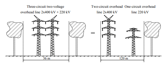
This year, 25th of January 2019, the record peak power demand 26,504 MW in the Polish power system occurred. The previous maximum power demand, which amounted 26,448 MW [1], was noted 28th of February 2018. The growing up demand for electric power extorts growth of generation sources and also lines and structures of the transmission system. Overhead power lines are the biggest and most extensive element of the transmission system fulfilling one of basic and the most important roles of any power system: they make possible electric energy transmission for the big distance. To find a territory for power network enlargement is the most difficult task. That suggests use multi-circuit lines. An additional advantage of this solution is enlargement of the transmitted power in the given section because of bigger number of circuits. The multi-circuit multi-voltage power lines in which at least two circuits placed on the common structure, have different voltage rating are also an interesting solution. Such an approach allows considerably reduce a width of the technological band, what illustrates the Fig. 1.
Fig.1. Comparison of widths of technological bands: three-circuit multi-voltage line 2×400 kV + 220 kV with two lines – two-circuit 2×400 kV and a single circuit 220 kV [2]
Multi-circuit multi-voltage overhead power lines have many advantages which cause, that their significant increase as well in Poland as in the world is observed.
An appearance of new elements of the subtransmission networks, i.e. multi-circuit and multi-voltage overhead power lines, carry with it necessity of their appropriate description using a mathematical model. The appropriately made mathematical model with defined and determined parameters takes into consideration all substantial features, phenomena and interactions occurring during operation of the object. In the paper as a mathematical model are understood admittance matrices of symmetrical components, which describe properties of the overhead line, where values of the admittance matrices are made dependent on earth-return circuits’ parameters, determined from geometry and material constants of circuits. In the paper attention was devoted mainly to zero model of overhead power line. An admittance model of the two-circuit single-voltage overhead line is well-known, therefore relationships which allow to determine a three-circuit multi-voltage line considering appearance of overhead earth wires and bundle conductors, are worked out and presented within the frames of the paper.
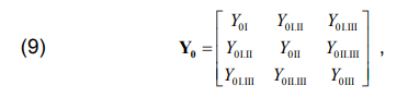
A computational model of the overhead line – earth-return circuits
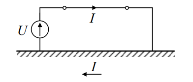
Creation of overhead lines’ mathematical models is based on the earth-return circuits’ theory. An earth-return loop was schematically shown on the Fig. 2.
Fig.2. An earth-return circuit
In earth-return circuits the earth treated as a homogeneous semiconducting space is a return conductor; phase conductors and earth wires are treated as parallel running closed earth-return loops. In this part of the paper the term of impedance of conductors which appears in earth-return circuits was discussed in order to understand an origin of particular components in final relationships.
The earth-return circuits are described by impedances: own W and mutual M. The own impedance is connected with an appearance of electromagnetic field penetrating inside of the conductor and also with inducing of electric rotational field around the discussed conductor because of current flow.
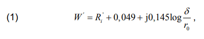
An own specific impedance of a single conductor amounts (in Ω/km) for frequency 50 Hz [3]:
.
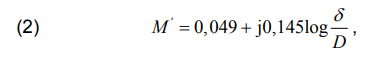
where Ri’ – own specific resistance of the conductor (in Ω/km), δ – distance of the discussed overhead conductor from the fictitious equivalent conductor placed in the earth (in m), r0 – characteristic radius of a single conductor (in m).
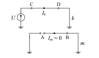
A mutual impedance is connected with influence of different conductor(-s) on the discussed overhead conductor. This mutual impedance is defined as a quotient of the potential difference in the section AB of the conductor and the current Ik(Fig. 3).
Fig. 3. The closed circuit with a current and the opened circuit
A mutual specific impedance for frequency 50 Hz amounts [3]:
.
where: D – geometrical distance between the discussed conductors k and m.
Zero model of a two-circuit overhead line
In course of considerations the following assumptions with relation to the system have been made [4]:
– the line is a linear element and appearing in it voltages and currents are mutually linear combinations, – the line conductors create with the earth earth-return circuits, – the line has a phase symmetry, – the line is symmetrical with regard to its ends, – capacities and leakages were passed over.
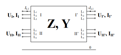
In order to obtain a mathematical model the line was treated as a multi-gate element where number of terminals is equal the number external nodes of the line. For two-circuit line after creation of the reference node, what means transfer its impedance to the phase conductors, it is obtained the scheme as in Fig. 4, being the twelve-node circuit [4].
Fig.4. A block diagram of the two-circuit line
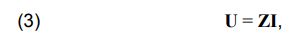
A basic dependence between values of currents and nodal voltages is given by the relation (3):
.
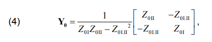
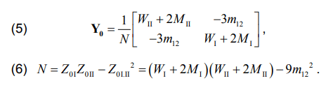
and the matrix of coefficients Z has a degree 12×12 in the case of two-circuit line. An adequate ordering the own and mutual line impedances, taking into consideration assumptions of symmetry, and passage to symmetrical components results obtaining only admittance matrix of positive components Y1 and negative Y2, which are the diagonal matrices, and also null matrix Y0(the mutual matrices between particular components do not appear). The matrix Y0 has form:
.
or taking into consideration the adequate own and mutual impedances:
.
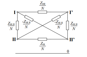
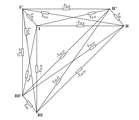
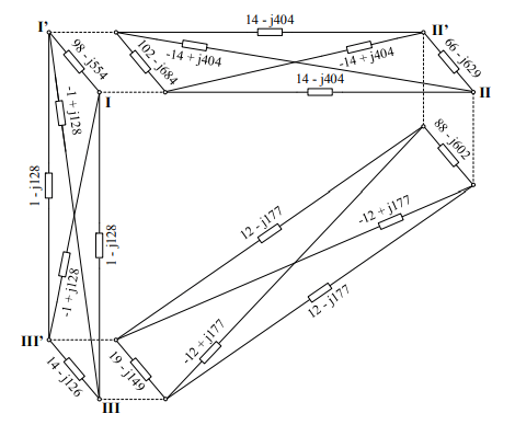
The matrix Y0 is represented by a zero scheme of the two-circuit line (Fig. 5) named an envelope scheme [5].
Fig.5. An equivalent zero scheme of the admittance of the two-circuit line
A mathematical model of the three-circuit overhead line
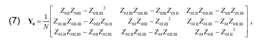
As result of the taken assumptions the analogous deliberations for the three-circuit line presented as an eighteen-node circuit lead to obtaining the admittance matrix of the zero-sequence component Y0 described by the relation (7):
.
and
.
The admittance zero matrix Y0 takes the form:
.
and the adequate scheme is shown in the Fig. 6:
Fig.6. An equivalent zero scheme of the admittance of the three-circuit line [6]
A zero model of the real three-circuit two-voltage overhead line
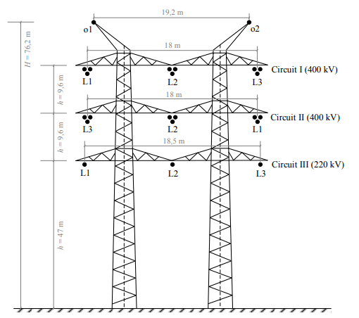
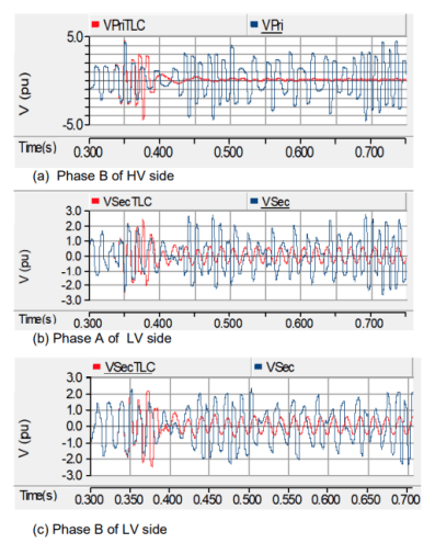
The obtained mathematical model was used to describe the real two-voltage three-circuit overhead line operating in the area of the PSE-South, located nearby the Łagisza station. The analysed is a type of EHV+EHV (2×400 kV + 220 kV) length 4,81 km, with a horizontal phase conductor configuration. Phase conductors for 400 kV circuits are a type of AFL-8 3×350 mm2 , for 220 kV circuit are of type AFL-8 525 mm2 , and earth wires AFL-1,7 95 mm2 .
A silhouette and geometrical parameters of tension supports of the deliberated three-circuit line are shown in the Fig. 7.
Fig.7. A scheme of silhouette of the tower of the two-voltage three-circuit line
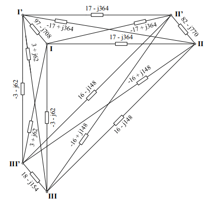
Thanks to a knowledge of the geometrical and material parameters the equivalent zero scheme was determined and shown in the Fig. 8. In calculations it was taken into account the influence of the earth wires by including their own and mutual impedances to the impedances of the phase conductors (a way of this including is given (among others) in [4], [7]). An appearance of the bundle conductors was also taken into consideration their aggregation to one equivalent conductor. Because of differentiated levels of rated voltages of circuits the line parameters were given per-unit and as a reference power was taken value of 100 MV·A. As reference voltages were taken rated voltages of particular circuits of the line.
Fig.8. A zero scheme of the real two-voltage three-circuit overhead line operated at the Łagisza station (parameters in pu)
An impedance asymmetry of the real line
The real line is usually not symmetrized (concerning the impedances) by transposition of phase conductors. It is caused by a big number of the necessary transpositions (full symmetrization of the three-circuit line needs 27 transpositions) and first of all by technical difficulties in carrying out the full transposition in the line.
In order to estimate an impedance asymmetry of the line a model without symmetrization was determined. A distinctive feature of the model is appearance of mutual impedances for symmetrical components between each pair, that means an appearance of voltages of all components at the current flow of only one component in the line (i.e. a symmetrical current).
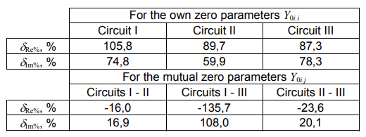
An influence of the impedance asymmetry of the analyzed line was determined by calculating voltages at the end of the line supplied with the symmetrical voltage of the positive sequence and charged with the current of the only positive sequence component. As a measure of the voltage asymmetry was taken a voltage asymmetry index α2% defined as a quotient of a value of a negative component of voltage and a value of a positive component and also unbalance index α0% defined as a value of a zero component of voltage to a positive component. Results for two different loads are presented in the table 1.
Table 1. Indices of asymmetry and unbalance of voltages in the three-circuit line with no transposition for different loads
.
The presented in the table 1 results show, that an impedance asymmetry of the line with no transpositions is not significant, because even at the full admissible load in all circuits (what does not happen in practice) maximal index amounts 0,33%. The similar results were presented in [8] for the two-circuit line. But it must be noticed that the analyzed section of the three-circuit two-voltages line is very short (4,81 km). In the case of longer lines the asymmetry indices can reach a boundary values which are given in operational and exploitation directions of particular networks. In the discussed case, at the predetermined construction of the tower and the used conductors, for the line length equal 25 km value of the asymmetry index reaches 2%.
Another way of estimation of influence of lack of transpositions is analysis of values of own impedance matrices for symmetrical components. Because transformation of the phase impedance matrix into the symmetrical components matrix is aimed to diagonalize the impedance matrix (what takes place in case of symmetrical phase impedance matrix) therefore from attributes of own values results that values of particular symmetrical components are equal the own values of this matrix. In case of lack of symmetrization of the phase matrix its own values are different. In the analyzed case the maximum relative error in the module of differences between the own values determined for the case with the phase transposition and without it amounts about 10% what means, that differences in particular impedances can be quite significant, what in turn can influence values of fault impedances calculated in such schemes [9].
A full zero model of the line and the simplified zero model
On account of a big complexity of a zero model the simplified model compound from three separate envelope models for each pair of circuits of the line, i.e. I with II, II with III and I with III. This simplified model being a connection of three individual envelope models was presented on the Fig. 9.
In order to compare the both models the percentage relative errors were determined after relations (10) and (11):
.
where: δRe% – the percentage relative error for the real part (in %); δIm% – the percentage relative error for the imaginary part (in %); index U means parameter of the simplified model, index D – of the exact model i, j – numbers of circuits; i, j ∈ {I, II, III}
Fig. 9. A simplified zero scheme of the two-voltage three-circuit overhead line (parameters in pu) [6]
The table 2 includes values of the relative error resulting from use of the simplified model. The simplified model significantly differs from the exact model, as for own as for mutual parameters. Errors in determination of particular parameters can exceed 100%. It means that the simplified model can not be applied as an substitute of the exact model.
Table 2. Relative percentage errors resulting from application of the simplified model [6]
.
Summary
A continuous development of the multi-circuit multi-voltage overhead line results in necessity of their adequate description. The determined nodal admittances of the three-circuit multi-voltage overhead line expresses structure and parameters of this element of the network, therefore allows to describe it precisely in the power system’s structure. Thanks to this the mathematical model can be used for representation of steady states without significant phase asymmetries or quasi-steady states at simplified short-circuit calculations.
An analysis of the lack of transpositions (i.e. symmetrization of the line) by determination of asymmetry and unbalancing indices for only the positive component of the load current showed that even big values of the current do not cause the significant voltage asymmetry. Nevertheless taking into consideration a development of the analyzed lines and perspectives of growth of their length, it can be expected an increase of the discussed asymmetries.
It seems to be necessary to continue analyses of importance of the impedance asymmetry in the multi-circuit overhead lines all the more that their constructional solutions are significantly differentiated. The investigated real three-circuit two-voltage line has relatively low geometrical asymmetry. Other solutions, presented e.g. in [2] are more asymmetric.
The carried on deliberations on possibility of creation of the simplified zero model showed, that the model compiled from three independent envelope models for each pair of the three circuits of an overhead line is characterized by significant errors (tabl. 2). This means that phenomena and couplings which take place during operation of the overhead line were not sufficiently taken into consideration. The simplified model takes into consideration only the “direct” impacts: circuit I for the circuit II, circuit II for the circuit III etc., but omits the “indirect” influences, i.e. e.g. circuit I for the circuit II through the circuit III. The obtained results testify that it is a significant circumstance and considerably influence the obtained values of parameters of the model. As result the simplified model does not fully renders properties of the overhead line and can not be an alternative for the exact model.
REFERENCES
[1] Strona internetowa Polskich Sieci Elektroenergetycznych S.A. http://www.pse.pl [2] Kumala R., Identyfikacja zakłóceń w wielotorowych różnopoziomowych napięciowo liniach elektroenergetycznych, Rozprawa doktorska, Gliwice 2016 [3] Kosztaluk F., Flisowski Z., Metody analizy układów przewódziemia, Przegląd Elektrotechniczny, 10/2001 [4] Bernas S., Ciok Z., Modele matematyczne elementów systemu elektroenergetycznego, Wydawnictwo Naukowo-Techniczne, Warszawa 1977 [5] Kacejko P., Machowski J., Zwarcia w systemach elektroenergetycznych, Wydawnictwo Naukowo-Techniczne, Warszawa 2013 [6] Dziendziel A., Wielonapięciowe elektroenergetyczne linie napowietrzne, Praca dyplomowa magisterska, Gliwice 2018 [7] Żmuda K., Elektroenergetyczne układy przesyłowe i rozdzielcze. Wybrane zagadnienia z przykładami, Wydawnictwo Politechniki Śląskiej, Gliwice 2014 [8] Robak S., Pawlicki A., Pawlicki B., Asymetria napięć i prądów w elektroenergetycznych układach przesyłowych, Przegląd Elektrotechniczny, 07/2014 [9] Miller P., Wancerz M., Wypływ sposobu wyznaczania parametrów linii 110 kV na dokładność obliczeń sieciowych, Przegląd Elektrotechniczny, 04/2014
Authors: dr hab. inż. Henryk Kocot, prof. PŚ, Politechnika Śląska, Instytut Elektroenergetyki i Sterowania Układów, ul. Krzywoustego 2, 44-100 Gliwice, E-mail: Henryk.Kocot@polsl.pl;. mgr inż. Agnieszka Dziendziel, doktorantka w Politechnice Śląskiej, Instytut Elektroenergetyki i Sterowania Układów, ul. Krzywoustego 2, 44- 100 Gliwice, E-mail: Agnieszka.Dziendziel@polsl.pl
Source & Publisher Item Identifier: PRZEGLĄD ELEKTROTECHNICZNY, ISSN 0033-2097, R. 95 NR 12/2019. doi:10.15199/48.2019.12.58
Published by A. M. Shiddiq YUNUS1, Ahmed Abu-SIADA2, Mohammad A.S. MASOUM3, State Polytechnic of Ujung Pandang, Indonesia (1), Curtin University, Australia (2), Utah Valley University , USA (3)
Abstract. Wind turbine generator (WTG) installation has been rapidly growing globally in the last few years. In the year of 2017, the WTG installation has reached a global cumulative installation of about 539 GW. Among several types of WTG, the doubly fed induction generator (DFIG) has been taking a large portion of the overall WTG installation since 2004. This popularity is due to the DFIG several advantages that include more extracted energy when compared with the fixed speed type and low cost due to the one-third size of the used converters when compared to the full converter type. However, the DFIG is vulnerable to grid faults. In this paper, a new application of Vector Based Hysteresis Current Regulator (VBHCR) of STATCOM is introduced to enhance the dynamic performance of DFIG-based wind turbine farm. The system under study is investigated using Matlab. Robustness of the proposed VBHCR is investigated through exploring the system performance under various levels of voltage sags. Simulation results show that for certain level of voltage sags at the point of common coupling (PCC), VBHCR-STATCOM can effectively improve the performance of the DFIG. As a result, voltage profile at the PCC can comply with the fault ride through codes of Spain to avoid the disconnection of the DFIGs from the grid.
Streszczenie. Zaprezentowano nowy sterownik do turbiny wiatrowej DFIG – Vector Based Hysteresis Current Regulator VBHCR systemu STATCOM umożliwiający poprawę dynamiki. Zbadano pracę układu przy różnych poziomach zapadu napięcia. Stwierdzono poprawę dynamiki i zabezpieczenie przed odłączeniem generatora od sieci. Nowe zastosowanie regulatora VBHCR systemu STATCOM do poprawy dynamiki generatora DFIG,.
Keywords: DFIG, Wind Energy, Vector Based Hysteresis Current Regulator, STATCOM. Słowa kluczowe: turbina wiatrowa, generator DFIG, STATCOM, regulator VBHCR.
Introduction
Installation of renewable energy-based power plants has been tremendously increased over the past decade to fulfil the target of generating 25% worldwide electric power from renewable energy by in 2025 [1].
As reported by the Global Wind Energy Council [2], about 539,123 MW of wind based power plants were installed worldwide by the year 2017. In UE, offshore wind farms are expected to growth by about 65GW by 2030 [3]. There are several types of WTG available in the market, for example Permanent Magnet Synchronous Generator (PMSG) [4], fixed speed [5] and Doubly Fed Induction Generator (DFIG). Among them, DFIG has become the most popular type that dominated the worldwide installation by 64% in the year 2016 [6]. This is attributed to the several advantages that a DFIG exhibits which include low converters ratings and more energy harvesting.
Although DFIG is designed to maintain acceptable performance during wind speed fluctuation through its pitch control mechanism, it is vulnerable to grid faults [7]. Therefore, some countries employ a strict grid code to avoid any damage to the wind turbine generator during certain levels and duration of grid faults. An example of the fault ride through (FRT) grid code for Spain wind power installation is shown in Figure 1 [8].
Fig.1. Fault Ride Through of Spain [8]
Figure 1 specifies three main areas of wind power operation [8]. Area “A” indicates the maximum voltage rise of the FRT of Spain, where it allows 130% voltage rise lasting for 0.5s duration and 120% for the next 0.5s. Area “B” in the other hand indicates the normal condition of FRT of Spain. Any voltage variation within ±10% (90-110%) is allowed within this area. The minimum voltage threshold limit and duration are specified in Area “C”. Within this area, a minimum threshold voltage of 50% lasting for 0.15s is permitted which is then gradually an increase to a voltage level of 90% after 15 seconds. Any voltage drop below Area “C” will lead to the disconnection of WTG from the grid.
Several papers to improve the control system for DFIG to comply with the grid codes can be found in the literatures [9-13]. However, all presented techniques are only suitable for the new installations. Owing to the fact that there is several of first generation of DFIG already installed worldwide since 2000s, therefore, an external compensator has become a better solution to improve the FRT capability of such WTGs.
References [14, 15] introduce the application of superconducting magnetic energy storage (SMES) unit on WTGs-grid connected to compensate the voltage at the point of common coupling (PCC) during grid faults. However, SMES unit is still an expensive technology due to the cryogenic system required to maintain the coil within superconducting state. The application of static synchronous compensator (STATCOM) in DFIG has been presented in [16-19]. In [17], application of the STATCOM was only limited for full converter-based wind energy conversion systems (FC-WECS). The main focus of [18] is the investigation of power electronic switching faults on the overall performance of the DFIG which might not cost effective as switching fault is a rare fault event. In [19], the study was limited to the voltage at the PCC without considering other important parameters such as the dc-link voltage, generated power and rotor speed.
The new idea presented in this paper is to employ a vector based hysteresis current regulator (VBHCR) to control the operation of a STATCOM connected to a DFIG-based WECS. Simulations are carried out using Simulink/MATLAB and the results are investigated and analysed considering the Spain FRT grid code [8]. The performance and robustness of the proposed VBHCR and the PCC voltage profile are examined under various levels of voltage sags.
System under Study
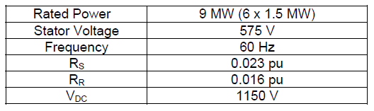
The system under study as shown in Fig. 2 consists of 6 x 1.5 MW DFIG that is connected to the grid via two transformers and a 30 km distribution line. The STATCOM is connected at the PCC via a step-up transformer. All system parameters are listed in Tables 1 and 2.
Fig.2. System under study
Table 1. Parameters of DFIG
.
Table 2. Parameters of Transmission Line
.
The DFIG system (Fig. 3) consists of two converters linked by a DC link capacitor to connect the rotor windings of the induction generator to the PCC transformer that is also connected to the induction generator stator windings.
Fig.3. Typical system of a DFIG
Vector based hysteresis current regulator based STATCOM
The concept of Equidistant-Band Vector Based Hysteresis Current Regulator (VBHCR) is introduced in [20] where the VBHCR is employed for both DFIG converters; Rotor Side Converter (RSC) and Grid Side Converter (GSC). Equidistant-Band VBHCR features a better steady state performance including fast transient response, adaptable to machine parameter variations and simple control algorithm. As mentioned above, designing new controller for the existing DFIG installation may not be cost effective. Therefore, the utilisation of VBHCR-STATCOM as an external compensator could be a practical and economical solution for the existing DFIG systems.
Proposed VBHCR of STATCOM for DFIG Applications
The proposed VBHCR for STATCOM is shown in Fig. 4. In this controller, a dq-abc transformation is applied, where d-q axes reference currents Id* and Iq* are generated from the error signals of the voltage across the DC link (ΔVdc), the voltage at the PCC (ΔVs) and two conventional proportional-integral (PI) controllers. The output current of the dq-abc transformation is compared with the line currents to generate an error current signal (ΔIabc) that is fed to the VBHCR to generate appropriate switching signals to the STATCOM switches. To eliminate the interference between phases (referred as inter-phases dependency) and maintain the advantages of the hysteresis controller, a phase-locked loop (PLL) technique is employed.
Fig.4. Typical VBHCR-STATCOM
The key point of VBHCR principle is based on the use of switching table for the VSC (shown in Table 2) of the proposed VBHCR as detailed discussed in [20]. Before fed into the switching table, the digital outputs of comparators (Dx and Dy) are created from four-level hysteresis comparator for x-axis and three-level hysteresis for y-axis. The practical proposed VBHCR is shown in Fig. 5.
Fig.5. Typical Implementation of Equidistant-Band VBHCR [20]
Results and Discussion
In order to investigate the robustness of the proposed STATCOM controller for DFIG applications, various case studies and scenarios are investigated.
Case Study 1: A Moderate Voltage Sag of 0.7 per-unit at the Grid Side
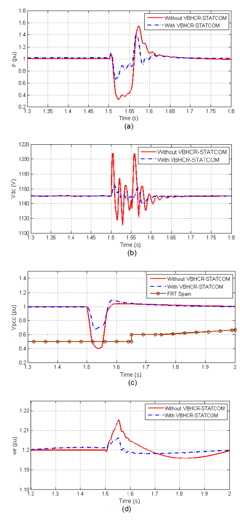
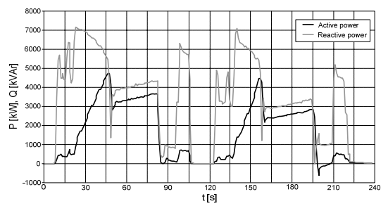
In this case study, grid voltage sag of 0.7 pu is applied at 1.5s and cleared out at 1.55s. Simulation results for this case study are shown in Figure 6.
Fig.6. Dynamic responses of DFIG with and without VBHCR-STATCOM for magnitude sag of 0.3 pu; (a) Output power; (b) Vdc-link profile; (c) Voltage profile at PCC and (d) Rotor Speed (ωr)
As shown in Fig. 6(a), without the proposed VBHCR-STATCOM, the output power tends to drop to a level less than 0.4 pu. This drop is compensated when the VBHCRSTATCOM is connected to the PCC to reach a level of 0.8 pu. Fig 6(b) reveals that without VBHCR-STATCOM, the voltage across the DC link will exhibit rapid oscillations due to a voltage dip at the grid side. With the proposed VBHCR-STATCOM connected to the system, this oscillation can be significantly damped. It is worth noting that significant oscillations in the DC link voltage may cause the protection system to block the converter operation [7]. As can be seen in Fig. 6(c), the voltage at the PCC exhibits 0.6 pu voltage sag and drops to a level of 0.4 pu during the fault duration. Compared with the FRT code of Spain, this level violates the minimum threshold voltage limit allowed by this code. When the VBHCR-STATCOM is connected to the PCC, the reactive power compensation by the STATCOM elevates this voltage to a level of 0.5 pu which is a safety accepted limit by Spain FRT code. Due to the drop in the generator active power, the shaft speed (ωr) accelerates as shown in Fig. 6(d) and reaches a crest value of 1.215 pu and takes a long time to settle down to the nominal value after fault clearance. With the connection of the VBHCR-STATCOM, both maximum overshooting and settling time are substantially reduced.
Fig.7. Dynamic responses of DFIG with and without VBHCR-STATCOM with magnitude sag of 0.1 pu; (a) Output power; (b) Vdc-link profile; (c) Voltage profile at PCC and (d) Rotor Speed (ωr)
Case Study 2: A Large Voltage Sag of 0.9 per-unit at the Grid Side
To investigate the capability of the proposed STATCOM to perform under large voltage sag levels, the level of sag at the grid side is increased to 0.9 pu. As can be seen in Fig. 7 (a), the power output of the DFIG is significantly dropping to almost zero level within the duration of fault. When the VBHCR-STATCOM connected to the system, the output power drop can be compensated by about 50%, which implies that the DFIG can contribute about 50% active power during the fault event. This is a momentous advantage of the proposed VBHCR-STATCOM.
Fig. 7 (b) shows the significant oscillations that the DC link voltage profile will exhibit if the proposed controller is not adopted. With the VBHCR-STATCOM connected to the system, the maximum overshooting and oscillations of the DC link voltage will be significantly damped. For a gird voltage sag of 0.9 pu, the voltage at the PCC will be reduced by about 0.7 pu and violates the low voltage limit of the Spain grid code as shown in Fig. 7(c).
Whereas with the connection of the proposed compensator, this level will be raised to a safe value (0.6 pu) which complies with the Spain codes requirement. Without the VBHCR-STATCOM, the rotor shaft speed exhibits a significant maximum overshooting during the fault and a long settling time after fault clearance. Both parameters are greatly enhanced when the proposed VBHCR-STATCOM is connected as shown in Fig. 7(d). This is a further contribution of the proposed VBHCR-STATCOM.
Conclusion
This paper presents a new application of the Vector Based Hysteresis Current Regulator (VBHCR) on STATCOM to improve the low voltage ride through capability of DFIG-based WECS. For the moderate and high voltage sag levels investigated in this paper, the following main conclusions can be drawn:
• Without employing any compensator, the performance of a DFIG-based WECS will be significantly degraded due to voltage sag events at the grid side. As a result of such faults, the generated power of the DFIG drops, voltage across the DC link exhibits significant oscillations, voltage at the PCC may violate the minimum threshold limit of the grid code, and rotor shaft speed accelerates affecting overall system stability.
• The proposed VBHCR-STATCOM acts to compensate the power at the point of common coupling during fault events. This results in maintaining system parameters such as the generated power and voltage at the PCC at accepted limits that allows the DFIG to support the grid during fault events rather than disconnecting it.
Acknowledgment: First author would like to thank Research, Technology and Higher Education Ministry of Indonesia for supporting the Research.
REFERENCES
[1] Ghislaine Kieffer, Toby D. Couture, Renewable Energy Target Setting, International Renewable Energy Agency (IRENA), June (2015). [2] Anenomous, Global Wind Statistic (2017). [3] M. Seghidi, M. Moradzadeh, O. Kukrer, M. Fahrioglu, Simultaneous Optimization of Electrical Interconnection Configuration and Cable Sizing in Offshore Wind Farms in Journal of Modern Power Systems and Clean Energy (2018), Vol.6, Issue:4, pp.749-762. [4] R. A. Priya, D. Dhanasekaran, P.C. Kishoreraja, Performance analysis of PMSG based wind energy conversion system using two stage matrix converter, Przeglad Elektrotechniczny (2019), Issue: 2, Pg. 112. [5] J. Pedra, F. Corcoles, LI. Monjo, S. Bogarra, A. Rolan, On fixed-speed WT generator modeling for rotor speed stability studies, IEEE Trans. on Power Syst. (2012). Vol. 27., Issue: 1, pp. 397-406. [6] C. Vázquez Hernández, T. Telsnig, A. Villalba Pradas, C. Vazquez Hernandez, T. Telsnig, and A. Villalba Pradas, JRC Wind Energy Status Report 2016 Edition (2017). [7] V. Akhmatov, Analysis of dynamic behaviour of electric power systems with large amount of wind power, PhD Theses (2003). Technical University Denmark. [8] M. Altin, Ö. Göksu, R. Teodorescu, P. Rodriguez, B. B. Jensen, and L. Helle, Overview of recent grid codes for wind power integration in Proc. Int. Conf. Optim. Electr. Electron. Equipment, OPTIM, (2010), pp. 1152–1160. [9] J. Lopez, E. Gubia, E. Olea, J. Ruiz, and L. Marroyo, Ride Through of Wind Turbines With Doubly Fed Induction Generator Under Symmetrical Voltage Dips, IEEE Trans. Ind. Electron., (2009) vol. 56, no. 10, pp. 4246–4254. [10] A. Bektache, B. Boukhezzar, Nonlinear predictive control of a DFIG-based wind turbine for power capture optimization, Electrical Power and Energy Systems (2018), Vol. 101. 92-102. [11] H. Mahvash, S. A. Taher, M. Rahimi, M. Shahidehpour, Enhancement of DFIG performance at high wind speed using fractional order PI controller in pitch compensation loop, Electrical Power and Energy Systems (2019), Vol. 104. pp. 259-268. [12] F.E.V. Taveiros, L.S. Barros, F.B. Costa, Heightened state-feedback predictive control for DFIG-based wind turbines to enhance its LVRT performance, Electrical Power and Energy Systems (2019), Vol. 104. pp. 259-268. [13] S.K. Raju, G.N. Pillai, Design and implementation of type-2 fuzzy logic controller for DFIG-based wind energy systems in distribution networks in IEEE Trans. Sustain. Energy (2016), vol. 7, no. 1, pp. 345-353. [14] A. M. S. Yunus, A. Abu-Siada, and M. A. S. Masoum, Effects of SMES on dynamic behaviors of type D-Wind Turbine Generator-Grid connected during short circuit, IEEE Power Energy Soc. Gen. Meet. (2011), pp. 11–16. [15] I. Ngamroo, Optimization of SMES-FCL for Augmenting FRT Performance and Smoothing Output Power of Grid- Connected DFIG Wind Turbine, IEEE Trans. Appl. Supercond. (2016), vol. 26, no. 7. [16] A. M. S. Yunus, A. Abu-Siada, and M. A. S. Masoum, Effect of SMES Unit on the Performance of Type-4 Wind Turbine Generator during Voltage Sag, IET on Renewable Power Generation RPG (2011), pp. 94. [17] A. M. S. Yunus, M. A. S. Masoum, A. Abu-Siada, Effect of STATCOM on the Low-Voltage- Ride-Through Capability of Type-D Wind Turbine Generator, IEEE PES Innovative Smart Grid Technologies (2011), pp. 1-5. [18] A. F. Abdou, A. Abu-Siada, H. R. Pota, Application of STATCOM to improve the LVRT of DFIG during RSC fire-through fault, Universities Power Engineering Conference (AUPEC) 2012 22nd Australasian (2012), pp. 1-6. [19] Beheshtaein, Optimal Hysteresis Based DPC Strategy for STATCOM to Augment LVRT Capability of a DFIG Using a New Dynamic References Method, IEEE 23rd International Symposium on Industrial Electronics (ISIE) (2014), 612 – 619. [20] M. Mohseni, S. M. Islam, and M. A. S. Masoum, Enhanced hysteresis-based current regulators in vector control of DFIG wind turbines, IEEE Trans. Power Electron. (2011), vol. 26, no. 1, pp. 223–234.
Authors: Dr. A. M. Shiddiq Yunus is with Energy Conversion Study Program, Mechanical Engineering Department, State Polytechnic of Ujung Pandang, Makassar 90245, Indonesia, Email: shiddiq@poliupg.ac.id; Dr. Ahmed Abu-Siada is with Electrical and Computing Engineering Department, Curtin University, Perth 6102, WA, Australia, Email: A.AbuSiada@curtin.edu.au; Dr. Mohammad A.S., Masoum is with Electrical Engineering at Utah Valley University, Orem UT, 84058, USA, Email: mmasoum@uvu.edu.
Source & Publisher Item Identifier: PRZEGLĄD ELEKTROTECHNICZNY, ISSN 0033-2097, R. 96 NR 1/2020. doi:10.15199/48.2020.01.16
Published by Jake Hertz, EE Power – News: Researchers Achieve Higher Voltage PV With Inverter System, November 13, 2023.
A team of researchers claims to cut cable requirements by 700 kg of copper per kilometer of cable with a higher voltage inverter system for photovoltaics.
In photovoltaic (PV) systems, reducing cable size is essential for economic and environmental reasons. As PV installations scale to meet the growing demand for renewable energy, the quantity of cabling required multiplies. Thicker cables consume more copper, a material with significant cost and limited availability.
Installing PV panels. Image used courtesy of Oregon DOE
Efficient cable management through size reduction is a pivotal aspect of optimizing PV systems, ensuring they remain economically viable and sustainable. To this end, a group of researchers at the Fraunhofer Institute for Solar Energy Systems (ISE) recently developed an inverter system to enable significantly reduced cabling requirements in PV systems.
Higher Voltage, Smaller Cable
Reducing the cabling requirements is extremely important as PV systems scale up. To this end, a promising strategy is to increase the system voltages.
The principle behind this is rooted in the relationship between voltage (V), current (I), and power (P), as described by the electrical power formula P = V×I. When the voltage, V, is increased for a given power, the current required is reduced. Since the current carrying capacity of a cable is a determinant of its size, a lower current allows for the use of cables with a smaller cross-sectional area.
Smaller cables offer several advantages. First, they are less expensive because they use less material, which is particularly significant when considering precious resources like copper. The price of copper is subject to market fluctuations and has a notable impact on project costs. Reducing copper usage not only cuts costs but also eases the demand for this limited resource, aligning with sustainable resource management practices.
The modern power grid already employs a high-voltage power transmission scheme. Image used courtesy of Edison Tech Center
Second, reducing cable size has environmental benefits. The production of copper and other cable materials has an environmental impact, including energy consumption and greenhouse gas emissions. By using thinner cables, the environmental footprint of manufacturing, transporting, and disposing of these materials is reduced.
Lastly, high-voltage systems can transmit power more efficiently over long distances with reduced losses. This is because electrical power is also defined as P = I^2*R. Hence, at a higher voltage (i.e., lower current), the losses in power transmission are significantly reduced. This is impactful for renewable energy sources like solar and wind, which are often located far from consumption centers.
Fraunhofer’s Solar Inverter Study
In a recent study by the Fraunhofer ISE, the researchers developed the world’s first medium-voltage string inverter for large-scale PV power plants. Unlike conventional PV string inverters, which typically operate at lower output voltages of 400 VAC to 800 VAC, the solution from the study outputs voltage as high as 1,500 VAC @ 250 kVA.
Different cable cross sections for different voltages. Image used courtesy of Fraunhofer ISE
The team tackled the challenge by employing silicon carbide semiconductors, which possess a higher blocking voltage than traditional silicon semiconductors. The use of these advanced semiconductors was complemented by a novel cooling concept utilizing heat pipes, which enhanced the system’s efficiency and reduced the need for aluminum in its construction. By stepping up the voltage to the medium-voltage range, the inverter reduces the current for a given power output. This reduction in current directly translates to a decrease in the required cable size, yielding substantial cost savings and resource conservation.
According to the team, a traditional 250 kVA string inverter would necessitate cables with a cross-section of 120 mm², but with the medium-voltage inverter, the cable cross-section is reduced to just 35 mm². This reduction could save approximately 700 kilograms of copper per kilometer of cable.
Far-Reaching Implications of a Medium-Voltage Grid
The study’s success in feeding power into the medium-voltage grid is a testament to its practical viability. It paves the way for the next generation of large-scale PV power plants and sets a precedent for more resource-efficient energy system electrification. Importantly, the study’s implications extend beyond PV systems. The medium-voltage inverter concept can be applied to wind turbines, electric mobility, and industrial applications, where similar benefits in terms of resource efficiency and cost savings can be realized.
The researchers are now seeking partnerships with solar farm developers and grid operators to field-test their new concept, which could transform how we harness and distribute renewable energy.
Author: Jake Hertz has both his MS and BS in electrical and computer engineering from the University of Rochester. Hertz is a member of Tau Beta Pi, Phi Beta Kappa, and the NYC-based informal engineering collective. He has research and educational experience in fields including digital and analog IC design, hardware security, energy-efficient memory algorithms, and artificial intelligence. Outside of engineering, Hertz is a former collegiate baseball player and enjoys exercising, being in nature, or spending time with friends.
Published by Bartłomiej SZAFRANIAK, Paweł ZYDROŃ, and Łukasz FUŚNIK, AGH University of Science and Technology, Krakow, Poland
Abstract. In low-voltage (LV) electrical networks metal-oxide varistor (MOV) surge arresters connected in parallel are often used against overvoltages. The paper presents the results of laboratory experiments, during which pairs of parallel connected MOV surge arresters were subjected to surges of specified energy. The tests determined energy distribution between surge arresters for AC burst voltage stresses, temperatures recorded on their surface using contact sensors and temperature distribution images (IR thermograms). The analysis of results and conclusions are also presented.
Streszczenie. W sieciach niskiego napięcia stosowane są zwykle tlenkowe ograniczniki przepięć. W artykule przedstawiono wyniki badań, podczas których pary równolegle połączonych ograniczników poddano działaniu narażeń o określonej energii. Badano rozkład energii pomiędzy ograniczniki dla narażeń przebiegami AC oraz rejestrowano termogramy IR i temperatury na ich powierzchni, mierzone czujnikami kontaktowym. Przedstawiono analizę wyników badań i wnioski. (Analiza wpływu nierównomiernego rozpływu prądu na nagrzewanie się równolegle połączonych tlenkowych ograniczników przepięć niskiego napięcia).
Keywords: metal-oxide varistor, surge arrester, heating, parallel working, unequal current distribution. Słowa kluczowe: warystor tlenkowy, ogranicznik przepięć, nagrzewanie, praca równoległa, nierównomierny rozpływ prądu.
Introduction
The contemporary requirements for high reliability of electrical devices and instruments make it necessary to protect all apparatus working in electrical networks against voltage surges that can arise in them. Overvoltages arising and propagating in networks can cause unacceptable level of voltage stresses destructively acting on electrical insulation systems. For protection of electrical devices and proper insulation coordination, various methods of mitigation and limitation of surges are applied, depending on characteristic of occurring overvoltages and specific properties of protected objects [1-7]. Currently, the most commonly used solution for this purpose is the use of surge arresters containing ZnO metal-oxide varistors (MOSA – Metal Oxide Surge Arrester) as voltage limiting devices. MOSAs are used at all voltage levels, from low voltage (LV), through medium voltage (MV) up to high (HV), extraand ultra-high (EHV and UHV) voltages.
The physical mechanism of electric current conduction in the varistor is complex due to the influence of the varistor material properties and non-linear phenomena occurring at the boundaries of grains that build its polycrystalline structure [8-10]. The observed result is a non-linear dependence of the current flowing through the varistor from the voltage applied to its electrodes, which makes it very useful as a voltage stabilizing element. The strongly nonlinear current-voltage (or electric field E – current density J, Fig. 1) characteristic of the MOV is described by the formula:
.
where: I – current flowing through the varistor; V – voltage on the varistor; k, α – constants, depending on the materials and parameters of the varistor production process.
In the pre-breakdown range of ZnO varistor current-voltage characteristic (Fig. 1), the resistive component of the varistor leakage current is many times smaller than the capacitive one. Experimentally observed static current-voltage characteristics in this region are almost linear (ohmic-type) but simultaneously very sensitive on the temperature of the varistor. Because of physical mechanism, resistive current increases significantly together with increase of varistor temperature.
In the voltage stabilization range of ZnO varistor currentvoltage characteristic, clamping voltage shows a relatively small change in the wide range of varistor currents. For very large currents, in the saturation range, the increase of the voltage on the varistor is the result of the ZnO grain resistivity influence.
Fig.1. A typical E = f (J) characteristic of zinc oxide varistor
Varistors are usually produced in the form of discs. Disc thickness determines the clamping voltage value and its circular area the highest value of the surge current, so the volume of a disk is related to the varistor energy absorption capacity. To improve the overvoltage protection of devices installed in electrical networks and increase the capacity to absorb energy of overvoltages MOSAs are used in parallel, and are placed in different points of an electric network (at terminals of protected devices) or multiplied at terminals of a single protected device. The last one solution in practice causes problems with equal overvoltage energy dissipation, related to the differences in current-voltage characteristics of parallel mounted varistors [11-15].
Paper presents the results and analyzes of experimental investigations carried-out on the two parallel connected low voltage MOSAs of the same type, subjected to the sequence of AC voltage bursts stressing structures of their varistors. The results of voltage and currents measurements and evaluated energies absorbed by each MOSA as well as the temperature changes recorded by two methods on the surfaces of the arresters enclosure are presented and discussed.
Tested objects, experimental setup and procedure
A. Tested objects
For the laboratory experiments were used commercially available low voltage MOV surge arresters (Fig. 2) with the basic technical parameters presented in Table 1.
Fig.2. Tested low voltage surge arresters with a polymer housing
Table 1. Selected parameters of tested MOSA
.
B. Experimental setup
Used during laboratory experiments system for testing of parallel connected low-voltage MOSAs (Fig. 3, 4, 5) allowed generation of voltage waveforms of AC burst in programmed time sequences. During the tests, the digital storage oscilloscope (Tektronix TDS 784D) recorded the following waveforms: voltage at surge arresters (Ch1) and currents of each of two arresters (Ch2 / Ch3); indirectly by measuring of voltages on two precision 4-terminal 0.1 Ω resistors.
Fig.3. General scheme of laboratory system for testing of parallel-connected low-voltage MOSAs (ATR – autotransformer; SUTR – step-up transformer; IR-CAM – infrared camera; TMU – 2-channel temperature measurement unit; HV-D – high voltage divider).
The processes of heating and cooling of surge arresters subjected to voltage stresses of the AC burst sequence were observed by infrared camera to take thermograms of the MOSAs housing surfaces and by a contact temperature measurement system containing two K-type thermocouples. Both temperature measuring instruments were read using the USB serial interface (USB 1 / USB 2).
Fig.4. Measuring stand for parallel-connected LV MOSAs tests – general view
Fig.5. Tested LV MOSAs with a high voltage probe and two series-connected 4-terminal resistors used for measuring individual currents of parallel varistors
C. Laboratory experiment procedure
In the first stage of the test procedure, from the group of about twenty of the same type low voltage MOSAs, two arresters (signed as A and B MOSA) with noticeably different clamping voltage values were selected. Then, for their parallel connection, a programmed 50 Hz AC burst voltage sequence was realized. Each single AC voltage burst fed to the parallel connected surge arresters had a width of about 1.2 second. The entire energy pulses sequence contained five successive AC bursts, separated by a time interval of about 3 minutes. The first two were bursts with lower voltage and therefore also lower energy (respectively 100 J and 94 J). The next three were bursts with a slightly higher voltage, but with significantly higher energy (respectively 1326 J, 1360 J, and 1366 J).
Results of experiment
Figures 6 and 7 present digitally recorded waveforms of voltage and currents of surge arresters, acquired for low and high energy 50 Hz AC bursts during the test sequence. Table 2 summarizes the energy values absorbed individually by MOSAs A and B in the AC bursts sequence.
Fig.6. Recorded AC burst waveforms for low-energy stimulation: voltage (top), current of MOSA B (middle), and current of MOSA A (bottom)
Fig.7. Recorded AC burst waveforms for high-energy stimulation: voltage (top), current of MOSA B (middle), and current of MOSA A (bottom).
Table 2. Energy of AC bursts registered for MOSAs A and B
.
Figure 8 presents plots of the temperatures on the surface of MOSAs A and B, recorded using a measuring system with two K-type thermocouples. A significant temperature difference between these two surge arresters is visible, resulting from significantly different energy dissipated in them. The same effects can be seen when analyzing the results of infrared observation of the housing of the two tested MOSAs. Figure 9 shows the thermal state images of MOSAs A and B surfaces in the time moments corresponding to the points marked on the temperature plots in Figure 8.
Fig.8. Plots of the temperatures on the bottom surface of MOSAs A and B, recorded using a measuring system with two K-type thermocouples
Fig.9. MOSA A and B thermograms recorded by the infrared camera in the moments of time indicated in the temperature plots shown in Figure 8. (Note: temperature scales are not identical on all thermograms)
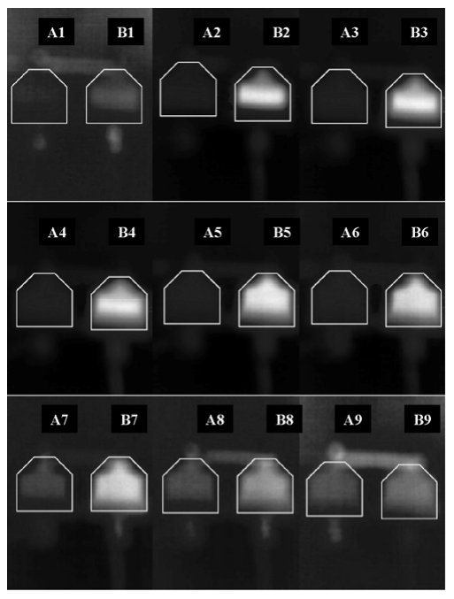
Discussion of results and conclusions
In the analyzed case, the energy distribution between A and B MOSAs ranged from approximately 1:3 for low energy AC bursts to approximately 1:4 for high energy ones. This indicates very unfavorable working conditions of the B arrester, dissipating the main part of the AC bursts energy.
The use of parallel connected MOSAs causes problems related to uneven distribution of surge currents between used protecting devices. This results in an uneven energy and thermal load of the varistors of individual arresters. The performed test confirms this problem for low voltage MOSAs of the same type, without the selection which allows proper cooperation of surge arresters with similar current-voltage characteristics.
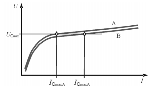
The strongly non-linear character of equation (1) causes that small differences in the parameters of two neighboring characteristics result in large difference of currents for the same voltage on parallel connected varistors (Fig. 10).
Fig.10. Influence of differences in current-voltage characteristics on MOSA A and B currents (UCmax – maximum value of clamping voltage; ICmaxA – MOSA A current at UCmax; ICmaxA – MOSA B current at UCmax)
The long time constant of the low voltage MOSA cooling process [17] causes that repeated energy stimulus successively accumulates its effect, raising the temperature of the varistors. Then, the uneven distribution of the dissipated energy accelerates thermal aging of the varistor of the more loaded surge arrester. To limit this phenomenon, you can:
1) make a selection of surge arresters connected in parallel in terms of high similarity of the currentvoltage characteristics;
2) use additional low value resistors connected in series with varistors, affecting the resultant currentvoltage characteristics [11]. Unfortunately, the second solution affects the overvoltage mitigation at protected devices in the same time.
Acknowledgement The presented researches were financed by the Polish Ministry of Science and Higher Education, by subvention for Faculty of Electrical Engineering, Automatics, Computer Science and Biomedical Engineering of AGH University of Science and Technology, Krakow, Poland.
REFERENCES [1] Hasse P., Overvoltage protection of low-voltage systems, 2nd ed., ISBN 978-0852967812, IET, 2000. [2] Paul D., Low-voltage power system surge overvoltage protection, IEEE Trans. Ind. Appl., 37 (2001), No. 1, 223–229 [3] Paolone M., Nuci C. A., Petrache E., Rachidi F., Mitigation of lightning-induced overvoltages in medium voltage distribution lines by means of periodical grounding of shielding wires and of surge arresters: modeling and experimental validation, IEEE Trans. Power Del., 19 (2004), No. 1, 423–431 [4] Jaroszewski M., Pospieszna J., Ranachowski P., Rajmund F., Modeling of overhead transmission lines with line surge arresters for lightning, International CIGRÉ Colloq., Cavtat, Croatia, May 2008 [5] Kuczek T, Stosur M., Szewczyk M., Piaseczki W., Steiger M., Investigation on new mitigation method for lightning overvoltages in high-voltage power substations, IET Gen., Transm. Distrib., 7 (2013), No. 10, 1055–1062 [6] Florkowski M., Furgał J., Kuniewski M., Propagation of overvoltages in distribution transformers with silicon steel and amorphous cores, IET Gener. Transm. Distrib., 9 (2015), No. 16, 2736–2742 [7] Szewczyk M, Kuniewski M, Controlled voltage breakdown in disconnector contact system for VFTO mitigation in gasinsulated switchgear (GIS), IEEE Trans. Power Del., 32 (2017), No. 5, 2360–2366 [8] Matsuoka M., Nonohmic properties of zinc oxide ceramics, Jpn. J. Appl. Phys., 10 (1971), No. 6, 736–746 [9] Eda K., Zinc oxide varistors, IEEE Electr. Insul Mag., 5 (1989), No. 6, 28–41 [10] Maran G. D., Levinson L. M., Philipp H. R., Theory of conduction in ZnO varistors, J. Appl. Phys., 50 (1979), 2799–2812 [11] Putrus G. A., Ran L., Ahmed M. M. R., Improving current sharing between parallel varistors, ISIE 2001 – IEEE Int. Symp. Industrial Electronics, Pusan, Korea, June 2001 [12] J. He, et. al, Electrical parameter statistic analysis and parallel coordination of ZnO varistors in low-voltage protection devices, IEEE Trans. Power Del., 10 (2005), No. 1, 131-137 [13] Tuczek M. N., Broker M., Hinrichsen V., Galer R., Effects of continuous operating voltage stress and AC energy injection on current sharing among parallel-connected metal–oxide resistor columns in arrester banks, IEEE Trans. Power Del. 30 (2015), No. 3, 1331-1337 [14] Tsujimoto Y., Tsukamoto N., Tsuge R., Baba Y., Surge withstand capability of parallel-connected metal oxide varistors, 34th Int. Conf. Lightning Protection ICLP 2018, Rzeszow, Poland, Sept. 2018 [15] Cuixia Z., UHV transmission technology, Elsevier Science Publishing Co Inc., ISBN: 978-0128051931, 2017 [16] Ahmed M.M.R., Putrus G.A., Ran L., Penlington R., Measuring the energy handling capability of metal oxide varistors, CIRED 2001 16th Int. Conf. and Exhib. on Electr. Distrib., Part 1: Contributions, IEE Conf. Publ. no. 482, Amsterdam, The Netherlands, June 2001 [17] Szafraniak B., Bonk M., Fuśnik L., Zydron P., Influence of high current impulses and 50 Hz AC bursts on the temperature of low-voltage metal-oxide surge arresters, 2018 Progress in Applied Electr. Engineering (PAEE), Koscielisko (Zakopane), Poland, June 2018
Authors: mgr inż. Bartłomiej Szafraniak, dr hab. inż. Paweł Zydroń, mgr inż. Łukasz Fuśnik, AGH University of Science and Technology, Dept. of Electrical and Power Engineering, al. Mickiewicza 30, 30-059 Kraków, Poland, E-mail: szafrani@agh.edu.pl, pzydron@agh.edu.pl, lfusnik@agh.edu.pl.
Source & Publisher Item Identifier: PRZEGLĄD ELEKTROTECHNICZNY, ISSN 0033-2097, R. 96 NR 1/2020. doi:10.15199/48.2020.01.11
Published by C. MADTHARAD, Provincial Electricity Authority (PEA), Thailand. and J. WARMAN, Senergy Econnect Australia. T&D World – Renewables: Thailand Integrates Large-Scale Wind Farms, Sept. 28, 2015.
Provincial Electricity Authority address power-quality issues that arise from increasing penetration of renewable energy.
In the Kingdom of Thailand, power-quality regulations applicable to small power producers and very small power producers were first issued in 2008. The regulations specify requirements for steady-state voltage, power factor, frequency, voltage fluctuations, harmonics and direct current.
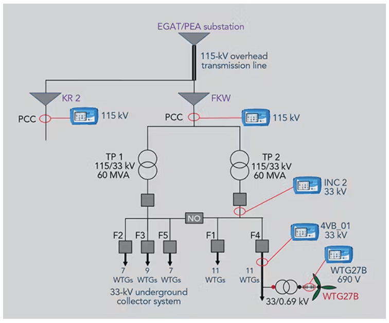
The Provincial Electricity Authority is responsible for carrying out the on-site power-quality testing of generator installations for all new small power producers and very small power producers prior to the plant entering commercial operation. In late 2012, the first large-scale wind farm in Thailand — the 90-MW FKW project — came on-line followed in early 2013 by the neighboring 90-MW KR2 wind farm. The impact on power quality attributable to these wind farms — the largest in Southeast Asia — required a number of mitigation measures to comply with the power-quality regulations of the Kingdom of Thailand.
Schematic diagram of the wind farm 115/33-kV network showing the location of the metering equipment to record power quality.
Pre-Grid Connection Monitoring
Power-quality monitoring results showed voltage fluctuation was not an issue as the wind turbine generators (WTGs) were decoupled from the grid by a fully rated converter. Also, the WTGs were designed to maintain voltage, power factor, frequency, voltage fluctuation and direct-current injection within acceptable levels. However, the harmonic current emissions and harmonic voltage distortion sometimes failed to comply with the regulation limits.
The total harmonic distortion in the voltage and the fifth harmonic current emission both exceeded the allowable limits under some operating conditions. The total harmonic voltage distortion exceeded the allowable limit during low wind speeds when the power output of the wind farm was between 0% and 30% of the installed capacity. The fifth harmonic voltage was the most significant in terms of exceeding the acceptable limit. The fifth harmonic current exceeded the limit when the wind farm power output was between 0% and 70% of the installed capacity.
The monitoring test results also revealed the fifth harmonic impedance changed dynamically depending on the wind speed and output power of the wind farm as the number of generators connected varied in accordance with the wind speed fluctuations across the wind farm site. Harmonics generated by the voltage source converter-based WTGs did not remain constant but varied according to the converter control and switching scheme.
Schematic diagram of the wind farm 115/33-kV network showing the location of the harmonic filters.
The Large-Scale Wind Farms
Each of the wind farms comprise 45 Siemens SWT-2.3-101 wind turbines. The 690-V WTG voltage is stepped up to 33 kV, and the transformer is connected to a 33-kV underground cable collector system. This system is connected to the Provincial Electricity Authority’s 115-kV overhead transmission line by two parallel 115/33-kV, 60-MVA power transformers at the wind farm substation. Each wind turbine has a rating of 2.3 MW and an aerodynamic rotor diameter of 101 m (331 ft). An asynchronous generator is decoupled from the grid by a fully rated frequency converter.
A wind turbine with an induction generator directly connected to the grid is not expected to create any significant harmonic distortions during normal operation. However, wind turbines with power electronic converters do produce harmonic current emissions, so the possibility of harmonic voltage distortion must be considered. The harmonic current emission of such wind turbine systems is normally included in the manufacturer’s power-quality data information. The anticipated harmonic voltages can be calculated from the harmonic current emissions of the wind turbine, but this requires knowledge of the grid impedances at different frequencies.
The harmonic signature of a WTG cannot be predicted by mathematical equations such as the Fourier analysis. As a result, it is necessary to investigate the harmonic profiles obtained from field measurements such that some commonalities can be determined for various turbine types and operating under variable conditions. Harmonics have the potential to excite an internal or external resonance point or even destabilize the system operation.
Fifth harmonic filter installed at the wind farm substation.
On-Site Monitoring Tests
To study the impact of the wind farms on power quality at all voltage levels, power quality meters were installed at four locations, namely at the point of common coupling (PCC) at 115 kV, the 33-kV collector system, and the input and output terminals of the 33/0.69-kV wind turbine transformer. The measurement recorder confirmed the active power at the PCC was proportional to the number of WTGs, while the reactive power from the WTGs was not proportional to the number of turbines. This varies as the reactive power at the PCC is controlled with a closed-loop controller, and the reactive power output of the WTG is varied to achieve the set point target at the PCC.
Three modes are available to control reactive power at the PCC: reactive power control mode, voltage control mode and power factor mode. The simplest strategy for the wind farm is to operate in the reactive power control mode with a 0-MVar set point to maintain unity power factor. In this mode, the wind farm will not export or consume reactive power when the turbines are operating. However, when this control strategy was adopted, there were some steady-state overvoltage problems at high active power output levels because the output reactive power of the wind farm was controlled to 0 MVar and used reactive power measured at the 115-kV side of the wind farm transformers as the feedback signal.
With this control strategy, if the wind speed is high enough for the wind turbines to go on-line, the converter imports reactive power, compensating for the capacitance of the underground cables in the collector system, to try to control the reactive power to 0 MVar at the PCC. If the wind is low, there may be only a few wind turbines on-line and the wind farm may export reactive power (<-4 MVar). If there is no wind, and the wind turbines are off-line, the quiescent reactive output from the wind farm as a result of the underground cables is around -4.0 MVar and the voltage is not actively controlled by the wind farm. In this situation, the voltage at the PCC may exceed the grid code limit of 1.05 p.u. (120.75 kV).
The wind farm substation 115-kV switchyard.
Operational Experience
Prior to Jan. 18, 2013, the wind farm always supplied reactive power to the utility, but following a change in the control mode from constant reactive power control to voltage control with a target voltage of 1.03 p.u. (118.4 kV), the wind farm supplied and absorbed reactive power from the utility. The results recorded indicated about +6.8 MVar was absorbed during maximum active power output generation and -4.1 MVar was supplied during low active power output generation.
Operationally, when the voltage fell below the target, the reactive export increased to support the voltage. When the voltage rose above the target, the reactive power import increased to reduce the voltage. With the wind farm operating in the voltage control mode, the steady-state voltage remained below the allowable maximum of 1.05 p.u.
The variable-speed wind turbines with fully rated frequency converters are capable of controlling the output of active and reactive power. It is possible to control the output reactive power appropriately with the variation of the output real power, so voltage changes from the real power flow may be compensated by the reactive power flow, minimizing the flicker emission.
The results recorded from Jan. 1, 2013, to Jan. 1, 2014, confirmed CP95 of the short-term flicker severity (CP95 of Pst=0.22) and long-term flicker severity (CP95 of Plt=0.46) — as per standard EN 50160 Voltage Characteristics in Public Distribution Systems, issued by the European Committee for Electrotechnical Standardization — complied with the limits in the regulations.
In the regulations, limits are specified for the total harmonic distortion in voltage and individual harmonic current emissions. However, on-site monitoring at the 115-kV PCC confirmed the harmonic distortion (THDv = 2.24%) and the fifth harmonic current emission (4.51 A) failed to comply with the regulations.
The results recorded from Jan. 1 through Jan. 31, 2013, showed the total harmonic distortion in voltage exceeded the limit at low wind speeds when the wind farm power output was between 0% and 30% of the installed capacity. The fifth harmonic current exceeded the limits for about 80% of the period when the wind farm output power was between 0% and 70% of installed capacity. These characteristics are attributable to the fifth harmonic impedance that changes dynamically depending on the wind speed and power output of the wind farm.
Harmonics generated by voltage source converter-based WTGs do not remain constant but will vary according to the converter control and switching scheme. To mitigate the harmonics issues, a fifth harmonic filter was installed downstream of one of the feeder circuit breakers supplying the 33-kV bus bar. These passive harmonic filters, which were retrofitted to existing substations, have mitigated the harmonics emissions successfully from the wind farms, allowing them to operate in compliance with the Kingdom of Thailand’s power-quality regulations.
Successful Mitigation
Government policy in Thailand is for renewable energy and alternative energy sources to account for 25% of the installed generation within the next 10 years. According to the country’s 2010 Power Development Plan Revision 3, the total installed generation capacity by the end of 2030 will be around 20,500 MW, including 3,800 MW of wind energy and 2,000 MW of solar energy, some 29% of the total generating capacity.
With the increasing penetration of renewable energy, the impact of power quality from the renewable generators will become increasingly important. Experience from the first two wind farm projects has demonstrated, with the appropriate design, negative impacts on power quality can be mitigated successfully.
Authors
Chakphed Madtharad (chakphed@gmail.com) graduated with a Ph.D. degree in electrical engineering from Chiang Mai University, Thailand, in collaboration with the University of Canterbury, New Zealand. He currently works in the smart grid planning division of the Provincial Electricity Authority, where his responsibilities include harmonics and power quality, power electronics, power system smart grids and microgrids.
Jeremy Warman (jeremy.warman@lr-senergy.com) was awarded a ME degree in electrical engineering from the University of Canterbury, New Zealand. He currently works for LR Senergy in Melbourne, Australia. Warman’s interests include harmonics and power quality associated with wind farms and renewable energy integration.
Published by Alex Roderick, EE Power – Technical Articles: Potential Transformer Operation, Applications and Accuracy, July 14, 2021.
Learn about the operation and accuracy of potential transformers.
The high voltages typically seen on power lines are a hazard to technicians working on or near the power lines. It is a difficult task to design a voltmeter to measure these high voltages. A potential transformer is primarily a precision two-winding transformer that is used to step down high voltage to enable safe voltage measurement.
Operations
The stepped-down voltage from a potential transformer can be measured directly with a voltmeter. The line voltage can be calculated by multiplying the measured voltage by the turns ratio of the transformer. However, a better solution is to use a modified voltmeter.
The display of the meter can be modified with a new meter face or programmed to show a value corresponding to the actual line voltage, even though a stepped-down value was actually measured. The meter can multiply the measured value by the turns ratio to display the actual line voltage.
The primary side of the potential transformer is connected across the power lines (See Figure 1). Fuses can be added for safety and to make it easy to remove the potential transformer from the circuit for maintenance. To ensure that the voltage measurement is as precise as possible, the load on the potential transformer must be kept to a minimum. The voltmeter should be a high-impedance model to draw as little current as possible from the transformer. This non-changing load keeps the voltage ratio constant, and as the primary voltage changes, the secondary voltage changes proportionally.
Figure 1. A potential transformer is used to step down the high voltage of a power line in order to make it easier to measure.
Potential transformers can be designed with almost any turns ratio so that the voltage can always be reduced to 120V. This allows standard voltage meters to be used. For example, a potential transformer with a turns ratio of 60:1 can be used to measure 7200V. The same meter can be used to measure 34.5kV if a potential transformer with a turns ratio of 287.5:1 is used to step down the line voltage to 120V. In this case, a different multiplication factor is used in the display or a different face installed on the meter.
Potential transformers are usually fairly small. They are typically rated at 500 VA or less. Most of the size of a potential transformer is the heavy insulation on the primary winding required to withstand the high voltages present on power lines.
Accuracy of Potential Transformers
Potential transformers are often used for metering and billing. Therefore, the accuracy of potential transformers is critical. ANSI has established standard methods of classifying potential transformers for accuracy and load. The accuracy classification includes the standard load as well as the maximum percent error allowed.
The design, construction, and installation of the transformer all affect the accuracy. The load rating must include the total of all loads, including the circuit wiring connected to the secondary of the transformer. The total load must be calculated and the proper transformer selected from a table provided by the manufacturer.
A transformer correction factor is a number provided by the manufacturer that is used as a multiplier to correct for inaccuracies. The correction factor corrects for the effects of magnetizing current or internal phase angle shift created by the internal inductance of the transformer.
The transformer correction factor is used to define an accuracy class. Typical values of the accuracy class are 0.3, 0.6, and 1.2. A lower accuracy class number means a more accurate potential transformer.
Applications
Potential transformers have several common uses. Important uses for potential transformers are as voltage meters, to feed voltage relays, and for load shedding during peak load periods.
Voltage Relays
Potential transformers are often used as part of a system to monitor voltage on power lines. A sudden fall or rise in the voltage activates an under-voltage or an overvoltage relay. An under-voltage relay is switched when the voltage drops below a setpoint. An overvoltage relay is switched when the voltage rises above a set point. Under- and over voltage relays are used to protect equipment from under-voltage or overvoltage conditions. For example, a relay can signal a tap changer to step up or step down, or an under-voltage relay can start the transfer of a load from one supply to another in the event of a power failure (see Figure 2).
Figure 2. A potential transformer can be used to feed a voltage relay that is used to transfer a load in the event of a power failure.
Load Shedding
Voltage relays are also used in load-shedding applications. A potential transformer can be used to monitor a power line. When a power line is overloaded, and the voltage drops below a setpoint, the relay switches and removes some of the load from the power line. For example, a large industrial facility with its own generating equipment may be designed to automatically remove loads when the generating system is overloaded. The loads to be shed are specified in advance.
Author: Alex earned a master’s degree in electrical engineering with major emphasis in Power Systems from California State University, Sacramento, USA, with distinction. He is a seasoned Power Systems expert specializing in system protection, wide-area monitoring, and system stability. Currently, he is working as a Senior Electrical Engineer at a leading power transmission company.
Published by Mohamed M. EL-Shafhy1, Alaa M. Abdel-hamed1, Ebrahim A. Badran2, Electrical Power & Machines Department, High Institute of Engineering, El-Shorouk Academy, Cairo, Egypt (1), Electrical Engineering Department, Faculty of Engineering, Mansoura University, Mansoura, Egypt (2)
Abstract. Recently, there are increasing interest in studying the ferroresonance phenomenon, due to the various problems it causes to power quality and the destruction of network parts, insulators and consumer devices. As the ferroresonance leads to a significant increase in voltage or/and current with harmonic presence, both of which represent a threat to the stability of the electrical network and its parts. The influence of ferroresonance on the distribution system is crucial because the distribution system is the network’s closest part to the consumer, and any effect it has will have an impact on the customer. This paper presents a state of the art of ferroresonance problem. The most visible signals for ferroresonance and analytical methods used to indicate its occurrence are presented. The investigation of ferroresonance in the radial distribution system and the effect of integrating Distributed Generation (DG) into the distribution zone on this phenomenon are presented. The latest methods used to mitigate and prevent ferroresonance are discussed. Furthermore a technique for suppressing ferroresonance is implemented. The ferroresonance in power transformer and the effect of load variation on it will be presented. PSCAD/EMTDC software is used to simulate the study.
Streszczenie. Ostatnio obserwuje się coraz większe zainteresowanie badaniem zjawiska ferrorezonansu, ze względu na różne problemy, jakie powoduje w zakresie jakości zasilania oraz niszczenia elementów sieci, izolatorów i urządzeń konsumenckich. Ponieważ ferrorezonans prowadzi do znacznego wzrostu napięcia lub/i prądu z obecnością harmonicznych, które to oba stanowią zagrożenie dla stabilności sieci elektrycznej i jej części. Wpływ ferrorezonansu na system dystrybucyjny jest kluczowy, ponieważ system dystrybucyjny jest częścią sieci najbliższą konsumentowi, a każdy jego wpływ będzie miał wpływ na klienta. Artykuł przedstawia aktualny stan wiedzy na temat ferrorezonansu. Przedstawiono najbardziej widoczne sygnały dla ferrorezonansu oraz metody analityczne służące do wskazania jego występowania. Przedstawiono badania ferrorezonansu w promieniowym układzie dystrybucyjnym oraz wpływ integracji Generacji Rozproszonej (DG) w strefę dystrybucji na to zjawisko. Omówiono najnowsze metody stosowane do łagodzenia i zapobiegania ferrorezonansowi. Ponadto wdrażana jest technika tłumienia ferrorezonansu. Przedstawiony zostanie ferrorezonans w transformatorze mocy i wpływ na niego zmian obciążenia. Do symulacji badania stosuje się oprogramowanie PSCAD/EMTDC. (Ferrorezonans w sieciach rozdzielczych – stan wiedzy)
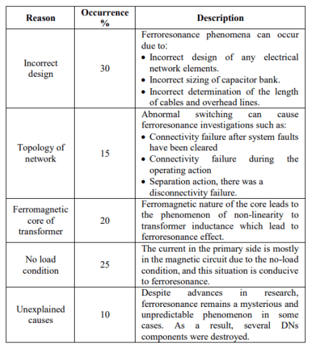
The goal of designing the power system is to deliver electrical power with lowest costs, low pollutant emissions level, maximum efficiency, and high power quality [1]. With the great technological advances these days, devices connected to the electrical grid are becoming more sensitive to system disturbances and transients phenomena such as all events due to switching actions, energizing and de-energizing elements of the power system and faults [2].
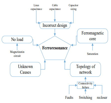
The power system does not always work in a steady-state condition, but it may go via transient states. Despite the short time of transient cases compared to the steady-state conditions of the system, they cause problems such as high voltage or current, poor power quality, drop in voltage or frequency and some harmful phenomena like ferroresonance effect [3]. Hence the interest of researchers are increased to solve these problems to provide the power to the consumer with the appropriate quality. Researchers are working to reduce the problems related to ferroresonance phenomena especially with the increase in nonlinear element in power system [4]. Problems related to transient can be classified into two categories: first impulsive and second oscillatory [5].
Ferroresonance is oscillatory phenomenon threatening the stability of the electrical network [6][7]. Also, ferroresonance refers to voltage displacement or natural instability [8]. It can cause damage to system equipment, insulation and consumer’s distribution devices. Also, it results in misoperation of protection devices due to overvoltage and/or overcurrent of peak value that can exceed more than twice of the normal value [9]–[16]. These phenomenon are caused by abnormal operations results in thermal and electrical stresses [17],[18], [19]. Researchers classified the ferroresonance phenomenon as low frequency electromagnetic transients of frequency ranges from 0.1 Hz to 1 kHz [4], [20]–[22]. This nonlinear phenomena can be blamed for several unexplainable breakdowns [23].
Recently, the phenomenon of ferroresonance has increased significantly in the electrical network. This phenomenon appears in all parts of the electrical network and different voltage levels [19]. Ferroresonance appeared in the protection system elements like Current Transformer (CT) and Potential Transformer (PT). The occurrence of ferroresonance in PT was discussed in [24] and recommendations to avoid the investigation of ferromagnetic resonance were provided. Ref. [25] presented an investigation of the ferroresonance in PT and based on the self-excitation characteristic. PT’s self-excitation characteristic was used to identify ferroresonance. Ref. [26] examined the effects of switching transients and its contribution to the resultant ferroresonance at the coupling Capacitor Voltage Transformer (CVT). Ref. [27] discussed the ferroresonance in PT and infer it through vibration analysis. Ref. [28] explained the extent of the damage caused by the ferroresonance phenomenon on the CVT and proposed a suppression circuit. The occurrence of ferroresonance in PTs during the system energization event was discussed in Ref. [29]. In Ref. [30], the faults in Medium Voltage (MV) network and its role in ferroresonance investigation at Voltage Transformer (VT) were discussed. Ref. [19] presented the occurrence of ferroresonance at the PT terminal on High Voltage (HV) GIS substation. In addition, many studies have shown the occurrence of ferroresonance in PT in different parts of the network, and many solutions and inhibitor circuits have also been presented in Refs. [5], [11], [13], [31]–[35].
In addition, many researchers discussed ferroresonance investigation in the power transformers. Ref. [36] presented the investigation of ferroresonance in power transformer caused by unhealthy switching and introduced its mitigation circuit. Ref. [37] discussed the asymmetrical phases deenergization of the wind farm its role in ferroresonance activation. Ref. [38] presented the prevalence of ferroresonance in the Montazer Qaem 63 kV substation. Ref. [39] provided the initiated of ferroresonance in unloaded power transformer terminated by cable. Ref. [40] explained the effect of power transformer energization in a 400 kV transmission grid on ferroresonance investigation. Ref. [41] dealt with the effect of the variation of Petersen coil on ferroresonance response in a power transformer. Salman in [42] studied the effect of the transmission line outage on ferroresonance response in power transformer. Ref. [18] provided an analytical method to detect the ferroresonance phenomenon in (MV) Networks. In addition, there are many researches in the form of an analysis and a case study only, without presenting actual studies like Refs. [24]- [14].
Ferroresonance also appears in the Distribution System (DS). It’s considered as a critical case because of closeness to loads. Ref. [53] examined the effect of changing the type of distribution transformer on the ferroresonance response, but this study was conducted in a no-load condition. Ref. [54] showed two ferroresonance states investigated in the distribution transformer, but both states were performed when the system was not loaded. Ref. [55] studied the effect of cable length and five legs three-phase distribution transformer on the ferroresonance response. Ref. [56] presented the ferroresonance condition in an underground DS resulting from unhealthy switching cases. Ref. [57] presented three ferroresonance cases in DS integrated with a PV system resulting from the break into interconnection between PV system and the transformer. Ref. [58] presented the occurrence of ferroresonance in DS. It presented the DS in an equivalent circuit without studying a real network.
From the previously presented studies, it is found that the phenomenon of ferroresonance is widespread in all parts of the power system, and a lot of research has been directed to this study. But most of studies dealt with this phenomenon in the form of simple cases or an analytical study only, although this phenomenon is affected by the slightest change in the system. A lot of research that investigated this phenomenon was in protection element parts such as PT and CVT. Others were interested in studying this phenomenon on the power transformer with high and medium voltages. However, the interest in studying this phenomenon in the DS falls short of expectations. Although the DS is the most affected area with loads and any change in these loads can change the network topology and may cause the system to rush into ferroresonance. With the current increase in the use of Distributed Generation (DG) in DSs, its effects on ferroresonance (according to the author’s knowledge) have not been highlighted.
Many studies presented the implementation of DG into DS but, its effect on transit states and ferroresonance investigation still are considered as a research gap. Therefore, this paper focuses on studying the phenomenon of ferroresonance in DSs and the effect of DG penetration on this phenomenon.
This article explains the different factors which caused by the occurrence of ferroresonance and the problems of ferroresonance. The paper provides the physical and analytical methods used to recognize ferroresonance in a network. The different shapes of ferroresonance modes are also explained. Furthermore, the modeling of ferroresonance’s equivalent circuit and transformer response at abnormal switching are provided. The change in transformer response is also displayed as the load varies. The effect of load variation on the radial power system response is studied. The effect of DG implementation on ferroresonance response is presented. Finally, a comparison between methods of mitigating and preventing the ferroresonance is presented. PSCAD/EMTDC software is used in this study.
The rest of the paper is organized as follow. Section II presents ferroresonance phenomena, its definition, the reasons for the occurrence of ferroresonance and ferroresonance problems. Section III presents simulation cases. Section IV presents radial system penetrated with DG as case study. Section V provides the latest mitigation methods of ferroresonance and introduces the implementation of the series ferroresonance suppression circuit. The conclusion of the paper is given in Section IV.
Ferroresonance background
Ferroresonance phenomenon
Ferroresonance means resonance occurred between parameters of the electrical network with element containing ferromagnetic material like a transformer or an inductor [1], [53], [56], [59], [60]. Ferroresonance considered as a special case of resonance [39], [57]. Ferroresonance is unpredictable phenomenon arises due to the interaction between system capacitance and non-linear inductance [45], [61]–[65]. Ferroresonance is a rare non-linear phenomenon in which energy fluctuates between a capacitive element and non-linear inductive element which alternatively becomes saturated. This phenomena causes the system to jump from a stable state to a stationary ferroresonant state [64]. It is still disconcerting phenomena until today [67]. This phenomenon can occur with small changes in the parameters of the network so, it is difficult to be predicted [68], [69]. Investigating ferroresonance is a difficult endeavor, owing to the large number of factors that might influence the phenomenon’s occurrence, as well as the phenomenon’s great sensitivity to very minor changes in power grid parameters [40].
The first to point to this phenomenon is Joseph Bethenod in 1907. He indicated a resonance in the transformer due to non-linear inductance but Paul Boutherot named this phenomena as ferroresonance in 1920 [56], [70]. Ferroresonance differs from normal resonance, or as some researchers call it, linear resonance. Normal resonance is an expected phenomenon that results from an interaction between capacitance and inductance, unlike ferroresonance, which is an unpredictable phenomenon that results from the interaction of capacitance with nonlinear inductance. Table 1 presents a comparison between ferroresonance and linear resonance [1], [53], [57], [71].
Also, Fig. 1 shows the difference between the equivalent resonant and ferroresonance circuits. The ferroresonance circuit incorporate ferromagnetic material resulting in the phenomenon of non-linearity [1], [72]–[76].
Ferroresonance phenomena can occur in all parts of the electrical network and at any level of voltage [72]. There are many causes that lead to ferroresonance effect. The most important reasons are due to incorrect design, topology of network, the ferromagnetic core of transformer and unexplained causes. Table 2 explains these reasons, their percent and their description [48], [77], [78]. These causes are summarized in the illustrated diagram shown in Fig. 2 [40], [48], [51], [79], [80]. Recently, researchers have demonstrated the role of the transformer tank in increasing the ferroresonance effect [81].
Table 1. Comparison between ferroresonance and linear ferroresonance
.
Table 2. Main reasons lead to ferroresonance
.
Fig.1: Comparison between (a) linear resonance and (b) Ferroresonance circuits
Fig.2: Diagram of ferroresonance causes
Ferroresonance Problems
The ferroresonance phenomenon is always accompanied by dangerous problems to power system network. These problems pose a major threat to the continuity and integrity of the power system which represented in the following:
Overvoltage
A ferroresonance in the DS causes a dangerous increase in voltage up to several times the rated value [82]. It is always followed by the occurrence of many other problems in the system such as insulators break down and failure in power system devices which may lead to cut off electrical service [70], [83]–[85].
The problem was displayed in many studies. Ref. [86] introduced the investigation of ferroresonance in an islanding mode of micro grid. The voltage was raised to 8 pu. Ref. [26] introduced the increase of voltage value to 2.5 pu in CCTV. Refs. [87], [41] introduced the increase of voltage value in power transformer to 5 pu and 3 pu as a case study. Ref [88] presented the investigation of overvoltage to 3 pu in VT as an analytical study.
Overcurrent
One of the problems that follows the phenomenon of ferroresonance is the occurrence of a significant increase in current. An increase in the current results in problems such as overheating in parts of the electrical system which lead to damage in system elements and insulators [34], [50].
In [89], the current value in the grid increased to 6 pu. Ref. [90] introduced the increase of current value to 2.5 pu in power transformer. Ref. [21] presented the results of an investigation of overcurrent up to 2 pu into a real system in Slovakia. Ref. [91] introduced the increase of current value to 5.5 pu in VT.
Power distortion
Ferroresonance causes a distortion of the electrical power wave, which results in the occurrence of harmonic problems [82]. These represent a major problem for electronics and sensitive devices. [67], [92]. Fig. 3 explains many shapes of power wave distortion.
Several studies revealed the issue. The distortion in the voltage wave caused by abnormal switching in a PV project connected to the grid was presented in ref. [59]. Refs. [34] and [93] introduced the distortion in VT voltage wave. Ref. [41] provided a case study of a power transformer in ferroresonance and the distortion of its voltage wave.
Saturation for devices containing ferromagnetic material
The fundamental cause of ferroresonance is the nonlinear ferromagnetic characteristics [19]. Ferroresonance causes a saturation of the elements containing ferromagnetic material [94], [95]. High current flow is resulted in saturation, which results in increased heat and irregular vibration of device components [52], [48].
Ref. [96] investigated the role of ferroresonance in transformer saturation. In [65], an analytical study was presented to eliminate saturation that may be caused by ferroresonance with ferromagnetic material. As a case study, Ref. [82] demonstrated the saturation of a nonlinear reactor due to ferroresonance. In [97], an analytical study of a single-phase transformer and the role of ferroresonance in iron core saturation was presented.
Misopertion of protection devices
Significant distortion of the power wave may results in protective device misoperation [98]. The occurrence of ferroresonance results in adverse effects on the voltage transformer, current transformers and measuring apparatuses. All these effects will lead to a defect in the operation of the protection system [25], [26], [30], [67]. Ref. [16] presented the failure of an overcurrent relay (OCR) in the Manitoba grid due to ferroresonance. Ref. [99] introduced challenge to the operation of OCR in DN due to ferroresonance.
Other problems
There are also some other problems that result from the occurrence of ferroresonance, such as the occurrence of abnormal noise, power flickers and damage to some power lines [27], [100], [89]. Ref. [12] presented many problems give rise from ferroresonance such as noise, flicker, damage to electrical equipment and overheating. Despite the complexity of this phenomenon, researchers have tended more recently to find solutions and ways to reduce this phenomenon for protecting the electrical network, its operators and customer devices connected to the network.
Ferroresonance modes and signs
Due to the phenomenon of nonlinearity of the ferroresonance circuit, it has a lot of responses [101]. These responses can be classified into four modes. These modes are known as fundamental mode, sub-harmonic mode, quasi-periodic mode, and chaotic mode [26], [44], [49], [102], [103].
Fundamental Mode
In this mode the current and the voltage have the same period (T) of the system called a period-1 (f0/1 Hz) with the same frequency but contain odd harmonics (3rd, 5th, 7th ,……, nth). It is small in comparison with fundamental component. Fig. 3a shows a Fundamental Ferroresonance (FF) waveform and its frequency spectrum [1], [34], [57], [62], [104].
Sub-Harmonic Mode
In this type, the signals of current and voltage have period multiples of the source period (nT) called a period-n (f0/n Hz) contains fundamental component with (nth) subharmonic. Fig 3b shows a Sub-Harmonic Ferroresonance (SHF) waveform and its frequency spectrum [1], [34], [57], [62], [104].
Quasi-Periodic Mode
This mode is called quasi-periodic mode or subperiodical mode. The signal of current and voltage is not periodic which has non-continuous frequency spectrum. The frequency is represented by equation nf1 + mf2, where f1/f2 are irrational real numbers, and n and m are integers. Fig. 3c shows a quasi-periodic ferroresonance (QF) waveform and its frequency spectrum [1], [34], [57], [62], [104].
Fig.3: Ferroresonance modes
Chaotic Mode
In this mode, the signal of current and voltage is not periodic which has continuous frequency spectrum and any frequency is not cancelled. Fig. 3d shows a Chaotic Ferroresonance (CF) waveform and its frequency [1], [34], [57], [62], [97], [104].
The shape of the system’s response to ferroresonance depends on the parameters of the system and also on the iron core material used with the inductor [44], [105]. Due to the extreme sensitivity of ferroresonance phenomenon, any change in system parameters, at ferroresonance condition, can lead to change in the system behavior [106].
There are several ferroresonance modes as Fig. 3 indicates [48]. Some modes lead to very high voltages and others modes may lead to voltages near nominal values. Therefore, it is important to identify the signs by which this phenomenon could be recognized. It is represented in physical phenomena such as overheat, noise, flicker, surge arrester failure and vibration at power system. When the aforementioned problems appear larger than the allowable limits, it can be a sign of ferroresonance in the system. Table 3 explains these problems and description [48], [53].
In addition the physical signs to identify the presence of ferroresonance are included in Table 3. Also, this phenomena can be recognized through analytical methods such as: Wavelet transform [2], [94], Analysis of the variables in the energy quality factors [38], Short Time Fourier Transform [38], Poincaré maps [92], Bifurcation diagram [95], and Phase plane diagram [38].
Table 3. Summary ferroresonance signs
.
Case study of ferroresonance
To illustrate the ferroresonance phenomenon, case studies are discussed in following subsections. The case studies will focus on ferroresonance in DSs. PSCAD/EMTDC software is used in the study.
Case 1: A capacitor in series with a saturable reactor
The circuit illustrated in Fig. 4a is the equivalent circuit for the ferroresonance phenomenon. The series connection of a capacitance with a saturable reactor and a single phase AC source lead to ferroresonance effect. It is clear that, the voltage has risen considerably beyond the rated value (11 kV) as presented in Fig. 4b. It can be seen the occurrence of quasi-periodic ferroresonance in which the voltage level rises to 3 pu as evidenced.
Fig.4: Ferroresonance of simple circuit
Case 2: A linear inductor with shunt and series capacitors
In this case, the simulation of the circuit is presented in Fig. 5a which consists of linear inductor with shunt capacitor, series capacitor, and 11 kV single phase AC source. Also, the same circuit is implemented in three phase form. It produces a quasi-periodic ferroresonance, as illustrated in Figs. 5a and 5b, with voltages of 3 pu in one phase circuit and 6 pu in three phase circuit.
Fig.5: Ferroresonance overvoltage of case 2 circuit.
Case 3: Abnormal switching of a transformer
In this case, the effect of load variation with abnormal switching of the transformer terminals and its role on ferroresonance occurrence are studied. This study is carried out in four stages: no-load transformer, transformer loaded less than 10%, transformer loaded with 10%, and transformer loaded with more than 10%.
The nature of the load on the terminals of the transformer and the abnormal conditions exposed to them control the shape of the transformer response [95],[111]. Therefore, an abnormal condition like abnormal switching effect on the transformer given at Fig. 6 will studied. This figure presents a 50 MVA, 230/11 kV Unified Magnetic Equivalent Circuit (UMEC) transformer that terminated with load at low voltage side, and three phase source with capacitor at high voltage side. This case presents the effect of the failure of switching off a one phase of the source on transformer with the variation of load. All the abnormal switching actions of all stages are done at 1.5 sec and continue for 4 sec. In the first stage, transformer is not loaded. Failure in disconnecting one phase of the source (two phases separated only) causes ferroresonance on the both sides of the transformer. Figs. 7a and 7b show ferroresonance voltage at transformer high voltage side and low voltage side, respectively.
The voltage on the high voltage side of the transformer increased to 11 pu, while the low voltage side increased to 10 pu, as shown in Fig. 7. This increase in voltage values has harmful effects on the transformer. In this stage chaotic ferroresonance modes are introduced at the both sides of the transformer. It is found that the value of the voltage is increased to a very high values, which results a failure of the equipment definitely.
In the second stage, the transformer is loaded less than 10%. The failed separation of one phase of the source drives the transformer to ferroresonance at both sides with a high value as shown at Fig. 8. The voltage increased to 10 pu on the high voltage side of the transformer and to 10 pu on the low voltage side. Chaotic ferroresonance modes are introduced at the both sides of the transformer.
Fig.6: Equivalent circuit for ferroresonance investigation in transformers
In the third stage, the transformer is loaded with 10% of its rate d value. The failed separation of one phase of the source drives the transformer to chaotic ferroresonance at the both sides. The voltage increased to 3.9 pu on the high voltage side of the transformer and to 3.8 pu on the low voltage side, as shown in Fig. 9.
In the fourth stage, the transformer is loaded more than 10% of its rated value. In the case of unsuccessful separation of one source phases, a temporary transient at switching instant is occurred. On the high voltage side, the voltage value of the healthy phase restores its rated value. The voltage value in the other two phases returns to 0.6 pu and there is no phase difference between the three phases as shown in Fig. 10a. On the low voltage side, the voltage fails as shown in Fig. 10b. There is no ferroresonance effect at this stage.
Fig.7: Transformer ferroresonance voltage wave at no-load
It is concluded from this case studies, to prevent ferroresonance, it is vital to avoid operating the transformers with no load or with light loads. According to Ref. [57], the transformer must loaded at least with 10% of its capacity to prevent ferroresonance investigation but, in the third stage, when the transformer is loaded with 10% of its capacity and an abnormal switching is implemented, the ferroresonance appears. Therefore, it is preferable to load transformers more than 10% of their capacity.
Fig.8: Tranformator ferroresonance voltage wave at load less 10%
Fig.9: Transformer ferroresonance voltage wave at 10% load
Fig. 10: Transformer ferroresonance voltage at load more than 10%
Study of ferroresonance in radial distribution DG
The DSs are usually planned as a loop topology to improve system performance and increase system reliability. However, some limits may require the use of the Radial Distribution System (RDS).
In this section, two case studies are presented. The first is the investigation of ferroresonance in 13.2 kV RDS. The second is the investigation of ferroresonance in the 13.2 kV RDS integrated with DG unit. The distribution is feeding from 230 kV overhead transmission line coming from generation plant as shown in Fig. 10a [112].
The system is lightly loaded, so the current values are insignificant. Despite the presence of ferroresonance, the current did not surpass the rated values. As a result, the focus of the research was on voltage values.
In the first case study, a light load is connected at the distribution transformer terminal. The system is normal, however, if one sending end conductor of the transmission line are being disconnected, the voltage fluctuated with a high value on both sides of the transformer. The capacitance of the transmission line interacts with the inductance of the distribution transformer. It results in ferroresonance as shown in Figs. 11b and 11c. Figs. 11b and 11c present the chaotic ferroresonance mode on both sides of the transformer at the moment of one of the transmission line conductors is cut. It is obvious that, the value of voltage rises more than 4 pu in the high voltage side and 2.7 pu in the low voltage side.
Fig.11: Ferroresonance in radial system integrated with DG
With the variation of load value, the increase of the load results in the disappearance of ferroresonance phenomenon even if one of the transmission line conductors is disconnected.
In the second case, the radial DS is penetrated with a DG unit. The 16 kV DG unit is connected to the distribution zone through 16/13.2 kV, 30 MVA, transformer. The described system is shown in Fig. 12a. With the penetration of DG into the system, the ferroresonance phenomenon is disappeared, even if one of the transmission line conductors or more are disconnected at any load value. In this case, the introduction of DG resulted in ferroresonance mitigation by altering the system topology. By studying all abnormal separation on DG and the transmission line, the ferroresonance was investigated only in the case of the separation of DG with the breakdown of phase A of the transmission line. Chaotic ferroresonance was investigated. It is found that the voltage value was increased on the low voltage side for 2.3 pu and for 4 pu on the high voltage side and 2.8 pu on the DG side as shown in Figs.12b and 12c.
All separation events implemented at the time 0.3 sec and the study conducted for one sec. The voltage levels resulted from ferroresonance phenomenon are extremely high. The abnormal switching action and the unexpected conductor failure may cause harmful damage to the power system parts. As a result, it’s critical to eliminate the factors that generate ferroresonance, such as loading nonlinear inductive elements with light or no load and failing to defend against phase failure.
Therefore, it is important to provide system with protection against phase failure. Incorporating DG into the radial DS can reduce the incidence of ferroresonance, but may result in worse ferroresonance in some cases. So, the researchers must guide their efforts for optimizing the use of DG and avoiding ferroresonance.
Fig. 12: Ferroresonance in radial system integrated with DG
Mitigation of ferroresonance
Review of mitigation methods
Ferroresonance causes a significant increase in voltage and/or current, and this is considered a great threat to the parts of the electrical network from damage. Therefore, the researchers focused on reducing the occurrence of this phenomenon to avoid its major technical and economic problems.
Prevention of ferroresonance is divided into two ways. The first is protection methods provided for the electrical network to protect and reduce the bad effects of this phenomenon [113]. The second is the precautions taken to prevent the occurrence of ferroresonance into the electrical network.
Ferroresonance prevention methods, are all the methods and precautions taken by the electrical network operator to prevent the occurance of ferroresonance in the power system. Table 4 shows the most important precautions taken used to prevent ferroresonance. Ferroresonance mitigation techniques are all the techniques used to restrain the high values of voltage and current resulting from the ferroresonance [58]. Table 5 summarized the most important methods used to mitigate and its method of study.
Generally, Ferroresonance Suppression Circuits (FSC) are classified into three categories [33]. First, active FSC which consist of resonance circuit and operate with high impedance in normal frequency and low impedance in abnormal frequency to connect suppression element [26]. Second, passive FSC which contain of saturable reactor that saturate when the voltage value passed 1.5 pu then its impedance is reduced and connecting damping resistor [26]. Third, power electronics FSC which consist of two power electronic switches used to damp overvoltage during ferroresonance, and provide a resistive channel to ground [33].
Ref. [114] presented the using of resistor with two oneway controllable switches connected back to back implemented on the secondary side of the PT as a damping resistor to suppress ferroresonance. Ref. [115] presented the implementation of damping resistor connected with secondary winding of the transformer as suppress ferroresonance. Ref. [116] relied on the use of a resistance with an electronic switches implemented on PT secondary side to reduce the ferroresonance, but presented a different control circuit for the switches. It presented the control of the conduction of this resistance by a mechanical switch or a saturable reactor, having a saturation voltage. The saturation voltage is higher than the rated secondary voltage of the transformer but still quite near to it. The saturable reactor is saturated when ferroresonance occurs and the resistance can damp ferroresonance. Also, Ref. [117] used a parallel reactor with the secondary side of the PT for mitigating ferroresonance. Ref. [118] introduced the use of thyristor driven spontaneous close shunt reactors as a solution to ferroresonance on a power transmission line which reduces the duration of the high voltage result from ferroresonance.
A gas discharge lamp was used in [32] as a memristor emulator connected to the secondary of the CVT to minimise the ferroresonance. Ref. [119] introduced ferroresonance limiter consists of damping resistor resulted in eliminate of chaotic ferroresonance oscillations started with series capacitors controlled by thyristor in the CVT.
Ref. [120] introduced the design of two ferroresonance suppression circuit implemented on the step down side of the CVT. The first is to use a resistance only, and the second is to use RLC circuit. Refs. [71] and [109] recommended the implementation of damping resistor or air core reactor bank connected with transformer secondary winding as ferroresonance mitigation techniques. Refs. [110] and [111] presented the design of converter acted as damping resistor emulators to mitigate ferroresonance oscillation. Ref. [124] presented smart ferroresonance limiter circuit that consist of four magnetically coupled windings. The primary winding and the PT are linked in parallel. The secondary winding is utilised to reduce ferroresonance overvoltage value. The third and fourth windings are employed to detect ferroresonance beginning in the positive and negative half cycles of the transient overvoltage, sequentially.
Ref. [98] recommended the installation of overvoltage protection element at suitable locations to eliminate overvoltage generation from ferroresonance. Ref. [42] presented the using of Static Var Compensator (SVC) to mitigate ferroresonance by network voltage and reactive power control. Ref. [99] introduced the use of intelligent overcurrent protection, based on wavelet and neural network, to distinguish ferroresonance from transients cases. Ref. [127] presented a ferroresonance limiter, which consisted of anti-parallel IGBTs connected with series resonant LC. Fault current limiters with an inductive shielded core presented in [87] as a method to mitigate power transformers with chaotic ferroresonance.
Ref. [113] presented several ways to reduce the impact of ferroresonance, namely: connect nonlinear resistance to the high voltage side’s neutral point, install eliminating resistance to the secondary side of the transformer and grounding the neutral point via arc suppression coil. Ref. [128] presented the connection of metal oxide varistor to the secondary winding ofthe transformer as a means of limiting ferroresonance. Ref. [129] presented the inserting an air gap in the magnetic path of the voltage transformer core which resulting in the linearization of the magnetizing characteristic and lowering the risk of ferroresonance.
Ref. [107] introduced method to mitigate ferroresonance by adding damping reactor which is integrated with ferroresonance detection and suppression device to absorb the energy produced by ferroresonance. The opening of the opposite end of the line/transformer to de-energize the circuit breaker, before opening it, is presented in Ref. [130] as a solution to mitigate ferroresonance. Ref. [131] presented the use of ferroresonance eliminator consisted of resistance located at the three-phase PT’s primary side’s neutral point. Ref. [41] introduced grounding the power transformer by Petersen coil to mitigate ferroresonance. Ref. [132] presented three ferroresonance mitigation methods represented in grounding the PT primary side of nonlinear resistance, connecting a damping resistor in open delta winding of PT or choosing PT with best excitation characteristics. It turns out that the effect of DG on ferroresonance has not been thoroughly investigated and remains as a gap point. It was unclear how suppression ferroresonance methods would be implemented with the DGs. Furthermore, the effect of ferroresonance and DG on the DSs was not clarified, and researchers did not pay enough attention to solutions to this problem in the DSs.
Implementation of series ferroresonance suppression circuit
The Tuned LC Circuit (TLCC) was implemented by connecting a capacitor and an inductor in series and adjusting their values in resonance state according to Eq. (1) to have a negligible impedance at the system’s steady-state frequency [127]. TLCC impedance reduced the amplitude of overvoltage to an acceptable level under abnormal conditions. In this study, TLCC will be tested in both radial system and radial system integrated with DG that given in section IV. In the normal state, TLCC circuit did not cause a voltage drop, and in the abnormal condition, it mitigates the overvoltage value in both cases as given in the following paragraphs.
.
Table 4. Ferroresonance preventing methods
Table 5. Ferroresonance mitigating techniques
.
.
Table 6. Voltage of radial system with and without DG
.
Table 7. Voltage of radial system integrated with DG with and without TLCC
.
TLCC is implemented on the low voltage side of the transformer at the RDS described in section IV resulted in ferroresonance mitigation
The value of the voltage is reduced as presented in Table 6. TLCC results in suppression of the ferroresonance after 0.08 sec from the separation. TLCC’s efficiency in decreasing the overvoltage value is demonstrated in Fig. 13.
Applying TLCC with the radial system integrated with DG results in ferroresonance mitigation. The TLCC is implemented on the DG side of the distribution transformer. It results in decreasing the overvoltage values presented in Table 7. TLCC’s efficiency in decreasing the overvoltage value is demonstrated in Fig. 14.
Fig.13: Voltage waveform with and without implementation of TLCC in radial distribution system
Fig.14: Voltage waveform with and without implementation of TLCC in radial distribution system integrated with DG
Conclusion
In this paper, a state of art of ferroresonance and the most obvious signs of ferroresonance, as well as the analytical methods used to detect it, are presented. This phenomenon is verified by simulating its equivalent circuit using PSCAD/EMTDC software. The investigation of ferroresonance in power transformers and the effect of changing the load on the phenomenon are verified. It is concluded from transformer study that it is preferable to load transformers at more than 10% of their capacity to avoid ferroresonance.
This paper also studies the penetration of the DG into the radial system and the extent of its impact on the occurrence or prevention of ferroresonance as a case study. Results showed that the penetration of DGs into the distribution zone has an active role in mitigating the investigation of ferroresonance. The ferroresonance is appeared only during disconnecting the DG and a phase of the transmission line with keeping the DG transformer connected to the distribution side. The rate of ferroresonance occurrence in the case of DG integration is lower than that occurs in the case of DG unintegrated distribution system due to the need for separating more than one position at the same time.
Finally the analytical methods used to prevent this phenomena are presented and compared. Also the TLCC method was implemented to suppress ferroresonance. The results proved that the system penetrated with DG responds faster to TLCC ferroresonance mitigation method more than the distribution system without DG.
REFERRENCES
[1] S. P. Ang, Ferroresonance simulation studies of transmission systems, PHD, Faculty of Engineering and Physical Sciences. Manchester: the university of manchester, 2010. [2] S. Poomima and C. P. Sugumaran, “Identification of ferroresonance phenomena using wavelet transforms,” in 2016 International Conference on Control, Instrumentation, Communication and Computational Technologies (ICCICCT), 2016, pp. 126–131. [3] V. Arun kumar, S. Elango, M. Prabu, B. Ramraj, “Transient Overvoltages And Its Prevention And Protection,” ” International Journal of Engineering Trends and Technology., vol. 68, no. 3, pp. 22–25, 2020. [4] A. Akinrinde, A. Swanson, and R. Tiako, “Investigation of Temporary Overvoltage on Microgrid with Emphasis on Ferroresonance,” Int. J. Eng. Res. Africa, vol. 39, pp. 32–46, 2018, [5] P. H. B. de S. Pinheiro, M. L. C. Vidal, F. F. da Rocha, B. W. França, and M. Z. Fortes, “Ferroresonance evaluation on capacitor voltage transformers,” Electr. Eng., vol. 102, no. 3, pp. 1775–1783, 2020, [6] V. Valverde, J. Mazón, G. Buigues, and I. Zamora, “Ferroresonance suppression in voltage transformers,” Prz. Elektrotechniczny, vol. 88, no. 1 A, pp. 137–140, 2012. [7] M.Yang, W. Sima, P. Duan, M. Zou, D. Peng, Q. Yang, Q. Duan,, “Electromagnetic transient study on flexible control processes of ferroresonance,” Int. J. Electr. Power Energy Syst., vol. 93, pp. 194–203, 2017. [8] S. J. Kruger and J. A. de Kock, “Ferroresonance: A Review of the Phenomenon and Its Effects,” 2021 Southern African Universities Power Engineering Conference/Robotics and Mechatronics/Pattern Recognition Association of South Africa, 2021, pp. 1–6. [9] S. Hassan, M. Vaziri, and S. Vadhva, “Review of ferroresonance in power distribution grids,” 2011 IEEE International Conference on Information Reuse Integration, 2011, pp. 444–448. [10] L. V Bykovskaya and V. Bykovskiyi, “Simulation of a Voltage Transformer with a Magnetic Core Made of Amorphous Steels,” 2020 International Conference on Industrial Engineering, Applications and Manufacturing (ICIEAM), 2020, pp. 1–5. [11] L. Zhao, X. Chen, L. Ye, Y. Yang, S. Wang, and B. Yu, “Research on Ferroresonance of Electromagnetic Voltage Transformer in 550kV HGIS,” 2019 IEEE 3rd International Conference on Circuits, Systems and Devices (ICCSD), 2019, pp. 34–38. [12] V. Valverde, G. Buigues, A. Mazon, I. Zamora, and I. Albizu, “Ferroresonant Configurations in Power Systems,” Renew. energy power Qual. J., pp. 474–479, 2012. [13] M. Xu and L. Zhu, “Ferro-resonance Overvoltage Identification Using Earth Capacitance and Excitation Inductance of Ratio Method,” 2017 International Conference on Advances in Materials, Machinery, Electrical Engineering (AMMEE), 2017, pp. 335–359. [14] M. Mikhak-Beyranvand, B. Rezaeealam, J. Faiz, and A. Rezaei-Zare, “Impacts of ferroresonance and inrush current forces on transformer windings,” IET Electr. Power Appl., vol.13, no. 7, pp. 914–921, 2019. [15] S. Rezaei, “Prevention of False Operation of Distance Relay in Ferroresonance,” Int. J. Adv. Res. Electr. Electron. Instrum. Eng., vol. 5, 2016. [16] S. Rezaei, “Impact of Ferroresonance on protective relays in Manitoba Hydro 230 kV electrical network,” 2015 IEEE 15th International Conference on Environment and Electrical Engineering (EEEIC), 2015, pp. 1694–1699. [17] N. Yang, Y. Han, C. Wu, R. Jia, and C. Liu, “Dynamic analysis and fractional-order adaptive sliding mode control for a novel fractional-order ferroresonance system,” Chinese Phys. B, vol.26, no. 8, p. 80503, 2017, [18] K. Solak, W. Rebizant, and M. Kereit, “Detection of Ferroresonance Oscillations in Medium Voltage Networks,” Energies, vol. 13, no. 16, p. 4129, 2020, [19] D. Zhang, X. Hu, H. Zhang, H. Yu, and Y. Shen, “Ferroresonance Analysis of 500kV GIS Substation during Commissioning Process,” IOP Conf. Ser. Earth Environ. Sci., vol. 514, p. 42042, 2020, [20] W. Sima, M. Zou, M. Yang, D. Peng, and Y. Liu, “Saturable reactor hysteresis model based on Jiles–Atherton formulation for ferroresonance studies,” Int. J. Electr. Power Energy Syst., vol. 101, pp. 482–490, 2018, [21] M. Kanálik, A. Margitová, B. Dolník, D. Medveď, M. Pavlík, and J. Zbojovský, “Analysis of low-frequency oscillations of electrical quantities during a real black-start test in Slovakia,” Int. J. Electr. Power Energy Syst., vol. 124, p. 106370, 2021, [22] E. O. Egorova, “development of the coil volume method for time-domain simulation of internal faults in transformers,” PHD Thesis, michigan technological university, 2019. [23] S.E. Zirka, Y.I. Moroz, A.V. Zhuykov, D.A. Matveev, M.A. Kubatkin, M.V. Frolov, M. Popov, Eliminating VT uncertainties in modeling ferroresonance phenomena caused by single phase-to-ground faults in isolated neutral network,” Int. J. Electr. Power Energy Syst., vol. 133, no. May, p. 107275, 2021. [24] L. Zhen, C. JianBin, X. Yuan, X. Zhen, W. Shenhua, and W. Tian, “The ferroresonance of 10kV distribution PT during live working operation,” The 16th IET International Conference on AC and DC Power Transmission (ACDC), 2021, pp. 1641–1646. [25] Y. Zhang, S. Xie, N. Jiang, Z. Zhao, D. Luo, N. Wang and J. Li “Analysis of Pt Ferroresonance based on Excitation Characteristic and Self-Excitation Mechanism,” J. Phys. Conf. Ser., vol. 1732, p. 012180, 2021. [26] M. Tajdinian, M. Allahbakhshi, S. Biswal, O. P. Malik, and D. Behi, “Study of the Impact of Switching Transient Overvoltages on Ferroresonance of CCVT in Series and Shunt Compensated Power Systems,” IEEE Trans. Ind. Informatics, vol. 16, no. 8, pp. 5032–5041, 2020. [27] A. Arroyo, R. Martinez, M. Manana, A. Pigazo, and R. Minguez, “Detection of ferroresonance occurrence in inductive voltage transformers through vibration analysis,” Int. J. Electr. Power Energy Syst., vol. 106, pp. 294–300, 2019. [28] P. Sridharan and P. S. C, “Memristor emulator – a nonlinear load for reduction of ferroresonance in a single-phase transformer,” Circuit World, vol. 47, no. 1, pp. 87–96, 2020. [29] I. R. Pordanjani, X. Liang, Y. Wang, and A. Schneider, “Single-Phase Ferroresonance in an Ungrounded System during System Energization,” IEEE Trans. Ind. Appl., vol. 7, no. c, 2021. [30] K. Solak and W. Rebiant, “Modeling of Ferroresonance Phenomena in MV Networks,” in 2018 IEEE Electrical Power and Energy Conference (EPEC), 2018, pp. 1–6. [31] A. Heidary, K. Rouzbehi, H. Radmanesh, and J. Pou, “Voltage Transformer Ferroresonance: An Inhibitor Device,” IEEE Trans. Power Deliv., vol. 35, no. 6, pp. 2731-2733, 2020. [32] V. Mohan, S. Poornima, and C. P. Sugumaran, “Mitigation of Ferroresonance in Capacitive Voltage Transformer Using Memelements,” 2019 International Conference on High Voltage Engineering and Technology (ICHVET), 2019, pp. 1–5. [33] M. Tajdinian, M. Allahbakhshi, B. Behdani, D. Behi, and A. Goodarzi, “Probabilistic framework for vulnerability analysis of coupling capacitor voltage transformer to ferroresonance phenomenon,” IET Sci. Meas. Technol., vol. 14, no. 3, pp. 344–351, 2020. [34] I. G. Ngurah Satriyadi Hernanda, I. M. Yulistya Negara, D. A. Asfani, D. Fahmi, M. R. Ramadhan, and B. K. Yegar Sahaduta, “Study of Ferroresonance in 150 kV High Voltage Inductive Voltage Transformer,” in 2020 International Seminar on Intelligent Technology and Its Applications (ISITIA), 2020, pp. 386–391. [35] M. Tajdinian, M. Allahbakhshi, S. Biswal, O. P. Malik, and D. Behi, “Study of the Impact of Switching Transient Overvoltages on Ferroresonance of CCVT in Series and Shunt Compensated Power Systems,” IEEE Trans. Ind. Informatics, vol. 16, no. 8, pp. 5032–5041, 2020. [36] E. A. Badran, M. E. M. Rizk, and M. H. Abdel-Rahman, “Investigation of ferroresonance in offshore wind farms.,” J. Am. Sci., vol. 7, no. 9, pp. 941–950, 2011. [37] W. Farm, A. Akinrinde, and A. Swanson, “Investigation and Mitigation of Temporary Overvoltage Caused by DeEnergization on an,” 2020. [38] S. Aref, A. S. Anaraki, and D. A. Zarchi, “Probability Evaluation of Occurrence of Ferroresonance in Montazer Qaem 63kV Substation,” 2020 14th International Conference on Protection and Automation of Power Systems (IPAPS), 2019, pp. 7–13. [39] A. Nassar, A.-M. Taalab, M. Izzularab, and N. Elkalashy, “Investigation of Resonance and Ferroresonance Overvoltages due to Cable-Transformer Interactions,” ERJ. Eng. Res. J., vol. 43, no. 4, pp. 261–271, 2020. [40] M. Polewaczyk, S. Robak, and M. Szewczyk, “Investigation on ferroresonance due to power transformer energization in high voltage 400 kV transmission grid,” Arch. Electr. Eng., vol. 68, no. 4, pp. 771–786, 2019. [41] I. G. Ngurah Satriyadi Hernanda, I. M. Yulistya Negara, D. A. Asfani, D. Fahmi, M. Wahyudi, and K. S. Anugrah, “Study of Petersen Coil Grounding System Inductance Variation on Ferroresonance in 150 kV Transformer,” in 2018 International Seminar on Intelligent Technology and Its Applications (ISITIA), 2018, pp. 141–146. [42] S. Rezaei, “Impact of transmission line and plant outage on ferroresonance in AC transmission system and new suppression method,” in 13th IET International Conference on AC and DC Power Transmission (ACDC 2017), 2017, pp. 1–6. [43] M. Yang, W. Sima, Q. Yang, J. Li, M. Zou, and Q. Duan, “Nonlinear characteristic quantity extraction of ferroresonance overvoltage time series,” IET Gener. Transm. Distrib., vol. 11, no. 6, pp. 1427–1433, 2017. [44] I. M. Yulistya Negara, I. G. Ngurah Satriyadi Hernanda, D. A. Asfani, D. Fahmi, M. Wahyudi, and R. Hidayat, “Comparison of Ferroresonance Response on Three Phases Transformer with Different Core Material: M5 and ZDKH,” 2018 International Seminar on Intelligent Technology and Its Applications (ISITIA), 2018, pp. 129–134. [45] M. Zou, “Accurate simulation model for a three-phase ferroresonant circuit in EMTP–ATP,” Int. J. Electr. Power Energy Syst., vol. 107, pp. 68–77, 2019. [46] R. S. Pal and M. Roy, “Study and Verification of Ferroresonance Simulated with Rudenburg’s Method,” in 2021 Innovations in Energy Management and Renewable Resources(52042), 2021, pp. 1–5. [47] D. K. Buslaev, J. K. Ochkovskaya, and L. D. Ziles, “Ferroresonance occurrence conditions in a simple nonlinear circuit,” Proc. 3rd 2021 Int. Youth Conf. Radio Electron. Electr. Power Eng. REEPE 2021, pp. 2–6, 2021. [48] S. Boutora and H. Bentarzi, “Ferroresonance Study Using False Trip Root Cause Analysis,” Energy Procedia, vol. 162, pp. 306–314, 2019. [49] M. S. H. Bini, S. P. Ang, K. S. K. Yeo, A. Khalil, and S. Jaafar, “Analytical prediction of initiation of ferroresonance modes,” J. Phys. Conf. Ser., vol. 1529, p. 32087, 2020, [50] I. M. Y. Negara, D. A. Asfani, I. G. N. S. Hernanda, D. Fahmi, Verdiansyah, and B. K. Aji, “Wavelet Transformation Selection for Detection of Ferroresonance Behaviour,” in 2019 International Seminar on Intelligent Technology and Its Applications (ISITIA), 2019, pp. 253–258. [51] M. Sowa and Ł. Majka, “Ferromagnetic core coil hysteresis modeling using fractional derivatives,” Nonlinear Dyn., vol. 101, no. 2, pp. 775–793, 2020. [52] M. Mikhak-Beyranvand, J. Faiz, A. Rezaei-Zare, and B. Rezaeealam, “Electromagnetic and thermal behavior of a single-phase transformer during Ferroresonance considering hysteresis model of core,” Int. J. Electr. Power Energy Syst., vol. 121, p. 106078, 2020. [53] M. Hajizadeh, I. Safinejad, and N. Amirshekari, “Study and comparison of the effect of conventional, low losses and amorphous transformers on the ferroresonance occurrence in electric distribution networks,” CIRED – Open Access Proc. J., vol. 2017, no. 1, pp. 865–869, 2017. [54] M. I. Mosaad and N. A. Sabiha, “Ferroresonance Overvoltage Mitigation using STATCOM for Grid-Connected Wind Energy Conversion Systems,” J. Mod. Power Syst. Clean Energy, pp.1–9, 2021. [55] A. I. Abdi, J. J. Walker, and J. S. Djeumen, “The Effect Of Cable Length On Ferroresonance In Low-Loss Distribution Transformers,” in 2021 Southern African Universities Power Engineering Conference/Robotics and Mechatronics/Pattern Recognition Association of South Africa (SAUPEC/RobMech/PRASA), 2021, pp. 1–4. [56] S. O. Koledowo, E. C. Ashigwuike, and A. Bawa, “A study of ferroresonance in underground distribution network for 15MVA, 33/11 kV injection substation,” Niger. J. Technol., vol.39, pp. 219–227, 2020. [57] N. Thanomsat, B. Plangklang, and H. Ohgaki, “Analysis of Ferroresonance Phenomenon in 22 kV Distribution System with a Photovoltaic Source by PSCAD/EMTDC,” Energies, vol. 11, p. 1742, 2018. [58] A. B. Nassif, M. Dong, S. Kumar, and G. Vanderstar, “Managing Ferroresonance Overvoltages in Distribution Systems,” in 2019 IEEE Canadian Conference of Electrical and Computer Engineering (CCECE), 2019, pp. 1–4. [59] A. Abdullah, “A Ferroresonance Study of a 240 MW Solar PV Project,” 2018 IEEE Industry Applications Society Annual Meeting (IAS), 2018, pp. 1-4. [60] S. P. Ang, J. Peng, and Z. Wang, “Identification of key circuit parameters for the initiation of ferroresonance in a 400-kV transmission system,” 2010 International Conference on High Voltage Engineering and Application, 2010, pp. 73–76. [61] B. Behdani, M. Allahbakhshi, and M. Tajdinian, “On the impact of geomagnetically induced currents in driving series capacitor compensated power systems to ferroresonance,” Int. J. Electr. Power Energy Syst., vol. 125, p. 106424, 2021. [62] L. Chen, J. Wang, W. Sima, and T. Yuan, “Classification of Fundamental Ferroresonance, Single Phase-to-Ground and Wire Breakage Over-Voltages in Isolated Neutral Networks,” Energies, vol. 4, no. 9, pp. 1301–1320, 2011. [63] Ł. Majka, “Fractional Derivative Approach in Modeling of a Nonlinear Coil for Ferroresonance Analyses,” in Non-Integer Order Calculus and its Applications, 2019, pp. 135–147. [64] M. Navaei, A. A. Abdoos, and M. Shahabi, “A new control unit for electronic ferroresonance suppression circuit in capacitor voltage transformers,” Int. J. Electr. Power Energy Syst., vol.99, pp. 281–289, 2018. [65] I. M. Bedritskiy and K. K. Jurayeva, “Estimation of Errors in Calculations of Coils with Ferromagnetic Core,” in 2020 International Conference on Industrial Engineering, Applications and Manufacturing (ICIEAM), 2020, pp. 1–6. [66] M. Kutija and L. Pravica, “Effect of harmonics on ferroresonance in low voltage power factor correction system—A case study,” Appl. Sci., vol. 11, no. 10, 2021. [67] M. Wahyudi, I. M. Yulistya Negara, D. Anton Asfani, I. G. N. S. Hernanda, and D. Fahmi, “Investigation of Ferroresonance Physical Behaviours on Three Phases Transformer with Unsymmetrical Core Leg,” in 2018 International Seminar on Application for Technology of Information and Communication, 2018, pp. 66–70. [68] J. Wisniewski, E. Anderson, and J. Karolak, “Search for network parameters preventing ferroresonance occurrence,” in 2007 9th International Conference on Electrical Power Quality and Utilisation, 2007, pp. 1–6. [69] M. Esmaeili, M. Rostami, G. B. Gharehpetian, and C. P. McInnis, “Ferroresonance After Islanding of Synchronous Machine-Based Distributed Generation,” Can. J. Electr. Comput. Eng., vol. 38, no. 2, pp. 154–161, 2015. [70] F. In and P. Systems, 13 – Ferroresonance in power systems energiforskrapport-2017-457. Report, 2017. [71] S. Chen and H. Yu, “A Review on Overvoltages in Microgrid,” in 2010 Asia-Pacific Power and Energy Engineering Conference, 2010, pp. 1–4. [72] R. Zhang, H. Li, S. P. Ang, and Z. Wang, “Complexity of ferroresonance phenomena: sensitivity studies from a singlephase system to three-phase reality,” in 2010 International Conference on High Voltage Engineering and Application, 2010, pp. 172–175. [73] B. Baldwin, S. S. Sabade, and S. Joshi, “A Study of Ferroresonance & Mitigation Techniques April,” michigan university, 2013. [74] K. Milicevic, E. K. Nyarko, and I. Biondic, “Chua’s model of nonlinear coil in a ferroresonant circuit obtained using Dommel’s method and grey box modelling approach,” Nonlinear Dyn., vol. 86, no. 1, pp. 51–63, 2016. [75] N. Thanomsat and B. Plangklang, “Ferroresonance phenomenon in PV system at LV side of three phase power transformer using of PSCAD simulation,” 2016 13th International Conference on Electrical Engineering/Electronics, Computer, Telecommunications and Information Technology (ECTI-CON), 2016, pp. 1-4. [76] A. Akinrinde, A. Swanson, and R. Tiako, “Dynamic Behavior of Wind Turbine Generator Configurations during Ferroresonant Conditions,” Energies, vol. 12, p. 639, 2019. [77] F. Ben Amar and R. Dhifaoui, “Analytical Approach for the Systematic Research of the Periodic Ferroresonant Solutions in the Power Networks,” Energy Power Eng., vol. 03, pp. 450–477, 2011, [78] L. Jiaxin, L. Xuchen, W. Yanan, W. Defu, and T. Jianeng, “Discriminate Method of Power Frequency Ferroresonance in System with Non-Effectively Earthed Neutral of Three-Phase Enclosed GIS,” in 2018 China International Conference on Electricity Distribution (CICED), 2018, pp. 801–805. [79] T. Şengüler and S. Şeker, “Continuous wavelet transform for ferroresonance detection in power systems,” Electr. Eng., vol. 99, no. 2, pp. 595–600, 2017, [80] A. Karrar, M. Ahmed, A. Ali, S. Mohammed, R. Hay, and R. Johnson, “Investigation of Ferroresonance Incidents in the EPB Distribution Network,” 2018. [81] Q. Wu, D. Deswal, M. Yang, S. Wang, and F. de León, “Experimental Study of Magnetic Effects of Steel Tanks on Three-Phase Transformer Transients,” IEEE Trans. Power Deliv., vol. 35, no. 2, pp. 665–673, 2020. [82] Ł. Majka and M. Klimas, “Diagnostic approach in assessment of a ferroresonant circuit,” Electr. Eng., vol. 101, no. 1, pp.149–164, 2019. [83] R. Cetina, V. Torres, and M. Madrigal, “Simulations of ferroresonance in transformers using ATP (Alternative Transient Program),” in 2018 IEEE International Autumn Meeting on Power, Electronics and Computing (ROPEC), 2018, pp. 1–7. [84] R. El Mahayni, A. Gheeth, J. Thomai, and R. Sudhir, “Ferroresonance measurements and modeling; a waveform is worth a thousand words,” in 2018 Petroleum and Chemical Industry Conference Europe (PCIC Europe), 2018, pp. 1–10. [85] A. H. Abu Bakar, S. A. Khan, T. Kwang, and N. Abd Rahim, “A Review of Ferroresonance in Capacitive Voltage Transformer,” IEEJ Trans. Electr. Electron. Eng., vol. 10, 2015, [86] V. George, G. K. Kumaran, J. Shivashankari, and S. Ashok, “Analysis of ferroresonance in a hybrid micro-grid with multiple distributed resources,” in 2016 International Conference on Electrical, Electronics, and Optimization Techniques (ICEEOT), 2016, pp. 1286–1291. [87] H. Fordoei and S. A. Afsari, “Elimination of chaotic ferroresonance in power transformer by ISFCL,” Int. J. Electr. Power Energy Syst., vol. 68, 2015. [88] S. Emiroglu, Y. Uyaroglu, and T. E. Gümüş, “Recursive backstepping control of ferroresonant chaotic oscillations consisting between grading capacitor with nonlinear inductance of voltage transformer,” Eur. Phys. J. Spec. Top., vol. 230, no. 7, pp. 1829–1837, 2021. [89] A. Heidary, H. Radmanesh, A. Bakhshi, S. Samandarpour, K. Rouzbehi, and N. Shariati, “Compound ferroresonance overvoltage and fault current limiter for power system protection,” IET Energy Syst. Integr., vol. 2, no. 4, pp. 325–330, 2020. [90] S Poornima, “Suppression of ferroresonance using passive memristor emulator” , Chin. Phys. Vol. 30, no. 6, P.068401,2021. [91] Z. Abdul-Malek, K. Mehranzamir, B. Salimi, H. Nabipour Afrouzi, and S. Vahabi Mashak, “Investigation of ferroresonance mitigation techniques in voltage transformer using ATP-EMTP simulation,” J. Teknol. (Sciences Eng., vol. 64, no. 4, pp. 85–95, 2013, [92] S. Rezaei, “Power Oscillation Due to Ferroresonance and Subsynchronous Resonance,” Power System Stability, Kenneth Eloghene Okedu, IntechOpen, 2019. [93] V. Valverde, A. J. Mazón, I. Zamora, and G. Buigues, “Ferroresonance in voltage transformers: Analysis and simulations,” Renew. Energy Power Qual. J., vol. 1, no. 5, pp. 465–471, 2007, [94] M. Akbari, A. Rezaei-Zare, M. A. M. Cheema, and T. Kalicki, “Air gap inductance calculation for transformer transient model,” IEEE Trans. Power Deliv., vol. 36, no. 1, pp. 492–494, 2021. [95] A. Tokić, M. Kasumović, M. Pejić, V. Milardić, and T. Cetin Akinci, “Determination of single-phase transformer saturation characteristic by using Nelder–Mead optimization method,” Electr. Eng., 2021. [96] R. Perez Pineda, R. Rodrigues, and A. Aguila Tellez, “Analysis and Simulation of Ferroresonance in Power Transformers using Simulink,” IEEE Lat. Am. Trans., vol. 16, no. 2, pp. 460–466, 2018. [97] J. A. Corea-Araujo, J. A. Martinez-Velasco, F. GonzálezMolina, J. A. Barrado-Rodrigo, L. Guasch-Pesquer, and F. Castro-Aranda, “Validation of single-phase transformer model for ferroresonance analysis,” Electr. Eng., vol. 100, no. 3, pp. 1339–1349, 2018. [98] R. Minkner and J. Schmid, “Voltage Measurement,” in The Technology of Instrument Transformers : Current and Voltage Measurement and Insulation Systems, Wiesbaden: Springer Fachmedien Wiesbaden, 2022, pp. 139–233. [99] S. Rezaei, “Intelligent overcurrent protection during Ferroresonance in smart distribution grid,” in 2019 IEEE International Conference on Environment and Electrical Engineering and 2019 IEEE Industrial and Commercial Power Systems Europe (EEEIC / I&CPS Europe), 2019, pp. 1–6. [100] O. Akgün, T. C. Akinci, G. Erdemir, and S. Seker, “Analysis of instantaneous frequency, instantaneous amplitude and phase angle of ferroresonance in electrical power networks,” J. Electr. Eng., vol. 70, pp. 494–498, 2019. [101] Z. Emin et al., “Resonance and Ferroresonance in Power Networks,” Cigré Technical Brochure 569 – WG C4.307, Paris, France. 2014. [102] A. Djebli, F. Aboura, L. Roubache, and O. Touhami, “Impact of the eddy current in the lamination on ferroresonance stability at critical points,” Int. J. Electr. Power Energy Syst., vol. 106, pp. 311–319, 2019. [103] R. Saravanaselvan and R. Ramanujam, “Detection and analysis of isolated subharmonic ferroresonant solutions in power transformers,” Eur. Trans. Electr. Power, vol. 21, no. 1, pp. 82–88, 2011. [104] T. C. Akinci, E. Ayaz, S. Yildirim Unnu, and S. Seker, “A review study on ferroresonance phenomena in power systems,” in International Conference on Technics, Technologies and Education ICTTE, 2014. [105] Ł. Majka and M. Klimas, “Diagnosis of a ferroresonance type through visualisation,” ITM Web Conf., vol. 28, p. 1039, 2019. [106] A. Akinrinde, A. Swanson, R. Tiako, A. Emtp, and S. Matlab, “Effect of Ferroresonance on Wind Turbine: Comparison of Atp/Emtp and Matlab/Simulink,” Indones. J. Electr. Eng. Comput. Sci., vol. 14, pp. 1581–1594, 2019. [107] S. M. H. Hosseini and Yasertoghaniholari, “Ferroresonance Study on the VT in the Karoon 4 Power Plant 400 kV GIS Substation,” Res. J. Appl. Sci. Eng. Technol., vol.7, pp. 1721–1728, 2014. [108] C. Pallem, D. Mueller, and M. McVey, “Case Study of a New Type of Ferroresonance in Solar Power Plants,” in 2019 IEEE Power Energy Society General Meeting (PESGM), 2019, pp. 1–5. [109] S. Mišák and J. Fulneček, “The influence of ferroresonance on a temperature of voltage transformers in undeground mines,” in 2017 18th International Scientific Conference on Electric Power Engineering (EPE), 2017, pp. 1–4. [110] R. Martinez, A. Pigazo, M. Manana, A. Arroyo, and R. Minguez, “Ferroresonance Detection in Voltage Transformers Through Vibration Monitoring,” in Advances in Condition Monitoring of Machinery in Non-Stationary Operations, 2019, pp. 269–277. [111] W. Sima, D. Peng, M. Yang, P. Sun, B. Zou, and Z. Xiong, “Reversible Wideband Hybrid Model of Two-Winding Transformer including the Core Nonlinearity and EMTP Implementation,” IEEE Trans. Ind. Electron., vol. 68, no. 4, pp. 3159–3169, 2021. [112] Manitoba Hydro International “Chapter 4 -“PSCAD Cookbook Ferroresonance,” 2018. [113] Z. He, X. Li, J. Qin, and H. Huang, “Study on Ferroresonance Over-Voltage Based on Harmonic Elimination Device,” in 2018 International Conference on Virtual Reality and Intelligent Systems (ICVRIS), 2018, pp. 460–465. [114] W. Sima, M. Yang, Q. Yang, T. Yuan, and M. Zou, “Simulation and experiment on a flexible control method for ferroresonance,” IET Gener. Transm. Distrib., vol. 8, no. 10, pp. 1744–1753, 2014. [115] E. Price, “A tutorial on ferroresonance,” in 2014 67th Annual Conference for Protective Relay Engineers, 2014, pp. 676–704. [116] H. Radmanesh and S. H. Fathi, “Stabilizing Ferroresonance Oscillations in Voltage Transformers Using Limiter Circuit,” Electronics, vol. 16, pp. 145–152, 2012. [117] K.-. Tseng and P.-. Cheng, “Mitigating 161 kV electromagnetic potential transformers’ ferroresonance with damping reactors in a gas-insulated switchgear,” IET Gener. Transm. Distrib., vol. 5, no. 4, pp. 479–488, 2011. [118] A. M. Matinyan, M. V Peshkov, V. N. Karpov, and N. A. Alekseev, “Study of Transient Ferroresonance on a PTL with a TCSR,” Power Technol. Eng., vol. 51, no. 3, pp. 346–350, 2017. [119] A. Abbasi, S. Fathi, and A. Mihankhah, “Elimination of Chaotic Ferroresonant Oscillations Originated from TCSC in the Capacitor Voltage Transformer,” IETE J. Res., vol. 64, pp.1–13, 2017. [120] J. Izykowski, E. Rosolowski, P. Pierz, and M. M. Saha, “Design of ferroresonance suppression circuit for capacitive voltage transformer – analytical approach supported by simulation,” in 2016 Power Systems Computation Conference (PSCC), 2016, pp. 1–7. [121] A. Rezaei-Zare, A. H. Etemadi, and R. Iravani, “Challenges of Power Converter Operation and Control Under Ferroresonance Conditions,” IEEE Trans. Power Deliv., vol.32, no. 6, pp. 2380–2388, 2017. [122] E. Bayona et al., “Electronic resistor emulators for ferroresonance damping in MV transformers,” IET Renew. Power Gener., vol. 13, no. 1, pp. 201–208, 2019. [123] E. Bayona et al., “Ferroresonance Mitigation Device in Voltage Transformers with a Flyback based Resistor Emulator,” in 2018 IEEE 19th Workshop on Control and Modeling for Power Electronics (COMPEL), 2018, pp. 1–5. [124] A. Heidary and H. Radmanesh, “Smart solid-state ferroresonance limiter for voltage transformers application: principle and test results,” IET Power Electron., vol. 11, no. 15, pp. 2545–2552, 2018. [125] E. Cazacu, L. Petrescu, and V. Ioniţă, “Ferroresonance modes determination of single-phase toroidal transformers,” in 2017 15th International Conference on Electrical Machines, Drives and Power Systems (ELMA), 2017, pp. 358–361. [126] W. Chunbao, T. Lijun, and Q. Yinglin, “A study on factors influencing ferroresonance in distribution system,” in 2011 4th International Conference on Electric Utility Deregulation and Restructuring and Power Technologies (DRPT), 2011, pp. 583–588. [127] H. Radmanesh, “Distribution Network Protection Using Smart Dual Functional Series Resonance-Based Fault Current and Ferroresonance Overvoltage Limiter,” IEEE Trans. Smart Grid, vol. 9, no. 4, pp. 3070–3078, 2018. [128] A. Abbasi, M. Rostami, A. Gholami, and H. Abbasi, “Analysis of Chaotic Ferroresonance Phenomena in Unloaded Transformers Including MOV,” Energy Power Eng., vol. 03, 2011. [129] D. Krajtner and Igor!, “Influence of HV inductive voltage transformers core design to the ferroresonance occurrence probability.” International Conference on Power Systems Transient (IPST), 2015. [130] Y. Wang, X. Liang, I. R. Pordanjani, R. Cui, A. Jafari, and C. Clark, “Ferroresonance Causing Sustained High Voltage at A De-energized 138 kV Bus: A Case Study,” in 2019 IEEE/IAS 55th Industrial and Commercial Power Systems Technical Conference (I CPS), 2019, pp. 1–9. [131] Y. Chen, Y. Li, J. Wu, and K. Liu, “Analysis of Sequences Harmonics Measurement Impact Using Potential Transformers Grounded through Ferroresonance Eliminator,” Appl. Mech. Mater., vol. 615, pp. 215–221, 2014. [132] H. Gao, P. W. Yang, C. H. Liu, J. S. Zhang, and T. Wu, “Analysis and Simulation of Ferroresonance Mechanism of Potential Transformer Based on Harmonic Balance Method,” {IOP} Conf. Ser. Earth Environ. Sci., vol. 701, no. 1, p. 12071, 2021. [133] M. Monadi, A. Luna, J. I. Candela, J. Rocabert, M. Fayezizadeh, and P. Rodriguez, “Analysis of ferroresonance effects in distribution networks with distributed source units,” in IECON 2013 – 39th Annual Conference of the IEEE Industrial Electronics Society, 2013, pp. 1974–1979. [134] M. Yang, W. Sima, L. Chen, P. Duan, P. Sun, and T. Yuan, “Suppressing ferroresonance in potential transformers using a model-free active-resistance controller,” Int. J. Electr. Power Energy Syst., vol. 95, pp. 384–393, 2018. [135] J. Horak, “A review of ferroresonance,” in 57th Annual Conference for Protective Relay Engineers, 2004, 2004, pp. 1–29.
Authors: Eng. Mohamed M. El-Shafhy, E-mail: m.elshafhy@sha.edu.eg, dr. inż. Alaa M. Abdel-hamed, E-mail: a.mohammed@sha.edu.eg, prof. dr hab. inż Ebrahim A. Badran, E-mail: ebadran@mans.edu.eg.
Source & Publisher Item Identifier: PRZEGLĄD ELEKTROTECHNICZNY, ISSN 0033-2097, R. 98 NR 11/2022. doi:10.15199/48.2022.11.01
Published by A. Testa member IEEE, D. Gallo student member IEEE, R. Langella member IEEE
Abstract: The harmonic and interharmonic analysis recommendations contained in the latest IEC standards on Power Quality are considered. The spectral leakage problems, due to synchronization errors of the analysed waveforms with the window widths adopted are analysed. Improvements of the signal processing recommended by IEC, based on the utilization of the classical Hanning window in place of the Rectangular window, are proposed and made compatible with the grouping technique introduced in the Standards. Sensitivity analyses on simple case studies together with experimental results show the sensitivity to synchronization errors of the signal processing recommended by IEC and the usefulness of the improvements proposed.
Index terms: Harmonic and Interharmonic Distortion, Power Systems, Spectral Leakage, Hanning Window, IEC standards.
I. NOMENCLATURE
The latest IEC standard drafts, 61000-4-7 and 61000-4-30 [1,2], contain methods of measurement and interpretation of results for Harmonic and Interharmonic distortion. Here, they are synthesized with reference to 50Hz systems and, then, referred to as “IEC technique”.
A. Recommended signal processing
− sampling frequency, fs: sufficiently high to allow for the analysis of frequency components up to 9 kHz; − window width, TW: exactly 10 periods of the fundamental period, T1, corresponding approximately to 200ms; − rectangular window, RW: no window weighting is allowed; − Discrete Fourier Transform (DFT) with 5Hz of frequency resolution.
B. Definitions
− Harmonic frequency, fn: a frequency which is an integer multiple of the power supply frequency, f1. − Harmonic order, n: the ratio of fn to f1. − Spectral component, Ci: the rms value of the DFT output. − Harmonic component, C10n: any Ci having a harmonic frequency. − Harmonic sub-group, HG, of amplitude Cn-200-ms: components Ci grouped, as shown in Fig.1, according to:
.
− Interharmonic frequency: a frequency which is not an integer multiple of the fundamental frequency. − Interharmonic component: any Ci having an interharmonic frequency. − Interharmonic sub-group, IG, of amplitude Cn+0.5-200-ms: components Ci grouped, as shown in Fig.1, according to:
.
− IG frequency, fIG: the center frequency of the harmonic frequencies between which the group is situated. − very short time measurements Cn-3-s: values smoothed over 3-s intervals, according to:
.
Fig.1. IEC grouping of spectral components for harmonics ↑ and for interharmonics ↓.
II. INTRODUCTION
THERE is an increasing interest among electrical power engineers in widening the studies of the current and voltage waveform distortion to include interharmonics in addition to harmonics considered until now [3]-[5]. Interharmonics are generated by periodical time varying loads, by circuits characterized by multiple switching functions, etc. The effects, such as the malfunctioning of remote control systems, erroneous firing of thyristor apparatus, display or monitor image fluctuations or lighting system flicker, may be very remarkable. This is determining a trend of standards in fixing limits for interharmonics lower than limits for harmonics [3].
The presence of interharmonics introduces analysis and measurement difficulties related to the change of waveform periodicity, the low amplitude of interharmonics of interest, an increased sensitivity to desynchronization problems and the enlarged complexity in the result storage and presentation. Concerning measurements, the difficulties come, however, from a number of components of the measuring chain. Remarkable problems are related to the signal processing, that is a fundamental part of both measurements and numerical analyses; such problems turn out to be completely solved if the distorted waveforms could be analysed adopting time window widths equal to an integer multiple of the actual values of their periods. In practice, such values are often not easy to estimate and to adopt and, anyway, the window width may result very long and the number of samples too high.
The IEC standard drafts [1] and [2] introduce the specified signal processing recommendations and definitions in Sec. I.
The recommended signal processing is aimed to standardization, simplification and unification. It ensures a relatively high frequency resolution (5 Hz) without increasing too much the number of samples to be considered. Using the RW contributes, in principle, to maintain the highest frequency resolution.
The harmonic and interharmonic grouping constitutes one of the most remarkable concepts introduced: a high simplification is obtained reducing the knowledge about interharmonic details in terms of frequency localization and single component amplitude evaluation. Moreover, including also the two nearest interharmonic components in the harmonic sub-group aims at limiting, in a simple way, the most fearful spectral leakage effects on interharmonics in the nearest neighbour of harmonics.
The measurement and analysis experiences have shown that great difficulties arise in the interharmonic detection and measurement with acceptable levels of accuracy [5]-[7] due to the spectral leakage phenomenon [8]. The entity strictly depends on the spectral characteristics of the window adopted to weight the signals and, thus, an opportune choice can reduce the interference effects [9]. The IEC technique refers to the RW, that is to say to the simplest window, characterized by the narrowest main lobe (the best resolution among tones close in frequency), but the highest and most slowly decaying side lobes (the worst interference caused by a strong tone on a weaker tone non close in frequency).
This paper, starting from the consideration that the RW side lobe characteristics could have dramatic effects, proposes the use in the IEC technique framework of the Hanning Window (HW), which is characterized by a main lobe width only double compared to RW (acceptable resolution) and side lobes very low and quickly decaying (very limited interference conditions). The utilization of HW requires the harmonic and interharmonic group redefinition: an opportune “window grouping scale factor” is introduced.
In the following, the spectral leakage problems due to errors in synchronizing the time window to fundamental and harmonics and due to interharmonics non-synchronized with the DFT bins are analyzed. Sensitivity analyses give both qualitative ideas and quantitative results, which allow to calculate harmonic and interharmonic group errors for the different signal processing possibilities. Finally, experimental results on a modern high power loco are reported and analyzed.
III. SPECTRAL LEAKAGE AND IEC TECHNIQUE
In the analysis of real power system waveforms, spectral leakage problems are originated from two main causes:
i) the error in synchronizing fundamental and harmonics, that is the difference between the actual value and the value utilized to calculate TW for the signal processing, ii) the presence of interharmonics non synchronized with DFT bins.
A. Error in synchronizing fundamental and harmonics
The fundamental frequency actual value, f1a, fluctuates around the system rated value, f1r, and a TW equal to 10/f1a seconds should be adopted. For reference performance instruments (class A), an uncertainty Δf = ± 10 mHz is allowed [2], and such a level of uncertainty can be assumed on the estimated value of TW that one could try to adopt also considering the finite frequency resolution of the sampling clock.
Figure 2a shows the effects of the application of the IEC technique with TW equal to 200.00 ms to a tone with a frequency of 50.01 Hz, 10/f1a=199.96 ms (the 50 Hz bin is not represented for the sake of clarity). The reported spectral leakage amplitudes represent the greatest absolute errors introduced in the interharmonic measurement, that is the case in which both the interfering and interfered components have the same or opposite phases.
It can be observed that: a) the leakage assumes values reaching the same order of the interharmonics of interest (1÷20/00); b) the harmonics take advantage of their greater distance (±50Hz rather than ±5Hz) and amplitude (some %); c) the grouping makes the spectral leakage effects worse, except for the HG containing the interfering tone.
It is important to underline that spectral leakage increases with the entity of the desynchronization of the fundamental and with the order of the interfering harmonic tone, as it will be shown in more detail in Sec.V (Figs 5and 6).
B. Presence of non-synchronized interharmonics
Interharmonics can be found at all frequencies and, moreover, since they change position the whole frequency range can be affected. This implies that, in general, an interharmonic is non-synchronized.
The effects of a tone localized at the frequency of 221.5Hz are reported in Fig.2b. It can be observed that: a) obviously, the actual interharmonic tone is not directly detected due to the picket fence effect (nearest bins are at 220 and 225 Hz); b) the grouping reconstructs from the leakage components an interharmonic amplitude not far from the actual amplitude; c) the leakage components outside the interfering IG are of some percentages of the interfering tone.
More critical conditions occur when desynchronized interharmonic tones fall near the border between two groups or they are close to each other, as it will be shown in detail in Section V (Figs 5 and 8).
Fig.2. Spectral components (thin black bars) and groups (broad white bars), utilizing RW and TW=200.00ms: a) fundamental tone of 1 p.u. at 50.01Hz; b) interharmonic tone of 1 p.u. at 221.5Hz.
IV. INTRODUCING THE HANNING WINDOW IN IEC TECHNIQUE
In order to limit leakage effects, as well known, different windows can be adopted instead of the Rectangular. The problem is that the adopted windows have to be made compatible with the IEC technique.
Hanning and Hamming windows seem particularly suitable because both are characterized by a main lobe width exactly double and side lobe width exactly equal compared to those of RW. For its better characteristics, in the following reference is made only to the Hanning Window (HW), whose spectrum (-10,+10Hz) together with that of RW is reported in Fig.3.
A windowed time signal, sW, is considered:
.
being w the window coefficients and L=TW • fs. To properly evaluate its spectral components, it is necessary to account for the window coherent gain, AC [9]:
.
In case of IEC component grouping, it is necessary to introduce a further weighting factor, which accounts for the effects introduced by the larger main lobe width. In fact, Fig. 3 shows, for HW, that a synchronized tone produces two side components (0.5p.u.), which combine with the central (1p.u.) according to (1) to give the HG amplitude. To account for this effect a “Grouping Gain” is introduced:
.
Desynchronized tones give rise to spectrum translation without relevant changes on AG as it will be shown in Sec. V.
Hence, the window grouping scale factor, GW, is simply obtainable referring to the DFT output of a 1 p.u. synchronized tone:
.
Finally, the expressions to be utilized for HG and IG amplitude calculation are:
.
in which CW are the DFT coefficients obtained for the windowed signal.
The improvements introduced by adopting HW come from the better side-lobes behavior, which is well defined by the highest side-lobe level and by the side lobe fall-off [9].
Fig. 3. Continuous spectrum of RW and HW and DFT components (•).
The values of these indexes are -13dB and -6dB/ott respectively for RW, while -32dB and -18dB/ott for HW. Quantitative effects of such improvements in presence of desynchronization can be easily appreciated in Fig.4, where the same cases of Fig. 2 have been repeated.
A complete comparison between RW and HW must be made taking in account also that the larger main lobe width implies a lower resolution among tones close in frequency. This aspect is developed in the next Section.
Fig.4. Spectral components (thin black bars) and groups (broad white bars), utilizing HW and TW=200.00ms: a) fundamental tone of 1 p.u. at 50.01Hz; b) interharmonic tone of 1 p.u. at 221.5Hz.
V. SENSITIVITY ANALYSIS
A sensitivity analysis of the group amplitude error to the position of a single tone and to the interdistance between two tones of the same group is developed. The aim is to test the effects of a desynchronized tone inside or outside the frequency range of a group and the interfering effects among interharmonic tones close in frequency.
A. Single tone case study
Figure 5 shows the (n-0.5)th IG amplitude due to a 1 p.u. tone versus its distance from the center of the group, using three different windows. They are the RW, the HW and an ideal window able to reduce linearly from one to zero the contribution of the tone in the 5 Hz range from the last bin of the (n-0.5)th IG until the first bin of the nth HG and to give one before and zero after this range.
From 0 to 15 Hz, the tone is within interharmonic group, hence it is possible to appreciate the accuracy of the IG amplitude estimation also in desynchronized position: the HW behaves better than the RW until it reaches the neighbor of the last bin of the group (15Hz).
From 20 to 50Hz the tone should contribute only to the nth HG (20-30Hz) and to the (n+0.5)th IG (35-50Hz). So, in this range Fig. 5 reports the spectral leakage introduced in the (n-0.5)th IG amplitude by the presence of a desynchronized tone in the near groups (n-th and (n+0.5)th). The RW leakage is always due to the side lobes. The HW leakage from 20 to 25Hz is mainly due to the main lobe and from 25 to 50Hz only to the side lobes. The HW, as expected, behaves better except in the extreme part (20-22Hz).
In the transition range 15-20Hz, the two curves corresponding to the RW and HW cross, giving the idea that the average leakage is the same; in both cases it is originated mainly from the main lobe.
Similar results have been obtained with reference to the HG.
Fig.5. (n-0.5)th IG amplitude versus the frequency position of a tone of 1 p.u..
In order to analyze the effects of the synchronization error of the fundamental frequency with respect to its actual value, a single 1 p.u. tone is centered in correspondence of a harmonic frequency.
Figure 6 summarizes results of general validity in terms of HG and IG amplitude errors. In particular, reference is made to the harmonic synchronization error defined as:
.
f1a and f1e the power supply frequency actual and estimated values, respectively.
Figure 6a is made up of by two different quadrants. The left side quadrant reports on the vertical axis Δf1 for negative values and on the horizontal axis the corresponding negative harmonic synchronization errors, n↓Δf1; the right side quadrant does the same for positive errors.
Figure 6b reports the nth HG amplitude error versus harmonic synchronization error referring to RW and HW.
Finally, Fig.6c reports the (n-0.5)th IG amplitude error in terms of percentage of the interfering nth harmonic tone versus harmonic synchronization error in the same windowing conditions of Fig.6b, referring to the case in which the IG is empty (Cn-0.5-200-ms actual value equal to 0). Fig.6c can be also interpreted with reference to the (n+0.5)th IG once inverted the signs of the harmonic synchronization errors. The asymmetry of the error curves can be understood referring to Fig.5, range (20÷30Hz).
The utilization of Fig.6 is trivial: it is only necessary to start with the fundamental synchronization error on the vertical axis of a) and then draw a horizontal line till crossing the curves corresponding to the harmonic order to be analyzed. Then, starting from the crossing point, a vertical line has to be drown till crossing the curves corresponding to the windows in b) and c). From these crossing points, it is possible to read the corresponding errors on the HG and IG, on vertical axes.
Concerning the HG errors, it is useful to observe:
− for RW a) a high sensitivity, characterized by oscillations, with a maximum error value of 7.5%;
− for HW a) a low sensitivity and the absence of oscillations; b) error values of the same order AS those of the Rectangular only for the greatest frequency errors. Concerning the IG errors, once underlined they are in % of the interfering harmonics, it is useful to observe:
− for RW a) again an extremely high sensitivity and oscillations with a maximum error value of 29%;
− for HW a) a low sensitivity to the positive and, more in general, to little harmonic frequency errors and the presence of oscillations; b) error values of the same order of those of the RW only for the greatest negative frequency errors.
Fig.6. a) Harmonic synchronization error versus supply fundamental frequency synchronization error ; b) nth HG amplitude error versus harmonic synchronization error; c) (n-0.5)th IG amplitude error versus harmonic synchronization error; dotted lines refer to RW and dashed lines to HW.
Fig.7 reports the zooms of Fig.6 for the frequency ranges [-1,-10-3] Hz and [+10-3,+1] Hz that are of prevalent interest also in presence of line synchronization tools (software or hardware). Fig.7c shows that HW reduces the most dangerous leakage errors, which are those produced by interfering harmonic tones on IGs, by about one order of quantity.
Fig.7. Zooms of figure 6a, 6b, and 6c respectively
B. Couple of interharmonic tones case study
A signal composed by a couple of interharmonic tones at symmetrical positions from the centre of the group is considered:
.
Figure 8 shows the IG amplitude versus different values of Δf using the same windows of Fig.5.
Fig. 8. (n-0.5)th IG amplitude versus the symmetrical distance from the center of the group of each of two 1 p.u. interharmonic tones.
From 0 to 5Hz the HW gives amplitude oscillations around the actual value, with one main local peak corresponding to 2.5Hz, that is to say in conditions of great interference between the two main lobes of the tone spectra. The behavior of RW is more stable with minor peaks.
From 5 to 10Hz the HW behaves practically as the ideal window, the RW has the same behavior shown in the range 0-5Hz. This is a consequence of the low falling off value of the side lobes of the RW.
A quantitative evaluation of general validity for the IG errors due to internal interharmonic interferences is not possible.
Fig.9. Low frequency spectra of the absorbed current measured over 3 seconds utilizing a) TW=3s, HW, b) IEC technique c) IEC technique, HW.
Anyway, such errors fortunately depend only on the interharmonic amplitudes and their values are related to particular and non-frequent conditions.
VI. EXPERIMENTAL RESULTS
In order to compare different signal processing techniques on field measurements, a reference technique must be adopted. The authors propose the use of a technique, called in the following Ideal IEC, based on the extension of IEC grouping to high resolution spectral analysis performed on TW=3s that is the whole interval of very short time measurements, as described in the appendix.
The experimental results refer to a research activity [7] on the new high-speed locomotive for European electrical railways, named ETR500. The measurements were conducted at the Test Room Facility of Ansaldo C.R.I.S., Naples (Italy), during the locomotive qualification tests. The locomotive uses a double conversion scheme that allows operating at 3/1.5kV in dc, and at 25kV(50Hz) in ac. This conversion scheme is able to generate interharmonics in addition to harmonics
The absorbed current spectra, here reported, refer to ac operation at 25kV and are expressed in % of the fundamental. The results are related to the following working conditions: half power (2.5MW), 225 Km/h speed and 40kN torque; the supply fundamental frequency measured with a very high precision technique resulted f1a≅f1e=50.02Hz.
Figures 9 and 10 show, in the ranges from 0 to 100Hz and from 500 to 1500Hz, respectively, the absorbed current spectra over 3 seconds obtained utilizing TW=3s and HW, TW=200.00 ms and RW and TW=200.00 ms and HW.
It can be observed that:
− concerning medium frequencies (Fig.10), it is evident that the use of HW into the IEC technique strongly reduces the spectral leakage which, on the contrary, characterizes the results obtained with RW;
Fig.10. Medium frequency spectra of the absorbed current measured over 3 seconds utilizing a) TW=3s, HW, b) IEC technique c) IEC technique, HW.
− for low frequencies (Fig.9) the performances offered with TW=200ms are far from being satisfying and only the use of TW=3s and HW has given good results.
The low frequency difficulties are a consequence of the amplitude of the 50Hz desynchronized tone.
Figure 11 reports a comparison among the amplitudes of some interharmonic groups obtained with different techniques for experimental measurements of Figs 9 and 10. It is worth noting that the IEC-RW technique gives overestimated results reaching enormous overestimation for the 16.5th IG. the benefit of about one order of quantity introduced by HW remains confirmed (see also Fig.7).
Fig.11. Comparison among amplitudes of same interharmonics groups obtained with different techniques for measurements of Fig.s 9 and 10.
VII. CONCLUSION
The paper has considered the harmonic and interharmonic analysis recommendations contained in the latest IEC standards on Power Quality. The spectral leakage problems due to synchronization errors of the analysed waveforms with the window widths adopted have been analysed.
Improvements of the signal processing recommended by IEC, based on the utilization of the classical Hanning window in place of the Rectangular window, have been proposed and made compatible with the grouping technique introduced in the Standards.
Sensitivity analyses on simple case studies together with experimental results have shown the sensitivity to synchronization errors of the signal processing recommended by IEC and the usefulness of the improvements considered.
The main outcomes of the paper are:
− the most severe spectral leakage problems are caused by fundamental frequency desynchronization, also for values of the same order that characterize the accuracy of IEC class A instruments and of normal synchronization tools;
− desynchronization of interharmonic tones seems able to produce only secondary effects, in specific and infrequent interference conditions caused by interharmonic tones very close in frequency;
− the errors on the interharmonic groups are very remarkable because of the difference between the amplitude of harmonic and interharmonic tones (one or more order of quantity) and because of the amplification effect introduced by the harmonic order;
− the aforementioned errors are reduced by one order of quantity by using HW in place of the RW for little fundamental frequency desynchronization;
− the low frequency measurement is by far the most difficult challenge due to the closeness to the fundamental frequency tone, and causes remarkable problems.
VIII. REFERENCES
[1] IEC standard 61000-4-30: Power Quality Measurement Methods, Testing and measurement techniques, Ed. 2000-CD. [2] IEC standard 61000-4-7: General guide on harmonics and interharmonics measurements, for power supply systems and equipment connected thereto, Ed. 2000-CDV. [3] IEEE interharmonic task force, “Interharmonic in Power System”, Cirgré 36.05/CIRED 2 CC02 Voltage Quality Working Group, to be published on Electra and IEEE Transaction on Power Delivery. [4] R.Carbone, A.Testa, D.Menniti, R.E.Morrison, E.Delaney, “Harmonic and Interharmonic distortion in Current Source type Inverter drives”, IEEE Transactions on Power Delivery, vol.10, no. 3, July 1995, pp.1576-1583. [5] Carbone R., Menniti D., Morrison R. E., Testa. A: “Harmonic and Intherarmonic Distortion Modelling in Multiconverter System”, IEEE Transactions on Power Delivery, Vol. l0, n. 3, July 1995, pp.1685-1692. [6] A. Testa, D. Gallo, R. Langella et alii: “Report on Techniques to analyse harmonic distortion due to modern AC Rails”, Proceeding of the 4th Technical Scientific Report Ansaldo, Napoli, Italy, November 1999. [7] P.Langlois & R.Bergeron “Interharmonic analysis by a frequency interpolation method”, Proceeding of the 2nd International Conference on Power Quality, Atlanta, USA, Sept. 1992, pp. E-26:1-7. [8] A.V.Oppenheim, R.W.Schaffer, Discret time signal processing, Prentice-Hall International Inc., 1989. [9] F.J.Harris, “On the use of window for Harmonic Analysis with the Discrete Fourier Transform”, proc. of the IEEE, vol. 66, No. I, January 1978.
IX. BIOGRAPHIES
Daniele Gallo was born in S. Maria C.V. (CE), Italy on August 4, 1974. He received the degree in Electronic Engineering from the Second University of Naples, in 1999. He is working towards the Ph.D. degree in Electrical Energy Conversion at the Second University of Naples, Aversa, Italy. Dr. Gallo is a student member of IEEE Power Engineering Society.
Roberto Langella was born in Naples, Italy, on March 20, 1972. He received the degree in Electrical Engineering from the University of Naples, in 1996, and the Ph.D. degree in Electrical Energy Conversion at the Second University of Naples, in 2000. Dr. Langella is currently assistant professor in Electrical Power Systems at Second University of Naples, Aversa, Italy. Dr. Langella is a member of IEEE Power Engineering Society.
Alfredo Testa was born in Naples, Italy, on March 10, 1950. He received the degree in Electrical Engineering from the University of Naples, in 1975. He is a Professor in Electrical Power Systems at the Second University of Naples, Aversa, Italy. He is engaged in researches on electrical power systems reliability and harmonic analysis. Dr. Testa is a member of IEEE Power Engineering Society and of AEI (the Italian Institute of Electrical Engineers).
X. APPENDIX
A. Grouping Extension
To compare the results of analyses adopting different TW, it is necessary to refer to generalized HG and IG definitions. In a continuous scenario, borders at distances of ±7.5Hz (±17.5Hz) from the center of the harmonic (interharmonic) groups are considered as assumed for (1) and (2) (see Fig.1).
Analyzing 3 seconds, the groups can be calculated as:
.
This work was supported by the Italian Ministry for University and Scientific and Technologic Research, under the grant “Cluster 12”.
G. Gallo, R. Langella and A. Testa are with Seconda Università di Napoli, Dipartimento di Ingegneria dell’Informazione, Via Roma, 29 – 81031 – Aversa (CE) Italy, Ph. +39 081 5010239, Fax ++39 081 5037042, daniele.gallo@ieee.org, roberto.langella@ieee.org, alfredo.testa@ieee.org.
Source & Publisher Item Identifier: IEEE Transactions on Power Delivery · February 2004. DOI: 10.1109/TPWRD.2003.820437
Published by Sean Elphick, Member, IEEE, Phil Ciufo, Senior Member, IEEE, Gerrard Drury, Vic Smith, Sarath Perera, Senior Member, IEEE, Vic Gosbell, Senior Member, IEEE, University of Wollongong.
Abstract – In Australia and many other countries, distribution Network Service Providers (DNSPs) have an obligation to their customers to provide electrical power that is reliable and of high quality. Failure to do so may have significant implications ranging from financial penalties theoretically through to the loss of a license to distribute electricity. In order to ensure the reliability and quality of supply are met, DNSPs engage in monitoring and reporting practice. This paper provides an overview of a large long-running power quality monitoring project that has involved most of Australia’s DNSPs at one time or another. The paper described the challenges associated with conducting the project as well as some of the important outcomes and lessons learned. A number of novel reporting techniques that have been developed as part of the monitoring project are also presented. A discussion about large-volume data management, and issues related to reporting requirements in future distribution networks is included.
Index Terms—Power Quality Monitoring, Power Quality Survey, Power Quality
I. INTRODUCTION
Pro-active power quality (PQ) monitoring is now considered a normal part of network operation by many distribution network service providers (DNSPs). A survey conducted by CIGRE/CIRED joint working group C4.112 of DNSPs internationally which is summarised in [1], indicates that 82% of DNSPs have permanent monitoring systems installed. Considering these DNSPs, 60% of them have more than 20 instruments. The necessity to demonstrate compliance with local or international regulations at individual sites is stated to be the motivation for installation of PQ monitoring systems for 66% of survey respondents. Benchmarking reports produced by the Council of European Energy Regulators (CEER) on the quality of electrical supply [2], also suggest that the majority of European DNSPs have PQ monitoring systems. The reports indicate that there is significant variation in the monitor deployment strategies adopted and the total number of instruments deployed as well as the regulatory frameworks across different countries.
A high quality power supply is key to a modern economy and over time, both electricity distributors and customers have come to realise the importance of PQ. In addition, regulators now have a strong interest in ensuring that distributors meet PQ obligations. While collection of PQ data is now considered a normal part of doing business for most DNSPs, and significant volumes of data are now collected and stored, there remain significant challenges related to PQ monitoring. These challenges include identifying effective PQ monitoring strategies including optimal instrument numbers and deployment locations, effective data analysis and reporting, regulation of PQ parameters and understanding of the economic impact of PQ on customers and networks.
This paper presents on overview of a very large and long running pro-active PQ monitoring project that has been taking place in Australia since 2002. The very large data repository collected during the project has allowed significant research into PQ monitoring, analysis, reporting and network behaviour (e.g. prevailing PQ levels, network performance capability with respect to voltage sag performance). A number of these research outcomes are also detailed in the paper. The paper begins by presenting a short overview of the project. This is followed by a description of the solutions to the challenges encountered with managing the very large volumes of data associated with the project. A selection of the novel analysis and reporting techniques which have been developed for the project are then presented. Finally, areas of PQ monitoring, analysis and reporting related to future electricity networks which are yet to be fully understood are described and some suggestions are made as to how these challenges may be overcome.
II. STRUCTURE OF THE PROJECT
A large scale pro-active DNSP PQ monitoring, analysis and reporting project was initiated at the University of Wollongong in 2002. The project involves participant DNSPs supplying PQ data to University researchers who then perform data analysis and reporting. Previously known as the long term national power quality survey (LTNPQS) and described in [3], the project has evolved to become the Power Quality Compliance Audit (PQCA). While large scale projects with some similarities to the PQCA have been carried out in other countries, such as those described in [4], [5] and [6] there are relatively few projects of this type in the public domain. There are many significant differences between the way in which the PQCA project is managed when compared to other large scale PQ monitoring projects including:
• The longevity and geographical extent of the project.
• The volume of monitored sites (and consequently data) included in the project
• Participants in the PQCA select the sites to be monitored and the PQ instrumentation to be used. This leads to many different types of instrument being used, each with potentially different data formats and sites with many different characteristics. This has required the creation of a novel, flexible, data management system.
• That the project examines a suite of the most common voltage parameters as opposed to only one or two PQ parameters as was the case in a number of other large studies (e.g. [4] and [5]).
• The large volume of research and development which has resulted from the project, particularly in the areas of PQ monitoring methodology, data analysis and reporting techniques.
Since inception, the project has grown to include data from over 12,000 sites provided by 12 of the 16 Australian DNSPs. These sites include a mix of low voltage (230 V) and medium/high voltage (6.6 kV – 132 kV) sites. DNSPs that currently participate or have participated in the PQCA project supply electricity to at least 90% of the population of Australia. Based on these characteristics, the project is highly significant on a global scale in terms of geographical extent, terms of site numbers and longevity. Approximately 5,000 sites were included in the project for the 2013 – 2014 Australian financial year (1st July 2013 – 30th June 2014); the highest number in the history of the project. The PQ parameters included in the project are: steady state voltage magnitude, voltage unbalance, voltage harmonics (voltage THD and individual voltage harmonics to the 25th order), flicker and voltage sags.
III. DATA MANAGEMENT CHALLENGES
During the initial stages of the project, a common PQ data format was developed and participants were requested to supply data in this format. However, requesting participants to transform their source data to the common data format resulted in data quality problems. To overcome this, the common data format was abandoned and participants now supply data in a format that is most convenient for them.
Consequently data is supplied in many different formats. This has necessitated the design and implementation of a sophisticated data transformation system which is capable of handling the instrumentation and data formats supplied by each participant. This is advantageous for DNSP participants as the complexity of data transformation is handled at a single point and participants do not need to maintain the skill set required for this task in-house. While there are a variety of supplied data formats, in many cases the data format from any given participant is generally consistent. Consequently, once the data transformation for their data is implemented it can be applied with relative ease each reporting period. However, the data supplied by a given participant can still vary, for example due to the inclusion of data from meter types new to the project or development of the participant’s PQ system.
Data is also supplied by a variety of physical and electronic means and at varied intervals. Ideally, participant data would be supplied in a consistent format and at a regular time interval by an automated data transfer. The reality is that data is supplied via a variety of methods and in a number of time intervals ranging from annual data transfer on physical media using the regular postal system, through to participants who have achieved, to a reasonable extent, automated regular electronic transfers of consistently formatted data.
At present, the project database contains approximately 500 GB of data consisting of over 900 million data records. During 2015, there is an expectation that the number of data records will exceed one billion. Data that is required to be maintained in the database includes site and instrument characteristics (Section IV.B.2c contains information related to the site characteristics included in the PQCA project) in addition to the logged PQ data. Each site also has a particular set of characteristics in terms of the instrumentation used, scaling factors for transducers as well as other physical details and classifications (such as urban, rural). All of these characteristics must be incorporated into the database. Since these characteristics can change over time, for example an instrument may fail and be replaced, the database needs to be flexible enough to adapt to these changes.
With expected continued growth in the number of sites and hence volume of data, continuing effort is required to further improve efficiencies of data management and implementation of algorithms used in analysis of the data.
IV. NOVEL ANALYSIS AND REPORTING TECHNIQUES
The analysis and reporting of large volumes of PQ data has been a key area of research for the PQCA. With the volume of data collected, one major challenge for reporting is to reduce data to a form that can be easily read and understood without the loss of important detail. A secondary challenge is to provide a report to participants that can be used effectively at all levels of the business. In many cases, this creates conflicting demands on reporting; management level of businesses are only interested in high level overviews of performance while dedicated PQ engineers are interested in detailed performance results.
At the commencement of the project in 2002, reporting techniques for a number of PQ parameters were still under development and reporting methodologies for large numbers of sites and large volumes of data were not highly developed. Furthermore, reporting methods capable of aggregating indices from a large number of sites to provide high level indicators of performance useful at management level and for benchmarking were in their infancy. Consequently, many of the reporting techniques used in early project reports were developed from the ground up. The longevity of the survey has provided scope for strong development and verification of these reporting techniques over time. Reporting techniques have needed to evolve due to many factors including changes in industry focus and new developments in PQ standards. The project continues to be a ‘living’ activity and changes in analysis and reporting methods are incorporated as research outcomes develop.
A. Indices
In the case of the projects described in this paper, the primary purpose of proactive PQ monitoring is not to identify individual poor performing sites. Rather, it is targeted at identifying whole-of-network performance and trends in order to identify if planning processes are effective. However, the reporting process should still be able to identify sites with poor performance.
For the PQCA project, two types of indices have been developed. These are referred to as ‘primary’ and ‘secondary’ indices. Primary indices are used for compliance assessment and are generally directly related to assessment methods (e.g. statistical treatment) and limits given in standards or regulations. Exceptions to this rule apply for PQ parameters where standardised assessment methods or limits may not be available, for example, voltage sags. Primary indices are only calculated for a limited set of PQ parameters. For example, the primary index for voltage harmonics is the THD, while values for individual voltage harmonic orders are considered to be secondary indices. Secondary indices are designed to give further insight into performance. For example, providing an indication if a particular voltage harmonic order is exceeding a limit. The benefit of using a combination of primary and secondary indices is that the limited set of primary indices allows high level performance and compliance to be assessed, while the secondary indices can be used to further investigate the performance of sites that are of particular interest. It is beyond the scope of this paper to describe the primary and secondary indices used in the PQCA project, however, these are described in [7] and [8].
One area where there has been significant innovation in the PQCA is the reporting of voltage sags. The concept of sag reporting has been the subject of many committees and working groups. However, although a number of methods of reporting voltage sags have been included in a number of standards, no international consensus regarding the best method of reporting sags has been reached. The primary index which has been developed for the PQCA for voltage sags is Sag SAIFI [9]. The Sag SAIFI Index is innovative due to the fact that it attempts to establish a comparison of voltage sag performance with the well-known reliability measure SAIFI. In addition, the index is designed to directly relate sag activity to equipment impact; something that is not immediately obvious in other sag reporting techniques. Sag severity levels are calculated by log/linear interpolation between the ITI Curve [10] (zero severity) and a point on the voltage sag plane that is known to cause disruption to most items of equipment. If severe enough, each sag at a site will generate a sag severity number. If a sag is considered severe enough that it would be expected to trip all equipment at a site (i.e. it is equivalent to a short interruption), the calculated sag severity index will be 1. An overall value for the survey period is determined by summation of all of the calculated sag severity values over the survey period.
Another aspect of voltage sag performance that requires consideration is that networks cannot hope to achieve the sag performance defined by the CBEMA/ITI curves. Consequently, superimposing sag data on these curves does not give a strong indication of whether network performance is acceptable. The protection curve described in [11] has been developed for the PQCA in order to provide an assessment of network performance based on acceptable protection (sag clearance) performance for typical distribution network protection settings.
B. Reporting Techniques
To be useful at all business levels of participants, PQCA reports begin with highly summarised data first, followed by more detailed data, structured in the following main tiers:
The Executive Summary provides a high level overview of the participant’s compliance performance and long-term trending. The Executive Summary of the produced report consists of three key performance indicators:
a) Summary of Network Compliance
The summary of network compliance section gives an immediate visual assessment of network compliance for each PQ parameter type. In Australia and many other countries, the assessment of whole-of-network-compliance has not been widely implemented and has generally not been required by regulators. However, many Australian DNSPs are now interested in methods of demonstrating whole-of-network compliance. The assessment of compliance at any individual site is relatively straightforward. The process compares statistical parameters of measured values against limits, and techniques required are generally outlined in standards or regulations. However, the question of how a DNSP can demonstrate whole-of-network-compliance is not as straightforward. Most stakeholders agree that it is not feasible to assess compliance based on 100% of sites as there will always be a number of sites which are non-compliant. This then leads to the question of which is the most appropriate statistical indicator to use; should whole-of-network compliance be based on 99% of sites? Should it be 95% of sites? IEC documents such as [12] favour an approach which involves 95% compliance in time and space. Put more simply, this means that 95% of sites should comply 95% of the time.
A further complication in determining whole-of-network compliance is related to the size of the sample of sites provided. In order for compliance to be assessed accurately, the sample size must be large enough to be representative of the entire population of sites. In addition, the sample of sites must be representative of the characteristics entire population. This is especially important at LV where the characteristics of the site (e.g. distance from supply transformer, predominant load types) can have a significant impact on PQ performance of a site. The solution to this problem at high voltage (HV) or even medium voltage (MV), where the number of sites is relatively small compared to the numbers of LV sites, might be simply to install an instrument at each site. However, this methodology is not possible at low voltage (LV) where the number of sites would be prohibitively large. The question then becomes what proportion of sites at LV is it appropriate to monitor in order to verify whole-of-network-compliance. Other considerations include: is this number of sites feasible? and what will the monitoring protocol be?
For the purposes of the PQCA, whole-of-network compliance is based on the performance of 95% of sites. This assessment methodology has been accepted by all of the DNSPs involved with the project. Statistical methods have also been applied to calculate an estimated value for the entire network based on the sample of sites submitted to the survey. The statistical method used to estimate the entire network population is a single sided confidence interval. This interval relies on a normal distribution of site values. The techniques are fully described in [13]. Whether or not samples of levels for all PQ parameters have a normal distribution is an area of ongoing research.
This reporting methodology leads to three possible states of network compliance: both measured and estimated values are compliant, measured values are compliant but estimated values are non-compliant and measured and estimated values are non-compliant. A graphical format of presenting compliance has been developed and an example is shown in Fig. 1. The graphic contains simple pictorial representations for each PQ parameter. It is also colour coded according to the state of compliance. PQ parameters for which both measured and estimated values are compliant are shaded green, PQ parameters where the measured value is compliant but the estimated value is non-compliant are shaded yellow, and PQ parameters where the measured and estimated values are noncompliant are shaded red.
Fig.1. Example Graphic: PQCA Participant Compliance
b) Percent of Sites Exceeding Limits
Simple bar graphs are produced which illustrate the percentage of sites which exceed limits for each PQ parameter. Fig. 2 shows an example of the Percent of Sites Exceeding Limits graph. The y-axis of the graph shows the percent of the total submitted sites which exceed the limit for each PQ parameter shown on the x-axis.
Fig.2. Example Graphic: Percent of Sites Exceeding Limit
c) Long Term PQ Parameter Trends
Trending provides a very important indication of the performance of the network. Firstly, trends show whether or not levels are increasing or decreasing and at what rate. This indicates if there are any PQ parameters which may be of concern with respect to limits in the near future. Secondly, trends will also show if PQ management strategies are effective.
The present structure of the project whereby participants select the sites submitted, complicates long term trending.
There is no guarantee that the same number of sites or sites with similar characteristics will be submitted year after year. Consequently, a simple trend of yearly PQ parameter values can be highly impacted by changes in the provided sample of sites and as such may not give an accurate indication of long term trends.
A long-term trending methodology has been developed to address the issues related to changes in the sites included in the sample. The trend indices produced are the change in PQ indices as an average annual change over the past four years. The calculation of trend indices must take into account the fact that each year’s overall PQ indices are determined from a different sample of sites. It must also be insensitive to incidents such as large storm events that may have a large impact on a particular year’s results but which are atypical. These effects are allowed for in the PQCA by the following calculation steps:
• An Annual Trend value for two consecutive years is determined using only those sites that are common to the two years. This method is statistically more accurate than using the indices for all sites when there are sites in one year’s survey that are not present in the other.
• The Reported Trend value in the report is the arithmetic average of the last four Annual Trend values calculated using the algorithm above. As such, for a site to be included in the trending it must have data for a minimum of two years but does not necessarily require data for all years. This calculation methodology aims to give a value which is more reliable for forecasting several years into the future.
The units for the trend indices are the units of the PQ parameter per year. For example a trend of 1% for unbalance indicates that unbalance levels are increasing by 1% per year; i.e. if unbalance is 2% this year and the trend holds, it will be 3% next year.
2) Utility Reporting
The Utility Reporting section of the report contains summarised site data designed to give an indication of performance across all of the sites provided by a participant; i.e. a high level overview of all site indices for each PQ parameter. Key components of the Utility Reporting section are:
• Distribution of Site Indices • Utility Indices • Performance by Site Classification
a) Distribution of Site Indices
The Distribution of Site Indices graphic illustrates the performance of all sites provided by participants for each PQ parameter in decile bands normalised against the relevant limit. Each decile band is displayed in a different colour. For quasi-steady-state PQ parameters (e.g. voltage unbalance, voltage THD), the limits used in the project for quasi-steadystate PQ parameters are drawn from the operating codes or regulations for the jurisdiction in which the participant is operating. For voltage sags, in the absence of any published limit for the sag index which is used (Sag SAIFI), an arbitrary limit has been defined for the PQCA project based on date measured over the course of the project. The reader can easily visualise proportions of sites with respect to the PQ parameter limits. The distribution of site indices can be used to determine if PQ problems are systemic (even distribution of coloured decile bands) or possibly due to outlying sites (an uneven distribution of coloured bands with the worst performing sites having much worse performance than most other sites). Fig. 3 shows an example of a Distribution of Site Indices graphic.
Fig.3. Example Graphic: Distribution of Site Indices
b) Utility Indices
These values provide indices that are calculated based on all sites submitted by the participant. There are two indices for each PQ parameter shown in each graph.
• Utility Median Average values • Utility 95th Percentile values
The Utility Median Average is the median average value for all sites supplied by the participant. These values can be used as a measure of the average performance of the participant. The Utility 95th Percentile value provides an indication of the PQ parameter levels that will be experienced at the worst 5% of sites. The value is calculated as the 95th percentile level of indices for sites.
c) Performance by Site Classification
Performance by site classification is a method of investigating the impact of various network characteristics on overall PQ parameter levels in order to determine if there are particular combinations of network characteristics that have significant impacts on PQ performance. Sites are classified based on the network construction, load and strength characteristics of the provided sites. There are two distinct strength categories for sites; transformer fed or strong sites, and line fed or weak sites. The distinction between strong and weak sites is that a site is deemed strong if it is located closer to the supply than the point on the feeder where the supply fault level is halved. At MV this distance may be several kilometres while for LV this distance is approximately 30 m.
The network construction categories are as follows:
• CBD (Central Business District) – Predominantly short underground feeders. Ring systems and strong supplies. • Urban – Predominantly short overhead feeders and distributors but including some underground feeders and distributors. • Short Rural – Predominately longer overhead feeders and distributors. • Long Rural – Long to very long overhead feeders and distributors to remote locations.
The load categories are as follows: –
• Predominantly Industrial • Predominantly Commercial • Predominantly Residential • Mixed – A mix of load types. Mostly used for zone substations supplying a range of different load classifications.
A graphic which displays performance is produced for both strong and weak sites for each nominal voltage level. The graphs are stacked bar graphs which show the relative contribution of each PQ parameter to an overall value. The first step in the algorithm for producing the overall value is to normalise the index for each PQ parameter by the limit. This results in a set of indices for all PQ parameters which are in like units. These normalised values for each PQ parameter are then summed and divided by the total number of PQ parameters to give the overall value. Fig. 4 shows an example of a performance by site classification graphic. In the graph, coloured bands show the contribution of each normalised PQ parameter index to the overall value.
Fig.4. Example Graphic: Performance by Site Classification
3) Network Reporting
The Network Reporting section of the report provides summaries of site indices and provides some indication of the ranking of sites from worst to best. A table showing compliance for each PQ parameter is also provided. The network report is arranged by nominal voltage level with separate sections for each PQ parameter. In addition, each PQ parameter is reported separately for LV and MV sites. The following information is provided for each PQ Parameter:
• Site Compliance Table – Illustrates the number and percentage of sites exceeding limits for the primary and secondary indices. If an index is exceeding a limit, the entry in the table is shaded red.
• Primary Index Distribution – This graph shows the distribution of primary indices for the 50 worst performing sites for each participant.
• Histograms of Primary Indices – For quasi-steady-state PQ parameters (voltage magnitude, voltage unbalance, voltage harmonics and flicker) these graphs show the distribution of the primary indices obtained for each site. For voltage sags, histograms are presented for all indices (both primary and secondary).
4) Site Reporting
The site reporting tier contains the most detailed reporting. This tier shows raw data which has not been processed into indices. For quasi-steady-state PQ parameters, histograms are presented of the data collected at each site. These histograms are overlaid with lines indicating limits. For voltage sags, sag performance at each site is illustrated by plotting the recorded sags on a voltage time plane overlaid by the CBEMA curve as well as the protection curve.
V. PROJECT OUTCOMES TO DATE
The implementation of the project described in this paper irrevocably changed the PQ monitoring and reporting paradigm for DNSPs in Australia. At inception, proactive PQ monitoring and reporting practices were effectively nonexistent in Australia and quality of supply was considered a low priority for electricity distributors compared with network expansion and reliability improvement. Over time, Australian DNSPs and many large or sensitive customers have realised the importance of a high quality power supply to the economy and in many instances PQ management and monitoring is now a part of everyday business. The size, longevity and continued enhancement of the project has resulted in a very good understanding of the behaviour and capability of Australian distribution networks with respect to PQ performance and also resulted in a significant amount of novel research into PQ monitoring, analysis and reporting.
Collection of a large amount of data over a long time period has allowed the identification of the PQ parameters of most concern, from within the subset of PQ parameters included in the project, with respect to either compliance or trending in Australian distribution networks. The project has also allowed identification of the PQ capability of distribution networks with respect to PQ parameter levels that can be tolerated before either equipment maloperation or customer complaint.
The insights obtained can also be used to make informed submissions to regulatory bodies. Understanding the capabilities and hosting capacities of networks ensures that PQ parameter limits are not introduced which cannot be met by networks or for which achieving compliance would be cost prohibitive. One example of the use of the data collected by the PQCA project, was to assist in the development of the Australian Standard for voltage levels, AS 61000.3.100 [14].
The longevity of the project has allowed long term trends to be developed. The most interesting trend that has been observed is that voltage harmonic levels at both LV and MV sites are decreasing at a relatively small but consistent rate. It is postulated that this is due to a number of factors including better performance of equipment with respect to harmonic current emission and more effective harmonic current emission allocation strategies being adopted by DNSPs.
VI. AREAS REQUIRING FURTHER RESEARCH
There remain many PQ analysis and reporting problems that are yet to be solved. These include:
A. Determining Optimal Number of Sites for PQ Surveys
Installation of PQ instrumentation remains a costly undertaking for DNSPs. While there is a range of modern instrumentation that can be multi-tasked to provide PQ data (e.g. smart revenue meters, some protection relays) many of these simpler devices only monitor a subset of PQ parameters, often not to accepted PQ monitoring standards. A key ongoing area of research related to the PQCA project is inquiry into the number of sites required to achieve a meaningful representation of the PQ levels across the whole population of sites. This research is particularly important at LV where there are millions of individual sites. Obviously it is not possible to monitor all sites. Accordingly, statistical methods have been and continue to be investigated which can be used to determine the number of sites (sample size) that are required to give a good estimate of the PQ performance of the overall population. While there is very limited literature available which gives guidance as to the sample size required to prove network compliance at LV sites, the Council of European Energy Regulators (CEER) Guidelines of Good Practice on the Implementation and Use of Voltage Quality Monitoring Systems for Regulatory Purposes [15] recommends the following site numbers for various statistical indicators of overall network performance:
• 20 sites if averages over all locations will be reported • 200 sites if 95th percentile values over all locations will be reported • 1000 sites if 99th percentile values over all locations will be reported
While the CEER guidelines do give specific site numbers, these numbers have not been verified in practice. The study performed in [16] presented an empirical method of determining the number of sites required to accurately represent a population. However, this method requires a significant amount of data to be collected before it can be applied.
If the population has a normal distribution, there are well defined statistical methods which can be used to calculate the number of sites (i.e. sample size) which are required to estimate the mean of the population for a given confidence and allowable error. When the standard deviation of a population is known, the population mean can be described as shown in (1) and (2) [17].
.
and
.
where:
• E is the acceptable error value, • n is the number of sites, • Zcrit is the Z critical value for the required confidence level (1.96 for 95% confidence, 2.58 for 99% confidence) based on a normal distribution, • σ is the population standard deviation and • 𝑥̅ is the sample mean.
Rearranging (2), the equation to determine the number of sites required to give an estimate of the overall population mean to within an acceptable error for a given confidence level is given in (3).
.
The only variable which is not known in (3) is σ. However, if some data is available, σ can be approximated by the sample standard deviation if the sample size is large enough. It can clearly be seen that the number of sites is sensitive to the acceptable error value, which is user defined, and the sample standard deviation, which is related to the variability in PQ parameter levels across sites.
The central limit theorem ensures that mean values will be normally distributed and as such, the above techniques can be used to determine the optimum number of sites required to accurately predict mean PQ parameter levels. However, in many cases, 95th or even 99th percentile indices are used to describe PQ parameter levels. It is unknown if the population of these indices will be normally distributed or follow another distribution. Using the repository of data collected during the project, research is ongoing to determine the distribution of statistical indices other than the mean.
B. Accepted Methods and Limits for Voltage Sag Reporting
Voltage sag reporting remains an area of ongoing research. While there have been numerous committees and working groups devoted to this issue, none have produced a definitive method for the reporting of sags and none have produced a set of limits for sag activity.
For the purposes of the PQCA project, collected data has been used to determine an interim limit for Sag SAIFI which is the primary index used for voltage sag reporting in the PQCA reports.
C. Understanding the Impact of Flicker
Flicker compliance is another area of active research, particularly due to rapidly changing lighting technologies. The project has shown that there are significant numbers of sites which are above planning and compatibility limits for flicker. However, Australian DNSPs receive very few complaints related to what might be considered to true lamp flicker; that is actual repetitive periodic modulation of the voltage waveform envelope as opposed to rapid voltage changes, for example due to motor starts. This then raises the question of whether flicker compliance levels are appropriate and whether flicker monitoring technology is producing relevant outcomes.
D. PQ Impacts of Distributed Generation and other Loads
At present, there is an unprecedented amount of integration of highly disruptive technologies into electricity distribution networks. In Australia and many other countries, the past five years has seen a very rapid growth in the proliferation of small scale (<5 kW) solar PV generation systems. All indications are that the next five years will see a proliferation of battery energy storage systems as well as electric vehicles. All of these technologies are relatively high power devices of which the potential PQ impacts are yet to be fully understood.
Connection of distributed resources in networks is an area which requires close attention in relation to PQ. For example, the potential PQ issues associated with solar inverters include concerns related to connection and disconnection, sag ride through, voltage rise and voltage unbalance. In addition, the high frequency switching distortion associated with switching of the inverters has recently received considerable academic attention (e.g. [18]). While the latest edition of IEC 61000-4- 30 contains some insight into measurement techniques for this high (2 kHz – 150 kHz) frequency distortion, measurement, analysis, classification and limits of this PQ phenomena is still in its infancy. In addition, there are very few instruments capable of even performing measurements at the required frequencies. Added to this is the fact that there is little understanding of the practical impact of waveform distortion at these frequencies even if it is present on electricity networks.
Battery chargers associated with electric vehicles and battery energy storage systems are relatively high powered loads. These devices have the potential to be sources of high frequency distortion and unbalance, and could also impact on voltage regulation due to the fact that they are a significant load.
It is clear that integration of modern technologies into electricity distribution systems continues to raise concerns related to PQ. Consequently, research to ensure that future electricity networks continue to maintain acceptable levels of PQ is required. Such research will include investigation of appropriate analysis and reporting techniques as well as determination of appropriate PQ parameter limits. It is anticipated that the ongoing execution of the monitoring project described in this paper will assist in solving the research questions related to integration of these devices and their impact on PQ levels.
E. Integration of Smart Revenue Meter Data into PQ Surveys
A number of Australian DNSPs have rolled out very large numbers of smart revenue metering devices. Many of these devices have basic PQ monitoring functionality such as voltage magnitude and voltage sag monitoring. These large numbers of instruments have the potential to produce very large volumes of data. How best to leverage this data to produce PQ monitoring benefits remains unclear.
In many cases, there may be little value in including all voltage related data from all smart meters in proactive PQ surveys as the data from instruments located electrically close to each other (e.g. houses next door to each other) will be very similar. The challenge for PQ surveying with such large numbers of sites is how to select a sample of site that is statistically valid and also representative of all network and load characteristics.
Regardless of how the data is sampled and used, it is obvious that more and more PQ data is going to become available as time goes by. This produces ongoing challenges with respect to how to manage and report very large volumes of data. Future directions must include the implementation of web-based reporting systems which will provide a higher degree of flexibility for participants.
F. Monitoring of Transmission Network Service Providers
To date, the PQCA project has been undertaken exclusively with DNSPs. As of 2016, the project will expand to include transmission monitoring. This will introduce a new set of challenges as no large scale proactive monitoring campaign has previously been undertaken at transmission level. Challenges will include:
• How should transmission data be best reported? • What are the most appropriate methods to use to benchmark transmission utilities? • What are the optimal monitoring locations for transmission systems? • How can possible measurement concerns related to high voltage transducers be overcome?
In addition to these challenges, expansion of the PQCA project to transmission operators will result in collection of a significant volume of PQ data from transmission systems. This offers many of the same advantages as the distribution project in that the collected data can be used for research into transmission system PQ in areas such as reporting, analysis, appropriate limits and trending.
VII. CONCLUSIONS
This paper presented a description of the operation, novel developments, challenges and outcomes of a long term PQ monitoring project that has operated in Australia since 2002 as a large scale pro-active PQ monitoring campaign. The success and longevity of the project has allowed strong ongoing development of innovative PQ reporting and analysis techniques in Australia.
The project has also been a catalyst for ongoing applied research into PQ monitoring, assessment and reporting in Australia. Over time, a significant amount of experience has been gained with regard to the difficulties in conducting a project such as this. Some solutions to these have been presented here, while some are ongoing. The project has facilitated an understanding of the key PQ issues for Australian distribution networks today. Areas of PQ monitoring, analysis and reporting still requiring further work have also been identified. The implementation of sites with smart meters capable of supplying monitoring data will increase rapidly in future electricity networks. This presents a new set of challenges that the project must adapt to.
VIII. REFERENCES
[1] J. V. Milanovic, J. Meyer, R. F. Ball, W. Howe, R. Preece, M. H. J. Bollen, S. Elphick, N. Cukalevski, “International Industry Practice on Power-Quality Monitoring,” IEEE Transactions on Power Delivery, vol. PP, no. 99, 2013. [2] Council of European Energy Regulators (CEER), “5th Ceer Benchmarking Report on the Quality of Electricity Supply“, 2011. [3] S. Elphick, V. Gosbell, V. Smith, R. Barr, “The Australian Long Term Power Quality Survey Project Update“, 14th International Conference on Harmonics and Quality of Power, ICHQP’10, Bergamo, Italy, 26 – 29 September 2010. [4] M. B. Hughes, J. S. Chan, “Canadian National Power Quality Survey results“, Transmission and Distribution Conference, 1996. Proceedings., 1996 IEEE, 15-20 Sep 1996, 1996, pp. 45-51. [5] Erich W. Gunther, Harshad Mehta, “A Survey of Distribution System Power Quality – Preliminary Results,” IEEE Transactions on Power Delivery, vol.10, no. 1, pp. 322 – 329, January 1995. [6] Riccardo Chiumeo, Adalberto Prooino, Luciano Garbero, Liliana Tenti, Michele de Nigris, “The Italian Power Quality Monitoring System of the MV Network Results of the Measurements of Voltage Dips After 3 Years Campaign“, CIRED 20th International Conference on Electricity Distribution, Prague, 8 – 11 June, 2009. [7] V. Gosbell, S. Perera, R. Barr, A. Baitch, “Primary and Secondary Indices for Power Quality (PQ) Survey Reporting“, IEEE International Conference on Harmonics and Quality of Power (ICHQP) 2004, Lake Placid, USA, September, 2004. [8] S. Elphick., V. Gosbell, R. Barr, “Reporting and Benchmarking Indices for Power Quality Surveys“, Australasian Universities Power Engineering Conference, AUPEC’04, Brisbane, Australia, 26-29 September, 2004. [9] R. A. Barr, V. J. Gosbell, I. McMichael, “A new SAIFI based Voltage Sag Index“, 13th International Conference on Harmonics and Quality of Power, ICHQP2008, Wollongong, Australia, 28 September – 1 October 2008. [10] Information Technology Industry Council. “ITI (CBEMA) Curve Application Note“, Webpage, last accessed 21st December 2011, 2011, Available: http://www.itic.org/resources/iti-cbema-curve/. [11] R.A. Barr, V.J. Gosbell, S. Perera, “The Voltage Sag Protection Curve“, 12th International Conference on Harmonics and Quality of Power, ICHQP2006, Cascais, Portugal, 1 – 5 October, 2006. [12] IEC, Electromagnetic compatibility (EMC) – Part 3-6: Limits – Assessment of emission limits for the connection of distorting installations to MV, HV and EHV power systems, 2008. [13] M.G. Natrella, “Experimental Statistics“: Dover Publications, 2013. [14] Standards Australia, “Electromagnetic compatibility (EMC) Part 3.100: Limits – Steady state voltage limits in public electricity systems“, 2011. [15] Council of European Energy Regulators (CEER) and Energy Community Rgulatory Board (ECRB), “Guidelines of Good Practice on the Implementation and Use of Voltage Quality Monitoring Systems for Regulatory Purposes“, 2012. [16] S. Elphick, V. Gosbell, V. Smith, G. Drury, R. Barr, “Assessing Network Compliance for Power Quality Performance“, 16th International Conference on Harmonic and Quality of Power , ICHQP 2014, Bucharest, Romania, 25 – 28 May, 2014. [17] Jay Devore, Roxy Peck, “Statistics: The Exploration and Analysis of Data – 3rd Ed“: Duxbury Press, 1997. [18] M. Bollen, M. Olofsson, A. Larsson, S. Ronnberg, M. Lundmark, “Standards for supraharmonics (2 to 150 kHz),” Electromagnetic Compatibility Magazine, IEEE, vol. 3, no. 1, pp. 114-119, 2014.
All authors are with the Australian Power Quality and Reliability Centre, School of Electrical, Computer and Telecommunications Engineering, University of Wollongong, Wollongong, NSW, Australia. Sean Elphick, email elpho@uow.edu.au is the corresponding author.
Authors
S. Elphick (M’2009) graduated from the University of Wollongong with a B.E. (elec) degree in 2002. He obtained an M.Eng (Res) in 2012. In 2003 he joined the Integral Energy Power Quality Centre (now Australian Power Quality and Reliability Centre) at the University of Wollongong. His current role involves providing support for projects that the centre is engaged on. This work includes consulting and research. He is heavily involved in the production of the National Long Term Power Quality Survey (LTNPQS), a power quality survey involving most electricity distributors in Australia. His interests lie in power quality monitoring methodology and instrumentation and power quality standards. Email: elpho@uow.edu.au
P. Ciufo (SM’2007) graduated from the University of Wollongong with a B.E. (Hons) in Electrical Engineering. He obtained an M.E. (Hons) in Electrical Engineering in 1993 and completed his Ph.D. in 2002. He joined the University in 2008 after spending time in industry. His research interests include Modelling and Analysis of Power Distribution Systems and AC machines, Advanced Distribution System Automation, Power Quality. Email: ciufo@uow.edu.au
G. Drury graduated from the University of Wollongong with a BMath (Comp Sci) in 1991 while completing a computing science cadetship with BHP. Since then he has worked on a variety of projects ranging from low- level serial communications to mainframe based corporate systems, and using a variety of computer languages and software development environments and tools. Mr Drury has also been co-editor of several parts of ISO/IEC 21000 (MPEG-21) during the development of that standard. Mr Drury joined the Australian Power Quality and Reliability Centre in 2009 as a programmer/analyst focusing on the ongoing database and software development for the Long Term National Power Quality Survey. Email: drury@uow.edu.au
V. Smith graduated from the NSW Institute of Technology in 1979. In 1981, he studied for his MSc degree at the University of Manchester Institute of Science and Technology (UMIST), UK. In 1995, Dr Smith received his PhD from Sydney University. Dr Smith joined the Australian Power Quality Centre at the University of Wollongong in 1997. He has an interest in measurement and reporting of power quality disturbances, network transient phenomena and their control, and power quality aspects of distributed generation. Email: vic@uow.edu.au
S. Perera (SM’2012) received the B.Sc.(Eng) degree in electrical power engineering from the University of Moratuwa, Sri Lanka, an M.Eng.Sc. degree from the University of New South Wales, Australia, and the Ph.D. degree from the University of Wollongong, Australia. He is a Professor and the Technical Director of the Australian Power Quality and Reliability Centre at the University of Wollongong. Email: sarath@uow.edu.au
V. Gosbell (SLM’2012) obtained his BSc, BE and PhD degrees from the University of Sydney. He has held academic positions at the University of Sydney and the University of Wollongong where he became the foundation Professor of Power Engineering. He is now an Emeritus Professor at the University of Wollongong and Technical Advisor to the Australian Power Quality and Reliability Centre. He is currently working on harmonic management, power quality monitoring and standards. He is a member of Australian standards and CIGRE sub-committees and is a Fellow of the Institution of Engineers, Australia.
Source & Publisher Item Identifier: Elphick, Sean T.; Ciufo, Phil; Drury, Gerrard M.; Smith, Victor W.; Perera, Sarath; and Gosbell, Victor J., “Large Scale Proactive Power-Quality Monitoring: An Example from Australia” (2017). Faculty of Engineering and Information Sciences – Papers: Part B. 96. https://ro.uow.edu.au/eispapers1/96
Published by Marian HYLA, Silesian University of Technology, Department of Power Electronics, Electrical Drives and Robotics. ORCID: 0000-0001-6466-7398
Abstract. The paper presents the issues of the influence on the supply electrical power grid of the thyristor rectifier supplying high power receivers such as a shaft hoisting machines in mining. The current distortion influence of the non-linear load on the quality of electricity in the plant’s power grid was presented. Methods of higher harmonics filtration of the current supplying the hoisting machine are discussed. The results of control tests of the effectiveness of shunt passive higher harmonic filters after changing the configuration of the power grid of the mine are presented.
Streszczenie. W artykule zaprezentowano zagadnienia wpływu na sieć zasilającą przekształtników tyrystorowych zasilających odbiorniki dużej mocy jakimi są szybowe maszyny wyciągowe w kopalniach. Przedstawiono wpływ zniekształcenia prądu odbiornika nieliniowego na jakość energii elektrycznej w sieci zakładu. Omówiono metody filtracji wyższych harmonicznych prądu zasilającego maszynę. Zaprezentowano wyniki badań kontrolnych skuteczności działania pasywnych filtrów równoległych/gałęziowych wyższych harmonicznych po zmianie konfiguracji sieci elektroenergetycznej kopalni. (Filtracja wyższych harmonicznych w układzie zasilania tyrystorowej maszyny wyciągowej transportu szybowego w kopalni)
In industrial electrical power grids, the sources of higher harmonics are usually power electronic converters supplying high power loads. Typical devices are hoisting machines in mine shaft transport systems with DC motors powered from the 6 kV power grid through the 12-pulse thyristor rectifiers. Machine speed regulation is achieved by changing the thyristor firing angle in accordance with the so-called a travel diagram taking into account allowable accelerations and decelerations as well as speed stabilization during the steady driving operation. An example of a hoisting machine travel diagram is show in Figure 1.
Fig.1. Travel diagram of the hoisting machine
Fig.2. Active and reactive power of the 3600 kW hoisting machine during two work cycles
The relatively high engine power of mine hoisting machines with a short and often repetitive cycle of operation makes them as nonlinear loads, with a significant impact on the supply power grid, being the source of higher harmonics and voltage fluctuations [2, 3]. These have a negative impact on the electrical energy quality and may result in financial penalties for failure to meet the appropriate parameters at the point of plant supply. Figure 2 shows an example of the active and reactive power waveforms of the hoisting machine during 2 work cycles.
The distorted current consumed by the rectifier causes a voltage drop on the power grid impedances, which in turn causes also distortion of the supply voltage. The shape of the supply voltage is also influenced by the phenomenon of the commutation voltage drop associated with the switching of the current between the individual thyristors of the rectifier.
Figure 3 shows a diagram of a 12-pulse rectifier consisting of two 6-pulse rectifiers connected in series on the DC side, supplying motor of the hoisting machine. The bridges are supplied from separate rectifier transformers with appropriate connection groups, which enable the voltage shift by an angle of 30°.
Fig.3. Diagram of a 12-pulse rectifier powered the hoisting machine
The 12-pulse rectifier compared to the 6-pulse rectifier is characterized by a reduced content of current harmonics generated to the power grid and the suppression of the 3rd harmonic and its multiples by transformers with an appropriate group of connections. It also enables theoretically the elimination, but in practice a significant reduction of 5th and 7th order harmonics with common control of thyristors firing angle (two six-pulse groups must operate with the same firing angle).
The disadvantage of multi-pulse rectifiers is their sensitivity to load unbalance and voltage imbalance or distortion. In this case, for a 12-pulse rectifier, non-characteristic 5th and 7th harmonics may occur, which increases the THDi factor and may lead to exceeding the assumed power quality parameters [2, 4]. Such a case often takes place in power grid with many nonlinear high-power loads, in particular supplied from thyristor rectifiers.
In the power supply systems of mine hoisting machines, in order to reduce the reactive power consumed by the machine, the sequence control of 12-pulse converters is used, which results in the presence of the 5th and 7th harmonics in the supply current.
In the middle-voltage power supply systems of hoisting machines, rectifiers with more than 12 pulses are practically not used. This is mainly due to the increase in the costs of such solutions with a slight improvement in the quality of electricity parameters. The 12-pulse converter is a compromise between limiting the impact on the supply grid and the simplicity of the system, investment and operating costs of the drive [1]. However, this has consequences in the form of a negative impact of the drive on the supply power grid.
In 12-pulse rectifiers of mining hoisting machine drives the three-winding transformers are not used. Separate transformers for each of the rectifiers allow emergency operation of the hoisting machine in case of failure of one of the converters or power transformers. In this case, the machine is powered by a 6-pulse rectifier. However, this results in a reduction of the machine speed and an increase in harmonics generated to the power grid.
The paper presents the issues of the occurrence and elimination of higher harmonics generated by the thyristor power supply system of the hoisting machine and the results of the use of passive shunt filters in one of the hard coal mines in Poland.
The influence of converters on the supply power grid and other devices
Power electronic converters are non-linear loads for the supply power line.
The thyristor rectifier causes many negative phenomena in the supply power grid, e.g. voltage distortion in the supply line, which may cause disturbances in the operation of other devices, in particular related to synchronization errors as a result of distortion of the synchronizing signal in the vicinity of the zero crossing which can lead to asymmetry in the thyristor/transistor switching of the voltage-synchronized converter’s. Operation result of the converter in such conditions may be the generation of non-characteristic harmonics, including even, triple orders and interharmonics 2, 4].
Higher harmonics can cause resonance phenomena in cable lines with large inter-line capacities, which can lead to overvoltages at certain points in the power system. They can also lead to overload of capacitor banks not protected by chokes, used for reactive power compensation and, consequently, to their emergency shutdown or damage.
The distortion of the converter current adversely affects the magnetic elements, causing an increase in losses in transformers and chokes (e.g. eddy currents, connections and structural parts stray losses) [5], which results in an increase in their operating temperature and, consequently, a shortened service life or the possibility of damage. In practice, the current distortions may cause even several times increase in additional power losses in magnetic elements. These reduces the efficiency of not only the drive system powered by the converter, but also the energy efficiency of the entire system due to increased losses in transformers and other devices [4, 7, X].
In rotating machines powered from the same transformer as the converter system, parasitic torques may arise produced by higher harmonics. These torques may be directed opposite to the torque from the fundamental harmonic. Parasitic torques from higher harmonics also increase the vibration of the drive system, which can lead to premature wear of the machine bearings. The efficiency of induction motors supplied from the same system as the source of higher harmonics is also reduced [3].
Harmonics of higher order may cause disturbances in the operation of telecommunications systems.
The inductive reactive power consumed by the converter causes voltage drops on the reactance elements of the grid. At the same time, the change of the thyristor firing angle, e.g. during the starting or braking of the hoisting machine, causes that these phenomena are dynamic, and the time-varying reactive power load may cause voltage fluctuations in an unacceptable range, especially in the grid with low short-circuit power.
One of the criteria for assessing the multi-pulse converters for power supply of hoisting machines is the level of their negative impact on the power supply grid presented in numerical terms. To assess the distortion of current and voltage waveforms, the total harmonic distortion (THD) and the values of individual harmonics are used, with separate analysis of current distortions and voltage distortions resulting from the current flow through the reactances of the supply power grid.
Regardless of the individual harmonic or THD values resulting from any standards (IEEE 519-2014, EN 50160, PN-EN 61000-2-4 etc.) it can be noticed that the aim is to ensure the proper quality of electricity by forcing the effective elimination of current and voltage distortions at the plant’s supply point as well as in its internal power grid.
Methods of higher harmonics reduction
There are many methods of limiting the current harmonics of power electronic converters with various effectiveness and which is of great importance with various investment and operating costs [8, 9].
The simplest method are AC or DC chokes applying which, depending on the choke’s reactance, allowing for a certain reduction of current harmonics. This solution is currently not widely used due to its low effectiveness with the applicable power quality requirements and due to the increase in voltage drop across the reactor along with its impedance increase.
A technically simple and frequently used solution is passive harmonic filters. Such filters are constructed as simple shunt, series, double tuned or broadband filters [10- 18]. There are also solutions with a more complex topology of LC elements connection, which are a combination of several types of passive filters, or a combination of passive filters with additional series chokes (input and output) enabling the shaping of the attenuation bandwidth and preliminaty partial limitation of higher order harmonics [4, 19].
Passive shunt filters are systems with series connection of LC elements, connected in parallel with a non-linear load, creating a resonant circuit with a specific natural resonant frequency [19, 20]. For frequencies lower than the natural resonance frequency, the filter is capacitive, compensating the inductive reactive power in the grid. For higher frequencies, the filter is inductive and prevents resonance in the circuit capacitors – supply power grid [2]. Such a filter is tuned to a harmonic frequency slightly lower that the desired frequency that has to be eliminated. If it is necessary to filter several harmonics, multi-branch systems are built, in which each branch is tuned to a different resonant frequency.
Currently, in industrial grids with non-linear high-power loads, for economic reasons, almost exclusively resonant shunt filters [19, 21, 22] are used, which for a selected frequency constitute a low-impedance branch shunting the impedance of the supply grid, which in ideal conditions means that the current of a specific harmonic is shortened in the filter branch and is not present in the supply power grid.
Active filters are a much more expensive solution, however they enable effective elimination of both higher harmonics and reactive power generated by converter systems. Active filters are usually built as shunt filters [8-10, 17, 22, 23]. Active filters work by eliminating the components that are not active currents, i.e. those components that are not in phase with the appropriate voltage.
Active filters are power electronic devices that generate a current that is in opposite phase to the undesirable components of the load current, thanks to which a sinusoidal current is obtained at the supply point of the filter – non-linear load system. There are many designs of active filters and many methods of controlling the filter’s power electronic switches. The vast majority of these are VSI systems.
The high switching frequencies of active filter transistors may result in an increased level of higher order harmonic distortion and the emission of EMC disturbance, but appropriate filter control causes them to lie above the frequencies covered by the power quality standards. Unlike passive filters that filter only harmonics with dominant values, active filters are able to filter out a wide spectrum of undesirable frequencies, and thus allow to maintain a low level of harmonics in the full load range [4].
Hybrid systems consisting of passive and active filters are also used [9, 17, 22-24]. In these solutions, the active part of the filter can be connected to the passive part in series or in parallel. The passive part is used to eliminate the dominant lower-order harmonics, and the active part is used to eliminate the rest. This allows to reduce the power and thus the cost of the active part of the filter.
Passive straight filters
The most common method of filtering higher harmonics in hoisting machines are multi-branch passive resonant shunt 2nd order filters. The individual filter branches are tuned to the appropriate frequencies.
Most often, the system consists of branches that include the filters of 5th and 7th harmonic or the 5th, 7th, 11th and 13th harmonic, regardless of whether 6-pulse or 12-pulse rectifiers are used.
In practice, in a 12-pulse rectifier appear the currents of uncharacteristic 5th and 7th harmonics which cannot be omitted. The use of 5th and 7th harmonic filters eliminates the possibility of parallel filter resonance with the power grid near these frequencies [2, 16].
In the case of hoisting machines, the expected level of harmonics should also be taken into account at the sequence control of 12-pulse converters and during emergency operation of the machine when the motor is powered from a single 6-pulse rectifier.
Figure 4 shows a single-phase equivalent diagram of the power grid [21], and Figure 5 shows an example of the frequency response of a grid with a 4-branches passive higher harmonic filter [14, 21].
Fig.4. Single-phase equivalent circuit diagram of the power grid with a 4-branches harmonic filter
When calculating the filter parameters, apart from the expected harmonics of the compensated load, one should also take into account the harmonics generated in other points of the power grid, because they may cause an increase current of the filter branch, and thus an increase temperature of the choke or tripping of the overcurrent protection. As a result of activation of the protection, the filter is switched off and all harmonics generated by the loads get into the grid.
Fig.5. An exemplary frequency characteristic of a supply power grid with a 4-branches filter of the 5th, 7th, 11th and 13th harmonic seen from the rectifier side: Zs – grid impedance without filter, Zf – grid impedance with filter
In the hoisting machinery power supply systems, due to its short operating cycle, these filters are switched on permanently. Possible switching off the filter may take place with excess of the reactive power in the grid during longer machine downtime. In this case, sections in order from the highest harmonic to the lowest are switching off, until the appropriate power factor is obtained at the point of common coupling. The filter sections are switched on in the reverse order. A certain inconvenience is the necessity to turn on the filters while the hoisting machine is working, which limits the possibility of using them to regulate the reactive power in the plant’s grid.
The effectiveness of the filter depends on the impedance of the power grid at the point of its connection [2, 5, 12]. Usually, this value is not known exactly, and additionally it changes with changing the configuration of the supply grid.
Filters become detuned as a result of changes in the supply frequency and changes in the parameters of the filter elements, e.g. as a result of the aging process of the capacitors. For these reasons, filters of this type are tuned to a frequency slightly lower than the frequency of the harmonic need to be eliminated.
Filter parameters may also differ from the optimal values due to tolerances of individual components parts in production process.
These phenomena reduce the effectiveness of the filter.
The following part of the paper presents the results of the control tests of the higher harmonic filtering efficiency of a hoisting machine powered by a 12-pulse rectifier in one of the hard coal mines in Poland. The tests were aimed at checking the impact of the drive on the supply power grid after changing its configuration, and thus changing the impedance at the filter connection point.
Measurement results
Figure 6 shows a simplified diagram of the mine’s power grid.
Fig.6. Simplified diagram of the power grid of the mine: RG – main 6 kV switchgear, R1 – local switchgear, M – hoisting machine, F5, F7, F11, F13 – 5th, 7th, 11th and 13th harmonic filters
Fig.7. Spectrum of line-to-line voltage harmonics on the RG switchgear busbars: a) without filters, b) with 5th and 7th harmonic filters, c) with 5th, 7th, 11th and 13th harmonic filters
Fig.8. The spectrum of harmonics of the current in the bay of a 110/6 kV transformer: a) without filters, b) with 5th and 7th harmonic filters, c) with 5th, 7th, 11th and 13th harmonic filters
Fig.9. The spectrum of harmonics of the current in the bay supplying the R1 switchgear: a) without filters, b) with 5th and 7th harmonic filters, c) with 5th, 7th, 11th and 13th harmonic filters
Fig.10. Comparison of the content of higher harmonics for different filter operating states: a) line-to-line voltages on the RG switchgear busbars, b) currents in the 110/6 kV transformer bay, c) currents in the bay supplying the switchgear R1
The object of the research was a hoisting machine with a direct current motor with a power of 3600 kW powered by a 12-pulse thyristor rectifier and a set of shunt passive filters.
Measurements were made in the bays of the main RG switching station. The line-to-line voltage waveform on the RG main switchgear busbars and the current waveforms in the 110/6 kV transformer supply bay and the R1 switchboard supply bay were recorded. The measurements were carried out while hoisting machine run in fixed speed 16 m/s with the filters turned off and the relevant filter sections turned on. The hoisting machine was driven at the full load. Harmonic analysis was performed up to a frequency of 1600 Hz. The tests were carried out during the normal operation of the plant.
It should be noted that the hoisting machine is the largest unit load, but other loads with a total power greater than the power of hoisting machine are also important, which affects the content of higher harmonics of the transformer supplying the system. During the tests, the average load of the transformer was approx. 9.5 MVA.
Figures 7-9 show on a logarithmic scale the harmonics spectra for individual analyzed cases.
Table 1 presents the synthetic results of the harmonic analysis for the cases shown in Figures 7-9.
Table 1. Results of the harmonic analysis for a fixed speed driving
.
The effects of the filters can be observed by comparing the measurements during the operation of the hoisting machine and switching on of subsequent filter sections. As can be seen from the values presented in Table 1, switching on next section of the filter causes a decrease in THDu and THDi values in the 110/6 kV transformer bay. The percentage content of higher harmonics in the supply transformer current is small and does not exceed the permissible values with harmonic filters turned off or on. However, with a reduced load of other devices, this share will increase and during operation with filters switched off, it may exceed the permissible values. Therefore, the filters should be switched on when the hoisting machine is running.
Figure 10 shows, on a linear scale, a comparison of the content of higher harmonics for different operating states of the filters for fixed speed operation of hoisting machine.
As can be seen in Figure 10c), the harmonic content of the current in the bay supplying the hoisting machine through the R1 switchgear practically does not change. Minor changes are caused by a change in the impedance of the circuit power grid-harmonic filters when switching on subsequent filter sections [14].
Figure 11 shows the current waveform in the bay supplying the R1 switchgear, and Figure 12 shows the voltage waveforms on the RG switchgear busbars during the fixed speed operation of hoisting machine for selected filter configuration cases.
Fig.11. The waveform of the current in the bay supplying the R1 switchgear during the fixed speed operation of hoisting machine and turned off the higher harmonics filters
Fig.12. The waveform of the line-to-line voltage on the RG switchgear busbars during the fixed speed operation of hoisting machine: a) without filters, b) with 5th and 7th harmonics filters, c) with 5th, 7th, 11th and 13th harmonics filters
Based on the analysis of the voltage and current waveforms of thyristor rectifier supplying the hoisting machine, no excessive distortions of these waveforms were found. The waveform of the current supplying the machine practically does not change when next sections of the filter are turned on. The next filter sections turning on smooths the supply voltage waveform.
The currents of selected harmonics flow through properly tuned filter sections and practically do not cause voltage distortions on the reactances of the supply power grid The control measurements confirm the correct operation of the installed filters after changing the configuration of the supply power grid, resulting in the limitation of the appropriate current and voltage harmonics in the bay of the transformer supplying the RG switchgear.
Summary and conclusions
The paper presents the results of controls tests of the filtration efficiency of higher harmonics of a thyristor hoisting machine in one of the hard coal mines in Poland.
Due to the relatively high power, hoisting machines are one of the most important electricity consumers in mines, affecting the quality of energy. The use of passive multibranch higher harmonic filters, due to their high attenuation and efficiency as well as relatively low cost, is one of the most common solutions used in industrial power grids. Properly calculated filter parameters allow to maintain the proper quality of energy in the power supply and distribution grids. However, due to the aging of passive filter elements and changes in operating conditions when changing the configuration of the supply grid, it is advisable to carry out periodic control measurements of their effectiveness.
The presented control measurements confirm the correct operation of the tested filters and the effective limitation of higher harmonics generated by the rectifier of the hoisting machine after changing the configuration of the power supply grid.
The use of harmonic filters contributes to the reduction of electricity costs by eliminating additional charges related to the failure to meet the quality parameters of energy at the point of supply to the plant and significantly improves the reliability of both the converter system and other devices supplied from the plant’s power grid.
REFERENCES
[1] Siostrzonek T., Chmielowiec K., Piątek K., Dutka M. Firlit A.: The use of multi-pulse systems in the power supply of hoisting machine drives to improve voltage parameters in mining plants, 2020 12th International Conference and Exhibition on Electrical Power Quality and Utilisation- (EPQU), 2020, pp.1-6, doi: 10.1109/EPQU50182.2020.9220301 [2] Varetsky Y., Hanzelka Z.: Filter characteristics in a DC drive power supply system, 2008 13th International Conference on Harmonics and Quality of Power, 2008, pp.1-6, doi: 10.1109/ICHQP.2008.4668842 [3] Gała M., Jagieła K., Kępiński M., Rak J.: Influence of high power DC converters drives on operating parameters of induction machines, (In Polish) Zeszyty Problemowe – Maszyny Elektryczne, no. 76/2007, KOMEL, 2007, pp.35-40 [4] Czornik J., Haltof M.: Harmonic filters in converter drive systems, (In Polish) The Scientific Papers of Faculty of Electrical and Control Engineering Gdańsk University of Technology, vol.67, JDEE Scientific – Technology Conference Power Quality of Electricity Supply – joint responsibility of producers, distributors, consumers and prosumers, 2019, pp.33-38, doi: 10.32016/1.67.06 [5] Hanzelka Z.: Rozważania o jakości energii elektrycznej (V). Wyższe harmoniczne napięć i prądów (In Polish), Elektroinstalator 1/2002, 2002, pp.26-31 [6] Zobaa A. F.: Harmonic problems produced from the use of adjustable speed drives in industrial plants: case study, 2004 11th International Conference on Harmonics and Quality of Power (IEEE Cat. No.04EX951), 2004, pp.6-10, doi: 10.1109/ICHQP.2004.1409320 [7] Habrych M., Wisniewski G., Miedzinski B., Wosik J., Kozlowski A.:, Power loss due to high harmonics in power transformer when use for dc drive of hoisting machines, 2014 International Conference on Information Science, Electronics and Electrical Engineering, 2014, pp.2065-2070, doi: 10.1109/InfoSEEE.2014.6946287 [8] Izhar M., Hadzer C. M., Masri S., Idris S.: A study of the fundamental principles to power system harmonic, Proceedings. National Power Engineering Conference, PECon 2003, pp.225-232, doi: 10.1109/PECON.2003.1437448 [9] Schwanz D., Bollen M., Larsson A.: A review of solutions for harmonic mitigation, 2016 17th International Conference on Harmonics and Quality of Power (ICHQP), 2016, pp.30-35, doi: 10.1109/ICHQP.2016.7783422 [10] Rizk G., Salameh S., Kanaan H. Y., Rachid E. A.: Design of passive power filters for a three-phase semi-controlled rectifier with typical loads, 2014 9th IEEE Conference on Industrial Electronics and Applications, 2014, pp.590-595, doi: 10.1109/ICIEA.2014.6931233 [11] Marz M. B.: Harmonic simulations for filter design at a large industrial load, 2000 Power Engineering Society Summer Meeting (Cat. No.00CH37134), 2000, vol.2, pp.1080-1087, doi: 10.1109/PESS.2000.867528 [12] Campos B. P., Sousa L. A. R., Ribeiro P. F.: Mitigation of harmonic distortion with passive filters, 2016 17th International Conference on Harmonics and Quality of Power (ICHQP), 2016, pp.646-651, doi: 10.1109/ICHQP.2016.7783315 [13] Pravitasari D., Firmansyah E., Haryono T.: Harmonic current elimination in industrial power systems, 2015 2nd International Conference on Information Technology, Computer, and Electrical Engineering (ICITACEE), 2015, pp.358-362, doi: 10.1109/ICITACEE.2015.7437829 [14] Nassif A., Xu W., Freitas W.: An investigation on the selection of filter topologies for passive filter applications, IEEE PES General Meeting, 2010, pp.1-1, doi: 10.1109/PES.2010.5588168 [15] Sanjay J. S., Misra B.: Power Quality Improvement for Non Linear Load Applications using Passive Filters, 2019 3rd International Conference on Recent Developments in Control, Automation & Power Engineering (RDCAPE), 2019, pp.585-589, doi: 10.1109/RDCAPE47089.2019.8979035 [16] Dovgun V., Egorov D., Temerbaev S.: Passive Filtering Systems for Multipulse Rectifiers, 2020 International Ural Conference on Electrical Power Engineering (UralCon), 2020, pp.235-239, doi: 10.1109/UralCon49858.2020.9216291 [17] Ho S., Lam C., Wong M.: Comparison among PPF, APF, HAPF and a combined system of a shunt HAPF and a shunt thyristor controlled LC, TENCON 2015 – 2015 IEEE Region 10 Conference, 2015, pp.1-6, doi: 10.1109/TENCON.2015.7373058 [18] Sachan R., Srivastava R.: Performance analysis of fixed shunt passive filters for harmonic mitigation, 2016 International Conference on Emerging Trends in Electrical Electronics & Sustainable Energy Systems (ICETEESES), 2016, pp.87-90, doi: 10.1109/ICETEESES.2016.7581357 [19] Das J. C.: Passive filters – potentialities and limitations, in IEEE Transactions on Industry Applications, vol.40, no.1, pp.232-241, Jan.-Feb. 2004, doi: 10.1109/TIA.2003.821666 [20] Matyjasek Ł., Matyjasek K.: Power factor correction systems for mining hoists with special consideration of STATCOM systems, (In Polish) The Scientific Papers of Faculty of Electrical and Control Engineering Gdańsk University of Technology, vol.67, JDEE Scientific – Technology Conference Power Quality of Electricity Supply – joint responsibility of producers, distributors, consumers and prosumers, 2019, pp.153-157, doi: 10.32016/1.67.31 [21] Mattavelli P.: Design aspects of harmonic filters for high-power AC/DC converters, 2000 Power Engineering Society Summer Meeting (Cat. No.00CH37134), 2000, vol.2, pp.795-799, doi: 10.1109/PESS.2000.867455 [22] Pogorelov A. V,: Improving Filter-Compensating Devices in Power Supply Systems of Mine Hoists, 2019 International Multi-Conference on Industrial Engineering and Modern Technologies (FarEastCon), 2019, pp.1-4, doi: 10.1109/FarEastCon.2019.8934157 [23] Kedra B.: Comparison of an active and hybrid power filter devices, 2014 16th International Conference on Harmonics and Quality of Power (ICHQP), 2014, pp.556-560, doi: 10.1109/ICHQP.2014.6842771 [24] Solanki J., Fröhleke N., Böcker J.: Implementation of Hybrid Filter for 12-Pulse Thyristor Rectifier Supplying High-Current Variable-Voltage DC Load, in IEEE Transactions on Industrial Electronics, vol.62, no.8, pp.4691-4701, Aug. 2015, doi: 10.1109/TIE.2015.2393833
Autor: dr inż. Marian Hyla, Silesian University of Technology, Faculty of Electrical Engineering, Department of Power Electronics, Electrical Drives and Robotics, ul. B. Krzywoustego 2, 44-100 Gliwice, Poland, e-mail: marian.hyla@polsl.pl
Source & Publisher Item Identifier: PRZEGLĄD ELEKTROTECHNICZNY, ISSN 0033-2097, R. 98 NR 5/2022. doi:10.15199/48.2022.05.08