Published by Saktanong WONGCHAROEN, Sansak DEEON, Pathumwan Institute of Technology, Thailand
Abstract. This article presents the application of a multi-stage window comparator circuit with safety mode for swell voltage control in low voltage systems that lack stability and electrical quality. High-voltage transistors were used to build a simple voltage detecting circuit with multi-stage functions and electronic load to detect and control swell voltage . SVSS as the overloaded energy receptor resulted in clamping voltage. The voltage of a device is equal to the voltage flowing to smart electronic loads and not over the IEEE 1159 and 1100 standards. The device worked normally without causing damages. Failure Mode and Effect Analysis (FMEA) might occur using a multi-stage window comparator circuit in the safety mode. The reliability and stability in detecting voltage and controlling electronic loads to work safely under many kinds of situations were also assessed.
Streszczenie. W artykule zaprezentowano wykorzystanie komparatorów do kontroli zwiększonego napięcia w systemach niskiego napięcia. Napięcie nie przekracza zaleceń norm IEEE 1159 i 1100. Zastosowanie kaskadowych komparatorów w trybie bezpieczeństwa do kontroli spiętrzenia napięcia w systemach niskonapię1)ciowych
Keywords: window comparator multi-stage, Failure Modes and Effects Analysis (FMEA), Swell Voltage Surge Suppressor (SVSS) Słowa kluczowe: komparatory kaskadowe, analiza zakłóceń pracy układu, przepięcvia.
Introduction
Advancement of electronic technology has resulted in many innovations that facilitate and improve the lives of people. For example, information and knowledge can be easily accessed by connecting to the internet, building smart homes, smart grids, solar PV rooftops [1] and smart farms. Smart electronic devices are now connected to the distribution system in the Provincial Electricity Authority (PEA). These advanced technological electronic devices have sensitivity towards noise. Quality problems of electricity systems or swell voltage cause damages to smart electronics used in the household as seen in Fig. 1.
Fig.1. Effect from swell voltage resulting in the damages of Electronic devices
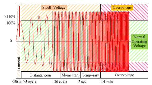
Problems of electric quality are often found in rural areas caused by lighting, switched capacitors, system maintenance, use of nonlinear devices, incorrect ground system and use of inconsistent technology in the electrical system [2-3]. These problems promote changes in electrical quality. If the devices have sensitivity towards the response this might cause failure or malfunction. Although many systems have Surge Protection Devices (SPDs) for AC surge [4-7], damage to electronic devices still occurs as seen in Fig. 1. Damages from the change of electrical quality or swell voltage occur when RMS voltage exceeds IEEE 1159 and 1100 standards [8-9] (Fig. 2). Installation of SPDs in low-voltage systems [10] cannot prevent swell voltage lower than the working level of the device, resulting in damages to smart electronic machinery. This is a big problem for electrical quality of distribution systems in PEA. Apart from the damages, swell voltage also impacts users. As a result, analysis and improvement of electrical quality must adhere to real situations of specific areas in the country.
Fig.2. Voltage Reduction Standard of IEEE Std 1159-1995
This article presents the concepts of application of a multi-stage window comparator circuit with safety mode for swell voltage control in low voltage systems through the development of a Swell Voltage Surge Suppressor (SVSS) to reduce damages to smart electronic devices conducted to distribution systems in PEA. Design of a multi-stage window comparator circuit with safety mode using high-voltage transistors [11-14] enhances the endurance of the circuit towards high voltage systems and prevents failure, resulting in improved circuit reliability.
Basic Window Comparator Circuit
Window comparator circuits (WCs) often used are IC Op-Amp, Logic gate, IC packet, IC CMOS and TTL [15-18]. The window comparator circuit type IC has low input voltage and current. It is suitable for analysing small signals. If devices inside the IC are damaged or lack qualification, the circuit will not work or work abnormally. For these IC devices, characteristics of damages inside the circuit cannot be examined. The window comparator circuit has different low-voltage levels (VLow) and high-voltage levels (Vhigh). This qualification is called Hysteresis and is used to detect the signal as the designed function. If the analogue input (Vin) is in the range of standardised electrical level, the output signal will be 1 (High). However, apart from this condition, signal output will be 0 (Low).
Window Comparator Circuit with Transistors
After the IC window comparator circuits have been applied to detect the overvoltage [19], this might damage the devices inside IC. The use of transistors in the design of window comparator circuits is important [12-14]. Today, semi-conductors have been developed for use at higher voltage. Application of high-voltage transistors with VCE ±300V of KSP42 and KSP92 transistors in the design can be adapted for other uses. Oscillator circuits made from a pair of transistors are used in window comparator design (Fig. 3). When Vin is higher than Vref_L (Vin>Vref_L), the transistor Q1 works (on) with electricity flowing through Q1, resulting in clamping voltage at R3 (VR3). The resistors, R4 and R5, are voltage divider circuits. They control the function of low voltage (Vref_L) as seen in the equation.
.
When Vin has voltage higher than Vref_H (Vin>Vref_H), the transistor Q2 will work (on) while the resistors, R1 and R2, which are voltage divider circuits, control the function of low voltage (Vref_H). When the transistor Q2 works and enters saturation, the output signal Vout =0V as seen in the equation.
.
Fig.3. Window Comparator Circuit with Transistors
Application of a window comparator circuit requires expansion of the output signal to make the output signal logic become 0 (OFF) or 1 (ON). When Vin is at the specified level, the voltage Vout at the Q3 transistor’s base is around 0.7V, resulting in electricity flowing and the clamping voltage Vce of the Q3 transistor is 0V. The Q4 transistor will not work (IC =0). Therefore, the transistor works like a switch in an open circuit or in the cut-off state, causing clamping Vce(cut-off) at the Q4 transistor equal to Vo and VP as seen in the equation.
.
When Vin is outside the standard voltage level, the voltage at the Q3 transistor’s base will be lost, causing flow of electricity (IC=0). The clamping voltage has R6 equal to ICR6, resulting in voltage at the Q4 transistor’s base while the electricity IC flows to the high position resulting in clamping voltage Vce=0V. Therefore, the transistor works like a switch in a closed circuit or in saturation state as seen in equation.
Fig.4. Window Comparator Circuit with Extended Circuit
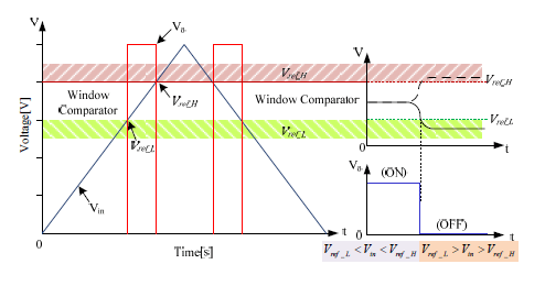
In Fig. 4, Vp is the output voltage that can control the voltage level of electronic loads. Characteristics of the output signal of a window comparator circuit with Q3 and Q4 transistors work like a switched circuit. When the signal of Vin in the windows of Vref_L and V ref_H is according to the set function as seen in Fig. 5, the output signal remains High (ON). If Vin is outside of Vref_L and V ref_H, the output signal will be Low (OFF) as seen in the equation.
.
Fig.5. Comparison of output signals of the window comparator circuit
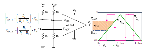
To make it simple, a block diagram similar to Op-amp was drawn with single input and output. This means 1 Opamp symbol is equal to 1-stage window comparator circuit or WCS-1 as seen in Fig. 6.
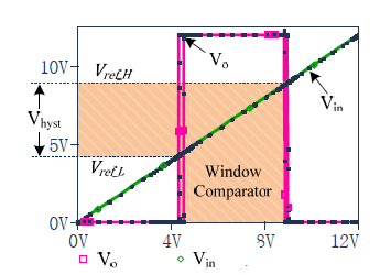
From Fig. 6, set the function of window comparator with four resistors: R1, R2, R3, and R4, connecting in the voltage divider circuit as R1 and R2 to control the function of Vref_H while R3 and R4 control the function of Vref_L. To create the signal channel of the window comparator, the difference between voltage level Vref_L and Vref_H will be called hysteresis voltage or Vhyst [18]. This could cause a change of voltage level at two positions as seen in Fig. 7. Consequently, to calculate Window Comparator Hysteresis, the voltage level should be set to eliminate the swing of the input signal Vin due to error or noise as the equation below.
.
Fig.6. Functionality of Window Comparator
Fig.7. Output Signal of Window Comparator with Hysteresis
Multi-stage Window Comparator Circuit
A multi-stage window comparator can set multi ranges of voltage level to assess the difference between Vref_L-N and Vref_H-N when an analog output signal Vin is added into the system. If it is from WCS-1 to WCS-N as the regulated function, the output signal from Vo-1 to Vo-N of any stage will be 1. Apart from this condition, the output signal will be 0 as seen in Fig. 8.
Fig.8. Multi-stage Window Comparator Circuit
Fig. 8 demonstrates the overview of the multi-stage window comparator circuit. When used to detect swell voltage, it will assist by dividing the violent level of swell voltage that enters the low voltage system. Selection of device, resistor and transistor in the circuit must be endurable. The working function must be examined and failure mode analysed to check the abnormality of physical characteristics.
Principle of Swell Voltage Control
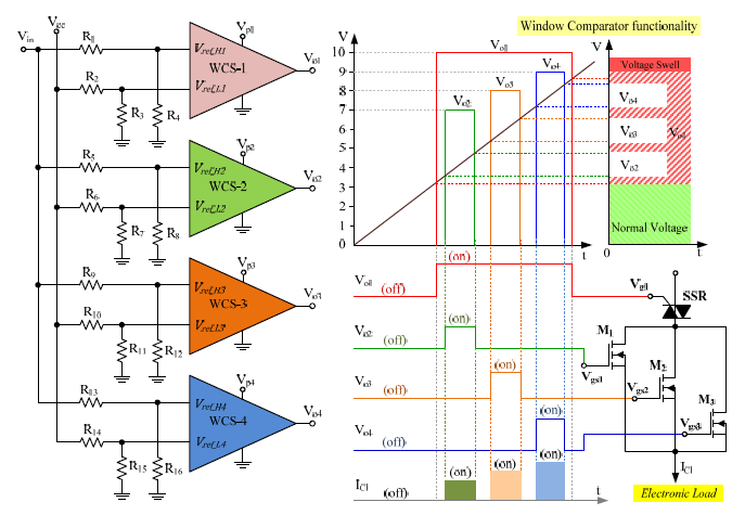
Swell voltage control by a Swell Voltage Surge Suppressor (SVSS) can be used as the electronic load that receives overvoltage in the system [20-21]. There are four sets of window comparator circuits for detecting swell voltage. Each set has a different window level. WCS-1 first detects the swell voltage. If Vin shares the same value as the window’s voltage of WCS-1, the output signal Vo1 becomes 1. When Vin rises to reach the window levels of WCS-2, WCS-3 or WCS-4, then one of the output signals at Vo2, Vo3 or Vo4 is 1. All three sets work under the window level of WCS-1 as seen in Fig. 9.
Fig.9. Multi-stage Window Comparator Circuit and Output Signal
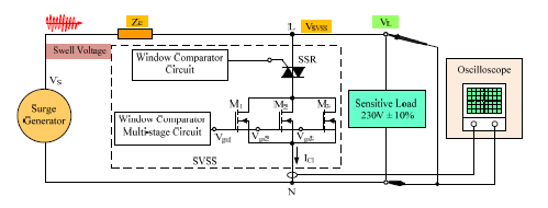
In Fig. 9, the electronic load controlled by the multi-stage window comparator circuit will work when Vin shares the same window level as WCS-1. The output signal Vo1 will force the switch of Solid-state Relay (SSR) [22] to activate (on) and when the voltage of Vin is equal to the window level of WCS-2 ,WCS-3 or WCS-4, it will cause Leakage Current (LC1) through electronic loads M1, M2 or M3, which connect in parallel. If the device at M1 level becomes damaged and the voltage Vin continues to increase, M2 and M3 still work. M1, M2, and M3 are electronic device type Power MOSFET. Here, selected SCT3080KL MOSFET with voltage between Drain– Source could reach 1,200V. It is an electronic lead that works as the energy supporter and could be compared to a load in the system. The use of MOSFET enhances the endurance of the electronic circuit to be safer, more constant and prevent dangerous failure that might occur in the system. When Vin is lower, the window comparators WCS-2 , WCS-3 or WCS-4 will cause M1, M2 or M3 to stop working, while they are working under WCS-1, until the voltage is lower than WCS-1. It also causes the SSR to stop working (off). The electricity IC1 ceases to flow. Characteristics of electronic load control of M1, M2, and M3 have different voltage control level. This affects the flow of electricity through electronic loads and helps to control the loaded voltage at the standard level in accordance with IEEE Std 1159 and IEEE Std 1100.
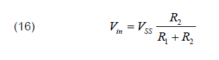
The multi-stage window comparator for swell voltage control with RMS over the standard (230V ±10%) [8-9] will be installed parallel to the power system. The swell voltage causes electricity to flow through the first rectifier circuit, which is the voltage sensor (VSS), while the resistors R1 and R2 connect to the voltage divider circuit to reduce the voltage to remain at the appropriate level. The received Vin will be added to the window comparators WCS-1 WCS-2 WCS-3, and WCS-4 respectively, as seen in equation.
.
Fig.10. Multi-stage Window Comparator Circuit for Swell Voltage Control
From Fig. 10, the voltage detector circuit by the window comparator with the safe mode will examine the voltage Vin. If Vin follows the condition, the output signals Vo1, Vo2, Vo3 or Vo4 will control electronic loads in accordance with the overvoltage level in the system. The electronic load control circuit will supply electricity and control voltage, resulting in clamping voltage at the electronic loads as seen in the equation.
.
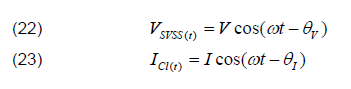
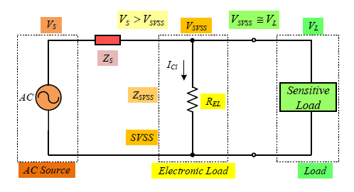
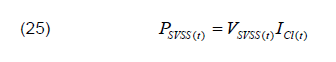
If drawing the block diagram by replacing SVSS as the resistor load (REL), when removing the sensitive load out of the circuit, it is evident that REL makes the series with the resistant (ZS) of the power distribution source by dividing from the voltage at VSVSS. As seen in Fig. 11, the electronic load pulls the power current ICl to flow through itself as a means to preserve the voltage level, VSVSS ≅ VL that is distributed to the load to remain level and not over the standard as seen in the equation.
.
The electronic load is similar to the resistor load connecting to the AC source, resulting in swell voltage and swell current as seen in the equation.
.
Fig.11. Connection of electronic loads by dividing the voltage from the power source
To calculate the clamping voltage of the electronic load circuit, see the equation.
.
For consideration of the power of electronic loads in the AC power system during the electricity flow due to swell voltage, the multiple results of voltage and short current, see the equation.
.
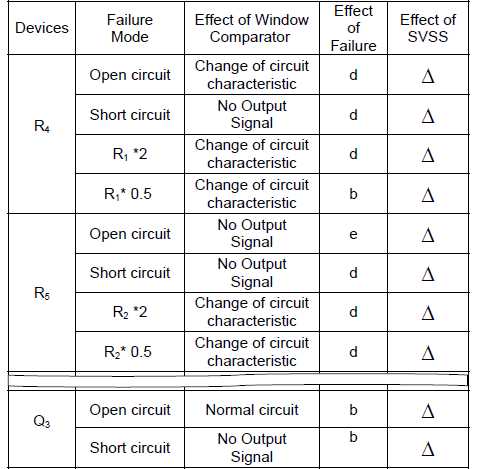
Table 1. Result of Failure Modes and Effects Analysis of the created Window Comparator Circuit
.
Notes *(0.5) and *(2) referred from the standard measurement. (a): Normal Output (b): No Output (c): window Voltage reduced (d): window Voltage increase (e): Output as Vp (f): Half reduction output Δ : no significant consequences of SVSS
Analytical Result of The Window Comparator’s Safe Mode Circuit
Failure Modes and Effects Analysis (FMEA) [23-26] is the indicator in analysis of the safe failure of the window comparator that leads to prevention of damages. The principle of the analysis has been standardised and the result confirms that the window comparator circuit will work with the safe mode. If there is any dangerous failure with any device in the window comparator or the four sets, SVSS will stop working immediately and will not cause any dangerous failure to the system. See Table 1.
Testing Result of Swell Voltage Control
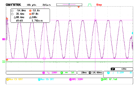
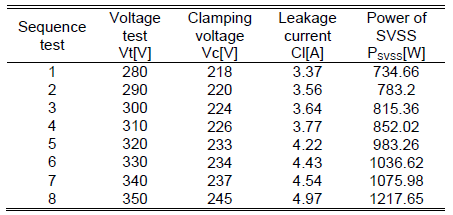
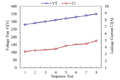
The SVSS device was tested for swell voltage control [27-29] by connecting to the top the system before distributing the voltage at 280V, 290V, 300V, 310V, 320V, 330V, 340V and 350V [20-21] and measuring the signal wave of clamping voltage at the output as seen in Fig. 12 and Fig. 13.
Fig.12. Testing the SVSS Circuit for Swell Voltage Control
Fig.13. Measurement of the model SVSS by Oscilloscope
The wave of the output signal of the multi-stage window comparator was measured for electronic load control by adding the triangle-wave signal to test its function. When the voltage reached the destined level, the output signal through the windows Vo1, Vo2, Vo3, and Vo4 to control the electronic loads in accordance with the overvoltage. See Fig. 14 and Fig. 15.
Fig.14. Output signal of multi-stage window comparator for SVSS control
The distributed AC current was at 280-350V and the frequency was 50 Hertz. The wave of the signal to test the size of overrated voltage is shown in Fig. 16. The test applied an oscilloscope to measure the signal wave of current and clamping voltage at the output before recording (Table 2).
Fig.15. Input and Output Signals of multi-stage window comparator for SVSS control
Fig.16. Testing the signal of 320V
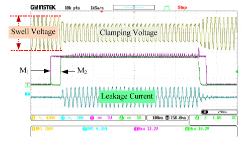
Fig.17. Input and Output signal of SVSS for Swell Voltage Control
Fig.18. Frontal expansion of swell voltage control
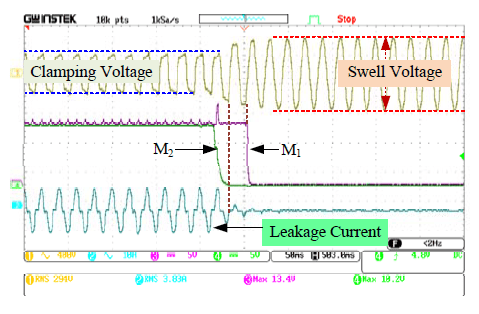
Fig. 17 shows the distributed overvoltage in the system. The signal detected CH1 as the signal wave of swell voltage and CH3 as the output signal from the window comparator with V01 as the signal forcing M1 CH4 as the output signal from the window comparator with V04 as the signal forcing M2, and CH2 as the wave of electric current ICl flowing through the electronic loads for swell voltage control. as seen in Fig. 18 and Fig. 19.
Fig.19. Rear expansion of swell voltage control
Table 2. SVSS Test Results for Swell Voltage Level Control
.
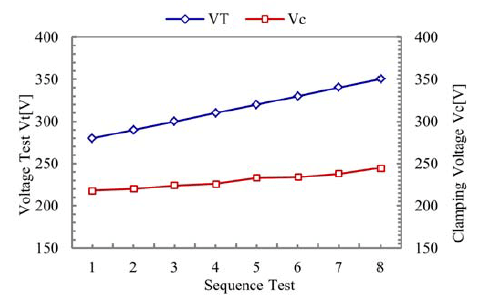
Fig.20. Graph showing the relationship between voltage test and clamping voltage
Fig.21. Graph showing the relationship between voltage test and leakage current
Fig.22. Graph showing the relationship between transient power loss and voltage test
Data were demonstrated in the graph as the relationship between voltage, electric current and electric power of SVSS for swell voltage control as seen in Fig. 20, Fig. 21 and Fig. 22 respectively.
Conclusion
This article demonstrated the multi-stage window comparator circuit as safe for swell voltage control in low voltage systems. Problems are caused by the quality and stability of the power system and might affect smart electronic devices conducted on distribution systems in PEA. The design of swell voltage level control contains the main circuit as the window comparator circuit with safe mode to detect the overvoltage level from the high-voltage transistor, with the purpose of enhancing the endurance of high-voltage. It also reduces the effect of dangerous failure in the system. The created window comparator circuit can detect voltage level and control electronic loads with safe mode. The FMEA result based on IEC 61496-1 standard, assured the working process of the device to be reliable and stable to control safety under many kinds of situations. The testing result showed that SVSS for swell voltage level control was effective by allowing the electric current to flow through itself, resulting in reduction of voltage level. The current moving through smart electronic devices was not over the standards of IEEE Std 1159 and IEEE Std 1100.
REFERENCES
[1] SB. Kjaer, JK. Pedersen, and F. Blaabjerg, “A review of single-phase grid-connected inverters for photovoltaic modules,” in IEEE Transactions on Industry Applications, 41(2005), 1292–1306 [2] D. O. Johnson, K. A. Hassan. “Issues of Power Quality in Electrical Systems,” International Journal of Energy and Power Engineering, 5 (2016), No. 4, 148-154 [3] J. Kaniewski, “Transformator hybrydowy z dwubiegunowym przekształtnikiem AC/AC bez magazynu energii DC,” Przegląd Elektrotechniczny, ISSN 0033-2097, 94 (2018), nr 5, 80-85 [4] V. Radulovic, S. Mujovic, and Z. Miljanic, “Characteristics of Overvoltage Protection with Cascade Application of Surge Protective Devices in Low-Voltage AC Power Circuits,” Advances in Electrical and Computer Engineering, 15 (2015), No. 3, 153-160 [5] IEEE Std C62.41.1-2002, IEEE Guide on the Surge Environment in Low-Voltage (1000 V and Less) AC Power Circuits, April 2003. [6] P. Hasse, Overvoltage Protection of Low Voltage Systems, 2nd ed. United Kingdom: The Institution of Electrical Engineers, 2000. [7] D. Paul, “Low-voltage power system surge overvoltage protection,” in IEEE Transactions on Industry Applications, 37 (2001), 223-229 [8] IEEE Std 1159-2009, IEEE Recommended Practice for Monitoring Electric Power Quality, November 2009. [9] IEEE Std 1100-2005, IEEE Recommended Practice for Powering and Grounding Electronic Equipment, December 2005. [10] Z. He and Y. Du, “SPD Protection Distances to Household Appliances Connected in Parallel,” in IEEE Transactions on Electromagnetic Compatibility, 56 (2014), No. 6, 1377-1385 [11] E. J. Wade, and D. S. Davidson, “Application of Transistors to Safety Circuits,” in IRE Transactions on Nuclear Science, 5 (1958), No. 2, 44-46 [12] K. Futsuhara, and M. Mukaidono, “Application of Window Comparator to Majority Operation,” in The Nineteenth International Symposium on Multiple-Valued Logic, (1989), 114-121 [13] K. Futsuhara, and M. Mukaidono, “A Realization of Fail-safe Sensor Using Electromagnetic Induction,” in Conference on Precision Electromagnetic Measurements CPEM, (1988), 99-100 [14] M. Sakai, M. Kato, K. Futsuhara, and M. Mukaidono, “Application of Fail-safe Multiple-valued Logic to Control of Power Press,” in 1992 Proceedings The Twenty-Second International Symposium on Multiple-Valued Logic, (1992), 271-350 [15] P. Sagar, P. P. R. Madhava, “A Novel, High Speed Window Comparator Circuit,” in 2013 International Conference on Circuits, Power and Computing Technologies (ICCPCT), (2013), 691-693 [16] M.W.T. Wong, and Y. Zhang, “Design and Implementation of Self-Testable Full Range Window Comparator,” in Proceedings of the 13th Asian Test Symposium (ATS2004), (2004), 1-5 [17] S. Maheshwari, “Current Conveyor Based Window Comparator Circuits,” Advances in Electrical Engineering, (2016), 1-8 [18] V. A. Pedroni, “Low-voltage high-speed Schmitt trigger and compact window comparator,” in Electronics Letters, 41 (2005), No. 22, 1213-1214 [19] Y. Zhang and M.W.T. Wong, “Self-Testable Full Range Window Comparator,” in IEEE Region 10 Conference TENCON 2004, (2004), 262-265 [20] N. Mungkung, S. Wongcharoen, C. Sukkongwari, and S. Arunrungrasmi, “Design of AC Electronics Load Surge Protection,” in International Journal of Electrical, Computer, and Systems Engineering, ISSN 1307-5179, 1 (2007), No. 2, 126-131 [21] N. Mungkung, S. Wongcharoen, K. Chomsuwan, P. Nuchuay, K. Permsupsin and T. Yuji, “Electronics Load for Voltage Swell Protection,” in Conference on Embedded Systems and Intelligent Technology, (2008), 303-307 [22] R. N. Eldine, I. Amor, A. Massoud, and L. B. Brahim, “Smart Low Voltage ac Solid State Circuit Breakers for Smart Grids,” in Global Journal of Advanced Engineering Technologies, 2 (2013), No. 3, 71-79 [23] IEC Std 60812-2018, Failure modes and effects analysis (FMEA and FMECA), 3th ed. IEC International Standard, July 2018. [24] C. Summatta, W. Khamsen, A. Pilikeaw and S. Deeon, “Design and Simulation of Relay Drive Circuit for Safe Operation Order,” in Conference on Mathematics, Engineering & Industrial Applications 2016 (ICoMEIA 2016), August 2016. [25] S. Deeon, Y. Hirao, K. Tanaka, “A Relay Drive Circuit for a Safe Operation Order and its Fail-safe Measures,” in The Journal of Reliability Engineering Association of Japan, 34 (2012), No.7, 489-500 [26] S. Deeon, Y. Hirao and K. Futsuhara, “A Fail-safe Counter and its Application to Low-speed Detection,” in The Journal of Reliability Engineering Association of Japan, 33 (2011), No.3, 135-144 [27] IEC Std 61496-1, Safety of machinery-Electro-sensitive protective equipment-Part 1: General requirements and tests, IEC International Standard, April 2012. [28] IEEE Std C62.41.1-2002, IEEE Guide on the Surge Environment in Low-Voltage (1000 V and Less) AC Power Circuits, April 2003. [29] IEC Std 6100-4-5-2014, Electromagnetic Compatibility (EMC), Part 4-5, Testing and measurement techniques, Surge immunity test, IEC International Standard, June 2014.
Authors: Mr. saktanong wongcharoen, E-mail: saktanong.w@gmail.com; Dr. Sansak Deeon, E-mail: sdeeon2013@gmail.com. Department of Electrical Engineering, Pathumwan Institute of Technology, 833 Rama1 Wangmai District, Bangkok, Thailand;
Source & Publisher Item Identifier: PRZEGLĄD ELEKTROTECHNICZNY, ISSN 0033-2097, R. 96 NR 5/2020. doi:10.15199/48.2020.05.17
Published by Konrad URBAŃSKI, Dariusz MAJCHRZAK,Poznań University of Technology
Abstract. In this paper, simulation research results of PMSM drive with open phase fault detection are presented. Proposed fault detection system is implemented using two artificial neural networks. One of them is neural model of healthy PMSM and another one generates diagnostic signals. When the fault occurs, the amplitude of current residuals increases and evaluation system returns diagnosis. In proposed system detection time is about 1 ms. Moreover, diagnosis does not depend on load state.
Streszczenie. Artykuł przedstawia wyniki badań symulacyjnych napędu PMSM z detekcją przerwy fazy. Proponowany system detekcji uszkodzeń zaimplementowano z użyciem dwóch sztucznych sieci neuronowych. Jedna z nich pełni rolę modelu neuronowego sprawnego PMSM, natomiast druga generuje sygnały diagnostyczne. W przypadku wystąpienia uszkodzenia amplituda residuów prądów wzrasta, a system ewaluacji zwraca diagnozę. Czas detekcji w przedstawionym układzie jest rzędu 1 ms. Ponadto działanie systemu nie zależy od stanu obciążenia (Detekcja uszkodzeń w napędzie z PMSM przy użyciu Sztucznej Sieci Neuronowej).
Keywords: Artificial Neural Network, PMSM, Fault detection, Electric drive. Słowa kluczowe: Sztuczna Sieć Neuronowa, PMSM, Detekcja uszkodzeń, Napęd elektryczny.
Introduction
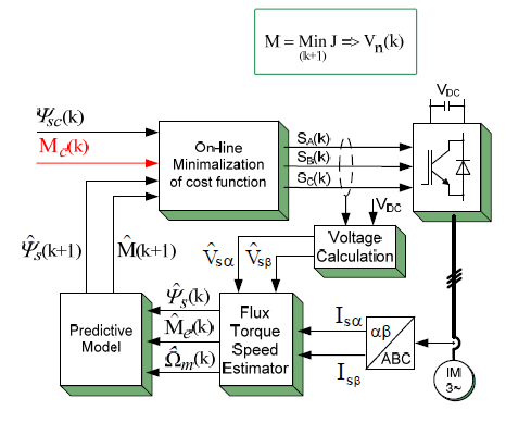
The permanent magnet synchronous motors (PMSM) are becoming increasingly popular in industry due to their high power density, low inertia and high efficiency. Thanks to their excellent dynamic performance, they are widely used in robots, machine tool, winders and similar systems that require precise speed and torque control. Nowadays, electrical drives often work in human life-critical systems, where high reliability is required [1]. In these applications the traditional control algorithms do not provide a sufficient safety, so fault tolerant control (FTC) is commonly used. FTC algorithms require information about type and location of fault [2], therefore the fault detection and diagnosis systems are necessary. There are many methods of fault detection and identification. They can be divided into signal processing based and model-based categories. First of them uses measured signals analysis methods such as spectral analysis [3] or wavelet transform [4]. In general, they only uses output signals of drive, but no input signals, so influence of input on output may be ignored [5]. Mode-based methods use information about structure and parameters of dynamic model of plant. These include state estimation methods, for example observers or Extended Kalman Filter [6]. Moreover, model parameters estimation methods like recursive last square algorithm can be used [7]. Model-based methods generate residuals, by estimating output signals (or parameters of the plant) and computing estimation error vector [8]. Next the residual evaluation system generates diagnosis. Fig. 1 presents the block diagram of model-based method of fault detection. Symbols shown in Fig. 1 are u – plant inputs, y – plant outputs, z – disturbance, f – fault, and r – generated residuals. The main disadvantage of mentioned methods is the need for a reliable model [5]. In this paper, fault detection method based on model is connected with computational intelligence methods. Presented in this paper the residual generator contains neural model of PMSM. Moreover, the residual evaluation system is also realized using the Artificial Neural Network (ANN).
Mathematical model and control structure
Dynamic model of PMSM used in this paper is given as follows:
.
Fig.1. Block diagram of model-based fault detection system
.
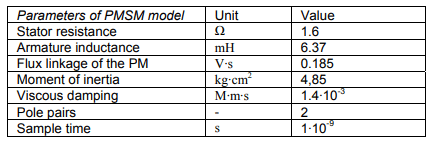
where id, iq,Ld, Lq, vd, vq – currents, inductances and voltages in d-q axes, R – winding resistance, p – pole pairs, ωr – angular speed of rotor, λ – permanent magnets flux linkage, Te– electromagnetic torque, J – moment of inertia, F – viscous friction coefficient, Tm – load torque, ϴ – rotor angular position.
Used control algorithm was Field Oriented Control (FOC) [9]. Clarke and Park transforms were used for 3 phase non-rotating frame into two coordinate rotating reference frame conversions. PI controllers were used in speed and currents control loops. Transistors gate pulses were generated using Space Vector Pulse Width Modulation (SVPWM) [9]. The block diagram of control structure is shown in Fig. 2.
Fig.2. Block diagram of Field Oriented Control with Space Vector Pulse Width Modulation
Fault detection method
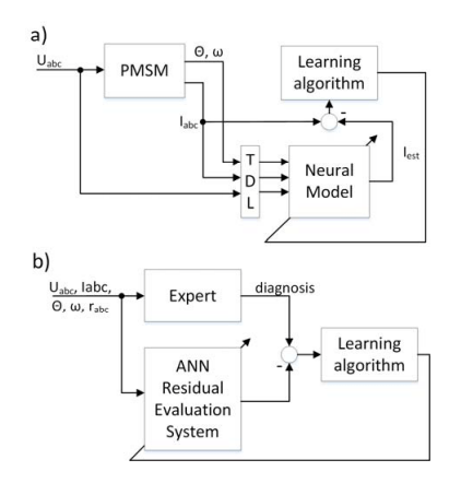
The main blocks of the system are neural model of PMSM and diagnostic module. The inputs of the both networks are phase currents, phase voltages, speed and the motor shaft position. In addition, the current residuals vector is given to the input of the diagnostic block, which returns the diagnosis. The output of the system is diagnostic signal which indicates open phase fault occurrence. The block diagram of the system is presented in Fig. 3.
Fig.3. Block diagram of neural fault detection system
In the figure, ϴ is the position, and ω is the speed. For increase of residual signal magnitude during open phase fault, in place of measured currents the weighted arithmetic mean of estimated and measured currents was applied. Used coefficients was experimentally determined and was 0.8 for estimated and 0.2 for measured values. The tapped delay line (TDL), delays voltages, speed and position samples by 0, 1 and 2 steps. It also delays currents by 1 and 2 steps. In practical applications the phase voltages are not measured. To avoid implementation of extra sensors the reference voltages can be used. In that approach system processes variables that are already used by vector control algorithm.
Signals acquired from the several simulations of healthy motor drive, working at various speeds and loads were used for training the neural model. Residual evaluation system was trained on data obtained during open phase fault simulations. A fault trigger signals were used as a target data. Neural model consists two-layer feed-forward ANN, with 6 neurons in the first layer, and 3 neurons in output layer. Activation functions are hyperbolic tangent in hidden layer, and linear in output layer. Residual evaluation system is three-layer perceptron. The first hidden layer has 14 and the second 7 neurons. Activation functions are:
linear in the first layer and hyperbolic tangent in the other ones. Both ANNs were trained with the Levenberg Marquardt algorithm [10,11] with Bayesian regularization using structures shown in Fig. 4.
Fig.4. Artificial neural network training schemes. a) neural model, b) residual evaluation system
Simulation results
The simulation studies of presented system were performed in MATLAB/Simulink environment. PM machine and power converter models were implemented using SimPowerSystems toolbox. The PMSM drive model operates using vector control, with outer loop of speed control, and inner loop of current control. The motor is fed by a voltage source inverter. It was necessary to create power converter in such a way that the open phase fault could be simulated. There was logical AND operation applied on transistors gate pulse signals, to simulate open circuit fault by holding selected ones at logical zero. The ANNs were implemented and trained using MATLAB Neural Networks Toolbox. Fundamental sample time used in simulation was 1 μs for motor and power converter models, and 100 μs for other blocks. The PWM carrier frequency was equal 10 kHz, and used “dead time” was equal 4 μs. Some sample simulation results of fault detection system behavior are shown in Fig. 5. and Fig. 6.
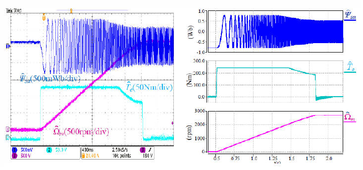
The waveforms in Fig. 5a shows phase currents during motor startup, which is working at speed 250 rad/s. In addition, at time 0.04 s, a stepwise load was attached, from zero to nominal value. At time 0.06 s open phase A fault is occurred. It is shown in Fig. 5b that fault occurrence causes residuals amplitude increase. This is because of differences between measured and estimated currents. There are some peaks in residual evaluation system output signal, as presented in Fig. 6a. It is caused by inaccurate model of electric drive. To avoid a false-positive error the 10 point moving average filter was applied. Proposed filter was defined as:
Fig.5. Simulation results of proposed neural residual generator. a) phase currents, b) residuals
Fig.6. Simulation results of proposed open phase detection system. a)Residual evaluation system output, b) filtered output, c) diagnosis
Fig.7. Impact of the time-varying load torque on false-positive error. a) phase currents, b) torque, c) residual evaluation system output, d) diagnosis
where ff – filter output signal , fraw – filter input signal, and N – number of points in average. The figure 6b presents filtered residual evaluation system output signal. Diagnosis is created by thresholding of filtered signal.
In the Fig. 7 the impact of the time-varying load torque on diagnosis is presented. After motor startup, drive is working at constant speed and load torque steps and ramps occur.
It can be seen, that peaks in residual evaluation system output signal has been filtered and diagnosis does not depend on load state. It is worth noting that fault detection system works properly from the very beginning of motor startup, so no detection disabling signals are required. Presented system can work as autonomous block in the motor drive.
Simulations at various speeds and angles has been done to examine the electrical angle of the fault occurrence impact on detection time. In table 1, there are presented the fault detection times in a case of various conditions for testing of the break in phase A.
Table 1. Detection time at different electrical angle of open phase A fault occurrence and at various speeds
.
In the most cases, detection time is less than 1 ms, except angles near 0° and 180° during phase A current zero crossing. Zero phase current caused by open phase fault cannot be distinguished from natural current zero crossing so fault detection is delayed. It is worth to add that angular velocity does not impact on detection time.
Conclusions
In this paper, an open phase fault detection system has been introduced. Presented method was verified by simulation research and gave good results. Proposed detection system is fast – detection time is about 1 ms. Short time of fault detection allows to enable FTC algorithm before eventual drive damage, which may occur due to high torque pulsation during open phase state. Presented system processes variables which are already used by vector control algorithm, avoiding the use of extra sensors. Moreover, transient states of drive system and motor speed do not influence diagnosis.
Appendix. Parameters of used Permanent Magnet Machine model
.
REFERENCES
[1] Ertugrul N., Soong W., Dostal G., Saxon D., Faulttolerant motor drive system with redundancy for critical applications, proceedings of the IEEE Power Electronics Specialists Conference 2002 (PESC ‘02), pp. 1457-1462, 2002. [2] Łuczak D., Siembab K., Comparison of fault tolerant control algorithm using space vector modulation of PMSM drive, proceedings of the 16th Mechatronika, pp. 24-31, 2014. [3] Khlaief A., Boussak M., Gossa M., Phase faults detection in PMSM drives based on current signature analysis, XIX International Conference on Electrical Machines (ICEM), pp. 1-8, 2010. [4] Riba J.R., Rosero J.A., Garcia A., Romeral L., Detection of demagnetization faults in permanent-magnet synchronous motors under nonstationary conditions, IEEE Transactions on Magnetics, vol 45, no. 7, pp. 2961-2969, 2009. [5] Liu X.Q., Zhang H.Y., Liu J., Yang J., Fault Detection and Diagnosis of Permanent Magnet DC Motor Based on Parameter Estimation and Neural Network, IEEE Transactions on Industrial Electronics, vol 47, no. 5, pp.1021-1030, 2000. [6] Park B.G., Jang J.S., Kim T.S., Hyun D.S., EKF based fault diagnosis for open-phase faults of PMSM driver, proceedings of the IEEE In Power Electronics and Motion Control Conference, pp. 418-422, 2009. [7] Park B.G., Kim R.Y., Hyun D.S., Fault diagnosis using recursive least square algorithm for permanent magnet synchronous motor drives, in Power Electronics and ECCE Asia (ICPE & ECCE), pp. 2506-2510, 2011. [8] Korbicz J., Koscielny J.M., Kowalczuk Z., Cholewa W., Fault Diagnosis. Models, Artificial Intelligence, Applications, Springer ,Berlin 2004. [9] Quang N.P., Dittrich J.-A., Vector Control of ThreePhase AC Machines, Springer, Berlin 2008. [10] Levenberg K., A Method for the Solution of Certain Non-Linear Problems in Least Squares. Quarterly of Applied Mathematics 2, pp. 164–168, 1944. [11] Marquardt D., An Algorithm for Least-Squares Estimation of Nonlinear Parameters. SIAM Journal on Applied Mathematics 11 (2), pp. 431–441, 1963.
Authors: dr inż. Konrad Urbański, Politechnika Poznańska, Instytut Automatyki i Inżynierii Informatycznej, ul. Piotrowo 3a, 60-965 Poznań, E-mail: Konrad.Urbanski@put.poznan.pl; mgr inż. Dariusz Majchrzak, Automatyki i Inżynierii Informatycznej, ul. Piotrowo 3a, 60-965 Poznań, E-mail: Dariusz.zb.Majchrzak@doctorate.put.poznan.pl.
Source & Publisher Item Identifier: PRZEGLĄD ELEKTROTECHNICZNY, ISSN 0033-2097, R. 93 NR 6/2017. doi:10.15199/48.2017.06.06
Published by HSB, Power quality — basics Commercial property, One State Street P.O. Box 5024 Hartford, CT 06102-5024 Tel: (800) 472-1866. Website: HSB.com
Introduction
Power quality is a general term used to describe the compatibility between connected equipment and its electrical supply. The supply system can be affected by changes to the frequency or amplitude of the voltage, the balance between phases on a three-phase system, and distortion levels of the original signals. The characteristics that are important and what can be tolerated by the connected equipment can vary from facility to facility.
Most electro-mechanical equipment is robust and can handle minor power quality related issues with little or no effect on operations. Electronic equipment is very susceptible to power quality related issues. Due to the shift in the type of loads from electro-mechanical to electronic, power quality is a real concern in all types of applications. This includes hospitals, universities, commercial buildings, and industrial facilities.
Poor power quality
An ideal power source offers a continuous, smooth sinusoidal voltage. Typical power quality issues include:
• Voltage transients (surges) • Harmonics • Voltage sags • Voltage swells • Voltage interruptions
Typical power quality issues. Image by HSB
The effects of poor power quality are based on the length, magnitude, and timing of the issue as well as the sensitivity of the connected equipment. Poor power quality can result in process interruptions, data corruption, data loss, malfunctioning of computer controlled equipment, and overheating of electrical equipment.
Causes of poor power quality
You might think that poor power quality is primarily the result of weather and utility-related disturbances. However, studies have shown that issues such as lightning, other natural phenomena, and utility operations, account for only a small portion of all electrical disturbances.
A large portion of electrical disturbances are from internal sources or from neighboring businesses that share the same building or are in close proximity. Internal sources can be fax machines, copiers, air conditioners, elevators, and variable frequency drives.
The conditions below are considered warning signs for potential power quality issues in a building. These conditions do not guarantee a problem; however, a building with these conditions will have an increased likelihood of having power quality issues.
• History of power-related issues • Poorly maintained electrical system • Failure of surge protection equipment • Weather and utility disturbances are common • High concentration of electronic equipment • Infrared surveys which identify excessive current flow (heat) on grounding conductors and/or system neutrals • Repeated and random equipment malfunctions, failures, tripped breakers, or blown fuses with no identified causes • Overheated equipment • Frequent switching to backup power systems • Lost data or data corruption • Premature equipment failures
Solutions
Each type of business will have a different sensitivity level to poor power quality and will have different sources of poor power quality. However, common to all businesses is the importance of a well-maintained electrical distribution and grounding system. The importance of these systems cannot be overstated. When addressing potential or actual power quality issues, the power and grounding system should be the first item addressed. This will improve personnel safety, allow for the proper operation of surge protection devices, minimize the potential for currents on neutral conductors, and provide a common reference plane for electronic equipment.
Once the power and grounding system deficiencies have been addressed, the next steps include power quality inspections, surveys, and the selection and installation of appropriate mitigation equipment.
Inspections are a means to understand a facility from a power quality standpoint. This understanding can be gained by noting:
• Type of equipment installed • Concentration of computer and electronic equipment • Presence of welders, power factor correction capacitors, or variable frequency drives • Heat discoloration of electrical equipment • Communication and control wiring in close proximity to power wiring • Condition of the grounding system • Presence of surge protection installed on power and data lines
Surveys typically involve monitoring and recording the electrical system of a building or a specific area of a building. Reviewing and analyzing the data from the survey helps to determine if a problem exists. The types and severity of problems will dictate the appropriate power quality mitigation strategy.
Power quality inspections and surveys should only be completed by competent power quality professionals.
In many commercial or light industrial businesses, only a few loads are affected by power quality issues. By identifying the most vulnerable loads during a survey, targeted mitigation techniques can be applied.
A wide variety of power quality correction products is available utilizing a range of technologies to correct power quality issues. Common mitigation techniques include surge protection devices, isolation transformers, voltage regulators, motor-generators, standby power supplies, uninterruptible power supplies, and harmonic filters. Each technique has advantages and disadvantages, and should be applied based on its ability to solve a problem identified in the power quality survey and analysis.
Author: HSB, a Munich Re company, is a technology-driven company built on a foundation of specialty insurance, engineering, and technology, all working together to drive innovation in a modern world.
Published by Aleksander JAKUBOWSKI1, Natalia KARKOSIŃSKA–BRZOZOWSKA2, Krzysztof KARWOWSKI1, Andrzej WILK1, Gdańsk University of Technology, Faculty of Electrical and Control Engineering (1), Civil and Environmental Engineering (2)
Abstract. The paper presents possible environmental, energy and economical gains implied by replacing conventional traction vehicles with independently powered electric multiple units (IPEMU) on partially electrified suburban railways. IPEMUs can operate in two modes of power supply – using an overhead catenary or the on–board battery storage. Appropriate computer simulations were carried out in the Matlab program, indicating the parameters of storage electric multiple units.
Streszczenie. W artykule wskazano na potencjalne korzyści energetyczne, środowiskowe i częściowo ekonomiczne wynikające z zastąpienia konwencjonalnych jednostek trakcyjnych nowymi zasobnikowymi zespołami elektrycznymi mogącymi się poruszać na liniach kolejowych częściowo niezelektryfikowanych. Zespoły te mogą pracować w dwóch trybach – zasilania sieciowego lub zasobnikowego. Przeprowadzono odpowiednie symulacje komputerowe w programie Matlab wskazując na parametry zasobnikowych zespołów trakcyjnych. Zasobnikowe zespoły trakcyjne w transporcie podmiejskim
Keywords: railway electric traction, vehicle hybrid power, energy storage devices, computer simulation. Słowa kluczowe: elektryczne pojazdy szynowe, hybrydowe zasilanie pojazdu, zasobniki energii, symulacja komputerowa.
Introduction
Improved versions of electric rail vehicles have been implemented for over 100 years, capable of crossing routes on non–electrified railway sections. The AT 3 series of two– car electric battery traction unit, known as Wittfeld after the name of the designer, eng. Gustav Wittfeld [1] is an interesting vehicle from the beginning of the 20th century. The train, which could seat 90 passengers, was powered by two 62 kW motors and reached speeds of up to 60 km/h with a tare weight of 60 t. In Gdańsk Pomerania region, AT 3 units most often serviced suburban traffic. Subsequent modernizations extended the range of the units up to 300 km. In the 1950s, worn–out battery rail–cars were withdrawn from line use in Poland.
Current global trends point to potential energy, environmental and partly economic benefits resulting from the replacement of conventional DMU (Diesel Multiple Unit) traction units with new BEMU (Battery Electric Multiple Unit) electric vehicles, and especially IPEMU (Independently Powered Electric Multiple Unit) that can run on partially non–electrified lines [2–8]. DMU and BEMU vehicles are operated on non–electrified lines. IPEMU vehicles can work in two modes – overhead contact line or storage supply. On electrified sections, these assemblies draw energy from the overhead contact line for vehicle propulsion, non–traction needs and energy storage charging, while on non– electrified sections they consume energy from the accumulator, which is recharged during regenerative braking. As energy storage, Li–ion batteries are used most often, and sometimes as a hybrid storage in combination with supercapacitors [9, 10]. Vehicle power systems based on fuel cells and hybrid storages are also considered in the literature [2].
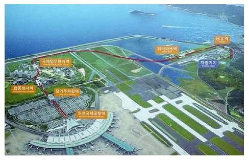
An example of the Tri–City (Gdańsk–Sopot–Gdynia) agglomeration railway line was selected for the sake of analysis and simulations presented below. A short 8– kilometer section of the single–track passenger line on the Gdynia Chylonia – Gdynia Port Oksywie route was considered, on which revitalization is planned that could reduce heavy traffic at rush hours (Fig. 1). On–board battery storage of IPEMU units charged from the catenary line while traveling on the Gdynia Główna – Gdynia Chylonia section of the Urban Rapid Railway (pol. Szybka Kolej Miejska, SKM) line would allow for further travel to the Port Oksywie station and return travel without the need to build electrical traction infrastructure [11].
Fig.1. The route of the non–electrified Gdynia Chylonia – Port Oksywie railway line
In the Tri–City agglomeration you can find many sections of the line with similar features as, for example, regional line No. 213 Reda – Hel with a length of 62 km with great touristic importance. The IPEMU unit can be supplied from the catenary line on the Gdynia Główna – Reda section, which is enough to travel from Reda to Hel station. To charge the vehicle before the return trip, a charging station was assumed to be built to charge the unit while stationary. Similar railways can also be found in other national agglomerations.
Electrical drivetrain structure
Virtually all electric multiple units (EMUs) built nowadays use an overhead contact line or a third rail for power supply. Vehicles operating in urban rail networks in Poland utilize DC line voltage of 3000 V. Thus, the construction and maintenance of a costly railway electrification system is necessary. However, depending on localization, unobstructed construction works may be impossible. The impact of electric catenary on the environment needs also to be taken into account.
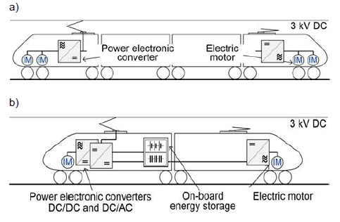
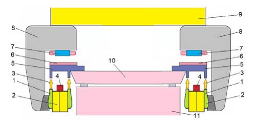
Electric multiple units are characterized by drivetrain spread over all carriages, with numerous induction motors, installed in pairs in motorized bogies and fed by inverters (Fig. 2a). Such design allows for wide–range tractive effort regulation with good dynamics and regenerative braking.
Therefore, equipping EMU with on–board energy storage (Fig. 2b) that allows to travel through non– electrified route sections might be worthwhile. Such solutions were implemented in trolleybuses and are widely used [12].
Fig.2. Examples of EMU drivetrain layout: a) conventional; b) light rail vehicle with on–board storage
Fundamental drawbacks for using energy storages in railway vehicles are the large size and weight of such devices, and the necessity of additional energy converter usage. In comparison to a vehicle supplied by an overhead line, IPEMU could have limited passenger space and slightly worse energy efficiency. Therefore, onboard storage applications are limited to light rail vehicles with various drivetrain design.
Vehicle model
Energy consumption analysis of rail vehicle equipped with on–board battery storage has been conducted on the basis of train run calculations [13–15]. For this task, a simulation program was developed using Matlab/Simulink software. Thanks to modular structure of the program, editing input parameters can be easily done, allowing for multiple cases analysis (Fig. 3).
Fig.3. Simplified block diagram of IPEMU run simulation program
Calculations are based on vehicle movement dynamics model, described by equation
.
where: a – acceleration, v – velocity, s – distance, z – control function, F – tractive effort, W – motion resistance, m – vehicle mass, k – rotational mass coefficient.
which is calculated by integrating acceleration a(t). Tractive effort F is set by control function z(s, v, t), with output limited to the range determined by rated torque and speed of the electric drivetrain. Motion resistance W(v,s) consists of fundamental Wz(v) and additional Wd(s) components – the former represents air drag, friction forces and rolling resistances (dependent on velocity), the latter reflects resistance forces from railroad track geometry curvature and inclination.
It was assumed, that acceleration and braking are realized with full available tractive effort; to simplify calculations, electric–only braking was considered. The velocity profile was set by control function z(s, v, t) which determines the relation between cruising and coasting phase, acceleration/braking dynamics as well as station stationary time. The control function program has been designed with compatibility with various drivetrain models and optimizing algorithms in mind.
Electrical energy usage is calculated by integrating electrical power, which is equal to mechanical power (computed by multiplication of traction effort and movement velocity) divided by drivetrain efficiency factor
.
where: Ez– energy consumed, η – drivetrain efficiency factor, pn – power of auxiliary loads, T – analyzed run time.
In order to estimate more accurately the energy consumption, a changing efficiency value of η(F, v) was adopted, using a predetermined table expressing the dependence of the propulsion efficiency on the torque produced by the engines and their angular velocity. The value of the power of the vehicle’s own needs has been defined at a constant level.
Energy recuperated during electric braking of the analyzed vehicle is computed as
.
Onboard battery storage has been represented by a battery model, defined in Simscape/SimPowerSystems library. Its capacity was calculated in order to allow the vehicle to cover the analyzed route in both directions, without using an overhead line nor charging the battery underway. A fully charged state of batteries at the beginning of non–electrified route was assumed.
Energy requirement for IPEMU on the analyzed railway line
Initial run calculations were conducted for 2 MW, 4– section electric multiple unit (Fig. 2a), which is a standard formation for trains in urban rail operating in Poland.
Hypothetically, such conventional vehicle could have on–board battery storage installed, so it can operate on local non–electrified line between stations Gdynia Chylonia and Gdynia Port Oksywie (15,7 km round trip, station numbers – Fig. 1). The route is characterized by relatively small differences in elevation and the speed limit is set at 70 km/h for most of its length. Entire drivetrain parameters utilization was assumed, so acceleration and braking were realized with maximum available tractive effort, also distance between stations was covered with maximum speed allowed (without coasting). The computed speed waveform is shown in Fig. 4a.
Maintaining desired velocity profile requires adequate power supply, which needs to be provided by on–board battery storage. Thus, values of battery capacity and maximum continuous discharge current are the critical factors in storage design (Fig. 4b).
On–board battery storage with parameters allowing conventional EMU for operation under assumed conditions would mass about 18 t. The volume of the storage is also significant – almost 20 m3. Equipping a vehicle with such a massive device would be impractical.
Fig.4. Conventional EMU run waveforms (Fig. 1): a) train velocity and intermediate stops; b) electrical power and energy usage
For further analysis, based on 2– section DMU similar to Pesa SA132–class (produced by PESA Bydgoszcz SA), a light rail vehicle was considered. The hypothetical vehicle would be powered by two 350 kW induction motors, sufficient for maximum speed of 100 km/h. Assuming that electric motors with inverters would replace diesel engines with torque converters and fuel tanks, 80 t net weight of vehicle was increased by 10 t (estimated weight of Li–ion battery storage).
Calculations were performed for two velocity profiles – trapezoidal, without coasting (Fig. 5) and energy–efficient (coasting until braking zone or speed dropping below 60 km/h, Fig. 6).
Results of the storage operation simulation are shown in Fig. 7. At the end of the analyzed run, the state of charge dropped to 78% – batteries were under no risk of deep discharge despite the fact that the storage was not recharged underway. Therefore, the assumed battery storage parameters are sufficient for a vehicle to cover the analyzed route without motion dynamics limitations. Also, there is no need for charging station construction. It is worth noting, that the size of battery storage could be reduced while prolonging its lifespan by equipping supercapacitors, which would absorb regenerative braking energy and provide additional power during acceleration.
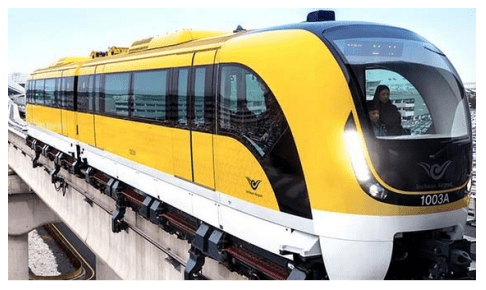
Application study and investment costs
In existing Japanese [19] and British IPEMU applications, two–segment lightweight vehicles with a mass of approx. 40 t, number of passengers 130, maximum speed of 100 km/h and acceleration of 1.2 m/s2 were adopted on agglomeration lines. An interesting European vehicle offer is the Bombardier Talent 3 intended for German and Austrian railways with much higher parameters – necessary rather for regional transport (3 units, 140 km/h, 170 seats) [20].
Fig.5. IPEMU parameters on the selected railway line without coasting: a) waveform of velocity; b) waveforms of energy and power
Fig.6. IPEMU parameters on the selected railway line with energy– efficient ride: a) waveform of velocity; b) waveforms of energy and power
Fig.7. Waveforms of currents, voltage and state of charge on– board storage: a) when passing the train without coasting; b) at the energy–saving passage
According to the manufacturer, Talent 3 generates noise and vibrations level 7 dB lower than DMU vehicles, does not emit NOx and indirectly generates CO2 only in power plants. The installed energy storage increases the vehicle’s energy efficiency compared to classic EMUs as a result of braking energy recovery and starting support. To compare the costs of purchasing Talent 3, the prices of domestic producers’ delivery were analyzed as part of tenders from 2016 for EMU and DMU vehicles for the Wielkopolskie, Śląskie, Mazowieckie and Przewozy Regionalne railway companies as well as for Poznań Metropolitan Railway. The average purchase costs are summarized in Table 1. In lines 2 and 3, there are approximate values which, together with the lack of electrification cost of the sample line (line 4) indicate the advantages of IPEMU. The full analysis of the legitimacy of choosing the type of traction unit should include the cost of the entire Life Cycle Cost, which for IPEMU is still difficult to determine.
Summary
The simulation analyses carried out indicate that on both urban and suburban lines it may be beneficial to introduce electric storage traction units of the IPEMU type to service passengers. Estimated costs presented in Tab. 1 indicate the profitability of purchasing one IPEMU instead of classic DMU while discarding 8 km section electrification. The purchase of a classic electric multiple unit together with the electrification of the section in question is similar in price to IPEMU without catenary line. However, the purchase of a larger number of IPEMUs can be economically justified if they are also used to support other non–electrified sections, e.g. Gdańsk Wrzeszcz – Airport, Rumia – Hel and similar. This relation of investment costs can be a challenge for domestic rail vehicle manufacturers in the construction of light IPEMU with technical parameters sufficient to operate on both urban and suburban lines.
Table.1 Average costs of purchase, transport and CO2 emissions of trainsets in Polish national conditions DMU
.
REFERENCES
[1] Jerczyński M., Nasz portret: wagon akumulatorowy typu„Wittfeld”, Świat Kolei 03 (1995) [2] Pagenkopf J., Kaimer S.: Potentials of alternative propulsion systems for railway vehicles – a techno–economic evaluation, Ninth International Conference EVER, 2014 [3] Ghaviha N., Bohlin M., Holmberg C., Dahlquist E., Speed profile optimization of catenary–free electric trains with lithium–ion batteries, Journal of Modern Transportation, 2019 [4] Furuta R., Kawasaki J., Kondo K., Hybrid traction technologies with energy storage devices for nonelectrified railway lines, IEEJ Transactions on Electrical and Electronic Engineering, Vol. 5, Issue 3, 2010, 291–297 [5] H. al–Ezee, C. Gould, S. B. Tennakoon, Novel method for energy management for catenary free system operation, 53rd International Universities Power Engineering Conference, 2018 [6] Y. Kono, N. Shiraki, H. Yokoyama, R. Furuta, Catenary and storage battery hybrid system for electric railcar series EV–E301, International Power Electronics Conference, IPEC, 2014 [7] Shao–bo Yin, Li–jun Diao, Wei–jie Li, Rong–jia He, Hai–chen Lv, On board energy storage and control for inter–city hybrid EMU. 43rd Annual Conference, IECON 2017 [8] F. Becker, A. Dämmig, Catenary free operation of light rail vehicles – topology and operational concept. 18th European Conference EPE’16 ECCE Europe, 2016 [9] Long Cheng, Wei Wang, Shaoyuan Wei, Hongtao Lin, Zhidong Jia, An improved energy management strategy for hybrid energy storage system in light rail vehicles, Energies 2018 [10] Radu P. V., Szelag A., Steczek M., On–Board energy storage devices with supercapacitors for metro trains – case study analysis of application effectiveness. Energies, 2019, 12, 1291 [11] Telecki M., Studium zastosowania zasobnikowych elektrycznych jednostek trakcyjnych na tworzonej pasażerskiej linii kolejowej do północnych dzielnic Gdyni. Praca dyplomowa. Politechnika Gdańska, 2018 [12] Bartłomiejczyk M., Dynamic charging of electric buses. De Gruyter, 2019 [13] Karwowski K. (red.), Energetyka transportu zelektryfikowanego. Poradnik inżyniera. Wyd. Politechniki Gdańskiej, Gdańsk 2018 [14] Bartłomiejczyk M., Mirchevski S., Jarzębowicz L., Karwowski K., How to choose drive’s rated power in electrified urban transport? 17th European Conference, EPE’17 ECCE Europe, 2017 [15] Jakubowski A., Jarzębowicz L., Karwowski K., Wilk A., Efektywność energetyczna pojazdu szynowego w różnych warunkach obciążenia, TTS Technika Transportu Szynowego, 12 (2018), 44–48 [19] Takiguchi H., Overview of series EV–E301 catenary and battery–powered hybrid railcar, JR EAST Technical Review No. 31 (2015) 27–31 [20] Laperrière P., Realize your vision with Bombardier TALENT 3 BEMU, APTA Rail Conference, 2019
Authors: mgr inż. Aleksander Jakubowski, Politechnika Gdańska, Wydział Elektrotechniki i Automatyki E-mail: aleksander.jakubowski@pg.edu.pl; mgr inż. Natalia Karkosińska– Brzozowska, Politechnika Gdańska, Wydział Inżynierii Lądowej i Środowiska, E-mail: natalia.brzozowska@pg.edu.pl; dr hab. inż. Krzysztof Karwowski, E-mail: krzysztof.karwowski@pg.edu.pl; dr hab. inż. Andrzej Wilk, E-mail: andrzej.wilk@pg.edu.pl; Politechnika Gdańska, Wydział Elektrotechniki i Automatyki, ul. Narutowicza 11/12, 80–233 Gdańsk
Source & Publisher Item Identifier: PRZEGLĄD ELEKTROTECHNICZNY, ISSN 0033-2097, R. 96 NR 4/2020. doi:10.15199/48.2020.04.33
Published by Piotr WOŹNIAK, Politechnika Łódzka, Instytut Systemów Inżynierii Elektrycznej
Abstract. This article presents simulation tests showing the benefits of using an additional energy storage device in the form of a supercapacitor in a hybrid car. An original power flow control system was proposed. The main emphasis was placed on determining the driving characteristics, emissions of harmful substances, fuel consumption and increasing the service life of batteries by limiting rapid changes in the charging and discharging currents and the operating temperature of the cells.
Streszczenie. W artykule przeprowadzono badania symulacyjne pokazujące korzyści płynące z zastosowania dodatkowego zasobnika energii w postaci pakietu superkondensatorów w samochodzie z napędem hybrydowym. W tym celu zaproponowano oryginalny system zarządzania energią. Główny nacisk położono na określenie właściwości jezdnych, emisji szkodliwych substancji, zużycia paliwa oraz wydłużenie okresu użytkowania akumulatorów poprzez ograniczenie gwałtownych zmian prądów ładowania i rozładowania oraz temperatury pracy ogniw. (Wykorzystanie hybrydowych zasobników energii w pojazdach z napędem hybrydowym: projekt strategii zarządzania energią oraz badania porównawcze)
Keywords: hybrid vehicles, supercapacitors, energy management systems. Słowa kluczowe: pojazdy hybrydowe, superkondensatory, systemy zarządzania energią.
Introduction
Increased fuel prices and high stringent requirements for harmful emissions in recent years have made electric and hybrid vehicles more popular. In the first quarter of 2019, a further increase in interest in cars with alternative power supply was visible in Europe. Sales of electric vehicles (EV) increased by 87.5% compared to the first quarter of 2018, and hybrid vehicles (HEV) by 33%. HEV vehicles accounted for around 4.7% of market share, while EV vehicles around 2%. One way to reduce emissions of harmful substances and to comply with applicable standards “downsizing”, i.e. reducing the capacity of internal combustion engines and the use of a turbine or compressor boost. However, this is not advantageous, because the motor often works in conditions of high overload and adversely affects its durability. A much better solution is to support traditional internal combustion engines with an electric drive, i.e. using a hybrid drive (HEV) or elimination of the internal combustion engine and the use of electric drive (EV). Hybrid cars combine the best features of vehicles with an internal combustion engine and cars with electric drive such as: long range, high power, lower fuel consumption, lower emissions [1]. Batteries used in electric and hybrid vehicles lose their performance over time. This is due to redox reactions occurring, overcharge, changes in internal and external environment parameters. They work well when they are charged/unloaded monotone [2, 3]. If the vehicle suddenly accelerates or brakes, the battery cannot be discharged/charged quickly enough. High battery current, especially when acceleration / deceleration is repetitive (when driving in the city) can have a detrimental effect on electrolyte and shorten battery life [2]. The price of batteries is a large part of the value of the entire car and their replacement is associated with high costs. A large number of charging cycles and use in improper conditions cause their degradation and reduction of capacity. Therefore, it is important to properly control the charging process of the battery pack [4].
Unlike batteries, supercapacitors (ultracapacitors) have a low energy density, which means that they cannot be used as the primary power source. Lithium-ion batteries can store about 20 times higher energy density than supercapacitors. Supercapacitors are also not suitable for long-term energy storage due to the fact that the self-discharge speed of supercapacitors is much higher than for lithium-ion batteries (up to 10-20 percent of charge per day). Although they cannot store as much energy and for as long as lithium-ion batteries of comparable size, their advantage is the ability to charge and discharge in a short time, in some cases the charging time is up to 1000 times shorter than the time of charging a battery with similar capacity.
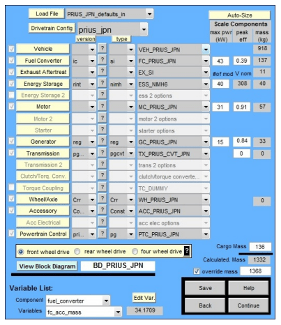
Fig.1. Advisor menu for the original Toyota Prius model
Supercapacitors therefore have a much higher power density than batteries. That is why they are well suited for applications that require frequent charging and discharging cycles, as well as operation at extreme temperatures. In China, some hybrid buses use supercapacitors to increase acceleration, and in the case of trams, these energy reservoirs allow travel from one stop to another, the charging process takes place at the stops. A hypothetical electric car will be considered to justify the use of supercapacitors. It can move with an average power of about 20 kW, however, during rapid acceleration it requires a peak power several times higher, e.g. 100 kW. Although this power level is only needed for a short time, it means that the vehicle needs additional batteries [5, 6, 7]. Supercapacitors can provide this power required for acceleration, while the battery will provide average power during normal driving, which means that generally the vehicle requires a smaller battery. In the world literature, hybrid power systems using batteries and supercapacitors are mainly used in cars with a serial or parallel hybrid drive and cars with only electric drive (EV) [1, 2], including public utility vehicles.
Technologies used
All tests were carried out using the ADVISOR simulation program, developed at the National Renewable Energy Laboratory (NREL – USA) and operating in the MATLAB environment [8]. This software is widely used for research purposes in many academic centers, e.g. [9, 10, 11, 12, 13].
In the main program menu (Fig. 1) it is possible to freely configure the vehicle, for which simulations will be carried out.
As part of the work described in the article, the first-generation Toyota Prius hybrid car model embedded in the ADVISOR program was tested, which entered serial production in 1997. This model and its parameters were adopted as a reference for research consisting in modification of the power supply system aimed at optimizing the use of energy storage in terms of fuel consumption and emissions of harmful substances such as hydrocarbons (HC), carbon oxides (CO), nitrogen oxides (NOx) and solid particles (PM). And also extending the battery life by lowering their operating temperature, charging / discharging cycles and other parameters affecting driving comfort, such as hill climbing ability.
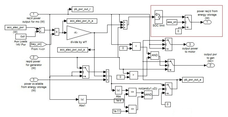
Fig.2. Toyota Prius block diagram before modificationFig.3. Toyota Prius power bus before modification
Vehicle parameters and modifications
Standard first generation Prius is powered by Ni-MH rechargeable batteries (1.2V cells, 6 cells connected together in a module, 40 modules). The vehicle modification consists in adding an additional energy storage in the form of a supercapacitors package (Maxwell PC2500 – 2700 F 2.5V). The vehicle model includes the mass of the supercapacitors module. The block diagram of the car built in ADVISOR before modification is shown in Fig. 2. Figure 3 shows the power bus model (block ‘prius power bus ‘ in Fig. 2). The block diagram (Fig. 2) and the power bus (Fig. 3) have been modified to add the energy storage. To add a second energy store, the block name and all parameters and variables starting with the prefix ‘ess_’ to ‘ess2_’ have been changed. This was necessary to avoid conflicts with the battery pack model. In the developed strategy for controlling energy storage, the input parameters are: the absolute value of the power for which there is demand at a given moment from energy storage devices (or which is available for energy storage), its sign (a positive value means discharge, and a negative charge, according to the convention adopted in the environment used), restrictions imposed on SOC (state of charge) for both storage tanks and the rate of power change over time (derivative). In addition, the information on which energy storage was previously used is included and restrictions on switching on the battery container are imposed when large instantaneous values of the charging or discharging current are required. This last action is to extend the life of the energy storage, because limiting the on/off cycles also leads to a lower average operating temperature. The possibility of each energy storage unit operation has been taken into account, and with increased power demand at a given moment, as well as in the case of a large amount of recovered power available, simultaneous operation of both tanks is possible, but the preference is always to use the current capabilities of supercapacitors .
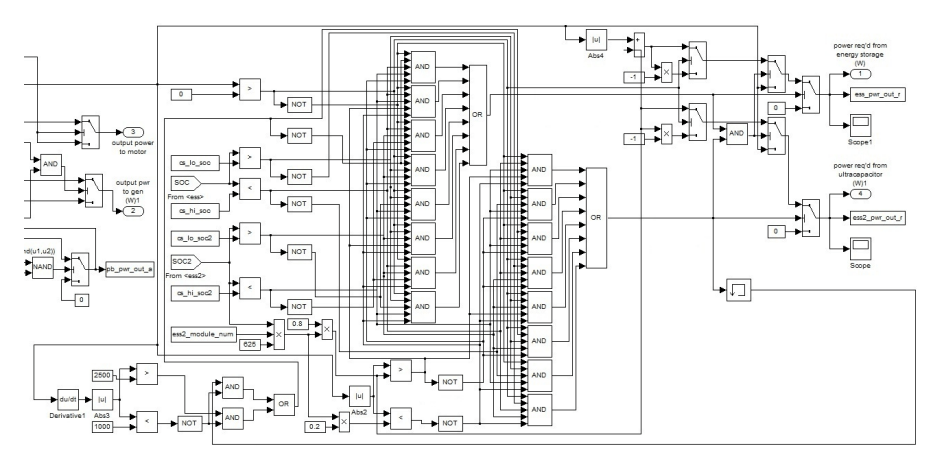
To prevent frequent switching between energy storage, two hysteresis loops were used in the control strategy. In the first loop, the current power derivative value and its belonging to the ranges defined by the two values are checked (e.g. 1000, 2500 – these values may be variable, what is more, in practice they can be determined by the driver based on the knowledge of the route, its profile and traffic) and on this basis the preference for energy storage is determined. In the second hysteresis loop, the preference of energy storage is determined depending on the absolute power value in relation to the estimated supercapacitor power. Designed control system (number of inputs 8, outputs 2), including logic after maximum reduction of Boolean expressions has been implemented in Simulink and includes: 31 logic gates (AND, OR, NOT), 10 comparison systems, 6 multipliers, derivative determination block, 2 blocks for absolute value determination and summation system. As a result of its operation, a binary signal is obtained defining the state (on/off) of each energy storage in the next time step. This allows the available/required power to be distributed to energy storage. The fragment marked with a red frame in Fig. 3 has been changed in the power bus. Figure 4 shows the modified part of the power bus. If there is a high demand for power, e.g. rapid acceleration, we use an additional energy storage in the form of a supercapacitor. During calm driving, energy is taken from the main power source.
Fig.4. Modified part of the power bus after adding supercapacitors
Simulations
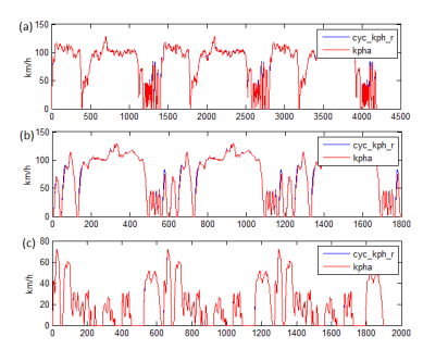
The first simulations were made for two built-in routes (CYC_REP05, CYC_US06) and the route for the agglomeration of Lodz developed by the author (CYC_LODZ). The acquisition of this route was made using parameters read from the vehicle’s OBD interface, and the ride was made during rush hour. Route speed profiles are shown in Fig. 5. To extend the travel time, the cycle was repeated three times. An example of the simulation result in the ADVISOR environment for transit using the built-in Toyota Prius model is shown in Fig. 6. The same initial conditions were used for all tests: SOC=0,7; SOC2=0,7; temp=20°C.
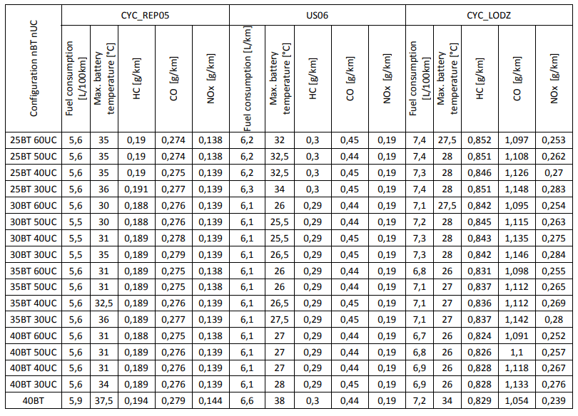
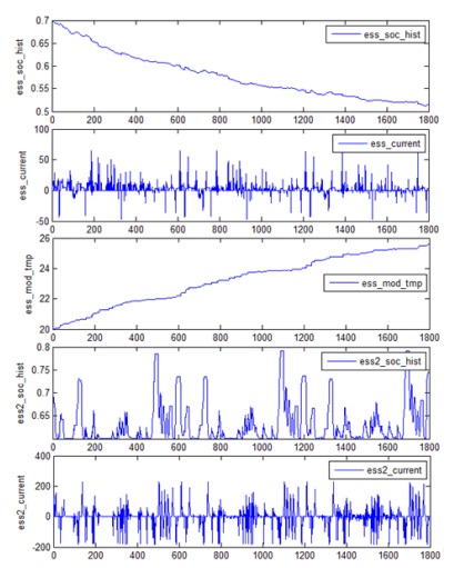
Then a series of simulations was performed using a modified version of the vehicle with an additional energy storage in the form of a supercapacitors package (30-60 modules) using the model embedded in the ADVISOR environment and a modified energy management system as described in chapter 3. An example of the simulation result is shown in Fig. 7. The rest of the simulation results for all routes in different combinations of the number of battery modules and supercapacitors (nBT and nUC where n is the number of modules, BT – baterries, UC – supercapacitors ) are shown in Table 2. 40BT refers to the original Toyota Prius.
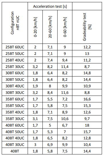
Additionally, for each nBT nUC configuration, perform an acceleration test and gradeability test at 50 km/h, at initial values SOC=0,6 and SOC2=0,6. The simulation results are shown in Table 1.
Table 1. The results of the acceleration and gradeability test
.
Table 2. Simulation results for the route CYC_REP05, CYC_US06 and CYC_LODZ
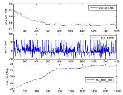
Fig.6. Simulation results for the route CYC_US06 (original Toyota Prius)
Fig.7. Simulation results for the route CYC_US06 for configuration 30BT 40UC
Conclusions
The simulation results show that the use of an additional energy storage in the form of a supercapacitor brings, in most cases, many benefits. First of all, in many cases lower fuel consumption has been achieved, which reduces the release of harmful substances by the vehicle. In addition, the use of an additional energy storage(supercapacitor) has reduced the number of battery modules (from standard 40 to 30-35). Less batteries means lower replacement costs when old batteries degrade. The proposed energy management strategy has reduced the average operating temperature of the battery pack, average current drawn from the battery, and on and off cycles, which has a positive effect on extending the life cycle of this energy storage. Adding an additional energy storage in the form of supercapacitors is associated with additional costs, but due to longer life and susceptibility to a large number of charging and discharging cycles (up to 1000000) this investment is a one-off with a typical vehicle life. The big advantage of supercapacitors, unlike batteries, is the ability to receive and release large amounts of energy in a short time, which is included in the proposed control strategy.
REFERENCES
[1] Bosch R., Napędy hybrydowe, ogniwa paliwowe i paliwa alternatywne, WKŁ, 2010 [2] Kouchachvili L., Yaici W., Entchev E., Hybrid battery/supercapacitor energy storage system for the electric vehicles, Journal of Power Sources, 374 (2018), 237-248 [3] Jaroszyński L., Akumulatory litowe w pojazdach elektrycznych, Przegląd Elektrotechniczny, 87 (2011), nr.8, 280-283 [4] Czerwiński A., Akumulatory, Baterie, Ogniwa, WŁK, 2005 [5] King A. , Power-hungry Tesla picks up supercapacitor maker, ChemistryWorld, 2019, https://www.chemistryworld.com/news/power-hungry-teslapicks-up-supercapacitor-maker-/3010215.article [6] Juda Z., Zastosowanie superkondensatorów w układzie odzysku energii pojazdu z napędem elektrycznym, Czasopismo Techniczne. Mechanika, 105 (2008), z. 6-M, 191-199 [7] Kasprzyk L., Bednarek K., Dobór hybrydowego zasobnika energii do pojazdu elektrycznego, Przegląd Elektrotechniczny, 91 (2015), nr.12, 129-132 [8] http://adv-vehicle-sim.sourceforge.net/ [9] Chen D., et al., ‘Research on Simulation of the Hybrid Electric Vehicle Based on Software ADVISOR, Sensors & Transducers Journal, 171 (2014), 68-77 [10] Gao D. W., Mi C. , Emadi A., Modeling and Simulation of Electric and Hybrid Vehicles, in Proceedings of the IEEE, 95 (2007), 729-745 [11] Rashid M. I. M., Daniyal H., Mohamed D.I, ‘Comparison performance of split plug-in hybrid electric vehicle and hybrid electric vehicle using ADVISOR’, MATEC Web Conf., 90 (2017), https://doi.org/10.1051/matecconf/20179001019 [12] Szumska E, Pawełczyk M., Ocena korzyści zastosowania napędów hybrydowych w pojazdach komunikacji miejskiej, Autobusy: technika, eksploatacja, systemy transportowe, 18 (2017), 1087-1092 [13] Wu Y., Power Distribution System Modeling and Simulation of an Alternative Energy, 2010, https://etd.ohiolink.edu/!etd.send_file?accession=ohiou1289960977&disposition=inline
Author: mgr inż. Piotr Woźniak, Politechnika Łódzka, Instytut Systemów Inżynierii Elektrycznej, ul. Stefanowskiego 18/22, 90-924 Łódź, E-mail: piotr.wozniak@dokt.p.lodz.pl.
Source & Publisher Item Identifier: PRZEGLĄD ELEKTROTECHNICZNY, ISSN 0033-2097, R. 96 NR 8/2020. doi:10.15199/48.2020.08.12
Published by Piotr ZEGARMISTRZ, Bartłomiej GARDA, AGH University of Science and Technology
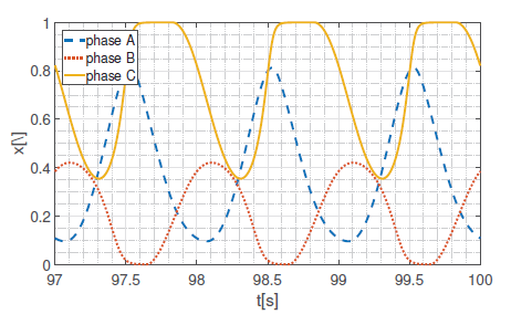
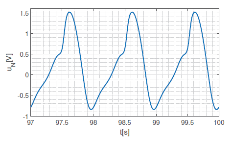
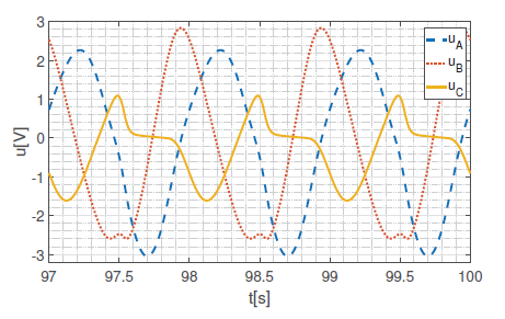
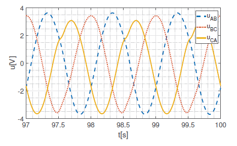
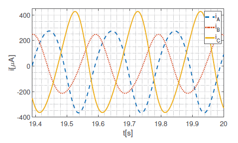
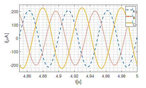
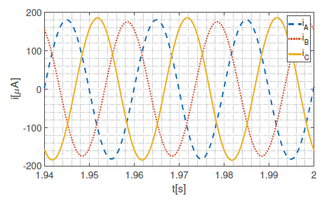
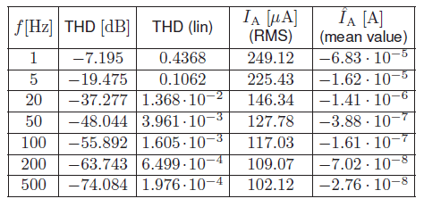
Abstract. The aim of the research presented in a paper was to provide trustworthy simulation results for symmetrical three-phase systems with memristive load. The memristors in the system are combined with linear resistors in order to limit the current in the element. Linear drift model of the memristor was considered in Matlab simulations. It is based on Strukov model with Biolek window. High nonlinearity of memristor results in deformation of most of the signals in the system. Since the voltage of the neutral point is highly non-sinusoidal it affects on other signals like phase voltage, phase currents, delta voltages. A Fast Fourier Transform (FFT) is applied to chosen signals in order to provide a frequency spectrum. On this basis a Total Harmonic Distortion (THD) parameter was calculated.
Streszczenie. W pracy zaprezentowano wyniki badan´ symulacyjnych nad układem trójfazowym symetrycznym z obcia˛z˙eniem elementami memrystorowymi. Memrystory w obwodzie odbiornika sa˛ poła˛czone szeregowo z rezystorami liniowymi w celu ograniczenia pra˛du. W obliczeniach symulacyjnych przyje˛ to model memrystora “linear drift”, bazuja˛cy na modelu Strukova z oknem Biolka. Wysoka nieliniowos´c´ elementów memrystorowych skutkuje odkształceniem wie˛kszos´ci sygnałów w obwodzie. Skoro napie˛cie punktu neutralnego odbiornika wykazuje wysoka˛ nieliniowos´c´, to skutkuje to odkształceniem pozostałych sygnałów, t.j. napie˛c´ fazowych, pra˛dów fazowych czy napie˛c´ przewodowych. Do wybranych sygnałów zastosowano Szybka˛ Transformate˛ Fouriera (FTT) w celu zaprezentowania widma cze˛stotliwos´ciowego. Na tej podstawie obliczono Współczynnik Zawartos´ci Harmonicznych. (Elementy memrystorowe w układach trójfazowych)
Keywords: memristor, memristive device, memristive element, three-phase systems, nonlinear systems Słowa kluczowe: memrystor, element memrystorowy, układy trójfazowe, obwody nieliniowe
Introduction
Theoretical definition of memristor was stated by L.O. Chua in 1971 [1][2]. It was defined as an element in which the actual value of resistance depends on the flux or charge through the element. It is capable of switching between two resistance states upon application of an appropriate voltage or current signal that can be sensed by applying a relatively much smaller sensing signal [3]. It was announced as the missing fourth fundamental passive circuit element.
In 2008 HP Laboratories reported the discovery of the element, which exhibits electrically controllable state dependent resistance [3][4]. It was a turning point in research on memristive devices. This topic became a priority for many R&D units and academic researchers. The most crucial property of memristor is the fact, that it can take two significantly different values of resistance in a stable way. This explains, why after 2008 this topic became so popular for scientists specializing in electronics, in particular memories, logic circuits and neuromorphic systems [5].
However, the applications of memrsitive devices focuses on microelectronics, that is not the one and only correct direction. In recent years the concept of so-called ’power memristor’ grows. The idea is to use memristive elements in lightning protection systems, i.e. instead of traditional varistors. In [6] author proposes a combined over-voltage protecting device consisting of a memristor connected in series with a spark gap. The memristor is applied for dissipating lightning surge energy and for breaking the short circuit current. This simple example shows, that analyzing the usage of memristive device in three-phase systems is noteworthy and can deliver a basis for further research.
A characteristic pinched hystersis loop (so-called bowtie curve) in v-i relation when applying a sinusoidal voltage to the element is also a special mark for memristors. This v-i histeresis loop always passes through the origin for any bipolar periodic input voltage [7]. The shape of the curve narrows down signifficantly with the frequency f. Beyond a certain critical frequency, the area of the loop decreases monotonically. It aims to zero with the frequency f increasing [8]. In this work, the authors decided to analyze the possibility of a usage of two-terminal memristive devices in threephase systems. It is assumed, that the system is powered by symmetrical three-phase source (i.e. set of three sinusoidal voltage sources with the same amplitude and phase shifted by 2π/3 ) and it is loaded by serial connection of a memristor and linear resistor with the value appropriate to limit the current in the memristive element in such a way that it is set in its work area. The basic aim of this study was to deliver a trustworthy information about the behavior of the signals in a three-phase system when memristive devices occur. To simplify the case study, it is limited to the symmetrical load version. The next aim was to analyze the impact of increasing frequency f of the input signal on the signals in the system.
Linear Ion Drift Model
This model is also known as Strukov model. It is assumed, that oxygen ions drift through the memristor structure with the velocity that depends linearly on the electric field. The v-i (voltage-current) relation in this model is:
.
where M{x(t)} = Ronx(t)+Roff(1−x(t)) represents the memristance of the memristive element in Ohms.
The internal variable x(t) denotes the relative width of the low-resistance region. Its dynamics is defined by the following formula:
.
To ensure that internal variable x(t) is confined to the interval [0, 1] one can multiply the right hand side of the equation above (2) by the ideal rectangular window function defined as f(x) = 1 for x ∈ [0, 1] and f(x) = 0 for others.
The above model depends on three parameters. Ron and Roff are the minimal and maximal resistances of the element, while the parameter k represents material properties and geometrical structure of the element.
Biolek Window Function
The equation (2) defining the elements dynamics does not take into account the physical phenomenon that switching mechanism is slower while states variable is close to the border of the limiting interval. One of the method that introduces this phenomenon is the window function application.
Then the equation (2) becomes:
.
where the f(x, i) is the mentioned window function of internal variable x and current i across the element. One of the popular window function is proposed by Biolek et al. [9], where the function f(x, i) is defined as:
.
where p is an even integer and 1 (·) represents a unit step function.
In this work a modified version of Biolek window is used, in which the absolute value of the expression under the power p is taken [10]. This permits using odd values of p also. Than, the Strukov model with the Biolek window is defined as:
.
The window function (4) introduces an additional integer parameter p to the Strukov model.
Simulations
All the simulations, results of which are presented in section below, were carried out in Matlab environment. Prepared simulation software gives the opportunity to measure and plot all of the signals in three-phase system, ie. voltage of the neutral point, phase voltages, phase currents, delta voltages and neutral wire current. It is possible to simulate both three-cord and four-cord systems, but in this paper only results for three-cord system are presented. The diagram of the circuit considered in the simulations is shown on Fig. 1. User can also set the specific value of phase wire resistance, as well as neutral wires resistances for four-cord case. Simulations for non-symmetrical loads, as well as for non-symmetrical three-phase sources are also possible. One can set an amplitude and phase shift for each phase voltage source separately. But this opportunity is not taken into account in this paper.
Fig.1. Diagram of the circuit considered in the simulations.
Results of the simulations for different frequencies are described in section below. For all simulations Linear Ion Drift Model with Biolek Window was used. This model bases on phenomena, that take place in real memristive element, so it is the most appropriate for that experiments.
Results
The main goal of the experiments was to show, how theoretically symmetric three-phase system behaves in terms of existing non-linear memristive elements. The simulations were made for the input phase voltages with RMS value 4V and linear resistance 1kΩ in series to memristor in order to limit the current in the element the same way, like in real measurements.
Fig.2. Internal variable x for memristors in phases A, B and C. Input signal frequency f = 1Hz.
Fig.3. Neutral point voltage. Input signal frequency f = 1Hz
Fig.4. Phase currents. Input signal frequency f = 1Hz.
Fig.5. Phase voltages. Input signal frequency f = 1Hz.
In this paper we focus on experiments made for the three-cord system. The frequency of input signals varies from 1 Hz to 500 Hz. Fig. 2 to 7 present the output parameters of the system for the frequency 1 Hz. To reduce the influence of the initial parameters all time series presented in the article shows the results of the simulation after some time of evaluation.
Shape of the internal variable x impacts on actual value of the resistance of memristor. This causes high non-linearity, which reveals in the shape of neutral point voltage signal. Since it is non-sinusoidal, all other signals in the system are non-sinusoidal. It is not obvious to find any conclusions for that results, but surely one can observe, that signals of the phase B are deformed in least significant way. This is confirmed in the shape of v-i curve (hysteresis loop), which is less pinched for phase B, than for the others. It is interesting that this phenomenon does not depend on different initial states values.
Fig.6. Time series of delta voltages for input signal frequency f = 1 Hz.
Fig.7. Hysteresis loop for phase voltages and currents for input signal frequency f = 1Hz.
Delta voltages (line voltages) are measured between connection nodes of linear resistor and memristor in each phase. Clearly, they are less deformed than other signals. An interesting observation may occur, when analyzing a frequency spectrum of the reported signals. In order to achieve it, the authors propose to perform a FFT (Fast Fourier Transform) on the signals. An answer of FFT for a chosen signal (phase A current) is shown on Fig. 8. It is important to notice the DC factor which value is on the level of second harmonic frequency. As it was mentioned earlier, the experiments were lead for wider range of frequencies.
As it is impossible to present graphs for all measured signals, authors decided to compare only chosen signals for higher frequencies – phase currents and v − i relation.
As one can see, the higher frequency, the more linear behavior of the memristive element. For frequencies 100 Hz and higher, the system behaved like fully linear system, so presenting graphs for them seems to be pointless. The general rule observed is, that the shape of the pinched hysteresis loop narrows down with increasing the frequency. For frequencies 500 Hz and higher it is straight line, so the memristor behaves as regular linear resistor.
Fig.8. Fast Fourier Transform of iA(t) current for input signal frequency f = 1Hz.
Fig.9. Time series of the phase currents for input signal frequency f = 5Hz.
Fig.10. Hysteresis loop for phase voltages and currents for input signal frequency f = 5Hz.
Conclusions
The authors performed also simulation results for four-cord systems, but because of limited space, it will be published in separate paper in near future. Presented results confirm the theoretical evidence, that memristor v − i characteristic tends to linear with increasing frequency. Moreover, for lower frequencies high non-linearity is observed. It motivated the authors to calculate a Total Harmonic Distortion (THD) parameter for chosen signals in order to show the degree of deformation of the signal versus frequency. In Tab. 1 the results for phase current iA are presented. Furthermore Tab. 1 contains RMS and mean values of iA. It is worth to notice that for low frequency f = 1Hz the value of the current is ca. 2.5 times higher than for the higher frequency f = 500 Hz. Also interesting is the fact of presence of DC factor which also tends to zero when the frequency increases.
Fig.11. Time series of phase currents for input signal frequency f = 20Hz.
Fig.12. Hysteresis loop for phase voltages and currents for input signal frequency f = 20Hz.
Fig.13. Time series of the phase currents for input signal frequency f = 50Hz.
In future work the measurements on real three-phase systems with memristive load is planned. Experimental research is the natural way to verify the results of analytical simulations. In order to achieve this a precise phase-shifting module needs to be design and build.
Fig.14. Hysteresis loop for phase voltages and currents for input signal frequency f = 50Hz.
Table 1. Basic parameters of phase A current iA vs frequency f
.
Acknowledgment: This work was supported by the National Science Centre, Poland, grant no. 2015/17/B/ST7/03763.
REFERENCES
[1] Chua L. O.: Memristor. The missing circuit element, IEEE Trans. Circ. Theory, vol. 18, no. 5, pp. 507–519, 1971. [2] Chua L. O.: The fourth element, Proc. IEEE, vol. 100, no. 6, pp.1920–1927, 2012. [3] Gandhi G., Aggarwal V., Chua L. O.: The first radios were made using memristors!, IEEE Circuits and Systems, vol. 13, no. 2, pp. 8–16, 2013. [4] Strukov D., Snider G., Steward D., Williams R.,: The missing memristor found, Nature, vol. 453, no. 7191, pp. 80–83, 2008. [5] Sacchetto D., Gaillardon P.-E., Zervas M., Carrara S., De Micheli G., Leblebici Y.: Applications of Multi-Terminal Memristive Devices: A Review, IEEE Circuits and Systems, vol. 13, no. 2, pp. 23–41, 2013. [6] Horváth I.: Simulation of a memristor-spark-gap model for lightning protection purposes, Tehnicki Vjesnik, vol. 21 (5), pp.1047–1050, 2014. [7] Pickett M., Strukov D., Borghetti J., Yang J., Snider G., Stewart D., Williams R.: Switching dynamics in titanium dioxide memristive devices, Journal of Applied Physics, vol. 106, 074508, 2009. [8] Adhikari S., Sah P., Kim, H.,Chua L.O.: Three fingerprints of memristor, IEEE Trans. on Circ. and Syst. I: Regular Papers, vol. 60, no. 11, pp.3008–3021, 2013. [9] Biolek Z., Biolek D., Biolkova B.: Spice model of memristor with nonlinear dopant drift, Radio Eng., vol. 18, no. 2, pp. 786–790, 2015. [10] Garda B., Galias Z.: Modelling sinusoidally driven selfdirected channel memristors, Proc. ICSES 2018, Cracow, Poland, pp.19–22, 2018.
Authors: Ph.D. Piotr Zegarmistrz, Ph.D. Bartłomiej Garda, Department of Electrical and Power Engineering, Faculty of Electrical Engineering, Automatics, Computer Science and Biomedical Engineering AGH University of Science and Technology, al. Mickiewicza 30, 30-059 Kraków, Poland, email: pzegar@agh.edu.pl; bgarda@agh.edu.pl
Source & Publisher Item Identifier: PRZEGLA˛D ELEKTROTECHNICZNY, ISSN 0033-2097, R. 96 NR 1/2020. doi:10.15199/48.2020.01.03
Published by MEKKAOUI Ali1, LAOUER Mohammed2, YOUNES Mimoun1, University of Sidi Belabes, Algeria (1), University Center of Naama, Algeria (2)
Abstract. Smart grids are essentially characterized by reliability and energy efficiency so we can optimize the performance of the electrical system to ensure safe and reliable operation. This paper discusses smart grids in a future generation context and to value this goal, we consider a new model of hybrid system combining solar and wind energy. In order to automate and ensure a wide distribution of the transmission and distribution network we will consider the bidirectional transfer of electricity and information solution. Our task in this work is to envisage an electrical power system connected to different consumers who can themselves produce electrical energy. Renewable energies will be present both at the level of the network in general and the subscribers which will allow a power exchange between the different actors.
Streszczenie. W artykule analizowano sieć typu smart grid nowej generacji będącą hybrydą energi fotowoltaicznej i wiatrowej. Uwzględniono możliwość dwukierunkowego transferu energii. Uwzględniono też różne typy odbiorców, w tym także tych wytwarzających energię. (Wymiana mocy w sieci typu smart grid z odnawialnymi źródłami energii)
Keywords: Active power, Renewable energy, Smart grids, Optimization. Słowa kluczowe: sieć typu smart grid, odnawialne źródła energii
Introduction
The limits of global fossil and nuclear fuel resources have prompted an urgent search for alternative sources of energy. Therefore, a new way to balance supply with demand is needed without the use of coal, gas or other generators. The smart grid will therefore play the role of an important system that will integrate renewable energy sources and move from dependence to fossil fuels, while respecting the balance of power produced and consumed.
The state of balance between production and consumption in current power systems must be checked at all times and in all places. Except that to be done, we will be in the obligation to control the transit of powers at any point of the network. The increased demand of power and the unexpected extension of the network disrupt the exchange of powers in real time. Is there a way to control, check and finally make the decision to ensure better management of electrical energy without there being a major failure? Otherwise, the system will be in a critical or even catastrophic situation. The answer to this question is implicitly given by using Smart Grids.
The Smart Grids provide the ideal solution to our problem, although they are a very interesting variant of energy saving. The conventional system must be modified because other components will appear and add to the existing power system to make it more complex and difficult to manage. The Smart Grids community relies on three different systems that provide unidirectional management from upstream to downstream. To know:
• The conventional and renewable energy generation systems, • The local system, • The transversal system.
The latter, is very important because it consists of active distribution networks and transport, controlled and adjusted in real time between supply and demand for energy.
The combination of these three systems is therefore the smart grid and responds to the priorities of the new electricity economy that can be summarized into three major conventional, renewable use values and the demand of the local system.
In addition, the following actions must be fully required:
• The integration of renewable and intermittent energies and new electrical uses, • The flexibility of production and consumption for the reduction of the electric tip, • Two-way flow of information and energy flows between the three system levels.
The future Smart Grid power grid is a dynamic network that aims at two-way power transit, largely linking small-scale renewable energy production systems at the consumer level and the larger electric power generation grid, thereby facilitating customer participation in energy management generation (consumption / consumption) in real time while raising the optimal performance of the operation of the power system [1]. Frequency and active power are the main parameters showing the stability of any conventional power grid [2]. The conventional power grid and computer and communication technologies are combined to control the active power flow to have a stable, reliable and efficient power grid.
Description and modelling of the hybrid system wind / solar
Regarding the wind system
Many studies have reported on this system and in particular the wind turbines [3]. The wind turbine model selected considers the characteristics of the wind speed as a function of the power output. The latter is given by [4- 5]:
.
where Pm is the mechanical output power of the turbine, Cp is the performance coefficient of the turbine, λ is the tip speed ratio of the rotor blade, β is the blade pitch angle, ρ is the air density, A is the turbine swept area and Vwind is the wind speed.
The model of performance coefficient Cp (λ,β) is taken from [4] and given by:
.
Where: constants C1to C6are the parameters that depend on the wind turbine rotor and the blade design, λiis a parameter given in (3).
.
So, Equality (1) can be normalized and simplified for specific values A of λ and as in (4):
.
where Pm_ pu is the power in per unit of nominal power for particular values A of λ , Vwind _ pu is the power gain of the base wind speed and Cp _ pu is the performance coefficient.
The based wind speed is the mean value of the expected wind speed in m/s .
Regarding photovoltaic system
For more than 30 years [6], the model of the photovoltaic system recommended is to consider the circuit consisting of a photo-current, a diode, a parallel resistance (leakage current) and a series resistance; the assembly is represented in Fig. 1. By applying Kirchhoff laws on the circuit, we can deduce the voltaic current which is given by [7]:
.
where Ipv is the photovoltaic current, IGC is the light generated current, Io is the dark saturation current dependent on the cell temperature, e is the electric charge e = 1.6*10-19C , Vdis the diode voltage, K is the Boltzmann’s constant K = 1.38*10-23J/K , F is the cell idealizing factor, Tcis the cell’s absolute temperature, Rp is the parallel resistance.
Knowing, on the other hand, that the photo-current depends essentially on the solar irradiation and the temperature of the cell, given by [7].
Fig.1. Single diode PV cell equivalent circuit.
.
where μsc is the temperature coefficient of the cell’s short circuit current, Tr is the cell’s reference temperature, Isc is the cell’s short circuit current at a 25oC and 1KW/m2 , G is the solar irradiation in KW/m2 .
Furthermore, the cell’s saturation current varies (Io) with the cell temperature, which is described as [6]:
.
.
where Ioα is the cell’s reverse saturation current at a solar radiation and reference temperature, Vg is the band-gap energy of the semiconductor used in the cell and Voc is the cells open circuit voltage.
Intelligent energy management systems
When a network has the capacity to effectively manage the actions undertaken by all the actors involved in the exchange of electrical powers (producers / consumers) and to ensure at the best of times a competitive electricity price, will talk about the smart grid. The main objective to achieve is to have low losses and a better quality of electrical energy. Such a network must include a smart meter, a smart home, a city server, and main server [8- 9].
Smart metering
The smart meter is the important component in the smart grids [10]; it consists of a bidirectional telecommunication subsystem to an information tele collection center. Its construction technology permits automatically to collect diagnostic data, consumption, available energy metering and transfer of this data to a central database [11].
Town server
For better management of electrical energy, the smart grids must be equipped with a city server. It will now have the ability to make any decision concerning all of its users through a central computer. To communicate with the primary server, it uses the public telephone network energy. It consists of a central computer and a complete server, capable of making decisions for all its users. It uses the public switched telephone network to communicate with the main server [12- 13].
Main server
It communicates in bidirectional way with smart home meters. Once the data is collected, It must be processed to validate it and finally stored in a central database [14- 15].
Analysis and control of active power
The collection of the energy consumption information of a smart home by the smart meter is sent to the command and control center [16]. The data generated by the smart meter is transmitted to a data aggregation. This aggregator could be an access point or gateway. The public electricity service or the distribution station and the intelligent communication is responsible for the transmission of the collected data. Fig. 2.
Fig.2. Power and information exchange in a smart grid
We can illustrate our study from a global diagram showing the different elements of a smart grid involved in the exchange of electric powers, as shown in Fig.3.
Fig.3. Flow chart of smart system.
Results and discussion
Our goal is to consider an electrical power system connected to the different consumers who themselves can generate electrical power. Renewable energies will be present both at the level of the network in general and the subscribers.
Fig.4. First house simulation results
The 24-hour extended load curve of house 1 is described in Fig. 4 (red color). The power exchange with the outside is represented by the residual power curve resulting from the difference between the power delivered by the wind turbine of the house 1 of the order of 4 kW and its power consumption (green color). Based on simulation results, we note the following situations:
• Between 00 h 00 and 06h 00 the house1 consumes a power of 0.5 KW, remains autumn and gives a residual power of 3.5KW to the electrical grid.
• A first peak appears around 6:00 am until 8:00 am reaches a value of 3KW; the house 1 is still isolated and provides the power grid with a power surplus of 1KW.
• Between 08h00 and 12h:00 the house consumes a power of 1KW and injects to the electrical system a surplus power of 3KW.
• A second peak reappears around 12:00 pm until 02:00 pm reaching a value of 2KW which reduces the surplus power to 2KW. The latter increases and holds a value of 3KW between 02:00 pm and 7:00 pm.
• A third bigger peak appears around 7:00 pm until 23h: 00 reaching a value of 5KW thus exceeding the production capacity of house 1. The difference is ensured by the electrical grid.
Fig.5. Second house simulation results
The exchange of electrical power between house 1 and house 2 is possible because house 1 has a residue of power. The charging curve of house 2 is in red, the power delivered by the house 1 is in green and the additional power supplied by the electric network in blue.
Based on simulation results, we note the following situations in Fig. 5:
• Between 00h00 and 08h:00 the house 2 consumes a power of 1KW provided by the house 1 thus reducing the surplus of the house 1 the remainder of which is made available to the need.
• At 8:00 am the consumption of house 2 increases and reaches a value of the order of 2KW which will always be powered by the house 1.
• A peak consumption is observed at 19h00 until 23h: 00 which involves the power grid to satisfy the electrical energy demand of the house 2.
Fig.6. Third house simulation results
The extended load curve over 24 hours of the house 3 is given by Fig. 6 in red color. The power exchange with the outside is represented by the residual power curve (in green color) which results from the difference between the power delivered by the solar energy of 4KW and the power consumed by the house 3. According to The results of simulations, we note the following situations:
• Between 00:00 and 06:00 in the morning house 3 consumes a power of 0.5 KW which is delivered by the electricity grid.
• The presence of the first peak from 06h: 00 to 08h00 of the order of 3KW is ensured by the electricity grid.
• The sun makes its appearance from 08h 00, at this moment the house 3 consumes a power of 1KW which will be delivered by its solar energy. Then house 3 remains autumn and gives a residual power of 3KW until 19h: 00.
• A second consumption peak of 6KW is observed from 20h 00 until 23h00, which involves the power grid to satisfy the energy demand of the house 3.
Fig.7. Fourth house simulation results
Fig. 7 shows the load curve (red color), the curve of the solar energy produced by the house 3 (green color) and finally the curve of the electricity network (blue color).
Based on simulation results, we note the following situations:
• Between 00h00 and 06h: 00 the house 4 consumes a power of 1KW which is delivered by the electrical network.
• A first peak appears from 06h00 to 08h:00 reaching a value of 4KW but always ensured by the electricity grid.
• From 08:00 to 19:00 the house 4 is fueled by the energy coming from the house 3 despite the presence of the second peak of consumption which is of the order of 3 KW.
• A third peak of consumption is observed at 20:00 until 23:00 which of the order of 6KW this energy is supplied by the electrical network.
Conclusion
It is very interesting to understand the transfer and the exchange of electrical energy between the different actors participating in this action. This article clearly explains the integration of renewable energies into the conventional electricity grid for better and intelligent management of home energy. The simulation of such a system consisting of houses and the existing electricity network has provided the answer, so long awaited, explaining the interest brought by the smart grid. Our simulation clearly explains the contribution of the houses in the network stability in the sense of its relief in case of the strong demand. Thus, we can conclude that smart grids offer a radical solution to the reliable and continuous operation of the entire system.
Authors, Ali Mekkaoui, Pr. Younes Mimoune, University of Sidi Belabes, Algeria and Pr. Mohammed Laouer, University Center of Naama, Algeria, Email: mekkaouiali70@gmail.com, younesmi@yahoo.fr laouer@yahoo.fr
Source & Publisher Item Identifier: PRZEGLĄD ELEKTROTECHNICZNY, ISSN 0033-2097, R. 96 NR 12/2020. doi:10.15199/48.2020.12.17
Published by Małgorzata ŁATKA, Marek NOWAK, Rzeszow University of Technology
Abstract. The article presents the results of a comparative analysis of the basic indicators characterizing the interruptions in the supply of electricity. On the basis of generally available reports of selected DSOs, a list of selected indicators was prepared over the years. A comparison of these data was made, for the largest energy distribution companies in Poland. Conclusions from this analysis may be used to determine the level of power supply reliability and energy security of the country.
Streszczenie. W artykule przedstawiono wyniki analizy porównawczej podstawowych wskaźników charakteryzujących przerwy w dostawach energii elektrycznej. Na podstawie ogólnie dostępnych raportów wybranych OSD opracowano zestawienia wybranych wskaźników na przestrzeni lat. Dokonano porównania tych danych, dla największych spółek dystrybucyjnych w Polsce. Wnioski z tej analizy mogą być wykorzystane do określenia poziomu niezawodności dostaw energii elektrycznej i bezpieczeństwa energetycznego kraju. (Analiza porównawcza wskaźników dotyczących przerw w dostawach energii elektrycznej dla odbiorców energii elektrycznej dla wybranych operatorów systemów dystrybucji)
Keywords: SAIDI, SAIFI, MAIFI, power supply breaks, comparative analysis Słowa kluczowe: SAIDI, SAIFI, MAIFI, przerwy w zasilaniu, analiza porównawcza.
Introduction
Companies that are involved in the distribution of electricity are obliged to provide information to their customers, regulated by relevant regulations. Distributors, in the form of annual reports, provide information on the number of interruptions and their length, i.e. indicators of the duration of interruptions in the supply of electricity. Interruption duration indicators are SAIDI, SAIFI and MAIFI for example. These indicators show the average length of long breaks, the average number of breaks and the average number of short breaks per consumer. In addition to these three, there are a number of other indicators. The improvement of these indicators is in the interest of energy distributors and is the subject of research by many scientific teams. [1÷6]
In terms of the area of electricity distribution, the territory of Poland was divided among 5 large DSO Distribution System Operators. There are also small companies dealing with the distribution of electricity, serving a much smaller number of customers. They are also obliged to provide information on selected indicators.
The article presents the results of a comparative analysis of selected indicators characterizing the size of power supply interruptions for various distributors operating in Poland. The comparative analysis of indicators was carried out on the basis of generally available data on the Internet and on the basis of detailed information obtained directly from operators. A number of aspects have been taken into account, such as: the length and types of power lines, the amount of transmitted energy, the amount of investment funds, the multi-year time space, the division of indicators taking into account the types of interruptions. The results of the analysis were presented both in tabular and graphical form on charts, which constituted the basis for the formulation of final conclusions.
Energy security
One of the basic concepts inherent in energy quality is energy security. On the basis of the Energy Law Act, energy security can be defined as a state in which the economy is able to fulfill the demand (current and predicted) of consumers for energy (electricity, gas, fuels) in a technically and economically justified manner, taking into account environmental considerations. As can be seen from the above definition, the power system must be characterized primarily by the continuity of electricity supply, and the power company is obliged to provide it. These obligations result from Article 9 of the Energy Law Act, which contains the requirements that are imposed on the energy company, and these are:
• to generate electricity or to be prepared to generate it; • having a power reserve; • the ability of energy sources to produce energy in the amount resulting from the concluded agreements; • informing the power system operators about the condition of the generation equipment.
The notion of continuity of electricity supply is also associated with a state in which such continuity is not ensured. Such a period is called a power outage. Consumers expect power cuts to be as short and rare as possible, while maintaining a low electricity price.
These issues are the subject of constant discussion, which is due, inter alia, to the fact that depending on the type of customer (whether they are utilities or industrial customers), the requirements for continuity of energy supply vary.
Electricity supply interruption indicators
The main electricity quality indicators associated with power outages are: SAIDI, SAIFI and MAIFI. These indicators are also provided in the annual reports prepared by electricity distribution companies.
SAIDI (System Average Interruption Duration Index) – indicator of the average system duration of a long interruption in electricity supply, expressed in minutes per customer
.
where: Ui – annual time of the i-th break, Ni – number of customers affected by the break, NT– the total number of customers.
SAIFI (System Average Interruption Frequency Index) – average frequency of long interruptions in energy supply. It does not include intervals of less than 3 minutes and shall be determined separately for planned and unplanned outages. It shall be given in the number of interruptions per customer:
.
where: λi– annual number of breaks planned or not planned, Ni– number of customers affected by the break, NT– the total number of customers.
MAIFI (Momentary Average Interruption Frequency Index) – average frequency of short interruptions in electricity supply. Calculated as the ratio of short interruptions to the number of consumers:
.
where: Ai– annual number of the short breaks, Ni – number of customers affected by the break, NT – the total number of customers.
Besides SAIFI, SAIDI, MAIFI, other indicators are used, such as ENS, AIT, ASAI, ASUI. All of them will be discussed below, as well as their calculation.
ENS (Energy Not Supplied) – is the value of energy not supplied to consumers as a result of interruptions:
.
where: Pi – power not delivered, Ui– duration of i-th break.
AIT (Average Interruption Time) is a measure of the time during which energy is not delivered to consumers:
.
where: ENSi – amount of the energy not delivered in i-th case, PT – average power delivered to the customers.
ASAI (Average Service Availability Index) – is the average time of availability of electricity supplies:
.
where: Ui– annual break time of the i-th customer, Ni– number of customers.
ASUI (Average Service Unavailability Index) – it is the average time of unavailability of electricity supplies:
.
where: Ui – annual break time of the i-th customer, Ni– number of customers.
The values of these indicators should be as small as possible, as this would indicate that there are no interruptions of electricity supply, or that they are negligible.
In addition to the basic indicators given, more detailed versions are also given, for example, those that take into account the type of gaps (planned, unplanned, etc.) or refer to economic indicators (e.g. GDP) and determine the losses incurred in the economy. These are e.g:
• SAIDI BK – SAIDI for unplanned breaks without catastrophic breaks • SAIDI P – SAIDI for planned breaks • SAIDI K – SAIDI for unplanned breaks with catastrophic breaks • SAIFI BK – SAIFI for unplanned breaks without catastrophic breaks • SAIFI P – SAIFI for planned breaks • SAIFI K – SAIFI for unplanned breaks with catastrophic breaks.
The electricity market in Poland
In Poland, there are five large distribution system operators whose number of customers ranges from 1 to approximately 5.5 million. The remaining DSOs provide services of a much smaller range. However, their market share is significant (about 25%). Therefore, it is important that both groups of DSOs supply electricity to their customers in an uninterrupted and continuous manner, which is confirmed by the lowest possible values of the discussed indicators. Table 1 presents data related to mentioned five DSOs and their customers. [7]
Table 1. Characteristics of large DSOs in Poland
.
SAIDI, SAIFI and MAIFI indicators for selected DSOs
Table 2 contains aggregate SAIDI data for both planned and unplanned (including catastrophic) disruptions for the 5 largest DSOs in Poland in 2012÷2018, which are graphically shown in Figure 1.
Table 2. SAIDI for the 5 largest DSOs in Poland over the period 2012÷2018 [7÷12]
.
The analysis of SAIDI data (Fig. 1) shows that for 4 operators (DSO1 to DSO4) the trend is decreasing, while for DSO5, the ratio remains constant, at the lowest level compared to other DSOs. While in the years 2012-2016, a steady decrease can be observed in DSOs1, DSOs2, DSOs3 and DSOs4, despite the downward trend, there are also increases in some years. The exception for almost all operators is 2017, when each of them (except for DSO5) recorded a significant increase in SAIDI. The year 2017 was full of rapid weather phenomena in Poland (e.g. Ksawery Orkney) [12]. Since the general SAIDI index (including planned and unplanned interruptions, including catastrophic ones) was taken into account, the atmospheric factor undoubtedly contributed significantly to the increase in this index.
Fig.1. SAIDI for DSOs in Poland over the period 2012÷2018.
This is confirmed by the analysis of the SAIDI for planned interruptions (fig. 2). In 2018, all operators recorded the lowest SAIDI values for the period under consideration.
Fig.2. SAIDI for planned breaks for DSOs in Poland (2012÷2018)
Another indicator analyzed is SAIFI for planned and unplanned (including catastrophic) interruptions. Table 3 contains aggregated operator data and Figure 3 illustrates this.
Table 3. SAIFI for the 5 largest DSOs in Poland over the period 2012÷2018 [7÷12]
.
Unlike SAIDI, SAIFI maintains a rather constant value with minor changes. It is difficult to determine the trend of changes in this indicator for the period 2012÷2018. Similarly to SAIDI, the indicator increased in 2017, but it was the maximum value in the audited period, only for DSOs1. It can be concluded that the number of interruptions varies slightly, but their length (SAIDI index) decreases, e.g. due to the use of new technologies during repairs and work under voltage, if possible.
The smallest values of SAIDI and SAIFI coefficients have a DSO5. It results from the fact that the operator operates in a much smaller area than the others and due to the specificity of this place (large city), cable lines have a much larger share in the infrastructure (nearly 87%). Due to the fact that the cable lines are effectively separated from the prevailing weather conditions, the operator is able to maintain the coefficients at such a low level.
Fig.3. SAIFI for DSOs in Poland over the period 2012÷2018.
Capital expenditures influence on SAIDI and SAIFI
Figures 8÷12 show the value of SAIDI index in relation to investment outlays of selected distribution system operators.
Distribution System Operators have been maintaining a rather stable level of investment since 2012, with the exception of DSO3, which decreased investments twice in 2013. It is difficult to find, however, a visible impact on the SAIDI indicator of the funds allocated for network modernization. However, it can be concluded that fixed capital expenditures are conducive to the decrease of this ratio.
Fig.8. SAIDI in relation to DSO1 investment outlays in 2012÷2017.
Fig.9. SAIDI in relation to DSO2 investment outlays in 2012÷2017.
Fig.10. SAIDI in relation to DSO3 investment outlays in 2012÷2017.
Fig.11. SAIDI in relation to DSO4 investment outlays in 2012÷2017.
Fig.12. SAIDI in relation to DSO5 investment outlays in 2012÷2017.
Summary
Electricity supply continuity indicators have an important role in the economy today. They make it possible to assess the quality of the service provided to the electricity consumer – securing the continuity of power supply. Their analysis makes it possible to determine whether the activities of distributors over the years have resulted in an improvement in supply conditions and to what extent it depends on the type of distributor.
In addition to indicators, DSOs also make available the amount of capital expenditures incurred. However, it is difficult to find any unambiguous positive impact on the indicators. Perhaps this is because the DSO, in order to reduce the unfavourable statistics, performs a lot of renovation or modernization works, but they are qualitatively questionable, which makes the durability of these investments much lower. SAIDI is also significantly affected by unplanned interruptions related to weather conditions and other damage.
A big disadvantage of the presented indicators is the exclusion of short breaks during their calculation, which from the point of view of the recipient are the most troublesome. Such short breaks often occur “one after the other”, which is particularly bad for large energy consumers, such as production plants.
REFERENCES
[1] Parol M., „Analiza poziomu niezawodności zasilania odbiorców w elektroenergetycznych sieciach dystrybucyjnych”, Przegląd Elektrotechniczny Nr 3/2017, pp. 1 – 6 [2] Olejnik B., Łowczowski K., „Techniczne metody poprawy współczynników SAIDI oraz SAIFI stosowane w sieci dystrybucyjnej”, Poznan University of Technology Academic Journals. Electrical Engineering Nr 86, 2016 pp. 165-176 [3] Halinka A., Niedopytalski M.,Rzepka P., Sowa P. and Szablicki M., “Expert evaluation method of the SAIDI normative reliability index,” 2015 Modern Electric Power Systems (MEPS), Wroclaw, 2015, pp. 1-4.. [4] E. van Schalkwyk, “The value of an incremental (mitigated) SAIDI minute,” 2010 20th Australasian Universities Power Engineering Conference, Christchurch, 2010, pp. 1-3. [5] M. Kruithof, J. Hodemaekers and R. Van Dijk, “Quantitative risk assessment; A key to cost-effective SAIFI and SAIDI reduction,” CIRED 2005 – 18th International Conference and Exhibition on Electricity Distribution, Turin, Italy, 2005, pp. 1-5. [6] V. Mariappan, A. B. S. M. Rayees and M. AlDahmi, “Earthing system analysis to improve protection system performance in distribution networks,” 12th IET International Conference on Developments in Power System Protection (DPSP 2014), Copenhagen, 2014, pp. 1-6. [7] PTPiREE, “Energetyka. Dystrybucja i Przesył” http://ptpiree.pl/documents/2019/raport_ptpiree_2018.pdf [8] https://pgedystrybucja.pl/ [9] https://www.tauron-dystrybucja.pl/ [10] https://www.energa-operator.pl/ [11] https://www.operator.enea.pl/ [12] https://www.innogy.pl/ [13] https://tvnmeteo.tvn24.pl/informacje-pogoda/polska,28/2017-year-w-pogodzie-zapamietamy-go-na-dlugo,249675,1,0.html
Authors: Małgorzata Łatka, PhD, Eng., Rzeszow University of Technology, Faculty of Electrical and Computer Engineering, W. Pola 2, 35-959 Rzeszów, E-mail: mlatka@prz.edu.pl; Marek Nowak MSc, Eng., Rzeszow University of Technology, Faculty of Electrical and Computer Engineering, W. Pola 2, 35-959 Rzeszów, E-mail: mnowak@prz.edu.pl;
Source & Publisher Item Identifier: PRZEGLĄD ELEKTROTECHNICZNY, ISSN 0033-2097, R. 96 NR 1/2020. doi:10.15199/48.2020.01.08
Published by Doh-Young PARK1, Jacek F. GIERAS2,3 Korea Institute of Machinery and Materials, Daejeon, Korea (1), UTP University of Science and Technology, Bydgoszcz, Poland (2), Korea Electrotechnology Research Institute, Changwon, Korea (3),
Abstract. The paper presents the Incheon Airport Maglev Line (IAML) in South Korea connecting Incheon Airport with Yeongjong Island. The paper focuses on construction of elevated track and infrastructure, magnetic levitation and propulsion, cars of trainset, power consumption and operating costs.
Streszczenie. W artykule przedstawiono kolej magnetyczną Incheon Airport Maglev Line (IAML) w Korei Płd. łączącą port lotniczy Incheon z wyspą Yeongiong. Szczególną uwagę zwrócono na konstrukcję toru umieszczonego na estakadzie, lewitację magnetyczną, napęd silnikami liniowymi, wagony, pobór mocy oraz koszty operacyjne. (Kolej magnetyczna Incheon Airport Maglev Line)
Keywords: maglev line, Incheon Airport, linear motors, power consumption, operating costs. Słowa kluczowe: kolej magnetyczna, port lotniczy Incheon, silniki liniowe, pobór mocy, koszty operacyjne.
Introduction
Korea Urban Maglev Program started in December 2006 at Korea Institute of Machinery and Materials (KIMM) in Daejeon. The construction of passenger carrying service of 6.1-km, low-speed Incheon Airport Maglev Line (IAML) started on February 3, 2016. It was preceded by complete and thorough system interface tests, part of which were required by the regulations.
The IAML is a completely passive system with attraction electromagnets and primary units of the linear induction motor (LIM) installed in vehicles, while reaction rails for electromagnets and LIMs are installed in the track [1].
The IAML connects Incheon International Airport Transportation Center (IIATC) with Yongyu station in Yeongjong Island. There are 6 stations: (1) IIATC, (2) LongTerm Parking, (3) Administration Complex, (4) International Business Center, (5) Water Park, (6) Yongyu Station.
Fig.1. Route map (red line) of the IAML.
Construction
The double-track elevated guideways of the IAML are installed on concrete pillars. The highest elevation is 24.5 m, the maximum gradient is 45 ‰ and the minimum curve radius 50 m. There is a maintenance depot and control center in the vicinity of Yongyu Station. The route map is shown in Fig. 1. The trainset on elevated guideway is shown in Fig. 2.
The Incheon Airport Transportation Center Station is shown in Fig.3. The travel is free of charge. The first maglev train leaves the IIATC at 7:30 and the last train at 20:15. The first train leaves the Yongyu Station at 7:31 and the last train at 20:01. The trains operate in 15 min intervals. The travelling time is 12 min. for 6.1-km trip. There are 103 trips per day
Fig.2. The maglev trainset on elevated guideway. Photo taken near maintenance depot (Yongyu Station).
Fig.3. The Incheon Int. Airport Transportation Center Station.
Fig.4. Top view of the IAML track.
The operator is the Airport Railroad Corporation. There are two tracks in parallel. The track gauge is 1850 mm (Fig. 4). The line is electrified at 1500V DC. The electric power is fed to the vehicle with the aid of two contact rails mounted at each side of the concrete elevation (Fig. 5). There are two sliding contacts per vehicle. The average speed is 30.5 km/h including stops at the stations, cruising speed is 80 km/h, and maximum speed is 110 km/h. Specification of IAML are given in Table 1 [1,2,3].
Table 1. Specification of IAML [1,2]
.
Fig.5. Contact power transfer to vehicles:
1 – sliding contact mounted in the bogie, 2 – contact rail, 3 – insulator.
The construction cost per 1 km was US$ 37.8 million in 2009 [2]. For comparison, the average cost per 1 km of light railway (wheel-on-rail), rubber tire shuttle or monorail in Korea was US$ 41.4 million in 2009 [2].
Magnetic levitation and propulsion
The IAML uses electromagnetic levitation (EML), i.e., attraction forces between electromagnets and reaction rails and LIM propulsion. The suspension and propulsion system is shown in Fig. 6.
Suspension electromagnets, which produce attraction force have steel core with U-cross-section. The nominal air gap between the electromagnets poles and steel reaction rail is 8 mm. The constant levitation gap is maintained by controlling the electric current fed to the windings of electromagnets with the aid of sensors and controllers. Fig.7 shows the car-mounted suspension electromagnet and part of the primary unit of the LIM mounted above the electromagnet. Both electromagnets and the primary units of LIMs are air cooled.
Stable levitation is maintained for at least 30s after power failure with the aid of the backup battery system, which is eco-friendly and easy to maintain. The steel rail for suspension electromagnets is also a part of the reaction rail (secondary unit sometimes called “back iron”) for the LIM (Fig. 6). To reduce the impedance of the reaction rail and improve all performance characteristics of the LIM, the active surface of the steel reaction rail is furnished with a high-conductivity plate. Copper is too expensive metal, so aluminum plate is used almost in all LIM-driven vehicles around the world. The IAML also uses aluminum plate on the active surface of the steel reaction, which is visible in Fig. 4. The nominal air gap (mechanical clearance) between the primary unit core of the LIM and aluminum plate is 13 mm. The LIM is fed from a VVVF inverter. There are four LIMs per each side of the car. Each LIM and four suspension electromagnets create a suspension-propulsion unit (Fig. 8).
Fig.6. Magnetic levitation and propulsion systems:
1 – steel core of suspension electromagnet, 2 – winding of electromagnet, 3 – suspension force, 4 – air gap sensor, 5 – steal reaction rail for suspension electromagnets and LIM, 6 – aluminium cap to reduce the resistance of reaction rail for LIM, 7 – primary unit of LIM, 8 – bracket for electromagnets (part of bogie), 9 – car body, 10 – base of the track (sleeper), 11 – concrete beam.
Fig.7. Suspension electromagnets:
1 – steel core of the electromagnet, 2 – coil of the electromagnet, 3 – three-phase winding of the primary unit of the LIM, 4 – bogie of the car, 5 – steel reaction rail for suspension electromagnet (part 5 of Fig. 6). Photo taken in the maintenance depot.
The are 4 propulsion LIMs installed at each side of the car, altogether 8 LIMs per car. Each LIM has 6 poles. LIMs are fed from VVVF inverters. LIMs are shown in Fig. 9. Propulsion system can provide maximum acceleration of 4.0 km/h/s and maximum deceleration of 4.5 km/h/s in the case of emergency. The empty weight of each vehicle is 19.5 tons and the full weight with passengers is 26.5 tons.
Fig.8. Suspension-propulsion unit:
1,2,3,4 – electromagnets, 5 – three-phase winding of the primary unit of the LIM. Photo taken in the maintenance depot.
Fig.9. LIMs for propulsion of IAML cars.
Cars
The design of the car body incorporates traditional Korean curvature and honeycomb pattern (Fig. 10). The lightweight car body has been made with the aid of single skin aluminum extrusion technology. Electro-hydraulic and pneumatic brake systems provide excellent braking performance. The lighting and illumination system is entirely composed of LEDs to save energy. Dimmed windows protect the privacy of neighbourhoods the trainset passes by. The dimming effect is the result of an electrified gel sandwiched between two thin pieces of glass. As the electric current increases, the gel darkens and as it drops, the gel lightens.
Fig. 10. Car body incorporates traditional Korean curvature and honeycomb pattern on both sides of the car (below windows).
Operating costs
Operating costs of IAML include [2,3]:
• employment cost; • electric power consumption cost; • maintenance cost; • administrative cost.
Electric power cost is the cost of electricity consumed by vehicles and general electric loads (Table 2). The maglev vehicle consumes electric power for propulsion, levitation, plugging (braking) and operation of service equipment. The general electric loads include lighting, fans, communication equipment, PA, and electricity consumed by buildings and stations for passenger service operation.
Maintenance cost consists of utility cost (electric power consumption), commission/service (outsourcing) cost, material cost, repair cost, train maintenance, communication charge and supplies expense. Administrative expense is generated by general management of the administration division. It includes insurance premiums, cost, and service charges for cleaning and security.
Breakdown of operating costs is given in Table 3. Salaries of employees contribute to almost 70% of the total costs.
Table 2. Annual Power Consumption [2]
.
Table 3. Breakdown of operating costs for IAML [2]
.
Conclusions
• The IAML is a low-speed EML passenger transportation system driven by LIMs with completely passive track. • The construction cost of 1 km of double-track line was US$ 37.8 million in 2009, i.e., 9.5% less than the construction of 1 km of traditional light railway. • The annual operating costs of IAML are about US$ 6.3 million.
REFERENCES
[1] ECOBEE: the cutting edge technology, Korea Institute of Machinery and Materials (KIMM), Daejon. [2] K. B. Lee, S. K. Ma,.B. C. Shin, D. Y. Park, Study of calculation of standard operating costs of Incheon Airport Maglev Line, Transportation Systems and Technology, 4 (2018), nr 1, 5-18. [3] D.Y. Park, B. C. Shin, H. Han, Korea’s Urban Maglev Program, Proc. of the IEEE, 97 (2009), nr. 11,
Authors: Dr inż. Doh Young Park, Korea Institute of Machinery and Materials (KIMM), Center for Urban Maglev Program, Daejeon, Korea, E-mail: dypark@kimm.re.kr ; prof. dr hab. inż. Jacek F. Gieras, IEEE Fellow, UTP University of Science and Technology, Dept of Electrical Engineering, Al S. Kaliskiego 7, 60-965 Bydgoszcz, Poland, E-mail: jacek.gieras@utp.edu.pl
Source & Publisher Item Identifier: PRZEGLĄD ELEKTROTECHNICZNY, ISSN 0033-2097, R. 95 NR 6/2019. doi:10.15199/48.2019.06.01
Published by Konrad DĄBAŁA1, Marian P. KAZMIERKOWSKI1,2, The Łukasiewicz Research Network – Electrotechnical Institute, Warsaw (1) Warsaw University of Technology, Faculty Electrical Engineering (2)
Abstract In this paper the basic requirements and current developments of converter-fed drives for electric vehicles, particularly for electric cars, are reviewed and compared. The basic parts of the powertrain have been presented in the following sequence: electric traction motors, power electronic converters and traction control methods. Possible future developments of this components are discussed and summarized.
Streszczenie W artykule omówiono i porównano podstawowe wymagania oraz aktualne rozwiązania napędów przekształtnikowych dla pojazdów elektrycznych, w szczególności dla samochodów elektrycznych. Podstawowe części układu napędowego przedstawiono w następującej kolejności: elektryczne silniki trakcyjne, przekształtniki energoelektroniczne i metody sterowania momentu i strumienia silników trakcyjnych. Zaprezentowano kierunki przyszłych zmian i tendencji rozwojowych poszczególnych części takich napędów. Omówienie i porównanie podstawowych wymagań oraz aktualnych rozwiązań napędów przekształtnikowych dla pojazdów elektrycznych
Keywords: Electric vehicles (EV), Electromobility, powertrain, traction motors, power electronics propulsion. Słowa kluczowe: Pojazdy elektryczne, Elektromobilność, napędy pojazdów, silniki trakcyjne, przekształtniki energoelektroniczne.
1. Introduction
Recently, the fast development of plug-in hybrid electric (PHEV) and battery electrical vehicles (BEV) is observed. This trend was accelerated by American Tesla Motors and currently is strongly continued by most of Asian (Toyota, Nissan, Honda, Hyundai) and European (VW, Renault, PSA, Audi, BMW) car producing companies [1]. Among most important advantages of BEV are:
• no exhaust, • low exploitation costs (compared to cars with combustion engines 1: 3), • high efficiency of electric motors > 90% (combustion engine 35-40%), • simple construction, no gearbox and clutch, • low noise, • energy recovering during braking and recharging the batteries from 5 to 20% (depending on the driving style), • further cost reduction charging batteries during periods of lower demand for electricity (at night and at noon).
However, despite of significant advances in BEV technology, there are still restrictions on their mass use. These include, above all:
• high price (about 30-50% higher than equivalent cars with combustion engine), • small range based on one battery charging, • long time of battery charging, • lack of developed battery charging infrastructure, •charging infrastructure requires production of an additional energy (power).
Many of these problems help to solve advanced and modern power electronics. Therefore, the Power Electronics systems has broadly entered Electromobility in the area that can be divided into three specific groups [1, 2, 3]: architecture of the power supply of charging station (in particular ultra-fast charging), battery charger systems themselves, and powertrain with AC motors. In this paper, due to the space limitation, we discuss only the powertrain systems for BEV. Typical components of a BEV powertrain are (Fig. 1): electric motor, power electronic system and traction control system. These components will be discussed below.
Fig. 1. Typical components of an EV powertrain
2. Electric traction motors
2.1 Types and characteristics
When analyzing the drives currently used (or will be used) in electric vehicles, particularly in BEV cars, one can conclude that they can be divided in three main groups: synchronous motors, induction motors, switched reluctance motors [1, 4, 11]. Synchronous and reluctance switched motors have various variants related to the construction and use of permanent magnets (Fig. 2).
Squirrel-cage induction motors (IM) (Fig. 3a) are machines with well-controlled technology and the introduction of rotors with copper casted cages increased their efficiency. Methods for determining the efficiency of induction motors are also developed and refined [5, 6, 7].
However, the IM have a lower power density (power/weight parameter) than the synchronous motors (SM) [2, 8].
Fig.2. Classification of motors used in electric vehicles. In the filled frames are motors discussed in this article
Synchronous motors with permanent magnets placed on the surface of the rotor (SPMSM) (Fig. 3b) have high efficiency due to practically zero losses in the rotor and less mass. Motor design should take into account the heat dissipation from the motor, so that the magnets do not work at too high temperature as they may be exposed to demagnetisation.
Synchronous motors with permanent magnets placed inside the rotor (IPMSM) (Fig. 3c) are characterized by high efficiency and the possibility of flux weakening to a limited extent. As in SPMSM, proper cooling of the motor should be ensured so as not to demagnetize of magnets.
Synchronous reluctance motors (SynRM) (Fig. 3d)) operate on the principle of using the reluctance torque present in the machine due to the difference of conductivity in the d-axis and the q-axis. The greater their difference, the greater the torque of the motor. These are motors in which there are no permanent magnets. They have high efficiency, but a large mass and low power factor [9].
Synchronous reluctance motors with permanent magnets (PMSynRM) (Fig. 3e) differ from the previous ones by additionally using permanent magnets in the rotor. It definitely improves the motor parameters, particularly its power factor.
Fig.3. Types of motors used in electric vehicle drives:
Switched reluctance motors (SRM) (Fig. 3f) are characterized by a very simple construction. The concentrated windings used in them, compared to the distributed windings (usually used in alternating current motors) allow to reduce the amount of copper and the mass of the motor. SRMs have high efficiency, but very high torque ripple, high levels of noise and vibration. The advantage of them is the possibility of continuing work even when there is no power supply for one phase.
Switched reluctance motors with permanent magnets (PMSRM) (Fig. 3g) placed in the stator have better parameters than SRM, less torque ripple, less noise and vibrations. Since the magnets are placed in the stator, cooling is easy. Hybrid excitation motors (HEPMSRM) are the variant of these motors, in which there is an additional excitation winding in the stator in addition to the armature winding and permanent magnets [10, 11]. Control is more complicated, but the motor’s parameters are better.
2.2 Price of rare-earth magnets
Motors that use rare-earth magnets (Fig. 3 (b), (c), (e), (g)) may be uncompetitive in relation to motors without such magnets, because of the magnets price. Fig. 4 (based on [12]) shows the prices of this kind of magnets within last 10 years. Characteristics feature of the diagram is the fast growth in the period 2010-2013. It was caused by price increases by the monopolist (China). It was only the intervention of the World Trade Organization that caused a drop in prices. However, this problem can be repeated in the case of massive development of Electromobility and the related demand for rare-earth magnets.
Fig.4. Estimated prices of rare-earth neodymium magnets within 10 years
How prices of rare-earth magnets affect the price of the motor can be seen in Fig. 5 [4]. In the critical year 2012, the share of rare-earth magnets in motor cost amounted to 53%, with their share in the motor weight of only 3%. After recalculation for 2018, the share of rare-earth magnets in the motor cost has dropped to 18%, but it is still high.
2,3 Requirements and rankings
The general requirements for electric machines intended for BEVs are much more demanding than those for industrial applications. The requirements are following [13]: high efficiency in a wide range of torque and speed, high reliability and robustness, high torque and power density, low mass, low cost, low acoustic noise and vibrations.
In early works (1991) [14] there were taken into consideration only three types of motors: induction (IM), permanent magnet (PMSM) and switched reluctance (SRM).
The type of motor to be used in BEVs is generally determined by three main factors: weight, efficiency and cost, and these are compared in the Table 1. In this ranking the best motor was IM in both individually and summed with power electronics.
Fig. 5. Percentage of PM motor components (rated power 80 kW) in total weight and their share in the total cost in 2012 year, when the price of rare-earth magnets was the highest 500 $/kg and in 2018 year, when the price of rare-earth magnets was 100 $/kg.
Table 1. Comparison of different motor types (range of evaluation1–the worst, 3–the best)
.
In the following years there was development and improvement of the construction of motors designed for EV. This mainly applies to PMSM with variously placed magnets (IPMSM and SPMSM) [15-18], synchronous reluctance motors (SynRM) [9, 19] as well as with permanent magnets (PMSynRM) also referred to as Permanent Magnet Assisted Synchronous Reluctance Motor [9, 20–25]. The use of both rare earth and ferrite magnets is considered in PMSynRM constructions [23]. The construction with ferrite magnets is characterized by a much higher weight of magnets compared to rare earth (more than twice), but ferrite magnets are more than 100 times cheaper (!) in the considered motor design and their maximum working temperature is more than twice higher as rare-earths magnets. It should be noted that the other parameters of both motors are comparable.
Many developments are also apply to switched reluctance motors (SRM). Some constructions have parameters not much worse than SPMSM, for example [26]. There are also constructions (similar to PMSynRM) that contain permanent magnets PMSRM also referred to as Permanent Magnet Assisted Switched Reluctance Motor [9, 27-32].
Usually, the efficiency of the various types of motors used in the EV is shown as a map of efficiency (see Fig. 6) [33, 34]. It depends on the speed and torque. Depending on the required parameters, different types of motors can work in different operating ranges. Therefore, the entire drive system should be properly designed depending on the motor used.
Fig.6. Efficiency maps of different machines. The areas of every kind of motor have the efficiency >85%
Detailed calculations of the three types of motors were carried out in [15]. Fig. 7 shows their characteristics and they are generally consistent with the characteristics shown in Fig. 6.
Fig.7. Characteristics of efficiency for different motor types versus (a) output power P_out and (b) speed
On the basis [15, 9, 35, 36], individual types of motors were evaluated (Table 2). The most points were received by PMSRM and PMSynR. It should be emphasized that these are motors that are currently undergoing intensive research and have a great future potential. It seems that they will dominate EV drives in the near future. There is a certain margin of uncertainty related to technology and practical testing, but rather there should be no problems with it.
Table 3 presents AC motors used in EV, taking into account additionally such parameters as power factor and field weakening ability. Formulas for torque and losses in windings were also shown. There are visible in IM the losses occurring in the winding of the rotor, which are not present in other types of motors. Hence, the lower efficiency of the IM. The PMSynRM engine received the most points, which is consistent with the results from Table 2.
Table 2. Motors for electric cars (range of evaluation 1–the worst, 3–the best)
.
Table 3. AC motors with three-phase stator windings and different rotors
.
Where p number of pole-pairs Ls stator phase self-inductance Lsσ stator phase leakage inductance Isd d-axis component of stator current Isq q-axis component of stator current ΨPMpermanent magnet flux linkage Lsdd-axis stator phase self-inductance Lsqq-axis stator phase self-inductance Me(PMSM) + Me(SynRM) electromagnetic torque Rsstator phase resistance Rrrotor phase resistance Lmmain phase inductance
3. Power electronic systems
Basic requirements for power electronic systems used in BEV (and HEV) can be formulated as follows:
• bidirectional power flow for motor and regenerative operation, • high efficiency and power density for minimizing dimension and weight, • high capacity (continuous, overvoltage, overload), • ruggedness against vibration, shock, and extreme temperatures, • compact design and high reliability, • low price (for given output) and low EMI.
Fig.8. Typical percentage division of the traction inverter costs for BEV [37]
The example of typical costs distribution of traction inverter is presented in Fig. 8, which shows clearly that the most expensive elements are power modules, gate drivers and DC bus capacitors. Therefore, the type of power modules and topology used have the decisive influence on the inverter’s cost. So the problem of development of traction inverters will be discussed below in two main parts: components and topologies.
3.1 Power electronic components
The fundamental progress observed recently in the development of traction converters is due to new semiconductor materials, component integration, better cooling, higher packing, cost reduction and increased reliability. It is strongly related to fast development of new power semiconductor devices based on wide band-gap energy (WBG) materials as silicon carbide (SiC) and nitride gal (GaN) which over classical silicon (Si) devices have following important advantages:
• higher voltage blocking capability, • faster switching speed, • higher temperature range, • higher thermal conductivity, • low internal resistance (100 times as Si), • reduced dimension of devices, • exceptional radiation hardness.
These important properties have decided that SiC becomes de facto semiconductor technology for modern BEV (and HEV). Table 4 presents some selected power modules produced by leading world manufactures dedicated for Electromobility [38-44]. Currently, most manufacturers still offer Si power modules, however with a clearly increasing number of SiC devices.
Table 4. Power modules dedicated for electric cars
.
Last investigations [45, 46] shows that state-of-the-art available high power SiC MOSFET (Cree/Wolfspeed: CAS300M17BM2, 1700V/325A) modules in comparison with Si IGBT (Infineon: FF200R17KE3, 1700V/310A) modules have only ¼ switching losses giving in 2-Level 100kW converter 96,2% efficiency at 80kHz switching frequency, whereas inverter with Si IGBT achieves similar efficiency already at 10kHz (Fig. 9). However, the SiC MOSFET modules’ maximum allowed gate negative voltage (–10V) is lower than that of Si IGBT (–20V) and the gate threshold voltage is smaller (2.3V versus 5.8V). Thus, the risk of damage due to the crosstalk1 effect is in SiC MOSFET modules higher than in Si IGBT modules. Therefore, the gate drivers for SiC MOSFET modules must be carefully designed [45].
1 The induced negative gate voltage due to complementary device turn-off, also known as “parasitic gate turn-ON”
Fig.9. Efficiency versus switching frequency of 100kW three-phase two-level converter with Si IGBT and SiC MOSFET power modules.
However, the efficiency of power electronics systems does not only depend on the innovation in the power and control circuits, but requires also continuous improvements in the technology of components assembling on a compact package creating reliable and durable systems that are resistant to vibration and heat. An important element of power modules having an impact on the improvement of high voltage insulation, thermal management, partial discharging and EMI is the type of substrate (it constitutes the backbone of power electronics modules) material. The ceramic materials used in the power modules compared to organic ones provide: excellent electrical insulation, very good thermal conductivity and similar to semiconductor materials thermal expansion coefficient. In addition, most of the suppliers (pioneered by Hitachi [44]) have achieved a significant reduction in the size and weight of the inverter by developing a double-sided cooling technology that uses liquid or air cooling to allow direct cooling of the high voltage module.
Although SiC and GaN converters showed higher efficiency than based on Si, reliability concerns still limit the development of the WBG market. Obtaining higher reliability requires a better understanding of degradation and failure mechanisms in difficult BEV operation conditions (i.e. stresses such as high dv/dt and high temperatures, vibrations) yet long-term research and testing are needed.
3.2 Topologies
Basic topologies of low-voltage converters used in Electromobility are shown in Fig. 10 (Table 5). With regard to traction drives, the two-level bridge (2L-6B) converter topology dominates (Fig. 10a) because is simple and inexpensive standard solution. However, three-level (Fig. 10b-d) topologies have a great potential to improve twolevel converter parameters by reduction of switching losses and volume of passive components as well as better quality of the output voltage [47, 48].
The 3-level topologies (Fig. 10b-d) apply split-capacitor connection at the DC-link, therefore, contrarily to 2-level topology, the power switches are exposed only to half of DC-link voltage. Thus, the higher number but cheaper lower rated voltage switches can be used for converter construction. Moreover, the use of additional switches allows the application of various modulation options (several discontinuous and modified PWM [47, 48]), so that individual switches are switched on and off less often, which leads to reduction of switching stress and losses. A single leg of 3-level converter generates three different values output voltages: -Vdc/2, 0, Vdc/2 denoted as [N,O,P], respectively. So, 27 different vectors can be generated on the outputs of every leg vabc = [va, vb, vc]. All three topologies have common problem of DC-link capacitor voltage balancing.
Table 5. Three-phase converter topologies for electric cars
.
3L-D-NPC: One of the most popular 3-level topologies is the D-NPC converter (Fig. 10b) proposed in 1981 [49]. Each converter leg consists of four transistors with four reverse diodes and two clamping diodes. In every of N,O,P switching states two devices are connected in series which makes it possible to split the necessary blocking voltage and thus reducing the switching stress and losses. Therefore, the switching frequency of the D-NPC can be increased without much reduction of efficiency. However, when comparing to 2L converter, the D-NPC has higher number of semiconductor devices and requires 6 additional gate drivers. Also, there is an uneven loss distribution among switches depending on modulation index. The DNPC is widely applied in medium-voltage applications (wind energy systems, train traction drives).
Fig. 10. Basic topologies of traction converters for electric cars
(a) 2-Level bridge 2L, (b) 3-Level Diode Neutral Clamped Converter DNPC, (c) 3-Level Active Neutral Point Clamped Converter A-NPC (d) 3-level Transistor Neutral Point Clamped Converter T-NPC (also known as T-Type Converter).
Fig. 11 (a) View of the 30kVA 3L-T-NPC prototype SiC converter, (b) typical waveforms under 40kHz switching frequency. From the top: line-line voltage, filtered voltage, output current, DC link voltage.
3L-A-NPC: The active NPC topology (Fig. 10c) has been proposed in 2005 [50] with the goal to compensate the unequal loss distribution of the classical D-NPC converter. The modification consists in adding power transistors reverse-parallel connected to the clamping diodes to obtain active switches (Fig. 10c). These active switches create additional current paths for the DC-link midpoint enabling equalization of currents and switching losses over switches. Additionally, the extra switches gives more flexibility for balancing of DC-link midpoint voltage and also enable their use to increase fault-tolerant operation [51]. However, more number of switches introduces more losses and as result reducing the overall efficiency of converter.
3L-T-NPC: The transistor NPC (T-type) is interesting topology that in an elegant way combines the advantages of 2- level: low conduction losses, small number of components and simple principle of operation with advantages of 3-level converters: low switching losses and better output voltage quality [52-55]. It consist of six switches 2-level converter with additional three active lower voltage rated bidirectional switches connected every leg to the DC-link midpoint (Fig. 10d). So, this topology eliminates 6 (clamping) diodes from the basic D-NPC converter and provide 3-level voltage waveform despite of keeping 2-level topology. Thanks to use of lower voltage rating for bidirectional switches both the conduction and switching losses can be reduced [54, 55]. Additionally, the 3L-T-NPC converter has higher reliability in case of switch faults [56]. The view and typical waveforms in the 30kVA 3L-T-NPC prototype SiC converter build in Electrotechnical Institute (IEL), Warsaw are shown in Fig. 11 [57-59].
Dual inverter: To increase the power of traction drives, also dual topologies are used (Fig. 12). Both presented topologies parallel and cascaded has the same inverter configuration (2-level or 3-level), but differ only in motor connection. The parallel topology (Fig. 12a) allows to increase power by extend current capability using two converters connected to two sets of three-phase (30 degree phase shifted) or six-phase isolated motor winding. The dual cascade topology allows increasing the output power by doubling the output voltage (Fig. 12b) using two inverters connected in series with motor phase winding. The modulation techniques used in parallel and cascade topology are different. As result of using appropriate phase shift of carrier signal in the modulator, the DC-link capacitor current ripple, and thus the DC capacitor volume, are about 30% lower in cascade than parallel connection [60].
Fig.13. Integrated motor-charger topology: a) with inverter used as AC active rectifier, b) inverter used as DC-DC converter
Integrated inverter/rectifier (motor/charger): A special group creates topologies, which allow using the same converter and motor for driving and on-board battery charging operation. As result the size and weight of chargers can be significantly reduced. Many versions of such integrated systems have been developed [61-69]. In Fig. 13 two examples of non-isolated integrated topologies are shown. The topology presented in Fig. 13a, in battery charging mode, use two additional switches K1 and K2 for inverter reconfiguration into single-phase AC-DC active rectifier and the motor winding as grid-side inductors [63]. In contrast, Figure 13b shows the topology in which the inverter operates in the charging mode as single-phase DCDC converter (only lower switches of the three-phase bridge are switched creating with motor winding the DC-DC interleaved converter). In this case the neutral point of the motor has to be available. There are also more complicated two-stage [69] and isolated topologies [61].
Losses comparison: The losses of electric drive consist mainly of inverter and machine losses. The Figure 14 shows a losses comparison of an induction motor drive supplied from 2-Level 6B and 3-Level T-NPC inverters. The losses of the inverters include only the dominant switching losses (conduction loss of power semiconductors are omitted), while losses in the induction machine take into account only the losses caused by harmonics under the PWM voltage supply. The switching losses of 3-Level in comparison with 2-Level topology is reduced mainly thanks to halved commutation voltage and better loss distribution over individual semiconductors [54]. The machine harmonic losses are difficult to calculate and measure because they depend on several construction-specific parameters as winding type, slotting, lamination, etc. In the range of higher switching frequency (≥ 10kHz) only eddy current iron losses are taken into account while harmonics ohmic losses are neglected. Under this assumption the approximated harmonic losses can be expressed as proportional to square of voltage ripple [54] Phar= KeddyΔV2rms , where: Keddy – machine loss constant in [W/V2], Vrms– machine phase voltage in [V]. Therefore, the observed in Fig. 14 reduction of harmonic losses for 3-Level inverter is independent of machine power rating, the DC-link voltage and switching frequency giving a simple first approximation.
Fig.14. Typical loss division between converter and IM motor in traction drives for two topologies: (a) 2-Level 6B, (b) 3-Level T-NPC
Table 6. Traction inverters for electric cars
.
When considering the entire drive system, we see that with the increase of the switching frequency, the losses of the machine decrease and the inverter grows. The minimum total losses are in the range of relatively low switching frequencies ca 6 – 9kHz. Although the presented dependencies are considered for two specific types of inverters, they nevertheless characterize well tendencies to optimize the efficiency of traction drives. They clearly show that the high switching frequencies do not reduce total losses, therefore they should be used only to reduce the weight and volume of the inverter as well as acoustic noise and to improve the dynamic properties.
Selected examples of traction inverters offered by global manufacturers (Table 6) cover almost exclusively 2-Level topologies confirming their dominant role [70-77].
Fig.15. Constructions examples (a) View of the TM4 traction inverter/controller CO150; peak power 150kW; dimensions (WxDxH: 300x110x416mm), weight 11kg; (b) View of AC PROPULSION integrated traction motor/converter 180kW
4. Traction control systems
The basic requirements for control systems of electric car drives can be formulated as follows:
• Four quadrant (driving and braking) operation, • Wide speed adjustment range at constant torque and constant power regions, • Minimization of inverter and motor losses, • Maximum utilization of available battery DC voltage, • High reliability and low costs.
Currently, in traction drives due to high reliability (no mechanical commutator), AC motors are used which control methods more complicated compared to DC motors. Generally, the power of the electric motor can be expressed as: P = Me Ω = k V4/3 Ω, where: Me – electromagnetic torque, Ω – angular speed, and V – motor volume (dimensions and weight). Therefore, in order to maintain small dimensions, power is increased by increasing the motor speed. Desirable static characteristics representing, on the example of a squirrel-cage induction motor, ranges of angular speed regulation of the AC traction drive are shown in Fig. 16. The IM can operates in basic speed range at constant torque and high speed range at constant power and constant slip regions whereas PMSM operates only in basic constant torque and high speed constant power region. This form of static characteristics of AC motors is compatible with the requirements of traction drive in which the highest torque is required during start-up and then reduces with increasing speed.
Basically, the traction control system consist of torque and flux loops and optionally can include speed control loop which is added as outer loop for torque controller.
Fig.16. Speed control ranges of AC traction drive: IM can operates in constant torque, constant power and constant slip regions whereas PMSM operates only in constant torque and constant power.
4.1. Torque and flux control methods
Vector Control: Among the control methods of traction drives, vector control methods predominate, which provide excellent dynamic properties and decoupled (independent) torque and flux control. Once the fast flux and torque control is achieved, the outer loops as speed, position control can be easy added. These methods are used in both IM and PMSM drives and are collected in Table 7. Table 7. Torque and flux control systems
Figure 18 shows a block diagram and a simplified space vector diagram of the popular Field Oriented Control (FOC) method, which includes the following current regulation loops: Isd – proportional to the flux, Isq – proportional to the electromagnetic torque, and space vector pulse width modulator (SVM) controlling the transistors of the inverter supplying the motor.
The presence of the SVM modulator is important as it ensures the operation of the inverter with a constant switching frequency and low switching losses, especially in the modulator version realizing two-phase modulation (ie one of the phases is not switched) so-called flap top modulation [47, 48]. In addition, the SVM modulator also provides linearization of the inverter control, what together with the coordinate transformations (stationary to synchronous α-β/d-q and inverse d-q/α-β) allows the use of PI linear current regulators. This also applies to the direct torque control with space vector modulation (DTC-SVM) method (see Table 7) where instead of current PI the torque and flux PI regulators are used [78]. Additionally, the SVM helps in analyze and reduction of EMI generated by drive system [79].
Fig.17. Block scheme and vector diagram of torque and flux control in the Field Oriented Control (FOC) method.
Fig.18. Block scheme of model predictive torque and flux control (MPC-PTC)
Model Predictive Control: Recently, thanks to the rapid development of the computing power of DSP signal processors and FPGA circuits, the model predictive control methods (MPC) are intensively developed [80-84]. An example of model predictive torque and flux control (MPCPTC) scheme is shown in Fig. 18.
The system contains blocks typical for MPC: flux, torque and speed estimators, predictive discrete model of control plant (motor + inverter),and in every sampling k calculation of cost function minimum. Therefore, the system’s properties depend on the accuracy of the predictive model of the control plant and the formulation of the cost function, which next to the error between measured and predicted values of controlled variable can also contain additional specific components such as the limit of inverter switching number, range of field weakening, losses, thermal models, etc.
Fig.19. Speed start-up till 2700obr/min in MPC controlled 50kW induction motor traction drive Left: experimental, right: simulation
This together with the lack of restrictions on the linearity of the control plant gives a very flexible control in which the process of selecting linear regulators has been replaced by the on-line optimization process. The MPC system can work in the range of over-modulation including square operation, which ensures maximum utilization of the battery DC voltage supplying the inverter. The perfect dynamic behavior of the MPC controlled IM traction drive is presented in oscillogram of Fig. 19 [80, 81]. The disadvantage of predictive methods is the required large number of on-line calculations, however, algorithms that allow their significant reduction are intensively developed [80].
5. Summary and conclusion
• The current development of electric motors for BEV powertrain shows the following trends: – increase efficiency while keeping the motor weight, – limiting the use of rare-earth magnets and replacing them with permanent ferrite magnets. The IM lost its dominant position in EV drives over thirty years and was substituted by PMSM. It is expected that in the future will probably be replaced by PMSynRM and PMSRM Motor.
• Topologies of traction converters reward simple and proven two- and three-level solutions. Lately, due to high efficiency and increased reliability, interest in three-level T-type converters (T-NPC) is increasing.
• The essential development of the converters is based on the use of SiC power modules, improvement of cooling methods due to double-sided heat removal from the structure of the device (Hitachi) and reduction of passive elements.
• To minimize the losses of the entire electric vehicle drive, it is not necessary to increase the inverter switching frequency. However, it is required for converter size and weight reduction as well as minimization of acoustic noise and mechanical vibrations.
• For traction control currently the vector control is dominating, however modern predictive methods with a model that uses on-line optimization algorithms have great potential to replace them.
• To ensure the massive development of Electromobility – regardless of providing excellent traction parameters – electric drive costs are expected to be significantly reduced by 2025, including e-motors 10% and inverters 25%. This requires a lot of effort in the development of new materials, optimized constructions, thermal management as well as control and monitoring methods. That is why it requires engineers to constantly carry out research and design works.
• It is expected that power electronic systems and electric machines will be the subject of extensive research and multi-criteria optimization of parameters in connection with the massive development of Electromobility.
REFERENCES
[1] Grunditz E.A., Thiringer T., Performance Analysis of Current BEVs Based on a Comprehensive Review of Specifications, IEEE Transactions on Transportation Electrification, 2 (2016) No. 3, 270-289 [2] Rajashekara K., “Present Status and Future Trends in Electric Vehicle Propulsion Technologies”, IEEE Journal of Emerging and Selected Topics in Power Electronics, Vol. 1, (2013), No.1, 3-9 [3] Kazmierkowski M.P. and Zymmer K., “Power electronic architecture of supply systems for electric vehicle charging”, Proceedings of Electrotechnical Institute, 65 (2018), issue 278, 7-20 [4] Miller J. M., Electric Motor R&D, https://www.energy.gov/sites/prod/files/2014/03/f13/ape051_mil ler_2013_o.pdf [5] Dabala K., Hybrid Method of Induction Motors Efficiency Determination, Proceedings of Electrotechnical Institute, 271 (2015) (in Polish), 145 pg [6] Dabala K., Selected Elements of a New Method of Induction Motors Efficiency Determination, Bull. Pol. Ac.: Tech., Vol. 64, 2 (2016), 307-313 [7] Sridharan S., Krein P.T., Minimization of System-Level Losses in VSI-Based Induction Motor Drives: Offline Strategies, IEEE Transactions on Industry Applications, 53 (2017) No. 2, 1096-1105 [8] Buyukdegirmenci V.T., Bazzi A.M., Krein P.T., Evaluation of Induction and Permanent-Magnet Synchronous Machines Using Drive-Cycle Energy and Loss Minimization in Traction Applications, IEEE Transactions on Industry Applications, 50 (2014) No. 1, 395-403 [9] Boldea I., Tutelea L., Reluctance Electric Machines: Design and Control, (2019) CRC Press, ISBN: 978-1-4987-8233-3 [10] Ding W., Li S., Maximum Ratio of Torque to Copper Loss Control for Hybrid Excited Flux-Switching Machine in Whole Speed Range, IEEE Transactions on Industrial Electronics, 2 (2019), 932-943 [11] Ding W., Yang S., Hu Y., Performance Improvement for Segmented-Stator Hybrid-Excitation SRM Drives Using an Improved Asymmetric Half-Bridge Converter, IEEE Transactions on Industrial Electronics, 2 (2019), 898-909 [12] https://www.reuters.com/article/us-metals-autos-neodymiumanalysis/teslas-electric-motor-shift-to-spur-demand-for-rareearth-neodymium-idUSKCN1GO28I [13] Chau K. T., Li W., Overview of electric machines for electric/hybrid vehicles, https://core.ac.uk/download/pdf/38055214.pdf [14] West J. G. W., DC, Induction, Reluctance and PM Motors for Electric Vehicles, IEE Colloquium on ”Motors and drive systems for battery-powered propulsion”, 15th April 1991, 1-11 [15] Yang Z., Shang F., Brown I. P., Krishnamurthy M., Comparative Study of Interior Permanent Magnet, Induction, and Switched Reluctance Motor Drives for EV and HEV Applications, IEEE Transctions on Transportation Electrification, 3 (2015), 245-254 [16] Piotuch R., Pałka R.: „Comparison of Two Synchronous Motors with Interior Magnets”, Przegląd Elektrotechniczny, Vol. 93 (2017) No. 2, 1-4: DOI:10.15199/48.2017.02.01 [17] Szczypior J., Jakubowski R., Biernat A., Rzeszowski M.: Project, design and tests of in-wheel outer-rotor PMSM for electric car application. Part 1” Przegląd Elektrotechniczny, Vol.93 (2017) No. 2, 131-137; DOI:10.15199/48.2017.02.30 [18] Szczypior J., Jakubowski R., Biernat A., Rzeszowski M.: Project, design and tests of in-wheel outer-rotor PMSM for electric car application. Part 2”, Przegląd Elektrotechniczny, vol. 93 (2017) No. 2, 138-146; DOI:10.15199/48.2017.02.31 [19] Siadatan A., Adab M.K., Kashian, H., Compare Motors of Toyota Prius and Synchronous Reluctance for Using in Electric Vehicle and Hybrid Electric Vehicle, 2017 IEEE Electrical Power and Energy Conf. (EPEC), 1-6 [20] Nagarajan V.S., Kamaraj V., Sivaramakrishnan S., Geometrical sensitivity analysis based on design optimization and multiphysics analysis of PM assisted synchronous reluctance motor, Bull. Pol. Ac.: Tech., DOI: 10.24425/bpas.2019.127345 [21] Lingyujin G., Xiaoyong Z., Wenye W., Fangjie L., Zixuan X., Design and Comparison of Two Non-Rare-Earth Permanent Magnet Synchronous Reluctance Motors for EV Applications, IEEE (2017), DOI: 10.1109/ICEMS.2017.8056171 [22] Ibrahim M. N. F., Rashad E., Sergeant P., Performance Comparison of Conventional Synchronous Reluctance Machines and PM-Assisted Types with Combined Star–Delta Winding, Energies, 10 (2017), 2-18 [23] De Gennaro M., et al, Designing, prototyping and testing of a ferrite permanent magnet assisted synchronous reluctance machine for hybrid and electric vehicles applications, Sustainable Energy Technologies and Assessments, 31 (2019), 86-101 [24] Xiping l., Ya L., Zhangqi L., Tao Ling., Zhenhua L., Optimized design of a high-power-density PM-assisted synchronous reluctance machine with ferrite magnets for electric vehicles, Archives of Electrical Engineering, 2 (2017), 270-293 [25] Bianchi N., Fornasiero E., Carraro E., Bolognani S., Castiello M., Electric Vehicle Traction based on a PM Assisted Synchronous Reluctance Motor, 2014 IEEE International Electric Vehicle Conference (IEVC), 1-6 [26] Zhu J., Cheng K. W. E., Xue X., Comparison Study of rareearth-free motors with permanent magnet motors in EV applications, 7th International Conference on Power Electronics Systems and Applications – Smart Mobility, Power Transfer & Security (PESA), (2017), DOI:10.1109/pesa.2017.8277735, 1-5 [27] Sun X., Xue Z., Han S, Chen L., Xu X., Yang Z., Comparative study of fault-tolerant performance of a segmented rotor SRM and a conventional SRM, Bull. Pol. Ac.: Tech., 65 (2017) No. 3, 375-381 DOI: 10.1515/bpasts-2017-0042 [28] Nakamura K., Murota K., Ichniokura O., Characteristics of a Novel Switched Reluctance Motor having Permanent Magnets between the Stator Pole-Tips, European Conference on Power Electronics and Applications, (2007) [29] Lobo N. S., Doubly-Salient Permanent Magnet Flux-Reversal-Free-Stator Switched Reluctance Machines, PhD, (2011), 1-149 pg [30] Ullah S., A Magnet assisted segmental rotor switched reluctance machine suitable for fault tolerant aerospace applications, PhD, (2016), 1-180 pg [31] Hwang H., Hur J., Lee Ch., Novel Permanent-Magnet-Assisted Switched Reluctance Motor (I): Concept, Design, and Analysis, International Conference on Electrical Machines and Systems, (2013) [32] Bouiabady M. M., Aliabad A. D., Amiri E., Switched Reluctance Motor Topologies: A Comprehensive Review, Intech, (2017) [33] Finken T., Felden M., Hameyer K., Comparison and design of different electrical machine types regarding their applicability in hybrid electrical vehicles, Proceedings of the 2008 International Conference on Electrical Machines, Paper ID 988 [34] Shah S. B., Silwal B., Lehikoinen A., Efficiency of an Electrical Machine in Electric Vehicle Application, Journal of the Institute of Engineering, 11(1) (2015), 20-29 [35] Jacobs S., Vandenbossche L. and Attrazic E., How electrical steel optimizes traction electric Machine Design. A serviceable contribution to electric vehicles. IEEE Electrification Magazine, 7 (2019), No. 3, 39-48. [36] EL-Refaie A. M., Toward a sustainable More electrified Future, The role of electrical machines and drives, IEEE Electrification Magazine, 7 (2019), No. 3, 49 – 59. [37] https://www.psma.com/sites/default/files/uploads/tech-forumstransportation-power-electronics/presentations/is116-electricdrive-technologies-research-roadmap-update.pdf [38] https://www.infineon.com/dgdl/Infineon-Hybrid+electric+and+electric+cars-ABR-v03_00-EN.pdf?fileId=5546d4625d5945ed015dc81f427b36a6 [39] https://www.rohm.com/sic/full-sic-power-modules [40] http://files.danfoss.com/download/Drives/HiRes_DKSPPB434A102_Danfoss_DCM1000.pdf [41] Shajarati O., Olesen K., Apfel N., Beck M., “DCM™1000 Designed to meet the future demand of Electric Vehicle Drive Trains”, Bodo’s Power Systems, March, (2018), pp. 3—35. [42] http://samochodyelektryczne.org/danfoss_przygotowuje_sie_na_elektryfikacje_poprzez_przejecie_visedo.htm [43] http://www.mitsubishielectric.com/semiconductors/application/automobile/index.html [44] https://eepower.com/semiconductors/hitachi-suijin-seriespower-modules-electric-vehicles-hitachi-europe-limited-1134 [45] Zhang L., Yuan X., Wu X., Shi C., Zhang J., Zhang Y., Performance Evaluation of High-Power SiC MOSFET Modules in Comparison to Si IGBT Modules, IEEE Transactions on Power Electronics, 34, (2018), No. 2, 1181 – 1196; [46] Kim H., Chen H., Zhu J., Maksimovic D. and Erickson R, “Impact of 1.2kV SiC-MOSFET EV Traction Inverter On Urban Driving”, https://ecee.colorado.edu/~rwe/papers/WiPDA16.pdf [47] Zhao D., Hari V.S.S.P.K., Narayanan G. and Ayyanar R., “Space-Vector-Based Hybrid Pulsewidth Modulation Techniques for Reduced Harmonic Distortion and Switching Loss,” in IEEE Transactions on Power Electronics, vol. 25, (2010) No. 3, 760-774 [48] Wu Y., Shafi M.A., Knight A.M. and McMahon R.A., “Comparison of the Effects of Continuous and Discontinuous PWM Schemes on Power Losses of Voltage-Sourced Inverters for Induction Motor Drives,” in IEEE Transactions on Power Electronics, vol. 26 (2011) No. 1, 182-191 [49] Nabae A., Takahashi I., Akagi H., A New Neutral-Point-Clamped PWM Inverter, IEEE Transactions on Industry Applications, 17(1981) No. 5, 518-523 [50] Bruckner T., Bernet S., Guldner H., The Active NPC Converter and its Loss-Balancing Control, IEEE Transactions on Industrial Electronics, 52 (2005) No. 3, 855-868 [51] Brueske S, Fuchs F.W., “Efficiency Optimisation of a Neutral Point Clamped Inverter for Electric Vehicles by Means of a Variable DC Input Voltage and Different Power Semiconductors”, in Proc. of 16th European Conference on Power Electronics and Applications, (2014),1-10 [52] Holtz J., “Selbstgefuhrte Wechselrichter mit treppenformiger Ausgangsspannung fur grose Leistung und hohe Frequenz,” Siemens Forschungs-und Entwicklungsberichte, vol. 6 (1977) No. 3, 164–171 [53] Dixon J. and Morán L., High-level multistep inverter optimization using a minimum number of power transistors, IEEE Trans. Power Electron.,vol. 21 ( 2006) No. 2, 330–337 [54] Schweizer M. Friedli T.,Kolar J.W. Comparative Evaluation of Advanced Three-Phase Three-Level Inverter/Converter Topologies Against Two-Level Systems, IEEE Transactions on Industrial Electronics, Vol. 60, No. 12, 5515 – 5527; DOI: 10.1109/TIE.2012.2233698 [55] Schweizer M. and Kolar J.W., „Design and Implementation of a Highly Efficient Three-Level T-Type Converter for Low-Voltage Applications”, IEEE Transactions on Power Electronics, Vol. 28 (2013), No. 2,899 – 907; DOI: 10.1109/TPEL.2012.2203151 [56] Wang Z., Wang X., Cheng M., Hu Y., Comprehensive Investigation on Remedial Operation of Switch Faults for Dual Three-Phase PMSM Drives Fed by T-3L Inverters, IEEE Transactions on Industrial Electronics,65 (2018), No. 6, 4574 – 4587 [57] Rabkowski J., Sak T., Strzelecki R., M. Grabarek M., SiCbased T-type modules for multi-pulse inverter with coupled inductors, 11th IEEE International Conference CPEPOWERENG), (2017), 568 – 572 [58] Rąbkowski J., Piasecki Sz., Kopacz R., An Extended T-type (eT) inverter based on SiC Power Devices, EPE-ECCE Europe Conference, 2018, P.1-P.10 [59] Rąbkowski J., Kopacz R., Extended T-type inverter, Power Electronics and Drives, 38 (2018) No. 1, 55-64 [60] Chen L., Ge B., High Power Traction Inverter Design and Comparison for Electric Vehicles, 2018 IEEE Transportation Electrification Conference and Expo (ITEC), 583-588 [61] Sakr N., Sadarnac D., and Gascher A., “A review of on-board integrated chargers for electric vehicles,” presented at EPE Energy Convers. Congr. Expo. Europe, Lappeenranta, Finland, (2014) P.1-P.10 [62] Haghbin S., Lundmark S., Alaküla M., and Carlson O., “Grid-Connected Integrated Battery Chargers in Vehicle Applications: Review and New Solution”, IEEE Transactions on Industrial Electronics, Vol. 60 (2013) No. 2, 459-473. [63] Cocconi A.G. and Calif G., “Combined motor drive and battery recharge system,” (1995) U.S. Patent 5 341 075 [64] Subotic I., Bodo N., and Levi E., “An EV drive-train with integrated fast charging capability,” IEEE Transactions. on Power Electronics., vol. 31 (2016) no. 2, 1461–1471 [65] Subotic I., Bodo N., and Levi E.: “Single-Phase On-Board Integrated Battery Chargers for EVs Based on Multiphase Machines”, IEEE Transactions on Power Electronics, Vol. 31, (2016) No. 9, 6511-6523 [66] Woo D., Joo D., and Lee B., “On the feasibility of integrated battery charger utilizing traction motor and inverter in plug-in hybrid electric vehicle,” IEEE Transactions on Power Electronics., vol. 30, (2015) No. 12, 7270–7281 [67] Solero L., “Nonconventional on-board charger for electric vehicle propulsion batteries,” IEEE Transactions on Vehicular. Technology., vol. 50, (2001) No. 1, 144–149 [68] Moradewicz A.J. “On/Off – board chargers for electric vehicles” Przegląd Elektrotechniczny, Vol. 95 (2019) No. 2, 136-139; DOI:10.15199/48.2019.02.30 [69] Shi Ch., Khaligh A., A Two-Stage Three-Phase Integrated Charger for Electric Vehicles With Dual Cascaded Control Strategy, IEEE Journal of Emerging and Selected Topics in Power Electronics, Vol. 6, (2018), No. 2, 898-908 [70] https://www.brusa.biz/nc/en/products.html [71] https://www.semikron.com/products/productclasses/systems/detail/skai-90-a2-gd06-wdi-14282033.html [72] https://www.cw-industrialgroup.com/Products/Motor-Controllers/Motor-Controllers-Hybrid-Vehicles/Traction-Inverters [73] Yamada H., Saito R., Matsunobu Y., Ishizu T., Miyazaki T., “Components and Systems for Electric Vehicles (HEVs/EVs), January 2018, Hitachi review, January 2018; http://www.hitachi.com/rev/archive/2018/r2018_01/pdf/P103-109_R1b02.pdf [74] http://www.americantraction.com/wpcontent/uploads/2015/02/ACF-10-600.pdf [75] http://www.parker.com/Literature/Electromechanical%20Europe/Literature/192_300100_Mobile_Inverters_and_Motors.pdf [76] https://w3.siemens.com/topics/global/en/electromobility/pages/powertrain-ecar.aspx [77] https://www.tm4.com/ [78] Stando D., Kaźmierkowski M.P., Orłowska-Kowalska T., Control of the induction motor by the modified DTC-SVM method over a wide speed range for traction vehicles (in Polish), Przegląd Elektrotechniczny, R. 88 (2012) Nr 11a, 8-11 [79] Turzyński M., Induction machine behavioural modelling for prediction of EMI propagation, Bull. Pol. Ac.: Tech., 247-254; DOI: 10.1515/bpasts-2017-0028 [80] Stando D., Predictive Control of 3-Level Inverter-Fed Sensorless Induction Motor Drive, PhD Thesis, Warsaw University of Technology, Faculty of Electrical Engineering, 2018 [81] Stando D. and Kazmierkowski M.P., “Optimal Switching Sequence – Model Predictive Flux Control of Three-Level Inverted-Fed Induction Motor Drive”, Proceedings of Electrotechnical Institute, 65 (2018), issue 280, 25-37 [82] Falkowski P., Predykcyjna regulacja momentu i strumienia silnika indukcyjnego – dobór współczynnika wagowego, Przegląd Elektrotechniczny, Vol. 94 (2018) no. 3, 30-37 [83] Urbanski K., A new sensorless speed control structure for PMSM using reference model, Bull. Pol. Ac.: Tech., 489-496; DOI: 10.1515/bpasts-2017-0054 [84] Wróbel K.: Predictive speed control with finite control set of induction motor – comparison study”, Przegląd Elektrotechniczny, vol. 93, (2017) No. 2, 255-258; DOI:10.15199/48.2017.02.56
Authors: dr hab. inż. Konrad Dąbała, Sieć Badawcza Łukasiewicz Instytut Elektrotechniki, Zakład Napędów Elektrycznych, ul. Pożaryskiego 28, 04-703 Warszawa, E-mail: k.dabala@iel.waw.pl; prof. dr hab. inż. Marian P. Kaźmierkowski, Sieć Badawcza Łukasiewicz Instytut Elektrotechniki, Zakład Napędów Elektrycznych, ul. Pożaryskiego 28, 04-703 Warszawa; Politechnika Warszawska, Wydział Elektryczny, Zakład Elektroniki Przemysłowej, Plac Politechniki 1, 00-661 Warszawa, E-mail: mpk@isep.pw.edu.pl.
Source & Publisher Item Identifier: PRZEGLĄD ELEKTROTECHNICZNY, ISSN 0033-2097, R. 95 NR 9/2019. doi:10.15199/48.2019.09.01