Power Quality Blog

Improvement of Voltage Stability in the HV Distribution Line using an Active Power Filter

Published by Julian WOSIK¹, Marcin HABRYCH², Bogdan MIEDZIŃSKI², Grzegorz DEBITA³, Andrzej FIRLIT4, Institute of Innovative Technologies EMAG (1), Wroclaw University of Science and Technology (2), General Tadeusz Kosciuszko Military University of Land Forces (3), AGH University of Science and Technology (4)

Abstract. The article explains the reason of a voltage instability in distribution networks basing on a long 110 kV unilaterally powered line as an example. Using appropriate equivalent models, the voltage variation at the end of the line was analyzed for both no-load and under various type of loading. To stabilize the voltage the authors considered the use of an active power filter (APF) that allows both compensation of passive current components as well as suppression of its higher harmonics contents. The conclusions have been formulated basing on measurements of appropriate tests carried out on the physical model of the long line when supply non-linear loads.

Streszczenie. Artykuł omawia przyczynę niestabilności napięcia, istotną w sieciach rozdzielczych, zasilanych jednostronnie, na przykładzie parametrów długiej linii 110 kV. Korzystając z prostych równoważnych modeli linii zarówno bez obciążenia, jak i dla różnego rodzaju obciążenia pokazano zmienność napięcia na końcu linii, korzystając z wykresów wektorowych. Aby zapewnić stabilizację tego napięcie, autorzy rozważali i zbadali celowość zastosowania aktywnego filtra mocy (APF) w miejsce dotychczas stosowanych środków technicznych. Umożliwia to on-line nie tylko kompensację składowych biernych prądu linii, ale zapewnia również tłumienie wyższych harmonicznych tego prądu. Wnioski sformułowano na podstawie wyników rozważań teoretycznych, potwierdzonych wynikami odpowiednich pomiarów, wykonanych na fizycznym modelu długiej linii, przy zasilaniu odbiorów nieliniowych. Poprawa stabilności napięciowej w rozdzielczej linii WN przy wykorzystaniu aktywnego filtra mocy.

Keywords: active power filter, electric energy quality, unilaterally powered HV distribution line, voltage stabilization.
Słowa kluczowe: aktywny filtr mocy, jakość energii elektrycznej, linia dystrybucyjna wysokiego napięcia zasilana jednostronnie, stabilizacja napięcia.

Introduction

Electricity provided to customers must be an appropriate quality of which such parameters as:

• supplying voltage value,
• frequency,
• continuity of supply (short-term and/or long-term interruption),
• high harmonics level,
• voltage fluctuations

are of prime importance.

All of them have a significant impact on the efficient use of electrical energy and on reliable and safe operation of powered loads. First of all, the stable voltage at the distribution point of the electric energy is the key parameter. The problem of ensuring and maintaining the voltage level to the extent compatible with the findings of the national regulator applies to both high-voltage transmission networks, distribution networks of high voltage (110 kV) and distribution networks as medium as well as low voltage. With the current flow are related so-called voltage losses (defined as the vector quantity of the voltage drop) that affect significantly currents distribution in the power system and result in its unbalanced states. Variation whereas, of the module (absolute value) of the voltage – named voltage drop – impacts directly the performance of any electrical load being supplied and influences, in turn, its operational characteristics. This second case is of significant importance in the electric power networks supplied unilaterally. It should be noted that in power systems one of the requirements is to maintain an appropriate margin for maintaining voltages above critical values. This is important from the point of view of voltage stability in order to prevent the risk of the so-called “voltage avalanche”. The solution proposed in the article may mitigate this effect.

The article analyses the possibility of stabilization of the voltage value at the end of the selected, 110 kV power line fed one side, as an example. The appropriate practical conclusions for effective use, in such cases, the active power filters (APF) [1-5] are formulated, as a result. It is compatible with Dynamic Voltage Restorer solutions [6,7].

Fig.1. Arrangement of conductors for analysed network 110 kV

Fig.2. Equivalent lumped models (positive component) of the network (Π type (a), T type (b), and Γ type (c)) (phase symmetrical line)

The network model used for analysis

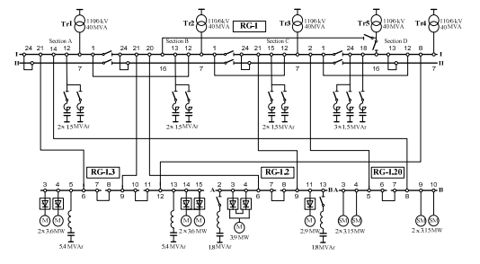
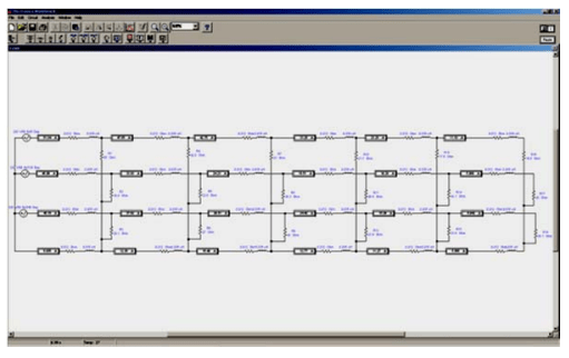
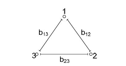
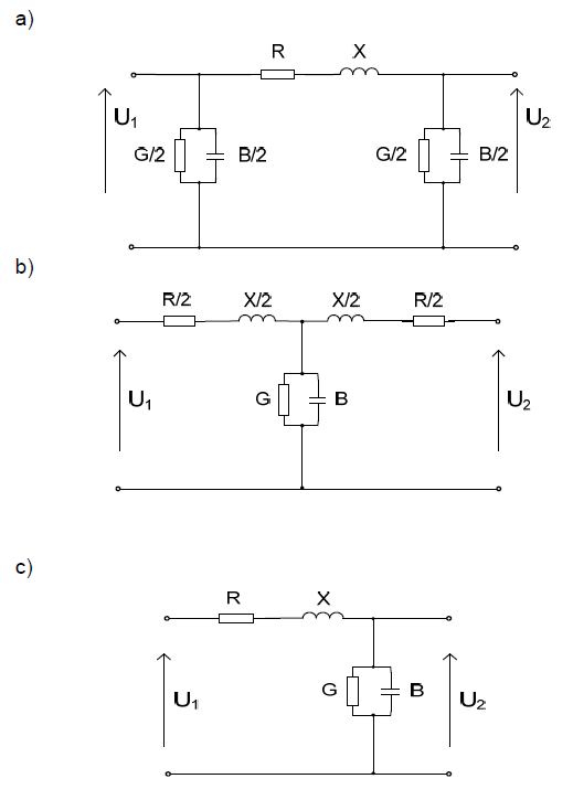
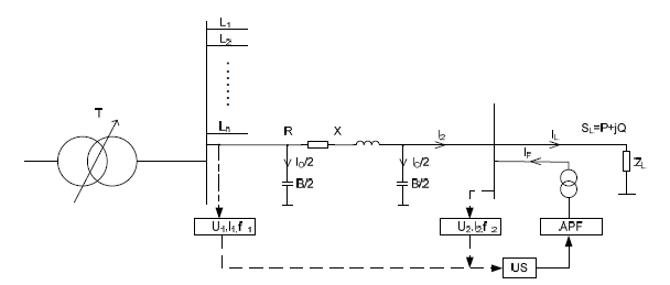
For the analysis was selected an unilaterally powered 110 kV network with a triangular arrangement of conductors (as in Fig.1). The electrical phenomena in any network are influenced, of course, by distributed line electrical parameters of both longitudinal (resistance, reactance) and transverse (conductance, susceptance). However, the analysis is usually carried out for simplicity based on one of selected equivalent model of lumped elements network type Π, T or Γ (Fig. 2) [8].

Electric models defined in per unit parameters are specified by the following relationships;

• resistance per unit R`:

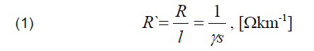
where: l -length of the network [m], γ – conductivity [m^-1Ω- 1mm^-2], s – cross-section of the conductor [mm2];

• reactance per unit X’:

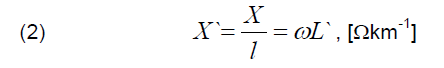
where:

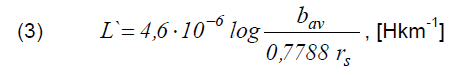
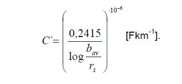
b_av – geometric mean distance between conductors [cm}

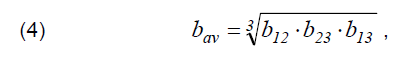
r_s– average radius (equivalent) of the conductor [cm],

• conductance per unit G’:

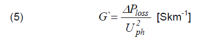
where: ΔP_loss– corona losses [kW/km], U_ph – phase voltage [kV],

• susceptance per unit B’:

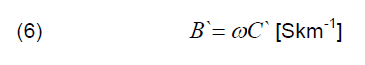
where:

Because of the problem in determination of the accurate value of active power losses due to corona effect (related significantly to the weather conditions-with the deterioration in the weather they can increase approximately by about 4- times) in the further discussion this parameter is omitted. Whereas, the value related to the current line susceptance depends on the conductor cross-section and its average value according to [3] is respectively: 120 mm²-0.169 Akm^-1, 185 mm²-0.176 Akm^-1, 240 mm²-0.203 Akm^-1, 525mm²– 0.211 Akm^-1.

For analysis the Π type model has been selected. Note, however, that accuracy of the calculations depends on the type of equivalent line model taken under consideration [2,8].

Analysis of the voltage value variation in the distribution line of 110 kV supplied unilaterally

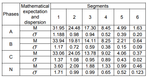
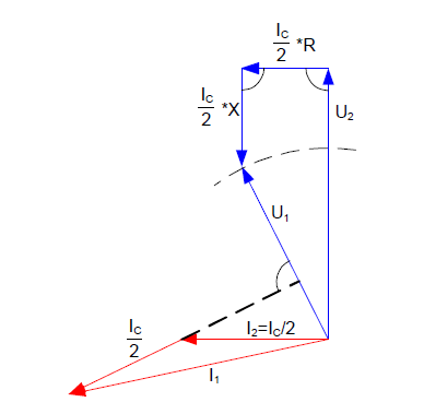
The voltage value and variation of its level at the end of the line powered unilaterally depend, of course, on the operation conditions (load). Therefore, the analysis considered both the work under loading and during the extreme case of a no-load state. Currents distribution under the no-load state is shown in Fig. 3, whereas, its vector diagram in Fig. 4 respectively.

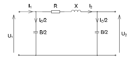
Fig.3. Equivalent scheme of the line for the no-load state considerations

Fig.4. Vector diagram of voltages and currents for the line under no-load state

Similarly the current distribution and vector diagram for the line under load is illustrated in Fig.5. and Fig. 6.

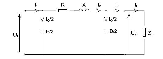
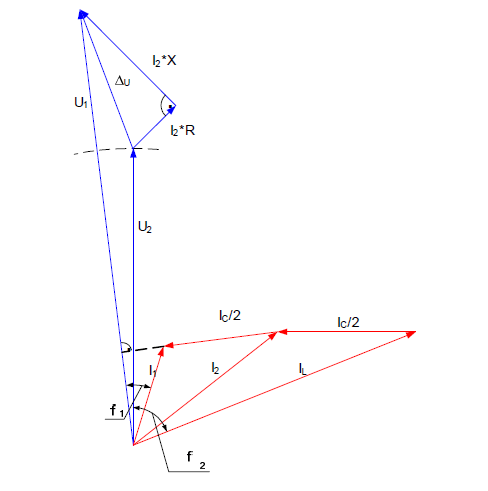
Fig.5. Equivalent scheme of the line under load

Fig.6. Vector diagram of voltages and currents for the line under load state

It should be noted that the capacitive currents I_c (I_c/2) posses constant values for the given line parameters whereas, the load current that depends on the nature (type) and the load value strongly influence the position of vectors of the voltage loss and voltage drop (vector shift) on the vector diagram. For the no-load state of the line the capacitive currents that flow in the network (so-called line charging currents) result in a voltage increase at the end of this line. On the contrary for loaded line, (with the most common load of the R, L type), there is seen an opposite effect, i.e. – the voltage value at the end of the line is decreased respectively (value of the voltage drop is dependent on the load and its character). Therefore, one can meet the following cases:

• the line capacitive current is greater than the inductive component of the load current; as a result I₁ current is capacitive,

• the line capacitive current is equal to the inductive component of the load current (line is fully compensated); current I₁ is of resistive nature,

• the line capacitive current is less than the inductive component of the load current; current I₁ is therefore inductive. Hitherto conventional methods for stabilizing the voltage level at the end of the line are based on:

• on-line regulation of the transformation ratio of the power transformer supplying the line,

• compensation of the reactive component of the line current, by

– connection of sectionalized capacitor banks at the end of the line for the case of R, L line load type,

– connection of sectionalized reactors at the end of the line for the line load current of R,C nature.

These methods have significant drawbacks and disadvantages associated with inevitability of regulation of the transformation ratio under load and/or with changeovering the sectionalized reactors (capacitors) depending on the state and nature of network load conditions (extra, expensive high voltage switches are also needed). Additional problem in modern networks to overcome is the increased level of distorted current and voltage waveforms what is the effect of application of the so called “troublous” power loads (like electric arc furnaces) and/or non-linear (e.g. power converters).

Recommended way for the voltage stabilization

Nowadays, it is possible to stabilize the voltage level by means of the active power filter (APF) connected to the end of the line (on the market there is a large gamma of ever cheaper filters with different parameters both for low and medium voltage application). However, to be effective, for analysed application, the filter has to be controlled by an algorithm developed basing on the theory of the physical components of the current (CPC) [9-11]. It may, therefore depending on the adopted function, compensate for the reactive component of the load line current (inductive and/or capacitive), resulting in variation of the voltage drop due to longitudinal parameters of the line. This filter can also produce additional capacitive load current (state of overcompensation) enabling the voltage increase over the voltage loss respectively. It can also effectively suppress higher harmonics due to non-linear loads [4,9]. This proposal is illustrated in Fig. 7.

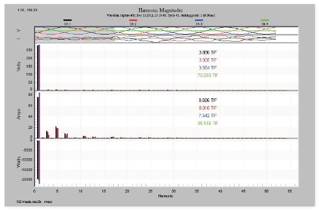
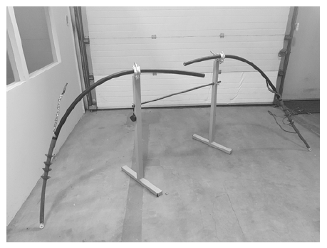
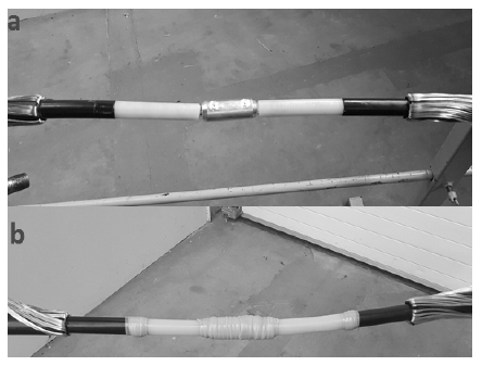
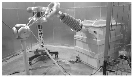
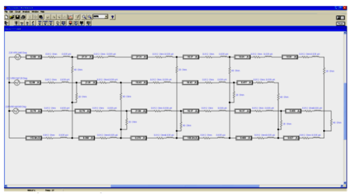
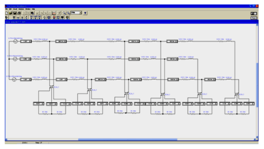
Fig.7. The way of the voltage stabilization at the end of the HV line by means of an active power filter (T-power transformer, *Z_L* –line load, R,X,B– equivalent electric parameters of the line, US-control system of active power filter, APF- active power filter)

In order to confirm the applicability of the AFP for the stabilization of the voltage in the HV line the related study were carried out for the low voltage (500 V) physical line model which simplified electric scheme is presented in Fig.8a and Fig.9a respectively. Ability to generate, by the APF arrangement, currents of a different value, nature as well as waveforms was tested carefully under various line working conditions like inductive, capacitive (no-load state of the line ) and/or inductive non-linear loads respectively. Studies have proved the usefulness of the APF for this purpose, what can be seen also from selected examples of measured and recorded waveforms shown in Fig.8 and Fig.9. In either case the active filter effectively produces the corresponding current component (inductive and/or capacitive) whereas, maintaining the line voltage at an appropriate level. The current waveforms, seen in Fig.8c and Fig.9c were generated and measured – at point 2- for a three-phase physical model of the developed filter (APF) [12-15].

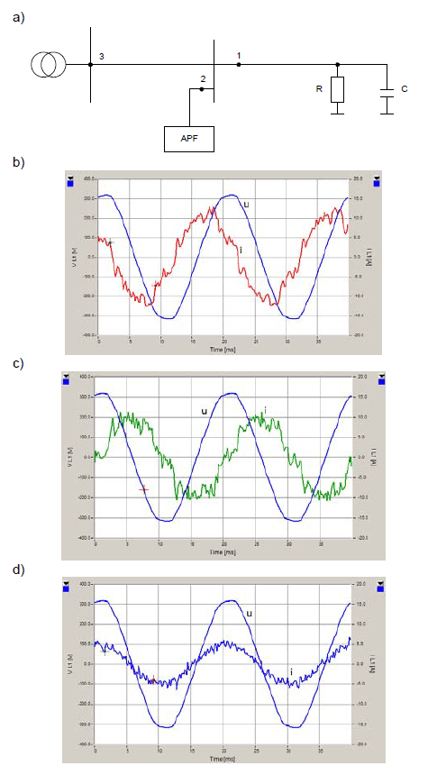
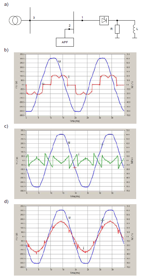
Fig.8. Schematic of the lab electric circuit (a); voltage and current waveforms (in phase L1) at the end of the line under no-load state, (b)-(measuring point-1); voltage and current of the APF (c) (measuring point 2); and resultant at the power source (d) (measuring point 3)

Fig.9. Schematic of the lab electric circuit (a); voltage- and current waveforms (in phase L₁) at the end of line when loaded with a nonlinear inductive (R,L) load (b) (measuring point 1); voltage and current t of the APF (c) (measuring point 2); and resultant at the power source (d) (measuring point 3).

If the control algorithm of the AFP introduces an additional function that allows compensation of inductive and/or capacitive current component one obtains additional effect of the power factor improvement (defined by cosφ or tanφ) at the point of connection of the line to the supply source (see Fig.8d and Fig.9d). This positively affects the whole connected electric power system.

Conclusions

The use of the active power filter (APF) is an alternative, effective way to provide voltage stabilization at the end of unilaterally fed distribution line of a high voltage. This enables compensation of capacitive currents of the line under no-load state of operation and decreases as a result the voltage value (at the end of the line) to the rated level. Under inductive R, L type of load the compensation is also performed (including power-factor correction) however, increasing the voltage at the end of the line to the rated value. As a result, it eliminates the need for expensive circuit switches to changeover the sectionalized reactors or capacitor banks. Moreover, the voltage value is on-line controlled. An additional effect that results from the use of AFP for the voltage stabilization (in HV lines supplied unilaterally) is the effective limitation (elimination) of the current harmonics level in the line currents.

REFERENCES

[1] Power conductors for overhead lines of 110kV. Technical specification of Energa-Operator, 2013.
[2] Miller P., Wancerz M., Wpływ sposobu wyznaczania parametrów linii 110 kV na dokładność obliczeń sieciowych. Przeglad Elektrotechniczny, no 4 (2014), 189-192.
[3] National Electric Power System. PSE-SF.KSEI/2005 v1. http://www.pse.pl/uplouds
[4] Wosik J., Kalus M., Kozlowski A., Miedzinski B., Habrych M., The efficiency of reactive power compensation of high power nonlinear loads, Elektronika ir Elektrotechnika, vol. 19, no. 7, (2013), 29–32.
[5] Hou R., Liu J. W. Y., Xu D., Generalized design of shunt active power filter with output LCL filter, Elektronika ir Elektrotechnika, vol. 20, no. 5 (2014), 65–71.
[6] Woodley, N. H., Morgan, L., Sundaram, A. Experience with an inverter-based dynamic voltage restorer. IEEE Transactions on Power Delivery, 14(3) (1999), 1181-1186.
[7] Nielsen, J. G., Newman, M., Nielsen, H., Blaabjerg, F. Control and testing of a dynamic voltage restorer (DVR) at medium voltage level. IEEE Transactions on power electronics, 19(3) (2004). 806-813.
[8] Konczykowski S., Electrical Power Networks. WNT, Warszawa, 1971 (in polish).
[9] Habrych M., Wisniewski G., Miedzinski B., Wosik J., Kozlowski A., Possibility of load balancing in Middle Voltage network with the use of Active Power Filter, Elektronika ir Elektrotechnika, no.5 (2015), 19-23.
[10] Czarnecki, L. S. Orthogonal decomposition of the currents in a 3-phase nonlinear asymmetrical circuit with a nonsinusoidal voltage source. IEEE Transactions on Instrumentation and Measurement, 37(1), (1988), 30-34..
[11] Czarnecki L. S., Powers of asymetrical loads in therms of the CPC theory, Electrical Power Quality and Utilisation Journal, vol. 13, no 1 (2007), 97–103.
[12] Kamal R., Sharma K., Voltage regulation using FACTS devices. International Journal of Pure and Applied Mathematics, Vol. 119, no 16 (2018) 2207-2214.
[13] Pais M., Almedia M.E., Castro R., Voltage regulation in low voltage distribution networks with embedded photovoltaic microgeneration. International Conference on Renewable Energies and Power Quality (ICREPQ12), Santiago de Compostela, (2012).
[14] Zou Z. X., Zhou K., Wang Z., et al., Frequency-adaptive fractional order repetitive control of shunt active power filters, IEEE Trans. on Industrial Electronics, vol. 62, no. 3 (2015), 1659–1668.
[15] Kotsalos K., Decentralized voltage regulation in radial
medium voltage networks with high presence of distributed generation, Journal of Engineering, 3, (2017), 26-38.

Authors: dr inż. Julian Wosik, Instytut Technik Innowacyjnych EMAG, ul. Leopolda 31, 40-189 Katowice, dr hab. inż. Marcin Habrych, prof. uczelni, Politechnika Wrocławska, Katedra Energoelektryki, Wybrzeże Wyspiańskiego 27, 50-370 Wrocław, Email: marcin.habrych@pwr.edu.pl, prof. dr hab. inż. Bogdan Miedziński, Politechnika Wrocławska, Katedra Energoelektryki, Wybrzeże Wyspiańskiego 27, 50-370 Wrocław, E-mail: bogdan.miedzinski@pwr.edu.pl, dr inż. Grzegorz Debita, Akademia Wojsk Lądowych imienia generała Tadeusza Kościuszki, ul. Czajkowskiego 109, 51 – 147 Wrocław E-mail: grzegorz.debita@awl.edu.pl, dr inż. Andrzej Firlit, Akademia Górniczo-Hutnicza im. Stanisława Staszica w Krakowie, Katedra Energoelektroniki i Automatyki Systemów Przetwarzania Energii, al. Mickiewicza 30, 30-059 Kraków, E-mail: andrzej.firlit@keiaspe.agh.edu.pl

Source & Publisher Item Identifier: PRZEGLĄD ELEKTROTECHNICZNY, ISSN 0033-2097, R. 96 NR 1/2020. doi:10.15199/48.2020.01.29

Understanding Telephone Interference Factor

Published by David Horning, March 2013. Power Monitors, Inc., White Paper: Understanding Telephone Interference Factor

Abstract. Harmonic distortion that is produced from power conversion systems can cause interference on analog telephone lines. The degree of telephone interference can be expressed in terms of the Telephone Interference Factor (TIF). This white paper will discuss how interference is generated, how TIF is calculated and how PMI’s power quality recorders can provide the user with these measurements.

Telephone Interference

As mentioned above, the TIF is a measure of the potential telephone noise caused by the harmonic distortions from a power system on nearby telephone equipment. It is a dimensionless quantity that depends upon a weighting factor derived from 1960 weighting curve by the Edison Electric Institute (See Figure 1). This weighting factor is weighted heavier on frequencies that tend to cause interference in the audible range and are based on the response of the human ear. The higher the factor the more interference is being generated. Other forms of communication, besides telephones, are also effected.

The TIF weighting factor was originally developed by placing power lines close to un-shielded telephone lines. A group of people were asked to compare the noise, in a telephone receiver, to a buzzing noise and adjust the buzzer so that it was equally disturbing as the noise to be measured. Later this factor was revised and extended to higher frequencies.

Interference on communication lines happen for several reasons. Power stations transmit very high energy and telecom systems transmit much smaller signals. Power and telecom cables are often close together and run in parallel for long distances. Power transmissions produce electric and magnetic fields which can induce noise on the telecom systems communication lines. Several powerline communications systems can cause telephone interference. High current systems like TWACS can inductively couple to telephone lines, but by their nature are more transitory. Slow, narrowband systems like TS2 signals are usually too low to be problem, however, improper grounding at the substation can cause the transmitter voltage signal to be coupled into the telephone system.

Harmonic voltages and currents, especially high frequency harmonics generated by in rotating machinery and adjustable speed drives, can have a serious impact on telecom systems. Distortion in harmonics between 540 Hz (9th harmonic) and 1200 Hz (20th harmonic) are particularly disruptive.

Most of the distortion is produced by the load but power generation can also produce distortion. Voltage TIF can be an issue resulting from the output of a generator or UPS. Some generators have a TIF specification, but often do not. Inverters fed from solar panels, windmills, etc. Synthesize a sine wave, and often have harmonic content that can create audio problems through telephone line coupling as well as direct interference through AC powered audio devices.

Telephone interference is often expressed as a product of current and TIF. Since traditional telephone interference was inductively coupled, the current harmonics are usually examined with TIF. Voltage harmonics can also be a problem though, most often due to grounding differences between the telephone and power networks.

Telephone interference was a severe problem in the days of open wire telephone circuits. Now with shielding and twisted pair conductors it is not as much of a problem. Telecom systems design takes into consideration interference and noise and the are mitigating systems that can reduce the effect of the interference. Reducing interference is a joint effort with the power producers, telecom company, power consumers, and equipment producers.

Calculation

Formula:

Where:

X = Total RMS voltage or current
X_n = Single frequency RMS current or voltage at the frequency corresponding to harmonic order n
W_n= Single frequency TIF weighting at the frequency corresponding to harmonic order n

Provision and TIF

TIF is computed by ProVision from the harmonics of captured waveforms. In ProVision, after loading a waveform capture, it’s possible to click on the harmonic toolbar icon to switch to a harmonic analysis of that waveform. It is also possible to go directly to that with Graph, Harmonic Analysis, Magnitudes on the toolbar. Once there (after selecting a waveform capture record), THD will be visible, drawn on the graph.

A little known fact is that those graph annotations are clickable. After clicking a few times, it will switch to showing TIF for the displayed waveforms as shown in Figure 2. To select the cycle that is being computed, move the grey cycle in the top trace to select the appropriate cycle.

Figure 2. Clicking THD graph annotations in ProVision shows TIF

It’s important to carefully select the cycle that is analyzed. Move the grey box at the top of the graph around to pick a cycle of data form in the waveform capture to select a “typical” looking cycle,. Often, waveform capture is triggered based on an event like a voltage sag, etc., and the waveform capture includes non-normal cycles. TIF, like harmonics, are a steady-state phenomenon, so it is necessary to select a waveform that is representative of the steady-state wave shape, not one during a PQ event. The very first, and sometimes very last cycles in the capture are often the most representative, due to the pre- and post-cycle parameters with waveform capture.

Alternatively, periodic waveform capture can be enabled, and this allows the capture of “normal” waveforms. To learn more about waveform capture refer to the whitepaper Harmonics from Periodic Waveform Capture available HERE.

Conclusion

• Harmonic distortion can have a large effect on communication systems. This effect is known as Telephone Interference Factor (TIF). The factor has been revised during the year as technology changes.

• Interference is often expressed as a product of current and TIF. Other forms of communication, besides telephones, are also effected.

• Reducing interference is a joint effort with the power producers, telecom company, power consumers, and equipment producers.

• Using TIF as a measurement for working with telephone noise is a simple process, especially when using ProVision and one of PMI’s many harmonics enabled recorders

Author: David Horning, Software Developer, Email: dhorning@powermonitors.com, Website: http://www.powermonitors.com, Phone no. (800) 296-4120

Multi-Servers System with Firebird Database for Automatic Reactive Power Compensation

Published by Marian HYLA, Silesian University of Technology, Department of Power Electronics, Electrical Drives and Robotics

Abstract. The paper presents the concept, implementation and operational effects of the multi-servers automatic reactive power compensation system in 6 kV industry electrical power grid. As controlled reactive power compensators were used synchronous motors, capacitors’ banks and passive filters of higher harmonics available in the power grid of the plant. System of communication and collaboration of control servers with databases was disclosed. Use of events technology of Firebird database was discussed. Clients’ application for industry grid state and compensation system monitoring were presented. Results of operation and planned modernization of the system was presented.

Streszczenie. W artykule przedstawiono koncepcję, realizację praktyczną oraz efekty działania wieloserwerowego systemu automatycznej kompensacji mocy biernej w przemysłowej sieci elektroenergetycznej 6 kV. Jako kompensatory mocy biernej wykorzystane zostały silniki synchroniczne, baterie kondensatorów i pasywne filtry wyższych harmonicznych pracujące w zakładzie. Przedstawiono system informatyczny i współpracę z bazą danych. Omówiono wykorzystanie technologii zdarzeń bazy danych Firebird w prezentowany rozwiązaniu. Przedstawiono oprogramowanie klienckie wykorzystywane do monitorowania pracy systemu i stanu sieci elektroenergetycznej. Przedstawiono przykładowe efekty działania oraz propozycje dalszych prac związanych z modernizacją systemu. (Wieloserwerowy system automatycznej kompensacji mocy biernej z bazą danych Firebird)

Keywords: reactive power compensation, power factor correction, automatic control, data bases, Firebird events technology, monitoring
Słowa kluczowe: kompensacja mocy biernej, współczynnik mocy, automatyczna regulacja, baza danych, technologia zdarzeń bazy Firebird, monitorowanie

Introduction

Reactive power compensation is aimed to relieve an electrical grid of reactive currents flow, what is achieved by elimination the phase shift between the fundamental voltage and current harmonics and by elimination of higher harmonics in the load current regardless of the form of the supply voltage [1, 2]. In such conditions minimizing current and apparent power of the source for a given active power of the load is achieved. In practice, there are many definitions of reactive power [3, 4, 5]. In many industrial electrical grids, is applied a partial compensation, based on the fundamental voltage and current harmonics compensation to maintain a power factor value within the desired range. For this purpose, as a source of reactive power are used capacitors, harmonics passive filters and synchronous compensators both in the form of unloaded and underloaded synchronous motors or generators [4, 6, 7, 8, 9, 10]. Passive harmonic filters used for eliminating selected harmonics are also sources of reactive power of the fundamental harmonic and can be used for tgφ factor correction.

Failure to comply with the relevant technical parameters of the power consumed by customers at points of connection to the supplying power grid causes in additional fees charged by electricity suppliers. To reduce the costs of electricity reactive power consumed from the supply grid at each of the supply points of the plant should be compensated.

The technical benefits effecting from the reactive power compensation are [1, 6, 11, 12, 13, 14, 15]:

• increasing the possibility of active power flows at the same nominal current of power lines or the same active power flows at reduced line current,

• improving voltage conditions of the grid by reducing the voltage drops,

• reducing energy losses caused by reactive current flows,

• reducing equipment failures by limiting the voltage variations in the grid,

• improving power supply reservation conditions and reliability.

The economic benefits of reactive power compensation are [11, 16]:

• reducing fees for active energy consumed to cover transmission of reactive power losses,

• eliminating extra fees charged for non-optimal reactive power consumption: consumption of electric energy with tgφ factor higher than specified in the contract, consumption of inductive reactive energy without active energy consumption and consumption of active energy with capacitive power factor.

At varying active and reactive power consumption caused by a plant production cycle, the solution is automatic, real-time, follow-up reactive power compensation system, allowing independent compensation of each supply point. For this purpose reactive power sources available in the internal power grid are used.

Concept of the automatic reactive power compensation system

Concept of the automatic reactive power compensation system is shown in Figure 1. The task of the compensation system are active and reactive power measuring in supply points of the plant, identification of the actual grid configuration and proper reactive power distribution to the individual, currently available, adjustable sources of reactive power. This task is performed by the main controller.

Synchronous machines local controllers are designed to supply given reactive power ensuring proper operation of the drive in the synchronous state [17]. Synchronous operation state is required by superior function of the drive system. Described implementation uses the ProgressPOWER microprocessor-controlled power supply units for the excitation of synchronous motor [18]. This device was developed in co-operation with the author.

Local controllers for switching capacitor banks and filters of harmonics are parts of communication system. Control of capacitor banks matched with control of synchronous compensators realized properly by the main controller holds the power factor in the desired range [19]. Long term variations of reactive power caused by a plant production cycle are compensated by switching the appropriate sections of capacitors. Underloaded synchronous machines in the system of compensation allow step less (continuous) reactive power regulation. They are used for reactive power momentary fluctuations compensation [2, 10, 18, 19, 20].

The adjustable value is power factor tgφ expressed by the equation:

where: P – active power, Q – reactive power. The control algorithm based on measurements at the supply point of the plant determines the actual demand for change of reactive power of the supply transformer according to the equation:

where: ΔQ_z– required change of reactive power in the actual step of the regulation process, P, Q – the actual active and reactive power at the supply point, tgφ_z – required power factor at the power supply point of the plant.

Reactive power which should be generated by n available compensators is expressed by the relation:

where: Q_i – actual reactive power of i-compensator.

The problem of the reactive power optimization with additional criteria and restrictions in multilevel industry grid based on presented solution is analysed in [22]. Calculation algorithm aim to fulfill equation (3) ensuring power factor at the supply point of the plant at the required range.

To enable the independent automatic compensation of each supply point the actual grid configuration should be known by the main controller. Figure 2 shows a part of the grid identified by one of the main controllers of described implementation.

Fig.2. Part of the grid identified by the main controller of automatic reactive power compensation system

Identified are states of switches and disconnectors in each of the fields of the switching stations shown in Figure 2. This allows to match supplying transformers with each compensator. There are measured electrical parameters in each of the 110/6 kV power supply transformer and thyristor hoisting machines current. Measurement of hoisting machines current is to determine whether the machine operates, what requires switching on the appropriate filters of harmonics. There are also available measurements of synchronous drives, transmitted to the main controller by the local controllers of the synchronous machines. The state of the grid and measurements are stored in the database, enabling later system operation analysis.

Informatics structure

The presented idea of the automatic reactive power compensation system has been implemented in a large mining plant in Poland. A characteristic features of the plant grid are a considerable distance between the supply switching stations of the plant up to several km and the fact that separate parts of the grid are supplied independently.

In Poland energy costs for industrial plants are calculated separately for each power supply point. For this reason it was decided to use multi-servers system which allows autonomous operation at each location, and at the same time it is prepared to work in the event of payment calculation change e.g. fees calculation based on groups of power suppling points or even for the entire plant.

Figure 3 shows the informatics structure of the realized multi-servers reactive power compensation system. Control servers perform functions of main controllers as shown in Figure 2. Each control server is responsible for the independent part of the grid and cooperates with its own database.

The described system consists of:

• 4 control servers and 4 databases,
• 9 switching stations 6 kV,
• 12 power supply transformers 110/6 kV,
• 22 sections of capacitors’ banks of power ratings from 0.6 up to 2.4 MVAr,
• 4 filters of harmonics of power ratings from 1.8 up to 5.4 MVAr

• 10 synchronous motors drive of fans with a power ratings from 1.5 up to 3.15 MW equipped with a microprocessor controlled unit for excitation with reactive power regulator [18],

• switches position identification for about 100 selected fields of selected internal switching stations.

Fig.3. Informatics structure of multi-servers reactive power compensation system

Communication in the system is carried out by Ethernet but some of devices are communicating with the control servers via RS-485 interface witch MODBUS protocol. Control servers provide information about the realized compensation process to clients’ applications. The client application has the ability to monitor the status of a part of the grid managed by each server and has got access to each database.

Events technology of Firebird database

Information about system changes is transmitted by the events technology of Firebird database [23, 24]. Events are simple notification messages transmitted asynchronously from the database server to the clients’ applications, initialized by the server. They act in a different way comparing to the typical mechanism of request-reply SQL databases.

Fig.4. Diagram of client software and Firebird database server connecting process with support for events technology

The mechanism of events uses an additional connection between the Firebird database server and a client’s application. After the client establishes a connection to a standard port to query SQL (RemoteServicePort), the server offers an additional communication channel by opening an additional port defined by the RemoteAuxPort configuration parameter and sends to the client information about this port number. The client’s application interested in receiving events may establish the additional connection to the offered RemoteAuxPort port. Diagram of client software and database server connecting process, with support for events technology, is shown in Figure 4 [25].

After establishing a connection with RemoteAuxPort the clients’ application declares that events are in the range of its interest by registering names of events in the Firebird database server.

After the event appears all clients’ applications that have registered this event will be informed of its occurrence. Clients receive information about the name of the event and the number of its appearance. Reaction of the client’s application to retrieve information about occurrence of such event depends on the programmer.

The event may be generated by the server for various cases set by the database administrator. As example in the described implementation, events associated with the grid configuration changes are generated by data table trigger. Trigger forwards the name of the table to the stored procedure. Next, the stored procedure calls POST_EVENT procedure with the received parameter. In this example, structure of a table containing information about the grid configuration and changes can be created by the command shown in Figure 5.

The INPUT field contains the number of the changed signal. The INPUTS_1 … INPUTS_N fields contain the binary values of all signals states.

In order to provide information about the table where change occurred it was created the stored procedure with one input parameter. The parameter content is passed by trigger which executed this procedure.

Fig.5. Database table creation algorithm

Fig.6. Stored procedure creation algorithm

Fig.7. Database table trigger creation algorithm

Fig.8. Refreshment of actual grid configuration SQL-query

Fig.9. Monitoring of the reactive power compensation system and the grid state: a) measurements in power supply points of the plant, b) electrical grid configuration

To automate the events transfer process triggers in the selected tables are created. For example, trigger for GRID_CONFIG table is created by the command shown in Figure 7. Thanks to use the Firebird database events technology, there is no need of periodical data refreshment to detect changes in the content stored in the database. Information is downloaded only in case of real change of the database content.

Detection of the regulation procedure parameters changes is realized in a similar way. Authorized user of client’s application can set: given value of the power factor, switching time limits of capacitors’ banks and filters of higher harmonics, values of currents and time intervals to determine stops of hoisting machines, etc.

Monitoring of the system

Information from control servers and databases of the reactive power compensation system allowed to design clients’ software for monitoring the compensation processes and for the electrical grid state visualization.

Communication is established by direct TCP/IP connections to each control server, combined with connection to each Firebird database with events receiving possibility.

The software is intended for use in PCs with Windows operating system and can run in desktop mode or in the touch panel mode, e.g. embedded in the control cabinet.

Clients’ applications provide access to actual and historical information related to the power grid state and to each compensator used in the reactive power compensation system. Examples of the information available in clients’ software in the touch panel mode are shown in Figure 9.

Fig.10. Active (P) and reactive (Q) power measured waveforms of thyristor’s hoisting machine during the operation cycle

Results of operation

Figure 10 shows the active and reactive power measured waveforms of thyristor’s hoisting machine during the operation cycle.

It can be observed sudden changes of active power of few MW and reactive power of several MVAr. The highest consumption of reactive power occurs when thyristors are working with angle around 90^o, so when the hoisting engine is starting. Such reactive power changes are not possible to compensate by capacitors’ banks. Switching of capacitors’ banks is limited by need of their discharging before next switching on. However it is possible to compensate such a reactive power changes by follow-up compensation using controlled synchronous machines.

Fig.11. Measurement waveforms of active and reactive power in one of the plant supply points and corresponding average 15 min. tgφ factor

Figure 11 shows the selected measured waveforms in one of the power supply transformers of the part of the grid presented in Figure 3 and corresponding averaged 15- minute tgφ measurements with the automatic reactive power compensation system implemented in the mining plant. As controlled sources of reactive power were used capacitors’ banks and synchronous motor drives of the mine main ventilation system fans. Harmonics’ filters of working hoisting machines have been switched on permanently. The required value of tgφ factor was 0.2 and acceptable values should stay in the range of 0.0-0.4.

Selected waveforms include the periods of operation and stoppage of hoisting machines. In the present case effectiveness of compensation for load variations shown in Figure 11 depends on the regulation range of adjustable follow-up reactive power synchronous machines. These are underloaded high power synchronous motors driving the mine underground ventilation fans. These synchronous motors are equipped with microprocessor controlled units for excitation supply.

Conclusions and future work

Many enterprises cover the additional costs of electrical energy caused by improper management of the reactive power in spite of sufficient quantity of compensators and possibilities of controlling them. Experience taken from many Polish plants shows that attempts of reactive power compensation realized by human operators are often insufficient to provide the desired power factor. These attempts don’t allow to take into account other optimization criteria.

The solution is the real-time follow-up automatic reactive power compensation system responsing to: active and reactive power load changes, switching in the plant power grid, compensators availability and control range changes. Practical experience shows that the presented reactive power compensation system allows to utilize full compensation abilities of installed devices. It makes possible to eliminate or substantially reduce the additional fees for exceeding reactive power out of allowable range. Presented, developed by the author, multi-servers automatic reactive power compensation system has been implemented by JJA Progress company in the large mining plant in Poland.

Actually some elements of the system, due to its design, use a RS-485 communication standard. Planned modernization is based on use of hardware RS-485 to TCP/IP converters, allowing all devices to be accessed via Ethernet. Thanks to that each control server will get ability to communicate with each component of the system. This will increase the system reliability by replaceability of tasks performed by each server. Failed server will be automatically replaced with another.

Despite of developing new compensation equipment such as: static Var compensators (SVCs) with thyristor-switched capacitors (TSCs), thyristor-controlled reactors (TCRs), self-commutated pulse width modulation (PWM) converters capable properly control generation or absorption of the reactive power, the reactive power compensation in industrial power grids realized by capacitors’ banks, passive harmonics filters and underloaded synchronous machines is often acceptable for the users, both in technical and economic terms.

REFERENCES

[1] Dixon J., Moran L., Rodriguez J., Domke R.: Reactive Power Compensation Technologies: State-of-Art Review, Proc. of the IEEE. Vol.93. No.12, 2005, pp.2144-2164
[2] Igbinovia F. O., Fandi G., Švec J., Müller Z., Tlusty J.: Comparative review of reactive power compensation technologies, 16th International Scientific Conference on Electric Power Engineering (EPE) 2015, Kouty nad Desnou, 2015, pp.2-7
[3] Fryze S.: Active, reactive and apparent powers in nonsinusoidal systems (in Polish), Przegląd Elektrotechniczny, no. 7/1931, pp.193-203
[4] Ortega J. M. M., Payan M. B., Mitchell C. I.: Power factor correction and harmonic mitigation in industry, Industry Applications Conference, 2000. Conference Record of the 2000 IEEE, Rome, 2000, vol.5, pp.3127-3134
[5] Balci M. E., Hocaoglu M. H.: Comparison of power definitions for reactive power compensation in nonsinusoidal conditions, 11th International Conference on Harmonics and Quality of Power, 2004, pp.519-524
[6] Angelo B.: Handbook of Power Quality. John Wiley & Sons, 2008
[7] Fehr R.: Power Factor Correction. In Industrial Power Distribution , Wiley-IEEE Press, 2016, pp.319-330
[8] Heger C. A., Sen P. K., Morroni A.: Power factor correction — A fresh look into today’s electrical systems. 2012 IEEEIAS/PCA 54th Cement Industry Technical Conference, San Antonio, TX, 2012, pp.1-13
[9] Xu H., Wang C.: Power Factor Improvement in Industrial Facilities Using Fuzzy Logic Excitation Control of Synchronous Motor, International Conference on Computational Intelligence and Software Engineering, CiSE 2009, Wuhan, 2009, pp.1-4
[10] Al-Hamrani M. M., Von Jouanne A., Wallace A.; Power factor correction in industrial facilities using adaptive excitation control of synchronous machines, Conference Record of the 2002 Annual Pulp and Paper Industry Technical Conference, Toronto, Ontario, Canada, 2002, pp.148-154
[11] Yehia M., Ramadan R., El-Tawil Z., Tarhini K.: An Integrated Technico-Economical Methodology for Solving Reactive Power Compenation Problem, IEEE Transactions on Power Systems, Vol. 13, No. 1, 1998, pp.54-59
[12] Ekel P., Ansuj S., Schinzinger R., Prakhovnik A., Razumovsky O.: Automation of reactive power compensation in industrial power systems, Proc. of the Third IEEE Conference on Control Applications, Glasgow, 1994, vol.1, pp.479-484
[13] Herman L., Papic I.: Optimal control of reactive power compensators in industrial networks, Proc. of 14th International Conference on Harmonics and Quality of Power – ICHQP 2010, Bergamo, 2010,pp.1-6
[14] Das J. C.: Reactive power flow control and compensation in the industrial distribution systems, Industrial and Commercial Power Systems Technical Conference, Conference Record, Papers Presented at the 1993 Annual Meeting, St. Petersburg, FL, USA, 1993, pp.128-136.
[15] Helmi B. A., D’Souza M., Bolz B. A.: The application of power factor correction capacitors to reserve spare capacity of existing main transformers, Industry Applications Society 60th Annual Petroleum and Chemical Industry Conference, Chicago, IL, 2013, pp.1-6
[16] Li F., Zhang W., Tolbert L. M., Kueck J. D., Rizy D. T.: Assessment of the Economic Benefits from Reactive Power Compensation, 2006 IEEE PES Power Systems Conference and Exposition, Atlanta, GA, 2006, pp.1767-1773
[17] Schaefer R. C.: Excitation control of the synchronous motor, IEEE Tran. Ind. Appl. 1999, 35(3), pp.694–702
[18] Hyla M.: Power supply unit for the excitation of a synchronous motor with a reactive power regulator, Mining – Informatics, Automation and Electrical Engineering, 1(521), 2015, pp.17-21
[19] Sagiroglu S., Colak I., Bayindir R,: Power factor correction technique based on artificial neural networks, Energy Conversion and Management, vol .47, no. 18-19, November 2006, pp.3204-3215
[20] Colak I., Bayindir R., Bay O.F.: Reactive power compensation using a fuzzy logic controlled synchronous motor, Energy Conversion and Management, vol. 44, no. 13, August 2003, pp.2189-2204
[21] Wysocki W., Szlosek M.: Compensation of reactive power as a method for reducing energy losses: On the example of calculations and measurements of load flow through the distribution transformer in one of the polish distribution network, 2011 11th International Conference on Electrical Power Quality and Utilisation (EPQU), Lisbon, 2011, pp.1-5
[22] Hyla M., Gierlotka.K.: The optimization on the control of reactive power compensators in industry power grid, International Conference on Electrical Drives and Power Electronics. EDPE 2003, The High Tatras, Slovak Republik, 24-26 September 2003, pp.422-427
[23] Borrie H.: The Firebird Book. A Reference for Database Developers, Apress, 2004
[24] Babuskov M.: The Power of Firebird Events, Firebird Conference, 13-15.12.2005, Prague 2005

Autor: dr inż. Marian Hyla, Silesian University of Technology, Faculty of Electrical Engineering, Department of Power Electronics, Electrical Drives and Robotics, ul. B. Krzywoustego 2, 44-100 Gliwice, Poland E-mail: marian.hyla@polsl.pl

Source & Publisher Item Identifier: PRZEGLĄD ELEKTROTECHNICZNY, ISSN 0033-2097, R. 94 NR 8/2018. doi:10.15199/48.2018.08.27

Obtaining Feasibility of Power Flows in the Deregulated Electricity Market Environment

Published by Mariusz DRABECKI, Eugeniusz TOCZYŁOWSKI,
Warsaw University of Technology, Institute of Control and Computation Engineering

Abstract. In this paper we analyse a power dispatch method for obtaining feasible power flows, both active and reactive power, in terms of satisfying the transmission, voltage level and voltage angles’ constraints, under assumption that supply of electric power is directly contracted by the market participants in the deregulated environment, through energy trade. The method is based on solving two optimization problems originated from Optimal Power Flow standard formulations, which can be solved by system’s operator. The approach was tested on 9-bus test system, under three different loading scenarios.

Streszczenie W artykule przedstawiono metodę otrzymywania dyspozycji mocy, dającej dopuszczalny rozpływ mocy, zarówno czynnej jak i biernej, przy założeniu, że dostawa energii jest kontraktowana bezpośrednio pomiędzy uczestnikami zderegulowanego rynku. Metoda bazuje na wykorzystywaniu dwóch zadaniach optymalizacji, wyprowadzonych od standardowego zadania typu Optimal Power Flow. Prezentowane podejście zostało przetestowane symulacyjnie na 9-węzłowym systemie testowym, przy trzech różnych scenariuszach obciążenia (Otrzymywanie dopuszczalności rozpływu mocy).

Keywords: deregulated electricity market, Optimal Power Flow, network feasibility of power flow, power systems.
Słowa kluczowe: zderegulowany rynek energii, Optimal Power Flow, dopuszczalność sieciowa rozpływu mocy, systemy elektroenergetyczne

Introduction

In the last decades, we observe trends of transforming the power systems’ architectures from totally controlled by the system operators towards completely deregulated ones, see [1]. In the traditional, centralized approach, generating units are often dispatched by the systems operators who may also participate in contracting supply of electrical energy from market participants. However, this is not the case in the deregulated systems, where it is up to participants to agree on contracts between consumers and suppliers and therefore to allow suppliers to plan the unit self-commitment and self-dispatch of the generation units.

These agreements are likely to be made without considering feasibility issues of the delivery through power flow analyses. As it was shown in [2], network feasibility of power flow (power flows, nodal voltages and angles being within their technical limits), considering both active and reactive flow, depends highly on grid model used for determining the power dispatch. Thus, when units are dispatched basing only on individual participants’ preferences, as in the deregulated systems, it is possible to obtain dispatch that yields an infeasible flow. So, it is important to find a way of obtaining feasible re-dispatch which would take into account individual agreements between market participants.

According to authors of [1,3,4], the technical feasibility issues might be addressed by installing controllable hardware access terminals at generation/load bus level. These devices will need to have capabilities of limiting possible generation/demand of a given market participant to ensure network feasibility of the dispatch.

We shall consider a typical scenario in which the power system under consideration may be a local grid, or a wider area sub-network, managed by the system operator striving for system self-balancing.

Some research has already been conducted in looking for ways of dispatching generating units in distributed and deregulated environments. However, nowadays it is the system operator who knows best all technical limits of the power system. Thus, it is reasonable to assume that, at least in the period of transition from regulated to deregulated architecture, the system’s operator is a relevant entity to guard security and stability of power supply to its customers.

Authors of [4, 5, 6] approached the self-balancing problem by solving optimization problems, such as the economic dispatch or OPF/DC-OPF ones. However, these research works focused solely on minimizing the social welfare function, neglecting contracts made freely between consumers and suppliers of electric power. What is more, in these works the role of system’s operator remains unclear and possibly suppressed.

In the power system under consideration, the system operator for re-dispatching purposes may procure balancing energy from local energy sources/demands, or from a wider area network system which is connected to, and assures central control of the access terminals at the generation/load bus level. The balancing energy can be provided by suppliers, or by consumer`s loads through various demand-side response programs. For simplicity, we neglect option that the system operator procures other balancing services, such as reserves.

In this paper we analyze the approach for central balancing and control of the proposed access devices. System operator may perform the task with the help of solving some network flow optimization problems, to ensure that the resulting dispatch would yield feasible power flows in terms of all technical constraints. The first attempt is based on adjusting levels of generation only at some nodes, while in the second stage joint adjustments of loads and generation are taken into account at all nodes.

For the adjustment tasks we use the network flow formulations that are based on standard Optimal Power Flow (OPF) problem [7] extended to consider contracts signed directly between the market participants without obtaining prior approval from system’s operator.

Proposed approach

In this section the proposed balancing approach is described in detail. As it was already stated, we want to find a way of obtaining network feasible flows, resulting from dispatch, that specifically addresses contracts made directly between market participants, while by-passing operator’s governance.

We shall consider two network flow optimization subproblems formulated further in this section. The first subproblem controls solely generating units only and the second allows also load reductions at the bus level. Both proposed formulations are the restrictions of the standard OPF problem. Thus, any feasible solution of one of these two sub-problems would yield a network feasible power flow in terms of satisfying technical constraints.

In these formulations, contracts made between market participants provide resulted contract positions of the suppliers and loads, and therefore are included as soft limits within the optimization problems, both on generation and demand side.

As contracts are signed directly between market players, overall generation cost (social welfare function) is unknown and is of little interest to the operator. Thus, the cost function can be only comprised of the cost associated with soft violations of the market positions (by adjustments through selling and buying balancing energy at network nodes).

To assure that the resulted power flow is technically feasible, the operator can follow the following generic steps:

0. Accept contracts between suppliers and consumers that lay within all technical limits of generating units, i.e. which do not exceed its technical maxima/minima. Architectural design of an appropriate IT platform is beyond the scope of this article and will not be elaborated.

1. Check the network feasibility of power flow that results from accepted contracts between generators and consumers. If necessary, in case of infeasibility, re-dispatch by adjusting levels of generation only at some nodes. For this purpose we use Formulation (2) of problem described below.

2. If Step 1 does not provide feasible solutions, the reduction of the demand in some nodes may be necessary to obtain feasibility. This can be done jointly by adjustments of both loads and generation in some nodes. For this task we use Formulation (3) described below.

Optimal Power Flow Problem (OPF)

The OPF problems are well-known and widely used nonlinear and non-convex optimization problems, solved by system operators for determining feasible active and reactive power dispatch.

Usually, OPF is a problem of minimizing the total generation cost, with respect to all system constraints such as technical maxima/minima of generating unit constraints, line flow constraints, voltage levels and angle constraints and power balance constraints. However, different other cost functions can be also used, such as: minimization of transmission losses or redispatch of reactive power for enhancing the level of system’s stability such as was done in [8].

Below, in (1), we cite a simplified formulation of the OPF problem as was given in [7,9], with standard cost function i.e. minimization of the overall generation costs:

where: ݂f_P – the total cost of generation and transmission, ܰN – set of all buses in the system, ܰN_G – set of all generating units, ܰN_f – set of all branches in the system, ܲP_i^inj/ܳQ_i^inj – active / reactive power injection at bus i calculated using standard power flow equations [7], P_i^D/ܳQ_i^D– active/reactive power demand at bus i, P_i/ܳD_i – active/reactive output of unit i, Q_i^min/max / P_i^min/max– generation limits of unit i, U_i – voltage magnitude at bus i, U_i^min/max– limits on voltage magnitude of bus i, Θ_i– voltage angle at bus i, Θ_i^min/max – limits on voltage angles of bus i, S_l – apparent power flow through line l, S_l^max– maximum value of apparent power flow through l.

The above standard OPF problem formulation provides the basis for the proposed optimization sub-problem Formulations (2) and (3) described below.

Formulation (2)

Step 1 of the proposed method redispatches generating units to address technical constraints. It is performed by the Operator by solving the following optimization problem (2) Let x be the state of power system. With this notation, mathematical formulation (2) is presented below:

where: C_P/Q,i^G+/-– positive cost (price) of violation of upper/lower limits on generation of unit i for active/reactive power, S_P/Q,i^G+/-– slack variable for making violation of limits possible for active/reactive power, CN,i – set of contracts signed with unit i, P_c,i^k/Q_c,i^k – contracted volume of active/reactive power for unit i with contract k, A – feasible set of the standard OPF problem (1). The feasible set of (2) is a restriction of the original OPF, therefore the network feasibility of any feasible solution of (2) is guaranteed. As it can be seen, problem (2) attempts to generate just as much power (both active and reactive) as it was contracted for each customer. However, dispatch based only on contracts may rarely be feasible in terms of transmission constraints. Therefore (2) gives possibility to re-dispatch by adjusting the contracted amounts of generated power by producers in order to find a feasible network flow solution at a minimum cost. By selecting or adjusting prices C_P/Q,i^G+/-, it is possible for the operator to have impact on selection of units which are preferred to change their generation. In particular, these prices may result from agreements between operator and power producers (subcontracting the balancing energy).

Formulation (3)

If re-dispatching problem (2) is infeasible, it means that possibly too much load was contracted in some nodes. Thus, to find a network feasible solution, reduction of some loads at certain buses might be also necessary. In Formulation (3) of the re-dispatching problem described below this can be done jointly by allowing adjustments of both loads and generation in some nodes.

To model the option of load reduction in the OPF optimization problem, an artificial generator, that represents the load reduction, may be built in each load bus. Capabilities of each of these generation units must be equal at most to the active and reactive load attached to the bus in which the unit is built. The maximum value can be reduced, if needed, if one does not want to shed the load too much for a given consumer.

Let B denote the feasible set of (2). Under such assumption, Formulation (3) is mathematically stated as:

where: N_L– set of load buses in the system to be reduced, C_P/Q,i^L+– positive cost of reducing of load i for active/reactive power ( C_P/Q,i^G+/-≪ C_P/Q,i^L+ ), S_P/Q,i^L+– slack variable for making reduction possible for active/reactive power, P_i^L/Q_i^L – amount of active/reactive load shed at bus i, P_i^D/Q_i^D – maximum amount of load reduction.

As it can be seen, re-dispatching problem (3) is more general than problem (2), as problem (2) may be obtained from (3) by setting sufficiently large prices C_P/Q,i^G+/-, at load nodes to eliminate load reductions. Again, by selecting or adjusting prices C_P/Q,i^G+/-, it is possible for the Operator to have impact on selection of units which are preferred to change their generation or load.

Simulation results

The performance of the proposed re-dispatching method was illustrated on 9-bus test system given in [9] and available in MATPOWER [10], Its topology is presented in Fig. 1.

The system`s topology is fixed in terms of locations of generation and loading. However, the loading data was modified and randomly distributed across 9-bus system load buses. To investigate the most difficult cases in terms of network feasibility of flows, it was assumed that the contracted generation was distributed among the minimum number of generators to supply the necessary amount of power to the system. It was also assumed that the amount of power required for transmission losses’ compensation was not contracted by consumers – it had to be imposed by the Operator.

The maximum overall generating capabilities of active power are equal to 820 MW with technical minimum of each unit being equal to 10 MW and technical maxima of unit 1, 2 and 3: 250 MW, 300MW, 270 MW respectively. For the purposes of simulation, three overall active power loading scenarios were considered, with load equal to: 30%, 83% and 128% of the maximum generating capabilities in the system. Load itself was distributed randomly across 3 consumer buses. The reactive power loading was kept as in the original data, equal to 115 MVAr. In our tests, for all generating units, we assumed costs C_P/Q,i^G+/- equal to 100 and C_P/Q,i^L⁺ equal to 1000 for all load buses. The problems were implemented using [10]. Scenario 1 In the first test scenario load was equal to 30% of the overall installed capacity in the grid (for active power), i.e. 242.25 MW. Assumption was made that only Generator 1 was fully contracted to cover the loading. This means that it was supposed to output as much power as possible, given the fact that all other units have their technical minima equal to 10 MW. If contracts are made using dedicated platform described in Step 0 of the method, these limits are immediately addressed and units 2 and 3 are contracted for 10 MW and unit 1 for the resulting volume of 222.25 MW. For any contracted positions, solving Formulation (2) of the re-dispatching problem is sufficient to find a feasible flow. Table 1 shows generation results obtained for Scenario 1.

Table 1. Generation in Scenario 1

As it can be seen, contracts were correctly taken into consideration by the optimizer. As the contracted flow was technically feasible, only network losses were subject to compensation by Unit 1.

Scenario 2

In this case the loading was set to 83% of system’s installed capacity, i.e. equal to 677.69 MW. This time it was possible to supply necessary amount of power only by contracting all generators installed in the system. By assumption, the first unit to be contracted was unit 1, then unit 2 and as the last one unit 3. Again, the Formulation (2) was sufficient to make the network flow feasible. Obtained generation results are presented in Table 2.

Table 2. Generation in Scenario 2

In Scenario 2 more changes in dispatch had to be made to make the network flow feasible. The re-dispatch operation appeared to be about 4 times more costly than in Scenario 1.

Scenario 3

In the third test case loading was set to be 28% higher than the maximum capabilities of installed units and equal to 1051,19 MW. In this case the Formulation (3) had to be solved to find a feasible solution, with all generators contracted. Table 3 shows obtained results for the case when demand in each of the buses was allowed to be reduced by max. 200 MW. Entries with subscript “r” stand for demand reduction in bus i.

Table 3. Generation in Scenario 3

As it can be seen in Table 3, demanded amount of power by consumers has been reduced by the operator by solving re-dispatching problem (3). However, this was accomplished at a rather high, though minimal, cost of redispatch.

Conclusions

In this paper we analyzed an approach to re-direct activity of market players in distributed systems by System Operator, by taking into consideration contracts made between participants and re-dispatching both generation and loads in a manner that yields a feasible power flow in terms of technical limits.

The re-dispatch is obtained at minimum cost by solving one of the two network flow optimization problems in a well-defined order. The problem (2), which controls re-dispatch of supply from the generating units, is supposed to be tried first, and if no feasible solution was found, more general problem (3) is solved, which supports also reducing load demand at bus level. Both formulations are restrictions of the standard Optimal Power Flow problem. Thus, feasibility of their solutions, if such exist, guarantees network feasibility of the corresponding power flows.

The proposed method was illustrated at 9-bus test system, under three different loading scenarios. It was shown that the approach allows System Operator to find network feasible solutions when contracts are made directly between market participants, without deep power flow analyses.

If the re-dispatched solution is different from contracted positions, Operator can either impose necessary changes of dispatch or ask market participants to re-sign their contracts, based on Operator’s directives. Therefore, the output of this paper may be useful either for on-line control of access terminals installed at generator/load bus level or for off-line directing market participants’ activity by giving them feedback information on how to make network feasible contracts.

REFERENCES

[1] Garrity T. F., Innovation and trends for future electric power systems, 2009 Power Systems Conference, Clemson, 2009
[2] Drabecki M., Toczyłowski E., Comparison of three approaches to the security constrained unit commitment problem, Zeszyty Naukowe Wydziału Elektrotechniki i Automatyki Politechniki Gdańskiej, vol. 62, 2019
[3] Popczyk J., Co oznacza inteligentna infrastruktura w cywilizacyjnej transformacji energetyki i gdzie jest jej miejsce?, BPEP Report, Klaster 3×20 Association, Available at: http://klaster3x20.pl/wp-content/uploads/2018/07/2_bpep.pdf, Access: 27/06/2019
[4] Zhang Y., Chow M. Y., Distributed optimal generation dispatch considering transmission losses., 2015 North American Power Symposium (NAPS), Charlotte, 2015,
[5] Kar S., Hug G., Distributed robust economic dispatch: A consensus + innovations approach, 2012 IEEE Power and Energy Society General Meeting, San Diego, 2012
[6] Lin C., Lin S., Distributed optimal power flow with discrete control variables of large distributed power systems, IEEE Transactions on Power Systems, vol. 23, no. 3, 2008
[7] Zhu J, Optimization of Power System Operation, John Wiley & Sons, Hoboken, 2009
[8] Drabecki M., A method for enhancing power system’s steadystate voltage stability level by considering active power optimal dispatch with linear grid models, Zeszyty Naukowe Wydziału Elektrotechniki i Automatyki Politechniki Gdańskiej, vol. 62, 2019
[9] Chow, J. H. (eds.), Time-Scale Modelling of Dynamic Networks with Applications to Power Systems. Lecture Notes in Control and Information Sciences vol. 26, pp. 59 -93, Springer, Berlin, 1982
[10] Zimmerman R. D., Murillo-Sanchez C. E., Thomas R. J., MATPOWER: Steady-State Operations, Planning and Analysis Tools for Power Systems Research and Education, IEEE Transactions on Power Systems, vol. 26, no. 1, 2011

Authors: Mariusz Drabecki (M.Sc. Eng), E-mail: m.drabecki@onet.eu, Eugeniusz Toczyłowski (Prof. Dr. Sc. Eng), E-mail: e.toczylowski@ia.pw.edu.pl Warsaw University of Technology, Institute of Control and Computation Engineering, Nowowiejska 15/19 st., 00-665 Warszawa, Poland

Source & Publisher Item Identifier: PRZEGLĄD ELEKTROTECHNICZNY, ISSN 0033-2097, R. 95 NR 10/2019. doi:10.15199/48.2019.10.08

Steps to Find the Source of Harmonics

Published by David Horning, November 2014. Power Monitors, Inc., White Paper: Steps to Find the Source of Harmonics

Abstract. Harmonics are “Non-Linear” current or voltage in an electrical system. Any waveform that deviates from a perfect sine wave has harmonics. Any nonlinear load draws harmonic currents and therefore produces harmonic voltage distortion, by producing non-sinusoidal voltage drops across system wiring and transformers. Harmonics are voltages or currents that are multiples of the fundamental frequency in a circuit. These are specified by their harmonic number or multiple of the fundamental frequency, as shown in Figure 1.

For example, with 60Hz fundamental frequency of the third harmonic is 180Hz. In this example, for every cycle of the fundamental frequency, there are three cycles of the harmonic frequency. Any complex, periodic waveform can be uniquely broken down in terms of harmonics, making a harmonic analysis a useful way of analyzing nonlinear distortion.

Finding the Source

Finding the source of significant harmonic distortion observed on a power system is an important part of being able to mitigate the distortion. When harmonic distortion occurs in a distribution system, sometimes it is not apparent which customer is responsible for the power line distortion. At this point it is important to formulate a strategy of determining the origin of the power distortion in order to put in place a barrier to keep the distortion from propagating into the rest of the distribution system and on to other customers. The following are several methods that can be used to help find the source of harmonics.

Method 1. Harmonic Current Flow – “Follow the Current”

Without capacitors, normal harmonic current flow is back to substation (lowest impedance). The nonlinear load is the source of the harmonics and the harmonic current flows from it (see Figure 2).

Power factor capacitors can alter flow for at least one harmonic (see Figure 3). Current flows into a capacitor in series resonance, and not back to the substation. It’s often necessary to disconnect capacitors to reliably locate source of harmonics. With power factor correction caps out, monitor the flow of harmonic currents on the feeder – follow harmonic current “downstream” until the offending load is found.

Figure 3. Harmonic current flow with capacitors

Method 2. Harmonic Power Flow Direction

Both harmonics and the fundamental frequency cause energy to flow at their characteristic frequencies in a distribution system. The power at any harmonic is equal to the harmonic voltage times the harmonic current, times the cosine of the harmonic phase angle difference. If the capacitive reactance happens to become equal to the inductive reactance at one of the harmonic frequencies, resonances will occur. Resonances will exaggerate the effect and may give misleading results. Therefore it is important to consider the harmonics as a group, and place more emphasis on the odd harmonics, typically between the 3rd and 11th to reduce the effects of resonance at one given harmonic. It is natural to assume that the direction of the power flow is from the customer whose load is causing the harmonics back into the distribution system. However, this isn’t always the case.

The relative phase angle between the voltage and current for each harmonic, as measured at an intermediate point in the circuit, is affected by the line impedance, the impedance of all other loads in between, and also the specific nonlinear nature of the load itself.

The frequency response of the distribution network and the nonlinear nature of the loads themselves vary with time and position on the network, making it very difficult to draw any conclusions from the power flow of any specific harmonic. In addition, unless the voltage distortion is large, the magnitude of harmonic power flow is often very small, making reliable direction measurements difficult (Figure 4).

Negative power at a harmonic can indicate that the load is the source of harmonic current injection. There may be very little harmonic active power, with most of the harmonic flow producing reactive power flow. This could result in insufficient real power at a harmonic to get an accurate power flow direction. Proper CT polarity is important for this technique. Negative power can indicate source of harmonics IF…

• Background harmonic levels (utility %VTHD) are not significant.

• Capacitor banks are not producing resonance near harmonic component being evaluated – altered harmonic current flow.

• Level of harmonic Watts sufficient (vs. 60Hz power) for valid measurements – low harmonic Watts can produce inaccurate, meaningless power flow direction (sign).

Method 3. Relative Magnitudes Approach

Utility voltage is generated as a pure 60Hz sine wave with no harmonic distortion. When nonlinear loads are attached, harmonic currents flow. These harmonic currents result in corresponding voltage drops along the distribution wiring and across transformers, due to their non-zero impedances. In a typical distribution system, the voltage source impedance is very low (ideally zero) compared to the load impedance. Stated another way, the available short circuit current is much higher than the typical (or even maximum) load current. At 60Hz, this difference insures that voltage sags due to high load current are a small percentage of the line voltage. Similarly, harmonic voltages developed from harmonic currents are correspondingly smaller, and the resulting voltage THD is much smaller than the current THD causing the distortion.

If the voltage has a non-zero THD, even a perfectly benign linear load (eg. electric heater or incandescent lighting) will draw harmonic currents in proportion to the harmonic voltage. In this case, the current THD will be similar in magnitude and the to voltage THD, rather than much higher. In general, if the current THD is roughly similar in size to the THD, it’s likely that the monitored load in not responsible for the voltage THD.

Unfortunately, the current THD is often much higher than the voltage THD. In these cases, examining the voltage and current THDs along with the load current can provide some clues as to the source of harmonics. In Figure 5, the RMS current is graphed with the voltage THD. There’s a clear correlation between the voltage THD and current – the voltage THD jumps from a mildly elevated 1.5% to a very high 4.5-5% when the large 2500A load turns on. The high load current is a significant faction of the short circuit current, and thus has a large influence on the voltage THD.

The opposite case is shown in Figure 6. Here, the voltage THD is over 6%, but shows little correlation to changes in RMS current. This is a strong indication that the monitored current is not the cause of the voltage THD. There are large step changes in current with no change in voltage THD, and the voltage THD varies over a wide range with no change in load current.

Figure 6. Voltage THD with little correlation to RMS current

The voltage THD and current relationship is not always so clear-cut. If the current is a mix of linear and nonlinear loads, RMS current shifts can produce unexpected voltage THD changes.

Compare time variation of VTHD with specific customer load characteristics:

• Correlate VTHD patterns with customer load characteristics – equipment types, usage patterns
• Does VTHD vary with customer shift changes, breaks, etc. – commercial, industrial customers
• Interval graphs – compare VTHD vs RMS and harmonic load current time trends
• Compare VTHD to Customer Load

Figure 7 shows some correlation of VTHD to load current.

Figure 7. VTHD to customer load with some correlation

Figure 8 shows a strong correlation of VTHD to load current.

Figure 8. VTHD to customer load with strong correlation

Method 4. Common Sense Approach – Evaluate Likely Sources, Customers

Evaluate likely sources – larger industrial, commercial customers On the customer side of the transformer:

• Look for significant harmonic currents
• Elevated VTHD (greater than 5%) usually indicates resonance condition
• Measure capacitor currents
• Correlation of VTHD with customer RMS and harmonic currents
• Look for dissimilar Load and Supply Harmonics (Figure 9).

Dissimilar load (current) and supply (voltage) harmonics, as seen in Figure 9, indicate that the monitored load is not a dominant cause of voltage harmonics. Here, the largest current harmonic is the 5th, but the largest voltage harmonic is the 3rd. The voltage THD must be mostly from another load (or aggregation of distribution loads), resulting in background distribution voltage THD.

Figure 9. Dissimilar load (current) and supply (voltage) harmonic patterns

Method 5. Resonance Clues

Resonance induced problems typically have one dominant harmonic. Where harmonic problems exist, measure current in capacitors – single, large harmonic current nearly always indicates that a power factor correction capacitor is in resonance with the inductive system impedance. High voltage distortion is often a combination of excessive harmonic current injection and system response that magnifies harmonic currents due to a resonance. Temporarily disconnecting power factor capacitors can help identify resonance problems.

Conclusion

Several methods have been given to help identify the source of harmonic distortion. The best method depends on the details of the problem, especially if power factor correction capacitors are involved. With a systematic approach, and recording of voltage and current total harmonic distortion and individual harmonics, nonlinear loads can be identified. This is the first step towards mitigation or harmonic filtering.

Author: David Horning, Software Developer, Email: dhorning@powermonitors.com, Website: http://www.powermonitors.com, Phone no. (800) 296-4120

Global Trends of Photovoltaic Energy Usage

Published by Lucjan KURZAK, Building Construction Faculty Czestochowa University of Technology, Poland

Abstract. The market of photovoltaics is one of the most dynamically developing sectors of world economy. From the standpoint of the environment, the energy of solar radiation is the most attractive source. Both new materials and technological solutions, growing effectiveness of conversion of solar energy into electricity and rising prices of their acquisition from conventional sources open up great opportunities for photovoltaics.

Streszczenie. Rynek fotowoltaiczny jest jednym z najbardziej dynamicznie rozwijających się sektorów gospodarki światowej. Energia promieniowania słonecznego jest najbardziej atrakcyjną, z punktu widzenia środowiska, energię odnawialną. Zarówno nowe rozwiązania materiałowe jak i technologiczne, rosnąca sprawność konwersji energii słonecznej na elektryczną przy rosnących cenach jej pozyskania ze żródeł konwencjonalnych, stawia przed fotowoltaiką olbrzymie perspektywy (Światowe tendencje wykorzystania energii fotowoltaicznej).

Keywords: photovoltaic, development, cost, technology
Słowa kluczowe: fotowoltaika, rozwój, koszt, technologia

Shrinking resources of energy resources and increasingly deteriorated state of the natural environment stimulate seeking for alternative and renewable sources of energy. The renewable sources do not cause any side effects or emissions of hazardous substances. Their utilization does not disturb natural resources, natural environment, landscape, vegetation and animal living conditions. They cause improved energy safety and the new workplaces are created; also, different regions are promoted. Further development is caused by the international obligations connected with reduction in emissions of carbon dioxide to the atmosphere.

Analysis of resources of fossil fuels and renewable energy (solar, water, wind and bioenergy) reveals that the greatest opportunities are provided by solar energy [1,2]. A good illustration of the amount of resources of different types of energy is their graphical representation shown in Fig. 1.

Fig. 1. Available resources of energy worldwide [3]

The figure provides a view of resources of different types of energy [3]. The figure compares the types of energy in the form of the circles with different diameters. In the left part, renewable sources are presented, whereas fossil fuels are presented on the right. Size of a circle represents potential resources of individual types of energy. The figure exhibits huge reserves hidden in solar energy. The respective circle which represents solar energy is many-time higher than others, represented by other types of renewable energy (wind, biomass, hydroenergy, geothermal energy, water tide energy) and fossil fuels (coal, oil, natural gas, uranium). Additionally, the central part of the figure contains the point whose size (surface area) represents annual demand for energy. Comparison of individual sizes of the circles provides an insight into the respective sources of energy and their resources. The world energy demand, compared to the huge energy deposited in the Sun, reveals its huge perspective role.

From the standpoint of the environment, the energy of solar radiation is the most attractive source. It is easily accessible, but is characterized by very low flux density and high stochasticity of occurrence in time and space. However, huge resources of solar energy, developing methods and technologies of conversion into other useful types determine its perspective importance. One of the possible methods of its conversion into electricity is the use of photovoltaic effect.

Photovoltaic effect, which is used in photovoltaic cells, consists in generation of electromotive force as a result of the exposure of semi-conductors into solar radiation. Solar energy radiation is converted directly into electricity, without any chemical reactions. Development of photovoltaics (PV) began in the sixties of the 20th, stimulated by space explorations and accelerated by energy crisis. Although only part of solar radiation can be used for generation of electricity (unlike fossil fuels), no waste that pollutes the environment is produced. The European Photovoltaic Industry Association (EPIA) emphasizes that European demand for electricity would be satisfied if only 0.34% of the area of Europe were covered by photovoltaic modules (the area which corresponds to the area of the Netherlands). The estimation by the International Energy Agency (IEA) demonstrated that utilization of only 4% of the world desert areas for installation of photovoltaic installation would satisfy world demand for primary energy. Furthermore, there is huge, unused potential in the form of vast surface areas such as roofs, building walls, agricultural wastelands and deserts which can be used for conversion of solar energy into electricity. For instance, 40% of total demand for energy in the European Union in 2020 can be satisfied if all the roofs and facades are covered with solar panels.

Photovoltaic cells are used in five fundamental areas:

• general purpose electrical equipment (radio receivers, clocks, chargers, TV sets)
• stand-alone systems (lamps, sea lighthouses, light signals, warning signs)
• systems for support of heat and power networks (power and heat supply to housing, service and public utility buildings)
• hybrid systems (the support based on photovoltaic system for combustion, gas and wind generators as well as solar collectors),
• equipment used in space explorations (satellites, space shuttles).

The market of photovoltaics is one of the most dynamically developing sectors of world economy. This is confirmed by Fig. 2, which compares world increases in electrical power from new PV installations for the recent decade [4].

Fig.2. Annual power in PV installations all over the world in 2000- 2010 [4]

The increase in power observed within recent years has been substantial. Particularly in 2008, this increase, compared to the previous year, amounted to ca. 230%, from the level of 2,594 MWp to 6 090 MWp. This results from growing energy needs, progress in the achieved effectiveness of conversion into electricity and energy policies adopted by individual member states. Furthermore, this development results from appreciation, by the European Union, and certain countries in the world, of the advantages and opportunities of photovoltaics as a particular source of renewable energy [5].

Given the lack of detailed data on the world installed capacity in 2010, Fig. 2 presents the estimates at two levels (low and high). The estimates of the growth range within 121,400 MWp and 15,700 MWp. This means ca. 100% increase in new installed capacity compared to the year 2009. The range of the estimates of the installed capacity in 2010 results from the uncertainty of the data in recent months in several world countries which are of key importance to PV market [6].

New investments in worldwide photovoltaic market in 2009 were dominated in 80% by the market of the European Union’s states (see Fig. 3). Despite economic downturn in 2009, an increase in PV capacity by 5,605 MWp was observed in the European Union. This meant the 15% increase compared to the year 2008, which is illustrated by the data in Fig. 5, where similar tendency can be observed in recent years. A significant share in the increase of worldwide photovoltaic capacity was observed in Japan, with 484 MWp and the USA, with 477 MWp. Moreover, Figure 3 shows that the substantial effect on world PV energy sector is from such states as South Korea, with 168 MWp, China, with 160 MWp and Canada, with 70 MWp [4,8].

An unquestionable world leader in development of production and running PV power plants is Germany. In 2009, 3,806 MWp of new PV capacity was installed in Germany, which is presented in Fig. 4. This translates into nearly 70% share of Germany in the EU market. This tendency was also maintained in 2010, where, according to partial data, newly installed PV capacity reached the level ranging from 6,500 to 8,000 MWp. An essential importance to EU market is played by such countries as Italy, with 711 MWp, Czech Republic, with 411 MWp and Belgium, with 292 MWp. Other leading countries with considerable use of PV energy were illustrated in Fig. 4.

Fig.3. The structure of shares of countries and regions in the newly installed PV capacity [MWp] in 2009 all over the world [4,8,9]

The figures 3 and 4 show that the level of capacity installed in PV energy sector is not determined by the size of the country and its economic position or insolation, but energy policies adopted by these countries. One positive example is Czech Republic, which reported a capacity increase comparable with the United States.

Fig.4. The structure of shares in different countries of the newly installed PV capacity [MWp] in 2009 in the EU [4,8,9]

Impressing situation is also observed in world PV capacity used for generation of electricity in the recent decade. According to different partial data and tendencies in the development, one can estimate worldwide capacity in 2010 at the level of 37,000 – 39,100 MWp (Fig. 5). The figure presents a particular contribution of the European Union as an organization of the states with the dominant effect on the size and the dynamics of development of PV energy sector. The data from Fig. 3, which concerned the year 2009, seem to be confirmed: they illustrate that a considerable role for PV energy sector was played, apart from Japan and the USA, by Europe. The two estimated levels (low and high) for 2010 were also presented in Fig. 5 (similarly to the Fig. 2) [4]. Assuming that this will be the lowest level of 37,000 MWp, this means over 60% increase in world PV capacity compared to the year 2009. In the whole decade, presented in Fig. 5, mean annual increases in photovoltaic capacities amounted to ca. 45%, which can be compared to the most dynamically developing sectors in world economy, such as IT or biotechnology.

Fig.5. The total PV capacity installed worldwide by 2010 [4]

A determinant criterion for the choice of a source of primary energy for electricity generation is the potential profits. The choice of the source is affected by a number of factors, with the key factors including availability and cost of acquisition and technical level of conversion technology. Figure 6 presents the decisions of the investors in the European Union in 2009 and the level of use of the types of sources of energy in conversion into electricity. It illustrates the annual balance of changes in the installed capacity in 27 states of the EU. According to the data [4,8], total newly installed capacity amounted to 13,342.8 MW. At the same time, exclusion of 1,749 MW was also observed. In effect, the year 2009 saw an increase in the electrical capacity in the EU states by 11,593.8 MW.

It is worth noting that the reduction of generated power concerns the power plants based on nuclear energy and coal. This situation is typical of the energy policies adopted by the EU, particularly in the case of the role of fossil fuels, especially coal. In the case of nuclear energy, the essential effect on slowdown in its development is from the concerns over its safety. This tendency, in view of the recent nuclear disaster in Japan, will be deepening. A number of European countries have brought the decisions on new investments to a standstill, and some nuclear power plants have stopped operating. The European energy sector, based on coal, will be reducing its manufacturing potential. There are a number of new investments and, the life cycle of a number of currently used power plants is coming to an end. New clean energy technologies of electricity generation from coal are still at the stage of the research and economic and ecological analyses.

In consideration of the increase in electricity generation potential in the EU, the substantial importance is from the power plants which use renewable sources. The highest increase in the capacity in 2009 (10,048 MW) was reported for wind power plants, followed by those which use biogas (with an increase by 6,266 MW). Photovoltaic power plants, with an increase by 5,605 MWp are third in the comparison of the utilized sources. The next places are taken by biomass-based power plants, being the renewable resources with the share of 542 MW in the newly installed capacity. This quantity is an order of magnitude lower compared to the photovoltaics. In consideration of the previous tendencies in energy development in Europe, one can assume that the dominating power plants among the new installations will be those based on wind and solar energy, i.e. environmentally-friendly sources.

Fig.6. The increase in installed capacity in power plants in the European Union in 2009 with division according to a source [8]

Photovoltaic technology, as a relatively new method used for conversion of solar energy into electricity, is based on the development and use of modern technologies. Over two decades of experiences have shown that the cost curve has been decreasing and will be decreasing in the future. This tendency is presented in Fig. 7. A fast decline in the prices of the electricity generated from PV has been observed since 1990 and insignificant one as forecast for 2040 [8].

Fig.7. Development of utility prices and PV generation costs [8]

Costs of electricity generation from solar sources considerably depend on solar radiation intensity and the time of insolation. Therefore, the figure above presents the two curves which differ in the number of hours of using photovoltaic installations. The upper curve concerns the use for 900 hours a year and is representative of the countries of the Northern Europe. The lower curve, with the lowest costs of electricity production, relates to the countries of the South Europe, where the time of operation of photovoltaic installations is twice longer (1 800 h/year).

Furthermore, Fig. 7 shows the history of changes in the prices of electricity in the European market, obtained mainly from conventional sources. This price has risen in recent decades and the forecast for the year 2040 shows further slow increase. Changes in energy prices were illustrated in the form of the stripes which encompass peak prices of electricity, and maximal and minimal prices in the wholesale market. The highest price in the electricity market which is observed for the hours of peak demand, frequently corresponds to the working hours of photovoltaic installations, which is a situation favourable to the power and heat system.

The cost of electricity generated from PV in the northern countries of Europe in 2010 amounted to ca. 0.32 Є/kWh and exceeded the highest peak market price. For the Southern Europe, the cost of PV energy was lower by 50% in the last year and amounted to 0.16Є/kWh. This cost is maintained within the range of peak market electricity price. It is estimated that this level will be reached in the southern Europe in 2020. The level of wholesale prices for PV electricity in the southern countries of Europe will be reached in 2015, whereas the northern Europe will reach this level a decade later [8].

The tendencies for costs of production and prices of energy in Europe are confirmed in other world regions. Nowadays, in the regions with high insolation and high demand for electricity, photovoltaic energy is competitive. Its competitiveness is higher in decentralized installations, i.e. those where it is produced and used on the spot. Use of PV energy in intelligent energy grids with capacity of managing a number of scattered sources of energy, operating intermittently, might provide a highly effective solution.

Current investment costs of photovoltaic systems make solar energy competitive in relation to the sources of energy in the period of peak demand and in hybrid systems of electricity supply. However, they are not low enough to allow this type of energy to effectively compete with cheaper energy supplied from national grids. Therefore, it is necessary for the development of photovoltaic market to create the effective mechanisms of support for research and development, which would provide opportunities of reduction of costs of the systems and increase in their total efficiency.

These emerging solutions are supposed to account for ca. 7% of world market in 2020 [7].

Fig.8. History and forecast of the use of technology in the photovoltaic market [8]

Figure 7 illustrates that, in the recent 30 years, the market has been dominated by the technologies based on polycrystalline silicon. Over 90% of the photovoltaic market belongs to silicone technologies. Share of amorphous silicon (a-Si), which was used most frequently for consumer applications (e.g. calculators, solar watches), is decreasing in favour of more advanced technologies with different modifications, as monocrystalline, multicrystalline and tape silicone. Development of thin-layer types (CdTe, CIGS) was driven by the insufficiency of high-quality silicon in the market. These technologies are gaining considerable share and, according to EPIA forecasts, they will cover a quarter of world market in 2015 [8]. It is expected that the photovoltaic systems which will be popular in the recent years will include the solutions with concentrators (CPV) and the emerging nanotechnologies.

They will be used mainly in the installations integrated with buildings, especially in the case of climatic zones where solar radiation is composed predominantly of direct radiation. The use of the lens or mirrors focused on PV cell in these technologies will allow for generation of higher amount of electricity from the system compared to the unit surface of the installation.

New advanced investigations in these problems show that in the nearest five years, nano-photovoltaic cells will become competitive compared to silicon solutions, both in terms of necessary investments and their use. A driving force for research, development and implementation of this technology is PLEXTRONICS, a company which cooperates with the Pittsburgh University, USA. In nanophotovoltaic cells, plastics of micrometric (μm) thickness generate electricity directly from solar radiation. These plastics are deposited on films in a liquidized state. Within the third-generation photovoltaic cells, the organic solar batteries are manufactured, with a generic term ‘plastic power’ [7].

The investigations and increase in production of cells and photovoltaic modules leads to the development of modern technologies and infrastructure. A number of funds and companies oriented towards innovation invest in the research in order to reduce the costs of photovoltaic systems and their popularization and reaching a state of grid-parity, i.e. the state when photovoltaic energy will be cheaper without any external support, compared to the electricity generated conventionally from fossil fuels and in nuclear power plants.

Both new materials and technological solutions, growing effectiveness of conversion of solar energy into electricity and rising prices of their acquisition from conventional sources open up great opportunities for photovoltaics.

An advantage of photovoltaics lies in high reliability in crisis situations, such as power failures as a result of electrical breakdown or natural disasters. Photovoltaics, which generate electricity in a decentralized and scattered manner, play a key role in development of a sustainable system of energy management.

REFERENCES

[1] Kurzak L., Tendencies In development of renewable energy sektor and energy-saving civil engineering in the European Union, Wydawnictwo Wydziału Zarządzania Politechniki Częstochowskiej,Częstochowa, (2009), 1-92
[2] Kurzak L., Ecological Aspects of Solar Thermal Energy Developmentin the European Union, Manufacturing Engineering, Published by Technical University of Kosice – Faculty of Manufacturing Technologies with a seat in Presov, (2011) nr. 2 Volume X, 55-60
[3] Koldenhoff W.B., 2009, The solar thermal market, StatusTechnologies-Perspectives, Inter Solar, San Francisco, (2009)
[4] Market Outlook 2010. European Photovoltaic Industry Association. 2010
[5] Klugmann-Radziemska E., Rozwój fotowoltaiki na świecie i w Polsce, Energetyka Cieplna i Zawodowa, (2009) nr. 9, 45-48
[6] Pietruszko S. M., Rozwój rynków fotowoltaiki na świecie, Czysta Energia, (2011) nr. 2, 22-25
[7] Kotowski W., Trzecia generacja baterii słonecznych. Dzięki “nanobranży”, Energia Gigawat, (2009) nr.6
[8] Solar Photovoltaic Electricity Empowering the World. European Photovoltaic Industry Association, Greenpeace International, http://www.epia.org, (2011)
[9] Photovoltaic Barometerhttp://www.energiesrenouvelables.org/observer/stat_baro/observ/baro202.pdf

Author: dr hab. inż.Lucjan Kurzak professor of Czestochowa University of Technology, Faculty of Building, 3 Akademicka Street, 42-200 Czestochowa, e-mail: lkurzak@bud.pcz.czes.pl

Source & Publisher Item Identifier: PRZEGLĄD ELEKTROTECHNICZNY (Electrical Review), ISSN 0033-2097, R. 87 NR 12b/2011.

Transformer Inspection and Testing

Published by Alex Roderick, EE Power – Technical Articles: Transformer Inspection and Testing, December 17, 2021.

Installing a transformer is more than just connecting the wires, according to the wiring diagram. The first part of the installation process includes an initial inspection and testing of the transformer when it is received from the factory or warehouse. After a successful inspection, the installation can begin.

When a transformer arrives at a factory or job site, there are several things that should be inspected before accepting the shipment. For larger power transformers, there are some electrical tests that should be performed to verify that the unit was manufactured correctly and is in satisfactory condition. It is best to inspect and test a transformer before installation and before it is energized for the first time to ensure that it is in good working order.

A complete drawing of the coils and the regulator is found on the transformer nameplate. The nameplate gives the installer all of the data relating to the transformer, including the rating, impedance, primary and secondary voltage, the phasing, the allowable temperature rise, oil type (if used), weight, and connection diagrams. Also included are the name of the manufacturer, the model number, and the serial number.

Inspection

The first thing to do is to inspect for any damage that could have occurred during shipping. The bushings and the insulators should be inspected for cracks and chips in the porcelain. See Figure 1. The exterior finish should be inspected. If the paint has been worn or scraped off, it must be repaired. A unit that sits outside or in a corrosive environment will corrode, and leaks may develop. The cooling fins, if present, should be inspected for dents that may affect the ability of the cooling system to operate.

Figure 1. When a new transformer arrives, the bushings and exterior finish must be inspected before installation.

Insulation Resistance

A relatively common problem with transformers is insulation failure between the coils. An insulation resistance test is a test performed to measure the leakage current through the coil insulation. When the leakage current is too high, the insulation can fail and short out the coil. An insulation resistance test should be conducted with a hipot tester or a megohmmeter. See Figure 2. Megger^® is a company that manufactures megohmmeters and other test tools. The company name has become a common name for a megohmmeter.

Figure 2. The transformer insulation should be tested before the transformer is installed.

There are several conditions that should be met for best results from insulation resistance testing. The transformer should not be in service and should not be connected to any circuits, switches, capacitors, etc. The temperature should be above the dew point of the ambient air to prevent a moisture coating from forming on the insulation surface.

The test voltage should be at the correct level. Too much voltage can overstress or damage insulation. Each winding should be tested individually with all the other windings grounded. The transformer manual should give the allowable voltage and type of test required. A transformer rated at 600 V or less can typically be tested with a 500 V or 1000 V megohmmeter to look for any leakage to the ground or between the primary and secondary.

Capacitors are sometimes used for power factor correction, and they must be discharged or disconnected before the transformer is tested. The temperature must be considered. The tests should be conducted at a temperature of 68°F (20°C).

Winding Resistance

A winding resistance test is a test performed to measure the electrical resistance of the transformer windings. If the resistance increases, extra heating of the wire making up the windings occurs. This can cause the coil to burn out if the temperature gets hot enough to soften or melt the wire.

A precision ohmmeter is used for this test. All windings must be tested, so a load tap changer must be cycled through all its possible positions. For a very large transformer, such as a 20 MVA unit in a substation, this testing can take several hours.

Turns Ratio

A turns ratio test between the primary winding, and secondary winding can be run to verify that all the windings are wired and operating correctly. Again, all windings should be tested, so a load tap changer must be cycled through all its possible positions since these devices effectively change the transformer turns ratio. Kits and test tools are available from test equipment suppliers to simplify this testing.

Author: Alex earned a master’s degree in electrical engineering with major emphasis in Power Systems from California State University, Sacramento, USA, with distinction. He is a seasoned Power Systems expert specializing in system protection, wide-area monitoring, and system stability. Currently, he is working as a Senior Electrical Engineer at a leading power transmission company.

Source URL: https://eepower.com/technical-articles/transformer-inspection-and-testing/

Voltage withstand Tests and PD Measurements on Cable Accessories with Assembly Mistakes

Published by Maciej OWSIŃSKI¹, Paweł KLUGE¹, Andrzej ŁASICA², Przemysław SUL², Tomasz SALAK², Bartosz ZAJĄC², Institute of Power Engineering (1), Warsaw University of Technology (2)

Abstract. The paper presents the results of voltage withstand tests and partial discharges measurements made on MV cable accessories made with assembly errors. The tested equipment was subjected to tests developed according to its own program on samples from different manufacturers. The paper presents the results of the discussed tests compared to the prepared reference equipment.

Streszczenie. W pracy przedstawiono wyniki testów wytrzymałości napięciowej i pomiarów wyładowań niezupełnych wykonanych na osprzęcie kablowym SN z błędami montażowymi. Testowany osprzęt poddano testom opracowanym zgodnie z własnym programem, na próbkach od różnych producentów. W pracy przedstawiono wyniki omawianych testów w porównaniu do przygotowanego sprzętu referencyjnego. (Próby wytrzymałości napięciowej i WNZ na mufach kablowych z błędami montażowymi).

Keywords: cable joints, electric field distribution, assembly fault, cable accessories.
Słowa kluczowe: mufy kablowe, rozkład pola elektrycznego, błędy montażowe, osprzęt kablowy.

Introduction

The main problem with cable accessories is that its assembly process is made by a human. It is not important if someone made a good product if it is not assembled in a way that guarantees its work without failures. Proper knowledge and skills of the personnel are extremely important when assembling the cable accessories. Quality of the cable system is very important because of the possibility of causing human life threat, power system failures, and huge financial problems.

Laboratory tests of cable accessories are based on standard requirements [4, 5]. It does not allow for their in-depth analysis and drawing of larger conclusions. Evaluation of the research very often depends only on whether the result will be positive or negative based on the standardized criteria.

However, it should be remembered that the cable accessories themselves are a specific test object, because they are installed by the electrician in the place of use and therefore susceptible to errors. Therefore, this article attempts to describe possible problems that may go unnoticed in the process of normative tests.

The purpose of the research was to check the impact of the process of preparing test specimens and the testing methodology on obtained results. That is why the number of tested samples was limited and some of them were prepared with the same error in the assembly process.

The tested samples had the same design solutions but were produced by different manufacturers. This was to check the similarities of the obtained results for theoretically identical solutions available on the market.

The basic assumption of the work was to perform a series of voltage tests with normalized alternating voltage. Then, on samples with a defect, AC tests were carried out with a value far exceeding the normative requirements in order to check whether, despite the errors, they would be able to withstand such a voltage level.

Two methods were used to check the insulation quality of the tested samples: partial discharges measurements and determination of the dielectric loss – tanδ. Standard requirements do not specify how and when to perform partial discharges measurements after assembly. That is why it has been checked how the measurement results differ from each other in different time periods, without modification of the test objects.

Theoretical basis

Partial discharges are defined as electric discharges occurring in a limited area of insulation, and more precisely in the inhomogeneity of the structure and leading to the initiation of the degradation process, the effect of which will be the penetration of the insulation. In other way, it can be said that defects in insulation systems are the source of partial discharges in the tested objects.

The isolation degradation process itself usually occurs in the area of defects created in the technological process or during the standard usage [1].

One should mention, that partial discharge source may be improper layers assembly for paper insulation or gas inclusions, shown on the simplified diagram in Figure 1.

Fig.1. A simplified substitute diagram of the dielectric system,

where: C_o – the capacity of the tested object, C_g – a volume of gas inclusion, C_o‘, C_o” – the volume of newly formed parts of the permanent discharge dielectric

It should be remembered that the use of increasingly high values of an electric field in insulation systems promotes the occurrence of partial discharges. This means that the current trend aimed at minimizing production costs by reducing the number of necessary materials poses a great threat to the proper operation.

In the case of gaseous inclusions in the insulation system being the source of partial discharges, the relationship tanδ = f(U), has a course characterized by an increase in tanδ with exceeding the initial voltage of partial discharges. This means that for test specimens with assembly errors showing a high level of partial discharges should also have a higher level of tanδ then test specimens without errors. Exceeding the ionization voltage leads to an increase in dielectric losses. At a voltage lower than the ionization voltage, the loss power in the dielectric (active and reactive) increases in proportion to the voltage, which means a constant value of the dielectric loss factor tanδ. After exceeding the ionization voltage, when the PD discharges appear, the active losses and tanδ increase significantly. An increase of dielectric loss factor is a signal of overloading the insulation [2].

Description of the Tested Objects

There were 8 test specimens prepared for the tests. These test specimens consisted of 4 different types of cable joints, from 4 different manufacturers. Each of cable accessories types was assembled in the version according to the manufacturer’s instructions and without the electric field stress control mastic. Samples made correctly were marked with the letter “a” while the samples without the electric field stress control, with the letter “b”. Samples marked 1a, 1b, 2a, 2b, 3a, 3b and 4a, 4b were prepared.

Main test objects were cable joints. For this reason, before the assembly of cable joints, specimens with an outdoor termination on both sides were prepared and the level of partial discharges was measured on them. In any case, the level of partial discharges with mounted outdoor terminations did not exceed the background level equal to 2 pC. After that, the specimens were cut in the middle and reconnected with the tested cable joints. This allowed stating that the measured level of discharges comes mainly from the joints and not from the rest of the test samples.

The tested joints were a MV equipment for the voltage level of 12/20 kV. All samples were assembled on the same cable with the producer marking as follows XRUHAKXS 1×120 12/20 kV.

Fig.2. Preparation of the test specimens: cable before an assembly of the tested joints and after PD measurements

Figure 3 is showing the assembly process of electric field control tape. In samples without this solution, the mastic for controlling the electric field was not installed. The remaining samples were made identically to the ones shown.

Fig.3. Preparation of the test specimens: a) connector before and b) after assembly of stress control mastic for test specimen No. 1

Prepared tests program

The prepared research program included tests as follow:

• PD measurement before installation of joints for all test specimens;
• PD measurement after installation of the joints for all test specimens;
• tanδ dielectric loss measurements for all test specimens;
• AC voltage withstand tests: 54 kV / 5 min according to the requirements of the standard [4] for all tested specimens; AC voltage withstand tests 90 kV / 5 min for all specimens without mastic;
• PD measurements after AC voltage withstand tests.
• Re-make of PD measurements for test specimens 1a, 2a, 3a and 4a after 30 days.

Before installing the cable joints, the level of partial discharges of all samples was examined. None exceeded the permissible level of 2 pC. The tests parameter was as follow:

A. Partial Discharge measurements

•The voltage applied: 2U₀ for 1 min;
• The voltage has been applied to the conductor, the metallic screen has been grounded.

B. Dielectric loss measurement

• The dielectric tangent stat coefficients were measured for two different values of the applied voltage: U₀ and 2U₀;
• The voltage was gradually increased at a rate of 1 kV/s;
• The voltage has been applied to the conductor, the metallic screen has been grounded.

C. AC voltage tests

• The dielectric tangent stat coefficients were measured for two different values of the applied voltage: 4.5U₀ for 5 minutes and 7.5U₀ for 5 min;
• The voltage was gradually increased at a rate of 1 kV/s;
• The voltage has been applied to the conductor, the metallic screen has been grounded.

All PD and tanδ measurements performed to compare the results were performed at the same voltage level of 2U₀.

The test stands had appropriate calibrations and the staff performing the measurements consisted of experts, which minimized the measurement errors during the tests.

Before the measurements, each of the test samples been properly cleaned.

Fig.4. A view of the stand for measuring the level of PD

Test measuring stands

All tests were carried out at the Institute of Power Engineering in Warsaw and at the Warsaw University of Technology.

A. Partial discharge

The test and measurement system consisted of Haefely Hipotronics devices: a separation transformer 400/400 V, a voltage regulator, a low-pass filter, a test transformer up to 150 kV, a capacitive voltage divider, a coupling capacitor, a measurement impedance LDM-5/U – Doble Lemke, and digital measuring system for measuring the level of partial discharge PD Smart – Doble Lemke. The electric diagram of the measurement system is shown in Figure 5, and the view of the measurement stand is shown in Figure 4.

Fig.5. Diagram of a PD test and measurement system;

where: T_r – TP150 kV test transformer, Z – supply impedance, U – voltage measurement on the control and measurement unit, C_k – coupling capacitor, Z_a – impedance, D – PD SMART analyzer, OK – PC computer with software for visualization of test results, C_x – a test object [3]

B. Dielectric loss measurement and AC voltage tests

The test and measurement system consisted of: a voltage regulator, a test transformer up to 300 kV, a capacitive voltage divider Phoenix, a standard capacitor and digital measuring system for measuring the tangent delta Omicron TANDO 700. The electric diagram of the measurement system is shown in Figure 6.

Fig.6. Diagram of a tan delta and AC voltage test and measurement system;

where: V_R – voltage regulator, T₁ – 300 kV test transformer, R_l – limiting resistor, D – voltage divider, kV – voltmeter, C_Ref– standard capacitor, T_O – tested object, TANDO 700 – tan delta measurement system, PC – computer with software for visualization of test results

The research results

All tests were performed according to the prepared research program. Following results have been obtained:

A. Partial discharge results

Table 1. PD results before and after dielectric loss tests and AC voltage tests

As can be seen from the results shown in Table 1, all samples without the electric field stress control mastic have a significantly elevated level of partial discharges. What may be surprising, also two correctly assembled samples were characterized by a fairly high level of partial discharges.

B. Dielectric loss measurement

Table 2. AC voltage tests results for U₀ and 2U₀ voltage applied

As can be seen from the results in Table 2, most (but not all) of the results of the delta tangent are increased for samples with assembly error. However, they are not clear and it would be difficult to detect a defect in acceptance tests.

C. AC voltage tests results for 4.5U₀ and 7.5U₀ voltage applied

Table 3. AC voltage tests results for 4.5U₀ and 7.5U₀ voltage applied

Sample No. 4b failed during the first AC voltage withstand test at the 40 kV voltage level. All other samples with assembly errors have been tested with AC voltage at 90 kV, and the results for samples 1b, 2b and 3b were positive. As can also be seen, the voltage test does not allow for the detection of a serious assembly error in most cases.

Summary

Described researches have allowed obtaining a new approach to the testing of cable accessories. In accordance with the adopted assumptions, it has been shown that in the discussed case the influence of the preparation of test specimens and research methodology have a huge impact on the obtained test results.

Figure 7 shows the relationship between PD measurements and tanδ results from tests.

As can be seen, the results obtained during PD and tanδ measurements are not convergent. The high value of partial discharges is not always identical with the increased dielectric loss factor.

During the tests, it was confirmed that PD measurements should not be made immediately after the assembly of the test specimens, because due to the construction of the samples, the measurement results are not reliable. Diagrams 8 and 9 are showing confirmations for this conclusion.

Fig.7. Correlation between partial discharge and dielectric loss measurements; blue – PD, red – tanδ

Fig.8. Comparison of all measurements of partial discharges carried out in the interval of time; blue – before all tests, red – after all tests, green – about 30 days after all tests

Fig.9. Comparison of all measurements of partial discharges made in the interval of time on an example; blue – 1^st measurements, red – 2^nd measurements, green – 3^rd measurements

Fig.10. Comparison of results AC voltage test; blue – positive, red – negative

The obtained results show that AC voltage withstands tests do not have to break down test samples after its assembly despite installation errors. That conclusion is confirmed based on test results showing that only 1 of 4 tested samples without the electric field stress control mastic did not pass the test (Figure 10).

Conclusion

In the given case, it can be seen that without proper care during measurements, obtained results can lead to wrong conclusions. The following conclusions were drawn from the studies of test results:

• Despite the presented theoretical foundations, in this case, the obtained results did not show the relationship between the level of partial discharges and the tanδ dielectric loss for cable accessories tests;

• Standardization does not give any information about when to do PD measurements after test specimens assembly. The results obtained show that they can change over time and this has an impact on the test result;

• The voltage test in very few cases allows detection of assembly errors at an early stage. It should be taken under consideration during the tests results evaluation.

REFERENCES

[1] Duda D., Gacek Z.: Propozycja kwalifikowania i ustalania kolejności badań diagnostycznych linii kablowych, Przegląd Elektrotechniczny, No. 11b, 2012, 166-169
[2] Florkowska B., Florkowski M., Włodek R., Zydroń P.: Mechanizmy, pomiary i analiza wyładowań niezupełnych w diagnostyce układów izolacyjnych wysokiego napięcia. Wydawnictwo IPPT PAN, Warszawa 2001.
[3] Sul P., Owsiński M., Stepnowska D., Sobolewski K., Samsel S.: Laboratoryjne stanowiska badawcze do pomiaru intensywności wyładowań niezupełnych jako podstawa współczesnej oceny jakości izolacji urządzeń elektroenergetycznych. Biuletyn Techniczny Oddziału Krakowskiego SEP, No. 2 (65), 2016
[4] HD 629.1 S2: 2006 Test requirements on accessories for use on power cables of rated voltage from 3,6/6(7,2) kV up to 20,8/36(42) kV Part 1: Cables with extruded insulation.
[5] IEC 60270: 2003 High-voltage test techniques. Partial discharge measurement.

Authors: Maciej Owsiński, Paweł Kluge, Institute of Power Engineering High Current Laboratory ul. Mory 8, 01-330 Warszawa, E-mail: maciej.owsinski@ien.com.pl; pawel.kluge@ien.com.pl; Andrzej Łasica, Przemysław Sul, Tomasz Salak, Bartosz Zając Warsaw University of Technology, Institute of Theory of Electrical Engineering, Measurement and Information Systems, ul. Koszykowa 75, 00-661 Warszawa; alasica@ee.pw.edu.pl, przemyslaw.sul@ee.pw.edu.pl.

Source & Publisher Item Identifier: PRZEGLĄD ELEKTROTECHNICZNY, ISSN 0033-2097, R. 96 NR 1/2020. doi:10.15199/48.2020.01.05

Anomalous Leakage Currents on Silicone Rubber Hollow Insulators

Published by Krystian Leonard CHRZAN¹, Maciej ZIPP²,
Wrocław University of Science and Technology (1), Gates Corporation (2)

Abstract. Leakage currents on silicone and porcelain housings were measured at a 110 kV substation (site pollution severity class heavy) for 7 months. Both types of housing had a similar geometry. The current on porcelain housings is usually up to 4,7 times higher than on silicone housings. However, significantly smaller currents (up to 2,6 times) were recorded on the porcelain insulators over a period of 8 days. Similar rare behavior was earlier seen at Glogow pollution test station and at Koeberg pollution test station on porcelain and silicone insulators with the same profiles. A better washability of porcelain during stronger rains plays a very important role in this phenomenon. It was shown that small leakage currents, usually in the range 4 -10 mA, cause surface erosion of silicone rubber housings.

Streszczenie. Przez 7 miesięcy mierzono prąd upływu na osłonach silikonowych I porcelanowych na rozdzielni 110 kV znajdującej się w III strefie zabrudzeniowej). Osłony miały podobny kształt. Prąd na osłonie porcelanowej był zazwyczaj większy niż na osłonie silikonowej (do 4,7 razy). Jednakże w ciągu 8 dni prąd na osłonie porcelanowej był mniejszy (do 2, 6 razy). Podobne takie rzadkie przypadki zauważono wcześniej na stacjach zabrudzeniowych w Koeberg i w Hucie Głogów na izolatorach o identycznym kształcie. Bardzo ważną rolę w tym zjawisku odgrywa lepsze oczyszczanie porcelany przez silniejsze deszcze. Wykazano, że niewielkie prądy upływu rzędu 4 –10 mA powodują erozję powierzchniową osłon silikonowych. (Nietypowe prądy upływu na osłonach silikonowych).

Keywords: Flashover, Surface contamination, surface discharges.
Słowa kluczowe: Przeskok, zanieczyszczenie powierzchni, wyładowania powierzchniowe.

Introduction

The flashover voltage of silicone rubber insulators is higher than the flashover voltage of porcelain insulators under the same contamination conditions. And similarly, the leakage current on contaminated and hydrophobic silicone insulators is smaller than the leakage current on hydrophilic porcelain insulators. A lot of research in laboratories and in the field confirms the excellent properties of silicone insulators [1]. The best comparison could be demonstrated after rapid wetting of both insulators. When both insulators are uniformly sprayed, and after switching the voltage, the current on a porcelain insulator is many times higher (e.g. 100 times) than on a silicone insulator [2]. However, under natural conditions and under continuous operating voltage, the currents on porcelain insulators are only up to a few times higher than the currents on silicone insulators [3]. Wallce Vosloo [4, 5] and Krystian L. Chrzan [2] showed that the currents on porcelain insulators are sometimes 10% – 20% higher than on porcelain insulators with identical profiles. In this paper we show that the ratio of currents on porcelain insulators to the currents on silicone insulators changes in the range of 0,38 – 4,7 over the course of one day.

The direct impulse to measure the leakage current on silicone housing was surface erosion found two years after the installation of combined voltage/current transformers at a 110 kV substation located in a heavily contaminated industrial environment with daily dust precipitation of 2 g/m² (Figure 1). The aim of the leakage current measurements was to determine the level of current causing silicone rubber erosion.

Fig.1. Surface erosion on shank (a) and on sheds (b) of silicone rubber

Current measurements and test objects The current measurements were carried out with a 4 channel digital recorder manufactured by KORIN Company. The sampling rate was 5 kHz, the sampling resolution was 10 bits and the measuring range was 1 – 400 mA (with 250 Ω current shunt). The data was stored in 2 GB memory. Thanks to a special algorithm, the memory enabled a very long collecting data period of 8 years. The current peak was only storied in the memory when its value was higher than the previous value. The installation of the measuring system at the substation is shown in Figure 2.

Fig.2. A Schematic representation of the current measuring system.

1 – Insulator, 2 – Current collection ring, 3 – Housing, 4 – Surge arrester, 5 – Current shunt (resistance), 6 – Data acquisition system

Table 1. Dimensions of research objects

The currents were measured on a 110 kV porcelain housing of EDF SV 2-1 switchgear and on two silicone housings of SVAS 123/OG combined voltage/current transformers (Figure 3). The leakage distance of the porcelain housing amounted to 328 cm, and that of the silicone housing to 288 cm. Moreover, the other dimensions of both housings are similar (Table 1).

Fig.3. Porcelain housing (1) and silicone housing (2)

Results

The currents measured in November on the porcelain housing were considerably higher for 22 days than those on the silicone housing (Figure 4). The currents on both silicone housings were sometimes equal, but sometimes small differences were observed. The maximum amplitude of 17,4 mA was noted on the porcelain housing on November, 29. On the same day, the current on the silicone housing reached the value of 4 mA (Table 2). The maximum ratio of 4,7 of current on the porcelain to the current on the silicone rubber was noted on March, 24.

Fig. 4. Daily maximum leakage currents in November

Table 2. Maximum ratio of currents on the porcelain housing to currents on the silicone rubber housing

In January and in the following months a strange phenomenon was detected. The currents on the porcelain insulators on some days were considerably smaller than the currents on the silicone insulators. The eight cases from the period January – May are listed in Table 3. The observed anomalous differences between the current peaks on the porcelain and silicone rubber were larger this time than when previously published [2, 5]. On May, 28 and on May, 30, the current on the silicone housing was higher than on the porcelain housing (Figure 5).

Table 3. Anomalous relation of currents on the porcelain insulators to currents on the silicone rubbers insulators

Fig.5. Daily maximum leakage currents in May

Correction due to different insulator profiles

The silicone housings and porcelain housing have not identical profiles. Their form factors are 3,2 and 4,5 respectively (table 1). Assuming a uniform hydrophilic pollution layer and the same surface conductivity on silicone an porcelain housings, we get the following leakage current ratio:

Under such (unrealistic) conditions the current on porcelain housing would be smaller than the current flowing on the silicone housing.

If the porcelain housing were in the shape of the silicone housing, then its leakage current would be greater 4,5/3,2=1,41 times. These corrected current values on the porcelain housing and corrected current ratios from table 3 are compiled in the table 4.

Table 4. Anomalous relation of currents on the porcelain insulators to currents on the silicone rubbers insulators after correction

Despite the correction, the leakage currents on the porcelain housing are still smaller than the currents on silicone housing.

Discussion

Hydrophilic contamination on the porcelain surface absorbed water and formed a continuous layer after wetting. Conversely, water droplets on the hydrophobic polluted silicone rubber were separated from each other. Therefore, the surface resistance was high and the current was small. These very different scenarios explain why current on a hydrophilic surface is many times greater than on a hydrophobic surface after a so-called “cold switch on”.

However, under field conditions the insulators had been under the operating voltage for many weeks. There were dry bands on the hydrophilic surface that had a high resistance. Therefore, the ratio of the current on the porcelain to the current on the silicone rubber was not so high. Cleaning of the insulator due to rain also plays a very important role. The contamination from porcelain insulators is easy to remove, but not so easy from the silicone rubber. There was more contamination on the silicone rubber than on the porcelain [6]. The importance of the insulator cleaning by strong rain can be shown in May. On May, 3, 10 and 12, rain with daily precipitations of 28, 9 and 9 mm occurred and the currents on the porcelain insulator were similar to the currents on the silicone insulator. During two periods of rain at the end of May the currents on the porcelain insulator were smaller than on the silicone insulator (Figure 6).

The distribution of contamination is also important. It was very uneven on the porcelain insulators [7], and less uneven on the silicone insulators [8]. The equivalent salt deposit density ESDD on silicone insulators can be 2-3 times greater than on porcelain insulators [2,6], but locally much greater differences were found. The ESDD on the upper side of the top shed of the porcelain post insulator was 15 times greater than on the porcelain post with bare glazes [7].

Fig.6. Current records and daily rain precipitation in May

Conclusions

Anomalous currents on silicone insulators were found at an industrial site with heavy pollution. A similar phenomenon was earlier found under heavy sea salt pollution (Koeberg pollution station) and under light industrial pollution (Glogow test station). Over the course of 7 months, currents on the porcelain housing were for 8 days considerably smaller than currents on the silicone housing. A better washability of the porcelain housing during stronger rains plays a very important role in this phenomenon. 10 mA leakage currents have caused apparent surface erosion of silicone rubber.

The authors gratefully acknowledge S. Maguda, from KORINE Company, and also L. Sieczko and D. Paluch from the Legnica Copper Smelting Plant for their help in organizing the current measurements.

REFERENCES

[1] Amin M., Amin S., Ali S., Monitoring of leakage currents for composite insulators and electrical devices”. Reviews on Advanced Materials Science, vol. 21, (2009) pp. 75-89
[2] Chrzan K.L., Leakage currents on naturally contaminated porcelain and silicone insulators,” IEEE Trans. on Power Delivery, vol. 25, (2009) no. 2, pp. 904–910
[3] Homma H., Kuroyagi T., Ishino R., Takaashi T., Comparison of leakage current properties between polymeric insulators and porcelain insulators under salt contamination conditions,” Int. Symposium on Electrical Insulating Materials, Kitakyushu, Japan, (2005), paper P1-14
[4] Vosloo W.L., A comparison of the performance of high voltage insulator materials in a severely polluted coastal environment”. Ph.D. thesis, University of Stellenbosch, South Africa, 2002
[5] Chrzan, K.L., Vosloo W.L., Holtzhausen J.P., “Leakage currents on porcelain and silicone insulators under sea or light industrial pollution.” IEEE Trans. on Power Delivery, vol. 26, (2011), no. 3, pp. 2051–2052
[6] Zhang H.Ye, Ji Y.M., Sun W.Y., Kondo K., Imakoma T., Contamination accumulation and withstand voltage characteristics of various types of insulators. 7th Int. Conference on Properties and Applications of Dielectric Materials, Nagoya, Japan, (2003), pp.1019-1023
[7] Chrzan K.L., Pollution accumulation on silicone insulators and on porcelain insulators. (in Polish) Przegląd Elektrotechniczny, (2011), vol. 87, no. 12a, pp. 129-132
[8] Gubanski S.M., Wankowicz J.G., Distribution of natural pollution surface layers on silicone rubber insulators and their UV absorption.” IEEE Trans. on Electrical Insulation, vol. 24, (1989), no. 4, pp. 689–697

Authors: dr hab. inż. Krystian Leonard Chrzan, Politechnika Wrocławska, Wydział Elektryczny W5, Katedra K38, ul. Wybrzeże Wyspiańskiego 27, Wrocław, E-mail: krystian.chrzan@pwr.edu.pl; mgr inż. Maciej Zipp, studied at the Wroclaw University of Science and Technology, Faculty of Electrical Engineering, He is now with the Gates Corporation, 59-220 Legnica, Poland, e-mail: m.zipp@10g.pl

Source & Publisher Item Identifier: PRZEGLĄD ELEKTROTECHNICZNY, ISSN 0033-2097, R. 96 NR 10/2020. doi:10.15199/48.2020.10.15

Investigation of Power Saving Modes in 10/0.4 kV Distribution Networks

Published by Oleksandr MIROSHNYK¹, Andrzej SZAFRANIEC², Kharkiv Petro Vasylenko National Technical University of Agriculture (1), Kazimierz Pulaski University of Technology and Humanities in Radom, Faculty of Transport, Electrical Engineering and Computer Science (2)

Abstract. Operation modes of 0.4/0.23 kV power supply systems are modelled using Monte Carlo method by means of Electronics Workbench software and statistical processing of simulation results and testing of the Pearson distribution law hypothesis using Mathcad are carried out. An analysis of existing power supply systems has been conducted and an alternative, economically feasible version of a power supply system is proposed, where consumers are supplied from low power transformers mounted on supports.

Streszczenie. Tryby pracy systemów zasilania 0,4/0,23 kV są modelowane stosując metodę Monte Carlo za pomocą programu Electronics Workbench, i przeprowadzane jest statystyczne przetwarzanie wyników symulacji i testowanie hipotezy prawa dystrybucji Pearsona za pomocą programu Mathcad. Przeprowadzono analizę istniejących systemów zasilania i zaproponowano alternatywną, ekonomiczną wersję systemu energetycznego, w którym odbiorcy są zasilani z transformatorów małej mocy zamontowanych na wspornikach. (Badanie trybów energooszczędnych w sieciach dystrybucyjnych 10/0,4 kV).

Keywords: current and voltage asymmetry, energy-saving power supply system, graphs of load, loss of electrical power, network of 0.4/0.23 kV.
Słowa kluczowe: asymetria prądu i napięcia, energooszczędny układ zasilania, diagram obciążenia, strata energii elektrycznej, sieć 0,4/0,23 kV.

Introduction

Improvement of the electric energy quality is a current problem in rural electrical networks with a voltage of 0.4/0.23 kV, inextricably linked with reduction of additional electric power losses which are caused by asymmetric phase load. Analysis of operating modes of rural networks with a voltage of 0.4/0.23 kV [1-3] showed that the current imbalance was due to the household load. This load is for the most part unevenly distributed over the phases of single-phase electric receivers which, as a rule, have random power consumption. Knowledge of current asymmetry in a network makes it possible to clarify levels of energy losses and, if possible, apply measures to reduce them [4, 5]. Modern computer software allows for modelling of unbalanced network modes and calculation of additional power losses, which are the result of asymmetric modes.

The aim of this study is to develop energy-saving modes of distribution networks in order to improve quality of electrical energy and reduce additional losses. Experimental Load changes of single-phase household consumers of electric energy are of a random nature and it is very difficult to accurately determine in advance their value at any time. It is possible only with a certain probability.

Even if single-phase consumers with the same power and equal total daily power consumption are distributed evenly, then due to the probabilistic nature of power consumption for any time in a three-phase supply network, one should always expect asymmetry of phase currents, and, as a consequence, of voltages.

In the asymmetric mode, the technical and economic performance of a network deteriorates sharply: energy losses increase, voltage deviations from nominal values and current flowing in the zero conductor cause appearance of significant potentials across electrical equipment enclosures connected to a zero wire, which leads to the danger of electric shock. Service life of asynchronous electric motors connected to such a network is dramatically reduced. In addition, a number of negative electromagnetic phenomena are observed both in the network and in the load. Thus, losses of active energy resulting from an uneven load of phases in 0.4/0.23 kV lines and consumer 6- 10/0.4 kV transformers increase by more than a third comparing with losses that would occur under a uniform load [4, 5].

Consider a section of a three-phase four-wire overhead 0.4/0.23 kV line with a length of 210 m (six supports). One single-phase consumer is connected to each of the three phases at each support. The network is powered by a transformer whose secondary windings are connected in a “star with neutral wire” scheme. The circuit of the network is modelled in Electronics Workbench [6]. It represents three single-phase voltage sources connected in the “star with neutral wire” scheme, the initial phases of the sinusoid are equal to 0, 120, 240 degrees, respectively, resistance of aluminum wires of the overhead line sections between the points of consumer connection (for air lines it is the distance between supports) is represented by a row of series-connected impedances (R = 0.012 Ω, X = 0.011 Ω for AC35 wire).

The consumers are connected to the phase and zero wires, the consumers’ load resistances have the following values alternating in phases in different sequences on different supports: 20 Ω, 30 Ω, 40 Ω. The consumers are connected to the line in such a way that at the transformer substation 10/0.4 kV, the 0.4/0.23 kV line represents a symmetrical load.

Considering that changes in the load of household consumers are random, subject to the normal distribution law of random variables, we will perform a statistical modelling of the network section scheme using the Monte Carlo method. An example of one test is shown in Figure 1, the current data are given in Table. 1.

Table 1 – Currents on network sections

Basing on 25 tests, we will perform statistical processing of modeling results and verification of hypothesis of the distribution law according to the Pearson criterion. To do this, we use the Mathcad program [7].

Fig.1. Modeling of network modes 0.4/0.23 kV by the Monte-Carlo method using the computer program Electronics Workbench

As a result of the statistical processing of the data, we obtain the following values of the mathematical expectation M and the current dispersion s (Table 2) and the electric power losses (Table 3) for the line sections of the 0.4/0.23 kV.

Fig.2. Calculation of the Pearson criterion using the computer program Mathcad

Thus, the performed studies show that the change in the load currents on the network segments and the electric energy losses in an asymmetrically loaded network of 0.4/0.23 kV are subject to the normal distribution law.

Table 2 – Mathematical expectation and dispersion of current across network segments

With increasing numbers of consumers, the length of the line and the magnitude of the currents flowing along the line increases, which leads to increasing in electric power losses. Therefore, there is a necessary to apply appropriate measures to reduce energy losses. Today, there are many devices for balancing the network, but all of them, because of their high cost and low reliability and inefficiency for long lines feeding the communal – household load, have not been widely used in networks 0.4/0.23 kV. Therefore, with the complete reconstruction of existing transmission lines or during constructing new transmission lines, it is necessary to shift to other power supply systems.

Table 3 – Mathematical expectation and dispersion of electric power losses across network segments

Electricity supply schemes and electrical networks configuration were formed in the middle of the last century, taking into account minimization of capital assets. This has led to their rapid physical deterioration.

Most electrical networks today require a complete replacement, since they have lost reliability, are physically obsolete, and do not meet the requirements of energy saving and safety. Therefore, it becomes necessary to use a system of maximum decentralization in reconstruction of existing or construction of new networks, which will significantly reduce losses and costs of investment.

Using Electronics Workbench [6] software, we will simulate operation of an existing traditional power supply system (Figure 3). Parameters of a three-phase four-wire overhead 0.4/0.23 kV line are the same as for the calculations shown in Figure 1. Its load resistances have the following values: 20 Ω, 30 Ω, 40 Ω. Initial phases of the sinusoid voltage are equal to 0, 120, 240 degrees, respectively. Consumers are connected between a phase conductor and the neutral conductor (3 consumers at the point of attachment, with different sizes in each phase).

Fig.3. Simulation of network modes using Electronics Workbench software

In the above diagram (Figure 3), a full phase segment of a 210 m long line is simulated (six supports, one-phase consumers are connected to each). Table 4 shows the power losses across each segment in the phase and zero wires.

Table 4 – Distribution of losses across wires in segments 0-1 to 5-6

Total losses in the network will be 105 watts.

Now let us consider a network with the same loads, but with a voltage of 10 kV, in which 10/0.4 kV transformers are located directly on the supports [8]. A scheme in Figure 4 also models a full-phase segment of the 210 m long line. Table 5 shows power losses in each section of the network.

Fig.4. Simulation of network modes using Electronics Workbench

Table 5 – Distribution of losses across wires of sections 0-1 to 5-6

Total losses in the network will be 0.15 watts.

Comparison of the losses shows that, in the proposed network, they are 700 times lower (without taking into account losses in the transformers) than in the traditional power supply system. In addition, the number of wires in the proposed power supply system, is reduced by a quarter because three wires are needed instead of four.

Statistical studies show [9] that it is possible to adopt a network with one 10/0.4 kV transformer and an outgoing cable that has a household loading with length of 700 m as the mathematical expectation.

Let’s compare costs of these networks. Table 6 presents the cost of building a transformer substation and the cost of building 1 km of the line. The construction costs for substations and power transmission lines [10] are given in the Table. 6. The basic cost of a line consists of the cost of supports, wires, fittings, territory (the land cost allocated for a support or a substation), and labour. It is also necessary to take into account the cost of landscaping – 3%, design work – 8%, other work – 3.5%, inflation – 2%.

Table 6 – Indicators of the construction costs of substations and transmission lines

Let us consider the cost of building a power supply system for consumers supplied from a 0.4/0.23 kV network (Figure 5).

Let us define the cost of building such a power supply system. For the purposes of calculation, a 10km long 10 kV line and a 700m long 0.4 kV line (for 40 consumers) are taken into consideration.

The total cost of such a power supply system is €263 000. Let us now consider the cost of building a power system for recipients who are supplied from the proposed system shown in Figure 6.

Fig.6. The proposed electricity supply system

Let’s assume a 10.7 km long 10 kV line (for 40 consumers). As a result, the cost of such a power supply system is € 261 000.

Fig.7. Diagram of the 0.4/0.23 kV power supply system

As a concrete example, we consider a real 0.4/0.23 kV power supply system of (Figure 7). To determine the level of current asymmetry, we simulate the operation of this power supply system in Multisim (Figure 8).

Fig.8. Simulated operation of a traditional power supply system in Multisim

Fig.9. Simulated operation of the energy-saving power supply system in Multisim

As a result of the simulation, the following phase currents in the head of the line: І_А = 83.3 А, І_В = 59.5 А, І_С = 80.4 and the current in the zero wire І_N = 22.1 А are produced. The total losses in the network are 783.93 W.

Now we simulate the operation of an energy-saving power supply system with the same loads (Figure 9).

As a result of the simulation, the following phase currents in of the line: І_А = 3.31 А, І_В = 3.67 А, І_С = 3.23 А are generated. The total losses in the wires of the power supply system are 2.03 W.

A comparative analysis of the power supply systems shows that consumers who use the proposed power supply system (from small power transformers installed on supports) have energy quality parameters that fully meet the required standards.

Conclusion

1. Our studies showed that variation of the load currents across the segments and losses of electric energy in an asymmetrically loaded 0.4/0.23 kV network are subject to the normal distribution law. As numbers of consumers rise, the length of the line and the magnitude of the currents along the line increase, which leads to greater power losses. Therefore, there is a need to apply appropriate measures to reduce energy losses.

2. The studies have shown that consumers of traditional power supply systems have an unsatisfactory quality of electrical energy (exceeding the coefficients of non-sinusoidal, zero and reverse sequences several times), high levels of voltage losses (unacceptable voltage deviations in remote consumers).

In addition, the energy losses across the wires of the proposed power supply system are much lower than in the traditional power supply system. Investment in both the projects is equally economical. Therefore, with a complete reconstruction of existing or construction of new transmission lines, it is necessary to shift to the proposed power supply system, which allows to significantly reduce electricity losses in the network, while ensuring higher energy quality indicators.

REFERENCES

[1] Bollen M., Definitions of Voltage Unbalance, IEEE Power Engineering Review, (2002), n.1, 49-50
[2] Faiz J., Ebrahimpour H., Precise Derating of Three-Phase Induction Motors with Unbalanced Voltages, Energy Conversion and Management, 48 (2007), 2579-2586
[3] Komada P., Trunova I., Miroshnyk O., Savchenko O., Shchur T., The incentive scheme for maintaining or improving power supply quality, Przegląd Elektrotechniczny, (2019), nr.5, 79-82
[4] Naumov I., Reducing losses and improvement of the quality of electric energy in rural distribution networks 0,38 kV by means of balancing devices, Dissertation of the Doctor of Technical Sciences, (2002), 05.20.02, Irkutsk, 387
[5] Tavakoli B., Kashefi, A., Three-Phase Unbalance of Distribution Systems: Complementary Analysis and Experimental Case Study, International Journal of Electrical Power & Energy Systems, 33 (2011), 817-826
[6] Miroshnyk O.O., Tymchuk S.O., Uniform distribution of loads in the electric system 0.38/0.22 KV using genetic algorithms, Technical Electrodynamics, Issue 4 (2013), 67-73
[7] Ochkov V., MathCAD 14 for students, engineers and designers, BHV-Petersburg, (2007), 368
[8] Faiz J., Ebrahimpour H., Influence of Unbalanced Voltage Supple on Efficiency of Three Phase Squirrel Cage Induction Motor and Economic Analysis. IEEE Transactions on Energy Conversion, 47 (2006), 289-302
[9] Tymchuk S., Miroshnyk O., Calculation of energy losses in relation to its quality in fuzzy form in rural distribution networks, Eastern-European Journal of Enterprise Technologies, 1(8) (2015), 4-10
[10] Kholiddinov, Ilkombek, Khosiljonovich, Electric Power Quality Analysis 6-10/0.4 kV Distribution Network, Energy and Power Engineering, (2016), Vol.8 n.6, 263-269
[11] Miroshnyk O., Łukasik Z., Szafraniec A., Lezhniuk P., Kovalyshyn S., Shchur T., Reducing the
dissymmetry of load currents in electrical networks 0,4/0,23 kV using artificial neural networks, Przegląd Elektrotechniczny, 95 (2019), nr 11, 245-249
[12] Szafraniec A., Mathematical modelling of transient electromagnetic processes in a power network, IEEE Xplore, (2019), 232-236
[13] Driesen J., Belmans R., Distributed generation in future grids: Will “Energy Islands” become a reality, Electrical Power Quality and Utilisation Magazine, (2005), Vol.1, (1), 11-14
[14] Almasalma H., Claeys S., Deconinck G., Mikhaylov K., Haapola J., Pouttu A., Experimental
Validation of Peer-to-Peer Distributed Voltage Control System, Energies, (2018), (11), 1304-1325
[15] Efkarpidis N, De Rybel T, Driesen J., Technical assessment of centralized and localized voltage control
strategies in low voltage networks, Sustainable Energy, Grids and Networks, (2016), (8), 85-97
[16] Hoornaert F., D’hulst R., Vingerhoets P., Vanthournout K., Driesen J., LV distribution network voltage control mechanism: Analysis of large-scale field-test, Sustainable Energy, Grids and Networks, (2016), (6), 7-13

Authors: prof. dr hab. inż. Oleksandr Miroshnyk, Kharkiv Petro Vasylenko National Technical University of Agriculture, Alchevskyh, 44, Kharkiv, 61002 Ukraine, E-mail: omiroshnyk@ukr.net, dr inż. Andrzej Szafraniec UTH Radom, Faculty of Transport, Electrical Engineering and Computer Science, ul. Malczewskiego 29, 26-600 Radom, E-mail: a.szafraniec@uthrad.pl

Source & Publisher Item Identifier: PRZEGLĄD ELEKTROTECHNICZNY, ISSN 0033-2097, R. 96 NR 4/2020. doi:10.15199/48.2020.04.36