Publishd by H. Mokhtari1, S. Hasani and M. Masoudi2, 1Associate Professor Department of Electrical Engineering, Sharif University of Technology, Azadi Ave., Tehran, Iran. Email: mokhtari@sharif.edu, 2Project Engineer and Management, West Azarbayjan Utility, Oroumieh, Iran. Email: sh592b@yahoo.com
Abstract ⎯ This paper presents the results of a power quality survey in a distribution system. More than fifty nodes are selected and monitored. Power quality indices are extracted based on IEEE and IEC Standards. The evaluation includes field data collection, extraction of statistical power quality indices and comparing the results against standard limits. Experimental data as well as clarifying tables and graphs are presented. The results are then discussed to evaluate the strength and weaknesses of applying standard limits when real observations are to be performed. Some proposals are also made in order to make standard procedures and limits more effective based on practical observations
Index Terms ⎯ power quality, standard limits, harmonic content, flicker, survey.
I. INTRODUCTION
Increase of nonlinear loads such as power-electronics devices and arc furnaces has generated Power Quality (PQ) pollution such as voltage/current harmonics and flicker at both industry and utility sides. The cost of low power quality has been estimated from tens of thousands to millions of dollars depending on the customer sensitivity and severity of power quality disturbances [1-3]. Therefore, it has become a necessary for engineers to 1) define PQ indices, 2) propose procedures of how to determine PQ at different locations, 3) specify PQ standard limits, and 4) take counter measure actions in order to reduce impacts of low PQ.
This paper summarizes the results of a power quality monitoring project carried out in West Azarbayjan Utility in north-west of Iran. More than 50 locations in the distribution system and low-voltage network have been monitored for a period of one-week and most PQ indices have been determined. The field data are statistically analyzed based on IEEE proposed procedure, and corresponding PQ indices have been determined. An overview of a typical distribution system in terms of PQ is given and proposals are made for mitigation of those where are out of standard limits. The paper brings up new concerns and issues in applying PQ standard limits and procedures and proposes practical tips for the future research in PQ surveys.
II. FIELD DATA
Fifty two nodes have selected from the power distribution and low-voltage network, and all power quality parameters are recorded over one-week using a power quality analyzer. The analyzer captures the time-series data with a sampling period of 12.8 Khz. The time interval is set to ten-minute. Severe transients have also been captured in the form of voltage and current waveforms.
III. POWER QUALITY PARAMETERS
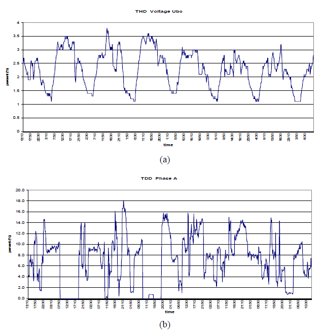
The power analyzer calculates voltage/current harmonic indices, voltage/current imbalance, voltage flicker, system frequency, and all power parameters for all three phases. Parameter calculation is done every cycle, and an average is taken over a 10 minute period. Fig. 1 shows a sample of the filed data for voltage and current THD in one of the test locations collected over one week. The test location is a 20 kV line which feeds a granite factory.
Fig.1. Filed data of a feeder supplying a granite factory (a) voltage THD (b) Current TDD
III. STATISTICAL ANALYSIS
For many PQ parameters, it is recommended that the Cumulative Probability (CP) of the captured data to be tabulated, and the value below which 95% of the measurement data lies is selected as the PQ index at the corresponding node [4]. This is called CP95% of that PQ parameter. This procedure is applied to all harmonic data as well as imbalance indices. Table 1 summarizes the results of statistical analysis of voltage THD in a granite factory.
TABLE I. Voltage THD analysis at a granite factory
.
IV. VOLTAGE RESULTS SUMMARY
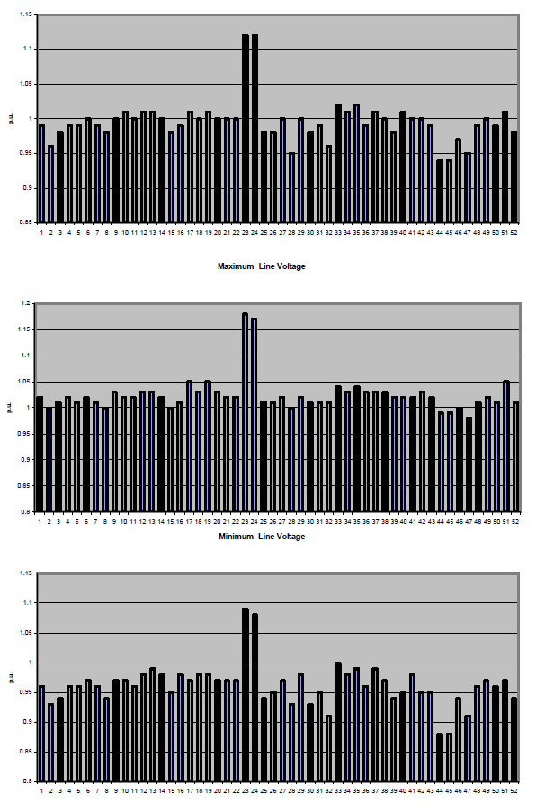
In this section, the study results are summarized. Fig. 2 shows average, maximum, and minimum rms voltage measured at different locations.
Fig.2. Voltage at 52 nodes
From Fig. 2, it can be seen that at 3.8% of the nodes in the distribution system, the maximum voltage level is beyond the maximum permissible 5% defined by the Iranian standard limits. At 25% of the locations, the minimum voltage is below the minimum permissible limit, i.e. 0.95 p.u..
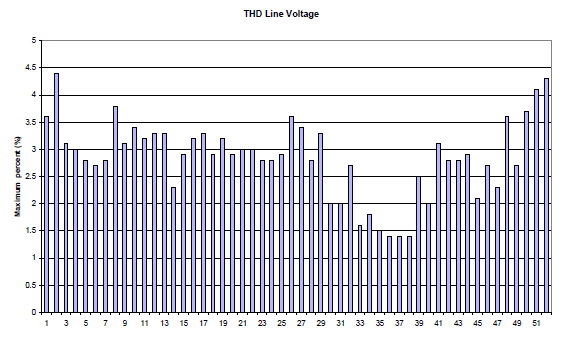
Figs. 3 and 4 depict voltage THD and the 5th harmonic at the tested nodes respectively. The results are compared against IEEE 519 Std. limits [4].
Fig.3. Voltage THD at 52 nodes
Fig.4. Voltage 5th harmonic at 52 nodes
It can be seen that the distribution system is IEEE 519 compliant in terms of voltage THD. However, as Fig. 4 shows, the level of the 5th harmonic is higher than IEEE 519 standard at some nodes. At 38.5 % of the cases, the 5th harmonic is not complaint with the standard. The same procedure is carried out to determine other harmonics as well.
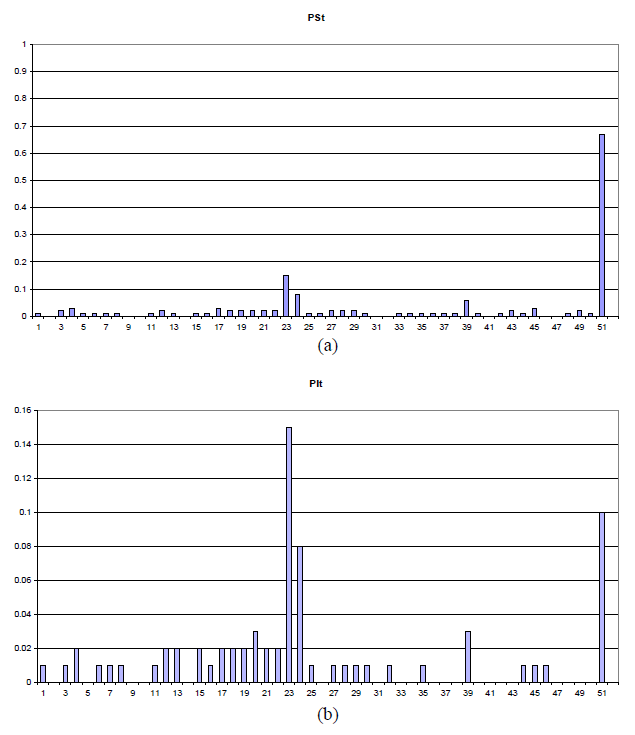
Flicker is the result of voltage fluctuation which is determined by the percentage of voltage change as well as its frequency. It is determined by short term and long term flicker, i.e. Pst and Plt, indices. The flicker level is compared against the level defined by IEC 61000-4-15 [5]. The power analyzer calculates only the Pst. Plt index is then calculated using the following equation:
.
Fig. 5 depicts the results for flicker determination. From Fig. 5, it can be concluded that the level of flicker is of no concern in the distribution system.
Fig.5. Voltage flicker a) Pst b) Plt
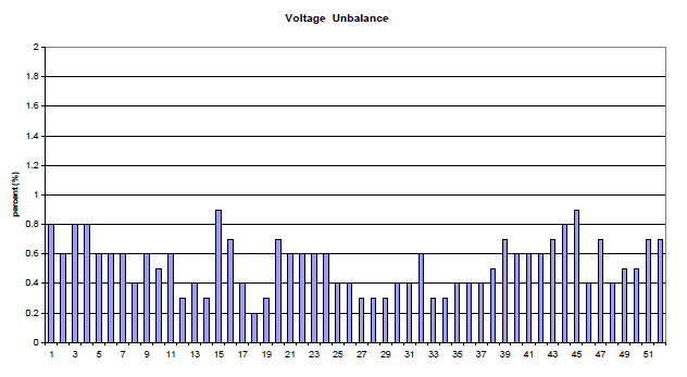
Fig. 6 shows the results of voltage imbalance in the distribution system. Based on IEEE 1159 Standard, the ratio of the negative sequence to the positive sequence is the imbalance ratio. To determine the imbalance index, the CP95 of the imbalance value calculated for each day, and the maximum CP95 is selected.
Fig.6. Voltage Imbalance
The maximum voltage imbalance was logged at node No. 15 which is 0.9. Since, the maximum permitted value is 2, therefore, the distribution system is fine with respect to voltage imbalance.
The other parameter which was investigated is the system frequency. Fig. 7 shows the maximum and minimum frequency at steady state operation. Based on Iranian standard, the maximum frequency deviation is 0.3 Hz. Therefore, at some moments, the system frequency drops below the minimum permissible threshold.
Fig.7. System maximum and minimum Frequency
V. CURRENT RESULTS SUMMARY
In this section, the quality of load current is investigated. Fig. 8 shows the results of the current harmonic pollution level. As it can be seen from this figure, at 13.5% of the locations, the TDD is out of limit. The results correspond to the CP95 index of the TDD.
Fig.8. Current TDD summary results
The analysis is extended to determine the pollution of load current in terms of individual harmonics. Fig. 9 depicts the results corresponding to the 3rd, 5th, 7th and 11th harmonics. The results indicate that the maximum pollution is related to the 5th harmonic. At 17.3% of the substations, at 20 kV, the 5th harmonic is beyond the permitted limit set by IEEE 519.
For the other harmonics, the results are as follows. At 1.9% of the locations, the 3rd and 7th harmonic are more than standard limits. At 11% of the locations, the 11th harmonic is out of standard limit.
Fig.9. Load individual harmonic levels at 52 nodes
Load power factor is also checked at the test locations. Fig. 10 shows the average power factor measured at the distribution transformer inputs. It can be seen that in most cases, the average power factor is acceptable.
Fig.10. Load average power factor
VI. ANALYSIS OF THE RESULTS AND STANDARD LIMITATION
The PQ survey in the utility under study indicate that the voltage quality is mostly within acceptable limits except for the 5th harmonic. However, the current distortion may be of concern at some locations. This conclusion is based on the CP95 limit which has the following shortcomings:
• The CP95 index is silent about the operating condition. In some cases, e.g. at light load conditions, the THD and TDD values may become larger than expected.
• The CP95 does not directly reflect the effect of harmonic on devices, e.g. extra heat in magnetic systems.
• The results show that the number of cases in which the 5th voltage harmonic level is more than standard is higher than that of the 5th current harmonic. This implies that in some cases, the load is injecting standard level of harmonics into the distribution system, however, the level of the voltage harmonic is not standard.
• The CP95 of current cannot be easily related to the CP95 of the voltage signal.
VI. DISCUSSION AND CONCLUSIONS
This paper presents the PQ analysis in a utility system. The analysis is based on IEEE standard limits. The study shows that the growth of nonlinear loads is propagating into the utility distribution system gradually. The 5th harmonic is becoming a concern in terms of standard limits. This problem has to be mitigated at load sites by using proper compensating devices, e.g. harmonic filters. However, the existing procedures have to change in a way to relate the pollution to system malfunction and costs more directly. There are shortcomings associated with the existing procedures and limits when it comes to three-phase unbalanced and non-sinusoidal conditions. At the moment, the quality of voltage at 20kV distribution level is acceptable considering IEEE and IEC standards. However, this cannot be guaranteed if the rate of increase of non linear loads does not change or counter measure actions are not taken in order to prevent power quality problems to propagate from load sites into distribution and transmission systems.
V. REFERENCES
[1] D. Chapman, “The cost of poor power quality”, Copper Development Association, March 2001. [2] G. W. Massey, “Estimation method for power system harmonic effect on power distribution transformer,” IEEE Transaction on Industry Applications, vol. 30, no. 2, pp. 485-489, 1994. [3] G.T. Heydt, R. Ayyanar, R. Thallam, “Power Acceptability”, IEEE Power Engineering Review, 2001. [4] Recommended Practices and Requirements for Harmonic Control in Electrical Power Systems, IEEE Standard 519-1992. [5] Flicker meter-functional and design specification, IEC Standard 61000-4-15, 1997
VIII. BIOGRAPHIES
Hossein Mokhtari was born in 1969 in Tehran, Iran. He received his B.Sc. degree in electrical engineering from Tehran University, Tehran, Iran in 1989. He worked as a consultant engineer for Electric Power Research Center (EPRC) in Tehran in dispatching projects. In 1994, he received his M.A.Sc. degree from University of New Brunswick, Fredericton, N.B., Canada. He obtained his Ph.D. degree in electrical engineering from the University of Toronto in 1998. He is currently an associate professor at Sharif University of Technology, Tehran, Iran. His research interests include power quality and power electronics.
Sasan Hasani was born in July 1976 in Orumieh. He received his B.Sc. in electrical engineering from Shaihd Abbaspour University, Tehran, Iran. He is currently a project engineer working in transmission and distribution network division of West Azarbayjan Regional Electric Company, Orumieh, Iran.
Masoud Masoudi was born in April 1951 in Orumieh. He received his B.Sc. in electrical engineering from Iran University of Science and Technology, Tehran, Iran. He obtained his masters degree in management from Orumieh University, Orumieh, Iran. He is currently the head of Engineering Department of West Azarbayjan Regional Electric Company.
Published by Michał PIEKARZ, Politechnika Warszawska, Instytut Elektroenergetyki ORCID: 0000-0003-1500-2634
Abstract. The article discusses the issues related to the influence of connecting wind turbines on the angular stability of the power system. Current plans for Poland’s energy transition, climate issues, and the most popular types of wind turbines used in the world were discussed. In the study part, the impact of replacing traditional generating units with wind turbine systems connected by converters on the angular stability of the New England test model was analysed.
Streszczenie. W artykule zostały omówione zagadnienia dotyczące wpływu przyłączania turbin wiatrowych na stabilność kątową systemu. Omówiono aktualne plany dotyczące transformacji energetycznej Polski, kwestie klimatyczne, a także najpopularniejsze rodzaje turbin wiatrowych, wykorzystywanych na świecie. W części badawczej przeanalizowano wpływ zastępowania tradycyjnych jednostek wytwórczych układami turbin wiatrowych przyłączanych przez przekształtniki na stabilność kątową modelu testowego systemu New England. (Analiza wpływu generacji wiatrowej na stabilność systemu elektroenergetycznego)
Słowa kluczowe: stabilność kątowa, generacja wiatrowa, inercja systemu elektroenergetycznego, analiza wartości własnych. Keywords: angular stability, wind generation, power system inertia, eigenvalue analysis.
Introduction
Along with the economically and technologically developing society, the arises issues will have to be solved in the next few years. Continuous economic development, and thus an increase in energy demand, will not be the only problem that power systems will be facing. The dynamics of the increase in electricity demand [1], climate change and excessive carbon dioxide emissions must be considered [2]. One of the solutions to the above problems can be renewable energy sources. The European Union’s climate and energy policy will, in general, strive for climate neutrality as early as 2050 [3].
One of the main pillars of this policy is, among others, changing the energy mix with an increased share of renewable sources [4].
Increasing number of generating units, connected to the system by converters may cause problems related to the stability or decreasing inertia of the power system [5]. The aim of this article is to present research on replacing traditional generating units with wind farms, as well as assessing their impact on the angular stability of the system.
Climate and energy
The climate and energy policy of the European Union (EU) has a fundamental impact on the national energy strategy, including the long-term vision of achieving the EU’s climate neutrality by 2050 [6,7]. Along with the dynamic economic development that Poland has been experiencing for 30 years, the demand and generation of energy is also increasing. In the case of gross domestic energy consumption, coal plays a central role in Poland – in 2018 it accounted for 46% of the share. Then petroleum (29%), natural gas (15%) and renewable energy sources (9%) [8].
At the same time, excessive carbon dioxide emissions in the electricity sector [1] and climate change around the world, cause the growth of generation from renewable energy sources (RES) [9].
Achieving the climate and energy goals by 2030 is extremely important to accomplish the required low emission energy transformation. In December 2020, the European Council approved targets to reduce net greenhouse gas emissions to at least 55% compared to 1990 levels [3].
The Energy Policy of Poland until 2040 (PEP2040) formulates the scope of the energy transformation in Poland. It specifies, among others, range of technology selection aimed at development of a low-emission power system. The key assumptions of the PEP2040 document regarding the power industry mention [6]:
• Increase in the share of RES in all sectors and technologies. In 2030, the share of RES in gross final energy consumption will be at least 23%, including: no less than 32% in electricity (mainly wind and PV); 28% in heating; 14% in transport (with a large contribution of electromobility).
• The installed capacity of offshore wind energy will be approx. from 5.9 GW in 2030 to approx. 11 GW in 2040.
Wind Energy in Poland
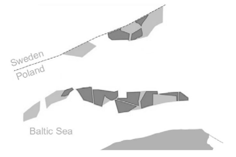
At the end of 2020, the installed capacity of onshore wind was 6347 MW [10]. Also in 2020, the act on supporting offshore wind farms was passed [7]. Subsequently, the European Commission approved the rules of public aid, and all the effort was dedicated on implementing regulations. It was all for the purpose of ensuring that electricity from offshore farms in the Baltic Sea will flow to customers by the end of 2025. The Fig. 1 shows the location of the offshore wind farms in the Polish part of the Baltic Sea, where the most important projects are marked with dark gray color [11].
Fig.1. Offshore wind farms locations on Polish Part of the Baltic Sea [11]
According to the PEP2040, two scenarios for wind farms in Poland have been proposed – base and ambitious scenario. The base scenario assumes that 10 GW of installed onshore and 5.9 GW of offshore capacity will be achieved by 2030, and 10 GW of onshore and 11 GW of offshore capacity by 2040. The ambitious scenario assumes 18 GW of installed capacity onshore and 5.9 GW at sea will be achieved by 2030, and 25 GW by 2040 on land and 14- 15 GW at sea. The wind energy for 2020 is as follows: 6.35 GW of installed capacity on land, 16 TWh of electricity production and 1239 installations [8,12].
Wind turbine types
The types of wind turbines that are used in currently operating wind farms are shown in Fig. 2. Variable speed wind turbines are equipped with DFIG (Doubly-fed Induction Generator) or full converter generators with PMSG (Permanent Magnet Synchronous Generator). This is due to the better control properties, compared with constant speed wind turbine generators (induction generators). In the case of DFIG generators, their advantage is that only 30% of the power flows through the circuit with the converter. In the case of a synchronous generator (PMSG), the converter must be sized for the full power of the generator. Synchronous generators are more efficient and have a simpler structure, but their cost is higher. In the case of DFIG generators, it is necessary to use additional protection systems against current surge in the event of damage.
Fig.2. Types of generators used in wind turbines: a) doubly-fed induction generator (DFIG), b) permanent magnet synchronous generator (PMSG).
Influence of wind farms on the dynamics of the power system
High penetration of a power-electronic connected generators, and therefore decommissioning of generation units with rotating masses, can decrease the system inertia. Traditional generation is based on large turbo or hydro generation units. These units make a significant amount of inertia in the system which is very important for maintaining power system stability. After a power loss, the resulting system frequency drop is delayed by rotating inertia of such generation units [5].
Renewable generation, such as Photo-voltaic systems and wind turbines, are connected through the power electronic devices. This way of connecting generation results in no additional inertia in the power system.
There is a concern that the rate of change of frequency (RoCoF) will increase, and the system stability will be endangered. On Fig 3, there are four elements with high impact on electrical power systems such as: extension of grids (which can affect inter-area oscillations), weather phenomena, large power flows and the market effects.
Then another factors must be considered such as load behaviour (e.g., inverters) and load control. These elements, together with decreasing inertia, can affect frequency behaviour and the value of the inter-area oscillations damping.
Fig.3. Map of interaction [5]
Model of the New England power system
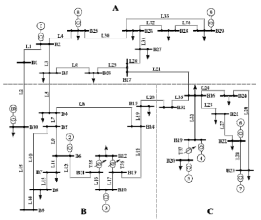
The analysis for this article was performed based on the 39 Bus New England System network model (Fig. 4). It is a simplified model of the high voltage network of the Northeast United States [13]. It consists of 39 nodes, 10 synchronous generators, 19 loads, 34 lines and 12 transformers. It uses a rated frequency of 60 Hz, and the highest voltage level is 345 kV. There are also voltages such as 230 kV, 138 kV and 16.5 kV. The G10 generator represents the interconnection of US and Canadian systems. The remaining generators are connected via transformers to the network.
Fig.4. New England power system [14,15]
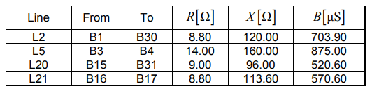
For the purposes of the research, in the field of interarea oscillations, the length of four lines in the model was increased by changing the basic parameters – resistance, reactance and susceptance. The following lines were extended: L2 connecting nodes B1 and B30, L5 – nodes B3 and B4, L20 – nodes B15 and B31 and L21 – nodes B16 and B17. The new parameters of the lines are presented in Table 1.
Table 1. Parameters of the modified line sections
.
Method and plan of the analysis
This article presents the results of the local angular stability analysis of the power system. The research was carried out in the Power Factory software. For this purpose, the modal analysis module was used to determine the eigenvalues, the oscillation frequencies, and the damping coefficients.
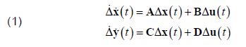
For small perturbations, the system can be expressed in linearized form as follows [16]:
.
where: Δ is the prefix which denotes a small deviation, A is the state or plant matrix, B is the control input matrix, C is the output matrix, D is the matrix, which defines the proportion of input which appears directly in the output.
The eigenvalues of the state matrix A determine the time domain response of the system to small disturbances. From state matrix A we can calculate the eigenvalues which can determine the stability of the system. For a complex pair of eigenvalues λ = σ ± jw , the real component gives the information about damping and the negative values represents a damped oscillations. The frequency oscillations f in Hz is given by:
.
and the damping ratio ξ is given by:
.
The research program was divided into the following cases:
• Case 1 – the basic model of the system with extended lines L2, L5, L20 and L21.
• Case 2 – in the basic model, the traditional G03, G07 and G09 generation units were replaced with wind generation units of the full-converter type.
• Case 3 – in the basic model, traditional generation units located in area C were replaced, i.e., G04, G05, G06 and G07 (Area C becomes non-inertia).
Additionally, the model from Case 3 investigated the effect of installing additional synchronous units along wind turbines.
The results of the analysis
a) Case 1
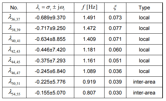
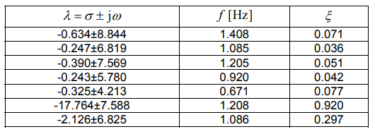
The research starts with the analysis of the basic case 1 i.e., identification of electromechanical oscillations. As part of this study, the eigenvalues related to local and inter-area oscillations were distinguished, as well as the oscillation frequencies and damping coefficients. The results for the Case 1 are presented in Table 2.
In the Case 1, eigenvalues related to inter-area oscillations were distinguished – 50, 51 and 54, 55. The generators G02 (50, 51) and G09 (54, 55) had a dominant share in these specific eigenvalues.
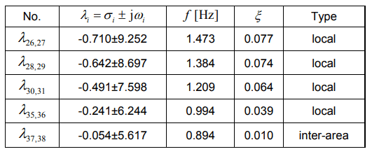
b) Case 2
In the Case 2, the synchronous generators G03, G07 and G09 were replaced by the wind generators. Compared to the Case 1, the Case 2 had eigenvalues related to interarea oscillations – 37, 38. In those eigenvalues, the interarea oscillations are dominated by the G10 generator, with the oscillation frequency slightly increased (from 0.807 to 0.894), and the damping factor decreased (from 0.030 to 0.010). The results for the Case 2 are presented in Table 3.
Table 2. The results for the Case 1
.
Table 3. The results for the Case 2
.
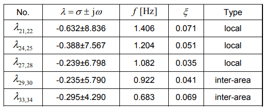
c) Case 3
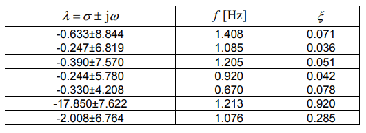
In Case 3, synchronous generators that were located in the C sector of the New England system were replaced by the wind turbines. In the Case 3, there are four eigenvalues related to inter-area oscillations – 29, 30 and 33, 34. As in the Case 1, the dominant generators in these eigenvalues are the generators G02 (29, 30) and G09 (33, 34), respectively. Compared to Case 1, the oscillation frequency related to the G02 generator remained practically the same (from 0.919 to 0.922) and for generator G09, the frequency oscillation decreased (from 0.807 to 0.683). The damping factor for generator G02 remained practically unchanged (0.039 to 0.041), while for G09, the damping factor increased (0.030 to 0.069). The results for the W3 variant are presented in Table 4.
Table 4. The results for the Case 3
.
d) Additional analysis for Case 3
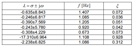
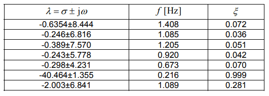
In the next part, the Case 3 was extended by four additional cases 3 (G4), 3 (G5), 3 (G6), and 3 (G7). In each of them, in the place of the synchronous generator replaced by the wind turbine, an additional inertia was introduced i.e., a synchronous source that would contribute to the system inertia.
The results of the Case 3 with additional inertia at the location of the generator G4 are presented in Table 5. Table 6 presents the results for the Case 3 with additional inertia at the location of the generator G5. Table 7 presents the results for the Case 3 with additional inertia at the location of the generator G6. Table 8 presents the results for the Case 3 with additional inertia at the location of the generator G7.
Table 5. The results for the Case 3 (G4)
.
Table 6. The results for the Case 3 (G5)
.
Table 7. The results for the Case 3 (G6)
.
Table 8. The results for the Case 3 (G7)
.
Compared to Case 3. the number of eigenvalues in the field of electromechanical oscillations increased by 4, while the effect of connecting an additional inertia had little impact on the eigenvalues of the system. However, a change can be seen in the case of eigenvalues related to the added inertia (last two rows). In the Case 3 (G5), a reduction in the oscillation frequency from approx. 1 Hz to 0.216 Hz can be noticed. The damping factors did not change much.
Summary
The article presents current issues related to renewable energy sources – energy transition, Poland’s energy policy until 2050, and the current state of wind energy. The issue of integration of renewable energy units connected to the system by converters was discussed.
The results of the local angular stability studies for various cases of replacing conventional sources with wind sources were presented. The tests were carried out on a model of the New England power system. The base model was modified, the length of four lines was increased. Then, three cases of research were proposed, in which traditional generating units were replaced by wind turbines. An analysis of connecting additional inertia at the wind farm location was also performed.
The obtained research results confirm that the transformation of the generation sector of the power system has an impact on the dynamics of the power system.
REFERENCES
[1] Rabiega W., Sikora P., Gąska J., CO2 Emissions Reduction Potential in Transport Sector in Poland and the EU Until 2050, 2019. [2] Luboińska B., Emisja gazów cieplarnianych. Wybrane zagadnienia dotyczące emisji CO2 w Polsce. Opracowanie tematyczne OT-683, Kancelaria Senatu, 2020. [3] Wolf S., Teitge J., Mielke J., Schütze F., Jaeger C., The European Green Deal — More Than Climate Neutrality, Intereconomics, vol. 56, no. 2, pp. 99–107, Mar. 2021. [4] Paska J., Surma T., Electricity generation from renewable energy sources in Poland, Renewable Energy, vol. 71, pp. 286–294, 2014. [5] Entso-E, Inertia and Rate of Change of Frequency (RoCoF), 2020. [6] Polityka Energetyczna Polski do 2040 r., 2021. [7] Minister Kurtyka on RES in the Polish energy mix, https://www.gov.pl/web/climate/minister-kurtyka-on-res-in-thepolish-energy-mix. [8] Ceglarz A., Polska Polityka energetyczna, 2020. [9] Marks-Bielska R., Bielski S., Pik K., Kurowska K., The importance of renewable energy sources in Poland’s energy mix, Energies, vol. 13, no. 18, 2020. [10] Urząd Regulacji Energetyki, https://www.ure.gov.pl/. [11] Polskie Stowarzyszenie Energetyki Wiatrowej, Przewodnik po systemie wsparcia dla morskich elektrowni wiatrowych na Bałtyku, 2020. [12] TPA Poland, Baker Tilly TPA, Lądowa energetyka wiatrowa w Polsce, Onshore wind energy in Poland – Raport, 2021. [13] Digisilent PowerFactory, 39 Bus New England System Manual. [14] Łukasz N., Sylwester R., Machowski J., Control Algorithm for UPFC Based on Non-linear Model of Power System, Electric Power Components and Systems, 47, ISSN 1532-5008, pp. 605-618, 2019 [15] Skwarski M., Robak S., Piekarz M., Polewaczyk M., MultiObjective Optimal Sizing of Shunt Braking Resistor for Transient State Improvement, IEEE Access, vol. 9, pp. 69127-69138, 2021. [16] Machowski J., Bialek J.W., Bumby J.R., Power System Dynamics Stability and control, Second Edition John Wiley&Sons, Chichester, 2008.
Autorzy: mgr inż. Michał Piekarz, Politechnika Warszawska, Wydział Elektryczny, Instytut Elektroenergetyki, ul. Koszykowa 75, 00-662 Warszawa, E-mail: michal.piekarz@ien.pw.edu.pl.
Source & Publisher Item Identifier: PRZEGLĄD ELEKTROTECHNICZNY, ISSN 0033-2097, R. 97 NR 11/2021
Published by Katarzyna GĘBCZYK, Andrzej Ł. CHOJNACKI, Łukasz GRĄKOWSKI, Kornelia BANASIK Kielce, University of Technology, Department of Power Engineering Basics
Abstract. The article presents the results of the analysis of the costs of losses at distributors and consumers of electricity, caused by failures of medium voltage overhead and cable power lines operated by domestic distribution companies. The components of failure costs were analyzed. Average values, standard deviations and confidence intervals for the mean value were also determined: The non-parametric verification of the costs analyzed was also carried out.
Streszczenie. W artykule przedstawiono wyniki analizy kosztów strat u dystrybutorów oraz odbiorców energii elektrycznej, spowodowanych awariami napowietrznych i kablowych linii elektroenergetycznych średniego napięcia eksploatowanych w krajowych spółkach dystrybucyjnych. Analizie poddano składniki kosztów awarii. Wyznaczono wartości średnie, odchylenia standardowe oraz przedziały ufności dla średniej. Dokonano także weryfikacji nieparametrycznej analizowanych kosztów. (Analiza porównawcza kosztów awarii linii napowietrznych i kablowych średniego napięcia)
Keywords: overhead MV lines, cable MV lines, reliability, power industry Słowa kluczowe: linie napowietrzne średniego napięcia, linie kablowe średniego napięcia, niezawodność, energetyka
Introduction
Over the last several dozen of years, in connection with, among others, Poland’s accession to the European Union, the interest in the problem of reliability of power systems has increased. The reason for this is the fact that even the shortest interruption results in dissatisfaction of electricity consumers and material losses. Correct and reliable operation of medium voltage grids is possible with reliable operation of individual network devices.
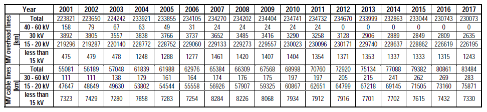
High reliability of operation of medium voltage lines allows to reduce the time of interruptions in power supply to customers, and thus to minimize the costs of losses resulting from the lack of power supply to customers. Medium voltage power lines are one of the most important elements of distribution networks. They enable the transmission of electricity at the most advantageous voltage values from the technical and economic point of view. Table 1 presents the lengths of medium voltage overhead and cable lines operated in the Polish power system in the years 2001 – 2017.
There have recently been many publications and studies indicating the need to quickly replace medium and low voltage overhead power lines with cable lines. Such actions are supposed to significantly increase the continuity of supply to customers from the commercial power grid. However, there are a number of doubts as to whether such measures are technically and economically justified. The technical aspect is discussed, among others, in publications [8, 9]. In this article the Authors deal with the economic part of this issue. They analyzed the costs of removing overhead and cable line failures, as well as the losses caused by the unreliability of these lines to the municipal electricity consumers.
The comments and conclusions contained in the article are of a debatable nature and in the intention of the Authors should provoke a polemic among all entities interested in the problem of continuity of electricity supply to consumers, whether the plans for universal cabling of Polish distribution networks are fully justified from the point of view of the cost of unreliability of these lines. In the case of cable lines, only lines with cross-linked polyethylene insulated cables were analyzed, as such cables are used in the execution of new investments. The article presents the results of a detailed statistical analysis of the individual components of the total unreliability costs of medium voltage overhead and cable lines incurred by energy distributors. Research was also carried out into the costs of losses incurred by municipal electricity consumers as a result of power cuts. The analysis was performed on the basis of economic and financial data of a power company and reliability data from observations in a large Polish distribution company, recorded over a period of 15 years. 1950 cases of medium voltage overhead line failures and 1350 cases of medium voltage cable line failures were considered. On this basis, average values of analyzed costs, standard deviations, confidence intervals for the mean value as well as minimum and maximum values were determined. Non-parametric verification was also carried out. Theoretical distributions of probability density of costs of losses at energy consumers and distributors were determined. All the analyses were carried out at the level of significance α = 0.05
Table 1. Lengths of medium voltage overhead and cable lines operated in the Polish power system [1]
.
The average value from sample t̄a was estimated using the method of the highest reliability, based on the formula [10]:
.
where: ¯Ka – mean value from the sample; K̇i– center of i-th class of the frequency distribution; ni – number of failures in the i-th class of the frequency distribution; n – total number of failures; k – number of classes of the frequency distribution.
The confidence interval for the mean is determined according to the formula [4, 10]:
.
where: ¯Ka – mean value from the sample; ua – value of a random variable U with a standardized normal distribution, determined for a given confidence coefficient 1-α from the normal distribution table; s – standard deviation from the sample calculated according to the formula:
.
Cost characteristics of losses in electricity distributors and consumers
The costs of losses incurred by electricity distributors are primarily related to the removal of failures and loss of profit due to non-delivery of electricity to consumers. These costs, together with the operating costs, reduce the company’s profit. The costs of removal of failures are the sum of at least a few components. These are mainly [4, 6]:
• costs of purchasing new equipment and materials; • operating costs of construction equipment, cable laboratory, etc.; • operating costs of fitters and other persons involved in repairing breakdowns; • costs of travel to the site of failure.
The cost of purchasing new equipment and materials is very diverse. Its value depends on the extent of the failure and the damaged device (component). The costs of equipment operation result from the fact that during the location of the failure or directly in the phase of its removal, specialist construction or power equipment is used, such as cranes, excavators, manlifts, drilling rigs, long-load trailers, cable laboratories and others. The cost of operation of each of these devices increases the total cost of equipment operation. Regardless of whether specialist equipment is used, a group of fitters from the distribution company must always arrive at the location of the failure. This entails the cost of travel of a power emergency service car. Removing failures in power systems involves considerable human labor input. This labor results both from the need to operate specialist equipment and from the need to perform many tasks manually or only with simple fitting tools. The work of the workers removing the failure involves remuneration that must be provided to them. Labor costs are the higher the more time it takes to remove the failure and the more people work on it.
As a result of a failure of power equipment, consumers do not receive electricity. The result is a loss of profit for the distribution and trade companies. The costs of lost profit can be determined on the basis of the formula [4, 7]:
.
where: kjuz – unit profit loss indicator in PLN/MWh, ΔA – amount of electricity not delivered to consumers as a result of failure, determined on the basis of the active power load diagram P = f(t) of a given network.
Ultimately, the total cost of losses at the distributor can be determined from the formula [4, 7]:
.
where: Kaw – cost of failure, Kmiu– cost of purchase of new materials and equipment, Ksprz – cost of equipment operation, Kpm – cost of fitters’ labor, Kd – cost of emergency service and construction equipment’s travel to the site of failure, Kuz – cost of lost profit.
In the next part of the article the results of a detailed statistical analysis of the costs occurring in the formula (5), in case of medium voltage overhead and cable line failures are presented.
Costs of losses at electricity distributors in case of medium voltage overhead and cable line failures
1. Costs of purchasing new materials and equipment
On the basis of empirical data, statistical parameters characterizing the costs of purchase of materials Kmiuin case of medium voltage overhead and cable line failures were determined. The values obtained are shown in Table 2.
Table 2. Statistical indicators characterizing the costs of purchase of materials in case of medium voltage overhead and cable line failures
.
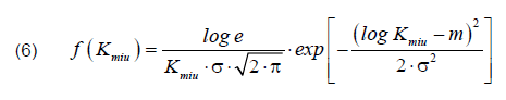
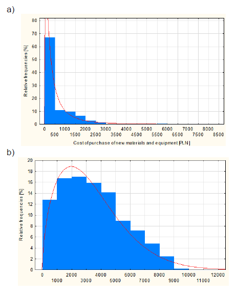
A correspondence analysis of the empirical distribution of the costs of purchase of new equipment and materials with the selected theoretical model was carried out. A hypothesis was put forward that the theoretical distribution of probability density of the cost of purchase of equipment and materials in the event of failure of medium voltage overhead lines is a log-normal distribution of the following form [6, 17, 18]:
.
where: m – expected value of the log Kmiu random variable, σ – standard deviation of the log Kmiu random variable.
The values of distribution parameters (6) determined using the Statistica package for MV overhead lines are: m = 5.7900, σ = 1.2763.
A hypothesis was put forward that the theoretical distribution of probability density of the cost of purchase of equipment and materials in the event of failure of medium voltage cable lines is a Weibull distribution of the following form [6, 17, 18]:
.
where: b – scale parameter, v – shape parameter. The values of distribution parameters (7) determined using the Statistica package for MV cable lines are: m = 3798.99, v = 1.5608.
Empirical and theoretical functions of probability density of purchase costs of materials and equipment are presented in Figure 1.
Fig.1. Empirical and theoretical functions of probability density of purchase costs of new materials and equipment in case of failure of: a) MV overhead lines, b) MV cable lines
2. Equipment operation costs
On the basis of empirical data, statistical parameters characterizing the costs of equipment operation Ksprz in case of removing medium voltage overhead and cable line failures were determined. The values obtained are shown in Table 3.
Table 3. Statistical indicators characterizing the costs of equipment operation in removing failures of medium voltage overhead and cable lines
.
A correspondence analysis of the empirical distribution of the costs of equipment operation with the selected theoretical model was carried out. On the basis of empirical data, a hypothesis was assumed that the theoretical distributions of probability densities of equipment operation costs in the removal of medium voltage overhead and cable line failures are log-normal distributions.
The values of distribution parameters (6) determined using the Statistica package are for MV overhead lines: m = 6.2504, σ = 0.8577 and for MV cable lines: m = 7.3038, σ = 1.1267.
Empirical and theoretical functions of probability density of equipment operation costs are presented in Figure 2.
Fig.2. Empirical and theoretical functions of probability density of equipment operation costs in case of failure removal of: a) MV overhead lines, b) MV cable lines
3. Fitters’ labor costs
On the basis of empirical data, statistical parameters characterizing the costs of labor of fitters and other people in removing medium voltage overhead and cable line failures were determined. The obtained results are presented in Table 4.
Table 4. Statistical indicators characterizing the costs of fitters’ labor in removing failures of medium voltage overhead and cable lines
.
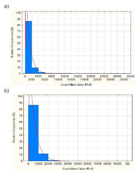
On the basis of empirical data, a hypothesis on the exponential distribution of the costs of fitters’ labor for the removal of medium voltage overhead and cable line failures was assumed. The function of probability density of exponential distribution is determined by the formula:
.
The value of the coefficient λ is in this case equal to the reciprocal of the mean value from the sample:
.
Determined values of distribution parameters are in case of MV overhead line failure λ = 852.4·10-6, and in case of MV cable line failure λ = 185.6·10-6.
Empirical and theoretical functions of probability density of fitters’ labor costs in case of removal of MV overhead and cable line failures are presented in Figure 3.
Fig.3. Empirical and theoretical functions of probability density of fitters’ labor costs in case of failure removal of: a) MV overhead lines, b) MV cable lines
4. Costs of travel to the site of failure
On the basis of empirical data, statistical parameters characterizing the costs of travel to the site of failure in case of removing medium voltage overhead and cable line failures were determined. The obtained results are presented in Table 5.
Table 5. Statistical indicators characterizing the costs of travel to the site of failure in case of removing medium voltage overhead and cable line failures
.
On the basis of empirical data, a hypothesis was assumed that the theoretical distributions of the probability densities of the costs of travel to the site of failure in case of overhead and cable line failures are Weibull distributions.
The values of distribution parameters (7) determined using the Statistica package are for MV overhead lines: b = 79.2174, v = 1.2094 and for MV cable lines: b = 69.3839, v = 1.5756.
Empirical and theoretical functions of probability density of the value of the cost of travel to the site of failure of MV overhead and cable lines are presented in Figure 4.
Fig.4. Empirical and theoretical functions of probability of costs of travel to the site of failure in case of failure removal of: a) MV overhead lines, b) MV cable lines
5. Costs of lost profit
On the basis of empirical data concerning the amount of electricity not delivered to consumers, statistical parameters characterizing the costs of lost profit as a result of failures of medium voltage overhead and cable lines were determined. The obtained results are presented in Table 6.
Table 6. Statistical indicators characterizing the costs of lost profit in case of medium voltage overhead and cable line failures
.
On the basis of empirical data, a hypothesis on the exponential distribution of the costs of lost profit for the removal of medium voltage overhead and cable line failures was assumed. Determined values of distribution parameters for failure of MV overhead lines are λ = 0.0021, and for failure of MV cable lines: λ = 0.0066.
Empirical and theoretical functions of probability density of lost profit costs in case of MV overhead and cable line failures are presented in Figure 5.
Fig.5. Empirical and theoretical functions of probability density of lost profit costs in case of failure of: a) MV overhead lines, b) MV cable lines
6. Total costs of losses for electricity distributors
On the basis of empirical data, statistical parameters characterizing the total cost of losses for distributors as a result of medium voltage overhead and cable line failures were determined. The obtained results are presented in Table 7.
Table 7. Statistical indicators characterizing the total cost of losses for energy distributors in case of medium voltage overhead and cable line failures
.
On the basis of empirical data, a hypothesis on lognormal distribution of costs of losses at energy distributors in case of medium voltage overhead and cable lines failures was assumed. Determined values of distribution parameters for MV overhead lines are: m = 7.7179, σ = 0.7678 and for MV cable lines: m = 8.9634, σ = 1.0226.
Empirical and theoretical functions of probability density of costs of losses at distributors in case of MV overhead and cable line failures are presented in Figure 6.
Fig.6. Empirical and theoretical functions of probability density of costs of losses at energy distributors in case of failure of: a) MV overhead lines, b) MV cable lines
Costs of losses at household consumers caused by discontinuity of power supply
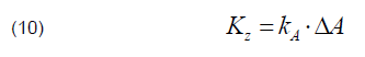
The cost of losses at municipal power consumers can be estimated on the basis of the formula:
.
where: kA – economic equivalent of undelivered electricity in PLN/kWh, ΔA – amount of electricity undelivered to consumers as a result of a failure in kWh.
On the basis of the conducted analyses and calculations, the authors of the publication [3] obtained the value of the unit economic equivalent of undelivered electricity kA = 21.48 PLN/kW·h. Based on the above indicator and empirical data from the operation of medium voltage lines, statistical parameters characterizing the costs of losses at energy consumers in case of medium voltage overhead and cable line failures were determined. The issue of the costs of losses at municipal consumers is described in more detail in publications [5, 6, 12]. The statistical indicators obtained in the analysis are presented in Table 8.
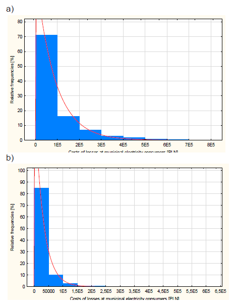
On the basis of empirical data, a hypothesis on the exponential distribution of costs of losses at energy consumers in case of medium voltage overhead and cable lines failures was assumed. Determined values of distribution parameters for failure of MV overhead lines are λ = 11.5·10-6, and for MV cable lines: λ = 33.6·10-6.
Table 8. Statistical indicators characterizing the costs of losses for energy consumers in case of medium voltage overhead and cable line failures
.
Empirical and theoretical functions of probability density of costs of losses at consumers in case of medium voltage overhead and cable line failures are presented in Figure 7.
Fig.7. Empirical and theoretical functions of probability density of costs of losses at energy consumers in case of failure of: a) MV overhead lines, b) MV cable lines
Conclusions
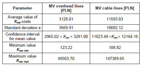
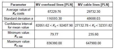
Table 9 presents the results of statistical analysis of average costs of unreliability of medium voltage overhead and cable lines.
Table 9. Average values of costs of losses at energy distributors resulting from medium voltage overhead and cable line failures
.
Figure 8 shows the share of individual components in the total cost of failure. Analyzing the parameters obtained as a result of the analysis, characterizing the costs of losses at distributors due to medium voltage overhead and cable line failures, it should be noted that the average costs of removing failures are higher for cable lines. In the case of removing cable line failures, compared to removing overhead line failures, the costs of equipment operation, fitters’ labor and travel to the site of failure are higher.
The largest part in the total costs are the costs of fitters’ labor and the costs of equipment operation. The share of fitters’ labor costs is about 37.50% in case of overhead line failures and about 46.47% in case of cable line failures. The share of equipment operation costs, in turn, is about 25.13% of medium voltage overhead line failure costs and 21.67% of cable line failure costs.
The cost of travel of power emergency service and mechanical equipment to the site of failure is similar for both overhead and cable lines.
Fig.8. Shares of individual components in total costs of removal of failures of: a) MV overhead lines, b) MV cable lines
In field networks, i.e. overhead lines, the share of lost profit costs is higher and amounts to approximately 15.03% of all the failure removal costs. For urban networks, i.e. cable lines, the share of lost profit costs is about 1.31%. This is due to the longer duration of supply interruptions in rural areas, which results in a higher value of electricity not supplied to consumers, which in turn determines the lost profit costs. This time also affects the average costs of losses at household consumers caused by discontinuity of power supply. In case of failures of MV overhead lines they are greater and amount to 87.229,76 PLN, and in case of failure of cable lines 29.732,30 PLN.
The total average cost of losses at energy distributors per one failure is PLN 3.128.01 for medium voltage overhead lines and PLN 11.593.83 for medium voltage cable lines. The total costs incurred by the electricity distributor during the considered 15-year period, i.e. in 1950 cases of overhead line failures, amounted to PLN 6.084.897, and in 1350 cases of cable line failures – PLN 15.824.984. This results in annual unreliability costs of PLN 405.659,80 for overhead lines and PLN 1.054.998,93 for cable lines.
According to the authors, the decision on the widespread cabling of MV distribution networks is advantageous for consumers, because it will result in shorter power supply interruption times and ultimately lower costs of losses caused by discontinuity of power supply. For distribution companies, however, this entails more than doubling the cost of unreliability related losses. Therefore, it seems pointless to replace further overhead lines with cable lines only in order to achieve the assumed network cabling index and to improve the SAIDI and SAIFI indexes. Even in the case of lower intensity of damage, cable lines generate (due to high costs of removing a single failure) much higher total unreliability costs compared to overhead lines. The only aspect of the economic and financial analysis in favor of cabling distribution networks is the cost of losses at municipal electricity consumers. These costs, for consumers supplied from overhead lines, are almost three times higher than for consumers supplied from cable networks. However, it should be taken into account that such a situation results primarily from the possibility of reserving the power supply to consumers, which possibility is much greater in urban networks, where cable lines prevail, than in field networks, where overhead lines prevail.
REFERENCES
[1] Agencja Rynku Energii S.A., Statystyka Elektroenergetyki Polskiej 200 – 2017, Warszawa 2001 – 2018 [2] Banasik K., Chojnacki A. Ł., Effects of unreliability of electricity distribution systems for municipal customers in urban and rural areas, Przegląd elektrotechniczny Nr 05/2019, p. 179-183 [3] Banasik K., Chojnacki A. Ł., Skutki gospodarcze niedostarczenia energii elektrycznej do odbiorców komunalnobytowych. Przegląd Elektrotechniczny Nr 3/2018, p. 181-187 [4] Chojnacki A. Ł., Analiza niezawodności eksploatacyjnej elektroenergetycznych sieci dystrybucyjnych. Wydawnictwo Politechniki Świętokrzyskiej, Kielce 2013 [5] Chojnacki A. Ł., Analiza skutków gospodarczych niedostarczenia energii elektrycznej do odbiorców indywidualnych. Wiadomości elektrotechniczne Nr 09/2009, p. 3-9 [6] Chojnacki A. Ł., Chojnacka K. J.: Niezawodność elektroenergetycznych sieci dystrybucyjnych. Wydawnictwo Politechniki Świętokrzyskiej, Kielce 2018 [7] Chojnacki A. Ł., Koszty strat u dystrybutorów oraz odbiorców energii elektrycznej spowodowane zawodnością układów uziomowych eksploatowanych w stacjach elektroenergetycznych SN/nn. INPE Informacje o normach i przepisach elektrycznych Nr 194-195 listopad-grudzień 2015, p. 46-58 [8] Chojnacki A. Ł., Analiza wskaźników oraz właściwości niezawodnościowych elektroenergetycznych linii napowietrznych i kablowych średniego napięcia. Wybór optymalnego wariantu linii w kontekście zapewnienia ciągłości zasilania odbiorców. XXII Konferencja Naukowo-Techniczna Bezpieczeństwo Elektryczne ELSAF 2019, Karpacz, 24-27.09.2019, p. 141-152 [9] Chojnacki A. Ł., Kablowanie sieci dystrybucyjnych średniego i niskiego napięcia jako metoda zwiększania niezawodności zasilania odbiorców energią elektryczną. XXII Konferencja Naukowo-Techniczna Bezpieczeństwo Elektryczne ELSAF 2019, Karpacz, 24-27.09.2019, p. 153-163 [10] Greń J., Modele i zadania statystyki matematycznej. PWN, Warszawa, 1982 [11] Horak J., Popczyk J., Eksploatacja elektroenergetycznych linii rozdzielczych. Warszawa, WNT 1985 [12] Kowalski Z., Niezawodność zasilania odbiorców energii elektrycznej. Wydawnictwo Politechniki Łódzkiej, Łódź, 1992 [13] Kujszczyk S. i in., Elektroenergetyczne sieci rozdzielcze. Warszawa, PWN 1994 [14] Lesiński S., Niezawodność urządzeń elektrycznych. Wydawnictwo Politechniki Łódzkiej, Łódź, 1989 [15] Paska J., Niezawodność systemów elektroenergetycznych. Oficyna Wydawnicza Politechniki Warszawskiej, Warszawa, 2005 [16] Popczyk J., Modele probabilistyczne w sieciach elektroenergetycznych. Warszawa, WNT 1991 [17] Sozański J., Niezawodność i jakość pracy systemu elektroenergetycznego. Warszawa, WNT 1990 [18] Sozański J., Niezawodność zasilania energią elektryczną. WNT, Warszawa 1982 [19] Wróblewski Z., Siwak P., Trwałość eksploatacyjna elektroenergetycznych linii kablowych średnich napięć. Wiadomości Elektrotechniczne Nr 9/2007, p. 74-76
Authors: M.Sc. Eng. Katarzyna Gębczyk, Prof. PhD Eng. Andrzej Ł. Chojnacki, M.Sc. Eng. Łukasz Grąkowski, M.Sc. Eng. Kornelia Banasik, Kielce University of Technology, Faculty of Electrical Engineering, Automatic Control and Computer Science, Department of Energy Basics, Poland, kgebczyk@tu.kielce.pl, a.chojnacki@tu.kielce.pl, lgrakowski@tu.kielce.pl, k.banasik@tu.kielce.pl
Source & Publisher Item Identifier: PRZEGLĄD ELEKTROTECHNICZNY, ISSN 0033-2097, R. 96 NR 10/2020. doi:10.15199/48.2020.10.14
Published by 1. Stanislaw CZAPP, 2. Daniel KOWALAK, Gdańsk University of Technology ORCID: 1. 0000-0002-1341-8276; 2. 0000-0001-9610-9884
Abstract. The scope of the verification of low-voltage systems covers the earth fault loop impedance measurement. This measurement is usually performed with the use of low-value current meters, which force a current many times lower than the one occurring during a real short-circuit. Therefore, the international standard recommends consideration of the increase of resistance of conductors with the increase of temperature, which may occur during short-circuits. This paper analyses the temperature rise of the conductors during short-circuits, taking into account the let-through energy of protection devices. The analysis has shown that in typical circuits the temperature rise of conductors is not significant.
Streszczenie. W ramach kontroli stanu instalacji niskiego napięcia wykonuje się pomiar impedancji pętli zwarciowej wymuszając prąd znacznie mniejszy niż występujący podczas rzeczywistego zwarcia. Norma dotycząca sprawdzania instalacji niskiego napięcia zaleca, aby w przypadku pomiarów małym prądem, w temperaturze pokojowej, uwzględnić fakt, że podczas zwarcia temperatura i rezystancja przewodów może wzrosnąć, co zaostrza warunek skuteczności ochrony przeciwporażeniowej. W artykule przeanalizowano, w jakim stopniu może wzrosnąć temperatura przewodów podczas zwarć przy uwzględnieniu całki Joule’a wyłączania zabezpieczeń nadprądowych. Z analizy wynika, że wzrost ten jest niewielki. (Wpływ energii przenoszonej przez zabezpieczenia nadprądowe na wzrost temperatury przewodów podczas zwarć).
Keywords: conductors resistance, let-through energy, overcurrent protection, short-circuit. Słowa kluczowe: rezystancja przewodów, energia przenoszona, zabezpieczenie nadprądowe, zwarcie.
Introduction
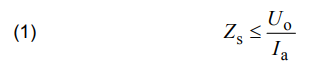
Earth faults both in high- and low-voltage systems may introduce an electric shock hazard. Every safety system, including a system of protection against electric shock, should fulfil at least the (n – 1) condition, i.e. the protection is ensured in case of the first fault (usually an insulation fault). In low-voltage systems, the most popular method of protection in case of a fault (protection against indirect contact) is the automatic disconnection of supply. The line-to-earth short-circuit current should be high enough to initiate tripping of the disconnecting device (circuit-breaker, fuse or residual current device) within the time specified in standard PN-HD 60364-4-41 [1]. This short-circuit current value depends on the value of the loop impedance of the faulty circuit. In order to achieve the effectiveness of protection against electric shock by automatic disconnection of supply, the following condition has to be fulfilled:
.
where: Zs – is the earth fault loop impedance (TN-type systems) determining the value of the line-to-earth (earth fault) current; Uo – is the nominal line-to-earth voltage; Ia – is the current causing the automatic operation of the disconnecting device within the specified time [1].
The effectiveness of protection against electric shock is required to be confirmed during the initial and periodic verification of low-voltage electrical installations [2-7]. The scope of this verification is included in standard PN-HD 60364-6 [8]. According to this standard, in TN-type systems (the most common), where possible, the measurement of the earth fault loop impedance is recommended to be carried out.
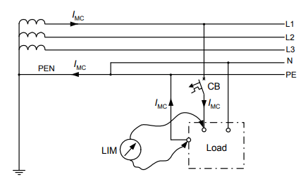
In practice, the loop impedance is measured with the use of the artificial short-circuit method. This method is utilized by the meters widely accessible in the market. During the measurement, the testing current IMC is forced (Fig. 1), and its value is from milliamps up to several hundred amps – it depends on the type of the meter.
Standard PN-HD 60364-6 [8] informs that consideration of the increase of the resistance of the conductors with the increase of temperature is recommended. For a relatively high value of the temperature of the conductors (in effect it gives a relatively high resistance), the earth fault current can be too low to initiate tripping of the protection device. It is written in this standard (Annex D – informative) that in the case of the measurement at room temperature, with the use of low-current methods (a practically negligible increase of the temperature of the conductors), the measured earth fault loop impedance in TN systems should satisfy the following dependence:
.
where: Zsm – is the measured earth fault loop impedance.
Such a dependence makes that conditions for effective protection against electric shock are clearly more rigorous (coefficient 2/3). Thus, according to the standard [8], when the measured impedance Zms exceeds the value described by (2), the more detailed calculation should be performed. In particular, the let-through energy of the protective device installed in the tested circuit should be taken into account.
Fig.1. Earth fault loop impedance measurement in a TN-C-S low voltage system; LIM – loop impedance meter, CB – circuit-breaker, IMC – measuring current
This paper covers the effect of the let-through energy of the protective device on the real increase of the conductors/cables temperature in case of short-circuits (earth faults). Results of the laboratory test of the let-through energy of selected miniature circuit-breakers and fuses are presented. On the base of this laboratory test and data delivered by the manufacturers of the overcurrent protection devices, the temperatures of conductors, in case of an earth fault, are calculated for an example electrical installation.
Resistance of conductors vs. their temperature
Resistance of conductors Rc and in consequence the loop impedance Zs (Zsm) given by (1) and (2), strictly depends on the conductors’ temperature. The resistance can be calculated according to:
.
where: l – is the length of the conductor; γx – is the conductivity of the conductor in temperature x; s – is the cross-sectional area of the conductor.
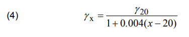
The conductivity γx in the temperature x is calculated in the following way:
.
where: γ20 – reference conductivity of the conductor (in 20 °C); x – given temperature of the conductor.
For commonly used PVC-insulated cables/conductors, the permissible continuous temperature is equal to 70 °C. In this temperature, the resistance of conductors is higher by 20% than in 20 °C:
.
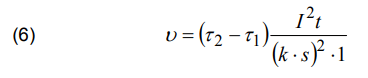
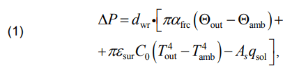
From the point of view of the effectiveness of the automatic disconnection of supply, it is important to evaluate the real temperature rise of the conductors during a short-circuit. The temperature rise v can be evaluated according to the following dependence [9]:
.
where: 𝜏1 – is the temperature of the conductor before a short-circuit; 𝜏2 – is the max permissible temperature of the conductor in the case of a short-circuit; I2t – is the let-through energy of the protective device; k – is the max permissible current density in the conductor (within 1 second); s – is the cross-sectional area of the conductor.
For a given type of a cable/conductor, the temperatures 𝜏1 and 𝜏2 as well as parameters k and s are known. The Joule integral (let-through energy) I2t of the protection device can be derived from manufacturers data, but the authors performed also a laboratory test to find out the real values of this parameter.
Results of the laboratory test and calculations
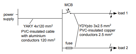
Figure 2 presents the structure of the analyzed example installation. It is assumed that the single-phase loads are supplied via PVC-insulated power cable having aluminium conductors (120 mm2) and PVC-insulated copper conductors (2.5 mm2). The first final circuit is protected by a miniature circuit-breaker (MCB) and the second by a fuse.
Fig.2. Structure of the analyzed electrical installation; MCB – miniature circuit-breaker
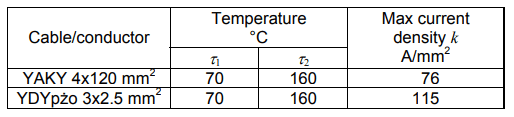
Based on the diagram from Fig. 2, the characteristic parameters of the power cable and final circuits’ conductors are as in Table 1.
Table 1. Parameters of the analyzed cable/conductors
.
In the investigation of the circuit marked “load 1”, the following types of the MCBs have been taken into account: B16, C16 and D20. The MCBs B16 and C16 are the most common types installed in final circuits. Also, the conductor of the cross-sectional area 2.5 mm2 (Fig. 2) is very popular in low-voltage final circuits.
First, as an example, the temperature rise of the conductor during a short-circuit has been evaluated on the base of the manufacturers’ data for the MCB of B16 type. Such data are presented in Fig. 3.
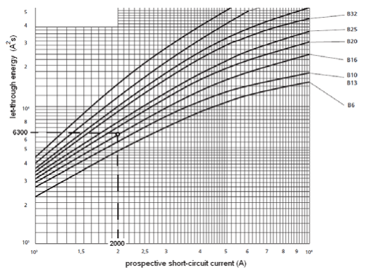
Fig.3. Maximum let-through energy of B-type circuit-breakers declared by the manufacturer [10]; the marked value of the let-through energy (6300 A2s) for a circuit-breaker B16 and a prospective short-circuit current 2 kA
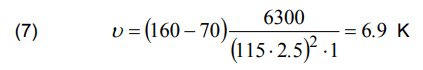
For a prospective short-circuit current equal to 2 kA, the value of the B16 MCB let-through energy is equal to 6300 A2s (Fig. 3). According to (6) and Tab. 1, it gives the temperature rise of the conductor YDYpżo 3×2.5:
.
For the cable YAKY 4×120, the temperature rise is as follows:
.
One can see that the temperature of the conductor YDYpżo 3×2.5 increases only slightly. In case of the cable YAKY 4×120, the increase is completely negligible.
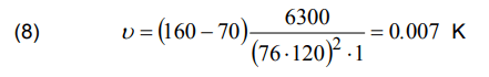
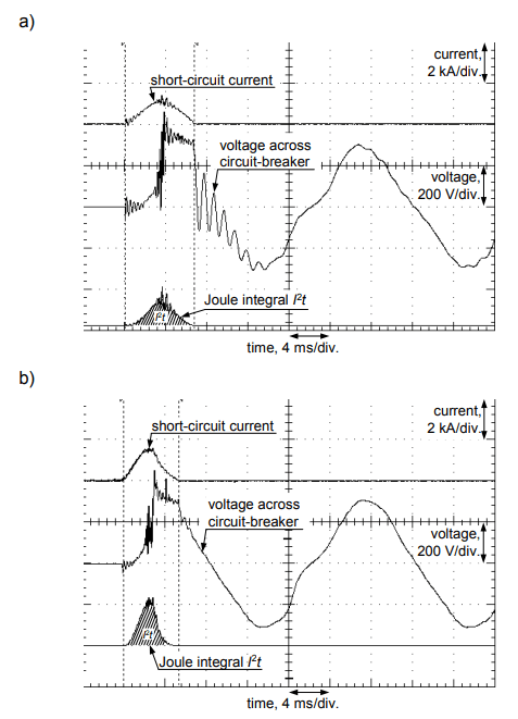
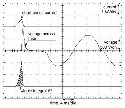
In order to check the real temperature rise, the laboratory test of the MCBs let-through energy has been carried out. Figures 4, 5, and 6 present results of this test for the MCBs B16, C16 and D20 respectively. The process of current breaking and the let-through energy value have been verified for prospective short-circuit currents 1 kA and 2 kA. Results of the temperature rise calculation, for data obtained from the laboratory test, are presented in Table 2.
Fig.4. Oscillograms of the real short-circuit current, voltage drop as well as Joule integral (let-through energy) during breaking of current by a circuit-breaker B16, for the value of a prospective short-circuit current: a) 1 kA (3.3 kA2s), b) 2 kA (3.3 kA2s)
Fig.5. Oscillograms of the real short-circuit current, voltage drop as well as Joule integral (let-through energy) during breaking of current by a circuit-breaker C16, for the value of a prospective short-circuit current: a) 1 kA (3.5 kA2s), b) 2 kA (4.2 kA2s)
Fig.6. Oscillograms of the real short-circuit current, voltage drop as well as Joule integral (let-through energy) during breaking of current by a circuit-breaker D20, for the value of a prospective short-circuit current: a) 1 kA (5.6 kA2s), b) 2 kA (6.5 kA2s)
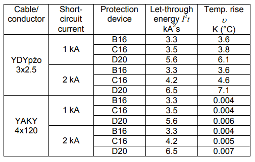
Table 2. Temperature rise of the cable/conductors in circuits protected by MCBs
.
If one compares the value of the maximum let-through energy for the MCB B16 derived by the manufacturer (Fig. 3: I2t = 6300 A2s, for 2 kA) with the let-through energy obtained during the laboratory test (Fig. 4b: I2t = 3300 A2s, for 2 kA), it is seen that the latter is almost two times lower. It gives only the 3.6 K temperature rise of the conductor YDYpżo 3×2.5 in case of a short-circuit with current 2 kA. The temperature rise of the cable YAKY 4×120 is – obviously – negligible (0.004 K). For other MCBs (C16 and D20) the temperature rise of the conductor YDYpżo 3×2.5 is maximum around 7 K and for the cable YAKY 4×120 is close to 0 K.
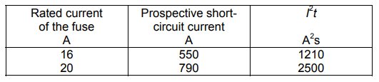
Even a lower temperature rise is expected in the circuit marked “load 2” (Fig. 2) protected by a fuse. In the investigation, the following general type fuses are taken into account: gG16 and gG20. If the normative maximum values of the let-through energy I2t are considered (Tab. 3), the temperature rise of the conductor YDYpżo 3×2.5 protected by a fuse gG16 (I2t = 1210 A2 s) is equal to 1.32 K (Tab. 4). This temperature rise is valid for both analyzed values of the prospective short-circuit currents 1 kA and 2 kA because the let-through energy is approx. constant (from 550 A onwards for gG16 – see Tab. 3). In the case of the cable YAKY 4×120, the temperature practically does not change the value (0.0013 K).
Table 3. Maximum let-through energy I2t of the gG fuses (IEC) [11]
Table 4. Temperature rise of the cable/conductors in circuits protected by gG fuses
.
Fig.7. Oscillograms of the real short-circuit current, voltage drop as well as Joule integral (let-through energy) during breaking of current by a fuse gG16, for the value of a prospective short-circuit current 1 kA (402 A2s)
Calculation of the temperature rise on the base of the selected manufacturer data (“ETI”, Tab. 4) enables to say that gG16 fuses have let-through energy not higher than 1060 A2 s, what is clearly lower than the max normative value (1210 A2 s – see. Tab. 3). This value also gives a very small increase in the temperature of the conductor YDYpżo 3×2.5 (1.15 K). A laboratory test of the fuses shows (“Lab”, Tab. 4) that in practice the let-through energy can be significantly lower than the manufacturer declaration (positive effect). Example oscillograms obtained from the testing of a fuse are presented in Fig. 7.
From the above-conducted calculations performed for the example electrical installation, with components having typical parameters, it can be determined that in the case of short-circuits, the temperature rise of the final conductor is relatively low and the temperature rise of the cable in a distribution circuit is practically negligible. This is due to the positive effect of the protection devices in terms of letthrough energy. Thus, during the earth fault loop impedance measurement, the safety margin presented by the expression (2) is too restrictive. Instead of the 2/3 value, this margin is acceptable to be expressed by the value around 0.90÷0.95.
Conclusions
Analysis of the values of the let-through energy of the protection devices, which are installed in typical low-voltage final circuits shows that the coefficient 2/3 included in the expression (2) gives too restrictive conditions in terms of the effectiveness of automatic disconnection of supply. Fortunately, this expression is only informative (not obligatory), and it is easy to prove that in the case of a short-circuit the temperature rise and resistance rise of the conductors are practically insignificant.
REFERENCES
[1] PN-HD 60364-4-41:2017-09 Low-voltage electrical installations – Part 4-41: Protection for safety – Protection against electric shock [2] Neitzel D.K., Electrical Safety Update – OSHA 29 CFR 1910.269 and NFPA 70E®-2015 Revisions, IEEE Industry Applications Society Annual Meeting, Addison, TX, USA, (2015), 1-6 [3] Roskosz R., Musiał E., Czapp S., A method of earth fault loop impedance measurement without unwanted tripping of RCDs, Progress in Applied Electrical Engineering (PAEE), Kościelisko, Poland, (2018) 1-4 [4] Czapp S., Method of earth fault loop impedance measurement without nuisance tripping of RCDs in 3-phase low-voltage circuits, Metrol. Meas. Syst., 26 (2019), No. 2, 217-227 [5] Czapp S., Fault loop impedance measurement in low voltage network with residual current devices, Elektronika ir Elektrotechnika, 122 (2012), No. 6, 109-112 [6] Aigner M., Schmautzer E., Sigl Ch., Wieland T., Fickert L., Fehlerschleifenimpedanz-Messung in Niederspannungsnetzen mit Wechselrichtern. 8. Intern. Energiewirtschaftstagung an der TU Wien, IEWT, (2013) [7] Roskosz R., Ziolko M., Measurement accuracy of shortcircuit loop impedance in power systems, Proc. XVII IMEKO World Congress, TC4, Dubrovnik, Croatia, (2003), 903-907 [8] PN-HD 60364-6:2016-07 Low-voltage electrical installations – Part 6: Verification [9] Musiał E., Obciążalność cieplna oraz zabezpieczenia nadprądowe przewodów i kabli, Informacje o Normach i Przepisach Elektrycznych, 107 (2008), 3-41 [10] Miniature circuit-breakers. Technical data, ETI, 2017 [11] IEC 60269-2:2013 Low-voltage fuses – Part 2: Supplementary requirements for fuses for use by authorized persons (fuses mainly for industrial application) – Examples of standardized systems of fuses A to K [12] Fuse-links and equipment. Technical data, ETI, 2019
Authors: dr hab. inż. Stanisław Czapp, prof. PG, Politechnika Gdańska, ul. G. Narutowicza 11/12, 80-233 Gdańsk, Poland, E-mail: stanislaw.czapp@pg.edu.pl dr inż. Daniel Kowalak, Politechnika Gdańska, ul. G. Narutowicza 11/12, 80-233 Gdańsk, Poland, E-mail: daniel.kowalak@pg.edu.pl
Source & Publisher Item Identifier: PRZEGLĄD ELEKTROTECHNICZNY, ISSN 0033-2097, R. 97 NR 8/2021. doi:10.15199/48.2021.08.05
Published by Alexander TAVLINTSEV1, Aleksey PANKRATOV2, Ilya LIPNITSKIY3, Automated Power Systems Department of Ural Federal University, Russia (1), System Operator of the United Power System, Russia (2), HP Inc, USA (3)
Abstract. The paper briefly describes existing methods for processing measuring data of voltage, active and reactive power with a view to identify the mathematical model of substation load for calculating steady-state power system conditions. The authors proposed a classification of methods, described its key features and made a bibliographic list of works for each group.
Streszczenie. W artykule przedstawiono przegl ˛ad metod przetwarzania danych pomiarowych pomiaru napi ˛ecia, mocy czynnej i biernej z uwzgl ˛ednieniem matematycznego modelu obci ˛azenia podstacji w systemie energetycznym. Autorzy proponuj ˛ ˙ a klasyfikacj ˛e i przedstawiaj ˛a bibliografi ˛e dla kazdej ˙ z grup. (Klasyfikacja urz ˛adzen pomiarowych z uwzgl ˛ ´ ednieniem identyfikacji obci ˛a ˙zenia)
Keywords: Load modeling, Power system model, Power system study, Static Model, ZIP Model Słowa kluczowe: model obci ˛azenia, system energetyczny, dane pomiarowe
Introduction
Modern power systems are complex nonlinear largescale systems. Managing such systems is a challenging and highly demanding task that is assigned to special organizations called “System operators”. System operators rely on the power system design model when making management decisions. It is well known that the correctness of load models has a direct influence on the results of modeling the entire power system [1–4]. There is a huge number (thousands to tens of thousands) of load nodes in every power system. A question arises: what specific load model should the System operator use for each of these nodes? Each power system load node has its own unique technical characteristics, both in terms of the load composition and curve, and in terms of the technical capabilities of obtaining measurement data, the existence of voltage fluctuations and the possibility of conducting experiments [5]. Despite the fact that the scientific field of load modeling has a rich history [6], it still continues to grow rapidly [7]. The growth is mostly connected with the appearance of new load types and modern measurement and data processing systems. At the authors’ disposal there is a significant amount of measurement data acquired for load nodes of Ural and Siberian United Power Systems of Russia. Experience in processing these data shows that there are no universal methods for identifying a load model for any given node.
Load modeling difficulties can be divided into three categories:
• the complexity of the object being modeled; • ways and means of collecting data; • data processing difficulties.
Power system load can be composed of individual large consumers as well as large-scale electrical subsystems. In the latter case, the load is a large number of individual devices powered by a medium voltage or a low voltage electrical subsystem. Such an electrical subnetwork includes transformer substations and power lines. Obviously, the behavior of such an aggregate load will be determined not only by individual devices, but also by the topology and operating mode of the subnetwork.
The actions of regulating systems and utility staff lead to the fact that the magnitude of the load changes not only according to its natural response, but also by adapting to new power supply conditions. This leads to the fact that the load can behave differently in different time horizons [8]. Dynamic properties of the load lead to the fact that the load response to voltage disturbances will be different depending on the characteristics of a particular perturbation.
Ways and means of collecting data for each power system load node are limited by technical properties of measurement devices. The error in measuring systems is composed of errors of individual measurement devices, nonsimultaneity of measurements, quantization errors and aperture errors. Data arrays contain not only information about the response of the research object to changes in the power supply conditions, but also information about the response of the power system to natural changes in the load itself. Accuracy of a measurement-based load model heavily depends on the quality of the data [46].
Processing large amounts of data collected from measurement devices is a challenging task. The algorithms of parameter estimation ought to be resistant to inferior quality data, missing measurements, and modifications in the voltage adjustment scheme [7]. Difficulties in data processing include issues such as selecting usable measurements [9], selecting required window, avoiding spontaneous load changes, identifying load recovery characteristics, and filter design parameters [46]. Separately, it is possible to establish the task of measurement data normalization, since the rated power value is unknown in advance [10, 51].
The difficulties described above could be mitigated or exacerbated in each particular case. Given an adverse combination of factors most methods are not appropriate, and the task of load model identification becomes practically unsolvable.
The authors’ aim is to find an approach to identifying load model parameters with low sensitivity to the quality of field measurement data, which can be used when there is a large amount of measurement data. This approach is appropriate for most power system nodes. For this purpose, the following tasks are solved:
• existing load model identification methods are analyzed; their advantages and disadvantages are described; • methods are organized based on the way of obtaining measurement data;
Classification of measurement-based approaches to load model identification
A detailed overview of methods for identifying load models is given in [2, 6, 7]. Let us briefly review the main approaches to the identification of aggregate load models:
• a component-based approach [4, 11–13]; • a measurement-based approach [2].
The component-based approach is not covered in the article because accurate and comprehensive load composition information is hard to obtain. Legal restrictions in the field of energy do not always permit to collect necessary data in terms of power supply circuits, equipment parameters and target consumer, since these data can be protected by trade secrets. The article focuses on the measurement-based approach. The measurement-based approach in turn is divided into two approaches [2]. Both approaches can be classified depending on the methods and conditions under which the data was obtained:
• An active approach (staged field tests or laboratory tests). – staged field tests; – laboratory tests.
The active approach is based on conducting targeted experiments, whereas the passive approach is based on collecting the measurement data without interfering with the operation of the power grid and without affecting the consumer.
The features of each group of methods are given in the table 1.
Staged field tests
This approach involves conducting targeted experiments for studying load response. To change voltage a transformer on-load tap changer is often used [8, 10, 14–16], whereas generator automatic voltage regulators [17], reactive power compensation units [14, 18] and network topology change are rarely used. In [3] even inducing artificial short circuits in the power system is described. From the authors’ point of view, such artificial experiments allow for obtaining the most reliable load models. This is due to the fact that the widest range of voltage variation is achieved in the narrowest time interval. The difficulty of conducting staged field tests, which does not allow covering all the load nodes in the power system without exception, is one of the disadvantages of this approach. In addition, such staged field tests allow the identification of a load model that corresponds only to a specific period and load condition [52, 54] in a certain voltage range. How the load will behave under other operating conditions is not known [7].
Laboratory tests
This category combines studies in which the results of laboratory experiments are used as data. The first part of them is devoted to load model parameter estimation of individual devices [19, 20] for later use in the component-based approach. The second part includes methods for load models’ parameters estimation such as the improved particle swarm optimization method [21], the generic modeling procedure [22], the vector fitting technique [23], and others [24] that have been tested only on laboratory data. The question of how effective the proposed approaches will be for identifying aggregate loads in a large-scale power system from real-life data is the subject of further research.
Disturbances-based (high sampling rate)
This category combines methods in which measurements taken during voltage disturbances with a high sampling rate — from several measurements per second and higher — are used as data. The field measurement is done with phasor measurement units (PMU). For estimating parameters of dynamic load models the autoderivation method [25], the multicurve identification technique [26], the efficient optimization based on parameter sensitivity [27], the genetic algorithms [28], the variable projection method [29], the global optimization technique [30], the parallel-differential evolutionary algorithm [31], the crossvalidation technique [32] and other techniques are used. An advantage of this approach is the ability of dynamic load model parameter estimation. Disadvantages include the requirement for high sampling rate and high sensitivity to noise [9]. This approach requires the presence of PMUs, which are usually installed only at power plants and the most powerful and responsible ultra-high voltage substations. These methods, unfortunately, are not appropriate for power system load nodes that are not equipped with PMUs [49,52].
Online (real-time data)
The online methods deal with real-time data. These include the adaptive search-based algorithm [33,34], the cross-validation technique [35], the event-oriented method [36], the artificial-intelligence method [37], the automated load modeling tool [38], Bayesian estimation [39], the multi-start algorithm [40,41], Taylor series approximation [42], the multi-layer searching method [43] and other methods [44, 45]. The advantage of this approach is the ability to update the parameters of the dynamic load model in real time. Otherwise, these methods are very close to the disturbances-based (high sampling rate) methods discussed above and have the same advantages and disadvantages. For load nodes that are not equipped with PMU devices, they are not suitable.
Disturbances-based (low sampling rate)
Methods that do not require such a high sampling rate are combined in this category. They can be implemented on measurements from Supervisory Control And Data Acquisition (SCADA) systems and smart meters with a sampling frequency of 1 Hz and less. Generally, these methods allow to estimate only the static load model parameters.
Paper [46] describes the stages of load model parameter estimation: a data acquisition system, selection of appropriate measurements, spontaneous power fluctuations, choice of data window size, load recovery, filtering, signal smoothing, and so on. The proposed method allows to estimate the parameters of both static and exponential recovery load model from the data with the registration frequency of one measurement per second.
Paper [50] describes the results of the Customer Load Active System Services (CLASS) Project, implemented at 60 substations in the UK distribution network. The polynomial (ZIP) and exponential (EXP) static load models’ parameters are estimated from measurements with a frequency of one measurement per second. The change of parameters depending on the season, day of the week is investigated. The results are compared with literary sources. The methodology described in [50] is only appropriate for substations where the transformer on-load tap-changers are in automatic mode and are switched 2-20 times per day. However, for example, today there are not many such substations under the conditions of the Russian power system, and this method is not appropriate for most nodes.
The recursive least square (RLS) method, [47] is used for the Conversation voltage reduction (CVR) factor estimation based on time with data measurements every minute throughout the full year. A Kalman Filter is used to identify dynamic load model parameter in [48]. The method of assessing the voltage sensitivity factor is presented in [49].
According to the authors, the methods assigned to this category have at least one weak point from the following list:
1. The preprocessing algorithm includes event selection [46, 48–50];
2. Power increments (Pi+1−Pi) and/or voltage increments (Vi+1 − Vi) (i – moment of time) are used during calculation [50];
3. The algorithm is based on an optimization procedure [46, 47].
The first operation imposes the requirement that the data contains voltage disturbances, which in some load nodes may be insignificant or very rare. The second and third operations make the algorithm sensitive to random power load fluctuations. Obtaining accurate load model parameter estimates using described methods is difficult with low-quality data with a high quantization error, a low sampling frequency and a high amount of noise [9].
Table 1. Classification of measurement-based approaches to load model identification by the method of obtaining the measurement data
.
Statistical-based approach
In contrast to the disturbances-based approach, there is another approach that can be called statistical-based. The basic idea is to abandon considering measurements as voltage disturbances and load responses; do not search for appropriate events; do not use increments and optimization methods. That is, in this case, the array of voltage measurements, active and reactive power is not considered as a sequential time series. Instead, the entire data set is considered as a statistical database of all possible load conditions. To identify measurements corresponding to the same load conditions, cluster analysis methods are used [53]. A similar approach is described in [51, 52].
Paper [51] describes a two-step combined approach. As a first step the parameters of an exponential model are calculated using the disturbances-based approach. The results of this calculation are used as input for the second approach by further filtering the data. Based on this input a more accurate ZIP model is calculated. The second step, described in the article, is very close to the one proposed. However, the EXP model obtained in the first step based on the disturbances based approach is used for normalization.
In [52] a historical smart meter reading database collected from smart meters installed on the Georgia Tech campus is used for ZIP load model parameter estimation. Data rate is 1 measurement per 15 minutes. All measurements are clustered into three layers: the first layer is the type of the load, the second layer belongs to the time range, and the third layer is determined by the load conditions. In the second layer of clustering, the Kullback-Leibler divergence is used, in the third layer of clustering – the K-subspace method. A ZIP load model is obtained for each load type and each time period.
The approach to identifying the load model considered in [52] is very close to the proposed approach. Key issues that remain unresolved are the following:
•The authors note that more advanced data mining techniques are required to better capture the weak correlation between active power usage and system voltage to improve the P-V model accuracy.
• There is no assessment of the model accuracy and the confidence interval of its parameters.
• The technique was tested only on Georgia Tech campus data, and on individual types of consumers, is it appropriate for identifying aggregate loads in a large-scale power system?
• Data processing issues such as cluster and regression analyses, filtering, normalization, etc. are not described in sufficient detail.
Conclusion
The analysis of existing approaches to load model identification showed that most of them explicitly or implicitly place high demands on the quality of the source data. That includes the accuracy of measurements, the sampling rate, and the presence of voltage disturbances. At the same time, there exist large historical databases of measurements that have been accumulated using SCADA systems and smart meters that do not meet the specified requirements. The advantage of the statistical-based approach is that the reliability of the model is achieved not so much by increasing the quality of the original data, but rather by increasing the amount of data.
The statistical-based approach relies on pre-processing the original data in a way that highlights the characteristic load curves and separates the measurements according to statistical equilibrium load conditions.
The statistical-based approach is the least labour intensive and is appropriate for the majority of nodes of a power system. There are no costly voltage stage tests, no load component tests, and no public surveys. In addition, the statistical approach allows for identifying an individual load model for each characteristic period of time and updating it periodically with minimal costs.
REFERENCES
[1] Hiskens I.A., Milanovic J.V.: Load modelling in studies of power system damping, IEEE Transactions on Power Systems, vol. 10, no. 4, pp. 1781-1788, Nov. 1995. [2] Cirgré Working Group C4.605: Modelling and Aggregation of Loads in Flexible Power Networks, IEEE Transactions on Power Systems, Feb. 2004. [3] D. Han, J. Ma, R. He, Z. Dong: A Real Application of Measurement-Based Load Modeling in Large-Scale Power Grids and its Validation, IEEE Transactions on Power Systems, vol. 24, no. 4, pp. 1756-1764, Nov. 2009. [4] U. Orji et al.: Load Modeling For Power System Requirement and Capability Assessment, IEEE Transactions on Power Systems, vol. 30, no. 3, pp. 1415-1423, May 2015. [5] Xu Yanhui,He Renmu, Han Dong.: Validation of measurement-based load modeling for large-scale power grid, 2008 IEEE Power and Energy Society General Meeting – Conversion and Delivery of Electrical Energy in the 21st Century, Pittsburgh, PA, 2008, pp. 1-6. [6] Bibliography on load models for power flow and dynamic performance simulation, IEEE Transactions on Power Systems, vol. 10, no. 1, pp. 523-538, Feb. 1995. [7] Arif A., Wang Z., Wang J., Mather B., BashualdoH., Zhao D.: Load Modeling—A Review, IEEE Transactions on Power Systems, vol. 9, no. 6, pp. 5986-5999, Nov. 2018. [8] Korunovic L.M., Stojanovic D.P., Milanovic J.V.: Identification of static load characteristics based on measurements in medium-voltage distribution network, IET Generation, Transmission & Distribution, vol. 2, no. 2, pp. 227 – 234, March 2008. [9] Guo S., Shetye K.S., Overbye T.J., Zhu H.: Impact of measurement selection on load model parameter estimation, 2017 IEEE Power and Energy Conference at Illinois (PECI), Champaign, IL, 2017, pp. 1-6. [10] Korunovic L.M., Stojanovic D.P.: The effects of normalization of static load characteristics, 2009 IEEE Bucharest PowerTech, Bucharest, 2009, pp. 1-6. . [11] Bokhari A. et al.: Experimental Determination of the ZIP Coefficients for Modern Residential, Commercial, and Industrial Loads, IEEE Transactions on Power Delivery, vol. 29, no. 3, pp. 1372-1381, June 2014. [12] Collin A.J., Hernando-Gil I., Acosta J.L., Djokic S.Z.: An 11 kV steady state residential aggregate load model. Part 1: Aggregation methodology, 2011 IEEE Trondheim PowerTech, Trondheim, 2011, pp. 1-8. [13] Collin A.J., Tsagarakis G., Kiprakis A.E., McLaughlin S.: Development of Low-Voltage Load Models for the Residential Load Sector, IEEE Transactions on Power Systems, vol. 29, no. 5, pp. 2180-2188, Sept. 2014. [14] Aguero J.L., Beroqui M., Achilles S.: Aluminum plant. Load modeling for stability studies, 1999 IEEE Power Engineering Society Summer Meeting, Edmonton, Alta., Canada, 1999, pp. 1330-1335 vol.2. [15] Skamyin A.N., Lyubin E.A.: Papermaking plant static load characteristics experimental determination, International Journal of Applied Engineering Research, vol. 11, no. 9, pp. 6328-6333, 2016. [16] Carneiro A.S., Araujo L.F., Pereira J.L.R., Garcia P.A.N., Melo I. D., Amaral M.B.: Static load modeling based on field measurements, 2017 IEEE Manchester PowerTech, Manchester, 2017, pp. 1-5. [17] Knyazkin V., Canizares C., Soder, L.: On the parameter estimation of linear models of aggregate power system loads, 2003 IEEE Power Engineering Society General Meeting (IEEE Cat. No.03CH37491), Toronto, Ont., 2003, pp. 2392-2397 Vol.4. [18] Leinakse M., Kiristaja H., Kilter, J.: Identification of IntraDay Variations of Static Load Characteristics Based on Measurements in High-Voltage Transmission Network, 2018 IEEE PES Innovative Smart Grid Technologies Conference Europe (ISGT-Europe), Sarajevo, 2018, pp. 1-6. [19] McLorn, Gareth and Laverty, David and Morrow, D. John and McLoone, Seán: Load and harmonic distortion characterization of modern low-energy lighting under applied voltage variation, Electric Power Systems Research, vol. 169, no. December 2018, pp. 124-138, 2019. [20] Lamberti, Francesco and Calderaro, Vito and Galdi, Vincenzo and Piccolo, Antonio: Modeling and experimental validation of residential cyclic loads, International Journal of Electrical Power & Energy Systems, vol. 98, no. March 2017, pp. 100-107, 2018. [21] Regulski P., Vilchis-Rodriguez D.S., Djurovic S., Terzija V.: Estimation of Composite Load Model Parameters Using an Improved Particle Swarm Optimization Method, IEEE Transactions on Power Delivery, vol. 30, no. 2, pp. 553-560, April 2015. [22] Barzegkar-Ntovom G.A., Ceylan O., Papadopoulos T.A., Fatih Yetkin E.: Generic dynamic load modelling using cluster analysis, 2018 53rd International Universities Power Engineering Conference (UPEC), Glasgow, 2018, pp. 1-6. [23] Kontis E.O., Papadopoulos T.A., Chrysochos A.I., Papagiannis G.K.: Measurement-Based Dynamic Load Modeling Using the Vector Fitting Technique, IEEE Transactions on Power Systems, vol. 33, no. 1, pp. 338 – 351, Jan. 2018. [24] Kontis E.O. et al.: Development of measurement-based load models for the dynamic simulation of distribution grids, 2017 IEEE PES Innovative Smart Grid Technologies Conference Europe (ISGT-Europe), Torino, 2017, pp. 1-6. [25] Yamashita K., Asada M., Yoshimura K.: A development of dynamic load model parameter derivation method, 2009 IEEE Power & Energy Society General Meeting, Calgary, AB, 2009, pp. 1-8. [26] Ma Jin, He Renmu, Hill D.J. : Composite load modeling via measurement approach, 2006 IEEE Power Engineering Society General Meeting, Montreal, Que., 2006, pp. 1 pp.-. [27] Kim Jae-Kyeong et al.: Fast and Reliable Estimation of Composite Load Model Parameters Using Analytical Similarity of Parameter Sensitivity, 2016 IEEE Power and Energy Society General Meeting (PESGM), Boston, MA, 2016, pp. 1-1. [28] Mansour Eshragh-Niay Jahromi, Mohammad Taghi Ameli: Measurement-based modelling of composite load using genetic algorithm, Electric Power Systems Research, vol. 158, pp. 82-91, May 2018. [29] V. Vignesh, S. Chakrabarti and S. C. Srivastava: Power system load modelling under large and small disturbances using phasor measurement units data, ET Generation, Transmission & Distribution, vol. 9, no. 12, pp. 1316-1323, 4 9 2015. [30] Li Y., Chiang H.-., Choi B.-., Chen Y.-., Huang D.-., Lauby M.G.: Representative static load models for transient stability analysis: development and examination, IET Generation, Transmission & Distribution,vol. 1, no. 3, pp. 422-431, May 2007. [31] Zhang R., Xu Y., Dong Z.Y., Wong K.P.: Measurementbased dynamic load modelling using time-domain simulation and parallel-evolutionary search, IET Generation, Transmission & Distribution, vol. 10, no. 15, pp. 3893-3900, 17 11 2016. [32] Choi Byoung-Kon et al.,: Measurement-Based Dynamic Load Models: Derivation, Comparison, and Validation, IEEE Transactions on Power Systems, vol. 21, no. 3, pp. 1276-1283, Aug. 2006. [33] Pandey T.S., Srivastava A.K., Markham P., Patel M.: Online Estimation of Steady-State Load Models Considering Data Anomalies, IEEE Transactions on Industry Applications, vol.54, no. 1, pp. 712-721, Jan.-Feb. 2018. [34] Pandey T.S., Srivastava A.K., Markham P., Bhatt N., Patel M.: Data-driven parameter estimation of steady-state load models, 2016 IEEE International Conference on Power Electronics, Trivandrum, 2016, pp. 1-5. [35] Papadopoulos T.A., Tzanidakis E.N., Papadopoulos P.N., Crolla P., Papagiannis G.K., Burt G.M.: Aggregate load modeling in microgrids using online measurements, MedPower 2014, Athens, 2014, pp. 1-8. [36] Ge Y., Flueck A.J., Kim D., Ahn J., Lee J., Kwon D.: An Event-Oriented Method for Online Load Modeling Based on Synchrophasor Data, IEEE Transactions on Smart Grid, vol.6, no. 4, pp. 2060-2068, July 2015. [37] Kontis E.O., Papadopoulos T.A., Syed M.H., Guillo-Sansano E., Burt G.M., Papagiannis G.K.: Artificial-Intelligence Method for the Derivation of Generic Aggregated Dynamic Equivalent Models, IEEE Transactions on Power Systems, vol. 34, no. 4, pp. 2947-2956, July 2019. [38] Zhu Y., Milanovic, J.V.: Automatic Identification of Power System Load Models Based on Field Measurements, IEEE Transactions on Power Systems, vol. 33, no. 3, pp. 3162-3171, May 2018. [39] Fu C. et al.: Bayesian Estimation on Load Model Coefficients of ZIP and Induction Motor Model, 2019 IEEE Power & Energy Society General Meeting (PESGM), Atlanta, GA, USA, 2019, pp. 1-5. [40] Metallinos K.S., Papadopoulos T.A., Charalambous C.A.: Derivation and evaluation of generic measurement-based dynamic load models, Electric Power Systems Research, vol. 140, pp. 193-200, Nov 2016. [41] Papadopoulos T.A., Barzegkar-Ntovom G.A., Nikolaidis V.C., Papadopoulos P.N., Burt G.M.: Online parameter identification and generic modeling derivation of a dynamic load model in distribution grids, 2017 IEEE Manchester PowerTech, Manchester, 2017, pp. 1-6. [42] del Pilar Rios A., Agbossou K., Cardenas A.: Taylor series approximation of ZIP model for on-line estimation of residential loads’ parameters, 2017 IEEE International Conference on Industrial Technology (ICIT), Toronto, ON, 2017, pp. 632-637. [43] Yu S., Zhang S., Zhang X.: A two-step method for online parameter identification of a simplified composite load model, 2016 IEEE Innovative Smart Grid Technologies – Asia (ISGTAsia), Melbourne, VIC, 2016, pp. 1025-1030. [44] Byoung-Kon C., Hsiao Dong C., Yinhong L., Yung Tien C., Der Hua H., Mark G.L.: Development of Composite Load Models of Power Systems using On-line Measurement Data, Journal of Electrical Engineering and Technology, vol. 1, pp. 161-169, Jun 2006. [45] Rouhani A., Abur A.: Real-Time Dynamic Parameter Estimation for an Exponential Dynamic Load Model, IEEE Transactions on Smart Grid,vol. 7, no. 3, pp. 1530-1536, May 2016. [46] Hasan K.N., Milanovic J.V., Turner P., Turnham V.: A stepby-step data processing guideline for load model development based on field measurements, 2015 IEEE Eindhoven PowerTech, Eindhoven, 2015, pp. 1-6. [47] Wang Z., Wang J.: Time-Varying Stochastic Assessment of Conservation Voltage Reduction Based on Load Modeling, IEEE Transactions on Power Systems, vol. 29, no. 5, pp. 2321-2328, Sept. 2014. [48] Soo-Hyoung L., Seo-Eun S., Sung-Moo L, Jong-Man C., Kyung-Bin S., Jung-Wook P.: Kalman-Filter Based Static Load Modeling of Real Power System Using K-EMS Data, Journal of Electrical Engineering and Technology, vol. 7, no. 3, pp. 304-311, May 2012. [49] Baone C.A., Veda S., Pan Y., Premerlani W., Dai J., Johnson A.: Measurement based static load model identification, 2015 IEEE Power & Energy Society General Meeting, Denver, CO, 2015, pp. 1-5. [50] Tang X., Hasan K.N., Milanovic J.V., Bailey K., Stott S.J.: Estimation and Validation of Characteristic Load Profile Through Smart Grid Trials in a Medium Voltage Distribution Network, IEEE Transactions on Power Systems, vol. 33, no. 2, pp. 1848-1859, March 2018. [51] Marchgraber J., Xypolytou E., Lupandina I., Gawlik W., Stifter M.: Measurement-based determination of static load models in a low voltage grid, 2016 IEEE PES Innovative Smart Grid Technologies Conference Europe (ISGT-Europe), Ljubljana, 2016, pp. 1-6. [52] Zhang X., Grijalva S., Reno M.J.: A time-variant load model based on smart meter data mining, 2014 IEEE PES General Meeting, National Harbor, MD, 2014, pp. 1-5. [53] Kazaki A.G., Papadopoulos T.A.: Cluster analysis of university campus smart meter data, 2018 53rd International Universities Power Engineering Conference (UPEC), Glasgow, 2018, pp. 1-6. [54] Tavlintsev A.S., Suvorov A.A., Gusev S.A., Staymova E.D., Zicmane I., Berzina K.: Search for the single-type load schedules of the power facility, 2018 IEEE 59th International Scientific Conference on Power and Electrical Engineering of Riga Technical University (RTUCON), Riga, Latvia, 2018, pp. 1-5.
Authors: Ph.D. Alexander Tavlintsev, Automated Electric Systems Department Ural Federal University, Yekaterinburg, Russia email: winddaes@gmail.com, Ph.D. Aleksey Pankratov, System Operator of the United Power System, Russia email: PankratovAV@kuzb.so-ups.ru Ilya Lipnitskiy, HP Inc., USA, ilya.lipnitskiy@gmail.com
Source & Publisher Item Identifier: PRZEGL ˛ AD ELEKTROTECHNICZNY, ISSN 0033-2097, R. 97 NR 1/2021. doi:10.15199/48.2021.01.11
Published by Stanilav S. Girshin1, Igor A. Sorokin2, Aleksandr N. Smerdin3, Aleksandr AY. Bigun1, Elena V. Petrova1, Vladislav M. Trotsenko1, Vladimir N. Goryunov1, George S. Smorodin1, Omsk State Technical Univercity, Omsk, Russia (1) Public Join Stock «Interregional Distribution Grid Company of Siberia» (2) Omsk State Transport University, Omsk, Russian (3)
Abstract. The influence of solar radiation on the temperature regimes of power lines implemented with classical and new types of wires is considered. The maximum permissible temperatures limit the capacity of the lines, and the current temperature regime affects the loss of power and energy due to changes in the ohmic resistance. The paper presents the heat balance equations for insulated and non-insulated wires, formulas for calculating the heat transfer coefficient and solar radiation intensity, and an expression for the permissible current. Typical values of direct and diffused radiation are compared, provided that the wire is perpendicular to the sunlight. It is shown that solar radiation leads to an increase in the temperature of the wires by 5 and up to 7 degrees Celsius with a weak dependence on the type of wires and current load. The corresponding increase in real-power losses does not exceed 3%. The results obtained with the proposed technique for non-isolated wires show good convergence with previous studies. One of the advantages of the developed method is its versatility, which is manifested in the possibility of its application not only for non-insulated wires, but also for wires with insulation.
Streszczenie. Analizowany jest wpływ promieniowania słonecznego na warunki temperaturowe linii energetycznych z klasycznymi i nowymi typami drutów. Maksymalne dopuszczalne temperatury ograniczają możliwości linii, a warunki temperaturowe wpływa na utratę mocy i energii z powodu zmian rezystancji. W pracy przedstawiono równania bilansu cieplnego dla drutów izolowanych i nieizolowanych, wzory do obliczania współczynnika przenikania ciepła i natężenia promieniowania słonecznego oraz wyrażenie na dopuszczalny prąd. Porównywane są typowe wartości promieniowania bezpośredniego i rozproszonego, pod warunkiem, że drut jest prostopadły do światła słonecznego. Analizą efektu promieniowania słonecznego na możliwości i straty mocy napowietrznych linii energetycznych
Keywords: heat balance equation, overhead power lines, temperature regime, real-power losses. Słowa kluczowe: równanie bilansu cieplnego, napowietrzne linie energetyczne, straty mocy rzeczywistej.
Introduction
One of the conditions for the optimum operation of electric power networks is to minimize the loss of electric energy [1-4]. An assessment of the loss reduction effectiveness requires accuracy in loss determination, this being of particular importance [5]. It is necessary to consider temperature dependence of the ohmic resistance in improving the accuracy of loss calculation [ 6-10]. The wire temperature depends on the wind pattern, air temperature, current load, atmospheric pressure, and solar radiation [11-13]. The influence of solar radiation on the wire temperature is presented in detail in the paper [14, 15]. It is indicated that solar radiation significantly affects unloaded wires. The temperature in this case may increase by 10 to 12 °C. For current density of 2 A/mm2 the heat caused by solar radiation does not exceed 3 to 5 °C. It is noted that in temperate latitudes the solar energy can increase the temperature of the wire operated in the range of permissible temperatures by 2 to 3 °С. In southern latitudes with an ambient temperature of 45 °C in clear weather, heating of the wire by solar radiation can reach 15 or 16 ° C. A more significant increase in the wire temperature in clear weather from exposure to solar radiation (up to 22.5 °C) is noted in the research of OAO Nauchno-Issledovatelsky Institut Electroenergetiki (VNIIE), a publicly held company under the laws of the Russian Federation [16]. The paper [16] indicates that solar radiation heating of the wire can be ignored in winter. Nevertheless, as modern research shows, the solar radiation power at the receiving platform at different angles and in the winter months can be of the same order as the radiation in the summer months.
Heat balance equations used
The above results were obtained in studies of traditional AS wires. This paper presents studies of modern high temperature and self-supporting insulated wires of overhead power lines. The temperature of an insulated wire in a steady-state regime can be found based on the heat balance equation per unit length of the power line [17].
.
where ΔP are the real-power losses in the wire per unit length at a temperature of Θwr; dwr is the wire diameter; αfrc is the forced convection heat transfer coefficient; Θoutand Θambrespectively are the temperature of the wire outer surface and ambient temperature, °С; εsuris the emissivity factor of the wire surface for infrared radiation; C0 = 5,67·10- 8 W/(m2 ·К4 ) is the black body radiation constant; Tout and Tamb are respectively the absolute wire surface temperature and ambient temperature; As is the absorptivity of the wire surface to solar radiation; and qsol is the solar radiation flux density to the wire.
The formulas [17, 18] are used to determine αfrc, Sins, qsol:
.
where kV is the wind attack angle coefficient; Patm is the atmospheric pressure; V is the wind speed; Sins is the thermal resistance of insulation; λins is the coefficient of insulation thermal conductivity; dc is the diameter of conductor wire; ksh is the coefficient of line section shading; qswr is the flux density of direct solar radiation on the surface perpendicular to sunlight; φs is the angle between the wire axis and the direction of sunlight; qsdiff is the flux density of diffused solar radiation.
Direct solar radiation varies throughout the year and during the day, so half the value of solar radiation on the earth’s surface was used to account for the effects of solar radiation. The maximum value of direct solar radiation is estimated at 1000 W / m2 . The annual and daily change also occurs for diffused radiation. An average value of 100 W / m2 based on the obtained data is used for calculations. The shading factor ksh is taken to account for the length of the line that is on average illuminated by the sun during the daytime. Since, as a rule, most electric power lines are operated far from high structures, the ksh value is assumed to be 1. For 10 kV lines, the kshcan be less due to the proximity of utility systems. For 110 kV lines with high supports, it is permissible to increase the ksh.
In actual use, the angle φs is determined by the average azimuth of the wire and the latitude. In this paper, the maximum value of φs = 90° is assumed, which is observed at noon when the wire is positioned from West to East.
The value ∆Р is determined by the relations:
.
where ΔP0 = I2r0 is the real-power losses in the wire per unit length at the temperature of 0°С; I is the current in the wire; r0 is the in -length ohmic resistance at the temperature of 0 °С; α is the temperature coefficient of resistance; Θwr is the wire temperature.
Fig.1. Arrangements of the selected wires: а – ACSR-240/40 (DIN 48.204); b – PAS-W 1×95; c – ACCR-470- T16
Equation (1) is obtained assuming that the temperature gradient inside the wire core is equal to zero, i.e. grad Θwr = 0. From this condition we write
.
The temperature of the non-insulated wire and the real-power losses can be conducted on the basis of 1 at Sins= 0. In this case we obtain
.
Study of the influence of solar radiation on wires
Relations (1) – (7) were used to study the behavior of three types of wires:
The arrangements of the wires selected for the numerical experiment (table 1) are shown in fig. 1.
Table 1. Conditions of the numerical experiment
.
Tables 2, 3, 4 and fig.s 2, 3, 4 represent various aspects of studying real-power losses and temperature losses for the specified types of overhead line wires, with or without solar radiation.
The ambient temperature is assumed to be -20 °C (tables 2, 3, and 4).
The notation shown in tables 2, 3, and 4 correspond to the following formulas
.
.
where ΔΘwr, ΔΘ, ΔΘoutare temperature differences corresponding to the formulas (8), (9), and (12); ∆Рр and ε∆Р are the absolute and relative differences in real power.
The “s” index in the formulas indicates solar radiation taken into account.
The nature of the graphs in fig. 2 indicates, on the one hand, the excess of the real power and temperature for the wire ACSR-240/40 in the case of solar radiation. When the current density J changes, the ranges of excess real power and temperature are from 0.442 to 13.366 kW/km and from 6.354 to 7.763 °C, respectively (table 2). On the other hand, this excess is not very large. The maximum relative excess of ε∆Р is 2.98 %. The maximum core temperature excess is 7.763 °C.
A special feature of the graph is the increase in the difference between the losses of the ∆Рdif and the temperature difference ∆Θwr of the wire with an increase in the current density (fig. 2). This feature can be explained as follows.
Table 2. Results of the numerical experiment for the wire ACSR-240/40 at Icalc prm = 1104.6 A
.
Table 3. Numerical experiment results of the wire PAS-W 1×95 with Icalc prm = 544.81 A
.
Table 4. Numerical experiment results for the wire ACCR-470-T16 with Icalc prm = 1512.7 A
.
Any increase in the temperature of the wire, regardless of its cause, leads to an increase in real-power losses (heat generation) due to an increase in resistance. As a result, there is even greater increase in temperature. Thus, there is a positive feedback, which is stronger when the current density is higher (as the losses increase by 1 degree). In other words, at high currents any heating enhances itself to a greater extent than at low currents. In this case, heating caused by solar radiation plays the role of additional heating.
For the wire PAS-W in general we have a similar picture (fig. 3a, b). The changes relate to a slight quantitative increase in ΔΘwr, ΔРdif, εΔР. The maximum value for ΔΘwr is 10.425 °С and for ΔРр it is 13.343 kW/km, and for εΔР it is 3.88 % (table 3).
The value ε∆Р for all the wires under consideration is close to 4 %. The fact is shown in the graph in fig. 4b. At the same time, differences in the values of permissible currents and ambient temperatures cause certain differences in the quantitative changes in the values ΔРs. The permissible current Iprm for the non-insulated wire ACSR in the case of forced convection, based on equation (7), is proposed to be determined by the formula:
.
Insulation in the wire PAS-W makes it possible to increase the number of parameters under study. Various aspects of the study are shown in fig. 3. All the dependencies have a corresponding physical interpretation.
In particular, in fig. 3b, the discrepancy increase of Θwr s and Θout s with increasing current density corresponds to equation (6).
Table 4 and fig.s 4a and 4b show the change trends of ΔΘwr and ΔРdif for the wires ACSR-470-T16 and ACSR240/40 corresponding to the change trends for the wire PAS-W (Iprm = 544.81 A). The calculations with the AС wires (the analog of ACSR) and СИП-3 (the analog of PAS-W) manufactured in Russia showed almost complete identity of the graphs in fig.s 2, 3 and 4 in terms of the form and parameter values.
Fig.2. Research results of the wire ACSR-240/40 at Icalc prm = 1104.6 A, depending on the current density: a is the temperature difference between ∆Θwr; b is the difference of real-power losses ∆Pdif
.
Fig.3. Research results for the wire PAS-W 1×95 at Icalc prm= 544.81 A, depending on the current density: a is the temperature difference between ∆Θwr; b is the difference of real-power losses ∆Pdif; c is the core temperatures Θwr.sand wire surface Θout.s; d is the wire surface temperatures Θoutand Θout.s
Fig.4. Research results for the wire ACCR-470-T16 and ACSR240/40 (Iprm=1104.6 A) depending on the current density: a is the real-power losses taking into account solar radiation ∆Рs; b is the relative differences of real power ε∆P
The comparison for the ambient temperature of +35 °C is given in table 5. The relative error is insignificant and it is 5.052 %.
Table 5. Comparison of the calculated values of the permissible current for the wire ACSR-240/40 with the permissible current calculated according to the catalog [19] at the ambient temperature Θamb = +35 °С and the wire temperature Θamb = +80 °C, the wind speed: V = 0.6 m / s, including solar radiation
.
Conclusion
The following conclusions can be drawn from the research.
1. For the types of wires and ambient temperature values considered in this paper, solar radiation taken into account leads to an increase in real-power losses by up to 3.88%. The maximum increase corresponds to the wire PAS-W 1×95 at a current of 32% of the permissible one. The relative differences in the real-power losses calculated with or without solar radiation are slightly reduced when the current load increases. However, the same differences in kW/km, conversely, increase.
2. As the current density increases, the difference in wire temperatures calculated with or without solar radiation generally increase. The maximum increase in the temperature difference is 10.425 °C and corresponds to the wire PAS-W.
3. For the standard ACSR-240/40 wire, a high coincidence of permissible current calculation data according to the proposed method with the value of the permissible current from the catalogue [19] was determined. The relative error does not exceed 5.052 %.
4. The developed method is applicable not only for standard non-insulated ACSR wires, but also for expanded capacity wires and self-supporting insulated wires.
REFERENCES
[1] Kowalski J., Jak pisać tekst do Przeglądu, Przegląd Elektrotechniczny, 78 (2002), nr 5, 125-128 [2] Johnson B., Pike G.E., Preparation of Papers for Transactions, IEEE Trans. Magn., 50 (2002), No. 5, 133-13 [1] Kukharchuk I. B., Kazakov A. V., Trufanova N. M. Investigation of heating of 150 kV underground cable line for various conditions of laying // Materials Science and Engineering. 2018. No. 327. P. 1-6. DOI 10.1088/1757-899X/327/2/022041. [2] A. O. Shepelev, E.V. Petrova, O.A. Sidorov, “Consideration of Active Resistances Temperature Dependency of Power Transformers when Calculating Power Losses in Grids”, Industrial Engineering Applications and Manufacturing (ICIEAM) 2018 International Conference on, pp. 1-5, 2018. [3] Lobão J. A., Devezas T., Catalão JPS. Reduction of greenhouse gas emissions resulting from decreased losses in the conductors of an electrical installation // Energy Convers Manage. 2014. Vol. 87. P. 787–95. DOI: 10.1016/j.enconman.2014.07.067. [4] Wiecek B., De Mey G., Chatziathanasiou V. [et al.]. Theodosoglou I. Harmonic analysis of dynamic thermal problems in high voltage overhead transmission lines and buried cables // International Journal of Electrical Power & Energy Systems. 2014. Vol. 58. P. 199–205. [5] Girshin, S.S., Bigun, A.A.Y., Ivanova, E.V., Petrova, E.V., Goryunov, V.N., Shepelev, A.O. The grid element temperature considering when selecting measures to reduce energy losses on the example of reactive power compensation // Przeglad Elektrotechniczny. 2018. No. 8. P. 101-104. DOI 10.15199/48.2018.08.24. [6] Girshin, S.S., Kropotin, O., Trotsenko, V.M., Shepelev, A.O., Petrova, E.V., Goryunov, V.N., Simplified formula for the load losses of active power in power lines taking into account temperature// Przeglad Elektrotechniczny. 2019. No. 7. P. 42-46. DOI 10.15199/48.2019.07.10 [7] S.L. Chen, W. Z. Black, H. W. Loard, “High-temperature ampacity model for overhead conductors”, Power Delivery IEEE Transactions on, vol. 17, no. 4, pp. 1136-1141, Oct. 2002. [8] J., Teh, I., Cotton Critical span identification model for dynamic thermal rating system placement // IET Generation, Transmission & Distribution. 2015. Vol. 9, Iss. 16, pp. 2644–2652. DOI: 10.1049/iet-gtd.2015.0601 [9] Shchebeniuk L. A., Antonets T. Yu. Investigation of losses in insulation of high-voltage cables with XLPE insulation // Electrical Engineering & Electromechanics. 2016. No. 4. P. 58–62. DOI 10.20998/2074-272X.2016.4.08. [10] Łukasz Topolski, Jurij Warecki, Zbigniew Hanzelka Methods for determining power losses in cable lines with nonlinear load // Przeglad Elektrotechniczny. 2018. No. 9. P. 85-90. DOI 10.15199/48.2018.09.21. [11] D. Douglass, “Weather-dependent versus static thermal line ratings [power overhead lines]”, Power Delivery IEEE Transactions on, vol. 3, no. 2, pp. 742-753, Apr. 1988. [12] H. Kocot, P. Kubek “The analysis of radial temperature gradient in bare stranded conductors,”Przegląd Elektrotechniczny, vol. 10, pp. 132–135, 2017. DOI: 10.15199/48.2017.10.31 [13] S. S. Girshin, V. N. Gorjunov, A. Y. Bigun, E. V. Petrova and E. A. Kuznetsov, “Overhead power line heating dynamic processes calculation based on the heat transfer quadratic model,” 2016 Dynamics of Systems, Mechanisms and Machines (Dynamics), Omsk, 2016, pp. 1-5. doi: [14] Girshin SS, Ya Bigun A, Kropotin OV, Shepelev AO, Tkachenko VA, Petrova EV, Goryunov VN. “Comparison approximate analytical solution of the nonlinear differential equation of heating with numerical. ” Journal of Physics: Conference Series [Internet]; 20192019Available from: http://www.scopus.com DOI: 10.1088/1742-6596/1260/5/052006 [15] Levchenko, I. I. Load capacity of overhead power lines under extreme weather conditions [Text] / I. I. Levchenko, E. I. Satsuk / / Electricity. – 2008. – No. 4. – Pp. 2-8. [16] Nikiforov E. P. Maximum permissible current loads on the wires of operating overhead lines taking into account the heating of the solar radiation wire [Text] / / Electric stations. -2006. – No. 7. – P. 56 – 59 [17] S.S. Girshin, A. A. Bubenchikov, T. V. Bubenchikova, V. N. Goryunov and D. S. Osipov, “Mathematical model of electric energy losses calculating in crosslinked four-wire polyethylene insulated (XLPE) aerial bundled cables,” 2016 ELEKTRO, Strbske Pleso, 2016, pp. 294-298. DOI: 10.1109/ELEKTRO.2016.7512084. [18] Goryunov V.N., Girshin S.S., Kuznetsov E.A. [and etc.] A mathematical model of steady-state thermal regime of insulated overhead line conductors // EEEIC 2016 – International Conference on Environment and Electrical Engineering 16. 2016. С. 7555481. [19] ACSR-ASTM-B-Aluminium-Conductor-Steel-Reinforced [Electronic resource] // Eland Cables. – Mode of access: https://www.elandcables.com/media/38193/acsr-astm-baluminium-conductor-steel-reinforced.pdf – Date of access: 27.12.2019
Authors: Stanilav S. Girshin, e-mail: stansg@mail.ru; Igor A. Sorokin, e-mail: kpk@espp-edu.ru; Aleksandr N. Smerdin, e-mail: alexandr.smerdin@gmail.com; Aleksandr AY. Bigun, ,e-mail: barsbigun@list.ru; Elena V. Petrova, e-mail: kpk@espp-edu.ru; Vladislav M. Trotsenko, e-mail: troch_93@mail.ru; Vladimir N. Goryunov,e-mail: vladimirgoryunov2016@yandex.ru; George S. Smorodin,e-mail: neprokatit@ro.ru;
The correspondence e-mail: barsbigun@list.ru
Source & Publisher Item Identifier: PRZEGLĄD ELEKTROTECHNICZNY, ISSN 0033-2097, R. 96 NR 6/2020. doi:10.15199/48.2020.06.11
Published by 1. Petro LEZHNIUK, 2. Yulia MALOGULKO, 3. Ihor PROKOPENKO, Vinnitsa National Technical University, Ukraine. ORCID. 1. 0000-0003-0338-2131, 2. 0000-0002-6637-7391, 3. 0000-0001-6050-9413
Abstract. The paper considers the possibility of providing services from the automatic reserve of frequency recovery and the provision of balancing services. Determined the relationship between the price indices of additional service market and technical and economic characteristics of the battery energy storage system. The target function is offered in the mathematical model of operation of the battery energy storage systems, which takes into account the reduced costs for the accumulation of a unit of electricity, maintenance and income from the provision of services on market.
Streszczenie. W artykule rozważono możliwość świadczenia usług z automatycznej rezerwy odzyskiwania częstotliwości oraz świadczenie usług bilansujących. Określono zależność między wskaźnikami cen rynku usług dodatkowych a charakterystyką technicznoekonomiczną baterii akumulatorów. Funkcja celu jest oferowana w matematycznym modelu pracy akumulatorowych systemów magazynowania energii, który uwzględnia zmniejszone koszty akumulacji jednostki energii elektrycznej, usługa i dochodów ze świadczenia usług na rynku. (Modelowanie matematyczne baterii akumulatorów na rynku usług dodatkowych Zjednoczonego Systemu Elektroenergetycznego Ukrainy)
Keywords: additional service market; battery energy storage system; frequency support reserve; frequency recovery reserve. Słowa kluczowe: rynek usług dodatkowych; system magazynowania energii baterii; rezerwa wsparcia częstotliwości; rezerwa odtworzenia
Introduction
A significant increase in the generation of renewable energy sources (hereinafter – RES), which significantly depends on changing weather conditions, as well as a significant degree of aging of the main generating equipment of thermal power plants (TPP) forces industry to reconsider the structure of generating capacity [1].
High occupancy schedule of the integrated power system of Ukraine (hereinafter – IPS of Ukraine), the basic generation of nuclear power plants (hereinafter – NPP), with a gradual decrease in the generation of hydropower and storage power plants (hereinafter – HPP and SPP, respectively), forces industry to reconsider generating capacity of the power system of Ukraine.
The introduction of a new model of the electricity market has made it possible to divide the product (electricity) into certain products provided in different market segments, which have different prices depending on demand at a particular hour [2,3]. The financial result of work in the market significantly depends on the ability to manage one’s own source of generation or consumption [4-7]. The introduction of a new model of the electricity market has made it possible to divide the product (electricity) into certain products provided in different market segments, which have different prices depending on demand at a particular hour [2,3]. The financial result of work in the market significantly depends on the ability to manage one’s own source of generation or consumption [4-7].
Thus, in [8], it is noted that today to ensure the operational safety of the IPS of Ukraine it is necessary to introduce at least 400 MW of “flexible” generating capacity. As a result, the Transmission System Operator (hereinafter referred to as the TSO) introduced a number of auctions for the purchase of power reserves for primary, secondary and tertiary frequency control.
The transmission system operator determines the volumes of services and products on the market of ancillary services (hereinafter – MAS), which are necessary for the stable operation of the electricity system. The Law of Ukraine on the Electricity Market defines 5 main products that can be traded on the MAS [9,10], in particular:
frequency and active power regulation in UES of Ukraine:
– Frequency support reserve (FSR). The process of frequency maintenance is to keep the frequency and reduce frequency deviations from the nominal value, regardless of the cause and location of the imbalance in the synchronous zone, by activating the frequency maintenance reserves;
– Frequency recovery reserve (FRR). The process of frequency recovery is to return the frequency to the nominal value while returning interstate exchanges to the planned values (in synchronous operation with power systems of other countries) by reducing the error of the control area to zero during the frequency recovery time (not more than 15 minutes) FSR by activating frequency recovery reserves. The time of commissioning (full activation) of FSR is not more than 15 minutes; stable delivery of microwave at least 60 minutes;
– Replacement reserve (RR). In order to maintain the set values of HF and HF and restore these reserves in case of their use in the process of frequency regulation in the UES of Ukraine / control unit / synchronous region, the process of replacement of reserves should be carried out and replacement reserves should be created. Time of commissioning (full activation) of RH is not more than 30 minutes; stable delivery of RH is not limited in time.
to maintain the parameters of reliability and quality of electricity in the UES of Ukraine:
– voltage and reactive power regulation service. The purpose of Voltage and reactive power control in synchronous compensator (SC) mode is to maintain voltage levels at transmission control points within certain allowable limits in order to maintain the stability and safety of the power system (control area) by providing and using use of the reserve of reactive power of generating units capable of switching to the mode of SC;
– service to ensure the restoration of the UES of Ukraine after system accidents. The purpose of the service is the possibility of starting the generation unit in the absence of voltage in the external network and electrical location in the network, which allows the transfer of energy to own needs NPPs (TPPs) taking into account electricity losses in the network, as well as the presence of a generation unit in the recovery plan of UES of Ukraine / Burstyn TPP Island after a special system accident (and / or regional recovery plans).
Potentially, one of the main participants in the MAS in terms of providers of frequency and active power regulation services in the UES of Ukraine may be energy storage system operators (hereinafter – BESS).
However, to date, regulations do not regulate the connection of electrical installations of this type to the networks of system operators, as well as there is no definition – energy storage system. Within the framework of this article, referring to the Draft Law on Amendments to the Law of Ukraine “On the Electricity Market” (on energy security, balancing of the energy system and energy storage system), we understand that:
– energy storage system – a technological complex connected to the transmission or distribution system for the purpose of selection, accumulation, including by conversion (physical, inertial, chemical, hydrogen and other technologies) of previously produced electricity, its storage and subsequent release;
– energy storage system operator – an entity that uses the electricity storage system to buy and sell electricity in the electricity market, and provides ancillary services and is responsible for the safe operation and maintenance of such energy storage system.
Thus, today, for the implementation of a new entity in the electricity market – the operator of the storage system, the task of developing a mathematical model of BESS in the market is relevant. This task is technical and economic, which should take into account changes in the market price of ancillary services UES of Ukraine and determine such a schedule of BESS in the market that will bring maximum profitability to its owner and minimize penalties for noncompliance with the commands of the dispatcher TSO.
Aim of the research
The aim of the article is to develop a mathematical model of the energy storage system in the market of ancillary services, which will ensure maximum profitability of the energy storage system.
Main materials of the research
In accordance with the provisions of the Law of Ukraine “On Electricity Market“ Article 8, economic activity on production, transmission, distribution of electricity, supply of electricity to consumers, trading activities, performing the functions of market operator and guaranteed buyer is carried out on the electricity market subject to obtaining a license.
Clause 1.6 of the Licensing Conditions for Conducting Business Activities for Electricity Production, approved by the Resolution of the National Commission for Electricity Market Regulation of December 27, 2017 №1467 (hereinafter – License Conditions) provides that the license applicant shall be provided electricity.
In this case, in accordance with paragraph 1.4. License conditions:
– electric generating equipment – a set of functionally interconnected equipment that produces electricity and consists of one or more generators or other equipment used to convert energy resources of any origin into electricity;
– means of economic activity – electricity generating equipment located at the power facility, and other functionally interconnected equipment and facilities intended for the production of electricity.
It should also be noted that the energy storage system is an electrochemical system in which the functions of electrical energy storage devices are implemented. Energy storage systems as a source of electrical energy are used in devices, apparatus or systems, the operation of which is based on the autonomous principle of operation, ie regardless of the presence in the immediate vicinity of the electrical network. In batteries, during charging, electrical energy is converted into chemical energy and the system is in equilibrium as long as even a very small current flows between the electrodes. When connecting the contacts of the energy storage system to the consumer of electrical energy (element with finite electrical resistance) is the reverse process: chemical energy is converted into electricity – and part of it is converted into heat.
Thus, the peculiarities of energy storage systems is that, depending on the mode of operation, it can be both a consumer of electricity and the supply of electricity to the network, and therefore unambiguously attribute the energy storage system to the generating unit is not possible.
Given the above, the Law of Ukraine “On the Electricity Market” does not clearly define the activities related to the accumulation, storage and further sale of electricity of the electricity storage system. In accordance with the current License Terms, licensing of economic activity of the electricity storage system is not provided. In addition, according to the Codes of Distribution and Transmission Systems approved by the NKREKP Resolutions of 14.03.2018 №309 and 310, the provision of distribution system by the operator, or transmission of services for connection to electricity networks of energy storage system is not provided, which in turn makes such systems in the electricity market and the provision of relevant services.
Legislative support for the implementation of electricity storage systems should be carried out in compliance with the principles of European policy and legislation. Thus, when the General Recommendations on the 2030 Target Policy for the Energy Community Contracting Parties, one of which is Ukraine, were adopted in December 2018, the Energy Community Council of Ministers announced the start of work on the incorporation of the 4th Energy Package (Clean Energy Package) into the legislation of the Energy Community acquis, which will become mandatory for transposition and implementation by the Contracting Parties.
Directive (EU) 2019/944 of the European Parliament and of the Council of 05 June 2019 on common rules for the internal market in electricity (hereinafter – the Directive), which is part of the Clean Energy Package, sets out the basic requirements on the development and participation of storage systems in the electricity market.
Mathematical model of SSE work on organized market segments
Taking into account the provisions of the Directive, the key issue in the legislative support of the introduction of electricity storage systems: unconditional compliance with market principles of development and participation of electricity storage systems in the electricity market, avoidance of creating unjustified economic and regulatory benefits.
The target function should be aimed at achieving maximum profit for the reporting period. Total profit in general consists of income and expenses and is formed in such a way as to determine the optimal working conditions of the BESS in different scenarios of pricing of services provided:
.
where: ps – the probability of a scenario with a corresponding price for BESS services;; Rs(t)DAM – income from the provision of services at DAM in the scenario s in hour t ; Rs(t)MAS – income from the provision of services at MAS in the scenario s in hour t ; Ctdp – the cost of using the battery on DAM / IM and MAS; CtDOD – the cost of degradation of the battery at the allowable depth of discharge and below the allowable level; CtMC – service costs.
Thus, the accumulation system operator can predict a number of market price scenarios in advance and estimate the different probabilities of such scenarios ps , using data from previous and current billing period t . This approach makes it possible to predict the technical and economic performance of the energy storage system.
Income from the sale of electricity on the market for the day ahead or intraday market Rs(t)DAM is achieved through the purchase of electricity at night, when the market has a surplus of generation (ie the price is low) and sales during the day when the price is high. Another source of income is the provision of MAS services Rs(t)MAS , denoting the income from the sale of services for primary, secondary and tertiary regulation of the relevant scenario s in hour t , respectively.
The cost part (1) consists of the cost of using the battery on DAM / VDR and MAS – Ctdp when providing appropriate services, the cost of degradation of the battery at the allowable depth of discharge and below the allowable level CtDOD , as well as maintenance costs – CtMC .
Revenues from the sale of services on MAS and DAM are determined by formulas 2 and 3, respectively.
.
where ps(t) – the probability of a scenario s ; Ws(t) – financial result from the purchase and sale of electricity on the market in a period of time Δt .
.
where Ws(t)MAS – the total amount of electricity sold / purchased in the ancillary services market;; Ps(t)MAS – the price of electricity for MAS in the scenario s in hour t ; Rs(t)redMAS – fee for readiness to provide services in the market of ancillary services; btreg – payment for the amount of electricity sold on the market of ancillary services.
The cost of using BESS capacity in the markets on DAM / IM and MAS Ctdp when providing relevant services, which is proportional to the amount of electricity that was used by the battery (both in charge and discharge mode), according to (5).
.
where Cop – the price of using the BESS when buying and selling a unit of electricity; e sell bte.sell – electricity sold on the electricity market over a period of time Δt ; bte.buy – electricity purchased on the electricity market over a period of time Δt .
Cost, taking into account the deterioration of the v-th battery, which is controlled by the operator of the distributed BESS – CtDOD , is defined according to expressions (6-9):
.
where Ev – full capacity of BESS, kW * h; ηvdsg та ηvchg – charge and discharge efficiency of the v-th battery, respectively; pv(t)reg – command to adjust (discharge/charge) in the period t ; pv(t)e.dsg – power at which for time t the v-th BESS will be completely discharged; pv(t)e.chg– power at which for time t the v-th BESS will be completely charged; σv(t) – the amount of electricity, according to the unloading command, which charges the v-th BESS, during the time series t ; Yv(t) – the amount of electricity, according to the command to download, which discharges the v-th BESS, during the time series t ; Сv(t)BЕSS – the cost of the v-th battery, taking into account the level of its degradation – Mv(t) .
The cost of service of the v-th BESS СMC depends on the service price per unit of BESS capacity and the total capacity of distributed BESS – Pmax defined as
.
where сom – service price per unit of BESS capacity, UAH; Pv,max – rated power of the v-th battery.
The total price for electricity is determined by the sold and bought electricity, which is illustrated in expression (12). v-th battery for a certain period of time t cannot be charged and discharged at the same time, therefore pv(t)e.dsg and pv(t)e.chg both cannot be positive. However, due to the fact that there are many distributed BESS, it is technically possible for the storage system operator to sell and buy electricity at the same time, provided that for a certain period of time t , one part of the batteries will be charged and the other will be discharged. Ideally, the total price of electricity should be distributed among the batteries, as shown in (13) and (14). The total volume of trades on MAS is given in (15).
.
.
Modeling of BESS work on MAS
When the BESS is connected to the MSO networks and participates in the balancing market and the market of ancillary services, the main use of the BESS operator’s capacity will be aimed at providing a symmetric 80% aFRR service. This ratio is taken into account the technical characteristics of batteries based on LiFePO4 for them, the depth of discharge (Depth of Discharge, DOD) is taken at 80%, which provides the optimal number of cycles.
The general principle of balancing OS disturbances with the use of SOEs is shown in Fig. 1
To date, an analysis of the electricity market for August 2020 has been published on the NEC Ukrenergo website. In fig. 2 shows the results of the MAS. In the UES of Ukraine, the purchase of frequency support reserves (FSR) averages 21 MW per hour. The purchase of aFRR (automatic frequency recovery reserves) during the month was volatile due to insufficient supply of market participants. 31% – 71% of the auction needs were purchased for loading aFRR (on average 53%), from 10% to 95% for unloading (on average – 58%). [11]
Fig.1. The principle of balancing system perturbations using different types of reserves
Fig.2. Results of MAS work for August 2020
Based on the above information, the customer’s BESS will participate in the MAS using ± 0.4Sn to provide aFRR service. When submitting an application for symmetric FRR and aFRR services, the volume is indicated only in one of the directions, and the price should not exceed the value that represents the sum of the marginal prices for loading and unloading (512.27 + 289.27 = 801.54). Given that today there is an insufficient level of proposals for aFRR, the price for this service is accepted as the maximum, 801.54 (UAH/MW excluding VAT).
Purchase and sale of electricity will be carried out on the balancing market [12, 13] in accordance with the Rules of the electricity market of Ukraine [14, 15], at imbalance prices, IMSP (UAH / MWh) [12], transmission and distribution fees (Vinnytsia area) is 24 and 15 kopeck/kWh, respectively.
It is assumed that BESS with a capacity of 5 MWh and DOD 80% will operate on symmetric services as follows:
– 00:00 – 01:00 at the first connection to the BESS network with “empty” batteries is the charge of the installation by purchasing electricity on BM 3,255 MWh. As a result, the BESS capacity will be 3.1 MW. 3,255 MWh consists of – 2 MWh – symmetric electricity at DOD 80%, ie 5*0.8/2=2 MWh, which will be used to use the aFRR reserve;
– 1 MWh – to provide residual electricity in batteries at DOD 80%, ie 5 * (1-0.8) = 1 MWh;
– 0.155 kWh – 5% loss from 3.1 MWh in charge mode. – 01:00-02:00 on the command of the dispatcher there is an involvement of a reserve of aFRR in a network BESS issues 2 MWh at cost of BR with receipt of a payment for readiness. Taking into account 5% of losses in the inverter with ESS, 2.1 MWh will be used. As a result, the BESS capacity will be 1 MWh.
– 02:00-03:00 the installation is charged by purchasing electricity at BM 2,205 MWh (0.105 MWh is 5%). As a result, the BESS capacity is 3.1 MWh.
In the following hours, the BESS operates cyclically with an hourly discharge / charge until the end of the day, similar to the period described from 01:00 to 03:00. The full calculation is shown in Figure 3.
The balance of flows for the first day is – 3.51 MWh and for the second and all subsequent days – 2.46 MWh. Due to the fact that the BESS on the first day starts from scratch. For BESS of this capacity and capacity, the daily income is UAH 19,114.90 including VAT. According to the calculations, the average daily balance of flows is 2,495 MWh.
Fig.3. Calculation of the daily schedule of BESS work
Fig.4. Schedule of changes in prices on the balancing market (right axis) and changes in cash flow (left axis) per day
Conclusions
Prerequisites for the introduction of energy storage systems are the constant growth of unguaranteed generation of RES and the actual end of its park resource a significant part of thermal generation, which today, together with hydropower plants are the main means of balancing the energy system. Such factors significantly affect the operational safety of the UES of Ukraine.
Since the introduction of new technologies requires investment, the paper developed a mathematical model of battery operation in the market for the day ahead, balancing and ancillary services market, which allows to determine the payback period of such a project when providing ancillary services to the transmission system operator.
REFERENCES
[1] Lezhnyuk P. D. Otsinyuvannya yakosti elektropostachannya v mistsevykh elektrychnykh systemakh z riznotypnymy vidnovlyuvalʹnymy dzherelamy enerhiyi / P. D. Lezhnyuk, V. O. Komar, S. V. Kravchuk, I. V. Kotylko, I. O. Prokopenko // Visnyk Kharkivsʹkoho natsionalʹnoho tekhnichnoho universytetu silʹsʹkoho hospodarstva imeni Petra Vasylenka. – 2018. – Vyp. 195 – S. 23-25. – Rezhym dostupu: http://nbuv.gov.ua/UJRN/Vkhdtusg_2018_195_10 [2] Blinov I.V., Parus YE.V., Ivanov H.A. Doslidzhennya orhanizatsiyi konkurentnoyi modeli rynku elektroenerhiyi Ukrayiny z urakhuvannyam merezhevykh obmezhenʹ v OES Ukrayiny. Pr. In-tu elektrodynamiky NAN Ukrayiny. 2016. Vyp.45. S. 34 – 39. [3] Kyrylenko O.V., Blinov I.V., Parus YE.V. Otsinka roboty elektrostantsiy pry nadanni dopomizhnykh posluh z pervynnoho ta vtorynnoho rehulyuvannya chasto v OES Ukrayiny. Tekhnichna elektrodynamika. 2013. № 5. S. 55 – 60. [4] Feng L, Zhang JN, Li GJ et al (2016) Cost reduction of a hybrid energy storage system considering correlation between wind and PV power. Prot Control Mod Power Syst 1(1): http://doi.org/10.1186/s41601-016-0021-1. [5] Chen Q, Liu D, Lin J et al (2015) Business models and market mechanisms of energy internet (1). Power Syst Technol 11(39): doi 10.1109/HICSS.2001.927035 [6] Li H, Abinet TE, Zhang JH et al (2017) Optimal energy management for industrial microgrids with high-penetration renewables. Prot Control Mod Power Syst 2(1): https://doi.org/10.1186/s41601-017-0040-6 [7] K. Vatanparvar and M. A. Al Faruque, “Design Space Exploration for the Profitability of a Rule-Based Aggregator\Business Model Within a Residential Microgrid,” in IEEE Transactions on Smart Grid, vol. 6, no. 3, pp. 1167-1175, May 2015, doi: 10.1109/TSG.2014.2380318. [8] R. Hidalgo-León et al., “A survey of battery energy storage system (BESS), applications and environmental impacts in power systems,” 2017 IEEE Second Ecuador Technical Chapters Meeting (ETCM), 2017, pp. 1-6, doi: 10.1109/ETCM.2017.8247485. [9] D. Wu, Q. Gui, W. Zhao, J. Wang, S. Shi and Y. Zhou, “Battery Energy Storage System (BESS) Sizing Analysis of Bess-Assisted Fast-Charge Station Based on Double-Layer optimization Method,” 2020 IEEE 3rd Student Conference on Electrical Machines and Systems (SCEMS), 2020, pp. 658-662, doi: 10.1109/SCEMS48876.2020.9352324 [10] Faktychni hranychni tsiny na DP na 2020 rik [Elektronnyy resurs] // NEK Ukrenerho: [ofitsiynyy veb-portal]. – Rezhym dostupu: https://ua.energy/wpcontent/uploads/2020/04/Granychni-tsiny_2020_red3.pdf [11] Reyestr odynytsʹ nadannya dopomizhnykh posluh na 30.09.2020 // NEK Ukrenerho: [ofitsiynyy veb-portal]. – Rezhym dostupu: https://ua.energy/wp-content/uploads/2020/09/Reyestr-PDP-_30.09.2020.pdf [12] Detali auktsioniv za dopomohoyu Hrafika provedennya auktsioniv // NEK Ukrenerho: [ofitsiynyy veb-portal]. – Rezhym dostupu: https://ua.energy/uchasnikam_rinku/balansuyuchyjrynok-ta-rynok-dopomizhnyh-poslug/dopomizhniposlugy/auktsiony-na-dopomizhni-poslugy-2020-j-rik/ [13] Rezulʹtaty rynku dopomizhnykh posluh za serpenʹ 2020 roku (OES Ukrayiny + Burshtyn) // NEK Ukrenerho: [ofitsiynyy vebportal]. – Rezhym dostupu: https://ua.energy/peredacha-idyspetcheryzatsiya/dyspetcherska-informatsiya/dopomizhniposlugy/ [14] Faktychni tsiny nebalansiv // NEK Ukrenerho: [ofitsiynyy vebportal]. – Rezhym dostupu: https://ua.energy/uchasnikam_rinku/rezultaty-balansuyuchogorynku-2/#1590479495816-2c212666-d2fa [15] Robota rynku elektroenerhiyi za serpenʹ 2020 roku https://www.slideshare.net/Ukrenergo/2020-238748424 [16] Kodeks systemy peredachi. (Postanova NKREKP vid 14.03.2018 № 309). [17] Pravyla rynku (Postanova NKREKP vid 14.03.2018 № 307).
Authors: professor, Doctor of Technical Sciences Petro Lezhniuk Vinnytsia National Technical University, Khmelnytsky Hwy, 95, 21021 Vinnitsa, Ukraine, E-mail: lezhpd@gmail.com. Senior Lecturer, Doctor of Technical Sciences Yulia Malogulko Vinnytsia National Technical University, Khmelnytsky Hwy, 95, 21021 Vinnitsa, Ukraine, E-mail: malogulko.y.v@vntu.edu.ua. Ihor Prokopenko, Vinnytsia National Technical University, Khmelnytsky Hwy, 95, 21021 Vinnitsa, Ukraine, E-mail: delfin11071994@gmail.com.
Source & Publisher Item Identifier: PRZEGLĄD ELEKTROTECHNICZNY, ISSN 0033-2097, R. 97 NR 10/2021. doi:10.15199/48.2021.10.05
Published by Salama MANJANG1, Yuli Asmi RAHMAN2, University of Hasanuddin (1), University of Tadulako (2), Indonesia
Abstract. The purpose of this study is to optimize the location and capacity of PV in the feeder distribution system 20 kV of Central Sulawesi, Indonesia. The proposed method uses the optimization method of development from the genetic algorithm, namely NSGA-II. Optimization is carried out in three scenarios by considering the value of the total active PV power capacity which produces the minimum active power loss and voltage deviation. The simulation result shows that the integration of PV-DG can improve drop voltage of distribution system performance due to load growth effect.
Streszczenie. Celem tego badania jest optymalizacja lokalizacji i wydajności PV w systemie dystrybucji zasilania 20 kV w środkowym Sulawesi w Indonezji. Proponowana metoda wykorzystuje optymalizację opartą na algorytmie genetycznym, mianowicie NSGA-II. Optymalizację przeprowadza się w trzech scenariuszach, biorąc pod uwagę wartość całkowitej mocy czynnej PV, która powoduje minimalne straty mocy czynnej i odchylenie napięcia. Wynik symulacji pokazuje, że integracja PV-DG może poprawić wydajność systemu dystrybucji ze względu na efekt wzrostu obciążenia. (Rozproszona integracja fotowoltaiczna jako energia uzupełniająca: rozwiązań problemów związanych z utratą mocy i wzrostem zapotrzebowania na obciążenie).
Keywords: PV on grid, load growth, genetic algorithm, distributed generation, drop voltage Słowa kluczowe: PV na siatce, wzrost obciążenia, algorytm genetyczny, generacja rozproszona, spadek napięcia.
Introduction
The estimated increase in global energy demand in 2040 reaches 37% [1]. This was triggered by an increase in electricity consumption from the residential and commercial sectors each year. This certainly has an impact on increasing the load on the distribution network and impacting the operational problems of the system. To anticipate this, the use of distributed generator in the distribution system is one alternative solution to overcome the problem of increasing the load and effects caused on the operational side of the distribution network. Distributed generation (DG) is the opposite of the traditional model of centralized generation. If in the centralized generation model a large-scale power plant provides energy for one region, the DG prioritizes many small capacity power plants that are connected or not connected to the distribution and transmission network. In general, DG refers to power plants with a capacity of 100 kW untill 50 MW [2]. Based on International Energy Agency (IEA) statistical data, the average energy loss during distribution and transmission in a centralized electricity generation system is the range between 8 and 15% [3]. This is a challenge that arises from centralized electricity generation but is also an opportunity for DG innovation as decentralized generation; which is closer to the consumer and utilizes local renewable energy.
Fig.1. Solar irradiance at Palu region
The trends in global energy use moving towards renewable energy use, including in the electricity generation sector, also affect the transition of various sectors from fossil fuels to electricity utilization. On-grid photovoltaic (PV on-grid) is currently the latest trend in the electricity business model.
In general, Indonesia has a solar energy potential of 4.8 Kwh / m² , equivalent to 112.999 GW peak (GWP). Palu as the capital of Central Sulawesi province with an astronomical location of 0o57 ‘LS; 120o0 ‘BT 5.512 so that it is right on the Equator line with an altitude of 0-700 making this region very potential for PV placement as mapped in Fig. 1. Referring to National Aeronautics and Space Administration (NASA) data, the potential of solar radiation in the city of Palu in 2017 ranged from 4.98 – 5.86 / m² per month with the duration of sunlight 6-8 hours per day shown in Fig. 2.
Fig.2. Solar radiation per month in Palu city
Related research on the potential of solar energy in the city of Palu revealed a comparison of the efficiency levels of the three types of solar cell module technology. The output power of monocrystalline, polycrystalline, and amorphous silicon each varies between 20-23 kWh / m², 16-19 kWh / m², and 7–9 kWh / m². Thus, there is a promising potential for the supply of electrical energy from solar panels as a DG source that inject active power. However, the on-grid PV business is a challenge for providing adequate and appropriate reserve margins to offset the intermittency of PV [5] and the use of environmentally friendly technologies. PV on the grid has a role in the quality of power in the distribution system. The role is to improve the voltage value, improve the impact of load imbalance, reduce the occurrence of active and reactive power fluctuations, increase the power factor, reduce the number of power losses and improve the value of system reliability [6-9]. PV integration in the distribution feeder must meet the requirements of the connection technique, namely the selection of the location (placement) and capacity (sizing) of PV power. Determination of on-grid location and PV power capacity is proposed using optimization techniques. Previous studies have used optimization methods in determining the connection point of DG with the distribution network [10-13].
However, the addition of PV as DG which is generally placed near the load on the distribution network will greatly affect the overall system power flow. A significant influence and needs to be considered further is system loadability. Loadability provides the maximum value for loading that is still possible without disrupting the stability of the system work. The maximum loadability parameter in a distribution system that must be considered is the bus voltage limit. This voltage limit will be a limitation of the optimization that will be done in determining the size and location of DG placement to be installed on the system [14]. To optimize the function of PV as an additional plant in meeting the increasing electricity demand, planning for the selection of the placement location and determination of the DG unit’s output power must be carried out appropriately. Therefore, this optimization problem will be solved by using the NonDominated Sorting Genetic Algorithm-II (NSGA-II) method. This method can solve multiobjective optimization problems in the placement and determination of PV-DG output power so that the formation of the number, location, and PV output power in the maximum loadability state of the system can still be achieved.
Power flow after integrated PV-DG
This research aims to optimize the placement of PV-DG in the system to produce minimal power loss. The calculation to determine the total power loss in the system uses the power flow equation described in the following section.
Fig.3. A Single – line diagram of distribution feeder
Figure 3 represents the distribution system with a current value of:
.
where
.
The current value J of equation (1) is obtained by forming the Bus current Injection to Branch Current (BIBC) matrix, that is,
.
By using Kirchhoff’s voltage law an equation is obtained,
.
Power loss on each line connecting bus k to bus k + 1 can be stated as follows:
.
From equation (5), the total power loss can be calculated by summing the power loss in each line so that the following equation is obtained
Solution optimization problems that involve multiple objectives (multiobjective optimization) have an impact on increasing the number of optimal solutions to these multiple problems, this is widely known as Pareto-optimal solutions. Some evolutionary algorithms for solving multi-purpose problems, Multiobjective Evolutionary Algorithms (MOEAs) have been discovered [15-17].
The main reason for using solutions with this method is their ability to find many Pareto-optimal solutions once a simulation is run. Since evolutionary algorithms (EAs) work with a population that contains problem-solving, a simple EA can be developed to maintain several different sets of expected solutions. With an emphasis on moving towards the actual Pareto-optimal region, an EA can be used to find several Pareto-optimal solutions with a single simulation. NSGA is the first evolutionary algorithm to adopt it.
However, in its use, this algorithm still has many weaknesses in the computational process, the absence of elitism that prevents the loss of a good solution when the solution has been found requires a specific definition of the value of sharing parameters (σshare). Therefore it is necessary to change the original code from NSGA. These changes are referred to as the second version of the NSGA or abbreviated as NSGA-II.
From various simulation results on several multiobjective problems that are difficult to solve, NSGA-II shows very satisfying results [18] in terms of the discovery operation of a group of problem-solving with high variation, as well as the proximity of the convergence with the group of Pareto-optimal solutions.
However, the most important advantage in the selection of NSGA-II is its ability to overcome the three weaknesses of NSGA above, because NSGA-II has a better sorting algorithm, the incorporation of the concept of elitism in the main algorithm, and no need to share parameters that must be determined first. Some stages in the NSGA-II in the outline are; population initialization, non-domination sort, crowding distance, crowded-comparison-operator, selection, genetic operator 1 (crossover), genetic operator 2 (mutation), and recombination [18]. The implementation of the NSGA-II in determining the optimal size and location of the PV is shown in the flow chart of Fig. 4. Fitness calculation for each individual is based on the objective function (7) to be achieved in the placement and determination of the optimal capacity of this PV. The objective function consists of two functions to minimize system power loss and voltage deviation.
Fig.4. Flowchart for PV-DG placement using NSGA-II
As explained in the background of the problem, the placement of DGs is done to improve the system load supply capability, so that it can accommodate the additional load that will occur. Addition to load affects the stability of the system voltage.
.
Subjects to (7-10) :
.
Each individual will produce different fitness values. Individuals with each fitness value will be combined in one array and sorted according to the rules of non-domination sorting and crowding distance so that individuals are ranked the best to the worst for the selection process. Some parameters used to generate the initial population are tabulated in Table 1. Each PV unit is represented by S binary strings of 8 gene bits in one chromosome. The first four bits represent the PV unit capacity, while the remaining 4 bits represent the PV output power. Following the PV output power rating, the output power that can be produced is between 1-5 MW. Whereas the DG placement location is encoded by a binary L string of 4 bits. The formation of chromosomes is done by combining the S and L strings into one array of individual genes consisting of 12 bits in which the value of each chromosome element (gene) is generated randomly using MATLAB 2016a software.
Table 1. The parameters of NSGA-II
.
Result and discussion
Scenario 1 : existing (base condition )
Initially, the Tipo system was analyzed for load flow that occurred in each of these systems without the addition of DG. Power flow analysis is performed using the Newton Rapson method, with accuracy reaching 0.00001, acceleration 1.6, and maximum iteration of 100 times the process.
Fig.5. The Tipo distribution system.
System parameters to be considered in the simulation are the total network losses and the voltage value of each bus in the system.
Fig.6. The power flow of the existing 13 bus GI Tipo system.
Power flow information on the Tipo system was analyzed with a Matlab based program. The results of the power flow study are shown in Fig. 6 and Fig. 7. The total system load of 19,980 MW + j 9,678 MVAr is served by the system of 21,221 MW + j 10.985 MVAr. Figure 7 shows the value of power flow and power loss in the line. The total power loss that occurred was 1.271 MW + 1.135 MVAr. The biggest power losses are in the Luar Kota line, Kelor line, and Dalam Kota line respectively 0.616 MW + j0.541 MVAr; 0,107 MW + j0,252 MVAr; and 0.294 MW + j0.251 MVAr. Figure 7 shows the minimum voltage conditions on buses connected to Tipo’s Electrical Substation of 0.806 pu experienced by Luar kota bus. The value of the voltage drop that occurs is 16.8%.
Scenario 2: placement of PV-DG
Power flow studies conducted on Tipo system were discussed in the previous section. The results of the study show that three buses have very poor under voltage conditions. Radial topology condition does not allow DG placement of less than three units.
Fig.7. Comparise Voltage bus profil and load bus
Optimization of on grid PV placement by one unit and two units has been carried out. Determine a portion of the amount on the bus. Placement of PV-DG by one unit up 1.2 MW on the Luar Kota bus can reduce active power loss by 5.4% and reactive power loss by 12.73%. Voltage profile of Dalam Kota and Luar Kota buses increased respectively 12.15% and 18.26%. However, the voltage condition on the Kelor bus in conditions under-voltage reaches 0.862 pu.
The same thing happened when the placement of two PV-DG units on Luar Kota bus and Kelor bus of 2 MW and 3.1 MW, respectively, resulted in a reduction in active and reactive power losses of 28.32% and 11.61%. The voltage on the Luar Kota bus and Kelor bus corrected respectively 18.26% and 15.79% but the voltage on the Dalam kota bus is still in an under voltage condition at 0.914 pu. The results of optimization using NSGA-II are shown in Table 2.
Table 2. The results of the optimization of the PV-DG placement on the 13 Tipo’s Electrical Substation bus system
.
Table 3. Recapitulation of PV-DG placement effect on 13 Tipo’s Electrical Substation bus systems
.
The integration of 5.7 MW from DG-1 can reduce active and reactive power losses by 61.81% and 48.11% respectively so that the system power loss in the Tipo GI became 0.569 MW + j0.877 MVAr as tabulated in Table 3. The reduction in power losses that occur can be explained as a result of injection of the current generated from the PVDG so that it can reduce the current from the main generator which is centralized.
Scenario 3
The type load model on the 20 kV distribution network Palu is mixed. The industrial load is represented by industrial bus and express bus 6 represents commercial loads. The other buses are buses with resident loads. This scenario begins by testing the DG placement solution for each type until the third growth year.
The load growth rate refers to the national rate of 8.6%/year. In this test, the assumption does not change the distribution network in terms of conductor size or network configuration.
Fig.8. Power loss of Tipo 13 bus GI due to the ‘g’ factor
The test results show that the growth of the load in the first year resulted in 25.794 MW + j12.957 MVAr and followed by an increase in a power loss of 16.65% or to 1.525 MW + j1.689 MVAr. The same thing happened to the load growth in the following year which resulted in an increase in load to 26.456 MW + j12.757 MVAr and 28.207MW + j13.278 MVAr, respectively.
Fig.9. System bus 13 Tipo’s Electrical Substation bus voltage profile due to the ‘g’ factor
The load growth also affect the voltage profile of each bus in the Tipo GI system. In the first year, the biggest voltage drop occurred on the Kelor bus as the farthest bus from the slack bus valued at 16.3%. Such is the case in the second and third years of 15.8% and 17.7%, respectively. The following test is find out the effect of the system up to the third growth year if the PV-DG integrated system is on three predetermined buses. A comparison of power losses and voltage profiles between system conditions without PV and PV integrated systems is shown in Fig. 8 and Fig. 9.
Fig. 8 shows that the integration of PV-DG can minimize power losses that occur until the third year. The first year of the DG-1 integration of 5.7 MW was able to reduce power losses by 6.94% to 1,426 MW + 1,692 MVAr. Likewise in the second and third years, there was a decrease in power losses to 0.807MW + j1.21MVAr and 0.962MW + j1.415MVAr respectively. PV on-grid can increase the minimum voltage value when system conditions are without DG. However, this improvement was unable to maintain the voltage level within the tolerance range of 0.95 pu to 1.05 pu as shown in Fig. 9.
The voltage profile of Dalam Kota bus in the first, second and third years show values of 0.948 pu, 0.936 pu and 0.918 pu. Flamboyan bus also experienced a voltage drop in the third year exceeding the limits of 0.94 pu.
Based on the above analysis, the DG placement scenario on the Tipo system is carried out by taking into account the ‘g’ growth factor. In the optimization process, there are changes in the parameters used in the optimization process, that’s :
• Total PV-DG = four units • Limit of obstacle : 0,1 ≤ PDG≤ 8,5 MW
The change in the amount of SG is based on a test scenario conducted previously using three units whose results are not converging. The results obtained violate the voltage limit. For that scenario, the number of DGs is increased to four units according to the previous optimization recommendations. The results of these scenarios are shown in Table 4.
Table 4. The results of optimization of DG-1 placement on the Tipo system consider the faktor g ’factor
.
DG’s optimal solutions shown in Table 4 have the effect of reducing power loss in the first, second and third year. The test results show that in the first year load growth with a total load of 25.794 MW + j12,957 MVAr, DG 8.2 MW integration can reduce power losses significantly by 43.14%.
Fig.10. Power loss before and after DG integration (optimization results Table 4) in each growth year.
In the second year, the system load of Tipo system became 26,456 MW + j12,757 MVAr followed by an increase in power loss to 1,758MW + j 1,942MVAr. PV-DG integration can reduce real power losses by 49.94%. In the third year, the Tipo system bears a total load of 28.207MW + j13.278 MVAr. The integration of DG 8.2 MW can reduce power loss by 53.4% of system power loss without DG by 2.077MW + j2.28MVAr. The impact of PV-DG integration on reducing power losses with a three-year scenario of load growth is presented in Fig. 10. In addition to reducing power losses, DG integration is also able to improve the voltage profile that experiences voltage drops on certain bus due to load increases.
In the first year, the biggest voltage drop occurred on the Kelor bus as the farthest bus from the slack bus valued at 14.1%. Likewise in the second and third years respectively 15.8% and 17.7%. PV-DG integration can reduce the value of voltage drop in the first, second, and third years by 1.4% each; 2.6%; and 3.9%.
To test the performance of NSGA-II, simulations with the same procedures and objects have been carried out using Simple genetic Algorithm (SGA). The results show improved convergence generation and computational time trimming with more significant results. This is shown in Fig. 11.
Fig.11. SGA-NSGA-II performance parameters
The results of this study are also supported in previous studies [19] that have tested the placement of PVDG in the IEEE 30 bus test system. There are different methods and objective functions in this study which only focuses on reducing the active power loss of the line. The method proposed in this study is the Breeder Genetic Algorithm (BGA). Similar research has also been carried out [20] with the same method but with a different type of DG.
Conclusion
This research has succeeded in getting the optimal size and location of PV-DG as a solution to improve the performance of the distribution network on the Tipo system. The existence of a load growth factor can result in voltage drops on bus far from the power plant. By using NSGA-II, PV-DG of 8.2 MW spread over three buses can reduce power loss and improve the voltage profile. The PV-DG placement guarantees the voltage profile within tolerance limits even if there is an additional load until the third year.
The NSGA-II method shows better performance than the SGA method on the parameters of total output power, power loss reduction, and simulation processing time. The NSGA-II method shows that it requires faster convergence time processing than the SGA method with a greater reduction in system power loss.
REFERENCES
[1] Word Energy Outlook, 2014. [2] Papermans, G., Driesen, j., Haeseldonckx, D., Belmans, R., & D, W., Distributed generation : definition, benefits and issue, Energy Policy, 33 (2005), 787-798. [3] International Electrotechnical Commission, Efficient electrical energy transmission and distribution, Geneva, Switzerland: International Electrotechnical Commission, 2013. [4] Fitriaty, P, & Zshen, Predicting energy generation from residential building attached Photovoltaic Cells in a tropical area using 3D modeling analysis, Journal of cleaner production, 195 (2017), 1422-1436. [5] P.G.M Cormick, H.Suehrckeac, The effect of intermittent solar radiation on the performance of PV systems, Solar Energy, 171(2018), 667-674. [6] M. C. V. Suresh, Edward J. Belwin, Optimal DG placement for benefit maximization in distribution networks by using Dragonfly algorithm, Renewables: Wind, Water, and Solar, 5 (2018), 1-8. [7] Nirmalaj., V.Janamala and J. Rodrigues, Impact of Variable Distributed Generation on Distribution System Voltage Stability, International Conference on Data Science and Communication (IconDSC), 1-2 March 2019. [8] J. A. Sa’ed, Q. Samara, S. Favuzza, G. Zizzo , Impact of integrating photovoltaic based DG on distribution network harmonics , IEEE International Conference on Environment and Electrical Engineering and 2017 IEEE Industrial and Commercial Power Systems Europe (EEEIC / I&CPS Europe), June (2017). [9] Lasantha M., Tim L., Handbook of Distributed Generation, Distributed Solar-PV Generation: Impact on Voltage Control and Stability, (2017) ,317-342. [10] Y. A. Rahman, S. Manjang, Yusran, and A. A. Ilham, Selection of Sensitive Buses using the Firefly Algorithm for Optimal Multiple Types of Distributed Generations Allocation, International Journal of Advanced Computer Science and Applications, 10 (2018), 316-322. [11] Edmarcio A., Lina P., William M, Igor F., and Priscila R., Distributed Generation Allocation Using the Genetic Algorithm of Chu-Beasley and Sensitivity, Przegląd Elektrotechniczny, 8(2016). [12] S.Daud, A.F.A.Kadir, C.K.Gan, A.Mohamed, Tamer Khatib, A comparison of heuristic optimization techniques for optimal placement and sizing of photovoltaic based distributed generation in a distribution system, Solar Energy, 140 (2016), 219-226. [13] Rahman, Y.A., Manjang, S., Yusran, Ilham, A.A., An empirical metaheuristic assessment for solving of multi-type distributed generation allocation problem, Proceeding of IEEE International Seminar on Research of Information Technology and Intelligent Systems, ISRITI (2018). [14] Arulraj, N. and Kumarappan.R., Optimal multiple installation of DG and capacitor for energy loss reduction and loadability enhancement in the radial distribution network using the hybrid WIPSO–GSA algorithm, International Journal of Ambient Energy, 41(2020), 129-141. [15]Yiping, L., Gary G. Yen, Dunwei, G., A Multimodal Multiobjective Evolutionary Algorithm Using Two-Archive and Recombination Strategies, IEEE Transactions on Evolutionary Computation, 23 (2019 ). [16] Partha P.Biswasa, P.N.Suganthana, Gehan A.J., Amaratunga, Decomposition based multi-objective evolutionary algorithm for windfarm layout optimization, Renewable Energy , 115 (2018), 326-337. [17] B.Y.Quab J.J.Liangac, Y.S.Zhua, Z.Y.Wang, P.N.Suganthan, Economic emission dispatch problems with stochastic wind power using summation based multi-objective evolutionary algorithm, Information Sciences, 351(2016), 48-66. [18] S. Kannan, S. Baskar, James D. McCalley, P. Murugan, Application of NSGA-II Algorithm to Generation Expansion Planning, IEEE Transactions on Power Systems, 24(2009 ). [19] R. Y. Asmi, M. Salama, and I. A. Ahmad, Distributed generation’s integration planning involving growth load models by means of genetic algorithm, Archives of Electrical Engineering, 67(2018), No. 3, 667-682. [20] Yusran, Yuli, A.R.,Indar C, Sri Mawar, S., Syafaruddin, Mesh grid power quality enhancement with synchronous distributed generation: optimal allocation planning using breeder genetic algorithm, Przegląd Elektrotechniczny, 1(2020), 82-86.
Authors: prof. dr. Ir. Salama Manjang, MT, Department of Electrical Engineering, University of Hasanuddin,Jalan Poros Malino km 6 Bontomarannu Gowa, Indonesia, E-mail: salamamanjang@unhas.ac.id; dr.Yuli Asmi Rahman,ST, M.Eng, Department of Electrical Engineering, University of Tadulako, Soekarno Hatta Km. 10, Tondo, Palu, Indonesia, E-mail: yuliasmi.rahman.81@gmail.com.
Source & Publisher Item Identifier: PRZEGLĄD ELEKTROTECHNICZNY, ISSN 0033-2097, R. 96 NR 9/2020. doi:10.15199/48.2020.09.12
Published by Abdelkrim ZEBAR, Department of Electrical Engineering, Faculty of technology, Ferhat Abbas Setif 1 University, Setif, Algeria
Abstract. The increase of environmental pollution and the decreasing of the energy is extremely related to social progress. The resolution of the environment pollution depends on renewable energy such as wind energy system. Though, that system is required by transient and voltage stability issues with wind energy employing fixed-speed induction generators to be augmented with resistive type superconducting fault current limiter (SFCL) and dynamic compensation devices, such as a Static Synchronous Compensator units (STATCOM). The use of combined model based SFCL and STATCOM for promoting the transient and voltage stability of a multi-machine power system considering the fixed-speed induction generators is the primarily focus of this study. The proposed combined model functions top reserve simultaneously a flexible control of reactive power using STATCOM controller and to reduce fault current using superconducting technology based SFCL. The effectiveness of the proposed combined model is tested on the IEEE11-bus test system applied to the case of three-phase short circuit fault in one transmission line. A simulation results are presented in this document.
Streszczenie. Proponowany w artykule połączony model ma najwyższą rezerwę jednocześnie elastyczną kontrolę mocy biernej za pomocą kontrolera STATCOM i redukcję prądu zwarciowego za pomocą SFCL opartej na technologii nadprzewodnictwa. Skuteczność proponowanego modelu łączonego jest testowana na systemie testowym magistrali IEEE11 stosowanym w przypadku zwarcia trójfazowego zwarcia w jednej linii przesyłowej. Wyniki symulacji przedstawiono w tym artykule. (Statyczny synchroniczny kompensator i nadprzewodzący ogranicznik prądu dla systemu przesyłowego z generatorem wiatrowym)
Keywords: Distributed wind generation (DWG) , superconducting fault current limiter (SFCL), Static Synchronous Compensator (STATCOM), Transient stability. Słowa kluczowe: Rozproszone system z z generatoirem wiatrowym (DWG), Nadprzewodnikowy ogranicznik prądu zwarciowego (SFCL), Statyczny synchroniczny kompensator (STATCOM), Stabilność przejściowa.
Introduction
Recently, the wind power generation included in the standard grid showed a further increase, in a significant way so, the electric utilities grid codes are forced to be revised, thus the reliability in systems with high wind energy diffusion will be guaranteed [1]. In power system stability studies the term transient stability usually refers to the ability of the synchronous machines to remain in synchronism during the brief period following large disturbances, such as severe lightning strikes, loss of heavily loaded transmission lines, loss of generation stations, or short circuits on buses [2]. To cope with the increasing demand for electric power, more and more FACTS devices are employed to improve the transmission capability of existing transmission facilities. As a result, the stability margin of power systems has decreased while the complexity of power systems has increased considerably. Thus, new techniques in power system control which can improve the dynamic performance and transient stability of power systems present an even more formidable challenge[3].
The STATCOM is one of the important FACTS devices and can be used for dynamic reactive power compensation of power systems to provide voltage support and stability improvement [4-5].
The use of Fault Current Limiters (SFCLs) is being evaluated as one element necessary to limit the fault current and enhance the power system transient stability [6]. A superconducting fault current limiter (SFCL) is a device with negligible impedance in normal operating conditions that reliably switches to a high impedance state in case of extra-current. Such a device is able to increase the short circuit power of an electric network and to contemporarily eliminate the hazard during the fault. It can be regarded as a key component for future electric power systems [7-8].
One of the requirements of transient stability analysis is to compute a transient stability index (TSI) for the contingencies, which is used to assess the stability of single contingency and furthermore rank the severity of different contingencies [9]. The Critical Clearance Time (CCT) of a fault is generally considered as the best measurement of severity of a contingency and thus widely used for ranking contingencies in accordance with their severity [10]. In this paper Critical Clearing Time (CCT) is employed as a transient stability index to evaluate test system. The Critical Clearing Time is defined as “the maximum time between the fault initiation and its clearing such that the power system is transiently stable”.
Many methods for transient stability analysis and assessment have been proposed and improved over the years, such as equal area criteria, numerical integration and Lyapunove method, in this study the numerical integration method is required in order to get the exact CCTs. The numerical integration method is the most reliable and accurate method for transient stability assessment [11].
Proposed work is aimed to investigate the potential influence of the combined application of superconducting fault current limiter (SFCL) and shunt FACTS Controller (STATCOM) for improving both transient stability and voltage regulation of the power system containing a distributed wind generation (DWG) based on conventional fixed speed induction generator. Moreover, the optimal location of the proposed coordinated controller (SFCL– STATCOM) is also analyzed. The effectiveness of the proposed combined model is tested on the IEEE 11-bus test system applied to the case of three-phase short circuit fault in one transmission line. Computer simulation results for system under study are presented and discussed.
Mathematical Model
This section gives a mathematical model for the power system network which includes modelling of synchronous generator, SFCLs and STATCOMs.
Synchronous Generator
With few characteristic assumptions, the synchronous generator can be modelled by the subsequent group of nonlinear equations [12-13]:
.
where: δ – rotor angle of the generator; ω – angular speed of the generator; ω0 – rated generator rotor angle speed; H – inertia time constant; Pm– mechanical power; Pe = Te ω0 – – electrical power; D – damping coefficient; xd – d-axis synchronous reactance; xq – q-axis synchronous reactance ; x’d – d-axis transient reactance ; x’q – q-axis transient reactance ; Ed– d-axis transient voltage; Eq – q-axis transient voltage .
The electrical torque Te as:
.
The equation of the stator are given by:
.
where: vd, vq: direct and quadrature axis stator terminal voltage components; Vt : generator terminal voltage; id, iq : direct and quadrature axis stator current components.
Distributed wind generation
Distributed wind generation contain many wind turbines and their detailed modelling may be unaffordable due to computational burden. In order to reduce the dimensionality, aggregation techniques are used to obtain equivalent models. A proper equivalent model can be easily obtained for fixed-speed wind turbines where a one-to-one correspondence between wind speed and active power output exists. In this case, aggregation is performed by adding the mechanical power of each wind turbine and by using an equivalent squirrel cage induction generator (SCIG) which receives the total mechanical power [14-15].
A simplified transient model of a SCIG can be described by the following algebraic-differential equations [16]:
.
Here, x’ = (xs + xm xr) / (xm + xr) is the transient reactance, Rs is the stator resistance which is assumed to be zero, xris the rotor reactance, xm is the magnetizing reactance, x = (xs + xm) is the rotor open circuit reactance, T0‘ is transient open circuit time constant, Tm is the mechanical torque, S is the slip, Te = (Edr‘ Ids– Eqr‘ Iqs) is the electrical torque, Edr‘ and Eqr‘ are the direct and quadrature axis transient voltages respectively, Ids and Iqs are the direct and quadrature axis currents respectively, and ωs is the synchronous speed.
The DWG penetration level in the system is defined as [17]:
.
where PDWG and PCG are the amount of total active power generated by DWG and Centralized generation respectively.
Superconducting fault current limiter
Depending on the different superconducting materials and the operation principle the superconducting fault current limiters can be classified into different types [18]. In the resistive type the superconductor is directly connected in series to the line to be protected since in the inductive concept the superconductor is magnetically coupled into the line [19].
Fig.1. modified transmission line with SFCL
SFCL is a device that limits the fault current by generating impedance when a fault occurs. In addition, the limiting impedance generated to limit fault currents proves helpful in increasing generator output degraded by a fault, thus providing stabilization. as SFCLs installed in series with transmission lines can be just operated during the period from the fault occurrence to the fault clearing [7]. The equivalent circuit in π of the transmission line with SFCL is illustrated in Fig. 1, the associated equation for RSFCL can be described by exponentially expressed as follows.
.
where, Rm is the expected maximum value of SFCL resistance in the normal state (Rm≈ 20 Ω), TSC is the time constant of transition from the superconducting state to the normal state, which is assumed to be 1ms. The One phase of the resistance SFCL model is simulated in MATLAB/Simulink as shown in Fig. 2.
Fig.2. one phase of the resistance SFCL model
Static Synchronous Compensator
The Static Synchronous Compensator (STATCOM) is a shunt FACTS device that regulates the voltage of the ac bus to which it is connected. In the literature various STATCOM models have been developed and included within the load flow program, the optimal power flow and the transient stability analysis. A simplified STATCOM current injection model has been proposed in [20]. The STATCOM current ish is always kept in quadrature in relation to the bus voltage so that only reactive power is exchanged between the ac system and the STATCOM. The equivalent circuit and the control scheme are shown in Fig. 3 and undergoes the following differential equation:
.
where Kr is the regulator gain and Tr is the Regulator time constant.
The model is completed by the algebraic equation expressing the reactive power injected at the STATCOM node:
.
Fig.3. STATCOM circuit and control scheme
Simulation Results
To investigate the efficiency and the robustness of the proposed coordinated controller based SFCL and STATCOM on the power system transient stability enhancement in presence of distributed wind generation; the model is integrated in the IEEE benchmark four-machine two-area eleven bus test system in the case of three phase short circuit fault in the transmission line. DWG is connected to each of the load buses. The one line configuration is shown in Fig. 4.
Fig.4. on-line diagram of the Electrical Power System.
Technical data such as machine, voltage regulator, governor turbine, buses and branches information are taken from [21].
The transient stability is assessed by the criterion of relative rotor angles, using the time domain simulation method. The toolbox Sim Power Systems of MATLAB/SIMULINK software is used to carry out simulations studies.
Optimal Location Of SFCL–STATCOM
Optimal location and control of multi FACTS devices and multi SFCL is a vital and complex research area. In the literature many modern techniques and indices proposed for optimal location and control of multi FACTS devices. For secure operation of power systems, it is required to maintain an adequate voltage stability margin, not only under normal conditions, but, also, in contingency cases. In this study the voltage stability index using continuation power flow proposed for optimal location of STATCOM and SFCL.
From the continuation power flow results which are shown in the Fig. 5, the buses 5, 6, 7, 8, 9, 10 and 11 are the critical buses. Among these buses, bus 8 has the weakest voltage profile.
Fig.5. critical buses based on continuation power flow.
First, buses are classified based on three procedures: Procedure1: all buses are classified based on voltage stability index, the weak buses are identified based on voltage stability index, in this study, the bus 8 is considered as a candidate bus, the main role of the STATOM is to control voltage at this bus by exchanging reactive (capacitive or inductive) power with the network.
Procedure 2: Buses are classified based on the value of fault currents (three phase fault).
Procedure 3: Buses are classified based on the reactive power compensation witch consume by the DWG, the DWG will generate an active power, equal to the amount consumed by the load. However, in order to generate this necessary active power, the DWG need to consume reactive power from the network, the bus 9 is considered as the point of common coupling (PCC) where the WG is connected, the main role of the STATCOM is to compensate for this reactive power.
Impacts Of Combined SFCL–STATCOM Controller On Power System Transient Stability Enhancement
We have three logic Cases: Base case, which indicates the original system where there is no SFCL and STATCOM, in the system. Second case, with STATCOM at the weak bus (low voltage stability index) and SFCL at a bus which has high fault current. Third case, with STATCOM at the PCC and SFCL at another bus which has high fault current.
Case 1
A 3-phase fault is occurs at t = 1 second on line 7–8 near the bus 8 and it is cleared by opening the line at both ends. we consider a WG at bus 9 with a penetration level of 20 %. Generator 2 is the nearest generator to the fault location and therefore it has the most rotor speed deviation for this fault. The fault clearing time (FCT = 0.266 s) at first then (FCT = 0.300 s). Simulation results on the rotor angle differences of four generators without considering SFCL and STATCOM Controller are shown in Figs. 6.
Fig.6. relative rotor angles without SFCL–STATCOM.
It can be seen that the relative rotor angles are damped and consequently the system maintains its stability, but when the fault clearing time increased to 0.300 s, the relative angles (δ14, δ24 and δ34) increase indefinitely, so at this critical situation the system loses its stability.
Case 2
In order to maximize voltage stability index and to improve power system transient stability, STATCOM located at the weak bus (low voltage stability index) and the SFCL is placed in line 7–8 which has high fault current. The STATCOM will try to support the voltage by injecting reactive power on the line when the voltage is lower than the reference voltage. The first mentioned fault in the previous sub-section is applied again.
Time domain simulation performed at the cleared time 0.333 s, we can see from Fig. 8 the maximum relative rotor angles are (δ14 = 97°, δ24 = 91° and δ34 = 10°), the relative rotor angles (δ14, δ24 and δ34) are damped and therefore the system becomes stable compared to the first case (system unstable). The current on line 7–8 with SFCL is shown in Fig. 7.
Fig.7. Current on line 7–8 with SFCL.
In Fig. 9 it can be also seen that the system response with the SFCL-STATCOM is better than that with the with only STATCOM (Fig. 8) in the sense of the settling time is reduced. The critical clearing time is enhanced to a new value (0.355 s).
In case 2 the SFCL is placed in the line 7–8 which has high fault current and the STATCOM located at the weak bus however in this case the STATCOM is placed at the PCC. The multipurpose becomes: reduce the current in line 7–8 (high fault current) and maximize dynamically voltage stability index, in this case the STATCOM compensate the reactive power consumed by the DWG and the fault current reduced by SFCL enhance the performance of the STATCOM (reduce saturation problem) dynamically during fault, and alternatively the required size of STATCOM will be reduced (economic aspect).
As a result, the reactive powers delivered by generating units reduce. Compared to the two others cases, the critical clearing time is improved. The SFCL is placed in line 7–8. The first mentioned fault in the sub-section (case 1) is applied again. The fault is cleared after 0.427 s.
In Fig. 10, It can be seen that the maximum relative rotor angles are (δ14 = 20°, δ24 = 18° and δ34 = 3°), the relative rotor angles (δ14, δ24 and δ34) are damped and therefore the system becomes stable compared to the first and second cases (system unstable). It can be also seen that the system response with the STATCOM at the PCC is better than that with the STATCOM at the weak bus in the sense of the settling time is reduced. The critical clearing time is enhanced to a new value (0.482 s). It is important to conclude that integration of shunt FACTS compensator (STATCOM) in coordination with SFCL in suitable location may help the system to improve the transient stability. Table 1 shows the values of margin stability (CCT) obtained corresponding to different cases.
Table 1. Margin stability (CCT) for different cases
.
Conclusion
Modern electric power systems’ operation, control and stability have been heavily affected by The rising penetration of energy sources renewal, increasing demands, restricted resources, and deregulated electricity markets power systems. In this study, the multi-machine power system transient stability improvement contains a large DWG via superconducting fault current limiter (SFCL) and shunt FACTS Controller (STATCOM) when applied through coordinated application was discussed and investigated. Simulation results performed on the IEEE benchmarked four-machine two-area test system in presence of distributed wind generation considering three phase short circuit clearly indicate that proposed combined controller placed at suitable locations can be used as an effective mean capable to enhance the margin stability and extend the critical clearing time in a multi-machine power system.
Future research will focus on investigation the effect of combined application of superconducting fault current limiter and other transient stability improvement FACTS devices in the presence of the distributed generation by considering the optimal value of SFCL and location of this hybrid Controller.
REFERENCES
[1] M. F. Farias, M. G. Cendoya, P. E. Battaiotto, Wind Farms in Weak Grids Enhancement of Ride-Through Capability Using Custom Power Systems, IEEE/PES Transmission and Distribution Conference and Exposition Latin America, pp. 1-5, 2008. [2] A. Karami and S.Z. Esmaili, “Transient stability assessment of power systems described with detailed models using neural networks”, International Journal of Electrical Power and Energy Systems 45 (2013) 279–292 [3] L. Cong, Y. Wang, D.J. Hill.Transient stability and voltage regulation enhancement via coordinated control of generator excitation and SVC. Journal of Electrical Power and Energy Systems 27 (2005) 121–130 [4] R. You, M. H. Nehrir & D. A. Pierre, ” Controller Design for SVC and TCSC to Enhance Damping of Power System Oscillations”, Electric Power Components and Systems, Volume 35, Issue 8, pages 871-884, May 2007 [5] A.E. Hammad, “Analysis of power system stability enhancement by static var compensators”, IEEE Trans. PS 1 (4) (1986) 222–227. [6] AL. Bettiol, A. Souza, JL. Todesco, JR. Tesch., “Estimation of critical clearing times using neural network. In: IEEE bologna powertech conference”, Bologna, Italy; 2003. [7] M. Sjostrom, R.Cherkaoui and B.Dutoit, “Enhancement of power system transient stability using superconducting fault current limiters”, IEEE Trans. Applied Superconductivity, vol.9, no.2, pp.1328-1330, 1999. [8] M. MAJKA, J. KOZAK, The Coreless Superconducting Fault Current Limiter 15 kV 140 A. Przegląd Elektrotechniczny, 92 (2016), no. 7, 38- 41 [9] K. Phorang, M. Leelajindakraireak, and Y. Mizutani, “Damping improvement of oscillation in power system by fuzzy logic based SVC stabilizer” Asia Pacific. IEEE/PES Transmission and Distribution Conference and Exhibition 2002, Vol.3, Oct. 2002, pp.1542–1547 [10] R. Ebrahimpour, E. K. Abharian, S. Moussavi, Z. & A. A Motie Birjandi, “Transient stability assessment of a power system by mixture of experts” International Journal of Engineering (IJE) Volume (4): Issue (1). pp. 93–104 [11] P. Kundur, “Definition and classification of power system stability IEEE/CIGRE joint task force on stability terms and definitions” IEEE Transactions on Power Systems, vol. 19, no.2, p. 1387-1401, May 2004 [12] N. ABU-TABAK, “Stabilité dynamique des systèmes électriques multi-machines: modélisation, commande, observation et simulation”, Doctoral Thesis, University of Lyon, 2008. [13] I. GRICHE, S. MESSALTI , K. SAOUDI, Parallel Fuzzy Logic and PI Controller for Transient Stability and Voltage Regulation of Power System Including Wind Turbine. Przegląd Elektrotechniczny, 95 (2019), no. 9, 51- 56 [14] H. Arnaldo, Wind farm model for power system stability analysis, Doctoral Thesis, University of Illinois at Urbana- Champaign, 2010. [15] A.Zebar, A. Hamouda and K. Zehar, “Impact of the location of fuzzy controlled static var compensator on the power system transient stability improvement in presence of distributed wind generation”, Rev. Roum. Sci. Techn. – Électrotechn. et Énerg., 60, 4, p. 426–436, Bucarest, 2015. [16] Roy, Naruttam Kumar, M. J. Hossain, and H. R. Pota, Voltage profile improvement for distributed wind generation using DSTATCOM, IEEE Power and Energy Society General Meeting, 2011. [17] M. Reza, PH. Schavemaker, JG. Slootweg, WL. Kling, L. Van Der Sluis, Impacts of distributed generation penetration levels on power systems transient stability, IEEE Power Engineering Society General Meeting, 2004. [18] M. Noe, M. Steurer, “High-temperature superconductor fault current limiters: concepts, applications, and development status”, SUST 20 (2007). [19] S. Nemdili and S. Belkhiat, “Electrothermal modeling of coated conductor for a resistive superconducting fault-current limiter”, J. Supercond. Nov. Magn. (2012). doi:10.1007/s10948-012- 1895-4 [20] F. Milano, Power System Modelling and Scripting, London: Springer, Aug. 2010. [21] M. Klein, G. Rogers, Moorty and P. Kundur: “Analytical investigation of factors influencing PSS performance” , IEEE Trans. on Energy Conversion, vol. 7, no 3, pp. 382-390, September 1992.
Author: Dr. Abdelkrim. ZEBAR is with the Department of Electrical Engineering, Faculty of technology, and Ferhat Abbas Setif1 University, Setif, Algeria (corresponding author to provide phone: +213-776-87-72-46; e-mail: karimzebar@univ-setif.dz).
Source & Publisher Item Identifier: PRZEGLĄD ELEKTROTECHNICZNY, ISSN 0033-2097, R. 96 NR 11/2020. doi:10.15199/48.2020.11.33
Published by 1. Yuriy SAYENKO1, 2. Ryszard PAWEŁEK2, 3. Vadym LIUBARTSEV1, Pryazovskyi State Technical University (1), Lodz University of Technology, Institute of Electrical Power Engineering (2) ORCID. 1. 0000-0001-9729-4700, 2. 0000-0002-1023-8210, 3. 0000-0003-1243-9101
Abstract. The growing share of renewable energy sources in the structure of energy systems causes many problems related to the correct operation of the grid. This impact is most evident in low-voltage grids to which many low-power prosumer solar and wind installations are connected. For the correct management and, consequently, the economic operation of power systems, the most accurate forecast of electricity consumption and generation in grids with different voltage levels is needed. Conventional generation devices have stable production values and can be regulated within wide limits, while the production of electricity from renewable sources, by wind farms in particular, depends on external weather conditions and requires a more careful approach to its forecasting. The aim of the article is to present a method of forecasting the power generated by wind turbines based on publicly available meteorological data. The presented forecasting method uses the theory of neural networks.
Streszczenie. Rosnący udział odnawialnych źródeł energii w strukturze systemów energetycznych, powoduje wiele problemów związanych z poprawną pracą sieci. Oddziaływanie to jest najbardziej widoczne w sieciach niskiego napięcia, do których przyłączonych jest wiele fotowoltaicznych i wiatrowych instalacji prosumenckich małej mocy. Dla poprawnego zarządzania i w konsekwencji ekonomicznej pracy systemów elektroenergetycznych potrzebna jest możliwie dokładna prognoza zużycia i wytwarzania energii elektrycznej w sieciach o różnych poziomach napięcia. Konwencjonalne urządzenia wytwórcze mają stabilne wartości wytwarzania i mogą być regulowane w szerokich granicach, natomiast produkcja energii elektrycznej ze źródeł odnawialnych, a w szczególności przez elektrownie wiatrowe, zależy od zewnętrznych czynników atmosferycznych i wymaga staranniejszego podejścia do jej prognozowania. Celem artykułu jest przedstawienie metody prognozowania mocy generowanej przez turbiny wiatrowe w oparciu o publicznie dostępne dane meteorologiczne. W prezentowanej metodzie prognozowania wykorzystano teorię sieci neuronowych. (Prognozowanie energii wytwarzanej przez źródła wiatrowe na podstawie danych meteorologicznych z wykorzystaniem sieci neuronowych).
Keywords: renewable sources, wind farms, forecasting, neural networks, modelling Słowa kluczowe: źródła odnawialne, farmy wiatrowe, prognozowanie, sieci neuronowe, modelowanie
Introduction
Nowadays, renewable energy sources occupy a large part of the generation structure. The advantages of using renewable types of energy sources are as follows: reduced CO2 emissions and the reduced consumption of hydrocarbon fuels, but they also have a significant drawback, i.e. complex management and dispatching of such power systems due to the instability of electricity production [1 – 4].
At the same time, if large wind-powered generating plants have the equipment and information resources to predict generation depending on weather conditions, small wind-powered generating plants (the prosumers) do not have such capabilities and the usual meteorological weather forecast is the only available data source. The power system operator must have the data forecast on possible short-term and long-term generation from the wind-powered generating plants in order to maintain the most economical operating mode of the power system with distributed generation, without reducing its reliability indicators.
The power production of the wind-turbine depends on many variables, primarily such as wind speed, wind direction, temperature, air pressure, etc., which must be taken into account in the forecasting model.
Currently, the greatest attention is devoted to the issues of forecasting electricity production from large wind-powered generating plants that have the meteorological equipment and the necessary information resources to transfer the electricity production plan to the grid operator [5 – 9].
But at the same time, there is an issue of forecasting electricity production from the prosumers of small wind turbines as part of an electric power system with distributed generation, because they are also capable of having a strong effect on the power flow and the operating mode of the power system.
The aim of the article is to develop a method of predicting the power generation from wind turbines that is based on public meteorological data.
Research method
Nowadays, neural networks are one of the most progressive and accurate methods of forecasting and assessing various processes in power engineering. The feasibility of their use is confirmed by previous studies [10, 11], in which their main advantages are determined: high accuracy, versatility and flexibility.
A neuron is an information–processing unit that is fundamental to the operation of a neural network. The block diagram of Figure 1 shows the model of a neuron which forms the basis for designing a large family of neural networks studied in the next chapters. Here, we identify three basic elements of the neural model [12]:
– A set of synapses, or connecting links, each of which is characterized by a weight or strength of its own. Specifically, signal xj at the input of synapse j connected to neuron k is multiplied by the synaptic weight wkj. It is important to take note of the manner in which the subscripts of the synaptic weight wkj are written. The first subscript in wkjrefers to the neuron in question and the second subscript refers to the input end of the synapse to which the weight refers. Unlike the weight of a synapse in the brain, the synaptic weight of an artificial neuron may lie in a range that includes negative as well as positive values.
– An adder for summing the input signals, weighted by the respective synaptic strengths of the neuron; the operations described here constitute a linear combiner.
– An activation function for limiting the amplitude of the output of a neuron. The activation function is also referred to as a squashing function, in that it squashes (limits) the permissible amplitude range of the output signal to some finite value.
The neural model of Figure 1 also includes an externally applied bias, denoted by bk. Bias bk has the effect of increasing or lowering the net input of the activation function, depending on whether it is positive or negative.
Fig.1. Nonlinear model of a neuron
In mathematical terms, we may describe neuron k depicted in Figure 1 by writing the pair of equations [11]:
.
and
.
where: x1, x2, …, xm – input signals; wk1, wk2, …, wkm – respective synaptic weights of neuron k; vk – linear combiner output due to the input signals; bk – bias; φ(·) – activation function; yk – output signal of the neuron.
Source data
Data on electricity production taken from the website of the Australian energy market was used as a source of preliminary data for the training of the neural network. The data is a time series for the generation of electricity by various wind-powered generating plants in Australia with a discreteness of 5 minutes for 2018 (about 105 000 values). The data obtained from 195 MW wind farm in Portland was used in the study. This choice is due to the rather close (16 km) location of the weather station at the Portland airport (Fig. 2), and it was data freely available for research. In preparation, the data was reduced to the discreteness of 1 hour.
Fig.2. The relative position of the wind farm and the meteorological station in Portland (Australia)
The archive of the meteorological data obtained from the meteorological station located at the Portland airport [14] includes data on time, temperature, air pressure, wind speed and direction, as well as pressure trends (Fig. 3).
The time data is presented in fractions of the whole value of the day (24 hours is 1) for the ease of use in the neural network. The wind direction data for the training of neural networks is presented as 0.01 part of the wind rose angle (for example, north wind – 0, east – 0.9, south – 1.8). The rest of the data was accepted unchanged.
Fig.3. The block diagram of the source data for the neural network training
Creation and training of neuron networks
To predict the power generation via meteorological data, a neural network with the following variables was established (the selection of the variables was based on the fact that they provide high speed and quality prediction selected for different configurations):
– Number of layers – 2; – Function of the first layer activation: Log–sigmoid; – Function of the second layer activation: Linear; – Training algorithm – Bayesian regularization back propagation.
The number of neurons N was selected empirically [9], based on the following ratio:
.
where NIN– number of inputs (in the analysed case NIN = 6).
A simplified model of a neuron network created in the MATLAB program using the Neural Network Toolbox package [15] is presented in Figure 4.
Fig.4. A simplified structure of a neuron network for forecasting electricity generation by wind farms
The performance graph (Fig.5) indicates the iteration at which the validation performance reached a minimum. The training continued for 6 more iterations before it was stopped.
Fig.5. Performance of neural network
In the analysed case, the figure does not indicate any major problems with the training. The validation and test curves are very similar. If the test curve had increased significantly before the validation curve increased, it would have been possible for some overfitting to have occurred.
The next step in validating the network is to create a regression plot which shows the relationship between the outputs of the network and the targets (Figure 6). If the training were perfect, the network outputs and the targets would be exactly equal, but the relationship is rarely perfect in practice.
The dashed line in each plot represents the perfect result – outputs = targets. The solid line represents the best fit linear regression line between outputs and targets. The R value is an indication of the relationship between the outputs and targets. If R = 1, this indicates that there is an exact linear relationship between outputs and targets. If R is close to zero, there is no linear relationship between outputs and targets. For this example, the training data indicates a good fit. The validation and test results also show R values close to 0.9. The scatter plot is helpful in showing that certain data points have poor fits.
Fig.6. Graphs of training, validation and testing of the neuron network
Figure 7 shows the graph with an example of real (blue) and predicted values obtained as a result of the neural network operation. Forecasting was carried out during training on different volumes of data sets (1500–5500 values).
The forecasting was carried out 100 hours ahead, then the values were compared with the actual 100 values that were previously received from the Australian grid operator.
Fig.7. An example of a forecast of electricity generation in comparison with real values
Table 1 shows the average generation power forecast errors for wind-powered generating plants. The following equation was used to calculate them:
.
where: Err is the error value, MW; Ppred is the predicted value of the generation power, MW; Preal is the real value of the generation power, MW.
Next, for each element in the error vector, the error value is calculated as a percentage:
.
where: ErrPer – is the error value, %; P – is the installed capacity of the wind-powered generating plant, MW.
To get the final result of the average vector error as a percentage, the following equation was used:
.
where MeanErrPer – is the average error value, %; N – is the number of predicted values of electricity generation.
The comparison of the average errors when using different ranges of data sets is given in Table 1:
Table 1. Comparison of the values of the mean forecast errors
.
Conclusion
The use of neural networks to predict the generation of electricity from wind-powered generating plants, including private ones of low power, provides an accurate forecast (1- 2% average error).
It is possible to obtain an accurate forecast using conventional meteorological weather forecast data just for private small wind farms without meteorological stations (data on temperature, air pressure, and most importantly, wind speed and direction) as the initial data.
When the forecasting uses neural networks, it is necessary to take into account the requirements for the quality of the initial data and its volume. For example, when using a sample of data of 1500 values for training a neural network, an average error of 14.3% was obtained, and when a sample of 2500 values was used, it was 1.15% (Table 1).
At the same time, the error value increased to 4.91% with too large a sample (5500 values), which is caused by over-generalization for the time series.
Therefore, the objective is to find a compromise for the sample size for training the network. This forecast can also be used by operators of distributed generation power systems to assess the impact of weather conditions on the power generation capacity by prosumers and more accurately balance power flows to achieve the most economical power system operation mode.
REFERENCES
[1] Leithon J., Werner S., Koivunen V., Cost-aware renewable energy management: Centralized vs. distributed generation, Renewable Energy, pp. 1164-1179, 2019 doi:10.1016/j.renene.2019.09.077 [2] Wang C., Wu J., Ekanayak J., Smart Electricity Distribution Networks, Boca Raton: Taylor & Francis Group, 2017. [3] Kariniotakis G., Waldl I.H-P., Marti I., Giebel G., Nielsen T.S., Tambke J., Usaola J., Dierich F., Bocquet A., Virlot S., Next generation forecasting tools for the optimal management of wind generation, 2006 International Conference on Probabilistic Methods Applied to Power Systems, Stockholm, 2006, pp. 1-6, doi: 10.1109/PMAPS.2006.360238. [4] Shahnia F., Arefi A., Ledwich G., Electric Distribution Network Planning, Power Systems, 2018, doi:10.1007/978- 981-10-7056-3 [5] Zhang Y., Dong J, Least Squares-based Optimal Reconciliation Method for Hierarchical Forecasts of Wind Power Generation”, IEEE Transactions on Power Systems, pp. 1–10, 2018, doi:10.1109/tpwrs.2018.2868175 [6] Yatiyana E., Rajakaruna S., Ghosh A., Wind speed and direction forecasting for wind power generation using ARIMA model, 2017 Australasian Universities Power Engineering Conference (AUPEC), Melbourne, VIC, 2017, pp. 1-6, doi: 10.1109/AUPEC.2017.8282494. [7] Tambke J., von Bremen L., Barthelmie R., Palomares A.M., Ranchin T., Juban J., Kariniotakis G.N., Brownsword R.A., Waldl H.P., Short-term Forecasting of Offshore Wind Farm Production – Developments of the Anemos Project”, 2006 European Wind Energy Conference, EWEC, Feb 2006, Athènes, Greece, 13 p. [8] Wan C., Xu Z., Pinson P., Dong Z.Y., Wong K.P., Probabilistic Forecasting of Wind Power Generation Using Extreme Learning Machine, IEEE Transactions on Power Systems, vol. 29, no. 3, pp. 1033-1044, May 2014, doi: 10.1109/TPWRS.2013.2287871. [9] Foley A.M., Leahy P.G., Marvuglia A., McKeogh, E.J., Current methods and advances in forecasting of wind power generation”, Renewable Energy, vol. 37(1), pp. 1–8, 2012, doi: 10.1016/j.renene.2011.05.033 [10] Sayenko Y., Sychenko V., Liubartsev V., Development of Methods for Optimizing Reactive Power Modes Based on Neural Network Technologies, 2019 IEEE 6th International Conference on Energy Smart Systems (ESS), Kyiv, Ukraine, 2019, pp. 98-103, doi: 10.1109/ESS.2019.8764220. [11] Sayenko Y., Baranenko T., Liubartsev V., Forecasting of Electricity Generation by Solar Panels Using Neural Networks with Incomplete Initial Data, 2020 IEEE 4th International Conference on Intelligent Energy and Power Systems (IEPS), Istanbul, Turkey, 2020, pp. 140-143, doi: 10.1109/IEPS 51250.2020.9263085. [12] Haykin S.O., Neural Networks and Learning Machines, 3rd Edition. Ontario, Canada: McMaster University, 2009. [13] AEMO Energy Generation Data, Australian Energy Market Operator. [Online]. Available: https://anero.id/energy/data [14] Weather archive in Portland (airport), Australia, [Online].available: https://rp5.ua/Weather_archive_in_Portland_(airport)_Australia [15] Hudson Beale M., Hagan M.T., Demuth H.B., Neural Network Toolbox™.Users’s guide, The MathWorks, Inc., 2017.
Authors: prof., Ph.D., D.Sc., Eng., Yuriy Sayenko, Pryazovskyi State Technical University, Department of Industrial Electrical Power Supply, Ukraine, 87555, Mariupol, 7 Universytets’ka, E-mail: sayenko_y_l@pstu.edu; Dr Ryszard Pawełek, Lodz University of Technology, Institute of Electrical Power Engineering, 18/22 Stefanowskiego str., 90- 924 Lodz, E-mail: ryszard.pawelek@p.lodz.pl; Ph.D. student., Vadym Liubartsev, Pryazovskyi State Technical University, Department of Industrial Electrical Power Supply, Ukraine, 87555, Mariupol, 7 Universytets’ka, E-mail: lubartsevvadim@gmail.com.
Source & Publisher Item Identifier: PRZEGLĄD ELEKTROTECHNICZNY, ISSN 0033-2097, R. 97 NR 11/2021. doi:10.15199/48.2021.11.39