Power Quality Blog

Power System Harmonics

Published by Olutayo Ogunyemi, School of Science and Engineering, Atlantic International University, Honolulu, HI.

Abstract – Good power quality is essential in electrical power network. Power quality is not limited to availability of supply but also include steady frequency value and voltage magnitude and smooth waveform characteristics of the supply (Ogheneovo Johnson, 2016).The present situation of poor power quality in industrial and commercials sites, especially harmonics had created some form of attention to one of the power problems in the world; harmonics. This situation is as a result of the growth in the use of non-linear loads. The increase in the use of non-linear load had brought about the tight recommendations of IEEE standard 519 especially in the industrial and commercial sector (Robert G.Ellis, 2011).In practical terms, power quality can be defined as the rate at which the essential power parameters magnitude which are voltage, frequency and current deviates from the nominal values and can cause damage to the power infrastructure or equipment in use. In reality, there are about nine prominent power problems facing power system. These power issues are under voltage, over voltage, power sag, power surge, frequency distortion, line noise, power outage, switching transient and harmonic distortion. Power quality is said to be poor when any of the power problems is manifested within the power system. Mostly, harmonics occur as a result of alteration of the normal waveform which is generally transmitted by non-linear loads. This paper will dwell more on harmonics and its consequences in power system. Non-linear loads that cause situation of harmonics will also be reviewed in the course of this assignment.

Keywords: Total Harmonic Distortion (THD), Multipliers, Non-linear loads, Total Demand Distortion (TDD).

1. Introduction

Harmonics in three phase system power system was studied by Steinmetz in 1960 where concerns were raised on the behavior of third harmonic current which were produced from the effect of saturated iron within transformers core as well as electric machines. He was able to resolve the effect of the third level harmonics by proposing a delta connection in three phase power system which was able to block the effects of the third harmonics current (Abdelaziz, Mekhamer and Ismael, 2012).

Thereafter, rural electrification and telephone service came into existence and both the power infrastructure and the telephone circuits were mostly installed alongside with one another. Consequently, magnetizing current from transformers generated harmonic current and this created an inductive interference with the telephone circuits. Research was thereafter carried out with the purpose of eliminating the problem caused by this innovation. The interference produced is so enormous that the essence of voice communication seems defeated. Upon the completion of the research and study of the problem, a resolution emerged and the problem was addressed by filtering and placing design limits on transformer magnetizing currents (Abdelaziz, Mekhamer and Ismael, 2012)

Now that twisted pair, buried cables and fibre optics had replaced the open-wire telephone circuits and more or less, the installation of rural electrification and telephone systems are no longer placed on the same right-ofway, it is logically expected that situation of harmonics is not experienced but they still persist but not on regular basis as previously experienced (Grady, 2012).

In recent times, the usual sources of harmonics are loads that emanate from power electronics. Examples of such loads are switching power supplies, adjustable speed drives (ASD), uninterruptible power supply (UPS) and static VAR compensators. These load types have active components like the power transistors, silicon controlled rectifiers (SCR), diodes and other semiconductor electronic switches that interferes with the sinusoidal waveforms to control the power or possibly transforms the AC power network to DC power thereby creating non-sinusoidal currents from the main (Abdelaziz, Mekhamer and Ismael, 2012)

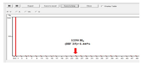
The submissions of Fourier had been of great value and had contributed to the analysis of the non-sinusoidal waveform by allowing any periodic function to be used or described in a series of sinusoidal and co-sinusoidal functions(Grady, 2012). For instance, if we are applying a fundamental frequency of 50Hz, then the second harmonics will be 100Hz, and the third, 150Hz, and so on. The respective harmonics can sum up to reproduce the original waveform and the highest harmonics of interest in power system is usually the twenty-fifth and this is in the low audible range (Soni and Soni, 2014)

Over twenty years now, there had been an appreciable and noticeable effort geared towards the analysis of power system harmonics. In this analysis, procedures for simulation methods and component models had been put in place such that the study of harmonics is becoming an important component of power system analysis and design (Durdhavale, 2016). Based on this and the knowledge of digital computers, computer simulation is now the preferred method to conduct harmonic analysis. Computer modeling for power systems for harmonic analysis and computer simulation of harmonic propagation in power systems are the two main aspects of harmonic analysis [7].

In theoretical terms, an ideal power system produces a perfect sinusoidal voltage signal at the load side but such theory is difficult to achieve practically. A distortion in power system is said to have occurred when there is a deviation from the perfect sinusoidal waveform. When this is experienced, then harmonic distortion has occurred. When electrical equipment is working in good and normal condition or when it is not loaded, only odd harmonics are produced but when transient conditions or possible equipment mal-function exist, then the system will generate even harmonics.

The present situation of poor power quality in industrial and commercials sites, especially harmonics had created some form of attention to one of the power problems in the world; harmonics. This situation is as a result of the growth in the use of non-linear loads. The increase in the use of non-linear load had brought about the tight recommendations of IEEE standard 519 especially in the industrial and commercial sector (Robert G.Ellis, 2011). Harmonics in power system should not be treated with levity as they are of great concern in the power sector. Harmonics usually affects power infrastructure and the equipment therein and most times causes a down time in operations as people may think that the problem at that point is load related. Harmonics in power system lead to situation of over-current and over-heating leaving an impression of a possible situation of overload in the power system.

2. Discussion

2.1 Fundamentals of Harmonics

Harmonics can also be known in power system as distorted waveforms and the classification of these waveforms fall in two categories; the voltage and current harmonics. There two concept also used to describe harmonics; they are the orders of harmonics and symmetrical components. Generally, harmonic component is illustrated in the equation below:

Where
f_n = current amplitude of nth order harmonic
f₁= fundamental current amplitude.

Figure 1: Decomposition example of a complex distorted signal, as addition of 50Hz

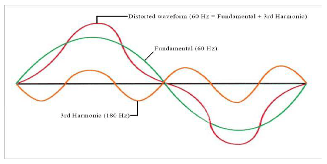
Fundamental and 3^rd , 5^th and 7^th harmonics (150Hz, 250Hz, 350Hz respectively) (Pinyol, 2015) There is harmonics in a power network if the component of a waveform occurs at an integer multiple of the fundamental frequency. In the description of harmonic orders, the odd order harmonics and the even order harmonics are the common nomenclatures known for classification. However, there is a third classification, the triplet harmonic which is not much known. The table 1 below shows the classification of harmonics in terms of the “order”. Presently, the characteristics of the harmonic component in the power system are the odd harmonics and the odd harmonics are also represented by the waveform that symmetrical to the time axis. Even harmonics are only produced from waveforms that are not symmetrical to the time axis (Durdhavale, 2016).

Table 1: Harmonics Order (Durdhavale, 2016)

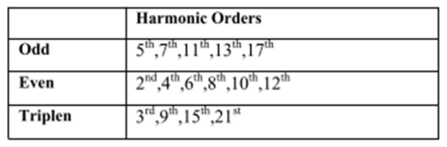
There are three broad categories in which harmonics can be placed and this is expressed in terms of sequence. The positive sequence harmonics, negative sequence harmonics and the zero sequence harmonics. The positive sequence harmonics are made up of the 4^th, 7^th, 10^th, 13^th and 19^th , ….3k+1 order harmonics and the negative sequence harmonics are consist of the 2^nd , 5^th, 8^th, 11^th, 14^th, and 17^th …2k+1 order harmonics while the 3^rd, 6^th 9^th , 12^th and 15^th, 3k+3 order harmonics are attributed to the zero sequence harmonics. Where k ranges from 0, 1,2,3, etc. See Table 2 below for illustration (Kamenka, 2014). In a system where three phase four wire is the wiring arrangement, the zero sequence harmonics system the zero sequence harmonics drifts through the neutral connection and causes an overheating of the conductor (Dash et al., 2014).

Table 2: Symmetrical Component of Harmonics (Kamenka, 2014)

Figure 2: Harmonic Distortion for a 50HZ Power System [11]

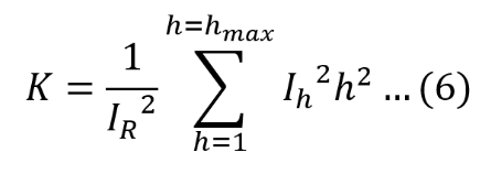
Fourier postulated a theory and in his theory, we were able to depict that any The Fourier theory tells us that any repetitive waveform is defined as the sum of the sinusoidal waveforms which are integer factor of the fundamental frequency. With the consideration of a steady state waveform with characteristics of equal positive and negative half cycles, the Fourier series can be expressed in equation 2 as shown below (Dash et al., 2014)

Where
f(t) = the time domain function.
n = the harmonic number (putting in consideration odd values only).
A_n = the amplitude of the nth harmonic component.
T = the period or length of one cycle in seconds.

It is worthy of note that harmonics being a steady state phenomenon will repeat every 50Hz or 60HZ cycle, depending on the power system in place. Spikes, dips and other forms of transient do not imply a situation of harmonics and should not be confused with harmonic condition (Robert G.Ellis, 2011).

2.2 Power Quality Indices under Harmonics

i. 2.2.1 Total Harmonic Distortion

The factor that is mostly used to determine the deviation of distorted waveforms from a sine wave is called Total Harmonics Distortion (THD) and this is described in relation with the degree of distortions in both the waveforms of the current and voltage in the power network. The calculation of distortion in the voltage and current is given in equation 3 below. As it may be seen in other publications or books, another term that can be used to describe the Total Harmonic Distortion is known as the Distortion Factor (DF) (Robert G.Ellis, 2011).

Where

ID_n represent the magnitude of the nth harmonic as a percentage of the fundamental (individual distortion). Grady, in 2012 [4] defined THD as the ratio of the root mean square value (rms) of the harmonic above fundamental to the rms value of the fundamental. Marcuello, Arcega, Plaza, & Ibáñez, in 2011[12] termed THD as the rms value as the proportion of of all harmonic components together to the rms amplitude of the fundamental harmonics. In a white paper by Eaton in 2017 (Eaton, 2017), THD was described as the fraction of the total power of all harmonic components to the power of the fundamental frequency. Similar definition was also given by Durdhavale, in 2016.

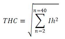
Total Harmonic Current (THC)

The summations of current orders 2 to 40 are the cause of distorted waveforms leading to Total Harmonic Current. The value of the Total Current Harmonics (THC) is basis for the installation of active filters. Mathematically, THC can be illustrated as in equation 4 (Durdhavale, 2016).

Where I_his the harmonic current of the nth order.

Total Harmonic Distortion Current (THDi)

The Total Harmonic Distortion Current (THDi) describes the magnitude of distortion present in a waveform It is derived from the fraction of the Total Harmonic Current (THC) and the fundamental current. It is expressed mathematically as shown in equation 5 below (Durdhavale, 2016)

Where I₁ is the fundamental current

Total Harmonic Distortion of Voltage (THDv)

This is a representation of the total value of the voltage distortion in a given waveform. It can be derived from the ratio of the harmonic voltage to the non-harmonic or fundamental voltage (Pinyol, 2015). THDv can be expressed as:

Where V_n = voltage amplitude of the nth order harmonic, V₁ = fundamental or non-harmonic voltage amplitude.

Total Demand Distortion (TDD)

Total Demand Distortion is commonly used to describe harmonics in the North America region. It is however defined as the division of the harmonic current by the full load fundamental current. The full load current is also the total non-harmonic current demanded by all load at peak time. Mathematically, it can be written as shown in equation 7 below.

Where I_n is termed as the current amplitude of the nth order harmonic, I_L is the total load current demand by the system.

The definitions of THD and TDD are alike only that THD compared the harmonic content with measured fundamental current while TDD evaluates its distortion with the maximum demand current. Considering the definitions of the fundamental current (I₁) and the maximum demand current (I_L), the value of I_L is greater than I₁ for harmonic measurement purpose, hence the value of TDD and the percent of I_L will tend to be lower than THD and its corresponding percent of I₁ measurement. The determination of the values of THD and TDD is relevant as it assist in determining the accurate value of harmonic generated by a facility’s power network during the time where light loads are being used. (IEEE Recommended Practices and Requirements for Harmonic Control in Electric Power Systems, 1992)

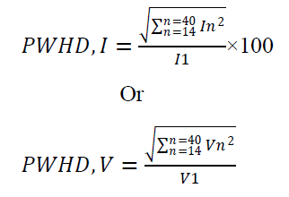
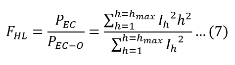
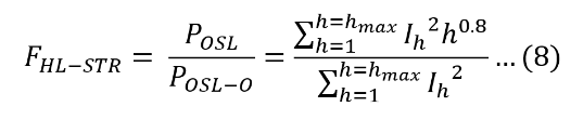
Partial Weighted Harmonic Distortion (PWHD)

PWHD can be expressed as the ratio of the voltage or current within a selected group of harmonics higher order (say 14^th order to 40^th order) to the fundamental values of the current or voltage, as the case may be. PWHD equations for current and voltage can be given as shown in equation 8 and 9 below (Durdhavale, 2016)

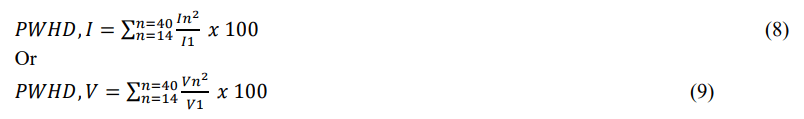
Where I₁ can be expressed as the fundamental current amplitude, and V₁, the fundamental voltage amplitude.

2.3 Sources and Causes of Harmonics Distortion

Harmonics come into play as a result of non-linear loads in the power network. In recent times, enhanced power semiconductor technology coupled with power electronics devices are now used in various applications in the field of electrical and electronics engineering. These applications are in the classification on non-linear loads and thus the devices demand current with harmonic content and reactive power from the AC component of the power network (Panda et al., 2013).

For better understanding of the sources and caused of harmonic distortion, it is important to explain briefly the term “non-linear load”. We can say that a load is non-linear when the current demand from such load does is not even with the connected sinusoidal voltage. This implies that the Ohm’s law is not applicable in describing the Voltage-Current relationship as the resistance is not a constant value any longer and there will be a change in current value with each produced sinewave of the applied voltage waveform. This situation causes several positive and negative pulses. The varying current values are termed to be non-linear and they produce frequency components that are manifolds of the frequency of the power system. Besides the fact that the non-linear current produces multiples of the frequency of the power system, they also form a network with the impedance of the electrical power supply to form voltage distortion that can affect the power network and the load on it (Kamenka, 2014).

The simplest network that can be used as an illustration for a non-linear load is a diode-rectifier in its various applications such as the half-wave diode rectification, full wave diode rectification in both single phase and three phase network (Pinyol, 2015). Table 3 below shows the various classification of non-linear load responsible for the generation of harmonic distortion in a power network.

Table 3: Non-Linear Loads (Kamenka, 2014)

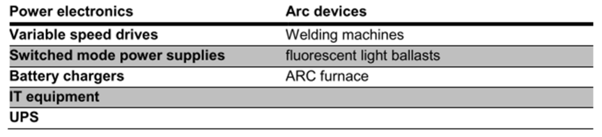
Prior to now, equipment with magnetic iron cores like electric motors, transformers and generators were known to be predominant in the cause of harmonic distortion in power network. Likewise, the arc furnaces and the arc welder’s equipment also cause harmonic distortion in power network. In recent times, where energy efficiency is crucial, there had been some introduction of power electronic equipment to enhance energy efficiency utilization and these equipment had contributed to the most serious source of harmonics within a power network in industrial and commercial facilities (Kamenka, 2014).

ii. 2.3.1 Transformers The magnetization curve explains the correlation between the input or primary voltage and current of a transformer. A transformer is working in normal condition does not generate any form of harmonic distortion unless the transformer is in a core saturation condition. At this condition, the harmonic distortion increases appreciably with the odd orders of harmonics, the third order being dominant. This kind of condition is show cased when the transformer is operating in an overload condition, especially during peak periods or when the transformer is subjected to an overvoltage condition, especially at situation of low power demand or possible switching of large reactive power load. This harmonic content is manifested in the magnetization curve of the transformer as in figure 3 below. When the transformer is working in normal condition, a little increase in the voltage usually result in a little rise in the magnetization current. Similarly, when an overvoltage condition exist, that is when the voltage is above the nominal voltage, then a small increase in voltage will result in having a large increase in the magnetization current (Kamenka, 2014).

Figure 3: Transformer Magnetization Curve (Kamenka, 2014)

iii. 2.3.2 Rotating Machines

Generators and Motors are examples of rotating machines and they also produce magnetizing field like transformer, hence they are capable of producing harmonics in power network. Though the harmonic content of produced as a result of the magnetization curve of motors is much more linear when compared to that produce by a transformer, thus, the harmonic content is not disturbing, however, the higher capacity motors have capacity of generating high harmonic content. On the other hand, generators produce observable voltage harmonics following the unpractical nature of the spatial distribution of the stator winding. The voltage harmonics produced from a generator are the 3^rd order harmonics which in turn causes creates a 3^rd order current harmonic in the power network (Durdhavale, 2016).

iv. 2.3.3 Arc Furnaces and Arc Welders

Arc furnaces and arc welders are high power consuming equipment that also produce corresponding high level of harmonic distortion in a power network. Arc furnaces are applicable in air refining, refining and melting applications and these phases produces different levels and gradients of harmonics. The random variation of the arc produces a combination of ignition delays and voltage changes and this situation creates some sort of harmonic spectrum with odd and even multiples of fundamental frequency. These frequencies changes intermittently with various swift levels of rise and falls (Suresh and Babu, 2015)

Figure 4: Harmonic Current Spectrum in Arc Furnace (Kamenka, 2014).

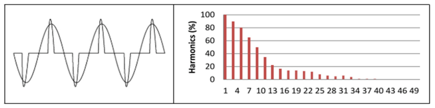
v. 2.3.4 Switched Mode Power Supplies (SMPS)

Most of the electronic devices of today are embedded with Switched Mode Power Supplies and the name is on the basis of the switching and conversion of unregulated DC input voltage to a regulated DC output voltage. Based on the SMPS principle of operation where rectifying and filtering at various stages is involved, this result in the demand of pulses of current instead of continuous current. This pulse is made of high content of harmonics of the third order and even higher orders. A typical waveform and the harmonic spectrum is shown in figure 5 below (Durdhavale, 2016)

Figure 5: Waveform and Harmonic Current Spectrum of SMPS (Kamenka, 2014)

vi. 2.3.5 Variable Frequency Drives

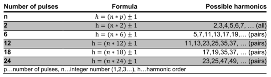
Variable frequency drives are applicable to equipment that uses the technology of static converters in a three-phase bridge system. We can term the bridge as six-pulse bridge or B6 bridge. This same technology is also applied in UPS application as well as inverter applications, basically AC to DC converters. The term B6 as earlier mentioned came to being from the trend of pulse generated, six voltage pulses per cycle which corresponds to the production of one pulse in a half cycle per phase. The harmonic spectrum in this case is attributed to the magnitude of pulses of the variable frequency drives. The current harmonics that emanates from a B6-bridge is in the 6n ± 1 orders which implies that we can either have orders in the form of 5^th and 7^th, 11^th and 13^th, 17^th and 19^th, just to mention a few. As the harmonic spectrum is dependent on the number of pulse, so the harmonic spectrum will be different if 12 or 18 pulse converter is applied for the application. See table for more information. Figures 6 illustrate how the waveform looks like; its resulting harmonic spectrum is also included.

Table 4: Pulse and Harmonic Spectra in a Variable Speed Drive (Kamenka, 2014)

Figure 6: Waveform and Harmonic Spectrum of a B-6 Variable Speed Drive (Kamenka, 2014)

2.4 Effects of Harmonics Distortion

Implications of harmonics within the power network can be categorized in terms of their duration, for instance, it could either be short term or long term. The failures or malfunctions of equipment or devices subjected to harmonic distortion can be categorized as short term effects while long terms effects can be linked with the thermal behavior of the devices or equipment. Harmonic situation lead to scenarios of thermal build-up or temperature rise in equipment and electrical network. When there are situations of increased temperature of electric or electronic devices, cables, motors arc, then besides the effect of higher losses, the equipment or system life becomes reduced (Suresh and Babu, 2015).

vii. 2.4.1 Power Factor

When there are situations of harmonic distortion in a power network, the power factor of the network gets affected following a higher demand in the level of current. The power factor becomes exceedingly low if there is an increase in the phase shift between the voltage and current, certainly with a situation of current harmonics within the system. Power factor can simply be explained in terms of the relationship between the active power and the apparent power. It can be defined as the ratio of the true power (in watts) to the apparent power (in VA). It determines or measures the efficiency of the energy used by a load in a power network. Power system with a high power factor demands less current when compared to that with a low power factor under the same power conditions. This implies that systems with higher power factor are more efficient than those of lower power factor. The effects of harmonic distortion which is predominant in non-linear load tend to cause a situation of bad power factor, thus lowering the efficiency of the system (Kamenka, 2014).

viii. 2.4.2 Phase and Neutral Conductors

Practically, three phase system are such that they possess phase angles and in an ideal system, the phase voltages are displaced by 1200 from one another. If the system is subjected to load and the individual phases are equally loaded, the resultant neutral current will be zero but if there is presence of current harmonic in the system, then the triplen harmonic will sum up in the neutral link so much that the total current in the neutral surpass the individual current in each of the phases, to a factor of three. This scenario may cause a situation of overload on the individual current and the neutral current. This can result in the overheating of the cables and the conductors may eventually get burnt (Kamenka, 2014).

ix. 2.4.3 Transformer

Transformers are devices that are widely known for the supply of electric power to facility loads which includes both linear and non-linear loads. Transformers are affected by harmonics in two specific ways; there are situations of additional losses within the transformer core and production of triplen harmonic current. The losses generated are a result of eddy current, resistive and magnetic losses in the core. These additional losses produce extra heat within the system which overtime reduces the operating life of the transformer insulation. For the purpose, especially in industrial applications with load that are non-linear, transformers cannot be put into use at full load because of the high level of harmonic distortion (Soni and Soni, 2014).

x. 2.4.4 Rotating Machine

Similar to the effect of harmonics on transformer, harmonics also result in additional power loss in motors and generators. The effect of the losses is such that there is high temperature build up within the devices as a result of the increase in the resistance of the system which is directly proportional to the rate of frequency increase. Hence, the harmonic current will lead to increased losses in the windings of the rotating machines. Another effect of harmonics on the rotating machine is the generation of higher vibrations inside the bearings and this can cause wear and tear within the system with an eventual earlier equipment weakness (Pinyol, 2015).

xi. 2.4.5 Circuit Breakers

Harmonic tend to cause an increase in current in power network and tend to create situations of incessant tripping in the system thereby disrupting operations. A residual current circuit breaker (RCCB) functions to sum up the current in the phase and neutral conductors and disconnects the power from load peradventure the summation does not fall within the rated limit. Harmonic situation disrupt this operation as the RCCB may not be able to add the high frequency component correctly leading to nuisance tripping that can result in shutdown in production process, loss of time and money (Ritesh Dash, Kunjan K. Mohapatra, Patrik R. Behera, 2014)

xii. 2.4.6 Power Factor Correction Capacitors (PFC)

The factors that lead to the dielectric breakdown of capacitors are temperature, voltage, current and overload in power. Situation of harmonics seriously have adverse effect on PFC capacitors such that an increase in the maximum value of voltage based on high harmonics creates additional dielectric stress, thereby causing partial discharge in the insulation and permanently damaging the capacitors. In most cases, issues that relate with capacitor performance or behavior are related to current. Also, the impedance with respect to the voltage harmonics decreases as the harmonic order increases because the relationship of the capacitive reactance to the frequency is not linear. Therefore, capacitors with voltage harmonics absorb higher current when compared with capacitors in a system without voltage harmonics. In essence, this implies that voltage harmonics in a system give rise to a situation of high current draw in capacitors and causes additional losses, quick aging of the insulation and the eventual damage of the PFC. This effects are aggravated if the harmonics are multiples of parallel or series resonance (Ciurro, 2009)

xiii. 2.4.7 Lights

Incandescent lamps are generally non-linear loads and the useful life or age decreases with the level of harmonics present. Lamps with features comprising of ballast inductor or capacitor do present a resonance problem which causes harmonic distortion; thus if the lamp is operated at about 105% of its rated voltage, then its useful life falls by an approximate value of 47% (Suresh and Babu, 2015).

2.5 Harmonics Mitigation Techniques

In line with the sources and causes of harmonic distortion in power system, various elimination or mitigation techniques to trap or limit the occurrence of harmonics with different levels of effectiveness and efficiency are considered below.

1. Introduction of Active Harmonic Filter The use of active harmonic filters in a power system introduces current component that can negate the effect of the harmonic contents in a non-linear load. Active harmonic filters come in different forms such as the series filter, shunt filter and hybrid filter but the most recent technology of harmonic filter available is the active filter. Active filtering technique is applicable in standalone applications or by installing the design in the input stage of a drive, UPS system or other power electronic devices. Considering all technologies in UPS application except from the use of Insulated Gate Bipolar Transistor (IGBT), the harmonics generated in these system are greater than the expected for most electrical system; hence the need for the input filter to reduce the harmonic content to a value which is less than 10 percent of total harmonic distortion of the input current. The addition of a transformer in the system will produce more inductance to the line which will additionally lower the harmonic distortion in the system (Steele, 2015).

Ideally, the active filter operates in such a manner that it observes the load current and eliminates the fundamental frequency current after which it will investigate remaining frequency content and the respective magnitude. Based on this analysis, the active filter will be able to pass in the required equal and opposite current to eliminate the different harmonics. The active filter has the capacity to cancel harmonics to the 50th order and achieve a low level of current harmonic distortion to a value as low as 5%. In order to use active harmonic filter in the power network, there is the need to take a measurement of the harmonics to be cancelled from the system after which an active filter that possesses the magnitude of harmonic current required to cancel the measured harmonic can be selected (Soni and Soni, 2014)

2. Use of K-Rated Transformers In Power Distribution Components

Generally, transformers are not manufactured and designed to operate under high harmonic content produced from the presence of non-linear load in the power network. The effect of this harmonics is such that it raises the magnetization core of the device leading to overheating and eventual sudden failure when in use. The introduction of harmonics into power system brought about the development of the K-rated transformers. K-rated transformers are not design to eliminate harmonic, rather they are designed to handle the generated heat from the harmonic current. K- Factor values are within the range of 1 to 50 whereas a standard transformer that supplies linear load has a K-factor of 1. A high value of transformer’s K-factor implies that the transformer can handle higher the degree of thermal energy generated from the harmonic current. The choice of transformer in terms of the K-factor is important in installation design and this is also dependent on the magnitude of harmonic content in the power network. Table 5 below shows the K-factor ratings that are applicable for different percentage of harmonics (Eaton, 2017).

Table 5: K Factors Rating for Different Non-linear Load in Electrical System (Eaton, 2017)

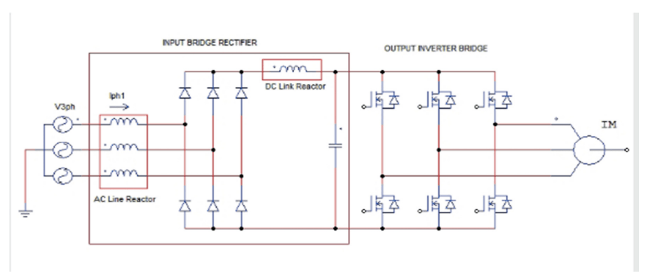
3. Introduction of Line Reactors

In order to control the harmonic distortion produced in a Variable Speed Drive (VFD), there is the need to connect a series reactor with non-linear load at the input line of the drive (Ritesh Dash, Kunjan K. Mohapatra, Patrik R. Behera, 2014)

A line reactor, also called input AC reactors can simply be explained as an inductor that is connected in series between a load and the source. . It functions to limit the current the current harmonic characteristic thus reducing harmonic in the system (Rockwell and Wisconsin, 2016).

A line reactor also helps to mitigate the harmonics which the VFD creates back into the line. The rating of line reactor is in horse-power (hp) and the voltage rating of the drive is applicable for use. The figure below is an illustration of a VFD circuit of motors showing the AC and DC reactors. (Lenz, 2008)

Figure 7: Circuit of a VFD of Motors Indicating the AC and DC Line reactors (Pinyol, 2015)

4. Over-sizing or Derating of the Installation

In reducing the effect of harmonics in a power system, the solution that is mostly implemented by technical personnel is to dimension for an oversized neutral conductor. However, where there is an existing installation, the solution is to reduce the capacity of the electrical distribution equipment experiencing the harmonic distortion. In modern times, the dimension of the neutral wire is always rated in the same size as the individual phase wires and may even be dimensioned (Soni and Soni, 2014).

2.6 Recommended Harmonic Limit – IEEE Std. 519™-2014

Both the end users and power system operators should be responsible for the management of harmonics in power network. Harmonic limits recommendation span through the voltage and current parameters in a power network and the recommended values are on the premises that some level of voltage distortion are generally acceptable and it is the responsibilities of all parties involved to ensure that the actual voltage distortion is kept below the generally accepted limits. The basis of this recommended limit is that in the act of limiting the harmonic current in a system, and then voltage distortion can be within the recommended level (Committee, Power and Society, 2014).

The application of the recommended limit is applicable only at the point of common coupling and cannot be used in the applications of either individual equipment or locations in the industry or facilities. The various recommended limits for voltage and current harmonics are as shown in the following tables below.

Table 6: Recommended Voltage Distortion Limit (Committee, Power and Society, 2014)

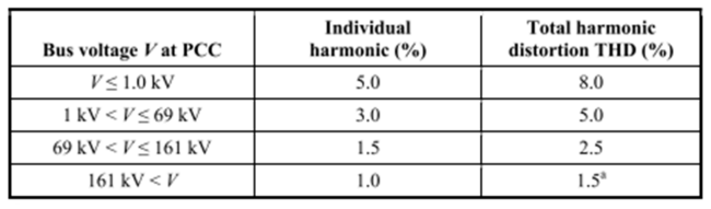
Table 7: Recommended Current Distortion Limits for Systems rated 120V through 69kV (Committee, Power and Society, 2014)

Table 8: Recommended Current Distortion Limits for Systems rated 69kV through 161kV (Committee, Power and Society, 2014)

Table 9: Recommended Current Distortion Limits for Systems rated >161kV(Committee, Power and Society, 2014)

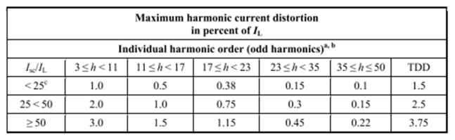
Based on the indices on Table 6 to 9, the following are defined as:
a= Even harmonics are limited to 25% of the odd harmonic limits above.
b= Current distortions that result in a dc offset, e.g., half-wave converters, are not allowed.
c= All power generation equipment is limited to these values of current distortion, regardless of actual I_sc/I_L.

Where I_sc relates to the peak short-circuit current at PCC, I_L is defined as the peak demand load current (fundamental frequency component) at the PCC under normal load operating conditions.

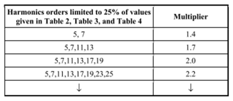
2.6.1 Recommendations for Increasing Harmonic Current Limits

Following recommendations, the values as seen in Table 7, Table 8 and Table 9 can be increased by a multiplying factor when the user decides to reduce the magnitude of lower-order harmonics. The multipliers are given in Table 10 below and are put into use when steps are taken by the user to reduce the harmonic order shown in the first column of the table.

Table 10: Recommended Multipliers for Increasing the Harmonic Current Limit (Committee, Power and Society, 2014).

3. Conclusion

This paper presented research on harmonic distortion in the voltage and current waveform with respect to the existing level of harmonic distortion in the power system at the moment and the possible look at how harmonic will be portrayed in future.

Harmonics in power system is caused by the presence of non-linear load within the network. The different categories of equipment that give rise to harmonic distortion have numerous harmonic spectra and the peculiar harmonic spectra related to particular type of load can only be determined by having the requisite knowledge and experience in harmonics. Most of the harmonics generated from non-linear load are predominant in the electronics components which form the basis of modern technology. The demand for these types of equipment may result in serious problem in the future and the harmonic generated from these systems will significantly affect the power quality.

Harmonics in power system should not be treated with levity as they are of great concern in the power sector. Harmonics usually affects power infrastructure and the equipment therein and most times causes a down time in operations as people may think that the problem at that point is load related. Harmonics in power system lead to situation of over-current and over-heating leaving an impression of a possible situation of overload in the power system.

The problem of poor power quality relating to harmonics is not often noted by most practicing electrical engineers and consulting engineering firms and such problems if not critically analyzed would have impeded operations and establishment would have incurred a high cost in finding a solution; with an eventual damage to equipment. Good understanding of the causes, potential effects and means of mitigation can assist in the reduction of harmonic in the power system especially in the design stage of power infrastructure and the probabilities of undesired effect occurring can be reduced.

Acknowledgement – I am grateful to the school of Science and Engineering at Atlantic International University, Honolulu for giving me the required platform to be able to complete the research and analysis of this paper. I also acknowledge my team members at Powerex Limited for their understanding and cooperation while carrying out this research paper.

Profound gratitude goes to my wife and children; Ogunyemi Moyofoluwa, Oluwatofunmi and Oluwatoni for their support and understanding towards theh completion of this paper. You are greatly acknowledged.

References

Abdelaziz, A. Y., Mekhamer, S. F. and Ismael, S. M. (2012) ‘Sources and Mitigation of Harmonics in Industrial Electrical Power Systems : State of the Art’, (October).
Ciurro, N. (2009) ‘Harmonics in Industrial Power Systems’, (June).
Committee, D., Power, I. and Society, E. (2014) ‘IEEE Recommended Practice and Requirements for Harmonic Control in Electric Power Systems IEEE Power and Energy Society’, 2014.
Dash, R. et al. (2014) ‘FUNDAMENTALS OF HARMONICS AND ITS EFFECT ON’, 3(4), pp. 790–794.
Durdhavale, S. R. (2016) ‘A Review of Harmonics Detection and Measurement in Power System’, 143(10), pp. 8–11. Eaton (2017) ‘Harmonics In Your Electrical System’, What they are, how they can be harmful, and what to do about them, pp. 1–7. doi: 10.1164/ajrccm-conference.2017.A35.
Grady, P. M. (2012) ‘Understanding Power System Harmonics’, Chapter 1, (April).
IEEE Recommended Practices and Requirements for Harmonic Control in Electric Power Systems (1992) ‘IEEE std 519-1992’, Ieee, pp. 1–9. doi: 10.1109/PAPCON.2006.1673767.
Kamenka, A. (2014) ‘Six tough topics about harmonic distortion and Power Quality indices in electric power systems A white paper of the Schaffner Group Written by Alexander Kamenka’. Lenz (2008) ‘Application Note- When to Use a Line or Load reactor’, (July), pp. 1–3.
Marcuello, J. J. et al. (2011) ‘A Review of Teaching Power System Harmonics’, 1(2), pp. 1–5.
Ogheneovo Johnson, D. (2016) ‘Issues of Power Quality in Electrical Systems’, International Journal of Energy and Power Engineering, 5(4), p. 148. doi: 10.11648/j.ijepe.20160504.12.
Panda, G. et al. (2013) ‘Novel schemes used for estimation of power system harmonics and their elimination in a three-phase distribution system’, International Journal of Electrical Power and Energy Systems. Elsevier Ltd, 53, pp. 842–856. doi: 10.1016/j.ijepes.2013.05.037.
Pinyol, B. R. (2015) ‘HARMONICS : CAUSES , EFFECTS AND MINIMIZATION’, (August), pp. 1–32.
Ritesh Dash, Kunjan K. Mohapatra, Patrik R. Behera, M. R. S. (2014) ‘A REVIEW ON POWER SYSTEM
HARMONICS School of Electrical Engineering , Kiit University’, Indian Journal of Research, pp. 1991–
1992.
Robert G.Ellis, P. E. (2011) ‘POWER SYSTEM HARMONICS A Reference Guide to Causes ’, pp. 1–3.
Rockwell, A. J. T. S. and Wisconsin, M. (2016) ‘Line Reactors and AC Drives .’
Soni, M. K. and Soni, N. (2014) ‘Review of Causes and Effect of Harmonics on Power System’, 3(2), pp. 214– 220.
Steele, B. J. (2015) ‘Mitigate damaging harmonics’, (August), pp. 39–41.
Suresh, N. and Babu, R. S. R. (2015) ‘Review on Harmonics and its Eliminating Strategies in Power System’, 8(July). doi: 10.17485/ijst/2015/v8i13/56641.

Source & Publisher Item Identifier: Journal of Energy Technologies and Policy http://www.iiste.org ISSN 2224-3232 (Paper) ISSN 2225-0573 (Online) Vol.9, No.3, 2019. Publication date: March 31st 2019. DOI: 10.7176/JETP/9-3-02, https://core.ac.uk/download/pdf/234668516.pdf.

A Review of Harmonics Detection and Measurement in Power System

Published by 1. Dnyaneshwar D. Ahire, Professor, Matoshri College of Engineering and Research Centre, Nashik Savitribai Phule Pune University, Nashik, Maharashtra, India.
2. Snehal R. Durdhavale Student, Matoshri College of Engineering and Research Centre, Nashik Savitribai Phule Pune University, Nashik, Maharashtra, India.

ABSTRACT – A load is said to be “linear” when it draws a current from the supply which is proportional to the applied voltage (linear). And in the case of “non-linear” load, impedance changes with applied voltage. The current drawn from such non-linear load is also non-linear i.e. non-sinusoidal even when it is connected to a sinusoidal voltage source. Harmonic currents contents which are present in non-sinusoidal currents intermingle with the impedance of the power distribution system to create voltage distortion which affects the distribution system and the loads connected to it. The serious power-line pollution is a result of increasing use of power electronic systems and time-variant nonlinear loads in industry. Hence, power supply quality is degraded. It results in the reduction of system efficiency, apparatus overheating, and increase power. As the utilization of the number of harmonics-producing loads has increased over the years, it has become highly mandatory their influence and analysis when making any additions or changes to an installation. In this paper various harmonics detection and measurement techniques have been outlined.

Keywords: Non-linear loads, harmonic currents, power distribution system, voltage distortion, power signal quality, harmonic distortion.

1. INTRODUCTION

Power quality can be defined as a set of electrical boundaries allowing an equipment to function in its intended manner with no significant loss of performance or life expectancy. Various methodologies and techniques were proposed to improve the power quality. A power system ideal when is define when a perfect sinusoidal voltage signal is seen at load-ends. Practically, such idealism is really hard to maintain. Any deviation from the perfect sinusoidal waveform is nothing but distortion and hence harmonic distortion. It has been said about harmonics is they are voltages or currents with frequencies which are integer multiples of the fundamental power frequency. Only odd harmonics will be produced by electrical equipment’s, when working in normal or no load condition. When transient conditions or conditions of mal-function or single-phase rectification appear, even harmonics may occur. One of the parameters which affect the quality of power is harmonics current are supplied by the non-linear equipment, which disrupts the desired linear system. These distorted current pulses, due to Ohm’s law, will also instigate to distort the voltage waveforms, where these distortions would be carried back to the distribution network. Common risks of harmonics include potential fire hazard, excessive heat, false tripping of branch circuit breakers and consequently increases maintenance cost [2], [3].

1.1 Basics

In any power system, it is highly impossible to accomplish a perfect or pure sinusoidal waveform at every point of a network. The voltage and current waveform deviate massively from a sinusoidal waveform. These waveform deviations are usually called harmonic distortion.

“Harmonics” is the term which means waves having frequencies of integer multiples of one another. The harmonic component in an AC power system is nothing but the sinusoidal component of a periodic waveform that has a frequency of an integer multiple of the fundamental frequency of the system. It can be given as:

f_h= n*fundamental frequency

Where, f_h= harmonic order, n= integer, and the fundamental frequency is either 50Hz or 60Hz.

For example, if a system has the fundamental frequency as 60Hz then its 2^nd and 3^rdharmonic would have frequencies of 120Hz and 180Hz respectively[1],[[2].

Figure 1: Harmonic distortion of the electrical current waveform [2]

1.2 Classification of Harmonics

Harmonics which are nothing but distorted waveforms have two types namely voltage and current harmonics. The orders of harmonics and symmetrical components these are two concepts which are used commonly to describe harmonics. Regarding the harmonics, words odd and even harmonics are used usually but the term triplen harmonics is not much known. Table shows harmonic orders:

Table 1. Harmonic Orders

In the present scenario, odd harmonics are the characteristics harmonic components in the power network. Waveforms that are symmetrical to the time axis are represented by odd harmonics. In the case of even harmonics, they can only arise from waveforms that are not symmetrical to time axis [16].

1.3 Power Quality Indices under Harmonic Distortion

[16] Generally, representation of harmonic components is given with equation:

Where 𝑓𝑛= current amplitude of nth order harmonic, 𝑓1=fundamental current amplitude.

1.3.1 Total Harmonic Distortion (THD)

This notification is used widely in defining the harmonic content level. It is given as the ratio of the power of all harmonic components to the power of fundamental frequency.

1.3.2 Total Harmonic Current (THC)

Usually, distorted current waveform is caused by the contribution of current orders 2 to 40. THC value is used for installation of active filters. It can be written as:

1.3.3 Total Harmonic Distortion Current (THDi)

This value gives the total harmonic distortion of the waveform. This value can be calculated by taking the ratio of THC to the Fundamental current. It can be given as:

Where 𝐼1= fundamental current

Where 𝑉𝑛= voltage amplitude of nth order harmonic, 𝑣1=fundamental voltage amplitude. For the sake of good voltage quality, its value should be low.

1.3.4 Total Harmonic Distortion of Voltage (THDv)

It shows the total magnitude of the distortion in voltage. It can be calculated by calculating ratio of distorted or harmonic voltage to the non-harmonic or fundamental voltage. It can be written as:

1.3.5 Total Demand Distortion (TDD)

This concept is used widely used in North America regarding harmonics. It is the ratio of harmonic current to the full load fundamental current. The full load current is nothing but the total non-harmonic current consumed by all loads by the system when the system is on its peak demand.

Where 𝐼𝑛= current amplitude of nth order harmonic, Il= total load current consumed by system

1.3.6 Partial Weighted Harmonic Distortion (PWHD)

PWHD is the ratio of current or voltage with selected group of higher order harmonics from 14 to 40 to the fundamental value of voltage or current. PWHD for current and voltage can be given as:

Where, 𝐼1= fundamental current amplitude, V1= fundamental voltage amplitude.

1.4 Sources of harmonic Distortion

There are many harmonics sources are present but out of them few are listed here which play a role as the major sources of harmonics [14],[16].

1.4.1 Static Compensators

If the power source is fluctuating, static compensators are used at the ends of transmission lines or near sources of fluctuating power, static compensators manage the voltage. Reactors which are controlled by Thyristor will produce near about 1% of the 11th harmonic current.

1.4.2 Power Converters

Rectifiers give higher inductance on the dc side compared to the ac side. Hence the dc current is almost constant and then converter starts acting as a harmonic voltage source on the dc side where as the harmonics current source on the ac side.

1.4.3 Transformer

Because of saturation and hysteresis characteristics, a small level of harmonic current will get produce by transformers when they are in steady state. Initially high level of harmonics will be produced, which is 60% of the rated transformer current.

1.4.4 Rotating Machines

In the rotating machines, harmonic currents can be produced due to asymmetries in the winding pattern. Harmonics grow because of the resultant magneto motive force in the machine. Due to magnetic core saturation harmonic currents are generated.

1.4.5 Electric Arc Furnace

As the arc feed material varies, the harmonics rise up and their value cannot be predicted certainly. The electric arc furnace load gives most awful distortions a result of melting with the moving electrode and molten material.

1.4.6 Switched Mode Power Supplies (SMPS)

Latest electronic devices contain switched mode power supplies. SMPS regulates AC or DC input voltage. SMPS unit draws current pulses contain large amount of harmonics of third and above higher order harmonics.

1.5 Effects of Harmonics

Harmonics affect the power equipment’s and components. Following effects are shown on different components [14], [16]:

1.5.1 Power Factor

Harmonic distortion affects the power factor. Power factor gets worse with increasing amount of harmonic distortion. Generally, non-linear loads result in poor power factor.

1.5.2 Electric and Electronic Equipments

Basically, these equipments are considered as a source of harmonics. These devices are sensitive to harmonic distortion. They show effects as increase in supply voltage, zero crossing noise, malfunction of protective devices etc.

1.5.3 Conductors

On a regular basis, heat will be generated in the current carrying conductors due to I2R losses. As the harmonic orders increase, skin effect is produced. As the skin effect increases more I2R losses cause over heating of the conductors. Heating of conductors may also occur because of the magnetic field of harmonic currents in the neighboring conductors.

1.5.4 Transformers

Frequency causes Eddy current losses. Hence, as the harmonic order increases eddy current losses for transformers also increase. In addition to the skin effect, eddy current losses in transformer fallout in overheating and the life of the transformer would be reduced.

1.5.5 Capacitance

The Capacitors improve the power factor. They have a significant influence on harmonic levels. As the frequency of harmonics increases, the capacitive reactance decreases. As increased flow of current increase, the capacitor may get congested and impose higher dielectric stress.

1.5.6 Circuit Breakers and Fuses

Low level faults in circuit breakers caused because of the high degree of harmonic load current. High 𝒅𝒊/𝒅𝒕 ratings at zero crossings for sinusoidal waveform make the disruption complex, for load distortion. Hence, harmonic load currents results in circuit failures.

1.5.7 Lights

The distorted power supply decreases the life of the lamp gets decreased with. Harmonic currents give problems to audible noise in the case of discharging of lamps. In equipped with capacitors, together with the ballast inductor and the lamp may form a resonance problem.

1.5.8 Rotating Machines

Operating frequency plays a vital role in losses produced in the electric machines. Core and stray losses become significant for induction motor for an inverter producing high harmonic frequencies. The increase in temperature in the windings causes the lessening of life of the rotating machines. Communication between the air gap flux density and the fluxes generated by the harmonic currents in the rotor, pulsating torques are produced. By reason of the difference between time harmonic frequencies audible noises are formed. Additional problems in rotating machines caused by harmonics are equipment failure, bearing wear out, etc.

1.5.9 Telephone Interferences

Fundamental frequency doesn’t cause any serious problems but power system harmonics can cause huge problems because human audible sensitivity and telephone response peak have near 1 KHz. Inductive, capacitive and conductive interferences can be occurred between telephone line and a power line.

1.6 Why Harmonics should get detected?

Basically, harmonics are difficult to reduce. But the power quality gets reduced because of harmonics. They show economic impacts such as earlier failure of equipments, losses in distribution systems. So, they should be detected at early stage.

2. LITERATURE REVIEW

Tremendous work has been done for harmonics, their analysis and various mitigation techniques of harmonics. A brief review on this: For the reliable and efficient operation of any system a properly designed electrical system is necessary. And the system should be harmonic free.

For this purpose, capacitors in harmonic environment are applied. They are beneficial because they result in minimized THD, improved power factor and elimination of power factor penalties [3]. Lucian Asiminoae, Sergej Kalaschnikow and Steffan Hansen have discussed two harmonic detection methods. The methods are selective harmonic compensation and overall harmonic compensation [4].

An innovative method is presented for measurement of individual harmonics of a time-varying frequency. This proposed method is based on a nonlinear, adaptive mechanism. This technique offers the higher degree of accuracy, frequency-adaptivity [5]. David M. McNamara, Alireza K. Ziarani presented a new method of measurement of harmonics of time-varying frequency. This proposed method is based on the adaptive evaluation of the fundamental frequency and its harmonic components of the power signal [6].

A system made from a combination of the ARM9 chip and virtual instrument technology is designed for a real-time harmonic measurement. This system is presented in the paper [7].Frequency is a significant factor for harmonics measurement. The paper contains a review of several commonly used methods for power system harmonics measurement. And those methods are compared according to the aspect of frequency identification [8]. This paper gives a new idea for harmonic detection adopting the algorithm with combination of FFT with and wavelet transform. This instrument can obtain parameters of harmonic [9]. Hsiung Cheng Lin developed a strategy of recursive group-harmonic power minimizing for system harmonic and interharmonic evaluation in power systems. The proposed algorithm can measure integer harmonic and the interharmonics also identified accurately [10].

Harmonic components and harmonic distortion can be calculated using distortion meter. This paper presents the harmonic distortion meter based on microcontroller and its software part carries out calculations using DFT. DFT is used to find amplitude in order to measure THD in power system [11]. In this review paper an author has discussed abundant for selective harmonic detection methods in frequency domain as well as in time domain like DFT, FFT, SOGI technique and CDSP-PLL systems [12]. To estimate the fundamental frequency and to measure both harmonics and inter harmonics of any unknown frequency is not an easy task. But using the adaptive notch filter this can be done. This methodology measures fundamental frequency and harmonic and inter harmonic components fast [13].

Usage of non-linear loads in power system results in poor power quality. These loads are leading to harmonic sources; and this has become much serious problem. One of the widely used algorithms for harmonic analysis is Fast Fourier Transform (FFT). In this project, a harmonic analyzer is implemented using FFT on ARM7 core processor (LPC2138). For matching power rating the supply voltage is divided to 6V using the voltage divider. This harmonic analyzer can analyze harmonics in single phase supply and gives frequency spectrum of harmonics. This system has the advantage of being available in at low cost [15].

A constant wave Terahertz spectrometer is integrated with 1X2 LiNbO3 which is fiber coupled and customized optical phase modulator which allows direct modulation of Terahertz (THz) beam and measurement of the 1st and 2nd harmonics of modulation. Thus, using optical phase modulation rather than bias modulation harmonics measurement is carried out [17].

We know that harmonics is a very basic property of power quality. So it has become necessary a thing to measure these harmonics. Instead of using traditional measurement device a new method to detect and measure harmonics is presented. This device consists of the analog to digital converter, FFT unit, LCD display unit, and network communication unit. This methodology adopts FPGA and DSP processor. Experimental results show that using presented device more accuracy is obtained and harmonic power flow is also analyzed [18].

3. PROPOSED WORK

The various harmonic mitigation strategies adopted in the last three decades have been reviewed. Based on this survey a new methodology to control harmonic distortion in power system is introduced. In the proposed method harmonics get detected using ARM7 core processor (LPC2478). The software side performs FFT calculations for getting the amplitude of the fundamental frequency and the nth order harmonic. The distortion is calculated using the ratio of the amplitude of measured harmonic to the fundamental frequency.

The benefits of the proposed optimization method are:

1. Detection of harmonics in easier way
2.Correct measurement of harmonics and THD

4. CONCLUSIONS

Non-linear loads result in harmonic distortions in the power system and the associated problems were discussed briefly. Comprehensive review related to various methodologies to detect and measure harmonics in power system that was mentioned in the literature is done. Based on this review a new hybrid optimistic method to detect and measure harmonics is introduced in this paper. The system is designed for detection and measurement of harmonics on ARM 7 platform. Proposed system uses FFT algorithm for measuring total harmonic distortion.

5. REFERENCES

[1] Harmonics Detection and Filtering, Low Voltage Expert Guides by Schneider Electric.
[2] Harmonics in Your Electric System, A White Paper of Eaton Corporation.
[3] Douglas Andrews, Martin T. Bishop, John F. Witte,(May-June 1996), Harmonic Measurements, Analysis, and Power Factor Correction in a Modern Steel Manufacturing Facility, IEEE Transactions on Industry Applications, Vol. 32, No. 3.
[4] Lucian As iminoae,, Sergej Kalaschnikow and Steffan Hansen, Two harmonic detection methods used in industrial shunt active filters
[5] Masoud Karimi-Ghartemani, and M. Reza Iravani,( January 2005), Measurement of Harmonics/Inter-harmonics of Time-Varying Frequencies, IEEE Transactions On Power Delivery, Vol. 20, No.3.
[6] David M. McNamara, Alireza K. Ziarani, Thomas H. Ortmeyer(January 2007), A New Technique of Measurement of Nonstationary Harmonics, IEEE Transactions On Power Delivery, Vol. 22, No.1
[7] Weicheng XIE, Xia YANG, (2010), A Power Harmonic Measurement System Based on Wavelet Packet Transform and ARM9, IEEE.
[8] Gary W. Chang, Senior Member, IEEE and Cheng-I Chen, (2010), Measurement Techniques for Stationary and Time-Varying Harmonics, IEEE
[9] Shouxi Zhu, Wenlai Ma, (2012), Design of Power Harmonic Detection Instrument Based on DSP and ARM, CISME Vol.2 No.2
[10] Hsiung Cheng Lin, (February 2012),Power Harmonics and Interharmonics Measurement Using Recursive Group-Harmonic Power Minimizing Algorithm, IEEE Transactions On Industrial Electronics, Vol. 59, No.2
[11] Jaipreet Kaur Bhatti, Deepak Asati, (June 2012), Harmonic Detection using Microcontroller, International Journal of Computer Technology and Electronics Engineering (IJCTEE) Volume 2, Issue 3.
[12] Yi Fei Wang,Yun Wei Li,(2013), An Overview of Grid Fundamental and Harmonic Components Detection Techniques, IEEE
[13] Zhaobi CHU, Ming DING, Shaowu DU, Xueping DONG, (2013), Normalized estimation of fundamental frequency And measurement of harmonics/interharmonics.
[14] Alexander Kamenka, (2014) Six Tough Topics about Harmonics Distortion and Power Quality Indices in Electric Power System, A White Paper of Schaffner Group.
[15] Jeena Joy, Amalraj P.M., Aswin Raghunath, Nidheesh M.N Vinu Joseph,(August 2014), Harmonic Analysis of 230 V AC Power Supply Using LPC2138 Microcontroller, Transactions on Engineering and Sciences ,Vol.2, Issue 8.
[16] Manish Kumar Soni, Nisheet Soni, (February 2014), Review of Causes and Effect of Harmonics on Power System , International Journal of Science, Engineering and Technology Research (IJSETR), Volume 3, Issue 2.
[17] J. R. Demers, B. Kasper1, D.R. Daughton, (2015), Simultaneous measurement of the 1st and 2nd harmonics of a phase modulated coherent frequency-domain THz spectrometer
[18] Feng Guihong, Zhang Jing, Zhao Yisong , Ying Yong, Zhang Bingyil, Harmonic Power Detection and Measurement Device Based on Harmonic Power Flow Analysis.

Source & Publisher Item Identifier: https://ijcaonline.org/archives/volume143/number10/durdhavale-2016-ijca-910394.pdf , International Journal of Computer Applications (0975 – 8887) Volume 143 – No.10, June 2016.

Assessment of Flange Diffuser Structures to Improve the Power Generation of a Diffuser Augmented Wind Turbine

Published by 1. Yiyin KLISTAFANI, 2. A. M. Shiddiq YUNUS, 3. Muhammad ANSHAR, 4. Sri SUWASTI, State Polytechnic of Ujung Pandang, Indonesia (1) ORCID: 1. 0000-0003-3064-9612; 2. 0000-0002-9599-6941; 3. 0000-0001-5687-5023; 4. 0000-0002-7070-9651

Abstract. Wind energy has become the most popular renewable based power plant for the last decades due to its environment benighted and large natural availability. Although modern wind turbine successfully installed worldwide, some areas with low speed wind characteristic might require a special innovation to increase the amount of conversion of extracted wind energy into electric power. One of among popular techniques for the low speed wind turbine is Diffuser Augmented Wind Turbine (DAWT) which are continued to develop from time to time for example by using numerical simulation as an early stages before manufacturing. In this paper a numerical simulations are performed to investigate the effect of attached flange on wind velocity characteristics. Numerical simulations were carried out for the flow field around various flange diffuser type structures to improve the performance of a DAWT. The present studies specifically investigate the effect of attached flange to outlet diffuser with various flange’s angle (0°, 10°, 20°, 30°) on the wind velocity characteristics. Numerical studies were conducted using the Computational Fluid Dynamics (CFD) method. The studies demonstrate that the curved diffuser with flange 10° generates the strongest increment of the wind velocity compared to the other configurations. The maximum velocity inside the diffuser increases up to 115.14%. It is found that the wind velocity at the diffuser centreline is not capable to represent the overall velocity of each section. The curved diffuser with flange 10° shows the highest increment of the average wind velocity along diffuser with the greatest increment of 102.4 % at x/L = 0.36, and the highest increment wind velocity at the diffuser centreline section at x/L = 0.18 is 115.14%.

Streszczenie. Energia wiatrowa stała się najpopularniejszą elektrownią wykorzystującą odnawialne źródła energii w ciągu ostatnich dziesięcioleci ze względu na zaciemnione środowisko i dużą naturalną dostępność. Chociaż nowoczesne turbiny wiatrowe są z powodzeniem instalowane na całym świecie, niektóre obszary o niskiej prędkości wiatru mogą wymagać specjalnej innowacji w celu zwiększenia ilości konwersji wydobytej energii wiatru na energię elektryczną. Jedną z popularnych technik dla turbin wiatrowych o niskiej prędkości jest turbina wiatrowa z dyfuzorem (DAWT), która jest od czasu do czasu rozwijana, na przykład przy użyciu symulacji numerycznej jako wczesnych etapów przed produkcją. W artykule przeprowadzono symulacje numeryczne w celu zbadania wpływu przymocowanego kołnierza na charakterystykę prędkości wiatru. Przeprowadzono symulacje numeryczne pola przepływu wokół różnych konstrukcji typu kołnierzowego dyfuzora, aby poprawić wydajność DAWT. Obecne badania w szczególności badają wpływ zamocowania kołnierza do dyfuzora wylotowego o różnym kącie kołnierza (0°, 10°, 20°, 30°) na charakterystykę prędkości wiatru. Badania numeryczne przeprowadzono metodą obliczeniowej dynamiki płynów (CFD). Z przeprowadzonych badań wynika, że zakrzywiony dyfuzor z kołnierzem 10° generuje najsilniejszy przyrost prędkości wiatru w porównaniu z innymi konfiguracjami. Maksymalna prędkość wewnątrz dyfuzora wzrasta do 115,14%. Stwierdzono, że prędkość wiatru w osi dyfuzora nie jest w stanie przedstawić całkowitej prędkości każdej sekcji. Zakrzywiony dyfuzor z kołnierzem 10° wykazuje największy przyrost średniej prędkości wiatru wzdłuż dyfuzora z największym przyrostem 102,4% przy x/L = 0,36, a największy przyrost prędkości wiatru w środkowej części nawiewnika przy x/L = 0,18 to 115,14%. (Ocena konstrukcji dyfuzorów kołnierzowych w celu poprawy wytwarzania energii w turbinie wiatrowej ze wspomaganiem dyfuzorem)

Keywords: CFD, DAWT, Diffuser, Flange, Wind energy, Wind turbine
Słowa kluczowe: turbina wiatrowa, dyfuzor, .

Introduction

The potential for renewable energy in the world is quite large and has the potential to be developed. One of the potential renewable energy that can contribute significantly to energy needs is wind energy. Wind energy is one of the very clean and sustainable energy sources that abundantly available naturally. Currently, wind energy covers about 6% of the global electricity demand (https://wwindea.org/worldwind-capacity-at-650-gw/). The potential of wind energy is huge and study shows if 20% of the possible wind resources are able to be utilized [1]. One of the problems in the utilization of wind energy conversion technology is that the wind speed is too low for the application. It is well known that wind turbines usually operate for the rated wind speed of around 8-11 m/s [2], [3]. The power of the wind is proportional to the cubic power of the wind velocity approaching a wind turbine. This means that even a small amount of its acceleration gives large increase on the energy generation [4]. Therefore, wind turbine innovation is very important to optimizing the utilization of wind energy, especially in areas with low wind speed characteristic. One of the developments in wind turbine innovation is the DAWT (Diffuser Augmented Wind Turbine) concept which is equipped with a diffuser sheath on the rotor. The use of diffuser is intended to increase the effective wind speed, therefore, the power produced by wind turbines increases.

There are many studies that focus on wind turbine innovations in increasing wind speed, for example the studies from Refs [5]-[8]. Studies that focusing on finding ways to increase the wind speed are introduced by Kannan et al [5], Lipian et al [6], [7], and Khamlaj and Rumpfkeil 8. Yadav and Kumar [9] have also reviewed related shrouded wind turbines with low wind speeds. In the previous study, Ohya et al. [10] developed the diffuser structures by attached flange at the exit periphery to the diffuser body. It was confirmed in the study that the diffuser structure with flange was effective for collecting and accelerating the wind than diffuser without flange. In addition, the power output coefficient increase five times greater than conventional wind turbines. The development study related of DAWT has also been carried out in the previous study by Yiyin et al [11] where in the study the diffuser type structures are modified into four types, namely flat diffuser, curved diffuser, flat diffuser with inlet shroud, and curved diffuser with inlet shroud. The results obtained from the study that the curved diffuser showed the highest improvement of the centreline and average wind velocities along diffuser. The greatest observed increment was 76.99 % at with the maximum average wind velocity of 8.85 m/s.

With the development of computer technology and engineering software evolution, it is possible to model engineering problems using Computational Fluid Dynamics (CFD) approaches for example the CFD simulation for Darrieus Type Wind Turbine for performance investigation [12], [13]. The simulations range from the simplest 2D Reynolds-Averaged Navier-Stokes (RANS) approach to the most complex Direct Numerical Simulation (DNS) approach. A good agreement of the CFD computations using the SST turbulence model was obtained in several computations, for example Pape and Lecanu [14], Sørensen et al [15], Bangga et al [16] and [17], Weihing et al, [18], and Jost et al [19]. These encourage the use of CFD for predicting the fluids engineering problems especially with the help of the Menter SST k-ω model. Having considered the above background, the development of a wind power system with high output aims at determining how to collect wind velocity efficiently and what kind of diffuser design can generate energy effectively from the wind speed. In the present studies, several numerical investigations will be carried out for the flow field around diffuser structures aiming to identify the optimized configuration.

Numerical Methods

The CFD studies mainly concern about the flow development around four types of diffuser with attached flange at the exit diffuser.

A steady two-dimensional approach was employed for the present studies. It will be shown that this is sufficient for predicting the main flow features, but not the wake behavior of the flow. However, the latter is not of interest as the focus of the present studies is only for estimating the flow acceleration inside the diffuser. The geometry was created using the Ansys workbench 2019 R1. The curved diffuser was generated according to the geometry specified in the numerical studies carried out by Klistafani et al [11], where the curved diffuser is a geometry that can provide the best performance improvement for DAWT compared to a flat diffuser. The diffuser has a thickness of 1.25 cm. This was designed based on the recent studies by Hu and Wang (2015) who employed ten layers of plate with each has a thickness of 1.25 mm. The flange length (h) used is 0.2 m referring to previous studies [5], [8]. Four different types of the diffuser were introduced, namely curved diffuser with flange 0°, 10°, 20°, and 30°. These structures are illustrated in Figure 1. Detailed information about their dimension is given in Table 1 and Figure 2.

Fig 1. Curved diffuser with flange: (a) 0°, (b) 10°, (c) 20°, and (d) 30°.

Table 1. Diffuser type structure (2D) dimensions

The domain of the simulation is illustrated in Figure 3. The inlet of the flow is located at 5 times the inlet diameter of the diffuser (D). The velocity inlet boundary condition was applied at this location. The flow leaves the computational domain at 8.5D distance from the outlet plane of the diffuser with the outflow boundary condition. The side walls were set as a non-slip wall that are sufficiently far away from the area of interest to ensure the minimal effect on the flow characteristics near the diffuser. The computations were carried out using the commercial software Ansys Fluent 2019 R1. The flow was assumed to be steady and the incompressibility effect was neglected. This is reasonable because wind turbines usually operate at a much smaller velocity than the speed of sound. An initial undisturbed wind velocity of 5 m/s was prescribed at the velocity inlet plane. The same velocity was employed by Ohya et al [10] in their experiment. The turbulence closure was modelled using the two-equation SST k-ω model according to Menter [20]. This model combines the the standard k-ε model [21] in the freestream and the Wilcox k-ω model [22] for the wall bounded flow. The model is good for predicting flows with a strong adverse pressure gradient as demonstrated already in [11], [15]-[19], [23]-[25]. The pressure velocity coupling uses the SIMPLE method. All the variables were solved using the second order discretization. The computations were carried out for 10,000 iterations, otherwise convergence was achieved if the residual of the momentum reaches 1e-6.

Fig 2. Detailed dimensions of the curved diffuser with flange 30°.

Fig 3. Computational domain and its associated boundary conditions of the curved diffuser with flange 0°.

The mesh was generated using ANSYS Workbench 2019 R1 software. Mesh parameters and controls are shown in Table 2. An enlarged view of the mesh near the curved diffuser wall is shown in figure 4. Grid independence studies were carried out in advance to ensure that the results are independent of the mesh resolution. The results are shown in table 3 where the streamwise velocity ratios (U/U∞) of the five meshes are compared. It can be seen that Grid 3 has an optimal grid size with a number of cells is 50,310. Adding the number of cells as in Grid 4, it doesn’t give too much computational results, with a prediction difference value of 3.7%.

Fig 4. Zoom of the mesh near the curved diffuser with flange 0° velocity for curved diffuser with flange 0°.

Table 2. Mesh parameters and controls

Table 3. Grid Independence – Difference value of streamwise flow

Table 4. Wind velocity at midline for all curved diffuser type structures compare with curved diffuser without flange [11]

Results and Discussion

The dimensionless streamwise velocity U/U∞ at midline diffuser plots for five diffuser type structures are presented in figure 5. In case of the diffuser type structures, the distribution of the axial velocity reveals that the maximum velocity occurs for curved diffuser with flange 10°. All of the diffuser structures by attached flange at the exit periphery to the diffuser body give a positive impact on increasing wind speed. The difference in increased velocity generated by the curved diffuser flange 10° compared to diffuser without flange [11] is 30.96%. The curved diffuser with flange 10° shows a better performance, although curved diffuser with flange 20° also give great increment of wind speed. The difference of its increment is very small (0.85%). Maximum wind speed of curved diffuser with flange 10° is not occurs at entrance position, but at x/L = 0.18. Detailed information regarding the comparison of the wind velocity at midline of all diffuser type structures is shown in table 4.

Further comparison of the dimensionless streamwise velocity U/U∞ for four diffuser type structures and curve diffuser without flange [11] are presented in figure 6, in which the average velocity data are taken at each section of diffuser. As shown in figure 6, diffusers equipped with the flange have the bigger average wind velocity through inside diffuser than curved diffuser without flange. At the inlet diffuser section (x/L = 0), the highest value of the averaged wind speed occur in curved diffuser with flange 10° and 20°. However the curved diffuser with flange 10° has the highest maximum average wind speed than others in the inside diffuser (x/L = 0.36). The difference increment value of maximum averaged wind speed generated by curved diffuser 10° compare with curved diffuser without flange is 25.47%. the highest maximum average wind speed is 10.12 m/s with the increment value is 102.45%.

Comparison of velocity contour on curved diffuser without flanges and with flanges 10° can be seen in Figure 7. Vortices flow at downstream diffuser with flanges 10° larger (indicated by blue area) than flow through curved diffuser without flange. The large vortexes in the downstream area have suction effect in the upstream areas; as a result the wind that crosses the upstream diffuser increases the wind velocity (indicated by orange contour). The velocity contour strengthen the previous discussion (Figures 5 and 6), namely curved diffuser with a flange 10° giving better performance than curved diffuser without flange. As informed in table 4, the difference wind increment of both geometries is 30.96%.

In line with the discussion result of the velocity contour, the pressure contour also shows that the curved diffuser with flange10° provides the best performance. This is indicated by the high pressure in the downstream region and at area around the diffuser wall, thereby strengthening the evidence that the suction effect caused by the curved diffuser with the flange 10° is very strong compared to the diffuser without the flange. Pressure contour regarding the comparison of curved diffuser without and with flange 10° is shown in figure 8.

In line with the discussion result of the velocity contour, the pressure contour also shows that the curved diffuser with flange 10° provides the best performance. This is indicated by the high pressure in the downstream region and at area around the diffuser wall, thereby strengthening the evidence that the suction effect caused by the curved diffuser with the flange 10° is very strong compared to the diffuser without the flange. Pressure contour regarding the comparison of curved diffuser without and with flange 10° is shown in figure 8.

Fig 5. Wind velocity distributions at the midline axis along the axial positions compare with diffusser without flange (Klistafani et al, 2018)

Fig 6. Average wind velocity distributions along the axial positions compare with diffuser without flange [11].

Fig 7. Velocity contour of curved diffuser (a) without flange and (b) with flange 10°

Fig 8. Pressure contour of curved diffuser (a) without flange and (b) with flange 10°

Figure 9 presents the velocity profiles for different flange angle of diffuser compared with curved diffuser without flange and without diffuser at all. It’s to clarify the rate of wind flow within various configuration of diffuser. It can be seen that the wind velocity at the upstream zone is same for all the configurations of curved diffuser. The wind velocity at section x/L = -0.54 (far away from inlet diffuser) not influenced by the presence of the curved diffuser. It becomes evident that the wind velocity slightly increases at the near inlet diffuser (x/L = -0.18), although the difference of wind velocity increases for all the curved diffuser within and without diffuser is small. The increase in wind velocity is clearly visible when entering the diffuser (x/L = 0), where the curved diffuser equipped with the flange 10° and 20° have the good performance than the others. However, the greatest increase in wind velocity along the diffuser (x/L = 0.36 until x/L = 1) is actually generated by the curved diffuser with flange 10°. Overall, it can be clearly seen that Curved diffuser equipped with flange have wind velocity increment bigger than curved diffuser without flange (x/L = – 0.18 until x/L = 1).

The research vertical axis wind turbine (VAWT) investigated by Saedi et al [26] is considered to estimate the generated power production of the turbine equipped with the curved diffuser with flange. The turbine has a radius of 2 m and a height of 1.38 m. The estimated power curves of the turbine for various wind speeds and curved diffusers with flange can be seen on figure 10. In these plots the turbine is assumed to be located at x/L = 0.36 where the maximum average wind speed takes place. Flange that equipped at outlet diffuser can improve generated power of turbine significantly than diffuser without flange. Curved diffuser with flange 10° has the greatest estimated generated power production than others.

A diffuser with a flange angle 0° has 12% lower power (2.9369 kW) than the power generated by a flange diffuser 10° (3.3395 kW). However, the addition of the flange angle is not in line with the increase in power generated, when the flange angle is enlarged to 20°, the resulting power decreases by 2.6% to 3.2519 kW. A diffuser with a flange angle 30° produces less power than a diffuser with another flange, which is 2.6421 kW. The research vertical axis wind turbine (VAWT) investigated by Saedi et al [26] is considered to estimate the generated power production of the turbine equipped with the curved diffuser with flange. The turbine has a radius of 2 m and a height of 1.38 m. The estimated power curves of the turbine for various wind speeds and curved diffusers with flange can be seen on figure 10. In these plots the turbine is assumed to be located at x/L = 0.36 where the maximum average wind speed takes place. Flange that equipped at outlet diffuser can improve generated power of turbine significantly than diffuser without flange. Curved diffuser with flange 10° has the greatest estimated generated power production than others. A diffuser with a flange angle 0° has 12% lower power (2.9369 kW) than the power generated by a flange diffuser 10° (3.3395 kW). However, the addition of the flange angle is not in line with the increase in power generated, when the flange angle is enlarged to 20°, the resulting power decreases by 2.6% to 3.2519 kW. A diffuser with a flange angle 30° produces less power than a diffuser with another flange, which is 2.6421 kW.

Fig 9. Velocity profiles for different flange angle of diffuser along y-coordinate at several axial positions

Fig. 10. Power curve of the considered wind turbine for various angle flange at *x/L* = 0.36.

Conclusion

Numerical simulations have been carried out for flow fields around curved diffuser with various angle of flange. The main conclusions derived from the study are as follows:

1. All of the diffuser structures by attached flange at the exit periphery to the curved diffuser body give a positive impact on increasing wind velocity.

2. Curved diffuser flange 10° shows the highest improvement of wind velocities, not only the centreline wind velocity but also the average wind velocity. The highest increment of the wind velocity at the diffuser centerline section is 115.14% with the maximal velocity is 10.76 m/s.

3. The curved diffuser with flange 10° has the greatest maximum average wind speed than others in the inside diffuser (x/L = 0.36). the highest maximum average wind speed is 10.12 m/s with the increment value is 102.45%.

4. Curved diffuser with flange 10° has the greatest estimated generated power production around 3.3395 kW.

5. The curved diffuser with flange 10° very suitable to be used as a wind turbine shroud to improved wind turbine performance.

Acknowledgements – The authors would like to acknowledge the funding support of directorate of research and community service, directorate general of strengthening research and development, ministry of research, technology and higher education of Indonesia.

REFERENCES

[1] Qasim, A.Y., Usubamatov, R., Zain, Z.M. and Quad, G.A., 2012. The parameters affect on power coefficient vertical axis wind turbine. IIUM Engineering Journal, 13(1).
[2] Bangga, G., Hutomo, G., Wiranegara, R. and Sasongko, H., 2017. Numerical study on a single bladed vertical axis wind turbine under dynamic stall. Journal of Mechanical Science and Technology, 31(1), pp.261-267.
[3] Bangga, G., Kusumadewi, T., Hutomo, G., Sabila, A., Syawitri, T., Setiadi, H., Faisal, M., Wiranegara, R., Hendranata, Y., Lastomo, D. and Putra, L., 2018, January. Improving a twoequation eddy-viscosity turbulence model to predict the aerodynamic performance of thick wind turbine airfoils. In J. Phys.: Conf. Ser (Vol. 974, No. 1, p. 12019).
[4] Abe, K.I. and Ohya, Y., 2004. An investigation of flow fields around flanged diffusers using CFD. Journal of wind engineering and industrial aerodynamics, 92(3-4), pp.315-330.
[5] Kannan, T.S., Mutasher, S.A. and Lau, Y.K., 2013. Design and flow velocity simulation of diffuser augmented wind turbine using CFD. journal of engineering science and technology, 8(4), pp.372-384.
[6] Lipian, M., Karczewski, M. and Olasek, K., 2015. Sensitivity study of diffuser angle and brim height parameters for the design of 3 kW Diffuser Augmented Wind Turbine. Open Engineering, 1(open-issue).
[7] Lipian, M., Karczewski, M., Molinski, J. and Jozwik, K., 2016. Numerical simulation methodologies for design and development of Diffuser-Augmented Wind Turbines–analysis and comparison. Open Engineering, 1(open-issue).
[8] Khamlaj, T.A. and Rumpfkeil, M.P., 2018. Analysis and optimization of ducted wind turbines. Energy, 162, pp.1234-1252.
[9] Yadav, A.K. and Kumar, D., 2017. Review of a Shrouded Wind Turbine for Low Wind Speeds. International Digital Library of Technology & Research, Vol. 1, Issue 5.
[10] Ohya, Y., Karasudani, T., Sakurai, A., Abe, K.I. and Inoue, M., 2008. Development of a shrouded wind turbine with a flanged diffuser. Journal of wind engineering and industrial aerodynamics, 96(5), pp.524-539.
[11] Klistafani, Y., Mukhsen, M.I. and Bangga, G., 2018. Assessment of various diffuser structures to improve the power production of a wind turbine rotor. Technische Mechanik. Scientific Journal for Fundamentals and Applications of Engineering Mechanics, 38(3), pp.256-266.
[12] Damian Mazur., Analiza CFD pionowej turbiny wiatrowej typu Darrieus, Journal Przeglad Elektrotecnichzny, 08/2013 Page no. 77. 2013
[13] Damian Mazur., Static analysis of the Darrieus wind turbine including loads from the numerical fluid mechanics, Journal Przeglad Elektrotecnichzny, 10/2013 Page no. 293.2013.
[14] Pape, A.L. and Lecanu, J., 2004. 3D Navier–Stokes computations of a stall-regulated wind turbine. Wind Energy: An International Journal for Progress and Applications in Wind Power Conversion Technology, 7(4), pp.309-324.
[15] Sørensen, N.N., Michelsen, J.A. and Schreck, S., 2002. Navier–Stokes predictions of the NREL phase VI rotor in the NASA Ames 80 ft× 120 ft wind tunnel. Wind Energy: An International Journal for Progress and Applications in Wind Power Conversion Technology, 5(2-3), pp.151-169.
[16] Bangga, G., Lutz, T. and Krämer, E., 2017. Root flow characteristics and 3D effects of an isolated wind turbine rotor. Journal of Mechanical Science and Technology, 31(8), pp.3839-3844.
[17] Bangga, G., Lutz, T., Jost, E. and Krämer, E., 2017. CFD studies on rotational augmentation at the inboard sections of a 10 MW wind turbine rotor. Journal of Renewable and Sustainable Energy, 9(2), p.023304.
[18] Weihing, P., Letzgus, J., Bangga, G., Lutz, T. and Krämer, E., 2016, September. Hybrid RANS/LES capabilities of the flow solver FLOWer—Application to flow around wind turbines. In Symposium on hybrid RANS-LES methods (pp. 369-380). Springer, Cham.
[19] Jost, E., Fischer, A., Bangga, G., Lutz, T. and Krämer, E., 2017. An investigation of unsteady 3-D effects on trailing edge flaps. Wind Energy Science, 2(1), p.241.
[20] Menter, F.R., 1994. Two-equation eddy-viscosity turbulence models for engineering applications. AIAA journal, 32(8), pp.1598-1605.
[21] Launder, B.E. and Spalding, D.B., 1972. Mathematical models of turbulence (No. BOOK). Academic press.
[22] Wilcox, D.C., 1993. Turbulence Modelling for CFD, DCW Industries Inc., La Canada, California. IBSN 0-9636051-0-0.
[23] Hu, J.F. and Wang, W.X., 2015. Upgrading a shrouded wind turbine with a self-adaptive flanged diffuser. Energies, 8(6), pp.5319-5337.
[24] Bangga, G. and Sasongko, H., 2017. Dynamic stall prediction of a pitching airfoil using an adjusted two-equation URANS turbulence model. Journal of Applied Fluid Mechanics, 10(1), pp.1-10.
[25] Bangga, G., Weihing, P., Lutz, T. and Krämer, E., 2017. Effect of computational grid on accurate prediction of a wind turbine rotor using delayed detached-eddy simulations. Journal of Mechanical Science and Technology, 31(5), pp.2359-2364.
[26] Saeidi, D., Sedaghat, A., Alamdari, P. and Alemrajabi, A.A., 2013. Aerodynamic design and economical evaluation of site specific small vertical axis wind turbines. Applied energy, 101, pp.765-775.

Authors: Yiyin Klistafani, ST,MT, Energy Conversion Study Program, Mechanical Engineering, State Polytechnic of Ujung Pandang, Indonesia, E-mail: yiyin_klistafani@poliupg.ac.id; A. M. Shiddiq Yunus, ST, MEngSc, PhD, Energy Conversion Study Program, Mechanical Engineering, State Polytechnic of Ujung Pandang, Indonesia, E-mail:shiddiq@poliupg.ac.id;Prof. Ir. Muhammad Anshar, M.Si, PhD, Power Engineering Study Program, Mechanical Engineering, State Polytechnic of Ujung Pandang, Indonesia, E-mail: muh_anshar@poliupg.ac.id; Sri Suwasti, ST,MT, Energy Conversion Study Program, Mechanical Engineering, State Polytechnic of Ujung Pandang, Indonesia, Email: sri_suwasti@poliupg.ac.id;

Source & Publisher Item Identifier: PRZEGLĄD ELEKTROTECHNICZNY, ISSN 0033-2097, R. 98 NR 4/2022. doi:10.15199/48.2022.04.05

A New Technique to Detect Harmonic Sources in Polluted Power Systems

Published by Pietro Vincenzo Barbaro, Antonio Cataliotti, Valentina Cosentino, Salvatore Nuccio, Dipartimento di Ingegneria Elettrica, Elettronica e delle Telecomunicazioni, Università di Palermo, Palermo, Italy. E-mails: barbaro@diepa.unipa.it, acataliotti@ieee.org, cosentino@diepa.unipa.it, nuccio@unipa.it

Abstract: This paper presents a comparative analysis among different nonactive power quantities proposed in literature in nonsinusoidal conditions; with respect to this, a new single-point approach is proposed, for the detection of the dominant harmonic sources in polluted power systems. It is based on the observation that in the same distorted working condition the analyzed power quantities present a different behavior. In order to verify the theoretical assumptions, some simulations tests were carried out on a standard IEEE test system, proposed as a benchmark for harmonic propagation studies. Simulation results show how the approach based on a comparison of different definitions of nonactive powers can give some useful information for the detection of dominant harmonic sources.

Keywords: harmonics, nonactive powers, harmonic sources.