Published by Kornelia BANASIK1, Andrzej Ł. CHOJNACKI2, Agata KAŹMIERCZYK3, Kielce University of Technology, Faculty of Electrical Engineering, Automatic Control and Computer Science, Department of Power Engineering, Power Electronics and Electrical Machines
ORCID: 1. 0000-0002-6629-8650; 2.0000-0002-9227-7538; 3. 0000-0002-4247-4904
Abstract: The paper presents an analysis of the annual variability of power system loads in Poland over a period of 15 years. Basic indicators determining load variability were determined. The purpose of the research was to determine whether the values of indicators determining the variability of load on the power system and the resulting models are still valid. The change in the structure of electrical consumers used in households and in industry makes it possible to state that the models of load variability of the power system, reproduced many times in the literature, are out of date. Econometric modeling and forecasting of the base load degree mro and the degree of uniformity of monthly peaks σ’’r were described. The analysis was based on data from the Polish Power Grids Company, Statistics Poland and the Energy Market Agency. (Analiza rocznej zmienności obciążeń w polskim systemie elektroenergetycznym).
Streszczenie. W referacie przedstawiono analizę porównawczą rocznej zmienności obciążeń systemu elektroenergetycznego w Polsce na przestrzeni 15 lat. Wyznaczone zostały podstawowe wskaźniki określające zmienność obciążeń. Celem badań było ustalenie, czy wartości wskaźników określających zmienność obciążenia systemu elektroenergetycznego oraz wynikające z nich modele są nadal aktualne. Zmiana struktury odbiorców energii elektrycznej stosowanych w gospodarstwach domowych i przemyśle pozwala stwierdzić, że wielokrotnie powtarzane w literaturze modele zmienności obciążenia systemy elektroenergetycznego są nieaktualne. Wykorzystując teorię ekonometrii opracowano modele ekonometryczne i prognozowanie stopnia obciążenia podstawowego mro oraz stopnia równomierności szczytów miesięcznych σ’’r . Analiza przeprowadzona została na podstawie danych PSE S.A., Głównego Urzędu Statystycznego oraz Agencji Rynku Energii.
Słowa kluczowe: zmienność obciążeń, zużycie energii elektrycznej, system elektroenergetyczny, równomierność obciążeń
Keywords: load variability, electricity consumption, electric power system, uniformity of loads
Introduction
The power demanded by electric power consumers changes over time. Load changes in electric power systems are dictated by current demand and can be regular or accidental. Their nature is primarily influenced by the load of the main electricity consumer, i.e. the industry, and the following factors: changes of seasons, daily life cycle of people, habits of the population (in the case of regular changes), external temperature, cloudiness, disruptions in the system, etc. (in case of irregular changes) [3, 8].
Load variability is an important feature that affects the economic dependence in the energy sector. A distinction is made between daily, weekly, annual and multiannual variability. These variabilities overlap, but usually each of them is considered separately [8].
The annual variability of loads is primarily influenced by the seasonality of energy consumption by consumers and the change in the structure of conversion of electricity to other forms of energy, such as lighting, heating, or cooling, which has become more and more popular in recent years, etc. [8].
Daily loads of different groups of consumers indicate a characteristic variability. The loads of residential consumers exhibit strong daily cyclicality and seasonal changes in the occurrence of the highest loads caused primarily by switching on of lighting and heating receivers [2].
The second group of customers, from the point of view of load curves, is the industry with small variations in power output depending on the season and large variations on working days and holidays. The third group consists of seasonal loads, such as agriculture, sugar factories, etc. [2, 8]
An analysis of the variability of the load during the year is important in order to cover that load. Currently, there is a large diversification of electricity generation sources (apart from conventional power plants, there are also wind turbines and solar farms). The amount of energy produced by unconventional power plants is highly dependent on weather conditions and seasons. The strongest winds in Poland occur from November through March, while solar power plants reach their highest efficiency in summer, when the solar irradiance is the highest [15].
In this article, the authors present the results of an analysis of the variability of annual loads that occurred in the country during the last 15 years. The article shows that there is a strong correlation between the value of the indicator characterizing the annual load variability and electrical equipment of consumers. The greater the diversity of the devices in operation, the greater the uniformity of the loads over the year. An attempt has also been made to create econometric models of the basic load degree mro (minimum/maximum annual load value ratio) and the degree of uniformity of monthly peaks σ’’r based on variables such as percentage values of equipment of household with various home electronics and appliances. Empirical data come from the yearbooks of the Central Statistical Office [13] and the Energy Market Agency [1] and concern the consumption of electric power in the country and the equipment of the residents with household appliances. Data on loads that occurred in the domestic power system is available on the website of Polish Power Grids Company [15].
Knowledge of parameters illustrating the variability of power loads enables to identify untypical states, disturbances, recognition of the nature of a given phenomenon occurring in the grid and construction of an optimal forecast model [2].
The issue of load volatility is very important especially in the context of balancing conventional and renewable energy [4, 7, 9, 12, 17].
Annual load variability
The annual variability of loads is influenced by the seasonality of power consumption by some consumers, such as the building materials industry, agriculture, food industry (processing plants, sugar factories), etc. Weather conditions are also of key importance. In winter, most duties require the lighting to be switched on. Due to hot summers, the load is also significant in this period due to the growing number of air-conditioned properties [1, 8].
The annual load variability can be represented by characteristic indicators such as the degree of load, exploit and equalization, as well as calendar, ordered and integral graphs [8].
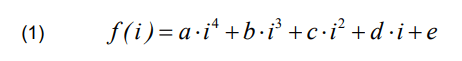
The basic values characterizing the annual variability of loads of both the electric power system and individual consumers are as follows: annual energy Ar, peak power Prs, average power Prśr, base load power Pro, annual peak power usage time Trs, average annual degree of load mrśr, degree of equalization of the base load lro, degree of basic load mro, peak equalization degree lrs, degree of uniformity of the monthly peaks σ’’r. These indicators are determined from the relation [2, 3, 8]:

where: Tr – average duration of the year (8760 h), Pmsi – peak power of the i-th month.
Table 1 presents the values of the designated coefficients for individual years being analyzed, while Figures 1 to 4 present selected charts thereof.
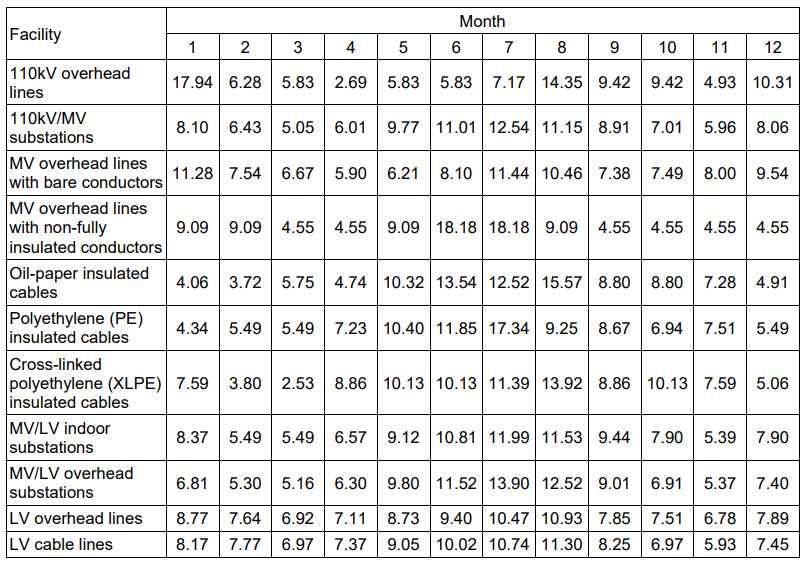
The annual load variation can also be presented in the form of monthly energy consumption. Figure 5 shows annual load schedules of the electric power system. Energy consumption continued to increase until 2018. However, after 2018, energy consumption decreased.
When analyzing the chart in Figure 5. it can be concluded that the electrical load is closely related to the season of the year. The load in winter is higher than in summer. In 2020, electricity consumption in December (the winter month with the highest energy consumption) was 15% higher than the electricity consumption in August (the summer month with the highest energy consumption). However, these differences have been decreasing significantly in recent years. In the first year of observation, the difference between the load during summer and winter was greater (22% of the difference) than after fifteen years, i.e. the last year of observation (15% of the difference). The differences in the load of the electric power grid are mainly due to the need to use lighting during the winter months. The fact that the number of electrical equipment we use has increased significantly over the last fifteen years may, however, have an impact on the equalization of loads. Today, almost every household is equipped with electrical appliances and gadgets that are used equally throughout the year. In addition, due to the occurrence of very high temperatures during summer, in recent years more and more private individuals and companies have decided to equip their houses and premises with air conditioners. Due to the increasing gasification of the country and access to modern and efficient boilers, fewer and fewer households use electricity for heating purposes in winter. Thermal renovations of buildings that reduce the demand for heat, including that generated by electricity, are also becoming more and more common. An important aspect is also the widespread replacement of energy-intensive light sources (such as incandescent lamps, sodium or mercury lamps) by energy-efficient light sources (such as LED or compact fluorescent lamps). This reduces power consumption, especially in autumn and winter.
Table 2 and figure 6 show an increase in household equipment with some electrical appliances. Today almost every consumer owns a mobile phone and a washing machine. There has also been a significant increase in the number of households equipped with dishwashers (from a few percent in 2006 to almost 40 percent in 2018) microwave ovens and computers (from around 40 percent at the beginning of the observation period to over 60 percent in the last year of observation). The chart in Figure 7 also shows the growing consumerism of our society which is increasing the energy consumption of households. Undoubtedly automation has also entered our homes and increasingly technologically advanced equipment is helping us to fulfill our daily chores. At present there are no statistics concerning the equipment of the inhabitants with commonly used gadgets and equipment such as game consoles, tablets, smart watches, music players, electric toothbrushes, slicers, multifunctional food processors, electric induction hobs, air purifiers etc. which also contribute to the increase of energy consumption by the municipal customers.
Table 1. Parameters and indicators characterizing the annual load variability [own study]
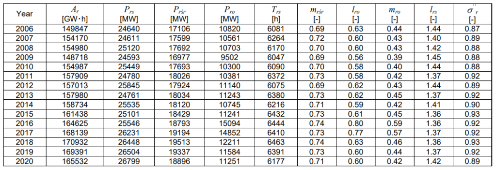
Table 2. Equipment of household population with certain durable goods [13]
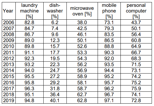
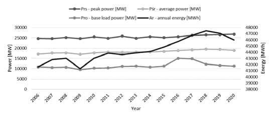
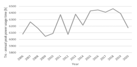


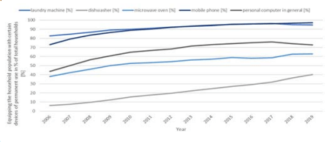
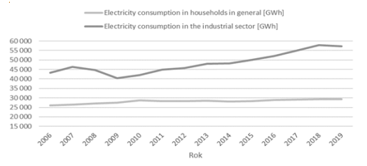
Table 3. Econometric models of the value of the base load degree [own study]

Econometric modeling of the value of the base load degree mro
Basic load degree mro determines the ratio of base load to peak load in a given calendar year thus characterizing the uniformity of loads.
An attempt was made to create an econometric model of the basic load degree mro which was determined on the basis of statistical data from Statistics Poland, the Energy Market Agency and PSE S.A. covering the years 2003-2017 [1, 13, 15].
Several hundred explanatory variables were selected. During the evaluation procedure. some of them were rejected and the variables that remained were related to household equipment. These are the ones that are most strongly correlated with the examined indicators (explanatory variables).
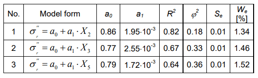
On the basis of extensive statistical surveys making a detailed analysis of the quantities affecting the value of the basic load degree mro. the following were adopted as explanatory variables for the model: X1 – equipment of households with washing machines [%], X2 – equipment of households with dishwashers [%], X3 – equipment of households with microwave ovens [%], X4 – equipment of households with mobile phones [%], X5 –equipment of households with personal computers [%].
The statistical procedure for selecting explanatory variables was then carried out. Quasi constant variables that do not contribute relevant information to the potential model were eliminated. The correlation coefficients of the explained variable mro with potential explanatory variables were calculated. Then from the set of potential explanatory variables, the variables that were poorly correlated with the response variable were eliminated. The variable that was most strongly correlated with the response variable was selected from among the remaining variables. The next step was to calculate the matrix of correlation coefficients between potential explanatory variables. The variables that were too strongly correlated with the previously selected explanatory variable, i.e. those that duplicated the information provided by it, were eliminated. The last stage of modeling consisted in the estimation of parameters of linear models using the least squares method. All the models developed were verified by determining the coefficient of determination R2 , the coefficient of convergence φ2 , the coefficient of random variability We and the standard estimation error Se.
Table 3 presents the comparison of the developed econometric models and their fitting measures.
Forecasting the value of the base load degree mro
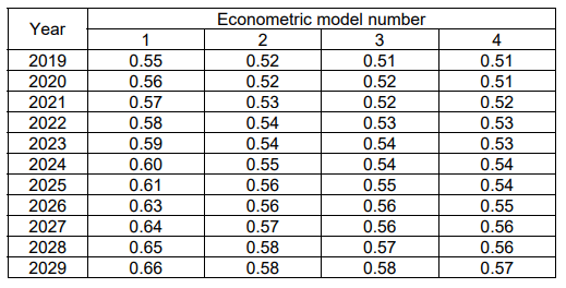
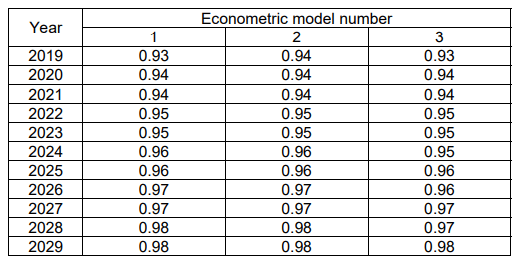
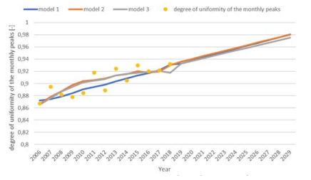
On the basis of the developed econometric models, a medium-term forecast of indicator mro for the years 2019- 2029 was made. Table 4 and Figure 8 present the forecast values. The forecasts were made on the assumption that the trend of all explanatory variables remains unchanged.
Table 4. Forecast values of the base load degree mro in 2019-2029 on the basis of developed econometric models [own study]

Econometric modeling of the value of the degree of uniformity of monthly peaks σ’’r
An attempt was also made to create an econometric model of the degree of uniformity of monthly peaks σ’’r which was determined on the basis of statistical data of Polish Power Grids Company covering the years 2006-2018 [8].
On the basis of extensive statistical surveys, making a detailed analysis of the quantities affecting the value of the degree of uniformity of monthly peaks σ’’r, the following were adopted as explanatory variables for the model: X1 – equipment of households with washing machines [%], X2 – equipment of households with dishwashers [%], X3 – equipment of households with microwave ovens [%], X4 – equipment of households with mobile phones [%], X5 – equipment of households with personal computers [%]. Table 5 presents the comparison of the developed econometric models and their fitting measures.
Table 5. Econometric models of the value of the degree of uniformity of monthly peaks
Forecasting the value of the degree of uniformity of monthly peaks σ’’r,
On the basis of the developed econometric models. a medium-term forecast of indicator σ’’r, for the years 2019- 2029 was made. Table 6 and Figure 9 present the forecast the trend of all explanatory variables remains unchanged.
Table 6. Forecast values of the degree of uniformity of monthly peaks σ’’r, in the years 2019-2029 calculated on the basis of developed econometric models [own study]
Conclusions
The conducted research concerns the annual variability of loads in the power system. On its basis, the following conclusions can be drawn.
1. In winter months the load is much higher than in summer months. However, the difference has been decreasing steadily in recent years. In the first years of observations, the ratio of the minimum load (occurring in summer) to the peak load (occurring in winter) was in the range of 0.39 – 0.44, in order to reach a value of even 0.59 in recent years.
2. The general load trend of the power system remains unchanged, i. e. the load in winter is higher than in summer. However, the parameters determining the value and dynamics of these changes are currently completely different than they were for example 10 – 15 years ago. As the analyzes carried out show, there is a trend of load balancing in the power system load. The ratio of base load power to peak load power increases slowly but steadily. This trend was very well illustrated by the realized econometric models.
3. Based on the theory of econometrics, the authors developed four models of the base load degree mro. These models allow an indicator to be determined on the basis of knowledge of publicly available statistical data. The first stage of the research was to select variables that could potentially affect the value of the indicator mro. Ultimately, the models are based on four statistical variables, namely: X2 – equipment of households with dishwashers [%], X3 – equipment of households with microwave ovens [%], X4 – equipment of households with mobile phones [%], X5 – equipment of households with personal computers [%].
4. The econometric models obtained are characterized by high reliability, as evidenced by high values of the coefficient of determination and low values of the standard estimation error. This means that the actual values of the base load degree mro differ from the theoretical values determined from the models by very small values, while the variability of the adopted explanatory variables largely explains the variability of the indicator mro.
5. On the basis of the developed models, a medium-term forecast of the value of the base load degree mro for the years 2019-2029 was made. The forecast values obtained for all the developed models, which are based on different statistical data, are similar.
6. On the basis of the forecasts made, it was noted that the indicator mro will grow over time. This indicates that the value of the base load power Pro will strive for the peak power value Pro. This will result in an increasing equalization of annual loads.
7. Based on the theory of econometrics, the authors also developed three models of the degree of uniformity of monthly peaks σ’’r. These models allow the indicator to be determined on the basis of knowledge of publicly available statistical data. The first stage of the research was to select variables that could potentially affect the value of the indicator σ’’r. Ultimately, the models are based on three statistical variables, namely: X2 – equipment of households with dishwashers [%], X3 – equipment of households with microwave ovens [%], X5 – equipment of households with personal computers [%].
8. The econometric models obtained are characterized by high reliability, as evidenced by high values of the coefficient of determination and low values of the standard estimation error. This means that the actual values of the degree of uniformity of monthly peaks σ’’r differ from the theoretical values determined from the models by very small values, while the variability of the adopted explanatory variables largely explains the variability of the indicator σ’’r.
9. On the basis of the forecasts made, it was noted that the indicator σ’’r will grow over time, striving asymptotically to the value of 1. This proves the equalization of monthly load peaks.
10. The analyses carried out show that increasing the equipment of households with a variety of everyday electrical appliances not only increases electricity consumption, but also balances the load of the power system.
11. The analysis showed that over the years, the difference in electricity consumption by season is decreasing. In the previous years. electricity consumption was much lower in summer than in autumn and winter months. At present, summer and winter loads are equalizing. This may be due to, among other things. common access to many electrical appliances and gadgets used on a daily basis and climate changes manifesting themselves in hot summers (the number of properties equipped with air conditioners is increasing). At the same time. due to the diversity of energy sources, the high summer load is easily covered by solar farms, for example, which produce the most energy during summer due to the highest solar irradiation. It should be stressed that there are many small and unstable energy sources (e. g. photovoltaic or wind farms) create real problems when balancing power in the power system.
12. High values of the correlation coefficient indicate that there is a significant dependence of the base load degree mro and the degree of uniformity of monthly peaks σ’’r on the level of equipment of households with electrical appliances. This confirms the thesis put forward in the introduction.
REFERENCES
[1] Agencja Rynku Energii, Statystyka Elektroenergetyki Polskiej, Warszawa (2003-2018)
[2] Chojnacki A. Ł. Analiza dobowej. tygodniowej i rocznej zmienności obciążeń elektroenergetycznych w sieciach miejskich oraz wiejskich. Przegląd Elektrotechniczny, Nr 6/2009, s. 56-61
[3] Chojnacki A. Ł., Kaźmierczyk A. Analiza dobowej i tygodniowej zmienności obciążeń mocą czynną i bierną elektroenergetycznych sieci dystrybucyjnych SN, miejskich oraz terenowych. Energetyka, Problemy Energetyki i Gospodarki Paliwowo-Energetycznej Nr 1/2011, s. 29-37
[4] Collins S. Deane P. Gallachóir B. Pfenninger S. Staffell I. Impacts of Inter-annual Wind and Solar Variations on the European Power System. Joule Volume 2. Issue 10, 17 October 2018, Pages 2076-2090
[5] Dobrzańska I., Dąsal K., Łyp J., Popławski T., Sowiński J., Prognozowanie w elektroenergetyce. Zagadnienie wybrane. Wydawnictwo Politechniki Częstochowskiej. Częstochowa 2002
[6] Góra S., Kopecki K., Marecki J., Pochyluk R. Zbiór zadań z gospodarki elektroenergetycznej. PWN. Warszawa 1976
[7] Majchrzak H. Problems related to balancing peak power on the example of the Polish National Power System. Archives of Electrical Engineering. Vol. 66(1), pp. 207-221 (2017)
[8] Matla R. Gospodarka elektroenergetyczna, Wydawnictwo Politechniki Warszawskiej, Warszawa (1977)
[9] Olauson J. Nasir Ayob M. Bergkvist M. Carpman N. Castellucci V. Goude A. Lingfors D. Waters R. Widén J. Net load variability in Nordic countries with a highly or fully renewable power system. Nature Energy vol. 1. Article number: 16175 (2016)
[10] Popławski T. (red), Dąsal K., Łyp J., Sowiński J. Wybrane zagadnienia prognozowania długoterminowego w systemach elektroenergetycznych. Wydawnictwo PCz. Częstochowa 2011
[11] Praca zbiorowa. Analiza I prognoza obciążeń elektroenergetycznyc. WNT. Warszawa 1971
[12] Sroka K. Złotecka D. The risk of large blackout failures in power systems, Archives of Electrical Engineering. Vol. 68(2). pp.411–426 (2019)
[13] Statistics Poland, Local Data Bank, https://bdl.stat.gov.pl/BDL/start accessed via the Internet on 14.10.2019
[14] Stępień J. C. Laboratorium gospodarski elektroenergetycznej, Wydawnictwo Politechniki Świętokrzyskiej, Kielce (1997)
[15] http://www.pse.pl – accessed on 21.11.2019
[16] http://www.weatheronline.pl – accessed on 28.11.2019
[17] Zidan A. El-Saadany E. F. Distribution system reconfiguration for energy loss reduction considering the variability of load and local renewable generation, Energy Vol. 59. 15 September 2013. Pages 698-707
Autorzy: mgr inż. Kornelia Banasik E-mail: k.banasik@tu.kielce.pl; dr hab. inż. Andrzej Ł. Chojnacki, prof. PŚk, E-mail: a.chojnacki@tu.kielce.pl, dr inż. Agata Każmierczyk E-mail: a.kazmierczyk@tu.kielce.pl, Politechnika Świętokrzyska, Katedra Energetyki, Energoelektroniki i Maszyn Elektrycznych, al. Tysiąclecia Państwa Polskiego 7, 25-314 Kielce
Source & Publisher Item Identifier: PRZEGLĄD ELEKTROTECHNICZNY, ISSN 0033-2097, R. 99 NR 1/2023. doi:10.15199/48.2023.01.12