Published by Mr. Thomas Ottosson, Managing Director, Unipower AB, Sweden. Email: thomas.ottosson@unipower.se . Website: unipower.se


Source URL: https://pqsynergy.com/assets/files/Power-QualityMeasurementsfromtheSpainPortugalBlackout.pdf
Published by Mr. Thomas Ottosson, Managing Director, Unipower AB, Sweden. Email: thomas.ottosson@unipower.se . Website: unipower.se
Source URL: https://pqsynergy.com/assets/files/Power-QualityMeasurementsfromtheSpainPortugalBlackout.pdf
Published by Mr. Jonny Carlsson, Research Manager, Unipower AB, Sweden. Email: jonny.carlsson@unipower.se . Website: unipower.se


Source URL: https://pqsynergy.com/assets/files/UNIPOWER-IEC61000-4-30Ed.4InprogressstateFDISMemberofWG9.pdf
Published by 1. Marwan R. Abed, 2. Oday A. Ahmed, 3. Ghassan A. Bilal, University of Technology Iraq, Baghdad, ORCID: 1. 0000-0002-1257-2810; 2. 0000-0001-7214-3412; 3. 0000-0002-5090-103X
Abstract. When implementing a DC distribution network, it is much easier to integrate distributed energy sources than it is with an ac grid. Furthermore, the efficiency and reliability of DC distribution networks outperform those of AC systems. The protection of the DC distribution networks, particularly the interruption and isolation of short-circuit fault currents, is still a major problem. Traditional mechanical and hybrid circuitbreakers for DC fault protection have the disadvantage of being sluggish to operate, necessitating the use of high-power equipment. The Solid-State Circuit Breaker is the best choice for quick fault interruption. Since they employ thyristors, Impedance-Source Circuit Breakers are among those that provide automated fault detection and clearing. In this work, a new DC circuit breaker based Δ-impedance source configuration is proposed for medium and low voltage DC distribution networks to provide the bidirectional operation which has also become the general requirement for the modern power system. The proposed topology uses three-coupled windings with one capacitor and four SCR thyristors to facilitate the bidirectional operation. MATLAB/Simulink environment is used to analyze and evaluate the performance of the proposed DC circuit breaker to protect the 240V DC microgrid configuration with different fault conditions and locations. The results obtained prove that the proposed DC circuit breaker has a good performance in protecting the DC distribution networks.
Streszczenie. Wdrażając sieć dystrybucyjną prądu stałego, znacznie łatwiej jest zintegrować rozproszone źródła energii niż z siecią prądu przemiennego. Ponadto wydajność i niezawodność sieci dystrybucyjnych prądu stałego przewyższa sieci prądu przemiennego. Ochrona sieci dystrybucyjnych prądu stałego, w szczególności przerywanie i izolowanie prądów zwarciowych, nadal stanowi poważny problem. Tradycyjne mechaniczne i hybrydowe wyłączniki automatyczne do ochrony przed zwarciami prądu stałego mają tę wadę, że działają wolno, co wymaga użycia sprzętu o dużej mocy. Wyłącznik półprzewodnikowy to najlepszy wybór do szybkiego przerywania zwarć. Ponieważ wykorzystują tyrystory, wyłączniki źródła impedancji należą do tych, które zapewniają automatyczne wykrywanie i usuwanie usterek. W tej pracy zaproponowano nową konfigurację źródła Δ-impedancji opartą na wyłączniku prądu stałego dla sieci dystrybucyjnych prądu stałego średniego i niskiego napięcia, aby zapewnić dwukierunkową pracę, która stała się również ogólnym wymogiem dla nowoczesnego systemu elektroenergetycznego. Proponowana topologia wykorzystuje trzy sprzężone uzwojenia z jednym kondensatorem i czterema tyrystorami SCR, aby ułatwić pracę dwukierunkową. Środowisko MATLAB/Simulink jest wykorzystywane do analizy i oceny wydajności proponowanego wyłącznika prądu stałego w celu ochrony konfiguracji mikrosieci 240 V DC z różnymi warunkami i lokalizacjami uszkodzeń. Uzyskane wyniki dowodzą, że proponowany wyłącznik prądu stałego ma dobrą skuteczność w zabezpieczaniu sieci dystrybucyjnych prądu stałego. (Zabezpieczenie mikrosieci DC za pomocą ΔCB)
Keywords: DC microgrid protection; Coupled inductor; DC circuit breaker; Bidirectional operation; Impedance source circuit breaker
Słowa kluczowe: ochrona mikrosieci prądu stałego; cewka sprzężona; wyłącznik prądu stałego; Działanie dwukierunkowe
The twentieth century began with a critical discussion over the form of energy supply and its essential elements. When Nikola Tesla with George Westinghouse argued for Alternating Current (AC) while Thomas Edison argued for Direct Current (DC). It was evident that the generation of DC power was restricted to a low voltage, and the voltage drop was a key concern. As a result, Edison’s power plants had to be used locally, which meant that loads had to be near the generating stations. The success of this fundamental milestone in the history of electricity notably ushered in the era of central power generation (power plants) and the global spread of AC transmission and distribution systems. In addition, power plants fuelled by fossil fuels (gas and coal) have risen to prominence as a source of electricity. To this time, AC power systems have lasted for even more than a century, and AC loads have ruled the market. However, high energy prices, as well as a lack of funds to build new big power stations with long-distance transmission networks, are some of the limitations to meet rising energy demand. Furthermore, ageing power system infrastructures, global warming, increased awareness of restricted power generation resources, higher power consumption requirements, and growth in the use of DC loads due to improvements in power electronics all indicate that transformation of the existing energy system is unavoidable [1, 2].
DC sources have been subjected to many developments causing an increment in the efficiency and live time of these sources, also the use of various DC loads, and the use of energy storage devices have led the way to use the of DC microgrids (DC MG). Harmonic, Ferranti, and skin effects are essentially non-existent in the DC-MG. As a consequence, DC MG will be better suited for new power systems than AC MG. The DC-MG idea may be viewed as a master foundation for using Smart Grid (SG) technologies [3]. The main problem in these DC MG is that the zerocrossing point is not present, so modern protection devices are needed to limit and interrupt the high fault current rapidly without producing sparks [4, 5].
The traditional mechanical DCCBs have many disadvantages such as Low current interruption abilities, slow response time, and low durability [5, 6], so a faster solid-state DCCBs have been suggested, these breakers provide a higher reliability and longer lifetime. The main disadvantage of such types of DCCBs are the demand for an additional forced commutation and sensing elements, which cause an increase in the circuit complexity and cost and also the high on-resistance (Ro) of the semiconductor switches [4-9].
The Impedance source DCCB is suggested as a faster response that isolates faults in microseconds and has an automatic turn-off because of its natural commutation principle [5, 10, 11].
In [11] produced the first unidirectional impedance source DCCB, consisting of one thyristor (SCR) and two capacitors and inductors which had been arranged as a cross shape. The absence of a common ground in the cross DCCB is solved by introducing the series ZCB in [10, 12]. Other research is done to reduce the reflecting current to zero and reduce the size and response time using coupled inductors in DCCBs as in [13]. In [14, 15] producing a symmetrical bidirectional ZCB with coupled-inductors. In [16, 17], a unidirectional Gamma DCCB (ГCB) was present. Also, in [18-22] presented the T-shape DCCBs (TCB). In [23-25] introduced a Y-shape DCCB (YCB), which consisted of a single capacitor and three coupled-inductors. The most important advantage of this configuration is the higher reflected current gain which produced by the secondary windings, as well as the three inductors’ turn ratios.
In this paper, a new symmetrical bi-directional with delta-shape coupled-inductors (ΔCB) is used in the protection of a DC MG, the following sections will introduce the new circuit breaker and test the protection of a 240V DC MG.
A new circuit breaker with three coupled inductors configuration, in which the inductors are connected in a delta shape, is introduced as a new impedance source CB. It also consists of a single capacitor and four SCRs arranged in two back-to-back switch pairs, as shown in Fig.1. The direction of power flow in the ΔCB is selected by the two switches in the gate circuit S1 and S2 as shown in Table.1.
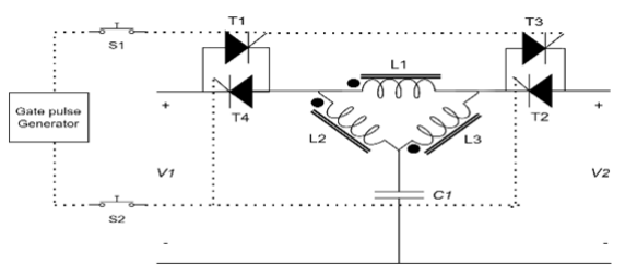
Table.1. Switches states of Gate circuit

Table.2. The values of the parameters of the proposed ΔCB

During steady state, the power flows from V1 to V2 through T1, L1, L2, L3, and T3, as shown in Fig.2. While the power flows from V2 to V1 through T4, L1, L2, L3, and T2 during opposite power flow direction, as illustrated in Fig.3. In the event of a transient situation, such as a short circuit fault or under sudden load change, the capacitor will act as the source that fed the transient current through the three delta-coupled inductors.


As shown in Fig.4, these inductors also act as a channel for the reflected current. If this reverse current is equal to a certain value of the forward current, it will force the thyristors to turn off immediately, causing an interruption to the source current.
By driving the current transfer relation of the ΔCB from the three loop equations, So the input-to-output current relation is shown in Eq.(1):
I1/I2=−𝑠(𝐿3−𝑀13+𝑀23)(𝐿3−𝑀31+𝑀32)+(𝐿1+𝐿2+𝐿3−𝑀12−𝑀13−𝑀21+𝑀23−𝑀31+𝑀32)(𝑠𝐿3+𝑅𝐿+𝑍𝑐)𝑠(𝐿2−𝑀12+𝑀32)(𝐿3−𝑀31+𝑀32)−(𝐿1+𝐿2+𝐿3−𝑀12−𝑀13−𝑀21+𝑀23−𝑀31+𝑀32)(𝑠𝑀32−𝑍𝑐)………Eq.(1)
Where: Zc: The total impedance of the capacitor By using the parameters in Table.2 to plot the bode plot of this relation, as shown in Fig.5:
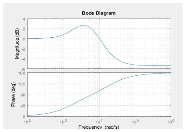
The figure shows a negative amplitude and higher value than the amplitude in low frequencies (steady state) with 180⁰ in phase. This reverse current will cause in a decrement in the first thyristor current making it lower than latching current, so the thyristor will turn-off causing in an interruption in the circuit breaker.
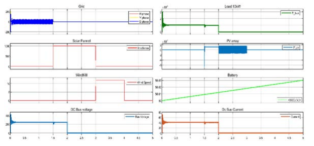
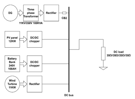
The ΔCB should be used to protect a DC microgrid (DCMG) from a short circuit fault. A MATLAB tool is used in this test. The simulation type is discrete of 5µs sampling time. A hybrid power supply system is constructed from three power sources: a connected AC grid, wind energy, and solar panels. The battery bank is 24v and used for transient cases during the changing from source to source and in an emergency. Every single source of the three power sources is regulated by a controller in order to provide a continuous supply to the load [26]. The sequence of the power source work in this simulation:
1. AC grid: From 0s to 1.5s.
2. Solar panel: From 1.5s to 3s.
3. Wind turbine: From 3s to 4s.
The schematic diagram of the used DCMG is shown in Fig.6. The bus voltage of the DCMG is 250V and the load consists of four parallel loads 30Ω, 20Ω, 20Ω, and 30Ω (the total load is equal to 6Ω), the load is connected to the DC bus.

a) The CB is in series with the load
The system is tested under normal operation and records the voltage and current of each power source, bus voltage, and load current (Ibus=ILoad). The simulation time is 5s. The steady-state results are obtained Fig.7.

Three different fault cases will be tested, as follows:
The first fault case: By inserting the fault after one second from a run during the period of the AC grid supply source, The AC is converted to DC through the rectifier and the inductive filter, and the load current shows the isolation of the breaker in about 10µs as shown in Fig.8 (Ibus=ILoad), and the other results are obtained as shown in Fig.9.
The second case: By inserting the fault after two seconds from the simulation run during the PV panel (solar panel) supply source period, Also, the load current shows the isolation of the breaker in about 10µs as shown in Fig.10, and the results are obtained as shown in Fig.11.


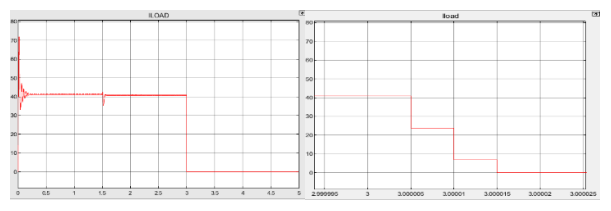

The third case: By inserting the fault after three seconds from a run during the period of the wind turbine and its rectifier as a supply source, the load current shows the isolation of the breaker in about 10µs as shown in Fig.12, and the results are obtained as shown in Fig.13.
b) The CB is in series with the rectifier of the AC Grid
The ΔCB is connected in series with the filter of the AC grid, as shown in Fig.14. The fault occurs after 0.5 seconds, and the source current of the ΔCB interrupted after 4.1ms with an overshoot during transient, as shown in Fig.15. The delay in isolation time and the increment in the current overshoot are because of the ripple in the rectified power and the effect of the inductor used as a filter.

Adding a capacitor in parallel with the input of this ΔCB of 220µF will illuminate the overshoot problem, and the isolation time will be reduced to 35µs, as shown in Fig.16.


MATLAB/Simulink environment is used to analyze and evaluate the performance of the proposed DC circuit breaker to protect the 240V DC microgrid configuration with different fault conditions and locations. The results prove that the proposed DC circuit breaker is well at protecting the DC distribution networks. It shows a faster isolation time of 10µs and no negative part in the source current. That makes it the better choice for protecting DC microgrids. Finally, the result shows that ΔCB could distinguish between fault and step load change.
REFERENCES
[1] D. Kumar, F. Zare, and A. Ghosh, “DC microgrid technology: system architectures, AC grid interfaces, grounding schemes, power quality, communication networks, applications, and standardizations aspects,” Ieee Access, vol. 5, pp. 12230-12256, 2017.
[2] J. J. Justo, F. Mwasilu, J. Lee, and J.-W. Jung, “AC-microgrids versus DC-microgrids with distributed energy resources: A review,” Renewable and sustainable energy reviews, vol. 24, pp. 387-405, 2013.
[3] K. Nandini, N. Jayalakshmi, and V. K. Jadoun, “An overview of DC Microgrid with DC distribution system for DC loads,” Materials Today: Proceedings, 2021.
[4] W. Li, Y. Wang, X. Wu, and X. Zhang, “A novel solid-state circuit breaker for on-board DC microgrid system,” IEEE Transactions on Industrial Electronics, vol. 66, no. 7, pp. 5715-5723, 2018.
[5] S. S. Lumen, R. Kannan, and N. Z. Yahaya, “DC Circuit Breaker: A Comprehensive Review of Solid State Topologies,” in 2020 IEEE International Conference on Power and Energy (PECon), 2020: IEEE, pp. 1-6.
[6] S. Bhatta, R. Fu, and Y. Zhang, “A New Design of Z-Source Capacitors to Ensure SCR’s Turn-Off for the Practical Applications of ZCBs in Realistic DC Network Protection,” IEEE Transactions on Power Electronics, vol. 36, no. 9, pp. 10089-10096, 2021.
[7] S. Bhatta, “Specification, Control, and Applications of Z-Source Circuit Breakers for the Protection of DC Power Networks,” 2021.
[8] V. Raghavendra, S. N. Banavath, and S. Thamballa, “Modified z-source dc circuit breaker with enhanced performance during commissioning and reclosing,” IEEE Transactions on Power Electronics, vol. 37, no. 1, pp. 910-919, 2021.
[9] L. L. Qi, A. Antoniazzi, L. Raciti, and D. Leoni, “Design of solidstate circuit breaker-based protection for DC shipboard power systems,” IEEE Journal of Emerging and Selected Topics in Power Electronics, vol. 5, no. 1, pp. 260-268, 2016.
[10] A. H. Chang, B. R. Sennett, A.-T. Avestruz, S. B. Leeb, and J. L. Kirtley, “Analysis and design of DC system protection using Z-source circuit breaker,” IEEE Transactions on Power Electronics, vol. 31, no. 2, pp. 1036-1049, 2015.
[11] K. A. Corzine and R. W. Ashton, “A new Z-source DC circuit breaker,” IEEE Transactions on Power Electronics, vol. 27, no.6, pp. 2796-2804, 2011.
[12] A. H. Chang, A.-T. Avestruz, S. B. Leeb, and J. L. Kirtley, “Design of dc system protection,” in 2013 IEEE Electric Ship Technologies Symposium (ESTS), 2013: IEEE, pp. 500-508.
[13] A. Maqsood and K. Corzine, “Z-source Dc circuit breakers with coupled inductors,” in 2015 IEEE Energy Conversion Congress and Exposition (ECCE), 2015: IEEE, pp. 1905-1909.
[14] S. G. Savaliya and B. G. Fernandes, “Modified bi-directional Zsource breaker with reclosing and rebreaking capabilities,” in 2018 IEEE Applied Power Electronics Conference and Exposition (APEC), 2018: IEEE, pp. 3497-3504.
[15] S. G. Savaliya and B. G. Fernandes, “Performance Evaluation of a Modified Bidirectional Z-Source Breaker,” IEEE Transactions on Industrial Electronics, vol. 68, no. 8, pp. 7137-7145, 2020.
[16] H. Al-khafaf and J. Asumadu, “Γ-Z-source DC circuit breaker operation with variable coupling coefficient k,” in 2017 IEEE International Conference on Electro Information Technology (EIT), 2017: IEEE, pp. 492-496.
[17] X. Diao, F. Liu, Y. Song, M. X. Y. Zhuang, and X. Zha, “Topology Simplification and Parameter Design of Z/T/CSource Circuit Breakers,” IEEE Journal of Emerging and Selected Topics in Power Electronics, 2021.
[18] C. Li, Z. Nie, H. Li, and Y. Zhang, “A novel solid-state protection scheme for DC system,” in 2016 IEEE 8th International Power Electronics and Motion Control Conference (IPEMC-ECCE Asia), 2016: IEEE, pp. 2039-2042.
[19] Y. Song, Y. Yu, S. Wang, Q. Liu, and X. Li, “A Novel Efficient Bidirectional T-source Circuit Breaker for Low Voltage DC Distribution Network,” in 2021 IEEE 12th International Symposium on Power Electronics for Distributed Generation Systems (PEDG), 2021: IEEE, pp. 1-5.
[20] X. Diao, F. Liu, Y. Song, M. Xu, Y. Zhuang, and X. Zha, “An Integral Fault Location Algorithm Based on a Modified T-source Circuit Breaker for Flexible DC Distribution Networks,” IEEE Transactions on Power Delivery, 2020.
[21] S. Sapkota, K. Pokharel, Y. Wang, W. Li, and H. Wang, “Modified T-Source Circuit Breaker for Bidirectional Operation in MVDC,” in 2020 IEEE Sustainable Power and Energy Conference (iSPEC), 2020: IEEE, pp. 813-818.
[22] X. Diao, F. Liu, Y. Song, M. X. Y. Zhuang, W. Zhu, and X. Zha, “A New Efficient Bidirectional T-source Circuit Breaker for Flexible DC Distribution Networks,” IEEE Journal of Emerging and Selected Topics in Power Electronics, 2020.
[23] H. Al-Khafaf and J. Asumadu, “Bi-directional Y-Source DC Circuit Breaker Design and Analysis Under Different Conditions of Coupling,” in 2018 9th IEEE International Symposium on Power Electronics for Distributed Generation Systems (PEDG), 2018: IEEE, pp. 1-6.
[24] H. Al-khafaf and J. Asumadu, “Efficient Protection Scheme Based on Y-Source Circuit Breaker in Bi-Directional Zones for MVDC Micro-Grids,” Inventions, vol. 6, no. 1, p. 18, 2021.
[25] H. Al-khafaf and J. Asumadu, “Y-source bi-directional dc circuit breaker,” in 2018 International Power Electronics Conference (IPEC-Niigata 2018-ECCE Asia), 2018: IEEE, pp. i-v.
[26] D. SHAH. “DESIGN OF DC MICROGRID.” MathWorks. https://www.mathworks.com/matlabcentral/fileexchange/104120-design-of-dc-microgrid (accessed March 4, 2023).
Source & Publisher Item Identifier: PRZEGLĄD ELEKTROTECHNICZNY, ISSN 0033-2097, R. 99 NR 11/2023. doi:10.15199/48.2023.11.25
Published by Dranetz Technologies, Inc., Case Study
Utility energy and demand costs have a direct impact on a company’s bottom line. In fact, a typical commercial or industrial facility can save from 10% to as much as 35% annually on energy costs by implementing a comprehensive energy management plan. And while each facility will require an organized approach to recognize those savings, facilities first need to understand their power consumption, location of major loads, electric demand usage patterns, and associated costs.

The cost of energy is one of the most commonly mismanaged expenses, regardless of a company’s size or the industry represented. Often, energy is purchased in one department, consumed in another, with energy management systems operated and maintained by still another. Since each facility’s energy situation is dynamic and interdependent, it requires continuous monitoring and management action to avoid escalating costs. The web-based Signature System™ enables users to continuously monitor and store power consumption and quality information in real time-to capture those savings and improve profitability. Customers use the System for:
Power cost management: By looking at time of day, peak load and aggregated energy usage, customers can reduce their costs by rescheduling loads, making sure unneeded equipment is shut off when not in use, or installing energy-efficient equipment. Historical load profile data can be used to develop price/risk curves for evaluating energy purchase agreements.
Power factor: Many customers pay a penalty to the utility for inefficient use of energy, or the ratio of power consumed to power delivered. Monitoring is a necessary tool for understanding the processes within a facility that impact power factor, to improve energy efficiency and reduce or eliminate any surcharges.
Curtailment Rate Structure: Many customers have agreed to reduce (curtail) load at the request of their utility supplier in exchange for lower energy rates. Plus, non-essential loads can be shed or distributed generation brought on line to reduce consumption and/or participate in utility-sponsored demand reduction programs. Monitoring can help determine which loads on which circuits can be curtailed, as well as to certify compliance with curtailment requests.
Allocate Costs and Perform Activity-based Costing: Track energy-related costs by department, tenant or process. Use the Signature System’s Energy Usage and Expense Reporting AnswerModule® to track, compare and document those costs against scheduled rates, and from one time period to another.
Load profiling: Adding or upgrading equipment, computers and processes will impact the power requirements of a facility. Monitoring the existing load on circuits lets you know the impact of those changes and how much new load can be added to an existing circuit or facility.
Lost power costs: Improper load balance grounding may not always be obvious. By monitoring, lost energy can be identified and minimized.
Source URL: https://www.dranetz.com/technical-support-request/case-studies/case-study-manage-energy-expenses/
Dranetz Products: Dranetz HDPQ® Plus & SP Family
Website: Dranetz.com , Call 1-800-372-6832 (US and Canada) or +1-732-287-3680 (International)
Published by Dranetz Technologies, Inc., Technical Documents
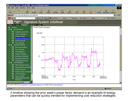
he HDPQ Family of products have a number of trigger mechanisms for capturing different types of power quality phenomena. Most users are familiar with settings for sags and swells, but those typical limits usually don’t capture the “blinky lights” problems. While the Pst (perceptibility short term) parameter will indicate whether the voltage supply is likely to produce light flicker when the Pst is close or above 1, it doesn’t help determine where it comes from or what the source is since it is a ten-minute journal value. The graph below illustrates such.

The voltage and current plots show that it is an increase in current over 100A that results in the voltage decreasing by 5-8V every 15 minutes. The rms variation limit for sags is set to 90% of the nominal 120V or 108V, so no sag was reported. In above example, the red dotted line is that sag limit. Yet the residents complained of “blinky lights” while the Pst does increase to 0.8 each time, not over 1.
The rms deviation transient trigger is one method to capture such as an event. However, there is a parameter that is included in the IEC and IEEE standards that was defined just for such disturbances. It is the RVC or Rapid Voltage Change. It looks for a sudden change in the voltage from one steady state value, waits for stability in any continued variations until stable at another steady state voltage value for 1 second or more. The delta change limit is typically set to 2-3%. Since the variation shown in the data above was 4-7%, this mechanism was ideal for capturing and reporting each time that it happened. An example at 22:189:54 is shown below. The rms deviations and wave shape triggers also captured the event, but they also triggered on other disturbances that weren’t part of the investigation, which produced extra data to sort through.
#39 10/03/2017 22:02:05.297 AV Misc at 0.8 Deg
#40 10/03/2017 22:02:05.297 BV Misc at -179.1 Deg
#41 10/03/2017 22:02:05.306 AVRmsDev Normal To High
#42 10/03/2017 22:02:05.306 BVRmsDev Normal To High
#44 10/03/2017 22:02:05.323 AVRmsDev High To Normal
#45 10/03/2017 22:02:05.323 BVRmsDev High To Normal
#48 10/03/2017 22:18:54.874 AV Misc at 0.7 Deg
#49 10/03/2017 22:18:54.874 BV Misc at -179.0 Deg
#50 10/03/2017 22:18:54.874 AVRmsDev Normal To High
#51 10/03/2017 22:18:54.874 BVRmsDev Normal To High
#52 10/03/2017 22:18:54.883 A Delta V RVC Rapid Voltage Change 0.175 Sec.
#53 10/03/2017 22:18:54.883 B Delta V RVC Rapid Voltage Change 0.259 Sec.
The right tool for the right job has always been a wise adage. Setting the right tool up with the right limits on the right parameters to help solve the customer’s problems is an extension of that idea that can help get the answer quickly and clearly. By the way, the answer here was a common answer for such problems. The HVAC unit was causing the blinky lights.
Source URL: https://www.dranetz.com/technical-support-request/technical-documents/investigating-blinky-lights/
Dranetz Products: Dranetz HDPQ® Plus & SP Family
Website: Dranetz.com , Call 1-800-372-6832 (US and Canada) or +1-732-287-3680 (International)
Publised by Oleh HOLOVKO1, Adam KONIECZKA2, Adam DĄBROWSKI3, Politechnika Poznańska, Wydział Automatyki, Robotyki i Elektrotechniki (1, 2, 3)
ORCID: 2. 0000-0002-0362-3006; 3. 0000-0002-9385-6080O
Abstract. This paper proposes a method for evaluating the efficiency of passive cooling systems of solar panels in a type of radiator using CFD simulations. The movement of air through the cooling system and the dependence of the thermal state of the radiator on its shape, wind speed, and ambient temperature were analyzed. A mathematical analysis was made that takes into account the average temperature drop of a solar panel connected to a ribbed heat sink. Experimental measurements of the temperature of the solar panel were performed.
Streszczenie. W artykule zaproponowano metodę oceny wydajności pasywnych układów chłodzenia paneli fotowoltaicznych bazujących na radiatorach z wykorzystaniem symulacji CFD. Przeanalizowano ruch powietrza w układzie chłodzącym oraz zależność temperatury radiatora od jego kształtu, prędkości wiatru i temperatury otoczenia. Przeprowadzono analizę matematyczną uwzględniającą spadek średniej temperatury panelu fotowoltaicznego połączonego z żebrowym radiatorem. Wykonano eksperymentalne pomiary temperatury panelu fotowoltaicznego. (Modelowanie systemów chłodzenia pasywnego paneli fotowoltaicznych).
Słowa kluczowe: panel solarny; wydajność paneli solarnych; radiator; symulacje CFD.
Keywords: solar panel; efficiency of solar panels; heat sink; CFD simulations.
According to [1], an increase in the installed capacity of photovoltaics in Poland amounted in 2021 to 3.7 GW. Data from the end of the first quarter of 2022 indicates the installed power of 9.4 GW. The global success of the solar industry is due to many factors but reduction of the cost of the generated electricity is crucial: according to [2] (Fig. 1), the cost of solar energy over the past 10 years has fallen 7.5 times.

The second reason is versatility: from small housing systems to large enterprises. In addition, unlike fossil-fuel electricity generation, solar energy causes no environment damage.
The main task with the use of solar radiation is to increase the efficiency of solar panels. The efficiency of commonly used photovoltaic panels is between 17 and 24% [3]. Most commonly used solar cells use wavelength range of 250 to 1100 nm to generate electricity. The remaining radiation is reflected or absorbed by the cells as heat. The temperature of the solar panel is influenced by external climatic variables such as wind speed, humidity, atmospheric temperature and concentrated dust [4]. The heat emission from the roof surface also plays an important role. The absorbed heat may raise the panel temperature even up to 70‒80°C. The result is a significant decrease in the output power.
The amount of energy loss of photovoltaic modules as a result of overheating shall be determined during the production tests. The thermal power loss in different models of silicon-crystalline batteries (according to the manufacturers’ catalog data) is on average within the limits of 0.45 to 0.50%/°C. Thin-film (amorphous) solar panels are more resistant to temperatures. Their thermal loss performance is about 0.2–0.3%/°C [5]. A way to improve the performance of solar panels is to keep their temperature within the optimum range. This method will not only increase electricity generation but also extend the life of the modules, which currently stands at 25 years.
There are many ways to cool solar panels:
1) Active cooling is carried out by forced air or liquid in both the area of the panel itself and the heat exchangers installed on the panels [6]. Problems with the use of active systems are mainly related to: additional equipment, which, as a rule, is not agreed upon with the manufacturer and additional costs of calculations, installation, maintenance. When using liquid-cooled systems, there is a problem of maintaining the installation in the winter to avoid damage.
2) Passive methods include panel cooling using phase conversion materials, heat pipes and radiators: conventional and micro-channel heat exchangers, nanofluids, spectral filters, and thermoelectric, evaporative and radiation cooling [6].
The method of natural cooling has great potential, does not require energy supply and is reliable and simple. In [7], based on the modeling results, the area of an additional surface needed to compensate for the heating of a solar panel was calculated. The size of the additional surface area should be 5‒5.5 times the size of the solar cell. However, the performed calculations do not take the shape of the cooling surface and the relative direction of the wind into account.
According to [8‒11], the use of a passive cooling system in the form of a radiator (aluminum or copper fins mounted on the back of the solar panel) allows the average temperature of the solar panel to be reduced by 2 to 7°C, thus raise its efficiency by 2‒4%.
In [12, 13] the efficiency of a radiator with perforated ribs was considered, and in [14‒17], a study of inclined and complex-shaped ribs was carried out. Depending on the geometry of the structure and wind speed, the temperature of the solar panel decreases by 4‒12 degrees. It should be noted that the measurements and calculations in the mentioned works were carried out for specific locations of solar panels and cannot be applied to other places and conditions.
The degree of the temperature drop depends on the characteristics and location of the panel, stochastic climatic conditions, the design used and the material of the cooling system. In order to estimate the magnitude of the temperature drop of a photovoltaic panel achieved with a heat sink, a full detailed analysis of the airflow shall be carried out, taking the effect of gravity into account, the design of the heat sink, the position and orientation of the panel and other objects near the panel.
CFD (Computational Fluid Dynamics) method can be used for modeling active and passive cooling systems. This method needs numerical analysis to analyze and solve fluid flow problems. In papers [18–21] thermal analysis of the heat sink in the conditions of air convection was considered. In [19] the CFD simulation results were compared with experimental results. Heat transfer tests were carried out for various shapes of radiators (solid pin fins, perforated pin fins, solid flat plate, and perforated flat plate). The achieved results show that the base temperature for experiment is typically 6.05% to 9.52% higher than the base temperature of the CFD simulation. Therefore, the use of CFD software for modeling parameters of heat transfer in passive cooling of solar panels in real conditions can be reasonable.
Section 2 presents the methodology for estimating and theoretical calculations of the temperature drop of a solar panel with a passive cooling system depending on the type of heat sink and external conditions (wind direction and speed). For this purpose the CFD modeling software Solidworks Flow Simulation was used. It allows for performing a simulation of fluid flow, advanced thermal analysis, and study of heat exchange between the designed components and the predefined medium.
Section 3 presents experimental verification of the temperature dependence of a photovoltaic panel without cooling and with a passive cooling system in the form of a rib radiator on external climatic conditions. A thermal imaging camera was used for experimental testing.
A brief summary and conclusions are provided in Section 4.
Table 1. Selected theoretical and statistical models to determine the temperature of a photovoltaic cell
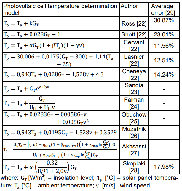
When calculating the temperature of the solar panel, the most influential factors are usually taken into account: the power of the solar radiation falling on the surface of the module, the ambient temperature and the wind speed. To determine the T୮ (temperature of the photovoltaic cell), various theoretical and statistical models have been proposed, determining the appearance, respectively [22‒28]. Table 1 shows commonly used T୮ calculation equations. However (according to [29]) depending on the chosen thermal model, the average error between the calculations and the measured value of the solar panel temperature can reach more than 30 percent.
The choice of a model and appropriate coefficients depends on the type of the panel and the conditions under which the panel is located. It can be determined from experimental data [30].
To analyze radiator performance, various ribbed radiators were modeled in Solidworks 3D CAD (2017), assuming that they are made of 5052-type aluminum alloy (thermal conductivity 140 W/mK (T=273K), density ‒ 2680 kg/m3 , specific heat ‒ 921 J/kg·K) [31].
During modeling, the following parameters were determined:
• P [W] ‒ total heat transfer capacity,
• Q [W/m2] ‒ the amount of heat distributed by the radiator surface unit,
• T [°C] ‒ initial temperature of the front surface of the heat sink,
• Tm [°C] ‒ average temperature of the heat sink,
• Tmin [°C] ‒ m
An example of the simulation obtained for a rib radiator is shown in Fig. 2.

Geometric dimensions of the heat sink affect the amount of dissipated heat. The purpose of the prepared tests is to perform a comparative analysis of heat exchange efficiency for the rib-type radiators with different rib heights ‒ L [mm].
Figure 3 summarizes the heat transfer efficiency of radiators of different shapes. The wind speed varied within 0‒ 20 m/s, the direction of air flow was perpendicular to the ribs at the rear, overheating of the front of the module in relation to the environment is 40°C.
Analysis of the dependence of the heat dissipation power on the surface of the radiator shows that under certain conditions the most efficient are radiators with a rib height of 20‒35 mm, providing a decrease in the module temperature on average from 5.74 to 11.8°C.
Compared to a flat plate of 5052-type aluminum alloy, the average heat dissipation power of the radiator increases 3.13 and 3.30 times, respectively. No further increase in the dimensions is recommended, since a significant part of the radiator does not participate in heat exchange with the environment.
Further tests shall aim to determine the optimum position of the radiator relative to the wind direction at different initial temperatures of the front panel.
Analysis of the heat dissipation efficiency of an unshielded radiator Q [W/m2] (Fig. 4) shows that the most efficient system is one in which the flows are directed perpendicular to the radiator from the ribs (100%) or along the ribs (99%). Changing the wind direction – from the front of the photo module (direction Z) or perpendicular to the ribs (direction X) – causes a decrease in efficiency by 55% and 40%, respectively.

The reason for such a decrease in the efficiency of the radiator as a cooling system is a significant decrease in wind speed in the area of the ribs. Figure 5 shows an example of the temperature distribution on the surface of the radiator and wind speed values in the radiator area.
In the next step, the dependences of the average temperature of the heat sink on the temperature difference between the heat sink and the surrounding air, wind speed and direction at the location of the panel were analyzed.
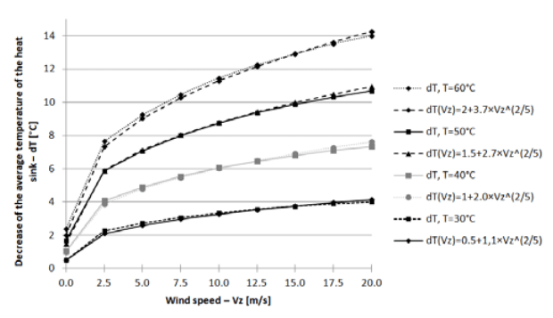
Figure 6 shows an illustrative calculation of the average heat sink temperature Tm[°C] for a radiator of dimensions 35×75×100 mm (s=0,063 m2) as a function of the initial temperature of the front surface T[°C] of the solar panel and wind speed. The influence of the thermal resistance between the solar panel and the radiator has not been taken into account.


The magnitude of the decrease in the average temperature of the radiator can be described using a mathematical function. Considering the above simulation, the decrease in the average temperature dTm[°C] at different temperatures T[°C] of the initial front surfaces can be described using the proposed mathematical expression

where σ, τ [°C ∙ s/m], λ[s/m] , m, n are determined using nonlinear regression of CFD simulation results.
For example, when using a radiator with the rib thickness of 1 mm, the rib height of 35 mm, the distance between the ribs of 7.5 mm and the wind direction perpendicular to the radiator from the side of the ribs, the coefficients have the following values:

Figure 7 for a radiator (35×75×100 mm s=0.063 m2) shows the simulation dependence and proposed mathematical expression of the decrease in the average temperature of the dT[°C] on the wind speed, the temperature T[°C] of the initial front surface.
The Sandia thermal model [23] was used to calculate the theoretical temperature, which corresponds to experimental data for a SYP-S05V5W solar panel used in research [31].

The corresponding coefficients for a panel with a polymer substrate are: ε = 1 [K∙m2/W], a = -3.56, b = -0.075 s/m [23].
For an unshielded photovoltaic panel installed at an angle of 45°, taking into account the average wind direction in the Wielkopolska ‒ region south-west (at an angle of 45° at the rear of the solar panel), the coefficients in equation (1) (according to the next Solidworks Flow Simulation) determining the temperature decrease have the following values:

The use of an additional cooling module reduces the average temperature of the entire system (panel and heatsink). In this work a proportional dependence of the change in the average temperature of the solar panel with the cooling system on the temperature of the illuminated side it is assumed. This change can be recorded with a thermal imaging camera.
An experimental verification of the temperature dependence of a photovoltaic panel without heat sink and with a passive cooling system on external climatic conditions was carried out on 17th January 2022 in a place with coordinates 52.4028 and 16.9537 [31].
A radiator with dimensions of (35×75×100 mm) was vertically placed on the right hand side of the solar panel type SYP-S05V5w, the angle of inclination of the panel was 40°, the wind speed during the day varied within the limits (6‒12 m/s). The temperature during the day varied between +2 and +11°C, with an average of +8°C. Information about the level of solar radiation, ambient temperature, and wind speed comes from the internet weather service [32] and additionally from the NASA MERRA-2 model [33].
A detailed temperature measurement of the panel and radiator was performed using the Seek Thermal ShotPRO thermal imaging device. Figures 8 and 9 show a photo of the solar panel taken with a thermal imaging camera.

The reduction of the mean temperature of the solar panel was calculated according to model (1) for the uncovered ribbed radiator (2).
Figure 10 shows theoretical calculations of the temperature of the panel without cooling and with a passive cooling system during the day and experimental measurements of the temperature of the solar panel using the above thermal imaging camera. Analysis of this chart shows a good match between the theoretical calculations and the experimental data.

The average temperature of the module during the day without a cooling system is 12.3°C, while with the cooling system the theoretical temperature is 11.0°C and the experimental temperature is 10.2°C.
The use of Solidworks Flow Simulation to CFD modeling of solar panels allows one to evaluate the thermal state of photovoltaic panels and the effectiveness of a passive cooling system of any material, size and shape.
The coefficients σ, τ,λ, m, n in expression (1) determining the temperature drop using a radiator are depending on its design, the angle of inclination of the solar panel, the direction of the wind at the location of the panel, the distance to the limiting planes (other panels) and can be determined on the basis of the performed simulation.
Application of the proposed method for estimation of the thermal state of solar panels with a passive cooling system enables estimation of the energy production of solar panels installed in any location at a defined time.
The research was financed by a research grant 0211/SBAD/0223.
REFERENCES
[1] Rynek Fotowoltaiki w Polsce 2022 (Photovoltaic market in Poland 2022), https://ieo.pl/pl/raport-pv 2022, access: 15.03.2022.
[2] SolarPower Europe, Global Market Outlook for Solar Power 2021‒2025, https://www.solarpowereurope.org/global-marketoutlook-2021-2025/, access: 20.7.2021.
[3] Photovoltaic Energy Factsheet, Center for Sustainable Systems, University of Michigan. 2022, Pub. No. CSS07-08.
[4] Siecker J., A review of solar photovoltaic systems cooling technologies, Renew. Sustain. Energy Rev. 79 (2017) 192-203.
[5] Sayigh A., Comprehensive Renewable Energy, Photovoltaic Solar Energy, Volume One, Elsevier Ltd, 2012, P.746.
[6] Sato D., Yamada N., Review of photovoltaic module cooling methods and performance evaluation of the radiative cooling method, Renew. Sustain. Energy Rev. 104 (January) (2019), 151-166.
[7] Асанов М.М., Бекиров Э.А., Воскресенская С.Н., Снижение влияния нагрева поверхности фотоэлемента на эффективность его работы (Reducing the effect of solar cell surface heating on its efficiency), Строительство итехногенная безопасность, No 51. (2014), pp. 92-96.
[8] Parkunam N., Pandiyan L., Navaneethakrishnan G., Arul S., Vijayan V., Experimental analysis on passive cooling of flat photovoltaic panel with heat sink and wick structure, Energy Sources, Part A Recovery, Util. Environ. Eff. (2019), https://doi.org/10.1080/15567036.2019.1588429.
[9] Firoozzadeh M., Shiravi A.H., Shafiee M., An experimental study on cooling the photovoltaic modules by fins to improve power generation: economic assessment, Iranian (iranica), Journal of Energy and Environment 10(2) (2019) 80-84, https://doi.org/10.5829/ijee.2019.10.02.02.
[10] El Mays A., et al., Improving photovoltaic panel using finned plate of aluminum, Energy Procedia, 119 (2017) 812-817.
[11] Chen H., Chen X., Li S., Ding H., Comparative study on the performance improvement of photovoltaic panel with passive cooling under natural ventilation, Int. J. Smart Grid Clean Energy, (2014), https://doi.org/10.12720/sgce.3.4.374-379.
[12] Arifin Z., Danardono Dwi Prija Tjahjana D., Hadi S., et. al., Numerical and experimental investigation of air cooling for photovoltaic panels using aluminum heat sinks, Int. J. Photoenergy (2020), 1574274, https://doi.org/10.1155/2020/1574274.
[13] Gotmare J.A., Borkar D.S., Hatwar P.R., Experimental investigation of PV panel with fin cooling under natural convection, Int. J. Adv. Technol. Eng. Sci., 03 (02) (2015) (February).
[14] Bayrak F., Oztop H.F., Selimefendigil F., Effects of different fin parameters on temperature and efficiency for cooling of photovoltaic panels under natural convection, Sol. Energy, 188 (2019) 484-494.
[15] Hernandez-Perez J.G., Carrillo J.G., et. al., Thermal performance of a discontinuous finned heatsink profile for PV passive cooling, Applied Thermal Engineering, 184 (2021) 116238, https://doi.org/10.1016/j.applthermaleng.2020.116238.
[16] Popovic C.G., Hudis teanu S.V., Mateescu T.D., Chereches N.- C., Efficiency Improvement of Photovoltaic Panels by Using Air Cooled Heat Sinks, Energy Procedia, 85 (2016) 425-432.
[17]Jobair H., Improving of photovoltaic cell performance by cooling using two different types of fins, International Journal of Computer Applications (0975–8887), Volume 157 – No 5, (2017) (January)
[18] Freegah B., Hussain A.A., Falih A.H., Towsyfyan H., CFD analysis of heat transfer enhancement in plate-fin heat sinks with fillet profile: Investigation of new designs, Therm. Sci. Eng.Prog., 17 (December) (2019), p. 2020, DOI: 10.1016/j.tsep.2019.100458.
[19] Tijani A.S., Jaffri N.B., Thermal analysis of perforated pin-fins heat sink under forced convection condition, Procedia Manuf., 24 (2018), pp. 290-298, DOI: 10.1016/j.promfg.2018.06.025.
[20] Pal V., Modeling and thermal analysis of heat sink with scales on fins cooled by natural convection, Int. J. of Research in Eng. and Technology, 03(06), 2014, pp. 359-362, DOI: 10.15623/ijret.2014.0306067.
[21] Parihar S., Randa R., Thermal Analysis of Heat Sink Using Solidworks, J. of Emerging Technologies and Innovative Research (JETIR), 8 (10), 2021, pp. 167-175.
[22] Jakhrani A.Q., Othman A.K., Rigit A.R.H., Samo S.R., Comparison of Solar Photovoltaic Module Temperature, ModelsWorld Applied Sciences Journal, 14:1-8.
[23] Website of Sandia National Laboratory (SNL), To Improve PV Performance ModelingCollaborative (PVPMC1), https://pvpmc. sandia.gov/modeling-steps/2-dc-moduleiv/module-temperature/sandia-module-temperature-model/, access: 11.08.2016.
[24] Faiman D., Assessing the outdoor operating temperature of photovoltaic modules, Prog. Photovolt. Res., Appl. 16 (2008) 307-315, http://dx.doi.org/10.1002/pip.
[25] Obuchow S., Plotnikow I., Model symulacyjny trybów pracy autonomicznej stacji fotowoltaicznej z uwzględnieniem rzeczywistych warunków pracy, Wiadomości z Tomskiego Uniwersytetu Politechnicznego. Inżynieria geodezyjna, 2017. T. 328. No 6., 38-51.
[26] Muzathik A.M., Photovoltaic Modules Operating Temperature Estimation Using a Simple Correlation, International Journal of Energy Engineering, Aug. 2014, vol. 4, Iss. 4, 151-158.
[27] Akhsassi. M., El Fathi A., Erraissi N., et. al., Experimental investigation and modeling of the thermal behavior of a solar PV module, Sol. Energy Mater. Sol. Cells, 2018, 180, 271-279.
[28] Skoplaki E., Boudouvis A.G., Palyvos J.A., A simple correlation for the operating temperature of photovoltaic modules of arbitrary mounting, Sol. Energ. Mat. Sol. C., 2008, 92:1393-1402.
[29]Yang R., Tiepolo G.,Tonolo E.,Junior J.,Souza M., Photovoltaic Cell Temperature Estimation for a Grid-Connect Photovoltaic Systems in Curitiba, Brazilian Archives of Biology and Technology. Vol.62 no.spe: e19190016, 2019 http://www.scielo.br/babt
[30] Oh J., Pavgi A., Tamizhmani G., Determination of Empirical Coefficients and ΔT for Sandia Thermal Model: Dependence on Backsheet Type, proc. of 7th World Conference on Photovoltaic Energy Conversion (WCPEC-7), 2018, pp. 442-446.
[31] Holovko O., Badanie efektywności energetycznej systemu pasywnego chłodzenia paneli słonecznych w klimatycznych warunkach regionu Kujawsko-Pomorskiego (Research on the energy efficiency of a passive cooling system for solar panels in the climatic conditions of the Kuyavian-Pomeranian region). master thesis, Wyższa Szkoła Gospodarki w Bydgoszczy, 2022.
[32] MSN Weather, https://www.msn.com/pl-pl/pogoda/prognoza/inPoznan, access: 17.01.2022.
[33] ArcGIS World Geocoding Service, Prediction Of Worldwide Energy Resource, POWER | Data Access Viewer, https://power.larc.nasa.gov/data-access-viewer/, access: 17.03.2022.
Authors: M.Sc. Oleh Holovko, Poznan University of Technology, Institute of Automatic Control and Robotics, 3a Piotrowo Street, 61- 138 Poznań, E-mail: oleh.holovko@put.poznan.pl; PhD Eng. Adam Konieczka, Poznan University of Technology, Institute of Automatic Control and Robotics, 3a Piotrowo Street, 61-138 Poznań, E-mail: adam.konieczka@put.poznan.pl; prof. dr hab. Eng. Adam Dąbrowski, Poznan University of Technology, Institute of Automatic Control and Robotics, 3a Piotrowo Street, 61-138 Poznań, E-mail: adam.dabrowski@put.poznan.pl.
Source & Publisher Item Identifier: PRZEGLĄD ELEKTROTECHNICZNY, ISSN 0033-2097, R. 99 NR 10/2023. doi:10.15199/48.2023.10.54
Published by 1. Stojan MALCHESKI1, 2. Sime KUZAREVSKI1, 3. Jovica VULETIC2, 4. Jordanco ANGELOV2, 5. Mirko TODOROVSKI2, Macedonian Transmission System Operator (MEPSO) (1), University of Ss. Cyril and Methodius, Faculty of Electrical Engineering and Information Technologies, Power Systems Department (2) ORCID: 1. /; 2. /; 3. 0000-0002-1009-7315; 4. 0000-0002-8749-6306;
Abstract. With the European aim to reduce the carbon footprint of the European energy sector by 2030 North Macedonia strategic framework set an ambitious goal to decommission its coal-fired power plants and replace them with renewable energy sources. The future flexibility and inertia states of the power system are assessed using a Monte Carlo market model calculation and multiple scenarios. On a mid-term planning horizon, this paper employs various metrics to derive a comprehensive estimation of the system’s inertia and flexibility requirements for the Macedonian power system.
Streszczenie. Realizując europejski cel zmniejszenia śladu węglowego europejskiego sektora energetycznego do 2030 r., w ramach strategicznych Macedonii Północnej wyznaczono ambitny cel likwidacji elektrowni węglowych I zastąpienia ich odnawialnymi źródłami energii. Przyszłe stany elastyczności i bezwładności 138 ystemu elektroenergetycznego są oceniane za pomocą obliczeń modelu rynkowego Monte Carlo i wielu scenariuszy. W horyzoncie planowania średniookresowego niniejszy138ystem138tt wykorzystuje różne wskaźniki w celu uzyskania kompleksowego oszacowania wymagań dotyczących bezwładności i elastyczności 138 ystemu dla macedońskiego 138 ystemu elektroenergetycznego. (Ocena elastyczności systemu elektroenergetycznego pod kątem przyszłych potrzeb w zakresie elastyczności: wysokopoziomowa metoda przesiewowa macedońskiego systemu elektroenergetycznego)
Keywords: power system flexibility, power system inertia, Monte Carlo method, long-term planning.
Słowa kluczowe: elastyczność 138 ystemu elektroenergetycznego, bezwładność 138 ystemu elektroenergetycznego, metoda Monte Carlo, planowanie długoterminowe.
In the coming years, the Macedonian power sector will be reshaped by the introduction of variable renewable energy sources (VRES), and the decommissioning of the lignite and oil power plants envisioned in the national strategy framework [1-3]. The current investment interest in VRES will result in an increased need for flexibility and the planed decommissioning’s will further reduce the system inertia. In the future, the flexibility and inertia needs will become dependent on the intermittency and weather dependency of VRES. This paper employs an analysis method based on a Monte Carlo market simulation that considers the randomness of system outages and the weather dependencies of VRES, hydro power plants and system loads.
There are multiple approaches to assess the flexibility and inertia of a power system varying in their complexity and computation resource requirements. So far, in academia and the power sector, there is no consensus on the best approach to tackle this problem since power system flexibility and inertia are system-specific [4]. This paper assesses the inertia and flexibility of the Macedonian power system based on the net load, which represents the difference between system load and non-dispatchable power generation [5-6]. Specifically, the research focuses on the following flexibility metrics: the renewable penetration index (RPI) and renewable energy penetration index (REPI) [7], the system probability for VRES curtailment (LORE) [8], and the system inertia metric SNSP [9].
The analysis and parameter calculations were performed using a regional perfect spot market model of Southeast Europe (SEE), where each country is modelled with one or multiple areas on the copper plate principle. This principle aggregates the total production and load on a power system level to the area(s) representing a given country and interconnects them with other neighbouring countries on NTC-based interfaces [10].
The paper is organized as follows: Section 2 gives overview of the market model and analysis scenarios, Section 3 explains the methodology, Section 4 presents the analysis results, and Section 5 summarizes the findings.
The market model is for a mid-term time horizon (2030), based on the Energy Market Initiative Data Base (EMIDB) developed by USEA, [11], as well as the Pan-European Market Model Data Base (PEMMDB) and Pan-European Climate Database (PECD) developed by ENTSOE, [10]. The EMIDB contains data on a unit-by-unit basis for the thermal and hydropower plants, data for the installed capacity of VRES, data for demand, and data for the net transmission capacities on an interface level between the countries of SEE. The PECD dataset contains weather data for Europe from 1982 to 2016. Each country in the market model is represented by a single area where all generation technologies as well as the load time series are modelled on a system basis. Figure 1 shows the modelling scope of the market model.
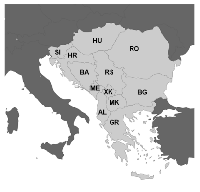
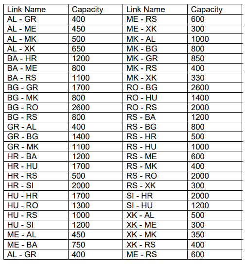
Table 1 shows the installed capacity for each country in SEE while Table 2 shows the capacities for both directions on the NTC-interfaces between the countries.
Table 1. Installed capacities in MW for the six national scenarios

Table 2. NTC-interfaces capacity in MW
The Macedonian power system was modelled with multiple scenarios which differ in the installed capacity of thermal power plants (TPP), hydro power plants (HPP) and VRES. In total, six scenarios were analysed as a combination of conventional power plants (business-asusual (BC), investment in gas (wTPP), and pump-storage HPP (PSP) scenarios (wPSP)) and two VRES development profiles with high and low installed VRES capacity (H-RES and L-RES). Table 3 presents the installed capacity for all six development scenarios for North Macedonia (MK).
Table 3. Installed capacities in MW for the six national scenarios
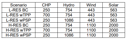
Table 4. Flexibility parameters of the hydro and thermal power plants in MK
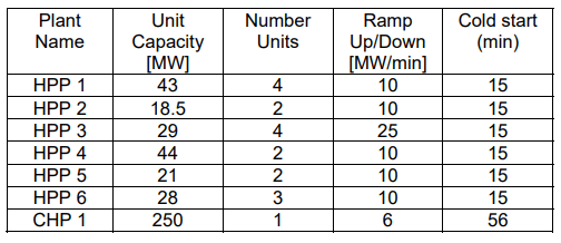
In this paper, for the flexibility analysis of the Macedonian power system, it is considered that only the HPP and gas-fired combined heat and power thermal power plants (CHP) can provide system flexibility. Table 4 presents the flexibility parameters for the Macedonian power system.
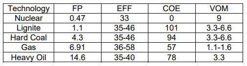
For each TPP in the model the marginal price (MP) was calculated using (1) as:

where VOM are the variable operation and maintenance cost in €/MWh, COE are the TPP CO2 emission rate in kg/Net GJ, FP is the fuel price in €/GJ, EFF is the TPP efficiency in percent, and the coefficient 3.6 is the conversion factor between GJ and MWh. COP is the CO2 price and in this model its value is 66 €/t. The economic parameters used in the market model for the TPPs are given in Table 5, [11].
Table 5. Economic parameters
For all other power plants, the production price is equal to the MP calculated by the simulation tool ANTARES. The Monte Carlo based optimization algorithm is explained in detail in [12]. The Monte Carlo optimization was carried out by simulating 700 Monte Carlo Years as a combination of 35 climatic years (CY) from PECD and 20 random outage patterns of the generators from EMIDB. CY represents a unique combination of the production of wind, solar, hydro and system load on hourly basis based on a historical weather pattern presented in PECD.
The forced outage rate in percent and the forced and planned outage duration in days for different TPPs are given in Table 6.
Table 6. Forced and planned outage rates per TPP fuel type

Flexibility and inertia metrics The assessment of power system flexibility and inertia is quantified by calculating the value of four metrics: RPI, REPI, LORE, and SNSP.
RPI is calculated in two steps as:
Step 1: Calculate RPI using (2) on hourly basis ∀CY as:

where W is the wind production, P is the photovoltaic production, and L is the system load.
Step 2: RPI is equal to the maximum hourly value from all calculated values in Step 1.
REPI is calculated in two steps as:
Step 1: Calculate REPI using (3) on annual basis ∀CY as

Step 2: Calculate REPI using (4) as:

The LORE metric is calculated based on six-step procedure:
Step 1. Calculate the Net Load (NL) ∀CY as:
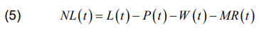
where MR represents all the must-run generation1 in the market simulation.
Step 2. Calculate Net Load Ramp (NLR) ∀CY as:

and split the values calculated with (6) in two subsets, positive or upward net load ramps, NLR+(t), and negative or downward net load ramps, NLR–(t).
Step 3. Calculate the probability for VRES curtailment due to NL value being below zero as:

Step 4. Calculate the probability for VRES curtailment due to NLR+(t) being greater than the ramp-up capability of the Macedonian power system as:

where RU(t) is the remaining ramp-up capability of the power plants in Table 4 based on the dispatch results of the Monte Carlo simulation.
Step 5. Calculate the probability for VRES curtailment due to the absolute value of NLR–(t) being greater than the absolute value of the ramp-down capability of the Macedonian power system as:
where RD(t) is the remaining ramp-down capability of the power plants in Table 4 based on the dispatch results of the Monte Carlo simulation.
Step 6. Calculate LORE based on (8) as:

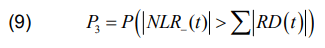
Finally, SNSP is calculated using (9) as:

where E is the exported power from the analysed system on hourly basis. SNSP is calculated for each hour, ∀CS.
From the analysis four metrics were calculated for the Macedonian power system: RPI, REPI, LORE, and SNSP, as described in Section 3.
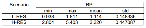
Table 2 and Table 3 show the minimum, maximum, average value, and standard deviation for RPI and REPI, for the L-RES and H-RES scenarios respectively.
Table 7. RPI for the Macedonian power system
1 Must-run generation is all generation that must be dispatched each hour based on the hourly time-series with which the generation technology is modeled.
From Table 2 and Table 3 we can conclude that for both RES development scenarios the distributions are similar and cantered around the mean. The values of Table 3 for the H-RES scenario are in line with the European strategic framework where the mean value of the total production is around 49 % of the total load. Since high RPI values were noted for both L-RES and H-RES, in the future, to avoid VRES production curtailment, the Macedonian strategic framework should be reworked to consider different energy storage technologies or a shift from a fossil fuel-powered industry to an electricity-powered industry to increase the overall load profile [13].
Table 8. REPI for the Macedonian power system

Table 4 shows the loss of renewable energy estimation (LORE) for the six analysed scenarios as well as the results for the three different periods of interest. From the three period only Periods 1 and 2 have a the most significant impact. From the results we can conclude that the commissioning of new TPPs and a PSP is crucial to reduce the curtailment probability. Period 1 contributes the most significantly to LORE in the H-RES scenarios due to the relatively low demand profile. In the future, to lower the probability of RES curtailment storage technologies should be included in the energy and power mix.
Table 9. LORE for the Macedonian power system

It is important to note that the results from the market model did not show curtailment of VRES because of the well-developed interconnections in the region of interest, but at the same time, the installed VRES capacities in the neighbouring countries are quite modest, with exception to the installed capacities in Romania, Greece, and the rapid development VRES scenarios for MK.
Figure 5 shows the SNSP density for the analysed scenarios of the Macedonian power system. In comparison to the L-RES scenario has insignificant effect on system inertia compared to H-RES. In the H-RES scenarios we can note that system inertia get quite low for MK. Since all countries will follow a similar development trend it is expected that all countries in SEE will experience similar or worse trends. Consequently, each country in SEE as well as MK should focus on alternative ways for system inertia provision such as synthetic inertia provision from VRES power plants or subsidization of conventional power plants so they will provide system inertia during hours of high VRES production.
The flexibility analysis for the Macedonian power system was done using a probabilistic market-based calculation on an SEE market model. For MK, six national scenarios were analysed as a combination of three development scenarios for the conventional power plants and two VRES development scenarios. The flexibility was assessed by computing the RPI, REPI, LORE, and SNSP metrics.

The introduction of VRES to the system leads to a high ratio between RPI and REPI as presented in Table 7 and Table 8, which is mainly driven by the low load levels during the periods where the VRES production is highest. Moreover, as shown in Table 9, the LORE parameter increases as more VRES are introduced to the system, which means that the risk for VRES curtailment in the future will be high. Since the flexibility needs are dependent on the regional evolution of the generation profiles in the neighbouring countries, it is expected that as more VRES are introduced, the curtailment risk in MK and the region will be even higher. To alleviate the possibility for VRES curtailment in MK and in SEE each country should focus on further electrification of the energy sector so to increase the base load. Furthermore, each TSO should focus on national and regional flexibility studies so to assess the need for flexibility means such as storage technologies.
The combination of decommissioning of conventional power plants with a rapid introduction of VRES in the generation mix will have detrimental effects on the system inertia as presented on Figure 2. Since the countries in SEE will follow similar trend to the one presented for MK it is expected that system inertia will drop on regional level. To increase system inertia the focus should be on development of national and regional markets so to facilitate synthetic inertia provision from the VRES power plants. Moreover, the feasibility of renumeration mechanisms for inertia provision from conventional power plants should be further explored for periods of high VRES production.
The metrics in this paper are relatively easy to compute, and their computation isn’t computationally intensive compared to other more detailed methods. On the other hand, the market simulations take 24 hour each due to the complexity of the model. The obtained results represent a first-of-a-kind screening of the future flexibility needs in the Macedonian power sector, and they pave the way for future developments in this field on a national level.
Acknowledgement – We express our sincere gratitude to United States Energy Association (USEA) for their unwavering support in the development of this work.
REFERENCES
[1] PwC, MANU, The Strategy for Energy Development of the Republic of North Macedonia until 2040, October 2019.
[2] GIZ, National Energy and Climate Plan of the Republic of North Macedonia, July 2020.
[3] TAF-WB, Programme for the realisation of the Energy Development Strategy 2021 – 2025, March 2021.
[4] Cochran, J & Miller, Mackay & Zinaman, Owen & Milligan, Michael & Arent, Doug & Palmintier, Bryan & O’Malley, Mark & Mueller, S & Lannoye, Eamonn & Tuohy, Aidan & Kujala, B & Sommer, M & Holttinen, Hannele & Kiviluoma, Juha & Soonee, Sushil. (2014). Flexibility in 21st Century Power Systems.
[5] IRENA (2018), Power System Flexibility for the Energy Transition, Part 2: IRENA FlexTool methodology, International Renewable Energy Agency, Abu Dhabi.
[6] IEA (2011), Harnessing Variable Renewables: A Guide to the Balancing Challenge, OECD Publishing, Paris, https://doi.org/10.1787/9789264111394-en.
[7] Dierk Bauknecht, Christoph Heinemann, Moritz Vogel, Study on the impact assessment for a new Directive mainstreaming deployment of renewable energy and ensuring that the EU meets its 2030 renewable energy target, Task 3.1: Historical assessment of progress made since 2005 in integration of renewable electricity in Europe and first-tier indicators for flexibility, July 2019, https://energy.ec.europa.eu/designflexibility-portfolios-member-state-level-facilitate-cost-efficientintegration-high-shares_en
[8] J. Ma, V. Silva, R. Belhomme, D. S. Kirschen and L. F. Ochoa, “Exploring the use of flexibility indices in low carbon power systems,” 2012 3rd IEEE PES Innovative Smart Grid Technologies Europe (ISGT Europe), 2012, pp. 1-5, doi:10.1109/ISGTEurope.2012.6465757.
[9] Poncela Blanco, M., Purvins, A. and Chondrogiannis, S., PanEuropean analysis on power system flexibility, ENERGIES, ISSN 1996-1073, 11 (7), 2018, JRC110658.
[10] ENTSOE, European Resource Adequacy Assessment 2021 Edition – Executive Report, Brussels, 2021, link: https://www.entsoe.eu/outlooks/eraa/eraa-downloads/
[11] USEA, Assessment of the Impact of High Levels of Decarbonization and Clean Energy by 2030 on the Electricity Market and Network Operations in Southeast Europe, 2022
[12] RTEi, Antares Simulator 7.1.0 – OPTIMIZATION PROBLEMS FORMULATION, https://antares-simulator.org
[13] B. Ćosić, G. Krajačić, and N. Duić, “A 100% renewable energy system in the year 2050: The case of Macedonia,” Energy, vol.48, no. 1, pp. 80–87, Dec. 2012, doi:10.1016/j.energy.2012.06.078
Authors: Stojan M. and Sime K. are with the Macedonian Transmission System Operator, department of power system planning, ul. Maksim Gorki no.4, e-mails: stojan.malcheski- @mepso.com.mk and sime.kuzarevski@mepso.com.mk; Jovica V., Jordanco A. and Mirko T. are with the University of st. Cyril and Methodius, Faculty of Electrical Engineering and Information Technology, Rugjer Boshkovikj, e-mails: jovicav@pees-feit.edu.mk, jordanco@pees-feit.edu.mk, and mirko@pees-feit.edu.mk.
Source & Publisher Item Identifier: PRZEGLĄD ELEKTROTECHNICZNY, ISSN 0033-2097, R. 99 NR 6/2023. doi:10.15199/48.2023.06.28
Published by Dranetz Technologies, Inc., Case Study
Distributed Generation (DG) is a method of Demand Response (DR) which is available in select areas of the world. DG has significant implications to both the data center operations and overall profitability. DG is the basic act of relieving the utility grid of desperately needed electrical loads during system economic peaks or emergency situations by utilizing existing stand-by emergency power generators.
By utilizing backup generators to participate in DR programs, Data Center operators are finally able to realize a stream of cash flow for a very expensive investment that otherwise would only be used during low voltage, blackout or utility failure conditions.
Using backup generators has its upside and downside for DG programs, especially in a Data Center or High Tech facility where downtime is lost revenue.
• The upside: Typically backup generators allow for a larger participation value in the DR programs, thus generating more revenue for the company. With proper switching and monitoring equipment, some larger generator system can export power back to the utility grid to gain even more economic benefit. Additionally exercising the generators with load, the transfer switches, and emergency backup procedures ensures that any mechanical issues can be addressed before a “real” emergency happens. Utilizing the Dranetz ES230 family of energy monitors and the Encore Series Software allows companies to verify their energy reductions, generator output, achieved load, and overall benefit to the bottom line and surrounding community.
• The downside: For those facilities with critical or sensitive loads, the act of switching from commercial power to backup power can potentially cause erratic behaviors on computer systems, life safety equipment and general business operations. These impacts can only be realized with adequate Power Quality monitors like the Dranetz 61000 Encore Series, which detail what happens to the electrical system during transitions from commercial to generator and back again. As a result of having this vital data, companies can install and make necessary improvements to limit or eliminate these switching impacts—ideally all of which are paid for by the DG/DR revenues.
Facility operators are separately compensated by the utility, transmission operator, or Independent System Operator (ISO) for their ability to perform load reduction, and typically for their actual performance when called to do so. This revenue can then be utilized to offset or fully pay for maintenance, upgrades, or other energy reduction programs that otherwise would not have been possible. Utilizing the Dranetz ES230 family of energy monitors and the Encore Series Software allows companies to verify their energy reductions, generator output, achieved load, and overall benefit to the bottom line and surrounding community.
Dranetz has supported customers through its power monitoring instrumentation and software in implementing DR programs for many years. The Dranetz Encore System facilitates the measurement and accounting related to demand response, as well as to:
• Implement Energy Reduction and Cost Control Strategies – View and analyze real-time energy demand and usage. Trend and profile that data to shift loads to off-peak hours, improve power factor or reduce consumption.
• Allocate Costs and Perform Activity-based Costing – Track energy-related costs by department, tenant, process or output. Revenue-accurate metering allows for easy cost comparison with utility bills.
• Manage Energy Purchase Agreements – Use historical load profile data to develop price/risk curves for evaluating energy purchase agreements or for joining an aggregated group to purchase power at reduced costs.
• Perform Energy Conservation and Load Reduction – Shed non-essential loads or bring distributed generation on line to reduce consumption and/or participate in utility-sponsored demand reduction programs. Evaluate the value of energy efficient equipment such as lighting and HVAC changes.
• Reduce Demand Peaks and Related Costs – Avoid demand surcharges using the Signature System to predict kW demand and identify the cause of demand peaks and limit peak occurrences. Generate alarms on events such as excessive load, equipment failure, or when operations are likely to exceed contract terms for energy supply.
Source URL: https://www.dranetz.com/technical-support-request/case-studies/data-centers-utilize-distributed-generation/
Dranetz Products: Dranetz HDPQ® Plus & SP Family
Website: Dranetz.com , Call 1-800-372-6832 (US and Canada) or +1-732-287-3680 (International)
Published by Paweł PTAK1, Tomasz PRAUZNER2, Henryk NOGA3, Piotr MIGO3, Agnieszka Gajewska3, Politechnika Częstochowska, Katedra Automatyki, Elektrotechniki i Optoelektroniki (1), Uniwersytet Jana Długosza w Częstochowie, Katedra Pedagogiki (2), Uniwersytet Pedagogiczny w Krakowie, Instytut Nauk Technicznych (3)
Abstract. The paper presents a study on an electromagnetic inductive sensor for detecting and locating faults in protective coatings. The accuracy of the sensor was tested by means of periodic signals of various frequency. A number of measurements were performed for selected signals in order to select required frequencies and to determine the sensitivity and accuracy of the inductive sensor. The possibility of minimising measuring errors was also addressed. Once the frequency and shape of the signal is selected, a multi-frequency binary signal is generated for testing multi-layer anticorrosion coatings. Performing a measurement with a number of different frequencies at a time makes it possible to eliminate sources of errors, such as the necessity to repeat measurements at the same place. The measuring system employs the programming package DasyLab by National Instruments.
Streszczenie. Artykuł prezentuje wyniki badań czujnika elektromagnetycznego indukcyjnego, który będzie w stanie wykryć i zlokalizować wady w badanych powłokach ochronnych. Przedmiotem badań będzie ocena możliwości zastosowania opracowanego inteligentnego systemu pomiarowego na potrzeby przemysłu energetycznego. Sprawdzono dokładność czujnika przy zastosowaniu sygnałów okresowych o różnych kształtach. Dla wybranych rodzajów sygnałów przeprowadzono szereg pomiarów dobierając częstotliwość, określając czułość i dokładność czujnika indukcyjnego oraz oszacowano możliwości zmniejszenia błędów pomiarowych. Dobór częstotliwości i kształtu ma posłużyć zastosowaniu wieloczęstotliwościowych sygnałów binarnych do badania wielowarstwowych powłok antykorozyjnych. Pozwoli to na pomiar wieloma częstotliwościami jednocześnie aby uniknąć szeregu źródeł błędów takich jak powtarzalność miejsca pomiaru. Przedstawiony system pomiarowy wykonano przy zastosowaniu pakietu programowego DasyLab firmy National Instruments. (System pomiarowy do badania stanu powłok ochronnych urządzeń elektroenergetycznych)
Keywords: intelligent measuring system, inductive sensor, modeling, frequency selection, coatings, field measurements of power devices
Słowa kluczowe: inteligentny system pomiarowy, czujnik indukcyjny, badania modelowe, dobór częstotliwości i rodzaju sygnału, powłoki ochronne, pomiary poligonowe konstrukcji energetycznych
A coating is a layer of material created in a natural way or applied on the surface of an object made of a different material in order to obtain desired technological or decorative properties. The coatings applied for both purposes should also meet requirements concerning their appearance, quality, thickness, strength and durability [1,2].
There exists a wide array of devices used for testing the coating parameters, the number of which can be extensive, with individual parameters being tested in a number of ways depending on the standard selected for reference.
Measurements of the thickness of outer layers or coatings are performed in numerous branches of industry, such as automotive, food, electrotechnological, electronic, aviation, metallurgical, computer, telecommunications and plastics industry [3,4,5]. Various types of coatings have to conform to specific standards [6,7,8,9,10].
One of the most widely applied in industry metal coatings is the zinc one. Its durability depends on its thickness and the exploitation conditions. The requirements concerning testing the parameters depend on the production method and also on the function of the element on which the coating has been applied.
Despite the constantly improving quality of anticorrosion coatings, it is corrosion that causes the majority of faults or deterioration of exploitation parameters in devices. Metal elements can be protected from corrosion in a number of ways, one of which is applying zinc, paint, bitumen, or other protective coatings.
Since protective coatings are intended to provide both mechanical strength and electrochemical resistance to corrosion, they consist of a number of layers. Typically, the surface of an element is first covered by a zinc layer and then by a paint layer. Since paint cracks easily, detrimental factors causing corrosion get inside and destroy the layer which is invisible from the outside. Because of that, corrosion is difficult to detect and poses a serious threat to construction elements of the power system. With the internal zinc layer being inaccessible to inspection by means of classical instruments for measuring outer layers, it is necessary to develop alternative nondesctructive methods suitable for this kind of measurement performed during exploitation [1,2,3,4].
The subject of the present study is transformer sensors. The magnetic circuit of the sensor consists of the coating and substrate under scrutiny. The coating is a gap in the circuit. The inductivity of the sensor varies with the gap dimensions and the variation is nonlinear.
The sources of measuring errors in inductive sensors can be classified as:
1. Hardware sources, such as power supply instability, accuracy of the instrument collaborating with the sensor, imprecision of the sensor construction, size of the sensor active surface, supply frequency, size of the surface under examination;
2. Sources related to the object examined and ambient conditions, such as surface roughness, shape of the object, edge effect, temperature, influence of external fields, etc.
Hardware sources of errors can be minimised, but errors related to the object under examination can hardly be eliminated as they are part of the measurement itself. Technological standards stipulate the size of a surface to be tested. However, it is still possible to minimise the influence of such errors to some extent. For example, the influence of the change in the temperature measured in the resistance of the inductive sensor windings can be minimised by applying differential systems. The effect of the surface shape or roughness is minimised by downsizing sensors.
A preliminary selection of the kind of signal and its frequency provides a basis for designing a multi-frequency binary signal (MBS), by means of which it is possible to measure the thickness of a coating and to test the material against delamination (i.e. to test if a third layer has not appeared).
In the laboratory measurements samples of protected car body steel were used, consisting of a steel substrate coated with a layer of zinc and a layer of protective paint. Then, measurements were performed by means of a transformer sensor and compared to the results obtained by means of thickness gauges of known accuracy manufactured by Fisher [13]. Fig. 1 presents the results of the measurements, with accuracy at the level of 1%.
The greatest sensitivity of about 2 mV/µm for a sinusoid measuring signal was attested in the frequency range 11 kHz to 18 kHz. The sensitivity value was calculated on the basis of the measurement data and averaged for that range.
The thickness gauges were also used for measuring the joint thickness of zinc and paint. The accuracy of the measurements was assessed by means of statistical methods, after having performed a number of measurements on previously prepared samples of protective coatings. The accuracy analysis of the measurements performed by the author-designed system were subsequently compared to the data obtained by means of manufactured gauges. The juxtaposition of the results is presented in Fig. 2 [7,8,9,10].

To obtain the value of the standard deviation s, measurements were carried out on two coatings, coating 1 – 120 µm thick and coating 2 – 170 µm thick, with a signal of frequency 1 kHz. 30 measurements were taken for each thickness and for each sensor altogether.
After a series of experiments and analyses, the idea was put forward that the measurements should be performed in two steps:
1. Preliminary measurements intended to recognise the kind of protective coating, select a frequency and create the MBS consisting of 3÷5 frequencies in the range;
2. Measurements proper by means of the MBS.
There are various kinds of instruments for measuring the thickness of multilayer coatings available on the market. One of them is PHASCOPE® PMP10 DUPLEX [13], manufactured by Fischer, used for measuring the thickness of multilayer coatings both on magnetic and non-magnetic substrates [11]. The instrument is not however suitable for measuring the thickness of coatings made of zinc alloys, such as ZnNi or ZnFe, which restricts the range of its applicability.
The intelligent two-phase measuring system under design can be used for measuring the thickness of conductive coatings, such as zinc, together with protective layers on the power system construction or car body elements. The two-phase operation of the device includes recognising a protective coating, selecting a frequency range and forming a MBS consisting of a number of frequencies suitable for the measurement as the first step and the measurement proper by means of the MBS as the second step.
At the preliminary stage of the study, the total thickness of the protective coatings can be measured by means of the inductive method. The thickness of the conducting layer cannot be measured directly since it is located under the external protective non-conducting layer, such as paint. The zinc coating located under the paint layer can be measured by means of an inductive transformer sensor. To verify the usefulness of this method in the first stage of the study, test measurements on zinc coatings 13 µm, 24 µm, 35 µm, 45 µm and 55 µm thick on a 1mm thick ferromagnetic substrate were carried out. The external paint layer was selected in such a way that the joint thickness of both layers, i.e. the zinc one and the paint one was 70 µm. Because of that, the sensor does not respond to variation in the total thickness of the two-layer coating, which is constant, but to the variation in the zinc layer. Fig. 3 presents selected measurement results of the thickness of various zinc coatings.
In the measuring system under design, a transformer sensor will be applied, with a multi-frequency supply signal. When the measuring signal consists of a number of frequencies, it is possible to measure the thickness of conducting and non-conducting layers in a single measurement [6,8].
On the basis of the preliminary results obtained, the intelligent measuring system selected a few component frequencies of the MBS (6 kHz, 8 kHz, 10 kHz and12 kHz) for the case under discussion. For these frequencies, the sensitivity to the changes in the zinc coating thickness was the greatest. The frequencies were selected in such a way as to enable a measurement of a non-ferromagnetic layer, i.e. zinc, by means of two frequencies 6 kHz and 8 kHz. To measure the thickness of the zinc-paint coating on a magnetic substrate, the system selected the frequencies 10 kHz and 12 kHz. The measuring system was modelled by means of the software package DasyLab [12] in two variants, corresponding to two phases of the measurement. In the first variant, presented in Fig. 4, four measuring paths were simulated for a pre-selected frequency of the measuring sensor. Each measuring path corresponds to one frequency of the signal, the amplitude of which can be adjusted. The system computes the maximal value of the signal amplitude for a prescribed number of periods and then determines an average thickness of the zinc coating. On the basis of the results obtained, the component frequencies of the MBS are subsequently determined.

In the second variant, there is only one measuring path (Fig. 5) for the second phase of the measurement carried out by means of a MBS generated in the preliminary phase.

The four modelled signals were combined into one resultant measuring signal. On the basis of its value, the system computes the maximal amplitude, with the prescribed number of signal periods. After these quantities have been determined, the system returns the thickness of the zinc coating.
Applying a few selected frequencies of the sinusoid signal simplifies the measurement by eliminating the need for time-consuming analysis. Because of this, it is possible to apply the method under regular exploitation of the power network, without switching it off. This, in turn, significantly reduces the cost of testing.
Based on the DasyLab package, the measuring system offered in the study enables interactive setting of the measuring signal parameters in response to the varying conditions of the measurement. The standard measuring instruments available on the market, such as Fischer PMP10, are closed systems which do not offer a possibility of modifying their software or the parameters of testing signals.
In both variants of the measuring-diagnostic system it is possible to adjust the amplitude of each component of the MBS, it is also possible to set frequencies different from those obtained in preliminary measurements. The possibility of altering the amplitude is especially useful since with the unmodified value of amplitude, the system can transgress its linear range of operation, thereby increasing the measurement error.
1. The inductive sensor under study can be used for measuring the thickness of protecting coatings as long as it is small with respect to the thickness of a substrate. The measuring signal frequency ranges from 1 to 20 kHz. Due to the fact that the depth of the measuring signal penetration into the coating on a ferromagnetic substrate decreases as the frequency increases, it is necessary to select the signal frequency and amplitude for each surface individually, so as to maximise the measurement accuracy.
2. The measurement method presented in the paper can be used for assessing the corrosion damage of the conducting protective coating, which is inaccessible for testing by means of the instruments based on the classical eddy-current method. The measuring signal can be adjusted to the measuring probe and type of the coating under test. The selection of the measuring frequency in the inductive sensor affects the measurement accuracy.
3. With a multi-frequency signal applied in the sensor, the analysis of the coating condition is more accurate than it would be with a single sinusoid signal. With a multifrequency signal it is possible to measure the thickness of a zinc coating situated under the external protective layer.
The preliminary results of the frequency selection for the measuring signal provide a basis for creating an MBS. The measuring system can be used for observing the operation of an element and diagnosing its parameters in a continuous way. With software based on artificial intelligence, the system will be capable of self-diagnosing. Such system will also adopt itself to the varying conditions of the measurement and requirements of the user.
REFERENCES
[1] Lewińska-Romicka A., Pomiary grubości powłok. Biuro Gamma, Warszawa (2001)
[2] Głowacka M., Inżynieria powierzchni. Powłoki i warstwy wierzchnie – wybrane zagadnienia. Skrypt Politechniki Gdańskiej, Gdańsk (2007)
[3] Ptak P., Borowik L., Diagnostyka zabezpieczeń antykorozyjnych na potrzeby elektroenergetyki. Przegląd Elektrotechniczny, (2012), nr.9a, 142-145
[4] Zloto, T., Ptak, P., Prauzner, T., Analysis of signals from inductive sensors by means of the DasyLab software. Annales UMCS Informatica, (2012), 31-37
[5] May P., Morton D., Zhou E., The design of a ferrite-cored probe. Sensors and Actuators, A 136, 221-228.
[6] Smetana M., Strapacova T., Detection capabilities evaluation of the advanced sensor types in Eddy Current Testing. Przegląd Elektrotechniczny, (2013), nr.3a, 247-249
[7] Ptak P., Janiczek R., Przetworniki indukcyjnościowe w pomiarach grubości warstw wierzchnich. Przegląd Elektrotechniczny, (2007), nr.1, 86- 90
[8] Ptak P., Prauzner T., Badanie czujników detekcji zagrożeń w systemach alarmowych. Przegląd Elektrotechniczny, (2013), nr.10, 274-276
[9] Janiczek R., Ptak P.: Przetworniki indukcyjnościowe w pomiarach grubości warstw wierzchnich. Przegląd Elektrotechniczny, (2007), nr.1, 86- 90
[10] Prauzner T., Finite Element Method in an analysis of selected parameters of an inductive sensor for protective coatings measurements, Przegląd Elektrotechniczny, 91 (2015), nr.12, 205-208
[11] Prauzner T., Interactive computer simulation as a response to contemporary problems of technical education, SOCIETY. INTEGRATION. EDUCATION, Proceedings of the International Scientific Conference. (Vol.II), Rēzekne, (2016), 579-588
Authors: dr Paweł Ptak, Politechnika Częstochowska, Katedra Automatyki, Elektrotechniki i Optoelektroniki, Al. Armii Krajowej 17, 42-200 Częstochowa, e-mail: p.ptak@o2.pl; dr Tomasz Prauzner, Uniwersytet Jana Długosza w Częstochowie, Katedra Pedagogiki, ul. Jerzego Waszyngtona 4/8, 42-200 Częstochowa, e-mail: matompra@poczta.onet.pl; dr hab. Henryk Noga, Uniwersytet Pedagogiczny im. KEN w Krakowie, Instytut Nauk Technicznych, ul. Podchorążych 2, 30-084 Kraków, e-mail: henryk.noga@up.krakow.pl; dr inż. Piotr Migo, Uniwersytet Pedagogiczny im. KEN w Krakowie, Instytut Nauk Technicznych, ul. Podchorążych 2, 30-084 Kraków, e-mail: piotr.migo@up.krakow.pl; mgr Agnieszka Gajewska, Uniwersytet Pedagogiczny im. KEN w Krakowie, Instytut Nauk Technicznych, ul. Podchorążych 2, 30-084 Kraków, e-mail: agnieszka.gajewska@up.krakow.pl
Source & Publisher Item Identifier: PRZEGLĄD ELEKTROTECHNICZNY, ISSN 0033-2097, R. 99 NR 12/2023. doi:10.15199/48.2023.12.65
Published by Dranetz Technologies, Inc., Case Study
Energy and demand costs have a direct impact on a company’s bottom line. In fact, the cost of energy is one of the most commonly mismanaged expenses, regardless of a company’s size or the industry represented. In healthcare facilities energy management can be more difficult than any other industry, because you not only have to manage expenses, but you’re also dealing with managing human lives. Additionally, managing so many different functions within a single operation requires extra work to manage and measure energy improvements. Managing energy expenses does not have to come at a cost of sacrificing patient safety.
A typical facility can save from 10% to as much as 40% annually on energy costs by implementing a comprehensive energy action plan. And, while each facility will require an organized approach to recognize those savings, facilities first need to understand their power consumption, location of major loads, electric demand usage patterns, and associated costs.
A well organized monitoring and reporting system allows determination of where energy is going, identifies the biggest users, and decides which areas are likely to reap the largest benefits from energy management efforts while managing the impacts on patient safety. The benefits from applying monitoring and reporting principles and guidelines can be seen by comparing theoretical, equipment, system, and actual kWh/unit of production as a function of time.
Because a healthcare facility operates so many different areas and operations, the units of production will vary by department. As an example, the Xray, CT, MRI Test Department may be measured on the number of tests performed per hour, day or week vs. the amount of energy consumed; the Emergency Room (ER) would be measured by the number of patients treated per hour; and the Intensive Care Unit would be measured based on the amount of occupied patient beds per hour. Subsequently, in order to realize measurable improvements in energy conservation, it is essential to measure each of the various areas and apply the proper unit of production accordingly.
• Energy expenditure reductions: Load profile can be generated to track daily, weekly and seasonal variations in energy consumption, while critical loads can be metered and sub-metered to evaluate consumption and reduce energy costs.
• Allocate Costs and Perform Activity-based Costing: Track energy-related costs by department, tenant, process or output. Revenue-accurate metering allows for easy cost comparison with utility bills.
• Manage Energy Purchase Agreements: Use historical load profile data to develop price/risk curves for evaluating energy purchase agreements or for joining an aggregated group to purchase power at reduced costs.
• Perform Energy Conservation and Load Reduction: Shed non-essential loads or bring distributed generation on line to reduce consumption and/or participate in utility-sponsored demand reduction programs. Evaluate the value of energy efficient equipment such as lighting and HVAC changes.
• Reduce Demand Peaks and Related Costs: Avoid demand surcharges to predict kW demand and identify the cause of demand peaks and limit peak occurrences. Generate alarms on events such as excessive load, equipment failure, or when operations are likely to exceed contract terms for energy supply.
• Evaluate Impact of Production Equipment on Energy Costs: Monitor the efficiency of large, energy-consuming equipment to improve performance. Plan for expansion by analyzing load trends and available capacity for new equipment.
Source URL: https://www.dranetz.com/technical-support-request/case-studies/energy-management-for-healthcare-facilities/
Dranetz Products: Dranetz HDPQ® Plus & SP Family
Website: Dranetz.com , Call 1-800-372-6832 (US and Canada) or +1-732-287-3680 (International)
