Published by Electrotek Concepts, Inc., PQSoft Case Study: Harmonic Measurement Data Evaluation, Document ID: PQS1001, Date: March 15, 2010.
Abstract: Utility power system harmonic problems can often be solved using a comprehensive approach including site surveys, harmonic measurements, and computer simulations.
This case study presents a harmonic data analysis for a utility 12.47kV substation monitoring location for a two-week period. The analysis included trends of the rms voltage and current and statistical summaries of the voltage and current distortion values. The results of the analysis showed that the harmonic distortion levels were below the IEEE Std. 519 voltage limits.
INTRODUCTION
A harmonic measurement analysis case study was completed for a 12.47kV utility substation bus. The two-week monitoring period was from May 17, 2009 thru June 1, 2009. The power quality instrument used to complete the harmonic measurements was the Dranetz-BMI Encore SeriesTM. The instrument samples voltage at 256 points-per-cycle, current at 128 point-per-cycle, and follows the IEC 61000-4-3 method for characterizing harmonic measurement data. This involves analysis of continuous 200msec samples and storing aggregated 10-minute minimum, average, and maximum trend data. The measurement and statistical analysis was completed using the PQView® program (www.pqview.com).
MEASUREMENT RESULTS
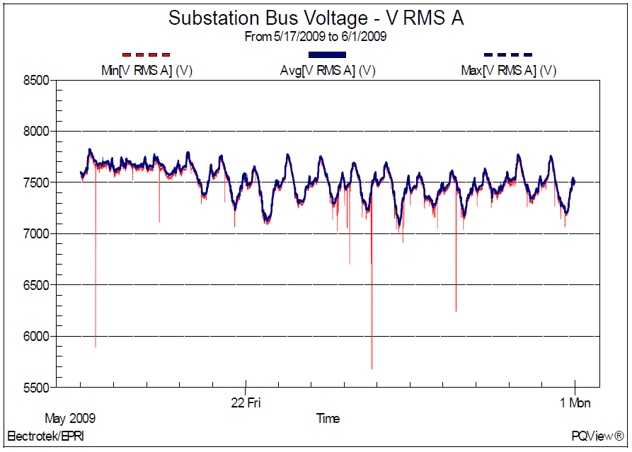
Figure 1 shows the measured rms voltage regulation trend on the 12.47kV substation bus during the two-week period. Various pole-mounted distribution feeder capacitor banks (e.g., 600 kVAr) are switched on-and-off each day using time clock controls in an attempt to maintain a relatively constant voltage. Statistical analysis of the measurement data yields a minimum rms voltage of 12.27kV, an average voltage of 13.02kV, and a maximum voltage of 13.56kV. In addition, the CP95 value was 13.39kV. CP95 refers to the cumulative probability, 95th percentile of a value.
Figure 1 – Measured Substation Bus Voltage Trend
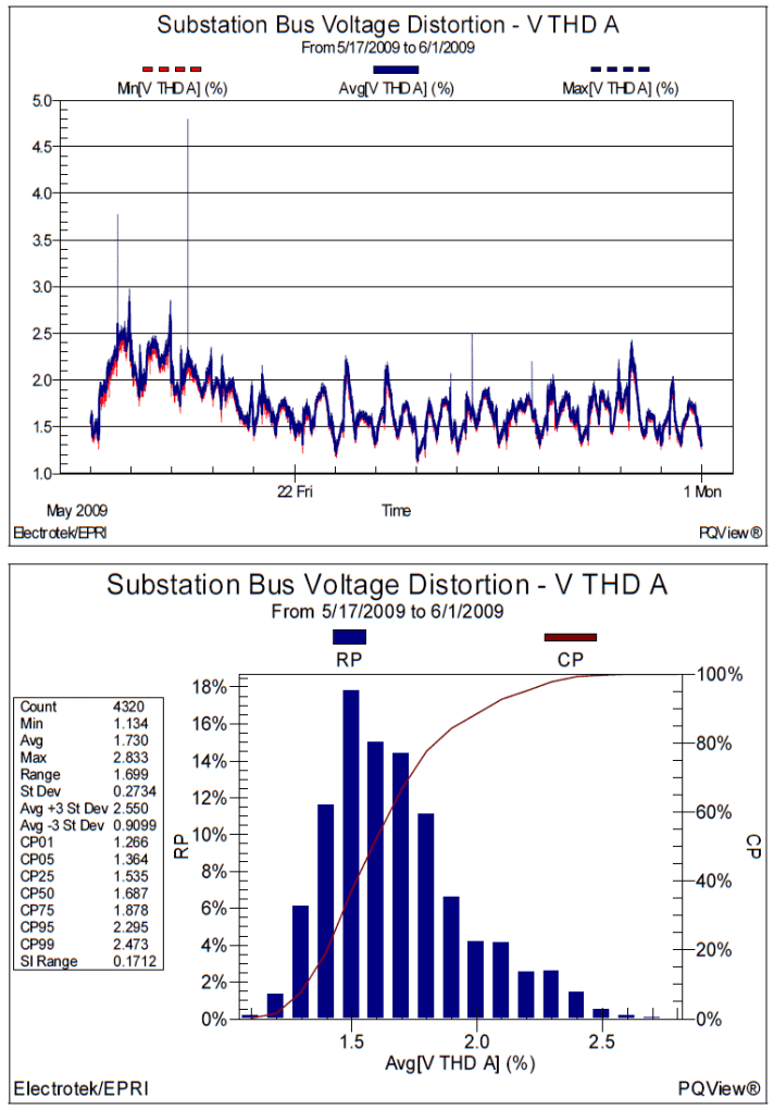
Figure 2 shows the corresponding measured voltage distortion trend and histogram during the two-week period. Statistical analysis of the measurement data yields a minimum distortion of 1.13%, an average distortion of 1.73%, and a maximum distortion 2.83%. The CP95 value was 2.30%.
Figure 2 – Measured Voltage Distortion Trend and Histogram
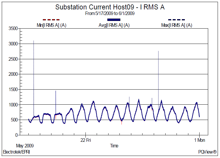
Figure 3 shows the corresponding rms current trend. Statistical analysis yields a minimum current of 378A, an average current of 690A, and a maximum current of 1165A. CP95 value was 1014A.
Figure 3 – Measured Substation Current Trend
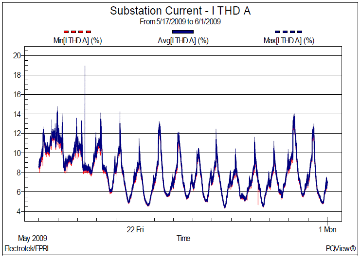
Figure 4 shows the current distortion trend. Statistical analysis yields a minimum distortion of 4.39%, an average distortion of 7.89%, and a maximum distortion 14.24%. CP95 value was 11.73%.
Figure 4 – Measured Current Distortion Trend
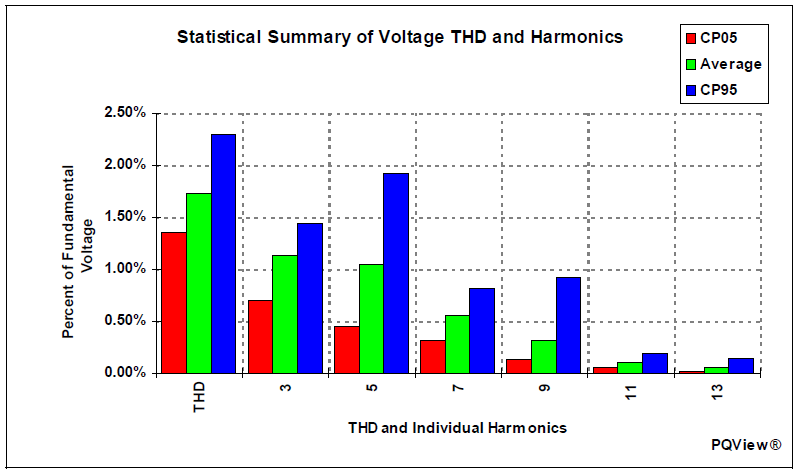
Figure 5 shows the corresponding statistical summary of total harmonic voltage distortion and number of individual harmonics. The analysis shows that the predominate harmonics for the measured substation bus voltages were the 3rd, 5th, 7th, and 9th. The measured values were below the IEEE Std. 519 voltage distortion limits, which are 5% THD and 3% for any individual harmonic.
Figure 5 – Measured Statistical Summary of Voltage Distortion and Harmonics
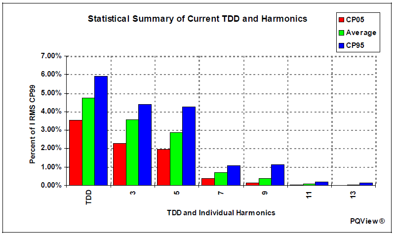
Figure 6 shows the corresponding statistical summary of total harmonic current distortion and number of individual harmonics. The base current for the statistics summary was 1082A.
Figure 6 – Measured Statistical Summary of Current Distortion and Harmonics
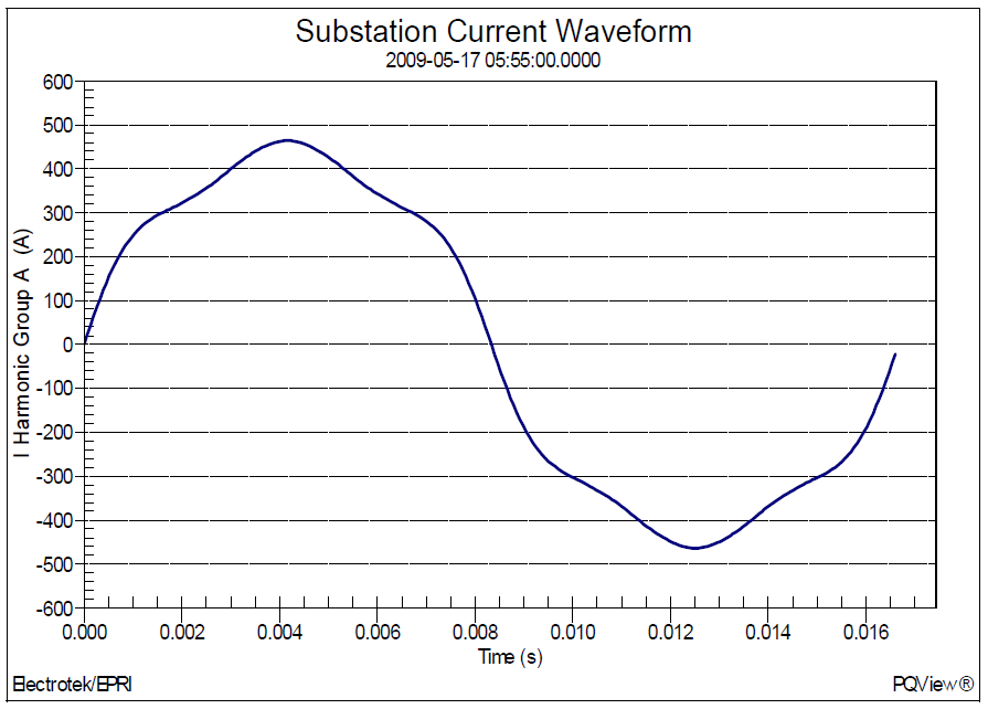
Figure 7 shows one sample calculated harmonic current waveform from the measured harmonic spectrum data. The waveform was created using an inverse DFT with 256 points per cycle. The fundamental frequency current value was 469A, the rms current value was 472A, and the current distortion was 11.8%.
Figure 7 – Example Calculated Substation Current Waveform
SUMMARY
This case study presents a harmonic data analysis for a 12.47kV substation monitoring location for a two-week period. The analysis included trends of the rms voltage and current and statistical summaries of the voltage and current distortion values. The results of the analysis showed that the harmonic distortion levels were below the IEEE Std. 519 voltage limits.
REFERENCES
1. Power System Harmonics, IEEE Tutorial Course, 84 EH0221-2-PWR, 1984. 2. IEEE Recommended Practice for Monitoring Electric Power Quality,” IEEE Std. 1159-1995, IEEE, October 1995, ISBN: 1-55937-549-3. 3. IEEE Recommended Practices and Requirements for Harmonic Control in Electrical Power Systems, IEEE Std. 519-1992, IEEE, ISBN: 1-5593-7239-7.
RELATED STANDARDS IEEE Std. 519-1992 IEEE Std. 1159-1995
GLOSSARY AND ACRONYMS ASD: Adjustable-Speed Drive CF: Crest Factor DPF: Displacement Power Factor PF: Power Factor PWM: Pulse Width Modulation THD: Total Harmonic Distortion TPF: True Power Factor
Published by Bożena MATUSIAK, Anna PAMUŁA, Jerzy S. ZIELIŃSKI, Katedra Informatyki Uniwersytetu Łódzkiego
Abstract. Smart grids and thereafter open grids development implies changes in organizations, technical equipment Power Networks (especially ICT). These new grids influence also on organization and operation of the energy markets, for which it is very important to know correct forecast (mostly short-term) of an electrical energy demand. Excessive requirements concerning accuracy of the forecasting results implied new tools of informatics, especially artificial intelligence application.
Streszczenie. Sieci inteligentne, a potem sieci następnych generacji, spowodują zmiany w organizacji, wyposażeniu technicznym (szczególnie ICT) sieci elektroenergetycznych. Te nowe sieci wpływają także na organizację i działanie rynku energii wymagającego znajomości prawidłowej prognozy (głównie krótkoterminowej) zapotrzebowania na energię elektryczną. Wygórowane wymagania odnośnie do dokładności wyników prognozy spowodowało zastosowanie nowych narzędzi informatyki, głównie sztucznej inteligencji. (Nowa koncepcja rozwoju sieci elektroenergetycznych. Zagadnienia wybrane)
Keywords: smart grids, ICT, energy market, artificial intelligence. Słowa kluczowe: sieci inteligentne, ICT, rynek energii, sztuczna inteligencja.
Introduction
Power Networks development is upon influence of Smart Grid idea. It does not exist one definition of the Smart Grid; in [30] one can find three definitions: from USA, Europe and China. In opinion of the authors the first one is most suitable for this paper and for that reason it will be citation from [30]:
– “It is self-healing (from power disturbance events). – It enables active participation by consumers in demand response. – It operates resiliently against both physical and cyber attacks. – It provides quality power that meets 21st-century needs. – It accommodates all generation and storage options. – It enables new products, services and markets. – It optimizes asset utilization and operating efficiency.”
The above definition of the Smart Grid determines following problems being considered in the paper:
– Basic problems in developing smart grids. – Microgrids. – Selected problems of an energy market in smart grids. – Load- and price forecasting.
Basic problems in developing smart grids [35]
Implementation of the smart grids idea needs new transmission- and distribution grids, large capacity storing devices and number of measurement, monitoring and control devices.
Distribution smart grids additionally must implement Advanced Distribution Management System (ADMS), Advanced Metering Infrastructure (AMI) and Wide Area Monitoring (WAM). All the above mentioned systems imply new problems that are to be solved by Information Communication Technology (ICT).
For example in Germany exist nearly about 3.5·106 measurement points and number of data stored necessary for market information growth 2 TeraBytes/year. It is foreseen generation 22 GigaBytes/day/106 consumers. Storing such number of data is nonsense and data management require data inspection in real time to discover future disturbances.
When consider the smart grids development it is necessary take into account following challenges:
– Dynamic external environment unable exact determination of work completion. – Replacing existing systems with new offering more functionality may be not accepted option from the operational – as well as economical point of view. – Implementation projects are to be accepted by all partners. – Dynamic external environment unable exact determination of work completion. – Replacing existing systems with new offering more functionality may be not accepted option from the operational – as well as economical point of view. – Implementation projects are to be accepted by all partners.
All the above mentioned influence on prediction time of smart grid implementation which seems be far away. Contemporary practice is development step-by step solving separate projects and implementing them.
Microgrids [24]
One of assumptions in smart grids is necessity utilization of Renewable Energy Sources (RES), what implies intrusion in the grid Dispersed Generation (DG) and Dispersed Storage (DS). Operation of the grid with great number of singular DG is difficult and much more easy is to operate a group of DG – Microgrid.
Microgrids it is interconnection of small modular generation to Low- or Medium- voltage distribution systems. Microgrids can be connected to the main power network or be operated islanded, in a coordinated, controlled way [13]
Intrusion of Microgrid into the distribution network (in future smart distribution grid) needs creation of Active Distribution Network (ADN) passing following stages [24]:
– remote monitoring and control of DG and RES, – determination of great number of DG and RES management, – full active power management together with real time communication and remote control.
ADN operation implies necessity of application one of two different strategy: microgrids or virtual consumers. Concept of virtual consumer (virtual energy market) is adaptation of a model similar to information and business ability of Internet. Electrical energy bought from conventional generators, RES or storage devices, according to demand is delivered to agreed nodes. The system would use new ICT technologies as well as advance power electronics and storing devices.
Diversity of RES and storage devices as well as architecture and collaboration with power system implies necessity to define control strategy in operation. “Building Network “ strategy emulate “vacillatory source” in islanded network . DER unit realizing this strategy controls voltage in the connection with the system node setting up the system frequency.
Power and energy management strategy is very important in islanded microgrid and it is more critical than in power system because of specific characteristics of the microgrid.
New ICT needs for an energy market in smart grids
Some countries in Europe such as Italy, UK, Germany and Spain have been largely implemented in the AMI and developed new business processes in the energy market also taking into account the distributed generation and distributed energy sources, including renewable energy. (the results of recent European projects such as EUDEEP, FENIX, MORE MICROGRIDS, SEESGEN-ICT ).
The development of distribution networks in the direction of smart grids in Poland needs investment in infrastructure and ICT tools Some software and existing applications which are already adapted to the new needs of the energy market and intelligent networks in Europe will be summarized as follows in several main groups:
1. Energy flow calculation and market integration tools. 2. Power system analysis tools. 3. Customer portfolio and levels simulation tools. 4. Simulation and optimization tools for DR, DG and energy storage operation. 5. Forecasting and information systems tools. In table 1 there are some ICT samples (you can see and compare: http: //www.dconnolly.net/tools.html)
Table 1. Some samples:
Name of tool
Short Characteristic
Ad 1: Wilmar planning tool
A Strategic planning tool for analyzing the integration of renewable power technologies to be applied by system operators, power producers, potential investors in renewable technologies and energy authorities. The model optimizes power markets based on a description of generation, demand and transmission between defined model regions and derives electricity market prices from marginal system operation costs. The model is a stochastic linear programming model with wind power production as the stochastic input parameter. The model optimizes unit commitment taking into account trading activities of different actors on different energy markets. As a result the simulated output by different production forms, marginal price on each region, and others.
Ad 1: EMPS (multi-area power market simulator
The EMPS model is a stochastic model designed for long-term optimization and simulation of hydro-thermal power system operation. It allows the simulation of large hydro systems with a relatively high degree of detail.. The EMPS model is widely used in the Nordic countries for price forecasting. Large producers can directly employ EMPS in their scheduling decisions. Also thermal plants can be included. The time step is one week and planning horizon is up to several years.
Ad2: Siemens PSSE – Transmission System Analysis and Planning
PSSE is an integrated, interactive program for simulating, analyzing, and optimizing power system performance. It provides the user methods in many technical areas, including: Power Flow, Optimal Power Flow, Balanced or Unbalanced Fault Analysis, Dynamic Simulation, Extended Term Dynamic Simulation, Open Access and Pricing, Transfer Limit Analysis and others
Ad 2: Powerworld Simulator
PowerWorld Simulator is an interactive power systems simulation package designed to simulate high voltage power systems operation on a time frame ranging from several minutes to several days. Potential applications: Transmission Planning, Power Marketing, Simulation of Electricity Markets, Operator Training to improve operators’ knowledge of the system and response to unexpected events, Real-Time System Monitoring, Planning and Operations
Ad3: UPV Flexmod
The tool can calculate the available load reduction and the following payback peak as a function of time when certain load control strategy is used (such as load reduction during morning peak, with allowed temperature drop of 1 °C). The results are specific to certain customer. Each customer is modeled separately.
Ad 3: DER-CAM
DER-CAM ((Distributed Energy Resource Customer Adoption Model) is an economic model of customer DER adoption implemented in the General Algebraic Modeling System (GAMS) optimization software. This model has been in development at Berkeley Lab since 2000. The objective of the model is to minimize the cost of operating on-site generation and combined heat and power (CHP) systems, either for individual customer sites or a micro grid
Ad4: Flexprof
Flexprof has been developed at VTT for assessing the revenues of the aggregation of demand flexibility, integrated with RES in the electricity market. Flexprof tries to simulate trading on the spot market, taking account the possibility of flexibility calls. The situation with and without flexibility can then be compared. It can dynamically allocate the flexibility calls based on market price forecasts. Flexibility allocation is done with linear programming, and the final flexibility calls are obtained with stochastic programming. Any time period can be used in the simulation. One year’s simulation with six customer types takes about one hour. The model has so far been adapted to the English and German market.
Ad4: Offpeak
Offpeak tool can be used for profitability assessment of DER aggregator business. Special attention has been paid to the services that DER can provide within the Great Britain power system. The heuristic-based tool can quickly estimate the profits of several years of operation using historical price data.
Ad5: PrevedoVento
Part of PrevedoEnergia, a tool for forecasting power output from variable renewable energy sources for bidding on power market. PrevedoSole predicts the power output for each PV device according to the provincial solar radiation forecast. The individual outputs are then aggregated for each of seven market zones before bidding as a zonal whole schedule.
Ad5: Inter-Regional Electric Market Model (IREMM)
The IREMM model is based on demand/supply precepts, and is not a “traditional” cost-recovery plus pricing model. IREMM provides a broad-based, comprehensive view of competitive electric power markets: Forecasts market-clearing economy, energy prices, represents all buyers and sellers within an interconnected system simultaneously, identifies economic energy transactions, analyzes the interaction of supply and demand in a competitive bulk power market, is not a cost-based, franchise area-specific pricing model.
Source: on the basis of Seesgen-ICT internal materials: Jussi Ikäheimo VTT (Finland), 2009
Load forecasting
Energy Market operation needs knowledge on demand of electricity and prices in different intervals of time what implies necessity of application of load- and price forecasting tools. Historically the first method applied time series-based methods, but in 20th century the Artificial Intelligence (AI) tools dominate [34]
One of the first well reported application of Expert System (ES) in Short Term Load Forecasting (STLF) is the paper [29] written by S.Rahman and R.Bhatnagar. From that time number of papers presenting application of ES, Artificial Neural Networks (ANN), Fuzzy Logic (FL) and Hybrid Systems (HS) combining no less than one of AI tools with another models is growing. As an illustration of contemporary state of the art we did review papers printed in the three years of the IEEE Trans. on PWRS (2008, 2009, 2010 – Feb) with following results:
– Short-term load forecasting [1,2,3,4,6,19,20,26,29,31] – Forecasting another power system problems: [8,9,11,12,28,33].
Taking into account tools used in these papers we van find: Expert Systems, Artificial Neural Networks, Fuzzy Logic, Wavelet Transform, Models, Statistics, Evolutionary Algorithms, Hybrid Systems. It is worth of mention that dominate application of hybrid system where we can find PSO (Particle Swarm Optimization) Algorithm in Hybrid System with Wavelet transform and Artificial Neural Network [4].
Final Remarks
Smart Grids – new idea in electric power need for designing, construction and operation new tools, devices, services and quite new market integration tools. Not all of them are mature what opens necessity of further researches applying new ICT solutions.
REFERENCES
Abbreviations: PE – IEEE Power & Energy; PWRS – IEEE Trans. on Power Systems
[1] Amjad y N. , Ke yn ia F.: Day-Ahead Price Forecasting of Electricity Markets by Mutual Information Technique and Cascaded Neuro-Evolutionary Algorithm. PWRS, Feb. 09, 306-318. [2] Areekul P., Senjyu T., Toyama H., Yona A.: A Hybrid ARIMA and Neural Network Model for Short-Term Model Price Forecasting in Deregulated Market. PWRS, Jan.10, 524-530. [3] Bas hi r Z.A. , El -Hawar y m.M.E.: Applying Wavelets to Short-Term Load Forecasting Using PSO-Based Neural Networks. PWRS, Feb. 09, 20-27. [4] Bessa R.J. , Miranda V., Gama J. : Applying Wavelets to Short-Term Load Forecasting Using PSO-Based Neural Networks. PWRS, Nov. 09, 1657-1666. [5] Chakrabar t i S., Kyr iakides E., Bi T . , Cai D.: Ter z i ja V.: Measurements Get Together. PE, vol. 7, No.1,4149. [6] Chen Y. , Luh P.B., Guan C., Zhao Y. , Miche l D., Coolbeth M.A. , Friedland P.B., Rourke S.J . : Short- Term Load Forecasting Similar Day-Based Wavelet Neural Networks. PWRS, Feb. 10. 322-330. [7] Dickerman L . , Har r i son J. : A new Car, a New Grid. PE, vol. 8, No. 2, 55-61. [8] Do Couto Fil ho M.B. , Stacchini de Souza J.C: Forecasting-Aided State Estimation – Part I: Panorama. Nov. 09,1667-1677. [9] Do Couto Filho M. B., Stacchini de Souza J .C.: Forecasting-Aided State Estimation – Part II: Implementation. PWRS, Nov. 09,1678-1685. [10] Dr iesen J . , Kat i rei F. : Design for Distributed Energy Resources. PE vol. 7, No. 3, 30-39. [11] El ias C.N., Hatz ia rgyr iou N.D. : An Annual Midterm Energy Forecasting Using Fuzzy Logic. PWRS, Feb. 09, 469-478. [12] Gaj b h iye R.K. , Nai k D. , Dambare S., Soman S. A.: An Expert System Approach for Multi-Year Short-Term Transmission System Planning. An Indian Experience. PWRS, Feb. 08, 226-237. [13] Hat z i argyriou N., Jagoda G., Pamuła A. , Ziel i ński J.S.: Microgr ids. Some Remarks on Polish Experiences in DER Intrusion into Distribution Grids. Large Scale Integration of RES and DG. 25-26 September 2008, Warsaw. [14] Horowi tz S.H., Phadke A.G. , Renz B. A.: The Future of Power Transmission. PE, vol. 8, No.2, 34-40. [15] ICT for a Low Carbon Economy. Smart electricity Distribution Networks. EU Commission, Directoriate-General Information Society and Media: ICT for Sustainable Growth Unit. July 2009. [16] Kat irarei F ., I ravania R., Hatziargyr iou N., Dimeas A. : Microgrids Management, Controls and Operation Aspects of Microgrids. PE, vo. 7, No.3, 54-65. [17] Ki r s chen D. , Bouf fard F. : Keep the Lights On and the Information Flowing. PE, vol. 7, No.1, 55-60. [18] Kroposky B., Lasseter R. , Ise T., Morozumi S., Papathanassiou S. , Hatziargyr iou N. : Making Microgrids Work. PE, vol. 7, No. 3, 41-53. [19] L i vel y M.B. : The Wolf in Pricing, PE, vol. 7, No.1, 61-69. [20] Mao H. , Zeng X. -J. , Leng G., Zhai Y. -J. , Keane J.A. : Short-Term and Mid-term Load Forecasting Using Bilevel Optimisation Model. PWRS, May 09, 1080-1090. [21] Marnay Ch. , Asano H., Papathanassiou S., Strbac G. : Policymaking for Microgrids. Economic and Regulatory Issues of Microgrid Implementation. PE, vol. 7, No. 3, 66-77. [22] Matusiak B. , Pamuła A., Ziel i ński J.S. : Technologiczne i inne bariery dla wdrażania OZE i tworzenia nowych modeli biznesowych na krajowym rynku energii. Rynek Energii nr.4, sierpień 2010, 31-35. [23] Nou rai A. , Kearns D.: Batteries Included. PE, vol.8, No.2, 49- 54. [24] Pamu ła A. , Ziel i ń s k i J .S. : Sterowanie i systemy informatyczne w mikrosieciach.. Rynek Energii, I(III), luty 2009, 63-69. [25] Ph i l ips A. : Staying in Shape. PE vol. 8 No.2, 27-33. [26] Pindoriya N.M., Singh S.N., Singh S.K.: An Adaptive Wavelet Neural Network-Based Energy Price Forecasting in Electricity Market. PWRS, Aug. 08,1423-1432. [27] Piwko R., Mi l ler R., Gi rard R.T.G., MacDowe ll J ., Clar k K. , Murdo ch A. : Generator Fault Tolerance and Grid Codes. PE vol. 8, No. 2, 19-26. [28] Rab iee A. , Shayanfar H.A. , Amjady N.: Reactive Power Pricing. Problems & a Proposal for a Competitive Market. PE, vol.7, No.1, 18-32. [29] Rahman S. , Bh atn agar R.: An expert system based algorithm for short term load forecast. PWRS, vol. 3, No. 2 1988, 392-399. [30] Santacana E., Rackl i f f e G., Tang L. , Feng X.: Getting Smart. PE, vol. 8, No.2, 41-48. [31] Yun Z. , Quan Z., Cai xin S., Shaolan L., Yuming L. , Ya ng S. : RBF Neural Network and ANFIS-Based Short-Term Load Forecasting Approach in Real-Time Price Environment. PWRS, Aug. 08, 853-858. [32] Venkataramanan G., Marnay Ch. : A Larger Role for Microgrids. PE, vo.7, No.3, 78-82. [33] Zhao J.H., Dong Z.Y. , Xu Z ., Wong K.P. : A Statistical Approach for Interval Forecasting of the Electricity Price. PWRS, May 08, 267-276. [34] Ziel i ń s k i J .S. : Artificial Intelligence in power system application. XXX Międzynarodowa Konferencja z Podstaw Elektrotechniki I Teorii Obwodów IC-SPETO 2007, Gliwice- Ustroń 23-26.05.2007, 245-246. [35] Ziel i ń s k i J .S. : Rola teleinformatyki w środowisku sieci inteligentnych. Rynek Energii nr.1, luty 2010, 16-19.
dr Bożena E. Matusiak, Uniwersytet Łódzki, Wydział Zarządzania, Katedra Informatyki. E-mail: bmatusiak@wzmail.uni.lodz.pl; dr Anna Pamuła, Uniwersytet Łódzki, Wydział Zarządzania, Katedra Informatyki, E-mail: apamula@wzmail.uni.lodz.pl. prof. dr hab. Inż. Jerzy S. Zieliński kierownik Katedry Informatyki na Wydziale Zarządzania Uniwersytetu Łódzkiego, uczestnik projektów europejskich: EU DEEP, SYNERGY+, MORE MICROGRIDS, SEESGEN-ICT. E-mail: jzielinski@wzmail.uni.lodz.pl
Source & Publisher Item Identifier: PRZEGLĄD ELEKTROTECHNICZNY (Electrical Review), ISSN 0033-2097, R. 87 NR 2/2011
Published by Tine MARČIČ1, TECES, Research and Development Centre for Electric Machines (1)
Abstract. The paper provides an overview of design problems and contemporary research progress in the currently very interesting field of energy-efficient line-start motors. Discussed are problems related to induction motors (IMs), line-start synchronous reluctance motors and line-start interior permanent magnet synchronous motors (LSIPMSMs). Emphasis is given on small rated power motors, where the LSIPMSM presents the most interesting alternative for replacing IMs widely used in low-cost single-speed drives with ventilator fans, pumps and compressors.
Streszczenie. Artykuł daje przegląd problemów projektowania i postęp we wspólczesnych badaniach w interesującym obszarze wydajności energetycznej silników bezpośredni włączanych. Dyskutowane są problemy związane z silnikami indukcyjnymi, silnikami synchronicznymi reluktancyjnymi z bezpośrednim włączaniem i takie same z magnesem trwałym. Nacisk został położony silniki małej mocy, które skutecznie zastępują silniki indukcyjne w niskokosztowych napędach w wentylatorach, pompach i kompresorach. (Krótki przegląd efektywności energetycznej silników o bezpośrednim włączaniu)
Keywords: computer aided design, induction motors, squirrel cage motors, synchronous motors. Słowa kluczowe: projektowanie wspomagane komputerowo, silniki indukcyjne, silniki klatkowe, silniki synchroniczne
Introduction
Nowadays, a large share of electric energy is converted into useless heat by electric drives worldwide. A large portion of these electric drives is represented by single-speed applications with ventilator fans, pumps and compressors. In such drives the electric motors are mostly started and fed directly from line, i.e. without the usage of any power electronics. Therefore, the used line-starting motors must fulfil one fundamental requirement – they have to be able to start from standstill and accelerate the complete drive to the rated speed when they are fed from a constant amplitude and constant frequency voltage source, i.e. the so called line-starting capability. And considering the elevated environmental conscience and global market trends, the used motors have to exhibit the highest possible efficiency also. However, these two requirements are quite contradictory when the actual motor design is considered. Therefore the line-start motor design process is connected with adequately addressing many design compromises.
This paper is devoted to providing an overview of the contemporary progress from available literature and own research results in the currently very interesting field of energy-efficient line-start motors.
Overview of line-start motor topologies
The line-start brushless motor family includes induction motors (IMs) [1], line-start synchronous reluctance motors (LSSRMs) [2] and line-start interior permanent magnet synchronous motors (LSIPMSMs) [3]. Their principal rotor structures are depicted in Fig. 1, whereas the stator structures are the same [4, 5].
Motor designers utilize different designs of the squirrel-cage (SC) in all previously mentioned line-start motor types. The SC provides asynchronous starting capability or the so called “line-starting capability” and damping of dynamic oscillations at fast load changes also. In relation to IMs (also called asynchronous motors), the SC is usually made of electrically conducting bars which are embedded in slots of the rotor’s iron core and connected on both ends with cage-end rings. In large motors, the SC can be die-casted or fabricated [6] by using different materials. But in large volume production of small rated power motors the SC is mostly die-casted from aluminium and its alloys. The IM performance both in transient- and steady-state heavily depends on the SC and rotor slot design [7].
The SC in rotors of LSSRMs is usually constructed as electrically conducting material within the LSSRM’s magnetic flux barriers (FBs) [2], which are accountable for the main torque producing component of a LSSRM in its steady-state synchronous operating region. Furthermore, the LSIPMSM has permanent magnets (PMs) inserted in FBs, thus different authors have presented many different SC, FB and PM arrangements within rotors of LSIPMSMs [8-27] along with their design methods. The evolution of these rotor designs has been in line with the evolution of PM materials and their contemporary price and availability [28]. However, the one mostly used SC design in LSIPMSMs is still the one similar to IMs and the nowadays mostly used PM material in LSIPMSMs is of Nd-Fe-B type. The PMs and FBs are accountable for the torque producing components of a LSIPMSM in its steady-state synchronous operating region. Due to the hybrid nature of LSSRMs and LSIPMSMs, the motor designer has to account for all the different torque producing components in both the asynchronous and the synchronous operation region.
Fig.1. Principal rotor cross-sections of induction motors (IMs), line-start synchronous reluctance motors (LSSRMs) and line-start interior permanent magnet synchronous motors (LSIPMSMs)
Candidates for energy-efficient line-start motors
IMs have been traditionally used in all kinds of applications, mainly due to their low price and robust construction. However, especially for small rated power IMs, their relatively small efficiency and power factor make them inappropriate for markets with strict regulations regarding energy efficiency. Some previous studies were focused on improving the IM efficiency by using expensive cage materials (copper alloys) also in small-sized IMs [1, 29]. The LSSRMs present an alternative only for larger machines because a large portion of rotor material has to be allocated to FBs in order to achieve sufficient torque capability. Thus, LSIPMSMs with buried PMs bellow the SC are currently identified as the most promising design for energy-efficient small rated power applications [30]. Fig. 2 presents a comparison between the measured characteristics of efficiency and power factor and their product for a 1.1 kW four-pole three-phase LSIPMSM and IM with SCs made from aluminium [3]. The efficiency characteristics can be directly compared to measured characteristics of the same rated power IM with the SC made from copper available in [1]. From that comparison it can be seen that LSIPMSMs offer much higher efficiency increase. But on the other hand, for large machines the efficiency increase of LSIPMSMs in comparison to IMs is far from substantial [5].
Fig.2. Comparison of measured efficiency (EFF) and power factor (PF) characteristics of a 1.1 kW three-phase four-pole LSIPMSM and IM, measured at equal voltage 380 V / 50 Hz
LSIPMSM torque components
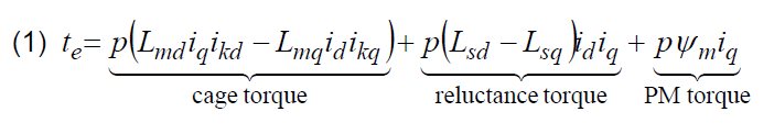
The electromagnetic torque te equation (1) which is part of a LSIPMSM dynamic model written in the d-q reference frame [31] neatly depicts the torque producing components in all line-start motors. In Eq. (1) the subscripts d and q denote variables in the d- and q-axis, respectively; i denotes stator winding currents, ik denotes SC currents, Ls are stator self-inductances, Lm are mutual inductances, Ψm is the length of the PM flux linkage vector, and p is the number of pole pairs.
.
The (asynchronous) cage torque (due to the presence of a SC) influences the LSIPMSM performance in any operation state, where the slip differs from 0. Thus, the cage torque enables line-starting performance and damping of dynamic load oscillations. Apart from the stator winding design, the cage torque depends mainly on the SC design and material.
The synchronous torque components which are represented by the reluctance torque (due to the presence of FBs) and the PM torque (due to the presence of PMs) influence the LSIPMSM performance in any operation state, where the slip differs from 1. In the synchronous operation region (where the slip equals 0) they represent useful torque components. Contrarily, during the line-starting transient they represent braking torques. Thus, they degrade the total torque which should accelerate the LSIPMSM drive up to synchronism. The reluctance torque depends mainly on the design of FBs, which also have to accommodate the used PM segments. The PM torque depends mainly on the placement, dimensions and type of PM material.
For these reasons, the LSIPMSM’s static torque-slip characteristic in the asynchronous operation region is generally lower than the static torque-slip characteristic of a pure IM with the equal SC design, materials, stator and rotor slots geometry and stator winding design. Fig. 3 shows the impact of the aforementioned PM braking torque and the braking reluctance torque on the LSIPMSM’s static torque-slip characteristic [3]. The comparison of measured torque-slip characteristics of a three-phase IM, LSIPMSM and equal LSIPMSM design without PMs in the rotor which actually represents a LSSRM (all with equal SC design) is presented. The difference between the IM torque-slip curve and the LSSRM torque-slip curve at certain slip points represents the reluctance braking torque. And, the difference between the LSSRM torque-slip curve and the LSIPMSM torque-slip curve at certain slip points represents the PM braking torque in the asynchronous operation region.
Fig.3. Measured static torque-slip curves of a three-phase LSIPMSM, equal LSIPMSM design without PMs (i.e. the LSSRM), and IM with equal SC design, at equal voltage
Design process
As it can be noticed from the previous sections, the design problems of LSSRMs and LSIPMSMs are quite similar and are closely related to IM design problems. And usually the main aim of a new LSSRM or a LSIPMSM design is to replace an existing IM, therefore the new motor has to comply with the following two requirements:
– it has to exhibit line-starting and synchronization capability [2, 16, 20, 32];
– in comparison to the existing IM, it has to exhibit a higher (or at least an equal) torque per unit (stator) current density value and a higher efficiency value in its steady-state synchronous operation region [3].
Different authors have used differently complex approaches in coping with design problems [2, 3, 5, 8-27, 32-35]. Strongly coupled finite element (FE) models [5, 21, 23, 33] are in the author’s opinion computationally too complex to be regularly used by motor designers, thus the design procedure depicted in Fig. 4 has been found to be very useful. It has been founded as a hybrid based on preceding knowledge and experience on design, dynamic modelling and analysis of SC IMs [36-39], (cageless) synchronous reluctance motors [40-44] and (cageless) synchronous PM motors [45-49]. The procedure includes employment of the power balance method based on results from time-stepped FE analyses in the analysis of synchronous performance and employment of lumped parameter dynamic models in the analysis of line-starting performance. The power balance method is employed because FE analyses provide a very detailed image of the geometry and material dependant distribution of magnetic field in the machine region. Thus, the FB design, placement and energy-product of PM material, and their effect on iron core saturation and motor parameters are accounted for in sufficient detail. The employed methods and procedures were described and experimentally validated in [3].
Fig.4. LSIPMSMs or LSSRMs design procedure
Design considerations
Along with all the aforementioned, the following list presents further important LSIPMSM design aspects, which should be kept in mind by the motor designers in order to achieve target motor performance where a lot of compromises are to be made [3].
– The motors’ line-starting transient depends on the supply voltage [3, 35] and frequency, the drive inertia [23, 33], the characteristic of the mechanical load, and also the starting position of the rotor [23]. The initial rotor position of the LSIPMSM influences its responding current and speed line-starting transient. Its effect is much expressed when the motor is started without any load.
– The compromise between a LSIPMSM’s adequate line-starting performance in the asynchronous operating region and efficiency in the LSIPMSM’s synchronous operating region is connected to the stator winding’s number of turns. Therefore, the number of turns often has to be adopted in accordance with the target load characteristic, especially when rigorous starting conditions are expected.
– The SC material plays a vital role in the electromechanical performance of line-start motors. A higher cage resistance causes that the motor exhibits a higher starting torque value. But on the other hand, the slope of the torque-slip curve near the synchronous speed is lowered. In relation to IMs, this produces an increase of losses and motor temperature and thus the IM efficiency in steady-state is degraded. However, the impact of SC material on LSSRM and LSIPMSM performance may be more severe. When e.g. a LSIPMSM is line – started, the SC should accelerate the complete LSIPMSM drive up to a certain speed and if the acceleration is sufficient the rotor should be pulled into synchronism. Thus, the LSIPMSM’s “pull-in” transient into synchronism depends on the slope of the static torque – slip characteristic of the LSIPMSM near the synchronous speed, and consequently the LSIPMSM’s starting and synchronization capability depends on the used SC material. Results from different studies which can be related to the cage resistance are available in [23, 26, 34, 35].
Economic considerations
LSIPMSMs with buried PMs bellow the SC are currently identified as the most promising design for energy-efficient small rated power applications. However, motor manufacturers tend to be very rigid when it comes to the manufacture of new motor designs because the manufacturing tools (lamination punching, SC die-casting, winding tools, …) always present a substantial part of the motor manufacturing cost. Therefore, especially in high-volume production of small rated power motors (e.g. ventilator, pump and compressor motors) the manufacturers tend to use existing tools until they are worn out or there is a change on the demand side. Enforcement of stricter policies for motor efficiency (like the EU directive 2005/32/EC) is going to force the manufacturers to consider new motor designs as well.
The manner in which LSIPMSM rotors are manufactured (die-casting of SCs at relatively high temperatures, which are higher than the Curie temperatures of PMs) makes the placement of magnetized magnetic segments in the rotor’s FBs impossible before the SC is die-casted. On the other hand, pulse magnetization of the whole multi-pole rotor with buried PMs presents also a problem, because the induced currents of the SC limit the depth of magnetic field penetration in the rotor area and the magnetization homogeneity of magnetic segments as well [50, 51]. Therefore, the easiest way to manufacture a LSIPMSM rotor is by simple purchase and insertion of pre-magnetized PM segments, which may be quite costly.
An economic assessment and overview of the LSIPMSM manufacturing related cost increase and on the other hand the potential electric energy savings by using LSIPMSMs in contrast to IMs is discussed in [30].
But on the other hand and as indicated before, the motor designers can take advantage of both of the synchronous torque components (i.e. a combination of the PM torque and the reluctance torque as well) where by designing higher rotor saliency, less PM material or cheaper PM material can be used in order to achieve sufficient target synchronous performance.
Conclusion
This work presented an integral overview of the line-start motor design related problems. Discussed and pointed out were LSIPMSM design aspects which were related to IM and LSSRM design as well. These comprise the motors’ construction, stator winding design and the arrangement of SC, PMs and FBs in the rotor; and the manufacturing related economic considerations also.
This work was supported in part by the Slovenian Research Agency, Project No. L2-1180.
REFERENCES
[1] Bogl iet t i A. et al., Energy-efficient motors: Comparing the performance of die-cast copper squirrel cage induction motors with aluminum cage induction motors, IEEE Industrial Electronics Magazine, 2 (2008), No. 4, 32-37 [2] Mi l javec D. et al., Rotor-design and on-line starting-performance analysis of a synchronous-reluctance motor, Compel, 28 (2009), No. 3, 570-582 [3] Mar č i č T. et al., Line-starting three- and single-phase interior permanent magnet synchronous motors—direct comparison to induction motors, IEEE Trans. Magn., 44 (2008), No. 11, 4413-4416 [4] Štumberger G. et al., Comparison of capabilities of reluctance synchronous motor and induction motor, J. Magn. Magn. Mater., 304 (2006), e835-e837 [5] Lu Q. F. , Ye Y. Y. , Design and analysis of large capacity line-start permanent-magnet motor, IEEE Tran. Magn., 44 (2008), No. 11, 4417-4420 [6] Craggs J. L., Fabricated aluminum cage construction in large induction motors, IEEE Trans. Ind. Applicat., IA-12 (1976), No. 3, 261-267 [7] Wi l l iamson S. , McClay C. I. , Optimization of the geometry of closed rotor slots for cage induction motors, IEEE Trans. Ind. Applicat., 32 (1996), No. 3, 560-568 [8] Jovanov ski S. B. , Contribution to the theory of asynchronous performance of synchronous machines with salient poles: Part I, IEEE Tran. Power Ap. Syst., PAS-88 (1969), No. 7, 1150-1161 [9] Jovanovski S. B., Hammam M. S. A. A., Contribution to the theory of asynchronous performance of synchronous machines with salient poles: Part II, IEEE Tran. Power Ap. Syst., PAS-90 (1971), No. 2, 418-426 [10] Honsinger V . B. , Permanent magnet machines: Asychronous operation, IEEE Tran. Power Ap. Syst., PAS-99 (1980), No. 4, 1503-1509 [11] Honsinger V. B., Performance of polyphase permanent magnet machines, IEEE Tran. Power Ap. Syst., PAS-99 (1980), No. 4, 1510-1518 [12] Honsinger V. B., The fields and parameters of interior type AC permanent magnet machines, IEEE Tran. Power Ap. Syst., PAS-101 (1982), No. 4, 867-876 [13] Binns K. J . , Bernard W. R. , Novel design of self-starting synchronous motor, Proceedings of the IEE, 118 (1971), No. 2, 369-372 [14] Binns K. J. et al., Hybrid permanent-magnet synchronous motors, Proceedings of the IEE, 125 (1978), No. 3, 203-208 [15] Binns K. J., Jabbar M. A., High-field self-starting permanent magnet synchronous motor, IEE Proceedings – Electric Power Applications, vol. 128 (1981), No. 3, 157-160 [16] Mi l ler T. J . E. , Synchronization of line-start permanent-magnet AC motors, IEEE Tran. Power Ap. Syst., PAS-103 (1984), No. 7, 1822-1828 [17] Rahman M. A. , Osheiba A. M. , Performance of large line-start permanent magnet synchronous motors, IEEE Tran. Energy Conver., 5 (1990), No. 1, 211-217 [18] Zhou P., Rahman M. A., Jabbar M. A. , Field circuit analysis of permanent magnet synchronous motors, IEEE Tran. Magn., 30 (1994), No. 4, 1350-1359 [19] Rahman M. A. , Zhou P. , Analysis of brushless permanent magnet synchronous motors, IEEE Tran. Ind. Electron., 43 (1996), No. 2, 256-267 [20] Rahman M . A . et al., Synchronization process of line-start permanent magnet synchronous motors, Electr. Mach. Pow. Syst., 25 (1997), No. 6, 577-592 [21] Jabbar M. A., Liu Z., Dong J., Time-stepping finiteelement analysis for the dynamic performance of a permanent magnet synchronous motor, IEEE Tran. Magn., 39 (2003), No.5, 2621-2623 [22] Kurihar a K . et al., Steady-state performance analysis of permanent magnet synchronous motors including space harmonics, IEEE Tran. Magn., 30 (1994), No. 3, 1306-1315 [23] Kur ihara K. , Rahman M. A. , High-efficiency line-start interior permanent-magnet synchronous motors, IEEE Trans. Ind. Appl., 40 (2004), No. 3, 789-796 [24] Abdel-Kader F. M., Osheba S. M., Performance analysis of permanent magnet synchronous motors Part I: Dynamic performance, IEEE Trans. Energy Conver., 5 (1990), No. 2, 366-373 [25] Mi yashi ta K. et al., Development of a high speed 2-pole permanent magnet synchronous motor, IEEE Tran. Power Ap. Syst., PAS-99 (1980), No. 6, 2175-2183 [26] Knight A. M. et al., The design of high-efficiency line-start motors, IEEE Trans. Ind. Appl., 36 (2000), No. 6, 1555-1562 [27] da Silva C. A., Cardoso J. R., Carlson R., Analysis of a three-phase LSPMM by numerical method, IEEE Tran. Magn., 45 (2009), No. 3, 1792-1795 [28]http://www.vacuumschmelze.de/fileadmin/documents/pdf/fipublikationen/2009/NdFeB_Magnets___Properties_and_Applications_revised_13_03_09.pdf {accessed 18th June, 2010} [29] Parasi l i t i F. et al., Three-phase induction motor efficiency improvements with die-cast copper rotor cage and premium steel, Proceedings SPEEDAM 2004, Capri, Italy, pp. 338-343 [30] I s fahani A. H. , Vaez -Zadeh S. , Line start permanent magnet synchronous motors: Challenges and opportunities, Energy, 34 (2009), 1755-1763 [31] Mar č i č T. et al., Determining parameters of a line-start interior permanent magnet synchronous motor model by the differential evolution, IEEE Trans. Magn., 44 (2008), No. 11, 4385-4388 [32] Honsinger V. B . , Inherently stable reluctance motors having improved performance, IEEE Tran. Power Ap. Syst., PAS-91 (1972), No. 4, 1544-1554 [33] Fei W., Luk P. C. K., Ma J . , Shen J. X. , Yang G., A high-performance line-start permanent magnet synchronous motor amended from a small industrial three-phase induction motor, IEEE Tran. Magn., 45 (2009), No. 10, 4724-4727 [34] Ding T. et al., Design and analysis of different line-start PM synchronous motors for oil-pump applications, IEEE Trans. Magn., 45 (2009), No. 3, pp. 1816-1819. [35] Peral ta-Sánchez E. , Smi th A. C. , Line-start permanent-magnet machines using a canned rotor, IEEE Trans. Ind. Appl., 45 (2009), No. 3, 903-910 [36] Dolinar D., Štumberger G., Grčar B. , Calculation of the linear induction motor model parameters using finite elements, IEEE Tran. Magn., 34 (1998), No. 5, 3640-3643 [37] Štefanko S., Slemnik B., Zagradišnik I., Stray losses due to inter-bar currents of skewed cage induction motors at no-load, Electr. Eng., 82 (2000), 257-262 [38] Štumberg e r B . et al., Accuracy of iron loss calculation in electrical machines by using different iron loss models, J. Magn. Magn. Mater., 254-255 (2003), 269-271 [39] Štumberg e r B . et al., Accuracy of iron loss estimation in induction motors by using different iron loss models, J. Magn. Magn. Mater., 272-276 (2004), e1723- e1725 [40] Štumberg e r G . et al., Cross magnetization effect on inductances of linear synchronous reluctance motor under load conditions, IEEE Tran. Magn., 37 (2001), No. 5, 3658-3662 [41] Štumberg e r G . et al., Identification of linear synchronous reluctance motor parameters, IEEE Trans. Ind. Appl., 40 (2004), No. 5, 1317-1324 [42] Štumberger G . et al., Nonlinear model of linear synchronous reluctance motor for real time applications, Compel, 23 (2004), No. 1, 316-327 [43] Štumberg e r G . et al., Evaluation of experimental methods for determining the magnetically nonlinear characteristics of electromagnetic devices, IEEE Tran. Magn., 41 (2005), No. 10, 4030-4032 [44] Štumberger G., Štumberger B., Dolinar D., Dynamic two-axis model of a linear synchronous reluctance motor based on current and position-dependent characteristics of flux linkages, J. Magn. Magn. Mater., 304 (2006), e832-e834 [45] Štumberg e r B . et al., Evaluation of saturation and cross-magnetization effects in interior permanent-magnet synchronous motor, IEEE Trans. Ind. Appl., 39 (2003), No. 5, 1264-1271 [46] Štumberg e r B . et al., Torque ripple reduction in exterior-rotor permanent magnet synchronous motor, J. Magn. Magn. Mater., 304 (2006), e826-e828 [47] Hadžiselimovi ć M. et al., Magnetically nonlinear dynamic model of synchronous motor with permanent magnets, J. Magn. Magn. Mater., 316 (2007), e257-e260 [48] Štumberg e r B . et al., Comparison of torque capability of three-phase permanent magnet synchronous motors with different permanent magnet arrangement, J. Magn. Magn. Mater., 316 (2007), e261-e264 [49] Pišek P., Vi r t i č P. , Štumberger B. , Back EMF and torque characteristic of N-N and N-S type of multi-disc axial flux permanent magnet synchronous generator, Przegląd Elektrotechniczny, 84 (2008), No. 12, 221-223 [50] Lee C. K. et al., Analysis of magnetization of magnet in the rotor of line start permanent magnet motor, IEEE Tran. Magn., 39 (2003), No. 3, 1499-1502 [51] Lee C. K., Kwon B. I., Design of post-assembly magnetization system of line start permanent-magnet motors using FEM, IEEE Tran. Magn., 41 (2005), No. 5, 1928-1931
Author: Dr. Tine Marčič, TECES, Research and Development Centre for Electric Machines, Pobreška cesta 20, SI-2000 Maribor, Slovenia, E-mail: tine.marcic@teces.si.
Source & Publisher Item Identifier: PRZEGLĄD ELEKTROTECHNICZNY (Electrical Review), ISSN 0033-2097, R. 87 NR 3/2011
Published by Dariusz SMUGAŁA(1), Wojciech PIASECKI(1), Magdalena OSTROGÓRSKA(1), Marek FLORKOWSKI(1), Marek FULCZYK(2), Ole GRANHAUG(3), ABB Sp.z.o.o., Corporate Research Center, Cracow, Poland (1), ABB Oy, Medium Voltage Products, Vaasa, Finland (2), ABB AS, Medium Voltage Products, Skien, Norway (3)
Abstract. Novel protection method of wind turbine transformers against high frequency transients occurring during switchgear operation is described in this paper. Presented results are continuation of research on Very Fast Transients mitigation methods previously published in literature [8]. Principles of novel suppressing device parameters optimization for windmill transformers are also included. ATP-EMTP simulations results for wind farm application were verified by full scale functional tests.
Streszczenie. W artykule przedstawiono nową metodę ochrony transformatorów turbin wiatrowych przed wysokoczęstotliwościowymi przepięciami mogącymi wystąpić w trakcie ich pracy. Przedstawione rezultaty są wynikiem kontynuacji wcześniejszych badań prowadzonych nad ochroną transformatorów dystrybucyjnych przed zakłóceniami o wysokokiej częstotliwości mogącymi wystąpić w sieci SN [8, 9]. Wyniki symulacji przepięć oraz doboru parametrów urządzeń ochronnych, zostały zweryfikowane w trakcie testów funkcjonalnych. (Ochrona transformatorów turbin wiatrowych przed przepięciami wysokoczęstotliwościowymi).
Keywords: high frequency transients, transformers, protection, wind turbines Słowa kluczowe: przepięcia wysokoczęstotliwościowe, transformatory rozdzielcze, metody ochrony, turbiny wiatrowe.
Introduction and problem definition
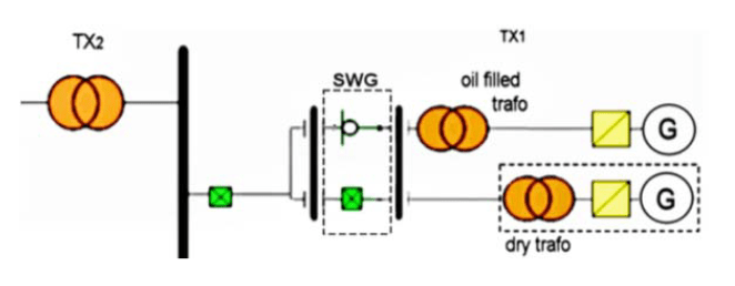
High Frequency (HF) transients influence on wind turbine transformers (especially dry type) has been observed within the research activities presented in this article. They were mainly focused on protection of transformers located at the windmill nacelle. This configuration type is mostly used in practice. Research results presented in this document are study continuation on Fast Transients (FTs) phenomenon overstressing the distribution transformer’s insulation system [2, 4]. Present activities were focused on transients occurrence during normal wind turbine operation [8]. Wind turbines, considering variable operation conditions e.g. wind strength and direction, power network conditions, service, need to be controlled through the breakers operating at relatively high frequency. Presently most of wind turbines, except of air insulated switch-disconnectors, are operated through the Vacuum Circuit Breakers (VCB). Current breaking operations under certain conditions may result in overvoltages generation. During switching operations, interrupters frequently installed into the switchgear (SWG) usually located at the windmill tower bottom, many high frequency transients are generated. In consequence of extremely high voltage steepness (du/dt) occurring e.g. during inductive (e.g. no load) current interruption [3, 5], the insulation system of wind turbine transformers may be overstressed and may lead to pre-mature aging of the insulation material. It may increase transformers failure rate [1, 5, 6]. The high frequency Transient Overvoltages (TOV) problem is dangerous to other connected equipment, e.g. cables and accessories [6]. Generated transients character and overvoltage level depends on wind farm topology and a breaker type. There are two topologies of power network wind turbines connections used in practice (Fig. 1):
– Oil-filled transformer placed at the tower bottom with short connection between the transformer and breaker with long (tens of meters) connection between the transformer and wind turbine with generator,
– Dry-type transformer located at the windmill nacelle with relatively long connection (usually 80÷100 m) with SWG located at the tower bottom.
High frequency transients are generated as a result of relatively short wind turbine cables capacitance (tens of nF, C1,C2 in Fig. 2 and Fig. 3) interaction with low value of dry-type transformer inductance (LT in Fig. 3).
Fig.1. Single wind turbine power network connections topologies
Single windmill power network diagram with dry-type transformer is presented in Fig. 2.
Fig.2. Exemplary wind turbine topology with dry type transformer located at the nacelle (BRK – breaker)
Wind turbine transformer TX1 is connected to the VCB through the cable having capacitance C2. SWG comprising VCB is connected through the cable of C1 capacitance, to the power network connecting point represented by transformer TX2.
Fig.3. Simplified single wind turbine ATP/EMTP power network model: CT, LT – transformer capacitance and inductance, C1, C2 – cable capacitance, LC2 – cable inductance
Additionally, the following factors in MV networks have an influence on the generated transients level:
– switching in/out power network by operating breaker, – ground faults, – pre-strikes and reignitions during switching, – wave reflections if cable surge impedance do not match the transformer impedance.
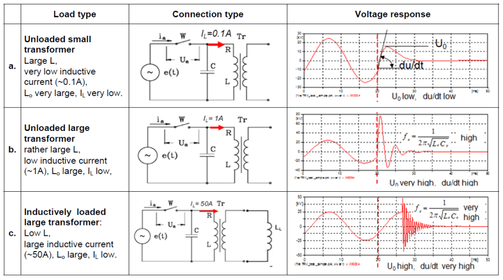
The cable capacitance results in generated transients filtering but simultaneously in interaction with transformer inductance, can be a reason for overvoltages and HF transients. They are in particular related with:
a. Switching-off of an unloaded transformer with high no-load currents values. High natural circuit frequency resulting in fast Transient Recovery Voltage (TRV) build-up, b. Switching-on a transformer to a high-capacitance line. In this case the input capacitance charging from the network capacitance is limited only in practice by the typically very low line resistance.
Moreover, the HF impedance mismatch between the transformer input and the line result in potential wave reflections, multiplying the overvoltage build-up at the transformer terminals.
The effect of reignition level, number of strikes or voltage steepness mainly depends on circuit parameters e.g. cable parameters, but also on circuit breaker type, transformer size and type, supplying voltage level, resonant frequency value etc.
The main problem in avoiding the VFTs is a low value of the surge impedance due to a low impedance of power cables. There are cases described in literature, of the transformer failures during current breaking (e.g. when the VCBs are used for operation [7]). It is supposed that the HF transients occurring during the switching are the most likely the cause for that.
The problem of very high du/dt is enhanced in the case of short connections to the surge source. Increasing the impedance of the surge source may be achieved by introducing a suppressing series element upstream the protected equipment [9].
Solution
There are several transients problem solutions existing in the market and described in the literature [8] e.g. surge capacitors, RC snubbers, series resistors or surge arresters, however all of them have some weak points. Surge arresters protect power network (e.g. transformers) against overvoltages, but does not provide sufficient protection against high voltage steepness occurring during VCB operation. Capacitors and RC snubbers with typical values of this capacitance (C=0.1μF ÷ 0.5μF) are combined with resistance (R=5Ω ÷ 25Ω) and connected upstream the protected device. However they generally provide sufficient protection but they are characterized by large weight, size and significant costs which typically limits its applicability. These features exclude this solution to locate into relatively small windmill tower space. A potentially applicable lowpass RC filter is not acceptable, due to power dissipation and significant voltage drop.
Therefore a special construction of a series impedance element was developed [5]. The device described in [10] consist of series impedance element, coupled with small (≈10nF) capacitance connected upstream the protected device (transformer). At 50/60Hz the impedance of the element is close to zero, at higher frequencies the impedance has a resistive character (close to cable connection impedance). For the windfarm application where cable connection between the breaker and transformer is present, the cable connection capacitance is utilized. Required capacitance is provided by capacitance of power cable (80÷100m) connection between the SWG and transformer.
Taking into consideration high short circuit current rating of SWG, the original air coil construction developed previously, was replaced by high frequency magnetic material.
Suppressing device concept
The limitations of the presently used mitigation methods led to the development of a new concept of high du/dt mitigation using an impedance choke connected in series [6]. Increasing the impedance of the surge source may be achieved by introducing a series, impedance element upstream the protected transformer, as shown in Fig. 4.
Fig.4. Series protective impedance element connected upstream the transformer: C – connection capacitance, Lo – TX2 transformer load inductance
The use of series filter as protecting device is a frequently used method, mostly as common mode chokes in various low voltage systems comprising power electronics.
The choke of appropriately designed frequency characteristic allows significantly increase the voltage wave-front rise time and minimize its influence on the equipment under normal, operating conditions. This means that the choke impedance at 50/60Hz frequency must be close to zero.
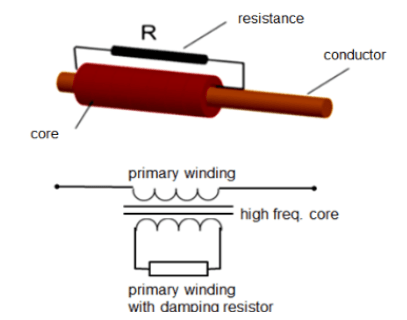
To eliminate risk of destroying protection device as result of short circuit current which may occur into the wind turbine power network, previous protective device was redesigned and improved. Concept based on parallel connection of inductor and resistance was replaced by combination of high frequency magnetic material located at the main conductor e.g. cable, coupled with connected in parallel resistance (Fig.5) .
Fig. 5. Basic diagram of VFTs suppression device solution with cores placed in series and single damping resistor connected in series with secondary winding
The VFTs suppressing device comprises two windings:
– primary winding made of large cross section conductor (e.g. cable placed within), – secondary winding with optimized resistance value.
Inductive impedance can be realized by high permeability magnetic cores put on the main conductor e.g. cable. During normal operation when rated current flows through the conductor and for the short circuit current as well, core are saturated so the inductance is negligible.
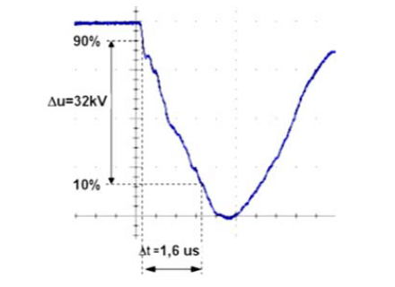
Tab. 1 Dependence of the voltage escalation process during the inductive current disconnection on the current level [8]
.
Suppressing device self-resistance is equal to the main conductor resistance (several μΩ).
For the higher frequencies magnetic rings combination provides required inductance so resistance at the secondary winding provides necessary damping.
To optimize the choke parameters for various magnetic cores and resistance connected in parallel, ATP-EMTP simulations were performed. During analysis various cross-section value cores were simulated having material permeability value near to 30 000. It was experimentally verified that cores characterized by this permeability value provides the best saturation characteristic for most often used in practice wind turbine network topologies. Finally the tested chokes equipped with magnetic components having cross-section from 40 cm2 to 120 cm2 were characterized by summary inductance from 0,6 to 1,5 mH and were tested with transformer connected to the VCB through the specific Zcable cable connection impedance.
The simulations were performed in simplified circuit for the “worst case”. Single re-ignition during VCB operation were treated, for the simulation needs, as voltage step with the magnitude equal the highest system voltage amplitude (in this case 29 kV).
Figures (Fig.6÷Fig.7) presents selected choke current simulation results for various damping resistance values (R1÷R8) and various cores cross-sections. Choke current simultaneously represents choke core saturation occurrence.
Fig.6. Choke current for 40 cm2 core cross-section
The figure below presents the voltage at the transformer when the step voltage is applied for various resistor values.
Fig.7. Voltage at the transformer terminals simulated for 80 cm2 suppressing device core cross-section
Performed simulations indicated that, the best performance is achieved when the resistor value is close to cable wave impedance – Zcable.
Fig.8. Damping resistance value calculation; Voltage at the transformer terminals as a function of choke impedance
Damping resistance should be calculated to provide the best suppressing effectiveness. Voltage at the transformer terminal was taken as the criterion for proper resistance value calculation (Fig.8). Calculation results [8] confirmed the best performance of suppressing device is achieved for resistor value near to cable surge impedance.
The optimal protection provides combination of the choke with additional small capacitor. Especially for the case when the transformer is connected to the circuit-breaker through the short cable characterized by small cable surge impedance.
Functional tests results
New concept of VFT suppressing device functional tests were performed for typical single wind turbine circuit (Fig.1, Fig.2).
Tests stand comprised the following components:
– 630A rated current Ring Main Unit (RMU) equipped with 24 kV VCB, – 3×80 m single phase, 25 mm2 cross-section cable with 33 mH/km inductance and 150 nF/km capacitance – 630 kVA transformer – In Yy 24 kV / 0.24 kV – 3x suppressing devices located between the RMU and transformer (Fig.4)
Tests were performed for various chokes configurations (various resistance and core cross-sections values):
a. base case, no suppression devices, b. 40 cm2, 70 cm2 and 120 cm2 cores cross-section c. Various dumping resistance values from 0.7xZcable to 6xZcable (alternatively no resistor connected) for each version of choke core cross-section
Base case – no active chokes connected In the base case there were no active chokes connected into power network.
Fig.9. Base case, Voltage at R-S-T phases
Fig. 10. Base case, R – phase
Fig.11. Chokes with 70 cm2 core cross-section at T phase and damping resistors R5 at the secondary winding
Fig. 12. Chokes with 40 cm2 cores cross-section and damping resistors R8
Fig.13. Chokes with 40 cm2 cores cross-section and resistors R5 at the secondary winding, phase T
Fig.14. Chokes with 70 cm2 core cross-section in T phase and damping resistors R8
Fig.15. Chokes with 120 cm2 core cross-section at T phase – with resistors R5 at the secondary winding
The experimental results confirmed the applicability of the series-choke protection concept to mitigate high frequency and high du/dt transients.
In cases when the transformer internal capacitance is low, what corresponds to dry-type transformers case, additional small surge capacitor plays an important role in the transients suppression. It has to be pointed out, that the value of the capacitance used was more than an order of magnitude smaller, than typical the value of the typical snubber’s capacitor.
Conclusions
A new mitigation method against high du/dt overvoltage hazards in a form of a series-connected choke element was developed. It was demonstrated that the use of the choke significantly reduces voltage steepness and number of reignitions generated during transformer operated through the breakers. Additionally noticeable overvoltage reduction was observed.
The use of appropriately designed series choke device can:
• Limit the du/dt values at transformer terminals • Limit transient overvoltage • Eliminate wave reflections in cable and HF oscillations (when Zchoke = Zcable) • Eliminate or reduce the number of re-ignitions (requires C in order to lower oscillation frequency
The problem of potential VFT-related hazard to transformer and other power equipment resulted from switching operations was demonstrated in a practical case. The number of pre-strikes during contact making was reduced and high frequency oscillations were practically eliminated.
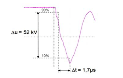
High du/dt was over 2x reduced with the use of the chokes only. Further reduction was achieved when a small (10nF) surge capacitors were used. Prototypes of chokes were experimentally tested and confirmed the applicability of the series-choke protection concept to mitigating high du/dt transients resulting e.g. from the VCB switching operations. The resistor value should provide the best suppressing effectiveness. The voltage at the transformer terminal was taken as the criterion. Simulation results demonstrated that the best performance of suppressing device is achieved for resistor value close to cable surge impedance The parameters of the recorded during the tests transients were presented in Tab. 2 and Fig 16.
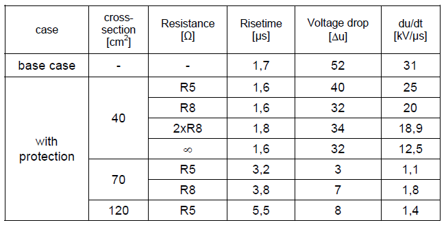
Tab. 2. Average du/dt values observed during tests
.
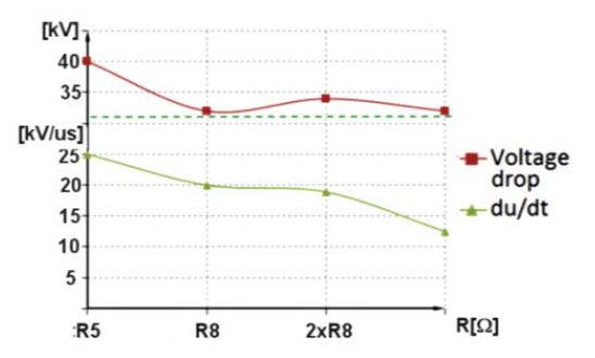
Fig.16. VFTs parameters for 40cm2 core cross-section and various damping resistance values
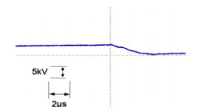
When chokes are inactive and no suppressing device is connected before transformer voltage steepness is few tens of kilovolts per microsecond.
Connecting chokes with larger core cross-section, results both in the voltage steepness reduction and the overvoltage peaks suppression. For relatively large permeability cores with cross-section (40 cm2), du/dt reduction is insignificant then for cross-section larger (70 ÷ 120 cm2) du/dt reduction is very high (up to 10x).
For all tested chokes high degree of oscillation reduction is observed during breaking, especially when additional suppressing resistor is connected at the secondary winding.
Performed experiments demonstrated that, despite that the risetimes of the waveforms observed at the transformer terminals for the base case (with no protection) were relatively long due to the experiment set-up limitations, a significant reduction in the transients amplitudes was observed. Especially, when an appropriate combination of core parameters and the resistance value was applied.
REFERENCES
[1] CIGRE working group A2-A3-B3.21, Electrical Environment of Transformers; Impact of fast transients”, ELECTRA 208, (2005) [2] Lopez–Roldan J., De Herdt H., Min J., Van Velthove R., Decklerq J., Sels T., Karas J., Van Dommelen D., Popow P., Van der Sluis L., Aquado M., Study of interaction between distribution transformer and vacuum circuit breaker, Proceedings of 13th ISH (2003), pp. 62÷64 [3] Popov M., Acha E., Overvoltages due to switching off an unloaded transformer with a vacuum circuit breaker, IEEE Trans. on Power Delivery, Vol. 14, No. 4, (1999), pp. 1317÷1322 [4] Burrage L. M., Shaw J. H., McConnell B. W., Distribution transformer performance when subjected to steep front impulses, IEEE Trans. on Power Delivery, Vol. 5, No. 2, (1990) [5] Piasecki W., Bywalec G., Florkowski M., Fulczyk M., Furgal J., New approach towards Very Fast Transients suppression, Proceedings of IPST’2007 [6] Paul D., Failure Analysis of Dry-Type Power Transformer, IEEE Transaction on Industry Applications, Vol. 37, No. 3, (2001) [7] Wong S. M., Snider L. A., Lo E. W. C., Overvoltages and reignition behavior of vacuum circuit breaker, Proceedings of IPST’2003 [8] Smugała D., Piasecki W. , Ostrogórska M., Florkowski M., Fulczyk M., Kłys P., Distribution transformers protection against High Frequency Switching Transients, PRZEGLĄD ELEKTROTECHNICZNY (Electrical Review), ISSN 0033-2097, R. 88 NR 5a/2012 [9] Florkowski M.,Fulczyk M.,Ostrogórska M., Piasecki W., Steepness reduction of ultra-fast chopped surges at transformer terminal, ICHVE (2012), pp.145÷149
Authors/Autorzy: Dariusz Smugała, PhD. Eng., E-mail: dariusz.smugala@pl.abb.com Magdalena Ostrogórska, MsC.Eng. E-mail: magdalena.ostrogorska@pl.abb.com Wojciech Piasecki, PhD.Eng., E-mail: wojciech.piasecki@pl.abb.com Marek Florkowski, PhD,DSc.,Eng E-mail: marek.florkowski@pl.abb.com ABB Corporate Research Center, Starowislna 13 A Str., 31-038 Cracow, Poland, Marek Fulczyk, PhD.Eng. E-mail: marek.fulczyk@pl.abb.com Muottitie 2, 65100 Vaasa, Finland Ole Granhaug, MSc.Eng. E-mail: ole.granhaug@no.abb.com ABB AS Amtm. Aallsgate 73, P.O. Box 108 Sentrum, 3717, Norway
Source & Publisher Item Identifier: PRZEGLĄD ELEKTROTECHNICZNY, ISSN 0033-2097, R. 89 NR 10/2013
Published by Blagoja MARKOVSKI, Leonid GRCEV, Vesna ARNAUTOVSKI-TOSEVA, Marija KACARSKA, Ss. Cyril and Methodius University of Skopje, Faculty of Electrical Engineering and Information Technologies
Abstract. We analyze the transient grounding characteristics of interconnected wind turbine grounding systems, for fast rising current pulses. By increasing the number of wind turbines, influences on harmonic impedance and transient potential are examined for different soil characteristics and different locations of excitation. Simulations are performed using simple model of grounding system that neglects the foundation reinforcement. The influence of such simplification for isolated wind turbines is analyzed in previous papers. Here we extend the previous analysis for interconnected wind turbines and we look at the possibilities for optimization of the transient analysis of extended grounding systems in wind farms.
Streszczenie. Przeanalizowano w pracy charakterystyki stanów przejściowych uziemień turbin wiatrowych dla szybkiego narastania impulsów prądowych. Przy wzroście liczby turbin wiatrowych zbadano wpływu na impedancje harmoniczną oraz stan przejściowy dla różnych charakterystyk gleby i różnych lokalizacji wzbudzenia. Przeprowadzono symulacje przy użycie prostego modelu uziemienia, który zaniedbuje wzmocnienie fundamentów. Wpływ takiego uproszczenia dla pojedynczych turbin przebadany został w e wcześniejszych publikacjach. W tym artykule rozszerzono poprzednia analizę na połączone turbiny oraz skierowano uwagę na możliwości optymalizacji analizy stanów przejściowych rozbudowanych systemów uziemienia na farmach wiatrowych. (Wyznaczenie stanu przejściowego w systemie uziemienia elektrowni wiatrowej ).
Keywords: grounding system, lightning, transient analysis, wind turbine. Słowa kluczowe: systemy uziemienia, wyładowania atmosferyczne, analiza stanu przejściowego, turbina wiatrowa
Introduction
Recently a number of papers have been devoted to the transient performance of isolated wind turbine grounding systems [1-4]. In practice, wind turbines are often spread across large areas, electrically interconnected by buried medium voltage cables. Metallic armour of such cables and bare wires are bonded to the wind turbine grounding electrodes, forming an extended grounding system. Such connection should provide significant reduction of the overall grounding resistance [5]. Due to the specific construction at exposed locations, wind turbines often suffer direct lightning strikes that may provoke damage or malfunction on the equipment. Therefore the high frequency performance of interconnected grounding systems is of great practical interest.
In this paper we analyze the transient performance of extended grounding system in wind farm. We consider typical grounding systems of wind turbines with spread footing foundations, interconnected with bare wires buried at depth of 0.5 m. Mutual separation between wind turbines will be varied between 75 m and 300 m to analyze the influence of the length of the buried bare conductor that is in direct contact with earth (only in case of three wind turbines in row, in other cases mutual separation is 300 m ). Details of the grounding system geometry are given in Fig. 1. By increasing the number of wind turbines, influences on the harmonic impedance and on the transient potential will be examined for different types of soil and for lightning current pulses related to the first and subsequent return strokes.
Wind turbine arrangement is illustrated in Fig. 2. Two cases of lightning strike, one in the middle and at the end of the row are analyzed separately. Simulations are performed using simplified model of wind turbine grounding system that neglects the foundation reinforcement mesh.
Recent papers have shown that simplified models for isolated wind turbine grounding system lead to significant overestimation of the transient potential and harmonic impedance in the high frequency range [6-7]. Here we extend the previous analysis for interconnected grounding systems. We compare the influence on the harmonic impedance and transient potential for simplified model of the adjacent grounding system and for model that integrates the foundation reinforcement (see Fig. 1).
Rigorous electromagnetic model is used for the computations [8–9], based on a mathematical method developed from the antenna theory and solved by the method of moments. This model is implemented into the Tragsys computer software [10].
Fig.1. Wind turbine grounding system (thick lines) integrated with the foundation reinforcement mesh (thin lines)
Fig.2. Illustration of wind turbines arrangement
Frequency domain analysis
Harmonic impedance is important quantity in transient analysis of grounding systems. It does not depend on the excitation, but solely on geometry and electromagnetic characteristics of the grounding system and surrounding medium. It is equal to the grounding resistance R in the low frequency range and it has larger or smaller values than R in the high frequency range, whether the inductive or capacitive characteristics of the system are dominant.
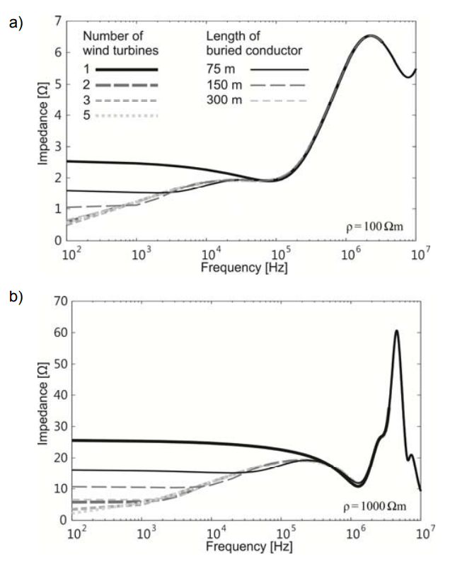
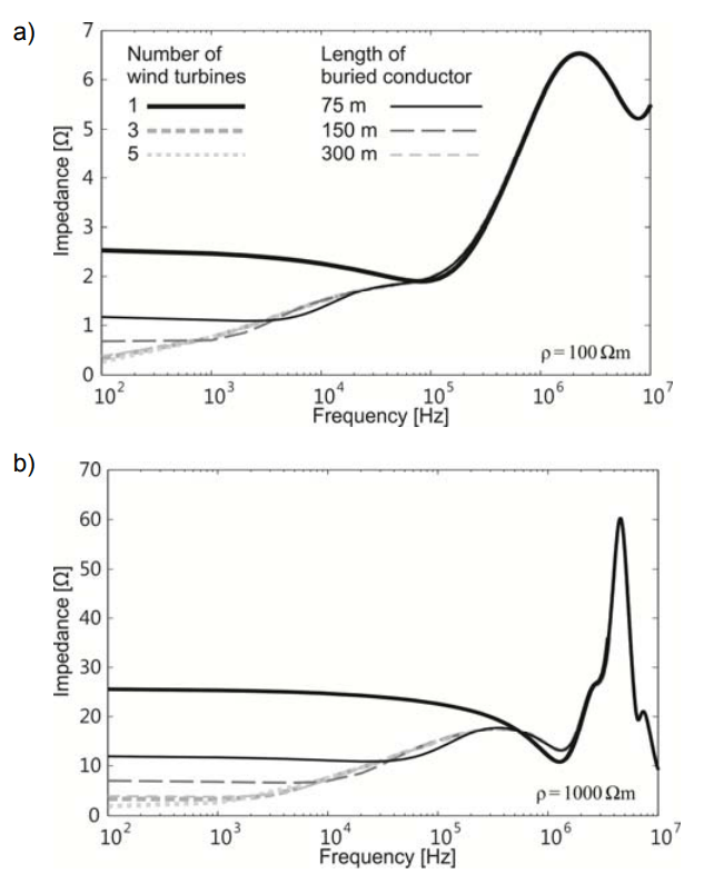
Current with variable frequency from 100 Hz to 10 MHz is injected in the vertical conductors above earth, in one grounding system of the row (see Fig.2). Analysis are performed for low resistive earth, with ρ = 100 Ωm, and highly resistive earth, with ρ = 1000 Ωm, for excitation in the middle and at the end of the row. We analyze the influence of the buried bare bonding wires and the influence of the adjacent grounding systems. The foundation reinforcement mesh is omitted due to computational efficiency and its influence will be analyzed later.
From Fig. 3 and Fig. 4, it is evident that the buried horizontal bare wires have major influence on the reduction of the harmonic impedance in the low frequency range, while the influence of the adjacent grounding systems is considerably lower. The interconnection of several wind turbines improves the grounding performance for slow varying excitations with low frequency contents, such as fault currents or slow rising current pulses (typical for first lightning strokes) in case of highly resistive earth. However due to the great mutual separations, the adjacent grounding systems do not provide improvement in case of fast rising lightning current pulses (typical for subsequent return strokes). At high frequencies, currents dissipate only locally, near the affected wind turbine grounding system.
Time domain analysis in case of lightning strike
Time domain analysis are important for proper design of protective equipment. We analyze the transient potential (in respect to distant neutral earth) at current feed points, for low resistive earth with ρ = 100 Ωm and for highly resistive earth with ρ = 1000 Ωm. Two standardized lightning current waveforms related to the first and subsequent return strokes are considered. They are reproduced by means of a usual double exponential function:
.
where Im is the peak value of the current pulse. Values of the coefficients k, τ1 and τ2 for the current pulses are given in Table 1
Table 1. Parameters of first and subsequent lightning current pulse
T1/T2 [μs]
Im [kA]
k
τ1 [μs]
τ2 [μs]
10/350
200
0.951
0.00211
0.2485
0.25/100
50
0.995
0.00699
10.87
.
Fig.5 illustrates the transient potential at current feed points, for lightning current pulse related to the subsequent return stoke, injected in grounding system at the end of the row. Wind turbine interconnection has no influence on the transient potential in the initial surge period, during the current pulse rise, while the horizontal buried bare conductors significantly reduce the transient potential during the pulse decay. The adjacent grounding systems contribute to further reduction only in case of highly resistive earth, after a period of the decay time to half-peak. In case of low resistivity earth the adjacent grounding systems and the horizontal conductors longer than 200 m do not provide improvement of the transient performance
Fig.3. Harmonic impedance of interconnected wind turbines, for excitation at the end of the row: a) ρ=100 Ωm; b) ρ=1000 Ωm.
Fig.4. Harmonic impedance of interconnected wind turbines, for excitation at the middle of the row: a) ρ=100 Ωm; b) ρ=1000 Ωm.
Fig.5. Transient potential in respect to distant neutral earth for current pulse related to subsequent return stroke in low and highly resistive earth: a) ρ=100 Ωm; b) ρ=1000 Ωm.
Fig.6. Transient potential in respect to distant neutral earth for current pulse related to first stroke in low and highly resistive earth: a) ρ=100 Ωm; b) ρ=1000 Ωm.
Fig.6 illustrates the transient potential at current feed points, for lightning current pulse related to the first stoke, injected in grounding system at the end of the row. Transient response in case of slow rising current pulse is primarily governed by the low frequency behaviour of the harmonic impedance. In case of low resistive earth, the adjacent grounding systems provide small reduction of the transient potential during the entire transient period, while the main contribution comes from the buried bare bonding wires. In case of highly resistive earth, adjacent grounding systems provide significant reduction of the transient potential, after a period of the decay time to half-peak.
It is worth noting that for excitations in the middle of the row, harmonic impedance has lower values in the low frequency range (relative to the earth resistivity) than for excitations at the end of the row. Consequently, transient potentials are expected to be considerably reduced for first lightning stroke, and during the pulse decay for subsequent return strokes
Influence of the grounding system models in transient analysis of extended grounding systems in wind farms
Previous analysis have been performed using simplified model of grounding system that neglects the influence of the foundation reinforcement mesh, (see Fig. 1, with thin lines). Such model leads to significant overestimation of the transient potential, since the foundation reinforcement mesh provides additional paths of the lightning current and reduces the inductive behaviour of the harmonic impedance in the high frequency range. To analyze the influence of the grounding system models, we compare three cases. First the excited and the adjacent grounding systems are modelled by simple geometry that includes only the basic grounding electrodes. Next we use complex model for the adjacent grounding system, integrated with the foundation reinforcement. Finally we use complex integrated models for the two interconnected grounding systems.
Fig.7 shows that the complexity of the model for adjacent grounding system has no influence on the low frequency and high frequency performance of the grounding systems. The use of complex model that integrates the foundation reinforcement mesh has significance only for the local wind turbine grounding system, in case of transient analysis for fast rising current pulses. For low frequency analysis the use of simplified model for the local grounding system will not introduce significant errors.
Fig.7. Influence of the model for local and adjacent grounding systems: a) ρ=100 Ωm; b) ρ=1000 Ωm
Conclusion
When wind turbine grounding systems are interconnected by buried bare wires, these wires are most effective in the improvement of the transient performance. Adjacent grounding systems provide negligible improvement of the transient performance in case of low resistive earth. For highly resistive earth, the adjacent grounding systems provide additional improvement of the transient performance, during the pulse decay period that is mostly governed by the low frequency behaviour of the extended grounding system.
The analysis for lightning strikes at the end of the cascade can be considered as worst case analysis for interconnected grounding systems. Lightning strikes to wind turbines in the middle of the row will produce lower transient potentials. This is due to the lower values of the harmonic impedance in the low frequency range for different types of soil (see Fig.4), than in case of excitation at the end of the row (see Fig.3).
The use of complex model of grounding system, integrated with the dense mesh of the foundation reinforcement has significance only for the local grounding system that is directly affected by the lightning current pulse. For low frequency analysis, simple model of grounding system can be used as well. The complexity of the adjacent grounding systems has negligible influence on the transient performance of the extended grounding system. This observation is important for optimization and reduction of the computational times during transient analysis of extended grounding systems
REFERENCES
[1] Y. Yoh, Y. Takuma, FDTD analysis of wind turbine earthning, in Proc. 28-th Int. Conf. Lightning Protection, (2006), 1551- 1556. [2] S. Pastromas, E. Pyrgioti, Two types of earthning system of lightning protection for wind turbines, in Proc. 29th Int. Conf. on Lightning Protection, (2008), 1-10. [3] A. Elmghairbi, A. Haddad, H. Griffiths, Potential rise and safety voltages of wind turbine earthning systems under transient conditions, in Proc. 20th Int. Conf. Electricity Distribution (CIRED 2009), (2009), 1-4. [4] S. Yanagawa, D. Natsuno, K. Yamamoto, Measurements of transient grounding characteristics of a MW class wind turbine generator system and its considerations, in Proc. 31st Int. Conf. on Lightning Protection, (2012), 1-5. [5] Wind Turbine Generator Systems – Part 24: Lightning protection, IEC Std. 61400-24, (2010). [6] B. Markovski, L. Grcev, V. Arnautovski-Toseva, Step and touch voltages near wind turbine grounding during lightning strokes, International Symposium on Electromagnetic Compatibility (EMC Europe 2012), (2012), 1-6. [7] B. Markovski, L. Grcev, V. Arnautovski-Toseva, Transient characteristics of wind turbine grounding, Frequency dependent and soil ionization effects, in Proc. 31st Int. Conf. on Lightning Protection, (2012), 1-6. [8] L. Grcev and F. Dawalibi, An electromagnetic model for transients in grounding system, IEEE Trans. Power Delivery, 5 (1990), 1773-1781. [9] L. Grcev, Computer analysis of transient voltages in large grounding systems, IEEE Trans. Power Delivery, 11 (1996), 815-823. [10] TRAGSYS-software for high frequency and transient analysis of grounding systems. http://www.tragsys.com
Authors: M.Sc. Blagoja Markovski, Ss. Cyril and Methodius University, Faculty of Electrical Engineering and Information Technologies, P.O. Box 574, 1000 Skopje, Macedonia, Email: bmarkovski@feit.ukim.edu.mk; Prof. Dr. Leonid Grcev, Ss. Cyril and Methodius University, Faculty of Electrical Engineering and Information Technologies, P.O. Box 574, 1000 Skopje, Macedonia, Email: lgrcev@feit.ukim.edu.mk; Prof. Dr. Vesna Arnautovski-Toseva, Ss. Cyril and Methodius University, Faculty of Electrical Engineering and Information Technologies, P.O. Box 574, 1000 Skopje, Macedonia, Email: atvesna@feit.ukim.edu.mk; Prof. Dr. Marija Kacarska, Ss. Cyril and Methodius University, Faculty of Electrical Engineering and Information Technologies, P.O. Box 574, 1000 Skopje, Macedonia, Email: mkacar@feit.ukim.edu.mk
Source & Publisher Item Identifier: PRZEGLĄD ELEKTROTECHNICZNY, ISSN 0033-2097, R. 91 NR 6/2015. doi:10.15199/48.2015.06.13
Published by Electrotek Concepts, Inc., PQSoft Case Study: Harmonic Current Cancellation Evaluation, Document ID: PQS1002, Date: March 15, 2010.
Abstract: Utility power system harmonic problems can often be solved using a comprehensive approach including site surveys, harmonic measurements, and computer simulations.
This case study presents the results for a customer step-down transformer harmonic current cancellation evaluation. The analysis was completed using the SuperHarm program. The simulation results show the reduction of the customer primary harmonic current distortion level due to the phase shifting caused by the different step-down transformer connections.
INTRODUCTION
A harmonic current cancellation evaluation was completed for the system shown in Figure 1. The case study was completed using the SuperHarm program. The accuracy of the simulation model was verified using three-phase and single-line-to-ground fault currents and other steady-state quantities.
Isolation transformers can be used with multiple nonlinear loads to create an effective twelve-pulse operation. In an actual twelve-pulse configuration, the front-end rectifier circuit uses twelve diodes instead of six. When properly designed, this configuration practically eliminates the 5th and 7th harmonics. The disadvantages of this design are cost and construction due to the requirement for either a delta-delta/delta-wye transformer pair, or a three-winding transformer to accomplish the 30° phase shifting necessary for proper operation. This configuration also affects the overall drive system efficiency rating because of the voltage drop associated with the transformer requirement.
One possible harmonic current cancellation method is to use a pseudo twelve-pulse configuration that can be achieved by supplying one adjustable-speed drive through a delta-wye connected transformer, and another drive through a delta-delta connected transformer. When the two waveforms are combined on the primary, the resulting waveform injected into the utility system has a much lower current distortion value, primarily because the 5th and 7th harmonics nearly cancel.
For effective cancellation to occur, the customer nonlinear loads must be operated simultaneously and have similar characteristics. This is true for the system shown in Figure 1 where multiple adjustable-speed drives are being operated in pairs. Figure 2 shows the simulated current waveform and harmonic spectrum (single phase shown) for the 250 hp, 480 volt dc drive running at full load and 75% power factor. The current has a fundamental frequency value of 297 amps, an rms value of 315 amps, and a THD value of 35.2%. The utility source impedance may be approximated using the following expression:
XSC ≈ kVφφ2 / MVA3φ = 12.52 / 200 = 0.781Ω
where: kVφφ = system rms phase-to-phase voltage (kV) MVA3φ = three-phase short circuit capacity (MVA) XSC = system short circuit reactance (Ω)
Figure 1 – Illustration of Oneline Diagram for Harmonic Current Cancellation Evaluation
Figure 2 – Customer DC Drive Current Waveform and Spectrum
SIMULATION RESULTS
This case study evaluates the effect of applying transformers with different connections to determine the harmonic current distortion levels on both the primary and secondary sides of the customer transformers. Case #1 involved two delta/delta transformers. Case #2 involved one delta/delta and one delta/wye transformer. Case #3 involved two delta/wye transformers. The simulation results are summarized in Table 1. The results show that the only case that achieves the harmonic cancellation is Case #2, which includes the required 30-degree phase shift introduced by the delta/delta, delta/wye configuration.
Figure 3 shows the simulation results for Case #1, where the current distortion on the primary of the customer transformer is not reduced due to the harmonic current cancellation.
Figure 4 shows the simulation results for the Case #2, which is the mitigation solution case highlighting the effect of the 30-degreee phase shift.
Table 1 – Summary of Simulation Results for the Harmonic Cancellation Evaluation
Case #
TX #1
TX #2
IPCC
IISO1
IISO2
1
Δ Δ
Δ Δ
33.8%
33.8%
33.8%
2
Δ Δ
Δ Y
8.9%
33.8%
33.8%
3
Δ Y
Δ Y
33.8%
33.8%
33.8%
.
Figure 3 – Simulation Results for Case #1
Figure 4 – Simulation Results for Case #2
SUMMARY
This case study summarizes the results for a customer step-down transformer harmonic current cancellation evaluation. The results show the reduction of the customer primary harmonic current distortion level due to the phase shifting caused by the different transformer connections.
REFERENCES
1. Power System Harmonics, IEEE Tutorial Course, 84 EH0221-2-PWR, 1984. 2. IEEE Recommended Practice for Monitoring Electric Power Quality,” IEEE Std. 1159-1995, IEEE, October 1995, ISBN: 1-55937-549-3. 3. IEEE Recommended Practices and Requirements for Harmonic Control in Electrical Power Systems, IEEE Std. 519-1992, IEEE, ISBN: 1-5593-7239-7.
RELATED STANDARDS IEEE Std. 519-1992 IEEE Std. 1159-1995
GLOSSARY AND ACRONYMS ASD: Adjustable-Speed Drive CF: Crest Factor DPF: Displacement Power Factor PF: Power Factor PWM: Pulse Width Modulation THD: Total Harmonic Distortion TPF: True Power Factor
In 1982 Raymond “Ray” Stevens published a paper “Power Flow Direction Definitions for Metering of Bi-directional Power”. This paper helped reduce the confusion in the terminology associated with the naming of power quantities based on the direction of active and reactive power flow. The paper did not address leading and lagging current and Power factor. The illustration below came from the paper and has been adopted as a standard and is used in the Handbook for Electricity Metering.
Over the last 24 years we have all used and continue to use the same terms (words) when we are talking about bi-directional power flow. However over this period of time, we have made up some new terms and continue to have issues with some old terms “lead and lag”. The big issue is that when two people are using the same terms they do not mean the same things. The intent of this paper is to help us not only say the same thing but to mean the same thing.
Illustration 1 – Power Values
Review
In using the above illustration to base the definition of power and the direction of the power flow, it is important that after the source and load have been defined for the metering point they can not be changed because active power flow changes direction.
Active Power (True Power): Watts
When the Active Power (Watts) flow from the “SOURCE” through the metering point and into the “LOAD” we say the Active Power (Watts) are being DELIVERED. Therefore when the Active Power is being supplied by the “SOURCE” into the load it will be referred to as Delivered Power (Watts) and has a positive sign.
When the Active Power (Watts) flow from the “LOAD” through the metering point and into the “SOURCE” we say the Active Power (Watts) are being RECEIVED. Therefore when the Active Power is being supplied by the “LOAD” into the source it will be referred to as Received Power (Watts) and has a negative sign.
Note: The Active Power is always on the x axis and does not fall into any of the four quadrants. Active power does not lead or lag it is delivered or received.
Reactive Power: Vars
When the Reactive Power (Vars) flow from the “SOURCE” through the metering point and into the “LOAD” we say the Reactive Power (Vars) are being DELIVERED. Therefore when the Reactive Power is being supplied by the “SOURCE” into the load it will be referred to as Delivered Reactive Power (Vars) and have a positive sign.
When the Reactive Power (Vars) flow from the “LOAD” through the metering point and into the “SOURCE” we say the Reactive Power (Vars) are being RECEIVED. Therefore when the Reactive Power is being supplied by the “LOAD” into the source it will be referred to as Received Reactive Power (Vars) and have a negative sign.
Note: The Reactive Power is always on the y axis and does not fall into any of the four quadrants. Reactive power does not lead or lag it is delivered or received.
Terms (Standard from the above illustration):
Delivered Kw/Kwh Received Kw/Kwh Delivered Kvar/Kvarh Received Kvar/Kvarh
Apparent Power: Volt-amps
When the Active Power (Watts) flows from the “SOURCE” through the metering point and into the “LOAD” (Delivered Power) and the “LOAD” is resistive (No Vars) the Apparent Power (VA) will be on the x axis with Watts. Apparent Power has no sign or defined direction it is a vector quantity.
When the Active Power (Watts) flows from the “SOURCE” through the metering point and into the “LOAD” (Delivered Power) and the “LOAD” is inductive (Vars are present) the Apparent Power (VA) will be in Quadrant 1. Apparent Power has no sign or defined direction it is a vector quantity.
When the Active Power (Watts) flow from the “SOURCE” through the metering point and into the “LOAD” (Delivered Power) and the “LOAD” is capacitive (Vars are present) the Apparent Power (VA) will be in Quadrant 4. Apparent Power has no sign or defined direction it is a vector quantity.
When the Active Power (Watts) flows from the “LOAD” through the metering point and into the “SOURCE” (Received Power) and the “LOAD” is inductive (Vars are present) the Apparent Power (VA) will be in Quadrant 2. Apparent Power has no sign or defined direction it is a vector quantity.
When the Active Power (Watts) flows from the “LOAD” through the metering point and into the “SOURCE” (Received Power) and the “LOAD” is capacitive (Vars are present) the Apparent Power (VA) will be in Quadrant 3. Apparent Power has no sign or defined direction it is a vector quantity.
Note: We also like to group our Kva/Kvah values based on the direction of power flow and then refer to them as Delivered and Received Kva/Kvah even though the Kva/Kvah has no sign or direction.
If we could (would) stop at this point there would be little to NO confusion. When we were talking about delivered and received power we would all be using the same words and mean the same thing. Therefore, when possible the above definition should always be used when referring to Active, Apparent and Reactive Power.
The paper did not address Leading and Lagging current or talk about Power Factor.
We will address the terms leading and lagging along with power factor later in this paper.
What’s New
Additional Kvar/Kvarh Quantities
Some of the confusion comes when terms are used that fall outside of the standard power flow definitions. The following is a list on non-standard terms term that are used routinely.
Terms (non-standard or made-up names):
Kvar/Kvarh (absolute Del. + Rec.) with Delivered Power (Kw) Kvar/Kvarh (absolute Del. + Rec.) with Received Power (Kw) Kvar/Kvarh (Net, Del. – Rec.) with Delivered Power (Kw) Kvar/Kvarh (Net, Rec. – Del.) with Received Power (Kw)
The first question maybe, what are the quantities and what are they used for? After talking to a number metering people, I found out they are quantities that are used to comply with billing (needs) tariffs and to get the same results as in the past using electro-mechanical meters. Names were then created (made up) that best describe the quantity or requirement.
The next question maybe, where (how) are the quantities being used? The two most common uses for the absolute values are for calculating Delivered and Received Kva/Kvah which is a made-up name for an undefined electrical quantity. The other application is in billing Kvar/Kvarh (absolute value) based on the flow of active power. The two most common uses for the net values are for calculating Kqh to be used with Delivered and Received Kw/Kwh. The other application is in billing Net Kvar/Kvarh (this is where the customer is given an equal credit for Received Kvar/Kvarh) based on the flow of active power.
The reason for the confusion is the terms (delivered and received) are being used interchangeable between non-standard and the standard names for Reactive Power. This allows one person to be talking about Delivered Vars as per Illustration 1 and the other person think he is talking about the nonstandard terms (Kvar with Delivered Power).
The other term that causes confusion and the meaning is unknown when talking about Kvar/Kvarh is Leading and Lagging. The reason for the confusion is, Vars do NOT Lead or Lag, The quantities (term) for Vars is Delivered and Received. This is very important in bi-directorial applications. The only quantity that Leads or Lags is current and it Leads and Lags in reference to voltage.
We will look at leading and lagging current later in this paper.
Additional Kva/Kvah Quantities
Some of the confusion comes from terms that we use that fall outside of the standard power flow definitions and naming convention as described above. The following is a list on non-standard terms that are used routinely.
Terms (That are non-standard or have made-up names):
Kva/Kvah with Delivered Power (Kw) Kva/Kvah with Received Power (Kw) Kva/Kvah Quadrant 1 Only Kva/Kvah Quadrant 3 Only
Please note the non-standard terms are not defined electrical quantities. They are one electrical value (Kva/Kvah) that is being referenced to, in conjunction with a standard defined electrical quantity (Kw/Kwh). The Quadrant 1 and 3 go back to the old electro-mechanical metering days when the reactive metering package was made-up of one Kwh and one Kvarh meter and a phase shifting transformer. The Kva/Kvah was then calculated base on the results of the Kwh and Kvarh meter.
Additional Terms (Lead and Lag)
The terms lead and lag should only be used in reference to current. The current will be in phase with the voltage or it can lead or lag the voltage depending on the device taking active power. The terms leading or lagging current is always viewed from the perspective of the point which is supplying the active power. We are going to look at the terms leading and lagging current in conjunction with the same illustration (see illustration 1) that was used to define power terms as before. To help understand the labels for leading and lagging current and help reduce the confusion I have changed the reference from Load to IPP and Source to System (see illustration 2). The meter has been connected to register delivered active power when the IPP is taking power from the system and the meter will register received power when the system is taking active power from the IPP.
Reference 1
In the first set of examples (conditions) the IPP is seen as the load by the system which is providing the active power. When the IPP is taking active power from the system (which is 95% of our metering installations) we say the power is being delivered. The three conditions which follow should help us to understand leading and lagging current when the active power is in the delivered direction.
Condition 1;
When the IPP appears as a resistive device to the system, this will cause the current to be in phase (not leading or lagging) with the voltage and the Kva will be on the x axis with the active power (Kw delivered) from the system.
Condition 2;
When the IPP appears as an inductive device to the system, this will cause the current to lag the voltage and the Kva will move into quadrant 1. The IPP is now taking both active power (Kw delivered) and reactive power (Kvar delivered) from the system.
Condition 3;
When the IPP appears as a capacitive device to the system, this will cause the current to lead the voltage and the Kva will move into quadrant 4. The IPP is now taking active power (Kw delivered) from the system and sending reactive power (Kvar received) back to the system.
Reference 2
In the second set of examples (conditions) the System is seen as the load by the IPP which is providing the active power. When the IPP is sending active power to the system (which is 5% of our metering installations) we say the power is being received. The three conditions which follow should help us to understand leading and lagging current when the active power is in the received direction.
Condition 1A;
When the System appears as a resistive device to the IPP, this will cause the current to be in phase (not leading or lagging) with the voltage and the Kva will be on the x axis with the active power (Kw received) from the IPP.
Condition 2A;
When the System appears as an inductive device to the IPP, this will cause the current to lag the voltage and the Kva will move into quadrant 3. The System is now taking both active power (Kw received) and reactive power (Kvar received) from the IPP.
Condition 3A;
When the System appears as a capacitive device to the IPP, this will cause the current to lead the voltage and the Kva will move into quadrant 2. The System is now taking active power (Kw received) from the IPP and sending reactive power (Kvar delivered) back to the IPP.
Illustration 2 – Leading and Lagging
Additional Values (Power Factor)
Power Factor, is another value that I hear people sticking on the terms lead and lag. Power Factor is the ratio between true and apparent power. The ratio will always be between 0.0 and 1.0 and will not have a sign. The following terms are commonly used (naming conventions) for Power Factor.
Power Factor Delivered Power Factor Received Power Factor Average Power Factor Average Delivered Power Factor Average Received Power Factor
Power Factor: is the ratio between true and apparent power (normally the instantaneous value).
Delivered Power Factors: is the power factor associated with delivered power (normally associated with a maximum demand value).
Received Power Factors: is the power factor associated with received power (normally associated with a maximum demand value).
Average Power Factor: What is average power factor? The best answer that I found, was average power is the ratio between the accumulated kwh and Kvah over some period of time, normally between demand resets.
Avg. Del. Power Factors: is power factor associated with delivered power. Avg. Rec. Power Factors: is power factor associated with received power.
Summary
Power Values (Kw/kwh, Kvar/Kvarh and Kva/Kvah): The best naming convention would be to stay with Delivered and Received (Illustration 1).
Leading and Lagging: Use these terms for describing the relationship of current to voltage. Leading and Lagging is normally viewed from the perspective of the supplier of active energy (Illustration 2).
Power Factor: Is the ratio between true and apparent power. Power factor does not lead or lag and has no sign. Power factor is normally viewed from the perspective of the supplier of active energy.
Power quality is of prime importance in deciding the efficiency of any motor.
Some of the critical parameters of power quality are
• Harmonics • Voltage Unbalance • Voltage Fluctuations
In an alternating current (AC) system, the voltage potential and the current through the load circuit are described in frequency and amplitude. The current frequency will be identical to the frequency of the voltage as long as the load resistance/impedance does not change. In a linear load, like a resistor, capacitor or inductor, current and voltage will have the same frequency. As long as the characteristics of the load components do not change, the frequency component of the current will not change. When we deal with non-linear loads such as switching power supplies, transformers which saturate, capacitors which charge to the peak of the supply voltage, and converters used in drives, the characteristics of the load are dynamic. As the amplitude of the voltage changes and the load impedance changes, the frequency of the current will change. That changing current and resulting complex waveform result from these load changes.
Harmonics are voltage and current frequencies riding on top of the normal sinusoidal voltage and current waveforms. Usually, these harmonic frequencies are in multiples of the fundamental frequency, which is 50 hertz (Hz). Harmonics are created by these “switching loads” (also called “nonlinear loads,” because current does not vary smoothly with voltage as it does with simple resistive and reactive loads). Each time the current is switched on and off, a current pulse is created. The resulting pulsed waveform is made up of a spectrum of harmonic frequencies, including the 50Hz fundamental and multiples of it. The higher-frequency waveforms collectively referred to as total harmonic distortion (THD), perform no useful work and can be a significant nuisance. The operation of nonlinear loads causes the distorted current, which is path-dependent; the effect of current distortion on loads within a facility is minimal. Therefore, harmonic currents can’t flow into equipment other than the nonlinear loads that caused them. However, the effect of current distortion on distribution systems can be serious, primarily because of the increased current flowing in the system. Therefore current harmonics cause increased losses in the customer and utility power system components.
.
Sources of harmonics Following are some of the non-linear loads which generate harmonics:
• Static Power Converters and rectifiers, which are used in UPS, Battery chargers, etc. • Arc Furnaces • Power Electronics for motor controls (AC /DC Drives) • Computers • Television receivers • Saturated Transformers • Fluorescent Lighting • Telecommunication equipment
Effects of harmonics
The harmonics have a multifold effect on various network elements present in a system. Whenever a harmonic current flows through equipment,
• It causes additional losses due to its higher frequency, devices such as motors, transformers, etc. which have a laminated core have higher losses due to the higher frequency of the harmonic current.
• In cables, the harmonic current trend to flow through the outer skin of the conductor due to the skin effect and results in the heating of these conductors.
• Harmonics can cause nuisance tripping of the relays and failure of capacitors installed in the distribution system for power factor improvement
• Certain harmonic currents (e.g. 5th harmonic) have the reverse phase sequence which means any electro-mechanical device used for metering will not register true values. Similarly, in a polluted network, a normal induction motor may not develop the necessary torque because of harmonic current generating torque in the reverse direction
• Higher order harmonics interfere with the telecommunication systems also. Whenever a telephone line runs parallel to a power line having harmonics, noise is introduced in the telephone line. This phenomenon is known as telephonic interference
• A highly polluted voltage may lead to the mal-operation of devices such as thyristors, the operation of which depend on the zero crossing of the voltage waveform. This may result in commutation failure in thyristors
• A high harmonic content also results in a low power factor. The angle between the fundamental component of current and voltage gives the Displacement Power Factor, whereas, the same between the voltage and RMS current (fundamental and harmonic) gives the total Power Factor. In a linear load, the P.F. and D.P.F. are the same, whereas, for the loads which generate a lot of harmonics, the P.F. is much lower than the D.P.F.
• Some of the harmonic currents which are zero sequence currents (3rd harmonic current) tend to flow in the neutral in a 3-phase, 4-wire system. In most of the domestic and commercial loads, which are non–linear in nature generate a substantial amount of 3rd harmonic current, the neutral conductor gets overheated and may lead to melting of the same. It has been observed that in extreme cases, the neutral current can exceed 1.5 times the normal line current
• The harmonic current affects the generator also, as most of the big generators operate at maximum capacity and they do not have the excessive margin to accommodate heating losses resulting due to the flow of harmonic current into it. All such heating losses result in the deterioration of insulation used in electrical equipment.
Published by ZETTY ADIBAH KAMARUZZAMAN1, AZAH MOHAMED2, HUSSAIN SHAREEF3, Universiti Kebangsaan Malaysia
Abstract. This paper presents an overview on the effect of grid-connected photovoltaic (PV) system on static and dynamic voltage stability and discusses the analysis techniques used to quantify the effect. A review on the published works showed that the PV system design, PV parameters and the distinct design of power system network affect system voltage stability. Furthermore, a discussion is also made on the optimization techniques used for determining optimum PV placement and sizing for the purpose of improving voltage stability.
Streszczenie. W artykule dokonano przeglądu metod analizy wpływu dołączenia systemu fotowoltaicznego na właściwości statyczne i dynamiczne sieci. Odpowiedni projekt wpływa na stabilność napięciową. Analizowano też metody optymalizacji położenia systemu. Przegląd metod analizy wpływu podłączenia systemu fotowoltaicznego na właściwości statyczne i dynamiczne sieci
Keywords: Grid-connected solar PV system; static voltage stability; dynamic voltage stability; Optimum PV placement and sizing Słowa kluczowe: system fotowoltaiczny, system fotowoltaiczny dołac\ony do sieci
1. Introduction
Renewable energy sources, such as photovoltaic (PV) systems, wind turbines, and fuel cells, are integrated into conventional power systems to address fossil fuel deficiency, intensifying energy demand, and environmental pollution. Among all types of renewable energy resources, solar PV receives major attention for its promising energy resources and low-cost installation. The fundamental operation system of solar PV differs from other generating systems. Solar PV converts sunlight into DC power using semiconductor solar cells. The DC power is then converted into AC power through a DC-to-AC converter. Given this electronic conversion system, solar PV does not have inertia, and its dynamic behavior depends on the characteristics and controls of inverters. PV systems are categorized into small-scale and large-scale PV systems; the former is rated at 20 MW or less and usually connected at distribution or sub-transmission system, and the latter is rated up to 1000 MW and normally connected at transmission level [1]–[3]. PV systems can be constructed through two ways. First, stand-alone PV systems are installed roof-mounted or ground – mounted close to the loads. Second, grid-connected PV systems are installed at remote locations with wide land area. The solar energy market, especially on grid-connected PV systems, is growing rapidly during the past few years, and this growth rate is expected to continue. During the last decades, global solar PV production sustained an annual growth rate of more than 40% [4]. The power supplied by PV system could be comparable to that supplied by conventional generator. For example, California has integrated PV systems of more than 500 MW at high-voltage transmission systems [5].
The integration of PV into a power system causes certain technical effects because the network design initially does not consider the integration of distributed generation (DG). Examples of technical issues are power system operation and control, power quality, and power system stability. This study evaluates PV system effect on power system voltage stability. Modern power systems operate close to their voltage stability limits because of economic factors. Therefore, detailed design is crucial to assess grid-connected PV system effect on system voltage stability. Small-scale PV is usually considered negative loads and thus may not affect power system operation. The effect on voltage stability is also neglected. However, the integration of high penetration level of PV system significantly influences the overall dynamics of the power system.
Power system stability has been a major concern in the last few decades. System stability is defined as the ability of an electric power system to remain in equilibrium after being subjected to a physical disturbance, with most system variables bounded. Thus, practically the entire system remains intact [6]. Stability issue in a power system with integrated PV system is categorized into rotor angle stability, frequency stability, and voltage stability, as shown in Figure 1. Rotor angle stability refers to the ability of synchronous machines of an interconnected power system to remain thus after being subjected to a disturbance [6]. Disturbance increases angular swings of a few generators and thus leads to the loss of synchronism with other generators. Rotor angle stability can be divided into small signal rotor angle stability and transient stability. Frequency stability refers to the ability of a power system to maintain steady frequency following a disturbance that results in imbalance between generation and load [6]. Frequency stability issues are normally associated with inadequacies in equipment responses, poor coordination of control and protection equipment, or insufficient generation reserve. Voltage stability is defined as the ability of a power system to maintain steady voltages at all buses in the system after being subjected to some form of disturbances. Voltage instability leads to tripping loads, transmission line faults and/or synchronism loss in certain generators and voltage collapse [6].
Fig. 1. Classification of Power System Stability
Numerous works have been conducted to study PV effect on power system stability by considering various analysis techniques. Solar PV generations are mostly designed along with existing power system configurations to address the effect of high-penetration solar PV on power system stability. Transient stability normally occurs because of a large disturbance, such as three-phase fault. The occurrence of such a fault results in either sudden disconnection of PV system or shut down of PV inverters. Disconnecting a large number of PV causes a negative effect on power system transient stability. PV generator penetration level and dispatch generator location affect power system transient stability [7]. Voltage sags and damping of the inter-area mode of synchronous generators that are not dispatched by PV generation may increase. High-penetration PV on transient stability with low-voltage ride through capability may also negatively affect transient stability [8]–[10]. The penetration level of PV generation on power system may alter bus frequency. Studies have shown that 20% of solar PV penetration levels degrade bus frequency below the acceptable operation limit [11]. Another study shows that a high penetration level of PV system in one area of a grid does not affect the frequency stability of the entire power system [12]. However, under large disturbances, the frequency oscillations are damped faster than normal, with less magnitude. Among the three types of power system stability, voltage stability has become a major subject of research because of the increasing energy demand from utilities and the fact that modern power systems operate close to their loadability limits. Therefore, this paper discusses PV effect on power system voltage stability and reviews assessment techniques used to quantify the effect.
2. Voltage Stability Analysis Techniques
Various methods have been proposed by researchers to analyze voltage stability problems. Static voltage stability analysis is applied in real-time operation, and the calculation consumes a short time. Conversely, dynamic analysis is more accurate than static analysis, but requires considerable data information for modeling and relates to the coordination of protection, controls, and short-term voltage stability analysis.
2.1 Static Voltage Stability Analysis Techniques
Established methods for static voltage stability analysis are the methods based on P–V and Q–V curves, continuation power flow (CPF), and singularity of power flow Jacobian matrix at the voltage collapse point. P–V curve method is widely used to analyze voltage stability by determining the available amount of active power margin before voltage collapse point. Q–V curve method is used to investigate the amount of reactive power at the load end for obtaining desired voltage. Modal analysis of Jacobian matrix is also widely used in power system stability analysis. CPF is a technique by which power flow solutions can be obtained near or at the voltage collapse point. Multiple power flow (MPF) technique can be used to determine voltage collapse point by increasing loading factor. The accuracy of this technique depends on the step size of the loading factor. MPF and CPF techniques are commonly used for their accuracy. However, using these techniques for voltage stability analysis of large power systems is time consuming. All the above-mentioned analysis techniques are used to determine the voltage collapse point, which is a point where the voltage decreases at the maximum loading a system can tolerate. Voltage collapse point occurs in a faulted power system and/or in a power system with lack of reactive power, as well as heavily loaded power systems [13]. The drawback of such techniques is that they do not provide adequate information on the appropriate placement of PV systems. PV systems are usually placed at the weakest bus of a power system. Different analysis techniques have been applied to determine the weakest bus based on static voltage stability. The techniques are based on eigenvalue analysis [14], sensitivity analysis, Jacobian matrix singular analysis, ΔP, ΔQ, and ΔV margin indices, and voltage stability index (VSI) based on line and bus stability factors [15]. Voltage stability line and bus indices are commonly used based on the ratio of Thevenin’s impedance to load impedance with values between 0 and 1. A power system is considered to reach its voltage collapse point when the index value approaches 1.
2.2. Dynamic Voltage Stability Analysis Techniques
Voltage stability is a dynamic event, but static approaches for voltage stability analysis have been widely used. Dynamic voltage stability is studied by time-domain analysis considering fault at specific location and time. Voltage magnitude and voltage sag, if present with time varying, are considered in assessing the voltage stability of grid-connected PV systems. Various PV parameters, such as solar insolation (i.e., solar radiation and temperature) and the dynamic modeling of PV system (i.e., power electronic converter and reactive power compensator), are important in dynamic voltage stability analysis of grid- connected PV systems [16, 17].
2.3. Optimization Techniques for Determining Optimum PV Placement and Sizing for Voltage Stability Improvement
The integration of DG, including PV system, into a distribution system changes the system into an active network that affects system operation, with high system loss and low voltage profile [18]. PV system installation at nonoptimal places with non-optimal sizing may create other opposite effect to system technical parameters, thus leading to voltage instability. To address the limitations required for a grid-connected PV system installation, considering system voltage stability is therefore crucial. PV system provides active power support to the network. Thus, high PV penetration needs optimal placement of PV system to maintain system voltage stability and prevent system voltage collapse. Optimization technique that considers power flow equations, bus voltages, active and reactive power limits of generators, and other operating limits, is applied by maximizing loading factor. To size a PV generator, optimal selection of PV panel number, battery storage size, and power controller size, is considered. PV module parameter and other components from manufacturers are usually used [19]. Optimization techniques applied to determine optimum sizing and placement of various configurations of PV systems are artificial neural networks, fuzzy logic, genetic algorithm, hybrid systems, and wavelet [20]–[32]. However, none of these proposed techniques considers voltage stability or voltage collapse as the objective function. Table 1 shows a summary of optimization techniques applied to determine optimum location and sizing of PV systems using different objective functions considering voltage stability analysis.
Table 1: Summary of optimization techniques of DG and PV system incorporating voltage stability
.
3. Effect of Integrating PV Generation on Voltage Stability
The effect of PV generation on power system voltage stability requires comprehensive static and dynamic analyses. Injecting active power as a PV source to the weakest bus in a test system alters the static voltage stability limit. PV system parameters, such as temperature, cloud shedding effects, and rapid fluctuation in solar radiation, play a role in dynamic voltage instability. Voltage instability may occur at load centers of heavily loaded network when existing generators are dispatched with PV generation. Cloud transient affects power system stability at a high penetration level [40]. Cloud sweep that happens in a few seconds contributes to PV power drop and leads to voltage fluctuation and voltage drop in case of large load increase. Voltage may drop below the acceptable limit that voltage stability cannot sustain. PV system effect on dynamic voltage stability is studied by considering various PV parameters, such as temperature, irradiance, and load [41]. PV system is connected at a three-bus network with total injected power equal to total load, and PV parameters are varied one at a time [41]. Reduced Jacobian matrix analysis shows that the system is stable despite changes in PV parameters. However, eigenvalue sensitivity analysis shows that voltage stability is initially affected by temperature and then by irradiance and load.
Cloud shading can cause PV power fluctuations related to voltage and frequency fluctuations. Solar radiation ramp rate can be 705 Wm−2/s, as recorded in [42, 43], with a few second changes from clear sky to heavy cloud shading. Given the short period of cloud shading, voltage drop of some remote buses is at intolerable low level that voltage stability cannot be sustained [40]. Considering the fact that PV systems only generate active power, cloud shading will only affect system frequency at transmission level. However, voltage fluctuation at distribution level is considered because distribution systems have special characteristics, such as dynamic loads and high X/R ratio [44, 45]. PV power output intermittency leads to unwanted voltage rise in network. A voltage unbalance of 1% relates to 6 times to 10 times of unbalance current [46]. Voltage unbalance can cause damage to household equipment, whereas current unbalance creates unnecessary temperature rise in motor windings that degrades the performance and decreases the lifespan of induction motors.
The effect of various PV penetration level integrated into transmission systems of 34.5 and 69 kV to 345 and 500 kV is studied in [47]. PV penetration level is defined as the ratio of total PV generation to total system generation, as expressed in the following equation:
(1) PV penetration (%) for generation based = Total PV generation (MW)/ Total generation (MW)
PV system modeling based on residential rooftop PV system has been considered for static and dynamic analyses [47]. For steady state analysis, additional percentage of PV generation in the system shows a reduction on voltage magnitude, except at 20% of PV generation, where an overvoltage of +10% occurs in certain buses. Results also show an increase in reactive power from synchronous generator as a support to the active power generated by PV system. Dynamic analysis presents voltage sags with 5% differences at high-penetration PV. Static PV generator modeled as current source is connected to a 16-bus distribution system [48] and the P–V curve is used to analyze the effect of PV penetration level on voltage stability. PV penetration level in this study is defined as the percentage of total power of DG over total load demand, and it is given by,
(2) PV penetration (%) for load based = Total PV generation (MW)/Total load demand (MW)
Results show that a high PV penetration improves loading margin with a minimum grid loss observed at 30% PV penetration level.
A control model of a static PV generator integrated at distribution system is comparatively studied in [49]. The PV generator is designed based on a current source converter with PV and PQ control models, where PQ control model is based on power factor control, and PV control model is based on voltage control. P–V curve is applied to analyze the effect of different PV models on static voltage stability. PV control model provides higher loading margin than PQ control model. The effect of solar irradiance on voltage stability is studied in [50]. Analysis shows that the amount of PV power is proportional to solar irradiance. In case of sudden drop in irradiance, PV power will drop, thus leading to bus voltage drop. This voltage fluctuation must be kept within statutory limits to avoid voltage collapse.
Eigenvalue method and non-linear model simulation has been proposed to analyze the stability of a grid-connected PV system [51]–[53]. The PV system is equipped with a DC-to-DC boost converter and a DC-to-AC single-phase inverter to transfer the low DC voltage energy of the PV system to the grid. Insolation variation caused by cloudy weather reduces Vg (output DC voltage of PV system) and Ed (DC voltage across DC line capacitance) but increases γi (extinction angle of the DC-to-AC inverter). Power quality issues, including transient voltages, are studied in [54]. The point of common coupling line voltage RMS value drops during three-phase to ground fault and consumes more than 0.2 s for the system to recover. The voltage at steady-state condition shows a slightly low value during fault. STATCOM is installed to maintain the system voltage in steady-state condition and utilize a short recovery time of the system voltage to avoid voltage collapse.
4. Conclusion
In this paper, various analysis techniques and effects of grid-connected PV systems on voltage stability have been reviewed. These analysis techniques comprise different methodology to address voltage stability problems. Effects of PV generation on power system voltage stability are thoroughly examined based on various factors that influence system static and dynamic voltage stabilities. The efficiency of voltage stability analysis depends on the system design, application, and scenarios. The number of studies presented in this paper is neither complete nor extensive but an impartial sample of the effect of a grid-connected PV system on voltage stability with various analysis techniques.
From the review, it can be concluded that the effect of PV system on transmission/distribution system stability depends on a few factors such as meteorological factors, PV installation latitude, shading effect, and solar PV plant type integrated at various PV penetration level. Researchers have focused on addressing voltage instability caused by various PV penetration level and solar radiation in view of cloud sweep. However, no studies have considered other meteorological factors such as cell temperature, humidity level, and wind level, which may cause intermittent power output and thus lead to voltage instability. Climate changes, such as rainy and winter seasons, must be considered because they may lead to PV power output fluctuation. Therefore, extensive research on the effect of grid-connected PV systems on voltage stability that considers the aforementioned factors must be conducted.
REFERENCES
[1] CAISO, “Small generator interconnection procedures (SGIP) Tariff,” [Online]. Available at http://www.caiso.com./ [2] CAISO, “Large generator interconnection procedures (LGIP) for interconnection Request in a Queue Cluster window,” [Online].Available at http://www.caiso.com./ [3] CAISO, “Generation interconnection Queue,” [Online]. Available at http://www.caiso.com./ [4] Kroposki, B., Margolis, R., Ton, D., “Harnessing the sun,” IEEE Power & Energy Magazine, May/June 2009, vol.7, no., pp.22-33 [5] California Independent System Operator Corporation. MayISO Generator Interconnection Queue. CAISO, Falsom, CA. [Online]. Available at http://www.caiso.com./ [6] Kundur, P., Paserba, J., Ajjarapu, V., Andersson, G., Bose, A., Canizares, C., Hatziargyriou, N., Hill, D., Stankovic, A., Taylor, C., Van Cutsem, T., Vittal, V., “ Definition and classification of power system stability IEEE/CIGRE joint task force on stability terms and definitions,” IEEE Transactions on Power Systems, May 2004, vol.9, no.3, pp.1387-1401 [7] Liu, H., Jin, L., Le, D., Chowdhury, A. A., “Impact of high penetration of solar photovoltaic generation on power system small signal stability,” Power System Technology (POWERCON), 2010 International on, 24-28 Oct. 2010, vol., no., pp.1-7 [8] Yagami, M., Kimura, N., Tsuchimoto, M., Tamura, J., “Power system transient stability analysis in the case of highpenetration photovoltaic,” PowerTech (POWERTECH), 2013 IEEE Grenoble, June 2013, vol., no., pp.1-6 [9] Yagami, M., Hasegawa, T., Tamura, J., “Transient stability assessment of synchronous generator in power system with high penetration photovoltaic,” 15th International Conference on Electrical Machines and Systems (ICEMS), Oct. 2012, pp.1-6. [10] Yagami, M., Tamura, J., “Impact of high-penetration photovoltaic on synchronous generator stability,” Electric Machines (ICEM), 2012 XXth International Conference on, Sept. 2012, vol., no., pp.2092-2097 [11] Alquthami, T., Ravindra, H., Faruque, M.O., Steurer, M., Baldwin, T., “Study of photovoltaic integration impact on system stability using custom model of PV arrays integrated with PSS/E,” North American Power Symposium (NAPS), Sept. 2010, vol., no., pp.1-8, 26-28 [12] Abdlrahem, A., Venayagamoorthy, G. K., Corzine, K. A., “Frequency stability and control of a power system with large PV plants using PMU information,” North American Power Symposium (NAPS), Sept. 2013, vol., no., pp.1-6 [13] Gurusinghe, D.R., Ongsakul, W., “Particle swarm Optimization for Voltage Stability Analysis,” Electrical Power and Energy Conference (EPEC), IEEE Transaction on, Oct. 2012, vol., no., pp.315-322 [14] Guo, R., Han, Z., “An improved zero eigenvalue method for point of collapse,” Proceedings of the CSSE 2000, vol.20, no.5, pp.63-66 [15] Duan, X., He, Y., Chen, D., “On some practical criteria and security indices for voltage stability in electric power system,” Automation of Electric Power Systems 1994, vol.18, no.9, pp.36-41 [16] Mahmud, M. A., Pota, H. R., Hossain, M. J., “Dynamic stability of three-phase grid-connected photovoltaic system using zero dynamic design approach,” IEEE Journal of Photovoltaics, Oct. 2012, vol.2, no.4, pp.564-571 [17] Brenna, M., Faranda, R., Leva, S., “Dynamic analysis of a network topology for high power grid connected PV systems,” IEEE Power and Energy Society General Meeting, July 2010, vol., no., pp.1-7 [18] Griffin, T., Tomosovic, K., Secrest, D., Law, A., “Placement of dispersed generations systems for reduced losses,” 3rd International Conference on Sciences, 2000. [19] Sukomomgkol, Y., Chuingpaibulpatana, S., Ongsakul, W., “A simulation model for predicting the performance of solar photovoltaic system with alternating current loads,” Journal on Renewable Energy, 2002, vol.27, no., pp.237-258 [20] Senjyua, T., Hayashia, D., Yonaa, A., Urasakia, N., Funabashib, T., “Optimal configuration of power generating systems in isolated island with renewable energy,” Journal on Renewable Energy, 2007, vol.32, no., pp.1917-1933 [21] Koutroulis, E., Kolokotsa, D., Potirakis, A., Kalaitzakis, K., “A methodology for optimal sizing of stand-alone photovoltaic/wind-generator systems using genetic algorithms,” Journal on Solar Energy, 2006, vol.80, no., pp.1072-88 [22] Xu, D., Kang, L., Cao, B., “Graph-based ant system for optimal sizing of standalone hybrid wind/PV power systems,” ICIC 2006, LNAI 4114, 2006, vol., no., pp.1136-1146 [23] Mellit, A., Kalogirou, S.A., “Application of neural networks and genetic algorithms for predicting the optimal sizing coefficient of photovoltaic supply (PVS) systems,” Proc of the World Renewable Energy Congress IX and Exhibition, Aug 2006. [24] Mellit, A., “ANFIS-based genetic algorithm for predicting the optimal sizing coefficient of photovoltaic supply (PVS) systems,” Proc of the Third International Conference on Thermal Engineering: Theory and Applications, May 2007, vol., no., pp.96-102 [25] Arya, L.D., Titare, L.S., Kothari, D.P., “An approach to mitigate the risk of voltage collapse accounting uncertainties using improved particle swarm optimization,” Journal of Applied Soft Computing, 2009, vol.9, no., pp.1197-1207 [26] Arya, L.D., Choube, S.C., Shrivastava, M., Kothari, D.P., “Particle swarm optimization for determining shortest distance to voltage collapse,” Journal of Electrical Power and Energy Systems, 2007, vol.29, no., pp.796-802 [27] Kumar, G.N., Kalavathi, M.S., “Cat swarm optimization for optimal placement of multiple UPFC’s in voltage stability enhancement under contingency,” Journal of Electrical Power and Energy Systems, 2014, vol.57, no., pp.97-104 [28] Abou El-Ela, A.A., Allam, S.M., Shatla, M.M., “Maximal optimal benefits of distributed generation using genetic algorithms,” Electrical Power System Res, 2010, vol.80, pp.869-877 [29] Borges, C.L.T., Falcao, D.M., “Optimal distributed generation allocation for reliability, losses, and voltage improvement,” Int Journal on Electrical Power, 2006, vol.28, no.6, pp.413-420 [30] Kamel, R.M., Kermanshahi, B., “Optimal size and location of distributed generations for minimizing power losses in a primary distribution network,” Computer Sci Eng Electr Eng Trans D, 2009, vol.16, no.6, pp.137-144 [31] Lingfeng, W., Singh, C., “Reliability-constrained optimum placement of reclosers and distributed generators in distribution networks using an ant colony system algorithm,” IEEE Trans Systems, Man Cyber, Part C: Appl Rev, 2008, vol.38, no., pp.757-764 [32] Acharya, N., Mahat, P., Mithulananthan, N., “An analytical approach for DG allocation in primary distribution network,” ,” Int Journal on Electrical Power, 2006, vol.28, no.10, pp.669-678 [33] Aman, M.M., Jasmon, G.B., Mokhlis, H., Bakar, A.H.A., “Optimal placement and sizing of a DG based on a new power stability index and line losses,” Journal on Electrical Power and Energy Systems, 2012, vol.43, no., pp.1296-1304 [34] Aman, M.M., Jasmon, G.B., Bakar, A.H.A., Mokhlis, H., “A new approach for optimum DG placement and sizing based on voltage stability maximization and minimization of power losses,” Journal on Energy Conversion and Management, 2013, vol.70, no., pp.202-210 [35] Ishak, R., Mohamed, A., Abdalla, A.N., Che Wanik, M Z., “Optimal placement and sizing of distributed generators based on a novel MPSI index,” Journal on Electrical Power and Energy Systems, 2014, vol.60, no., pp.389-398 [36] Kayal, P., Chanda, C.K., “Placement of wind and solar based DGs in distribution system for power loss minimization and voltage stability improvement,” Journal on Electrical Power and Energy Systems, 2013, vol.53, no., pp.795-809 [37] Nasiraghdam, H., Jadid, S., “Optimal hybrid PV/WT/FC sizing and distribution system reconfiguration using multi-objective artificial bee colony (MOABC) algorithm,” Journal on Solar Energy, 2012, vol.86, no., pp.3057-3071 [38] Hung, D.Q., Mithulananthan, N., Bansal, R.C., “Integration of PV and BES units in commercial distribution systems considering energy loss and voltage stability,” Journal on Applied Energy, 2014, vol.113, no., pp.1162-1170 [39] Hernandez, J.C., Medina, A., Jurado, F., “Optimal allocation and sizing for profitability and voltage enhancement of PV systems on feeders,” Journal on Renewable Energy, 2007, vol.32, no., pp.1768-1789 [40] Yan, R., Saha, T. K., “Investigation of voltage stability for residential customers due to high photovoltaic penetrations,” IEEE Transactions on Power Systems, May 2012, vol.27, no.2, pp.651-662 [41] Xue, Y., Manjrekar, M., Lin, C., Tamayo, M., Jiang, J. N., “Voltage stability and sensitivity analysis of grid-connected photovoltaic systems,” IEEE Power and Energy Society General Meeting, 2011, July 2011, vol., no., pp.1-7 [42] Tomson, T., “Fast dynamic processes of solar radiation,” Solar Energy, Feb 2010, vol.84, no.2, pp.318-323 [43] Kern, E. C., Gulachenski, E. M., Kern, G. A., “Cloud effects on distributed photovoltaic generation: Slow transients at the gardner, Massachusetts photovoltaic experiment,” IEEE Transactions on Energy Conversion, June 1989, vol. 4, no. 2, pp. 184-190 [44] Tonkoski, R., Lopes, L. A. C., “Voltage regulation in radial distribution feeders with high penetration of photovoltaic,” IEEE Conference on Energy 2030, Nov. 2008, vol., no., pp. 1-7 [45] Chakravorty, M., Das, D., “Voltage stability analysis of radial distribution networks,” International Journal of Electrical Power and Energy Systems, 2001, vol.23, no., pp.129-135 [46] Wong, J., Lim, Y. S., Tang, J. H., Morris, E., “Grid-connected photovoltaic system in Malaysia: A review on voltage issues,” Renewable and Sustainable Energy Reviews, 2014, vol.29, no., pp. 535-545 [47] Eftekharnejad, S., Vittal, V., Heydt, G. T., Keel, B., Loehr, J., “Impact of increased penetration of photovoltaic generation on power systems,” IEEE Transactions on Power Systems, May 2013, vol.28, no.2, pp.893-901 [48] Aziz, T., Dahal, S., Mithulananthan, N., Saha, T.K., “Impact of widespread penetrations of renewable generation on distribution system stability,” Electrical and Computer Engineering (ICECE), 2010 International Conference on, Dec 2010, vol., no., pp.338-341 [49] Azadani, E.N., Canizares, C., Bhattacharya, K., “Modeling and stability analysis of distributed generation,” IEEE PES General Meeting, July 2012, vol., no., pp.1-7 [50] Tan, Y.T., Kirschen, D.S., “Impact on the power system of a large penetration of photovoltaic generation,” IEEE Power Engineering Society General Meeting, 2007, June 2007, vol., no., pp.1-7 [51] Wang, L., Ching Lin, T., “Dynamic stability and transient response of multiple grid-connected PV systems,” IEEE PES Transmission and Distribution Conference and Exposition, T&D, April 2008, pp.1-6, 21-24 [52] Wang, L., Hao Lin, Y., “Random fluctuations on dynamic stability of grid-connected photovoltaic array,” IEEE Power Engineering Society Winter Meeting, 2001. 2001, vol.3, no., pp.985-989 [53] Wang, L., Hao Lin, Y., “Dynamic stability analyses of a photovoltaic array connected to a large utility grid,” IEEE Power Engineering Society Winter Meeting, 2000, vol.1, no., pp.476-480 [54] Han, J., Khushalani-Solanki, S., Solanki, J., Schoene, J., “Study of unified control of STATCOM to resolve the power quality issues of a grid-connected three phase PV systems,” has been for static and dynamic analyses. has been for static and dynamic analyses. IEEE PES Innovative Smart Grid Technologies (ISGT), 2012, vol., no., pp.1-7
Authors: Zetty Adibah Kamaruzzaman, Department of Electrical, Electronic and Systems Engineering, Faculty of Engineering and Built Environment, Universiti Kebangsaan Malaysia, 43600 Bangi, Selangor, E-mail: zt.adibah@gmail.com; Prof. Dr. Azah Mohamed, Department of Electrical, Electronic and Systems Engineering, Faculty of Engineering and Built Environment, Universiti Kebangsaan Malaysia, 43600 Bangi, Selangor, E-mail: azah@eng.ukm.my; Assoc. Dr. Hussain Shareef, Department of Electrical, Electronic and Systems Engineering, Faculty of Engineering and Built Environment, Universiti Kebangsaan Malaysia, 43600 Bangi, Selangor, E-mail: shareef@eng.ukm.my
Source & Publisher Item Identifier: PRZEGLĄD ELEKTROTECHNICZNY, ISSN 0033-2097, R. 91 NR 6/2015. doi:10.15199/48.2015.06.27
Published by A. M. Shiddiq YUNUS1, Makmur SAINI1, Ahmed Abu-SIADA2, Mohammad A.S. MASOUM3, State Polytechnic of Ujung Pandang (1), Indonesia Curtin University (2), Australia Utah Valley University(3), USA
Abstract. Wind energy becomes a popular source for renewable energy based power plants since a recent decade ago. Within many types of wind turbine generator (WTG), Doubly Fed Induction Generator currently dominating the market niche by about 64% on all installed capacity all around the world in 2015. A DFIG consists of two converters that linked by a capacitor or so-called as DC link that works to allow the transfer energy from WTG to the grid and vice versa. These converters are very sensitive to any faults particularly when the DC link voltage reach beyond the safety margin, it may be ended with the disconnection of DFIG to avoid any damage on the DFIG’s converters. This paper aims to investigate the impact of SMES Unit on DC link voltage of DFIG during various types and levels of faults. The study was conducted through a simulation program and shows that SMES Unit is very effective in reducing the voltage at DC link during grid swell events and slightly affecting the voltage overshoot during grid sag and short circuit events. For the last two cases, the SMES Unit control system is designed to work properly and optimally, therefore, impact of SMES rather insignificant due to the DC link voltages are within the safety margin, however, when DC particularly for the case where the DC link voltage tends to increase and potential to damage the switching parts of DFIG, the SMES Unit could significantly compensate the faults and maintain the voltage within the safety margin.
Streszczenie. W artykule analizowany jest wpływ układu SMES (superconducting magnetic energy storage) na pracę układu generatora DFIG typu. DC-link przy różnych typach zakłóceń na przykład zapadów napięcia lub zwarć w sieci. Układy konwerterów w systemie DFIG są bowiem bardzo czułen na przekroczenie przez napięcie marginesu bezpieczeństw co skutkować może odłączeniem generatora. Wpływ układu SMES na pracę generatora DFIG farmy wiatrowej przy różnych rodzajach zakłóceń
Keywords: DFIG, WTG, Grid Sag, Grid Swell, Short Circuit Słowa kluczowe: farma wiatrowa, generator DFIG, SMES – superconducting magnetic energy storage
Introduction
Renewable energy sources become more popular since the last decade due to some efforts on mitigating global warming from the use of conventional energy sources for power plants. One of the popular renewable energy sources is wind energy, where it is reported in JRC Wind Energy Status Report 2016 Edition that there are about 430 GW wind turbine generators have been installed worldwide till 2016. Within all types of wind turbine generators, Doubly Fed Induction Generator (DFIG) become the most type installed worldwide which dominate about 64% of market share in 2015 [1]. This fact is based on the advantages of DFIG in terms of technical aspect where DFIG could supply some amount of reactive power to the grid as it is equipped with power electronics that connected directly to the grid and rotor side. With about 33% capacity of power electronics, the cost of the DFIG system becomes cheaper than its main rival in the same class, Full Converter Wind Turbine Generator (FCWTG) type [2]. A typical model of a DFIG can be seen in Fig 1.
Fig. 1. Typical Configuration of A DFIG
When wind turbines generators (WTGs) connected to the grid, there are some parameters must be complied to avoid the disconnection of WTGs to prevent any damages on the WTGs. For instance, voltage profile at the point of common coupling (PCC), rotors and stators’ current, DC link voltage (for DFIG and FCWTG), etc [3]. A DC link as shown in Fig. 1. is obligated to maintain the transfer energy between the rotor and grid [4]. DC link power electronic that links a grid side converter (GSC) and a rotor side converter (RSC) are very sensitive with any faults, most of the wind turbine generator manufacturers recommended the safety margin voltage level on DC link that allowed the converters standstill is between 0.25%-1.25% [3]. Therefore any voltage profiles of DC link that violate the safety range, the internal protection of the converters should block the converters and lead to the disconnection of DFIG from the grid. Consequently, many of MWs power from DFIGs undelivered to the grid which means a huge economic loss for WTGs’ owners. In this paper, an investigation is focused on the impact of Superconducting Magnetic Energy Storage (SMES) when connected at PCC on the DC link voltage of DFIGs. The system under study is based on the prior studies in [5, 6, 7]. For comprehension study, three types of faults are applied in this paper: (1) Grid Sag Faults; (2) Grid Swell Faults and (3) Short Circuit.
System under Study
The system under study is shown in Fig. 2. This system consists of six of 1.5 MW DFIG that is connected through a 30 Km distribution line to a grid. A Superconducting Magnetic Energy Storage (SMES) Unit is connected at Point of Common Coupling (PCC) to improve the DFIGs’ Fault Ride Through (FRT) capability. The DFIG itself is based on the typical design as introduced in [8]. The topology of a DFIG, as depicted in Fig. 1, consists of two converters that allow transfer energy from WTG to the grid and vice versa.
The two converters namely grid side converter (GSC) and rotor side converter (RSC) are linked with a capacitor that is aimed to maintain the desired level of voltage to allow the energy transfer. The typical generic control system that normally applied in a DC link of DFIG is shown in Fig. 3 [8].
Fig. 2. System under study
Fig. 3. Typical of the generic control system of GSC that involved the measured Vdc [16]
SMES Configuration
SMES Unit has been recognized as a promising device to improve power system performance. It has been studied earlier in [9], that SMES could damp the power oscillation during the event of sub-synchronous condition. It also applied for power conditioning of wind energy based power plants [10] and smoothing out the power output of WTG using SMES-FCL [11]. Our prior works in [12, 13, 14, 15], discussed the capability of SMES to improve both the DFIG’s and FCWECS’ fault ride through and effectively avoid it from disconnecting from the grid. However, not much attention is given to study the detailed impact of grid fault level on DC link voltage profile. A few papers present a new concept of controlling the DC link device as presented in [16] and [17]. In [16], a study is focused on introducing a new concept of DC link current controller to reduce the impact of unbalance grid faults and DC currents flow in the capacitor, however it does not discuss any impact of high spike voltage of the DC link. Effort in damping voltage oscillation in DC link is introduced in [17], proposed control with proper selection of filter value is effective in damping the voltage oscillation. However, the control and filter system used seems only for low to middle voltage range and when applied to high DC link voltage, the filters might no longer effective. Moreover, both [16] and [17] are only suitable for new design and construction of a DFIG, whilst connecting a SMES Unit into the PCC is a suitable option for the existing DFIGs-grid connected.
As aforementioned above, when the voltage at DC link violates the safety margin, the internal protection of both converters will block the converters, and consequently, power delivery from DFIG will no longer available. Therefore, it is necessarily important to study the impact of connected SMES on the DC link voltage profile. The control scheme of SMES Unit in this paper is described in Fig. 4 [5].
There are two control algorithms are applied in the SMES Unit. To control the energy transfer from the voltage source converter (VSC) to the PCC, a hysteresis current regulator is employed, whereas the energy from the superconductor coil is dictated by a fuzzy logic controller. All parameters including the fuzzy regulation set are referred to [5]. The size and parameters of the overall system including the SMES Unit are provided in Table 1.
Fig. 4. The control scheme of employed SMES for control algorithm for VSC and control algorithm of DC-DC chopper [9]
Table 1. Parameters used in the model of System under Study, DFIG and SMES Unit [5]
.
Simulation Results and Discussion Voltage Sag at the Grid Side
In this type of fault, a certain level of voltage sags’ magnitude was applied at the grid side to examine the impact of the connected SMES on DC link voltage of the DFIG. The magnitude faults level on the grid varies from 0.5 p.u. to 0.1 p.u. and lasting for 0.05s. The simulation results for 0.5 p.u. to 0.1 p.u. are shown in Fig. 5 to Fig. 10. In this case, the lower the magnitude of sag, the higher overshoot voltage occurs in the DC link voltage. With SMES connected at the PCC, overshoot voltage is slightly reduced and no further action required by the protection system in this case as the overshoot is not violated the safety margin level as can be seen in Fig. 10.
Fig. 5. Vdc link voltage of DFIG on sag fault magnitude level of 0.5 p.u.at the grid side with and without SMES
Fig. 6. Vdc link voltage of DFIG on sag fault magnitude level of 0.4 p.u.at the grid side with and without SMES
Fig. 7. Vdc link voltage of DFIG on sag fault magnitude level of 0.3 p.u.at the grid side with and without SMES
Fig. 8. Vdc link voltage of DFIG on sag fault magnitude level of 0.2 p.u.at the grid side with and without SMES
Fig. 9. Vdc link voltage of DFIG on sag fault magnitude level of 0.1 p.u.at the grid side with and without SMES
Fig. 10. The maximum and minimum overshoot of Vdc link oscillate voltage during voltage sag event with and without SMES Unit
Voltage Swell at the Grid Side
Voltage swell, even though scarcely occurs, could damage the power electronics switches in a certain level of a voltage spike. Voltage swell usually occurs when switching off a large load or switching on capacitors banks that causing voltage rise larger than 1.1 p.u. and lasting for 0.5 cycles to 1 minute [18]. When voltage swell occurs suddenly and at a certain level of a voltage spike, it could damage the IGBTs of both GSC and RSC. In this case, a certain level of grid swells is simulated from a magnitude level of 1.45 p.u. to 1.85 p.u. and lasting for 0.05s. The Vdc link voltage responses with and without SMES can be seen in Fig. 11 to Fig. 17.
Fig. 11. Vdc link voltage of DFIG on swell fault magnitude level of 1.45 p.u.at the grid Side with and without SMES
Fig. 12. Vdc link voltage of DFIG swell fault magnitude level of 1.55 p.u.at the grid side with and without SMES
Fig. 13. Vdc link voltage of DFIG swell fault magnitude level of 1.65 p.u.at the grid side with and without SMES
Fig. 14. Vdc link voltage of DFIG swell fault magnitude level of 1.75 p.u.at the grid side with and without SMES
Fig. 15. Vdc link voltage of DFIG swell fault magnitude level of 1.8 p.u. at the grid side with and without SMES
Fig. 16. Vdc link voltage of DFIG swell fault magnitude level of 1.8 p.u.(with the zoomed area) at the grid side with and without SME
Fig. 17. Vdc link voltage of DFIG swell fault magnitude level of 1.85 p.u. at the grid side with and without SMES
Fig. 18. The maximum and minimum overshoot of Vdc link oscillate voltage during voltage swell event with and without SMES Unit
As can be seen from Fig. 11 to Fig. 14, DC link voltages show the increased overshoot voltage when swell magnitude at the grid side increased from 1.45 p.u. to 1.75 p.u., however, the entire maximum overshoots in these levels are tranquil below the maximum safety margin of the allowed voltage in the DC link. In these levels of swell magnitudes, it can be seen that overshoot is significantly reduced when the SMES Unit is connected. If the swell magnitude is further increased to 1.8 p.u., overshoot of DC link voltage is hit over the safety margin as can be seen in Fig. 15 and clearly shown in the zoomed version in Fig. 16. In this case, with proper sensitivity and settling of the protection system, the protection system may operate to avoid the IGBTs damage. It is obviously exhibited in Fig. 17, that when the swell magnitude slightly increased into 1.85 p.u. the overshoot nearly reaches 1500 V or about 5.5% above the safety margin of DC link Voltage. However, when SMES Unit connected at the PCC, overshoot voltage can significantly be reduced and allow the DC link standstill to operating in normal condition. Fig. 18 shows the significant impact of SMES Unit in reducing the overshoot voltage when the grid swell occurs.
Short Circuit at the Middle Line
In this case, there are five types of faults were applied; one phase to ground (1p-g); two phase to ground (2p-g); three phase to ground (3p-g); two-phase (2p) and three phase (3p). All these faults are assumed to occur at the middle of the distribution line (15 km). Responses of the DC link voltage with and without SMES are shown in Fig. 19 to Fig. 24.
Fig. 19. Vdc link voltage of DFIG on 1p-g fault at the middle of distribution line with and without SMES
Fig. 20. Vdc link voltage of DFIG on 2p-g fault at the middle of distribution line with and without SMES
Fig. 21. Vdc link voltage of DFIG on 3p-g fault at the middle of distribution line with and without SMES
Short circuits are common phenomena in the distribution lines [19]. From the simulation, it can be seen from Fig. 24, that overshoot voltage at DC link increased at 2p-g and 3p-g compared with 1p-g. The trends of 2p and 3p faults are similar to 2p-g and 3p-g respectively. When SMES Unit is connected at the PCC, overshoot voltage at DC link is reduced slightly. Yet, again, these faults are still in the range of safety margin of the DC link voltage, therefore, GSC and RSC are standstills to operate.
Fig. 22. Vdc link voltage of DFIG on 2p Fault At The Middle Of Distribution line with and without SMES
Fig. 23. The maximum and minimum overshoot of Vdc link oscillate voltage during short circuit event with and without SMES unit
Fig. 24. SMES current response during (a) various sag level; (b) various swell level; and (c) various short circuit type
Conclusion
Impact of SMES Unit connected with DFIG has been simulated and demonstrated in this paper during various types and fault levels occurrence. It can be concluded that the control algorithm of both VSC and DC-DC Chopper of the SMES could optimally operate during the faults. Impacts of SMES Unit could slightly reduce the overshoot for both grid sag and short circuit events. However, these two fault cases will not damage the switching parts as the voltage safety margin is not violated. Impact of SMES Unit connected to the PCC is significantly shown at the grid swell, particularly when the magnitude of grid swell is increased to 1.8 p.u. Without SMES Unit, the overshoot of DC link voltage increased beyond the safety margin that may cause the DFIGs disconnected from the grid, however when SMES Unit connected to the PCC, the overshoot voltage of DC link significantly reduced about 50% of the overshoot voltage and maintain the DC link voltage below the maximum safety margin voltage that allowed in the DFIG’s DC link part.
Acknowledgment: The first author would like to thank Research, Technology and Higher Education Ministry of Indonesia for supporting the Research.
REFERENCES
[1] C. Vázquez Hernández, T. Telsnig, A. Villalba Pradas, C. Vazquez Hernandez, T. Telsnig, and A. Villalba Pradas, “JRC Wind Energy Status Report 2016 Edition,” 2017. [2] A. Petersson, T. Thiringer, “Grid Integration of Wind Turbines”, Przeglad Elektrotechniczny, Issue: 5, Pg. 470-475. 2004. [3] V. Akhmatov, Analysis of dynamic behaviour of electric power systems with large amount of wind power, no. April. 2003. [4] T. Ackermann, Wind Power in Power System. West Sussex, England: Wiley and Sons, ltd, 2005. [5] A. M. S. Yunus, M. A. S. Masoum, and A. Abu-Siada, “Application of SMES to enhance the dynamic performance of DFIG during voltage sag and swell,” IEEE Trans. Appl. Supercond., vol. 22, no. 4, 2012. [6] A. M. Shiddiq Yunus, A. Abu-Siada, and M. A. S. Masoum, “Application of SMES unit to improve DFIG power dispatch and dynamic performance during intermittent misfire and fire through faults,” IEEE Trans. Appl. Supercond., vol. 23, no. 4, 2013. [7] A. M. Shiddiq Yunus, A. Abu-Siada, and M. A. S. Masoum, “Improving dynamic performance of wind energy conversion systems using fuzzy-based hysteresis current-controlled superconducting magnetic energy storage,” IET Power Electron., vol. 5, no. 8, p. 1305, 2012. [8] R. Gagnon, G. Turmel, C. Larose, J. Brochu, G. Sybille, and M. Fecteau, “Large-Scale Real-Time Simulation of Wind Power Plants into Hydro-Québec Power System,” 9th Int. Work. Large-Scale Integr. Wind Power into Power Syst. as well as Transm. Networks Offshore Wind Power Plants, 2010. [9] L. Wang, L. S. Muh, and L. C. Huang, “Damping subsynchronous resonance usinf superconducting magnetic energy storage unit,” IEEE Trans. Energy Convers., vol. 9, no.4, pp. 770–777, 1994. [10] A. Rodriguez, M. Rizo, E. Bueno, F. J. Rodriguez, A. Garces, and M. Molinas, “Analysis and performance comparison of different power conditioning systems for SMES-based energy systems in wind turbines,” 2012 3rd IEEE Int. Symp. Power Electron. Distrib. Gener. Syst., pp. 527–533, 2012. [11] I. Ngamroo, “Optimization of SMES-FCL for Augmenting FRT Performance and Smoothing Output Power of,” IEEE Trans. Appl. Supercond., vol. 26, no. 7, 2016. [12] A. M. Shiddiq Yunus, A. Abu-Siada, and M. A. S. Masoum, “Improvement of LVRT capability of variable speed wind turbine generators using SMES unit,” 2011 IEEE PES Innov. Smart Grid Technol. ISGT Asia 2011 Conf. Smarter Grid Sustain. Afford. Energy Futur., 2011. [13] A. M. Shiddiq Yunus, A. Abu-Siada, and M. A. S. Masoum, “Application of SMES unit to improve the high-voltage-ridethrough capability of DFIG-grid connected during voltage swell,” 2011 IEEE PES Innov. Smart Grid Technol. ISGT Asia 2011 Conf. Smarter Grid Sustain. Afford. Energy Futur., 2011. [14] A. M. S. Yunus, A. Abu-Siada, and M. A. S. Masoum, “Effects of SMES on dynamic behaviors of type D-Wind Turbine Generator-Grid connected during short circuit,” IEEE Power Energy Soc. Gen. Meet., pp. 11–16, 2011. [15] A. M. S. Yunus, A. Abu-Siada, and M. A. S. Masoum, “Effect of SMES unit on the performance of type-4 wind turbine generator during voltage sag,” in IET Conference on Renewable Power Generation (RPG 2011), 2011, pp. 1–4. [16] C. Liu, D. Xu, N. Zhu, F. Blaabjerg, and M. Chen, “DC-voltage fluctuation elimination through a DC capacitor current control for DFIG converters under unbalanced grid voltage conditions,” IEEE Trans. Power Electron., vol. 28, no. 7, pp.3206–3218, 2013. [17] S. E. O. Cajethan M. Nwosu, Cosmas U. Ogbuka, “Control model design to limit DC-link voltage during grid fault in a dfig variable speed wind turbine,” J. Electr. Eng., vol. 68, no. 4, pp.274–281, 2017. [18] E. F. M. Masoum, Power Quality in Power Systems and Electrical Machines. Colorado, USA: Elsevier, 2008. [19] H. Lund and P. Quinlan, Renewable Energy Systems. 2014.
Authors: Dr. A. M. Shiddiq Yunus is with Energy Conversion Study Program, Mechanical Engineering Department, State Polytechnic of Ujung Pandang, Makassar 90245, Indonesia, Email: shiddiq@poliupg.ac.id; Dr. Makmur Saini is with Power Generation Engineering Study Program, Mechanical Engineering Department, State Polytechnic of Ujung Pandang, Makassar 90245, Indonesia, Email: makmur.saini@poliupg.ac.id, Dr. Ahmed Abu-Siada is with Electrical and Computing Engineering Department, Curtin University, Perth 6102, WA, Australia, Email: A.AbuSiada@curtin.edu.au; Dr. Mohammad A.S., Masoum is with Electrical Engineering at Utah Valley University, Orem UT, 84058, USA, Email: mmasoum@uvu.edu.
Source & Publisher Item Identifier: PRZEGLĄD ELEKTROTECHNICZNY, ISSN 0033-2097, R. 95 NR 8/2019. doi:10.15199/48.2019.08.27