Power Quality Blog

Concrete Facility Harmonic Evaluation ASD Drive Trips and Transformer Fires

Published by Electrotek Concepts, Inc., PQSoft Case Study: Concrete Facility Harmonic Evaluation ASD Drive Trips and Transformer Fires, Document ID: PQS0503, Date: March 31, 2005.

Abstract: A Kiln ID fan drive (12 pulse rectifier) powers a 3000 HP medium voltage (4kV) motor. The associated harmonic filter periodically becomes overloaded and trips the corresponding 4kV breaker. The associated isolation transformer caught on fire within the first three months of operation. There have also been problems with the power factor correction capacitor banks.

The case study presents a summary of a harmonic evaluation that was performed before the plant substation was upgraded.

EXECUTIVE SUMMARY

Electrotek Concepts performed a site survey at the concrete facility from October 2 – 3, 2000. Measurements show that the harmonic filters installed at the Kiln ID Fan Drive (also known as the 21 Fan Drive) are not designed for operation with the current system configuration.

The site survey, measurements, and simulations show that there are some things that the customer can do to improve the reliability of the 21 Fan Drive. Electrotek recommends that the Kiln Main Drive be supplied from a new feeder. Supplying the 21 Fan Drive and the Kiln Main Drive from different feeders will lower the current into the 21 Fan harmonic filters and will increase the reliability of the process.

The 11^th harmonic filter should be detuned also if it has not been. Calculations show that using the 105% taps on the 0.83mH filter reactors will decrease the current into the 11^thharmonic filter.

The customer could improve the uptime of the 21 Fan Drive and the plant process by serving each filter through a dedicated breaker and removing the interlocks between the filter overloads and the main breaker.

Electrotek recommends that the customer operate with one 2400 kVAr capacitor bank step on-line.

Electrotek recommends that the old 1800 kVAr capacitor bank should be converted to a 2000 kVAr 5^th harmonic filter – the filter be tuned to 297 Hz. This recommendation does improve on all of the other recommendations, but it may not be necessary after the Kiln Main Drive is supplied from a new feeder. Electrotek suggests that the customer implement the other recommendations and evaluate the operation of the 21 Fan Drive and the harmonic filters. The evaluation should include measurements at the 21 Fan harmonic filters for at least one week. The evaluation may show that the investment in a 5^thharmonic filter may not be cost effective.

A harmonic evaluation should be performed before the plant substation is upgraded or before major equipment or system changes are made.

INTRODUCTION

The customer manufactures cement for use in the construction industry. Limestone (chalk) is mined and processed with other raw materials at the plant to create the cement.

The Kiln ID fan drive (Allen-Bradley 12 pulse rectifier) powers a 3000 HP medium voltage (4kV) motor. The associated harmonic filter periodically becomes overloaded and trips the corresponding 4kV breaker. The associated isolation transformer caught on fire within the first three months of operation. There have also been problems with the power factor correction capacitor banks.

Measurements show that the harmonic filters installed at the Kiln ID Fan Drive (5^th, 7^th and 11^th) are not designed for operation with the current system configuration. Recent operating experience has shown that each of the three filters has tripped the above-mentioned 4 kV breaker. The Kiln ID fan drive and the Kiln Main Drive (600 hp DC motor) are currently fed from a common feeder.

The facility also has many other sources of harmonics including about 2000hp of 6 pulse drives. It is possible that the eleventh harmonic filter mentioned above, in combination with other power factor correction capacitors, resulted in a new resonance near the fifth or seventh harmonic that was excited by some of these other loads.

The harmonic problem seems to be less prominent when both finish mill (3700 hp synchronous) motors are running and when the power factor correction capacitors are in service.

An Allen-Bradley representative has reviewed the situation and has concluded that the problems are due to high levels of “pre existing” harmonics on the drive feeder bus. The source of those harmonics is thought to be from various low voltage 6-pulse drives (total amount about 2000 hp).

FIELD MEASUREMENTS

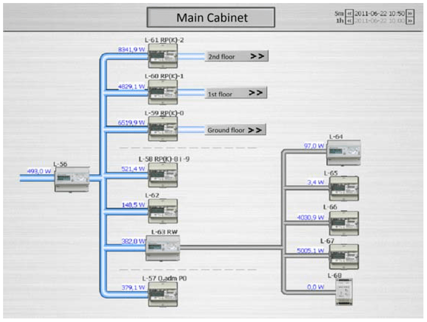
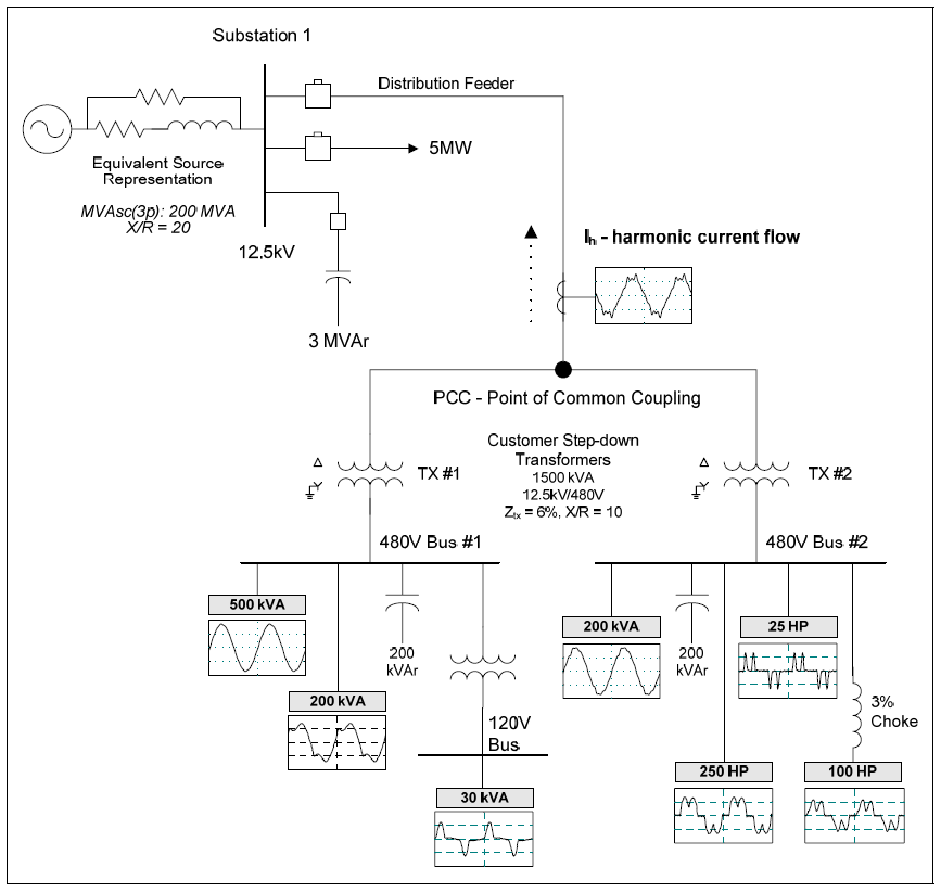
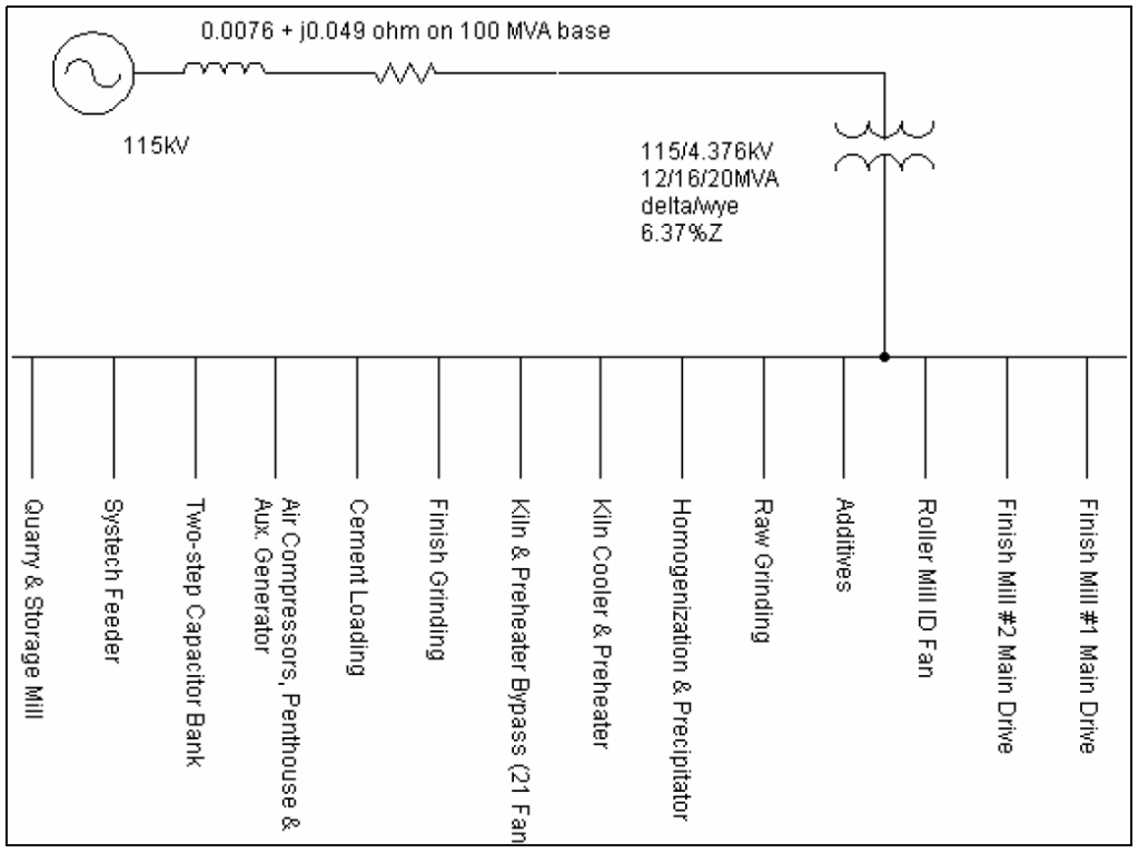
Measurements were performed at most of the 4160 volt feeders. Figure 1 shows a simplified one-line diagram for the plant electrical power system. The feeder current measurements were performed in the main switchgear room at the existing current transformers. The bus voltage for these measurements is the voltage measured at the potential transformer secondaries in the Incoming power cabinet.

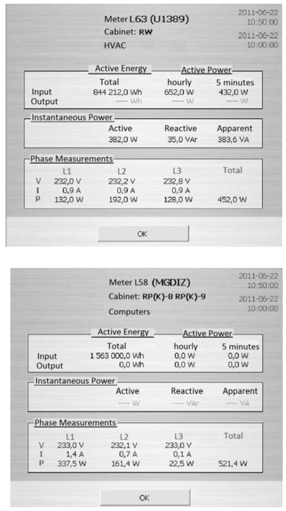
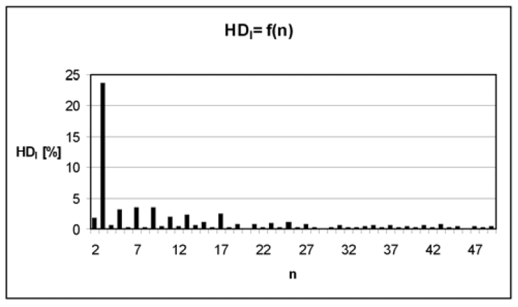
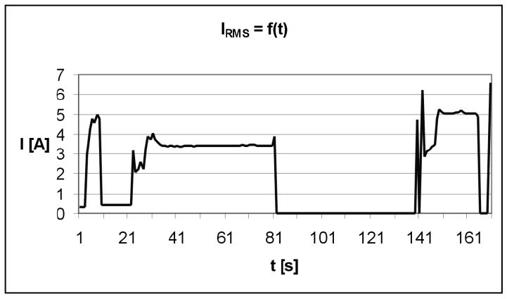
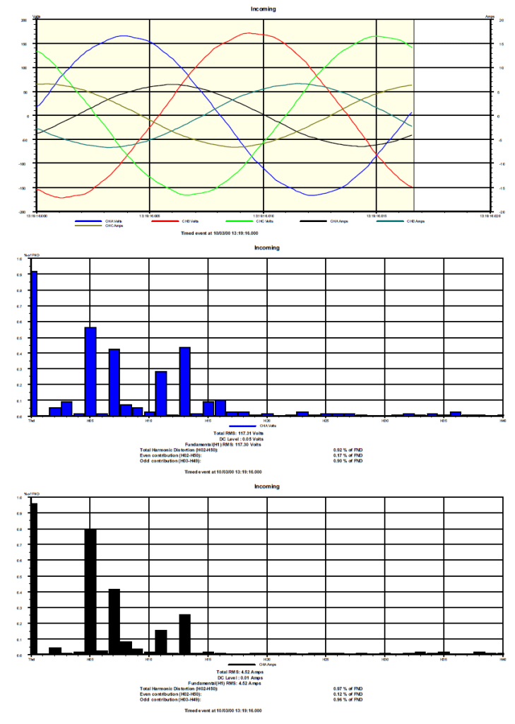
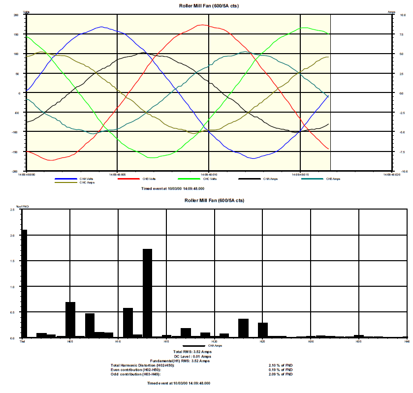
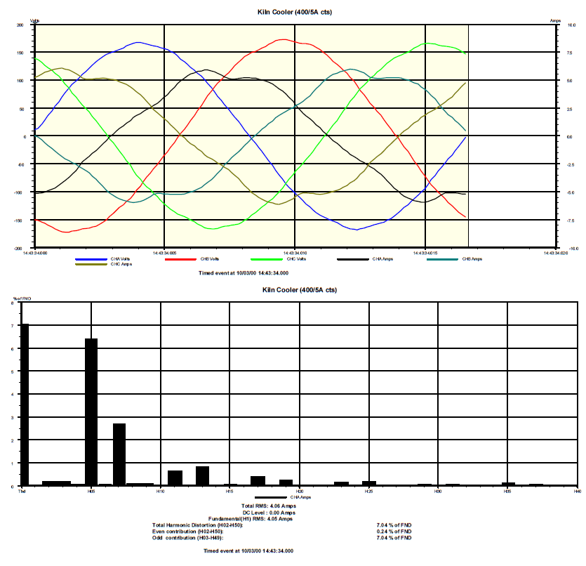
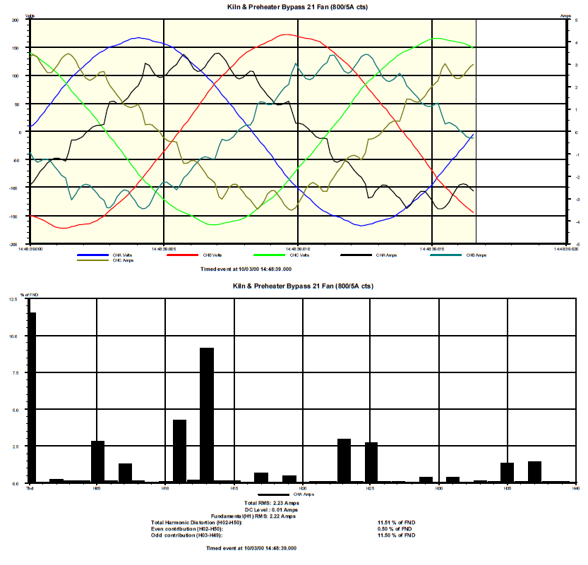
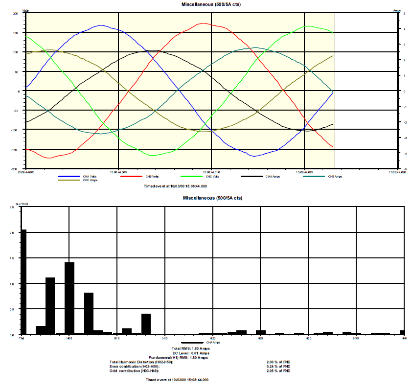
The measurement snapshots show the three-phase voltage and current waveforms and the harmonic spectrum for the Phase A current. The Phase A voltage spectrum is shown with the Incoming measurement snapshot.

Figure 1 – Electrical Power System One-line

Incoming

Finish Mill #1 Main Drive

Finish Mill #2 Main Drive

Roller Mill ID Fan

Raw Grinding

Homogenization & Precipitator

Kiln Cooler & Preheater

Kiln & Preheater Bypass (21 Fan)

Finish Grinding

Air Compressors, Penthouse & Auxiliary Generation

Figure 11 – Miscellaneous Measurement Snapshot

Two-step Capacitor Bank

Figure 12 – Capacitor Bank Measurement Snapshot

21 Fan

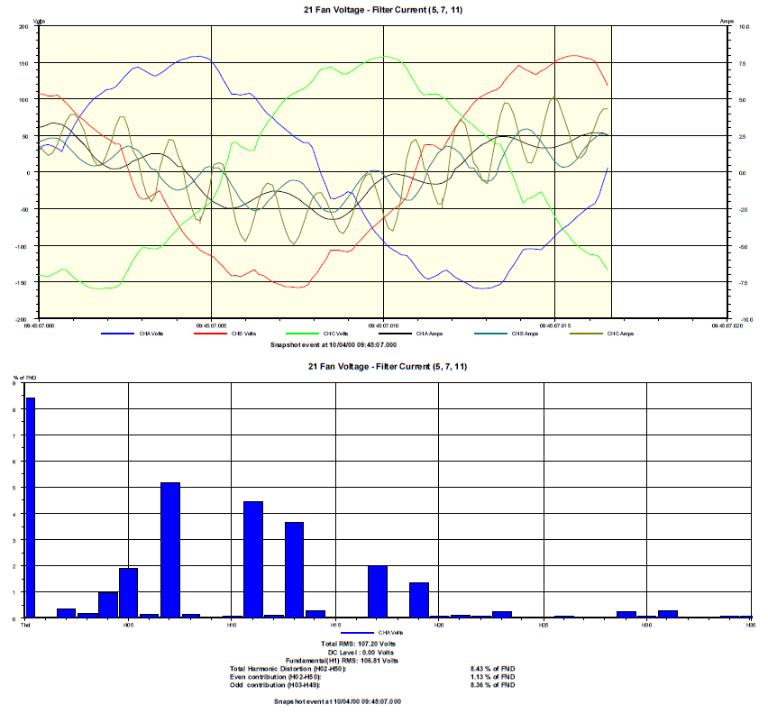
Measurements were performed at the supply to the 21 Fan and each of the harmonic filters. In Figure 13, Phase A current is one phase of the 5^th harmonic filter current, Phase B is one phase of the 7^th harmonic filter current, and Phase C current is one phase of the 11^th harmonic filter current.

Table 1 – Filter Current

	60 Hz	Harmonic	Irms
5^th	35	14	37
7^th	25	18	31
11^th	65	48	80

Table 1 shows a summary of the current measured at each filter. Filter current is characterized by the fundamental component and the harmonic component. The harmonic current in a filter is predominantly at the tuned frequency of the filter. The harmonic current in the 5th harmonic filter is 300 Hz current (5^th harmonic), the harmonic current in the 7^th harmonic filter is 420 Hz current, and the harmonic current in the 11^thharmonic filter is 660 Hz current. The fundamental current into the filters will increase as the bus voltage increases.

Measurements at the capacitor banks show that the capacitors are filters to higher order harmonic current, like the 13^th harmonic. Figure 12 shows the measurement snapshot of the capacitor bank current. 10 % of the capacitor bank current is 13^th harmonic current. This occurs because low impedance is created by the parallel combination of the capacitor banks and the system inductance. The system inductance is dominated by the substation transformer reactance.

The power factor correction installed at the 400 HP Roller Mill ID Fan creates a similar situation. The current measurements at the Roller Mill ID Fan feeder show 13^th harmonic current. Some 13^th harmonic motor current is not necessarily harmful to the motor. Bus voltage distortion and operating experience are the best indicators of potential motor problems caused by harmonics. Harmonic voltage distortion begins to seriously impact motor life when it reaches 8% to 12%, or higher. Another reason to not be too concerned about the harmonic current in the Roller Mill ID Fan feeder is that 13^th harmonic current is positive sequence current. Positive sequence current creates a field that rotates in the same direction as the field created by fundamental, 60 Hz, current. Negative sequence current (5, 9, 15 harmonic) is the greatest concern to motor operation

THD_V with Different Capacitor Bank Configurations

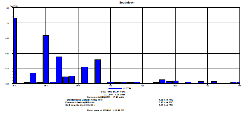
Figure 14 THD_Vwith Both Capacitor Banks On-line

Figure 15 – THD_Vwith One Capacitor Bank On-line

A comparison of Figure 14 and Figure 15 shows that the high impedance caused by the parallel combination of the capacitor banks and the system inductance moves from near the 7^th or 8^thharmonic to somewhere closer to the 13^th harmonic.

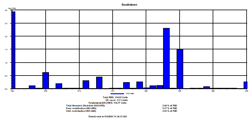
Figure 16 – THD_V with No Capacitor Banks On-line

Figure 16 shows that the system parallel resonance has moved to a higher frequency between the 20^thand 25^th harmonic.

The measurements show that the normal capacitor bank configuration, both steps on-line, is the best configuration as far as minimizing bus THD_V. It is not clear from the measurements how the capacitor bank configuration affects the 21 Fan harmonic filter current.

Figure 17 – Simulated System Impedance with different Capacitor Bank Configurations

Figure 18 – Kiln & Preheater Bypass Feeder Current

The chart of the Kiln & Preheater Bypass feeder current shows that the 13^th harmonic current is highest with one capacitor bank on-line, it is lowest with no capacitor banks on-line. These results coincide with the system impedance evaluations and with the voltage distortion recorded during the different capacitor bank configurations.

13^th harmonic current from the 21 Fan and from the Kiln Main Drive normally flows into the capacitor banks. The capacitor banks are filtering 13^th harmonic current.

HARMONIC SIMULATIONS

Electrotek developed a power system model for the facility and the associated utility power system. The model is used to simulate harmonic voltage distortion and to evaluate power system impedance with respect to power system configurations and equipment.

Simulations were performed to evaluate solutions that focused on improving the reliability of the process by eliminating the overload of the harmonic filters at the 21 Fan. Simulations are also used to evaluate the impact that specific solutions have on the entire plant power system and if solutions introduce any operational restrictions.

The simulations show that the harmonic filters at the 21 Fan are providing harmonic current control for the 21 Fan Drive and the Kiln Main Drive. Operational experience has proven that the harmonic filters are not designed to control the harmonic current from any loads other than the 21 Fan Drive. Calculations show that the filter design for application at the 21 Fan Drive alone is questionable.

Basecase

The harmonic simulations performed with SuperHarm were verified with the measurements that were taken at the facility. Measurements are used to create the base case for the harmonic simulations. The measurements that represent the worst-case harmonic current injected into the power system are used to develop the base case model. The base case represents “normal” conditions – both capacitor bank steps on-line and the plant operating with both finish mills running. The base case simulations are compared with the measurements to verify the accuracy of the model.

The simulated THD_V at the main 4160 volt bus is 1.22%.

Table 2 – Basecase Harmonic Filter Phase Current (amps)

Basecase – Present Configuration

Filter Current	Fundamental	Harmonic	RMS
5 h Filter	30.4	17.6	35.1
7 h Filter	22.3	16.1	27.5
11 h Filter	58.7	82.2	100.9

The table shows the phase current into each filter for the Basecase simulation. The results compare with the measured values.

5^th Harmonic Filter at 4160V Main Bus

A common approach to controlling harmonic current is to install a passive harmonic filter (or multiple filters). Passive harmonic filters are normally implemented at a main bus or where the voltage distortion problems are being experienced. The implementation of harmonic mitigation depends on many other considerations, like – initial cost of mitigation equipment, installation costs, operation costs, maintenance, control of equipment, space requirements, impact on the power system impedance, impact on other equipment, voltage rise, and resulting power factor. Distributing harmonic filters throughout a facility is usually more expensive to implement than consolidating the control of harmonic current at a main bus. It is more difficult to evaluate and control the operation of filters distributed throughout a facility.

This case evaluated the system with a 1500 kVAr harmonic filter tuned to the 5^th harmonic and a 2400 kVAR fixed capacitor bank. The idea is to utilize the fixed capacitor bank for power factor compensation and it also filters higher order harmonic current like the 13^th harmonic. The new 5^th harmonic filter would limit the amount of harmonic current into the 21 Fan harmonic filters from other nonlinear loads.

Table 3 – 21 Fan Filter Phase Current – 5^th Harmonic Filter at 4160V Main Bus

5h Filter at Main Bus

Filter Current	Fundamental	Harmonic	RMS
5th harmonic	30.3	17.7	35.1
7th harmonic	22.2	14.3	26.4
11th harmonic	58.4	78.6	97.9

Table 3 shows the simulated phase current into each 21 Fan harmonic filter. The simulations show that installing a 5^th harmonic filter at the main bus does not reduce the filter current during normal operation. The results suggest that the harmonic current into the filters from sources other than the 21 Fan and the Kiln Main Drive is normally very small.

New Feeder to Supply the Kiln Main Drive

Simulations were performed with a new dedicated feeder for the Kiln Main Drive.

The figure shows the present configuration for the supply of power to the Kiln Main Drive and a simple one-line diagram showing a new feeder for the supply of power to the Kiln Main Drive. The Precipitator ID Fan and the Quench Fan should also be supplied from the new feeder.

Table 4 – 21 Fan Filter Phase Current – New Feed to the Kiln Main Drive

New Feed to Kiln Main Drive

Filter Current	Fundamental	Harmonic	RMS
5 h Filter	30.9	6.1	31.5
7 h Filter	22.7	5.1	23.3
11 h Filter	59.7	80.6	100.3

The table shows that there is a significant decrease in the harmonic current into the 5^th and 7^th harmonic filters when the Kiln Main Drive is fed from a dedicated feeder and not tapped off of the 21 Fan feeder. The reduction in rms current correlates to the reduction in harmonic current.

New Feeder and 5^th Harmonic Filter at the Main Bus

Simulations were performed with a 1500 kVAr 5^th harmonic filter installed at the 4160 volt bus and with a new feeder to the Kiln Main Drive.

Table 5 – 21 Fan Filter Phase Current – New Feeder and 5^thHarmonic Filter

5h Filter at Main Bus & New Feed to Kiln Main Drive

Filter Current	Fundamental	Harmonic	RMS
5 h Filter	30.8	2.4	30.9
7 h Filter	22.6	3.0	22.8
11 h Filter	59.5	76.7	97.1

The simulations show that this solution results in the least amount of current in the 21 Fan harmonic filters.

The impedance between the Kiln Main Drive and the 21 Fan harmonic filters is increased when the Kiln Main Drive is supplied from a new dedicated feeder. The added impedance helps to decrease the harmonic current into the filters from the Kiln Main Drive. The 5^thharmonic filter at the main bus limits the amount of harmonic current to the 21 Fan filters from other plant drives.

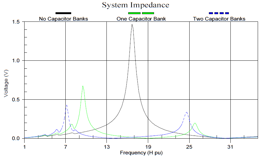
Frequency Scans

Frequency scans are performed to show system impedance as a function of frequency.

Figure 20 – System Impedance with 1800 kVAr & 2400 kVAr Steps

The figure shows that a parallel resonance exists between the 5^thand 7^th harmonic with both the 1800 kVAr and the 2400 kVAr steps on-line. Parallel resonances at characteristic harmonic frequencies (5, 7, 11, 13, etc.) should be avoided when applying power factor correction. The frequency scans also shows that a series resonance exists at the 13^thharmonic when both banks are on-line.

Capacitor banks will often detune themselves during operation when a parallel resonance at a characteristic harmonic causes voltage to rise high enough to cause individual capacitor cans to fail. Capacitors will fail until the parallel resonance moves away from the characteristic harmonic. As cans fail, the parallel resonance will shift to higher frequencies in the spectrum. High harmonic current in capacitors can also cause them to fail.

Figure 21 – System Impedance with Original kVAr and Present kVAr

Figure 21 shows how the system impedance has changed from the original compensation of 4200 kVAr to the present. The system impedance does not seem to have changed much, but plant operation and system configuration will affect the outcome of the interaction between plant loads and the system impedance.

An increase in system voltage can be the difference between a capacitor failing or not when a parallel resonance exists at a characteristic frequency. Bus voltage will increase at night, during the weekend, and when large loads are secured, like one of the mills at the plant. It is not certain what scenario caused capacitors to fail.

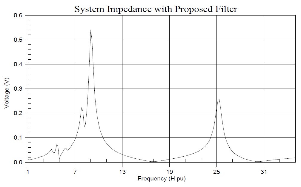
Figure 22 shows the results of the frequency scan with the 1500 kVAr 5^th harmonic filter at the main bus. The recommended filter creates a series resonance is at the 5^th harmonic. Compensation is added to the remaining capacitor bank to increase the total compensation of the bank to 2400 kVAr. 2400 kVAr of compensation places the parallel resonance near the 9^th harmonic.

Figure 22 – System Impedance with Recommended 5^th Harmonic Filter

Harmonic filters at various harmonic loads

The harmonic filters installed at the 21 Fan were not designed for application at the cement facility. The filters appear to be designed for the control of harmonic current injected by the 12-pulse A-B drive and nothing else. It is difficult to successfully apply harmonic filters at different harmonic loads. It is even more difficult to apply filters at one of several harmonic loads.

Applying harmonic filters at the drive is theoretically appealing because it limits harmonic current to the source. There is no easy, reliable, or relatively inexpensive way to implement this option. In order to avoid overloading, the filters often have to be installed with isolating reactors to prevent the flow of harmonic currents from other loads. This increases the cost of the individual filter installations. It is apparent that the filters are absorbing harmonic current from the 600 HP Kiln Main Drive. The filters are connected very close to where the Kiln Main Drive feeder taps off of the main Kiln & Preheater Bypass feeder.

The impedance of the long feeder from the main 4160 volt bus to the 21 Fan may limit the filter harmonic current from other ac and dc drives in the plant. How much current in the filters is from other drives depends on how many steps of the capacitor bank are on-line and what plant loads are operating.

Harmonic filters are usually applied at the main bus level when there are several harmonic loads. Even if the A-B drive were the only nonlinear load at the facility, the filters should be designed for reliable operation with 1.0% to 2.0% THD_V due to the utility supply.

RECOMMENDATIONS

1. Electrotek recommends that the Kiln Main Drive be supplied from a new feeder. The Precipitator ID Fan and the Quench Fan may be supplied from the new Kiln Main Drive feeder, also. Supplying the 21 Fan Drive and the Kiln Main Drive from different feeders will lower the current into the 21 Fan harmonic filters and will increase the reliability of the process. Performance of this recommendation may allow the client to forego the performance of Recommendation 5, the installation of a 2000 kVAr filter at the main bus. This is explained further with Recommendation 5.

2. The 5^th harmonic filter and the 7^th harmonic filter at the 21 Fan Drive have been detuned by utilizing the 105% tap of the respective filter reactors. The 11^th harmonic filter should be detuned also if it has not been. Calculations show that using the 105% taps on the 0.83mH filter reactors will decrease the current into the 11^th harmonic filter. This recommendation may be performed at any time.

3. The A-B 21 Fan Drive trips off-line when a harmonic filter overload trips because the harmonic filters do not have dedicated breakers to open and protect the filters. The same breaker serves as protection for the 21 Fan Drive isolation transformer and each filter. The company could improve the uptime of the 21 Fan Drive and the plant process by serving each filter through a dedicated breaker and removing the interlocks between the filter overloads and the main breaker. It makes sense to control what filters are on-line at the same time and there are filter combinations that should not cause the 21 Fan Drive to trip.

These filter configurations could be permitted during drive operation:

1. All three filters off-line.
2. 5^th harmonic filter on-line.
3. 5^th and 7^th on-line.
4. 5^th and 11^th harmonic filters on-line.
5. 11^th harmonic filter on-line.
6. All three filters on-line.

This recommendation may be performed at any time.

4. The amount of compensation that should be installed as a fixed capacitor bank is 2400 kVAr. The one-line drawing shows that one step of the capacitor bank used to be 2400 kVAr. This recommendation is to operate with one 2400 kVAr step on-line. 2400 kVAr is a good amount of compensation because the system parallel resonance is near the 9^th harmonic. The 9^th harmonic is acceptable because it is in between the characteristic 7^th and 11^th harmonics.

This recommendation can be performed at any time. It appears that this could be performed by company personnel and requires no material expense. Capacitors could be removed from the other capacitor bank (the 1800 kVAr bank) to increase the compensation of the 2400 kVAr bank back to its original value.

5. The old 1800 kVAr capacitor bank should be converted to a 2000 kVAr 5^th harmonic filter. Electrotek recommends that the filter be tuned to 297 Hz. The recommended filter is designed with 4800 volt capacitors so the effective compensation of the filter will be about 1560 kVAr. The harmonic filter at the main bus will greatly reduce the amount of 5^th or 7^th harmonic current into the 21 Fan filters from other adjustable speed drives. The filter design specifications are included in the appendix at the end of the report.

This recommendation does improve on all of the other recommendations, but it may not be necessary after the Kiln Main Drive is supplied from a new feeder. Electrotek suggests that the company implement Recommendation 1 and evaluate the operation of the 21 Fan Drive and the harmonic filters. The evaluation should include measurements at the 21 Fan harmonic filters for at least one week. The evaluation may show that the investment in a 5^thharmonic filter may not be cost effective.

6. A harmonic evaluation should be performed before the plant substation is upgraded or before major equipment or system changes are made. Examples of things that will need to be evaluated are:

– 1. System Impedance. Determine where the parallel resonance is that is created by the parallel combination of the 2400 kVAr fixed capacitor bank and the system inductance. The substation transformer greatly influences the system inductance and the resulting system impedance.

– 2. Determine the affect that new loads or a new substation transformer will have on the loading of the 5^th harmonic filter, the 21 Fan filters, or the harmonic voltage distortion.

It is very important that this recommendation is applied. Electrotek will be happy to provide the company with advice on whether or not a harmonic evaluation or an engineering study needs to be performed. This advice is free of charge.

Appendix A: Filter Design Spreadsheets

RELATED STANDARDS
ANSI/IEEE Std. 18-1980: IEEE Standard for Shunt Power Capacitors
IEEE Std. 1159 – 1995 Recommended Practice for Monitoring Electric Power Quality
IEEE Std. 519-1992: IEEE Recommended Practices and Requirements for Harmonic Control in Electrical Power Systems

GLOSSARY AND ACRONYMS
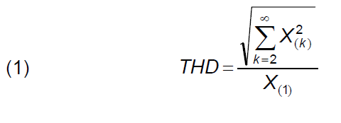
THD: Total Harmonic Distortion

Active Consumers in Smart Grid Systems – Applications of the Building Automation Technologies

Published by Marian NOGA¹, Andrzej OŻADOWICZ¹, Jakub GRELA¹, Grzegorz HAYDUK¹,
AGH Akademia Górniczo-Hutnicza, Wydział Elektrotechniki, Automatyki, Informatyki i Inżynierii Biomedycznej (1)

Abstract. The Building Automation Systems (BAS) fulfil an increasingly important role in buildings, especially commercial and public buildings. They are an essential element of the building management systems (BMS) organization, integrating all building infrastructure subsystems on the field level. This paper presents the concept of using BAS systems in organization of local energy and the media consumption measurement network, in view of the remote metering Smart Metering and Smart Grid implementation as well as emergence of so-called prosumers.

Streszczenie. Systemy automatyki budynkowej (BAS) spełniają coraz bardziej znaczącą rolę w budynkach, zwłaszcza komercyjnych i użyteczności publicznej. Są podstawowym elementem organizacji systemów zarządzania budynkami – BMS, integrując na poziomie obiektowym wszystkie podsystemy infrastruktury budynkowej. W artykule przedstawiono koncepcję wykorzystania systemów BAS w organizacji lokalnych sieci pomiarów zużycia energii elektrycznej i mediów, w perspektywie wdrożenia systemów zdalnego opomiarowania Smart Metering, inteligentnych sieci elektroenergetycznych Smart Grid oraz pojawienia się tzw. prosumentów. (Aktywni odbiorcy w systemach Smart Grid – aplikacje technologii automatyki budynkowej).

Słowa kluczowe: automatyka budynkowa, LonWorks, integracja, SmartGrid.
Keywords: building automation, LonWorks, interoperability, SmartGrid.

Introduction

The electrical power systems need modernization and adaptation to new conditions of their functioning. First of all it is connected with growing energy demand, reducing system reserves and more and more popular using of renewable sources of energy. They are going to be connected to the power systems in different, random points, additionally with different power level. It brings changes into power distribution system and its load. Since it is important to implement more dynamic energy management in the power system as well as monitoring and improvement of power quality parameters. Information about the power level in the electric power system regions and changing energy demands is needed. These questions are base for the Smart Grid idea – the traditional power grid with some main power plants will be transformed into interactive, distributed power network. Power distribution in this kind of network will be depend on active consumers demand (demand data, energy consumption monitoring, different tariffs) as well as energy distributors and local generating points (wind turbines and PV panels farms etc.) The Smart Grid it is not only buzzword, but the first of all huge chance to improve energy efficiency, energy consumption minimization, appropriate energy management and power grid improvement. To put it simply, Smart Grid it would be hybrid of the energy distribution system and IT networks to provide bidirectional communication between all modern electrical power system subjects. The first element of this conception should be intelligent, remote measurement system of energy and other media consumption – Smart Metering. This kind of system contains: electronic, intelligent meters, data transmission infrastructure, database and management system with bidirectional, real-time communication [26]. Information from main and local power plants are transmitted to the individual and commercial consumers (supply parameters, energy quality parameters) and from consumers to the providers (power demand, failures, problems) [10,26,27]. This way classic consumer could be prosumer with possibility to active manage energy consumption (switch loads out of peak load/maximum demand; different tariffs) and produce and sale energy to the grid. Consumers are usually connected with different kinds of the buildings (houses, offices, industrial buildings, supermarkets, entertainment centers etc.). Very often they are equipped with IT infrastructure and more often building automation and BMS systems as well. It concerns especially public, office and commercial buildings [2,14].

Since it is very important and current question: to select tools and standards for Energy Service Interface (ESI) – software and hardware platform of communication and activity between prosumers, providers and producers in the buildings ESI could work as a part of the BMS or BAS (Building Automation System) system and in the houses as a part of the EMS (Energy Management System) or HAN (Home Area Network) networks [11,29].

Development of the Smart Grid is directly connected with implementation of new electric, electronic, automation and IT technologies as well as working out suitable directives, laws and standards. Progress in both fields should be systematic and simultaneous, especially taking into consideration current and binding directives and strategic programs accepted by the European Union.

Legal regulations

The question of the Smart Metering systems implementation was first time brought up in the European Parliament and of the Council Directives. First of them No. 2006/32/WE concern on energy end-use efficiency and energy services. it is state there that Smart Metering systems, with individual meters for each consumer, are one of the means to achieve energy efficiency in European countries. There are general regulations for measurements and energy savings verification there as well. The second one is Directive No. 2009/72/WE concerning common rules for the internal market in electricity. In this document the Smart Metering systems are mentioned as a tool to achieve main directive goals: creating competitive and safe electrical energy market with consumer protection [6]. The directive states that consumers should have access to their energy consumption data (consumer is owner of the data) and data should be available for energy providers (other regulations). This statement resulted in necessity to work out new regulations in the personal data protection field and data security in the IT and transmission systems as well as on the filed level (direct connection between devices and meters in the automation systems) [29]. In the Directive there is on very important thread – in Annex I it is stated that each country implementation of the Smart Metering systems for the electrical power supply may be subject to an economic assessment of all the long-term costs and benefits to the market and the individual consumer or which form of intelligent metering is economically reasonable and cost-effective and which timeframe is feasible for their distribution. Such assessment shall take place by 3 September 2012. Where roll-out of smart meters is assessed positively, at least 80 % of consumers shall be equipped with intelligent metering systems by 2020 [2,7]. To carry out mentioned assessment in Poland special team for the Smart Grid implementation questions have been appointed by the Minister of Economy at 6^th of December 2010.

At the December 2011 this team have announced positive recommendation to implement intelligent measurement systems – Smart Metering in Poland. It resulted in preparing special new regulations to amended energy law (pol. Prawo Energetyczne) and obligate distribution network operator (pol. OSD – Operator Sieci Dystrybucyjnej) to install intelligent meters for all consumer to 31^st December 2020 [25,28,33]. It is worth to emphasize that the team have proposed the Minister of Economy to withdraw from detailed analysis of cost-effectiveness of the Smart Metering implementation. The Member of Parliament and the chairman of a parliamentary committee for power and energy industry – Mr. Andrzej Czerwinski explains that preliminary assumptions to the Smart Grid law and implementing regulations had been prepared earlier and some pilotage installations had been implemented in Poland by different energy providers, so positive recommendation have been natural step in that situation [5,7,34]. The faster way to implement the Smart Metering idea have been opened. In April 2011 a law on energy efficiency was passed – it obligate entities operating in the energy industry to take action to improve the energy efficiency factor and obtain the so-called “white certificates”. However, from the point of view of the Smart Grids and Smart Metering concept development more important are legislative work of the Ministry of Economy, associated with the development of so-called Smart Grid Law within the amendment of the Energy Law. Main objectives of the mentioned amendment are [5]:

• Reducing peak demand for the power and ensure balance in the National Power System
• Development of a competitive electricity market through introduction of billing based on the actual consumption profile with facilitation of change the provider
• Provide information about the current energy and other media consumption
• Limiting in electricity prices increases for end-user through the implementation of new competitive forces in the electricity market.

These objectives have been the subject of extensive sectorial and social discussion, undertaken in the relevant documents, among others by the President of the ERO (Energy Regulatory Office). In one of them the concept of the Smart Metering market in Poland is outlined, with indication of the different actors role and requirements for the Independent Measurement Operator. This name in the latest documents proposed by the Energy Regulatory Office has evolved to the following: Measurement Information Operator [35]. As already mentioned, particular concern is dedicated the customers who in the new concept of operation of the power system, will become the active players, with an appropriate level of independence and the right to dispose of the data on energy consumption and demand. The aware consumer should be able to choose their electricity supplier/provider and to sale energy produced from renewable sources – acting as a prosumer. Additionally, attention is drawn to the fact that modern Smart Grid systems should increase the safety and reliability of the whole power system and energy supply to the customers. It is assumed to introduce monthly billing for electricity, based on actual measurements of the short-term consumption [25,36]. Many of these aspects were also discussed in a study on the implementation of the Smart Metering in Poland [13], with detailed analysis of the objectives, costs and benefits of this process. According to the authors, the main objective of implementation is to meet the requirements of the European Parliament and of the Council directives and to ensure energy security, with the least social cost. Reference is made to the fact that intelligent energy system should be stable and better balanced, ensuring the full support of renewable energy sources (RES) connected to the power grid and improving power quality. It was also established several key functional requirements that should provide the smart grid system. Each is now considered as a separate issue: the availability of data in relation to privacy and protection of personal data; the choice of tariffs and energy suppliers in the light of competition in the energy market and the already mentioned issue of the energy sale to the system, in the perspective of a bi-directional meters implementation. There is emerging conflict of interests of different social groups, industry and market. It turns out that energy consumers are primarily interested in reducing bills and simultaneously suppliers and manufacturers – profit and market share maximization. From the industry point of view even more considerable conflict is the pursuit to stabilize and better balancing the power system form the producers side and the possibility to easy connect the renewable sources to the system from independent producers – prosumers side. These issues should be explicitly addressed in the new law and related regulations [13,28]. In current sectorial debate associated with the inevitable necessity of Smart Metering systems implementation, the two main trends are outlining. One, created around the position of the President of the ERO and the Distribution Network Operators (DNO). Second, generated on the basis of the advisory team of the Ministry of Economy findings and propositions for the New Energy Law. Experts point out the need to synchronize the activities and positions of these two trends. It would be prerequisite for the future development of a uniform system of the intelligent power grid, both in the field of instrumentation, control and information sharing [32].

Active consumers – prosumers

In all discussions about a legal for the development of Smart Metering, the questions of the need to activate consumers and carry out extensive public information campaigns are raised. Active consumers are key to the Smart Metering and the Smart Grid idea success. To activate them good information campaign is needed about benefits, possibilities, functionalities and requirements connected with smart meters installing. But even the best organized information actions will not bring desired results if they will not follow a specific (not necessarily large) the benefit for the consumers, which motivate them to engage in the idea of energy saving and improve efficiency. The Smart Grid and intelligent power grid will retain and use its enormous potential, only with the approval of the customers. While significant progress has been made in the efficiency and reliability of the energy system, largely due to the modernization of transport infrastructure network, changing customer behaviours and their demands, remains a very difficult, particularly if they are not convinced of the benefits awaiting them. There are different kinds of benefits [17,25]:

• Simplification of settlements with customers
• Energy bills based on actual energy consumption
• Ability to change and adjust power tariffs to the “profile” of the energy consumer
• Increasing the efficiency of the power supply and distribution systems
• Simplify the process of energy supplier changing
• Increased protection of the so-called vulnerable customers (network performance monitoring)
• Increase public awareness on energy consumption, effectiveness and savings.

But installation of smart meters it is not everything – it is the only necessary tool. It should be implemented market mechanisms in the energy sector as well – not only in sale for large industrial consumers and institutions, but also for the smaller, individual consumers. Only such action, including mentioned previously awareness-raising actions, should result in the involvement of them, encourage to rationalization of the energy consumption and invest in renewable sources. Otherwise, it may be that Poland will be in the same situation as some of European countries, such as Italy, where in recent years a large-scale smart meters installations have been introduced (about 40 million customers) and the social awareness of their possibilities and functionalities increased only about 5% to 10%. In this situation the smart meters capabilities are used mainly by energy suppliers to detect and eliminate energy theft and power system balancing [27].

Another question connected with consumer involvement is personal data protection. It is often emphasized by energy sector experts and the Inspector General for Personal Data Protection [5,13,38]. As it was mentioned before the energy consumption data of the consumer are his own. This issue does not seem to be discussed, but energy consumption data should be collected remotely by the provider or Measurement Information Operator. Therefore, it should be properly take into account in the energy supply contracts [11,36]. From the other side data from meters should be available for the consumers to browse them both directly and processed – reports, analysis, profiles of the energy consumption etc. The different concepts of that supplier-operator-consumer interaction are verified in the pilot projects and the existing smart metering systems in Europe. One idea is to provide customer specific portable modules with wireless communication to track current consumption and effects of different types of devices activation at different hours of the day (peaks, tariffs). Another idea is based on the use of modern mobile phones, tablets and television sets with corresponding applications, dedicated to communication in a local network HAN (Home Area Network called) by different standards such as Bluetooth, Wi-Fi or TCP-IP –Internet [12,16]. However, it seems that one of the best solutions, to simplify service and allow remote access to measured data is setting up of virtual consumer accounts on websites provided by the Measurement Information Operator. Many attempts are made in this field in Western Europe and the USA. This kind of websites offer wide range of possibilities to browse reports, analyses, current meter readings, tariff selection and energy charges in on-line mode. From the average consumer point of view these features allow self-control and verification of actions taken to improve energy efficiency. Good example in this field is website Google Power Meter provided by Google for one of the pilotage projects [1,9]. But the convenience of the use of such services is governed need to ensure a high standard of data security, control access and protect against unauthorized access attempts.

The active support of energy systems – key elements

Previously mentioned the active energy consumers are only one part of the planned active, dynamic power system – Smart Grid. The implementation of this idea requires a number of elements: support and data transmission organization between all elements of the system as well as modernization and installation of modern system that will be control power in the supply system, according to changing demands. This also applies to technologies, systems and infrastructure in buildings, which are among the most intensive consumers of electricity and heat. Around the world, the steps are taken to enable commercial and other buildings interact with smart electricity grids. These actions will allow the users to directly participate in the energy market, with increased emphasis on energy savings and improve power management. This concept is called the Building-to-Grid or B2G [11].

One of the emerging Smart Grid standards allowing buildings connection to the network is OpenADR (Open Automated Demand Response). OpenADR is an open and standardized method of communication signals about energy demand (called DR – Demand Response) [2,22]. This data is for the electricity providers, system operators and their customers and should be communicated by means of a common language with the use of existing network based on IP protocol, such as the Internet. It is worth noting that the number of buildings equipped with an Energy Management System (EMS) is increasing, so they are ideal platforms for the implementation of demand response energy consumption (OpenADR). Such objects can use or modify existing intelligent network control to accept signals from the OpenADR systems. With preprogrammed set of events, building automation system can reduce the load according to the messages received in real time and provide information about its use of energy back to the energy supplier and operator. To allow the EMS systems receive signals from the OpenADR will likely require software update or installation of additional equipment, the purpose of which will provide relevant information to the building management system [11]. One of the most critical issues is appropriate programing of energy control strategy in the EMS. This system must react accordingly depending on the message coming from the OpenADR, which can include information about the incident or the current and projected energy prices. For example, if the message contains information about the growth rate for electricity, building automation system can dim the lights or change the temperature settings to reduce the energy consumption – heating or HVAC system [10]. Leading organizations caring for distributed smart grid standards are actively involved in the development of Smart Grid system through several industry initiatives, including:

• The standards of building automation should be considered as a tool for the Smart Grid system realisation. The main objective of this process is to ensure that products comply with the standard can be used in many cases recommended for use in the smart power grid projects

• Adaptation of the standard to the B2G idea and the appropriate type of communication with the OpenADR. This process is designed to make the most effective use of the systems properties and ensure their mutual cooperation

• Mobilization of the operators, distributors, integrators and consumers, primarily to increase their awareness about the capabilities of the Smart Grid.

Building automation systems as part of the active customers infrastructure

So far, the building automation system integrators have been concentrated primarily on providing users with the appropriate comfort and safety in buildings. Thus, common functionalities and features in automated buildings include: lighting and lighting scenes and scenarios control, service of blinds and shutters in windows, HVAC control – thermal comfort, access control, monitoring of devices and subsystems operating parameters, monitoring and acquisition of events, cooperation with anti-theft and fire systems, etc. In larger buildings these functionalities are more and more integrated and implemented into a single building management systems – BMS. In this kind of the applications, building automation systems have been used for many years, and their functionality in this field is still improving. They are becoming more reliable, and users derive benefit from them more and more confidence. The purpose of installers and integrators of the automation and monitoring systems is to achieve such a state that users use them involuntarily and the building infrastructure devices perform their functions reliably and quickly. According to the AGH researchers building automation systems can be used at field level as a tool for monitoring and optimizing the electrical energy and other media (heat, gas, water) consumption. It could be achieved by introduction of integrated remote metering modules and control procedures as well as mutual interaction between the different subsystems installed in the modern buildings [20].

Pilotage and research installations – examples and case studies

Taking into considerations presented information and directions of building automation systems development, to implement them in the Smart Metering and Smart Grid applications, AGH scientists and research workers undertaken research in the field of the building automation systems used to perform tasks connected with implementation of the Smart Grids. At AGH in Krakow is conducted project: “Optimising energy consumption in buildings”, funded by the National Research and Development Centre (NCBiR). In this project have been implemented comprehensive systems of the electricity consumption metering in three buildings – one in the AGH Krakow campus and two in the office and commercial complex. One of the buildings is built as so-called energy-efficient, using the latest building and telecommunications technologies [10].

Define the parameters of the energy consumption of buildings analysed in the project, with different groups of receiving energy, have required proper metering. To achieve this, three systems of energy consumption monitoring have been developed, for all three mentioned types of buildings. The first one is educational and office pavilion B1 AGH from the 50’s of last century. Another one is a No. 6 building with traditional technologies located in Science and Technology Park Euro-Centrum (PNT) and the last one is energy-efficient building No. 7, also located within the PNT [20]. The most detailed metering installation is in the building No. 7 PNT. The monitoring energy consumption system has been developed and implemented using the existing supply network topology, including among others meters for: individual lighting circuits, computer and power sockets both for groups of rooms (some rooms for one tenant) as well as power circuits of technical infrastructure in the building, such as a heat pump, heat exchanger, chiller, central HVAC, elevators. Monitoring system has a tree structure, including the main meter, the meters in the floor cabinets and ultimately individual meters for groups of rooms. An important element of the monitoring was to develop a system of data acquisition, reading all the meters in a 5-minute periods, and designating the difference in readings (5-minute power/load). Additionally, if the meter allows the measurement of other parameters such as voltage, current, reactive power, they are also recorded in the system. The data acquisition system is carried out on computers and servers at AGH Krakow with the building No. 7 PNT remote data communication via the Internet network. To present the collected data, visualization has been developed, allows to display 5-minute and hourly measurements from each meter of any moment of time. The visualization includes meters installed in both the main switchboard as well as floor cabinets on the ground, first and second floors. The window of visualisation display meters for the main switchboard is shown in Figure No. 1. ¹⁾ It shows the structure of the monitoring system with 5-minute power indicators for each meter for preset time/moment. The visualization allows to observe and analyse the data form any time, with the possibility of moving about five minutes or one hour [3,23].

Fig. 1 – View of the monitoring visualization with energy meters in main switchboard

The metering system have been built using energy meters of different companies. Some types of the meters, such as U1389, allow direct data collection through a bus with international standard of building automation system – ISO/IEC 14908 (LonWorks®) [4]. Others, having only a pulse outputs, are connected to the LonWorks building automation system by appropriate modules, used to convert pulses to LON standard network variables (SNVTs). With the developed visualization system is also possible preview of all recorded parameters for each meters [3] ¹⁾. In Figures No 2a and No 2b two views of parameters form different kind of meters are presented.

Fig. 2a i 2b – An example views of the details form energy meters

Experience with implementation of the remote metering system in these buildings point to that the network building automation systems could be successfully used as a tool for organization and implementation of the Smart Metering systems, particularly in perspective of integration them with the BAS or EMS systems on the field-level. Therefore, if in buildings is infrastructure of the building automation systems, always should be considered use it to carry out mentioned tasks and functions. A very important features of the bus, international building automation systems (LonWorks, KNX, BACnet) are openness and distribution, simplify integration of the measurement and control monitoring infrastructures in one building management system BMS [24,37]. By this system it is possible to check on information from different meters and correlate it with optimal control scenarios and algorithms. It could be use also to identify areas with the greatest potential of energy save and improve energy efficiency of whole building.

It is worth noting that the mentioned Smart Metering systems have not been implemented with data collection protocol in accordance with IEC 62056 (successor to IEC 61107), dedicated to smart metering applications [30]. The measuring system have been performed using a network compliant ISO/IEC 14908, mainly used for building automation systems and in industrial automation, with option of standardized data transfer over the Internet. Use of the ISO/IEC 14908 standard infrastructure instead the IEC 62056, contributed to an easier and faster implementation and avoid the additional costs of metering and control systems installation. Recording and reporting of data was carried out using the public, free software tools, with development of own methods for processing the data. As a result, the installation allows for implementation of the Smart Metering functions:

• Identification of the distribution of energy consumption per day for all the buildings and the selected areas (floors, rooms)
• Presentation of the energy consumption in different forms: graphs, trends and reports
• Identify the areas with the greatest energy consumption of electricity, etc.

The system allows use of its architecture and structure to almost directly implement for monitoring and reporting of other, new buildings.

Another example of use the building automation systems as a tool to support the active energy consumers – mainly buildings’ users, is organizing of an energy management system in the buildings – EMS. This kind pilot system is implemented and researched in Certified Laboratories Network for Energy Efficiency and Building Automation – AutBudNet in AGH Krakow, equipped with infrastructure of the building automation system and BMS, based on the European and international standard ISO/IEC 14908 (LonWorks) for distributed control system [4,18,21,29,31]. With this infrastructure, it is possible to implement classical building automation functions such as lighting and heating control, access control, and more. Additionally, the automation system can operate on the field level and the remote monitoring and management of different sub-systems: fire extinguishing system, CCTV, remote meter reading of electricity consumption and heat, monitor the operating parameters of the solar collectors and PV panels. It allows use laboratory rooms as real object for research of functionalities and features of building automation systems and their influence on operation of the buildings [21,37].

In the current design practice for the building automation systems commonly used solution is implementation of different building infrastructure subsystems as autonomic installations and their integration is not possible at field level, but only at higher levels of the building management systems organization. In addition, most energy and media monitoring systems are carried out completely independent of the building automation (the intelligent control of building resources), commonly only for accounting purposes, for the suppliers of energy and media as well as costumers. It generates limitations in functionality and possibilities to devices, sub-systems cooperation. The open building automation system implemented in the AutBudNet laboratories allows integrating devices on the lowest, field level and data exchange is faster, more effective, without higher levels of monitoring and management systems. Research conducted in the AutBudNet laboratories confirm the thesis that implementation of new, distributed control systems, based on international standards, provide reduction of energy consumption in buildings by integration all automation features and functionalities and cooperation different devices and sub-systems [10]¹⁾. In the latest research several scenarios have been prepared for optimization of energy costs, depend different energy prices at different periods of days [8]. Monitoring of the control system in these scenarios as well as observation and analysis of the effects of optimization, required to organize the installation and integration of the existing energy consumption monitoring system (Smart Metering) and the energy management system (EMS). The last one cooperate with touch panels LVis by Loytec with graphical interface for user and TCP/IP and LonWorks standard interfaces for communication. Thanks this LVis panels could be connect to the BAS network directly on the field level (for example direct data exchange with meters) and remote controlled – TCP/IP communication with PCs, tablets or smartphones. For LVis panels suitable control screens have been prepared to present data from different devices and subsystems. They are presented on the 3 and 4 figures.

Fig. 3 – The LVis panel screens with selected functions and parameters from EMS.

Based on the presented system for monitoring electricity consumption with integrated subsystems of the building infrastructure, currently are conducted research aimed at long-term measuring the level of consumption in particular electrical equipment groups in the building laboratory infrastructure and their analysis¹⁾. Research workers try different new settings and correct earlier applied settings to obtain optimal work conditions – maintain comfort in rooms with a maximum reduction of energy consumption. In addition, there are verified opportunities for EMS system cooperation with different elements of HAN network – remote PCs and mobile devices, designed to support user (presentation of data, access to interim analyses, reports, energy consumption, etc.) [3,12,15,16,18]. An integral part of these networks is object-oriented communication standard LonWorks – dedicated to the building automation and increasingly used in public and commercial buildings (offices, sports and entertainment centres, etc.).

Conclusions

From the first experience, building automation systems could become an integral part of communication infrastructure organization for the Smart Metering systems in buildings. Particularly noteworthy is the ability to integrate measurement systems with building automation components in the field level. This is very important especially in larger buildings, commercial and public, where usually network infrastructure for automation and monitoring have been installed. With the mentioned integration, this infrastructure could be used for organization of the local Smart Metering systems. The user has ability to monitor energy and media consumption in building, with possibility to dynamic impact on the building infrastructure facilities integrated in the single system EMS, allowing to optimize the energy and media consumption. In addition, advanced routers and servers, dedicated to building automation, also allow remote operation with monitoring and control systems, providing user with free access to measurement data and to make the necessary changes, settings, etc.

Therefore, it is worth remembering the building automation standards in determining guidelines and standards for communication protocols, dedicated to the Smart Metering systems, especially for commercial and public buildings as well as dwellings. They allow for much easier integration of measurement systems with the overall power management system (EMS) and the whole building management systems (BMS). In perspective introduction of dynamic and interactive energy management systems (Demand Response), integration with the building automation infrastructure will enable to realize automated response procedures for all subsystems and equipment in buildings. Impulses that trigger these reactions would be outside signals – from the Measurement Information Operator, supplier of energy/media or the settings made by the user directly in the system by HAN or BMS. Importantly, part of these activities will be done automatically, without user involvement, but only with signalling events and changes in the visualization panels or dedicated websites [12,16].

In the coming years in the AutBudNet laboratories and other AGH-UST buildings, will be conducted further research on implementation of the building automation systems in the area of optimizing energy and other media consumption in the buildings and testing of various components of the Smart Metering for different types of the buildings. The results of these research and case studies, carried out on real objects with the modern infrastructure and devices integrated on the field level with international building automation standards, are quite significant. This is confirmed by strenuous activities of the U.S. and European organizations responsible for development and protection of these standards. They are engaging in any initiative on development of the Smart Metering and Smart Grid systems. Firms associated with these organizations the dominant product group are solutions and technologies to support implementation of the Smart Metering and Smart Grid, and allowing them to integrate with building automation systems. It seems, that in the coming years, this kind of application of the international standards for distributed and building automation will dominate in the field of the building automation and functionality of the EMS, BMS systems development.

¹⁾ Prace prowadzone w ramach zadania badawczego nr 5 Narodowego Centrum Badań i Rozwoju: „Zoptymalizowanie zużycia energii elektrycznej w budynkach”, w strategicznym projekcie badawczym: pt. „Zintegrowany system zmniejszenia eksploatacyjnej energochłonności budynków”.

REFERENCES

[1] Arizona Power Service; Strona WWW. Arizona Power Service. http://www.aps.com/main/services/myacctinfo/default.html#
[2] Billewicz K.: Smart Metering. Inteligentny system pomiarowy; ISBN 978-83-01-16809-4 Wydawnictwo PWN, 2012
[3] Chiang T., Natarajan S., Walker I.: A laboratory test of the efficacy of energy display inteface design; Energy and Buildings 55 (2012) 471-480
[4] Colmenar-Santos A., Teran de Lober L., Borge-Diez D., Castro-Gil M.: Solutions to reduce energy consumption in the management of large buildings; Energy and Buildings 56 (2013) 66–77
[5] Czerwiński A.: Przygotowywane prawo energetyczne – projekt ustawy o inteligentnych sieciach; Seminarium “Uwarunkowania wdrażania Smart Meteringu – problemy prawne, technologiczne, społeczne”. 12.04.2012 Warszawa
[6] Darby S.: Smart metering: what potential for householder engagement? Building Research & Information, 38: 5, 442 — 457
[7] Dyrektywa 2006/32/WE Parlamentu Europejskiego i Rady z dnia 5 kwietnia 2006; Strona WWW: http://eur-lex.europa.eu/pl/rok 2012
[8] Escrivá-Escrivá G., Segura-Heras I., Alcázar-Ortega M.: Application of an energy management and control system to assess the potential of different control strategies in HVAC systems; Energy and Buildings 42 (2010) 2258–2267
[9] Google Power Meter; Strona WWW. Google Power Meter. http://www.google.com/powermeter
[10] Grela J.: Inteligentne Sieci Rozproszone – technologie dla Smart Grid; Materiały Konferencyjne – artykuł; VII Konferencja Naukowo-Techniczna SIECI 2012 – Sieci elektorenergetyczne w przemyśle i energetyce. ISBN: 978-83-935801-0-1
[11] Haaser B.: Are you ready for Smart Grid? LonMark Magazine, April 2012, vol. 5, Issue 3
[12] Han Y., Xu L.: A survey of the Smart Grid Technologies: background, motivation and practical applications; Przegląd Elektrotechniczny, ISSN 0033-2097, r. 87 nr 6/2011
[13] Instytut Energetyki Oddział Gdańsk, Ernst&Young Business Advisory: Studium wdrożenia Smart Meteringu w Polsce; Platforma Informacyjna Inteligentnego Opomiarowania – Strona WWW: http://www.piio.pl – Gdańsk, 6 maja 2010
[14] Jaworska E.: Euro 2012 – inteligentne stadiony; Inteligentny Budynek – Nowoczesne technologie dla inżynierów; ISSN: 2083-7593; nr 3/2012
[15] Karjalainen S.: Consumer preferences for feedback on household electricity consumption; Energy and Buildings 43 (2011) 458-467
[16] Liang Y., Liu P., Liu J.: A Realities simulation platform of LRWPAN in Smart Home Grid; Przegląd Elektrotechniczny (Electrical Review), ISSN 0033-2097, r. 87 nr 6/2011
[17] Malko J.: Sieci inteligentne jako czynnik kształtowania sektora energii elektrycznej; Konferencja „Zaawansowane systemy pomiarowe – smart metering w elektroenergetyce i gazownictwie”, 23-24.03.2010 – Warszawa
[18] Najmeddine H., El Khamlichi Drissi K.: Advanced monitoring with a smart meter; Przegląd Elektrotechniczny, ISSN 0033-2097, r. 86 nr 12/2010
[19] Noga M., Ożadowicz A. :Sieć certyfikowanych laboratoriów oceny efektywności energetycznej i automatyki budynków; Biuletyn Techniczny SEP; ISSN 1426-742X, nr2, Kraków 2011
[20] Noga M., Ożadowicz A., Grela J.: Efektywność energetyczna i Smart Metering – nowe wyzwania dla systemów automatyki budynkowej; Napędy i Sterowanie, nr 12/2012, Warszawa 2012
[21] Noga M., Ożadowicz A., Grela J.: Modern, certified building automation laboratories AutBudNet – put “learning by doing” idea into practice; Przegląd Elektrotechniczny (Electrical Review), 11a/2012, str. 137-141
[22] OpenADR Alliance; Storna WWW: http://www.openadr.org/
[23] Ożadowicz A., Grela J.: Systemy automatyki budynkowej : efektywność energetyczna budynków i Smart Metering; Inteligentny Budynek; ISSN 2083-7593, 2011 nr 2, s. 28–33
[24] Ożadowicz A.: Możliwości zastosowania sieciowych systemów automatyki jako narzędzia obsługi i integracji – Smart Metering – Smart Grid; Materiały konferencyjne – katalog: Energetyka Bełchatów 2011: XIII sympozjum naukowo-techniczne: 6–8 września 2011, s. 37–44
[25] Ożadowicz A.: Smart Grid – jak to wdrożyć? Cz. 1. Technologie i pierwsze wdrożenia, Cz. 2. Kwestie społeczne i prawne; Energetyka Cieplna i Zawodowa ; ISSN 1734-7823. – Racibórz, 2011, nr 3 i 4
[26] Ożadowicz A.: Smart Metering – implementacja, bezpieczeństwo, użytkownicy; Materiały Konferencyjne – artykuł; VII Konferencja Naukowo-Techniczna SIECI 2012 – Sieci elektorenergetyczne w przemyśle i energetyce. ISBN: 978-83-935801-0-1
[27] Ożadowicz A.: Systemy sieciowe – technologie energooszczędne i poszanowanie energii; Wiadomości Elektrotechniczne. ISSN 0043-5112. 2010 R. 78 nr 1
[28] Ożadowicz A.: Uwarunkowania społeczne i ekonomiczne wdrażania Smart Meteringu; Seminarium “Uwarunkowania wdrażania Smart Meteringu – problemy prawne, technologiczne, społeczne”. 12.04.2012 Warszawa
[29] Pamuła A.: General requirements for a Smart Grid architecture – remarks on standards for implementation; Przegląd Elektrotechniczny (Electrical Review), ISSN 0033-2097, r. 87 nr 9a/2011
[30] Polskie Towarzystwo Przesyłu i Rozdziału Energii Elektrycznej: Stanowisko Zespołu PTPiREE ds. AMI – Opis wymagań funkcjonalnych – Liczniki 1-fazowe i 3-fazowe; Warszawa, marzec 2012
[31] Praca zbiorowa pod red. Mariana Nogi: Sieć certyfikowanych laboratoriów oceny efektywności energetycznej i automatyki budynków: standardy – laboratoria – certyfikacja : technologia LonWorks® PN-EN ISO/IEC 14908; Projekt AutBudNet AGH w Krakowie, Kraków 2011
[32] Tomczak J.: Inteligentne opomiarowanie – czy to się w Polsce opłaca? Krótki raport. Ernst&Young Business Advisory, styczeń 2012
[33] Towarzystwo Obrotu Energią, notatka ze spotkania Zespołu ds. związanych z wprowadzeniem inteligentnych sieci w Polsce z dnia 21.12.2011; Strona WWW – http://www.toe.pl
[34] Ułanowicz T., Zalewski P.: Ocena pilotażowego projektu systemu zdalnego odczytu odbiorców w technologii PLC realizowanego w Enea Operator; Energetyka 2011, nr 9
[35] Urząd Regulacji Energetyki: Koncepcja dotycząca modelu rynku opomiarowania w Polsce, ze szczególnym uwzględnieniem wymagań wobec Operatora Informacji Pomiarowej; Storna WWW: http://www.ure.gov.pl/
[36] Urząd Regulacji Energetyki: Koncepcja dotycząca modelu rynku opomiarowania w Polsce, ze szczególnym uwzględnieniem wymagań wobec Niezależnego Operatora Pomiarów; Strona WWW: http://nowa-energia.com.pl/ oraz http://ise.ure.gov.pl/ – Warszawa 18.11.2011
[37] Wang A-P., Hsu P-L.: The network-based energy management system for convenience stores; Energy and Buildings 40 (2008) 1437-1445
[38] Wiewiórowski W.: Zagrożenia związane z gromadzeniem danych osobowych w inteligentnych urządzeniach pomiarowych i powiązanych z nimi bazach danych; Seminarium “Uwarunkowania wdrażania Smart Meteringu – problemy prawne, technologiczne, społeczne”. 12.04.2012 Warszawa

Authors: Marian Noga Prof. EngD., AGH University of Science and Technology, Faculty of Electrical Engineering, Automatics, Computer Science and Electronics, al. Mickiewicza 30 build. B-1 room 120, 30-059 Krakow, E-mail: m.noga@cyf-kr.edu.pl; Andrzej Ożadowicz EngD., AGH University of Science and Technology, Faculty of Electrical Engineering, Automatics, Computer Science and Electronics, al. Mickiewicza 30 build. C-1 room 510, 30-059 Krakow, E-mail: ozadow@agh.edu.pl; Jakub Grela MSc., AGH University of Science and Technology, Faculty of Electrical Engineering, Automatics, Computer Science and Electronics, al. Mickiewicza 30 build. C-1 room 510, 30-059 Krakow, E-mail: jgrela@agh.edu.pl; Grzegorz Hayduk EngD., AGH University of Science and Technology, Faculty of Electrical Engineering, Automatics, Computer Science and Electronics, al. Mickiewicza 30 build. B-5 room 208, 30-059 Krakow, E-mail: hayduk@agh.edu.pl;

Source & Publisher Item Identifier: PRZEGLĄD ELEKTROTECHNICZNY, ISSN 0033-2097, R. 89 NR 6/2013

Measurement of Power Characteristics in Public Lighting Networks

Published by Peter JANIGA, Dionýz GAŠPAROVSKÝ, Slovak University of Technology in Bratislava

Abstract. The aim of this paper is to share the results of measurements in public lighting networks of current status in terms of electrical characteristics. Based on the measurements it is possible to create an image of the actual power proportions in public lighting networks and the problems that arise after incorrect design. The optimal solution to the energy aspects of public lighting networks requires an assessment of a several technical and electrical inputs.

Streszczenie. Celem artykułu jest przedstawienie wyników pomiarów parametrów elektrycznych publicznej sieci oświetleniowej. Na podstawie pomiarów możliwe było odwzorowanie rzeczywistych poziomów mocy w publicznej sieci oświetleniowej i problemów pojawiających się przy niewłaściwym projektowaniu. Optymalne rozwiązanie aspektów energetycznych publicznej sieci oświetleniowej wymaga oceny kilku parametrów technicznych i elektrycznych (Pomiary parametrów mocowych w publicznej sieci oświetleniowej).

Keywords: public lighting networks, power quality, power measuring, smart metering
Słowa kluczowe: publiczna sieć oświetleniowa, jakość mocy, pomiar mocy, inteligentne pomiary

Introduction

Nowadays, the energy consumption is assessed and evaluated in most of new products. In order to use technology more effectively and reduce CO₂ emissions in the construction industry, new and renovated buildings are certifying since 2008. Preparation methods and determining the limits of different classes, depending on conditions in individual countries, lasted several years. The aim is to fulfil the obligations of the Kyoto Protocol, which EU committed.

Short time ago, the EU has created mandate to assess the energy consumption of public lighting systems. It is one of the best ways to evaluate the effectiveness of proposed solutions and to meet Kyoto Protocol commitments. The evaluation methodology was created in the working group CEN TC 169/226 JWG. The aim is not only define the evaluation process but also to verify the measurement of energy consumption in the sections under consideration.

Energy performance assessment methodology currently created is based on the determination of the consumption in selected sections with the same lighting parameters and geometry of communication. This method is showed in Figure 1. By comparing the calculated values and the measured values of electricity consumption are emerging differences. In order to identify and quantify these differences, the measurements in real public lighting networks was performed. From measurements is possible to identify and quantify a more conclusions. Evaluating the energy consumption in public lighting networks brings some specific problems. It is because of the harmonic currents flowing through lamps, voltage drop, load asymmetry, variability installed lamps and other factors.

Measurement of electrical parameters in public lighting networks

Lamp is a major appliance in public lighting networks. The true consumption to get in lighting networks is not possible by simply multiplying the installed power and the time of its operation. For better understanding the particularity of public lighting networks, the electrical parameters were measured in switchboards and endpoints of line.

Fig.1. Analyser connected to the switchboard

In this paper are presented the results from measuring in Slovak Republic networks. Public lighting networks have various years of construction; some networks are also reconstructed or newly built. A totally was analysed 130 public lighting networks.

Table 1. The parameters of networks

Municipality	Number of measured switchboards	Network
Michalovce	82	Cable, overhead lines
Dunajská Streda	43	Cable, overhead lines
Gabčíkovo	1	Overhead lines
Handlová	2	Cable
Galanta	1	Cable
Matúškovo	1	Cable

Measurements have been realised at the time of the minimum and maximum load of distribution networks in terms of distribution network impact to the public lighting network. Electricity consumption affects the size and distorted supply voltage of the surrounding customers.

Specifics of public lighting networks in determining the energy consumption

Exact determination of network power consumption in time is nearly impossible. This is due to many influences and variable network characteristics. Lamps and network analysis identified the following impacts on instantaneous consumption:

– Voltage drop,
– The impact of switchboard, line, connectors, fuse and luminaries,
– Power variability of lamp during stabilisation,
– Passive consumption of the network,
– Control, measurement, and communication equipment consumption,
– Effect of harmonic voltages and currents – distortion power,
– Installed regulators,
– Variable operating time during the year,
– Reactive power,
– Load asymmetry,
– Connected other devices (kiosk lighting, building illumination, etc.)

Measured data

The aim of the measurements is to determine the consumption of public lighting networks and analyse the effects to power consumption. From the measurements is possible to identify specifics of public lighting networks in terms of electrical parameters.

Effective values and transients of voltages and currents have been measured. Values have been recorded at start, during, and after stabilisation of lamp. Measuring sensors have been connected in the switchboard and in selected line endpoints. From waveforms is possible to determine voltage and current harmonic analysis at start and after stabilization.

Fig.2 Measured voltage and current (Examples – Dunajska Streda, switchboard 40, branch 1)

Fig.3 Measured active power and reactive power (Examples – Dunajska Streda, switchboard 40, branch 1)

Drop voltage

Design of cables in public lighting networks requires checking the current capacity and dropping voltage, especially if lighting regulator is used. This could be caused by reduced voltage by regulator and large voltage drops at the end of the line. Large voltage drops cause problem with discharge stability in the lamp. This problem occurs mainly for lamps with magnetic ballasts. Electronic ballasts can solve problem with voltage drop.

From measurements performed in Matúškovo it can be seen that at the end of the line voltage was out of the boundaries of EN 50 160. Although at the beginning of the branch is almost nominal voltage. This situation occurs when at the beginning of the line is almost nominal voltage. This network has been just before reconstruction and almost half of the lights have been broken. Some lamps have been connected to another phase, but it is expected that already during the construction of the network with a 250 W mercury lamps.

More often lamp switching due to unstable discharge is reason of low voltage in lighting network. This could cause the state where the two phases are interrupted.

Fig.4 Measured voltage in switchboard (green) and at the end of line (red). Measuring in Matuskovo

Variation of lamp power during stabilization

In street lighting networks, usually discharge lamps are used. For these lamps are characteristic progressive stabilisations of parameters. Stabilization of the discharge and electrical parameters is not longer than 15 minutes.

Fig.5 Current variation during stabilisation of lamp in public lighting network (inductive ballasts)

Fig.6 Current variation during stabilisation of lamp in public lighting network (electronic ballasts)

What concerns the lamp power; there are two typical situations during start-up of discharge lamps. If the lamp is supplied by inductive ballast, then current flowing in lamp is higher at start up and during stabilisation the current flow decreases. In the case of a lamp with electronic ballast, the situation is reversed. This means that due stabilisation the current increases.

Control, measurement and communication equipment consumption

The calculations consider only lines resistance. Reactance is ignored because it is several times lower. Measurement in real networks with nine lamps has confirmed a little impact on the course of the current reactance. The following figure shows, that the harmonic content is not changed by distance, but only due to distorted voltages. Slight differences are due to age of lamps (lifetime lamps are changing the electrical parameters) and small variations of electrical parts (the same lighting parameters are slightly different).

Fig.7 Effect of cable length on the harmonic content (L – light position)

Passive consumption of the network

Consumption in network consists of the consumption of lamp and consumption of the other equipments. Usually these elements are placed inside the switchboard. Passive consumption and the consumption of auxiliary equipments can be divided into two groups:

– Consumption depends on the installed power consumption,
– Consumption is independent of the installed power consumption.

Passive consumption in public lighting networks is caused by loss of breakers, power control circuit (timer or sensor light intensity). This group includes the consumption of the controller.

Effect of harmonic voltages and currents – distortion power

Lamps with inductive ballast currently dominate in the public lighting networks. These lamps have a nonlinear VA characteristic and non-harmonic currents flow thru. Current distortion increases with voltage distortion. Undistorted power supply voltage does not occur.

Fig.8 Sample of the current flowing in public lighting network

Distorted currents cause distortion power. Apparent power takes into account distortion power necessary.

where: S– apparent power, P – active power, Q – reactive power, D – distortion power.

Finally distorted currents cause increase losses, voltage distortion and greater stress of network elements. Deformed currents flows are eliminated in lamps with electronic ballasts. Harmonic generation in the LED lamps is depending on the power supply. If the power supplies to the LED don’t have the harmonics filter such lamp generate strong distorted currents.

Installed regulators

In order to reduce the consumption of network, regulators control the power lights. Technically, regulation is designing individually in lamps or in the central switchboard. Deeper analyses are showing that the change in voltage changes the power factor and harmonic content of current. These changes are caused by changing the discharge and capacitor in lamp. In the case of voltage regulation on lamps with electronic ballasts, is to some extent this regulation is ineffective.

Some newer regulators do not change only the amplitude but also the supply voltage waveform. In such cases, it is strongly influenced by the current flow deformation in lamps.

Reactive power

Results of measurements show problem with apparent power and power factor. Although the lights have compensating capacitor, the measured values are outside the range of the desired value given by distribution network operators (PF in the range 0.95 to 1.00). Because it is a small consumption, there is no reactive consumption fee in Slovak Republic. In the measured networks losses caused by reactive power transfer are negligible. With an average wattage of public lighting network to 10 kW are losses not great. Losses due to the transfer of reactive power are not the same throughout the network. Maximum losses are near the switchboard and at the ends of line are minimal. With careful optimization of the network it makes sense to deal with this problem and eliminate possible causes.

Fig.10 Alteration power factor during voltage variation

As shown in Figure 10, there is no power factor dependence on voltage change. The problem with reactive power can occur due to loss of capacity of the compensation capacitor. This failure occurs very rarely. Another possible reason may be the usage of an inappropriate capacitor as in lamps in Galanta, where the resultant value of the power factor is 0.77 and the incremental value of the power factor of individual lights is low.

Load asymmetry

From several measurements carried out in the elderly and reconstructed networks is indicated that the load unbalance is a common phenomenon. In terms of power quality this is not a danger. It doesn’t even increase operating costs, because the distribution system operators don’t charge the load unbalance to customers.

Load asymmetry in new networks caused by the inappropriate connecting of lamps to different phases. Except the problem with uneven lighting pronounced in case of failure of one phase may be a problem with overloading phase, because the design is considered with uniform distribution. Very significantly, this problem is seen from measurements in Galanta, where all the lights are connected to one phase even if the network was made the new three-phase cable. If the new networks are not connected with balanced load, it may lead to switch off fuse of line.

Conclusion

In determining consumption in public lighting networks, it is important to first determine whether the assessed instantaneous consumption or annual. Solving instantaneous consumption is easier to take into account, however, setting the operating time. When comparing values calculated with the measured then differences may exist due to other influences such as:

– connecting other devices (phone box lighting, buildings illumination, fountains power source)
– connecting a special occasional light (Christmas decoration, lighting used during holiday)

Because the measurements obtained during the large amount of data, the results are still analyse readings. For solve power balance network of public lighting with LED lighting are not some of the problems. Also in these luminaires can be clearly defined behaviour when a certain voltage. In this case, you can build a network model and make a calculation take into account the most impact.

This work was done during implementation of the project Effective control of production and consumption of energy from renewable resources, ITMS code 26240220028, supported by the Research and Development Operational Program funded by the ERDF.

REFERENCES

[1] Sokansk y K. ; Novak T. , Energy savings in public lighting, Przegląd Elektrotechniczny, 84 (2008), nr 8, 72-74
[2] Sokansk y K. ; Novak T. , Power Saving Potential of Public Lighting in the Czech Republic, 9th International Scientific Conference on Electric Power, PROCEEDINGS OF THE 9TH INTERNATIONAL SCIENTIFIC CONFERENCE ELECTRIC POWER ENGINEERING 2008, Brno Univ Technol, Published: 2008, Pages: 401-403
[3] Onaygil, S., Güler, Ö., Erkin, E. Cost analyses of LED luminaires in road lighting. Light and Engineering, 20 (2012) nr 2, 39-45.
[4] Han Y, Xu L, Yun W-, Yao G, Zhou L-, Khan MM, et al., Power quality enhancement for automobile factory electrical distribution system-strategies and field practice. Przeglad Elektrotechniczny, 85 (2009), nr 6, 159-163.
[5] Škoda J, Baxant P. Non-pointed luminaires and their photometry. Przeglad Elektrotechniczny.84 (2008), nr 8, 44-6.
[6] Dolara A, Faranda R, Guzzetti S, Leva S. Power quality in public lighting systems. ICHQP 2010 – 14th international conference on harmonics and quality of power; 2010.
[7] Andrei, H., Cepisca, C., Dogaru-Ulieru, V., Ivanovici, T., Stancu, L., & Andrei, P. C. Measurement analysis of an advanced control system for reducing the energy consumption of public street lighting systems. Paper presented at the 2009 IEEE Bucharest PowerTech: Innovative Ideas Toward the Electrical Grid of the Future

Authors: Ing. Peter Janiga, PhD., Slovak University of Technology in Bratislava, Institute of Power and Applied Electrical Engineering, Ilkovicova 3, 812 19 Bratislava, E-mail: peter.janiga@stuba.sk; Doc Ing. Dionýz Gašparovský, PhD., Slovak University of Technology in Bratislava, Institute of Power and Applied Electrical Engineering, Ilkovicova 3, 812 19 Bratislava, E-mail: dionyz.gasparovsky@stuba.sk

Source & Publisher Item Identifier: PRZEGLĄD ELEKTROTECHNICZNY, ISSN 0033-2097, R. 89 NR 6/2013

A Literature Survey on the Applications of Internet of Things

Published by B. Mary Havilah Haque¹, ^2. D. Jackuline Moni², ³. D. Gracia³
¹,²Karunya Institute of Technology and Sciences, Coimbatore, Tamilnadu, India
³Sri Ramakrishna Engineering College, Coimbatore, Tamilnadu, India
ORCID. 1. 0000-0002-9077-7395, 2. 0000-0001-7314-023X, 3. 0002-4550-1445

Abstract. Internet of Things can ensure easy and comfortable life of the human. This present era is mostly digitized and appliances can be operated remotely by human, calling these as smart devices, smart home, smart city etc. This paper is the literature review covering the IoT applications in various fields, sectors such as smart cities and homes, health center, railway system, air pollution in environment, power/energy sector, agriculture, water monitoring for aquaculture, Space-IoT and specifies the advancements in those areas.

Streszczenie. Internet Rzeczy może zapewnić człowiekowi łatwe i wygodne życie. Ta obecna era jest w większości zdigitalizowana, a urządzenia mogą być obsługiwane zdalnie przez człowieka, nazywając je inteligentnymi urządzeniami, inteligentnym domem, inteligentnym miastem itp. Niniejszy artykuł jest przeglądem literatury obejmującej zastosowania IoT w różnych dziedzinach, sektorach, takich jak inteligentne miasta i domy, ośrodek zdrowia, sieć kolejowa, zanieczyszczenie powietrza w środowisku, energetyka/energetyka, rolnictwo, monitoring wód dla akwakultury, Space-IoT i określa postęp w tych obszarach. (Przegląd literatury dotyczący zastosowań Internetu rzeczy)

Keywords: Internet of Things, Raspberry Pi, Arduino, Monitoring.
Słowa kluczowe: IoT – Internet Rzeczy.

Introduction

Internet of Things (IoT) is a system of things that are connected to one another and can collect, transfer data over a wireless network without involvement of human. If an object could be connected to the internet and is controlled and information is communicated, then the object can be an IoT device.

In 1999, Kevin Ashton made up the phrase ‘Internet of Things’. The communication among electronic devices and sensors through internet is provided by Internet of things. IoT is a solution to many of the problems faced by human. The transformation is observed in our daily routine as the involvement of IoT devices and technology is increased.

The concept of Smart Home Systems (SHS) and appliances that consist of internet based devices, automation system for homes and reliable energy management system is of the development of IoT [1]. As in [2],wireless sensor networks and IoT go hand in hand, as many fields for development of IoT technology included the application of WSN.

The IoT technology is adopted in most of the applications such as air pollution monitoring, health care, water monitoring, smart city, railway, power, agriculture, space-IoT and many other sectors. This is depicted in figure below as Fig.1.

In the next section, the literature review on various applications based on IoT technology is provided.

Literature Review

The literature review of the IoT based applications research work carried by different authors in various aspects is done in this paper. This paper would be helpful for all researchers as most of the IoT applications are generalized and briefed in this review paper.

Air Pollution Control

The air pollution in the environment has to be controlled in the busy areas as in the high traffic roads, industrial and machinery work fields etc. Here, the following are applications of IoT with air pollution monitoring systems.

The authors in [3] have integrated Single Board Computers (SBC) which is a Raspberry Pi with Wireless Sensor Network (WSN) for Air Pollution Monitoring (AQMS) Systems. The Raspberry pi is a fast processor and the authors have interfaced ThingSpeak web application with SBC for data monitoring. A mobile App called IoT-Mobair was developed for predicting the pollution level in the air and control it by the users or clients and the microcontroller used here [4] is Arduino. Authors in [5] used Zigbee based monitoring system of air with WSN in mesh topology using 8051 controller. A Node MCU interfaced with sensors and connected to WLAN is used in [6] for air pollution monitoring and ThingSpeak is web application. This work might be used for shorter range purpose. Using grove pi+ board and raspberry pi, the authors [7] have developed an approach for air and noise pollution monitoring in air, so that, the users are alerted with push message on their mobiles.

An interesting air pollution monitoring work was conducted in the paper [8] which is a part of GreenIoT project where the sensors installed on movable bus [9] and also stationary sensors placed in the city centre. The author [10] discusses about environment monitoring WSN model and this flow mentioned in the paper could be used for most of the other applications based on IoT. Having information and communication technology, the city officials interact with people and the problems can be solved immediately as the system of smart environment monitoring is evolved with the advancement in IoT [11]. The Arduino, NodeMCU are used in real time monitoring of pollution in the air [12, 13, 14] and vehicle user is alerted to drive through another way [15]. The popular PIC microcontroller using RISC program is included in [16].The Arduino is used in [17], GSM module is used for communication for alerting purpose [18][19]. The Raspberrry pi 3B and Arduino are used to monitor vehicle pollution in [20] and in [21], RFID for detection and Wi-Fi module is used to alert.

Smart Cities

The authors in [1], clearly say that Smart Home Systems (SHS) should have machine Learning and language processing technologies to be included to help the users in saving energy consumption, security, safety etc. Smart home with IoT application is also considered by the authors [22] where the entire house operations could be carried out though a computer and the authors also convinced us that the system should have a proper security to avoid intrusion, etc. The forest fires also have a huge impact on the city development. Detecting the forest fires by the authorities from the city in a smart way is necessary. The earlier technologies consume huge power however, in the paper [23], LoraWAN is used as it is a low power consuming protocol. And the status of sensors is known through the use of web map system. Till date we are using 4G technology but the urban and developed areas have already included 5G technology for their day-to-day applications. The authors [24] have concluded that 4G specifications are not sufficient for the demands of smart city applications and therefore the use of 5G wireless system is beneficial.

In 5G, HetNets network is used. Security is more in 5G but however this issue is always vulnerable. The adaptive admission control method is introduced by the author in [25], to enhance the response time of the IoT traffic for home WIFI IoT system and NS3 simulator is used for observation. The wireless channel impairments are nullified or suppressed. A review paper [26] on 5G technology, also deals with the same issues similar to those mentioned in the previous paper and concludes that artificial intelligence(AI), machine and deep learning must be included for 5G standardization. The rough set technique(RST) in IoT hardware is introduced in [27] to reduce the computations that are carried out during processing data. Indoor environment classification , a machine learning approach for indoor tracking and positioning which is sensor based is developed in[28] resulting in improved performance.

In solid waste management, the bin level monitoring systems including RFID and WSN are widely used and these systems are reviewed in [29]. The issues with RFID are overcome and the author has introduced system based on LoRaWAN [30]. Over the existing systems for monitoring, the authors have proposed a bin level monitoring system which is cost effective and doesn’t need additional infrastructure. In [31], an IoT based system that monitors level of bin is developed, in which the BLM unit has life expectancy of 434 days and is also cost effective when compared to other existing BLM systems. The big data [32] from water waste management, traffic and waste disposal management, resource management faces issues like data privacy, processing and quality of data, data reliability [33] is important on all of the applications like smart parking, home, traffic of vehicles, surveillance etc. The Arduino board is used in applications of dustbin cleaning, leakage of gas, detection of accident [34] and for some of the other applications RFID[35] is used for detection. The paper [36] described network protocols used in appropriate applications.

Health Care

Taking care of human health is very essential even in a busy lifestyle. With the advancement of several technologies in this era, the health care equipment’s, units, devices, etc. are also adapted to the new technologies introduced in medical field. Here, the following are applications of IoT with health care system.

The author in [37] has proposed a design for tracking the health of scavengers and used the Arduino Atmega328 as the main board and the data is sent to cloud for storage. The author in [38] has done intense research in health care sector based on IoT and has concluded that the users are beneficial with the advancement of health units working with IoT technology but the security issues alone have to be addressed as it is a challenge. As the security measure is to be dealt, the authors [39] have come up with management model for security risk in IoT to practice securely in Healthcare environment and discussed about COBIT5 for trust in healthcare unit. The WSN with IoT technology faces congestion while gathering data and can affect the reliability of the system and therefore distributed congestion control algorithm is provided in [40] whose performance is better compared to previous methods. The authors in [41] have used LS-IoT and LAC for transmission of secure data in ECG system and the signal analysis is done using SSA which considerably resulted in less energy consumption of battery.

The chronic disease patients can be remotely monitored and the various wireless networking techniques used for this purpose are discussed in the survey paper [42]. After comparing different techniques available, the authors have concluded that wi-fi technology is more advantageous for transmission of health-related data. The Arduino uno R3 with GSM module [43] is used to check blood pressure, heart rate and temperature[44]. The health check in [45] and [46] is shown using Arduino and Zigbee module. The Arduino board with wi-fi module[47] and with Node MCU in [48] is used for health check alert. The NB-IoT protocol is used as it has the advantage of low power consumption [49]. The system for covid curb to care the human society is discussed in [50].

Agriculture

Agricultural sector has to be dealt in smart way with new advancements in technology. The IoT based applications for agriculture are vast and the farmers, researchers, etc., are benefited when applied the IoT technology in agricultural field [51]. Here, the following are applications of IoT in agriculture.

The authors in [52] have combined IoT and data analytics(DA) and enabled high yield and operational efficiency. A survey paper [53] discussed all the possible advancements in agriculture and farming namely, precision agriculture, animal monitoring, tracing, greenhouse farming etc,. The cost for all this implementation is affordable by using IoT. The authors in [54] provided the survey paper and listed the strong views on the CS,ML,NOMA and mMIMO connectivity technologies for machine type communications. The temperature and humidity sensors are used for greenhouse monitoring purpose [55] and proposed the remote monitoring method combined with internet and wireless communication, and for data access ADO.NET is used. The paper[56], provides the smart system for agriculture which is a predefined irrigation schedule for improving the yield. The system includes Arduino for processing and for communication uses GSM. In [57] the sensors are connected to Arduino Uno Board for sensing soil moisture and level of water, the system of smart agriculture is designed which is automated.

The ARM7 is used in [58], in which the WSN connected in star topology. The Node MCU with ESP32 connected with sensors for monitoring crops is developed in [59]. The AVR microcontroller, raspberry pi with ZigBee module is used to control robot remotely that includes GPS [60] and the success percentage tests for routing using Raspberry pi[61] is 100%. The agro informatics is very advantageous in agriculture [62] and the precision agriculture [63] reduces the resource wastage. The sensing of soil moisture[64, 65], weather conditions [66], animal warnings through location detection by GPS [67] can help the farmers for high yield of crop. The ATMEGA328P the advanced version is used in [68] and the paper [69] collected data from 2016 to 2019 revealed that farms connected to Internet of Things are about 540 million. The solar powered system using ATMEGA2560 is introduced in[70].

Space-IoT

The satellites are used in many fields as the humans are largely benefitted. Here, the following are some of the applications of satellites in IoT.

The advantages of using satellite IoT (SIoT) networks are reliability, large coverage, security, cost effective multicasting and NB-IoT is used to sustain SIoT [71]. The SIoT is analysed in [72] for spectral efficiency improvement. Earlier GEO stationary satellites were used and even today these GEO satellites are used in some of the applications, but the authors in [73] listed out the advantages of using LEO satellites compared to GEO stationary satellites. The Arduino Uno, GSM module, GPS receiver are used to track the vehicle location [74] and developed a system of antitheft. NB-IoT is energy efficient for SIoT [75] used in long term applications. The IoT applications and its challenges are discussed in [76]. The space information network is helpful in machine communication and authors in [77] discussed that CoAP is good compared to MQTT. Landsat 8 and Moderate resolution imaging spectroradiometer [78] is used to estimate land surface temperature and evapotranspiration.

Railway Systems

The Indian government highly depends on railway sector for the income. The IoT technology advancements in railway systems makes the system run smoothly and any faults can be predicted ahead and can be prevented and made good. Here, the following are applications of IoT in Railway systems.

The train when entering a tunnel causes sickness or ringing sound in ears for few people and this happens because of the change in the pressure of air in train. To overcome this issue , the authors [79] have come up with an algorithm named adaptive iterative learning control which can balance the pressure of air. [80] deals with the idea of smart railway system (SRS). SRS requires data transaction through internet, data storage, processing etc., the network architecture IoT solution is proposed to take care of data distributed in railway area and to check performance, power consumption and concluded that LoRa as IoT network is advantageous in terms of power consumption. The TCAS is controlled with WSN [81] for maintaining train integrity. The authors in [82] provided a network architecture passenger flow distribution model for managing the passenger traffic on train and increases the traffic safety. The authors [83] introduced an adaptive fuzzy controller to adjust airgap and improved apriori algorithm is used for trusted database. Results shown with fuzzy control proposed work is very effective.

Power Sector

Enormous benefits also driven when IoT technology is used in Power systems and it may be termed as intelligent power sectors or smart power /energy systems or digitized energy system, etc. Here, the following are some of the applications of IoT based on power sectors.

The paper [84] deduced that electric power and energy systems are developed using IoT technology and helpful for Distributed Energy Resources by making less energy consumption, expense reduction and more security. The power consumption monitoring system [85] based on IoT is used and power consumption is controlled by supply cut when the limit is crossed. Here, ATMEGA microcontroller is used for processing, and the whole concept is based on ohms law. Energy management system at home based on IoT is designed in [86] where a current sensor in the form of printed circuit board is connected to all appliances and different loads of power is noted by users. The authors in [87] have reviewed literatures on energy and power sector advancements and have summarized that Variable Renewable Energy resource systems are changed to smart, digitized systems through IoT and the home can be managed by monitoring heat, ventilation, air conditioning. Blockchain technology is highlighted. The power theft and power cut manually is avoided based on the proposed work in [88]. PIC microcontroller and NodeMCU are main units. GSM module is used for alert message and RFID tag for prepaid bill payment to avoid due date issues.

Water Monitoring

The water, the main living for fish. The water parameters need to be in control as in suitable for the fish. The quality of water has to be checked in order to have a healthy fish. The following are some of the literature papers related to water monitoring.

Table 1. Types of sensors used in different application sectors

Sensors	Application sector
GP2Y1010AU dust sensor MH-Z14 CO2 sensor DHT sensor MQ series gas sensor DSM501A dust sensor PMS3003 G3 particle sensor MICS-4514 sensor	Air Pollution
BP sensor MAX30205 digital thermometer ECG/EKG sensor Pulse sensor Biosensors, Physical sensors pH sensor-WQ201 Pressure/Strain sensor Temperature sensor-WQ101 dissolved oxygen sensor-WQ401 Audio microphones, MLX90632 sensor	Health
IR sensor Ultrasonic sensor Light-band sensor Photo-electric sensor Proximity sensor Piezoelectric/Piezo capacitive sensor Motion sensor Clap/Snap sensor	Smart City
Soil moisture and humidity sensor Vision sensor pH level sensor DHT sensor Electrochemical sensors	Agriculture
Load sensor Proximity sensor Temperature sensor Friction sensor	Railway System
Temperature-sensor pH-sensor Ultrasonic sensor Sensor-Dissolved oxygen	Water quality monitoring

In [89], the quality of water monitoring for Eel fish using Raspberry pi 3 is done. Here, the dissolved oxygen is little less than the actual needed by the fish. An aquaculture with high density [90] using Raspberry pi is done, in which, the temperature from many tanks can be sensed at the same time. The Arduino is used in[91] and notification alert on phone can be received in the system [92]. The effective system [93], in which, the self-cleaning sensor probes are equipped. The review on WI-FI, GSM and Zigbee based monitoring systems are discussed in [94]. An Approach using NB-IoT is done in [95]. Having 6LoWPAN [96], monitoring of water is done and system enhances the work of old traditional monitoring of water. The parameters like pH, dissolved oxygen, water temperature were discussed in [97] [98] and in [99] it is advised not to use a black tarpaulin as pond for fish as it is not a good option.

Inference from the above papers drawn is, the sensor networks that are ZigBee based is recommended and for the quality of water monitoring with self-cleaning probes is a good option for effective reading of values of results.

Based on the study of the papers reviewed, the conclusion made is listed in tables 1 and 2. The main board either Raspberry pi, Arduino or NodeMCU for any application, can be used based on the priorities of the researcher.

Table 2. Difference between Raspberry Pi, Arduino and NodeMCU

Parameter	Raspberry Pi	Arduino	NodeMCU
Clock speed	1GHz	16MHz	80-160MHz
Type	Small computer	Microcontroller board	Microcontroller board
Operating voltage	5V	5V	3.3V
Board with both Wi-Fi and Bluetooth built-in	Yes	No	Yes

The figure (see Fig.2.) shows the power consumed by NodeMCU, different Raspberry Pi and Arduino models. The main difference between Raspberry Pi and Arduino is that, Arduino and its models are microcontroller development boards, whereas, the Raspberry pi and its models are like mini computers that needs operating system and therefore, Raspberry pi requires more power compared to Arduino. The speed of Raspberry Pi is faster than Arduino. The Arduino cost is cheaper. Hence, researcher according to the parameters required for the particular project can choose the specific board.

Conclusion

The wireless sensor network (WSN) is the sensor network that has to be connected to processor for processing the data and this data is accessed by the receiver on the user side. Therefore, all the devices have to be connected through internet and the devices may sometimes be performed remotely and independently. IoT is very apt to be used in this field of work. Internet of Things (IoT) technology is very useful and highly advantageous to be used in the work of sensing and monitoring. The human living to some extent can be eased with the use of the advanced technology. This review paper is helpful for all the researchers of IoT topic.

REFERENCES

[1] S. Kumar, P. Tiwari, and M. Zymbler, “Internet of Things is a revolutionary approach for future technology enhancement: a review,” J. Big Data, vol. 6, no. 1, 2019, doi: 10.1186/s40537- 019-0268-2.
[2] M. Karabatak, T. Mustafa, and C. Hamaali, “Remote Monitoring Real Time Air pollution – IoT (Cloud Based),” 8th Int. Symp. Digit. Forensics Secur. ISDFS 2020, 2020, doi: 10.1109/ISDFS49300.2020.9116339.
[3] C. Balasubramaniyan and D. Manivannan, “IoT enabled Air Quality Monitoring System (AQMS) using Raspberry Pi,” Indian J. Sci. Technol., vol. 9, no. 39, 2016, doi:10.17485/ijst/2016/v9i39/90414.
[4] S. Dhingra, R. B. Madda, A. H. Gandomi, R. Patan, and M. Daneshmand, “Internet of things mobile-air pollution monitoring system (IoT-Mobair),” IEEE Internet Things J., vol. 6, no. 3, pp. 5577–5584, 2019, doi: 10.1109/JIOT.2019.2903821.
[5] S. Kusrey, A. Rai, and V. (Nigam) Saxena, “Zigbee Based Air Pollution Monitoring and Control System using WSN,” Int. J. Electron. Commun. Eng., vol. 4, no. 6, pp. 7–11, 2017, doi: 10.14445/23488549/ijece-v4i6p103.
[6] Vijayakumar Sajjan and P. Sharma, “Research on an Iot Based Air Pollution Monitoring System,” Int. J. Innov. Technol. Explor. Eng., vol. 8, no. 9 Special issue 2, pp. 553–558, 2019, doi: 10.35940/ijitee.I1116.0789S219.
[7] G. Rout, S. Karuturi, and T. N. Padmini, “Pollution monitoring system using IOT,” ARPN J. Eng. Appl. Sci., vol. 13, no. 6, pp. 2116–2123, 2018, doi: 10.35940/ijeat.b2381.129219.
[8] S. Kaivonen and E. C. H. Ngai, “Real-time air pollution monitoring with sensors on city bus,” Publ. Serv. by Elsevier B.V Digit. Commun. Networks, vol. 6, no. 1, pp. 23–30, 2020, doi:
10.1016/j.dcan.2019.03.003.
[9] D. Saha, M. Shinde, and S. Thadeshwar, “IoT based air quality monitoring system using wireless sensors deployed in public bus services,” ACM Int. Conf. Proceeding Ser., 2017, doi: 10.1145/3018896.3025135.
[10] M. T. Lazarescu, “Design of a WSN platform for long-term environmental monitoring for IoT applications,” IEEE J. Emerg. Sel. Top. Circuits Syst., vol. 3, no. 1, pp. 45–54, 2013, doi: 10.1109/JETCAS.2013.2243032.
[11] A. Sumithra, J. J. Ida, K. Karthika, and S. Gavaskar, “A Smart Environmental Monitoring System Using Internet of Things,” Int. J. Sci. Eng. Appl. Sci., vol. 3, no. 3, pp. 261–265, 2016, [Online]. Available: http://www.ijseas.com.
[12] M. Bharathi and Rajasekaran, “Air Quality Monitoring System Using Wireless Sensor Networks,” Int. J. Trend Sci. Res. Dev., vol. Volume-3, no. Issue-1, pp. 922–927, 2018, doi: 10.31142/ijtsrd19035.
[13] M. Singh, M. Kumari, and P. K. Chauhan, “IOT Based Air Pollution Monitoring System using Arduino & MQ135 Sensor,” Int. Res. J. Eng. Technol., vol. 6, no. 8, pp. 534–537, 2019.
[14] M. Mehta, P. P. Mohanty, and R. Managlagowri, “Air pollution monitoring using IOT,” Int. J. Adv. Sci. Technol., vol. 29, no. 6, pp. 2690–2696, 2020.
[15] S. Sharma, N. Soni, and S. Sharma, “Air Pollution Monitoring System using Internet of Things ( IoT ),” Int. Res. J. Eng. Technol., vol. 6, no. 8, pp. 479–484, 2019.
[16] Z. Shanaz, K. Prem, R. R, R. Kumar, and S. Kumar, “IoT Based Industrial Pollution Monitoring System,” Int. Res. J. Eng. Technol., vol. 6, no. 3, pp. 2038–2041, 2019, doi: 10.1007/978-981-15-9873-9_28.
[17] V. O. Matthews, U. S. Idiake, E. Noma-osaghae, and F. Nwukor, “Design and Simulation of a Smart Traffic System in a Campus Community .,” vol. 5, no. 7, pp. 492–497, 2018.
[18] V. M. Raj, V.Arun, R.M.P Priya, “Air Pollution Monitoring In Urban Area,” Icrtecita-2017, no. October, 2017.
[19] H. Shah, Z. Khan, ali merchant Abbas, M. Moghal, A. Shaikh, and P. Rane, “IoT Based Air Pollution Monitoring System,” Int. J. Sci. Eng. Res., vol. 9, no. 2, pp. 62–66, 2018.
[20] M. . Ghewari, T. Mahamuni, P. Kadam, and A. Pawar, “Vehicular pollution monitoring using IoT,” IRJET, vol. 5, no. 2, pp. 1734–1739, 2018, doi: 10.1109/ICRAIE.2014.6909157.
[21] A. Chaudhari and G. Kulkarni, “IoT based environmental pollution monitoring system,” Int. Res. J. Eng. Technol., vol. 4, no. 6, pp. 1823–1829, 2017, [Online]. Available: https://www.onlinejournal.in/IJIRV3I4/083.pdf.
[22] D. N. S. Bhavna, “Smart Home Automation using IoT,” Int. J. Eng. Sci. Res. Technol., vol. 7, no. 5, pp. 435–437, 2018.
[23] A. Sharma, B. S. Sohi, and S. Chandra, “SN based forest fire detection and early warning system,” Int. J. Innov. Technol. Explor. Eng., vol. 8, no. 9, pp. 209–214, 2019, doi: 10.35940/ijitee.h6733.078919.
[24] L. Chettri and R. Bera, “A comprehensive survey on internet of things (IoT) Toward 5G Wireless Systems,” J. Telecommun. Inf. Technol., vol. 2020, no. 4, pp. 27–43, 2020, doi: 10.26636/JTIT.2020.145220.
[25] S. R. Pokhrel, H. L. Vu, and A. L. Cricenti, “Adaptive Admission Control for IoT Applications in Home WiFi Networks,” IEEE Trans. Mob. Comput., vol. 19, no. 12, pp. 2731–2742, 2020, doi: 10.1109/TMC.2019.2935719.
[26] K. Shafique, B. A. Khawaja, F. Sabir, S. Qazi, and M. Mustaqim, “Internet of things (IoT) for next-generation smart systems: A review of current challenges, future trends and prospects for emerging 5G-IoT Scenarios,” IEEE Access, vol. 8, pp. 23022– 23040, 2020, doi: 10.1109/ACCESS.2020.2970118.
[27] V. Agarwal, R. A. Patil, and A. B. Patki, “Architectural Considerations for Next Generation IoT Processors,” IEEE Syst. J., vol. 13, no. 3, pp. 2906–2917, 2019, doi: 10.1109/JSYST.2018.2890571.
[28] M. I. Alhajri, N. T. Ali, and R. M. Shubair, “Classification of Indoor Environments for IoT Applications: A Machine Learning Approach,” IEEE Antennas Wirel. Propag. Lett., vol. 17, no. 12, pp. 2164–2168, 2018, doi: 10.1109/LAWP.2018.2869548.
[29] S. R. J. Ramson, D. Bhavanam, S. Draksharam, R. Kumar, D. J. Moni, and A. A. Kirubaraj, “Radio Frequency Identification and Sensor Networks based Bin Level Monitoring Systems-A Review,” Proc. 4th Int. Conf. Devices, Circuits Syst. ICDCS 2018, pp. 17–20, 2019, doi: 10.1109/ICDCSyst.2018.8605153.
[30] S. R. J. Ramson, V. S, A. Kirubaraj, T. Anagnostopoulos, and A. M. Abu-Mahfouz, “A LoRaWAN IoT enabled Trash Bin Level Monitoring System,” IEEE Trans. Ind. Informatics, pp. 1–10, 2021, doi: 10.1109/tii.2021.3078556.
[31] S. R. J. Ramson, D. J. Moni, S. Vishnu, T. Anagnostopoulos, A. A. Kirubaraj, and X. Fan, “An IoT-based bin level monitoring system for solid waste management,” J. Mater. Cycles Waste Manag., no. 0123456789, 2020, doi: 10.1007/s10163-020-01137-9.
[32] N. Nagpal, “Analyzing Role of Big Data and IoT in Smart Cities,” Int. J. Adv. Eng. Manag. Sci., vol. 3, no. 5, pp. 584–586, 2017, doi: 10.24001/ijaems.3.5.29.
[33] N. Choudhary, “A Review on IOT-Based Smart Cities,” IRE JOURNALS, vol. 1, no. 10, pp. 202–209, 2018.
[34] S. Lesanansi, P. Santhiyaa, and M. Vidhya, “Smart City using IOT,” Int. J. Res. Appl. Sci. Eng. Technol., vol. 6, no. 4, pp. 2619–2622, 2019, doi: 10.22214/ijraset.2021.33627.
[35] M. Agaj, G. Borate, P. Gharat, and V. Mhatre, “Smart City using IOT,” IJIRT, vol. 6, no. 12, pp. 382–389, 2020, doi: 10.22214/ijraset.2021.33627.
[36] I. Jawhar, N. Mohamed, and J. Al-Jaroodi, “Networking architectures and protocols for smart city systems,” Journal of Internet Services and Applications, vol. 9, no. 1. 2018, doi: 10.1186/s13174-018-0097-0.
[37] R. Deepa, “IoT based Health and Safety System for Manual Scavengers and Miners,” Int. Res. J. Eng. Technol., vol. 7, no. May 2020, pp. 6401–6407, 2020.
[38] H. Pal, “Internet of Things ( IOT ): A Study Analysis of Applications and Benefits in Health Care Sector,” Int. J. Eng. Res. Technol. ISSN, vol. 8, no. 06, pp. 183–184, 2019.
[39] H. Zakaria, N. A. Abu Bakar, N. H. Hassan, and S. Yaacob, “IoT security risk management model for secured practice in healthcare environment,” Publ. by Elsevier B.V Procedia Comput. Sci., vol. 161, pp. 1241–1248, 2019, doi: 10.1016/j.procs.2019.11.238.
[40] P. Chanak and I. Banerjee, “Congestion Free Routing Mechanism for IoT-Enabled Wireless Sensor Networks for Smart Healthcare Applications,” IEEE Trans. Consum. Electron., vol. 66, no. 3, pp. 223–232, 2020, doi: 10.1109/TCE.2020.2987433.
[41] G. Xu, “IoT-Assisted ECG Monitoring Framework with Secure Data Transmission for Health Care Applications,” IEEE Access, vol. 8, pp. 74586–74594, 2020, doi: 10.1109/ACCESS.2020.2988059.
[42] S. R. J. Ramson and D. J. Moni, “A case study on different wireless networking technologies for remote health care,” Intell. Decis. Technol., vol. 10, no. 4, pp. 353–364, 2016, doi: 10.3233/IDT-160262.
[43] M. Akila, S. Ashika, and S. Rubini, “wireless Patient health monitoring using IOT,” Int. J. Innov. Technol. Explor. Eng., vol. 8, no. 3, pp. 10–15, 2018, doi: 10.4018/978-1-5225-8021-8.ch002.
[44] V. Srivastav, S. S, V. S, and M. Misty, “IoT Based Health Monitoring System,” IJISRT, vol. 2, no. 12, pp. 255–257, 2017, doi: 10.1109/ICACCS48705.2020.9074192.
[45] M. Sathya, S. Madhan, and K. Jayanthi, “Internet of things (IoT) based health monitoring system and challenges,” Int. J. Eng. Technol., vol. 7, no. 1.7 Special Issue 7, pp. 175–178, 2018, doi: 10.14419/ijet.v7i1.7.10645.
[46] P. Valsalan, T. A. B. Baomar, and A. H. O. Baabood, “IoT based health monitoring system,” J. Crit. Rev., vol. 7, no. 4, pp. 739–743, 2020, doi: 10.31838/jcr.07.04.137.
[47] S. Pathan, K. Vinay, B. Vishal, P. Dhananjay, and G. Suresh, “IoT Based Health Monitoring System,” IRJET, vol. 7, no. 9, pp. 386–389, 2020, doi: 10.1109/ICACCS48705.2020.9074192.
[48] K. H. Kishore, K. V. S. Nath, K. V. N. H. Krishna, D. P. Kumar, V. Manikanta, and F. N. Basha, “Iot based smart health monitoring alert device,” Int. J. Innov. Technol. Explor. Eng., vol. 8, no. 6, pp. 157–160, 2019.
[49] H. Wang, Y. Wei, H. Zhu, Y. Liu, C. K. Wu, and K. Fung Tsang, “NB-IoT based tree health monitoring system,” Proc. IEEE Int. Conf. Ind. Technol., vol. 2019-Febru, pp. 1796–1799, 2019, doi: 10.1109/ICIT.2019.8755153.
[50] S. Vishnu and S. R. Jino Ramson, “An Internet of Things Paradigm: Pandemic Management (incl. COVID-19),” Proc. – Int. Conf. Artif. Intell. Smart Syst. ICAIS 2021, pp. 1371–1375, 2021, doi: 10.1109/ICAIS50930.2021.9395966.
[51] V. N. Malavade and P. K. Akulwar, “Role of IoT in Agriculture,” IOSR J. Comput. Eng., pp. 56–57, 2016.
[52] O. Elijah, T. A. Rahman, I. Orikumhi, C. Y. Leow, and M. N. Hindia, “An Overview of Internet of Things (IoT) and Data Analytics in Agriculture: Benefits and Challenges,” IEEE Internet Things J., vol. 5, no. 5, pp. 3758–3773, 2018, doi: 10.1109/JIOT.2018.2844296.
[53] M. S. Farooq, S. Riaz, A. Abid, K. Abid, and M. A. Naeem, “A Survey on the Role of IoT in Agriculture for the Implementation of Smart Farming,” IEEE Access, vol. 7, pp. 156237–156271, 2019, doi: 10.1109/ACCESS.2019.2949703.
[54] J. Ding, M. Nemati, C. Ranaweera, and J. Choi, “IoT connectivity technologies and applications: A survey,” IEEE Access, vol. 8, pp. 67646–67673, 2020, doi: 10.1109/ACCESS.2020.2985932.
[55] J. C. Zhao, J. F. Zhang, Y. Feng, and J. X. Guo, “The study and application of the IOT technology in agriculture,” Proc. – 2010 3rd IEEE Int. Conf. Comput. Sci. Inf. Technol. ICCSIT 2010, vol. 2, pp. 462–465, 2010, doi: 10.1109/ICCSIT.2010.5565120.
[56] G. Sushanth and S. Sujatha, “IOT Based Smart Agriculture System,” IEEE Xplore 2018 Int. Conf. Wirel. Commun. Signal Process. Networking, WiSPNET 2018, pp. 2018–2021, 2018, doi: 10.1109/WiSPNET.2018.8538702.
[57] V. Kumar and R. K. Chawda, “A RESEARCH PAPER ON SMART AGRICULTURE USING IOT,” Int. J. Eng. Appl. Sci. Technol., vol. 5, no. 3, pp. 530–532, 2020, doi: 10.33564/ijeast.2020.v05i03.088.
[58] M. Naresh and P. Munaswamy, “Smart agriculture system using IoT technology,” Int. J. Recent Technol. Eng., vol. 7, no. 5, pp. 98–102, 2019.
[59] J. Doshi, T. Patel, and S. K. Bharti, “Smart Farming using IoT, a solution for optimally monitoring farming conditions,” Procedia Comput. Sci., vol. 160, pp. 746–751, 2019, doi: 10.1016/j.procs.2019.11.016.
[60] N. Gondchawar and R. S. Kawitkar, “IoT based smart agriculture,” Int. J. Adv. Res. Comput. Commun. Eng., vol. 5, no. 6, pp. 838–842, 2016, doi: 10.17148/IJARCCE.2016.56188.
[61] A. P. Atmaja, A. El Hakim, A. P. A. Wibowo, and L. A. Pratama, “Communication Systems of Smart Agriculture Based on Wireless Sensor Networks in IoT,” Journal of Robotics and Control (JRC), vol. 2, no. 4. 2021, doi: 10.18196/jrc.2495.
[62] P. K. Paul, “Agro Informatics Vis-à-Vis Internet of Things (IoT) Integration & Potentialities—An Analysis,” Agro-Economist- An Int. J., vol. 7, no. 1, pp. 13–20, 2020, doi: 10.30954/2394-8159.01.2020.2.
[63] T. A. A. Ali, V. Choksi, and M. B. Potdar, “Precision Agricultural Monitoring Systems Using IoT,” Int. J. Innov. Res. Sci. Eng. Technol., vol. 6, no. 11, pp. 21796–21800, 2017, doi: 10.15680/IJIRSET.2017.0611125.
[64] G. Vennila, D. Arivazhagan, and R. Jayavadivel, “An investigation of IOT based smart agriculture,” Int. J. Sci. Technol. Res., vol. 9, no. 1, pp. 2054–2056, 2020.
[65] K. Preethi, U. Sadhana, and G. U. Sri, “Smart Agriculture on Iot Application,” Int. J. Innov. Technol. Explor. Eng., vol. 9, no. 7, pp. 51–54, 2020, doi: 10.35940/ijitee.g4901.059720.
[66] S. H. Rahaman and S. Biswas, “Advantages of Internet of Things (IoT) and It’s Applications in Smart Agriculture System,” Int. Res. J. Adv. Sci. Hub, vol. 2, no. 10, pp. 4–10, 2020, doi: 10.47392/irjash.2020.181.
[67] K. Asha, K. Mamatha, and A. Patil, “Providing Smart Agricultural solutions to farmers for better yielding using IoT,” IJERT, vol. 4, no. 22, pp. 40–43, 2016, doi: 10.1109/TIAR.2015.7358528.
[68] S. Ajit Kumar, “Applications of IoT in Agricultural System,” Int. J. Agric. Sci. Food Technol., vol. 6, no. 1, pp. 041–045, 2020, doi: 10.17352/2455-815x.000053.
[69] A. Swami, A. Patil, and K. Kharade, “Applications of IoT for Smart Agriculture or Farming,” Int. J. Res. Anal. Rev., vol. 6, no. 2, pp. 537–540, 2019.
[70] S. R. J. Ramson et al., “A Self-Powered, Real-Time, LoRaWAN IoT-based Soil Health Monitoring System,” IEEE Internet Things J., vol. 4662, no. c, pp. 1–16, 2021, doi: 10.1109/JIOT.2021.3056586.
[71] S. K. Routray and H. M. Hussein, “Satellite Based IoT Networks for Emerging Applications,” IEEE arXiv, 2018.
[72] D. Hu, L. He, and J. Wu, “A Novel Forward-Link Multiplexed Scheme in Satellite-Based Internet of Things,” IEEE Internet Things J., vol. 5, no. 2, pp. 1265–1274, 2018, doi: 10.1109/JIOT.2018.2799550.
[73] Z. Qu, G. Zhang, H. Cao, and J. Xie, “LEO Satellite constellation for Internet of Things,” IEEE Access, vol. 5, pp. 18391–18401, 2017, doi: 10.1109/JIOT.2020.3016889.
[74] A. Mounika and A. Chepuru, “Iot based vehicle tracking and monitoring system using GPS and GSM,” Int. J. Recent Technol. Eng., vol. 8, no. 2 Special Issue 11, pp. 2399–2403, 2019, doi: 10.35940/ijrte.B1275.0982S1119.
[75] S. K. Routray, A. Javali, L. Sharma, R. Tengshe, S. Sarkar, and A. D. Ghosh, “satellite based IoT for mission critical applications.” 2019.
[76] R. Hassan, F. Qamar, M. K. Hasan, A. H. M. Aman, and A. S. Ahmed, “Internet of things and its applications: A comprehensive survey,” Symmetry / http://www.mdpi.com/journal/symmetry, vol. 12, no. 10, pp. 1–29, 2020, doi: 10.3390/sym12101674.
[77] M. Bacco et al., “IoT applications and services in space information networks,” IEEE Wirel. Commun., vol. 26, no. 2, pp. 31–37, 2019, doi: 10.1109/MWC.2019.1800297.
[78] A. Agarwal, S. Gupta, S. Kumar, and D. Singh, “An efficient use of IoT for satellite data in land cover monitoring to estimate LST and et,” 11th Int. Conf. Ind. Inf. Syst. ICIIS 2016 – Conf. Proc., vol. 2018-Janua, pp. 905–909, 2016, doi: 10.1109/ICIINFS.2016.8263067.
[79] Y. Zhang, J. Su, and M. Chen, “Research on Adaptive Iterative Learning Control of Air Pressure in Railway Tunnel with IOTs Data,” IEEE Access, vol. 8, pp. 5481–5487, 2020, doi: 10.1109/ACCESS.2019.2960638.
[80] O. Jo, Y. K. Kim, and J. Kim, “Internet of Things for Smart Railway: Feasibility and Applications,” IEEE Internet Things J., vol. 5, no. 2, pp. 482–490, 2018, doi: 10.1109/JIOT.2017.2749401.
[81] M. T. Lazarescu and P. Poolad, “Asynchronous Resilient Wireless Sensor Network for Train Integrity Monitoring,” IEEE Internet Things J., vol. XX, no. X, pp. 1–16, 2020, doi: 10.1109/jiot.2020.3026243.
[82] W. Li and L. Sui, “Design and Application of Large Passenger Flow Warning System for Urban Rail Transit,” Proc. 2018 IEEE 3rd Adv. Inf. Technol. Electron. Autom. Control Conf. IAEAC 2018, no. Iaeac, pp. 192–195, 2018, doi: 10.1109/IAEAC.2018.8577506.
[83] Y. Sun, H. Qiang, J. Xu, and G. Lin, “Internet of Things-Based Online Condition Monitor and Improved Adaptive Fuzzy Control for a Medium-Low-Speed Maglev Train System,” IEEE Trans. Ind. Informatics, vol. 16, no. 4, pp. 2629–2639, 2020, doi: 10.1109/TII.2019.2938145.
[84] G. Bedi, G. K. Venayagamoorthy, R. Singh, R. R. Brooks, and K. C. Wang, “Review of Internet of Things (IoT) in Electric Power and Energy Systems,” IEEE Internet Things J., vol. 5, no. 2, pp. 847–870, 2018, doi: 10.1109/JIOT.2018.2802704.
[85] K. Harsha, P. Suchitra, and D. Reynolds, “IoT Based Power Consumption Monitoring and Controlling System,” Int. Res. J. Eng. Technol., vol. 5, no. 7, pp. 2211–2218, 2018, [Online]. Available: https://www.mendeley.com/catalogue/iot-based-smartsurveilliance-monitoring-controlling-system/.
[86] N. Al-Oudat, A. Aljaafreh, M. Saleh, and M. Alaqtash, “Iot-based home and community energy management system in Jordan,” Elsevier Procedia Comput. Sci., vol. 160, no. 2018, pp. 142–148, 2019, doi: 10.1016/j.procs.2019.09.454.
[87] N. H. Motlagh, M. Mohammadrezaei, J. Hunt, and B. Zakeri, “Internet of things (IoT) and the energy sector,” Energies J., vol. 13, no. 2, pp. 1–27, 2020, doi: 10.3390/en13020494.
[88] M. P. Bhuvaneswari, M. M. Brundhadevi, M. S. Gayathiredevi, P. Gopitha, and R. Gopalan, “Real Time Power Consumption Monitoring and Control using IoT,” Proc. – 2019 Int. Conf. Futur. Internet Things Cloud, FiCloud 2019, vol. 8, no. 12, pp. 42–45, 2020, doi: 10.1109/FiCloud.2019.00044.
[89] T. I. Salim, T. Haiyunnisa, and H. S. Alam, “Design and implementation of water quality monitoring for eel fish aquaculture,” 2016 Int. Symp. Electron. Smart Devices, ISESD 2016, pp. 208–213, 2016, doi: 10.1109/ISESD.2016.7886720.
[90] F. A. Saparudin, T. C. Chee, A. S. Ab Ghafar, H. A. Majid, and N. Katiran, “Wireless water quality monitoring system for high density aquaculture application,” Indones. J. Electr. Eng. Comput. Sci., vol. 13, no. 2, pp. 507–513, 2019, doi: 10.11591/ijeecs.v13.i2.pp507-513.
[91] T. Abinaya, J. Ishwarya, and M. Maheswari, “A Novel Methodology for Monitoring and Controlling of Water Quality in Aquaculture using Internet of Things (IoT),” 2019 Int. Conf. Comput. Commun. Informatics, ICCCI 2019, 2019, doi: 10.1109/ICCCI.2019.8821988.
[92] Mohd Saad Hamid, Muhammad Amirul abd Wahab, R. Abdullah, Shamsul Fakhar Bin abd Gani, and Rostam Affendi Hamzah, “Development of water quality monitoring for smart aquaculture system,” J. Eng. Appl. Sci., pp. 2841–2847, 2019.
[93] L. V. Q. Danh, D. V. M. Dung, T. H. Danh, and N. C. Ngon, “Design and deployment of an IoT-Based water quality monitoring system for aquaculture in mekong delta,” Int. J. Mech. Eng. Robot. Res., vol. 9, no. 8, pp. 1170–1175, 2020, doi: 10.18178/ijmerr.9.8.1170-1175.
[94] S. R. Jino Ramson, D. Bhavanam, S. Draksharam, A. Kumar, D. Jackuline Moni, and A. Alfred Kirubaraj, “Sensor Networks based Water Quality Monitoring Systems for Intensive Fish Culture -A Review,” Proc. 4th Int. Conf. Devices, Circuits Syst. ICDCS 2018, pp. 54–57, 2019, doi: 10.1109/ICDCSyst.2018.8605146.
[95] J. Huan, H. Li, F. Wu, and W. Cao, “Design of water quality monitoring system for aquaculture ponds based on NB-IoT,” Aquac. Eng., vol. 90, no. July 2019, pp. 1–10, 2020, doi: 10.1016/j.aquaeng.2020.102088.
[96] X. Wang, Y. Feng, J. Sun, D. Li, and H. Yang, “Research on Fishery Water Quality Monitoring System Based on 6LoWPAN,” J. Phys. Conf. Ser., vol. 1624, no. 4, 2020, doi: 10.1088/1742-6596/1624/4/042057.
[97] M. M. Billah, Z. M. Yusof, K. Kadir, A. M. M. Ali, and I. Ahmad, “Quality Maintenance of Fish Farm: Development of Real-time Water Quality Monitoring System,” 2019 IEEE 6th Int. Conf. Smart Instrumentation, Meas. Appl. ICSIMA 2019, no. August, pp. 27–29, 2019, doi: 10.1109/ICSIMA47653.2019.9057294.
[98] H. P. Luo, G. L. Li, W. F. Peng, J. Song, and Q. W. Bai, “Realtime remote monitoring system for aquaculture water quality,” Int. J. Agric. Biol. Eng., vol. 8, no. 6, pp. 136–143, 2015, doi: 10.3965/j.ijabe.20150806.1486.
[99] P. O. Orobator, T. M. Akiri-Obaroakpo, and R. Orowa, “Water quality evaluation from selected aquaculture ponds in Benin City, Nigeria,” J. Res. For. Wildl. Environ., vol. 12, no. 1, pp. 24–33, 2020.

Authors: B. Mary Havilah Haque, Research Scholar, Electronics and Communication Engineering Department, Karunya University, Coimbatore, Tamil Nadu, India, E-mail: havilah737@gmail.com;prof. Dr D. Jackuline Moni, Professor, ECE Department, Karunya University, Coimbatore, Tamil Nadu, India, Email: moni@karunya.edu.in;Dr. D. Gracia, ECE Department, Sri Ramakrishna Engineering College, Coimbatore, Tamil Nadu, India, E-mail: graciadevaraj@gmail.com

*Corresponding Author, moni@karunya.edu

Source & Publisher Item Identifier: PRZEGLĄD ELEKTROTECHNICZNY, ISSN 0033-2097, R. 97 NR 12/2021. doi:10.15199/48.2021.12.08

Electricity Measurement Accuracy in the Smart Metering System

Publishing by Paweł WĘGIEREK, Michał KONARSKI
Lublin University of Technology, Faculty of Electrical Engineering and Computer Science, Lublin, Poland

Abstract. The smart metering to the power system implementation significantly changes the way of measurements and settlements in the electricity sector. This paper presents an analysis of realized measurement accuracy and the key information about the smart metering and the components of the advanced metering infrastructure. It also shows the scope of authors’ ongoing research on the temperature effect of electricity measurement accuracy in the smart metering system.

Streszczenie. Wprowadzenie do systemu elektroenergetycznego inteligentnych systemów pomiarowych znacząco zmienia sposób przeprowadzanych pomiarów i rozliczeń. W artykule przedstawiono analizę dokładności realizowanych pomiarów oraz zaprezentowano kluczowe informacje dotyczące inteligentnego systemu pomiarowego i zaawansowanej infrastruktury pomiarowej. Przedstawiono również zakres aktualnie prowadzonych przez autorów niniejszego artykułu prac badawczych, dotyczących wpływu temperatury na dokładność pomiarów energii elektrycznej w inteligentnych systemach pomiarowych. (Dokładność pomiarów energii elektrycznej w inteligentnych systemach pomiarowych).

Keywords: electricity measurement, measurement accuracy, smart metering, smart grid.
Słowa kluczowe: pomiary energii elektrycznej, dokładność pomiarów, inteligentne systemy pomiarowe, sieć inteligentna

Introduction

The smart grid implementation in Poland recently definitely accelerated. Successful pilot programs resulted in the beginning of new, large-scale investments. The smart metering system is an essential part of the smart grid. The smart grid can be described as a modernized electricity grid supplemented by a digital two-way communication system between a supplier and a consumer and smart measurement and monitoring systems [1]. The main smart grid concept is an integration of activities of all participants in the process of generation, transmission, distribution and consumption of electricity, in order to deliver it in an economical, safe and secure manner. The realization of this objective is only possible by taking multi-faceted activities. The most important actions related to the smart grid introduction are substitution of a conventional, centralized model of the electricity generation by a dispersed model and complement an energy transmission layer by an information technology layer, permitting advanced measurement and control functions [2].

Smart Metering System

The implementation of the smart grid and the achievement of its objectives are not possible without the introduction to the power system advanced metering, control and safety infrastructure [2]. A fundamental part of the intelligent infrastructure, particularly from the customer perspective, is the smart metering system, which is a common system for automatic measurements, two-way exchange of information and transmission of signals and commands to final customers [3]. The smart metering system consists of two equivalent parts – the advanced metering infrastructure and the meter data management system. The advanced metering infrastructure (AMI) is an integrated set of measurement elements, consisting of smart meters, communication modules and systems, data concentrators and recorders, which enable two-way communication between meters and the meter data management. Meter data management system (MDM) is a computer system used in measurement data processing for billing purposes and to cooperate with other information systems [4].

The most important difference between the smart and the conventional metering system is the implementation of a two-way communication between a meter and a power system operator, enabling a complete automation of the electricity settlement process [4]. Achieving the two-way communication is not possible with commonly used analog electricity meters. This effect can be accomplished only by the use an electronic, equipped with communication module meter – called a smart meter. A meter-MDM communication can be done in two ways – directly using the GSM network or indirectly through a collecting device called a data concentrator. Most of the present methods based on the solution using the concentrator. The concentrator is generally placed in a MV/LV transformer station and it is responsible for a multiple meters communication with the MDM. A meter to concentrator communication is realized by using the power line communication (PLC). Measurement data from the concentrator is then routed to the connected communication module, linking with the MDM via GSM [5]. All of these devices and communication methods are parts of the AMI, which simplified structure is shown in figure 1.

The main objective of the smart metering implementation is to rationalize electricity consumption, which shall reduce overall cost of the power system operation. Smart metering is expected to create many benefits to all participants in the process of production, distribution and consumption of the electricity. The introduction of new technology will mean [6]:

• for distribution system operators – reduction of cost by obtaining more accurate market data and revenue increase by reducing losses and inefficiencies,
• for the transmission system operator – improvement of system security and reduction of the balancing mechanism cost,
• for electricity sellers – ability to customize offers to the individual needs of final customers,
• for electricity producers from renewable sources – facilitation in processes of settlement and grid connection,
• for final customer – liquidation of based on forecasts settlement, energy saving possibility by the use of advanced monitoring tools and improvement of the electricity quality.

The smart metering is now a primary area of the Polish smart grid implementation. In addition to the benefits, significant impact on the smart metering development have applicable legal regulations, such as Directive 2009/72/EC of the European Parliament and of the Council, which requires member states the obligation to equip in smart metering systems by 2020 at least 80% of customers [7]. In the Polish case, this means the need to install by 2020 approx. 15 million smart metering systems, with the current implementation level of only 2.7% [6].

Fig.1. Advanced metering infrastructure [8]

Smart Electricity Meter

A smart electricity meter (Fig. 2.) is a basic element of the AMI and of its functionality affects the functionality of the entire metering system. The most important feature of this meter is the possibility of a two-way communication with the power system operator. The communication is implemented in the PLC technology via a built-in communication module, enabling the connection to a data concentrator. In justified cases, complement of the PLC transmission can be direct communication with the MDM via the GSM transmission

In the order to ensure the quality of measurement and communications, a smart meter must meets the requirements set out in the applicable, published by the Polish Energy Regulatory Office The Exemplary Technical Specification for the standard tender procedures for the supply of metering infrastructure for AMI systems. According to the Specification, smart meter must enable [5]:

• two-way active energy measurement and registration in the accuracy class at least B,
• four-quadrant reactive energy measurement and registration in the accuracy class at least 3,
• load profile registration in 15, 30 and 60-minute intervals,
• operating temperature range at least -30°C / +70°C,
• two-way PLC communication with a data concentrator,
• electricity supply monitoring,
• remote reading of measurement data on a concentrator demand,
• immediately transmission of information about power failure, cover opening or activation of an external magnetic field,
• remote change of the applicable tariff,
• remote customer connection and disconnection.

Measurement Data Concentrator

A measurement data concentrator (Fig. 3.) connects customers’ meters with the MDM. The main task of the concentrator is to download via PLC measurement data from meters, and then transfer them via Ethernet, modem and GSM to the power system operator. Most of the commercially available concentrators allow the use of an external or built-in modem.

Similarly to a meter, a data concentrator also must meet a number of requirements specified in The Exemplary Technical Specification. According to the Specification, data concentrator must enable [5]:

• operating temperature range at least -25°C / +60°C,
• two-way PLC communication with at least 800 meters,
• acquisition of measurement data from the meters at least four times a day (in the six-hour cycles),
• two-way communication with the MDM via Ethernet, modem and GSM,
• transmission of measurement data to the MDM at least once a day, with the exception of data requiring immediate transmission.

Power Line Communication

The primary method of communication between the meters and the concentrators in the AMI is the power line communication. This communication used as a transmission medium a low-voltage power grid and is made possible by the use of communication modules in the grid devices. The basic PLC operating principles are modulation and demodulation. The modulated high frequency signal is added to the voltage waveform in the supply line. The receiving module separates the transmitting baseband signal from the supply voltage and restores the original data by demodulation [4]. The bandwidth currently used in the Polish grid is the CENELEC A band of frequencies 3 – 95 kHz using the Orthogonal Frequency-Division Multiplexing modulation (OFDM), which consists in dividing the frequency band into many independent carriers and transmit several data streams in parallel [5,11]. The OFDM modulation operating principles is shown in figure 4. The most important requirement for the PLC communication is assuring appropriate quality, which is affected by the grid infrastructure condition as well as interference and noise made by other devices and external factors [4, 5].

Electricity Measurement Accuracy

The use of advanced metering infrastructure has a significant impact on the electricity measurement accuracy. In the traditional approach, the only device affecting the accuracy is a meter. The smart metering system measurement quality depends on more elements, which is associated with extended measurement data flow path from a meter to the MDM. Measurement precision in the smart metering typically depends on the quality of:

• meter measuring and registering,
• PLC modulation in a meter communication module,
• supply line PLC communication,
• concentrator PLC/Ethernet processing,
• Ethernet communication,
• modem Ethernet/GSM processing,
• GSM communication,
• GSM/Ethernet processing of a MDM communication module.

The basic AMI element, which has the greatest impact on the measurement accuracy, is an electricity meter. Also used as a component in the traditional measurement systems, it has well defined metrological requirements. The main parameter determining the quality of the meter measurements is its accuracy class, specifying the maximum permissible error at reference conditions. These values are determined separately for active and reactive energy measuring. In smart meters the minimum class for an active energy measurement is B – corresponding to the 1% maximum permissible error. A reactive energy measurement must be realized in the accuracy class at least 3, with the 3% maximum permissible error. These requirements, as mentioned previously, apply only to the reference conditions. This means, that at changing external conditions or worse quality of the supplied power, the measuring quality may be decreased [5,12,13]. Influence quantities of the meter maximum permissible error are an ambient temperature, voltage and frequency changes, voltage unbalance, harmonics presence as well as magnetic induction and electromagnetic field effect [14]. The error introduced by the influence quantities is called the additional error and it affects the value of the maximum permissible error in other than the reference conditions. For example, the maximum permissible error of the class B meter, which is 1% in the reference conditions, in adverse conditions may rise to 4.5% and this will be a correct and class-consistent value [14]. Requirements for meters are distinctly defined in the law as well as in the Polish and the European standards. The question is whether the currently installed, yet unproven on a large scale smart meters, meet all the requirements and whether their measurement accuracy is sufficient.

In the case of other AMI components metrological requirements are not clearly defined. This applies to both physical devices and communication methods. The lack of regulations is probably associated with the relatively recent introduction of these components for measuring systems. No metrological requirements for these parts and small scale of existing implementations resulting in an unspecified accuracy of the overall measuring system. It is especially important from the perspective of the electricity settlement, where errors in the measurement data transmission and processing have a direct impact on the customers’ bills, which in the smart metering are issued automatically. These facts prove the need for urgent legal control of the smart metering measurements quality. Fortunately, this problem was already discussed in the ongoing legislative works. The draft law proposed by the Ministry of Economy assumes, that minister responsible for the economy will specify, by ministerial decree, the detailed operating conditions of the measuring system. The decree shall contain [6]:

• measuring system requirements,
• requirements of:
–> communication standards between a smart meter and the MDM,
–> measurement data,
–> commands received by the smart meter and the conditions of their transfer,
• measurement data correcting methods,
• communication reliability parameters.

The decree should introduce solutions to ensure the metrological control of the all smart metering components. However, the legislature provided that the proposed law will not come into force until 1^st January 2016 [6].

Ongoing Work

The presented situation requires a comprehensive verification of the measurement accuracy in the smart metering system. It is especially important to check the measurement accuracy at varying operating conditions, where, in the most unfavorable cases, may occur an extreme errors. One of the most significant influence quantities seems to be the ambient temperature. This assumption is associated with the use in the smart metering system of temperature-responsive semiconductor devices and the location of most of the system components in places directly exposed to the outdoor temperature. The temperature effect of electricity measurement accuracy in the smart metering system is the subject of authors’ ongoing research.

The research scope includes an analysis of temperature effect on quality of:

• measurement and registration of the smart meter,
• data processing of the smart meter communication module,
• PLC transmission,
• data processing of the data concentrator.

The research is carried out by using a specialized climatic chamber, which allows conducting tests in constant, user-specified temperature. The university-owned chamber is Discovery DY600C, produced by Angelantoni Industrie, with a useful capacity of 559 liters. The chamber enables conducting experiments at the temperature range from -75°C to +180°C. The use of advanced adjusting methods provides exceptional stability of internal climate conditions, with the possible temperature fluctuation of only ±0,1°C to ±0,3°C. Due to equip the chamber with the hermetic portholes it is possible to input and output electrical wiring without affecting the internal temperature stability.

Conducted experiments consist of placing inside the climatic chamber tested AMI component, verifying the obtained at a set temperature amount of electric energy consumed by a connected receiver and comparing it with the amount obtained in the reference conditions (temperature of 23°C). For each temperature, on the basis of received values, is calculated a temperature additional error. In the first stage, the research is conducted in device operating temperature range (-40°C to +70°C for the meter, its communication module and PLC communication, and -25°C to +60°C for the data concentrator). In the next research stage it is planned to expand the experiments outside the operating range. To thoroughly check the measurement system operation, the tests are conducted for different devices producers and for different types of loads – both for their power (load current from 0.25 A to 16 A) and character (power factor from 0.5ind to 0.8cap). The first device under test is the three-phase smart electricity meter with built-in GSM/GPRS modem. The meter enables measuring and registration of active (two-way, accuracy class B) and reactive (four-quadrant, accuracy class 2) energy and it allows all other activities required for the smart meter, such as load profile registration, electricity supply monitoring and remote two-way communication. It is also equipped with optical port for local meter programming and data downloading. The tested meter’s operating temperature range is -40°C to +70°C.

The main objective of the research is to determine the real effect of temperature on indicated by metering system amount of consumed electric energy. An additional objective for the meter is to check whether its accuracy is class-consistent. The expected result of the research is a significant deterioration in the accuracy with moving away from the reference temperature. In the meter case it is also expected the possibility of exceeding, in the most unfavorable temperatures, a maximum permissible error.

Conclusions

Implementation of the smart grid and the smart metering system seems to be unavoidable because of the possible benefits and applicable legal regulations. This situation significantly changes the way of measurements and settlements in the electricity sector. Universality and scale of the introduction of the advanced metering infrastructure requires the special care about its measurement quality. The appropriate measurement accuracy is particularly important from the electricity settlement perspective. Not all of the AMI system components are now covered by the legal metrological control, which can lead to abnormalities of realized measurements. Particularly important for the measuring system operation is its appropriate work also at varying operating conditions. The research conducted by the article authors aims to determine the relationship between the measurement accuracy and the ambient temperature. The results and the conclusions of this research will be presented in the future publications.

REFERENCES

[1] European Commission, Communication from the Commission to the European Parliament, the Council, the European Economic and Social Committee and the Committee of the Regions – Smart Grids: from innovation to deployment, Brussels, Belgium, 2011
[2] Andrzejewski M., Gacek A., Energy and data flow in traditional and smart electric power grids, Wiadomości Elektrotechniczne, vol. 1042, No. 9, 110-112, 2013
[3] Urząd Regulacji Energetyki, Stanowisko Prezesa URE w sprawie niezbędnych wymagań wobec wdrażanych przez OSD E inteligentnych systemów pomiarowo-rozliczeniowych z uwzględnieniem funkcji celu oraz proponowanych mechanizmów wsparcia przy postulowanym modelu rynku, Warszawa, Poland, 2011
[4] Billewicz K., Smart metering – Inteligentny system pomiarowy, Wydawnictwo Naukowe PWN, Warszawa, Poland, 2011
[5] Urząd Regulacji Energetyki, Wzorcowa Specyfikacja Techniczna dla postępowań przetargowych na dostawę infrastruktury licznikowej dla systemów AMI, Warszawa, Poland, 2014
[6] Minister Gospodarki, Projekt założeń do projektu ustawy o zmianie ustawy – Prawo energetyczne oraz ustawy o zasadach pokrywania kosztów powstałych u wytwórców w związku z przedterminowym rozwiązaniem umów długoterminowych sprzedaży mocy i energii elektrycznej, Warszawa, Poland, 2014
[7] European Parliament and of the Council, Directive 2009/72/EC of the European Parliament and of the Council of 13 July 2009 concerning common rules for the internal market in electricity and repealing Directive 2003/54/EC, Official Journal of the European Union, vol. L 211, 55-93, 2009
[8] Rozwałka T., Budowa infrastruktury inteligentnego pomiaru w PGE Dystrybucja SA, Proceedings of XX Forum Teleinformatyki, Miedzeszyn, Poland, 2014
[9] Apator S.A., EQUS Trójfazowy Licznik Energii Elektrycznej, Available at: http://www.apator.com/pl/oferta/pomiarenergii/liczniki-energii-elektrycznej/liczniki-smart/equs, accessed on 17 February 2015
[10] Landis+Gyr AG, Data concentrator DC450 Technical Data, Available at: http://www.landisgyr.com/webfoo/wp-content/uploads/2013/05/03.300-DC450_Technische_Daten-e.pdf, accessed on 17 February 2015
[11] Szenk M., Komunikacja PLC (OFDM) w Systemach Zdalnych Odczytów, Urządzenia dla Energetyki, vol. 56, No. 5, 46-48, 2011
[12] Minister Gospodarki, Rozporządzenie Ministra Gospodarki z dnia 4 maja 2007 r. w sprawie szczegółowych warunków funkcjonowania systemu elektroenergetycznego, Dziennik Ustaw 2007, nr 93, poz. 623, Warszawa, Poland, 2007
[13] Minister Gospodarki, Rozporządzenie Ministra Gospodarki z dnia 7 stycznia 2008 r. w sprawie wymagań, którym powinny odpowiadać liczniki energii elektrycznej czynnej prądu przemiennego, oraz szczegółowego zakresu sprawdzeń wykonywanych podczas prawnej kontroli metrologicznej tych przyrządów pomiarowych, Dziennik Ustaw 2008, nr 11, poz. 63, Warszawa, Poland, 2008
[14] Polski Komitet Normalizacyjny, PN-EN 62053:2006 – Urządzenia do pomiarów energii elektrycznej (prądu przemiennego) – Wymagania szczegółowe, 2006

Authors: dr hab. inż. Paweł Węgierek, prof. PL, mgr inż. Michał Konarski, Lublin University of Technology, Department of Electrical Devices and High Voltages Technologies, Nadbystrzycka 38A, 20-618 Lublin, Poland, E-mail: p.wegierek@pollub.pl, konarski.michal@pollub.edu.pl.

Source & Publisher Item Identifier: PRZEGLĄD ELEKTROTECHNICZNY, ISSN 0033-2097, R. 91 NR 12/2015. doi:10.15199/48.2015.12.04

Evaluation of the Impact of Specialized Biotechnological Laboratory Equipment in the Context of Higher Harmonics Generation

Published by Wiesława MALSKA¹, Anna KOZIOROWSKA²,³, Dariusz SOBCZYŃSKI¹
Rzeszow University of Technology, The Faculty of Electrical and Computer Engineering,
Department of Power Electronics and Power Engineering (1)
University of Rzeszow, Department of Mathematics – Natural Sciences, Institute of Technics (2)
Institute of Applied Biotechnology and Basic Science University of Rzeszow, (3)

Abstract. Specialized laboratory equipment, often uses power converters, which are the source of higher harmonics. These devices, depending on their functions, are composed of several additional elements (such as UV light, a heater).They also enable the speed adjustment .Mostly, these are low-power devices used in laboratories, scientific research units engaged in research and teaching.

Streszczenie. Specjalizowane urządzenia laboratoryjne, bardzo często wykorzystują przekształtniki energoelektroniczne, które są źródłem wyższych harmonicznych. Urządzenia te w zależności od swoich funkcji składają się z kilku dodatkowych elementów (np. lampa UV, grzałka), a także umożliwiają regulację prędkości. Najczęściej są to urządzenia małej mocy i stosowane są w laboratoriach badawczo-naukowych jednostek prowadzących badania naukowe i zajęcia dydaktyczne. (Specjalizowane wyposażenie laboratorium biotechnologicznego z uwzględnieniem wyższych harmonicznych)

Słowa kluczowe: odkształcenia napięcia i prądu, wyższe harmoniczne, specjalizowane urządzenia laboratoryjne
Keywords: Voltage and Current Distortion, Higher Harmonics, specialized laboratory equipment

Introduction

Commonly used non-linear devices are the sources of higher harmonics, which increase the apparent power of devices and power losses in the power lines, but information about their impact on the supply network of specialized laboratory equipment can rarely be found in the literature. Higher harmonics also cause electromagnetic interference and sometimes strong resonance phenomena. In this way, they adversely affect the operation of security systems, automation and control systems, robot and communication, as well as other receivers of electricity. The results are economic losses caused by decrease in reliability and service life of these devices. Correct operation of electrical equipment is possible under the right conditions, in terms of the guarantee by the manufacturer of the device. They mainly concern the environment in which the device will operate, the quality of the supply line and the level of electromagnetic interference affecting the inverter. At the same time power electronic equipment should not be cumbersome to operate, and in particular it should not adversely affect the operation of other devices – in particular electrical equipment [2,3,4].

We can talk about the power quality standard, if in the place of observation (measurement) the voltage curve is exactly sinusoidal, the nominal frequency and its rms value is equal to the rated voltage. In practice, this ideal situation is not available and necessarily power quality is considered acceptable if the deviation from the standard of the quality is not adverse for the selected device (do not interfere with its operation). A growing number of different sets connected to the power system affects the intensity of the interaction between them, which in the end leads to a deterioration of their electrical conditions of operation. This interaction is mediated by mutual galvanic coupling from the supply network and the electromagnetic waves emitted by the receivers (electromagnetic interference – EMI) [5,6,7,8,9]. Converters adversely affect a supply line and are a source of electromagnetic interference. They are susceptible to interference reaching from the power supply and from electromagnetic fields generated in their main circuits, and generated by other adjacent equipment.

Electric operating conditions of power electronic devices are determined primarily by parameters of AC or DC supply line, the intensity of different types of electromagnetic interference and type of load. Hence the need to take into account the nature of the operation of specialized laboratory equipment, which is often found in the same room in a laboratory, and is supplied from the same power network. It should be noted that operating time of specialized equipment varies and depends on whether the measurement tests are done and how many instruments work at the same time. The target scientific functions are different, depending on the purpose of the study and the type of a device, but nevertheless all the devices are supplied from the same power network [10,11,12,13,14,15,16,20]. Therefore, knowledge of the characteristics of these devices is important.

The paper shows the results of measurement tests of the impact on a supply network of two devices – a laminar chamber and a thermal cycler. The structure and appropriate control of the device are important to reduce or minimize the negative effects of this type of equipment to power supply from the point of view of a power network. The research was engaged in the laboratory of the Institute of Applied Biotechnology and Basic Sciences University of Rzeszow in Werynia.

Characteristics of the laboratory equipment

The thermal cycler is an electric device which controls the temperature. The samples placed in the device are alternately heated and cooled in accordance with the requirements of the methodology used in the PCR (Polymerase Chain Reaction) e.g. to reproductive DNA chains in the laboratory conditions. PCR has many applications – for example, in the study of genes (gene cloning, characterization of gene expression), in the identification of missing persons, in establishing paternity and paleontology. The thermal cycler, which is a basic device used in molecular biology laboratories, offers fast temperature control.

Two models of thermal cycler were tested – Mastercycler Personal and Mastercycler Gradient. The state of start-up and increase of the temperature as well as a condition of stable operation of equipment were measured.

A chamber with laminar air flow is electrical equipment used in molecular biology laboratories in order to protect the sample from contamination. Through the use of biosafety cabinets sterile working area in the laboratory is obtained.

Phot.1. The measurement tests of Mastercycler Gradient thermal cycler

They are used during sterile work in microbiology and in vitro culture of plant and animal cells. They protect the environment from contamination during the work with the use of hazardous materials (eg, infectious bacteria and viruses, GMOs). The cells in the culture require providing an environment simulating the natural one. One of the factors is a sterile environment for growth. It should provide adequate temperature and humidity. The laminar chamber provides cells with the sterile environment while working with them. The air in the chamber is passed through a special filter, which provides the purification of bacterial or fungal spores which cause the infection arising [1].

The various states of a Thermo Scientific laminar chamber were studied. This is a chamber of class II safety designed to work with infectious material (tissue, blood, viruses, bacteria) and pure material requiring protection (cell culture), with a capacity of 0.8 kW. It has two filters – the main and in the air outlet. The efficiency of the filter is 99.999% for particles of 0,3μm. It has the microprocessor control which allows controlling both the flow of air in the working chamber and the use of filters. The laminar chamber is supplied from single-phase. At first the study included the start-up state – the preparation of chamber to work. Then the operating conditions when using the blower and the UV lamp were studied.

Results of laboratory tests

In order to analyze the work of selected biomedical laboratory equipment for selected indicators and power quality parameters, selected quantities were measured in the laboratory of the Centre of Applied Biotechnology and Basic Sciences, where the equipment is used for scientific research. As the measure of evaluation of harmonic distortion HD (Individual Harmonic Distortion) and Total Harmonic Distortion THD [17,18, 19] were assumed.

Total Harmonic Distortion factor THD (voltage or current) is defined as the ratio of the rms value calculated excluding the first harmonic (it is assumed that the constant is zero) to the value of the first harmonic effective:

where X_(k)was determined as the rms value of the k-th harmonic of the signal x(t).

The contribution of each harmonic in the final shape is defined as an individual signal distortion factor HD (current or voltage) and is calculated from the formula:

where: X_(k) – rms value of the harmonic of k order, k = 2, 3, 4, …, n; n – number of harmonic taken into account in analysis, in accordance with PN-EN 50160 n=40; X₍₁₎ – rms value of fundamental harmonic.

The paper also contains the rms value of current waveforms under varying operating conditions, to characterize the changes in power consumption.

Figures 1-2 show the waveforms of rms values of current of thermal cycler in various stages of work, from preparation to work with the heater on and off, as well as start-up to a normal, stable operation.

Fig.1. The course of thermocycler rms current value for 50 seconds, switching on and off the heater (Mastercykler Personal)

Fig.2. The course of thermocycler rms current value within 170 seconds, the preparatory work from the start to a stable job

Waveforms of rms current does not allow for an evaluation of the distortion, so in the following section there is provided the analysis of the components of distortion. Considerations concern a variety of operating conditions of biomedical laboratory devices.

The individual factor of supply current distortion of a thermocycler (Mastercykler Gradient type) shown in Figure 3 for the standby operating status, clearly shows the large distortion of the supply current, and the value of the THD of current is 75.6% (the value of the voltage THD was 1.74%)

Fig.3. Individual Harmonic Distortion of supply current of Mastercykler Gradient (standby status)

Large values of THD factor indicate high amplitudes of higher harmonics (mainly harmonic: the third, fifth, eleventh, thirteenth, etc.).

Figures 4-5 contain an individual supply current distortion factor for the thermal cycler at 58 °C (operation with heater turned on) and steady state (“Second” heat cycle (high time constant)).

Fig.4. Individual Harmonic Distortion of supply current of Mastercykler Gradient (standby status) (operation with the heater turned on – the temperature 58 °C)

Fig.5. Individual Harmonic Distortion of supply current of Mastercykler Gradient (“Second” heat cycle)

Visible differences on the graph of HD factor in fig. 4 and fig. 5 show different ways of control dependent on a thermocycler mode of operation, in particular, the setting and a way of temperature control inside the thermal cycler. THD current factor for the case of a heater turn on is 71,9% (THD of voltage is 1,88%), and for the case with second cycle of heating is 57,1%. It is related to the long duration of the temperature increase inside the thermal cycler (voltage THD 1.81%).

Figures 4-5 show high values of HD factor for individual harmonics, which demonstrate the diverse nature of the work, depending on the selected mode of operation.

For the laminar chamber, measurements for different states of work were performed – from the state of preparation to work, the inclusion of fan until the UV lamp is turned on.

Figures 6-8 show graphs of individual factor distortion HD for the laminar chamber. In Figure 6 for the standby status, current THD value in this case was 30.5% (THD for a supply voltage was 1.7%), for the case of Figure 7 THD current value was 18.9% (a value of voltage THD was 1.79%). It was the case with the fan turned on inside the laminar flow. In fig. 8 a change of HD factor value for individual harmonics is shown, for the UV lamp turn on inside the laminar chamber, and at the time of measurement value of current THD was equal to 24.8% (a value of voltage THD was 1.71%).

Fig.6. Individual Harmonic Distortion of supply current of laminar chamber (standby status)

Fig.7. Individual Harmonic Distortion of supply current of laminar chamber (operation with the fun turn on)

Fig.8. Individual Harmonic Distortion of supply current of laminar chamber (operation with the UV lamp turn on)

Figure 9 shows a course of rms current value of laminar chamber during 170 seconds of work.

The first seconds are a start-up, pumping the air out of the chamber, and in the 148 second the UV lamp was turned on.

Fig.9. The course of rms current of laminar chamber within 170 seconds, the first seconds are the cycle of preparatory work, in the 148 second, the inclusion of a UV lamp

Summary

Based on experimental studies using a Yokogawa WT 500 power meter (which allows the simultaneous measurement of voltage, current, power, and total harmonic distortion), the evaluation of harmonics generated to the power supply by two selected specialized laboratory items of equipment can be carried out.

The first analyzed device – the thermocycler – depending on the nature of the work (as start-up, the status of temperature control (switching on and off the heater) is an example of the so-called. “restless” receiver. The next analyzed device – a laminar chamber is the same type of a device (the change of current distortion is visible in changes of the operating mode (turn on or off the fan, turn on or off the UV lamp, keeping a constant temperature level. Both devices placed in laboratories of Centre of Applied Biotechnology and Basic Sciences are used every day for about 10 hours.

Therefore, they are a source of harmonics generated to the supply network. At the same time, the same network supplies highly specialized unique devices for molecular analysis, for example Real Time PCR, sequencer, spectrophotometers and chromatographs. Research related to the evaluation of specialized biomedical laboratory influence on supply network continues. The results of these studies will be presented in subsequent papers. This work aims to assess the level of current distortion generated in the whole research biotechnology laboratory and development of the manner of their limitations.

The study was performed within the project Centre of Applied Biotechnology and Basic Sciences supported by the Operational Programme Development of Eastern Poland 2007-2013, NoPOPW.01.03.00-18-018/09.

REFERENCES

[1] Kalinowska K., Ogórek R., Baran E. – Diagnostyka mikologiczna: wczoraj i dziś. Od mikroskopu do termocyklera, Mikologia Lekarska 2011, 18 (3): 156-158
[2] Barlik R., Nowak M.: Jakość energii elektrycznej – stanobecny i perspektywy. Przegląd Elektrotechniczny , nr 7-8 2005,
[3] Hanzelka Z.: Rozważania o jakości energii elektrycznej. Elektroinstalator nr 9/2001- 2/2002
[4] Malska W., Łatka M.: Wpływ odbiorników nieliniowych na parametry jakości energii elektrycznej, Wiadomościi Elektrotechniczne, nr 10, 2007r.
[5] Nowak M., Barlik R.: Poradnik inżyniera energoelektronika, WNT, Warszawa 1998
[6] Paice Derek A.: Power electronic converter harmonics, IEEE Press, New York 1996
[7] Piróg S.: Energoelektronika: układy o komutacji sieciowej i o komutacji twardej), Uczelniane Wydawnictwa Naukowo-Dydaktyczne, AGH, 2006
[8] Strzelecki R., Supronowicz H.: Filtracja harmonicznych w sieciach zasilających prądu przemiennego, Postępy Napędu Elektrycznego, 1998
[9] Bartman J., Koziorowska A., Kuryło K., Malska W. – Analiza rzeczywistych parametrów sygnałów elektrycznych zasilających układy napędowe pomp wodociągowych – Przegląd Elektrotechniczny, 2011/8, str. 8-11
[10] Ustawa z dnia 10 kwietnia 1997 r. Prawo energetyczne. Dz.U. nr 54, poz. 348 z późniejszymi zmianami
[11] Norma PN-EN/50160 Parametry napięcia zasilającego w publicznych sieciach rozdzielczych. PKN 1998
[12] Rozporządzenie ministra gospodarki i pracy z dnia 20 grudnia 2004 r. w sprawie szczegółowych warunków przyłączenia do sieci elektroenergetycznych, ruchu i eksploatacji tych sieci. Dz.U. z 06.01.2005
[13] PN-EN 50160:2002 Parametry napięcia zasilającego w publicznych sieciach rozdzielczych.
[14] PN-T-03501:1998 Kompatybilność elektromagnetyczna (EMC). Dopuszczalne poziomy. Ograniczanie wahań napięcia i migotania światła powodowanych przez odbiorniki o prądzie znamionowym większym niż 16 A, w sieciach zasilających niskiego napięcia.
[15] PN-EN 61000-3-2:1997 Kompatybilność elektromagnetyczna (EMC). Dopuszczalne poziomy. Dopuszczalne poziomy emisji harmonicznych prądu (fazowy prąd zasilający odbiornika mniejszy lub rowny 16 A).
[16] PN-EN 61000-3-3:1997/A1:2002 (U) Kompatybilność elektromagnetyczna (EMC). Dopuszczalne poziomy. Ograniczanie wahań napięcia
[17] PN-EN 61000-4-7:1998 Kompatybilność elektromagnetyczna (EMC). Metody badań i pomiarow. Ogólny przewodnik dotyczący pomiarów harmonicznych i interharmonicznych oraz stosowanych do tego celu przyrządow dla sieci zasilających i przyłączonych do nich urządzeń.
[18] PN-EN 61000-4-11:1997 Kompatybilność elektromagnetyczna (EMC). Metody badań i pomiarow.
Badania odporności na zapady napięcia,krotkie przerwy i zmiany napięcia.
[19] PN-EN 61000-4-14:2002 Kompatybilność elektromagnetyczna (EMC). Metody badań i pomiarow. Badanie odporności na wahania napięcia.
[20] PN-EN 61000-4-28:2004 Kompatybilność elektromagnetyczna (EMC). Metody badań i pomiarow. Badanie odporności na zmiany częstotliwości sieci zasilającej.

Authors: dr inż. Wiesława Malska, Politechnika Rzeszowska, Wydział Elektrotechniki i Informatyki, Katedra Energoelektroniki i Elektroenergetyki, al. Powstańców Warszawy 12, E-mail: wmalska@prz.edu.pl;
dr inż. Anna Koziorowska, Uniwersytet Rzeszowski, Instytut Techniki, al. Rejtana 16c, 35-959 Rzeszów, E-mail: akozioro@univ.rzeszow.pl;
dr inż. Dariusz Sobczyński, Politechnika Rzeszowska, Wydział Elektrotechniki i Informatyki, Katedra Energoelektroniki i Elektroenergetyki, al. Powstańców Warszawy 12, 35-959 Rzeszów, E-mail: dsobczyn@prz.edu.pl

Source & Publisher Item Identifier: PRZEGLĄD ELEKTROTECHNICZNY, ISSN 0033-2097, R. 89 NR 10/2013

Industrial Customer IEEE Std. 519 Compliance Evaluation

Published by Electrotek Concepts, Inc., PQSoft Case Study: Industrial Customer IEEE Std. 519 Compliance Evaluation, Document ID: PQS1003, Date: March 15, 2010.

Abstract: Utility power system harmonic problems can often be solved using a comprehensive approach including site surveys, harmonic measurements, and computer simulations.

This case study presents the results for an industrial customer IEEE Std. 519 compliance evaluation. The simulations were completed using the SuperHarm program. The results showed a harmonic resonance when the customer power factor correction capacitor banks were in service. The voltage distortion levels were mostly within the specified limits.

INTRODUCTION

An industrial customer IEEE Std. 519 compliance evaluation study was completed for the system shown in Figure 1. The simulation analysis was completed using the SuperHarm program. The accuracy of the simulation model was verified using three-phase and single-line-to-ground fault currents and other steady-state quantities.

The circuit modeled for the case involved a 12.5kV utility distribution substation supplying two 1,500 kVA customer step-down transformers. Each customer has a switchable 200 kVAr, 480-volt capacitor bank and a variety of nonlinear loads.

Figure 1 – Illustration of Oneline Diagram for Harmonic Current Cancellation Evaluation

SIMULATION RESULTS

Relevant utility system and customer data for the case included:

Short-circuit MVA at 12.4kV bus: 200.0 MVA
Substation capacitor bank rating: 3.0 MVAr
Feeder load: 5.0 MW
Distribution feeder impedance: 0.2 Ω
Short-circuit MVA at PCC: 158 MVA (I_sc = 7,298 A)
Customer capacitor bank ratings: 200 kVAr
Miscellaneous linear load: 700 kVA
Customer average maximum demand load: 974 kVA (I_L = 45 A)
Fluorescent lighting (I_THD = 21.7%): 200 kVA
DC drive (I_THD = 35.3%): 250 hp
PWM ASD (no choke – I_THD = 130.8%): 25 hp
PWM ASD (with 3% choke – I_THD = 45.1%): 100 hp
Switch mode power supplies (I_THD = 77.2%): 30 kVA

Figure 2 shows the results for the three frequency scan simulations. Case #1 was the base case with no capacitor banks included in the model. Case #2 was the case with the 200 kVAr capacitor banks on each customer 480 volt bus. Case #3 was the case with the 200 kVAr capacitor banks reconfigured as 4.7^th harmonic filters. The parallel resonance for Case #2 was about 680 Hz.

Figure 2 – Simulated Frequency Response Characteristics

Table 1 summarizes the results for the three distortion simulations. The table includes the simulated voltage total harmonic distortion (THD) at the five buses for the three different operating conditions. Only one of the cases exceeded the voltage limitation of 5% THD.

Table 1 – Summary of the Simulated Voltage Distortion Results

Table 2 shows the harmonic currents limits from IEEE Std. 519 that may be used for industrial customers. The ratio of the short-circuit MVA at the point of common coupling (PCC) to the average maximum demand load is approximately 162 (158 MVA / 974 kVA). That means that the fourth row of the table was used to evaluate the harmonic currents at the PCC for the three different operating conditions.

Table 2 – IEEE Std. 519 Current Limits for Utility Customers

Table 3 summarizes the results of the harmonic current compliance analysis for the three simulated cases. The only condition that exceeded the limitation is the 11^th harmonic component for Case #2 which represents the condition with the two 200 kVAr capacitor banks at the customer low voltage buses. The results for Case #3 show that converting the 200 kVAr capacitor banks into 4.7^thharmonic filters reduced the harmonic current levels below the specified limitation.

Figure 3 shows the corresponding simulated point of common coupling (PCC) current waveform for Case #2. The waveform was created using an inverse DFT with 256 points per cycle.

Table 3 – Summary of Harmonic Current Limit Compliance

Figure 3 – Simulation Results for Case #2

SUMMARY

This case study summarizes the results for an industrial customer IEEE Std. 519 compliance evaluation. The simulation results showed an 11^th harmonic resonance when the customer power factor correction capacitor banks were in service. The voltage distortion levels were mostly within the specified limits.

The initial solution might seem to be to install an 11^th harmonic filter; however, passive filters should be tuned below the lowest significant harmonic present. In this case, that was the 5^th harmonic. Therefore, the current distortion evaluation shows that current distortion limits can be achieved by converting the customer capacitor banks into 4.7^th harmonic filters.

REFERENCES

1. Power System Harmonics, IEEE Tutorial Course, 84 EH0221-2-PWR, 1984.
2. IEEE Recommended Practice for Monitoring Electric Power Quality,” IEEE Std. 1159-1995, IEEE, October 1995, ISBN: 1-55937-549-3.
3. IEEE Recommended Practices and Requirements for Harmonic Control in Electrical Power Systems, IEEE Std. 519-1992, IEEE, ISBN: 1-5593-7239-7.

RELATED STANDARDS
IEEE Std. 519-1992
IEEE Std. 1159-1995

GLOSSARY AND ACRONYMS
ASD: Adjustable-Speed Drive
CF: Crest Factor
DFT: Discreet Fourier Transform
DPF: Displacement Power Factor
PCC: Point of Common Coupling
PF: Power Factor
PWM: Pulse Width Modulation
TDD: Total Demand Distortion
THD: Total Harmonic Distortion
TPF: True Power Factor

10 Actions Companies Can Take Right Now to Reduce Energy Costs and Carbon Emissions

Published by Reuters Events^TM, The industrial energy efficiency playbook, November 2022.
A report in conjunction with ABB and Energy Efficiency Movement^TM .

Executive summary

The world’s industries stand at an energy crossroads in 2022. The urgency of climate change demands action on all sides—from industry, governments and civil society. Energy shortages, brought on by the loss of Russian oil and gas supplies following the invasion of Ukraine in February 2022, have led to inflationary pressures and new energy security challenges that only add to this urgency.

Improving energy efficiency is an under-exploited opportunity to reduce both costs and emissions. While there has been a lot of discussion about how individuals can contribute to saving energy and how consumers can take steps to reduce their bills, the significant potential for energy efficiency and cost improvements in industry has received less attention.

Industry is the world’s largest consumer of electricity, natural gas and coal, according to IEA figures.ⁱ The sector accounts for 42% of electricity demand, equal to more than 34 exajoules of energy. The iron, steel, chemical and petrochemical industries are the largest consumers of energy among the world’s top-five energy-consuming countries—China, United States, India, Russia and Japan.ⁱⁱ

This energy consumption carries high costs in the current inflationary environment. It also created nine gigatonnes of CO_2, equal to 45% of total direct emissions from end-use sectors in 2021, according to the IEA.ⁱⁱⁱ

The importance of energy efficiency in this context cannot be overstated. “We call it the ‘first fuel,’” says the IEA’s senior programme manager for energy efficiency, Kevin Lane. “It needs to be front-loaded across all the sectors.”

This report, developed with ABB and other members of the Energy Efficiency Movement, provides a playbook for executives to address energy efficiency to help mitigate climate change and rising costs. It details 10 actions that industrial leaders should consider for their organisations (see Fig. 1) beyond basic energy efficiency “hygiene” measures like switching equipment off when not in use, converting fluorescent or halogen lighting to LED or insulating walls and piping.

The 10 actions have had to meet some essential criteria: 1) they rely on mature – secure, widely available – technologies; 2) they are material enough to have a meaningful impact on both energy costs and emissions; and 3) they can be deployed quickly without complex or expensive integrations. One of the most attractive aspects of energy efficiency for industry is that in many cases companies can enjoy significant improvements with little or no capital spending.

This list is by no means exhaustive and should be viewed as an inventory of short and medium-term opportunities for industry, as well as an invitation to discuss and document the solutions, use cases and best practices in energy efficiency. Readers are invited to engage with #energyefficiencymovement to share their energy challenges and discuss ideas and lessons learned.

10 key energy efficiency actions for industrial leaders

Action #1: audit operations for energy efficiency

One of the quickest and easiest sources of energy efficiency gains in industry can come from optimising the way assets and processes function. An energy efficiency audit creates an important baseline for a business to make improvements and identify improvement opportunities. Audits can be carried out by established energy service companies (ESCos) and will provide a benchmark to identify potential areas for efficiencies, develop an action plan and measure progress.

What’s involved?
An initial energy audit usually involves an analysis of historical energy consumption and the efficiency of equipment that is powered with electricity or fossil fuels, along with costs and operating characteristics. The ESCo will provide a catalogue of energy-using equipment, along with features such as load factors and demand profiles, to identify areas where savings could be realised. Once a baseline has been established, it may be possible—using sensor technologies and automation—to make auditing an ongoing process that yields continuous improvements. Audits may be part of a broader energy management certification process, such as ISO 50001.

What are the impacts?
While the audit itself does not directly create efficiencies, the measures that can be identified as contributing to efficiency could have a significant impact on costs and energy use.

How much does it cost?
Commercial and industrial energy audits can cost on the order of $0.25 per square foot ($2.70 per square meter).^iv

How complex is it?
Audits are easy to carry out since the ESCo, which should be certified by a body such as the American Society of Heating, Refrigerating and Air-Conditioning Engineers (ASHRAE), takes care of the process. The ASHRAE, as an example, provides standards for three types of audits:^v

Level 1: walk-through survey.
Level 2: energy survey and analysis.
Level 3: detailed analysis of capital-intensive modifications.

How quickly do you get results?
According to published sources,v even a level 1 commercial energy audit can help identify zero-cost efficiency measures that can immediately reduce energy use and costs by between 5% and 10%. More thorough audits can typically reveal up to 20% savings in buildings that have not been subjected to efficiency measures for a decade or more, with up to 40% reductions in cost and consumption being seen in some cases.

What are the critical success factors?
Getting an accurate audit result depends on having access to as much information as possible, which may involve deploying sensors and tracking energy consumption over a period of months.

What do the experts say?
“Before you can make any decisions, you need to get the facts straight,” says Morten Wierod, president of the electrification business area at ABB. “Companies can do that with an energy audit, which in practice involves installing sensors to measure all the points of consumption. The first 50% reduction, with today’s energy prices, will pay for itself within the first year—far faster than installing solar panels on the roof, for example.”

Action #2: right-size industrial assets and processes

Detailed analysis of industrial assets often reveals that equipment tends to be bigger than needed for the job it is doing, according to Adrian Guggisberg, president of the motion services division at ABB. This is because a margin of error is usually allowed for as part of plant designs or simply because the operating conditions have changed over time. Cumulatively, the oversizing of many components can result in excessive energy use and inefficient device loading. Matching equipment capacities to loads more accurately leads to more efficient energy and asset use.

What’s involved?
Right-sizing industrial equipment for the task at hand requires detailed understanding of operational requirements, device efficiency and loading profiles. Depending on the equipment in question, it may be possible to improve loading by adjusting settings, upgrading or re-designing the asset, but if not then it may be necessary to swap out the machine for one more accurately sized for the process involved.

What are the impacts?
Swapping out motors so that they run with 95% loads will improve the efficiency of operations, ABB’s Guggisberg notes.

Re-designing and upgrading plate heat exchangers to fit with the operating conditions also has a high impact on the overall efficiency of the industrial process. A heat exchanger is designed for a specific process at the time of purchase and design parameters are normally not the same as actual operating conditions.

A few years down the line, most plants have changed their operating conditions and they will not give the same outlet temperatures as before. An upgrade of the heat exchanger will be needed, which can easily be done in gasketed plate heat exchangers by adapting the number of plates.

How much does it cost?
Since the wholesale replacement of oversized assets is unlikely to be cost-effective, right sizing can be carried out gradually as part of a plant’s ongoing asset lifecycle management. When done in this way, it may be possible to realize immediate capital expenditure savings through the procurement of smaller, less expensive assets.

How complex is it?
Most of the complexity involved in right-sizing lies in the need to get accurate information on load profiles. This can be obtained from an analysis of operating modes and device specification, potentially facilitated through sensor data.

How quickly do you get results?
Reducing the power requirements of industrial assets yields immediate results in terms of energy and emissions reduction. If right-sizing is introduced as part of the standard replacement cycle, the speed and scale of results will depend on the lifecycle of assets.

What are the critical success factors?
Margins of error are built into industrial processes for good reason: to prevent failures that can compromise
safety and production. In right-sizing, therefore, it will be key to address the following questions:

• How large is the oversizing of an asset?
• What are the chances of the asset being used to its full capacity?
• How meaningful will be the savings that can be achieved by right-sizing?

Another success factor is to ensure that process design and procurement teams are aligned on efficiency targets. Identifying an oversized asset is of little practical use if guidance to reduce the size is ignored when the asset is later replaced.

What do the experts say?
“As an example, most of the electrical motors in industry are oversized, because when the thing was designed it went through different hands—and everybody puts a margin on top,” says ABB’s Guggisberg. “Running an electric motor at 65% load is just not good efficiency.”

Action #3: bring connectivity to physical assets

Many industrial leaders do not have a clear view of where energy is used in their operations. By connecting physical assets using the industrial Internet of Things (IoT), companies can better understand how assets are used, enabling smarter, leaner operations. Recent research from ABB, however, reveals that just 35% of industrial organisations globally have implemented IoT technologies at scale.^vii

What’s involved?
Industrial IoT technologies can track energy flows through a plant and show areas where energy is being needlessly used. This could be down to energy use in ancillary systems, oversized assets (see above), faulty equipment, heat losses or where no electricity should be needed, such as illuminating an unoccupied room.

What are the impacts?
There are losses in all industrial processes, with up to 95% of primary energy being lost on the way to carrying out the work for which it is needed.^viii The point of connecting devices is to uncover previously unseen sources of waste. Although it is obviously impossible to know how significant these will be, a better understanding of how assets and workflows consume energy will almost certainly yield areas for improvement.

How much does it cost?
It is possible to connect physical assets even with limited sensor deployments. If the sensors are installed as part of wider moves to digitisation, then the efficiency gains and energy cost reductions they provide can contribute to the digital program’s overall business case.

How complex is it?
IoT technologies are increasingly mature and simple to implement, although some integration work may be needed to obtain meaningful results from the data. Once the data is obtained, the complexity of what can be done with it is almost limitless. For example, companies are increasingly relying on detailed ‘digital twins’ of real-life operations to study the impact of process changes without affecting actual production. These digital twins can be used for a wide range of simulations, including efficiency studies. Using digital twins for modelling, testing and commissioning in a virtual environment instead of a physical setting —in effect, moving bits rather than atoms—also uses far less energy.

How quickly do you get results?
If sensor technologies reveal the presence of ghost assets—devices that are drawing power without doing any useful work—then these can be switched off or decommissioned straight away, delivering immediate cost and emissions benefits to the enterprise. Elsewhere, the exercise may reveal malfunctioning or incorrectly configured assets that require maintenance, adjusting or replacing. In these cases, the time taken to see results will depend on the remedial work needed.

What are the critical success factors?
Integrating data sources into visualisation and analysis software is key to ensuring efficiency gains can be identified with ease. And domain expertise is needed to tune the algorithms and analytics that go into making better decisions about electricity use. Without this, there is a risk that results could be disappointing.

What do the experts say?
“You can do a lot with sensor data that is already available,” says Paul Röhrs, senior global digital advisor at Microsoft. “You just bring it all into the same place and let the data speak to other silos of data. The critical part is to get the data from the machine.”

Action #4: install high-efficiency motors

In industry, powertrains are used in countless applications to convert electrical energy into motion. The main elements of an industrial electric powertrain are the motor, variable speed drive and the application itself, such as a pump, fan or compressor.

The potential for powertrain efficiency is vast, says Professor Johann Kolar, head of the Power Electronic Systems Laboratory team at ETH Zürich, the Swiss federal institute of technology. It is estimated that an astonishing 46% of the world’s electricity is used to produce mechanical energy through electric motor-driven systems. In industry, the consumption rises to two-thirds of total electricity.^ix

The International Electrotechnical Commission establishes a range of international efficiency (IE) standards for motors, ranging from IE1 (‘standard’) to IE4 (‘super-premium‘).^x There are moves to introduce an even more advanced standard, IE5. More efficient motors tend to be more expensive but can yield important efficiency gains. Given the pervasiveness of motors in industry, a widespread transition to more efficient machines can yield major energy and emissions reductions.

What’s involved?
Installing high-efficiency motors simply involves replacing older machines with ones that have a higher efficiency rating. Roughly 75% of the industrial motors in operation are used to run pumps, fans and compressors, a category of machinery that is highly susceptible to major efficiency improvements.^xi

What are the impacts?
It has been estimated that if the more than 300 million industrial electric motor-driven systems currently in operation were replaced with optimised, high-efficiency equipment, global electricity consumption could be reduced by up to 10%.^xii

How much does it cost?
Upgrading to more efficient models will require capital investment as there can be up to a 40% price differential.^xiii However, expenditure on motors is often an attractive proposition because of their ease of installation. They can generally be installed without any modification of industrial systems.^xiv

How complex is it?
Wholesale motor replacements might not be worthwhile in all cases but most of the electric power consumed by motors is used by mid-sized machines.^xv

How quickly do you get results?
Energy-efficient motors deliver immediate results in terms of energy and emissions reduction—and can pay for themselves in less than a year.^xvi

What are the critical success factors?
To maximise the efficiency gains from newer electric motors, it obviously helps to transition to the most efficient models available. That has cost implications which should be considered in the context of shorter payback times.

What do the experts say?
“Electric motors have been in use for 150 years and they are the steady workhorses behind our everyday lives,” says ABB’s Tarak Mehta, president of the motion business area at ABB. “Yet over the past decade, they have undergone a period of exceptionally rapid technological advancement. Some of the very latest motors specify energy losses about 15% lower than those delivered by earlier models.”

Action #5: use variable speed drives

Today, most industrial electric motors operate at a steady speed and the motion they impart is regulated through valves (for fluids), dampers (for air) and brakes (for material). However, this way of controlling the motion, says ABB’s Guggisberg, is akin to controlling the speed of your car with the brake while pushing the accelerator to the floor: energy is just wasted.

Variable speed drives are technologies used to control the speed of motors and the amount of torque produced—a crucial part of managing the energy consumed by motor-driven systems. Energy consumption is intelligently calibrated to match the amount of work that needs to be done. “Variable speed is like using the accelerator to control the speed of your car,” says Guggisberg.

What’s involved?
Introducing variable speed drives to electric motor-driven systems is easy and straight forward. A technology provider or an ESCo can support in identifying which motors currently in use could and should be equipped with a drive to improve energy efficiency.

What are the impacts?
Installing variable speed drives can improve the energy efficiency of a motor-driven system by up to 30%, yielding immediate cost and emissions benefits.

How much does it cost?
The payback time of a variable speed drive in terms of energy savings is short (typically 1-2 years) in relation to its expected lifetime. High energy prices obviously shorten it further.

How complex is it?
As with the transition to more efficient motors, the introduction of variable speed drives does not require any changes to industrial processes.

How quickly do you get results?
The financial benefits accrue from the moment the variable speed drive enters operation and continue throughout its lifetime.

What are the critical success factors?
In common with many other efficiency improvements, leadership will need to decide whether the benefits of introducing variable speed drives warrant the immediate investment. This in turn will depend on the number, size and usage profile of installed motors – and the price of electricity.

It is worth noting that developments in motor and drive efficiency are increasingly being motivated by regulation, so investments in more efficient machines can help address compliance needs as well.

What do the experts say?
“Not every motor will benefit from a variable speed drive,” says Mehta at ABB, but even assuming around 50% of today’s motors would be upgraded, “we’re talking about a major global improvement in energy efficiency.”

Action #6: electrify industrial fleets

Growing momentum behind vehicle electrification is bringing down the cost of batteries and electric drivetrains. This, coupled with sustained high oil prices, is making electric powertrains an increasingly attractive proposition for industrial vehicles such as forklifts, mining vehicles, trucks and delivery vans.

What’s involved?
Transitioning to electric fleets will happen alongside development of charging infrastructure and low-cost, low-carbon electricity.

What are the impacts?
The efficiency gains apparent in industrial powertrains are also significant in mobility, where there is a shift from internal combustion engines (ICEs) to electric propulsion. Electric motors can achieve more than 95% efficiency, while diesel engines only reach 45% efficiency in the optimum load range.^xviiLevels of electrification are negligible in air and maritime transport at this time, yet in road transport and in industrial mobility, fleet electrification is gaining rapid traction.

Replacing the diesel engine in a 24-tonne excavator with an electric powertrain, which combines battery power with a high-efficiency electric motor and drive, can eliminate 48 tonnes of CO2 emissions per year, according to ABB.^xviii In addition, regenerative braking for industrial vehicles can reduce fuel consumption by up to 30%.

How much does it cost?
Electric vehicles in the transportation of goods today are more expensive than traditional models, making the business case for switching on financial grounds alone more complex.^xix Beyond capital expenditure considerations, however, on average electric vehicles have operating costs as much as 60% lower than equivalent vehicles powered by a diesel engine, mainly due to improved efficiency, reduced fuel consumption and reduced maintenance needs.^xx

How quickly do you get results?
Vehicle electrification yields immediate efficiency gains although, as noted, the capital cost of moving to an electric fleet means financial benefits may be modest in the short term. Linked to vehicle electrification, industrial fleet owners can realise further efficiency gains through digital management of fleets, including optimising charge schedules.

What do the experts say?
“Fleet optimisation is the first thing to do to reduce emissions, especially as green technologies are not yet available in all regions and countries,” says Florence Noblot, head of environmental, social and corporate governance at DHL Supply Chain, a division of Deutsche Post DHL, the global logistics company.

Action #7: use efficient, well-maintained heat exchangers

Heat transfer is crucial when it comes to making an industrial process energy efficient and heat exchangers are used for heating and cooling in almost any industry worldwide. Heat exchangers, as static equipment, are often not subject to proactive maintenance and optimisation, instead experiencing run-to-failure operation without realising the environmental and cost impact of lost heat transfer.

Keeping a heat exchanger at its optimal performance level over time is crucial to ensure energy-efficient processes. Up to 2.5% of the world’s CO₂ emissions come from unmaintained heat exchangers. This can be prevented simply by cleaning heat exchangers on a regular basis.

Selecting the right heat exchanger technology is another important step in optimising energy efficiency for a given application. An innovative and compact plate heat exchanger, for example, can be 25% more efficient than a shell-and-tube heat exchanger.

Furthermore, 20% to 50% of industrial energy input is lost as waste heat, for example in the form of hot exhaust gases or cooling waters. Recovering and reusing that heat in further processes is an important step in improving overall efficiency and decreasing carbon emissions. Solutions could be to reintegrate the heat in the process itself, or to provide the heat for use elsewhere, for example in district heating, electricity generation and so on.

What’s involved?
A review of thermal losses in heat exchangers can be carried out by an ESCo or a specialist service provider. This can help form the basis of a thermal efficiency strategy with maintenance on site or costed technology upgrades.

What are the impacts?
“By first of all securing proper maintenance of heat exchangers, and then also make sure to select the right equipment for new installation, or by upgrading poorly performing heat exchangers, this has a large impact on the energy consumption,” says Julien Gennetier, vice president of Alfa Laval’s energy division.

How much does it cost?
Plate heat exchangers may have lower capital costs than shell-and-tube models because they are a sixteenth of the weight and use a tenth of the floor space, offering savings on shipping, handling and installation.^xxi Plate heat exchangers also offer a reduced operational cost due to higher thermal efficiency.

How complex is it?
Cleaning or upgrading heat exchangers is an easy process that can be carried out as part of planned maintenance. Converting existing technology to a more efficient solution needs some re-piping but for many processes offers direct effects on operational cost.

How quickly do you get results?
Results start to accrue directly upon installation and with regular maintenance.

What are the critical success factors?
The significant efficiency gains available through heat exchanger equipment upgrades makes them highly desirable where possible, although expert advice is needed on the sizing and process integration.

What do the experts say?
“2.5% of the world’s carbon dioxide emissions come from inefficient heat transfer in heat exchangers, due to them not being cleaned and maintained properly,” says Kajsa Dahlberg, cleantech business developer at the heat exchanger manufacturer Alfa Laval. “By simple measures, the energy consumption can be immediately reduced.”

Action #8: switch gas boilers to heat pumps

Heat pumps are seen as key for global decarbonisation as a replacement for fuel-fired boilers. The IEA forecasts the technology will allow more than 50% of homes to use electricity for heating by 2050.^xxii In industry, the technology can have similar benefits for space heating and can also be used for process heat of up to 356 F (180 C).^xxiii Industrial heat pumps make it possible to reuse excess heat from a process for other purposes, such as industrial process heating or space heating, avoiding the need for fuel-fired boilers.

What’s involved?
Heat pumps take advantage of thermal gradients to improve the efficiency of electricity-to-heat generation processes, so should be considered wherever there is a need for low-to moderate process heat or space heating.

What are the impacts?
Heat pumps are by far the most efficient way of obtaining low-to-moderate heat from electricity.

How much does it cost?
Industrial heat pumps can cost up to $90,000, according to published sources.^xxiv

How complex is it?
Upgrading thermal equipment is not a trivial affair and in the case of heat pumps there may be constraints on the suitability of the environment for installation. However, the clear financial and ecological benefits of reducing energy demand for heating can provide a sound basis for upgrade programs.

How quickly do you get results?
The financial benefits start to accrue from installation. Heat pumps last up to 25 years, with a payback time of five years or less.^xxv

What are the critical success factors?
As in other areas, it is important to choose the right heat pump technology for a given application and consider whether it would be advisable to add thermal heat storage to the setup.^xxvi

What do the experts say?
With heat pumps, “You use one unit of electricity and you’re getting three units of heat coming out the other end, which is an astonishing piece of magic,” says Lane of the IEA.

Action #9: deploy smart building management systems

The built environment accounts for some 40% of total energy use and 30% of global greenhouse gas emissions, according to the United Nations Environment Programme.^xxvii For industry, this is perhaps unsurprising in that buildings and associated infrastructure are seldom designed from the bottom up with energy efficiency in mind.

On the contrary, factories, warehouses and other industrial structures, along with auxiliary assets such as lighting and heating, ventilation, and air conditioning (HVAC) systems, are usually specified to minimise capital outlays, often at the expense of efficiency. This means there is plenty of scope for cost savings and efficiency gains with relatively simple, quick-payback interventions. Properly insulating buildings is perhaps one of the fastest and most cost-effective ways to save on energy.

Industrial facilities can save energy and costs by installing digital systems to control HVAC systems, lighting, blinds and so on. These systems typically sense when people are no longer present in the environment and respond accordingly, dimming or switching off lights and closing windows and blinds to minimise wasted energy.

HVAC systems are responsible for almost 50% of commercial building energy consumption, 35% of which is usually wasted, according to ABB partner BrainBox AI.^xxviii

What’s involved?
The purpose of a computer-based building management (or automation) system (BMS) is to monitor and regulate a building’s electrical and mechanical assets, such as power systems, lighting and ventilation.^xxix

Artificial intelligence (AI) can be used to analyse building use patterns and adjust temperatures, requiring almost nothing in the way of intervention. Similar impacts can be achieved using smart meters and intelligent thermostats to adjust building conditions to the real-time needs of workers, rather than relying on wasteful always-on heating, cooling and ventilation.

What are the impacts?
A BMS might typically control around 40% of a commercial building’s energy loads, rising to 70% if the system covers lighting as well.^xxx In an industrial setting, the impact of a BMS will depend on the extent to which building and industrial process loads are managed separately.

Combining artificial intelligence with industrial IoT can cut HVAC emissions by as much as 40% and reduce energy costs 25% while increasing occupancy comfort 60% and extending equipment life 50%.^xxxi

How much does it cost?
Published costs for BMSs in the United States range from $2.50 to $7.50 per square foot ($26.91 to $80.73 per square meter), depending on factors such as the usage and age of the building and whether the installation is new or is an upgrade.^xxxiiMost industrial facilities built after 2000 will have included a BMS as standard, although in older buildings this may need updating.^xxxiii

HVAC optimisation systems can effectively pay for themselves. In New York, for example, the application of these systems is expected to largely help avoid the need for retrofitting energy-inefficient buildings at a cost of upwards of $20 billion.^xxxivSome solution providers also offer flexible consumption models and “zero capex” arrangements, marketing smart building systems on a subscription-based “as-a-service” basis wherein end users pay only from a portion of the cost savings realised.

How complex is it?
The complexity of a BMS installation will depend on the number of building subsystems it covers, with advanced deployments potentially extending to applications such as fire safety and access control as well as HVAC and lighting. At the level of the user, the point of a BMS is to make life easier, for example by switching off lights and HVAC systems when nobody is around.

How quickly do you get results?
Although BMSs are not cheap, automation can deliver immediate results upon commissioning, with research showing the payback times for building energy management systems in commercial buildings dropped from 5.4 to 0.7 years between 1977 and 2017.^xxxv

AI takes a while to learn usage patterns in a building and then apply that knowledge to temperature optimisation, so efficiency gains may not fully kick in for a few months.

What are the critical success factors?
A common problem with BMSs is that the full functionality of the system is not utilised, leading to sub-optimal performance and a reduced return on investment. To overcome this problem, researchers say it is important to consider commissioning, user involvement in the BMS specification and perceptions of vendor performance.^xxxvi

What do the experts say?
“Sizing an HVAC system in an industrial environment is not that simple because of the heat loads you have,” says Guggisberg of ABB. “Often you see people have made mistakes and they have the cooling system running full blast and the doors are open because they can’t get enough air into the room.”

The level of impact that can be achieved with such technologies will vary in each building but could be significant. “No system is fully optimised at the moment,” says Kolar of ETH Zürich.

Action #10: move data to the cloud

Demand for digital services is growing rapidly. Many of the energy efficiency opportunities highlighted in this report rely on massive data storage and computing power to derive insights from operational information. But storing and using data takes energy. Global data centre electricity use in 2021 was 220-320 TWh, or around 0.9-1.3% of global final electricity demand. This excludes energy used for cryptocurrency mining, which was a further 100-140 TWh in 2021.^xxxvii

The global demand for data processing has been growing fast, and it isn’t likely to decrease any time soon—quite the contrary, in fact. For this reason, the technology industry has had a strong focus on energy efficiency. It has achieved impressive gains through concepts such as server virtualisation and cloud computing.

Further efficiencies have come through energy-efficient HVAC systems, motors, variable speed drives and the utilisation of waste heat from data centres—all opportunities highlighted in this report. Industrial organisations looking for greater energy efficiency can tap into many of these gains associated with more intelligent use of data and cloud-based management.

What’s involved?
Moving data to the cloud is a key aspect of harnessing information about industrial assets and processes and applying analytics to optimise how systems are operated and how much electricity they consume. Research suggests, moreover, that cloud-based data centres are themselves upwards of 90% more energy efficient than on-premise computing approaches.^xxxviii

The concept of “multitenancy” allows a single compute resource to serve multiple clients simultaneously, dramatically increasing utilisation rates. Local, privately-owned servers often lack the intelligence and hypervisors characteristic of advanced cloud systems and consequently are frequently kept in an “always-on”state that wastes electricity, even when an application is only occasionally used.

Virtualisation means producing (and buying) fewer servers to handle the same processing burden. Further, many data centre operators, especially hyperscale cloud players and colocation service providers, are among the most advanced users of renewable energy sources in their power mix.

What are the impacts?
Moving from on-premises, privately managed data processing to a cloud-based data centre presents a range of energy efficiency opportunities. The economies of scale associated with data centre consolidation can be significant in terms of cost. Cloud providers also recognise data centre cooling as one of—if not the single biggest—operating expense in their business and are aggressive about seeking energy efficiency improvements.

How much does it cost?
The ability to consume storage and compute functionality on an as-a-service basis means enterprises can shift capital spending to a variable operating expense and enjoy the flexibility and financial benefits that go along with that. While initial costs may increase (for example, when an organisation takes a “hybrid” approach, maintaining both a private data centre and working with a third-party provider), cloud-based arrangements are consistently shown to offer lower total cost of ownership over time.^xxxix

How complex is it?
Transitioning compute workloads and data management to the cloud is a relatively straightforward proposition for most enterprises. Many compute workloads can be shifted with a simple transaction subscribing to a cloud service, while others require a more expensive and involved set-up, usually with a technology partner.

How quickly do you get results?
Most enterprises can expect to see immediate energy efficiency benefits. The extent of gains will depend on factors such as the number of servers used, the overall volume of data and the compute intensity of applications.

What are the critical success factors?
Power usage effectiveness (PUE)—the amount of energy that ends up being used for computation—is perhaps the most important metric in data centre design, highlighting the importance of efficiency for the industry. Ways PUE can be improved include switching off idle technology equipment, consolidating and virtualising servers and storage, running power distribution at higher voltages, using energy-efficient chipsets and management features and installing high-efficiency uninterruptible power supplies (UPS).^xl

Improvements in data centre design can drastically improve efficiency, with industry figures showing that computing power rose 550% between 2010 and 2018 with no more than a 6% energy gain.^xli But even companies that have the resources to implement smart data centre design features such as intelligent cooling might struggle to match the efficiency of server and network virtualisation that comes with hyperscale cloud services.

What do the experts say?
“Our public cloud platform, Microsoft Azure, can help you save up to 93% of your energy consumption and is up to 98% more carbon efficient than on-premises solutions,” says Christoph Pawlowski, industry advocate for sustainability at Microsoft, based on a study.^xlii

Outlook and conclusions

While the overall impact of efficiency gains will vary greatly from one industrial sector to another, the opportunity for cost and emissions reduction is significant and remains largely overlooked. Many governments also offer incentive schemes for industrial energy efficiency that can help accelerate adoption of relevant innovations.

According to the IEA, the industrial world has work to do; energy efficiency is not on track to meet the goal of net-zero emissions by 2050^xliiias defined in the 2015 Paris agreement. “Now is the time to invest in energy efficiency” says the IEA’s Lane.

As industry considers how best to tackle the twin challenges of decarbonisation and energy affordability, it should be clear that efficiency deserves a much more prominent place on the industrial corporate agenda. An important element in realising gains from energy efficiency is empowering the industrial workforce to utilise relevant innovations.

Training and incentivising employees to make energy efficiency a priority and to use available technologies therefore must be part of any systematic approach to reducing energy consumption. More generally, as organisations consider their options to address climate change and rising energy costs, they are confronted with five possible paths:

• Reduce energy consumption by producing less. In most developed economies, however, this would likely lead to reduced economic activity and lower standards of living, an outcome that is likely to be socially and politically challenging.

• Switch to renewable energy sources. This is already happening, albeit at a rate that is unlikely to achieve global climate goals in time. Within hard-to-abate industries, the energy transition is likely to take decades.

• Increase circular business models. This could reduce the emissions from raw material acquisition and preserve the world’s resources, but will not address those that come from energy use—and the timeframe for introducing circularity is also likely to be measured in decades.

• Create carbon sinks to offset industrial emissions. This can be achieved at low cost, for example by planting trees, but with uncertain results and longer time horizons. Quicker, more effective measures involve immature technologies and are costly.

• Improve energy efficiency. This allows industry to operate much like it has until now, maintaining productivity and profits but with lower costs and markedly reduced emissions. As this report has demonstrated, many efficiency measures can be implemented rapidly, with immediate results.

Mitigating climate change will undoubtedly require industry to pursue all these strategies to varying degrees, but energy efficiency stands out as the one that can produce the greatest results in the shortest time and with the fewest downsides. The technologies required for greater efficiency are available today and current high energy pricing conditions in some locations make the business case for their application more pressing than ever.

“We at times think we have done enough on efficiency,” concludes ABB’s Morten Wierod. “But technology has developed a lot over the last 10 years. It’s opened a new door for energy efficiency. The technology we need is already available – and the time to implement it is now.”

Acknowledgements: This report draws on insights from the following industry experts:

Adrian Guggisberg, President, motion services division, ABB
Tarak Mehta, President, motion business area, ABB
Morten Wierod, President, electrification business area, ABB
Julien Gennetier, Vice president, energy division, Alfa Laval
Kajsa Dahlberg, Cleantech business development, Alfa Laval
Florence Noblot, Head of environmental, social and corporate governance, DHL Supply Chain
Johann Kolar, Professor, head of Power Electronic, Systems Laboratory, ETH Zürich
Kevin Lane, Senior programme manager, energy efficiency, IEA
Christoph Pawlowski, Industry advocate for sustainability, Microsoft
Paul Röhrs, Senior global digital advisor, Microsoft

References

ⁱIEA Key World Energy Statistics 2021: Final consumption. Available at https://www.iea.org/reports/key-world-energy-statistics-2021/final-consumption.
ⁱⁱIbid.
ⁱⁱⁱIEA, World Energy Outlook 2022.
^ivThe R Group website: ENERGY AUDITING. Available at https://thergroupllc.com/services/energy-consulting/energy-auditing-service/.
^vASHRAE: Technical FAQ. Available at https://www.ashrae.org/File%20Library/Technical%20Resources/
Technical%20FAQs/TC-07.06-FAQ-95.pdf.
^viThe R Group. https://new.abb.com/news/detail/87544/new-abb-study-on-industrial-transformation-unveils-critical-relationship-between-digitalization-and-sustainability
^viiBob Shively, Enerdynamics, 2017: How Much Primary Energy Is Wasted Before Consumers See Value from Electricity? Available at https://www.enerdynamics.com/Energy-Curents_Blog/How-Much-Primary-
Energy-Is-Wasted-Before-Consumers-See-Value-from-Electricity.aspx.
^ixFernando Ferreira and Aníbal de Almeida, IEEE Industry Applications Magazine, January/February 2018: Reducing Energy Costs in Electric-Motor-Driven Systems.
^xDanielle Collins, Motion Control Tips, March 9, 2020: https://www.motioncontroltips.com/what-are-international-efficiency-standards-for-motors-and-gearmotors/.
^xiOmdia, 2020: Motor-driven Equipment Research Package.
^xiiP. Waide and C.U. Brunner, International Energy Agency working paper, Paris, 2011: Energy-Efficiency Policy Opportunities for Electric Motor-Driven Systems.
^xiiiAustralian Government Department of Climate Change, Energy, the Environment and Water, 2022: Motors and variable speed
drives. Available at https://www.energy.gov.au/business/equipment-and-technology-guides/motors-and-variable-speed-drives.
^xivABB, January 2021.
^xvABB, January 2021.
^xviHoney Electric website: Are Energy Efficient Motors A Good Investment? Available at http://hoveyelectric.com/hovey-electric-power-blog/bid/64122/How-to-Determine-if-Your-Motor-is-Energy-Efficient.
^xviiIbid.
^xviiiABB, June 2022.
^xixJason Deign, Foresight Climate & Energy, June 28, 2022: A new direction for transport electrification. Available at https://foresightdk.com/transports-new-direction/.
^xxABB, June 2022.
^xxiAlfa Laval, 2022: 5 Reasons to use plate-and-frame heat exchangers instead of shell-and-tube. Available at https://www.alfalaval.com/microsites/gphe/tools/gphe-vs-shell-and-tube/.
^xxiiIEA World Energy Outlook.
^xxiiiReuters Events, June 2022: The Next Frontier: Decarbonising Industrial Heat.
^xxivMade in China: Industrial Heat Pump Price. Available at https://www.made-in-china.com/price/industrial-heat-pump-price.html.
^xxvTermo-plus, May 4, 2019: What is the life expectancy of heat pumps? Available at https://termo-plus.com/blog/life-expectancy-of-heat-pumps/.
^xxviAraner, 2021: Heat pumps key success factors. Available at https://www.araner.com/blog/heat-pumps-key-success-factors.
^xxviihttps://www.unep.org/explore-topics/resource-efficiency/what-we-do/cities/sustainable-buildings
^xxviiiBrainBox AI website, 2022: Making buildings smarter, greener, and more efficient. Available at https://brainboxai.com/en.
^xxixMd. Faruque Hossain, Chapter Seven – Best Management Practices, Sustainable Design and Build, Butterworth-Heinemann, 2019, Pages 419-431, ISBN 9780128167229. Available at https://doi.org/10.1016/B978-0-12-816722-9.00007-0.
^xxxIbid.
^xxxiBrainBox AI.
^xxxiiMid-Atlantic Controls, July 13, 2021: How Much Does a Building Automation System Cost? Available at https://info.midatlanticcontrols.com/blog/how-much-does-a-building-automation-system-cost.
^xxxiiiHossain, 2019.
^xxxivBloomberg, July 13, 2022: BrainBox AI Named a Qualified Vendor by NYSERDA for its Real-Time Energy Management + Tenants Program. Available at https://www.bloomberg.com/press-releases/2022-07-13/brainbox-ai-named-a-qualified-vendor-by-nyserda-for-its-real-time-energy-management-tenants-program.
^xxxvChin-Chi Cheng and Dasheng Lee, International Journal of Energy Research 42(1), July 2018: Return on investment of building energy management system: A review. Available at https://www.researchgate.net/publication/326686419_Return_on_investment_of_building_energy_management_system_A_review.
^xxxviGordon Lowry, Building Services Engineering Research and Technology 23(1):57-66, April 2002: Factors affecting the success of building management system installations. Available at https://www.researchgate.net/publication/239405511_Factors_affecting_the_success_of_building_management_system_installations.
^xxxviihttps://www.iea.org/reports/data-centres-and-data-transmission-networks
^xxxviiihttps://www.spiceworks.com/tech/cloud/guest-article/how-the-cloud-drives-sustainability/
^xxxixhttps://blogs.gartner.com/marco-meinardi/2018/11/30/public-cloud-cheaper-than-running-your-data-center/
^xlChris Loeffler, Buildings, May 1, 2008: 10 Ways to Save Energy in Your Data Center. Available at https://www.buildings.com/feature/article/10192816/10-ways-to-save-energy-in-your-data-center.
^xliSebastian Moss, Data Center Dynamics, February 27, 2020: Huge data center efficiency gains stave off energy surge – for now. Available at https://www.datacenterdynamics.com/en/analysis/huge-data-center-efficiency-gains-stave-energy-surge-now/.
^xliiMicrosoft, 2018: The Carbon Benefits of Cloud Computing: a Study of the Microsoft Cloud. Available at https://www.microsoft.com/en-us/download/details.aspx?id=56950.
^xliiiIEA tracking report, September 2022: Energy Efficiency. Available at https://www.iea.org/reports/energy-efficiency.

ABOUT THE ENERGY EFFICIENCY MOVEMENT

The Energy Efficiency Movement is a forum that brings together like-minded stakeholders to innovate and act for a more energy-efficient world. Through innovation, the sharing of knowledge and insights, investments and the right regulations and incentives, we can optimise energy efficiency and accelerate progress toward a decarbonised future for all.

The Movement was launched by ABB in 2021 and it has received a positive reaction from throughout industry, with around 200 companies joining by November 2022. Among them are Microsoft, Alfa Laval and DHL Group, leaders in their industries and contributors to this report.

join.energyefficiencymovement.com

Source URL: https://search.abb.com/library/download.aspx?documentid=9akk108467a5406&utm_source=abbcom&utm_medium=website&utm_campaign=eeplaybook

Analysis of Measured Data at the Point of Complaints to Power Quality

Published by Petr ROZEHNAL, Jan UNGER, Petr KREJCI, VŠB-Technical University of Ostrava

Abstract. Electricity is one of the most important energy that uses both in the home and in industry. For good and seamless use of electricity are important its quality. Deteriorating power quality is increasingly becoming an important problem for the industry and service companies. The poor quality of electricity to distribution companies must also contend with complaints to power quality. A significant increase in the production of energy from renewable sources such as wind energy, leads to the need to explore new ways of energy systems and their potential effects on the quality of electrical energy. It must be known reliability and responsiveness to changes in the network. Power quality and respect for the parameters given standard ČSN EN 50160th Renewable electricity has to design, connect and operate the power system in place, which will have negative feedback effects on the distribution network and to be reliable.

Streszczenie. Pogarszająca się jakość energii staje się coraz bardziej istotnym problemem dla przemysłu i usług. Spółki dystrybucyjne muszą również zmagać się z roszczeniem do jakości zasilania. Znaczący wzrost produkcji energii ze źródeł odnawialnych, takich jak energia wiatru, prowadzi do konieczności poszukiwania nowych sposobów systemów energetycznych i ich potencjalnych wpływów na jakość energii elektrycznej. (Analiza danych pomiarowych z punktu widzenia skarg dotyczących jakości energii)

Keywords: complaints, supply, wind power, power quality, distribution system.
Słowa kluczowe: skarga, zasilanie, wiatr, jakość energii, system dystrybucji.

Introduction

Electricity generation using winds no modern affair, but just is the opposite. This method of obtaining and transformation of energy goes deep into the history of mankind. However, due to the progress and the gradual electrification of the wind turbines have become a vehicle for the conversion of wind energy into electrical energy. Further development of a major surge in electricity consumption occurred in making the rules, regulations and standards governing, inter alia, the qualitative characteristics of electricity. Nowadays, power producers complies with standard EN 50160, according to which I will analyze the measured data from the turbine Vestas V90 – 2.0 MW, depending on the operation of wind power plants. On 16 3rd 2013 reported distribution companies’ complaint to power quality due to alleged voltage unbalance in the location of the plant. This analysis should serve to clarify the possibility of such a complaint from the impact of wind farms and also to illuminate the issues of the impact of wind power to the grid and the selected parameters electricity. The analyzed wind turbine consists of four-pole asynchronous generator rotor windings brought out the rings.

The causes of complaints on the quality of electricity

The cause of complaints electricity by electricity consumers may be several. Among the reasons that may lead to complaints for power quality, harmonics include the creation of a network, fluctuations in voltage, voltage unbalance and power interruptions to customers.

All these causes that lead to the emergence of complaints about the quality of electricity, can lead to large losses for both the electric power customer and as a supplier of electricity.

All complaints arising from the power quality must be verified energy supplier, who will determine whether there is a legitimate reason for complaint on power quality. The legitimacy of the claim to power quality electricity supplier informs the customer of electricity and in the event that a claim is justified and must take corrective action. All power quality parameters, which are compared in reclaiming the power quality are given in EN 50160^th. [4]

Number of complaints on the quality of electricity in the first half of 2013

Number of complaints on the quality of electricity in each year varies. In the first half of 2013 were a total of 233 complaints about power quality. All of these complaints were dealt electricity distributor.

Table 1. Number of complaints in Northern Moravia in the first half of 2013

Month	January	February	March	April	May	June
Number	76	43	39	34	22	19

Table 1 shows the number of complaints about the quality of electricity in the first half of 2013. The table shows the decreasing number of complaints. For the following measurement and evaluation, were used reported complaints on the quality of electric power, which was recorded in March 2013.

Fig.1.Number of complaints in the first half of 2013

Figure 1 shows the decreasing number of complaints about the quality of electricity in the first half of 2013. The largest number of complaints was in the month of January, which saw a total of 76 complaints. In the month of March there were only 39 complaints about the quality of electric power, which is half the number. In the month of June there were only 19 complaints about the quality of electrical energy.

One of the recorded complaints about the quality of electric power was complaints that occurred at the location of wind turbines Vestas v90 – 2 MW. After reporting this complaints were placed portable analyzers BK-Elcom in the substation of wind turbines. The measured power quality parameters were recorded and were used to assess whether a given wind turbine could affect, or could have been the cause of this complaints on power quality.

Specifications turbines Vestas v90 – 2 MW

Windward power tilt mechanism, active routing wind and three-leaf rotor diameter of 90 m OptiSpeed^TM use the technology, which allows the device to operate at optimum speed and optimize its performance. All the plants of this type are also fitted OptiTip ®, which is a system developed for optimizing the rush angle. OptiTip ® has always set the blades to an angle that is specific wind conditions ideal. This contributes to an increase in electricity production and to minimize noise emissions.

The main shaft transfers the energy transfer through the generator. The transmission is a combination of a planetary gear transmission with front helical teeth. Since the transmission of energy, is transmitted through the composite connector on the generator. Generator facility is designed as a four-pole asynchronous generator rotor windings brought out the rings. Middle-voltage step-up transformer is placed in a special room at the end of the engine room. It is a structure with the use of dry resin, which was developed specifically for use in wind turbines. Systems OptiTip ® and OptiSpeed^TM optimize performance for each of the wind speed, independent of the temperature and the air density. At high wind speeds, ensures that energy production does not exceed the rated power.

Wind turbine is equipped with a braking system that, if necessary, stops the rotation. The system adjusts the rotor blades and activated while the hydraulic parking brake. The parking brake is located on the high speed shaft. All functions of the power control and regulate the microprocessor control unit.

The control system is equipped with sensors that ensure safety and optimal operation. Drive mechanism for making blades is by three hydraulic cylinders – one for each rotor blade one. The hydraulic unit in the engine room supplies hydraulic pressure tilting mechanism and braking system. Both systems are equipped with hydraulic accumulators that provide network outages regulated and safe shutdown. Four electric rotary drive mechanisms ensure the rotation of the engine room at the top of the tower. Engine cover made of fibreglass protects all components from rain, snow, dust, sun, etc. Access to the engine room of the tower allows the central hole. The engine is installed service crane system with capacity of 800 kg. Crane can be extended to carry up to 9500 kg.

Readings wind is evaluated computer which automatically controls and monitors the operation of VE and passes both remote and local reporting of operating and fault conditions. Life wind electricity is designed and constructed for 20 years. [3]

Description of measurement

During March and April, were installed portable analyzers BK-Elcom three measuring points. Measurements were carried out simultaneously at the place where the wind turbine is connected to the distribution network, as well as in the distribution substation transformer and high voltage. This allows us to determine whether the operation of wind turbines affects the surrounding system and how. Due to interrupt measurement, weather conditions, etc., were selected period, from which all available data from all measuring points. This is the period from 20.3. to April 3, 2013. Were evaluated waveforms, long-term and short-term flicker, and harmonic distortion and compared these with allowable values in EN 50160th.

To determine the effects of rear-connected wind power were realized measurement performance balance beam distribution network, which is controlled wind turbine is connected. Simplified wiring diagram wind electricity is shown in Figure 2.

Measuring point 1 was at the outlet of the reference beam distribution network in the substation 110/22 kV. Measuring point No. 2 was placed in a distribution transformer (DTS) between wind electricity and MV and measuring point No. 3 was in the connection of wind power plants to the distribution network.

Fig.2. Simplified diagram of the measurement

Selected parameters of electric energy

As mentioned above, the operation of wind power plants can be expected to influence the parameters of the distribution system. Interaction between the distribution system and analyzed wind turbine is defined in the point of common coupling.

The DSO is a priority to ensure a stable supply of electricity if possible with constant system parameters. In terms of quality of the supplied energy is to be monitored, in particular:

1. First Voltage changes.
2. Second Flicker – voltage fluctuations.
3. Total Harmonic Distortion

Ad1) Voltage changes

Fig.3. Relationship of high voltage for operation of Wind electricity

From the previous graphs 1 and 2 it is obvious that voltage waveforms are identical to the low voltage and the high voltage level. At the same time, we can notice that in all measuring points of the voltage is stable and there are no variations in time or not delivered at the time the wind power plant is running at full capacity 2 MW.

Generally, the period of operations in the growing and voltage and the voltage follows the change in power output.

We can therefore claim that wind power has adverse retroactive effect in terms of voltage.

Fig.4. Dependence on the low voltage operation of Wind electricity

Ad2) Flicker – voltage fluctuations

Flicker is defined as the human eye perceptible variation of flux of light sources as a result of periodic dips in sub harmonic frequencies. These voltage changes are generally caused by changes in customer load or changes in generation capacity.

If we analyze the theoretical possibility of flicker that accompanies the operation of wind power, it is possible to identify two basic causes of its origin: the effect of wind gusts and wind power tube effect.

Fig.5. Dependence of short-term flicker severity level of the operation of wind electricity

Fig.6. Dependence of long-term flicker severity level of the operation of wind electricity

Effect of wind gusts in the short-term variations of wind speed from its mean value eliminates the inherent inertia of rotating parts of the wind turbine, due to stronger gusts of more or less eliminates the power turbine control. Effect of wind power tube (mast) suppresses much worse. Tube for flowing a wind barrier that slows him. As a parameter determining the flicker is not applied directly to the voltage drop caused by the flicker, but variable called issue of flicker or a flicker severity. Distinguish between short-term (short term) flicker emission P_st, measured or computed at intervals of ten minutes long (long term) emission flicker P_lt, determined the interval of two hours.

Generally, the more leaves the wind turbine, the emission is less flicker. Systems with frequency converter in most cases have lower emissions than systems with asynchronous generator connected directly.

Rules for the operation of the distribution system define the maximum allowed value long-term rate of flicker severity P_lt and so it must not exceed 0.46. [1], [2]

Rotor inertia is so large that the value P_st is practically negligible and short-term change in speed or direction of the wind does not affect the voltage fluctuations in the distribution network around wind electricity.

Rules for the operation of distribution networks dictate that long-term flicker severity shall not exceed 0.46, which was fulfilled in the entire measurement period. Only the first April increased value P_lt to 0.4 and only in two stages over a period of 2 hours, which was during the peak hours of wind electricity. The MV was a period of lowest value P_lt.

Ad3) Total Harmonic Distortion

Fig. 7. Dependence THD_Uthe operation of wind electricity

Total harmonic distortion, or if THD_Uis shown in Figure 5. It has a characteristic waveform that does not matter too much on the production of wind power, but rather the switching power supply, such as television sets. In this graph, we can see some regularity at intervals. These increases are in the afternoon until the evening, when the switch on these characteristic appliances. Nowadays, manufacturers indicate the value of the total harmonic factor not exceeding 5%. It should be sufficient to avoid adversely affecting other devices connected to the network. Size THD_U in this case does not exceed 2%

Conclusion

Complaints about the quality of electric power are a situation in which the distribution companies must contend. In the first half of 2013 was in Northern Moravia reported a total of 233 complaints about power quality. Highest Number of complaints in January, when it was suddenly Wind power with frequency inverters are currently the optimal solution to achieve a balance between the needs of distribution networks and operators of wind turbines. Distribution system to which it is connected modern wind turbine with a synchronous cascade is not burdened by excessive adverse effects as was the case with older types of power squirrel cage induction generators. The wind turbines have become machines which are, in capital costs, payback period, durability, efficiency and utilization of wind ideal solution.

Size of input power has a direct influence on the voltage at the connection point. However, according to this measurement, there is no direct link between the supplied power and voltage fluctuations in the parent substation 110/22 kV, in which the reference beam is connected. The value of the maximum permissible level of long-term flicker severity is 0.46. In our case the increased value P_lt when averaging the values 1, 2, and third faze 0.35. This deviation can be understood rather as a network background.

When analyzing the total harmonic voltage distortion THD_U No relation was found with changes in the power output of wind power factor and total harmonic distortion ranged from 0.5 – 2%.

In view of the reported complaints on the quality of electricity that the amount by measuring power quality parameters on wind power proves that the plant at the time of measurement does not affect the possibility of a claim. This was the conclusion of a distribution company that has identified this claim on power quality as unfounded complaint. It could be a possible local failure at the customer’s electricity.

Acknowledgements: This work was supported by research project GA CR 102/09/1842 and Student Grant Competition SP2013/137

REFERENCES

[1] ČEZ Distribuce [online]. 2011 – Příloha č. 4. Available from http://www.cezdistribuce.cz/edee/content/file-other/distribuce/energeticka-legislativa/ppds/20011/ppds-2011-priloha-4_def.pdf
[2] MIŠÁK, Stanislav, PROKOP Lukáš, KREJČÍ Petr, SIKORA Tadeusz: Větrné elektrárny s asynchronními generátory v sítích VN, Elektrorevue. [online]. 11.12.2008, 47
[3] Větrná energie [online]. 2010 available from http://www.vetrna-energie.cz/projekty/vetrneelektrarny_7/bantice_17
[4] Rozehnal.P, Unger J., Krejci P., Measurement of selected quality parameters of electricity in places complaints to power quality, Konference EPE2013, ISBN 978-80-248-2988-3, Kouty nad Desnou 2013,

Authors: Ing. Petr Rozehnal, VŠB-TU Ostrava, Department of Electrical Power Engineering, ul. 17. Listopadu 17, 708 33 Ostrava, E-mail: petr.rozehnal1@vsb.cz; Ing. Jan Unger, VŠB-TU Ostrava, Department of Electrical Power Engineering, ul. 17. Listopadu 17, 708 33 Ostrava, E-mail: jan.unger@vsb.cz; doc. Ing. Petr Krejčí, Ph.D., VŠB-TU Ostrava, Department of Electrical Power Engineering, ul. 17. Listopadu 17, 708 33 Ostrava, E-mail: petr.krejci@vsb.cz.

Source & Publisher Item Identifier: PRZEGLĄD ELEKTROTECHNICZNY, ISSN 0033-2097, R. 89 NR 11/2013

Calculation of the Transient Currents in Transformers using Field-Circuits Methods

Published by Bronisław TOMCZUK, Dariusz KOTERAS, Jan ZIMON, Andrzej WAINDOK
Opole University of Technology, Department of Industrial Electrical Engineering

Abstract. The Field-Circuit Method (FCM) and the new Modified Time Stepping Finite Element Method (MTSF) as well as classical Time Stepping Finite Element Method (TSF) have been used for the transient current calculations in transformers. The execution times for MTSF and TSF methods have been compared. The novel method (MTSF) is about two times faster than the classical (TSF) method. Two constructions of the 1-phase transformer have been studied. The first one is an amorphous modular transformer (T1) and the second one is the transformer with laminated carbon steel core (T2). The calculated inrush currents were compared with the measured ones.

Streszczenie Do obliczeń przebiegów czasowych prądów w transformatorach wykorzystano: Metodę Polowo-Obwodową (MPO), Zmodyfikowaną Metodę Kroku Czasowego (ZMKC) oraz klasyczną Metodę Kroku Czasowego. Porównano czasy obliczeń dla klasycznej Metody Kroku Czasowego (MKC) oraz dla ZMKC wykorzystującej dwuwymiarową analizę polową. ZMKC jest około dwa razy szybsza od MKC. Analizowano dwa 1-fazowe transformatory. Pierwszy to transformator amorficzny budowy modułowej T1, natomiast drugi to transformator tradycyjny z rdzeniem z blachy elektrotechnicznej T2. Otrzymano dobrą zgodność obliczeń z pomiarami. (Obliczenia przebiegów czasowych prądów w transformatorach przy użyciu metod polowo-obwodowych).

Słowa kluczowe: Metoda Kroku Czasowego, Metoda Polowo-Obwodowa, prąd załączania transformatora.
Keywords: Modified Time Stepping Method, Field-Circuit Method, inrush current of the transformer.

Introduction

The small power transformers are switch on/off in their operation. In the switching on moments a non-sinusoidal transient inrush current arises. In some cases, the magnitude of the inrush current is several times higher than the operational load current. Its value depends mostly on the voltage magnitude of the supplying source and the residual flux in the transformer core, as well as the current flux derivative called dynamic inductance L_d [5]. The benefits of the computer simulations and the current determination are well recognized. Knowledge of their values is also important for correct determination of the shelters parameters [1]. A accurate approximation of the inrush current requires detailed information regarding the transformer parameters [2]. If its physical model is approachable, the equivalent circuit parameters can be simply obtained from its measurements. However, during the transformer designing they can be obtained from computer simulations, e.g. from magnetic field calculations [3, 4].

The transients of transformers were analyzed in many works e.g. [3, 5]. Not always the residual (remanent) flux is considered for the transformer soft magnetic material core. In some cases, the hysteresis effects were also taken into account [3]. In this work we carried out the calculations using the equivalent circuit parameters, which have been obtained from numerical analysis. We included different values of the residual flux.

Using magnetic field analysis, the non-linear characteristic of the dynamic inductance, as a function of magnetizing current, has been determined. Also, the leakage inductances have been computed. In the computations the material characteristics have been included and the magnetic residual flux has been indirectly taken into account for the initial value of the magnetizing current fixing.

In this work have been compared commercial programs with program created by authors as part of the grant of Polish Ministry of Science and Higher Education. In this algorithm is used modified Time Stepping Method. This modification consists in using calculated magnetic flux values in every step to determine inductance.

Analyzed objects

To investigate the inrush currents, the new construction of 1-phase transformer with amorphous modular core (T1) and a conventional construction of 1-phase small power transformer (T2) have been chosen [5] (Fig. 1). Each column of the amorphous transformer consists of two hollow cylinders (toroids). Its yokes have rectangular shape with two rounded thinner sides (Fig. 1a) [6, 7]. Contrary to the T1, the T2 transformer core is assembled from packages of thin sheets high-grade steel. In Fig. 1, the main dimensions of the transformers and the assumed Cartesian coordination systems are shown. For the T1 transformer, the turn number of the windings is N=232, while for the conventional one (T2), the winding is wounded with N=182 turns.

Fig.1. Outline of the analyzed transformers with: a) amorphous core – T1, b) traditional core – T2.

Mathematical models Field-Circuit Method (FCM)

Generally, the inrush current of the transformer was analyzed by using Field-Circuit Method (FCM). In this model the calculations of the transients are based on the transformer equivalent circuit (Fig. 2), which is described by the following system of the differential equations [3, 8]:

In the expressions (1), the leakage inductance value is L_s=732 μH for T1 and L_s=177 μH for T2, the RMS value of the excitation voltage U=220 V, the coil resistance value – R=0.24 Ω for T1 and R=0.136 Ω for T2. The core losses resistances of R_Fe=1913 Ω (for T1) and R_Fe=2186 Ω (for T2) have been determined. The currents i and i_μ are unknown functions. The nonlinear dynamic inductance L_d(i_μ) should be determined by the finite element (FEM) calculations.

Fig.2. Equivalent circuit of the transformer under no load state.

As was mentioned in the section 1, the residual flux value Br and the flux magnetic path l_μ, influence on the current value i_μ

Fig.3. Dynamic inductance L_d vs. coil excitation current: a) T1 transformer, b) T2 construction.

The leakage inductance L_svalue of the transformer winding has been determined by using the field analysis under short-circuit state. Resistance R_Fe has been determined from measurements under no-load state, whereas the dynamic inductance L_d curve has been created using the field models. The assumed excitation current values in the models has changed from 0.2 to 100 A. In Fig.3 the dynamic inductance verso excitation current is presented.

Time Stepping FEM (TSF) and its modification –MTSF method

In the second mathematical model (called MTSF) the governing expressions for the magnetic field is represented by Maxwell’s equation with the magnetic vector potential ^→A . If the eddy currents in the iron core are neglected, the magnetic field can be expressed by the partial differential equation (PDE)

where _μ(^→B) is the nonlinear permeability of the material.

In the area of the windings, the magnetic field can be governed by the equation

where ^→J is the total current density.

The Galerkin’s approach is the most popular method for matrix of elements formulation. In this proposed model, the weighting functions are the same as the shape functions for this particular weighted residual method. According to the Galerkin’s method, the magnetic vector potential can be expressed as

where N_j are the element shape functions and the A_j are the approximations of the vector potential at the nodes of the elements. Thus, the formulation for the field, in the current currying regions, is expressed by:

For the other subregions of the transformer the functional is expressed

Taking into account the average length path l of the flux in the coil and its cross-section S, the electric circuit can be described by the:

The integrals in (8) refer the region S₁ with the positive direction of the excitation current and the region S₂ with the negative current direction.

Contrary to the commercial computational methods of the time variable FEM [9], we have solved the equation (8) with our software. For the field calculation with the discretized functionals we use the FEMM software. In this modeling method the 2D field calculations have been done. In the case of amorphous transformer, according to its geometry, it is difficult to obtain real magnetic field distribution in 2D. Therefore, depth of this object was fitted for magnetic flux value.

Our method characterizes simplicity and multitask system. Thus the computational platform don’t need to execute so much iterations like in the classic TSF algorithm. Contrary to the TSF method, the values of the dynamic inductance, which concern the field values in the step “i”, are stored in the separate matrix, which is located in the RAM memory. Thus, we don’t need to compute integrals within the eq. 8 in each step of the computational process. It is a great advantage of the MTSF, because only at several time steps the problem must be solved.

Calculation results | Amorphous transformer (T1) – inrush currents

In this paper the supplying voltage for the primary winding under the no load state of the transformer has been assumed. However, the magnetic flux density distribution has been calculated for many values of the current excitation. For example, in Fig. 4 the flux density is presented. The field analysis is devoted to the dynamic inductance determination.

Fig.4. Flux density distribution for I=1.5 A.

Fig.5. Inrush current waves for T1 transformer (φ=0): a) FCM, b) MTSF

Fig.6. Inrush current waves for T1 transformer (φ=90°): a) FCM, b) MTSF

In Figs. 5 and 6 the comparison of the calculated and measured inrush current waves for T1 transformer, under excitation phase φ=0 and φ=90° have been presented. The FCM method and the MTSF one give similar results. However, the first one is about 1.5 times faster. In the case of the φ=90°, both models give almost the same inrush current waves (Fig. 6).

For our investigations, in the analyzed amorphous core the maximal value of the residual magnetic flux density B_r reaches only 0.2 T. In this paper are presented transient inrush current waves for two values of the residual flux density: B_r=0.1 T and B_r=0.2 T (Figs. 7a and 7b). Increasing the residual flux density value causes increasing of the inrush current peak value. In the case of B_r=0.1 T the current peak value is 50% higher than for the net value of the B_r. In the second case (B_r=0.2 T), the current peak reaches i=65 A.

Fig.7. Inrush current waves for T1 transformer: a) for B_r=0.1 T, b) B_r=0.2 T

Inrush currents for the conventional transformer (T2)

We also calculated the inrush currents for the conventional construction of the transformer T2. The calculations have been executed for three different values of the core residual flux density. The assumed switching on phase φ=0 has been chosen. The comparison of the calculation results for two computing methods shows, that the MTSF method is more adequate for transient calculations, (Figs. 8 and 9). It can be observed a fine attenuation of the current waves in the case B_r=1.2 T. The MTSF calculation method gives more accurate results comparing to the simplified field-circuit method (Fig. 8).

Fig.8. Inrush current waves for T2 transformer for B_r=1.2 T: a) FCM, b) MTSF

Fig.9. Inrush currents for T2 transformer: a) B_r=0 T, b) B_r=0.8 T

Fig. 9 shows the calculated current waves for two values of the residual flux density: B_r=0 T and B_r=0.8 T. We can observe that the residual flux density strongly influenced on the inrush current. The current values in the first times period of the current wave are about one hundred times greater than those simulated without the residual magnetism.

The calculations of the currents have been executed with a TSF method, as well. The method is included in many commercial FEM applications. To compare the calculation times for all the methods, we also computed the problem using FCM model. The MTSF method was two times faster than the TSF one for the inrush current calculations (Tab. 1). The computations have been done with using the AMD64 3200+ processor and 3GB of RAM.

Table 1. Compared CPU times for analyzed T2 transformer

	FCM	TSF	MTSF
CPU time [s]	543	1782	846

Conclusions

The field-circuit method (FCM) and time stepping FEM (MTSF) for simulation of the inrush current waves in the two transformers have been studied. In the case of amorphous transformer T1 both methods give similar results. However, for T2 transformer analysis, the more accurate results arise from the MTSF method. First of all its is due to time discetization within numerical process.

The MTSF has been compared with the commercial TSF, [10]. The CPU time is about two times shorter for the MTSF, which validates the algorithm [11].

The influence of the residual flux on the maximum values of the current waves is higher in the case of conventional transformer, compared to the amorphous one (Figs. 6 and 7). It is mostly due to the air gaps length in the modular construction. Thus, the saturation of the transformer T1 core is considerable lower than the saturation of the T2 transformer core.

The calculation method presented in this work has been validated by measurements of the single-phase transformers. We observed relatively good conformity between computed and measured current waves [Figs. 5, 6, 8]. The differences between calculation and measurement results arise from the simplifications in the field analysis and measurement errors. The main difficulty is precisely determination of residual flux value which has significant influence on inrush current. For example, the residual flux is difficult for testing and contributes to the errors of our method, as well. Additionally, it is impossible to determine exactly the air gap length in the prototype tests. Moreover, we can see that the inrush current for amorphous modular transformer has maximal value several times lower compared to the conventional one.

This paper is partially supported by the Polish Ministry of Science and Higher Education under grant no. N N510 533739.

REFERENCES

[1] Jezierski E.: Transformers, WNT Warszawa, (1983) (in Polish).
[2] Grigsby L.L. (Ed.): The Electric Power Engineering Handbook, CRC Press LLC, Boca Raton, (2001).
[3] Zakrzewski K, Tomczuk B., Magnetic Field Analysis and Leakage Inductance Calculations in Current Transformers by Means of 3-D Integral Methods, IEEE Trans. on Magn., Vol. 32, (1996), no. 3, 1637-1640.
[4] Zakrzewski K.: Power effect in magnetic lamination taking into account elliptical hysteresis approach, ISEF’07, Prague, Czech Republic, 13-15 IX, 2007, no. 024 (on CD).
[5] Tomczuk B., Koteras D., Zimon J., Waindok A.: Polowa analiza siłowników elektromagnetycznych i transformatorów, Pomiary Automatyka Kontrola,(2011), no. 3, 264-268, (in Polish)
[6] Tomczuk B, Koteras D.: Eddy current losses in magnetic circuit with solid ferromagnetics. Electrical Review, (2010), no 4, 180-183.
[7] Tomczuk B., Koteras D.: Magnetic Flux Distribution in the Amorphous Modular Transformers, Journal of Magnetism and Magnetic Materials , vol. 323, (2011), no. 12, 1611-1615
[8] Koteras D.: Magnetic field analysis in modular design transformers with amorphous cores, doctoral thesis, Opole University of Technology, (2006).
[9] Meeker D.: FEMM 4.2 User’s Guide, Charlotteville, USA, (2009).
[10] Maxwell 2D v12 User’s Guide, Piscataway, USA, (2009).
[11] Tomczuk B, Koteras D., Zimon J., Waindok A.: Comparison of numerical methods for current determination under no-load transformers, Zeszyty Problemowe-Maszyny Elektryczne, Branżowy Ośrodek Badawczo-Rozwojowy Maszyn Elektrycznych Komel, Katowice, (2011), no 92, 145-150.

Authors: Prof. Bronisław Tomczuk, (Ph.D., D.Sc.) Opole University of Technology, Industrial Electrical Engineering Chair, ul. Luboszycka 7, 45-036 Opole, E-mail: b.tomczuk@po.opole.pl, Dariusz Koteras, (Ph.D., Eng.), address as above, d.koteras@po.opole.pl, Jan Zimon (Ph.D., Eng.), address as above, j.zimon@po.opole.pl,, Andrzej Waindok (Ph.D., Eng.), address as above, a.waindok@po.opole.pl,.

Source & Publisher Item Identifier: PRZEGLĄD ELEKTROTECHNICZNY (Electrical Review), ISSN 0033-2097, R. 87 NR 11/2011