Published by Messaoud ZOBEIDI*1, Fatiha LAKDJA2, Yamina Ahlem GHERBI3, Fatima Zohra GHERBI1 , Department of electrical Engineering, laboratory of ICEPS, Djillali Liabes Universiy, Sidi-Bel-Abbes, Algeria(1), Department of electrical Engineering, laboratory of ICEPS ,Saida Universiy,Saida , Algeria (2), Department of electrical Engineering, USTO-MB Oran , Durable Development of Electric power laboratory, Algeria(3)
Abstract. The development has contributed to an increase in the consumption of electric power, which increases the generation and transport of electrical power. Consequently, electric power systems are becoming more complicated and, hence, interest is to find ways to exploit them effectively and economically. The solution to these problems through improved control of power systems already in place. The proposed elements that control and improve power system are the FACTS devices (Flexible Alternating Current Transmission System). The object of this paper is used new methods to find the optimal location of Thyristor Controlled Series Capacitor and Static Var compensator with and without wind turbine generator, the proposed method as testing in systems of IEEE 14 bus, using Power world simulator software version 18 Education.
Streszczenie. Celem artykułu jest oprawa efektywności systemu farm wiatrowych przez optymalizację lokalizacji kondensatorów (Thyristor Controled Series Capacitors) i kompensatorów mocy biernej. Analizowano system połączeń zgodny z IEEE 14 z wykorzystaniem oprogramowania Power world simulator. Optymalizacja lokalizacji FACTS w syastemie farm wiatrowych
Keywords: Power system, FACTS, Wind generator, Power transfer distribution factors, sensitivity of voltage. Słowa kluczowe: FACTS, fary wiatrowe, kompensacja mocy biernej.
Introduction
Due to the augmentation of electrical energy and the complicated of the electrical grids. Which result in many problems as overloading or contingencies, where the system does not become secure. The main objective of the engineers is to enhance power system safety [1]. FACTS controllers such as Thyristor Controlled Series Compensator can be help to reduce the flows in heavily loaded lines, low system loss, enhanced the stability of the network, reduced cost of production, improve power system security [2], [3].
Today, Most of the electrical networks content the renewable energy (wind, solar …), however, we can find many type of electrical generators depending on the type of energy for this reason that we are studying the impact of wind generation on the optimal location of TCSC and SVC . In 2016, the global total of electricity generation capacity from wind power amounted to 486,790 MW, an augmentation of 12.5% contrasted to the previous year. Installations augmented by 54,642 MW, 63,330 MW, 51,675 MW and 36,023 MW in 2016, 2015, 2014 and 2013 respectively. [4]
These papers [5],[6],[7],[8] talk about different methods for optimal location of TCSC , the Power transfer distribution factor is suggested method for an optimal place of TCSC, the PTDF can be calculated by using DC power flow system parameters, for calculating the PTDF in faster way [9],[10],[11].
The sensitivity of voltage is method used for optimal location of SVC, it is developed by Newton Raphson [12] The main object of this paper is optimal location of TCSC and SVC, and studying the impact of wind generation on the optimal location of TCSC and SVC with and without wind generator, Results obtained through the emulation on IEEE 14 bus, using Power world simulator software version 18 Educational.
Materials and Methods Modelling of the series facts device TCSC
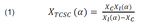
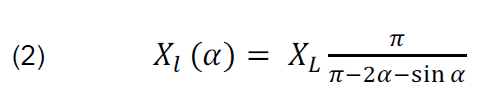
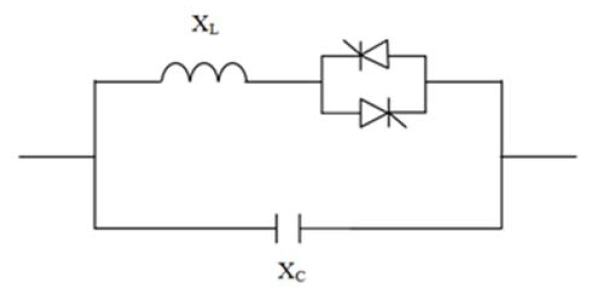
The TCSC is series type of FACTS, it consists of an inductance in series with a thyristor valve, shunted by capacitor, as shown on figure 1 [13],[14].
The impedance of TCSC can be given as following:
..
where: α : The firing angle, XL: The reactance of the inductor, XC:is the reactance of the capacitor, Xl is the effective reactance of the inductor at firing
Fig.1. Structure of TCSC
Static Var compensator
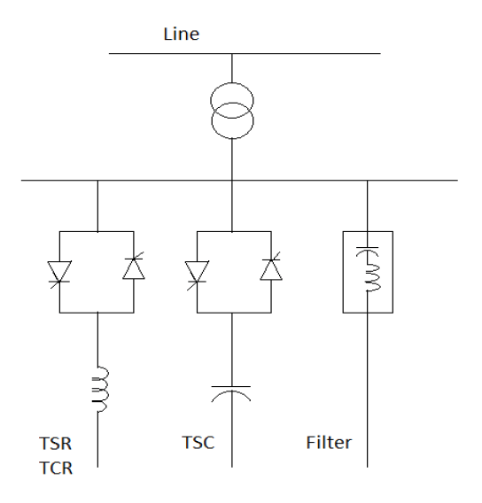
SVCs are a shunted type of FACTS controller and is a Static Var absorber or generator whose output is adjusted to exchange inductive or capacitive current to maintain the bus voltage. SVCs consist shunt reactors and capacitors,[15] which are controlled by thyristors as shown in the figure 2.
Fig.2. Structure of Static Var compensator
The main objectives of SVC are to increase the stability limit of the power system, to decrease voltage fluctuations during load variations and to limit over voltages due to large disturbances.[16] [17]
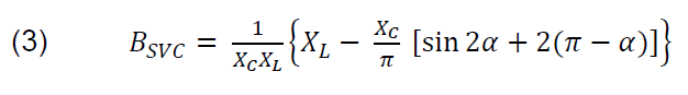
The SVC equivalent susceptance is,
.
Suppose the SVC is installed at bus k , the reactive power which injected by SVC can be describe as equation following :
.
Wind turbine generator
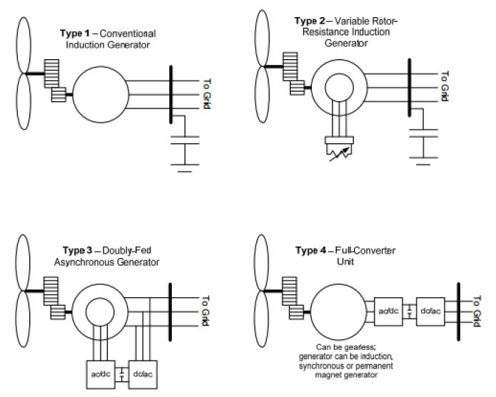
Wind power is the use of air flow through wind turbines, which convert mechanical energy to electrical energy. Today, there are several different concepts of wind turbine generator as shown in figure 3, this classification based on their connection with network, the most commonly of the new models are types 3 and 4 (USA and oversea). However, many users of type 1 and 2 in-services around the world. [18],[19].
Fig.3.Different concepts of wind turbine generator. [20]
The Power Transfer Distribution Factor
The Power transfer distribution factor shows the sensitivity of the flow on line to a transfer of power between two buses i to j, it means the change of real power in a branch flow for a 1 MW exchange between two buses [21],[22]. It shows by the following expression:
.
This method used for optimal location of TCSC and the TCSC must be placed in most sensitivity line.
where: m– line index, k – bus where power is injected, l – bus where power is taken out, Δfm – change in megawatt power flow on line m when a power transfer of ΔPk to l is made between k and l. ΔPk to l – power transferred from bus k to bus l.
The sensitivity of voltage
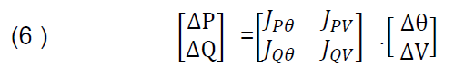
The sensitivity of voltage model was developed by Newton-Raphson method, power flow equation is given as
.
ΔP: the change in the real power, ΔQ: the change in reactive power, ΔV and Δδ are the deviations in bus Voltage magnitude and angle.
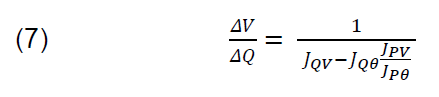
To get voltage expressed dV/dQ , the ΔP must assumed to be zero, the final expressed of dV/dQ can be written as:
.
The equation 7 is a sensitivity of voltage to an injection of reactive power at a bus has on various parameters. The SVC device can enhance the voltage stability by injected or absorbed reactive power, the voltage sensitivity used for optimal location of the SVC devices [12].
Results and discussion
In this part, we are used electrical network transmission ( IEEE 14 bus system [23].) for applied the two precedent methods of optimal location of SVC and TCSC ,in different cases of studies .
The steps of simulation are:
• Find the optimal location of FACTS ( TCSC and SVC) . • Placed FACTS in optimal location and compared the results with and without FACTS. • Injected a wind generation and compared the results with and without FACTS.
The parameters of wind generator are as following:
Type of Turbine: type 3 (machine model: GEWTG, Exciter model: EXWTGE, Governor model: WNTDGE) . The generator at bus 3 will be modelled using a GEWTG Machine, which models a 30 MW aggregation of GE 1.5 MW DFIGs (Doubly-fed induction generators). It will be equivalent 20 generators of 1,5 MW DFIGs. We replaced the generator of the bus 3 by wind turbine. Then we will find the best location of the TCSC.
Optimal location of TCSC
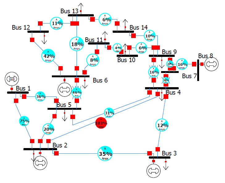
The IEEE 14 bus system drew by power world simulator, the lines don’t have limits, it observed different limit for each line , such as the highest limit could be seen in the line 4-2 (103 %) , this value indicated the line couldn’t supported transferred power (MW/MVAR) , it mean the line 2-4 overloaded. As show in the figure 4.
Suppose the line 2-4 is overloaded (103%). The main goal of this simulation is solved the overloaded. Using the optimal location of TCSC.
Fig.4. IEEE 14 bus without TCSC
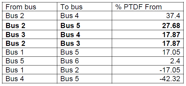
We Suppose the line 2-4 is overloaded (103%) as shown in figure 3, we use the PTDF to find the optimal location of TCSC, for solving the overloaded problems. the results of PTDF show at flowing table:
Table 1. PTDF when line 2-4 overloaded
.
We use the PTDF to find the optimal location of TCSC, for solving the overloaded problems. The results of PTDF are in the table 1
The PTDF of each line when line 2-4 was overloaded. it presented on the table 1, it observed that the most sensitivity lines were the lines 2-4 and 2-5, 37.4% , 27.68% respectively the lines 3-4 and 2-3 had the same sensitivity with 17,87 % it mean same parameters.
Before we place TCSC for each case, we must determinate the total impedance of line. Suppose the compensation is 70% , we can find the values of total impedance (X_(total)) of Xline by equation 8.
.
XTCSC = 70% Xline or XTCSC = 0.7 Xline So Xtotal = Xline – 0.7 Xline = 0.3Xline
New impedance of each line can be given as following:
Xtotal(2-5) = 0.173880 x 0.3 = 0.052164 pu Xtotal(3-4) = 0.171030 x 0.3 = 0.051309 pu Xtotal(2-3) = 0.197970 x 0.3 = 0.059391 pu
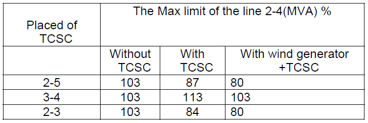
Table 2. The overloaded of line 2-4 after installing TCSC and wind generator
.
From the table 2, it is indicated the overloaded of line 2-4, after placed TCSC, and TCSC with wind generator together, the two cases explain as following:
Case one, optimal location of TCSC without wind generator:
1) TCSC in line 2-5 : After installed the TCSC in the line 2-5, it observed that, the overload of the line 2-4 decreased from 103% to 87% and creased from 75% to 80 % on the line 1-2. The TCSC reduced the overload on the line 2-4.
2) TCSC in line 3-4: When installed the TCSC in the line 3-4, it observed that the overload of the line 2-4 increased from 103% to 113 %. it indicated that not optimal location of TCSC.
3) TCSC in line 2-3: The TCSC installed on the line 2-3, it observed that the overload of the line 2-4 decreased from 103% to 84% . The TCSC reduced the overload on the line 2-4.
Case two, optimal location of TCSC with wind generator:
1)TCSC in line 2-5 and wind generator at bus 3: When we place the TCSC in the line 2-5 in presence of Wind generator placed on bus 3, the overload is decreased from 103% to 80%, it was better result compared with to install WG. The Wind Generator could be playing function of generator and system of protection.
2)TCSC in line 2-3 and wind generator at bus 3: if the TCSC is placed in the line 2-3, it removed the overload present in line 2-4 from 103% to 80%, the Wind generator was produced the active and reactive power which missed by the power system, the produced power relieved the stability of the power system.
3) TCSC in line 3-4 and wind generator at bus 3: if the TCSC is placed in the line 3-4 and wind generator installed on bus 3 , it noticed that the overload present in line 2-4 increased to 103%, according to the previous result, this line was not the optimal location of TCSC, but compared with last result the overload decreased by 10 % , from 113% to 103 % .
We can conclude that the TCSC and the wind generator can improve the power flow in the network. In our example, they suppress the overload in the line 2-4.
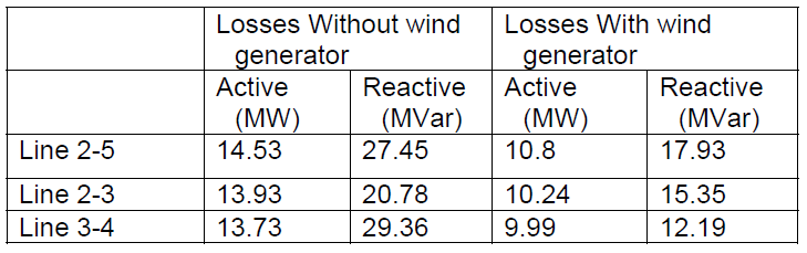
Table 3. The power loss with and without generator wind
.
The table 3 shows the active and reactive power loss with and without generator wind.
1)The total of active power loss with wind generator decreased for three cases, if TCSC placed in line 2-5 , it noticed that the total active loss minimized almost 3,73 MW , When TCSC placed in line 2-3 as shown in figure 11 the total of active power loss minimized by 3.69 Mw . Finally, The TCSC placed in line 3-4 the active power loss decreased by 3.74 Mw .
From the results, it observed the most reduced loss active power when TCSC installed in 3-4 . But this line was not the optimal location, because the overload did not removed on the line 2-4 .
The wind generator could be reduced the active power loss.
2)The total of reactive power loss with wind generator decreased for three cases, if TCSC placed in line 2-5 , it noticed that the total active loss minimized almost 9,52 Mvar , When TCSC placed in line 2-3 the total of reactive power loss minimized by 5,43 Mvar . Finally, The TCSC placed in line 3-4 the reactive power loss decreased by 17,17 Mvar .
From the results show in the table 2, it observed the most reduced loss reactive power when TCSC installed in 3-4 . But this line was not the optimal location, because the overload did not removed on the line 2-4 . The wind generator could be reduced the reactive power loss.
Optimal location of SVC
In this section, we used the same power system (14 IEEE bus system) , in this case we try used shunt type of FACTS ( SVC ) for controlling the voltage , we remember that the limit of voltage used in this simulation is ±10%.
For example:
If bus 1 has more or less 10% than it’s voltage (drop voltage or overvoltage) , we can say , that is risk ,we should use protection devices.
Table 4. Voltage profile of IEEE 14 bus in de base case
.
From the result of voltage profile which indicates in table 4 , it is noticed that most voltage of buses is between 1.06 pu and 0.92962 pu , however there are three critical buses, which are bus 12 (0.84036 pu) , bus 13(0.85519 pu) and bus 14 (0.8926 pu) .
We have just drop voltage in three buses, there is not overvoltage.
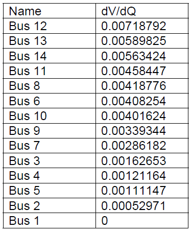
The voltage sensitivity factor used to install the SVC in the optimal placement in the power system, where the SVC should be placed in most sensitivity bus.
Table 5. Voltage profile of IEEE 14 bus in de base case
.
Table 5 shows the voltage sensitivity when we injected a reactive power. We can see different values, 0 in the slack bus (because the slack-bus has constant voltage) . The most sensitivity bus is bus 12 (0.00718792). If the SVC is installed in this bus, it will inject a reactive power which can be help to improve the voltage at the critical buses.
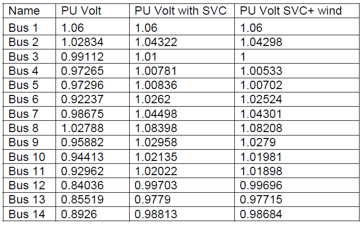
Table 6. Compared voltage magnitude for three cases
.
From the result after installing SVC at bus 12 as shown in table 6 , the voltage is improved for all buses than the base case , almost the voltage is more than 1 pu just for the critical buses improve from 0.84036 pu to 0,99703 pu at bus 12 , from 0,85519 pu to 0.9779pu at bus 13 and from 0.8926 pu to 0.98684 pu at bus 14. The slack-bus always has constant voltage.
We are noticed that the reactive power injected by SVC in bus 12 is 29.6 MVar .
The SVC is used to limit the transfer of reactive power for reduce the drop voltage. The optimal location of SVC is very important for improving the security of power system. When the SVC placed at bus 12 and changed the generator at bus 3 by wind generator, it can see that the reduction of voltage with small value of each bus , because of the variation of frequency due to the variation of speed of turbine generator.
Conclusion
This paper presents new methods for the optimal location of FACTS. The proposed method is the power transfer distribution factor used for TCSC and sensitivity voltage for SVC. We conclude, the wind generator permits to enhance the function of TCSC and SVC. As result, the active and reactive loss is decreased after injected the wind generator. The install of FACTS (TCSC, SVC) and wind generator simultaneously can be economically.
REFERENCES
[1] A. N. L. Sayyed., P. M. Gadge , Sheikh R.U., “Contingency Analysis and Improvement of Power System Security by locating Series FACTS Devices TCSC and TCPAR at Optimal Location, ” IOSR-JEEE, 2014 , p. 19-27. [2] J. Navani, M. Goyal, , S. Sapra, “Optimal Placement of TCSC and UPFC for Enhancement of Steady State Security in Power System, ” International Journal of Advances in Engineering Science and Technology, 1, 2013 , pp. 122-129, 2013. [3] S. Singh, “Location of FACTS devices for enhancing power systems’ security, ” in Power Engineering, 2001. LESCOPE’01. 2001 Large Engineering Systems Conference on, 2001. [4] Wind power by country, [online], Available at: https://en.wikipedia.org [5] Thanh Long Duong, Yao JianGang , VietAnh Truong , A new method for secured optimal power flow under normal and network contingencies via optimal location of TCSC, Electrical Power and Energy Systems journal , 53, 2013. [6] Madhura Gad, Prachi Shinde, S.U.Kulkarni ,“ Optimal ocation of TCSC by Sensitivity Methods”, International Journal Of Computational Engineering Research, Vol. 2 Issue. 6,pp 162-168,2013. [7] Ghamgeen I. Rashed , Yuanzhang Sun , H. I. Shaheen, Optimal Location and Parameter Setting of TCSC for Loss Minimization Based on Differential Evolution and Genetic Algorithm , International Conference on Medical Physics and Biomedical Engineering, Physics Procedia 33 1864 – 1878. (2012) [8] P. S. Vaidya and V. P. Rajderkar, Enhancing Power System Security by Proper Placement of Thyristor Controlled Series Compensator (TCSC), International Journal of Engineering and Technology, 4, 5, October 2012. [9] Darko Šošić, Ivan Škokljev, Nemanja Pokimica, Features of Power Transfer Distribution Coefficients in power System Networks , INFOTEH-JAHORINA ,13, pp. 86 – 90 (March 2014). [10] Chong Suk Song, Chang Hyun Park, Minhan Yoon & Gilsoo Jang , Implementation of PTDFs and LODFs for Power System Security , Journal of International Council on Electrical Engineering, 1, 1, pp. 49-53, 2011. [11] Henrik Ronellenfitsch, Marc Timme, Dirk Witthaut, A Dual Method for Computing Power Transfer Distribution Factors, JOURNAL OF L ATEX CLASS FILES, 13, 9, SEPTEMBER 2014. [12] Jitendra Singh Bhadoriya , Chandra Kumar Daheriya,“An Analysis of Different Methodology for Evaluating Voltage Sensitivity”, International Journal of Advanced Research in Electrical, Electronics and Instrumentation Engineering, vol.3, no. 9,pp 12239 – 12246,September 2014 [13] S.V. Jethani ,V.P. Rajderkar, “Sensitivity based optimal location of TCSC for improvement of power system security, ” International Journal of Research in Engineering and Technology, vol. 3, 2014, pp.121-124. [14] J. Srinivasa Rao , J. Amarnath , “Enhancement of Transient Stability in a Deregulated Power System using Facts Devices, ” Global Journal of Research In Engineering, vol. 14, 2014. [15] A. Edris, R. Adapa, M.H. Baker, L. Bohmann, K. Clark, K. Habashi, L. Gyugyi, J. Lemay, A. Mehraban, A.K. Myers, J. Reeve, F. Sener, D.R. Torgerson, R.R. Wood,“Proposed Terms and Definitions for Flexible AC Transmission System (FACTS)”, IEEE Transactions on Power Delivery, vol.12, no. 4,pp 1848-1853, October 1997. [16] Ryan.M, High-Voltage Engineering and Testing ,3rd ed, Institution of Engineering and Technology. 2013. [17] Padmavathi S.V., Sahu S.K., Todoran G., Jayalaxmi A., “Modeling and simulation of static var compensator to enhance the power system security”, in: Proceedings of the International Conference “ Postgraduate Research in Microelectronics and Electronics (PrimeAsia)”, Visakhapatnam, India, 19-21 Dec. 2013 , IEEE,06 February 2014, pp. 52-55. [18] Working Group Joint Report – WECC Renewable Energy Modeling Task Force & IEEE Working Group on Dynamic Performance of Wind Power Generation, Generic Stability Models for Type 3 & 4 Wind Turbine Generators for WECC, International conference of IEEE Power & Energy Society General Meeting, Vancouver, BC, Canada, 2013. [19] Jens Fortmann , Modeling of Wind Turbines with Doubly Fed Generator System , Springer Fachmedien Wiesbaden, Germany,2014, pp 3-5. [20] EPRI, “Proposed Changes to the WECC WT4 Generic Model for Type 4 Wind Turbine Generators”, Prepared under Subcontract No. NFT-1-11342-01 with NREL, Issued to WECC REMTF and IEC TC88 WG27 12/16/11; (last revised 1/23/13).[Online].Available:https://www.wecc.biz/Reliability/Report_on_WT4_Model_Description_PP012313.pdf. [21] Ravi Kumar, S. C. Gupta and Baseem Khan , Power Transfer Distribution Factor Estimate Using DC Load Flow Method, International Journal of Advanced Electrical and Electronics Engineering (IJAEEE),2, 6, pp. 155-159( 2013). [22] Allen J. Wood, Bruce F. Wollenberg, and Gerald B, Power Generation, Operation and Control 3 thrd edition, John Wiley & Sons, Inc., Hoboken, New Jersey . 2013. [23] http://icseg.iti.illinois.edu/ieee-14-bus-system/ last update 7 may 2014.
Authors: PhD student Messaoud Zobeidi , Department of electrical Engineering laboratory of ICEPS, Djillali Liabes Universiy, Sidi-Bel-Abbes, messoud91@yahoo.fr ; Pr Fatiha Lakdja , Department of Electrical Engineering, University Saida , laboratory of ICEPS, Djillali Liabes Universiy, Sidi-Bel-Abbes , flakdja@yahoo.fr ; Dr Yamina Ahlem Gherbi , Department of electrical Engineering, USTO-MB Oran , Durable Development of Electric Power laboratory, Algeria aygherbi@yahoo.fr ; Pr Fatima Zohra Gherbi, Department of Electrical Engineering laboratories of ICEPS, Djillali Liabes Universiy , Sidi-Bel-Abbes,Algeria ,fzgherbi@yahoo.fr
Source & Publisher Item Identifier: PRZEGLĄD ELEKTROTECHNICZNY, ISSN 0033-2097, R. 96 NR 9/2020. doi:10.15199/48.2020.09.09
Published by Bukurije HOXHA1, Risto V.FILKOSKI2 , University of Prishtina “Hasan Prishtina” (1), Ss. Cyril and Methodius University, Skopje (2) ORCID: 1. 0000-0002-8890-2054; 2. 0000-0002-3743-318X
Abstract. Optimisation of the placement of wind turbines in a farm is an important stage in wind farm construction. Koznica, a mountainous terrain available for wind farms, is considered in the present work, with the aim to optimise the configuration of a park of 10 turbines. The one-year measurements carried out in the specified place of the Koznica mountain have confirmed the wind energy potential. The present work focuses on analysing how the distance between wind turbines affects the energy produced in configurations of 2, 3 and 5 diameters distance between the turbines, using a particular turbine type with predefined technical characteristics. Interaction analysis is conducted in terms of wake effect, affecting the annual output energy and wind farm efficiency, depending on the farm configuration. The wake effect here is shown as the wind speed deficit. That deficit intensity is removed from the current and previous intensity of each respective turbine. Finally, the difference between the farm organisation’s optimised form and the previous configurations is shown, emphasising the annual energy produced depending on the capacity factor.
Streszczenie. Optymalizacja rozmieszczenia turbin wiatrowych na farmie jest ważnym etapem budowy farmy wiatrowej. W niniejszej pracy uwzględniono Koznicę, górzysty teren dostępny pod farmy wiatrowe, w celu optymalizacji konfiguracji parku 10 turbin. Roczne pomiary przeprowadzone we wskazanym miejscu góry Koznica potwierdziły potencjał energetyki wiatrowej. W niniejszej pracy skupiono się na analizie wpływu odległości między turbinami wiatrowymi na energię wytwarzaną w konfiguracjach 2, 3 i 5 średnic odległości między turbinami, z wykorzystaniem określonego typu turbiny o określonych parametrach technicznych. Analiza interakcji prowadzona jest pod kątem efektu czuwania, mającego wpływ na roczną moc wyjściową i sprawność farmy wiatrowej, w zależności od konfiguracji farmy. Efekt kilwateru jest tutaj pokazany jako deficyt prędkości wiatru. Ta intensywność deficytu jest usuwana z aktualnej i poprzedniej intensywności poszczególnych turbin. Na koniec pokazano różnicę między zoptymalizowaną formą organizacji gospodarstwa a poprzednimi konfiguracjami, podkreślając roczną produkcję energii w zależności od współczynnika wydajności. (Oddziaływanie miedzy turbinami w złożonej terenowej farmie wiatrowej)
Keywords: wind turbine, capacity factor, efficiency, energy yield, complex terrain. Słowa kluczowe: farmy wiatrowe, turbiny, oddziaływanie między turbinami
Introduction
Airflow as a potential energy source is free. Air is used as the main source of energy production in wind farms and the initial assumption is that it, as an interaction fluid, will have identical energy potential for all turbines on the farm under consideration. In order for the flow of this interaction fluid not to be affected from the previous turbine to the next, it is necessary to have an optimal possible distance between the turbines. Objectively, the optimal distance is impossible to achieve to a large extent in the case of terrains such as this one that is the subject of analysis in this case. This is due to the frequent ups and downs of the hilly terrain for which the analysis is performed. Energy is a vital key to socio-economic development and economic growth [1]. Wind energy constitutes a clean and economical source to generate electricity and is suitable for countries with moderate to high wind potential [2]. Based on Global Wind Energy Council (GWEC) data’s 2018, the worldwide newly installed wind energy capacity exceeds 60 GW in 2020, distributed over about 100 countries, and it is estimated that the globally installed wind energy capacity will exceed 800 GW [3]. Wind energy has the potential to produce power for each hour of the day and in different capacities due to different wind speeds [4]. To make the most of wind energy, between the other, improvements in the design, construction and materials must be made to have the highest energy conversion efficiency [5]. Today, wind power is considered a booming sector, and wind turbine manufacturers face difficulties meeting the market demand [6]. They are manifested in different forms, such as in the construction of the rotor part of the turbine, with the addition of other units, i.e., mini turbines [7 – 9], thus creating multiple rotors. Such a method is not yet widely used and what is known is that it contributes to a significant reduction in the total cost of a wind farm. During planning a wind farm, it is necessary to assess the wind resources of the potential site [10]. The element that requires further study is the fatigue of the structure because of the turbulence generated and the problems with reduced overall efficiency for operating in this form if it is not preceded by static side analysis [11]. According to the work [12], significant problems which must be solved to support the development of wind energy are the insurance of power transmission capacity of the electricity network, balancing the energy generated by wind power plants related to the error control of forecasting, and transition of the energy system from conventional to renewable generation. In this study, a detailed description of the parameters that characterise the placement of wind turbines in a farm according to the software and analytical method is realised. Wind measurements must be as accurate as possible to achieve optimal placement of turbines in a wind farm [13]. Greater accuracy of measured data means a more extended period of measurement and collection of wind parameters at the place where the wind farm will be built. Calculations regarding the optimisation of the placement of wind turbines on the wind farm in Koznica were made through WAsP software where the change of the interaction of the turbines between themselves can be simulated and clearly understood [14], in addition to the numerical method WEST, which is more appropriate. Studies have shown a very good correlation between the data obtained from the use of the software in question and the numerical form of the simulation [15]. Installed wind energy capacity has grown from less than 20 gigawatts (GW) in 2000 to 590 GW by the end of 2018 and already provides 6% of the electricity consumed in the world [16]. By knowing the important role that renewable-energy sources play in this context, identifying suitable sites for installing renewable-energy facilities is a crucial task [17, 18]. The wind farm layout optimisation (WFLO) problem consists of finding the turbine positions that maximise the expected power production in terms of coordinates and altitude of hub height [19]. However, the effect of wind veer causing a partial yaw error over the rotor span is rarely considered. Analysis of such effects becomes increasingly important as the dimensions of the wind turbine rotors increase [20]. To estimate the energy potential when it comes to wind energy, measurements must be made on the source side, and in this case, the key data is the wind speed. Measurements are a significant part of the cost of investing in a wind farm, and it is usually attempted to simulate the interactions of the individual turbines in a wind farm through some software such as CFD [21, 22]. To help in understanding the wind farm processes, some of the widely used wind energy application programs are being used, such as WAsP, WindPro, WindFarmer, WindSim, and Windographer [23 – 25]. However, because WAsP was developed for linear, steady flow analyses, its applicability for analyses of wind flow over complex terrain is very limited. In recent years, nonlinear, unsteady flow analyses have become possible because of the rapid improvement of computers [26 – 28]. In the last part of this work, further investigations have been carried out to compare the WEST results with linear simulation WAsP. Finally, considering commercial models of a wind turbine, the wind potential has been estimated for each turbine in this park. It is important to remark that the scope of the WEST method is not to yield more accurate or exact results concerning WAsP but to be a cheaper and faster alternative for simulations, to have good results in less time. The paper takes into consideration a very detailed and unrealized analysis of the complex mountain terrain. The more contributing is the fact that in the case of installing wind turbines in our case we have a significant change in terms of altitude. The impact of such a change is negative. This is because in such a case some “fictitious tunnels” are created which are negative loads for the turbines.
Material and Methods
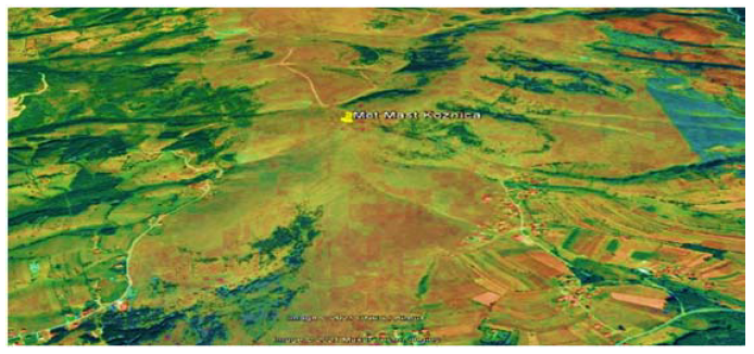
The wind farm considered in this study is in Koznice, a mountainous terrain without obstacles such as tall buildings, rocks, or trees. The considered terrain of 20 km – 20 km is considered. The determination of the coordinates is done based on the map of wind density and speed, of course, for each configuration looking to meet that condition. Figure 1 shows the specified location of Koznica, specified by its met mast.
Fig. 1. Planned Koznica wind farm
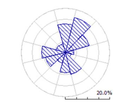
The two most essential elements that are important when analysing a potentially potential place in the field of wind energy are the intensity of the average wind speed and its direction. The wind direction in Koznica is shown in figure 2.
Fig. 2. Wind rose in Koznica
Regarding the interaction of air masses with special emphasis, it is important to take the interaction between the height referred to build the wind park and the complex terrain represented with the degree of roughness. In detail, in table 1 are presented the average speeds at heights 40, 60 and 84m.
Table. 1. Wind speed intensity
Measurement height, m
84
60
40
Average wind speed, m/s
6.16
5.85
5.64
.
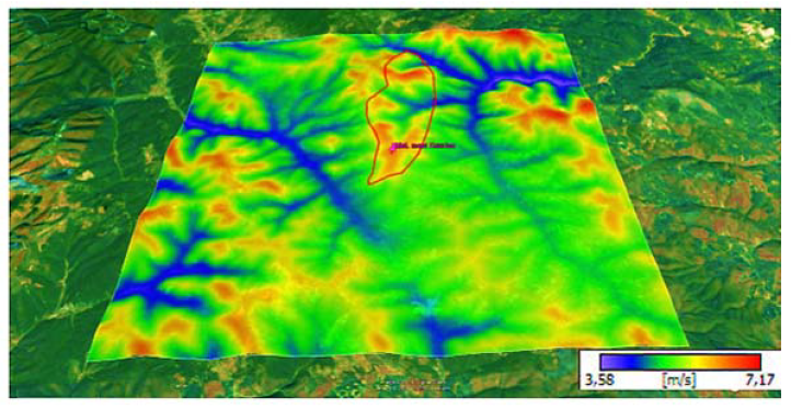
Then for energy calculation are considered 3 type of wind turbines and their number is 10. The average annual wind speed of Koznica at 84 m height above ground level is shown in Fig. 3. Maps are created using the WAsP software based on annual data from one-year measurement of met mast of location Koznica and formed digital maps of terrain orography and roughness.
Fig. 3. Average annual wind speed map of candidate region Koznica at 84 m height above ground level
Types of wind turbines considered are presented in table 2 with their technical data.
Table. 2. Main data for wind turbines used in the study, thrust coefficient, CEF, and wake decay coefficient.
WT Type
D
Pf
Zh
Wr
Wind speed, m/s
Thrust Coefficient
α
Siemens SWT-130-3.3
130
3.3
10
12.5
6.6
0.80
0.0609
Vestas V-126-3.45
126
3.45
87
20
6.9
0.785
0.0627
GE Wind GE-130-3.4
130
3.4
85
18
6.5
0.83
0.0628
.
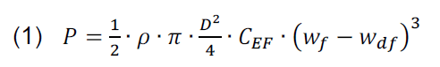
Power production modelling
To estimate the power production of WF under the wake effect, we need at the first stage to determine the power generated by each WT. There are many expressions to approximate the power curve of WT that are elaborated in detail by [29, 30]. Thus, the power production of WT is estimated as follows:
.
where CEF represents the efficiency factor expressed as follows:
.
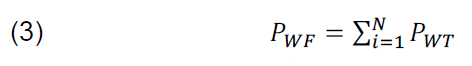
In the present study, CEF is assumed to be equal to 50%. The total power generated by WTs operating under wake effect is:
.
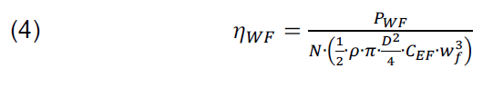
Wind farm efficiency is obtained using this equation:
.
According to Jensen wake model, the wdf – wind velocity deficit is expressed as follows:
.
Based on the Jensen model as described in figure 4 graphically, it is said that the near wake region is for 2D, Intermediate is 2-3D, and far wake > 5D distance. To see this effect then it is used for a real wind farm with real wind speed, direction and standard deviation data [31-33].
Fig. 4. Illustration of the Jensen wake model
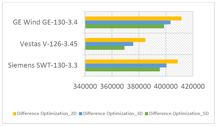
As stated initially, the difference in energy produced is not high for the best case according to Jensen and optimisation according to software and terrain taken in study [34-36]. The expression for electricity calculation is multiplied by 0.98, as a correction coefficient that brings innovation in the field of energy calculation. Difference in energy yield for each case is described in figure 5. We see that the huge amount of energy yield is for the highest distance between wind turbines, 5D.
Fig. 5. The difference in energy generation, in MWh/yr.
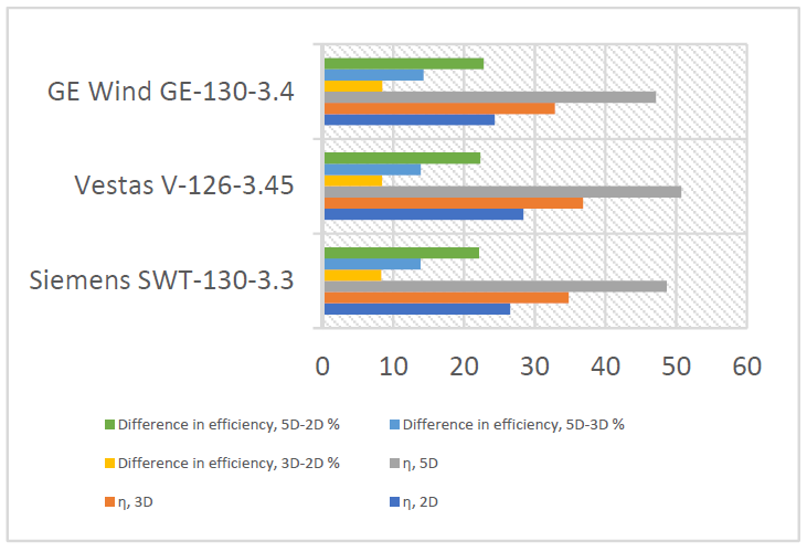
Fig. 6. Applying the Jensen model to determine the efficiency for 2D, 3D and 5D and their comparison.
The following figure shows the ratio of the largest amount of energy generated during the year for the placement of turbines at 5D distance compared to 3D and 2D cases and 3D/2D cases.
After analysing the change in the intensity of the annual energy produced within the distances then the optimisation model is formed so that we can have a clear reflection of the speed in each position of the turbines and the organising of the park, presented in figure 7.
Fig. 7. Organised wind park after optimisation of the turbines position
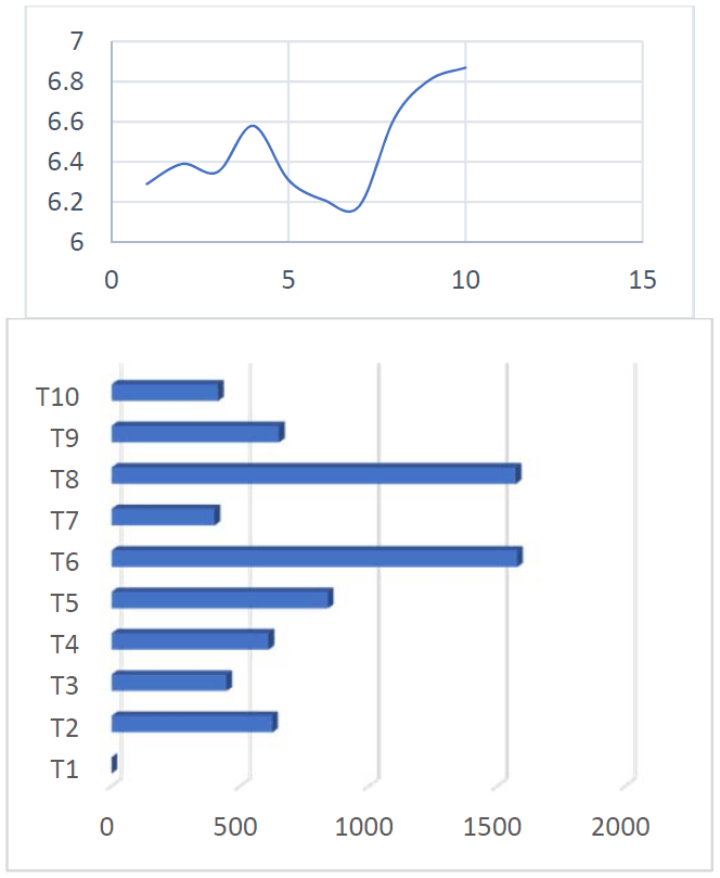
To carry out the analysis of the produced energy and efficiency it is necessary to present the data of their speed and coordinates. The data are valid for the measuring height of 110m as the average data for all turbines. The distance shown is in order from 1-2, 2-3, onwards.
Fig 8. Wind speed in m/s for each wind turbine and their distance in optimised placement in meters
From the previous figure in the optimisation configuration, we have in each turbine the speed above 6 m/s which is an indicator for the wake effect.
Conclusions
In this paper, the Jensen model has been used to study and evaluate the wind energy potential of a wind farm in Kosovo, exactly Koznica. This model allowed reconstructing the distribution of wind fields of complex territories, providing helpful information about wind farm layout optimisation. The interaction between the wind turbines is explained in terms of the wake effect created by the previous turbine in the next one. Finally, in the last part of this paper, all turbines in that windfarm have been investigated by WAsP simulations, confirming the new proposed methodology as an acceptable way for windfarm analysis. It has been shown in the paper that the wind speed deficits obtained from the Jensen wake model for a wind turbine, as a function of wind direction, depend on how we observe wakes. Results are different when considering that the deficits are observed by a point measurement, met mast, compared with those observed by a second turbine due to partial wake interaction. Moreover, the remarkable correlation between the approximated method through many calculations and that achieved by the WAsP software can be noticed, due to the linearity that accompanies them. When comparing the use of such a method with different software, we can see that we have a higher correlation with WAsP software because the modelling is linear. Future research will focus on the investigation of the structure and characteristics of the wakes originated from large wind farms under different ABL flow cases involving different land surface covers and different atmospheric stability conditions.
REFERENCES
[1] Joselin Herbert G.M., Iniyan S., Sreevalsan E., Rajapandian S., A review of wind energy technologies. Renewable and Sustainable Energy Reviews. Volume 11, Issue 6, August 2007. [2] NA. Kallioras, N.D. Lagaros, M.G. Karlaftis, P. Pachy, Optimum layout design of onshore wind farms considering stochastic loading. Adv. Eng. Softw. 88, 8–20 (2015). https://doi.org/10.1016/j.advengsoft.2015.05.002 [3] Wu, X.; Hu, W.; Huang, Q.; Chen, C.; Chen, Z.; Blaabjerg, F. Optimized Placement of Onshore Wind Farms Considering Topography. Energies 2019, 12, 2944. [4] Demolli H., Sakir A., Ecemis A., and Gokcek M., “Wind power forecasting based on daily wind speed data using machine learning algorithms,” Energy Convers. Manag., vol. 198, 2019. [5] Glassbrook, K.A., Carr, A.H., Drosnes, M.L., Oakley, T.R., Kamens, R.M., Gheewala, SH, 496 2014. Life cycle assessment and feasibility study of small wind power in Thailand. Energy for 497 Sustainable Development 22, 66–73. [6] Abbes M., Belhadj J. Development of a methodology for wind energy estimation and wind park design. JOURNAL OF RENEWABLE AND SUSTAINABLE ENERGY 6, 053103 (2014) [7] Watson, S., Moro, A., Reis, V., Baniotopoulos, C., Barth, S., Bartoli, G., Bauer, F., Boelman, E., Bosse, D., Cherubini, A., Croce, A., Fagiano, L., Fontana, M., Gambier, A., Gkoumas, K., Golightly, C., Latour, M., Jamieson, P., Kaldellis, J., and Wiser, R., Future emerging technologies in the wind power sector: A European perspective,Renewable and Sustainable Energy Reviews, Vol. 113, 10 2019, pp. 109-270. [8] Flynn, D., Rather, Z., Ardal, A., D’Arco, S., Hansen, A.D., Cutululis, N.A., Sorensen, P., Estanquiero, A., Gomez, E., Menemenlis, N. and Smith, C., 2017. Technical impacts of high penetration levels of wind power on power system stability. Wiley Interdisciplinary Reviews: Energy and Environment, 6(2), p.e216. [9] Cherubini A, Papini A, Vertechy R, Fontana M. Airborne wind energy systems: a review of the technologies. RenewSustainEnergyRev2015; 51:1461–76. [10] M. Ayala, J. Maldonado, E. Paccha, and C. Riba. Wind Power Resource Assessment in Complex Terrain: Villonaco Case-study Using Computational Fluid Dynamics Analysis. Energy Procedia, 107(September 2016):41–48, 2017. [11] Porté-Agel, F., Bastankhah, M. & Shamsoddin, S. Wind-Turbine and Wind-Farm Flows: A Review. Boundary-Layer Meteorol 174, 1– 59 (2020). https://doi.org/10.1007/s10546-019-00473-0. [12] Jonaitis, A.; Gudzius, S.; Morkvenas, A.; Azubalis, M.; Konstantinaviciute, I.; Baranauskas, A.; Ticka, V. Challenges of IntegratingWind Power Plants into the Electric Power System: Lithuanian Case. Renew. Sustain. Energy Rev. 2018, 94, 468–475. [13] Al-Abadi A, Youjin K., Ertunç. Ö, Delgado A. (2016). Turbulence impact on wind turbines: experimental investigations on a wind turbine model. Journal of Physics Conference Series 753(3). https://doi.org/10.1088/1742-6596/753/3/032046. [14] Mortensen, N. G. (2018). Wind resource assessment using the WAsP software. DTU Wind Energy. DTU Wind Energy E, No. 174 [15] Milanese M, Congedo PM, Colangelo G, et al. (2019) Numerical method for wind energy analysis in WTG sitting. Renewable Energy 136: 202–210. [16] Yusta J., Arantegui R., Measuring the internationalisation of the wind energy industry. Renewable Energy 157 (2020). Volume 157, September 2020, Pages 593-604. [17] Díaz-Cuevas, P. GIS-Based Methodology for Evaluating the Wind-Energy Potential of Territories: A Case Study from Andalusia (Spain). Energies 2018, 11, 2789. [18] Asnaz M.S.K., Yuksel B., Ergun K. (2020) Optimal Siting of Wind Turbines in a Wind Farm. In: Machado J., Özdemir N., Baleanu D. (eds) Mathematical Modelling and Optimisation of Engineering Problems. Nonlinear Systems and Complexity, vol.30 Springer, Cham. https://doi.org/10.1007/978-3-030-37062-6_6. [19] Gu H., Wang J., Irregular-shape wind farm micro-siting optimisation. Energy 57, 535-544 (2013). https://doi.org/10.1016/j.energy.2013.05.066. [20] Bardal, L. M., Sætran, L. R., and Wangsness, E.: Performance Test of a 3 MW Wind Turbine – Effects of Shear and Turbulence, Energy Proced., 80, 83–91, https://doi.org/10.1016/j.egypro.2015.11.410, 2015. [21] Tabas, D.; Fang, J.; Porté-Agel, F. Wind Energy Prediction in Highly Complex Terrain by Computational Fluid Dynamics. Energies 2019, 12, 1311. [22] Richmond, M. Antoniadis, A. Wang, L. Kolios, A. Al-Sanad, S. Parol, J. Evaluation of an offshore wind farm computational fluid dynamics model against operational site data. Ocean Engineering Volume 193, 1 December 2019, 106579. [23] Yılmaz U., Balo F., and Sua S. Simulation Framework for Wind Energy Attributes with WAsP. Procedia Computer Science. Volume 158, 2019, Pages 458-465 [24] Carvalho, D. & Rocha, A. & Santos, C. Silva & Pereira, R., 2013. “Wind resource modelling in complex terrain using different mesoscale–microscale coupling techniques,” Applied Energy, Elsevier, vol. 108(C), pages 493-504. [25] Gasset, N.; Landry, M.; Gagnon, Y. A Comparison of Wind Flow Models for Wind Resource Assessment in Wind Energy Applications. Energies 2012, 5, 4288–4322. [26] Uchida, T.; Takakuwa, S. A Large-Eddy Simulation-Based Assessment of the Risk of Wind Turbine Failures Due to Terrain-Induced Turbulence over a Wind Farm in Complex Terrain. Energies 2019, 12, 1925. [27] Mohamed B, Fadela B, Mounir K (2015) Optimisation of the wind turbines location in Kaberten wind farm in Algeria. Energy [28] CL Archer, A. Vasel-Be-Hagh, C. Yan, S. Wu, Y. Pan, J.F. Brodie, A.E. Maguire, Review and evaluation of wake loss models for wind energy applications, Appl. Energy 226 (2018) 1187e1207. [29] J. Scire, F. Robe, M. Fernaua, R. Yamartino, A User’s Guide for the CALMET Meteorological Model, Technical Report Version 5, Earth Tech Inc., Concord, MA, USA, 2000. [30] M. Milanese, L. Tornese, G. Colangelo, D. Laforgia, A. de Risi, Numerical method for wind energy analysis applied to Apulia Region, Italy, Energy 128 (2017) 1e10. [31] F. González-Longatt, P. Wall, and V. Terzija, “Wake effect in wind farm performance: Steady-state and dynamic behavior,” Renewable Energy, vol. 39, no. 1, pp. 329–338, Mar. 2012. [32] CL Archer, A. Vasel-Be-Hagh, C. Yan, S. Wu, Y. Pan, J.F. Brodie, A.E. Maguire, Review and evaluation of wake loss models for wind energy applications, Appl. Energy 226 (2018) 1187e1207. [33] Bachhal A., Vogstad K., Lal Kolhe M., Chougule A., Beyer G.H. Wake and Turbulence Analysis for Wind Turbine Layouts in an Island. ICPRE 2018. E3S Web of Conferences 64, 0 (2018). [34] Lopez-Villalobos, C.A.; Rodriguez-Hernandez, O.; Campos-Amezcua, R.; Hernandez-Cruz, G.; Jaramillo, O.A.; Mendoza, J.L. Wind Turbulence Intensity at La Ventosa, Mexico: A Comparative Study with the IEC61400 Standards. Energies 2018, 11, 3007. [35] Emejeamara, F.; Tomlin, A.; Millward-Hopkins, J. Urban wind: Characterisation of useful gust and energy capture. Renew. Energy 2015, 81, 162–172. [36] W. Miao, C. Li, G. Pavesi, J. Yang, X. Xie, Investigation of wake characteristics of a yawed HAWT and its impacts on the inline downstream wind turbine using unsteady CFD, J. Wind Eng. Ind. Aerodyn. 168 (2017) 60e71.
Authors. First author is Msc. Ass. Bukurije Hoxha, Faculty of Mechanical Engineering, University of Prishtina, street “Sunny Hill”, nn, 10000, Prishtina, e-mail: bukurije.hoxha@uni-pr.edu. Second author is Prof. Dr. Risto V. Filkoski, Faculty of Mechanical Engineering, Ss Cyril and Methodius, Rudjer Boshkovic Str. 18, 1000 Skopje, R.N. Macedonia, e-mail: risto.filkoski@mf.edu.m
Source & Publisher Item Identifier: PRZEGLĄD ELEKTROTECHNICZNY, ISSN 0033-2097, R. 98 NR 4/2022. doi:10.15199/48.2022.04.02
Published by Lidiia KOVERNIKOVA, Energy Systems Institute of the Siberian Branch of the Russian Academy of Sciences
Abstract. The paper presents the results of the analysis of harmonic parameters that were measured at the nodes of connecting railway substations to the feeding network. Traction load is nonlinear, unbalanced and stochastic. The 3-rd and 5-th harmonics are dominant in the current of the traction load. The paper shows some properties and specific features of the measured parameters of 3-rd and 5-th harmonics.
Streszczenie. W artykule zaprezentowano rezultaty analizy harmonicznych zmierzonych na węzłach połączeń podstacji kolejowych z siecią zasilającą. Sieć trakcyjna jest nieliniowa, niezrównoważona i stochastyczna. Dominują trzecia i piąta harmoniczna. (Rezultaty badania harmonicznych w sieci trakcyjnej z nieliniowym obciążeniem)
Keywords: harmonic, measurement, railway substation, traction load. Słowa kluczowe: sieć trakcyjna, harmoniczne
Introduction
Researchers have conducted very many experimental studies on harmonic conditions in the electric networks. The results of their analysis are presented in [1-11]. The studies aimed to analyse the properties and specific features of the harmonic conditions.
The presented paper gives some results of the measurements and analysis of the 3-rd and 5-th harmonic parameters at railway substations. The railway substations receive power from the 110-220 kV public networks with a frequency of 50 Hz. The feeding network is almost radial. The railway substations are distributed along the feeding network. The traction loads affect one another.
The objective of the research was to study the properties of harmonic behaviour in the network with distributed traction loads for identification of regularities. The obtained information will be used further to develop models of nodal loads for the calculation of nonsinusoidal conditions in the high voltage network.
Object of research
Electrified railway in Russia has been a source of harmonics for many years. It is very extended. In East Siberia railway occupies a special place since it is part of the Trans-Siberian railway. The railway runs across the territories with sparse population and small electric loads. At the same time the railway traffic is heavy. The time interval between trains varies from 5 to 20 minutes. The railway substations are as a rule located at a 40-60 km distance from one another, i.e. they are quite evenly distributed along the feeding network. Each section of railway between two substations receives power from two sides. The railway substation has two 40 MVA three-winding transformers. One of them is a reserve transformer. The 25 kV winding of the transformer supplies power to the traction network, whereas 6 (11) kV winding supplies power for auxiliary needs of the substation and to non-traction consumers located near the substation.
Electric locomotives receive power from the traction network. They are driven by DC engines. The engines are powered through single-phase two-pulse rectifier circuits. The rectifier circuits in the traction network cause harmonic currents. The currents of the 3-rd and 5-th harmonics have the largest value. The harmonic currents penetrate through transformers into the 110-220 kV feeding network and cause a distortion of the voltage waveform. Thus, the traction load for the feeding network is nonlinear, unbalanced and distributed. The measurements show that the voltage nonsinusoidality at the nodes of connecting railway substations to the feeding network exceeds the standard limits established in Russia [12].
The considered railway section is situated in East Siberia between the substations Mysovaya and Novoilinsky. The section contains 9 railway substations. Measurements were taken at four substations: Mysovaya, Tataurovo, Zaigraevo, Novoilinsky. For simplicity, we will denote the substations by letters M, T, Z and N respectively. The substations are located as follows: the substation T – in 126 km from the substation M, the substation Z – in 86 km from the substation T, the substation N – in 47 km from the substation Z. Arrangement of the substations relative to each other is presented in Fig. 1, where EPS – electrical power system.
Fig.1. Arrangement of the railway substations
The measurements were carried out at the points of common coupling of railway substations to the feeding network, i.e. on the high voltage side of the transformers. Measurements were performed with the aid of the device “OMSK”, which measures not only the indices of power quality but also currents, powers and other parameters. Each measurement was performed during 24 hours. The parameters were measured mainly in an interval of 1 minute. For voltage measurements the device was connected through voltage transformers to the high voltage buses. For current measurements the device was connected to current transformers installed at the inputs of high voltage transformers.
Measurements were made for three connection schemes of the railway substation:
• scheme I – traction network feeder is connected, i.e. traction network receives electric energy from the 25 kV transformer winding at the railway substation; • scheme II – traction network feeder is disconnected, i.e. traction network does not receive electric energy from the 25 kV transformer winding at the railway substation; • scheme III – passive filter in the traction network is disconnected at the railway substation.
The disconnection of the traction network feeder at either of the two substations means that the section of traction network receives electric energy only from one substation. Passive filter is tuned to absorb the 3-rd and 5-th harmonic currents. Fig. 2 shows the scheme that explains connection of transformer and circuit breakers for three schemes during measurements. The number near the circuit breaker corresponds to the number of the scheme in which the circuit breaker was switched on.
Fig.2. Connection scheme of transformer and circuit breakers
Harmonic voltages in terms of the standard requirements
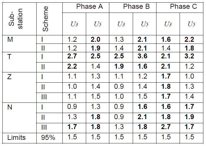
The measurements show that the standard limits [12] are considerably exceeded at 3-rd and 5-th harmonics. The values of measured harmonic voltages U3, U5, that represent the values with a probability of 95% are presented in Table 1. The values exceeding the limits are highlighted in bold.
Table 1. Measured values of U3, U5 [%]
.
Table 1 shows that:
• disconnection of traction network feeder at substation M increased insignificantly the 3-rd harmonic voltage in phase B, but decreased it in phase C, and decreased the 5-th harmonic voltage in all phases; • disconnection of traction network feeder at substation T decreased voltage at all harmonics in all phases; • disconnection of feeder at substation Z decreased the 3-rd harmonic voltage in two phases (A, B) and increased it in phase C, increased the 5-th harmonic voltage in all phases; disconnection of passive filter decreased the 3-rd harmonic voltage in all phases but increased the 5-th harmonic voltages; • disconnection of both traction network feeder and passive filter at substation N increased the voltage of the 3-rd and 5-th harmonics in all phases.
High harmonic voltages at disconnected traction network feeder testify to the fact that they are formed not only by the currents from the traction network but also by the currents drawn in the feeding network from other nonlinear loads. The decrease in the 3-rd harmonic voltage after disconnection of passive filter at substation Z is the evidence of passive filter malfunction.
The obtained results confirm that the harmonic conditions are complex, unpredictable and require thorough research before modelling them.
Active and reactive powers of the fundamental frequency
Fig. 3 shows the curves of active and reactive powers for phase B for schemes I and II for substation N. They demonstrate a typical character of change in the powers at railway substations. The curves of active and reactive powers at all substations are very similar. When the traction network feeder is connected, the powers are highly variable (Fig.3a). When traction load is disconnected, the curves of powers are ordinary (Fig.3b). The highly variable character of powers at connected traction network feeder occurs as a result of summing up the powers of a large amount of electric locomotives that operate simultaneously. In Fig. 3b a long-term decrease in powers corresponds to the night time. The power curves at connected feeder represent the total powers consumed by electric locomotives and non-traction loads. At the same time the powers of traction loads exceed the power of non-traction loads by 2-4 times.
Fig.3. Variation of P and Q for: a) scheme I, b) scheme II
The 3-rd and 5-th harmonic currents
Daily measurements of the harmonic currents represent time-series of values (Fig.4).
Fig.4. Scatter plot of the 5-rd harmonic current as function of time
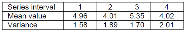
The analysis of the measured time-series of harmonic currents shows that they are non-stationary. We present the results of stationarity analysis of the time-series for the 5-th harmonic current at phase A for substation Z as an example. The time-series was divided into 4 equal intervals of 360 elements each. The mean value and variance were calculated for each interval and are presented in Table 2. The data of the Table 2 show that the mean values and variances for each interval differ in value, which gives evidence of non-stationary time-series. Analysis of the measured currents of the 3-rd and 5-th harmonics at the other substations has showed that their time-series are also non-stationary.
Table 2. Mean values and variances
.
The current curves closely resemble the above given power curves, but have a different shape. In the majority of the studied cases the values of correlation coefficients between harmonic powers and currents are low, which testifies to the weak correlation. However, in some cases there is a noticeable and high correlation, even with an opposite sign. The correlation coefficients between the active and reactive powers and the 3-rd and 5-th harmonic currents for substation N are presented in Table 3 for the sake of illustration.
Table 3. Correlation coefficients between I3, I5and P, Q
.
In scheme II the correlation coefficient in phase С equals -0.88, which is vividly shown in Fig.5. The 5-th harmonic current decreases with the active power increase and increases with its decrease. The curve of the 3-rd harmonic current changes less sharply than the curve of the 5-th harmonic current. At the same time, we clearly see the sections, where with the increase of active power the current value decreases, and vice versa. The correlation coefficient in phase C between the active power and the 3-rd harmonic currents is equal to -0.32.
Fig.5. Variation of the harmonic currents and the active power
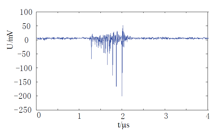
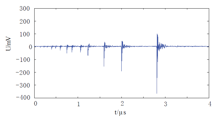
The current waveform is much distorted. It changes with time, but in general, it remains typical despite the great variety. Fig. 6 presents the oscillograms of currents for the connected feeder and disconnected feeder at substation M.
The current waveforms are much less distorted, when the feeder is disconnected.
Fig.6. Current oscillograms for: a) scheme I, b) scheme II
The analysis of harmonic composition of the traction load current shows that the value of the 3-rd harmonic current varies from 25% to 30% of the fundamental frequency current, and the value of the 5-th harmonic current is within the range from 8% to 10% of the fundamental frequency current. Table 4 presents the statistical estimates of the 3-rd and 5-th harmonic currents in one of the phases of each substation. The obtained values are of approximately the same order of magnitude at all the substations
Table 4. Statistical estimates of the 3-rd and 5-th harmonic currents
.
The curves of powers and currents demonstrate a largely probabilistic character of harmonic behaviour. Fig. 7 presents the histogram of the 3-rd harmonic current in phase А, which is measured at substation N in scheme I. This histogram has one peak.
Fig.7. Histogram of the 3-rd harmonic current
The histogram of the 5-th harmonic current in Fig. 8 has two peaks. The histograms are constructed to get an idea of the distribution function form of the measured currents of the 3-rd and 5-th harmonics. Suitable models describing the probability distribution functions of the measured harmonic parameters are to be yet chosen at a later date.
Fig.8. Histogram of the 5-th harmonic current
The properties of active and reactive components of harmonic currents are of particular interest for constructing models of non-linear loads. The histograms in Fig. 9 present the values of active and reactive components of the 5-th harmonic current. The histogram of the active current components has several faint peaks (Fig.9a). The histogram of the reactive current components (Fig.9b) has two peaks as well as the histogram of the current module in Fig. 8. The histograms of the values of active and reactive current components are the probability density functions of different forms.
Fig.9. Histograms of active a) and reactive b) components of the 5-th harmonic current
Fig. 10 presents the currents of the 3-rd harmonics in phase A of substation N for schemes I and II in the form of scatter plots on a complex plane. The diagrams make it possible to evaluate the phase angles of currents. The distributions of phase angles for 3-rd harmonic in schemes I and III differ very little from each other. The phase angles for the 3-rd harmonic are within the range from 0 to π. The phase angles for the 5-th harmonic are within the range from π/2 to 2π. Disconnection of the traction substation feeder considerably changes the phase angles. The changes take place in the scatter plots and ranges of phase angles. The phase angles for the 3-rd harmonic are distributed within the range from 0 to 2π, and for the 5-th harmonic – within the range from –π/2 to π/2.
Fig.10. Scatter plots of the 3-rd harmonic currents for: а) scheme I, b) scheme II
Analysis of the interrelation between voltages and currents of the 3-rd and 5-th harmonics The values of harmonic voltages at the points of common coupling are largely determined by the values of currents of loads connected to the node. The influence of harmonic currents passing through the substation transformers on the values of corresponding voltages is assessed by the correlation coefficients in Table 5.
Table 5. Correlation coefficients between I3, U3 and I5,U5
.
The correlation coefficients are determined for all the schemes given in Table I. The values of correlation coefficients that correspond to the noticeable and high values are shown in bold. There is a considerable linear relationship between the voltages and currents of the 3-rd and 5-th harmonics at substation Z in scheme II and of the 5-th harmonic at substation N in scheme II. In most of the other cases the relationship is weak, which indicates a strong influence of the harmonic currents of other nonlinear loads on the voltage. The harmonic voltage at the substation arises due to the effect of numerous nonlinear loads connected to the feeder.
Resonance conditions at the 3-rd and 5-th harmonics
The measurements at substation T that were made by metering device demonstrated a sharp increase in the 3-rd and 5-th harmonic voltages. Fig. 11 shows a range of measured 5-th harmonic voltages in which resonance conditions are well seen. A sharp increase in voltage occurs after the 15-th measurement. It turned out that at this moment a 44 MVAr capacitor bank was switched on at the substation of power supply organization, which is located in the area of railway substation T, to maintain the fundamental frequency voltage.
Further analysis and calculations showed that after switching the capacitor bank a resonance loop occurred between the capacitor bank and network at the 3-rd and 5-th harmonics. Before the connection of capacitor bank the input conductance at the network node at the 3-rd harmonic was inductive, whereas after the connection its value decreased almost by 4 times. At the 5-th harmonic the input conductance became capacitive but of a very low value. The capacitor bank compensated the inductive conductance of the network node. The 3-rd and 5-th harmonic conditions are unbalanced. Unbalance of voltages and currents increased after the connection of capacitor bank.
Fig.11. Change in the 5-th harmonic voltages after connection of capacitor bank
Conclusions
At all the substations, where the measurements were taken, the standard limits harmonic voltages were exceeded. The limits of the 3-rd and 5-th harmonic voltages were exceeded most frequently and to a greater degree.
Oscillograms of phase currents essentially differ from sinusoidal form when feeders of traction network are switched on. Currents are considerably unbalanced. Traction load introduces a significant probabilistic component to the harmonic behaviour in the network. The harmonic currents in the network with numerous distributed nonlinear loads are conditioned by the effect of numerous loads.
Currents of the 3-rd and 5-th harmonics represent nonstationary time-series. They are weakly correlated with fundamental frequency active powers in the scheme with connected feeders of traction network. A greater extent of correlation is observed in the schemes with disconnected passive filters. Considerable correlation occurs in the schemes with disconnected feeders of traction network. Strong correlation between harmonic currents and voltages is revealed in the schemes with disconnected feeders of traction network at all substations except for T.
Probability distributions of currents of the 3-rd and 5-th harmonics have single- and double-peaked histograms, whose forms usually differ from the normal distribution. Histograms of active and reactive current components have different forms of probability density functions.
In the general case the phase angles of currents of the 3-rd and 5-th harmonics are within the range from 0 to 2π and change at disconnection of the traction network feeder.
Connection of capacitor bank resulted in resonance conditions at the 3-rd and 5-th harmonics, which increased voltages and currents of the 3-rd and 5-th harmonics.
Acknowledgment: The work was supported by the grant of the Leading Scientific School of the RFSS НШ-1507.2012.8.
REFERENCES
[1] T.C. Shuter, H. T. Vollkommer, T.L. Kirkpatrick, A survey of harmonic levels on the American electric power distribution system, IEEE Trans. on Power Delivery, vol. 4, No. 4, October 1989, 2204-2213. [2] A.E. Emanuel, J.A.Orr, D.Cyganski, E.M.Gulachenski, A survey of harmonic voltages and currents at distribution substantions, IEEE Trans. on Power Delivery, vol. 6, No. 4, October 1991, 1883-1890. [3] A.E. Emanuel, J.A.Orr, D.Cyganski, E.M.Gulachenski, A survey of harmonic voltages and currents at the customer’s bus, IEEE Trans. on Power Delivery, vol. 8, No. 1, January 1993, 411- 421. [4] Y.J. Wang, L. Pierrat, L. Wang, Summation of harmonic currents produced by AC/DC static power converter with randomly fluctuating loads, IEEE Trans. on Power Delivery, vol. 9, No. 2, April 1994, 1129-1135. [5] A. Mansoor, W. M. Grady, A. H. Chowdhury, M. J. Samotyj, An investigation of harmonics attenuation and diversity among distributed single-phase power electronic loads, IEEE Trans. on Power Delivery, vol. 10, No. 1, January 1995, 467-473. [6] A.Cavallini, G.C.Montanari, M.Cacciari, Stochastic evaluation of harmonics at network buses, IEEE Trans. on Power Delivery, vol. 10, No. 3, July 1995, 1606-1613. [7] Chung-Hsing Hu, Chi-Jui Wu, Shih-Shong Yen, Yu-Wu Chen, Bor-An Wu, Jan-San Hwang, Survey of harmonic voltage and current at distribution substation in Northern Taiwan, IEEE Trans. on Power Delivery, vol. 12, No. 3, July 1997, 1275-1284. [8] A.Cavallini, R.Langella, A. Tesla, F. Ruggiero, Gaussian modeling of harmonic vectors in power systems, 8th International conference on Harmonics and Quality of Power, Athens, Greece, 14-16th Oct.1998, Proccedings, vol.II, 1010-1017. [9] Probabilistic Aspects Task Force of Harmonics working group Subcommittee of the Transmission and Distribution committee, Time-varying harmonics: part I – characterizing measured data, IEEE Trans. on Power Delivery, vol. 13, No. 3, July 1998, 938-944. [10] I.M.Neidawi, A.E.Emanuel, D.J.Pileggi, M.J.Corridori, R.D. Archambeault, Harmonics trend in NE USA: a preliminary survey, IEEE Trans. on Power Delivery, vol. 14, No. 4, October 1999, 1488-1494. [11] A. Ardito, S. Malgarotti, A. Prudenzi, A survey of power quality aspects at industrial customers in Italy, 17th International conference on Electricity Distribution, Barcelona, Spain, 12-15 May, 2003, Proccedings, vol.II, 1010-1017. [12] State standard R 54149-2010. Electric energy. Electromagnetic compatibility of technical equipment. Power quality limits in the public power supply systems. Moskva. Standartinform. 2012.
Authors: Ph. D. Lidiia Kovernikova, Energy System Institute SB RAS, 130, Lermontov Str., Irkutsk, 664033, Russian Federation, E-mail: kovernikova@isem.sei.irk.ru.
Source & Publisher Item Identifier: PRZEGLĄD ELEKTROTECHNICZNY, ISSN 0033-2097, R. 89 NR 11/2013
Published by Michał MAJKA, Janusz KOZAK, Electrotechnical Institute
Abstract. The superconducting fault current limiter (SFCL) is a device allowing for a more effective use of the existing power network infrastructure. The limitation of short-circuit currents by the SFCL to safe levels will result in the network elements being susceptible to smaller electrodynamic and thermal overloads. This paper presents the electrical scheme, design and numerical model of the 15 kV class SFCL prototype.
Streszczenie. Nadprzewodnikowy ogranicznik prądu zwarciowego (NOPZ) jest urządzeniem pozwalającego na lepsze wykorzystanie istniejącej infrastruktury sieciowej. Ograniczenie przez prądów zwarciowych do bezpiecznego poziomu sprawi, że elementy sieci będą narażone na mniejsze przeciążenia cieplne i elektrodynamiczne. W artykule przedstawiono schemat elektryczny, projekt i model numeryczny prototypu ogranicznika na napięcie 15 kV. (Bezrdzeniowy nadprzewodnikowy ogranicznik prądu 15 kV 140 A).
Keywords: superconductivity, superconducting fault current limiter, SFCL, numerical analysis. Słowa kluczowe: nadprzewodnictwo, nadprzewodnikowy ogranicznik prądu, SFCL, analiza numeryczna.
Introduction
The superconducting fault current limiter (SFCL) introduces minimal impedance to the power system under normal conditions and high resistance during faults, limiting short circuit current. The main duty of the SFCL is decreasing the fault current to safe level and avoid network instability. The electrodynamic forces occurring during the course of a fault current may damage the devices of the electric power system, such as transformers, generators or busbars in switching stations, within tens of milliseconds. Every such failure of an electric power network entails expensive and time-consuming repairs. Therefore, it is vital that the network’s operation be secured with a reliable protection system. A rapid increase of the resistance of a superconductor on crossing the current critical value Ic makes it possible to build reliable superconducting fault current limiters (SFCLs). SFCLs react very rapidly by limiting the first, the most dangerous, surge current during a current fault condition, thus protecting the devices of the electric power network from the dynamic effects of current faults. The SFCL responds before the first cycle peak and provides an effective means to limit excessive fault currents to safe levels without the disadvantages of conventional fault current mitigation methods.
The SFCLs provide an economic solution for protecting the devices of the electric power system against excessive short circuit currents in case of faults. The application of a SFCL leads to an increase of the allowable short-circuit power at the point of connection of new power generating sources, which is determined by the short-circuit parameters of the power network. This, in turn, will result in an increase of the capability of the power network for connecting distributed generation energy sources based on renewable energy sources. Present researches on current limiters focus on resistive type [5], inductive type [1], [2], [4], [6], [7] and limiters with a saturated core [10]. The drawback of the concept of inductive limiter with shielded core was insertion of a finite impedance in the line even during normal operation, and the large size and weight of the iron core [9]. The presented solution of a coreless construction reduces the weight of the device and the size of the primary copper winding and the voltage on the limiter during the normal operation is negligible [4].
The design of the SFCL
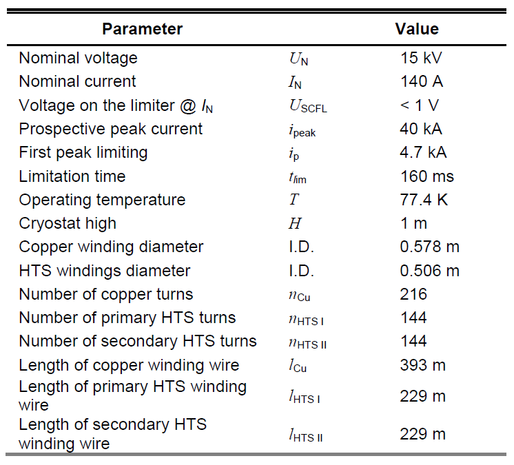
A design of a 1-phase inductive type superconducting limiter is presented in Figures 1-4. The limiter was designed to work in a 15 kV power system. Its main parameters are presented in table 1.
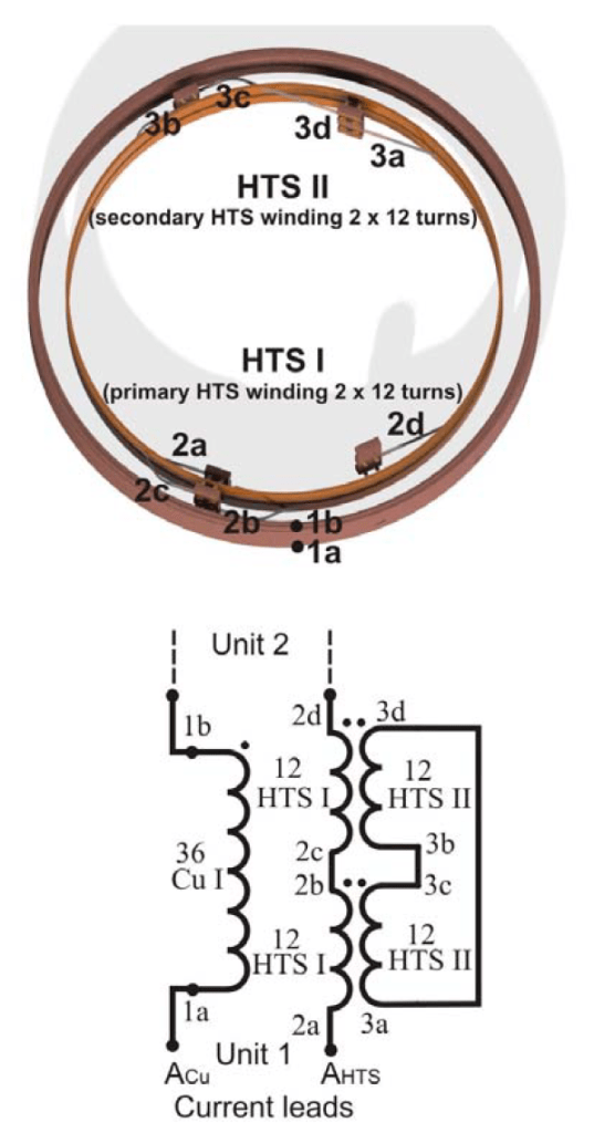
Fig. 1. Design of the SFCL (six identical units connected in series)
Fig. 2. View of one unit of the SFCL
A three-winding superconducting current limiter has two primary windings and one secondary winding [1], [4]. The primary winding, placed on the outer ring, is made of a copper wire. The second primary winding, placed in the inner ring, is made of a 2G superconducting tape. The third winding is a shorted secondary winding made of a 2G superconducting tape, placed in the inner ring.
Fig. 3. Structure cross-section of SFCL
Fig. 4. One unit electrical connections of the SFCL
The primary winding made of 2G tape is connected in parallel with the copper primary winding. All three windings are magnetically coupled. The magnetic coupling between the 2G tape windings in the inner ring is greater than the magnetic coupling between the 2G tape winding and the copper winding in the outer ring. The coupling coefficient between primary HTS and secondary HTS windings is 0.97 and between primary copper winding and secondary HTS winding is about 0.52.
Table 1. Parameters of SFCL
.
The limiter will be placed in a cryostat with an external vacuum insulation and cooled in a liquid nitrogen bath (Fig. 1). The cryostat of the limiter will be made of GFRP (Glass Fiber Reinforced Polymer). It will be fitted with four copper current leads (Fig. 1) to which the primary, both copper and HTS, windings terminals will be connected. This will allow to record the distribution of currents in these windings during short-circuit tests.
The limiter consists of six identical modules connected in series (Fig. 1 – 4), which allows to lower the voltage of the individual windings. There is 2.5 kV per one module. The superconducting tapes will be insulated with 0.025 mm thick polyimide film with a 0.040 mm silicone adhesive during the winding process. Dielectric strength of DuPont Kapton FN polyimide film is 5.9 kV.
Each module consists of two carcasses of different diameters which are made of composite materials reinforced with fibreglass. The copper winding will be wound onto an external bobbin and the superconducting windings on an internal bobbin. In each of the six modules the primary copper winding has 36 turns and is connected in parallel with two primary superconducting windings. The primary superconducting windings have 12 turns each and are connected in series. The secondary superconducting windings consist of two shorted superconducting windings, each with 12 turns. Both the primary and the secondary superconducting windings are wound onto a single bobbin in such a way that their turns are positioned one on top of the other, which provides a very good magnetic coupling between the windings and this, in turn, reduces the voltage during the SFCL’s performance in nominal conditions.
The primary copper winding will be wound using a 3 mm x 6 mm copper wire. The superconducting windings will be wound using the SF12050 superconducting tape with 2 μm silver layer and a resistance of HTS tape 0.104 Ω/m in resistive state at 77.4 K [3]. The primary and secondary superconducting windings are of the same length and have the same number of turns. A Kapton tape will be used to insulate the superconducting windings. Figure 4 represent the connections of the windings of each of the six modules.
Numerical model of SFCL
The numerical model of the limiter was developed in the “Transient Magnetic” FEM-circuit Flux2D software [8]. The geometry of the actual model of the limiter was substituted with a simplified axially symmetric geometry (Fig. 5).
Fig. 5. Simplified geometry of numerical model in Flux2D for all 6 units
Fig. 6. Electric circuit of numerical model of SFCL in Flux2D
The outer circuit of the numerical model is presented in Fig. 6. The thermal issues which occur in the windings of the limiter are included in the user subroutine written in Fortran. According to this procedure, in every step in the calculations the temperature of the limiter’s winding is determined using the energy balance, based on the present value of the current flowing through the limiter’s windings. The energy balance equation takes into account the transition of the heat from the limiter windings to the cooling liquid. After determining the current temperature of the winding, the resistance of the winding is calculated on the basis of experimentally determined R(I,T) relation for the SF12050 superconducting tape [3].
Simulations were performed for model of limiter whose parameters are presented in table 1. Thanks to the performed simulations, courses of a fault current in the circuit with and without the limiter were obtained (Fig. 7), as well as the changes of resistance and temperature of individual limiter windings during the limitation of the fault current (Fig. 9).
In the stand-by state, i.e. the first 40 ms of calculations, the superconducting windings of the limiter are in the superconducting state and a nominal current of 140 A flows through the limiter (Fig. 8). The voltage value in all models of the limiter is lower than 1 V, which results from a minor leakage reactance.
During a short-circuit lasting from 0.040 sec. to 0.200 sec., a fault current flows through the limiter. The peak value of the current in the shorted circuit ip = 40 kA was limited to 4.7 kA (Fig. 7). The course of the fault current causes the HTS windings to heat up very rapidly. The temperature of the windings increases from an initial temperature of 77.4 K to a maximum temperature Tmax which is reached at the moment of switching off of the short-circuit (Fig. 9c).
Fig. 7. Current waveforms in the circuit with and without SFCL
Fig. 8. Current waveforms in the windings of the limiter in stand-by state
Fig. 9. Numerical model – current waveforms in the windings of the limiter (a), the changes of resistance (b) and temperature of individual limiter windings (c) during the limitation of the fault current (graphs for HTS I and HTS II windings overlap).
The performed simulation shows that the temperature of the superconducting windings increases much faster than the temperature of the copper windings, and it reaches different values at the moment of switching off of the short-circuit. In designing the limiter, it was assumed that the maximum temperature of the limiter’s superconducting windings at the moment of a short-circuit occurrence would not exceed 200 K and the fault current peak value would be below 5 kA
Conclusion
The developed design in which the superconducting windings are wound simultaneously onto a single bobbin allows to obtain a very high coupling factor between the windings and minimize the leakage reactance of the limiter, which minimizes the voltage in the limiter in the stand-by state. In case of a 2-winding design in which the primary copper winding is magnetically coupled with a secondary HTS winding, there always occurs leakage reactance, which causes losses in the stand-by state. The use of a connection in parallel of a copper coil and a superconducting coil in the primary winding protects the short circuit from opening in case when the superconducting tape is damaged. The fault current limiting capability of a 3-winding limiter is determined mostly by the impedance of the copper winding coupled in parallel with the primary superconducting winding.
An analysis of the results of the numerical simulations confirmed that it is possible to build an inductive type coreless superconducting fault current limiter that will effectively limit the peak value of the fault current from 40 kA to 5 kA within 160 ms. The number of turns in the primary copper winding and the superconducting tape length in the superconducting windings must be such that the temperature of the HTS windings does not exceed the maximum allowed temperature of the superconducting tape. Due to a substantial increase of the temperature of the limiter’s HTS windings, the short circuit must be switched off by a conventional circuit breaker before the temperature of the HTS winding reaches the maximum value.
This work was supported in part by the National Centre for Research and Development under Grant UMO2012/05/B/ST8/01837.
REFERENCES
[1] Kozak J., Majka M., Janowski T., Kozak S., Wojtasiewicz G., Kondratowicz-Kucewicz B., “Tests and Performance Analysis of Coreless Inductive HTS Fault Current Limiters”, IEEE Trans. Appl. Supercond., 21 (2011), No. 3, 1303 – 1306. [2] Naeckel O., Noe M., “Design and Test of an Air Coil Superconducting Fault Current Limiter Demonstrator ”, IEEE Trans. Appl. Supercond., 24 (2014), No. 3, article nr 5601605. [3] Czerwinski D., Jaroszynski L., Majka M., Kozak J., “Analysis of Alternating Overcurrent Response of 2G HTS Tape for SFCL”, IEEE Trans. Appl. Supercond., 24 (2014), No. 3, 5600104 [4] Kozak J., Majka M., Kozak S., Janowski T., „Design and Tests of Coreless Inductive Superconducting Fault Current Limiter”, IEEE Trans. Appl. Supercond., 22 (2012), No. 3, 5601804 [5] Kozak J., Majka M., Kozak S., Janowski T., „Comparison of Inductive and Resistive SFCL”, IEEE Trans. Appl. Supercond., 23 (2013), No. 3, 5600604 [6] Heydari H., Sharifi R., “Three-Dimensional Pareto-Optimal Design of Inductive Superconducting Fault Current Limiters”, IEEE Trans. Appl. Supercond., 20 (2010), No. 5, 2301 – 2311 [7] Naeckel O., Noe M., “Conceptual Design Study of an Air Coil Fault Current Limiter ”, IEEE Trans. Appl. Supercond., 23 (2013), No. 3, article nr 5602404. [8] de Sousa W.T.B., Nackel O., Noe M., “Transient Simulations of an Air-Coil SFCL”, IEEE Trans. Appl. Supercond., 24 (2014), article nr 5601807. [9] Janowski T, Wojtasiewicz G., Kondratowicz-Kucewicz B., Kozak S., Kozak J., Majka M., „Superconducting Winding for Inductive Type SFCL Made of HTS Tape With Increased Resistivity”, IEEE Trans. Appl. Supercond., vol. 19, issue: 3, pp. 1884 – 1887, 2009. [10] Hong H., Su B., Niu G.J., Cui J.B., B. Tian, Q., Wang L.Z., Wang Z.H., Zhang K., Xin Y., “Design, Fabrication, and Operation of the Cryogenic System for a 220 kV/300 MVA Saturated Iron-Core Superconducting Fault Current Limiter”, IEEE Trans. Appl. Supercond., vol. 24, issue: 5, article nr 9002204, 2014.
Authors: dr inż. Michał Majka, Instytut Elektrotechniki, ul. Pożaryskiego 28, 04-703 Warszawa, E-mail: m.majka@iel.waw.pl; dr hab. inż. Janusz Kozak, Instytut Elektrotechniki, ul. Pożaryskiego 28, 04-703 Warszawa, E-mail: j.kozaki@iel.waw.pl
Source & Publisher Item Identifier: PRZEGLĄD ELEKTROTECHNICZNY, ISSN 0033-2097, R. 92 NR 7/2016. doi:10.15199/48.2016.07.06
APPLICATION NOTE IEEE STD 519 – 2022 UPDATE_HARMONIC STANDARD
*Mirus’ SOLVTM simulation software1
IEEE Standard for Harmonic Control in Electric Power Systems (IEEE Std 519-2022), is a highly recognized and referenced standard, and has been updated in 2022 from its prior 2014 version. The purpose of the standard is to establish goals for the design of electrical systems that include both linear and nonlinear loads2.
Please note that Mirus is not responsible for any misinterpretation of the standard, and the following notes are Mirus’ interpretation only. The more significant changes are shown in bold:
• Title Change: ‘Recommended Practice and Requirements’ changed to ‘Standard’. Although the title has removed the word ‘recommended’, the fact is that the use of IEEE Std 519 still remains wholly voluntary. Several other verbage simplifications have been made throughout the document as effort to simplify and help avoid misinterpretation of the standard.
• The introduction mentions that users should not add equipment that affects the impedance characteristic in such a way that voltage distortions are increased. The word ‘passive’ has now been removed from this description, so now we can interpret that ALL equipment should be considered to meet this criteria.
• Scope added to include Inverter-Based Resource (IBR) and/or Distributed Energy Resource (DER) installations which direct the User to IEEE Std 15473 or IEEE Std 28004 for current distortion limits if the combined site rated generation is >=10% of the annual average load demand. A Decision Tree has been provided as Figure 1 in the standard to determine whether IEEE Std 519 current limits apply at the PCC.
Figure 1: Decision tree for applying current distortion limits at PCC2
• Additional note in the scope that the limits given in this document are justifiable only at the PCC, and not intended to be used for the evaluation of equipment. This was always the intent of the standard, but some additional clarification has been included. Although IEEE Std 519 does not specify limits on individual equipment, Mirus accepts that some engineers/specifications may choose to apply specify limits on certain non-linear loads. This strategy can be used to ensure compliance at the PCC provided there is no system resonance conditions at the residual harmonics and/or all nonlinear loads contributing to the distortion at the PCC have been considered.
• Additional clarity provided for the ‘maximum demand load current’ to clarify how it is calculated by the max 15 or 30min demand, and what to do if 12 months of data is not available. If not available, then it shall be based on the projected 15- or 30-min demand. Previously it was not clear what should be done for new installations or when 12 months of data was not available.
• Harmonic measurements for IEEE 519 evaluation are required to be made up to the 50th using Class A instruments. Class S would only require measurement up to the 40th harmonic. This clarification may help those looking to use or purchase a power analyzer.
• Even-order harmonic current limits have been relaxed. Previously all even-order harmonics were limited to 25% of the individual harmonic limits as provided in the current limit tables. Now the current harmonic limits have been increased for even harmonics.
For h<=6 -> Limits have increased from 25% to 50% of the individual limits shown in the tables.
For h>6 -> Limits have increased from 25% to 100% of the individual limits shown in the tables.
Even-order harmonics are not desirable on power systems, and their appearance can indicate asymmetry between the positive and negative halves of the waveform. Perhaps it was felt that these increases were required due to the larger numbers of IBR, AFE drive and active filters, which may result in some levels of even order harmonics that may not have always been meeting the more stringent even-order harmonic limits in the previous 2014 standard.
• Annex A. Significant changes to the Interharmonic Voltage Limits and Rationale. The standard mentions that more detail can be provided by referencing a paper by Drapela, et al [B3] “Issues and Challenges Related to Interharmonic Distortion Limits”, 2020. 5
Interharmonics can be difficult to address when dealing with active devices such as IBR, AFE Drives and active filters because they can often generate interharmonics. Passive filters typically treat harmonics over a frequency range so both harmonic and interharmonic frequencies are usually addressed.
The recommended limits (not prescriptive) are based on analysis of the sensitivity of lighting equipment (LEDs) to prevent flicker, and also more strict limits required on sensitive non-lighting equipment. Appropriate limits should be based on specific needs (local, country, conditions, etc.).
References
1. SOLVTM Software Registration and Download, https://www.mirusinternational.com/register.php 2. IEEE Std 519-2022, IEEE Standard for Harmonic Control in Electric Power Systems. 3. IEEE Std 1547-2018, IEEE Standard for Interconnection and Interoperability of Distributed Energy Resources with Associated Electric Power Systems Interfaces. 4. IEEE Std 2800-2022, IEEE Standard for Interconnection and Interoperability of Inverter-Based Resources (IBR) Interconnecting with Associated Transmission Electric Power Systems. 5. Drapela, J., M. Halpin, R. Langella, J. Meyer, D. Mueller, H. Sharma, A. Testa, N. Watson and D. Zech, “Issues and Challenges Related to Interharmonic Distortion Limits,” 2020 19th International Conference on Harmonics and Quality of Power (ICHQP), Dubai, United Arab Emirates, 2020, pp. 1–6, doi: 10.1109/ICHQP46026.2020.9177933.
Published by Electrotek Concepts, Inc., PQSoft Case Study: IEEE 519 Compliance, Document ID: PQS0321, Date: October 10, 2003.
Abstract: IEEE Standard 519-1992 is a standard that addresses the need for limiting the harmonic current a customer injects onto the utility system. It also protects the customer by specifying maximum harmonic voltage distortion levels that utilities can supply.
The installation of a 3% choke on each drive and a 150kVAr harmonic filter on the bus reduced the harmonic currents to acceptable values.
This case presents the evaluation of IEEE 519 compliance for an industrial facility supplying adjustable-speed drives.
PROBLEM STATEMENT
A wastewater treatment plant is installing five (5) 100 HP pulse width modulation (PWM) adjustable-speed drives (ASDs). The utility has specified that IEEE 519 current limits must be met.
The combined drive load has the following characteristics:
Drive Rating: 500 HP Bus Voltage: 480 V Fundamental Current: 600 A
SYSTEM CONFIGUATION
Figure 1 illustrates the oneline diagram used for the analysis of IEEE 519 compliance.
IEEE Standard 519-1992 is a standard that addresses the need for limiting the harmonic current a customer injects onto the utility system. It also protects the customer by specifying maximum harmonic voltage distortion levels that utilities can supply. The standard should be used for guidance in the design of power systems with nonlinear loads. Table 1 summarizes the current requirements.
Table 1 – Current Limits for Individual Customers (120V – 69kV)
.
where:
SCR: ratio of the short circuit current at the point of common coupling to the maximum average demand load current (Isc/Iload)
TDD: Total Demand Distortion, current distortion in percent of the maximum average demand load current
IEEE 519 defines the point of common coupling (PCC) as: A point of metering or any point as long as both the utility and the customer can either access the point for direct measurement of the harmonic indices meaningful to both or estimate the harmonic indices at a point of interference (POI) through mutually agreeable methods.
LOAD CURRENT EVALUATION
Table 2 summarizes the current requirements for the initial case with no harmonic current reduction. This evaluation illustrates the need for harmonic current mitigation. As can be seen in the table, most of the individual harmonic currents and the total demand distortion are exceeded for this case. In addition, the bus voltage distortion of 9.8% is higher than the generally accepted limit of 5%.
The harmonic voltages are determined by multiplying the current injection times the impedance at each harmonic. The maximum average demand load current is used to scale the individual harmonic currents for comparison with the specified limits.
Table 2 – Evaluation of Current Limits for Base Case
.
Note: Id is based on the average maximum demand load current
MITIGATION TECHNIQUES
Several techniques for reducing the harmonic current were evaluated:
1. Installation of a 3% choke on each drive (refer to Figure 1 for new current waveform) 2. Installation of a 3% choke and a 30kVAr, 5th harmonic filter on each drive 3. Installation of a 3% choke on each drive and a 150kVAr, 5th harmonic filter on the 480 volt bus
Table 3 summarizes the results from the computer simulations.
Table 3 – Evaluation of Current Limits for Various Solutions
.
SUMMARY
IEEE Standard 519-1992 is a standard that addresses the need for limiting the harmonic current a customer injects onto the utility system. It also protects the customer by specifying maximum harmonic voltage distortion levels that utilities can supply. The installation of a 3% choke on each drive and a 150kVAr harmonic filter on the bus reduced the harmonic currents to acceptable values.
REFERENCES
IEEE Recommended Practice for Electric Power Distribution for Industrial Plants (IEEE Red Book, Std 141-1986), October 1986, IEEE, ISBN: 0471856878 IEEE Recommended Practice for Industrial and Commercial Power Systems Analysis (IEEE Brown Book, Std 399-1990), December 1990, IEEE, ISBN: 1559370440
RELATED STANDARDS IEEE Standard 519-1992
GLOSSARY AND ACRONYMS ASD: Adjustable-Speed Drive DPF: Displacement Power Factor PCC: Point of Common Coupling PF: Power Factor PWM: Pulse Width Modulation POI: Point of Interference SCR: Short Circuit Ration TDD: Total Demand Distortion THD: Total Harmonic Distortion TPF: True Power Factor
Published by JUNHAO LI1, YANMING LI1, GUOLI WANG2, Martin D. JUDD3, State Key Laboratory of Electrical Insulation and Power Equipment, Xi’an Jiaotong University (1) Electric Power Research Institute of China South Grid (2) Institute for Energy and Environment, Department of Electronic and Electrical Engineering, University of Strathclyde (3)
Abstract. Partial discharge (PD) detection is a technique widely used for high voltage equipment insulation condition assessment. In such applications, an understanding of PD mechanisms, characteristics and development processes is important. In this paper, PD characteristics of three typical transformer oils, aged to different degrees, are examined under AC conditions, using a needle-to-plane electrode system. The PD activity in transformer oil is confirmed as appearing in pulse burst form. Pulse burst characteristics recorded in the study show that the transferred electric charge per PD pulse burst increases with the degree of aging. This increase is accompanied by an increase in the number of discrete PD pulses and by a decrease in cavity formation time. The experimental results of cavity discharge in differently aged transformer oils are discussed and their characteristics are explained in terms of the charge exchange mechanism.
Streszczenie. Przedstawiono charakterystyki wyładowania niezupełnego w trzech typowych olejach transformatorowych o rożnym stopniu starzenia przy zasilaniu napięciem przemiennym. Stwierdzono, że impulsy wyładowania zależą od stopnia starzenia. (Charakterystyki impulsów wyładowania niezupełnego w oleju transformatorowym o różnym stopniu starzenia)
Keywords: partial discharges; oil insulation; pre-breakdown; PD pulse burst; power transformer. Słowa kluczowe: wyładowanie niezupełne, transformatory mocy, izolacja olejowa.
1. Introduction
Transformers are key and widespread components of the power network. Mineral insulating oil plays a major role in power transformers, acting both as insulation and coolant. The presence of even a minor defect in the insulation structure, under normal operating voltages can create local field enhancement causing partial discharges. The defect may be a protrusion or asperity point on transformer metalwork or winding which was introduced during manufacture/maintenance. Gas cavities can be formed within the oil phase at this defect and cause partial discharge (PD) until their eventual collapse due to either dynamic instability or the diminishment of the sustaining electrical stress enhancement [1~6].
Electrically induced cavities in dielectric liquids are caused by localized injection of current pulses at a high field region where electron avalanches or streamers may develop within the liquid phase. Kattan et al [7~8] demonstrated that most of the electrical energy injected (about 90%) is converted into heat which evaporates the liquid. Pompili, R. Bartnikas et al [9-16] studied the PD pulse burst characteristics in transformer oils with different viscosities and found that PD which occurred in cavities within the liquid appeared in the form of pulse bursts that consist of a series of discrete current pulses. The time interval between discrete pulses can be as low as just a few nanoseconds and is a function of the cavity formation, growth and collapse time in liquid. The first pulse of pulse burst may exhibit a greater magnitude than the second and represents charge injection from the electrode, while subsequent pulses represent PD pulse activity within the expanding cavity.
An oil/paper structure is the typical configuration of transformer insulation and it undergoes long term aging due to gradual physical and chemical degradation subjected to electrical and thermal stress in-service. The decomposed product for insulation aging is solid, liquid and gaseous impurity species such as carbon, water, CO, CO2 and furan products, etc [17]. These impurities will alter the PD pulse burst characteristics in oil. The purpose of the study reported here was to investigate the effect of the degree of aging on the pulse burst characteristics in order to better understand the processes in terms of their effects on PD measurement and implications for insulation diagnostics in electrical plant such as power transformers.
2. Characteristics of the oil specimens
PD characteristics were examined in three differently aged transformer oils using a needle-to-plane electrode system. The first specimen was unused oil; the second was medium aged oil from an in-service 110/35kV, 20MVA transformer and the third was severely aged oil from a 220/110kV, 120MVA transformer which was close to end of life. All oil samples are Karamay 25# transformer oil and from same manufacturer. Their viscosity at 40°C was 13cSt and density at 20°C was about 850kg/m3. The physical and electrical properties of these oil samples are summarized in Table 1. The photo of samples is shown in figure 1.
Table 1 Electrical property of the oil specimens
Property
Unused oil
Medium aged oil
Severely aged oil
AC breakdown voltage, kV (at 2.5mm)
42
39
30
Tan δ at 90°C, 50Hz
0.0025
0.005
0.0184
Neutralization value, mg KOH/g
0.018
0.023
0.039
Water content, ppm
21.4
24.8
32.8
Furan products, ppm
0
0.02
0.25
.
Fig. 1. Oil samples
As is shown in figure 1, with the oil aging degree increase, the color of oil is deeper and deeper.
3. Test system and procedure
The experimental setup used for the study is shown in Figure 2. A needle-to-plane electrode system was used to create a field enhancement site in order that PD was generated. The radius of needle was 40μm and the needle-to-plane gap was 30mm.
AC voltage was generated using a test transformer rated at 50Hz, 10kVA, 0-100kV. The PD pulse bursts were recorded using a 500MHz bandwidth digital oscilloscope, having a sampling rate of 2.5 Gsamples/s. The PD measurement impedance was a wideband resistor, the step response time of which was below 3 ns.
Phase resolved PD (PRPD) patterns represent each PD pulse as a point in a charge-phase diagram and are a well established tool for interpretation of PD activity. In order to study the influence of aging degree on the PRPD measurement, PRPD patterns were acquired using a PD detector that is able to record the complete PD pulse shape as well as its magnitude and phase.
Fig. 2. Circuit of the experimental apparatus
The pulse burst parameters were measured as a function of applied voltage, with the applied voltage increased in steps of 2kVrms and maintaining a voltage constant for about 10 min before continuing to the next step. The PD inception voltage (PDIV) was determined when one or more pulse bursts first appear. The same procedure was continued above the PDIV level by recording the pulse burst activity over 10min. Subsequently, the pulse burst statistical parameters such as the average number of discrete pulses, duration of each burst, time interval between first and second discrete pulses within the PD pulse burst and the maximum amplitude within a pulse burst were computed for each voltage step. PD in oil is a stochastic phenomenon and in order to obtain a statistical law of the parameters, the numbers of PD pulse burst used to compute are above 50 in every applied voltage step.
Results and analysis
PD activity in a needle-to-plane oil-filled structure is concentrated around the peaks of the applied sinusoidal voltage waveform. The duration of a PD burst is much shorter than the power frequency cycle (20ms) so that the externally applied voltage can be regarded as a constant during a pulse burst [11]. The focus of study in this paper is the relatively stable negative PD pulses, since the positive PD pulses are substantially more irregular and erratic.
The PD inception voltage in all three specimens was 20kV. Figure 3 portrays some typical PD pulse burst behavior in unused oil at different voltages. The number and the maximum magnitude of discrete pulses within PD pulse bursts are seen to increase with the applied voltage. The first pulse in the PD pulse burst represents initial charge injection and is larger than the second discrete pulse caused by cavity discharge. A typical PD pulse burst waveform in severely aged oil at 30kV is shown on the same timescale in Figure 4.
Fig. 3. PD pulse bursts in unused oil at (a) 20kV, (b) 22kV, (c) 26kV applied voltage
Fig. 4. Typical PD pulse burst in severely aged oil at 30kV
Differently aged oils show different characteristics with increase of the applied voltage. Figure 5 shows the characteristic variation in number of discrete pulses per PD pulse burst as a function of applied voltage. All three specimens exhibit an increase in the number of pulses but for the severely aged specimen, the increase is more pronounced than for the other two, especially with applied voltage increase.
Fig. 5. Number of pulse within burst as function of applied voltage
Variation in duration time of the pulse burst is delineated in Figure 6. The duration reduces slightly with applied voltage in unused oil and medium aged oil while a sharp reduction with the increase of applied voltage is observed in severely aged oil. This phenomenon can be explained in terms of charge exchange between cavity wall and impurity species. The ions from the cavity discharge are trapped at the cavity interface by electrostatic forces but can be removed through charge exchange with impurity species in the process of cavity growth. The impurity species will diffuse to high electric field point under electric force and make the charge exchange effect more energetic.
Fig. 6. Duration time of per burst as function of applied voltage
The impurity species (especially furans) show a marked increase with degree of oil aging according to Table 1. This will cause the rate of charge de-trapping from the interface between the cavity wall and liquid to increase as well. For this reason, the discharge frequency could be expected to increase with the concentration of impurity species. More frequent discharges in the cavity will contribute to its electrohydrodynamic instability and reduce its lifetime in the oil phase. Hence the duration of pulse bursts decreases with the concentration of impurity species, especially at higher applied voltages. It also can be seen from Figure 6 that the burst duration reduces by about 0.5μs between 20kV and 30kV in the unused and medium aged oil samples but by about 2μs over the same range for the severely aged oil.
The first large discrete pulse represents the initial charge injection to liquid phase, and then the time to form the cavity that supports the subsequent partial discharge process can be determined by computing the time interval between first pulse and second pulse within the pulse burst. Figure 7 portrays the variation in the time interval between the first and second pulse within the pulse burst. The cavity formation time is found to range from 70ns to 350ns. The three test specimens show the same tendency for cavity formation time to decrease with applied voltage. The formation times reported previously in the literature [9] are somewhat longer, ranging from approximately 100ns to 700ns. The one likely reason is the condition of the oil specimens. The samples in literature [9] were new transformer oils. However, the specimens in this study are aged transformer oils which contain impurities. At a given voltage, cavity formation time generally decreases with the degree of aging of the oil sample. The other likely reason is the electric field distribution in the gap, especially in the close vicinity of the needle. The electric field, besides being modified by the charge injected into the liquid at the needle tip, is a function of the electrodes configuration. The needle tip radius is different with literature [9] may lead to such different in unused oil specimen.
Fig. 7. Time interval between first and second discrete pulses within the PD pulse burst as a function of applied voltage
Figure 8 shows the average maximum magnitude of discrete pulses within the burst for all three specimens (The dispersion of maximum magnitude of discrete pulses within the burst is larger, so, the figure 8 and figure 9 only shows the average values of all measured dates). The maximum magnitude increases with the applied voltage in all cases and the magnitude difference is not exceptionally different as a function of ageing. However, we can estimate the approximate transfer charge per PD pulse burst using the formula q = ∫idt. Figure 9 presents the plots of the average charge transferred per PD pulse burst as a function of the applied voltage and reveals a marked increase in the average charge transfer per burst with the applied voltage. Especially for severely aged oils, the charge transfer shows an abrupt increase when applied voltage exceeds 24kV. Comparing Figures 5 and 8 it can be seen that the difference of maximum magnitude of discrete pulse within PD pulse burst is minimal but the number of discrete pulses per PD pulse burst changes significantly across the oil samples. Charge transferred per PD pulse burst increases with oil aging.
Fig. 8. The average maximum amplitude within a pulse burst as function of voltage
Fig. 9. Average charges transferred per PD pulse burst
In addition to the typical phenomena discussed so far, some abnormal PD bursts were also observed during testing, and some results in unused oils were more similar to those of Pompili [9] than the results presented above.
For example, a single pulse often appears in the oil, which may be due to charge injection that fails to generate a cavity and initiate cavity discharge.
In some other instances the growth of the cavity may undergo substantial fluctuation as it continues to discharge as evidenced by the irregular amplitude of the discrete pulses shown in Figure 10. The cavity may divide and create more micro-cavities in the expansion phase, resulting in this phenomenon.
The first large pulse within a PD burst usually corresponds to the charge injection in liquid phase, but in some instances a cluster of extremely small pulses appears at the beginning of the pulse burst, as shown in Figure 11. In such cases it is difficult to identify the “first” pulse. These very small pulses may represent a multi-charge injection process in which it is the total injection energy leads to cavity formation.
Fig. 10. PD pulse burst in unused oil at 24kV
Fig. 11. PD pulse burst in unused oil at 28kV
Fig. 12. PD pulse burst in unused oil at 24kV
Fig. 13. PD pulse burst in severely aged oils at 28kV
There exists another kind of PD pulse burst event that was regularly observed, in which a discrete PD pulse sequence is observed among the successive pulses with a monotonically ascending pulse magnitude, as shown in Figure 12. The interval time between successive pulses increases gradually without a larger initiating pulse. This may be due to cavities having been generated by previous charge injection but which could not sustain PD initially. At a later time, the phase shift of the external AC voltage may lead to re-ignition of PD in one of these “dormant” cavities.
Another instance which was observed in severely aged oil is illustrated in Figure 13. This type of pulse burst may owe to the higher concentration of impurity species in severely aged oil that result in more electrical discharge activity and shorter cavity lifetime. Impurities move to the electrode and increase the electric field aberration on a microscopic scale. Charge injection processes occur simultaneously and initiate separate cavities, thereby leading to relatively independent two-cluster PD pulse burst. This phenomenon was observed only in severely aged oils.
5. Conclusions
The PD pulse burst phenomenon in a 30mm long point-to-plane gap in differently aged transformer oils have been measured under AC conditions. For the three tested transformer oils, the cavity formation times ranged from 80ns to 350ns, compared to the average duration time of per burst of 0.7μs to 3μs. All oils tested exhibited a considerable increase in PD activity with applied voltage. The number of discrete pulses per PD pulse burst ranged from 3 to 25 and increased with the applied voltage and degree of aging. The level of average charge transferred per PD bursts was found to vary from 25pC to 250pC and have the same trend as with the number of discrete pulses per burst.
Impurity species such as moisture, furans, etc., which increase in concentration as the oil ages will tend to increase the number of discrete PD pulses per pulse burst (and hence the charge transferred per pulse burst), while reducing the duration time of pulse bursts and the cavity formation time.
Acknowledgement: The authors appreciate the supported by “The foundamental research funds for the central universities”. The authors appreciate the supported by the “National Natural Science Foundation of China (number: 50977075)”. The authors appreciate the supported by the National Engineering Laboratory for Ultra High Voltage Engineering Technology(Kunming、Guangzhou).The authors would like to thank Shannxi electric power corporation for supply the oil samples.
REFERENCES
[1] P. K. Watson, W. G. Chadband and M. Sadeghzadhe-Araghi, “The Role of Electrostatic and Hydrodynamic Forces in the Negative-point Breakdown of Liquid Dielectrics”, IEEE Trans Elec. Ins., Vol. 26, no. 4,pp.543-559, 1991. [2] P. K. Watson, W. G. Chadband, “The Dyanmics of Pre-Breakdown Cavities in Viscous Silicone Fluids in Negative Point-Plane Gaps”, IEEE Trans Elec. Ins., Vol. 23, no. 4, pp.729-738, 1988. [3] P. K. Watson, “Electrostatic and Hydrodynamic Effects in the Electrical Breakdown of Liquid Dielectrics”, IEEE Trans Elec. Ins., Vol. 20, no. 2, pp. 395-399. 1985. [4] A. Larsson, M. Bengtsson, “The Sequence of Events in Mid-Gap Laster-Triggered Electrical Breakdown in Liquid Dielectrics”, IEEE Trans. Dielectr. Electr. Insul., Vol. 9, no. 3, pp. 349-352. 2002. [5] A. A. EI-Sulaiman, A. S. Ahmed and M. I. Qureshi, “Effects of Field Strength and Filtration on Burst Phenomena in aged Transformer Oil under High Non-uniform DC Field”, IEEE Trans Elec. Ins., Vol. 18, no. 2, pp. 163-166. 1983. [6] N. Bonifaci, A. Denat, and B. Malraison, “Determination of Charge Mobility in He Gas from Current-Voltage Measurements in Point-Plane Geometry”, IEEE Trans. Industry Applications, Vol. 37. no. 6, pp.1634-1640. 2001. [7] R. Kattan, A. Denat and O. Lesaint, “Generation, growth, and collapse of vapor bubbles in hydrocarbon liquids under a high divergent electric field”, J. Appl. Phys.,Vol. 66. no. 9, pp.4062- 4066, 1989. [8] R. Kattan, A. Denat and N. Bonifaci, “Formation of Vapor Bubbles in Non-Polar Liquids Initiated by Current Pulses”, IEEE Trans Elec. Ins., Vol.26, no. 4, pp.656-662,1991. [9] M. Pompili, C. Mazzetti, and R. Bartnikas, “PD Pulse Burst Characteristics of Transformer Oils”. IEEE Trans on .Power. Delivery., Vol. 21, no, 2, pp. 689-698, 2006 [10] M. Pompili, C. Mazzetti, and R. Bartnikas,. “Partial Discharge Pulse Sequence Patterns and Cavity Development Times in Transformer Oils under ac Conditions”. IEEE Trans. Dielectr. Electr. Insul., Vol. 12, no, 2, pp. 395-403, 2005 [11] M. Pompili, C. Mazzetti, and R. Bartnikas, “Phase relationship of PD pulses in dielectrics liquids under ac conditions,” IEEE Trans. Dielectr. Electr. Insul., Vol. 7, no, 1, pp. 113-117, 2002 [12]. M. Pompili, C. Mazzetti, and R. Bartnikas, “Early stages of negative PD development in dielectric liquids,” IEEE Trans. Dielect. Electr. Insul.,Vol. 2, no. 4, pp. 602-613, 1995. [13]E.O. Forster in Engineering Dielectrics, Vol. III, Electrical Insulating Liquids, R. Bartnikas, Editor, Monograph 2, ASTM, Philadelphia/West Conshohocken, 1994 [14] M.Pompili, C.Mazzetti, and R. Bartnikas, “Comparative PD pulse burst characteristics of transformer type natural and synthetic ester fluids and mineral oils”. IEEE Trans. Dielect. Electr. Insul.,Vol. 16, no. 6, pp. 1511-1517, 2009. [15] M. Pompili, C. Mazzetti, and R. Bartnikas, “Simultaneous ultrawide and narrowband detection of PD pulses in dielectric liquids”, IEEE Transaction on Dielectric and Electrical Insulation, Vol. 5, pp.402-407, 1998. [16] M. Pompili, “Partial discharge development and detection in dielectric liquids”, IEEE Transaction on Dielectrics and Electrical Insulation, Vol.16, pp. 1648-1654, 2009. [17] A.M.Emsley, X.Xiao, R.J.Heywood and M.Ali, “Degradation of cellulosic insulation in power transformers. Part 3: Effects of oxygen and water on aging in oil”, IEE pro-Sci, Meas. Technol. Vol, 147, no.3. pp.115-119. 2000.
Authors: Dr Li Junhao, High voltage department, xi’an jiaotong university China PR, E-mail: xjtuhvljh@gmail.com; Prof Li Yanming, High voltage department, xi’an jiaotong university China PR, E-mail: ymli@mail.xjtu.edu.cn.
Source & Publisher Item Identifier: PRZEGLĄD ELEKTROTECHNICZNY (Electrical Review), ISSN 0033-2097, R. 87 NR 6/2011
Published by Mirosław PAROL1, Sylwester ROBAK1, Łukasz ROKICKI1, Jacek WASILEWSKI2, Warsaw University of Technology, Institute of Electrical Power Engineering (1) PSE Innowacje Sp. z o.o. (2)
Abstract. Submarine (offshore) HVAC and HVDC cable power grids are becoming more and more important. The establishment of submarine transmission interconnections between various national power systems and the development of offshore wind farms are main reasons for that. This paper presents the concept of offshore cable power grids, taking into account the issues of the injection of a power generated in offshore wind farms to onshore power grids and the intersystem power exchange. Some general power system requirements with regard to the rules, determining how a submarine cable link and an onshore power grid should cooperate, have been defined. The main subject of this paper is the designing process of HVAC and HVDC submarine cable links. Detailed guidelines on how to design both kinds of submarine cable links, also taking into account some major challenges and practical obstacles have been given. Last but not least, some final conclusions have been drawn and included.
Streszczenie. Podmorskie kablowe sieci elektroenergetyczne HVAC i HVDC stają się coraz ważniejsze. Budowa podmorskich połączeń przesyłowych między systemami elektroenergetycznymi różnych państw oraz rozwój morskich farm wiatrowych są głównymi przyczynami tego stanu rzeczy. Artykuł ten prezentuje koncepcję podmorskich kablowych sieci elektroenergetycznych, biorąc pod uwagę zagadnienia wprowadzenia mocygenerowanej w morskich farmach wiatrowych do lądowych sieci elektroenergetycznych i międzysystemowej wymiany mocy. Zdefiniowane zostały niektóre ogólne wymagania systemowe odnoszące się do reguł, jak powinny ze sobą współpracować podmorskie łącze kablowe i lądowa sieć elektroenergetyczna. Głównym tematem tego artykułu jest proces projektowania podmorskich łączy kablowych HVAC i HVDC. Zostały podane szczegółowe wytyczne, jak projektować obydwa rodzaje podmorskich łączy kablowych, biorąc także pod uwagę niektóre główne wyzwania i praktyczne przeszkody. W końcu zostały wyciągnięte i zawarte wnioski końcowe. (Projektowanie łączy kablowych w podmorskich sieciach elektroenergetycznych HVAC i HVDC – zagadnienia wybrane).
Keywords: HVAC and HVDC power transmission, submarine (offshore) power grids, designing of cable link. Słowa kluczowe: przesył mocy w technologii HVAC i HVDC, podmorskie sieci elektroenergetyczne, projektowanie łącza kablowego.
Introduction
The subject-matter presented in this paper is very important from the practical point of view (i.e. designing practice). It results from the fact that, importance of submarine (offshore) HVAC and HVDC power grids is expected to grow with time. In particular, it will be a result of offshore wind farms being developed and submarine transmission interconnections between various national power systems being established. As a consequence, proper procedures outlining the design of HVAC and HVDC submarine cable links (lines), composing respectively of HVAC and HVDC submarine power grids, need to be formulated. Every single HVDC submarine cable link is composed of a HVDC submarine cable line and converter substations situated on both sides of the line.
The most advanced review of different issues related to HVAC and HVDC submarine power cables has been presented in [1, 2]. Additionally, a few sessions on this subject have been organized during JICABLE’15 Conference [3]. It is worth paying attention to the fact that in the time of planning, apart from different possible power transmission technology (HVAC, HVDC, HVAC-DC systems), one can distinguish several typical classes of submarine power grids structures.
The most important information concerning issues such as: concept of HVAC and HVDC submarine cable power grids, information about existing and planned submarine cable links, short characteristics of these cables, general power system requirements for these cable links, and designing rules of these power links will be presented in consecutive sections of this paper. Some of them are explicitly associated with the topic of designing HVAC and HVDC submarine power grids. Issues discussed in this publication were among others, a subject of [4].
Concept of submarine cable power grids
Offshore wind power, marine gas & oil industry is planned for worldwide development. Additionally, increase in the integration of power systems of individual seaside countries is expected. This creates need for advanced research among others on defining technical standards for planning the submarine (offshore) cable power grids. A planning process of submarine cable power grids should be based on multi-stage optimization problem solving, i.e. determining the time series of power grid structures within the assumed time horizon. Such a task is a complex decision problem in which more than one criterion and a set of limitations (technical, functional, locational, environmental, reliability, and legal and administrative requirements) should be considered. Also the conditions of risk and uncertainty should be taken into account. Existing power infrastructure have a significant influence on the development of submarine power grids, such as connections between seaside power systems (for energy international exchange purposes) and links between offshore installations and the nearest power systems. One of the important steps of the planning process of submarine power grids is to determine target topology requirements of power networks. Structural classes such as: radial, ring, topology with international coordination and meshed topology can be considered in the planning process [5, 6].
The class of international coordination is an evolution of the star topology, in which the existing international power cable link is introduced into the offshore nodal substation. This solution can be used for a relatively short distance between the nodal substation located in the sea and the interconnection submarine cable link.
Within the meshed topology of submarine power grid structure the nodal offshore substations are built in the first order to aggregate offshore installations. Next, the purpose of the submarine interconnection cable is to import/export power and energy. The submarine cable links can form a multi-nodal loop power network or an open (tree) structure. The cost-effectiveness of using a meshed class strongly depends on the planned power and energy exchange between individual domestic power systems.
Different variations of the aforementioned topology classes of submarine power networks can be considered such as: radial-ring, radial-star, meshed with ring aggregation, etc. Each topology of a submarine power grid can be classified as an open (radial, star) or closed one (ring, meshed). The class of open topology ensures only one power flow path between any two grid nodes (within the meaning of onshore or offshore power substations). At least two power flow paths exist in the closed topology class. Different techniques and strategies of power flow control are associated with the particular grid topologies [7]. It is intuitive that closed power grid structures contribute to higher reliability of energy delivery from/to offshore power grid participants. Considering the type of voltage used for transmission or distribution of electric power: AC or DC, it is essential to refer to the following classes of elements of a submarine power grid: power transmission lines and offshore power distribution/conversion nodes.
A selection of specific type of voltage technology (HVAC or HVDC) for the submarine power grids is primarily dependent both on the final grid topology and planned location of the power substations. The latter can function in the submarine power subsystem as: collection, hub (cluster), system connector, system interconnector or mixed. The distances between the nodes of a submarine power grid determine a set of solutions regarding the type and level of applied voltage for transmission cable lines. Low distances between the grid nodes favor the use of HVAC technology. In turn, higher distances enforce the use of HVDC systems. The installed power of offshore generation/load is a second variable affecting the decision whether HVAC or HVDC technology should be used [8].
The selected type and level of voltage for the offshore transmission lines is an input to the selection process of a type and level of voltage for the distribution/conversion nodes. This determines both the number and type of equipment needed to be installed in the offshore and onshore substations. They are i.a.: switchgears, transformers, devices for reactive power compensation, power electronic converters AC/DC and DC/AC (including harmonic filters).
Other inputs to the selection process of a type and level of voltage (including possible combination of voltage types for power transmission lines and distribution nodes HVDCAC) applied to the planned submarine power grid are assumptions formulated by the transmission system operators as well as the available technology of power flow control. The states of the submarine power system mainly depend on the power load and generation at the offshore energy consumers and wind power plants respectively, as well as the international power exchange. The issues associated with control process of power flow depend strongly on both the choice of AC/DC and DC/AC converter technologies used in the submarine power grids and the grid topology [9].
Overview of existing and planned submarine cable links
In the past, submarine cable links have been used primarily to supply individual objects located at a short distance from the shore. Nowadays submarine power cables can provide electricity for distances exceeding 100 km. Due to the increasing popularity of offshore wind farms, submarine cables can be used as export cables and submarine power lines forming submarine power grids. Currently, many running submarine cable connections operate in radial structure. Examples of such solutions are given in [10]. Basic technical data of some existing submarine cable links have been shown in [4]. Schematic of sampled export cable (London Array wind farm export cable) is shown in Fig. 1.
Fig. 1. Schematic of London Array wind farm export cable; based on [11].
In order to fully exploit the potential of offshore wind energy, many power system operators decide to build a multi – node submarine power grid. The development process is likely to rely on the integration of existing radial connections into larger structures, managed and funded by several AC transmission system operators, or specially appointed, independent submarine grid operator. Examples of such solutions are [12 – 14]:
• Polish submarine power grid, • Kriegers Flak Combined Grid Solution (KFCGS), • North Sea Countries Offshore Grid Initiative (NSCOGI).
Offshore power substations Essential are elements of the proposed concept of Polish submarine power grid. They are points of connection of wind farms, as well as cables exporting power to Polish, German, Danish, Swedish and Lithuanian power systems. At the present stage of the project it has not been decided whether the system will be developed as a direct (HVDC) or alternating (HVAC) current grid [12]. Concept of Polish submarine power grid is shown in Fig. 2.
Fig. 2. Concept of Polish submarine power grid; based on [12].
Kriegers Flak Combined Grid Solution anticipates commissioning of three offshore wind farms with total capacity of 938 MW. These offshore wind farms will be combined with the power systems in Germany, Denmark, and Sweden [13]. During the planning of Kriegers Flak network development, concepts of radial connection of each wind farm to the mainland or to the common node on the Baltic Sea were considered. During the research of KFCGS HVAC, HVDC and mixed power grid solutions were analyzed. After completing the analysis the Swedish power grid operator withdrew from the project with a stipulation it will be able to join it at a later time.
Studies on integrated submarine power grids, connecting transmission systems of North Sea countries (NSCOGI) were launched at the end of 2010 [14]. Actions were taken to develop a long – term plan for the development of offshore wind farms in the North Sea and the submarine power grid to allow delivery of power to customers in different countries participating in the project. Due to the relatively large distances between network nodes NSCOGI plans to build necessary infrastructure in HVDC technology. Connection of mainland transmission systems and wind farm generators will be implemented by means of VSC type power electronic converters.
General characteristic of HVAC and HVDC submarine power cables
During the last few dozen years many different types of submarine power cables were designed and manufactured. A very good survey of these cables can be found in [1].
The most important information concerning the following issues related to submarine power cables:
• type of insulation (XLPE, oil-filled paper insulation, paper-mass impregnated insulation (MI), gas-filled insulation); • current-carrying conductors design (copper, aluminum); • types and shapes of conductors (solid conductor, stranded round conductor, profile wire conductor, profile wire hollow conductor, segmental (Milliken) conductor, segmental hollow conductor); • conductors number in three-phase systems (single-core cables, three-core cables); • types of cables in DC systems (single-core cables, two-core (two conductors) cables, coaxial cables); • water-blocking sheaths; • armor; • non-metallic outer sheath; • optical fibers; • cable accessories (cable joints, cable terminations, other cable accessories); have been described in [1, 4].
In respective manufacturers’ catalogues, for example in [15 – 18], detailed information on the design of HVAC and HVDC submarine power cables can be found.
General power Grid requirements for submarine cable links
General requirements
Power grid security requirements should be fulfilled by onshore as well as offshore power grids. Hence, submarine cable links should not adversely affect the operation of the existing onshore power grids. Requirements for onshore grids are formulated by authorities responsible for security and reliability. An example of such requirements can be found in [19]. At present, the requirements for offshore power grids are being increasingly developed [20]. When HVAC or HVDC submarine cable link is planned the following issues affecting system security and operation have to be made more specific:
• Network topology. Usually the radial reference scenario of connecting a submarine cable link to the source is considered. For meshed networks or in a cable link with intermediate load, requirements have to be adapted as appropriate.
• Type of generation source. In general, submarine cable links are assumed to be used for connecting wind sources (offshore wind farms). However, it may not always be the case. Due to the variety of marine energy resources (gas resources, energy of sea waves), the cable power line can provide a link for different types of sources (e.g. an offshore gas plant).
• Choice of cable cross-section. For radial systems, for the purpose of offshore wind farms, cable cross-section should be selected with the assumption that the power output of the offshore wind farm is equal to the total sum of installed powers of individual wind turbines comprising the wind farm.
• Maximum link capacity. This parameter is closely related to the capacity of the power grid to balance the loss of power infeed. Thus, this parameter results from the features of the load-frequency control system, and in particular on the control reserve level (seconds, minutes and hours).
• Maximum length. The maximum length of a cable link through which an offshore energy source is connected to the onshore grid is limited, which is due to large cable capacitance. This problem worsens as cable rated voltage increases. With large cable lengths, compensation reactors may prove to be ineffective. Therefore, with some approximation, an assumption can be made that the maximum length of a submarine cable line with rated voltage above 200 kV is 100 km.
• Effect on the onshore power grid. The cable link should be selected at least for normal states (N-0) and for states with single outages (N-1) in the onshore grid and taking into account at least planning contingencies in the onshore grid [21].
• Service life. Due to huge difficulties associated with the construction and repair of submarine cable lines, such systems should be highly reliable. In addition, for the construction of such system to be economically viable, an appropriate service life of the cable line is necessary. A minimum service life of 40 years meets such expectation.
• Occupational safety and health. Working on the sea as well as staying on an offshore substation is associated with an increased exposure to harmful health factors: physical, chemical, biological and psychophysical [22].
Specific features of HVAC submarine cable links
The specific features of HVAC submarine cable links require that particular attention is paid to voltage conditions in onshore grid nodes related to reactive power flow. Reactive power compensation of cable lines can be realized by variable shunt reactors. For optimal operation and maximum utilization of transmission capacity of HVAC cables various reactive control actions can be required [23, 24].
For the compensation of the reactive power of cable lines, variable shunt reactors should be adopted. A selection of reactors parameters are based on cable parameters and load flow analysis. The following options for the location of shunt reactors can be distinguished:
• Case 1 – compensation reactor installed at only one termination of the cable line (in an onshore substation). • Case 2 – compensation reactors installed on both terminations of the cable line.
Case 1 should be considered as the preferred one. Case 2 should be considered only where Case 1 does not ensure proper operation of the cable line.
The dynamics of power flow in cable links, due to the variable power output from offshore wind farms, may require fast-reacting systems, such as SVC or STATCOM shunt FACTS devices, to maintain the standards for acceptable voltage performance of power grids. Moreover, FACTS devices like SVC and STATCOM applied in an offshore grid can improve overall multi-machine system stability [25].
Another issue related to energy quality of an onshore grid which can be affected by the offshore grid (along with the sources installed in it) is how to eliminate high-order harmonics. To maintain proper system operating standards, it will be necessary to verify if additional AC harmonic filters should be installed in onshore substations to which the offshore grid is to be connected [26]. It should be noted that, stability is an essential precondition of power grid operation [27, 28].
Specific features of HVDC submarine cable links
Distinct requirements regarding HVDC offshore grids or HVDC offshore transmission systems can be formulated using the following parameters: rated power, rated voltage, frequency, power losses, reliability, availability and maintenance [29]. Additional criteria can include weight or dimensions of devices and systems [30].
LCC and VSC HVDC system technologies are currently available. The technological features analyses show that HVDC VSC can be used for offshore grids [30, 31], and HVDC LCC is the appropriate technology for point-to-point connections between strong systems.
Due to the requirements of the system security and operation, the following issues are particularly important:
• scope of ancillary services (e.g. participation in frequency control), • fault ride through capability, • black-start capability.
The onshore grid should make it possible to implement the function of black-start of the HVDC system. This procedure requires relatively low active power and an appropriate voltage in the AC node of the inverter substation. At the same time, the HVDC system should have technical capability to energize the bus-bars of a remote AC substation located on the other termination of the HVDC system.
Designing rules of HVAC and HVDC submarine cable power links
General rules for designing HVAC submarine power cables
The process of designing HVAC submarine power cables consists of several mostly electrical tasks, as well as some other ones, regarding to different research fields. In Fig. 3, an algorithm of designing HVAC submarine power cable lines has been presented.
The first step of the designing process is an investment program analysis. That kind of analysis in the case of submarine cable link needs to be carried out taking into consideration a wide spectrum of different conditions related to different kinds of possible risk, as well as having in mind various probable expansion scenarios (for instance possible variants of cable link expansion in the direction of offshore power grids). After that, detailed technical, functional, economic, location and reliability requirements of cable link are formulated.
Proper location of the cable line route, both in the offshore and onshore parts, needs to be chosen. It will allow for recognizing geomorphological soil parameters. The soil characteristic is very important, because it allows identification of the final cable routes, as well as identification of difficulties in their laying and heat dissipation conditions. Determining the likely cable line route makes it possible to calculate predicted cable length, both in the onshore and offshore parts.
In the next part of the subsection we will focus only on a case of designing a HVAC cable link, dedicated for the task of exporting the power from offshore wind farm (OWF) to onshore electric power substation.
Attention needs to be paid to correct calculation of cable current-carrying capacity and its relation to cable long-term current loading. An algorithm of cable current-carrying capacity calculation is presented in Fig. 4. Other, detailed information about the process of designing HVAC submarine power cable line can be found in [4].
It needs to be noticed that significant parts of the proposed general rules of how to design HVAC cable power lines (links) is still relevant for the case of designing the offshore cable power grids. In the case of HVAC submarine cable power grids, differently than in the case of connecting OWFs to the electric power system, the problem of reactive power management should also be taken into consideration [4]. Making the use of shunt reactors of constant inductance may not be sufficient to ensure demanded reactive power flows and voltage levels in grid nodes. Flexible control and regulation of both voltage and reactive power in HVAC offshore cable power grids may require FACTS devices, like SVC or STATCOM, to be applied.
It should also be expected that values of transmitted active powers via particular cable lines may change. They will not only be the consequence of generation power values in OWFs, but also the subject of TSO regulation policy. Therefore, the right decision on which cable conductor’s cross-sections should be selected will depend on determination of the values of active and reactive components of currents which flow through submarine power grid branches for different possible operation variants of this network.
HVAC power cable lines composing the offshore power grids will be exposed to greater short-circuit powers (currents) appearance and influence, originating from electric power systems, which are connected to these grids, and to some point also from OWFs [4]. OWFs will be mostly connected to the grid via power electronic converters and thus they will not represent significant short-circuit power sources. On the basis of calculated short-circuit currents in offshore power grid branches, it will be possible to determine maximum equivalent thermal short-circuit currents and then check if the criteria concerning short-circuit capacity of conductors and sheaths of selected submarine cables are satisfied.
General rules for designing HVDC submarine power cables
It needs to be emphasized that so far any standards concerning HVDC submarine power cables for rated voltage of above 5 kV with extruded insulation and accessories for them have not been elaborated or published. This situation is very inconvenient and as a consequence, when one is faced with the task of land-based or submarine HVDC links designing, he needs to take advantage of some previous experiences gained during the process of designing land-based and submarine HVAC cable power lines [4].
In this paper HVDC submarine power lines connected to converter substations, which are based on topology of VSC (Voltage Source Converters), are analyzed. In the case of HVDC submarine power links constructing, which serve the task of transmitting the energy from OWFs, arrangements with VSC topology based converters are the only ones that will find application and have practical meaning. Advantages of VSC technology and drawbacks of LCC (Line Commutated Converters) technology have been concisely described in [4]. Because of that, some general rules of how to choose cable cross-sections for a HVDCVSC link (i.e. with VSC topology based converters) will be described later in this paper.
Like in the case of HVAC power cables, designing HVDC power cables, both submarine and land-based ones, includes several purely technical (electrical and mechanical) tasks, as well as some other ones, related to different areas, like for instance the aspect of economic calculations or the issue of natural environment protection.
Designing a HVDC cable power link, being a component of a submarine link, is, similarly as in the case of HVAC submarine power cable designing, the process, that takes place after carrying out investment program analysis, and a task strictly connected to it. The main subject of this paper is the HVDC cable power link serving for the purpose of exporting the power from OWF to onshore electric power substation.
The steps necessary when designing HVDC submarine power cables reflect the ones appropriate for HVAC submarine power cables designing task, which have been described above. Additionally, we also need to select proper AC/DC converter substations. However, the following steps (relevant only for HVAC power cables) need to be omitted: cable line charging power determination, choice of devices for the task of capacitive reactive power compensation.
Other important issues, like environmental aspects, including requirements given in location and environmental decisions, issued by respective administrative authorities, should also be the subject of analysis.
One of the substantial tasks we also need to focus on is the issue of correct calculation of current-carrying capacity of HVDC power cables. It should be underlined that the choice of HVDC cable conductor cross-section differs from the cross-section choice for HVAC cable conductors. Because of the fact that converter substations are characterized by small overloading capacity (about 5 – 10%), short-circuit currents in quasi steady-states (on the link’s DC side) are not being analyzed. However, short-circuit currents should be taken into consideration in transient states (because of overvoltage aspects).
The minimal steps of the building permit design process include:
• develop a design concept (select the routing of the cable line), • obtain formal legal permits/agreements required for submitting the application for building permit, • develop building permit design, containing, in particular, the selection of the cable cross-section, cable accessories, cable coding, etc.
Assumptions for the construction of submarine cable lines – onshore segment
Basic requirements
In special cases (river crossing, wetlands, etc.), the parameters of the cable line should be individually selected and agreed with the transmission system operator.
Protection of cables at crossings
It is worth to emphasize that every crossing of existing infrastructure (e.g. pipeline) has its own characteristics and should be designed separately.
Each crossings of cable lines with various assets should be executed is such a way as to:
• cable lines do not hinder the operation of the existing infrastructure, and vice versa, • repair and maintenance conducted on any existing infrastructure do not generate difficulties on the other asset, • crossing does not provide any hazards to the surroundings.
Assumptions for the cable line construction – offshore segment
Survey of cable line routing
In the case of power cable links routing requirements regarding the telecommunications cables can be adopted. The minimum requirements can be found in [32]. If the routing of a cable line is being developed, basic design requirements should be taken into consideration (e.g. the location of the offshore power substations). Other factors which can affect cable line routing include: marine operations related to the cable laying and burial, construction stages or depth of burial.
Fig. 3. Procedure of designing HVAC submarine power cable line.
When selecting the subsea cable entry point to onshore area the following factors are important:
• already designated cable corridors, • coastal conditions, including the conditions of the soil and its stability, • other already existing civil or military infrastructures.
Submarine cable crossing and parallel laying of cables
General recommendations for design of crossings between power cables and the existing or new telecommunications assets are presented in [33] and [34].
Vertical clearance between the cable and other assets (e.g. gas pipe), as well as horizontal distance between HVDC/HVAC cables belonging to different installations should be maintained [33 – 35].
For the construction of a cable line with the parallel cable layout, the minimum horizontal distance should be 50 meters [36].
Protection against cable mechanical exposures
Burial is the primary method to protect submarine cables. Protection of cable through burial may include: jetting, ploughing, mechanical cutting, and open trench dredging. General burial depth requirements are presented in [4].
For selecting of burial technique the following factors should be analyzed [36]:
• water depth, marine conditions, • soil / rock properties, • environmental impact, • cable length, mechanical properties and specific weight, • burial depth requirement, • technique of cable laying, • potential burial equipment (and support vessel).
Fig. 4. Block diagram of cable current-carrying capacity calculation.
Summary and conclusions
Currently, the problem of designing submarine cable links is becoming more and more important. It results from development of offshore wind power which is driven by the renewable energy sector.
The submarine cable power grids concept, the review of submarine cable links, both existing ones and the ones which are planned to be built, general requirements for submarine cable links imposed by power system, and rules of how to design HVAC and HVDC submarine cable power links have been presented among others in the paper. Many different types of submarine power cables were designed and manufactured. Currently, the role of HVAC and HVDC cables is most often performed by cables with extruded insulation (XLPE). Current-carrying conductors are made of copper or aluminum. As for submarine cables conductors, most of them are made of copper.
The process of designing HVAC and HVDC submarine power cables includes several tasks related to different research areas. Designing of a line, which is supposed to be a component of a submarine link, is a procedure most often consisting of many iterations, taking place once the investment program analysis has been carried out, and a task, which is strictly connected to it.
The particular submarine HVAC and HVDC cable links need to be designed and constructed in such a way, that all the electrical, mechanical and environmental requirements for the cable link can be met. Secure cable link cooperation with the power system is also expected to take place, in accordance with mandatory regulations and state of the art of how electric power lines should be designed, imposed by technical standards (recommendations, guidelines). Safety of people, animals and property also needs to be ensured, when constructing, operating and exploiting the submarine cable links. The technical requirements, concerning HVAC and HVDC submarine cable links, should be treated as an integral part of the economic analysis. This analysis leads to the definition of the optimal link structure, taking into account some assumptions regarding to both environmental and economic criteria. Stated technical requirements related to submarine cable links should also take into account submarine power grids (also multi-terminal) which are planned for the future.
Choice of HVDC cable conductor cross-section differs from the choice of HVAC cable conductor cross-section. Because of the fact that converter substations are characterized by small overloading capacity, short-circuit currents in quasi steady-states (on the DC side of the link) are not taken into consideration.
In order to fully exploit the potential of offshore wind energy, many power system operators decide to build a multi – node submarine power grid. The development process is likely to rely on the integration of existing radial submarine connections into larger structures.
A significant part of discussed general rules referring to HVAC and HVDC cable power lines (links) designing is still relevant also for the case of designing the offshore cable power grids. HVAC cable power lines being components of offshore power grids will be exposed to appearance of greater short-circuit currents, originating from connected to these grids electric power systems and to a lesser extent from OWFs.
There is a quite large set of possible topologies of submarine power grids providing both the international power and energy exchange and introducing or receiving energy to/from the offshore installations. Typical classes (topologies) of submarine cable power grids include: radial topology, ring topology, star topology, topology with international coordination, and meshed topology. The final power grid topology as well as the grid development process should be a subject of detailed studies and analyses.
Acknowledgments: This research was supported by the Polish power transmission system operator PSE S.A.
REFERENCES
[1] Wor z yk T. : Submarine power cables. Design, installation, repair, environmental aspects. Springer-Verlag, Berlin, Heidelberg, 2009 [2] Offshore Generation Cable Connection, CIGRE Technical Brochure TB 610, 2015 [3] Sessions and abstracts of papers from the 9th Int. Conf. on Power Insulated Cables, JICABLE’15, available at: http://www.jicable.org/Former_Conferences/sessions.php?year=2015, access on 25.07.2018 [4] Parol M., Robak S., Rokicki L., Wasilewski J.: Selected issues of cable link designing in HVAC and HVDC submarine power grids. Proc. of Int. Symp. “Modern Electric Power Systems” (MEPS’15), July 06-09, 2015, Wroclaw, Poland, Page(s): 8 pp. [5] North Seas Grid Study, The North Seas Countries Offshore Grid Initiative. Final Report, Working Group 1 – Grid Configuration, 16th November 2012, available at: http://www.benelux.int/files/1414/0923/4478/North_Seas_Grid_ Study.pdf, access on 25.07.2018. [6] Offshore Grid Development in the North Seas ENTSO-E views. European Network of. Transmission System Operators for Electricity, February 2011, available at: https://docstore.entsoe.eu/fileadmin/user_upload/library/position_papers/110202_NSOG_ENTSOE_Views.pdf, access on 25.07.2018.
[7] Gomis-Bellmunt O., Liang J., Ekanayake J., King R. , and Jenkins N. : Topologies of multiterminal HVDC-VSC transmission for large offshore wind farms. Electric Power Systems Research, 81 (2011), no. 2, 271-281.
[8] Offshore transmission technology. European Network of Transmission System Operators for Electricity, 2011, available at: https://docstore.entsoe.eu/fileadmin/user_upload/_library/publications/entsoe/SDC/European_offshore_grid-Offshore_Technology-_FINALversion.pdf, access on 25.07.2018 [9] Liang J . , Jing T . , Gomis-Bellmunt O., Ekanayake J., and Jenk ins N.: Operation and control of multiterminal HVDC transmission for offshore wind farms. IEEE Transactions on Power Delivery, 26 (2011), no. 4, 2596-2604 [10] https://en.wikipedia.org/wiki/Submarine_power_cable, access on 25.07.2018. [11] London Array, the world’s largest offshore wind farm, available at: http://www.londonarray.com/wp-content/uploads/London-Array-Brochure.pdf, access on 25.07.2018 [12] Gutowski B. , Joeck R., Witońs ki M. : Koncepcja Budowy Sieci Morskich na Morzu Bałtyckim. Czysta Energia, no. 6/2012, in Polish [13] Bialek J . W. : European Offshore Power Grid Demonstration Projects. Proc. of the Power and Energy Society General Meeting, 22 – 26 July 2012, San Diego [14] Cooke D. A., Norton M., Mansoldo A., Rivera A.: Offshore Grid Study. Analysis of the Appropriate Architecture of an Irish Offshore Network. Executive Report, 24 August 2011 [15] XLPE Land Cable Systems. User’s Guide, ABB, Rev. 5, available at: https://abblibrary.s3.amazonaws.com/public/ab02245fb5b5ec41c12575c4004a76d0/XLPE%20Land%20Cable%20Systems%202GM5007GB%20rev%205.pdf, access on 25.07.2018 [16] XLPE Submarine Cable Systems. Attachment to XLPE Land Cable Systems. User’s Guide, ABB, Rev. 5, available at: https://abblibrary.s3.amazonaws.com/public/2fb0094306e48975c125777c00334767/XLPE%20Submarine%20Cable%20Systems%202GM5007%20rev%205.pdf, access on 25.07.2018 [17] HVDC Light® Cables. Submarine and land power cables, ABB, available at: https://library.e.abb.com/public/564b3711c060164dc1257b0c00552e50/HVDC%20Light%20power%20cables.pdf, access on 25.07.2018 [18] HVDC Light® It’s time to connect, ABB, available at: https://library.e.abb.com/public/285c256c03cd4e168eaae9834ad05c90/PRINTPOW0038%20R7%20HR.pdf, access on 25.07.2018 [19] Reliability Standards for the Bulk Electric Systems in North America, North American Electric Reliability Corporation, July 3, 2018. http://www.nerc.com/pa/Stand/Reliability%20Standards%20Complete%20Set/RSCompleteSet.pdf, access on 25.07.2018 [20] ENTSO-E Draft Network Code on High Voltage Direct Current Connections and DC-Connected Power Park Modules, ENTSO-E, Brussels, Belgium, April 30, 2014. https://docstore.entsoe.eu/Documents/Network%20codes%20documents/NC%20HVDC/140430NC%20HVDC.pdf, access on 25.07.2018 [21] Robak S., Machowski J . , Gryszpanowicz K. : Contingency selection for power system stability analysis. Proc. of the 18th Int. Scientific Conference on Electric Power Engineering (EPE), 2017, Kouty nad Desnou, Page(s): 5 pp. [22] Piotrowski P. J., Robak S., Polewaczyk M. M., Racz kowski R. : Offshore Substation workers’ exposure to harmful factors – actions minimizing risk of hazards. Medycynapracy, 67 (2016), Jan. 2016, 51-72, doi:10.13075/mp.5893.00320 [23] Gat ta F. M. , Ger i A. , Laur ia S. , and Mac cioni M. : Steady-state operating conditions of very long EHVAC cable lines. Elect. Power Syst. Res., 81 (2011), no. 7, 1525–1533 [24] Lauria S., Palone F.: Optimal Operation of Long Inhomogeneous AC Cable Lines: The Malta-Sicily Interconnector. IEEE Transactions on Power Delivery, 29 (2017), no. 3, 1036-1044 [25] Wang L., Truong D. N.: Stability Enhancement of DFIGBased Offshore Wind Farm Fed to a Multi-Machine System Using a STATCOM. IEEE Transactions on Power Systems, 28 (2013) no. 3, 2882 – 2889 [26] Bint i Md Hasan K. N. , Rauma K., Luna A., Candela J . I . , Rodr iguez P.: Harmonic Compensation Analysis in Offshore Wind Power Plants Using Hybrid Filters. IEEE Trans. on Industry Applications, 50 (2014), no. 3, 2050 – 2060 [27] Machowski J . , Kacejko P. , Robak S., Miller P.: Simplified angle and voltage stability criteria for power system planning based on the short-circuit power. INTERNATIONAL TRANSACTIONS ON ELECTRICAL ENERGY SYSTEMS, 25 (2015), Nov. 2015, 3096-3108 [28] Robak S., Gryszpanowicz K.: Rotor angle small signal stability assessment in transmission network expansion planning. ELECTRIC POWER SYSTEMS RESEARCH, 128 (2015), Nov. 2015, 144-150 [29] Akhmatov V., Callavik M. , Franck C., Rye S. E., Ahndorf T., Bucher M. K., Muller H., Schettler F., Wiget R. : Technical Guidelines and Prestandardization Work for First HVDC Grids. IEEE Transactions on Power Delivery, 29 (2014), no. 1, 327 – 335 [30] Technical Guidelines for Radial HVDC Networks. PD CLC/TR 50609:2014,The British Standards Institution 2014 [31] Mitra P. , Zhang L . , Harnefors L. : Offshore Wind Integration to a Weak Grid by VSC-HVDC Links Using Power-Synchronization Control: A Case Study. IEEE Transactions on Power Delivery, 29 (2014), no. 1, 453 – 461 [32] Minimum Technical Requirements for a Desk Top Study, International Cable Protection Committee (ICPC) Recommendation No. 9, Issue 4B 2014 [33] Cable Routing and Reporting Criteria, International Cable Protection Committee (ICPC) Recommendation No. 2, Issue 10B 2014 [34] Telecommunications Cable and Oil Pipeline / Power Cables Crossing Criteria, International Cable Protection Committee (ICPC) Recommendation No. 3, Issue 10A 2014 [35] Offshore Electrical Cable Burial for Wind Farms: State of the Art, Standards and Guidance & Acceptable Burial Depths, Separation Distances and Sand Wave Effect. Offshore: Risk & Technology Consulting, Inc.l, November 28, 2011, http://www.offshorewindhub.org/resource/848, access on 25.07.2018 [36] Subsea Power Cables in Shallow Water Renewable Energy Applications, Recommended Practice DNV-RP-J301, 2014
Authors: prof. dr hab. inż. Mirosław Parol, Politechnika Warszawska, Instytut Elektroenergetyki, ul. Koszykowa 75, 00-662 Warszawa, E-mail: miroslaw.parol@ien.pw.edu.pl; dr hab. inż. Sylwester Robak, Politechnika Warszawska, Instytut Elektroenergetyki, ul. Koszykowa 75, 00-662 Warszawa, E-mail: sylwester.robak@ien.pw.edu.pl; mgr inż. Łukasz Rokicki, Politechnika Warszawska, Instytut Elektroenergetyki, ul. Koszykowa 75, 00-662 Warszawa, E-mail: lukasz.rokicki@ien.pw.edu.pl; dr inż. Jacek Wasilewski, PSE Innowacje Sp. z o.o., Al. Jerozolimskie 132, 02-305 Warszawa, E-mail: jacek.wasilewski@pse.pl;
Source & Publisher Item Identifier: PRZEGLĄD ELEKTROTECHNICZNY, ISSN 0033-2097, R. 95 NR 3/2019. doi:10.15199/48.2019.03.02
Published by Ji SHENGCHANG, Zhu LINGYU, Li YANMING, State Key Laboratory of Electrical Insulation and Power Equipment, Department of electric engineering, Xi′an Jiaotong University
Abstract. Vibration signal analysis method is one of effective methods to monitor the condition of transformer windings and core. In this paper, the multi-channels vibration measurement system is set up and the vibration signals on the oil-tank surface of running transformer in the field are measured. The influences of transformer type and sensor positions on the measured vibration signals are analyzed. The results show that, the sametype of transformer’ oil tank vibration signals have almost same characteristics, and the vibration signals measured on a transformer tank surface have similar characteristics only at the same position of phase “A” (or “a”) and “C” (or “c”). Moreover, the attachment position of each sensor should be marked on the tank surface with paint, which is the reference position in the next measurement. It was recommended that the permissible error in the position of the sensor is within 5cm. The vibration characteristics acquired in the field are applied to diagnose a transformer suffered three-phase short circuit, and the results presented show the accuracy and efficiency of the acquired transformer tank vibration characteristics.
Streszczenie. Analiza sygnału wibracji jest jedną z metod monitorowania stanu uzwojeń i rdzenia transformatora. W artykule zastosowano wielokanałowy analizator wibracji do badania pracującego transformatora. Analizowano wpływ pozycji czujnika dla różnych typów transformatora. Stwierdzono, że sygnały wibracji miały podobny charakter dla jednego rodzaju transformatora i że sygnały są podobne dla tej samej pozycji czujnika. Rekomendowane jest więc zaznaczanie pozycji czujnika (z tolerancją 5 cm) dla otrzymania powtarzalności pomiarów. Otrzymane sygnały wibracji mogą być wtedy wykorzystywane do diagnostyki. (Analiza sygnału wibracji transformatora i jej wykorzystanie)
Keywords: Transformer, oil tank, vibration characteristics, in the field, windings and core Słowa kluczowe: transformator, wibracje, diagnostyka.
Introduction
Throughout transformer’s life, mechanical shocks during transportation and installation, insulation aging, repeated thermal processes and multiple short-circuit forces will cause winding deformations or core clamping pressures drop. It leads, particularly, to the reduction of the capability to withstand future short circuit electro-mechanical stresses, to the increase of the winding vibration and, consequently, to the increase of the solid insulation mechanical fatigue. In this way, the isolation can be degraded and short circuits between turns will appear. The defects mentioned can create PDs and combustible gases, thus converting the mechanical defect into the problem of insulation [1, 2]. From these considerations, the relevance of an early detection of winding deformations or core clamping condition is clear. Some techniques, such as frequency-response analysis (FRA) [1, 3] or leakage reactance measurement (LRM) [4], are widely used to detect changes in transformer geometry, especially winding deformations. Although, in recent years, some publications have appeared reporting some online applications of these techniques [5, 6], at the moment they are used only in offline tests. Steady-state vibration recorded on the tank surface provides essential information about running conditions both for windings and the magnetic core in power transformer [7]. Therefore, vibration signal analysis method is one of effective methods to monitor the condition of transformer windings and core, it is a complementary technique to FRA or LRM having the advantage that it can be used for on-line monitoring and, thus, catastrophic failures can be avoided between successive maintenance outages.
In recent years, much research has been devoted to the vibration signal analysis method for monitoring power transformer [7-17]. In [7-10], different vibration models have been developed to calculate tank vibrations, taking into account transformer operating conditions, such as on-load current, applied voltage, temperature, and etc. There are also many measurements taken on the test transformer in laboratory or on the power transformer in manufactory [11-17], and some tank vibration characteristics were presented, such as the relationship between the vibration amplitude and load current. In [14], it is presented that the acquired vibrations must be identified and related to the state change of the monitored transformer by means of comparisons either with a similar new transformer or the averaged values of a set of transformers of similar type and age. But this conclusion has no data supporting. Until now, only [18, 19] presents some vibration data measured on the running transformer in the field, but in-depth study has not been done, such as comparison of vibration signals for different type of transformer, comparison of vibrations at different positions on the transformer tank. Therefore, it is necessary to study the transformer′ oil-tank surface vibration characteristics in the field, which can guide the application of vibration signal analysis method.
In this paper, based on the multi-channels vibration measurement system, the tank vibrations of some running power transformers in the field are measured, the influence of transformer type and sensor position to the vibration signals are analyzed deeply. Furthermore, the transformer tank vibration characteristics is applied to diagnose a transformer which has suffered three-phase short-circuit.
Measurement system
The multi-channels vibration measurement system developed for the running transformer is shown in Fig.1. Each of these vibration accelerative sensors has a sensitivity of 100mv/g, its scope is 50g (g is acceleration of gravity) as well as the frequency response within 0.4~10kHz range. The function of charge amplifier is to transform the charge signals exported by the vibration sensors to voltage signals and magnify it synchronously. The A/D card with USB ports is chosen to convert the analogy voltage signals to digital signals with a resolution of 12 bit, maximum sampling frequency is of 200 kHz. Then the digital vibration signals are exported and processed by the notebook computer (NB).
Fig.1. Vibration measurement scheme for transformer
The recommended sensor positions are shown in Fig.2 [17]. Usually 12 points are used, 6 at high voltage bushing side of the transformer tank and 6 at low voltage bushing one (further HV and LV side, respectively), approximately equally distant from monitored elements. The simultaneous installation of all sensors is not necessary; even one sensor can be used, being sequentially installed on all points. But in this paper, vibration signals of 12 points are acquired synchronously. Temporary sensor installation is easily achieved through magnetic fixation. Points of sensor installation have not been chosen near manholes, pipelines or stiffening ribs. To permit repetitive sensor installation just at the same positions, they can be marked on the tank surface with paint. In [17], it was recommended that the permissible error in the position of the sensor is of 15-30cm, however, there has no vibration data measured in the field for supporting such recommendation, which is worthy of further study.
Fig.2. Recommended sensor positions on a transformer tank
Fig.3 shows the on-scene picture of multi-channels vibration measurement system which is used to measure the vibration signal of transformer tank in the field. In the dotted circle, it is one of vibration sensors installed on the tank through magnetic fixation, and its amplified image is shown in the real-line circle. Other instruments shown in Fig.3, such as charge amplifier, A/D sampling card and notebook computer, are also illustrated via the dotted arrows.
Fig.3. Transformer vibration measurement in the field
Transformer Vibration signal measurement and analysis
A. Same position for the different transformer
1) Different type For different types of transformers, the vibration signals measured at the same positions of oil-tank surface are shown in Fig.4 (a) and Fig.4 (b). The transformer type is SSZ9-M-50MVA/110kV and SFZ-20MVA/110kV respectively.
Fig.4 shows that to the different types of transformers, the vibration signals measured at the same surface positions present different characteristics. The main vibration frequency of SSZ9-M-50MVA/110kV transformer is of 200Hz, however, SFZ-20MVA/110kV transformer′ is of 300Hz. Furthermore, for the vibration amplitude of each frequency, the difference of two types is also very obvious. The nonlinearity of core magnetostriction leads to the existence of high order harmonic. But why the magnitude of 200Hz or 300 Hz is the largest? The reason is that the core has the primary natural vibration frequency of about 200Hz or 300Hz. With the excitation of core magnetostriction, resonance takes place. For different types of transformers, the cores are clamped with different pressure. Therefore, their primary natural vibration frequency is different, which leads to above measurement results. It also means that the vibration signals measured on different types of transformers’ tank surface are not comparable, even though which are acquired at the same position.
Fig.4. Comparison of Vibration signals for different types of transformers
2) Same type The vibration signals on the oil-tank surface of two same types of transformers (Type: SFZ-240MVA/345kV, it is called as 1# and 2# transformer respectively) are measured and recorded. When two transformers’ on-load current is equal, the frequency spectrums of vibration signals are shown in Fig.5. Fig.5 shows that spectrum characteristics of two same types of transformers are almost similar. However, at the main vibration frequency (300 Hz), the vibration magnitude of 1# and 2# transformer is 11.4mV and 12.7mV respectively, that is to say that 2# transformer’s vibration magnitude is greater than 1# transformer’ about 10.2%. Furthermore, at the other frequency, the vibration magnitude of 2# transformer is slightly greater than that of 1# transformer. The reason leading to above phenomenon is that 1# and 2# transformer’s tap position is on -2.5% and 2.5% respectively when vibration measurement is taken on. In [15], it has been presented that the vibration magnitude of each frequency component is almost proportional to square of open-circuit voltage. Such oil tank vibration characteristics acquired in this paper conform to results in [15]. If two transformers′ vibration signals are normalized according to square of applied voltage, not only their spectrum characteristics are similar, but also their vibration magnitude is almost equal. For example, at the primary frequency (100Hz), the vibration magnitude of 1# and 2# transformer is 1.89mV and 2.14mV respectively. The 2# transformer’s vibration magnitude is 1.94mV when it is normalized by square of 1.05 (namely, (1+2.5%)/(1-2.5%)), which is almost equal to that of 1# transformer (1.89mV).
Fig.5. Vibration spectrums of two same types of transformers at equal on-load current
When 1# transformer’s tap position (-2.5%) is as same as 2# transformer’, the vibration signals of 1# and 2# transformer’ oil-tank surface are measured and recorded at current of 310A and 350A respectively, the frequency spectrums of vibration signals are shown in Fig.6.
Fig.6. Vibration spectrums of two same types of transformers at different current
Fig.6 shows that spectrum characteristics of two same types of transformers are almost similar at different current. However, at the fundamental frequency (100Hz), the vibration magnitude of 1# and 2# transformer is 1.89mV and 2.45mV respectively, that is to say that 2# transformer’s vibration magnitude is greater than 1# transformer’ about 29.6%. The 2# transformer’s vibration magnitude is 1.92mV when it is normalized by square of 1.13 (namely, 350/310), which is almost equal to that of 1# transformer (1.89mV). The reason leading to above phenomenon can be explained as follows.
• The fundamental frequency component consists of vibration signals of the windings and that of the core. The high frequency vibration of tank surface is mainly caused by magnetostriction of core and independent of windings vibration [15].
• The core vibration is mainly dependent on the voltage applied to the primary winding which is independent of the load [15].
• Because 1# transformer’s tap position is as same as that of 2# transformer, then the vibration signal’ harmonic components of two transformers are almost equal. Furthermore, the fundamental frequency component caused by core vibration should be equal.
• The windings’ fundamental frequency vibration signal was proportional to the square of the loading current [15]. Therefore, when two transformers′ vibration magnitudes of fundamental frequency are normalized by square of loading current, they will be almost equal.
The above results mean that when there are no historical data, same types of transformer’ vibration signals normalized according to square of applied voltage and loading current (only for fundamental frequency component) can be compared with each other.
B. Different position for the same transformer
1) Top and bottom position at side of same phase From Fig.2 it can be seen that for the vibration sensors installed at the top and bottom of the same phase′s oil tank surface, such as position “1” and “2”, position “3” and “4”, they are at the symmetrical position. For a transformer, the spectrums of vibration signals measured at position “1” and “2” are shown in Fig.7.
Fig.7. Vibration spectrums at the top and bottom of tank
Fig.7 shows that for the vibration signals at top-bottom symmetrical position, their spectrums are almost similar. However, there exists obvious difference at some frequency, such as 100Hz, 300Hz, 600Hz, and etc. This phenomenon can be explained as follows.
• The main sources of tank vibration are forces appearing in the winding and the core.
• Winding vibrations are due to electro-dynamic forces caused by the interaction of the current in a winding with leakage flux. These forces are proportional to the current squared. Obviously, the leakage flux of the winding bottom position is almost equal to its top position′s. On the other hand, the current flowing through the winding is independent of position. Thus, for the top and bottom position, the winding vibrations are similar.
• The core vibration caused by magnetostriction forces is proportional to squared voltage [15]. Thus, for the top and bottom position, the core vibrations are similar.
• Core and winding vibrations interact and transmit through the oil and the transformer supporting elements to the tank. For the top-bottom symmetrical positions, the oil tank structures are different, for example, at the top of tank there are HV, LV bushings and oil reservoir, but the bottom of tank is fixed on the ground, which means that the tank surfaces at the top and bottom position have different nature vibration characteristic.
• Therefore, although the vibrations of core and winding are almost similar, the vibration spectrums at top-bottom symmetrical position still have some differences.
The above results and analysis mean that for the top-bottom symmetrical position shown in Fig.2, such as position “1” and “2”, position “3” and “4”, the measured vibration signals can not be compared with each other.
2) HV and LV side In this case, the vibration signals are measured at two sides of the tank: at high voltage bushing side and at low voltage bushing one. From Fig.2 it can be seen that these positions are left-right symmetrical. For a transformer, the spectrums of vibration signals measured at position “5” and “7” are shown in Fig.8, which presents that the vibration signals’ magnitudes of position “5” and “7” are equal at almost all frequencies, except at frequency of 200Hz, 300Hz and 700Hz. Such results also demonstrate that vibration signals of HV and LV side can not be used to estimate the condition of windings and core by comparing with each other.
Fig.8. Vibration spectrums on the tank of high and low voltage sides
The analysis about difference of vibration characteristics at the top-bottom symmetrical position can explain the phenomenon shown in Fig.8. The structures of HV and LV side oil tank are different, especially, the HV and LV bushing have different structural dimension, which makes the HV and LV side tank have different natural vibration characteristics. Thus, although activated by the same vibration source (winding and core vibration), the left-right symmetrical positions at the tank of HV and LV side have different vibration response.
3) The same position at side of different phase For a transformer, the spectrums of vibration signals measured at position “1”, “3” and “5” are shown in Fig.9.
Fig.9 shows that at position “1” and “5”, the vibration signals measured on the oil tank surface present same characteristics, which are different from that measured at position “3”. The above measurement results are easy to explain. Each phase’s tank vibration will be influenced by that of the other two phases. For example, the position “1” will be influenced by position “3” and “5”. On the other hand, the influence effect is related to the distance between each other. The position “1” and “5” are symmetrical, that is to say, the structure of tank, vibration source and influencing of other phases are both same at these two positions, which leads to their same vibration characteristics. However, the position “3” is at the middle of oil tank, and the vibration signal measured at this position would be influenced by the other two phase’s winding and core vibrations, moreover, the distances from position “3” to position “1” and “5” are equal, which leads to its vibration characteristics be different from the sideward tank’s.
Fig.9. Vibration spectrums on the tank of HV sides
The above measurement results means that the vibration signals measured at the same position on oil-tank of phase “A” (or “a” ) and “C” ( or “c” ) have same characteristics, therefore, each phase’s windings and core condition can be diagnosed by comparing their vibration signals. However, the above method can not be used to vibration signals measured on tank surface of phase “B” (or “b”).
4) Around the measured position When the vibration signals on the transformer oil tank are measured in the field, a sensor attachment position is regarded as the referred point, and then the installing position of this sensor is moved up, down, left and right 5cm and 10cm respectively. The vibration signals at the original position and changed position after sensor is moved are all recorded. When sensor is at the original position and position is moved up 5cm, the measured vibration signals′ spectrums are shown in Fig.10.
Fig.10. Vibration spectrums at primary position and upward 5cm
From Fig.10 it can be seen that when the attachment position of sensor is moved up 5cm, the vibration signal has slightly change compared with the original position’. Only the vibration magnitude at the main frequency increases from 12.9mV to 13.4mv, which enlarges about 3.9%. According to [5] and [7], when the relative value of the transformer vibration magnitude changed above 20%, the windings and core were deemed having serious fault and the transformer must be out of running. This means that the difference of 3.9% is within the acceptable scope and will not lead to wrong discrimination.
When the sensor is moved down, left and right 5cm respectively, the same result can be drawn as the above, which is that the vibration signal measured at the new position has slightly difference compared with the original position ‘.
When the sensor is moved up 10cm from its original position, the vibration signals are shown in Fig.11.
Fig.11. Vibration spectrums at primary position and upward 10cm
From Fig.11 it can be seen when the sensor is moved up 10cm, the vibration signal measured at the new position has little change at some frequencies, such as 100Hz, 200Hz and 400Hz. However, at other frequencies there is obvious difference compared with that of the original vibration signal, such as at the main vibration frequency (300Hz), the vibration magnitude enlarges from 12.9mV to 14.8mV, and increases about 14.7%. Furthermore, such great change is caused by the displacing of vibration sensor’s attachment position but not the fault of windings or core. That is to say, at this condition, any decisions can not be made about the compression of windings or core.
When the sensor is moved down, left and right 10cm respectively, the same result can be drawn as the above, which is that the vibration signal measured at the new position has great difference compared with that of the original position.
Also, in the field the vibration signals were measured when the attachment position of sensor were changed at the range of 6~9cm. Compared with the original vibration signal, the signal measured at the new position demonstrate that farther the distant of sensor are moved, greater the vibration signal changes.
With respect to the above results, it was recommended that the permissible error in the position of the sensor is within 5cm, which is different from the conclusion drawn in [17].
Application of vibration characteristics
In the HeXing substation, Hangzhou power bureau, China, 1# transformer suffered three-phase short-circuit at Nov. 2009, the short-circuit fault lasted for about 90s. The transformer type is OSFPSZ9-150MVA/220kV. Then, the vibration signals were acquired by the multi-channel vibration measurement system. According to the Part III, B(3), the vibration signals measured at the same position on oil-tank of phase “A” (or “a” ) and “C” ( or “c” ) have the same characteristics and they can be used to diagnose each phase’s windings and core condition by comparing with each other. The results of the measurement at position “7” and “11” are shown in Fig. 12.
Fig.12. vibration spectrums at the top and bottom of tank
From Fig.12 it can be seen that spectrum characteristics of vibration signals at position “7” and “11” are almost similar. However, at the fundamental frequency (100 Hz), the vibration magnitude of position “7” and “11” is 3.78mV and 2.58mV respectively, which means that the vibration magnitude of position “7” is greater than that of position “11” about 46.5%.
According to [14], [17] and [19], the fundamental frequency component consists of vibration signals of the windings and that of the core, and the high frequency vibration of tank surface is mainly caused by magnetostriction of core and independent of windings vibration. Therefore, the high frequency vibration measured on the tank surface can be used to diagnose the condition of core directly. In this case, for the harmonics with the frequency of 200Hz and above, the magnitudes of vibration signals at position “7” and “11” are almost equal, which means the condition of 1# transformer core is well. Thus, it can be concluded that the winding at position “7” has occurred serious fault which leads to the great increase of the magnitude of fundamental frequency vibration.
In the same substation, there is a 2# transformer, whose type and age are as the same as that of 1# transformer. In order to verify the above conclusion, we also measured the vibration signal at the same position as 1# transformer’ (“7”). Two transformer’ load current and tap changer position are also same. The result is shown in Fig.13.
According to Part III, A(2), same types of transformers vibration signals normalized according to square of applied voltage and loading current can be compared with each other. From Fig.13 it can be seen that spectrum characteristics of 2# transformer’ vibration signal at position “7” is as the same as that of 1# transformer at position “11”. For 2# transformer, the fundamental frequency component of vibration signal at position “7” is 2.6mV, which is almost equal to that of 1# transformer at position “11”. In the other word, at the same position (“7”), the fundamental frequency component of 1# transformer is larger than that of 2# transformer about 46.5%. Thus, it can be concluded that 1# transformer’s windings at position “7” has occurred serious fault, which further verifies above diagnostic result. Therefore, it is decided that 1# transformer must be shut down and overhaul must be performed in the manufactory.
Fig.13. 2# transformer vibration spectrum at position “7”
Based on above diagnostic result deduced from vibration signal analysis method, the transformer is isolated from the system and transported to the transformer manufactory, where the overhaul of windlass cover is performed, the visual inspection results are shown in Fig.14.
Fig.14. Photos of windings having deformation
From Fig.14 it can be seen there is a severe deformation in the upper disks of low voltage windings of phase “c”. The results verify above diagnostic result. In the other word, the transformer tank vibration characteristics acquired in the field can be used to monitor the condition of transformer.
Conclusions
Vibration signal analysis method is one of effective methods to monitor the condition of transformer windings and core, which is a complementary technique to FRA or LRM and has the advantage of on-line monitoring. However, until now, in-depth study has not been done on transformer tank vibration characteristics in the field, which limits its effective application. In this paper, the vibration signals on the oil tank surface of power transformer are measured in the field, and the vibration characteristics of transformer tank are studied, which is outlined as follows.
1) The vibration signals on the oil-tank surface of different types of transformers have great difference and they can not be compared with each other. On the other hand, the same types of transformers’ oil-tank vibration signals have almost same characteristics, which mean that if there are no historical data, diagnosis can be carried out by comparing same types of transformers’ vibration signals at the same position. It must be stated that when comparison is made, vibration signals should be normalized according to square of applied voltage and loading current (only for fundamental frequency component).
2) For the vibration signals measured on the oil-tank surface of a transformer, at the top-bottom symmetric positions of same phase and the left-right symmetric positions of HV and LV side, the vibration characteristics have obvious difference at some frequencies. Therefore, the vibration signals measured at these positions can not be compared with each other to diagnose the condition of transformer windings and core.
3) The tank surface vibration signals at the same position of phase “A” (or “a”) and “C” (or “c”) have similar characteristics, and they can be used to diagnose each phase’s windings and core condition by comparing with each other. However, the above method can not be used to vibration signals measured at the same position of phase “B” (or “b”), whose characteristics are different from that of phase “A” (or “a”) and “C” (or “c”).
4) When vibration signals of transformer oil-tank surface are measured, the attachment position of each sensor should be marked on the tank surface with paint, which is the reference position in the next measurement. It is recommended that the permissible error in the position of the sensor is within 5cm, which is different from the conclusion drawn in [17].
At last, the transformer tank vibration characteristics presented in this paper was applied to diagnose a transformer suffered three-phase short circuit, and it was deduced that windings at position “7” has occurred serious fault. The overhaul of windlass cover verified the validity of diagnostic result. The conclusions presented in this paper will guide the application of vibration signal analysis method in the field.
Acknowledgement: This paper is supported by the National Natural Science Foundation of China (Grant No.50907046).
REFERENCES
[1] V. Sokolov, Z. Berler, V. Rashkes, “Effective Methods of Assessment of Insulation System Conditions in Power Transformers”, in Electrical Insulation Conference EIC/EMCW-99, Cincinnati, OH, October 26-28, 1999. [2] G. V. Antipov, V. Y. Gorshunov, V. N. Malinovskii, A. P. Sklyarov, and N. N. Khublarov, “System for diagnosing the mechanical condition of the windings of high-power double-wound transformers”, Meas. Techn., vol. 39, no. 9, pp. 93–97, 1996. [3] J. A. Lapworth and T. J. Noonan, “Mechanical condition assessment of power transformers using frequency response analysis”, presented at Proc. Annu. Int. Conf. Doble Clients. [4] A. Babare, F. Cannata, G. Caprio, S. Sacchetti, and G. Zafferrani, “Ennel-diagnossis of on- and off-line large transformers”, in Proc. Cigré Symp., Berlin, Germany, pp. 110–04, 1993. [5] T. Leibfried and K. Feser, “Monitoring of power transformers using the transfer function method”, IEEE Transactions on Power Delivery, vol. 14, no. 4, pp. 1333–1339, Oct. 1999. [6] S. Birlasekaran and F. Fetherston, “Off/On-Line FRA condition monitoring technique for power transformer”, IEEE Power Eng. Rev., vol. 19, pp. 54–56, Aug. 1999. [7] J.C. Lavalle, “Failure Detection in Transformer Using Vibrational Analysis”, MS dissertation, MIT, Cambridge, MA, USA, 1986. [8] S.H Lee, “Modeling of Winding Vibration Amplitude for Diagnosis of Power Transformer”, MS dissertation, Soongsil University, 1994. [9] C. Booth, J. R. McDonald, and R. Aresi, “The use of neural networks for the estimation and classification of vibration behavior in power transformers,” in Proc. Amer. Power Conf., 1995, pp. 1132–1135. [10] Belén García, Juan Carlos Burgos, and Ángel Matías Alonso, “Transformer Tank Vibration Modeling as a Method of Detecting Winding Deformations—Part I: Theoretical Foundation”, IEEE Transactions on Power Delivery, Vol.21, No.1, pp. 157-163, 2006. [11] M.A Sanz-Bobi, A. Garcia-Cerrada et al, “Experiences Learned from the On-line Internal Monitoring of the Behavior of a Transformer”, in Electric Machines and Drives Conference Record, 1997. IEEE International, TC3/11.1-TC3/11.3, 1997. [12] Masato Mizokami, Masao Yabumoto, Yasuo Okazaki, “Vibration Analysis of a 3-Phase Model Transformer Core”, Electrical Engineering in Japan, Vol.119, No.1, pp. 1-8, 1997. [13] Chan-Soo Chung, Chi-Hyoung You, and et al, “Fault Discrimination of Power Transformers Using Vibration Signal Analysis”, in Integrating Dynamics Condition Monitoring and Controlling Conference 21st Century, Rotterdam, Holand, pp.523-529, 1999. [14] Cipriano Bartoletti, Maurizio Desiderio, Danilo Di Carlo, et at, “Vibro-Acoustic Techniques to Diagnose Power Transformers”, IEEE Transactions on Power Delivery, Vol.19, No.1, pp. 221-229, 2004. [15] Ji Shengchang, Cheng Jin, Li Yanming, “Research on Vibration Characteristics of Windings and Core of Oil –filled Transformer”, Journal of Xi’an Jiaotong University,Vol.39, No.6, pp. 616~619, 2005 [16] Belén García, Juan Carlos Burgos, and Ángel Matías Alonso, “Transformer Tank Vibration Modeling as a Method of Detecting Winding Deformations—Part II: Experimental Verification “, IEEE Transactions on Power Delivery, Vol.21, No.1, pp. 164-169, 2006. [17] Ji Shengchang, Luo Yongfen, Li Yanming, “Research on Extraction Technique of Transformer Core Fundamental Frequency Vibration Based on OLCM”, IEEE Transactions on Power Delivery, Vol.21, No.1, pp. 1981-1988, 2006 [18] Mechefske CK, “Correlating Power Transformer Tank Vibration to Winding Looseness”, Insight—J. Non Destruct. Test. Cond. Monitor., Vol. 37, no. 8, pp. 599-604, 1995 [19] Z. Berler, A. Golubev, V. Rusov, and et al, “Vibro-Acoustic Method of Transformer Clamping Pressure Monitoring”, in Conference Record of the 2000 IEEE International Symposium on Electrical Insulation, Anaheim, CA USA, April 2-5, pp.263~266, 2000.
Authors: Ji Shengchang is with Xianning west road 28#, State Key Laboratory of Electrical Insulation and Power Equipment, Xi′an Jiaotong University, Xi′an, ShannXi, Province, Republic of China. (email: jsc@mail.xjtu.edu.cn) Li Yanming is with Xianning west road 28#, Department of electric engineering, Xi′an Jiaotong University, Xi′an, ShannXi, Province,Republic of China. (email: ymli@mail.xjtu.edu.cn)
Source & Publisher Item Identifier: PRZEGLĄD ELEKTROTECHNICZNY (Electrical Review), ISSN 0033-2097, R. 87 NR 2/2011
Published by Adam SMOLARCZYK1, Tadeusz DASZCZYŃSKI1, Sławomir FISZER2 Warsaw University of Technology, Electrical Power Engineering Institute (1), Elektroteam Sp. z o.o. (2)
Abstract. The article describes an innovative low voltage switchgear for use in the pulp and paper industry. The switchgear is an innovative structure designed to supply single-phase systems with significant currents above 1 kA. The switchgear uses a special transformer with windings connected in the V system. The scope of the tests of the secondary and primary circuits of the switchgear and their selected results are presented.
Streszczenie. W artykule opisano innowacyjną rozdzielnicę niskiego napięcia do zastosowania w przemyśle celulozowo-papierniczym. Rozdzielnica stanowi innowacyjną konstrukcje przeznaczoną do zasilania jednofazowych układów o prądach przekraczających 1 kA. W rozdzielnicy zastosowano transformator specjalny z uzwojeniami połączonymi w układzie V. Przedstawiono zakres zaproponowanych, w ramach projektu badawczego, badań obwodów wtórnych i pierwotnych rozdzielnicy oraz wybrane ich wyniki. (Badania rozdzielnicy nn do zasilania układów rozbijania włókien celulozy).
Keywords: LV switchgear, switchgear testing, pulp and paper industry. Słowa kluczowe: rozdzielnica niskiego napięcia, testowanie rozdzielnic, przemysł celulozowo-papierniczy.
Introduction
The wood and paper industry includes the sawmill industry, the board and plywood industry, the furniture industry, and the pulp and paper industry. The pulp and paper industry in Poland is developing well. It is a branch of industry that arouses great interest among foreign investors. The production of cellulose and paper requires large amounts of water. Therefore, the largest plants are located on large rivers. The largest paper producers include plants in Świecie, Kwidzyn, Ostrołęka, Kostrzyn, Kielce, Szczecin, Krapkowice and Klucze [1].
The functional requirements for the tested low voltage switchgear (LV) have been defined for the purposes of supplying equipment and production lines of the domestic pulp and paper production plants. These plants use techniques for the production of pulp and paper, as well as derived products such as, for example, cellulose sponges. Manufacturing processes require significant amounts of thermal energy obtained through electricity. The control of the production process requires the supply of electricity with specific voltage and current parameters in the required power cycles.
The pulp and paper industry is characterized by a high degree of production diversification, so the technologies of power devices (including switchgears) should be flexible in design (adaptation to the needs of a given production line at the design stage) and operation (adapting the supply conditions to the requirements of a given manufacturing process).
In Poland, there are many pulp and paper plants subject to the IPPC Directive (Integrated Pollution Prevention and Control) [2]. Pursuant to this directive, the volume of pollutant emissions in manufacturing processes is subject to BAT standards (Best Available Techniques) [3], which define emission limit values and are used in larger plants in the European Union. Power equipment should enable manufacturing processes to be adapted to the directive. The functional requirements of the LV switchgear used to supply the cellulose fiber breaking systems are:
– low supply voltage below 1 kV, – significant current of more than 1 kA, – possibility of cyclical supply of loads with various current levels, – modularity of power devices enabling configurability and adaptation of power systems to the specifics of a given production line
The innovativeness of the switchgear (compared to other LV switchgears) is based on the use of a special transformer in each cell supplying cellulose cooking systems, the windings of which are connected to a V system.
Testing of LV switchgears
According to [4] the features of low-voltage switchgear should ensure compatibility with the rated data of the circuits to which it is connected, and the installation conditions should be declared by the switchgear manufacturer. All devices, electrical apparatus and low-voltage switchgear circuits should be so arranged as to facilitate operation and maintenance, and at the same time to maintain an appropriate degree of safety.
It should be noted that, in accordance with the [4] standard, there are three methods of verification (Fig. 1): tests, comparisons, calculations – they are considered equivalent. It does not mean, however, that each of the points in the standard can be verified in any way by one of the three methods. It has been precisely defined how (using an appropriate method) individual requirements can be verified. In practice, this means that e.g. the short-circuit withstand requirements cannot be verified by calculation, but have to be verified by a test. It should be remembered that testing the switchgear under short-circuit conditions is a destructive test.
According to [4] the tests of impulse withstand voltage, temperature rise limits, short-circuit withstand test, EMC and mechanical operation should be carried out. There is no more reliable method of verification than hardware laboratory tests, therefore, although the standard allows for some points to be verified by e.g. calculations, taking into account the safety of operation and powered devices, as well as the correctness of the switchgear parameters verification, the Ordering Party accepted the test at all points using the most appropriate reliable method, that is, through research.
There are some methods that can be used for verification of construction of a switchgear like FEM methods [6]. The process can be divided into two-stage simulation approach which includes electromagnetic and CFD analysis coupled together. The output of electromagnetic simulation is heat loss generated as the results of Joule heating and induction of eddy current on sheet metal parts of the enclosure. Heat loss in an input for further CFD simulation. CFD simulation is used to calculate radiation and natural convection.
Fig. 1. Responsibility for tests according to standard PN-EN 61439 [5]
Switchgear construction
The LV switchgear was tested in the Laboratory of Electrical Apparatus and Switching Process in Electrical Power Engineering Institute at Warsaw University of Technology. The switchgear was manufactured by Electroteam Sp. z o.o. and the tests were carried out from May till end of June 2020.
Based on the analysis of the technical documentation of the LV switchgear, it was found that it consists of a power supply section and six outflow sections supplying cooking cells. (Fig. 2) [7].
Fig. 2. The appearance of the six sections of the LV switchgear
The switchgear delivered for testing consists of the main power supply section equipped with the LS Susol AN-16C3- 16A main switch (QG) and one outlet section supplying the cooking cell [7]. The cooking cell feeding section consists of:
– LS Susol TS 800N section compact switch (Q1), – two power contactors (K1.1, K1.2) Metasol MC-800a by LS for switching the primary terminals of the TR1 transformer of the cooking cell, – a transformer (TR1) type 3FR AN with a electrical power of 242 kVA by BREVE, – Socomec three-phase network parameters analyzer (AS1) DIRIS A10 installed on the upper voltage side of TR1 transformer, – digital overcurrent relay (SEP1) Sepam 10 B 43E by Schneider Electric for low voltage side circuits of transformer TR1, – a single-phase converter of network parameters (PV1) P30P by Lumel installed on the lower voltage side of the TR1 transformer, – digital transformer TR1 (ZT1.1) temperature control relay of the TR-100 type by Novatek-Electro.
In addition to the above-mentioned elements, the switchgear provided for testing includes elements such as fuse switch disconnectors, installation switches, lamps, switches, current transformers, a fan, a 24 V DC power supply, auxiliary relays.
Fig. 3 shows a single-line diagram of the LV switchgear delivered for testing. It shows all the main above-mentioned primary elements as well as protection and measurement systems used in the switchgear.
Fig. 3. Single-line diagram of the switchgear provided for testing [8]
An important element of each outlet section of the switchgear is a transformer, the windings of which are connected in a V system (the use of this type of transformer proves the switchgear innovation). A special transformer of this type is used as intermediary devices to reduce the unfavourable load asymmetry in a three-phase supply network in the case of supplying a single-phase load with high power from this network. The traditional supply of high-power single-phase loads with phase-to-phase voltage from a three-phase network causes a strong asymmetry in the electrical network by loading only two phases. The essence of the issue is explained in Fig. 4.
Fig. 4. Explanation of the method of increasing the uniformity of the load in a three-phase network by using a transformer with windings connected in a V system [9]
The switchgear uses a special transformer type 3FR AN with an electrical power of 242 kVA by BREVE (Fig. 5)
Fig. 5. The appearance of the special 3FR AN transformer before installation in the switchgear
The transformer is supplied from a three-phase LV network with phase-to-phase voltage of 400 V. The voltage (and current) is changed on its secondary side by applying phase-to-phase voltages to the appropriate taps (installed in phases L1, L3) of the transformer’s primary side. The range of obtainable voltages and currents on the secondary side of the transformer are shown in Table 1
Table 1. 3FR AN transformer available secondary voltage and current
V
60
70
80
90
100
110
120
130
kA
2,5
2,5
2,5
2,5
2,3
2,2
2,0
1,85
.
It should be noted that the transformer loads the network in phases L1 and L3 with a current of approx. 349 A, and in phase L2 with a current of approx. 698 A.
The scope of the research carried out
After reviewing the technical documentation of the switchgear and comparing its features with devices available on the market (task 1 of the research project [7]), the following switchgear tests were carried out (or planned):
– current path tests and checking the current conduction system (task 2), – performance of voltage resistance tests (task 3), – performance of functional short-circuit tests (task 4), – testing of protection automation systems (task 5).
Tests of current circuits and checking the switchgear current conduction system
The laboratory setup for testing the current load capacity was located in the Laboratory of Electrical Apparatus and Switching Processes of the Institute of Electrical Power Engineering, Warsaw University of Technology. The test circuit consisted of: inductive regulator, short-circuit transformers, switchgear under test. The system was powered by mains voltage, the short-circuit transformers were connected in a triangle on the primary side. The short-circuit transformers were star-connected on the secondary side, and the voltage on this side of the short-circuit transformers was 110 V AC. The tested LV switchgear was connected to short-circuit transformers with 2x YKY 1×150 mm2 cables per phase. The currents on individual phases were measured with a CMP-2000 clamp meter.
Impulse withstand voltage test
The following tests were performed:
– test with withstand voltage at the mains frequency of main, auxiliary and control circuits connected to the main circuit, – withstand voltage test at the mains frequency of auxiliary and control circuits not connected to the main circuit, – test with impulse withstand voltage of the main, auxiliary and control circuits connected to the main circuit, – test with impulse withstand voltage of auxiliary and control circuits not connected to the main circuit.
All tests were made in accordance with [4]. Voltage levels depending on the voltage of the main, control and auxiliary circuits.
Short-circuit withstand strength test
According to [4], for switchgears where the contractual short-circuit current exceeds 10 kA, the rated short-circuit currents must be tested and verified. When verifying, the following should be used:
– if the distribution system under verification covers several variants, the least favorable one should be selected, – if the tested kits are the least favorable variants from a wider group of products in the distribution system, then the test results can be used to evaluate similar variants without performing tests.
Fig. 6. View of the distribution of protection and measurement automation systems in the switchgear cell
Tests of protection automatics and measurement systems used in the switchgear
The protection automatics and measurement systems of the tested switchgear (secondary circuits) include (Fig. 6):
– temperature control relay (ZT1.1) TR-100, – overcurrent relay (SEP1) Sepam 10 B 43E, – network parameters analyzer (AS1) DIRIS A10, – network parameters transducer (PV1) P30P.
Fig. 3 shows a diagram of the connection of individual elements of the switchgear secondary circuits. Elements such as: TR-100 relay, DIRIS A10 analyzer and P30P transducer exchange data (temperature, currents, voltages, powers) with the supervisory system using the Modbus RTU protocol and telecommunications link in the RS-485 standard.
As part of task five of the research project [8] tests were carried out:
– analysis of possible disturbances in the operation of the tested system, – analysis of the control and signaling system, – analysis of the correct selection of protection functions and their interaction within the protected device, – analysis of the correctness of the selection of settings for protection functions used in the tested system, – laboratory tests of the functions of the SEPAM 10 B device, – laboratory tests of the TR-100 device functions, – tests of correctness of data exchange between switchgear devices and the supervisory system.
Most of the tests (forcing currents and voltages) were performed using a CMC 256plus microprocessor tester [10] and a precise resistance decade MDR-93-6b (simulation of Pt100, KTY83 temperature sensors).
Fig. 7. Diagrams of the set characteristics of the THERMAL, I>, I>>> functions of the Sepam 10 B relay in relation to the exemplary thermal characteristics of the transformer
Fig. 8. Graphs of theoretical and actual characteristics of temperature measurements by TR-100 relay
On the basis of the conducted tests, it was determined whether the tested device behaves as expected, e.g. whether it provides (or not) a signal to its binary outputs after simulating a specific type of disturbance. For example, Fig. 7 shows the resultant characteristic t(I) of the current functions activated and set in the Sepam 10 B relay. It is also shown how the characteristics of the overcurrent functions set in the relay should follow the theoretical thermal (heating) characteristics of the TR1 transformer, so that it is not damaged.
Fig. 8 shows the R(temp) charts of the theoretical and real characteristics of the TR-100 relay (channels 2 and 3). As you can be seen, the actual graphs of temperature measurement by the TR-100 relay are in line with the theoretical graph of temperature changes suitable for the Pt100 sensor.
Conclusions
The switchgear provided for testing is innovative due to the specificity of its application (pulp and paper industry) and the placement of a special transformer with windings connected in the V system in its cell. The tests performed as part of the research project were divided into several tasks.
Comprehensive tests, according to [4], to which the switchgear was given concerned: (a) tests of current paths and checking the current conduction system, (b) voltage withstand tests, (c) functional short-circuit tests, (d) tests of protection automatics and measurement systems.
The switchgear tests were positive. In most cases, the tested switchgear systems (primary and secondary circuits) behaved as expected. In the case of protection systems, the behavior of the Sepam 10 B and TR-100 relays was, in some cases, not as expected.
REFERENCES
[1] Bulletin of Association of Polish Papermakers, 2016-2018, No 11, ISSN 1436-2517 [2] Council Directive 96/61/EC of 24 September 1996 concerning integrated pollution prevention and control (IPPC) [3] M. Michniewi cz i inni, Najlepsze Dostępne Techniki (BAT). Wytyczne dla branży celulozowo-papierniczej, Raport sfinansowany ze środków Narodowego Funduszu Ochrony Środowiska i Gospodarki Wodnej na zamówienie Ministra Środowiska, Ministerstwo Środowiska, Warsaw, August 2005 [4] PN-EN 61439-1:2011 Low-voltage switchgear and controlgear assemblies – Part 1: General rules [5] Technical Application Papers No.11 Guidelines to the construction of a low-voltage assembly complying with the Standards IEC 61439 Part 1 and Part 2, ABB SACE A division of ABB S.p.A. L.V. Breakers, 06/2016 [6] T . Kądziołka, M. Kryś , A. Wier tek, Analysis of power loss and temperature distribution in low voltage switchgear – coupled analysis EM + CFD in ANSYS software, Przegląd Elektrotechniczny, 94 (2018), No 1 [7] T . Daszc z yński, M. Szewczyk, A. Smolarczyk, S. Stoczko , Zadanie 1. – Wykonanie przeglądu dokumentacji technicznej i porównanie cech z urządzeniami istniejącymi, Raport z pracy badawczej, Nr projektu POIR.02.03.02-10-0023/19, Warsaw, March 2020 [8] A. Smolarczyk, K. Kurek, R. Kowal i k, M. Januszews k i , M. Szewczyk, T. Daszczyński , Zadanie 5 – Wykonanie testów układów automatyki zabezpieczeniowej, Raport z pracy badawczej, Nr projektu POIR.02.03.02-10-0023/19, Warsaw, June 2020 [9] M. Łukiewi cz, Transformator z uzwojeniami w konfiguracji Vv firmy Elhand, Elektrosystemy, September 2006 [10] OMICRON elec t ronic s, https://www.omicronenergy.com/en/ products/cmc-256plus/, on-line access: 2.06.2020
Authors: dr hab. inż. Adam Smolarczyk, Warsaw University of Technology, Electrical Power Engineering Institute, ul. Koszykowa 75, 00-662 Warsaw, Poland, E-mail: adam.smolarczyk @ien.pw.edu.pl, dr inż. Tadeusz Daszczyński, Warsaw University of Technology, Electrical Power Engineering Institute, ul. Koszykowa 75, 00-662 Warsaw, Poland, E-mail: tadeusz. daszczyński@ien.pw.edu.pl, Sławomir Fiszer, Elektroteam Sp. z o.o., ul. Brzozowa 8A, 97-400 Bełchatów, Poland, E-mail: s.fiszer@elektroteam.com.pl
Source & Publisher Item Identifier: PRZEGLĄD ELEKTROTECHNICZNY, ISSN 0033-2097, R. 96 NR 11/2020. doi:10.15199/48.2020.11.38