Published by Sohel UDDIN1, Hussain SHAREEF1, Azah MOHAMED1, M A HANNAN1 Dept. of Electrical, Electronic & Systems Engineering (1), Universiti Kebangsaan Malaysia (1)
Abstract. The purpose of this paper is to investigate harmonic generation from dimmable Light Emitting Diode lamps (LEDs) which are used in residential and commercial applications as an energy efficient lighting systems. It is done by conducting laboratory tests on various LED lamps and tapping the load current behavior under different conditions. Then the frequency domain analysis is performed to investigate the generated harmonics. Harmonic levels of different wattage, various branded dimmable and non dimmable LED bulbs along with dimmable compact fluorescent lamps are experimentally evaluated and compared. Experimental result shows that, all LED lamps generate very high level of harmonic during dimming operation which may affect the power quality of AC mains.
Streszczenie. W artykule opisano zagadnienie emisji harmonicznych przez ściemnianą diodę LED, wykorzystywaną do oświetlania pomieszczeń. Przeprowadzono próby laboratoryjne w różnych warunkach pracy, a na ich podstawie analizy generowanych harmonicznych. Pod tym kątem dokonano porównania działania badanych diod z innymi energooszczędnymi rozwiązaniami (diody LED nieściemniane, świetlówki). (Analiza generacji harmonicznych przez ściemniane lampy z diodami LED).
It is estimated that lighting accounts 20% of the electricity demand globally. Incandescent lamp has been the main source of lighting industry over 100 years. However, incandescent lamp produces insufficient lumens and generates high heat. Therefore to promote energy saving, many countries already banned energy inefficient incandescent light bulbs and replace it with other lighting technologies like light emitting diode (LED) lamps and compact fluorescent lamp (CFL) technology [1-2]. With technological advancement in semiconductors, LEDs are evolving in lighting industry because of their special features like power saving, environmental friendliness, dimmable and multi color features of solid state lighting system. However, a single LED is not sufficient to emit light like incandescent bulbs due to point source nature of LEDs and current concentration. Therefore a multi LED system is introduced where several LEDs are connected in series, parallel or series-parallel combinations [1] to produce dispersed light like in conventional bulbs.
In addition, dimming control is required to regulate lighting levels for human needs as well as reduction of electricity demand, visual comfort and better productivity at work place [2]. Besides, for architectural lighting systems, dimming is essential to fulfill the aesthetic requirements of a space. An analysis done by the lighting research centre shows that 6% of energy can be saved by individually controlling manual dimmers [2]. Rand et al. also reported that, daylight harvesting and light dimming can save around 30-40% of energy [3] by using traditional dimmable lighting source like incandescent lamps, fluorescent lamps. But rapid development of semiconductor technology, LED is showing promising dimmable characteristic. Mainly in all domestic LED light dimming systems, phase-cut (triac dimmer) control technique is used in which the current is switch on only for a certain period of the line cycle. In most schemes of phase control dimmer, amplitude modulation (AM) or pulse width modulation (PWM) are used [4-5]. In AM method, reduction of current can cause degradation of light illumination. On the other hand, PWM allow control in light output by changing duty cycle. However, a PWM controller connected in series with each LED string can increase circuit complexity and reduces life time of LED lamps [6]. Infect, due to fast response of LEDs and their drivers, most of the LED lamps cannot perform properly with the Triac dimmer [3]. To overcome this drawback many researchers design special driver which are compatible with Triac dimmer [7-10]. In the work of Lianghui, a primary side control single stage flyback converter with a dimmer is proposed [7]. The author realized the input voltage feedback with phase angle in primary side and hence there is no need of secondary side feedback current and the circuit become simple and increases the reliability. However, due to current chopping in dimmable ballasts, they may create harmonic distortion on the feeders. The deviation of waveform from perfect sinusoid is usually expressed in terms of harmonic distortion of the current and voltage waveforms. Normally, LED lamps creates harmonic. In addition with dimmer function, this harmonic may increase drastically because current drawn by these lamps has more deviation from sinusoidal wave shape. In the field of LED lamp research, a few contributions focus on harmonic emissions of conventional LEDs lamps [11-12]. But almost nothing is done about harmonic from dimmable LED lamps. In spite some contribution of harmonic is done with dimmable CFLs [13].
This paper presents some analysis on harmonic generation from dimmable LED lamps. This is characterized by measurement tests, using various available dimmable LED bulbs. In the investigations, laboratory tests are conducted for this purpose with 3 Watt and10 Watt LED lamps with dimming function from different manufactures. All tests are carried out to observe their current and voltage waveforms and analyze them in terms of power rating, and brands. The test results are also compared with IEC 61000-3-2 harmonic standard and harmonics from dimmable CFLs.
Basic operation of LED lamps and its harmonic standards
The principle operation behind LED bulbs and the harmonic emission limits for LEDs as defined by IEC 61000-3-2 are discussed in this section.
Operating Principal of LED Lamps
LEDs require a constant current source from a low DC voltage source, obtained from the AC mains. Therefore, it is necessary to use a converter to regulate the voltage and control the current applied to the LEDs. The buck, boost, flyback and resonant converters are well known in literature as a power source to the LEDs [14-15].
Fig. 1 depicts a block diagram of typical low-wattage LED ballast with dimming control. It includes the AC line input voltage, typically 220-240 VAC 50/60 Hz, an EMI filter to block circuit-generated switching noise, a dimmable control circuit, a rectifier with smoothing capacitor, a PWM controlled constant current source converter for DC to DC conversion and an array of LEDs. Moreover, the input current can be changed by the dimmer circuit to vary light output. Since the rated load powers are low in LED lamps, the directives governing the injection of harmonics are not particularly strict [16] and therefore power factor control circuits may or may not be found in low-wattage LED lamp ballasts. However, to reduce the generated harmonics and to improve the power factor it is possible to introduce either an input passive filter, valley filled circuits, IC controlled active filtering configurations.
Fig.1. Block diagram of LED ballast with dimmer
Harmonic Injection Limits for LED Lamps
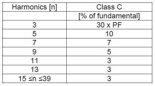
Similar to any other appliance, LED lamps also must comply with several directives which are applicable to the product. The IEC 61000-3-2 standard assesses and sets the limit for equipment that draws input current ≤16A per phase [17-18]. Harmonic emission limits for lamps are subdivided based on their active power up to 25W and above in class C. Lamps having an active input power less than or equal to 25W must satisfy at least one out of the two following criterions. One of the criteria is that the third harmonic current should not exceed 86% of the fundamental and the fifth harmonic current should not exceed 61%. That gives the value of the current THD approximately 105%. The recommended voltage distortion limit for class C equipment is 3% and 5% for individual harmonics and total harmonic distortion (THDV) respectively.
The other criterion is given as a Table 1 for each harmonic order.
Table 1. IEC 61000-3-2 limits for class C equipment (P ≤ 25W)
.
Table 2. Technical data for tested LED lamps
.
Methodology
To analyze the characteristics of the LED lamps with dimming function, 5 samples of with different power ratings from various manufacturers as shown in Table 2 were tested. The lamps have build in ballast which is powered using E-27, E-14 or GU-10 type sockets, commonly available in retail stores. All the tested lamps are designed to operate at 220-240 V and have power consumptions rating of 3 W to 10 W.
Fig.2. Experimental setup
To obtain accurate data concerning the exact current harmonic content of LED bulbs, an experimental setup as shown in Fig. 2 is assembled. It consists of four components namely, Fluke 434 power quality analyzer, Fluke i30s current clamp, LED bulb(s) under test, and a personal computer to analyze the signals. Each lamp is kept switched on for 10 minutes before the measurements are taken for stabilization. Each lamp is tested for four times to eliminate any error during different period of the day. Furthermore, for comparisons purposes, a sample of dimmable CFLs indicated in Table 2 are also tested using the same procedure. The captured current waveforms were analyzed by using Fluke 434 power quality analyser and MATLAB software where the current waveforms of the lamps were transformed using the Fourier Theorem. It provide frequency spectrum of the lamp currents represented by the fundamental sinusoidal component and a series of higher order harmonic components at frequencies that are integer multiples of the fundamental frequency as in (1).
.
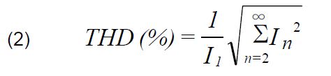
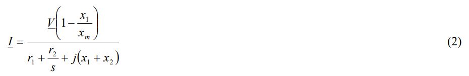
Where I(t) is the input current, In is the harmonic current component of order n. Io is the average current. Furthermore, the square roots of the sum of the amplitudes of the harmonic as in (2) are used to represent the total harmonic distortion (THD).
.
Where I1 is the rms (Route mean square) value of fundamental current and In is the harmonic current component of order n.
Experimental analysis
In this section, measurements of various dimmable LED lamp test were assessed to investigate the harmonic generation when the brightness of the lamps are varied using a Triac dimmer controller commonly used in indo lighting controls. For this findings from the tested lamps at dimming and non dimming mode are analyzed and discussed first. Then a performance comparison of different dimmable LED lamps from various manufactures is conducted. Furthermore, a comparison of dimmable LED and CFL lamps carried out.
General findings from dimmable LED lamps
In order to understand the harmonic patterns of dimmable LED lamps, we consider an Osram 10 W dimmable bulb. The current and voltage wave shape is shown in Fig. 3(a) when it is operated at 0° firing angle of the Triac dimmer representing full brightness of the lamp. From the figure it can be noted that the current waveform is not sinusoidal even at full brightness where the dimmer is not yet activated. It means that this bulb creates and inject harmonic into the power system. However, it is clear from Fig. 3(a), that the voltage wave shape is pure sinusoidal. Therefore only current is distorted. To further investigate, the corresponding harmonic spectrum at 0° firing angle or at non dimming mode Fig. 3(b) plotted. It is noticed that the magnitude of harmonic current decreases with increased harmonic order.
Fig.3. Test results of Osram 10 W dimmable LED lamps at full brightness: (a) Lamp current and voltage waveforms (b) Individual harmonic spectrum
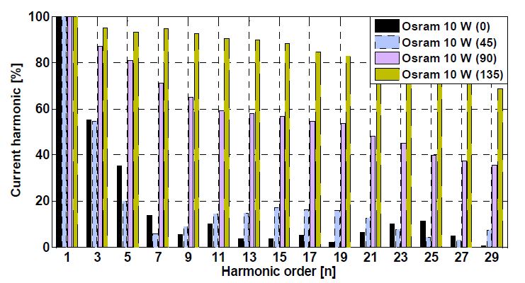
In order to observe the effect of reducing brightness on current harmonics, the dimming angle is increased from 0° to 45°, 90° and 135° respectively. As shown in Fig. 4, it is found that increasing the firing angle of the dimmer, the current drawn by the lamp is more chopped and deviates further from sinusoidal pattern although the magnitude of the current decreases. As a result, harmonic level is increased as depicted in Fig. 5. As seen in Fig. 5, this lamp creates a THDI value of 65%-70% at 0° firing angle (full brightness) whereas it becomes 76%-80% and 230%-235% at 45°and 90° respectively. This increase in THDI may be due to dimming control switch which contribute some additional harmonics.
Findings from Same Wattage LED Lamps
These tests aim to identify the harmonic levels from same wattage lamps introduced by different manufacturers. For this purpose 3 Watt bulbs were investigated. Fig. 6 depicts the wave forms obtained from 3 Watt LED lamps from Philips and Aira brand with 0° delay angles.
From Fig. 6, it is clear that the current wave shape is totally different from Osram 10 Watt bulb because different manufacturers used different type of ballast circuit inside the bulb. The harmonic patterns at various dimming levels of these lamps are shown in Tables 3 and Table 4. For the case of Phillips 3 Watt lamp, it is observed that there is a very large variation of harmonic between 0° and 135°. These harmonic levels are not acceptable for IEC 61000-3-2 standard.
Fig.4. Tested current waveform of Osram 10 W at different dimming mode
Fig.5. Harmonic spectrum of Osram 10 W at different dimming mode
Fig.6. Current and voltage waveform of Philips 3 Watt and Aira 3 Watt lamps at 0° dimming angle
Table 3. Harmonic Content of Philips 3 W with Several Dimming Mode
.
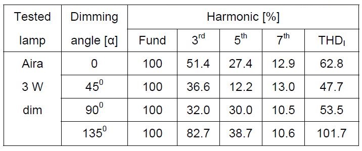
However in the case of Aira brand 3 Watt dimmable lamp, it shows a different characteristic in which harmonic level decrease with decreasing brightness as shown in Table 4. This may be due to the rectangular shape characteristics of the current wave it maintain during the operation. From Fig. 6 it is also clear that the current peaks observed for the case of Aira lamp is much lower than that required by Philips lamp. These high peaks introduce more harmonics into the system. Fig. 7 ill starred current characteristic and harmonic spectrum of those same lamps as discussed in fig. 6 but 45° delay angles.
Table 4. Harmonic Content of Aira 3 W with Several Dimming Mode
.
Fig.7. Comparison of (a) Current waveform, (b) Individual harmonic spectrum of Philips 3 W and Aira 3 Watt lamp at 45° dimming angle
Findings from Same wattage dimmable and non dimmable LED Lamps
The third test investigates the effect of harmonic characteristics of dimmable LED lamps with conventional LED bulbs having same power ratings. For this purpose, 10 Watt normal LED lamp and 10 Watt dimmable LED lamp from Osram as mentioned in Table 2 is compared. Fig. 8 shows the current waveforms along with their harmonic levels for these two lamps at full brightness. From the figure it can be reviled that the distortion level of dimmable LEDs is lower than normal LED lamp at full brightness. However, in case of dimmable bulb, the distortion levels increases rapidly with reduction of brightness. As a result, dimmable lamp at lower brightness is more problematic than conventional LED bulbs.
Fig.8. Test results of Osram 10 W conventional LED lamp with Osram 10 W dimmable LED lamps at full brightness: (a) Lamp current and voltage waveforms (b) Individual harmonic spectrum
Comparison with Dimmable CFLs
Since CFLs are the most commonly used energy efficient lamps today, it is important to compare the performance of new dimmable LED lamps with dimmable CFLs in terms of harmonic generation. For this purpose, Osram brand 20 Watt LED dimmable lamps are compared with 20 Watt dimmable CFLs from same manufacturer. Currently, there is no 20 Watt dimmable LED bulb available in the market so two 10 Watt bulbs of same model is used in parallel for this purpose. This 20 Watt combination gives the same characteristics of 10 Watt LED bulbs. In fact, 20 Watt combination gives a little less harmonic than 10 Watt LED bulb alone.
Fig.9. Current waveform of 10 cycles at 0° dimming angle (a) Osram 20 W CFLs (b) Osram 20 W LED Lamps
Table 5. Harmonic Content of Osram 20 W (Leds and Cfls) Lamps with Several Dimming Mode
.
Fig. 9 depicts the experimental result of current characteristic for Osram 20 Watt dimmable LED and Osram 20 Watt dimmable CFL lamps for 10 cycles at 0° delay angle. From the figure it is clear that the current wave shapes are totally different due to different ballast circuit and the current peak of CFL is almost double to that of LED lamp. A side from current peaks, it is understood from Table 5 that CFL lamp performs better at low brightness but at full brightness LED creates less harmonic.
Conclusion
This paper has presented several experimental results on harmonic generation from dimmable LED lamps that are currently being used for domestic and commercial lighting. In the experiments various types of dimmable LED lamps from different manufactures were tested to evaluate their harmonic performance in terms of power rating, brand, type of ballast used. Furthermore a comparison of harmonic contents of LED lamps and CFLs were also made at dimming mode. Also a comparison of dimmable LED lamps with normal LED lamps in term of harmonic was discussed. Experimental results show that both types of LEDs produce harmonics and increase the value of current total harmonic distortion (THDI) due to the use of power electronic converter as a ballast to drive LED arrays in the bulbs. The value of THDI ranges between 47 % and 360 % for dimmable LEDs bulbs. Moreover, normal LED lamps generate lower harmonic than dimmable ones. Dimmable CFLs also shows similar characteristic like LED counterparts. It is also noted that harmonic characteristics of LED lamps and CFLs of equivalent wattage either at dimmable or non dimmable mode from same vendor depend on the type of ballast used. It is also noted that different manufactures of LED lamps use diverse ballast technologies. Currently there is no standard for dimmable lamps and it is recommended that an individual standard should employ for dimmable operation.
Acknowledgment
This work was carried out with the financial support from the Ministry of Higher Education of Malaysia (MOHE) under the research grant UKM-KK-02-FRGS0193-2010.
REFERENCES
[1] Pinto R.A., Cosetin M.R., Marchesan T.B., Silva M.F.D., Denardin G.W., Fraytag J., Campos A., Prado R.N.D., Design procedure for a compact lamp using high-intensity LEDs, 35th Annual Conference of IEEE Industrial Electronics, (2009), 3506-3511 [2] Leslie R., Raghavan R., Howlett O., Eaton C., The potential of simplified concepts for daylight harvesting, Lighting Research and Technology, 37 (2005), No. 1, 21-38 [3] Rand D., Lehman B., Shteynberg A., Issues, models and solutions for triac modulated phase dimming of LED lamps, IEEE Power Electronics Specialists Conference, (2007), 1398- 1404 [4] Huang H.M., Twu S.H., Cheng S.J., Chiu H.J., A single-stage SEPIC PFC converter for multiple lighting LED lamps, 4th IEEE International Symposium on Electronic Design, Test and Applications, (2008), 15-19 [5] Hu Y., Jovanovic M.M., LED driver with self-adaptive drive voltage, IEEE Trans. Power Electron, 23 (2008), No. 6, 3116-3125 [6] Chiu H.J., Lo Y.K., Chen J.T., Cheng S,J,, Lin C,Y,, Mou S.C., A high-efficiency dimmable LED driver for low-power lighting applications, IEEE Trans. Industrial Electronics, 57 (2010), No.2, 735-743 [7] Xu L., Zeng H., Zhang J., Qian Z., A primary side controlled WLED driver compatible with triac dimmer, 26th Annual IEEE Applied Power Electronics Conference and Exposition, (2011), 699-704 [8] Xu X., Wu X., High dimming ratio LED driver with fast transient boost converter, IEEE Power Electronics Specialists Conference, (2008), 4192-4195 [9] Garcia J., Calleja A.J., Corominas E.L., Gacio D., Campa L., Díaz R.E., Integrated off-line ballast for high brightness LEDs with dimming capability, Journal of Circuits and Systems, 2 (2011), No. 4, 338-351 [10] Borekci S., Dimming electronic ballasts without striations, IEEE Trans. Industrial Electronics, 56 (2009), No. 7, 2464-2468 [11] Cuk V., Cobben J.F.G., Kling W.L., Timens R.B., An analysis of diversity factors applied to harmonic emission limits for energy saving lamps, 14th Intel Conference on Harmonics and Quality of Power, (2010), 1-6 [12] Watson N.R., Scott T.L., Hirsch S.J.J., Implications for distribution networks of high penetration of compact fluorescent lamps, IEEE Trans. Power Delivery, 24 (2009), No. 3, 1521- 1528 [13] Mohamed K., Shareef H., Mohamed A., Analysis of harmonic emission from dimmable compact fluorescent lamps, International Conference on Electrical Engineering and Informatics, (2011), 1-5 [14] Qu X., Wong S.C., Tse C.K., Resonance-assisted buck converter for offline driving of power LED replacement lamps, IEEE Trans. Power Electronics, 26 (2011) No. 2, 532-540 [15] Zhou K., Zhang J.G., Yuvarajan S.A., Weng D.F., Quasi-active power factor correction circuit for HB LED driver, IEEE Trans. Power Electronics, 23 (2008) No. 3, 1410-1415 [16] Shareef H., Mohamed A., Marzuki N., Analysis of ride through capability of low-wattage fluorescent lamps during voltage sags, International Review of Electrical Engineering, 4 (2009), No. 5, 1093-1101. [17] IEEE Std 519-1992, Recommended Practices and Requirements for Harmonic Control in Electrical Power Systems, (The Institute of Electrical and Electronics Engineers, 1993) [18] IEC Std 61000-3-2, Limits for Harmonic Current Emissions (Equipment Input Current ≤ 16A Per Phase), (Ed. 3.2, 2009)
Authors: Sohel Uddin is a Masters student at the Department of Electrical, Electronic and Systems Engineering, Universiti Kebangsaan Malaysia (UKM), E-mail: sohel_091@yahoo.com. Dr. Hussain Shareef is a senior lecturer of Department of Electrical, Electronic and Systems Engineering, Universiti Kebangsaan Malaysia (UKM), E-mail: shareef@eng.ukm.my. Prof. Dr. Azah Mohamed is a professor of Department of Electrical, Electronic and Systems Engineering, Universiti Kebangsaan Malaysia (UKM), E-mail: azah@eng.ukm.my. Dr. M A Hannan is an Associate professor of Department of Electrical, Electronic and Systems Engineering, Universiti Kebangsaan Malaysia (UKM), E-mail: hannan@eng.ukm.m
Source & Publisher Item Identifier: PRZEGLĄD ELEKTROTECHNICZNY, ISSN 0033-2097, R. 89 NR 4/2013
Published by Electrotek Concepts, Inc., PQSoft Case Study: Evaluation of Capacitor Bank Switch Restrikes, Document ID: PQS0606, Date: April 1, 2006.
Abstract: The analysis of high voltage capacitor switching consists primarily of measurements and computer simulations. There are a number of important transient related concerns when transmission and distribution voltage level capacitor banks are applied, including insulation withstand level, switchgear capabilities, energy duties of protective devices, and system harmonic considerations. The considerations should also be extended to include distribution systems and sensitive customer equipment. This case study presents methods for determining transient overvoltage and arrester duties and during capacitor switch restrike events and sample simulation and field measurements of restrike waveforms.
CAPACITOR BANK RESTRIKE EVENTS
A capacitor switching device de-energizes a capacitor bank at a current zero (refer to Figure 1). Since the current is capacitive, the voltage at the time of current interruption is at a system peak. Successful interruption depends on whether the switch can develop sufficient dielectric strength to withstand the rate-of-rise and the peak recovery voltage. For a grounded-wye capacitor bank, two times (2 per-unit) the system voltage will appear across the switch contracts one-half cycle after interruption. If the switch cannot withstand this recovery voltage, the switch will restrike.
Determining Transient Overvoltages and Arrester Duties
The energy duty requirements for arresters at capacitor bank locations depend on the size of the capacitor and on existing arresters located at the substation. In general, the most severe duty for an arrester near a capacitor bank occurs during a switch restrike. This is due to the trapped charge on the capacitor at the instant the restrike occurs, and results in a greater magnitude of the voltage oscillation.
It is also important to consider the coordination of MOV arresters (at the capacitor location) with any conventional gapped type arresters in the substation. It is important that the protective level of the MOV arresters be low enough to prevent operation of the gapped arresters. This is often difficult to achieve. If coordination is not possible, there are three options for arrester protection at the substation involved:
Replace all of the gapped type arresters in the substation with MOV arresters. The arresters will share the energy duty in the event of a restrike and there should be no danger of arrester failure.
Add one set of MOV arresters. This will greatly decrease the probability that a conventional arrester will fail during a capacitor restrike event because the MOV arrester will reduce the chance of a conventional arrester sparkover. The minimum size MOV should be used for best coordination with existing arresters.
Use only conventional gapped type arresters at the substation. This option relies on the integrity of the capacitor switch to prevent a restrike event. If a restrike would occur, it is unlikely the conventional arresters would be able to withstand the associated energy duty.
The arrester energy during a restrike depends on the following parameters:
− Capacitor configuration (grounded vs. ungrounded) − Capacitor size − Existence of other parallel capacitors − Source strength − Number of lines leaving substation − Nearby capacitor banks − Arrester protective level
Arrester applications at large shunt capacitor banks need to be evaluated carefully due to the high-energy duties that can occur in the event of a restrike in the capacitor switch. The energy levels will depend on whether the capacitor bank is grounded or ungrounded.
Figure 1 – Illustration of Capacitor Bank Restrike Event
During normal grounded-wye capacitor bank de-energization, the capacitor current is interrupted at the peak system voltage thus leaving a 1.0 per-unit trapped charge on the capacitor. This trapped charge results in an offset in the transient recovery voltage (TRV) that reaches a magnitude of 2.0 per unit one-half cycle after opening. Significant transient voltages can occur if the switch restrikes during clearing. The worst restrike transient occurs when twice the normal system peak voltage appears across the switch contacts. Theoretically, in this case, the magnitude of the transient voltage approaches 3.0 per unit.
Ungrounded-wye capacitor banks may expose the capacitor switch to recovery voltages greater than 2.0 per unit. Recovery voltages may reach 2.5 per unit on the first phase to open when the other phases open at the next current zero. If two of the phases delay opening, the recovery voltage may reach 3.0 per unit on the first phase to open. Finally, if one of the other phases delays, the transient recovery voltage would be 4.1 per unit. If a restrike occurs on the first phase to open at 2.5 per unit, a recovery voltage of 6.4 per unit can occur on one of the other two phases because of the voltage that builds up across the neutral capacitance. The high recovery voltage on another phase can cause a second restrike, resulting in a two-phase restrike.
The transient voltages on a capacitor bank and the recovery voltages across the switch can be reduced by installing arresters on the capacitor side of the switching device. If the switch is rated for the recovery voltages involved, then the arresters can be located on either the capacitor side or source side of the switch.
To evaluate arrester energy duty, simple expressions can be derived for grounded and ungrounded capacitor banks in terms of capacitor size, source inductance, peak system voltage, and arrester protective levels. The equations for evaluating the energy duty are given in
Table 1 – Arrester Duty during a Capacitor Restrike
.
Assuming a given capacitor bank rating, the arrester energy duty (in joules) versus the arrester protective level can be determined. Figure 2 and Figure 3 illustrate the arrester duty for Metal-Oxide Varistors (MOV). Silicon-Carbide (SiC) arresters generally have more severe energy duties because of the partial capacitor discharge that occurs when the arrester sparks over.
Figure 2 – Theoretical Arrester Duty during a Capacitor Switch Restrike (per-unit of normal peak line-to-neutral voltage)
Figure 3 – Theoretical Arrester Duty, Arrester Capability, and Simulation Results (per-unit of normal peak line-to-neutral voltage)
While the placement of an MOV arrester on the capacitor side of the breaker is not required, it is generally recommended. This location provides overvoltage protection for the bank itself, as well as limiting the recovery voltage seen by the breaker. Another benefit of the arrester is that its presence should help to minimize the possibility of multiple restrike events. Previous experience has indicated that if a breaker experiences multiple restrikes during clearing, equipment failure will more than likely occur.
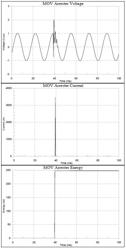
Figure 4 illustrates an example of a computer simulation showing arrester (MOV) voltage, arrester current, and arrester energy duty during a capacitor switch restrike.
Figure 4 – Simulated Arrester Voltage, Current, and Energy during Switch Restrike
Sample Simulations and Field Measurements of Restike Events
Figure 5 shows the bus voltage (in per-unit) during a multiple restrike event on a 50 MVAr, 230kV transmission capacitor bank. The capacitor bank is protected with an 180kV MOV arrester.
Figure 6 shows the bus voltage during de-energization and switch restrike of a 161kV transmission capacitor bank. The worst-case transient voltage was approximately 2.02 per-unit (202%).
Figure 6 – 161kV Capacitor Switch Restrike
Figure 7 shows the bus voltage during a multiple restrike event on a 34.5kV capacitor bank. The worst-case transient voltage was approximately 1.55 per-unit (155%).
Figure 7 – 34.5kV Multiple Capacitor Switch Restrike Voltage
Figure 8 shows the transformer secondary current during a multiple restrike event on a 34.5kV capacitor bank.
Figure 8 – 34.5kV Transformer Current during Multiple Capacitor Switch Restrike
SUMMARY
Arrester energy during a capacitor switch restrike event is dependent on the capacitor configuration, ratings, source strength (including nearby capacitors and number of transmission lines), and arrester protective level (e.g., maximum switching surge protective level – MSSPL).
A properly sized MOV arrester, placed between a capacitor switch and a capacitor bank, will provide overvoltage protection for a single restrike event. In addition, the arrester will protect the bank from excessive overvoltages, as well as reduce the likelihood of multiple restrike events that can result in equipment failure.
REFERENCES
G. Hensley, T. Singh, M. Samotyj, M. McGranaghan, and T. Grebe, Impact of Utility Switched Capacitors on Customer Systems Part II – Adjustable Speed Drive Concerns, IEEE Transactions PWRD, pp. 1623-1628, October, 1991.
G. Hensley, T. Singh, M. Samotyj, M. McGranaghan, and R. Zavadil, Impact of Utility Switched Capacitors on Customer Systems – Magnification at Low Voltage Capacitors, IEEE Transactions PWRD, pp. 862-868, April, 1992.
T.E. Grebe, Application of Distribution System Capacitor Banks and Their Impact on Power Quality, 1995 Rural Electric Power Conference, Nashville, Tennessee, April 30-May 2, 1995.
M. McGranaghan, W.E. Reid, S. Law, and D. Gresham, Overvoltage Protection of Shunt Capacitor Banks Using MOV Arresters, IEEE Transactions PAS, Vol. 104, No. 8, pp. 2326-2336, August, 1984.
S. Mikhail and M. McGranaghan, Evaluation of Switching Concerns Associated with 345 kV Shunt Capacitor Applications, IEEE Transactions PAS, Vol. 106, No. 4, pp. 221-230, April, 1986.
T.E. Grebe, Technologies for Transient Voltage Control During Switching of Transmission and Distribution Capacitor Banks, 1995 International Conference on Power Systems Transients, September 3-7, 1995, Lisbon, Portugal.
Electrotek Concepts, Inc., An Assessment of Distribution System Power Quality – Volume 2: Statistical Summary Report, Final Report, EPRI TR-106294-V2, EPRI RP 3098-01, May 1996.
Electrotek Concepts, Inc., Evaluation of Distribution Capacitor Switching Concerns, Final Report, EPRI TR-107332, October 1997.
RELATED STANDARDS IEEE Std. 1036
GLOSSARY AND ACRONYMS MOV: Metal Oxide Varistor Arrester MSSPL: Maximum Switching Surge Protective Level SiC: Silicon Carbide Arrester TRV: Transient Recovery Voltage
Published by Electrotek Concepts, Inc., PQSoft Case Study: Customer Adjustable-Speed Drive Motor Failure Evaluation, Document ID: PQS1010, Date: October 15, 2010.
Abstract: This case study presents a customer adjustable-speed drive motor winding failure analysis. The study investigated the potential for severe high frequency transient overvoltages at induction motor terminals for an adjustable-speed drive that utilized a pulse-width modulation inverter, along with a significant length of cable between the inverter and motor. Several power conditioning mitigation alternatives including series reactors and motor terminal filters were evaluated using computer simulations.
INTRODUCTION
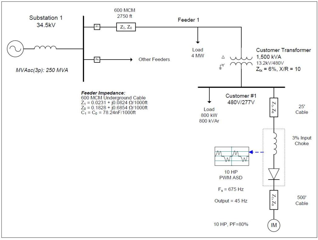
A customer adjustable-speed drive (ASD) motor winding failure case study was completed for the system shown in Figure 1. The case study investigated the potential for severe high frequency transient overvoltages at induction motor terminals for an adjustable-speed drive that utilizes a pulse-width modulation (PWM) inverter, along with a significant length of cable between the inverter and induction motor. Several power conditioning mitigation alternatives, such as series reactors/chokes and motor terminal filters, were evaluated using computer simulations.
The simulations for the case study were completed using the PSCAD program. The accuracy of the simulation model was verified using three-phase and single-line-to-ground fault currents and other steady-state quantities. The circuit consisted of a 34.5 kV utility substation supplying a 1,500 kVA customer step-down transformer, along with a 10 hp PWM adjustable-speed drive with a 500 foot cable segment between the inverter and motor terminals. A high frequency, distributed parameter transmission line model was required to accurately represent the traveling wave (reflections) effects of the motor cable. There was also a standard 3% input choke on the drive, which resulted in a current distortion value of approximately 40.9%. A detailed drawing of the adjustable-speed drive and induction motor configuration is shown in Figure 2.
Figure 1 – Illustration of Oneline Diagram for Customer Motor Failure Evaluation
Figure 2 – Illustration of Adjustable-Speed Drive and Motor Circuit
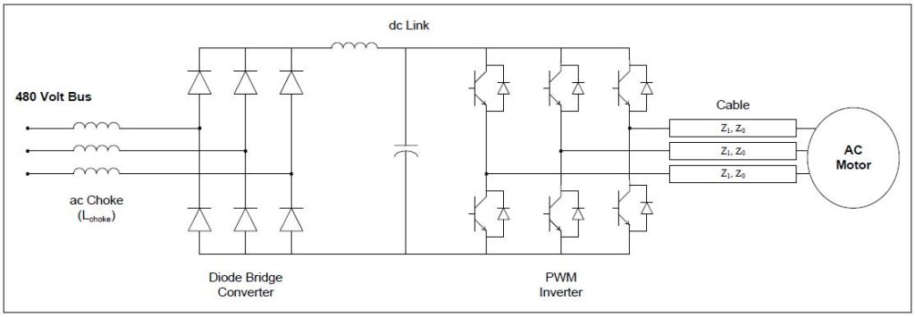
Adjustable-speed drives for most small and medium induction motors utilize voltage source inverters to provide variable frequency ac output. The common drive structure adopted by the industry consists of an uncontrolled diode-bridge rectifier, dc link, and pulse-width modulation voltage source inverter as illustrated in Figure 3. The dc link for this type drive includes a ripple smoothing capacitor. The inverter output waveform is generated by a series of step-like functions. An ideal step-change in the output voltage is prevented by stray parameters of the circuit and commutation of switching devices from one phase to another. Steep-front waveform generation is one of the inherent characteristics of a high switching frequency voltage source inverter.
SIMULATION RESULTS
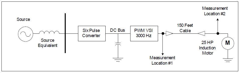
The output voltage of the pulse-width modulation inverter is a potential problem for the induction motor. Both the frequency and magnitude of the output voltage are adjusted by controlling the inverter’s operation. State-of-the-art voltage source inverters are based on insulated gate bipolar transistor technology. With these devices, the inverter operates with a switching frequency ranging from tens of Hz to tens-of-thousands of Hz. Figure 4 shows an example output voltage of a pulse-width modulation drive (measurement location #1 on Figure 3). The switching frequency of the most commonly used pulse-width modulation drives is in the range of 1,000 Hz to 5,000 Hz. The rise times of the pulses can be approximately 10μs to 0.1μs.
The problem occurs on the output of the inverter at the drive terminals. The high switching frequency of the inverter allows sophisticated control schemes to be implemented. One of the advantages of the high switching frequency inverter is the reduction of low order harmonics, which results in a reduction of output filter duty. However, this benefit can only be achieved under certain circuit conditions. Under some conditions, the fast changing voltage resulting from high frequency switching operation of inverter can create severe insulation problems for induction motors.
Machine insulation integrity is influenced by the rate-of-change of voltage as well as the transient overvoltage magnitude. A voltage with a high rate-of-change tends to be distributed along a motor’s windings unevenly. This uneven distribution causes a significant over-stress across ending turns resulting in turn-to-turn insulation failure. In practice, it is common for the drive and the motor to be separated by relatively long lengths of cable. In addition, the characteristic impedance of the induction motor can be ten to one hundred times that of the characteristic impedance of the cable connecting the drive to the induction motor.
Figure 3 – Oneline Diagram Showing Power System and Inverter Circuit
Figure 4 – Measured Example Line-to-Line Output Inverter Voltage
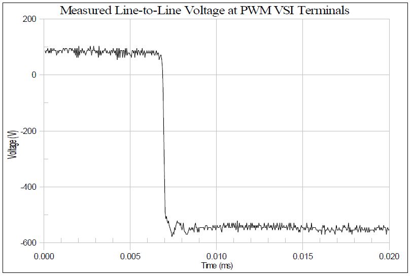
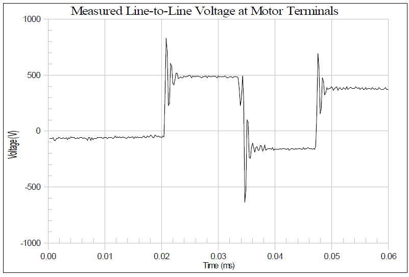
Figure 5 shows a transition in one of the pulses at the inverter (measurement location #1). Notice that when the voltage changes from zero to its full negative value, there is no significant over-shoot or overvoltage. At the motor terminals, however, the transition of one of the pulses at the motor terminals shows an overvoltage of approximately 1.7 per-unit, as shown in Figure 6 (measurement location #2). The overvoltage and the resulting ringing occur at both the front and rear of each pulse. Depending on the operation pattern of the adjustable-speed drive, similar transients may occur 20 to 100 times per 60 Hz cycle.
The most harmful effect of the inverter output occurs when the connection cable is relatively long with respect to the wave front of an incidental voltage wave and when the ratio of characteristic impedance of the machine and the cable is high. In the worst case, an inverter output voltage pulse magnitude can be doubled at the induction motor terminals. If a voltage wave travels at a velocity of 250 feet per microsecond, an incident voltage wave with a front time of 0.3μs is sufficient to create a voltage doubling at the open end of 75 feet of cable. Under this condition, motor windings experience a near 2.0 per-unit over voltage, if the maximum voltage seen at the inverter output terminal is 1.0 per-unit.
Figure 5 – Measured Example Phase-to-Phase Voltage at Inverter Terminals
Figure 6 – Measured Example Phase-to-Phase Voltage at Motor Terminals
The reflection of an incident traveling voltage wave at the motor connection termination is determined by surge impedance ratio at the junction point. The characteristic impedance of a small motor is usually higher than the low surge impedance of the cable. Therefore, when compared with the low surge impedance of cable, the motor connection may look like an open circuit.
The initial simulation (Case 4a) involved the basecase condition with no mitigation added to the adjustable-speed drive or induction motor.
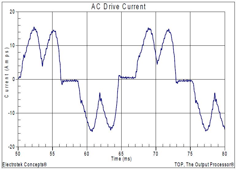
Figure 7 shows the simulated current waveform (single phase shown) for the 10 hp adjustable-speed drive operating at an 80% power factor and with a 3% ac choke. The current has a fundamental frequency value of 8.5 A, an rms value of 9.1 A, and a THD value of 40.9%.
Figure 7 – Simulated AC Drive Current Waveform
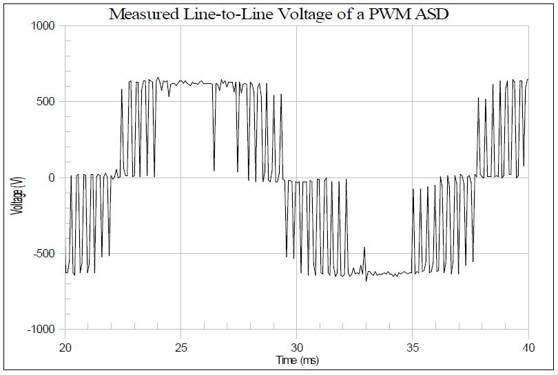
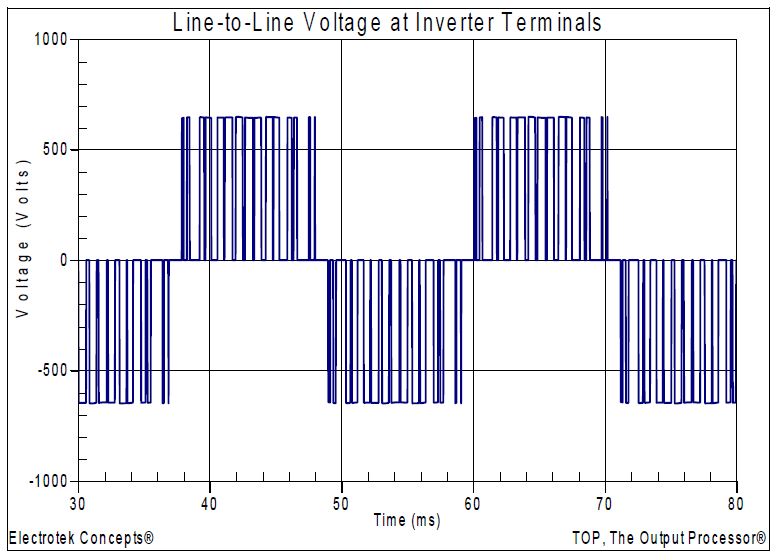
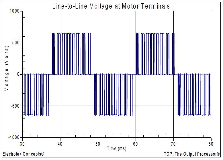
Figure 8 shows the simulated line-to-line voltage at the inverter terminals for the basecase conditions. The dc voltage for the drive was approximately 650 V. The inverter switching frequency (Fs) for the case was 675 Hz and the motor frequency was 45 Hz.
Figure 8 – Simulated Line-to-Line Inverter Voltage Waveform
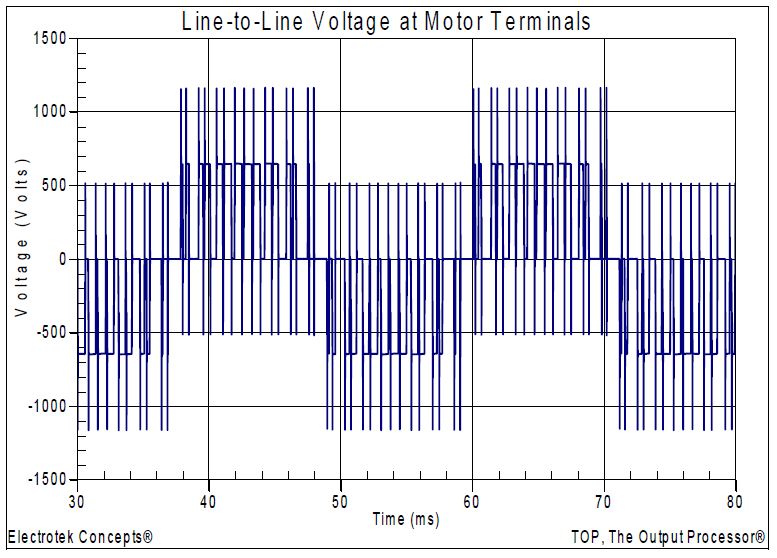
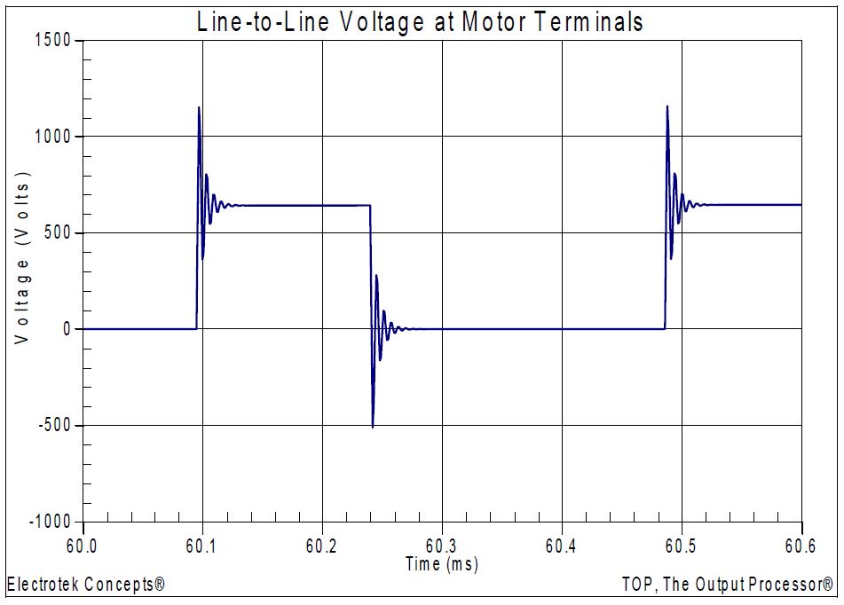
Figure 9 shows the simulated line-to-line voltage at the motor terminals for the case with no mitigation added. Figure 10 shows an expanded view of the waveform highlighting several of the ringing transients. The peak simulated transient voltage was 1,153V, which was approximately 1.77 per-unit (similar to the measured waveform previously shown in Figure 6).
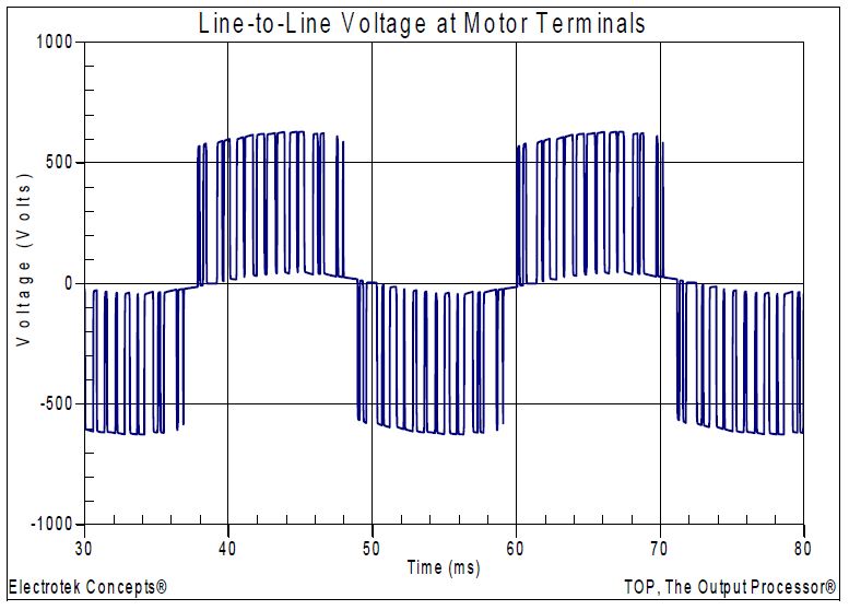
Figure 9 – Simulated Line-to-Line Motor Voltage Waveform
Figure 10 – Expanded View of Line-to-Line Motor Voltage Waveform
The second simulation case (Case 4b) evaluated the power conditioning alternative of adding a series choke between the inverter and the induction motor. Inductive chokes (a.k.a., reactors) are similar to isolation transformers, except that they do not define a separately derived system. Inductive chokes provide additional impedance in the circuit in much the same manner that an isolation transformer does, but at a much-reduced cost.
Chokes are often applied to the front-end of adjustable-speed drives to protect the drives from nuisance tripping caused by utility capacitor bank switching and other normal power system switching operations. Some drive manufacturers now produce drives with chokes as part of their standard design. Chokes also help prevent voltage notching, caused by power electronic switching, from disturbing other sensitive customer equipment. They can limit notching to the drive side of the inductive choke.
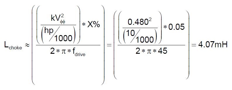
Figure 11 shows the simulated line-to-line voltage at the induction motor terminals for the case with a 5% choke added between the inverter and motor terminals. Generally, a choke is specified in %X and hp. The inductance of the simulated choke rating was approximated using the following expression:
.
where: fdrive = inverter output fundamental frequency (Hz) X = inductive reactance of choke (%) kVϕϕ = system rms phase-to-phase voltage (kV) hp = horsepower rating of the motor (hp)
The resulting transient voltages at the motor terminals were significantly reduced with the 5% choke. It should be noted that the fundamental drive frequency voltage was somewhat lower due to the voltage drop across the choke.
The final simulation case (Case 4c) evaluated the power conditioning alternative of adding a motor terminal filter to the induction motor. A motor terminal filter is a type of low-pass filter that passes signals with low frequencies and reject signals with high frequencies. These filters can improve power quality by reducing the effect of the transient energy and by removing noise from the electrical system. Low-pass filters can be used to provide even better protection than inductive reactors for high frequency transients.
A first-order filter consisting of a capacitor in series with a resistor can be designed to have minimal losses and to match the surge impedance of the cable that supplies the motor.
Figure 11 – Simulated Line-to-Line Motor Voltage Waveform with 5% Choke
Figure 12 shows the simulated line-to-line voltage at the induction motor terminals for the case with a shunt motor terminal filter added at the motor terminals. The simulated filter component values were 1μF (capacitor) and 100Ω (resistor). The transient voltages were significantly reduced with the motor terminal filter, as compared with the basecase conditions. It should be noted that there was no fundamental drive frequency voltage drop for this case because the filter was connected in shunt, rather than in series like the previous case.
Figure 12 – Simulated Line-to-Line Motor Voltage Waveform with Motor Terminal Filter
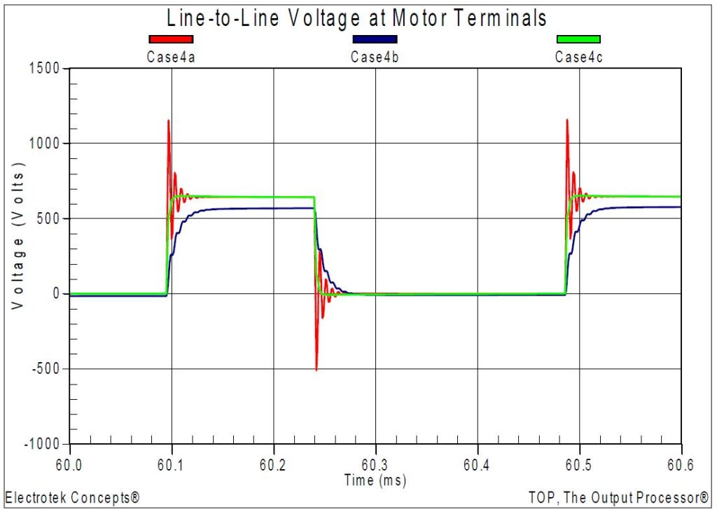
Figure 13 shows an expanded view of the simulated line-to-line voltages at the motor terminals for the three simulated cases. The figure illustrates the reduced transient voltages with the mitigation alternatives and the voltage drop for the 5% series choke case (Case 4b).
Figure 13 – Simulated Line-to-Line Motor Voltage Waveforms
SUMMARY
This case study presented a customer adjustable-speed drive motor winding failure analysis. The study investigated the potential for severe high frequency transient overvoltages at induction motor terminals for an adjustable-speed drive that utilized a pulse-width modulation inverter, along with a significant length of cable between the inverter and motor.
In the past, the inverters for many drives were thyristor based with either forced-commutation or loadcommutation. For current source inverter (CSI) drives based on thyristor or gate turn-off (GTO) devices, the inverter switching frequency was limited to several hundred Hz. This low switching frequency means that these devices have relatively high commutation losses and need a relatively long commutation period. Consequently, induction motors supplied from current source inverter drives have a lower probability of experiencing fast-front transient voltages.
In an effort to improve the efficiency of many industrial processes, standard induction motors have been retrofitted with adjustable speed drives. The drives allow for better speed control, soft starting of motors, and increased efficiency of the overall process operation. Unfortunately, there can also be some power quality-related drawbacks when using these drives.
A number of drive manufacturers are working with motor manufacturers to match drive-duty induction motors to their adjustable-speed drives. The adjustable-speed drive and motor are provided as a complete package. The induction motors are designed to withstand the severe duties imposed on them by the high switching frequencies of the PWM inverters.
This case study investigated one of potential problems with applying new adjustable-speed drives with older induction motors, which is motor winding failure due to transient overvoltages. The power conditioning solutions that were evaluated included series chokes and shunt motor terminal filters. Other potential solutions include changing the cable length, which is generally not practical for the customer; and changing the inverter switching frequency, which may also not be practical and may not significantly reduce the transient overvoltages.
REFERENCES
IEEE Recommended Practice for Monitoring Electric Power Quality,” IEEE Std. 1159-1995, IEEE, October 1995, ISBN: 1-55937-549-3.
IEEE Recommended Practice for Emergency & Standby Power Systems for Industrial & Commercial Applications (IEEE Orange Book, Std. 446-1995), IEEE, ISBN: 1559375981.
IEEE Recommended Practice for Powering and Grounding Electronic Equipment (IEEE Emerald Book, Std. 1100-1999), IEEE, ISBN: 0738116602.
Melhorn, C.J., and Tang, L., “Transient Effects of PWM Drives on Induction Motors,” IEEE Transactions on Industry Applications, Volume 33, Issue 4, pp. 1065-1072, Jul/Aug 1997.
R.C. Dugan, M.F. McGranaghan, S. Santoso, H.W. Beaty, “Electrical Power Systems Quality,” McGraw-Hill Companies, Inc., November 2002, ISBN 0-07-138622-X.
Published by Electrotek Concepts, Inc., PQSoft Case Study: Study of 345 kV Transient Recovery Voltages, Document ID: PQS0602, Date: January 1, 2006.
Abstract: Transient recovery voltage (TRV) is the voltage across the terminals of a pole of circuit breaker following current zero when interrupting faults. TRV waveshapes can be oscillatory, exponential, cosine-exponential or combinations of these forms. TRVs due to short-line faults (SLFs) are characterized by triangular-shaped waveshapes and a very steep initial rate-of-rise. An engineering study found that for a number of cases, the TRV waveshapes exceeded their related TRV capability limits for the first 10-50 μsec. The results also indicated that clearing SLFs on lines leaving the 345kV substations would result in an initial rate-of-rise of the recovery voltage (RRRV) that exceeds the breaker’s SLF capability. The study evaluated the application of an additional capacitance on the line side of the circuit breakers. This capacitance reduces the initial RRRV to within the related SLF capability. This case study presents a summary of the model development and simulations completed during the 345kV TRV study.
INTRODUCTION
Due to the concern for excessive TRVs during breaker operations, an engineering study was preformed to evaluate the proposed 345kV substation design, as well as the impact on nearby utility equipment. The study evaluated the concerns and possible solutions, such as adding capacitive devices, to protect against the harmful transients that may damage the surrounding equipment and power system.
The analysis of high-frequency TRVs frequently requires the use of sophisticated digital simulation tools. Simulations provide a convenient means to characterize transient events, determine resulting problems, and evaluate possible mitigation alternatives. Occasionally, they are performed in conjunction with system monitoring for verification of models and identification of important power system problems. The complexity of the models required for the simulations generally depends on the system characteristics and the transient phenomena under investigation.
The transient analysis for the study was performed using the PSCAD program. This program can be used for the analysis of circuit switching operations, capacitor switching, lightning transients, and transients associated with the operation of power electronic equipment.
STUDY METHODOLOGY
The TRV evaluation for various fault conditions was based on the methods provided in IEEE Std. C37.06, IEEE Std. C37.04, and IEEE Std. C37.011. This involved analysis of the most severe conditions, including the clearing of a three-phase ungrounded symmetrical fault at the breaker terminal when the system voltage is at a maximum and SLFs.
The study considered normal cases where the system operates with all breakers and lines in service and various contingencies where only one breaker is available to clear a fault. For both of these conditions, three-phase ungrounded and single-line-to-ground faults were evaluated.
TRV is the voltage across the terminals of a pole of circuit breaker following current zero when interrupting faults. TRV waveshapes can be oscillatory, exponential, cosine-exponential or combinations of these forms. TRVs due to SLFs are characterized by triangular-shaped waveshapes and a very steep initial rate-of-rise. The triangular shape of the recovery voltage arises from positive and negative reflections of the traveling waves that oscillate between the open breaker and the fault. Due to the short distance involved between the fault location and the open breaker, the initial RRRV can be very steep.
According to IEEE Std. 37.011-1994, the most severe oscillatory or exponential recovery voltages tend to occur across the first pole to open of a circuit breaker interrupting a three-phase ungrounded symmetrical fault at its terminal when the system voltage is at a maximum. When the TRV performance meets the withstand criteria when subjected to the fault condition mentioned above, a SLF evaluation is not necessary. This is due to the fact that SLF TRV capability is higher than that of a three-phase ungrounded fault.
MODEL DEVELOPMENT
The model development process included steps for data collection, data approximation, data simplification and model verification.
The TRV system model was based on short-circuit data that consisted of positive and zero sequence impedance data in the ASPEN Oneliner format. The study area included the substation and the adjacent system (see Figure 1). The boundary of the study area was represented with equivalent sources and transfer impedances such that the electrical representation of the study area (at 60 Hz) was nearly identical to the original representation.
Figure 1 – System Model for the 345kV TRV Study
In the study, all transmission lines were represented with a frequency dependent line model to account for traveling wave phenomena. Generating units were represented with ideal sources behind sub-transient impedances. The accuracy of the transient model was verified by comparing three-phase and single-line-to-ground fault currents at all buses. A subset of the fault cases is summarized in Table 1.
Table 1 – Steady-State Fault Simulations Completed for Model Verification
.
The model represented a reduction of the entire system to determine the system equivalents and corresponding fault levels. It should be noted that the corresponding PSCAD model did not include mutual coupling between transmission lines. In addition, typical X/R ratio values were used where the short-circuit model did not include resistance (e.g., lines, transformers, etc.), and relatively large transfer impedances were ignored. Considering these factors, accuracy within 3% was considered acceptable for the 60 Hz short-circuit model verification.
Circuit Breaker Data
In evaluating the TRV withstand capability for the 345kV breakers, the following references were used:
ANSI C37.06-2000 Tables 3 and 6 (Note 6 for Table 3)
IEEE C37.04-1999, Section 5.9, Table 2 and Figure 5
The new 345kV breakers have the following ratings:
Rated Maximum Voltage: 362 kV Rated Continuous Current: 3000 A Rated Short-Circuit Current: 63 kA Rated Interrupting Time: 2 Cycles Rated Transient Inrush Current: 25 kA Rated Transient Inrush Current Frequency: 4250 Hz
TRV-related data is shown in Table 2 and Table 3.
Table 2 – Rated TRV Capability of 362kV, 3000 A, 63kA Breaker
.
Table 3 – Multipliers for Various Interrupting Levels for Terminal Faults
.
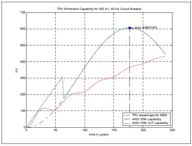
The waveshape of the exponential component E1 for terminal faults below 30% of the breaker rating is 1-cosine. Based on Table 2 and Table 3 and the discussion in Section 5.9 of IEEE Std. C37.04-1999, the TRV limit envelopes were derived and graphically represented using a MATLAB program. Figure 2 shows the TRV envelopes (or withstand capabilities) for several fault levels. Capability envelopes when interrupting fault currents below 30% of its rated short-circuit current have a waveshape of 1-cosine, while for fault currents above 30% of breaker rating, the waveshape has an exponential-cosine form.
Figure 2 – TRV Withstand Capability for a 362kV, 3000 A, 63kA Breaker
Capacitance Values for Substation Equipment
Equivalent values of capacitance for substation equipment were the lumped values at the breaker terminals. Since the capacitance values for the 345kV equipment at the studied substations were not supplied by the utility, it was agreed that typical capacitance ranges based on Annex B of IEEE Std. C37.011-1994 would be used. Three equivalent capacitance values (minimum, maximum, and average) were determined. Table 4 shows an example of the collection of typical capacitance values for each bus section in the model.
Table 4 – Typical Capacitance Values Based on Annex B of IEEE Std. C37.011-1994
.
This process was repeated for all of the 345kV substation equipment in the system model. The minimum values of equivalent capacitance were used throughout the simulation process for both normal and contingency cases.
SIMULATION RESULTS
The TRV evaluation was conducted for the most severe operating conditions, including both three-phase ungrounded faults at the breaker terminal and SLFs. The study considered both normal cases where the system operates with all breakers and lines in service and contingency cases where the only one breaker is available to clear the fault.
Three-Phase Ungrounded Terminal Faults
The simulation results for the three-phase ungrounded fault clearing cases were summarized in tables similar to Table 5. The table shows the respective case identifier, the breaker number, the peak current that the breaker interrupted, this peak current as a percentage of the rated value (63kA), the peak TRV in kV, and a note to report whether the TRV was within the breaker’s capability envelope. A “YES*” note signifies that the TRV waveshape slightly exceeded the TRV capability for the first 10-50 μsec, but it met the TRV SLF capability. A “NO” note signifies that the TRV waveshape did not meet the TRV capability limit.
Table 5 – TRV Evaluation of Three-Phase Terminal Faults
.
Figure 3 and Figure 4 show several examples of the simulation results for the three-phase ungrounded fault clearing cases summarized in Table 5. Figure 3 shows the recovery voltage for breaker 4560 for Case A1 and Figure 4 shows the recovery voltage for breaker 4592 for Case A3. Each graph of TRV includes an overlay of the withstand capability.
Figure 3 – TRV Withstand Capability for Breaker 4560 for a Three-Phase Ungrounded Fault
Figure 4 – TRV Withstand Capability for Breaker 4592 for a Three-Phase Ungrounded Fault
Short-Line Faults
The simulation results for the SLF cases were recorded and compared to their respective TRV withstand and SLF capabilities. Figure 5 shows an example of the simulation results for a SLF clearing case. When compared to their respective terminal fault case, the magnitude of the peak fault current interrupted was lower due to the additional line impedance between the fault location and the breaker terminals. However, the RRRV was higher due to the traveling waves that oscillate between the fault location and breaker terminals.
Figure 5 – TRV Withstand Capability for Breaker 4564 for a Three-Phase Ungrounded SLF
As can be seen in Figure 5, the initial TRV for the case with no added capacitance exceeds the related SLF capability. Additional cases were then completed for each faulted transmission line to evaluate the effectives of various capacitance values for reducing the RRRV for each 345kV substation breaker. The case with 15ηF added is shown in Figure 6.
Figure 6 – TRV Withstand Capability for Breaker 4564 with 15nF Added
SUMMARY
The engineering study included an evaluation of the TRV performance for various breaker operations for new 345 kV breakers. A number of observations and conclusions based on the simulation results included:
1.The TRV evaluation for the new 345kV circuit breakers in the substations was conducted for the most severe operating conditions, including clearing both three-phase ungrounded faults at the breaker terminal and SLF.
2.Three capacitance values, representing a range of equivalent capacitances for substation equipment, were determined based on information provided by the utility and from Annex B of IEEE Std. C37.011-1994.
3.The TRV evaluation considered both normal cases where the system operates with all breakers and lines in service and contingency cases where only one breaker is available to clear a fault. Both three-phase ungrounded and single-line-to-ground faults were evaluated for these conditions.
4.For a number of cases, the TRV waveshapes exceeded their related TRV capability limit for the first 10-50 μsec after the breaker had opened. These cases were then compared to their corresponding SLF capability.
5.For a number of normal and contingency cases, the TRV waveshapes exceeded their related capability limit. For these cases, the breaker’s withstand capability was exceeded due to the peak of the recovery voltage, rather than the initial rate-of-rise.
6.With respect to clearing SLF on lines leaving the 345kV substations (2 km from the substation), the simulations indicated that the initial RRRV will exceed the related SLF capability. One method for mitigating this condition is with the application of an additional capacitance on the line side of the breaker. This capacitance reduces the initial RRRV to within the related SLF capability.
7.Simulations were completed to evaluate the application of an additional capacitance on the line side of breakers. These cases used the same capacitance values at each of the line terminals. The additional capacitance of 15ηF/phase generally reduced the initial RRRVs to within the related SLF capability.
REFERENCES
Study of 345kV Transient Recovery Voltages on the Illinois Power System, Sixth International Conference on Power System Transients (IPST), Montreal, Canada, June 19-23, 2005.
IEEE AC High Voltage Circuit Breakers Rated on a Symmetrical Current Basis – Preferred Ratings and Related Required Capabilities, IEEE Standard C37.06, May. 2000.
IEEE Standard Rating Structure for AC High-Voltage Circuit Breakers, IEEE Standard C37.04, June. 1999.
IEEE Application Guide for Transient Recovery Voltage for AC High Voltage Circuit Breakers Rated on a Symmetrical Current Basis, IEEE Standard C37.011, September. 1994.
Published by Electrotek Concepts, Inc., PQSoft Case Study: Common Power Quality Waveform Signatures, Document ID: PQS0901, Date: October 15, 2009.
Abstract: Power quality problems encompass a wide range of disturbances and conditions on utility and customer power systems. They include everything from very fast transients (microseconds) to long duration (hours) outages. Problems also include steady state (e.g., harmonic distortion) and intermittent (e.g., voltage flicker) phenomena. This wide variety of conditions makes the development of standard measurement and analysis procedures very difficult. Therefore, it is beneficial to characterize power quality measurements and their related problems into common categories using standard data formats.
This case study presents a collection of representative waveforms for various power system fault and power quality events, including voltage sags, momentary interruptions, voltage swells, harmonics, capacitor switching transients, transformer energizing transients, and ferroresonance.
INTRODUCTION
The term power quality refers to a wide variety of different parameters that characterize the voltage and current at a given time and at a given point on the power system. It is important to have a clear understanding of these parameters and the variations in them that can cause customer problems. Definitions are required to develop a method of categorizing problems so that conditions at different sites can be compared and analyzed.
This case study refers to power quality variations and disturbances. Disturbances signify onetime, momentary events while power quality variations refer to the full range of conditions that can occur, including variations in steady-state voltage and current characteristics (e.g., harmonic distortion). There are currently no clearly accepted definitions for many categories of power quality variations because different manufacturers of measurement equipment often use non-standard definitions to categorize events. In addition, individual industry standards address only a small segment of the total range of power quality variations. Several important factors that should be considered when using power quality categories include:
− The characteristics of the power quality variation. Important characteristics include the magnitude, frequency content, and duration. Some combination of these characteristics can be used to describe virtually any power quality variation.
− The cause of the power quality variation. The condition could be caused by a switching event, lightning, a system fault, or operation of customer equipment. It is important to consider the possible causes of power quality variations in each category.
− Requirements for measurement. Some types of power quality variations can be characterized with simple voltmeters, ammeters, or strip chart recorders. Other conditions require special-purpose disturbance monitors or harmonic analyzers. The characteristics of the power quality variation in each category determine the requirements for monitoring.
− Methods to improve the power quality. Solutions to power quality problems depend on the type of power quality variation involved. Transient disturbances can often be controlled with surge arresters while momentary interruptions could require an uninterruptible power supply (UPS) system for equipment protection. Harmonic distortion may require special-purpose harmonic filters.
− Existing standards and power quality terminology. Existing terminology has become almost standard in describing many types of power quality variations. This terminology has resulted from the definitions used to describe power quality by popular monitoring equipment manufacturers and from the development of standards for some aspects of power quality. When developing a new set of definitions for power quality variations, the existing terminology should be carefully considered.
POWER QUALITY CATEGORIES
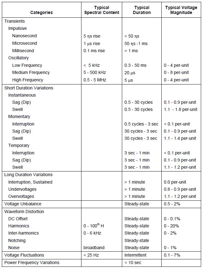
The relative importance of a particular category of power quality phenomena for a specific customer will depend on the type of installed electrical equipment. The type of interaction between customer equipment and the power quality phenomena – equipment damage, equipment/process trip, compromised product quality, etc. – and the frequency at which it occurs or could be expected to occur are also critical factors in the evaluation process once the cause has been identified. The range of power quality phenomena is defined by IEEE Std. 1159-1995: Recommended Practice for Monitoring Electric Power Quality (refer to Table 1) [1].
Approaches for resolving equipment or process problems related to each category of phenomena vary widely. Causes, impacts, and appropriate solutions for this range of electrical phenomena have been analyzed in numerous research and study efforts, resulting in the development of proven solution techniques for many common power quality problems.
These efforts have also contributed to a prioritization of the power quality phenomena categories. From the customer’s point of view, the most important problem categories:
− Have the highest negative impact on productivity − Are difficult to diagnose and characterize − Are more difficult and/or expensive to resolve
Using these criteria, research and case study investigations have identified the following categories of power quality phenomena to be of highest importance to customers:
− Transients, especially utility capacitor bank switching transients − Harmonic distortion, especially resonance conditions − Voltage variations, especially rms voltage sags and interruptions
This does not mean that there are never problems associated with other categories of power quality phenomena. Experience does indicate, however, that the majority of problems (especially from the customer’s perspective) are those listed above.
Table 1 defines power quality variation categories. Some of the categories also include subcategories for more accurate description of particular power quality variations. Three primary attributes are used to differentiate among the different categories and subcategories:
Frequency components
Magnitude
Duration
These attributes are not equally applicable to all the categories of power quality variations. For instance, it is difficult to assign a duration to an oscillatory transient, and it is not useful to assign a spectral content to variations in the fundamental frequency magnitude (e.g., sags, swells, overvoltages, undervoltages, and interruptions). Each category is defined by the most important attributes for that particular power quality condition.
These characteristics and attributes are useful for evaluating measurement equipment requirements, system characteristics affecting the power quality variations, and possible measures to correct power quality problems.
This case study presents a number of representative waveforms for an assortment of power system fault and power quality events, which are grouped by the categories provided in IEEE Std. 1159-1995 and shown in Table 1.
Table 1 – Categories of Power System Electromagnetic Phenomena (source IEEE Std. 1159-1995)
.
POWER QUALITY DATA FORMATS
This case study illustrates a number of representative power quality event waveforms that are stored using the common data interchange formats PQDIF and COMTRADE. PQDIF [2] provides a recommended practice for a file format suitable for exchanging power quality related measurement and simulation data. COMTRADE [3] provides a common format for digital data records of power system fault, test, or simulation events.
PQDIF (IEEE Recommended Practice for the Transfer of Power Quality Data) is an IEEE standard (1159.3-2003) that was developed by the Working Group on Monitoring Electric Power Quality, which is part of the Power Quality Subcommittee of the T&D Committee. It defines a file format suitable for exchanging power quality related measurement and simulation data in a vendor-independent manner. A variety of simulation, measurement and analysis tools for power quality engineers are now available from many vendors. Generally, the data created, measured, and analyzed by these tools are incompatible between vendors. PQDIF provides a set of requirements and attributes for a power quality data interchange format. Key among these is the ability to represent data from a variety of sources (e.g., measured, simulated, or manually created), in the time, frequency, and probability domains.
COMTRADE (IEEE Standard Common Format for Transient Data Exchange for Power Systems) is an IEEE standard (C37.111-1999) first published by the Power System Relaying Committee in 1991. It was updated in 1999 and reaffirmed in 2005. It defines a common format for data files and an exchange medium used for the interchange of various types of fault, test, or simulation data for electrical power systems. The standard also describes the sources of transient data such as digital protective relays, digital fault recorders, and transient simulation programs (e.g., PSCAD/EMTP/ATP) and discusses the sampling rates, filters, and sample rate conversions for the transient data being exchanged.
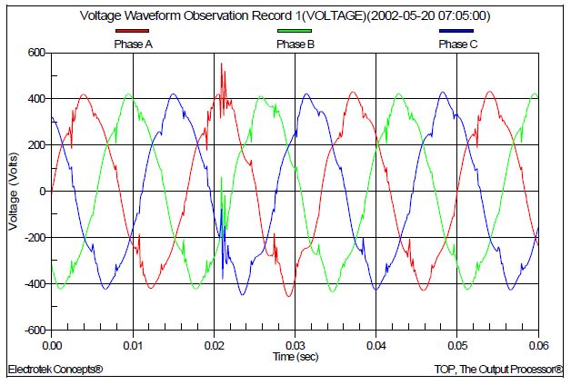
A viewing program that is capable of reading, displaying, and manipulating PQDIF and COMTRADE files is required for processing the power quality waveforms that are presented in this case study. A free program TOP, The Output Processor® [4] has this capability. The program is widely used in the utility industry for visualizing data from a variety of simulation and measurement sources. Figure 1 shows an example power quality event waveform signature that was measured using a Dranetz-BMI 8010 PQNode. The waveform shows the three-phase voltage on a 25 kV distribution feeder during a SiC arrester failure.
Figure 1 – Example of a Power Quality Event Waveform
REPRESENTATIVE POWER QUALITY WAVEFORM SIGNATURES
Power quality monitoring is used to characterize variations at various locations on utility and customer power systems. The length of the monitoring period is generally dependent on the nature of the power quality problem. For example, utility capacitor bank switching transients may be collected in several days, while harmonic distortion levels may need to be monitored for weeks, months, or even years to show the influence of load and seasonal variations. The current industry trend for power quality monitoring is fixed instruments that continuously monitor the power system.
Generally, it is advisable to begin monitoring as close as physically possible to the sensitive equipment being affected by the power quality variations. It is important that the monitor sees the same variations as the sensitive equipment. High-frequency transients, in particular, can be significantly different if there is significant separation between the monitor and the affected equipment. Another important monitoring location is the main service entrance. Transients and other voltage variations measured at this location can be experienced by all of the equipment in the facility. This is also the best indication of disturbances caused by the utility system (it is possible that disturbances at the service entrance are caused by events occurring within the facility). Monitoring site selection for diagnostic or evaluative monitoring is usually straightforward, being indicated by customer complaints, equipment failure reports, and other external factors.
This section includes a number of representative waveforms for various power system fault and power quality events, including voltage sags, momentary interruptions, voltage swells, harmonics, capacitor switching transients, transformer energizing transients, and ferroresonance. These waveforms all fall into one of the categories provided in IEEE Std. 1159-1995 (refer to Table 1) and are stored using either the PQDIF or COMTRADE formats. Each waveform includes background information regarding the source (e.g., measurement or simulation), cause, related utility or customer problem, and common solution.
Figure 2 shows a three-phase voltage sag waveform measurement for a remote three-phase fault on a distribution feeder. The magnitude of the resulting sag was approximately 60% for 9 cycles. The instantaneous voltage measurement was captured using a Dranetz-BMI 5530 DataNode and stored using the IEEE PQDIF file format. The customer power conditioning options for this event include UPSs and CVTs. The keywords for the waveform include sag and fault, while the slang terms that should be avoided include glitch, blink, wink, and outage.
Figure 2 – Remote Three-Phase Fault Voltage Waveform
Figure 3 shows a voltage rms trend during a distribution feeder momentary interruption sequence. The multiple reclosing interruptions, which are shown in per-unit, lasted approximately 1.2, 9.0, and 22.5 seconds respectively. The measurement was captured using a Dranetz-BMI 8010 PQNode and stored using the IEEE PQDIF file format. The customer power conditioning options for this event include UPSs and CVTs. The keywords for the waveform include interruption and fault, while the slang terms that should be avoided include glitch, wink, and outage.
Figure 3 – Reclosing Sequence during a Distribution Feeder Fault
Figure 4 shows a measured feeder voltage swell that occurred on the unfaulted phases close to a single line-to-ground fault on an overhead 34.5 kV distribution feeder. The swell was approximately 150%. The instantaneous voltage measurement was captured using a Dranetz-BMI 8010 PQNode and stored using the IEEE COMTRADE file format. The customer power conditioning options for this event include UPSs and CVTs. The keywords for the waveform include swell and fault, while the slang terms that should be avoided include glitch and surge.
Figure 4 – Voltage Swell on a Distribution Feeder
Figure 5 shows a measured 13.8 kV, 740 amp fundamental, 0.75 displacement power factor arc furnace load current. The waveform is an 18-cycle snapshot of one operating point for the furnace. The instantaneous current measurement was captured using a Dranetz-BMI 5530 DataNode and stored using the IEEE PQDIF file format. The power conditioning options for this event include harmonic filters and SVCs. The keywords for the waveform include current distortion, while the slang term that should be avoided is dirty power.
Figure 5 – Arc Furnace Current
Figure 6 shows the voltage on a customer secondary bus with moderate notching and distortion (VTHD ≈ 9%). It also shows a transient that was due to utility capacitor bank switching. The instantaneous voltage measurement was captured using a Dranetz-BMI 5530 DataNode and stored using the IEEE COMTRADE file format. The customer power conditioning options for this event include inductive chokes, and harmonic filters. The keywords for the waveform include notching and resonance, while the slang term that should be avoided is dirty power.
Figure 6 – Customer Voltage Notching
Figure 7 shows a 13.8 kV feeder current before-and-after energization of a 900-kVAr pole-mounted capacitor bank that creates a harmonic resonance that increases the current distortion (ITHD ≈ 13%). The instantaneous current measurement was captured using a Dranetz-BMI 8010 PQNode and stored using the IEEE PQDIF file format. The power conditioning options for this event include arresters and harmonic filters. The keywords for the waveform include capacitor and resonance, while the slang terms that should be avoided include surge, glitch, and spike.
Figure 7 – Feeder Capacitor Bank Switching and Harmonic Resonance
Figure 8 shows a 4.16 kV bus voltage waveform during utility capacitor bank switching. The resulting transient voltage was 1.35 per-unit, while the steady-state voltage rise was 1.2%. The instantaneous voltage measurement was captured using a Dranetz-BMI 8010 PQNode and stored using the IEEE PQDIF file format. The power conditioning options for this event include overvoltage control and arresters. The keywords for the waveform include oscillatory transient and overvoltage, while the slang terms that should be avoided include surge and spike.
Figure 8 – Substation Capacitor Bank Switching
Figure 9 shows a measured bus voltage waveform during a multiple restrike event on a 34.5 kV capacitor bank. The worst-case transient voltage was approximately 1.55 per-unit. The instantaneous voltage measurement was captured using a Dranetz-BMI 8010 PQNode and stored using the IEEE COMTRADE file format. The power conditioning options for this event include arresters. The keywords for the waveform include restrike and overvoltage, while the slang terms that should be avoided include surge and spike.
Figure 9 – Capacitor Bank Switch Multiple Restrike
Figure 10 shows the inrush current waveform for a distribution transformer energizing. Transformer inrush current typically decays over a period of about one second. The instantaneous current measurement was captured using a Dranetz-BMI 5530 DataNode and stored using the IEEE COMTRADE file format. The power conditioning options for this event include overcurrent protection, fuses, and reclosers. The keywords for the waveform include transient and overcurrent, while the slang terms that should be avoided include surge, and spike.
Figure 10 – Feeder Transformer Energizing
Figure 11 shows a phase-to-phase feeder voltage during a ferroresonance event that was caused by an unbalanced switching operation. The peak voltage was approximately 1.42 per-unit. The instantaneous voltage measurement was captured using a Dranetz-BMI 8010 PQNode and stored using the IEEE COMTRADE file format. The power conditioning options for this event include three-phase switches and secondary loads. The keywords for the waveform include ferroresonance and overvoltage, while the slang term that should be avoided is surge.
Figure 11 – Ferroresonance on Distribution Feeder
Figure 12 shows the simulated voltage waveform for a distribution system ferroresonance event on a 13.8 kV feeder. The peak voltage is approximately 2.89 per-unit. There were no arresters included in the model. The instantaneous voltage was created using an EMTP program and stored using the IEEE COMTRADE file format. The power conditioning options for this event include three-phase switches and secondary loads. The keywords for the waveform include ferroresonance and overvoltage, while the slang term that should be avoided is surge.
Figure 12 – Distribution Cable/Transformer Ferroresonance
SUMMARY AND CONCLUSIONS
Power quality problems encompass a wide range of disturbances and conditions on utility and customer systems, ranging from very fast transients to long duration outages. Problems also include steady state and intermittent phenomena, such as harmonic distortion and voltage flicker. This wide range of conditions makes the development of standard measurement and analysis procedures difficult. It is therefore beneficial to characterize power quality measurements and their related problems into common categories using standard data formats.
This case study includes a summary of power quality categories and characteristics. These characteristics and attributes are useful for evaluating measurement equipment requirements, system characteristics affecting the power quality variations, and possible measures to correct power quality problems.
This case study also includes an introduction to the commonly used data interchange formats PQDIF and COMTRADE and a collection of representative waveforms for various power system fault and power quality events. Each waveform includes a brief summary regarding the source (e.g., measurement or simulation), cause, related utility or customer problem, and common solution. Keywords and slang terms that should be avoided are also included with each waveform.
REFERENCES
IEEE Std. 1159-1995, IEEE Recommended Practice on Monitoring Electrical Power Quality, ISBN 1-5593-7549-3.
IEEE Std. 1159.3-2003, IEEE Recommended Practice for the Transfer of Power Quality Data, ISBN 0-7381-3578-X.
IEEE Std. C37.111-R2005, IEEE Standard for Common Format for Transient Data Exchange (COMTRADE) for Power Systems, ISBN 0-7381-1666-1.
Published by M.Sc Marko Pikkarainen, M.Sc Pekka Nevalainen, Dr. Pertti Pakonen, Prof. Pekka Verho, Tampere University of Technology, marko.pikkarainen@tut.fi
ABSTRACT
Two matters have strongly affected use of energy in Finland during recent years. The one is the greenhouse effect and the other is the energy price which has risen. These points have brought to the market many new devices that are more energy efficient, for example, heat pumps and energy saving lamps. Also the reduced manufacturing costs of devices have brought new kinds of loads available in the market. These new devices have changed the usage of electricity and usage of the distribution network. The distribution network has been designed to fulfil different kind of electricity usage need. That is why more power quality problems may occur in the distribution network in the future.
This paper will describe some power quality problems caused by the usage of ground source heat pumps and a wood splitter. This examination is based on the measurements that have been carried out in the real distribution network at low voltage level in Finland.
The examination showed that power quality problems may appear when using these typical new loads. Especially one big problem is a starting current of a wood splitter. Because of high starting current the voltage will drop and it may cause flicker.
I. INTRODUCTION
During recent years, the use of energy has changed because new kinds of loads have been connected to the distribution network. Three main issues have driven this change of loads. One is the green house effect and second is the energy price, which has risen, and third is the reduced manufacturing costs of devices.
The main act in preventing the green house effect and global warming is to decrease carbon dioxide emissions. Because of this more and more loads, which are reducing carbon dioxide emissions, have entered the market. For example compact fluorescent lamps are one group of such loads. Replacing incandescent bulbs with compact fluorescent lamps is one such act that should reduce carbon dioxide emissions because of the efficient light produce of compact fluorescent lamps compared with incandescent bulbs. The result of European Commission Regulation number 244/2009 is that incandescent bulbs will be gradually phased out from the market. [1, 6]
The increasing energy price has affected the use of energy so that customers have invested in devices which reduce costs and energy consumption. One good example of this kind of behavior is to replace an oil heating system with a heat pump or to add an air-to-air heat pump in complement electric heating. In Finland support from government has speeded up this change [4]. Figure 1 shows the number of installations of different types of heat pumps in Finland during the years 1996-2008. As shown in Figure 1 the number of heat pumps has grown very rapidly during past few years [2]. The growing trend has been the same all over Europe. The overall percentage of heat pumps of all heating types is not very massive in Europe but for example in Sweden heat pumps are the most common heating system in single-family houses with an approximately 34 % share of all. [3]
Figure 1. Number of installations of different heat pump types in Finland during years 1996-2008.[2]
Different heat pumps may have different effects on electrical energy consumption and to the way electricity is used. For example, if an oil heating system is replaced with a ground source heat pump, the overall consumption of electrical energy of a house will increase, but if an air-to-air heat pump is added to complement electric heating the consumption will decrease. However in both cases if the earlier consumption of the primary energy source is compared with the new consumption of electrical energy the consumption is decreased because most of the heating energy of heat pump is coming from ground or from air. Because of decreased overall primary energy consumption also carbon dioxide emissions are decreased depending on how electricity is produced. The greater usage of fossil fuels in electricity production the greater cutting can be achieved using heat pumps.
Heat pumps are a good example of loads which have become more common because of technical development and reduced manufacturing costs. Nowadays in Finland an air-to-air heat pump costs about 1200-3500 € including installation which is quite feasible price in Finland [5].
Ground source heat pumps cost more because it will need a ground circuit and the device is bigger in the power scale. Another example of a load which is becoming more and more common because of a cheap price is a wood splitter. Wood splitters are used for splitting thick woods to smaller ones so that woods can be used in fireplaces or in sauna stoves. Especially the cheaper versions of wood splitters that are designed for regular customers are very tempting devices because of the easiness of wood splitting.
These new loads are changing the use of electrical energy. Even though these loads may have a favorable effect on overall energy consumption some power quality problems may occur when using these loads. This is mainly caused by the new electrical characteristics of these loads. The planning principles of distribution networks are becoming old-fashioned and do not always fulfill the requirements of these new loads. From the power quality point-of-view the trickiest part will be the commonness of these loads because it means that power quality problems are also becoming more common.
This paper will study some power quality problems caused by the use of ground heat pumps and wood splitters. Devices have been selected to this study based on power quality complaints received by one distribution utility. The study is based on practical case study measurements which were carried out in real distribution networks in Finland. In the paper there is first a theoretical examination about power quality problems and previous mentioned loads. This is followed by a description of case study measurements carried out. Finally there are results and conclusions of those measurements.
II. THEORETICAL BACKROUND OF POWER QUALITY
Power quality is defined as “Set of parameters defining the properties of power quality as delivered to the user in normal operating conditions in terms of continuity of supply and characteristics of voltage (symmetry, frequency, magnitude, waveform)” [7]. In this paper, we are observing power quality in terms of quality of voltage. The limits for voltage quality are defined in standard EN 50160 Voltage characteristics of electricity supplied by public distribution networks. The standards object is to define and describe characteristics of the supply voltage concerning: frequency, magnitude, wave form and symmetry of the line voltages. “These characteristics are subject to variations during normal operation of the system because of changes of load, disturbances generated by certain equipment and the occurrence of faults which are mainly caused by external events”. Variation of the characteristics is random in time and location. Therefore on small number of occasions the limits can be expected to be exceeded. [8]
The standard EN 50160 defines the characteristics of voltage in low voltage and medium voltage networks [8]. Because we are interested power quality problems caused by devices which are connected to low voltage networks only the characteristics of voltage in low voltage networks are considered in this paper. The examination is focusing on a flicker caused by rapid voltage changes, voltage levels and voltage dips because those are a very common cause for power quality complaints as shown in Figure 2. Figure 2 presents the distribution of power quality complaints in one distribution utility in Finland during the years 2003-2005. About 70 % of all power quality complaints were caused by voltage changes.
Figure 2. Distribution of power quality complaints in one distribution utility in Finland during years 2003-2005 [9]
The other reason to focus only on flicker and voltage levels, when studying power quality, is that devices very commonly cause these disturbances. This mainly happens because a device requires power to operate. In addition voltage, a device will need current from the grid. This current will cause a voltage change over the impedance of a distribution network. This is seen in Equation 1. Depending on the connection of a device it may have different effects to phase voltages. If the connection is a three-phase connection and connection is symmetrical, all phase voltages will experience the same kind of effect voltage drop or voltage rise. If the connection is a single-phase connection, every phase will experience different kind of voltage change because of the star point displacement for example one could rise and the others drop.
where
ΔU = vector of voltage change ZN = vector impedance of distribution network IDEV = vector device current
The standard EN 50160 defines permitted levels for a flicker so that 95 % of long term flicker severity in any week should be lower or equal than 1. For voltage levels, standard defines that 95 % of the 10 min mean r.m.s. values of the supply voltage shall be within the range of Un ± 10 % during each one period and all of 10 min mean r.m.s. values shall be within range -15 % < Un < +10%. Exceptions for voltage levels can appear for example in remote areas with long feeder lines or not connected to a large interconnected network. In these cases voltage levels could be outside previous mentioned range but a customer or user should be informed of the conditions. [8]
III. THEORETICAL BACKROUND OF HEAT PUMP AND WOOD SPLITTER
In both devices, heat pumps and wood splitters, the source of power comes from induction motor. This component is the most significant component in these devices from the current usage and power quality point-of-view. In wood splitters the motor is usually a single phase induction motor. In heat pumps the motor can be either a single phase or a three phase induction motor. The connection type varies with different type of heat pumps. In bigger heat pumps, ground source heat pumps and air-to-water heat pumps, the induction motor is three-phase connected. In others heat pumps the induction motor is typically single-phase connected, because those heat pumps are smaller.
The biggest impact of an induction motor on the distribution network appears when the motor is started. The induction motor takes a high starting current. High starting current causes voltage change over the impedance of the distribution network. This phenomenon is seen in Figure 3 and equation 2. Figure 3 a presents an equivalent circuit of a polyphase induction motor and figure 3 b presents an approximate equivalent circuit of a polyphase induction motor. The approximate equivalent circuit is based on assumptions that the reactive component of impedances z1 and zm is much greater than the resistive component and the voltage E2 is only little smaller and nearly in the same phase with voltage V. These assumptions are valid in conventional induction motors in the normal running range. Equation 2 can be defined from figure 3 b. From Equation 2 can be seen that when the slip of the induction motor is small the motor takes a high current from a network. The slip is 1 at the moment of starting the induction motor and will decrease close to 0 after a starting. Single phase induction motors have a different equivalent circuit and equation for current taken from network compared to polyphase induction motors. Nevertheless the high starting current effect is similar to that in polyphase motors. [10]
Figure 3. a) Equivalent circuit of three-phase induction motor b) Approximate equivalent circuit of a three-phase induction motor [10]
r1 = resistance of stator x1 = leakage reactance of stator xm = magnetizing reactance r2 = resistance of rotor x2 = leakage reactance of rotor s = slip of motor
The starting current causes remarkable power quality problems when using induction motors because current reaches highest value at the beginning of start up and it won’t fluctuate much during normal operation. From power quality point-of-view, the critical factor is how often the motor is needed to start up. If the start up frequency is very high more voltage changes will appear. For the heat pumps length of the running cycle depends on the need of the heating energy, the dimensioning and parameter settings of a heat pump. If the heating power demand is close to the nominal heating power of the heat pump, the pump may run long times continuously. If the heating power need is clearly lower than the nominal heating power of the heat pump, stopping and reclosing of the pump will appear. The time between the stopping and reclosing the pump depends on the restrictions of the process and, for example, for one ground source heat pump the shortest time between stopping and restarting the process is 10 minutes according to a heat pump supplier.
For wood splitters starting up frequency varies depending on the operation logics of the device. Basically there are two operation logics to move hydraulic piston of the wood splitter. One is to perform all piston movements with hydraulic control when the induction motor is running. The other is to do the pressing with a hydraulic control when the motor is running and the backward movement with a spring when the motor is stopped. Second logic means that the repetition frequency of starting ups will be very high. In our measurements we had a wood splitter that needed to start up again every time a new wood was split.
IV. DESCRIPTION OF PRACTICAL CASE MEASUREMENT STUDY
In our study, two practical case measurements were made in Finland one in Lempäälä and the other in Tampere. In both cases the scope and the environment were bit different. Dranetz PX-5 power quality analyzer and Dranetz 4400 power quality analyzer were used as measuring devices in our study. In this chapter both practical case measurements will be described in depth.
Lempäälä rural area network
In Lempäälä the scope of the study was to explore power quality problems caused by a wood splitter in a rural area network. The wood splitter was single phase device and the nominal power of induction motor of the wood splitter was 2.2 kW. Operation logic of this wood splitter was that it needed to start up again every time a new wood was split. Feeders in this low voltage network were mainly aerial bundled cables called AMKA with cross-sections from 70 mm2 to 35 mm2 and the rated power of the 20/0.4 kV transformer feding the low voltage network was 200 kVA. In this low voltage network computational single phase short circuit currents at customers varied from 1400 A to 148 A. We decided to study power quality problems caused by a wood splitter in three locations in which measured single phase short circuit currents were 146 A, 275 A and 350 A at customer supply terminal. There were 10 m extension cord between a customer supply terminal and a plug point of a wood splitter so single phase short circuit currents were 136 A, 200 A and 233 A at a plug point of device. Figure 4 A shows an overall picture of low voltage network in Lempäälä. Measuring locations were situated along feeders 1 and 2. When a wood splitter was operated measurements were made in three places: one in a plug point of device, one in a customer supply terminal and one near the transformer. In addition when the wood splitter was operated in the location where the short circuit current was 146 A measurements were performed also in the location with a short circuit current of 275 A because those were located along the same feeder. Measured quantities were voltage and current waveforms and quantities defined in standard EN 50160 with an exception that a measuring period of short term flicker severity was 5 min.
Figure 4. A) Overall picture of a low voltage network in Lempäälä. B) Overall picture of the low voltage network in Tampere with measuring point locations
Tampere urban area network
In Tampere the scope of the study was to explore power quality problems caused by ground source heat pumps in an urban area network. Feeders in this low voltage network were mainly underground cables with cross-sections from 300 mm2 to 120 mm2 and the rated power of 20/0.4 kV transformer was 315 kVA. In this low voltage network computational single phase short circuit currents varied from 9,7 kA to 445 A and three phase short circuit currents varied from 10.8 kA to 1110 A so the network was quite strong. At the one end of this low voltage network two terrace houses changed their shared oil heating system into a separate ground source heat pump systems. The installation was made so that two ground source heat pumps, nominal heating powers 25 kW and 36 kW and maximum electrical powers 9,9 kW and 13,2 kW, were installed to both terrace houses. Starting of all heat pumps was direct on line starting so every time heat pumps were started a high starting current appeared. This place was selected to this study because some customers in both terrace houses complained about flicker. Overall picture of low voltage network, customer supply terminal short circuit currents and measuring points are illustrated in figure 4 B. Measured quantities were voltage and current waveforms and quantities defined in standard EN 50160.
V. PRACTICAL CASE STUDY RESULTS
This chapter presents the results of practical case studies. This chapter is headlined similarly as the previous chapter so that it is easy to follow results.
Lempäälä rural area network
Power quality problems caused by a wood splitter were remarkable at the customer end. Every wood splitting produced high starting current compared with the short circuit current and a remarkable voltage dip in the phase in which the wood splitter was connected at the customer supply terminals. This is why the biggest problems appeared in flicker and in number of voltage dips. The waveform and the RMS value of a starting current of one start up of a wood splitter are illustrated in Figure 5.
Figure 5. Waveform and RMS value of one start up of a wood splitter in place where a short circuit current at customer supply terminal was 275 A
It was detected that phase voltages of other phases than the phase in which the wood splitter was connected were raised at a customer supply terminal. This is due to a star point displacement of low voltage network when using single phase devices as predicted in Chapter 3. This effect is illustrated in Figure 6. Figure 6 shows phase voltages at customer supply terminal during start up of a wood splitter. Because of this effect power quality problems also appeared in other phases than the phase where a wood splitter was connected. Also Figure 6 shows that the phase voltage in connection phase drops so dramatic that every start up produced a voltage dip according to standard EN 50160 [8].
Figure 6. Phase voltages in place where short circuit current was 275 A at a customer supply terminal during start up of a wood splitter
Overall network impact results of practical case study in Lempäälä at customer supply terminal are summarized in Table 2. In measurements 1 and 3 the wood splitter was connected in phase L2 and in measurement 2 the wood splitter was connected in phase 1. Table 2 shows very dramatic short term flicker severity index increase at customer supply terminal in every phase when using the wood splitter at a customer installation. This means very annoying flicker and it also means that even short use of a wood splitter will exceed the limit Plt=1 in long term flicker severity calculated with definition in standard EN 50160 [8]. It should be noticed that an electrical chainsaw was used at same time when the wood splitter was operated. This increased little a short term flicker severity index. The effect of an electrical chainsaw to phase voltage was clearly smaller than the effect of a wood splitter.
Table 2. Overall results of a practical case study in Lempäälä
In addition of Table 2 results it was noticed that when the wood splitter was operated in measurement place 1 also power quality problems were recorded in measurement place 2. Geographical distance between these two places was 250 m. Operation of the wood splitter raised the short term flicker index of the other measurement place up to 7,2 in phase where a wood splitter was connected and up to 2,8 and 1,1 in other phases even though a wood splitter was operated in measurement place 1. Even though remarkable power quality problems appeared at customer end no power quality problems appeared at transformer. One way to prevent power quality problems mentioned in this chapter is to use only wood splitters of which piston movements are controlled with hydraulic control while the induction motor is running continuously.
Tampere urban area network
In Tampere four heat pumps were operated in same low voltage network. The measurement period was one week. During this period the mean temperature of a day was 3…9 °C and at night the temperature fell under 0 °C. This meant that heating power need was not near heating capacity of pumps so start ups and stops of pumps should appear. Installations of pumps were made so that a bigger pump heated only a water circulation of radiators. A smaller pump heated mainly use water but could support a bigger pump to heat a water circulation of radiators. Because of a direct on line start up of pumps high starting currents were detected. Starting currents of bigger pumps were 220…230 Arms and duration approximately 4 cycles. Starting currents of smaller pumps were 185…195 Arms and duration approximately 3 cycles.
Running cycle of pumps varied between terrace houses. Bigger pump of customer 1 ran typically from 1 h to 3 h 20 min. Time between two start ups varied from 1 h 40 min to 4 h 10 min and the average time between two start ups was 2 h 20 min. The total number of start ups was 73. Bigger pump of customer 2 ran typically from 50 min to 11 h. Start up times of bigger pump of customer 2 varied from 2 h 20 min to 12 h 10 min and the average time between two start ups was 3 h 50 min. The total number of start ups was 43. In both cases the biggest running times appeared at night time and shorter ones at day time. This is due to bigger heating need at night time. The differences between running times of bigger pumps could result from different size of houses and different heating system specifications.
Because the current measurements were placed in the common feeder of two different sized heat pumps, running times of smaller pump were difficult to determine. Start up times could still be determined. For the smaller pump of customer 1 time between two start ups varied from 19 min to 2h 10 min and the average time between two start ups was 39 min. The total number of start ups in one week was 255. For the smaller pump of customer 2, time between two start ups varied from 24 min to 1 h 40 min and the average time between two start ups was 30 min. The total number of start ups in one week was 371.
The total number of different heat pump start ups at customer 1 in each hour during one week is shown in figure 7. The figure 7 presents the number of start ups so, that if a smaller pump of customer 1 has started up once every day between 8.00 am and 9.00 am the number for smaller pump of hour 8.00 will be 7. As shown in figure 7, start ups of the smaller heat pump most commonly occurred at evening and day time. At night time, the number of start ups of smaller pump decreased significantly. This happened because more water was used at day time and evenings than at night time. For the bigger pump there was no specific time for start ups, only there was less start ups at morning. This occurred because heat pump ran longer at morning. This was because of bigger heating power need due to decreased outside temperature. Because of this kind of distribution in start up times, there was lower long term flicker severity index at night than day time. The key issue of high short term flicker index was bigger pump start up time and common start ups in the same 10 minute period for both heat pumps of customer 1. Also if there was common start up in the same 10 minute period for heat pumps of customer 2, it raised short term flicker severity index above 1, which is the irritation threshold.
Figure 7. The total number of different heat pump start ups in each hour of customer 1 during one week
The total number of heat pump start ups at customer 2 in each hour during one week is shown in figure 8. There were more start ups of smaller pump for customer 2 than customer 1. The number of start ups remained quite high all day. There were only little less start ups at night time than at day time. For the bigger heat pump there were only a few start ups during whole week. This was because of long running times of the bigger heat pump. The long term flicker severity index got higher values at evening than at night time because of this kind of distribution of start up times of different heat pumps. For high short term flicker severity index the key issues were the same for customer 2 as for customer 1. The start up of bigger heat pump at customer 2 meant higher short term flicker severity index at customer 2 and if there was start up of both bigger and smaller heat pumps at customer 2 in the same 10 minute period short term flicker severity index got even higher. Also if there was start up of both heat pumps at customer 1 short term flicker severity index increased above 1. In Table 3 short term flicker severity indices are summarized at different customer ends when different heat pumps started up. Short term flicker severity indices are average 10 minute values of events mentioned in table 3. Table 3 shows previously mentioned cross disturbance from start up of heat pump of one customer to the short term flicker severity index of the other customer. Table 3 also shows the greater effect of the bigger heat pump start up to the short term flicker severity index.
Figure 8. The total number of different heat pump start ups in each hour of customer 2 during one week
Table 3. Average values of short term flicker severity index at different customer end when different heat pump is or pumps are started up
Even though there were sometimes relatively high short term flicker indices the long term flicker index never exceeded the level Plt = 1 during one week. The highest long term flicker severity index was 0.99 at customer 1. The standard EN 50160 defines the threshold level to the flicker so that “under normal operating conditions, in any period of one week the long term flicker severity caused by voltage fluctuation should be Plt ≤ 1 for 95 % of the time”. This also means that threshold defined in the standard was not exceeded.
Despite the fact that flicker did not exceed the threshold level of standard EN 50160, flicker from heat pump start ups was clearly visible. The start ups of heat pumps were easily seen from lighting. Some customers can be irritated from this kind of rapid voltage changes. Now in the distribution utility point of view it is easy to say, that no problems occurred and case is closed. But in the customers point of view there might be flicker problems so the result “there cannot be flicker” is not a good answer from customer service point of view. In this case the result was that the supplier of all these heat pumps will install softstarters to heat pumps.
VI. CONCLUSIONS
In this paper there were examinations about power quality problems caused by loads that are coming more and more common. The examination is based on practical case measurements made in real distribution network in Finland. Two groups of loads were selected to this examination: wood splitters and heat pumps.
Wood splitter, which nominal power of induction motor was 2.2 kW and which was single phase device, was selected to this examination. This wood splitter was operated in different locations in one rural area low voltage network in Finland. In this network calculated short circuit currents varied from 1.4 kA to 146 A. Measurement places were selected so that measured short circuit currents were 148 A, 275 A and 350 A at customer supply terminals. In these places the wood splitter caused lots of flicker problems because of a high starting current and because of operation logic which caused lots of start ups of induction motor of the wood splitter. Flicker problems occurred in all three phases because of the star point displacement due to operation of a single phase device. Flicker problems caused by the wood splitter extended also to nearby customers along the same feeder. One way to prevent these flicker problems is to accept in the market only wood splitters of which piston movements are controlled with hydraulic control while the induction motor is running continuously. In such a case there will be less start ups of the induction motor.
Power quality problems caused by heat pumps were studied in urban area network in Tampere. In urban area network there was four big heat pumps installed into two terrace houses. Here start ups of heat pumps caused short term flicker severity index increasing over irritation threshold 1. Also start ups of heat pumps in one terrace house increased the short term flicker index over 1 at the other terrace house so there was cross disturbance from one terrace house to the other. Even though the short term flicker index was sometimes over 1 the long term flicker index was always under 1 so from the standard point of view there was no flicker problem. Despite this every start up of heat pumps could easily be seen from lighting so someone could feel this to be irritating. In this case the result was that the supplier of the pumps will install softstarters to all heat pumps.
Published by Electrotek Concepts, Inc., PQSoft Case Study: General Reference – Using Simulations and Measurements in PQ Analysis, Document ID: PQS0309, Date: April 16, 2003.
Abstract: Simulations provide a convenient means to characterize power quality problems, predict disturbance characteristics, and evaluate possible solutions to problems. They should be performed in conjunction with monitoring efforts and measurements for verification of models and identification of important power quality concerns. The models required for the simulations depend on the system characteristics and the power quality variations being evaluated.
The specific power quality concerns that need to be evaluated will be different for each customer. A review of the electrical configuration, protection practices, types of equipment used by the customer, process requirements, and economic impacts of problems will lead to a list of concerns that need to be studied.
USING SIMULATIONS AND MEASUREMENTS IN POWER QUALITY ANALYSIS
Power quality concerns that need to be evaluated will be different for each utility and customer configuration. A review of the electrical configuration, protection practices, types of equipment used by the customer, process requirements, and economic impacts of problems will lead to a list of concerns that need to be studied. These concerns can include possible problems with both the utility system and customer facilities. Possible power quality problem categories include:
Voltage transients caused by circuit switching and load switching within the customer facility.
Harmonic distortion from the application of adjustable-speed drives or other nonlinear loads.
Transformer heating caused by harmonic current levels.
Transient voltage magnification at low voltage capacitor banks.
Sensitivity of adjustable-speed drives (ASDs) and control systems to utility capacitor switching transients.
Transients and notching associated with power electronic equipment operation.
Neutral conductor overloading due to harmonic producing loads in commercial installations.
Voltage flicker from arc furnace loads and arc welding loads.
Voltage sags due to faults on parallel circuits on the same distribution system or faults on the transmission system.
Momentary interruptions at industrial and commercial installations due to recloser operations on feeder circuit breakers.
Coupled voltages in customer facilities due to lightning transients on the primary distribution systems.
Identification of the particular concerns involved for an installation provides a focus for a simulation-based study. Development of a model for analysis of the problem is dependent on the frequency range of the power quality variations that need to be studied. The model can be for computer simulations, hand calculations, or application of simple rules. For example, analysis of voltage sags often requires modeling that includes the utility transmission system, while analysis of high frequency transients might only require a model for a very local part of the customer facility.
Monitoring requirements are also based on the particular concern involved. If harmonic distortion is a concern, monitoring of steady-state conditions with a harmonic analyzer is required. Analysis of disturbances requires a disturbance monitor. The duration of monitoring depends on how often the problems occur. Some problems with voltage sags or momentary interruptions might only occur a few times per year due to faults on the transmission system, while problems caused by capacitor switching might occur every day. Other voltage variations of interest will typically fall somewhere between these extremes.
Data Collection Process
A representation of the customer system and important parts of the utility system should be developed for preliminary analysis. This model can be used for preliminary simulations or analysis to predict power quality problems and evaluate possible solutions to problems. In cooperation with the customer, the data for the model is collected and compiled into a database for convenient reference during the study.
Important information includes:
1. Utility system characteristics: − Primary voltage − Short circuit / load levels − Feeder configuration and characteristics – underground/overhead − Transformer ratings / connections / impedances − Protection practices, switching procedures − Capacitor applications (locations, sizes, switching method and controls) − Arrester sizing and placement
3.Power conditioning equipment: − Surge suppressors (arresters, varistors, etc.) − Isolation transformers − Constant voltage transformers − Voltage regulators / power conditioners − UPS systems − Harmonic filters − Custom power devices (utility distribution system)
Computer Simulation Process
Simulations provide a convenient means to characterize power quality problems, predict disturbance characteristics, and evaluate possible solutions to problems. They should be performed in conjunction with monitoring efforts and measurements for verification of models and identification of important power quality concerns. The models required for the simulations depend on the system characteristics and the power quality variations being evaluated. The simulations fall into three major categories:
− Transient simulations are often performed using the Electromagnetic Transients Program (EMTP). There are a number of different versions and platforms available. This is a valuable tool for analysis of circuit switching operations, capacitor switching, lightning transients, and transients associated with power electronic equipment operation.
The most widely used program for transient analysis is the EMTP. This program is used to simulate electromagnetic, electromechanical, and control system transients in multiphase power systems. It was originally developed by Hermann Dommel at Bonneville Power Administration (BPA) during the late 1960’s. Since then, there have been significant developments by groups all over the world.
The EMTP is a general-purpose computer program for simulating high-speed transient effects on electric power systems. The program features an extremely wide variety of modeling capabilities encompassing electromagnetic and electromechanical oscillations ranging in duration from microseconds to seconds. Examples of its use include switching and lightning surge analysis, insulation coordination, shaft torsional oscillations, ferroresonance, and HVDC converter control and operations.
The EMTP is used to solve the ordinary differential and/or algebraic equations associated with an “arbitrary” interconnection of different electrical and control system components. The implicit trapezoidal-rule (second order) integration is used on the describing equations of most elements that are modeled by ordinary differential equations. The result is a set of real, simultaneous, algebraic equations, which is solved at each time-step. These equations are written in nodal-admittance form, and are solved by ordered triangular factorization.
Studies involving use of the EMTP have objectives that fall in two general categories. One is design, which includes insulation coordination, equipment ratings, protective device specification, control systems design, etc. The other is solving operating problems such as unexplained outages or equipment failures.
Currently, primary development and support for member utilities is coordinated by EPRI and the Development Coordination Group (DCG). Additional DCG/EPRI EMTP information may be obtained from: http://www.emtp96.com/.
Another version of the EMTP is the Alternative Transients Program (ATP). The ATP is the royalty-free version of the EMTP. ATP is distributed by the ATP User’s Group for your country. ATP licensing is free, and requires only that you agree to the licensing terms. Additional ATP information may be obtained from: http://www.ee.mtu.edu/atp/ and
− Harmonic investigations are typically performed using steady-state analysis techniques at the individual harmonic frequencies. In general, harmonic-producing loads can be modeled as harmonic current sources, and the simulations used to predict harmonic voltages and currents throughout the customer and utility systems. Overloading of neutral conductors, transformer heating considerations, resonances caused by capacitor applications, and harmonic currents injected onto the utility system can be evaluated in the simulations.
SuperHarm, a harmonic simulation program developed by Electrotek Concepts, Inc. as part of the EPRI HarmFlo+ Workstation, uses a steady-state frequency domain analysis. The solution technique is a direct admittance matrix solution. This method requires that the system admittance matrix be solved for each harmonic of interest. A nonlinear device is modeled as a shunt-connected constant current source. The magnitude and angle of current injected at each harmonic frequency is determined with a Fourier transformer of the device’s line current waveform. SuperHarm allows the user to input harmonic current sources without concern for the phase angle between the bus voltage and the fundamental current.
Most harmonic simulation programs in use throughout the world use the admittance matrix approach similar to the one utilized in SuperHarm. Examples include V-HARM (Cooper Power Systems), CYMHARMO (Cyme) and HARMZW (CEPEL).
− Variations in the fundamental frequency voltage can be evaluated with conventional steady-state analysis tools. Power flow programs give system voltages as a function of load levels on the system. Fault programs (short circuit analysis) can calculate system voltage profiles during fault conditions for analysis of voltage sag concerns.
Computer programs used to solve power flows are divided into two types – static and dynamic (real time). Most power flow studies for system analysis are based on static network conditions. Real time power flows are primarily used for optimization of generation, VAr control, dispatch, losses, and tie line control.
A power flow solution gives the voltages at all buses and the power flow in all branches for a given set of operating conditions. It represents a steady state in which the influential parameters are in balance and a solution has been found. A power flow study is a collection of such solutions made when certain equipment parameters are set at different values.
Power flow/stability program vendors include EPRI, PTI (PSS/U), BPA/WSCC, Power Computing Associates, General Electric, Philadelphia Electric, ABB, and CYME.
There are numerous short circuit programs that can be used for power quality investigations. The full list given above for power flow/stability programs also provides short circuit programs. An addition to the list is ASPEN OneLiner. This program includes a special feature that allows convenient evaluation of voltage sag area of vulnerability.
In general, a process of developing a simple system model and working towards a more complete (and often more complex) model for an overall analysis yields the best results. A simplified system model allows the user to develop an understanding of the phenomena of interest. In addition, data verification is more efficient using this method. Once an understanding has been developed and the initial model has been verified, the user can then expand the system model to include more components. The overall study is then performed and solutions to the particular problem may be developed and analyzed.
Monitoring Process
The utility and customer systems being evaluated should be monitored to characterize the power quality variations and to verify the analytical models developed for simulations. The measurement program should be designed based on initial simulation results and on the particular sensitive loads existing at the customer facility. Monitoring will typically be performed on the feeder, at the customer service entrance, and close to the sensitive load. This will permit characterization of disturbances originating on the utility system and disturbances that are localized at the load. A measurement program plan should be developed which specifies:
− quantities to monitor − monitoring durations − threshold levels which will trigger recording of disturbances − waveform sampling and data storage requirements − analysis procedures and data presentation formats
Available monitoring instruments should be evaluated for the measurements required. The problem of obtaining adequate representation of both harmonic and transient conditions must be addressed in particular, if both of these concerns exist at a facility.
A customer site survey should be part of the measurement program design. The site survey should characterize the wiring and distribution system integrity and provide basic information about circuit and equipment loading. The site survey should also include discussions with facility personnel regarding characteristics of equipment problems and known customer system conditions at the time power quality variations have occurred.
The actual monitoring effort requires close cooperation between the customer and utility personnel. Monitoring sites and instrumentation should be selected based on the particular concerns being characterized. The duration of monitoring effort will depend on the parameters that can affect the power quality concerns. It is likely that the customer will need to be responsible for verifying that the monitor is operating properly on a day-to-day basis. The monitoring results should be compiled and analyzed for verification of analytical models and to provide a concise description of the possible concerns.
Selecting the Appropriate Monitoring Equipment
Power quality problems encompass a wide range of disturbances and conditions on the system. They include everything from very fast transient overvoltages (microsecond time frame) to long duration outages (hours or days time frame). Power quality problems also include steady-state phenomena such as harmonic distortion, and intermittent phenomena, such as voltage flicker. This wide variety of conditions that make up “power quality” makes the development of standard measurement procedures and equipment very difficult. Table 1 indicates the equipment requirements for identifying and monitoring specific power quality problems.
Table 1 – Equipment Requirements
Instrument Types
Although instruments have been developed that measure a wide variety of disturbances, a number of different instruments are generally necessary, depending on the phenomena being investigated. Basic categories of instruments that may be applicable include:
− Wiring and Grounding Test Devices − Multimeters − Oscilloscopes − Disturbance Analyzers − Harmonic Analyzers/Spectrum Analyzers − Flicker Meters
Transducer Requirements
Monitoring of power quality on power systems often requires transducers to obtain acceptable voltage and current signal levels. Voltage monitoring on secondary systems can usually be performed with direct connections but even these locations require current transformers (CTs) for the current signal.
Many power quality monitoring instruments are designed for input voltages up to 600Vrms and current inputs up to 5Arms. Voltage and current transducers must be selected to provide these signal levels. There are two important concerns that must be addressed in selecting transducers:
− Signal levels. Signal levels should use the full scale of the instrument without distorting or clipping the desired signal.
− Frequency response. This is particularly important for transient and harmonic distortion monitoring, where high frequency signals are particularly important.
EVALUATING RESULTS
The measurement results are analyzed in conjunction with the results of simulations to correlate customer problems with the utility system power quality levels. The initial measurements and the site survey are used to identify the phenomena involved and the important parameters. The subsequent measurement results are used to verify the model and characterize the actual power quality variations. Using this information, the model can then be used for more detailed simulations of possible solutions to the power quality problem. The simulations provide the means to evaluate a range of possible solutions from a technical point of view.
Once the range of technical solutions is identified, economic analyses need to be performed to evaluate the possible alternatives for solving customer power quality problems. These alternatives will generally include the following options:
− Power conditioning and/or filtering at the sensitive loads − Central power conditioning and/or filtering at the customer service entrance − Changing operating procedures or system design on the utility distribution system − Modification to the design of sensitive loads to make them less sensitive to power quality variations
The requirements for each of these options will be developed from the simulation effort and the analysis of measurement results.
Power conditioning in this case includes surge suppression, voltage regulation, and possibly backup for momentary interruptions. Harmonic filtering to solve harmonic problems can be applied either at individual loads or at the main service for a facility. Customer system design modifications, such as changing power factor correction procedures and equipment, can have an important impact on power quality variations. If particular loads are much more sensitive that other loads in the facility, either power conditioning at the particular load or design changes to the load equipment should be considered.
Momentary interruptions and voltage sags require careful consideration. Utility system modifications could include implementation of switching procedures to minimize transients associated with capacitor switching events or addition of current limiting devices to minimize the voltage sags that occur during faults on parallel feeders. The impact of protection practices on power quality levels experienced by customers should be evaluated carefully using both the analytical and measurement results.
SUMMARY
Simulations provide a convenient means to characterize power quality problems, predict disturbance characteristics, and evaluate possible solutions to problems. They should be performed in conjunction with monitoring efforts and measurements for verification of models and identification of important power quality concerns. The models required for the simulations depend on the system characteristics and the power quality variations being evaluated.
The specific power quality concerns that need to be evaluated will be different for each customer. A review of the electrical configuration, protection practices, types of equipment used by the customer, process requirements, and economic impacts of problems will lead to a list of concerns that need to be studied.
REFERENCES
Potential Transformer Accuracy at 60 Hz Voltages Above and Below Rating and at Frequencies Above Hz, D. A. Douglass, presented at the IEEE Power Engineering Society Summer Meeting, Minneapolis, MN, July 13-18, 1980.
Current Transformer Accuracy with Asymmetric and High Frequency Fault Currents, D. A. Douglass, IEEE Transactions on Power Apparatus on Systems, Vol. PAS-100 No. 3, March, 1981.
Transducer Performances for Power System Harmonic Measurements, C. J. Cokkinides, L. E. Banta, A. P. Meliopoulos, Proceedings of the International Conference on Harmonics, Worcester, MA, October 1984.
Computation of Current Transformer Transient Performance, IEEE Transactions on Power Delivery, Vol. PWRD-3 No. 4, October 1988.
Electrical Transients in Power Systems, Second Edition, Chapter. 18, A. N. Greenwood, John Wiley and Sons, New York, 1991.
RELATED STANDARDS IEEE Standard 1159 IEEE Standard 1346 IEEE Standard 1250 IEEE Standard 1036 IEEE Standard 519
GLOSSARY AND ACRONYMS ASD: Adjustable-Speed Drive CT: Current Transformer EMTP: Electromagnetic Transients Program HVAC: High-Voltage Air Conditioning MOV: Metal Oxide Varistor PF: Power Factor PWM: Pulse Width Modulation TVSS: Transient Voltage Surge Suppressors
Published by Electrotek Concepts, Inc., PQSoft Case Study: Customer Data Analysis, Document ID: PQS1102, Date: March 15, 2011.
Abstract: Monitoring is often used to characterize power quality levels at various locations on utility and customer power systems. Field measurements provide a convenient means to characterize power quality problems. This case study summarizes a commercial customer power quality measurement data evaluation.
CUSTOMER DATA ANALYSIS CASE STUDY
A commercial customer power quality measurement data analysis case study was completed for the system shown in Figure 1. The utility substation included a 10 MVA, 161 kV/12.47 kV step-down transformer and two 12.47 kV distribution feeders that supplied a mix of residential and commercial customers. One of the feeders had a switched 300 kVAr capacitor bank that was being used for power factor correction and voltage control. The monitoring location is identified as Commercial Customer #1. The customer, which was supplied from 150 kVA transformers with 120/208 V and 480 V secondary buses, was a small office building.
The twelve-month monitoring period was from January 1, 2003 thru December 31, 2003. The power quality instrument used to complete the power quality measurements was the Dranetz-BMI 8010 PQNode™. The instrument samples voltage at 256 points-per-cycle, current at 128 point-per-cycle, and follows the IEC 61000-4-3 method for characterizing harmonic measurement data. The sampling rate also allows characterization of low-to-medium frequency oscillatory transients. The measurement and statistical analysis was completed using the PQView® program.
Figure 2 shows the rms voltage histogram for the twelve-month monitoring period. Statistical analysis of the 37,463 individual steady-state measurements yielded a minimum voltage of 264.1 V, an average voltage of 294.4 V, and a maximum voltage of 306.3 V. In addition, the CP95 value was 299.7 V (108% of nominal). CP95 refers to the cumulative probability, 95th percentile of a value.
Figure 3 shows the measured customer voltage distortion (VTHD) trend during the twelve-month monitoring period. The minimum harmonic distortion was 0.79%, the average distortion was 2.56%, and the maximum distortion 21.18%. The CP95 value was 3.83%. The measured voltage distortion value was below the assumed 5% limit a vast majority of the time.
Figure 1 – Illustration of Oneline Diagram for Commercial Customer Data Evaluation
Figure 2 – Measured Customer Secondary Voltage Histogram
Figure 3 – Measured Customer Secondary Voltage Distortion
Figure 4 shows the statistical summary of total harmonic voltage distortion (VTHD) and number of individual harmonics for the twelve-month monitoring period. The analysis showed that the predominate harmonics for the measured customer secondary bus voltages were the 3rd, 5th, and 7th. The measured values were below the assumed 5% voltage distortion limit.
Figure 4 – Measured Statistical Summary of Voltage Distortion and Harmonics
Voltage sags and momentary interruptions are inevitable on the electric power system. Many of these variations occur during faults on the power system, and since it is impossible to eliminate the occurrence of faults, there will always be voltage variations on customer systems. Other sources of voltage variations include unbalance, induction motor starting, and voltage flicker. Table 1 shows an rms variation event summary listing for several of the sixty rms variation events that occurred during the twelve-month monitoring period. The table shows the date-and-time for each event, as well as the phase-to-neutral voltage magnitude in both volts (kV) and per-unit and the event duration in both seconds and cycles.
Figure 5 shows the corresponding waveform and rms characteristic for one of the voltage sag events measured during the monitoring period (Event #3 in Table 1). The magnitude of the voltage sag was 47.9% and the duration was 7.0 cycles. The voltage sag occurred during a storm. It was caused by a short-duration fault and subsequent fuse clearing on a feeder branch circuit.
Table 1 – Event Listing for Measured RMS Variations
Figure 5 – Measured Customer Secondary Voltage Sag Event
When there are a significant number of events, it is generally not desirable to show the results for each individual measurement. One method for summarizing rms variation event data is to graph the magnitude and duration data on one single scatter plot. This method may also include an equipment tolerance (e.g., ITIC) overlay. Figure 6 shows a summary of the measured rms variation events along with an ITIC overlay. The graph also shows the number of events that are outside the equipment sensitivity characteristic.
Voltage variation indices may be used to assess the service quality for a customer. One commonly used benchmarking value is known as SARFI, which stands for System Average RMS Variation Frequency Index. SARFI represents the average number of specified rms variation measurements that occurred over the assessed period. For example, SARFI70 is a measure of the number of voltage sags that can be expected with a minimum voltage below 70%. Another popular use of SARFI is to define the threshold as a curve. For example, SARFICMEBA would represent the number of rms variation events outside the commonly used CBEMA voltage tolerance envelope. The CBEMA curve was originally developed by the Computer Business Equipment Manufacturers Association. The curve was first published in IEEE Std. 446-1995.
The calculated SARFI values for the twelve-month monitoring period are summarized in Table 2. The SARFI90 value of fifty-six can be determined by counting the number of events with a voltage magnitude below 90%. In addition, the SARFIITIC value of twenty-four that is shown in the table corresponds to the data previously shown in Figure 6.
Table 2 – Summary of RMS Voltage Variation SARFI Values
The causes of the transients measured during the monitoring period included capacitor bank switching, transformer energizing, single-phase faults, switch failure, recloser operations, and current-limiting fuse operations.
Table 3 shows a transient event summary listing for several of the representative transients that were measured during the twelve-month monitoring period. There were several thousand oscillatory transients that were captured. The table shows the date-and-time for each event, as well as the peak phase-to-neutral voltage magnitude in both volts (kVpk) and per-unit and the event duration in both seconds and cycles.
Table 3 – Event Listing for Measured Transient Events
One of the common transient events measured throughout the monitoring period was during energization of the 300 kVAr capacitor bank on the utility distribution feeder. Figure 7 shows a representative measured three-phase customer secondary voltage waveform during uncontrolled energization of the pole-mounted 300 kVAr capacitor bank on feeder #1 (Event #3 in Table 3). The utility capacitor bank was switched on-and-off each day using time clock controls in an attempt to maintain a relatively constant voltage profile. The peak magnitude of the measured transient voltage was 591.1 V (1.51 per-unit) and the principal frequency for the capacitor energizing waveform was approximately 900 Hz. The duration of the transient event was approximately 8.203msec or 0.492 cycles. The capacitor bank was energized using a three-phase oil switch.
Typical voltage magnitude levels for switching distribution capacitor banks range from 1.3 to 1.5 per-unit and typical transient frequencies generally fall in the range from 300 to 1000 Hz. Power quality problems related to utility capacitor bank switching include customer equipment damage or failure, nuisance tripping of adjustable-speed drives or other process equipment, transient voltage surge suppressor failure, and computer network problems.
Utilities switch capacitor banks in-and-out of service routinely to provide voltage support and to improve power factor. One potential disadvantage of capacitor bank switching is the effect that such an operation can have on the topology of the system. Switching capacitor banks into mostly inductive circuits can tune the natural frequency of the circuit closer to harmonic frequencies that might be prevalent on the system. Obviously, this can be a significant problem, possibly resulting in severe voltage and current distortion, increased losses, and overheating of system equipment.
Figure 7 – Measured Customer Transient Voltage during Capacitor Bank Switching
Another relatively common transient event was during a fuse operation on one of the utility distribution feeders. A representative three-phase waveform is shown in Figure 8. The peak magnitude of the measured transient voltage was 593.8 V (1.52 per-unit) and the principal frequency for the transient waveform was approximately 300 Hz.
Figure 8 – Measured Customer Transient Voltage during Fuse Operation
Table 4 shows a summary of relevant terms and indices related to power quality problems on utility and customer power systems.
Table 4 – Power Quality Related Equations and Indices
SUMMARY
This case study summarized a commercial customer power quality measurement data analysis. The case showed that monitoring may be used to characterize power quality levels on customer power systems. The length of the monitoring period, which was twelve-months for this study, is dependent on the nature of the power quality problem. The analysis included trends and statistical summaries of the rms voltage and the harmonic voltage distortion levels.
The results showed that the harmonic voltage distortion levels were below the assumed 5% voltage distortion limit. The results of the analysis also showed that most of the rms variation events were short duration voltage sags. Constant voltage transformers, coil-lock devices, magnetic synthesizers, and a number of power electronic based power conditioners may be used for protection against voltage sag events. Voltage sag protection may be implemented on a single coil or piece of equipment. Correction may also be chosen for large portions of a facility or even for the entire facility.
Mitigation alternatives for reducing harmonic distortion levels include methods for modifying the power system to reduce or eliminate the harmonic resonances that can cause very high current or voltage distortion levels. For example, a passive shunt harmonic filter may be added to the utility or customer system to divert the troublesome harmonic currents off the system and into the filter.
The causes of the transients measured during the monitoring period included capacitor bank switching, single-phase faults, recloser operations, and current-limiting fuse operations. Customer transient mitigation options include power conditioners and TVSSs.
REFERENCES
IEEE Recommended Practice for Monitoring Electric Power Quality,” IEEE Std. 1159-1995, IEEE, October 1995, ISBN: 1-55937-549-3.
IEEE Recommended Practices and Requirements for Harmonic Control in Electrical Power Systems, IEEE Std. 519-1992, IEEE, ISBN: 1-5593-7239-7.
“IEEE Recommended Practice for Emergency & Standby Power Systems for Industrial & Commercial Applications” (IEEE Orange Book, Std. 446-1995), IEEE, ISBN: 1559375981.
“IEEE Guide for Application and Specification of Harmonic Filters,” IEEE Std. 1531-2003, IEEE, ISBN: 0-7381-3718-9.
“IEC Electromagnetic Compatibility Part 4-3: Testing and Measurement Techniques – Radiated, Radio-Frequency, Electromagnetic Field Immunity Test,” IEC 61000-4-3 Consol. Ed. 3.1-2008, International Electrotechnical Commission.
R.C. Dugan, M.F. McGranaghan, S. Santoso, H.W. Beaty, “Electrical Power Systems Quality,” McGraw-Hill Companies, Inc., November 2002, ISBN 0-07-138622-X.
RELATED STANDARDS IEEE Std. 1159, IEEE Std. 519
GLOSSARY AND ACRONYMS ASD: Adjustable-Speed Drive DPF: Displacement Power Factor PF: Power Factor PWM: Pulse Width Modulation THD: Total Harmonic Distortion TPF: True Power Factor
Addressing Evolving Customer Technologies and an Increasingly Complex Power Grid
Published by Electric Power Research Institute (EPRI), Inc. Document ID: 3002022396, March 2022.
Introduction
Over the past 50 years, the concept of power quality (PQ) has evolved from being an unknown and undefined concept to being understood as a fundamental component of grid performance, utility economics, and customer satisfaction.
Until the 1970s, most electrical loads were linear and could ride through most grid voltage and current variations. The emergence of microprocessors, process controls, and other equipment sensitive to voltage and current variations, as well as equipment that caused PQ variations, resulted in an entirely new technology discipline focused on the compatibility between the grid and the devices connected to it. This concept of compatibility is at the heart of PQ issues and research.
While industrial facilities may have the most significant PQ issues, PQ concerns can be important for any customer. For instance, voltage variations caused by large load variations, such as when motors start or when arc furnaces are in use, may cause lights to flicker for customers over a wide area. While light flickers are not as much of a concern these days with LED lights that have their own power supplies, voltage sags occurring over wide areas when there is a fault on the grid can potentially affect a diverse range of equipment and processes. Consumer electronic devices, like televisions, computers, and now electric vehicle chargers, can affect the grid and other customers by causing harmonic distortion.
These types of issues have been the subject of detailed laboratory and field investigations conducted by EPRI’s PQ research program since the 1980s in coordination with other investigators around the world. EPRI’s PQ research has helped raise awareness of this important topic while providing solutions to utilities. As EPRI celebrates its fiftieth anniversary in 2022, it is timely to take a short look at the history of the PQ research program and related activities in the industry as a whole new set of compatibility challenges emerge.
This white paper attempts to accomplish three things:
Provide a timeline and overview of selected historical PQ developments and events.
Offer a starting point for discussions on the topic. In examining this history, lessons learned may be useful when looking for solutions to current and future PQ issues.
Discuss new challenges in the increasingly complex grid environment associated with new technologies and system configurations that are characteristic of the energy transition.
A PQ problem is any power condition manifested in voltage, current, or frequency deviations that results in the failure or maloperation of customer equipment [8]. These problems can include transients, flickers, voltage sags and swells, and harmonic distortion.
The Concept of Compatibility
The concept of “compatibility” is key to virtually all PQ investigations. To achieve compatibility, one must understand the causes of PQ variations (or emissions) and how these can result in voltage variations that can affect other equipment (interaction of emissions with the system impedance characteristics). Equipment immunity levels must be selected to make sure that equipment can operate properly in the presence of “normal” PQ variations. System variations and equipment immunity levels are both probabilistic phenomena, so achieving compatibility is a probabilistic function as well (Figure 1). This concept of compatibility was best described as part of the International Electrotechnical Commission (IEC) 61000 series of standards, first drafted in the 1990s, which addresses the full range of PQ issues from emissions to immunity, from to measurements to testing. Much research has gone into trying to gain an understanding of the relationship between system variations and equipment immunity levels, the economics of PQ impacts, and solutions to problems when they arise.
Figure 1. The concept of compatibility levels as defined in IEC Standard 61000-3-2
Providing the Foundation
Research into PQ events starts with understanding the phenomena associated with PQ variations and impacts. A few of the industry leaders and the publications that resulted from their work are referenced here as foundational in creating a basic understanding
Francois Martzloff—National Institute of Standards and Technology
Early PQ problems often involved transient voltages from lightning and system switching affecting equipment, especially as electronic equipment started to become more common. Transient voltage measurements, transient protection, and grounding practices were implemented to avoid failures due to transient voltages. Francois Martzloff (Figure 2) at the National Institute of Standards and Technology (NIST) was a leader in characterizing these transient voltage concerns, determining how to measure them, and protecting equipment from them. In 1991, Martzolff pulled together state-of-the-art references on surge protection as part of NISTIR 4657 [1].
Figure 2. Francois Martzloff
This early work was sponsored by the key organizations that were already working on the range of PQ issues at the time, including:
Computer and Business Equipment Manufacturers Association (CBEMA)
EPRI
Institute of Electrical and Electronics Engineers (IEEE) Standards Coordinating Committee 22 on Power Quality
IEEE Surge Protective Devices Committee
Harmonics—Roger Dugan, Mack Grady, Erich Gunther, Mark Halpin
Concerns for distortion due to nonfundamental components of the voltage and current and the potential for resonances at these higher frequencies were understood since the beginning of alternating current systems. Charles Steinmetz [2] first described these concerns, which were soon to become known as harmonics. The mathematical foundation for characterizing harmonics goes back to Jean-Baptiste Joseph Fourier [3] and the concept of Fourier analysis to represent a signal by a superposition of its harmonic components. Harmonic concerns became more pronounced as electronic equipment became more prevalent in the 1980s. In this decade, major advances were made in harmonic analysis methods and in standards for evaluating compatibility (such as IEEE 519 and IEC 61000-3-2). Roger Dugan, working on an EPRI project in the late 1970s, developed one of the first harmonic analysis tools, in parallel to work at Purdue by Mack Grady. There have been many advancements to these tools over the years, in particular by leaders like Erich Gunther. Mark Halpin took this work and led its incorporation into standards.
Harmonics are sinusoidal voltage or current waveforms whose frequency is an integer multiple of the system frequency (60 Hz in U.S. systems). Periodically distorted waveforms, which often are results from the use of nonlinear loads, can be mathematically described as the sum of ideal waveforms of the fundamental frequency and its harmonics [27].
Voltage Sags—Tom Key, Math Bollen, Dan Sabin
Short-duration voltage variations, known as voltage sags, became one of the most important PQ concerns as industrial processes became automated and the controls for these processes began to include electronic equipment that could be affected by these short voltage variations. CBEMA did some of the early work in 1977 to define the concept of characterizing voltage sags by their magnitude and duration so that they could be compared with the ride-through characteristics of equipment. The CBEMA curve is discussed later in this white paper, including the coordination with Tom Key and the EPRI Power Electronics Application Center (EPRI-PEAC). However, these concepts were advanced significantly by Math Bollen, who wrote the book on voltage sags [4], and Dan Sabin, who developed analytical tools for analyzing PQ measurements that became part of standard utility PQ investigations.
Measuring Power Quality—Abe Dranetz, Alex McEachern
Characterizing PQ with measurements has been key for all types of PQ variations and understanding their impacts. Francois Martzloff, whose work was mentioned previously, led in characterizing variations. One of the first portable PQ measurement instrument that brought forth understanding of PQ issues was developed by Abe Dranetz [5]. Dranetz measurements soon became synonymous with PQ investigations. Alex McEachern took this concept to a new level, first with the Basic Measuring Instruments PQ monitor for portable measurements and then with the PQNode, which was the first device for permanent PQ monitoring with an overall data management and analysis platform called PQView (development led by Erich Gunther and Dan Sabin for the large PQ benchmarking project performed in the late 1980s and early 1990s).
Electrical Power Systems Quality Book—Mark McGranaghan, Roger Dugan, Surya Santoso
Much of this background and the advancements that followed have been documented in the multiple editions of the book Electrical Power Systems Quality (Figure 3). First published in 1996, with subsequent editions released in 2003 and 2012, this textbook has become the de facto textbook for studying PQ issues [6].
Figure 3. T he Electrical Power Systems Quality textbook
A Harbinger of Things to Come: Ben Franklin Brings Home His Point With the Lightning Rod
Coping with lightning long predates the electric power grid but figures prominently in the history of PQ. One of Benjamin Franklin’s most famous inventions was the lightning rod. In 1749, Franklin described the similarities he observed between electricity and lightning—that is, that both looked like light, appeared in forked arcs, crackled, and were able to kill animals [7]. He became determined to find a method of proving that lightning was in fact electricity.
In 1752, Franklin set out to perform an experiment to test his hypothesis that lightning was indeed electricity. One day as a storm moved in, he used a kite that consisted of a wire and silk handkerchief connected to a hemp string, metal house key, and silk string. The hemp string could grow wet from the rain, which meant it could conduct an electrical charge quickly. Using a Leyden jar, he was able to collect “electric fire”—stored electricity—from the key, thereby providing evidence that lightning was made of electricity.
Even since before the experiment with the kite and key, Franklin advocated for sharp-pointed lightning rods to protect public buildings (Figure 4). Franklin’s invention was seen as an effective deterrent to the scourge of fires from lightning strikes, as fewer damaging lighting strikes hit buildings equipped with lighting rods grounded to the earth. The lightning rod became a valuable tool to mitigate lightning damage and served as a harbinger for future developments in PQ.
Figure 4. Franklin’s lightning rod (Source: Franklin Institute)
Creating a Power Quality Research Program
The connection of more nonlinear loads to the grid in the 1980s and the unique customer issues that emerged prompted growing concern about PQ. Primarily affected were process oriented equipment and microcomputers sensitive to minor changes in the nature of electricity supplied. Initial investigations established a knowledge base, leading to basic definitions of PQ phenomena and uncovering the need for measurement, analysis, and benchmarking capabilities. Utilities began investigating customer PQ issues and educating customers on the basics of PQ. Utilities worked with customers and EPRI to collaboratively identify challenges and possible solutions. Over the years, this knowledge has been organized as part of the EPRI Power Quality Online Resource Center (https://mypq.epri.com/).
A technology transfer pipeline coalesced with utilities, customers, EPRI, and equipment manufacturers working together, and PQ emerged as a business. PQ monitoring advanced, allowing for the first instances of large-scale monitoring and benchmarking, accelerated with monitoring and data analytics developed for the EPRI Distribution Power Quality (DPQ) benchmarking initiatives [8], and resulted in significant accumulations of data used for postmortem analyses. From a business perspective, deregulation reduced the focus on customer equipment causing PQ issues and shifted to ensuring utility service did not cause customers issues. PQ standards continued to develop, covering more phenomena and in greater depth. The IEC emerged as a major force on the standards front. Key technology development included the dynamic voltage regulator and superconducting magnetic energy storage systems that could be the basis of enhanced PQ services demonstrated by American Electric Power [9] and Duke Energy [10].
The EPRI Power Electronics Application Center
The PQ research program at EPRI took off with the creation of the EPRI-PEAC in 1988. This center led equipment testing for compatibility, tested new solutions for PQ problems, developed new tools like the voltage sag generator for evaluating compatibility in customer processes, and helped coordinate conferences and publications that led the industry for many years. Leaders in this center included Tom Key, Arshad Mansoor, and Mark Stephens.
PQ Case Studies: Building the Understanding
One of the keys to creating an awareness and understanding of PQ issues was conducting actual investigations of problems and publishing these as PQ case studies. EPRI has collected more than 100 case studies focused on PQ solutions for utility customers in the Next Generation Online PQ Case Study Library (EPRI, 1002281).
Building a Worldwide Collaboration
As understanding of PQ issues was growing, industry conferences and workshops helped spread the word and build a collaboration that still exists today in this field. Three series of conferences were particularly important:
International Conference on Harmonics in Power Systems, later renamed as the International Conference on Harmonics and Quality of Power—Alex Emmanuel.
Power Quality magazine’s Power Quality Conference and John Mungenast Power Quality Leadership Award.
EPRI Power Quality Interest Group and Power Quality Applications conferences sharing case studies and research results from around the world. These conferences accelerated the adoption of compatibility solutions and tools.
Compatibility Means Economics
As the fundamentals of PQ became understood, it became clear that ultimately, PQ issues are economic issues. For example, if a PQ variation causes the shutdown of a semiconductor chip production process or an automotive production, the consequences can be in the millions of dollars. Evaluating the economics is a combination of forecasting the likelihood of a problem, understanding the impacts, and being able to describe potential solutions. Voltage sags were one of the initial areas where this became especially critical, and Math Bollen and Dan Sabin led in characterizing the problem, as described previously. It is also worthwhile to note the contributions of Larry Conrad in leading the work on IEEE 1346 [11] that focused on the economic evaluation and creating an understanding within the industrial community. The work on the economics of PQ continued in the International Council on Large Electric Systems (CIGRE) and IEC working groups and still continues to this day.
Uninterruptible Power Supply to the Rescue
By the 1930s, electrical power supply had become well established in cities and towns, with almost 90% of people living in urban areas having access to electricity [13]. Given this growing dependence on electricity for daily activities, many electrical engineers and inventors were likely trying to work out solutions to riding through the inevitable dips and interruptions in electrical supply. In 1932, a patent application was filed by John J. Hanley for an “Apparatus for Maintaining an Unfailing and Uninterrupted Supply of Electrical Energy,” a device that would become known as the uninterruptible power supply (UPS). Granted on April 3, 1934, the patent described an apparatus that could be used to change automatically from one source of electrical energy supplying an external circuit to another source of electrical energy with no interruption of electrical flow in the external circuit (Figure 5) [14]. The patent went on to describe how the invention could supply energy temporarily from a battery during the period of time after the main source of electricity had been interrupted and before the circuit had been opened to the new source of electrical energy. Further instructions describe the assembly of the unidirectional current valve needed for the apparatus and the design of an audible warning signal to indicate failure of the original commercial circuit.
The emphasis in the patent application was on maintaining “uninterruptedly and with unfailing certainty” the necessary electrical energy for alarms and signals, such as fire alarms and railway signal systems, “where the safety of property and human life depend upon the unfailing operation of the system.” In addition, mention is made of maintaining the lighting systems for hospital operating rooms and for theaters, the latter of which may have provided the original spark of inspiration for Hanley, given his background.
Whether the safety goals expressed in this patent were fueled by a particular calamity or failure in electrical supply is not known. At the time, according to Hanley’s patent, most fire-alarm systems relied on batteries or other sources of power rather than on a commercial power line. Hanley’s invention would have allowed more systems—not just fire-alarm systems, but railroad-crossing systems, traffic stoplights, burglar alarms, and newly invented smoke detectors—to safely take advantage of utility-supplied power.
Today, the UPS is one of the most ubiquitous PQ mitigation technologies. The largest UPS on record can power an entire city and surrounding communities for about seven minutes. The battery electric storage system in Fairbanks, Alaska, is bigger than a soccer field, weighs 1500 tons, consists of 13,760 liquid electrolyte-filled nickel-cadmium battery cells, and can discharge up to 46 MW [15]. On a much smaller scale, a 900-W UPS with digital display and colored lights is presently being marketed to gamers as a stylish all-in-one device for backup, surge protection, and automatic voltage regulation for personal computers, gaming devices, and peripherals.
There are varying options for protection in cases where voltage sags are the main issue, such as in many industrial processes.
Figure 5. John J. Hanley’s original design for an Apparatus for Maintaining an Unfailing and Uninterrupted Supply of Electrical Energy, a technology that would later become known as the uninterruptible power supply
Solutions to issues of voltage sags and momentary interruptions are key to the economic evaluation. These solutions started with a whole industry offering uninterruptible power supplies (UPS) with battery storage to provide ride-through capability. However, many other innovations, from simple protection of process controllers to new power electronic topologies (see, for example, leadership of Deepak Divan in developing novel solutions [12]), were developed and documented in the case studies shared with the industry.
SEMI F47 Standard Improves Compatibility with Many Process Industries (2000)
The semiconductor industry has been vital to the development of electronic devices. Started over 45 years ago, the Semiconductor Equipment and Materials International (SEMI) International Standards Program releases standards aimed at improving product quality and reliability at a reasonable price and steady supply [16]. SEMI F47, which sets equipment voltage sag immunity for the semiconductor industry, was developed through a coordinated effort among semiconductor manufacturers, equipment suppliers, and electric utilities, including many EPRI member companies. The effort began in EPRI’s System Compatibility Research Project Task 24, “Power Quality in Semiconductor Fabrication,” which, through industry collaboration, examined why semiconductor production equipment is susceptible to voltage sags. Task 24 workshops, research, and testing began in 1997, and a request for the establishment of a PQ standard for semiconductor tools was made following the September 1997 workshop in Tempe, Arizona [17]. In February 2000, SEMI F47 was published, defining the minimum voltage sag levels not to cause maloperations of semiconductor equipment. Initially, equipment manufacturers were hesitant to adopt the standard, but researchers showed how the standard could be met with minimum design impact. As a result of this standard being published and adopted, semiconductor customers saw fewer PQ issues, saving manufacturers millions of dollars annually [17].
EPRI’s Consortium for Electric Infrastructure for a Digital Society Report Documents the Economic Value of Power Quality
By 2000, the concept of monitoring and maintaining PQ had been well established as a need in a digital society. Industrial processes were becoming increasingly digitized, prompting greater sensitivity to disturbances in the power supply. Continuous process manufacturing was particularly susceptible as even a small disturbance could lead to lost product, damage, and difficult cleanup. For example, if production stops in injection molding factories, plastic could harden, leading to costly delays before production could resume. In 2000, EPRI’s Consortium for Electric Infrastructure for a Digital Society (CEIDS) report The Cost of Power Disturbances to Industrial and Digital Economy Companies provided a first-of-its-kind comprehensive analysis of economic impacts of PQ issues in key sectors of the economy [18].
In 2000, CEIDS surveyed roughly two million U.S. industrial and digital economy establishments to estimate the cost of different types of power disturbances and the number and cost of disturbances experienced. The report found that across all business sectors, the U.S. economy was losing between $104 billion and $164 billion a year to outages, and another $15 billion to $24 billion to PQ phenomena [18]. In 2020, the report was updated to reflect the current number of U.S. manufacturing facilities, inflation, changes in electrical supply, and sensitivity of processes. The report also clarified terminology used in the 2000 report. Results indicated that in 2020, the total annual costs to all U.S. business establishments from reliability and PQ phenomena were estimated to be roughly $145 billion to $230 billion [19].
Power Quality as a Service
The concept of improving PQ compatibility as a customer service was developed by some leading utilities in the 1990s. Utilities experimented with offering critical customers (such as electronics manufacturing, plastics plants, automotive plants, and so forth) the option of a higher quality power supply by installing additional technology (such as dynamic voltage restorers that helped prevent voltage sags from affecting downline customers). Of course, these offerings came at a cost that was to be considered in the economic evaluation. The overall concept of a service-based offering to improve compatibility and performance continues to be explored to this day. For instance, microgrids provide the capability for local supply to ride through system outages and other PQ issues.
Power Quality Standards Define Compatibility
Standards have been essential in defining the issues and supporting the evaluation of compatibility. Standards activities in IEEE and IEC continue to advance the understanding of PQ issues and provide a forum for discussion of new issues and new approaches for dealing with these issues. Figure 6 illustrates how different standards are needed for definitions, system performance, equipment compatibility, measurements, and assessment methods. With the changing nature of equipment and the characteristics of the power system, this will be an ongoing effort.
Figure 6. Flow of PQ standards development
The 1990s: A Key Decade for Power Quality Standards
As attention to and knowledge of PQ issues grew, the need for a common understanding of different phenomena and solutions among engineers, equipment manufacturers, and research groups became evident. Through engagement with all of these parties, standards were developed to improve equipment performance and reduce PQ issues on the grid. The 1990s saw the publication of some seminal standards by groups including IEEE, IEC, and SEMI.
Initially released in 1992 and subsequently updated in 2014, IEEE 519—IEEE Recommended Practices and Requirements for Harmonic Control in Electrical Power Systems gives a recommended practice establishing goals for the design of electrical systems that include both linear and nonlinear loads [20]. The 1992 version served as both an educational tutorial and a standard, defining the requirements and responsibilities of the utilities that supply power and those of the end users. The standard set limits on voltage and current distortion at point of common coupling and gave specific limits on total harmonic distortion and total demand distortion. It held that the customer is responsible for limiting the amount of harmonic current injected into the grid and the utility is responsible for avoiding resonance conditions. While many people contributed to the development of IEEE 519 and the application guide for this standard, Mark Halpin deserves a lot of the credit for continuing to advance this important effort.
Standards in the IEC 61000 family introduced the concept of electromagnetic compatibility, dictating how electrical equipment and systems can function acceptably in their electromagnetic environment. The first standard in this family was released in 1992 and defined basic terms [21]. Following standards set limits for harmonic emissions, bounds for voltage fluctuations, and guidelines for testing and measurement techniques [22, 23]. In 2003, IEC 61000-4-30 was first published, defining methods for measurement and interpretation of PQ data [23]. Prior to this standard being released, engineers could collect identical data and arrive at multiple different interpretations. Updated in 2008 and 2015, IEC 61000-4-30 resolved this issue by standardizing data analysis. Early leaders like Alain Robert led these development efforts with tremendous contributions from Robert Koch, Emmanuel DeJaeger, and many others.
Today, standards continue to evolve and be updated as loads and generation sources change. As more nonlinear loads are connected to the system and more inverter-based resources are introduced, standards can play a key role in reducing PQ issues on the grid.
Power Quality Characterization, Monitoring, and Benchmarking
Understanding system performance and specific PQ variations is important to finding PQ solutions. Variations may be characterized by abnormalities in voltage, current, frequency, and duration of event. PQ monitoring, or the process of gathering, analyzing, and interpreting measurement data, is essential for identifying and characterizing variations. Advancements in PQ monitoring devices made interpretation easier, streamlined data collection processes, and enabled the development of software to manage large quantities of PQ data.
The CBEMA and Information Technology Industry Council Power Acceptability Curves
The key to the compatibility problem for voltage sags and interruptions is characterizing the performance from the supply system in a way that can be compared with the ride through characteristics of equipment. The famous “CBEMA curve” was one of the first attempts to document and enable compatibility between common high-tech end-use devices and the electric grid. In 1977, the CEBMA ESC-3 working group was asked to provide input on an energy performance profile for computer equipment that was being proposed for publication in IEEE Standard 446. This standard focused on industrial and commercial users’ needs for the selection and application of emergency and standby power systems. After making minor modifications, the working group approved this power acceptability curve. What became known as the “CBEMA curve” (see Figure 6) was derived from experimental and industry-provided data from mainframe computers. The CBEMA curve attempted to describe the tolerance of single-phase computer business equipment to the magnitude and duration of voltage variations on the power system [24]. This was the first attempt to develop a simple compatibility guideline for sensitivity and robustness of end-use equipment to common voltage sags and became one of the most frequently used power acceptability curves.
CBEMA Curve Based on Mainframe Computers (1977)
Despite the focus on mainframe computers and 120-V, single-phase systems, the CBEMA curve (Figure 7) was considered widely useful. Data on voltage variations gathered from PQ testing equipment located near sources of suspected disturbances or placed to measure the operation of a distribution system could be analyzed in combination with the CBEMA curve. Balanced voltage-sag events in three-phase systems could be treated as a single-phase equivalent and the curve applied directly; however, unbalanced voltage sags made the application of the CBEMA curve to three-phase systems more complicated. Nevertheless, the CBEMA curve would eventually be used in the design of system reliability for electronic equipment and the design of sensitive equipment on the power system, and it would also be used as a common format for reporting on PQ variation data.
Figure 7. The CBEMA curve. Voltage magnitude is indicated on the vertical axis, while the horizontal axis represents the duration of the PQ event. Points below the envelope are presumed to cause the load to drop out due to lack of energy. Points above the envelope are presumed to cause malfunctions like insulation failure, overvoltage trip, and overexcitation.
Information Technology Industry Council Curve Based on Tests of Computer Power Supplies (1996)
In 1994, CBEMA was renamed the Information Technology Industry Council (ITIC), and a new curve evolved in 1996 that became known as the “ITIC curve.” A working group and several sponsors revised the original curve based on results from tests that were conducted on a representative sample of eight personal-computer power supplies supplied by eight different manufacturers [25].
Unlike the original CBEMA curve, which was very “smooth,” the new ITIC curve has discrete steps (see Figure 8), making it easier to program in PQ meters and spreadsheet platforms. Uses for this curve have expanded to include defining specification criteria for electronic equipment and using it as a basis for PQ performance contracts between utilities and large industrial customers [26].
Figure 8. The ITIC curve. The prohibited region (above the top blue line) indicates overvoltage conditions where the equipment may not operate normally for any duration and may suffer damage if allowed to remain at that voltage. The region in green, between the blue lines, represents voltages and durations for which the equipment should operate normally. Voltages within the “no damage region” at the bottom of the graph may not be high enough to allow equipment to operate normally for any duration and may not cause any damage to equipment but may cause shutdowns.
Power Quality Monitoring Equipment
One of the first PQ monitoring devices was the General Electric lightning strike recorder [27]. Developed in the 1920s, this device recorded lightning strike date and time with marks on strip-chart paper [28]. Devices producing more quantitative results did not emerge until the 1960s, and it was not until the mid-1970s that the first well-recognized PQ monitor was developed. This monitoring device, the Dranetz Series 606 created by Abe Dranetz, was the first microprocessor-based device of its kind. It measured voltage only and printed its text-based output describing disturbances by event type and voltage magnitude on paper tape [28]. In the 1980s, Alex McEachern saw an opportunity to improve the world of PQ monitoring and created a new generation of monitoring devices with graphical displays, digital memory, and improved triggering approaches. In the 1990s, in part due to the scope of the EPRI DPQ Project and the research that went into both the hardware and the software to support permanent PQ monitoring, a third generation of monitors was coupled with software systems to collect and manage data as part of a complete PQ monitoring system [28]. Today, PQ equipment is coupled with software that analyzes data and generates usable information. In many cases, the monitors themselves perform mathematical calculations, including the fast Fourier transform to calculate harmonics. The focus is turning towards automated PQ monitors that may enable proactive grid controls [29].
Widespread Monitoring and Benchmarking Establishes Power Quality Baselines
Complaints of PQ issues increased significantly with the increased use of electronic controls and automated, continuous manufacturing, along with the use of more sensitive equipment in industrial facilities. Individual solutions, such as outfitting customer facilities with UPS devices, were not cost-effective compared to a systemwide approach to solving PQ issues. The concept of “premium power quality” emerged as a service that utilities could provide to stay competitive and retain customers. Before offering premium PQ, utilities needed to understand their baseline levels of PQ, prompting widescale PQ monitoring and benchmarking projects around the globe.
In fall 1989, EPRI launched the first iteration of the Distribution Power Quality (DPQ-I) project [8]. The chief goal of the project was to provide baseline statistics regarding quantities that fall under the general category of distribution PQ, including the frequency and duration of PQ events. Methods included collecting, analyzing, and reporting of distribution PQ data at the national level with a degree of statistical importance. Monitors were placed at 300 locations on 100 distribution feeders, resulting in 27 months of monitoring and more than 30 gigabytes of data stored in the DPQ Database, making DPQ-I the most extensive distribution system PQ study ever conducted. Figure 9 shows an 8010 PQNode device, which was used for PQ monitoring during DPQ-I. Following DPQ-I was DPQ-II in 2001 and 2002, which characterized short term variations based on data from 480 monitors, including data collected during DPQ-I [30]. In 2014, results from the Transmission Power Quality-Distribution Power Quality (TPQ-DPQ-III) project were reported, expanding efforts from the previous DPQ projects by monitoring PQ characteristics in both distribution and transmission systems [31]. In 1997, EPRI’s Reliability Benchmarking Methodology provided methods and defined indices so that service quality could be quantified from the data collected in surveys such as DPQ [32].
Figure 9. Photograph of a BMI 8010 PQNode within a NEMA 4 Enclosure. This instrument was developed at the initial phase of the EPRI DPQ project.
PQ monitoring began to be ubiquitous around the world to ensure acceptable levels of quality for consumers. Along with the EPRI DPQ projects, different utilities and research groups conducted large-scale surveys and monitoring of PQ levels in multiple countries. Examples include:
In 1991, the Canadian Electricity Association began a three-year survey, resulting in 550 customer sites monitored for one month each [33].
In the mid-1990s, Electricité de France’s Qualimat project involved monitoring PQ at every medium-voltage substation, with the goal of ensuring a specified level of PQ nationwide.
Similarly, by the same time, East Midlands Electricity in Nottingham, England, was monitoring PQ within its territory [34].
In 2001, the Council of European Energy Regulators released its first Benchmarking Report on Quality of Electricity Supply, with following editions released in 2003, 2005, 2008, 2011, and 2016, all of which addressed continuity of supply, voltage quality, and commercial quality [35].
Power Quality Analysis and the Role of PQView
While there was significant advancement in monitoring devices and software in the 1980s, there remained a question of how to extract meaning from the data collected. This problem was compounded when large-scale monitoring efforts began, prompting the need for improved methods of collection, analysis, and reporting of massive amounts of data. Continuous monitoring of system performance was also growing as a proactive measure against PQ issues, increasing the need for analysis that could actively characterize phenomena. Additionally, different types of PQ variations required different types of analysis to characterize system performance. To address these needs, software was developed to analyze and characterize data.
One example of a PQ statistical analysis program is PQView, the software system designed to manage and analyze the data collected and stored during DPQ-I [8]. Electrotek Concepts and EPRI began developing the software in 1989, and version 1.0 was released in 1994 [36]. Key functionalities of this software included the ability to characterize data automatically from a database and use analysis tools to generate summary statistical reports.
Since its initial development, PQView has gone through multiple updates to advance its abilities and functionality. Version 1.0 could connect to one meter and output a static report. Following versions could connect to multiple monitors of different types and evolved to be an investigative tool. Besides data analytics for benchmarking, tools like PQView could be used for diagnostics, operations, asset management, and planning. A great example was the first implementation of fault location based on PQ waveforms at Con Edison [37]. This tool reduced time needed to locate and repair faults, and it demonstrated that PQ monitoring could be more than just reacting to customer impacts but rather could be a proactive tool used throughout grid operational services.
PQView has now grown into enterprise-class analysis software. There has also been emergence of open source analysis platforms, such as PQDashboard, an online tool for systemwide PQ data [38].
Power Quality Monitoring Into the Future
The new millennium brought an increase in the number of advanced PQ monitors on the market and the recognition of the need for better handling of PQ and other data streams. Most importantly, PQ is becoming part of standard power system monitoring. With equipment like advanced meters, sensors throughout the grid, phasor measurement units, and monitoring within individual equipment, a vast amount of data can be collected. A key challenge today has moved to data management and analytics that will turn these data into actionable information to improve grid and equipment performance.
The Impacts of Distributed Resources
Managing the power grid hit an inflection point as distributed energy resources (DER) emerged rapidly, creating a complex environment with thousands of decentralized generation sources, many of which are inverter based. Between 2005 and 2018, annual global solar photovoltaic (PV) generation grew from 3.7 terawatt hours (TWh) to 554.4 TWh [39]. While these resources play a major role in efforts toward decarbonization, they introduce PQ concerns as they are noninertial and inverter based, and they can inject significant harmonics into the grid. Research is ongoing to determine how the grid and end-use equipment are affected by DER-induced PQ issues.
IEEE Standard 1547 provides for the interconnection and interoperability of DER with electric power systems. First released in 2003 and updated in 2018, Standard 1547 provides requirements for the performance, operation, testing, safety, and maintenance of the interconnection between DER and the power system [40]. If DER may be causing PQ issues (including harmonics), this standard advises what actions to take and formalizes PQ considerations for the grid.
New Power Quality Issues
There are always new issues to study in the world of PQ compatibility. Some of the most important areas of investigation today include:
Voltage regulation with increased penetration of distributed resources
Hosting capacity—the ability of the power system to function properly with more and more devices that may affect quality or reliability
PQ research has been driven by digitization in equipment and processes, customer needs and economic impacts, standards development, and a changing power grid environment.
Continued increased use of computers, inverters, and microprocessors potentially will introduce new challenges and influence research pathways. Integrating DER and increased system complexity will remain a core PQ challenge unique to each local system as the grid continues to evolve. Ongoing integration of solar PV, electric vehicle chargers, and other inverter-connected devices may introduce entirely new PQ issues as electrification efforts increasingly permeate all economic sectors. With possibly millions of these devices operating throughout the grid, it is important to consider systemwide PQ for the reliable operation of these devices and to minimize PQ impacts on the grid.
Updated and new standards, such as IEEE 1547 and IEEE P2800, provide guidelines on how DER and inverter-based resources may minimize impact to PQ on the grid, including those resources interconnecting with transmission systems. Instead of reacting to PQ issues, a systemwide, data-driven approach may aid in proactively identifying PQ issues that could lead to major incidents. Artificial intelligence and machine learning using large amounts of data could bolster analysis programs to generate localized solutions. UPS and battery storage also may have value in the future energy system, not only as storage devices to balance dips in generation but also for voltage regulation and PQ in general, a potential incentive for larger industrial users to install their own on-site batteries
Utilities, manufacturers, vendors, researchers, and customers are collaborating to find mutual understanding and solutions beneficial to all stakeholders. EPRI’s Program 1: Power Quality is helping to continue these efforts, with research ongoing to anticipate and address PQ issues in the changing grid environment.
References
F. Martzloff, “Proceedings: Open Forum on Surge Protection Application,” National Institutes of Standards and Technology, 1991.
G. King, “Charles Proteus Steinmetz, the Wizard of Schenectady,” Smithsonian Magazine, August 2011, https://www.smithsonianmag. com/history/charles-proteus-steinmetz-the-wizard-ofschenectady- 51912022/ [accessed October 29, 2021].
J. J. Hanley, “Apparatus for Maintaining an Unfailing and Uninterrupted Supply of Electrical Energy.” United States Patent Office, Patent 1953602, 1934.
“Battery Energy Storage System for Golden Valley Electric Association,” Energize, November 2004, pp. 27–30.
Impact of SEMI F47 on Utilities and Their Customers. EPRI, Palo Alto, CA, 2004. 1002284.
The Cost of Power Disturbances to Industrial and Digital Economy Companies June 2001 ID: 1006274. EPRI, Palo Alto, CA, 3002000476.
Understanding the Cost to U.S. Business from Unmitigated Reliability and Power Quality Events. EPRI, Palo Alto, CA, 2020. 3002019395.
Recommended Practices and Requirements for Harmonic Control in Electrical Power Systems, IEEE Standard 519-1992.
1992 Electromagnetic Compatibility (EMC)—Part 1: General—Section 1: Application and Interpretation of Fundamental Definitions and Terms, IEC TR 61000-1-1.
1995 Electromagnetic Compatibility (EMC)—Part 3: Limits— Section 2: Limits for Harmonic Current Emissions (Equipment Input Current <= 16 per Phase), IEC 61000-3-2.
Standards for Characterizing Voltage Sag Performance. EPRI, Palo Alto, CA, 2015. 3002005885.
A. McEachern, “World-wide Power Quality—20-Year Cycles of Development, 1965 to 2025,” presented at China International Conference on Electricity Distribution, 2006.
R. Dugan, M. McGranaghan, S. Santoso, and H. W. Beaty. Electrical Power Systems Quality. McGraw-Hill Education, 2002.
PQ TechWatch: Power Quality Monitoring for Micro-Grid and Comparable DER Installations. EPRI, Palo Alto, CA, 2019. 3002016377.
Voltage Sags, Swells, and Interruptions Characterized in DPQ Phase II Project. EPRI, Palo Alto, CA, 2005. 1010927.
Transmission—Distribution Power Quality Report (TPQ-DPQ III). EPRI, Palo Alto, CA, 2014. 3002003995.
Reliability Benchmarking Methodology. EPRI, Palo Alto, CA, TR-107938.
M. B. Hughes and J. Chan, “Canadian National Power Quality Survey Results.” Proceedings of 1996 Transmission and Distribution Conference and Exposition, 1996.
D. D. Sabin and A. Sundaram, “Quality Enhances Reliability [Power Supplies],” IEEE Spectrum, Vol. 33, No. 2, pp. 34–41, February 1996.
Council of European Energy Regulators (CEER). 6th CEER Benchmarking Report on the Quality of Electricity and Gas Supply. CEER, Brussels, Belgium, 2016.
EPRI Program 1 PQ Tools and Analysis Research (PQView) Provides Foundation for New Fault Location Function at Consolidated Edison. EPRI, Palo Alto, CA, 2005. 1013001.
IEEE Standard for Interconnection and Interoperability of Distributed Energy Resources with Associated Electric Power Systems Interfaces, IEEE 1547-2018.
About EPRI
Founded in 1972, EPRI is the world’s preeminent independent, non-profit energy research and development organization, with offices around the world. EPRI’s trusted experts collaborate with more than 450 companies in 45 countries, driving innovation to ensure the public has clean, safe, reliable, affordable, and equitable access to electricity across the globe. Together, we are shaping the future of energy.
Published by Electrotek Concepts, Inc., PQSoft Case Study: General Reference – Approach to Systems Monitoring, Document ID: PQS0310, Date: April 16, 2003.
Abstract: Power quality monitoring is an essential service many utilities perform for their industrial and other key commercial customers. Because of the technology and software now available, this monitoring is highly effective. Not only can a monitoring system provide information about the quality of the power and the causes of power system disturbances, but also it can identify conditions throughout the system before they cause problems. Power quality problems are not necessarily limited to the utility power system. Many surveys have shown that the majority of problems are localized within customer facilities. Given this fact, monitoring provides a key opportunity for a utility to protect its reputation and improve its relationship with customers.
This document provides an overview of the approach to systems monitoring.
APPROACH TO SYSTEMS MONITORING
Power quality monitoring is an essential service many utilities perform for their industrial and other key commercial customers. Because of the technology and software now available, this monitoring is highly effective. Not only can a monitoring system provide information about the quality of the power and the causes of power system disturbances, but also it can identify conditions throughout the system before they cause problems. Power quality problems are not necessarily limited to the utility power system. Many surveys have shown that the majority of problems are localized within customer facilities. Given this fact, monitoring provides a key opportunity for a utility to protect its reputation and improve its relationship with customers.
Monitoring system functions include extensive data processing capabilities, easily understood reporting, and universal sharing of information. These systems may be tailored to specific customer needs. The scope can vary from a few monitoring devices to several hundred. Information may be made available through the Internet or in-house via a company network. Reports can be customized to produce pertinent, vital information in a consistent format. Utility and/or customer requirements are the only limiting factor for a system’s flexibility and scope.
An essential requirement for any monitoring system is easy access and analysis of a large volume of data. This involves the ability to generate automated reports and the ability to distribute the data to utility personnel or customers.
Components of a Monitoring System
Power quality monitoring systems are structured using basic hardware components. There is no limit to a system’s size. Essential components (illustrated in Figure 1) for the monitoring system include
Power disturbance monitors
Mass disk storage for data
Computer workstations
Computer for downloads
Web or company Intranet server
Analysis software
Figure 1 – Example of System Monitoring Concept
Objectives for a Power Quality Monitoring Project
The objectives for a monitoring program determine the choice of measurement equipment and triggering thresholds, the methods for collecting data, the data storage and analysis requirements, and the overall level of effort required. Several general classifications for monitoring objectives include:
Monitoring to characterize system performance. This is the most general requirement. A power producer may find this objective important if it has the need to understand its system performance and then be able to match that system performance with the needs of customers. System characterization is a proactive approach to power quality monitoring. By understanding the normal power quality performance of a system, a provider can quickly identify problems and can offer information to its customers to help them match their sensitive equipment’s characteristics with realistic power quality characteristics.
Monitoring to characterize specific problems. Many power quality service departments or plant managers solve problems by performing short-term monitoring at specific customers or at difficult loads. This is a reactive mode of power quality monitoring, but it frequently identifies the cause of equipment incompatibility that is the first step to a solution.
Monitoring as part of an enhanced power quality service. Many power producers are currently considering additional services to offer customers. One of these services would be to offer differentiated levels of power quality to match the needs of specific customers. A provider and customer can together achieve this goal by modifying the power system or by installing equipment within the customer’s premises. In either case, monitoring becomes essential to establish the benchmarks for the differentiated service and to verify that the utility achieves contracted levels of power quality.
Power quality encompasses a wide variety of conditions on the power system. Important disturbances can vary in duration from very high frequency impulses caused by a lightning stroke, to long-term overvoltages caused by a regulator tap switching problem. The range of conditions that a power quality instrument must characterize creates problems both in terms of the monitoring equipment complexity and in the data collection requirements.
The methods of characterizing are important for the monitoring requirements. For instance, characterizing most transients requires high frequency sampling of the actual waveform. Characterization of voltage sags involves a plot of the rms voltage versus time. Outages can be defined just by a duration. Monitoring to characterize harmonic distortion levels and normal voltage variations requires steady-state sampling with trending of the results over time.
It may be prohibitively expensive to monitor all the different types of power quality variations at each location. The priorities for monitoring should be determined up front based on the objectives of the effort. Projects to benchmark system performance should involve a reasonably complete monitoring effort. Projects designed to evaluate compliance with IEEE Standard 519 for harmonic distortion levels may only require steady-state monitoring of harmonic levels. Other projects focused on specific industrial problems may only require monitoring of rms variations, such as voltage sags or momentary interruptions.
Monitoring Equipment
There are many different types of monitoring equipment that form part of a power quality monitoring project. Four basic categories of equipment are often utilized:
1. Digital Fault Recorders (DFR). These may already be in place at many substations. DFR manufacturers do not design the devices specifically for power quality monitoring. However, a DFR will typically trigger on fault events and record the voltage and current waveforms that characterize the event. This makes them valuable for characterizing rms disturbances, such as voltage sags, during power system faults. DFRs also offer periodic waveform capture for calculating harmonic distortion levels.
2.Voltage Recorders. Power providers use a variety of voltage recorders to monitor steady-state voltage variations on distribution systems. These devices are becoming increasingly sophisticated and fully capable of characterizing momentary voltage sags and even harmonic distortion levels. Typically, the voltage recorder provides a trend that gives the maximum, minimum, and average voltage within specified sampling window (for example, 2 seconds). With this type of sampling, the recorder can characterize a voltage sag magnitude adequately. However, it will not provide the duration with a resolution less than two seconds.
3.In-Plant Power Monitors. It is now common for monitoring systems in industrial facilities to have some power quality capabilities. These monitors, particularly those located at the service entrance, can be used as part of a utility monitoring program. Capabilities usually include waveshape capture for evaluation of harmonic distortion levels, voltage profiles for steady-state rms variations, and triggered waveshape captures for voltage sag conditions. It is not common for these instruments to have transient monitoring capabilities.
4.Special-Purpose Power Quality Monitors. The monitoring instrument developed for the EPRI Distribution Power Quality (DPQ) Project was specifically designed to measure the full range of power quality variations. This instrument features monitoring of three-phases and current plus neutral. A 14-bit A/D board provides a sampling rate of 256 points per cycle for voltage, and 128 points per cycle for current. The high sampling rate allowed detection of voltage harmonics as high as the 100th in order and current harmonics as high as the 50th. Most power quality instruments can record both triggered and sampled data. Triggering should be based upon rms thresholds for rms variations and on waveshape for transient variations. Simultaneous voltage and current monitoring with triggering of all channels during a disturbance is an important capability for these instruments. Power quality monitors have proved suitable for substation, feeder locations, and customer service entrance locations.
Analysis of Measurement Data
Analysis of power quality measurement data is an important component of the monitoring project. This section presents some basic methods of summarizing power quality phenomena, including:
probability distributions
correlations
time trends
Distributions
Distributions can be illustrated as histograms of event incidence (frequency, relative frequency or cumulative frequency) versus time interval, event characteristic interval, or site descriptor interval. For example, Figure 2 shows a distribution of steady-state rms voltage measurements. Each bar indicates frequency – the number of samples that possess the characteristic value indicated at the base of the bar. The line plots cumulative frequency, the percent of all samples with the characteristic value less than or equal to the value indicated on the x-axis.
Figure 2 – RMS Voltage Histogram
Correlations
A correlation can be visualized graphically as a scatter plot of an event characteristic value or event incidence versus an event characteristic value or a site descriptor value. The most common correlation used for power quality data is the magnitude duration plot which shows voltage variations over a given time period. Events are plotted on a grid with the horizontal axis representing event duration, and the vertical axis representing the maximum (or minimum) rms level recorded during the event. The curves superimposed on the magnitude duration plot in Figure 3 indicate typical computer equipment voltage tolerance, as defined in ANSI/IEEE Standard 446.
Figure 3 – Magnitude Duration Plot with CBEMA Overlay
Time Trends
A time trend is a plot of an event characteristic versus time. For example, Figure 4 shows current TDD (total demand distortion) variation over several months at a single monitoring site.
Figure 4 – Current Total Demand Distortion Trend
Data Analysis Tools
Most of the graphs illustrated on the previous pages were developed with computer analysis tools, such as spreadsheets, statistical programs, databases, and spreadsheets. A software package for statistical analysis of power quality measurement data was developed under the EPRI DPQ Project. The capabilities of this program, called PQView®, are summarized in Table 1.
Table 1 – PQView Data Analysis Functions
PQView® is a database software application developed by Electrotek Concepts, Inc. that is designed to store and analyze large quantities of power quality-related disturbance and steady-state measurement data. Featuring data management tools that can quickly characterize this data, PQView includes statistical analysis and plotting tools that can provide single- or multiple-site analyses for power systems.
PQView enables users to organize data from a variety of instruments, such as power quality monitors, voltage recorders, in-plant monitors, and fault recorders. It also stores site characteristics and event information. This information is valuable not only in establishing a disturbance’s source, but also the customer equipment sensitivity to power system problems.
PQView brings all this information together in one relational database and provides the means to automate both the loading of new data and the generation of monitoring reports. PQView comes with a base set of reports that provide information on raw measurements, detailed statistical analysis, and executive summaries. These reports enable the user to reach all of the audiences interested in the results and allow reports to be customized as needed.
Using technology developed under EPRI sponsorship, PQView combines powerful features in a user-friendly interface. It utilizes Microsoft® Access as its foundation, providing a database engine, development tools, support for database editing and security, and integration with other Microsoft Windows® applications such as word processing and spreadsheet programs. PQView consists of two major components, the Power Quality Data Manager (PQDM), which creates, loads, and edits power quality databases; and the Power Quality Data Analyzer (PQDA), which generates reports and analyzes the data.
REFERENCES
IEEE Standard 1159. IEEE Recommended Practice on Monitoring Electric Power Quality. Measuring Voltage and Current Harmonics in Distribution Systems, M. F. McGranaghan, J. H. Shaw, R. E. Owen, IEEE Paper 81WM126-2, November 1981. A Guide to Monitoring Power Quality, EPRI TR-103208, Project 3098-01, Electric Power Research Institute, April 1994.
RELATED STANDARDS IEEE Standard 1159 IEEE Standard 1346 IEEE Standard 1250 IEEE Standard 519
GLOSSARY AND ACRONYMS DFT: Digital Fault Recorders IEEE: Institute of Electrical and Electronics Engineers PQDA: Power Quality Data Analyzer PQDM: Power Quality Data Manager TDD: Total Demand Distortion UPS: Uninterruptible Power Supply