IEEE Task Force on Harmonics Modeling and Simulation
Published by A. Testa, M. F. Akram, R. Burch, G. Carpinelli, G. Chang, V. Dinavahi, C. Hatziadoniu, W. M. Grady, E. Gunther, M. Halpin, P. Lehn, Y. Liu, R. Langella, M. Lowenstein, A. Medina, T. Ortmeyer, S. Ranade, P. Ribeiro, N. Watson, J. Wikston, and W. Xu
Published in IEEE TRANSACTIONS ON POWER DELIVERY, VOL. 22, NO. 4, OCTOBER 2007
Abstract—Some of the most remarkable issues related to interharmonic theory and modeling are presented. Starting from the basic definitions and concepts, attention is first devoted to interharmonic sources. Then, the interharmonic assessment is considered with particular attention to the problem of the frequency resolution and of the computational burden associated with the analysis of periodic steady-state waveforms. Finally, modeling of different kinds of interharmonic sources and the extension of the classical models developed for power system harmonic analysis to include interharmonics are discussed. Numerical results for the issues presented are given with references to case studies constituted by popular schemes of adjustable speed drives.
Index Terms—Discrete Fourier transform (DFT), frequency resolution, harmonic analysis, interharmonics.
I. INTRODUCTION
HARMONICS are spectral components at frequencies that are integer multiples of the ac system fundamental frequency. Interharmonics are spectral components at frequencies that are not integer multiples of the system fundamental frequency. Besides the typical problems caused by harmonics such as overheating and useful life reduction, interharmonics create some new problems, such as subsynchronous oscillations, voltage fluctuations, and light flicker, even for low-amplitude levels.
Interharmonics can be observed in an increasing number of loads in addition to harmonics. These loads include static frequency converters, cycloconverters, subsynchronous converter cascades, adjustable speed drives for induction or synchronous motors, arc furnaces, and all loads not pulsating synchronously with the fundamental power system frequency [1], [2].
As for interharmonic limits, the first proposal of standards was in fixing a very lowvalue (i.e., 0.2%) for interharmonic voltages of weekly 95th percentile short time values at low frequencies. Such a low-value limit would guarantee compliance of interharmonic voltage distortion with lighting systems, induction motors, thyristor apparatus, and remote control systems. Due to measurement difficulties the alternative solution, still under discussion, is: 1) to limit individual interharmonic component voltage distortion to less than 1%, 3%, or 5% (depending on voltage level) from 0 Hz up to 3 kHz, exactly as for harmonics; 2) to adopt limits correlated with a short-term flicker severity value, Pst, equal to 1.0, to be checked by IEC flickermeter for frequencies at which these limits are more restrictive than those previously evidenced; and 3) to develop appropriate limits for equipment and system effects, such as generator mechanical systems, signaling and communication systems, and filters, on a case-by-case basis with using specific knowledge of the supply system and connected user loads. Therefore, different limits are necessary for different ranges of frequency and two kinds of measurements (i.e., interharmonic components and light flicker) are simultaneously needed.
The presence of interharmonic components strongly increases difficulties in modeling and measuring the distorted waveforms. This is mainly due to: 1) the very low values of interests of interharmonics (about one order of quantity less than for harmonics), 2) the variability of their frequencies and amplitudes, 3) the variability of the waveform periodicity, and 4) the great sensitivity to the spectral leakage phenomenon.
In this paper, some of the most remarkable issues related to interharmonic theory and modeling are presented. Starting from the basic definitions and concepts, attention is firstly devoted to interharmonic sources. Then, the interharmonic assessment is considered with particular attention to the problems of the frequency resolution and of the computational burden associated with the analysis of periodic steady-state waveforms. Finally, modeling of different kinds of interharmonic sources and the extension of the classical models developed for power system harmonic analysis to include interharmonics are discussed. Numerical results for the issues presented are given with reference to case studies constituted by popular schemes of adjustable speed drives.
II. CONCEPT AND SOURCES OF POWER SYSTEM INTERHARMONICS
Nonlinear and switched loads and sources can cause distortions of the normal sinusoidal current and voltage waveforms in an ac power system. This waveform distortion may be characterized by a series of sinusoidal components at harmonic frequencies and of sinusoidal components at nonharmonic frequencies. In this section, basic definitions and concepts associated with the analysis of periodic steady-state waveforms containing components at nonharmonic frequencies, that are called interharmonics, are discussed.
A. Mathematical Basis
The harmonic concept is based on Fourier analysis whose motivation is to reconstruct nonsinusoidal periodical waveshape by a series of sinusoidal components. If x(t) is a continuous periodical signal with period of T and it satisfies Dirichlet condition, one can represent it by a Fourier series of
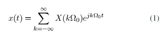
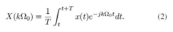
where Ω0 = 2π/T is called fundamental angular frequency and X(kΩ0) is the Fourier coefficient at the kth harmonic which is determined by
This implies that a nonsinusoidal periodical signal can be separated into a series of sinusoidal components with frequencies, which are integer multiples of the fundamental frequency. It is noted that, for the Fourier series, both the time- and frequency- domain signals have infinite length.
In order to implement Fourier analysis in computer, the signal in both time and frequency domains is discrete and has finite length. Discrete Fourier transform (DFT) is then introduced. Assume that x(t) is sampled with a rate of N points per cycle, i.e., Ts = T/N . The corresponding DFT will be
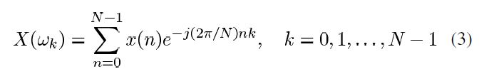
where ωk = (2π/TsN)k = (2π/T)k, X(ωk) is the so-called spectrum of x(n). Here x(n) is assumed to be one cycle of a periodical signal. In other words, the signal is supposed to precisely repeat itself for every N point. The angular frequency resolution of the spectrum is determined by the length of the signal as

Thus, if T is selected as one period of x(n), the outcome spectrum will only show components that are integer multiples of the fundamental frequency, which are defined as harmonics. However, if the data length is selected as p1 cycles (p1 > 1 and is an integer) of the fundamental, the frequency resolution will change as

This implies that once we use more than one fundamental cycle to perform DFT. It also becomes possible to obtain components at frequencies that are not integer multiples of the fundamental. These noninteger order components, according to the IEC definition, are called interharmonics.
For example, if we select five 60-Hz cycles for Fourier transform, the frequency resolution will be Δf = 60/5 = 12 Hz, then it will be possible to get bins at frequencies of 12 Hz, 24 Hz, 36 Hz …. These components, whatever the cause is, are defined as interharmonics.
There are various causes that could lead to the previously defined interharmonic components. One example is a signal that actually contains in the frequency domain a component whose frequency is noninteger multiples of the fundamental frequency. If the sampling window is selected properly so that there are exactly integer cycles of that component in the window, one can observe it at the right frequency. These are genuine interharmonics. For example, if a signal that consists of two frequencies is given by x(t) = sin(2π*60t) + 0.5sin(2π*90t), the 90 Hz component lies between the fundamental frequency and the 2nd harmonic and is a genuine interharmonic. The signal will repeat itself every two 60 Hz cycles (i.e., 33.4 ms). Therefore, if we perform DFT on this signal with a window size of 33.4 ms, the aforementioned assumption for DFT, the windowed waveform repeating itself, can be satisfied. The frequency resolution will be 60/2 = 30 Hz; consequently, one can find the 60 Hz component at the 3rd bin and the 90 Hz at the 4th bin, as shown in Fig. 1(a). This is the case of genuine interharmonics. The spectrum represents the actual signal components.

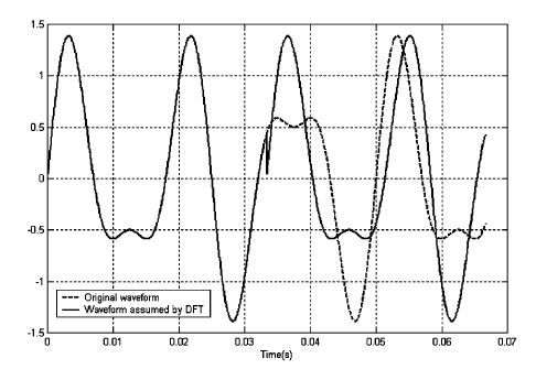
There are cases, however, where the interharmonic components are produced by the picket-fence effect of the DFT, due to sampling the signal spectral leakage. For instance, if the frequency of the noninteger harmonic component is changed to 100 Hz in last example and the selected rectangular window size is still 33.4 ms, the window will contain 3.33 cycles of the 100 Hz component. Since DFT assumes the windowed waveform will repeat itself outside the window, the repetition of the 100 Hz component is therefore incomplete. The waveform “seen” by the DFT is different from the actual waveform, as shown in Fig. 2. This leads to the creation of a main interharmonic component at 90 Hz with a low amplitude but similar to that of the genuine interharmonic at 100 Hz, and further additional spectral components as evidenced in Fig. 1(b) being not genuine due to the spectral leakage effect. Of course, the entity of these nongenuine interharmonic components strictly depends on the spectral characteristics of the window adopted (for instance, Hanning) to weight the signals and, thus, an opportune choice can reduce the spectral leakage effects (see Section III for more details).
B. Genuine Interharmonic Sources
There are some types of loads that indeed introduce interharmonics. This section will list some examples and discuss the relationship between interharmonic frequencies and load characteristics.
1) Double Conversion Systems: In general, power electronic equipment that connects two ac systems with different frequencies through a dc link can be an interharmonic source. Variable speed drives, HVDC, and other static frequency converters are typical examples of this class of sources. Their common features are that they contain an ac/dc rectifier and a dc/ac inverter, the rectifier and inverter are coupled through a reactor or a capacitor called dc link. If the reactor or the capacitor has infinite value, there will be no ripples on the dc side, and consequently the ideal rectifier will only generate characteristic harmonics of
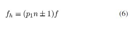
where p1 is the pulse number of the rectifier, n is an integer, and f is the power frequency.
In practical cases, however, the dc-side has finite reactor or capacitor values and, consequently, ripples at dc side are inevitable. When a rectifier’s dc link current is not ideally flat, its ac side will be modulated by the dc ripple and interharmonics could be produced. For example, for a 6-pulse rectifier, its characteristic frequencies are 60Hz, 300 Hz, 420 Hz, 660 Hz, 780 Hz…. If its dc side has a ripple of , the ac side current will be modulated as 60 ± 177 Hz, 300 ± 177 Hz, 420 ± 177 Hz, 660 ± 177 Hz….
These are interharmonic components.
For general cases, the dc-side ripple frequency can contain a series of components determined by the inverter type: current (CSI) or voltage (VSI) source inverters [3]. In CSI converters, the dc side ripple frequency depends on the pulse number, the control method, and the inverter output frequency. If the pulse number of the inverter p2 is and the output frequency is f0, the dc ripple will contain frequencies of

where is n an integer number.
TABLE I
VALUES OF PARAMETERS j AND r FOR DIFFERENT m CHOICES

In VSI converters, more complex formulas are needed to determine the dc ripple generated by the inverter. In the case of synchronous PWM modulation strategy, the harmonic frequencies generated by the inverter are evaluated as
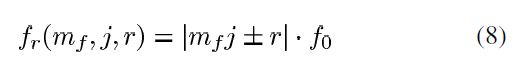
with j and r are integers depending on the modulation ratio, mf, as reported in Table I. The dependency of mf is related to the switching strategy adopted.
In both cases of CSI and VSI converters, the frequencies generated by inverters, as indicates in (7) and (8), will modulate with the rectifier’s characteristic harmonics of (6) and generate the supply-side frequencies of
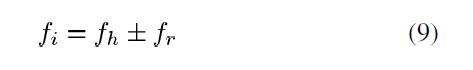
that are interharmonics of f as long fr as is asynchronous with f.
In Fig. 3, the current interharmonics absorbed by a CSI drive adopting a load commutated inverter (LCI) for f = 50 Hz and f0 = 40 Hz are reported. In Fig. 4, the current interharmonics absorbed by a VSI drive operated with synchronous PWM modulation for f = 50 Hz, mf = 9 and f0 = 40 Hz are reported. 2) Cycloconverters: The current spectral components introduced by cycloconverter are a particular case of those of other double stage converter systems and are thoroughly documented in [4] as
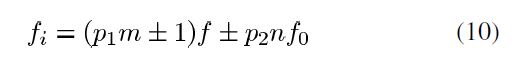
where
p1 pulse number of the rectifier section;
p2 pulse number of the output section;
mf integers;
f power frequency;
f0 output frequency of the cycloconverter.

in percentage of 230A versus interharmonic frequency

For n = 0 and m = 0, 1, 2,…, values of fi are all harmonics of f, generated by the dc component of the rectifier modulation. For n ≠ 0, m = 0, 1, 2,… and p2nf0 = kf , with k being an integer, the fi values are all harmonics of f, generated by the double modulation operated by the output section and rectifier section at the output frequency of f0. For n ≠ 0, m = 0, 1, 2,… and p2nfo ≠ kf, with k being an integer, the fi values are all noninteger multiples of , which are interharmonics and are generated by the double modulation operated by the output section and rectifier section on the output frequency, f0.
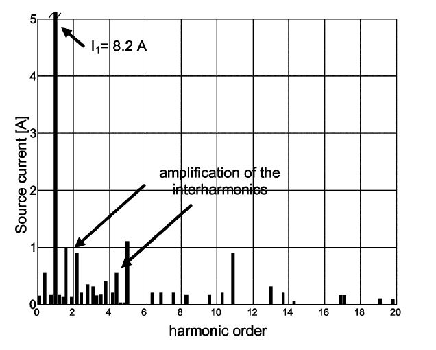
Intuitively, it is not difficult to understand the interharmonic injections by a cycloconverter, since it directly connects two systems at different frequencies. In Fig. 5, the source current spectrum absorbed by a cycloconverter working at 5 Hz in the presence of passive filters is reported [5].
3) Time-Varying Loads: Another major group of interharmonic sources are the time-varying loads, including both regularly and irregularly fluctuating loads.
Typical examples of regularly fluctuating loads, which cause sinusoidal and square modulated signals, are welder machines, laser printers, and devices with integral cycle control. For such loads, the frequency at which the load varies will determine the frequencies of interharmonics. Assuming the system voltage is v(t) = sin2πft and a load has a characteristic of R(t) = 1-rsin2πf0t, where r < 1 and f0 is the load varying frequency, then the load current is
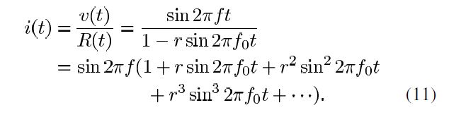
Further mathematical operation on (11) can show i(t) that contains interharmonic components of f ± f0, f ± 2f0, f ± 3f0, …, etc. As a result, interharmonics will be seen in the current spectrum as long as is asynchronous with . In more realistic situations, the load is modulated by means of square wave modulating functions and consequently the spectrum is richer in interharmonic components. In Fig. 6 an example of current absorbed by a laser printer is reported [6].

Typical examples of irregularly fluctuating loads are arc furnaces. The time-varying and nonlinear behavior of the arc generates in both current spectra with several spectral components, including harmonics and interharmonics, which are difficult to model analytically.
In the case of ac arc furnaces, significant interharmonics are concentrated around the power system frequency. The dc arc furnaces can be characterized by a significant presence of interharmonics around the harmonics of the ac/dc converters. In practice, the ac side of the ac/dc converter is modulated by the dc ripple which depends on the dc arc behavior and on the ac/dc converter control system. Since the arc behavior is “chaotic,” the interharmonics generated by arc furnaces are characterized by constantly changing chaotic frequencies.
.
Finally, with reference to a window in which the frequency variation can be neglected (see also Section III), the current spectra of an ac and a dc arc furnace are shown in Fig. 7.

4) Wind Turbines: Regarding power generation, wind turbines may play an important role for producing voltage interharmonics. In this case, the origin of interharmonics is essentially mechanical. In particular, during the continuous operation of the fixed-speed wind turbines, wind variations and the tower shadow effect result in power fluctuations and, hence, in line voltage interharmonics. Fig. 8 reports the mechanical torque, M, from the wind turbine (solid line) and the electrical torque, Me, (dotted line) from a wind generator obtained in [7]. Fig. 9 reports, in logarithmic axes, the output voltage spectrum which results rich of interharmonics around the fundamental frequency as a consequence of the mechanical torque oscillations shown Fig. 8. The results are obtained from both the time-domain model (solid line) and the frequency-domain model (circled line) described in [7].


5) Unexpected Sources: A nonlinear load or network component by itself is not able to generate interharmonics. For instance, a simple rectifier or reactive power static generators when it reacts to the interharmonic components present in the supply voltage, only absorbing interharmonic currents. Some interharmonic current components are at the same frequencies of the voltage and some are at frequencies determined by the modulation operated by the nonlinear load on the original voltage interharmonic frequencies. Therefore, these components become sources of new interharmonic frequencies when interharmonic supply voltages are present. Simple case studies have demonstrated high sensitivity (more than two times of the 50 Hz value) at specific frequency couples (voltage and current) corresponding in the example of Fig. 10, reported in [8], to intersections (20 Hz, 20 Hz), (20 Hz, 120 Hz), (120 Hz, 20 Hz), (120 Hz, 120 Hz). It means that the 20 Hz (or the 120 Hz) voltage interharmonic produces high current interharmonics both at 20 and 120 Hz.

III. INTERHARMONICS ASSESSMENT
A practical assessment of interharmonics involves various aspects and presents some difficulties. One of the main difficulties is due to spectral leakage phenomenon and picket-fence effect of the DFT already mentioned in Section II-A. Therefore, techniques for the interharmonics assessment [9] are of primary interest and it is useful to develop some basic considerations.
An ideal technique should ensure that all nonzero bins refer to genuine interharmonics or harmonics: this means obtaining conditions in which the sampling window is effectively synchronized with all the signal frequency components.
When the frequencies of genuine interharmonics present in the signal are known a priori, it is possible to introduce the Fourier fundamental frequency, fF, as the greatest common divisor of all the frequency components contained in the signal. Then, the signal is sampled with windows of duration being an integer multiple of the corresponding Fourier fundamental period, Tf = fF. In practical cases, it may happen that fF reaches a very small value with corresponding enormous Tf. A simple example can help to understand the aforementioned difficulties and to introduce some practical solutions adopted: a signal composed by two tones, one harmonic, at 50.00 Hz, and the other interharmonic, at 34.50 Hz, is considered, as shown in Fig. 11(a).

The Fourier fundamental frequency is, of course, equal to 0.50 Hz [Fig. 11(b)] and the interharmonic appears as the 69th harmonic of it. The corresponding fundamental period is of 2 s so, assuming a sampling frequency of 5 kHz, needed to manage frequency components until 2.5 kHz, the enormous value of 10000 samples should be processed. Moreover, during such a long period of time, in real systems, the signal components (harmonic and interharmonic) may vary their amplitudes, frequencies and phase angles.
Reducing the frequency resolution to 1 Hz [Fig. 11(c)], four main spectral lines at 33 Hz, 34 Hz, 35 Hz and 36 Hz (black lines) appear in the spectrum instead of the original component
(gray line). In spite of a still high computational burden (TF = 1 s) , the energy of the original interharmonic component is spilled in different bins and the information about the exact interharmonic amplitude, frequency and phase angle is lost (or difficult to obtain).
The IEC Standard 61000-4-7 [10] and the under-revised IEEE 519 fix the frequency resolution of the spectral analysis at 5 Hz as a trade-off between accuracy and computational burden reduction. The effects on the signal of Fig. 11(a) are reported in Fig. 11(d) and are similar to those illustrated in Fig. 11(c); they are managed with the grouping technique described in the following part of this section.
Comparing Fig. 9, it is possible to observe as the frequency resolution adopted affects the representation of the actual interharmonic component.
Other important signal processing aspects are reported in the standards that suggest:
1) DFT performed over a rectangular time window of exactly ten cycles for 50 Hz systems or exactly twelve cycles for 60 Hz systems, which is approximately 200 ms in either case;
2) phase-locked loop or other line frequency synchronization techniques to reduce the errors due to the spectral leakage effects due to the desynchronization of fundamental and harmonics [9].
Furthermore, the remarkable concept of harmonic and interharmonic groups and subgroups is introduced. In particular, the subgrouping concept is illustrated in Fig. 12 with reference to the 7th, 7.5th and 8th order subgroups. The amplitude, Cn+0.5-200-ms, of the interharmonic subgroup of order n + 0.5 is defined as the root mean square (rms) value of all the interharmonic components between adjacent harmonic subgroups.

The standard approach is attractive for compliance with monitoring and compatibility testing, since compatibility levels can be fixed on the basis of the energy of the specified interharmonic groups or subgroups rather than relying on the measurement of specific tones. It is also possible to improve its accuracy by means of Hanning windowing as illustrated in [3] of [11].
Regarding high-resolution methods, recently in [11] different proposals of both DFT-based and Prony-based advanced methods have been recalled and compared to each other; both
approaches succeed in estimating the exact interharmonic frequency. These techniques, together with time-frequency techniques [12], are of crucial importance for accurate analysis when time-varying or chaotic signals appear in the system.
IV. MODELING INTERHARMONIC SOURCES
The interharmonic currents generated by nonlinear devices are more affected by the waveforms and peak values of supply voltages and by the supplied load operating point than harmonic currents. Further on the current magnitude and phase angle, this aspect regards also the current frequency. Therefore, it is desirable to represent the devices with their actual nonlinear v – i characteristics in distortion studies, instead of as voltage independent harmonic current sources. Depending on the source characteristics, comprehensive models for interharmonic sources are summarized as follows.
• Low-power analogue electronic simulators consisting of a number of scale model converters and model power system components, such as high Q-factor chokes, low magnetizing current transformers, capacitors, and small 6-pulsethyristor bridges.
• Time-domain models that can refer in principle to very general schemes, taking into account any kind of nonideal conditions as background distortion, unbalances, magnetic material saturation, and firing asymmetries.
• Frequency-domain models based on the modulation theory extended for double stage converters, which constitute very fast to solve models, flexible and characterized by accuracy determined by the accuracy of the modulation functions utilized.
• A hybrid of previously described models. In the following for the different kinds of sources referred to Section II-B, specific information on the different models proposed in the relevant literature is reported.
A. Double-Stage Converters
A great effort has been made in modeling HVDC links and high-power adjustable speed drives based on line-commutated converters [2], [13]–[18]. An important aspect of the problem is related to the modeling of ac/dc/ac conversion systems in order to achieve a detailed description and computational efficiency. Various models are available to obtain the ac and the dc absorbed currents: experimental analog, time- and frequency- domain models [15]. Each of them is characterized by different degrees of complexity in representing the converters, the dc link, and the ac supply systems. In most cases, frequency-domain models operate with different degrees of complexity by using the modulation function approach and do not require heavy computational efforts and are very quick in execution [13]–[21].
On the other hand, less attention has been devoted to different systems such as ASD using PWM inverters. This is partly due to the assumption that the dc capacitor completely eliminates the interaction between the two converters [22], [23]. In other words, the generation of interharmonics for an HVDC and the high-power ASD has been modeled and analyzed in depth [24], while the interharmonics produced by PWM ASD are considered negligible [23], whichever is the drive power or the operating point for a given drive. However, a more detailed analysis for PWM ASD has been recently developed in [25].
B. Cycloconverters
In [26], an electromagnetic transient simulation program with a graphical interface of a cycloconverter including a detailed three-phase transformer model with nonlinear magnetizing characteristic was presented. In [27], a three-phase bridge cycloconverter for a traction load is modeled. The simulation results from an ideal model (i.e., no losses, no resistance in the thyristors, no inductance in the load, and ideal current source load) are compared with Pspice simulation results and actual measurements. The Pspice model contains high-order models for the thyristors and an RL load model with load dynamics.
C. Time-Varying Loads
Regarding regularly fluctuating loads, in [28], the impact of switching strategies on PQ for integral cycle controllers is considered. The load current is evaluated as a time-domain product of a modulating signal and a 60 Hz sine wave. The modulating signal is taken as the addition of a series of phase shifted square functions, representing the integer number of cycles “on” and the integer number of cycles “off” that constitute the period of the resulting modulated wave. The 60 Hz current is that obtained for ac circuit in the steady-state conditions in a continuous duty. For irregularly fluctuating loads, as described in [29], several models have been proposed in the relevant literature for ac arc furnace modeling. In the next the models that appear most suitable for interharmonic assessment are considered.
In [30] ac arc furnaces are represented by voltage generators. The simulation of arc operation is realized by varying the amplitude of the voltage generator that can provide, besides the fundamental voltage, harmonics, as well as interharmonics produced by the arc. In [31] and [32] the electric ac arc is simulated by a proper resistance used to describe both the nonlinear voltage-current characteristic of the arc and its changes with time. The choice of the time-varying nonlinear resistance is effective in order to produce voltage distortions and fluctuations at frequencies and typical levels of actual ac arc furnaces. In [33] a voltage-current characteristic based on Mayr’s model is proposed. This arc model incorporates the most significant aspects of the physical mechanisms of the arc. In [34] and [35] power or energy balance models are used to represent the arc in time or frequency domain while in [36] a hybrid model, based on fictitious diodes and dc voltage sources, is used for inclusion in a harmonic power flow.
Further ac arc models proposed in the literature are based on stochastic or adaptive models [31], [37]–[40] which employ a band-limited white noise generator to simulate arc
length/resistance, a voltage source model, and a resistance model. DC arc models are proposed in [41] and [42] where the typical voltage-current characteristic tuning requires significant analyses of on-site measurements. Another example of dc arc furnace model is reported in [43] where the dc arc is modeled as a resistance randomly varying at periodical manner. Recently, the electrical fluctuations in the arc furnace voltage have been proven to be chaotic in nature, hence some chaos-based models have been applied to simulate ac and dc arc furnaces [44]–[47].
D. Wind Turbines
As is well known, the oscillatory components of the mechanical torque in wind turbines produce the voltages interharmonic components that can cause the Light Flicker. These oscillations have stochastic as well as deterministic origin because they are produced mainly by wind variations and the tower shadow effect. Comprehensive modeling is needed requiring modeling of wind input, that includes both stochastic and deterministic effects, and mechanical elements further on the electrical elements. General modeling aspects of wind turbines are reported in [48]. References [49] and [50] also predict the flicker level and interharmonics produced by a wind turbine when connected to the power grid and various generator models in time domain are used. In [7], a fast and accurate method in the frequency domain is proposed and a comparison of the results obtained by different approaches, as shown in Fig. 9 of Section II, is reported.
E. Unexpected Sources
In [51], the couplings among interharmonic supply voltages and absorbed currents are modeled by means of so-called “frequency coupling matrices” obtained with a circular convolution method, starting from the converter switching functions. The absolute values of the matrix elements in positions (i , j) measure the sensitivity of the th current component to the jth supplying voltage component, assuming that the operating point of the system is not modified.
The result reported highlights that conversion systems exhibit greater frequency coupling at interharmonic frequencies than at harmonic frequencies. Therefore, modeling of traditional nonlinear loads cannot miss interharmonic consideration.
V. EXTENDING POWER SYSTEM HARMONIC ANALYSIS
According to the assessment procedures introduced in Section IV, the introduction of a base frequency of the frequency- domain analysis allows transforming the problem of modeling harmonics and interharmonics of the system frequency (50 or 60 Hz) into that of modeling harmonics of the base frequency (i.e., 5 Hz). This allows, in principle, to adopt each kind of technique proposed for harmonic penetration studies, also in the presence of interharmonics. This section describes the problems difficulties and cares to be adopted in the presence of interharmonics.
Nodal harmonic and interharmonic voltages are the result of harmonic and interharmonic current injection in nodes and propagation through the network. The current injection depends itself on the voltage supply. For the harmonic and interharmonic distortion analysis in electrical power systems, it is recommended that the methods adopted to evaluate the current injection are as comprehensive as possible, because they have to be able to model nonideal conditions such as ac-side imperfections (supply voltage distortion and unbalance, supply system impedance unbalance, transformer magnetic saturation, etc.). Simplified methods, that do not take into account the nonideal conditions, may lead to erroneous numerical results for the actual behavior of the system.
To include interharmonics in distortion models means to start from the critical analysis of classical models for harmonics to extend such models when possible [52]. Particular attention must be devoted to the problems of the frequency resolution and of the computational burden. As for components such as cables, overhead lines, and capacitors banks, specific models are not required. Those models developed for harmonic studies can be easily applied.
As for electromechanical components, in particular, transformers and induction motors, are characterized by the need of specific models for interharmonics, mainly for subharmonics, which have to be still developed. Basic results are reported in [29] and [53]. It seems that their modeling will require the use of accurate time-domain approaches.
A. Classical Methods for Harmonic Analysis
The methods referred to in the relevant literature for harmonic penetration studies can be classified as
a) direct current injection;
b) harmonic power flow;
c) iterative harmonic analysis;
d) experimental analog modeling of the whole system;
e) time-domain modeling of the whole system.
The first three methods have the common characteristic of representing and solving the ac system equations in the frequency domain. Models b) and c) are both iterative and, in particular, model b) uses a Newton–Raphson algorithm while model c) uses a Gauss–Seidel algorithm. A combination of both types of algorithms have also been proposed. The direct injection method is able to take into account unbalances but not interactions between converters. The harmonic power flow is able to take into account the interaction between converters, and in its most recent formulation, which takes into account unbalances and other nonideal conditions. The iterative harmonic analysis is able to take into account both the unbalance and the interaction between converters and also other nonideal conditions. Convergence problems may arise for methods b) and c); solutions to such problems have been proposed, as described in [52], for both models.
The remaining two models, d) and e), analyze each system component or subsystem by means of equivalent circuits in the time domain. The low-power analogue models or time-domain models may obtain in principle any desired level of details. Practical difficulties limit the use of the first of these methods to the case of a small system size, while references to the second category with new approaches seem to offer interesting perspectives [29].
B. Extension to Include Interharmonics
In principle, it is very easy to include interharmonics in the classical model by the main concept of the Fourier fundamental periods, developed in Section IV. At the end of the analyses on the voltage e(t), it is very easy to recognize as harmonics the signal components, whose frequencies are integer multiples of the system fundamental frequency, and as interharmonics as the other components.
In practice, the following considerations apply [52].
• the extension of low-power analog models and of time-domain models does not suffer from specific problems but practical difficulties limit the use of these models to cases of small system size as is typical also for the case of conventional harmonic analysis;
• the extension of the direct injection method is easy to obtain but gives, as typical for this kind of method, inaccurate results;
• the extension of the harmonic power flow seems possible but very difficult as a consequence of the difficulties which arise in modeling nonlinear loads in the frequency domain when interharmonics are present;
• the extension of the iterative harmonic analysis is complex if one wants to use analytical expressions to model the nonlinear loads while, if time-domain simulations are used, only computational effort problems remain and this method can be utilized, obtaining high accuracy results. Some more details about the extension of the methods are reported in the Appendix.
C. Computational Burden
Extending all classical models to include interharmonics implies taking into account a larger number of frequency components and referring to a larger waveform periodicity interval.
Let us consider the case in which a fixed resolution frequency ff is introduced (see Section III). Both harmonic and interharmonic frequencies are integer multiples of the resolution frequency. Therefore, all of the components can be treated as harmonics of ff. Give a maximum frequency of interest, fmax and the number of components of interest, Nihmax, which is equal to the ratio between fmax and ff. Compared with the maximum number of components when only harmonics are present, it is easy to demonstrate that it is equal to amplified by the factor of f / ff , where is the system fundamental frequency. For instance, if fmax = 2500 Hz, ff = 5 Hz, and f = 50 Hz, it means that = 500 while = 50.
Similar considerations apply to the periodicity interval, which is of great importance for time-domain simulations. It also results in amplification by the same factor of f / ff . With the same conditions as the previous example, the minimum time interval to be simulated in the presence of interharmonics, once reaching steady-state conditions, is equal to 200 ms instead of 20 ms. Comparisons among different models in the presence of interharmonics give the same results that are well known for the same models in the absence of interharmonics.
VI. CASE STUDIES
Two case studies referred to two popular schemes of adjustable speed drives (ASDs) are reported in this section. Methodologies previously described are used to obtain the results reported.
A. LCI ASD
Several numerical experiments are reported in [54] to test some of the methods described in Section V-B. The results obtained by the well-known EMTP are utilized as a reference to verify the accuracy obtained by a direct method and by an iterative method.
The results obtained for the LCI drive for asynchronous motors, as depicted in Fig. 13, are reported.
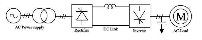
TABLE II
PARAMETERS FOR THE LCI ASD

The system parameters are listed in Table II. The system was simulated for output frequency values varying from 17.5 to 50 Hz with a resolution of 0.5 Hz [54]–[56].
TABLE III
CURRENTS FOR ASD-A OF TABLE II WITH FM = 47.5 Hz
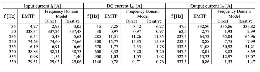
Table III reports the currents for an output frequency of 47.5 Hz with αR = 41.4° and αI = 120.2° . The inverter output current is also reported due to the great interest recently devoted to the negative effects of interharmonics, mainly at low frequency, in terms of the reduction of asynchronous motor expected life [57]. The errors of both frequency-domain models are acceptable and the highest values appear at specified interharmonic frequencies and in correspondence of low-amplitude values. The iterative analysis effects, in terms of accuracy, are always present but never relevant as a consequence of the noncriticality of the operating point considered.
TABLE IV
CURRENTS FOR ADS-A OF TABLE II WITH fo = 47.5 Hz
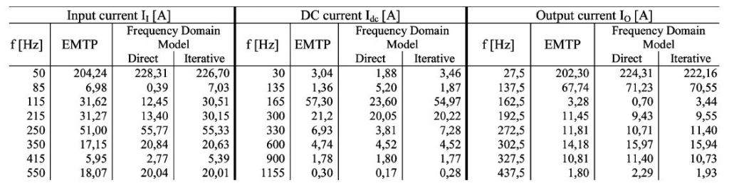
Table IV reports the currents for the output frequency of 27.5 Hz, with αR = 66.6° and αI = 122.7°. The errors are not acceptable for the direct method at least for all interharmonic components. This is due to the value of the output frequency, which causes strong interactions between the converter and the output impedance. The iterative analysis succeeds in improving the accuracy and makes the errors acceptable. Moreover, in [54] it is shown that interharmonic components are evaluated with relevant errors by direct method in a wide range of motor frequencies (from about 21 to 37.5 Hz); the iterative analysis always solves the problem.
TABLE V
SIMULATION AND LABORATORY TEST CONDITIONS

B. PWM ASD
In [58], analytical solutions of harmonic/interharmonic characteristics of the VSI-fed ASD shown in Fig. 14 are compared with time-domain simulation results obtained by the use of Simulink. Laboratory tests for validation of the solutions are also conducted: the test setup, which consists of the ideal three-phase ac source, a VSI-fed ASD, an induction motor, an electrodynamometer module, and a LabView-based data-acquisition/monitoring computer system and the experimental conditions considered are fully described in [58]. Table V reports simulations and laboratory test conditions.

In Figs. 15 and 16, the results that are indicated are the harmonic and interharmonic spectra of the ASD input current with respect to the motor operating frequency of 40 Hz. It is possible to observe that the solutions obtained by the approach proposed in [58] are in good agreement with those obtained by using the time-domain simulation tool and by laboratory tests.

frequency of 40 Hz at a full-load power level.
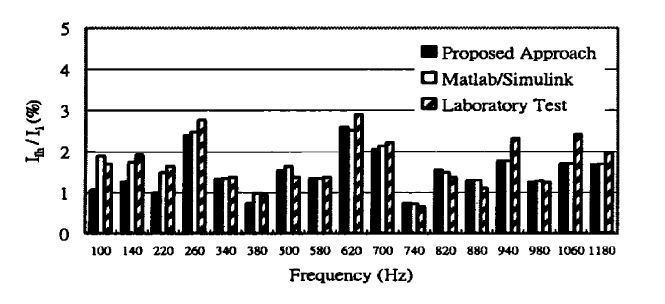
operating frequency of 40 Hz at a full-load power level.
C. Computational Burden
As recalled in Sections III and V-C, the computational burden of numerical simulations in the presence of interharmonics is strongly influenced by the choice of the frequency resolution to be adopted. Moreover, the choice of the specific modeling technique to use plays an important role.
TABLE VI
LCI DRIVES: EXECUTION TIMES AND SPEED-UP VERSUS ff VALUES
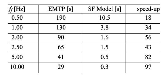
TABLE VII
PWM DRIVES: EXECUTION TIMES AND SPEED–UP VERSUS ff VALUES
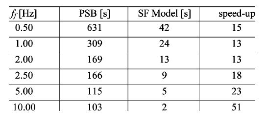
Tables VI and VII report the results in terms of execution times and “speedup” with reference to two case studies (an LCI drive and a PWM inverter drive) reported in [56], for different values of the frequency resolution ff . The solution methods considered are:
• time-domain simulations [Electromagnetic Transient Program (EMTP) and power system blockset (PSB)]
• Models based on switching function approach [55], SF Model, that combine models described in Section IV-A for ASD and the iterative method principle described in Section VIII-B.
Reference is made to a 1.7 GHz PC. The times reported in both tables do not take into account the final DFT application to time-domain waveforms and the speedup is defined as the ratio between time-domain and SF models simulation times. It is worthwhile underlining that time-domain simulations suffer from the need of waiting for the end of the unavoidable transient stage affecting the beginning of the simulation [56].
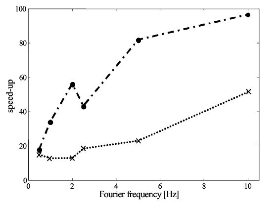
Looking at Tables VI and VII, it is evident that:
- whichever is the model, execution times sensibly increase as ff decreases;
- SF models are always sensibly faster than time-domain modeling;
- the speedup reaches very high values and varies with ff .
Finally, Fig. 17 shows that the reduction of the calculation time when the Fourier fundamental frequency increases is more sensible for the models than for the time-domain simulator, which seems to be due to the absence of transient stages in the models.
VII. CONCLUSIONS
Some of the most remarkable issues related to interharmonic theory and modeling have been presented. Starting from the basic definitions and concepts, attention has been firstly devoted to interharmonic sources. Then, the interharmonic assessment has been considered with particular attention to the problem of the frequency resolution and of the computational burden associated with the analysis of periodic steady-state waveforms. Finally, modeling of different kind of interharmonic sources and the extension of the classical models developed for power system harmonic analysis to include interharmonics have been discussed. Numerical results for the issues presented have been given with referring to case studies constituted by popular schemes of adjustable speed drives.
APPENDIX
A) Direct Current Injection: The direct injection method is the simplest method because the evaluation of current harmonics for each load is independent from the evaluation of the ac system voltage harmonics. The method, in its typical form, is based on the following steps.
Step 1) The execution of a conventional load-flow study to obtain all bus voltages with assuming converter busses are load buses.
Step 2) An estimation of the converter currents at each harmonic using bus voltages from step 1) by means of time-domain simulations, analytical models, or experimental measurements.
Step 3) The calculation of the bus admittance matrix, Yh, at each frequency of interest.
Step 4) The use of expression, Ih = YhVh, to calculate the vector of voltage harmonics, Vh, ∀h.
In order to take into account the presence of interharmonics, the following additional factors are necessary.
a) To foresee all the interharmonic frequencies, fi, that will be present in the frequency range of interest.
b) During Step 2) to estimate the synchronous motor drive currents at each harmonic and interharmonic frequencies by means of an appropriate frequency-domain experimental analogue or a time-domain model as discussed in [1] of [52] or by analyzing available field measurements.
c) During Step 3) for each interharmonic frequency, fi, of interests to calculate the corresponding bus admittance matrix, Yi, starting from the ac system knowledge or, if this is not possible, by interpolation of the known harmonic admittance matrix values.
d) During Step 4), the evaluation of the vector of voltage interharmonics Vi using the expression Ii = YiVi for each interharmonic frequency, fi, of interests.
It is important to note that it is not necessary to modify the converter model adopted in step 2), because this method does not account for supply harmonic and interharmonic distortion in modeling the converters.
In conclusion, no particular difficulties arise in extending the direct injection method to take into account interharmonics. The direct injection method presents the well-known advantages of speed, extendibility to unbalanced cases and the absence of divergence phenomena. Disadvantages are the poor accuracy and the impossibility of taking into account interaction between converters.
B) Iterative Harmonic Analysis: The iterative harmonic analysis is a method based on a Gauss–Seidel algorithm. It can be summarized by the following fundamental steps.
Step 1) Input information is obtained on system component characteristics and ac system impedances. Then, initial conditions are evaluated by means of an ac/dc three-phase power-flow for each node supplying a converter.
Step 2) Starting from the voltage waveforms at the converter terminals, the current waveform i(t) over one cycle under steady-state conditions is estimated for each converter.
Step 3) The steady-state time-domain current waveforms previously obtained for each converter are subject to a FFT in order to obtain the vector, Ih, of their harmonic current components.
Step 4) The current harmonics Ih, obtained in 3) are utilized to perform steady-state harmonic analyses of the ac system by means of the harmonic impedances of the ac system to obtain the corresponding updated vector, Vh, of voltage harmonics at the converter busses.
Steps 2)–4) are repeated until convergence is achieved. That is, until the voltage harmonics do not change significantly compared to those obtained in the previous iteration.
In greater detail, Step 2) requires for each converter the solution of analytical models proposed in [12]–[24] of [52] or, as an alternative, a time-domain simulation in [5], [16], and [25] of [52]. In a recent version proposed in [14] of [52], the algorithm described has been modified to include in the iteration process the three-phase load-flow stage to take into account the fundamental power variations produced by the converters.
Extension: In order to take into account also the presence of the interharmonics, the following additional factors are necessary.
a) To foresee all the interharmonic frequencies, fi, that will be present in the frequency range of interest.
b) To calculate for each interharmonic frequency, fi, of interest the corresponding bus admittance matrix Yi.
c) To substitute Step 2) by Steps 2)’ for conventional converters and 2)” for the synchronous motor drive.
d) To start Step 2)’ from the voltage waveforms at the conventional converter terminals and estimates the current waveforms i(t) over an appropriate number of system fundamental frequency cycles to obtain an entire Fourier’s fundamental frequency cycle under steady-state conditions for each converter.
e) Step 2)” starts from the voltage waveform at the synchronous motor drive terminals and estimates the current waveforms over an entire Fourier’s fundamental frequency cycle under steady-state conditions for each synchronous motor drive.
f) During the Step 4), to add the evaluation of the vector voltage interharmonics Vi using the expression, Ii = YiVi, for each interharmonic of interest.
It is worthwhile underlining that the foreseen of all the interharmonic frequencies present in the frequency range of interest is necessary to fix the frequency to be used in the ac analysis part. This can be done by means of theoretical studies, such as those reported in [3], or, in absence of enough information on the system under study, choosing a fixed frequency cycle based on engineering considerations (see also Section III).
In 2)’ analytical models can be, in principle, utilized extending the current waveforms construction proposed in [12] of [52] to the entire Fourier’s fundamental cycle. Such solution seems suitable but, to the author knowledge, it has not been experimented. In step 2)” new synchronous motor drive analytical models should be utilized. To the authors’ knowledge, they are not yet available and seem to be difficult to obtain. To perform some first experiments, about the iterative harmonic analysis model extension, it is possible to adopt time-domain simulations for both 2)’ and 2)” steps, sacrificing the computational method efficiency.
In conclusion, some difficulties arise in extending the iterative harmonic analysis model to take into account also interharmonic distortion, particularly the use of the time-domain model for solving the nonlinear loads at each iteration. The iterative harmonic analysis model presents the well-known advantages of comprehensive modeling, which accounts for distortion and unbalance, impedance resonances, interaction between converters and other non ideal conditions. It presents the disadvantages of convergence problems that can be overcome by means of appropriate techniques (please see [5], [15]–[17] of [52]).
C) Multifrequency Power Flow: The three main constituent parts of a multifrequency power flow are
1) a three-phase ac/dc power flow at the fundamental frequency [59];
2) a three-phase harmonic flow model of the linear part of the power system with multiended harmonic sources [4].
3) a harmonic domain representation of the individual nonlinear components [60].
These three components need to be solved simultaneously using the Newton method. The full Jacobian matrix, with no decoupling to reduce the number of converter mismatch equation evaluations by reducing the number of iterations to convergence, is utilized. A unified power flow and harmonic solution in Cartesian coordinates is more efficient than the one in polar coordinates.
Extension: In order to solve for interharmonic frequencies, the base frequency of the harmonic domain is reduced to the highest common denominator of the frequencies of all the harmonic and interharmonic frequencies.
Interharmonics can be accommodated efficiently by means of an adaptive technique complemented by interpolation between integer frequencies [61]. A large proportion of the harmonics and interharmonics are below a certain threshold. Thus, by solving only for the significant frequencies the solution time can be substantially reduced.
To avoid updating the Jacobian at every iteration, during the first two iterations, the current and voltages frequency components produced by the converters from their distorted inputs are combined at their respective busses. These combined contributions are then limited with a tolerance level, and sparse lists are formed. These lists are used to form the solution variables, mismatch arrays, and a Jacobian to update only the selected frequencies. It is found that after two of such iterations, all of the significant frequencies have been selected and that the solution arrays can then be held constant for the remainder of the solution. From then on, the Jacobian is only recalculated and redecomposed, if the rate of convergence drops below a specified level.
The computational burden of the converter model is reduced by using basic modulation theory to the six-pulse converter, to predict what frequencies are going to be generated from the terminal frequencies, and consequently only do the convolution for those frequencies.
ACKNOWLEDGMENT
The authors would like to acknowledge the following members for their major contributions: A. Testa (editor), G. Carpinelli, G. Chang (Chair, Co-editor), V. Dinavahi, R. Langella, T. Ortmeyer, and W. Xu.
REFERENCES
[1] Interharmonic in Power System IEEE Interharmonic Task Force, Cigré 36.05/CIRED2, WG2/UIEPQ/CC02 Voltage Quality Working Group [Online]. Available: http://grouper.ieee.org/groups/harmonic/iharm/docs/.
[2] R. Yacamini, “Power system harmonics. Iv. Interharmonics,” Power Eng. J., vol. 10, no. 4, pp. 185–193, Aug. 1996.
[3] F. D. Rosa, R. Langella, A. Sollazzo, and A. Testa, “On the interharmonic components generated by adjustable speed drives,” IEEE Trans. Power Del., vol. 20, no. 4, pp. 2535–2543, Oct. 2005.
[4] J. Arrillaga and N. R. Watson, Power System Harmonics, 2nd ed. New York: Wiley, 2004.
[5] D. Basic, V. S. Ramsden, and P. K. Muttik, “Performance of combined power filters in harmonic compensation of high-power cycloconverter drives,” in Proc. 7th Int. Conf. Power Electronics and Variable Speed Drives, Sep. 1998, pp. 674–679.
[6] D. Gallo, R. Langella, and A. Testa, “Desynchronized processing technique for harmonic and interharmonic analysis,” IEEE Trans. Power Del., vol. 19, no. 3, pp. 993–1001, Jul. 2004.
[7] C. Vilar, J. Usaola, and H. Amaris, “Frequency domain approach to wind turbines for flicker analysis,” IEEE Trans. Energy Convers., vol.18, no. 2, pp. 335–341, Jun. 2003.
[8] R. Carbone, A. L. Schiavo, P. Marino, and A. Testa, “Frequency coupling matrixes for multi stage conversion system analysis,” Eur. Trans. Elect. Power, vol. 12, no. 1, pp. 17–24, Jan./Feb. 2002.
[9] D. Gallo, R. Langella, and A. Testa, “Interharmonic measurement in IEC framework,” presented at the IEEE Summer Power Meeting, Chicago, IL, Jul. 2002.
[10] General Guide on Harmonics and Interharmonics Measurements, for Power Supply Systems and Equipment Connected Thereto, IEC Std. 61000-4-7, 2002.
[11] A. Bracale, G. Carpinelli, R. Langella, and A. Testa, “On some advanced methods for waveform distortion assessment in presence of interharmonics,” in Proc. IEEE Power Eng. Soc. General Meeting, Montreal, QC, Canada, Jun. 2006.
[12] A. Bracale, G. Carpinelli, Z. Leonowicz, T. Lobos, and J. Rezmer, “Measurement of IEC groups and subgroups using advanced spectrum estimation methods,” in Proc. Instrumentation and Measurement Technology Conf., Sorrento, Italy, Apr. 2006.
[13] M. B. Rifai, T. H. Ortmeyer, and W. J. McQuilan, “Evaluation of current interharmonics from AC drives,” IEEE Trans. Power Del., vol. 15, no. 3, pp. 1094–1098, Jul. 2000.
[14] L. Hu and R. E. Morrison, “The use of modulation theory to calculate the harmonic distortion in HVDC systems operating on an unbalanced supply,” IEEE Trans. Power Syst., vol. 12, no. 2, pp. 973–980, May 1997.
[15] A. R. Wood and J. Arillaga, “The frequency dependent impedance of an HVDC converter,” IEEE Trans. Power Del., vol. 10, no. 3, pp. 1635–1641, Jul. 1995.
[16] B. C. Smith, N. R. Watson, A. R. Wood, and J. Arillaga, “Harmonic tensor linearization of HVDC converters,” IEEE Trans. Power Del., vol. 13, no. 4, pp. 1244–1250, Oct. 1998.
[17] B. C. Smith, N. R. Watson, A. R. Wood, and J. Arillaga, “Steady state model of the AC/DC converter in the harmonic domain,” Proc. Inst. Elect. Eng., Gen., Transm. Distrib., vol. 142, no. 2, pp. 109–118, Mar. 1995.
[18] R. Yacamini and J. C. de Oliveira, “Harmonics in multiple converter systems: A generalised approach,” Proc. Inst. Elect. Eng., Gen., Transm. Distrib., vol. 127, no. 2, pp. 96–106, Mar. 1980.
[19] E. V. Person, “Calculation of transfer functions in grid-controlled converter systems,” Proc. Inst. Elect. Eng., vol. 117, no. 5, pp. 989–997, May 1970.
[20] Y. Jiang and A. Ekstrom, “General analysis of harmonic transfer through converters,” IEEE Trans. Power Electron., vol. 12, no. 2, pp. 287–293, Mar. 1997.
[21] P. Marino, C. Picardi, and A. Russo, “AC characteristics in AC/DC/DC conversion,” Proc. Inst. Elect. Eng., Elect. Power Appl., vol. 130, no. 3, pp. 201–206, May 1983.
[22] L. Hu and R. Yacamini, “Calculation of harmonics and interharmonics in HVDC schemes with low DC side impedance,” Proc. Inst. Elect. Eng., Gen., Transm. Distrib., vol. 140, no. 6, pp. 469–475, Nov. 1993.
[23] L. Hu and R. Yacamini, IEEE Trans. Power Electron., vol. 7, no. 3, pp. 514–525, Jul. 1992.
[24] R. Carbone, D. Menniti, R. E. Morrison, E. Delaney, and A. Testa, “Harmonic and interharmonic distortion in current source type inverter drives,” IEEE Trans. Power Del., vol. 10, no. 3, pp. 1576–1583, Jul. 1995.
[25] R. Carbone, F. D. Rosa, R. Langella, A. Sollazzo, and A. Testa, “Modelling of AC/DC/AC conversion systems with PWM inverter,” presented at the IEEE Summer Power Meeting, Chicago, IL, Jul. 2002.
[26] Z. Wang and Y. Liu, “Modeling and simulation of a cycloconverter drive system for harmonic studies,” IEEE Trans. Ind. Electron., vol. 47, no. 3, pp. 533–541, Jun. 2000.
[27] Y. Liu, G. T. Heydt, and R. F. Chu, “The power quality impact of cycloconverter control strategies,” IEEE Trans. Power Del., vol. 20, no. 2, pt. 2, pp. 1711–1718, Apr. 2005.
[28] Y. N. Chang, G. T. Heydt, and Y. Liu, “The impact of switching strategies on power quality for integral cycle controllers,” IEEE Trans. Power Del., vol. 18, no. 3, pp. 1073–1078, Jul. 2003.
[29] “Modeling devices with nonlinear voltage-current characteristics for harmonic studies,” IEEE Trans. Power Del., vol. 19, no. 4, pp. 1802–1811, Oct. 2004.
[30] M. Loggini, G. C. Montanari, L. Pitti, E. Tironi, and D. Zaninelli, “The effect of series inductors for flicker reduction in electric power systems supplying arc furnaces,” in Proc. IEEE Ind. Appl. Soc. Annual Meeting, Toronto, ON, Canada, Oct. 1993, pp. 1496–1503.
[31] G. C. Montanari, M. Loggini, A. Cavallini, L. Pitti, and D. Zaninelli, “Arc-furnace model for the study of flicker compensation in electrical networks,” IEEE Trans. Power Del., vol. 9, no. 4, pp. 2026–2036, Oct. 1994.
[32] A. Cavallini, G. C. Montanari, L. Pitti, and D. Zaninelli, “ATP simulation for arc furnace flicker investigation,” Eur. Trans. Elect. Power, vol. 5, no. 3, pp. 165–172, May/Jun. 1995.
[33] A. E. Emanuel and J. A. Orr, “An improved method of simulation of the arc voltage-current characteristic,” in Proc. 9th Int. Conf. Harmonics and Quality of Power, Orlando, FL, Oct. 2000, pp. 148–154.
[34] E. Acha, A. Semlyen, and N. Rajakovic, “A harmonic domain computational package for nonlinear problems and its application to electric arcs,” IEEE Trans. Power Del., vol. 5, no. 3, pp. 1390–1397, Jul. 1990.
[35] A. Medina and N. Garcia, “Newton methods for the fast computation of the periodic steady-state solution of systems with nonlinear and timevarying components,” in Proc. IEEE Power Eng. Soc. Summer Meeting, Edmonton, AB, Canada, Jul. 1999, vol. 2, pp. 664–669.
[36] L. F. Beites, J. Mayordomo, A. Hernandez, and R. Asensi, “Harmonics, interharmonics and unbalances of arc furnaces: A new frequency domain approach,” IEEE Trans. Power Del., vol. 16, no. 4, pp. 661–668, Oct. 2001.
[37] T. Zheng and E. B. Makram, “An adaptive arc furnace model,” IEEE Trans. Power Del., vol. 15, no. 3, pp. 931–939, Jul. 2000.
[38] S. Varadan, E. B. Makram, and A. A. Girgis, “A new time domain voltage source model for an arc furnace using EMTP,” IEEE Trans. Power Del., vol. 11, no. 3, pp. 1685–1690, Jul. 1996.
[39] R. Collantes-Bellido and T. Gomez, “Identification and modeling of a three-phase arc furnace for voltage disturbance simulation,” IEEE Trans. Power Del., vol. 12, no. 4, pp. 1812–1817, Oct. 1997.
[40] H. M. Petersen, R. G. Koch, P. H. Swart, and R. v. Heerden, “Modeling arc furnace flicker and investigating compensation techniques,” in Proc. IEEE Ind. Appl. Soc. Annual Meeting, 1995, vol. 2, pp. 1733–1740.
[41] I. Aprelkof, A. Novitskiy, H. Schau, and D. Stade, “Mathematical simulation of DC arc furnace operation in electric power systems,” in Proce. 8th Int. Conf. Harmonics and Quality of Power, Athens, Greece, Oct. 1998, pp. 1086–1091.
[42] D. Stade, H. Schau, and S. Prinz, “Influence of the current control loops of DC arc furnaces on voltage fluctuations and harmonics in the HV power supply system,” in Proc. 9th Int. Conf. Harmonics and Quality of Power, Orlando, FL, Oct. 2000, vol. 3, pp. 821–827.
[43] G. R. Slemon, “Equivalent circuit for transformers and induction machines including nonlinear effects,” Proc. Inst. Elect. Eng., vol. 100, pt. IV, pp. 129–143, 1953.
[44] E. O’Neill-Carrillo, G. T. Heydt, E. J. Kostelich, S. S. Venkata, and A. Sundaram, “Nonlinear deterministic modeling of highly varying loads,” IEEE Trans. Power Del., vol. 14, no. 2, pp. 537–542, Apr. 1999.
[45] O. Ozgun and A. Abur, “Flicker study using a novel arc furnace model,” IEEE Trans. Power Del., vol. 17, no. 4, pp. 1158–1163, Oct. 2002.
[46] G. Carpinelli, F. Iacovone, A. Russo, P. Verde, and D. Zaninelli, “DC arc furnaces: Comparison of arc models to evaluate waveform distortion and voltage fluctuations,” in Proc. 33rd North American Power Symp., pp. 574–580.
[47] G. Carpinelli, F. Iacovone, A. Russo, P.Varilone, and P.Verde, “Chaosbased modeling of DC arc furnaces for power quality issues,” IEEE Trans. Power Del., vol. 19, no. 4, pp. 1869–1876, Oct. 2004.
[48] T. Petru and T. Thiringer, “Modeling of wind turbines for power system studies,” IEEE Trans. Power Syst., vol. 17, no. 4, pp. 1132–1139, Nov. 2002.
[49] Z. Saad-Soud and N. Jenkins, “Models for predicting flicker induced by large wind turbines,” IEEE Trans. Energy Convers., vol. 14, no. 3, pp. 743–748, Sep. 1999.
[50] Z. Saad-Soud and N. Jenkins, “Simple wind farm dynamic model,” Proc. Inst. Elect. Eng., Gen. Transm. Distrib., vol. 142, no. 5, Sep. 1995.
[51] R. Carbone, A. L. Schiavo, P. Marino, and A. Testa, “Frequency coupling matrixes for multi stage conversion system analysis,” Eur. Trans. Elect. Power, vol. 12, no. 1, pp. 17–24, Jan./Feb. 2002.
[52] R. Carbone, D. Menniti, R. E. Morrison, and A. Testa, “Harmonic and interharmonic distortion modeling in multiconverter system,” IEEE Trans. Power Del., vol. 10, no. 3, pp. 1685–1692, Jul. 1995.
[53] A. Semlyen and A. Medina, “Computation of the periodic steady state in systems with nonlinear components using a hybrid time and frequency domain methodology,” IEEE Trans. Power Syst., vol. 10, no. 3, pp. 1498–1504, Aug. 1995.
[54] R. Carbone, F. D. Rosa, R. Langella, and A. Testa, “A new approach to model AC/DC/AC conversion systems,” IEEE Trans. Power Del., vol. 20, no. 3, pp. 2227–2234, Jul. 2005.
[55] F. D. Rosa, R. Langella, A. Sollazzo, and A. Testa, “Waveform distortion caused by high power adjustable speed drives, part I: High computational efficiency models,” Eur. Trans. Elect. Power, vol. 13, no. 6, pp. 347–354, Nov./Dec. 2003.
[56] D. Castaldo, F. D. Rosa, R. Langella, A. Sollazzo, and A. Testa, “Waveform distortion caused by high power adjustable speed drives, part II: Probabilistic analysis,” Eur. Trans. Elect. Power, vol. 13, no. 6, pp. 355–363, Nov./Dec. 2003.
[57] J. P. G. d. Abreu and A. E. Emanuel, “Induction motor thermal aging caused by voltage distortion and imbalance: Loss of useful life and its estimated cost,” IEEE Trans. Ind. Appl., vol. 38, no. 1, pp. 12–20, Jan./Feb. 2002.
[58] G. W. Chang and S. K. Chen, “An analytical approach for characterizing harmonic and interharmonic currents generated by VSI-fed adjustable speed drives,” IEEE Trans. Power Del., vol. 20, no. 4, pp. 2585–2593, Oct. 2005.
[59] B. J. Harker and J. Arrillaga, “Three-phase AC/DC load flow,” Proc. Inst. Elect. Eng. , vol. 126, no. 12, pp. 1275–1281, 1979.
[60] J. Arrillaga, B. C. Smith, N. R.Watson, and A. R.Wood, Power System Harmonic Analysis. New York: Wiley, 1997.
[61] G. N. Bathurst, J. Arrillaga, and N. R.Watson, “Adaptative frequencyselection method for a Newton solution of harmonics and interharmonics,” Proc. Inst. Elect. Eng., Gen., Transm. Distrib., vol. 142, no. 2, pp. 126–130, Mar. 2000.
Manuscript received March 28, 2006; revised October 13, 2006. The Task Force on Harmonics Modeling and Simulation is with the Harmonics Working Group, Power Quality Subcommittee, IEEE Power Engineering Society T&D Committee. Paper no. TPWRD-00168-2006.
The authors are with the IEEE Task Force on Harmonics Modeling and Simulation (e-mail: alfredo.testa@ieee.org; wchang@ee.ccu.edu.tw).
Color versions of one or more of the figures in this paper are available online at http://ieeexplore.ieee.org.
Digital Object Identifier 10.1109/TPWRD.2007.905505