Published by Electrotek Concepts, Inc., PQSoft Case Study: Distribution Substation Voltage Variation Measurement Data Evaluation, Document ID: PQS1007, Date: October 15, 2009.
Abstract: This case study presents a voltage variation data analysis for a 12.47 kV substation monitoring location for a three-month period. The analysis included trends of the rms voltage and unbalance and statistical analysis of the rms variation events. The results of the analysis showed that most of the events were short duration voltage sags. Constant voltage transformers, coil-lock devices, magnetic synthesizers, and a number of power-electronic based power conditioners may be used for protection against voltage sag events.
INTRODUCTION
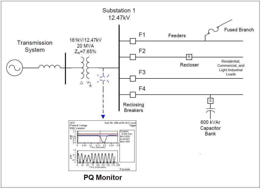
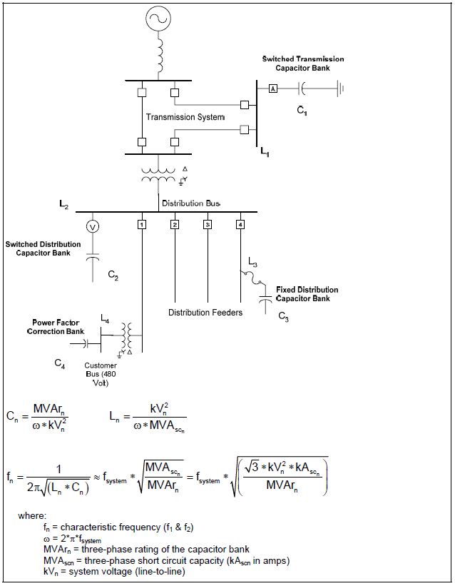
A voltage variation measurement analysis case study was completed for the 12.47 kV utility system shown in Figure 1. The utility substation included a 20 MVA, 161 kV/12.47 kV step-down transformer and a number of distribution feeders that supplied a mix of residential, commercial, and light industrial customers. In addition, one of the feeders had a switched 600 kVAr power factor correction capacitor bank.
MEASUREMENT RESULTS
The three-month monitoring period was from January 1, 2009 thru March 31, 2009. The power quality instrument used for the voltage variation measurements was the Dranetz-BMI Encore Series™. The instrument samples voltage at 256 points-per-cycle, current at 128 point-per-cycle, and follows the IEC 61000-4-3 method for characterizing measurement data. The measurement and statistical analysis was completed using the PQView® program.
Figure 1 – Illustration of Oneline Diagram for Measurement Data Evaluation
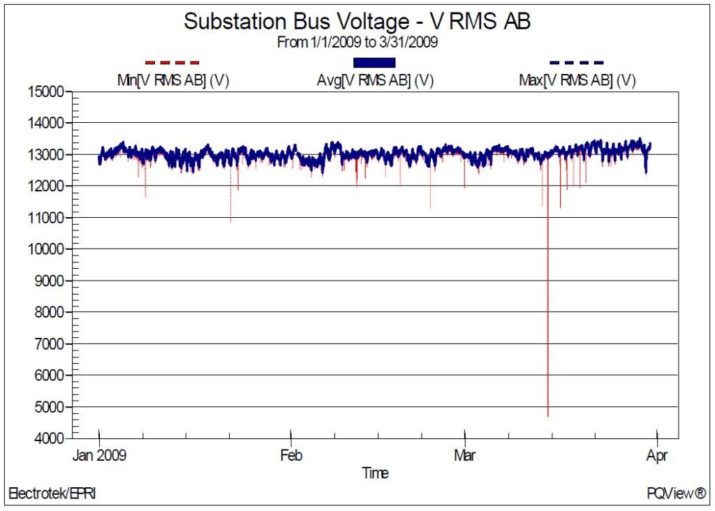
Figure 2 shows the measured rms voltage regulation trend on the 12.47 kV substation bus during the three-month monitoring period. One pole-mounted 600 kVAr distribution feeder capacitor bank was switched on-and-off each day using time clock controls in an attempt to maintain a relatively constant voltage profile. Statistical analysis of the 25,520 individual steady-state measurements yielded a minimum rms voltage of 12.427 kV, an average voltage of 13.022 kV, and a maximum voltage of 13.499 kV. In addition, the CP95 value was 13.277 kV (106.5% of nominal). CP95 refers to the cumulative probability, 95th percentile of a value.
Figure 2 – Measured Substation Bus Voltage Trend
Figure 3 shows the measured negative sequence voltage unbalance trend on the 12.47 kV substation bus during the three-month monitoring period. Statistical analysis of the 25,520 individual steady-state measurements yielded a minimum value of 0.244%, an average value of 0.492%, a maximum value of 0.894%, and a CP95 value of 0.629%.
Voltage unbalance is a steady-state quantity defined as the maximum deviation from the average of the three phase voltages or currents, divided by the average of the three phase voltages or currents, expressed in percent. Voltage unbalance can also be quantified using symmetrical components. The ratio of the negative sequence (or zero sequence) component to the positive sequence component is used to specify the percent unbalance. The negative sequence (or zero sequence) voltages in a power system generally result from unbalanced loads causing negative sequence (or zero sequence) currents to flow.
The primary source of voltage unbalance less than two percent is unbalanced single-phase loads on a three-phase circuit. Voltage unbalance can also be the result of capacitor bank anomalies, such as a blown fuse on one phase of a three-phase bank. Severe voltage unbalance (greater than 5%) can result from single-phasing conditions. Voltage unbalance is most important for three phase motor loads. ANSI Std. C84.1 recommends that the maximum voltage unbalance measured at the service entrance under no load conditions should be 3%. Voltage unbalance greater than this value can cause significant motor heating and subsequent failures. Unbalance detection circuits may be used to protect induction motors from this condition.
Figure 3 – Measured Substation Bus Negative Sequence Unbalance Trend
Solutions to voltage unbalance include balancing single-phase loads (both utility and customer) on three-phase circuits, minimizing system impedance differences (e.g., transmission line transposing), and utilizing power electronic-based power conditioning devices, such as static VAr compensators and power line conditioners.
This case summarizes an investigation of rms voltage variations. Voltage variations, such as voltage sags and momentary interruptions, are often the most important power quality concern for customers. These conditions are characterized by short duration changes in the rms voltage magnitude supplied to the customer. The impact on the customer depends on the voltage magnitude during the disturbance, the duration of the disturbance, and the sensitivity of the customer’s equipment. Although utilities continuously strive to provide reliable power to their customers, a number of normal operating conditions may cause voltage variation events.
Voltage sags and momentary interruptions are inevitable on the electric power system. Many of these variations occur during faults on the power system, and since it is impossible to eliminate the occurrence of faults, there will always be voltage variations on customer systems. Other sources of voltage variations include unbalance, induction motor starting, and voltage flicker. Table 1 shows the rms variation event summary listing for the three-month monitoring period. The table shows the date-and-time for each event, as well as the phase-to-neutral voltage magnitude in both volts (kV) and per-unit and the event duration in both seconds and cycles.
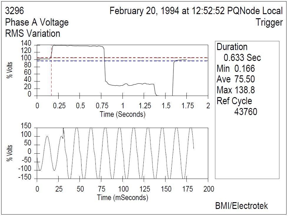
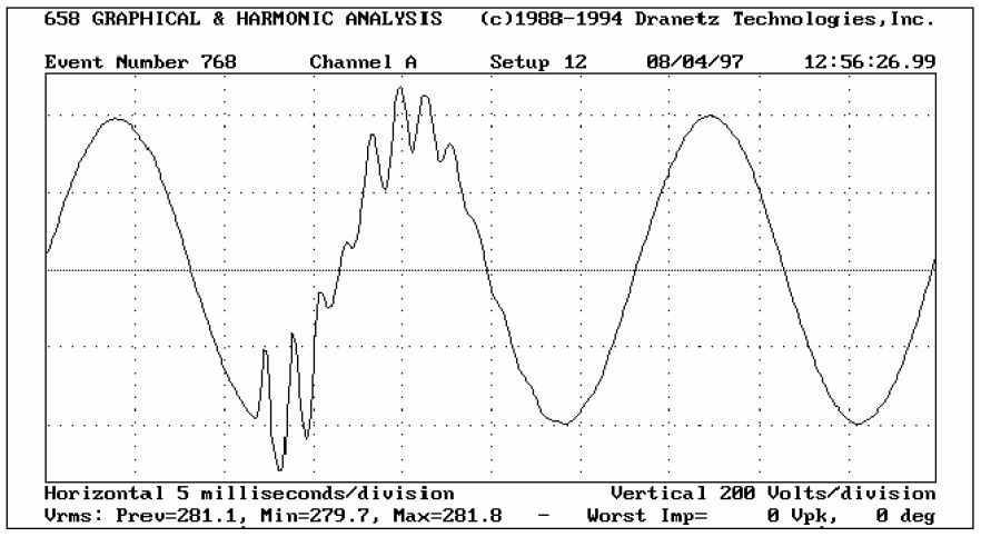
Figure 4 shows the corresponding waveform and rms characteristic for the worst-case voltage sag event measured during the monitoring period (Event #9). The magnitude of the voltage sag was 44.3% and the duration was 5 cycles. The voltage sag occurred during a thunderstorm. It was caused by a short-duration fault and subsequent fuse clearing on one of the distribution feeder branch circuits.
Table 1 – Event Listing for Measured RMS Variations
Event Number
Event Time
Magnitude (kVφN)
Magnitude (per-unit)
Duration (sec)
Duration (cycles)
1
1/8/2009 11:47:27.3300
5.587
0.776
0.058
3.5
2
1/22/2009 06:25:56.4200
5.863
0.814
0.058
3.5
3
1/27/2009 10:02:34.2140
5.943
0.825
0.075
4.5
4
1/27/2009 11:23:22.8930
6.136
0.852
0.067
4.0
5
1/28/2009 11:12:27.8920
5.631
0.782
0.092
5.5
6
2/1/2009 07:55:20.5900
6.401
0.889
0.175
10.5
7
2/11/2009 15:27:45.3340
6.146
0.854
0.158
9.5
8
3/13/2009 12:50:27.6560
5.132
0.713
0.075
4.5
9
3/14/2009 09:39:49.0670
3.189
0.443
0.083
5.0
10
3/14/2009 10:59:51.2400
3.708
0.515
0.117
7.0
11
3/24/2009 15:22:58.9810
6.436
0.894
0.108
6.5
Figure 4 – Measured Substation Bus Voltage Sag Event
When there are a significant number of events, it is generally not desirable to show the results for each individual measurement. One method for summarizing rms variation event data is to graph the magnitude and duration data on one single scatter plot. This method may also include an equipment tolerance (e.g., CBEMA) overlay. Figure 5 shows a summary of the events listed in Table 1 along with a CBEMA overlay. The graph also shows the number of events that are outside the equipment sensitivity characteristic.
Figure 5 – Measured Bus Voltage RMS Variation Magnitude Duration Characteristic
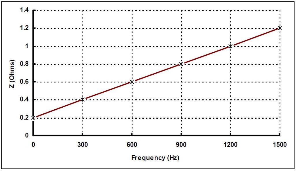
Voltage variation indices may be used to assess the service quality for a particular customer or utility system. One commonly used benchmarking value is known as SARFI, which stands for System Average RMS Variation Frequency Index. SARFI represents the average number of specified rms variation measurements that occurred over the assessed period. For example, SARFI70 is a measure of the number of voltage sags that can be expected with a minimum voltage below 70%. Another popular use of SARFI is to define the threshold as a curve. For example, SARFICMEBA would represent the number of rms variation events outside the commonly used CBEMA voltage tolerance envelope. The CBEMA curve was originally developed by the Computer Business Equipment Manufacturers Association. The curve was first published in IEEE Std. 446-1995.
The calculated SARFI values for the three-month monitoring period are summarized in Table 2. The SARFI90 value of eleven can be determined by counting the number of events in Table 2 with a voltage magnitude below 90%. In addition, the SARFICMEBA value of four that is shown in the table corresponds to the data previously shown in Figure 5.
Table 2 – Summary of RMS Voltage Variation SARFI Values
SARFI-CBEMA
SARFI-ITIC
SARFI-SEMI
SARFI-90
SARFI-70
SARFI-50
SARFI-10
4
2
1
11
2
1
0
Voltage sags are momentary undervoltage conditions. They are characterized by a decrease in the rms voltage (between 0.1 and 0.9 per-unit) at the power frequency for a duration of 0.5 cycles to 1 minute. They are typically caused by a fault somewhere on the power system. The voltage sag may occur over a significant area while the fault is actually on the system. As soon as a fault is cleared by a protective device (e.g., fuse), voltage generally returns to normal on most parts of the system, except the specific line or section that was actually faulted. The voltage magnitude during the fault is influenced by system characteristics, system protection practices, fault location and type, and system grounding.
Figure 6 shows the rms variation magnitude histogram for the three-month monitoring period. The cumulative frequency characteristic shows that a majority of the events had voltage magnitudes greater than 70%. Figure 7 shows a three-dimensional cross tabulation view of the rms variation measurements captured during the monitoring period and summarized in Table 1. The figure illustrates that a vast majority of the events had voltage magnitudes between 70-90% and durations that were less than five cycles.
The measurement results and customer equipment sensitivity were used to determine the appropriate mitigation alternatives. Equipment sensitivity is the primary factor that determines if a voltage variation event will disrupt a customer load or process. Some loads may be sensitive to just the magnitude of a voltage variation event, while other loads may be sensitive to both the magnitude and duration of the event.
Figure 6 – Measured Bus Voltage RMS Variation Magnitude Histogram
Figure 7 – Measured Bus Voltage RMS Variation Magnitude-Duration Summary
Power conditioning alternatives for voltage sags and momentary interruptions include a number of alternatives for utilities, customers, and equipment manufacturers. Determining which devices of an electrical load or process are sensitive to voltage variations will allow the selection of the appropriate type and rating for the power conditioner(s).
Modifications to the design of sensitive customer equipment may be the least expensive option, however, it is not always practical to implement. Modifying the utility system may also not be practical and may be, indeed, quite expensive. Power conditioning equipment, applied between the utility system and sensitive customer equipment, may be the most cost effective solution for voltage variation problems.
It is possible to make the equipment being used in customer facilities less sensitive to voltage sags and momentary interruptions. Clocks and controls with low power requirements can be protected with a small battery or large capacitor to provide greater ride-through capability. Motor control relays and contactors can be selected with less sensitive voltage sag thresholds. Controls can be set less sensitive to voltage sags unless the actual process requires an extremely tight voltage tolerance. This solution requires coordination with equipment manufacturers but the trend seems to be in the direction of increased ride-through capability. For instance, most programmable logic controllers use switched-mode power supplies that have a ride-through capability of about four cycles. Therefore, it should not be necessary to trip these controllers under short voltage sag conditions.
Since a vast majority of the measured rms variations events were short-duration voltage sags, the residential and commercial customers can use uninterruptible power supplies for their power conditioning solution. An uninterruptible power supply (UPS) is a power-electronic based device that provides a continuous voltage to a load by supplying power from a separate source when utility power is lost. A UPS is often used to protect computers, telecommunication equipment, or other critical electrical equipment where an unexpected power disruption could cause severe business disruption or data loss. A standby UPS (a.k.a., off-line UPS) with a ride-through range of 5 to 20 minutes will protect the sensitive equipment from most of the voltage sag events. This type of device is the most common configuration for commodity UPS units available at retail stores for the protection of small computer and entertainment system loads.
Industrial customer mitigation options include constant voltage transformers (CVTs), coil-lock devices, uninterruptible power supplies, magnetic synthesizers, dynamic sag correctors (DySC), dynamic voltage restorers (DVR), and motor-generator sets. Customers have the option to protect their equipment from voltage variation phenomena at a number of locations, including the point-of-entry and point-of-use. Generally, a combination of point-of-entry and point-of-use devices will provide the greatest level of protection.
Many voltage sag conditions for the industrial customers can be addressed by using constant voltage transformers. CVTs are especially attractive for constant, low power loads. Variable loads, especially with high inrush currents, present more of a problem for CVTs because of the tuned circuit on the output. A typical CVT circuit is shown in Figure 7. CVTs are an attractive option because they are relatively maintenance free, with no batteries to replace or moving parts to maintain. They are particularly applicable for industrial process control devices such as programmable logic controllers, motor starter coils, and the electronic control circuits of adjustable-speed drives. The negative aspects of CVT applications are efficiency (heat), size, weight, and availability in limited rating ranges. In addition CVTs have difficulty with dynamic and harmonic rich loads often requiring significant over rating. Over rating provides better performance and sag correction, but with a penalty of less efficiency, size, weight, and cost.
Figure 8 – Schematic for a Constant Voltage Transformer
SUMMARY
This case study presents a voltage variation data analysis for a 12.47 kV substation monitoring location for a three-month period. The analysis included trends of the rms voltage and unbalance and statistical analysis of the rms variation events. The results of the analysis showed that most of the events were short duration voltage sags. Constant voltage transformers, coil-lock devices, magnetic synthesizers, and a number of power-electronic based power conditioners may be used for protection against voltage sag events.
Voltage sag protection may be implemented on a single coil or piece of equipment. Correction may also be chosen for large portions of a facility or even for the entire facility. The selection of voltage sag mitigation will consist of engineering aspects as well as a cost versus benefit evaluation. The most cost-effective customer power conditioning solutions for this case were uninterruptible power supplies and constant voltage transformers.
The case showed that power quality monitoring can be used to characterize voltage variations at various locations on utility and customer power systems. The length of the monitoring period is dependent on the nature of the power quality problem. For example, voltage flicker trends may be collected over several days or weeks, while voltage sag and momentary interruption levels may need to be monitored for months, or even years to show the influence of seasonal variations. The monitoring period for this study was three months. Additionally, the objectives of a monitoring program determine the choice of measurement equipment, method of collecting data, disturbance thresholds, data analysis requirements, and the overall effort required.
REFERENCES
IEEE Recommended Practice for Monitoring Electric Power Quality,” IEEE Std. 1159-1995, IEEE, October 1995, ISBN: 1-55937-549-3.
IEEE Recommended Practice for Emergency & Standby Power Systems for Industrial & Commercial Applications (IEEE Orange Book, Std. 446-1995), IEEE, ISBN: 1559375981.
American National Standard for Electric Power Systems and Equipment – Voltage Ratings (60Hz), ANSI Std. C84.1-2006, National Electrical Manufacturers Association, December 2006.
Published by J. Mindykowski2, E. Szmit1, T. Tarasiuk2 1 Polish Register of Shipping, Electrical and Automation Department 2 Department of Marine Electrical Power Engineering of Gdynia Maritime University
1.Introduction
The issue of electric power quality onboard ships has seemed of utmost importance, in particular nowadays when a great progress in implementation of electric drives for ship’s thrusters, propellers and other smaller drives is evident. Ship’s electric power systems are isolated power systems. Similar systems are installed on aircraft, oil platforms and small islands, in industrial plants with seasonal character of operation and also as emergency electric supply systems in banks, hospitals, hotels, large supermarkets and skyscrapers [1], [2]. Characteristics of those systems are: scarce in other cases proportion of single consumer power to electric source power (some consumer powers are often comparable to generator power supplying them) [3] and relatively high short-circuit impedance of generators installed in the systems under consideration [1]. Finally, electromagnetic disturbances observed in isolated power systems are more serious than those observed in large connected systems in their normal operation. What is unique in ships power systems ? Answer is simple. System is installed on mobile object – the ship – and simultaneously is deciding for its operational control. Effects of incorrect system operation can be very serious and consequences of ship’s casualties are known very well from the news. Indeed, question of the electromagnetic disturbances determining electric energy quality in ship’s power systems has not only technical aspect and / or vessel operational safety. Paltry quality of electrical energy on ships has also its economic dimension. In spite of relatively not big power (normally no more than few MVA) of a single electric plant, large number of ships (30 395 of 1000 gt and above as of 1.01.2003 [4]) shows the measure of presented problem excellently.
2.Electromagnetic disturbances in ship’s power networks
Wide spectrum of electromagnetic disturbances, radiated and conducted, is present in the ship’s electric networks causing disorder in their element operation. Typical conducted, and particularly prolonged disturbances, as:
voltage and frequency variations;
voltage asymmetry;
distortions caused by harmonics, inter-harmonics, transient pulse disturbances;
improper distribution of active and reactive power between generating sets working in parallel.
The disturbances introduce many difficulties into operation of the ship’s crew and owner’s technical service, independently on basic value – the ship’s safety. Electric and electronic devices, the power network elements are the “causes” of disturbances and at the same time the “victims” of the waveform distortions. Ragged design and carrying out of installation give rise to the EMC disturbances, often causing the asymmetry and voltage level changes. Switching process in distribution switchgears and electrical consumers and also overvoltage during fuse blow out were traditionally causes of signal distortion in power network. Presently distortions are caused by still more popular power electronic converting systems used in machinery auxiliary drives, but not only. Drives consisting of power converters are applied to thrusters, big technological consumers and main propellers of the vessels. Marine generating sets are “weak” power sources (with 15-20 % impedance) compared to “stiff” sources (4-6 % impedance) more common in land industrial applications.
Converters of electrical power in co-operation with so weak power sources generate harmonic and inter-harmonic distortions causing inadmissible disturbances in power system. Distortions 15% and even 20% and above were observed onboard ships many times [5], [6], [7].
The examples of all above mentioned disturbances, i.e. voltage and frequency deviations, voltage asymmetry and distortions of voltage waveform are shown in Fig 1 to 5. Presented examples are the original results of some tests which were carried out on ships by personnel of Marine Electrical Power Engineering Department of Gdynia Maritime University. The test purpose was to settle the real voltage parameters (in fact its quality), supplying Main Distribution Boards of examined ships.
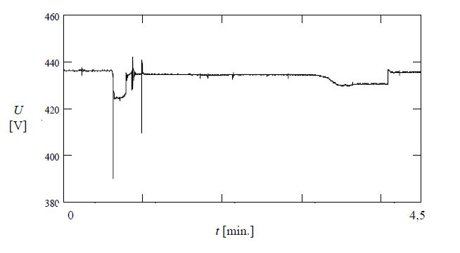
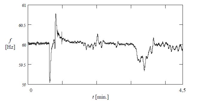
Fig. 1 represents variations of voltage rms value during the start-up and running of the thruster driven by 1,3 MW electric motor, when two generators with power 1,75 MVA each operated parallel. In that case overload of ship’s electric power plant had caused automatic switching off a less important services and next switching on the third generator with the same power, for parallel operation. Fig. 2 shows frequency variations for that case accordingly.
Fig. 1 Voltage variations during starting and running of the thruster [3]
Fig. 2. Frequency variations during starting and running of the thruster [3]
Voltage asymmetry in the system with nominal parameters Un=440 V and fn=60 Hz is shown in Fig. 3. Presented voltage asymmetry is so interesting because one can see harmonic distortion and pulse interference, too. Phenomena observed in that example were caused by shaft generator with power converter working on ship’s network with simultaneous failure of harmonic filter (3-phase LC passive filter).
Rys. 3 Voltage asymmetry (3,7%) [8]
Next two presented samples are also from the ship equipped with shaft generator working in network through power converter. However in that case all system components were operating correctly. Fig. 4 shows voltage inter-harmonic and harmonic distortion, e.g. interharmonic quantity is ca. 0,4% at frequency ca. 150 Hz when total harmonic distortion THD amounts 4,4% on Main Distribution Board 220 V bus-bars. It means that between power converter and the connection point of measuring apparatus, transformer attenuating commutation over-voltage was present. Fig. 5 shows the same measurement however measuring instrument was connected directly to 440 V bus-bars. In that case one can see the notching caused by commutation over-voltage in power converter. The THD coefficient amounts 13,5% for that case.
Fig. 4. Un=220V voltage inter-harmonic and harmonic distortion [9]
Fig. 5. Un=440V voltage pulse interference [9]
Finally, it is worth to present an example of distribution of active power between generating sets working in parallel. Such an example registered during ship manoeuvring has been shown in Fig. 6. There have been two generating sets working in parallel during analysed phenomenon. The active power load of generating set no 2 (PG2) has been depicted by bold line.
Fig. 6. Exemplary changes of active power load of respective generating sets working in parallel during ship manoeuvring.
It should be stressed that improper distribution of the active (as well as reactive) load can be hazardous. It may cause artificial overload and real collapse of whole supply system (switching operating generators off). The possible risk, especially during manoeuvring, can be hardly overstated.
The last of presented examples (Fig. 6) results from joint research of Marine Electrical Power Engineering Department of Gdynia Maritime University and Electrical and Automation Department of Polish Register of Shipping.
3. Harmonic distortions cause a lot of damages in electrical power system
Harmonic distortions can cause following typical damages to and malfunction of most elements and units of ship’s power network [10]:
Electric power sources:
Overheating and, in result, damage to bearings, winding and sheets packages of generators, because of a premature thermal ageing of insulation.
Electrical power consumers:
Overheating of the stator and rotor of fixed speed electric motors, risk of bearing damage because of the motor high temperature, additional rises of insulation temperature and its premature thermal ageing. A special hazard is present in the case of explosion proof motors operating in explosion hazardous areas. Unintentional tripping of circuit-breaker protections, interference with all control, electrical and electronic systems including radio- navigation and communication equipment, lighting, etc.
Electrical energy networks:
Overheating of cables as result of decreased ability to carry rated current because of reduction of effective cable cross section area by so called skin effect, also risk of cable damage due to resonance.
Overheating and premature thermal ageing of transformer sheets packages and winding insulation. It is important that harmonic distortion are present together with voltage and frequency variation and also voltage asymmetry, most frequent. Fig. 3 shows it. Negative synergy effect of above mentioned phenomena can be expected for many power consumers. That kind of interference synergy was discovered in tests of temperature rises in induction motor windings at different supply conditions [11].
4. Harmonic distortion – the past and the present time
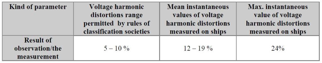
Ian C Evans, author of “Harmonic Mitigation for AC Thruster & Small Propulsion Drives”, advises that one of the classification societies have noted 24% voltage distortion (UTHD) in an offshore installation tested. He also says that voltage distortion of 12 – 19 % is relatively common, albeit not continuous in these installations, where up to 85% of the electrical load consists of electric drives [6, 7]. Distortion level measured on ships’ bus-bars by Department of Marine Electrical Power Engineering of Gdynia Maritime University are described in [3, 9, 11] and confirm international observations. However, the classification societies determined harmonic distortion limit on 5-10% level recognising possibility of serious faults of the electric network and, in result, general safety of the ship [14, 15].
Table 1. Results of voltage distortions measured in different vessels [5], [6], [7], [9]
It shows, a gap is between ships practice and classification societies attitude. Problem is that, classification societies determining harmonic level limits did not assign the method of their testing onboard. However, the limits of electric power disturbances were stated when the risk caused by power-electronic elements and systems was not present. DC driving systems not generating so serious interference had dominated on ships at that time
5. Harmonic mitigation – the present time and the future
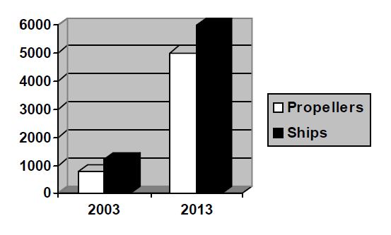
Global forecasts give information about several times growth of power electronic (measured in the million USD of installed “electric” propeller value or “electric” ship’s number) [7]. It enhances the issue.
Fig. 7 Global forecast of ship’s electric drives application
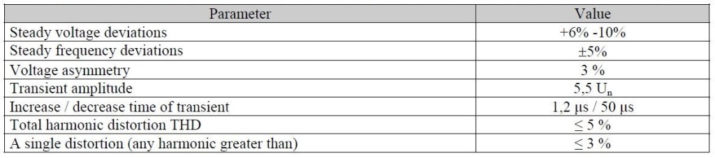
Individual classification societies have to revise their rules in connection with the fast development of the AC drives introducing many of harmonic and inter-harmonic distortions. These is the opinion of classification societies, marine electricians and electrical equipment producers. Recently some modifications of industrial standards were done. Many of the IEC and IEEE standards concerning permissible levels of electrical power parameters determining its quality and measuring methods are present now [16], [17], [18]. Polish and international standard PN-IEC 60092-101 “Electrical installations in ships – Part 101: Definitions and general requirements” has also set up many limits of quality parameters of electrical power [19]. Some exemplary parameters of that standard are placed in Table 2
Table 2. Chosen quality parameters of electrical power stated by PN-IEC 60092-101 standard
However none of classification societies have implemented many of that parameters into their rules up to now. Continuous monitoring of electric power quality is not also carried out onboard, presently. Sometimes some observations, occasional measurements are being carried out but they are not adequate solution because of large variation of power quality parameters during ship’s operation. It is worth to note that some producers of power system control devices are introducing some means of power quality verification but it can not be considered as a global solution.
The expected development of electric drives for ship propulsion is the next and new challenge for marine specialists. Therefore, it is necessary to introduce special requirements for electromagnetic interference prevention (by correction of energy parameters in ship’s electrical power system) and their effects (by increasing of consumers immunity) and also to monitor power quality in ship’s networks. Possibility of current control has appeared with the development of transducer technology and advanced method of electrical signal processing and also specialised devices for real time data processing. High yet prices of suitable systems are decreasing continuously (cost of signal processor amounts from a few to a several hundred dollars) [10].
6. Conclusion
Tests, studies and analysis carried out during research onboard ships indicate necessity of complex solution of power quality problem in ships power systems, unequivocally. Specific means to prevent against electromagnetic disturbances and their effects are required. It may be done by correction of power quality in ship’s power systems and improvement of the electric consumers’ EMC immunity. On the other hand monitoring of electrical power quality is needed. Therefore problem of electrical power quality and its assessment should be one of priority in designing, construction, classification and utilisation of ship’s electric systems, now and in the future. It is evident that on the one hand the matter applies to shipyards and ship’s owners and on the other to classification societies surveying ships production and exploitation processes [20].
Suitable solution of that problem requires sufficient knowledge and experience. The preparation of appropriate staff for shipyards, owners and classification societies, as well as research of new methods and ways to limit the influence of poor power quality on the effective economically and safe operation of ships are the tasks of maritime universities.
Bibliography: [1] De Abreu J.P., De Sa J.S., Prado C.C.: Harmonic voltage distortion in isolated electric systems. 7th International Conference “Electrical Power Quality and Utilization” Kraków, 17-19 September 2003, pp. 469-472. [2] Dzwonkowski A.: Niezawodność zasilania wybranych obiektów przemysłowych o sezonowym charakterze pracy. Przegląd Elektrotechniczny Nr 6/2003, pp.452-456. [3] Tarasiuk T.: Analiza metod i układów do wyznaczania wskaźników jakości energii w okrętowych systemach elektroenergetycznych. Rozprawa doktorska, Politechnika Gdańska, Gdańsk 2001. [4] Shipping Statistics and Market Review Institute of Shipping Economics and Logistics Nr 4, April 2003 [5] Reinecke H., Schild W.: Harmonics in main electric supply systems with semiconductor rectifiers and subsequent methods of compensation. IMECE’91 China, pp. 1-10. [6] Evans Ian C: Harmonic Mitigation for AC Thrusters & Small Propulsion Drives. The Harmonic Solutions Co. Uk. [7] Evans Ian C: Electric Ships, The future is electric, Driving ahead – the progress of electric propulsion The Motor Ship, September 2003, pp. 28-33. [8] Dudojć B., Mindykowski J.: Pomiary diagnostyczne filtrów harmonicznych jako instrument do poprawy jakości energii w sieciach okrętowych. Prace Naukowe Katedry Elektroenergetyki Okrętowej; Zeszyt monograficzny 1997, pp. 120-131. [9] Mindykowski J., Szweda M., Tarasiuk T.: Measurement equipment for ships electrical power systems; Proceedings of the 20 th IEEE Instrumentation and Technology Conference, Como, Italy 2004, pp. 1367-1372. [10] Szmit E., Mindykowski J., Tarasiuk T.: Zaburzenia elektromagnetyczne na statkach to wspólny problem armatorów, stoczni, uczelni morskich i towarzystw klasyfikacyjnych. Budownictwo Okrętowe, No 3/2004 March 2004, pp. 30-31. [11] Gnaciński P., Mindykowski J., Tarasiuk T., Influence of electrical power quality on induction cage machine durability. 7th International Conference “Electrical Power Quality and Utilization” Kraków, 17-19 September 2003, pp. 455-462. [12] Polski Rejestr Statków – Publication 11/P “Environmental tests of marine equipment”, Gdańsk 2002. [13] IACS Unified Requirements – E10 “Testing procedure for electrical, control and instrumentation equipment, computers and peripherals covered by classification. IACS Blue Book [14] Lloyds Register – Classification of Ships Rules and Regulations, Part 6 “Control, Electrical, Refrigeration and Fire”, January 1998. [15] Germanischer Lloyd – Rules for Classification and Construction, Volume I Part 1 “Seagoing Ships” Chapter 3 “Electrical Installations”, Edition 1998 [16] PN-EN 6100-2-4 “Electromagnetic compatibility EMC) Part 2: Environment Section 4: Compatibility levels in industrial plants for low frequency conducted disturbances”. [17] IEC 61000-4-30 “Electromagnetic Compatibility (EMC): Testing and Measurement Techniques – Power Quality Measurement Methods”. [18] IEEE 1159:1995 IEEE “Recommended Practice on Monitoring Electric Power Quality”. [19] PN-IEC 60092-101 “Electrical installations in ships – Part 101: Definitions and general requirements”. [20] Szmit E., Mindykowski J., Tarasiuk T.: Jakość energii elektrycznej na statkach wspólnym problemem armatorów, stoczni, uczelni morskich i towarzystw klasyfikacyjnych. Fair of Electrical Engineering, Electrical Power Engineering and Lighting Techniques “Electric Wiring”, session “Electrical Power Quality”, Proceedings edited by Stowarzyszenie Elektryków Polskich Oddział Gdańsk, Gdańsk 2004, pp. 23-30.
Published by Electrotek Concepts, Inc., PQSoft Case Study: Distribution Feeder Voltage Sag Evaluation, Document ID: PQS0905, Date: October 15, 2009.
Abstract: This case study shows the results for simulations completed to evaluate the impact of a distribution feeder fault on the operation of a customer adjustable-speed drive during the resulting voltage sag and momentary interruption. The simulations for the case were completed using the PSCAD program. A voltage swell on the feeder primary is also illustrated. The potential solution of increasing the dc link capacitance for the adjustable-speed drive was shown to be effective for the simulated conditions.
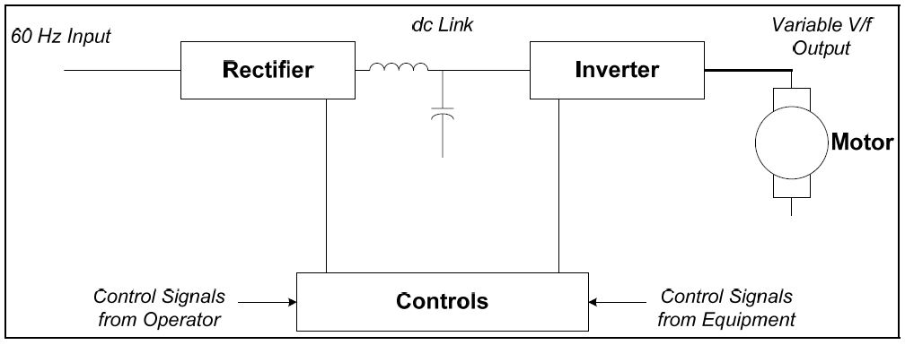
INTRODUCTION
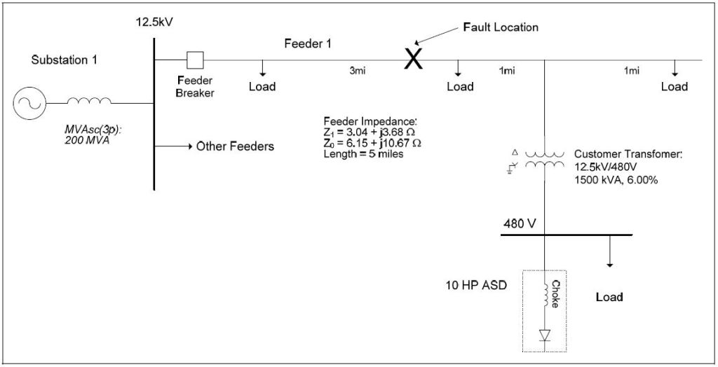
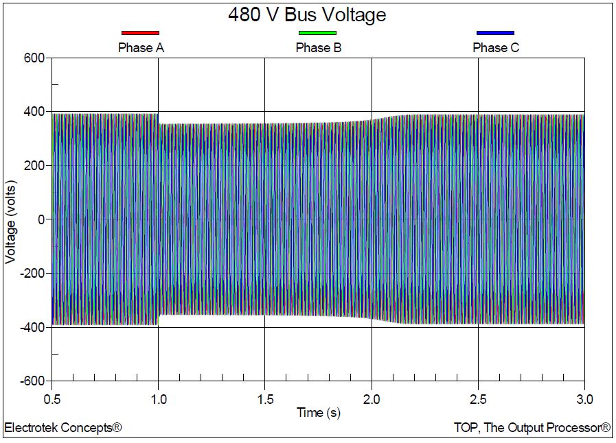
A distribution feeder voltage sag evaluation was completed for the system shown in Figure 1. The simulations for the case study were completed using the PSCAD program. The case involved simulating a voltage swell/sag/interruption event during a fault on the 12.5kV distribution feeder and then determining the dc link voltage for a typical customer adjustable-speed drive. An example of a representative measured voltage waveform is shown in Figure 2.
The accuracy of the simulation model was verified using three-phase and single-line-to-ground fault currents and other steady-state quantities, such as feeder and customer load currents. The circuit modeled for the case involved a 5-mile, 12.5kV distribution feeder supplying a 1500 kVA customer step-down transformer (12.4kV/480V).
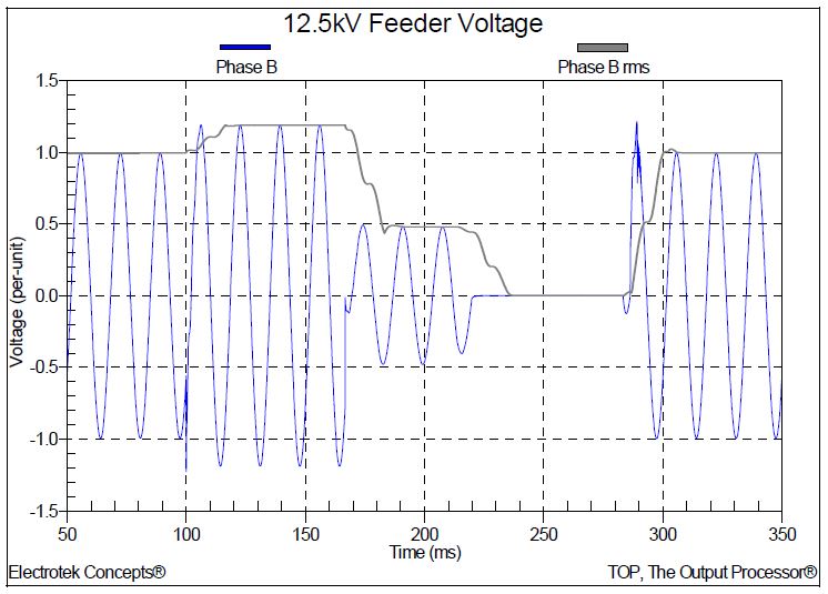
The waveform shown in Figure 2 illustrates a voltage swell, a voltage sag, and an interruption. A voltage swell is an increase in rms voltage magnitude above 1.1 per-unit for a duration of 0.5 cycles to 1 minute. Voltage swells are much less common than voltage sags and the magnitudes are not usually severe.
The most common cause of a voltage swell is a single-line-to-ground fault. During a single-line-to-ground fault, the voltage magnitude on the unfaulted phases can increase due to the zero sequence impedance. On an ungrounded system, the voltage on the unfaulted phases can be as high as 1.73 per-unit. On most systems, the voltage swell is less than 1.40 per-unit.
The simulated event began as a single-line-to-ground fault for 4 cycles and then evolved into a phase-to-phase fault for an additional 3 cycles. The feeder circuit breaker opened after approximately 11 cycles and reclosed after a 4-cycle delay. These switching times were selected to approximate the characteristics from the measured waveform. During the single-phase fault, a voltage swell occurs on the other two healthy phases. A voltage sag occurred during the phase-to-phase fault and a momentary interruption occurred while the circuit breaker was open.
Figure 1 – Oneline Diagram for Distribution Feeder Voltage Sag Evaluation
Figure 2 – Measured Voltage Swell and Interruption Waveform
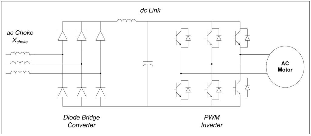
In addition to the voltage swell and voltage sag event on the distribution feeder primary, a customer transformer was modeled so the voltage on the 480-volt bus could be determined. A typical 10 hp adjustable-speed drive was included in the simulation model to determine the potential for nuisance tripping of the drive due to an undervoltage on the drive’s dc link. The oneline for the drive model is shown in Figure 3.
Figure 3 – Customer Adjustable-Speed Drive Simulation Model
Voltage sags cause a decrease in the dc link voltage for an adjustable-speed drive. The drive will likely trip off-line if the voltage falls below the dc link trip voltage. During short duration voltage sags, it may be possible to support the dc link voltage using a larger dc link capacitor. The drive may also experience high inrush currents when the voltage is restored.
SIMULATION RESULTS
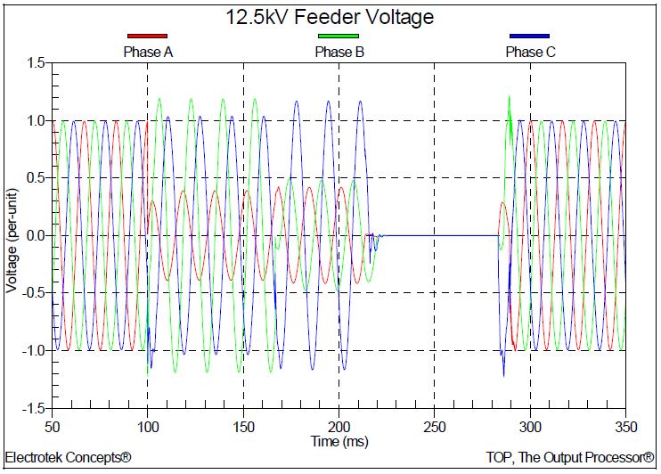
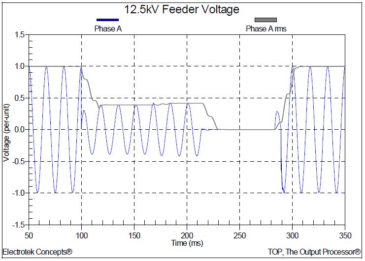
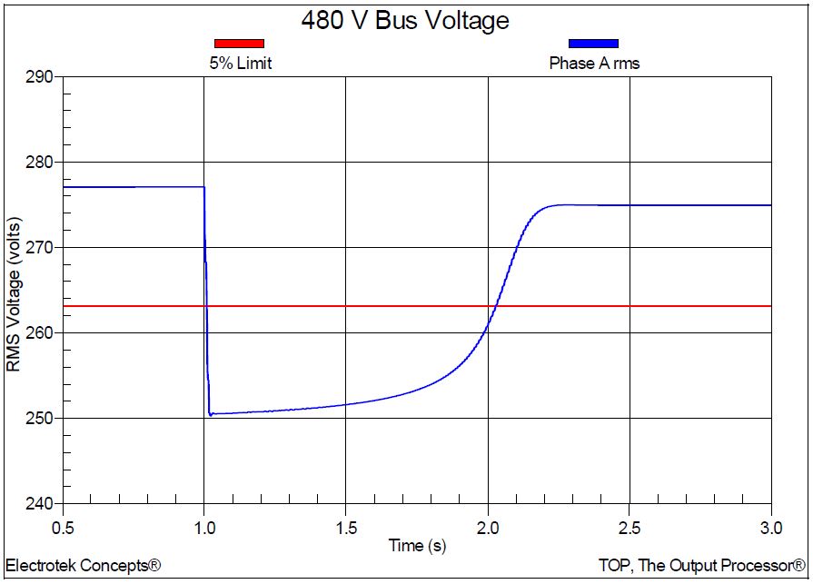
The simulated three-phase 12.5kV distribution feeder voltage is shown in Figure 4. The voltage swell, voltage sag, and momentary interruption are all contained in the one figure. The rms voltages for phases A and B are shown in Figure 5 and Figure 6, respectively. The rms voltage quantities were determined using a digital rms meter in the simulation program. The rms voltage characteristic of a voltage swell, followed by a voltage sag, followed by momentary interruption that was shown in Figure 2 is well represented with the simulation result shown in Figure 6.
Figure 4 – Illustration of Three-Phase Feeder Voltage during Fault Event
Figure 5 – Illustration of Phase A RMS Voltage during Fault Event
Figure 6 – Illustration of Phase B RMS Voltage during Fault Event
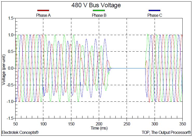
The resulting three-phase 480-volt customer secondary bus voltage is shown in Figure 7. The 12.5kV/480V step-down customer transformer is connected delta/wye-ground. For a single-phase fault on the primary of a delta/wye-ground transformer, the secondary phase-to-ground voltages would be 0.58, 1.00, and 0.58 per-unit, respectively. This is illustrated in Figure 7 during the initial portion of the event.
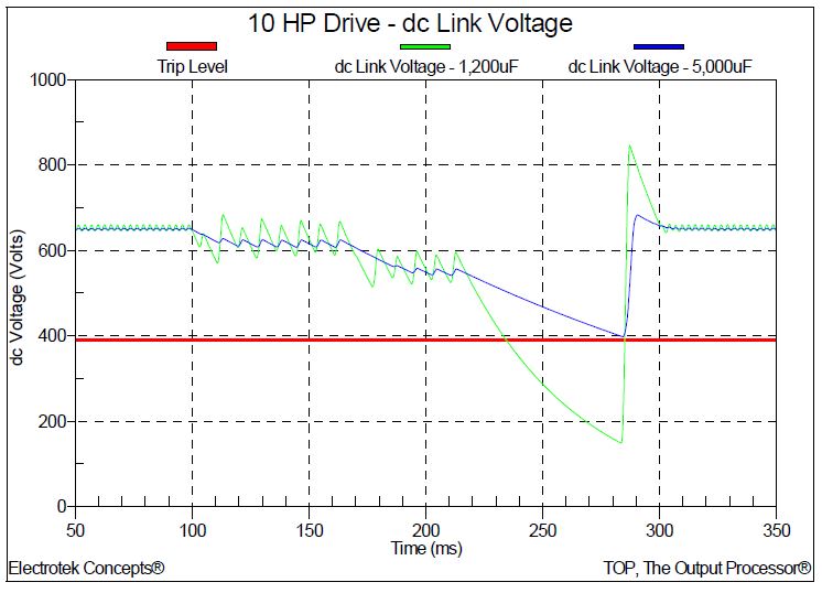
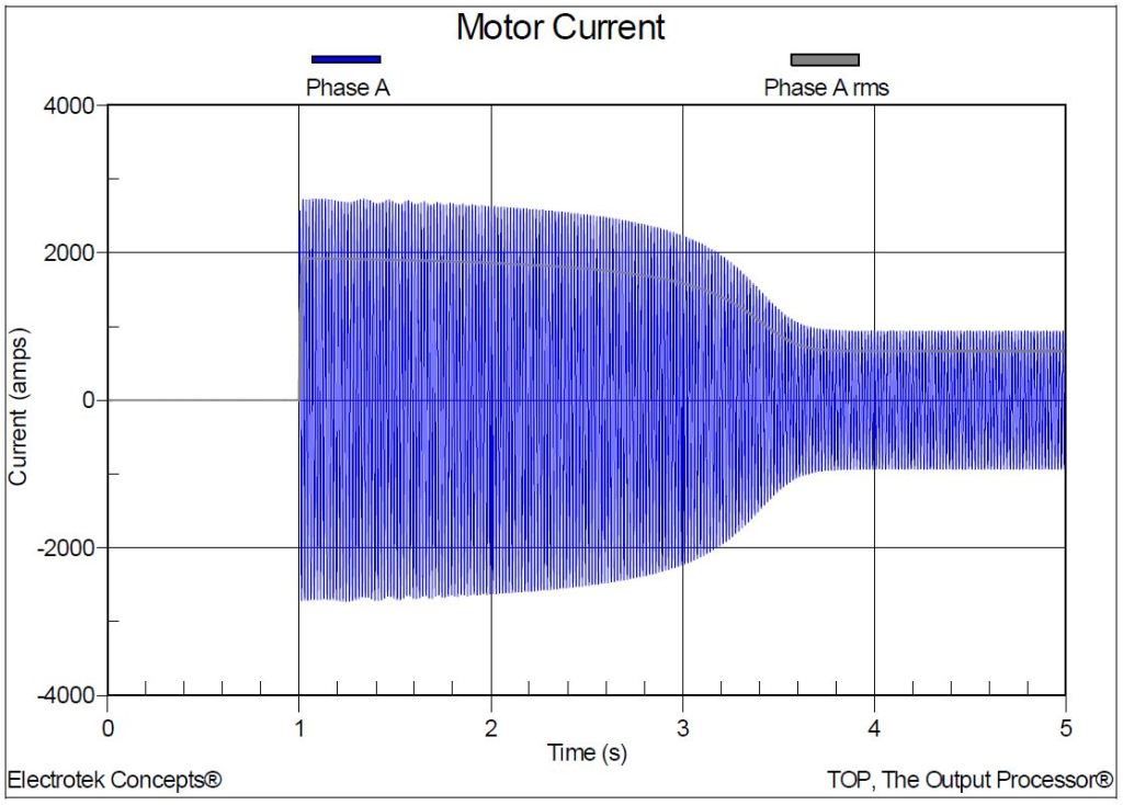
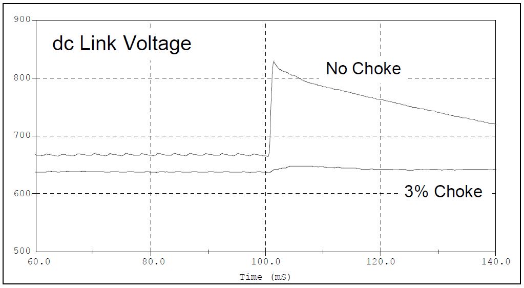
The resulting simulated dc link voltage for the typical 10 hp adjustable-speed drive is shown in Figure 8. The magnitude of the dc link voltage decreases during the voltage sag and momentary interruption. For this case, it was assumed that the dc bus low voltage trip voltage was 390 volts, which is 60% of the nominal 650-volt value.
Figure 7 – Illustration of Three-Phase Customer Bus Voltage during Fault Event
Figure 8 – Illustration of Drive’s dc Link Voltage during Fault Event
Figure 9 shows the simulation results for the case of increasing the dc link capacitance from 1,200μF to 5,000μF. The resulting simulated dc link voltage is slightly above the assumed undervoltage trip level so the drive does not trip for this condition.
Figure 9 – Illustration of the Effect of the dc Link Capacitance on the dc Link Voltage
SUMMARY AND CONCLUSIONS
This case study shows the results for simulations completed to evaluate the impact of a distribution feeder fault on the operation of a customer adjustable-speed drive during the resulting voltage sag and momentary interruption. A voltage swell on the feeder primary is also illustrated. The potential solution of increasing the dc link capacitance for the adjustable-speed drive was shown to be effective for the simulated conditions.
REFERENCES
IEEE Std. 1159-1995, IEEE Recommended Practice on Monitoring Electrical Power Quality, ISBN 1-5593-7549-3.
IEEE Std. 1159.3-2003, IEEE Recommended Practice for the Transfer of Power Quality Data, ISBN 0-7381-3578-X.
Published by U.S. Department of Energy (DOE), Office of Cybersecurity, Energy Security, and Emergency Response, Website: energy.gov
Image: U.S. Department of Energy (DOE), energy.gov
Power outages are common during disasters, and they can last for several days. You can reduce your losses and speed the recovery process with an emergency generator.
Portable generators made for household use can provide temporary power to a few appliances or lights. Commercial generators can help prevent service interruptions at businesses and critical infrastructure facilities, such as hospitals, water treatment facilities, telecommunications networks, and emergency response agencies. Federal, state, and local regulations may require you to obtain a permit to operate a generator. Make sure you follow these regulations when you operate and maintain your generator.
General Safety and Usage Guidelines for Backup Generators
Be sure to use your generator correctly. Using a generator incorrectly can lead to dangerous situations:
Carbon monoxide poisoning from engine exhaust. Even if you can’t smell exhaust fumes, you may still have been exposed to carbon monoxide. If you start to feel sick, dizzy, or weak while using a generator, get fresh air right away. If you experience serious symptoms, get medical attention immediately. Consider installing battery-operated carbon monoxide alarms. Be sure to read the manufacturer’s instructions and take proper precautions.
Electric shock or electrocution.
Fire.
Use a portable generator only when necessary, and only to power essential equipment.
Position generators outdoors and well away from any structure. Running a generator inside any enclosed or partially enclosed structure can lead to dangerous and often fatal levels of carbon monoxide. Keep generators positioned outside and at least 15 feet away from open windows so exhaust does not enter your home/business or a neighboring home/business.
Keep the generator dry. Operate your generator on a dry surface under an open, canopy-like structure and make sure your hands are dry before touching the generator. Do not use the generator in rainy or wet conditions.
Disconnect the power coming into your home/business. Before you operate your generator, disconnect your normal source of power. Otherwise, power from your generator could be sent back into the utility company lines, creating a hazardous situation for utility workers.
Make sure your generator is properly grounded. Grounding generators can help prevent shocks and electrocutions. Refer to OSHA guidelines for grounding requirements for portable generators.
Plug equipment directly into the generator. Use heavy-duty, outdoor-rated extension cords that are in good working condition and have a wire gauge that can handle the electric load of any connected appliances.
DO NOT plug the generator into a wall outlet. NEVER try to power your house/business by plugging the generator into a wall outlet or the main electrical panel. Only a licensed electrician should connect a generator to a main electrical panel by installing the proper equipment according to local electrical codes. Make sure the electrician installs an approved automatic transfer switch so you can disconnect your home’s wiring from the utility system before you use the generator.
Maintain an adequate supply of fuel. Know your generator’s rate of fuel consumption at various power output levels. Carefully consider how much fuel you can safely store and for how long. Gasoline and diesel fuel stored for long periods may need added chemicals to keep them safe to use. Check with your supplier for recommendations. Store all fuels in specifically designed containers in a cool, dry, well-ventilated place, away from all potential heat sources.
Turn the generator off and let it cool before refueling. Use the type of fuel recommended in the manufacturer’s instructions.
Inspect and maintain your generator regularly. Check aboveground storage tanks, pipes, and valves regularly for cracks and leaks, and replace damaged materials immediately. Tanks may require a permit or have to meet other regulatory requirements. Purchase a maintenance contract and schedule at least one maintenance service per year, such as at the beginning of every hurricane season. Keep fresh fuel in the tank, and run the generator periodically to ensure it will be ready when you need it.
Disclaimer: Because every emergency is different and for your safety, follow the guidance from your state and local emergency management authorities and local utility companies. The information provided on the U.S. Department of Energy’s website is for general information and not an endorsement of any particular material or service. Before you engage in activities that could impact utility services, such as electricity or natural gas, contact your local utility company to ensure that your activities are done safely.
For additional resources, visit ready.gov or benefits.gov. State and local emergency management authorities and local utility companies may also provide helpful guidance.
Published by Electrotek Concepts, Inc., PQSoft Case Study: Customer Induction Motor Starting Evaluation, Document ID: PQS0904, Date: October 15, 2009.
Abstract: This case study shows the results for simulations completed to determine the severity of an undervoltage condition during starting of a customer induction motor starting. The simulations for the case were completed using the PSCAD program. The effectiveness of a primary resistor starter is also summarized.
INTRODUCTION
A customer induction motor starting evaluation was completed for the system shown in Figure 1. The simulations for the case study were completed using the PSCAD program. The case involved simulating an undervoltage condition during starting of a 500 hp motor on a 480-volt customer bus. An example of a representative measured voltage waveform is shown in Figure 2. The accuracy of the simulation model was verified using three-phase and single-line-to-ground fault currents and other steady-state quantities, such as motor full load current. The circuit modeled for the case involved a 230kV system supplying a 34.5kV distribution feeder that supplies a 1,500 kVA customer step-down transformer (34.5kV/480V).
Figure 1 – Oneline Diagram for the Induction Motor Starting Evaluation
Figure 2 – Example Motor Starting Voltage Waveform
Motor starting is one of the most common causes of voltage variations. An induction motor will draw several times its full load current during starting. This lagging current creates a voltage drop across the impedances of the system. If the started motor is large enough relative to the system short-circuit capacity, these voltage drops can produce severe voltage sags on the system. Even small and medium horsepower motors can have inrush currents that are six-to-ten times the normal steady-state current levels. Motor starting voltage sags can dim lights, cause contactors to drop out, and disrupt sensitive customer equipment. These voltage sags may also affect the motor starting itself, because severe voltage sags may prevent the motor from successfully starting. Motor starting voltage sags may persist for many seconds.
Relevant system and induction motor data for the case included:
Three-phase induction motor rating:
500 hp
Rated induction motor voltage:
480 V
Motor efficiency:
92.0%
Motor full load power factor:
90.0%
Motor full load slip:
2.0%
Motor full load current:
542 A
Motor three-phase rating:
450 kVA
Motor starting current (5.7 x IFL):
3089 A
Motor locked rotor kVA:
2565 kVA
Short-circuit current at motor terminal:
28 kA
Short-circuit kVA at motor terminal:
23280 kVA
SIMULATION RESULTS
For a full voltage start, the voltage drop in per-unit of nominal system voltage may be estimated using the following expression:
where: V(pu) = actual system voltage (per-unit) kVASC = system short-circuit kVA at motor (kVA) kVALR = motor locked rotor kVA (kVA)
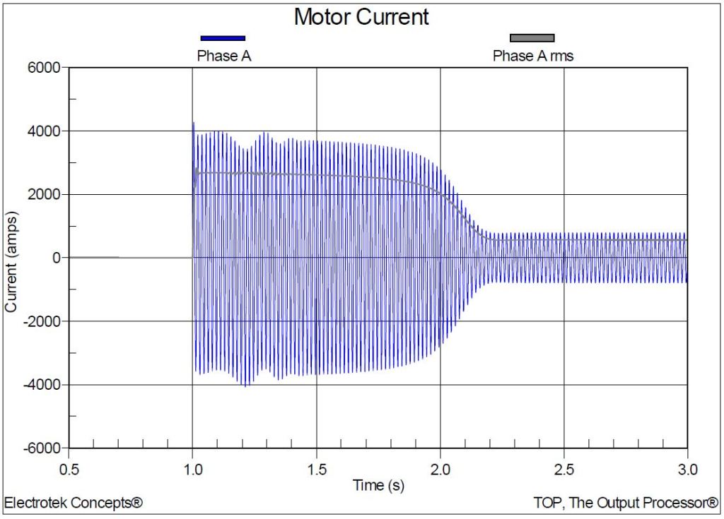
On a 480-volt bus, this rms phase-to-neutral voltage drop would be 249.6 volts. This full voltage starting condition was simulated in the first case. The phase A current is shown in Figure 3. The figure also includes the calculated rms current. The rms voltage and current quantities were determined using digital rms meters in the simulation program. The maximum simulated peak current for the full voltage start was 4275 A and the full load rms current was 565 A. The three-phase 480-volt bus voltage during full voltage motor starting is shown in Figure 4. The rms voltage is shown in Figure 5. The minimum rms voltage for the case was 250.3 volts, which is very close to the hand-calculated value of 249.6 volts.
Figure 3 – Illustration of the Full Voltage Start Motor Current
Figure 4 – Illustration of the Full Voltage Start Three-Phase Bus Voltage
Assuming that the maximum allowable voltage drop is 5%, the simulated 10% voltage drop for the full voltage starting case indicates that some type of mitigation is required. There are several motor starting techniques to limit the motor starting current including autotransformer starters, resistance and reactance starters, delta-wye starters, and shunt capacitor starters.
Figure 5 – Illustration of the Full Voltage Start RMS Bus Voltage
The second case investigated the effectiveness of a primary resistor motor starter to achieve the 5% voltage limitation. A primary resistor starter has one or more sets of resistors which are connected in series with the motor during starting. The resistors are typically bypassed by a contactor once the motor has reached full speed. Figure 6 shows the motor current for the case with a primary starting resistor. As can be observed from the figure, the magnitude of the starting current is lower than the full voltage case; however the motor takes somewhat longer to reach full speed.
Figure 6 – Illustration of the Primary Resistor Starter Motor Current
Figure 7 shows the simulated rms voltage for both the full voltage and primary resistor starter cases. The primary resistor starter reduces the magnitude of the voltage drop so that is very near the assumed 5% limit.
Figure 7 – Illustration of Voltage Drop for Full Voltage and Primary Resistor Starting
SUMMARY AND CONCLUSIONS
This case study shows the results for simulations completed to determine the severity of an undervoltage condition during starting of a customer induction motor starting. The effectiveness of a primary resistor starter is also summarized.
REFERENCES
IEEE Std. 1159-1995, IEEE Recommended Practice on Monitoring Electrical Power Quality, ISBN 1-5593-7549-3.
IEEE Std. 1159.3-2003, IEEE Recommended Practice for the Transfer of Power Quality Data, ISBN 0-7381-3578-X.
Published by Silicon Valley Power® (SVP), City of Santa Clara, California, USA.
Photo: Silicon Valley Power®
Power outages are inconvenient for everyone, and we at Silicon Valley Power (SVP) do everything we can to reliably maintain your power. When we do have an outage, SVP is dedicated to resolving the problem as quickly as possible. We take pride in being ranked among the top 10 percent of utilities in the nation for power reliability.
If the power does go out, here are a few things you can do to make sure that you, your family and those around you stay safe and sound.
Be Prepared
Visit the USDA food safety site or go to USDA.gov, look for “Food Safety,” print out the safety guidelines and tape them inside a food cupboard.
Have a cooler, and keep ice packs and/or containers of water stored in your freezer. During an outage, the ice packs can protect your food in the cooler, or they can be moved from the freezer to your refrigerator to help keep it cool.
Plan ahead and know where dry ice and block ice can be purchased.
Keep canned food on hand along with a hand-operated can opener.
Have flashlights and fresh batteries readily available to use during a power outage.
Emergency lights that turn on when the power goes off can be useful and can be found at any hardware store or online.
Plug electronic equipment into surge protectors to protect against a surge when power is restored.
Have a battery-operated radio and fresh batteries or hand-cranked radio available.
If you lose your power, you’ll want to be sure that the food in your refrigerator remains safe to eat for as long as possible.
Here are some valuable Food Safety tips from the U.S. Department of Agriculture:
Keep an appliance thermometer in the refrigerator and one in the freezer at all times. Built-in temperature displays may not function during an outage.
Keep meat, poultry, fish, and eggs refrigerated at or below 40 °F.
Keep frozen food at or below 0 °F.
Keep the refrigerator and freezer doors closed as much as possible. Check thermometers only when opening doors for another reason.
The refrigerator should keep food safely cold for about 4 hours if it is unopened.
If you have frozen ice packs or containers of water, you can place them in the refrigerator to help keep the temperature cool.
A full freezer should hold the temperature for approximately 48 hours (24 hours if it is half full) if the door remains closed. See the Food Safety guidelines for more information.
Know USDA guidelines about packing frozen food closely together in the freezer if the freezer is not full.
Stay Connected During a Power Outage
It is most likely that you will lose the connection to your home Internet equipment such as a router or modem, and certainly lose external power for your electronic equipment such as computers and TVs during a power outage. In addition, you may lose connection to external wireless and cell phone services.
The Federal Emergency Management Agency has tips that can help in an emergency. Here are some ideas that may help you maintain or regain connection to Internet access and/or cell phone service, if it is available, during a power outage:
Most mobile devices that are powered or charged using a USB cable require a 5-volt power source, not a 110-volt household outlet.
Most modern laptop computers have USB ports that provide 5-volt power. You can connect using the USB power cord that you normally use to charge your phone. Keep your laptop charged, as it can be a source to recharge your cell phone during an outage.
Your vehicle’s lighter outlet can provide numerous recharges for your cell phone using an inexpensive USB adapter. Connect the adapter using the USB power cord that you use for your phone.
An extra battery pack or solar battery pack for your cell phone is wise and inexpensive.
Unplug unprotected electronic equipment to protect against a power surge when electricity of restored, or use a surge protector.
Published by Anders Larsson and Math Bollen, ELFORSK, Elforsk rapport 09:29, October 2008
Summary
The frequency range from 2 to 150 kHz is not sufficiently covered in international standards. The contrast with the frequency range below 2 kHz is striking. There have traditionally been good reasons to emphasize on the lower frequency range, where the absence of mitigation measures would lead to serious problems.
For frequencies above 150 kHz, potential interference with public radio broadcasting has been the driving force for standardization.
In the frequency range 2 – 150 kHz no significant sources of emission used to exist. Also no widespread problems due to high disturbance levels in this range have been reported yet.
There are however two good reasons for turning the attention to this frequency range. The first is the use of (part of) this frequency range for power-line communication. The second is the increasing use of end-user equipment emitting conducted disturbances in this frequency range.
Based on the measurement of voltage and current distortion, three types of disturbances are recognized in the frequency range 2 to 150 kHz.
Narrowband signals appear mainly in the form of individual frequencies due to power-line communication.
Broadband signals are mainly due to individual end-user equipment with active power-factor correction.
Recurrent oscillations (typically every 10 ms) are due to limitations of the power-electronic converters around the current zero crossing.
For each of these disturbance types, compatibility levels, emission limits and immunity limits are needed to come to a working EMC framework. Proposals are made for narrowband and broadband signals. No proposal has been made for recurrent oscillations due to the lack of information available at the moment.
When power-line communication is used, some measured are needed against low impedance of non-communication equipment. This may be measures taken by the operator of the communication equipment on a case-by-case basis or requirements on the minimum input impedance of equipment in the frequency range used for power-line communication.
We propose to use the time domain for measurements throughout the frequency band 2 to 150 kHz.
1 Introduction
The frequency range from 2 to 150 kHz is not sufficiently covered in international standards. The contrast with the frequency range below 2 kHz is striking. There have traditionally been good reasons to emphasize on the lower frequency range, where the absence of mitigation measures would lead to serious problems.
For frequencies above 150 kHz, potential interference with public radio broadcasting has been the driving force for standardization.
In the frequency range 2 – 150 kHz no significant sources of emission used to exist. Also no widespread problems due to high disturbance levels in this range have been reported yet.
There are however two good reasons for turning the attention to this frequency range. The first is the use of (part of) this frequency range for power-line communication. The second is the increasing use of end-user equipment emitting conducted disturbances in this frequency range.
This document will give an overview of the existing standards in this frequency range and propose additional standardization towards a more complete set of standards. The proposals are based on a range of measurements of voltage and current disturbances in this frequency range.
2 The IEC concept of electromagnetic compatibility
The concept used in IEC for achieving electromagnetic compatibility in a system, including some of the terminology used, is shown schematically in Figure 2.1. A similar figure is shown in Annex A of IEC 61000-2-2 and in several other publications.
Figure 2.1, The IEC concept of electromagnetic compatibility.
The figure specifies a number of different levels and limits, which will be discussed briefly below1.
2.1 Compatibility level
The compatibility level is a reference level for coordinating emission limits and immunity limits. The term was originally introduced for radiated emission with one emitter and one suscepter. The compatibility limit would in that case be chosen as an economic balance between reducing emission and improving immunity.
1 For a detailed discussion of the various terms and existing standards, see: Math Bollen – Problembeskrivning och emission och immunitet, STRI rapport R08-470, February 2008. This report will also be available as an Elforsk report.
For equipment connected to the power system the situation is more complex. The electromagnetic environment to which a device is exposed is due to the emission of several to many individual devices and is also influenced by the way in which the disturbances propagate through the power system. For conducted disturbances the compatibility level has often been coordinated with the existing disturbance levels in the power system. Emission limits for individual sources are set in such a way that the disturbance levels do not exceed the compatibility levels.
2.2 Planning level
Planning levels are used by a network operator to prevent the disturbance levels from exceeding the electromagnetic compatibility levels2 or any levels set by a regulator. The choice of planning levels is up to the network operator, but they should obviously not exceed the levels set by the regulator. The planning levels are used among others to determine the need for additional mitigation measured when connecting new loads. The planning levels. being internal quality objectives used by the network operator, are not set by IEC, but IEC does give indicative planning levels for some disturbances at different voltage levels (harmonics and voltage fluctuations at MV level and higher).
2 One may argue that compatibility levels do not concern the network operator, but that planning levels instead should be compared with voltage characteristics. This discussion is out of the scope of this report.
2.3 Emission limit
According to e.g. IEC/TR 61000-3-6 is “emission limit” defined as the “maximum emission level specified for a particular device, equipment, system or disturbing installation as a whole, assessed and measured in a specified manner”. The latter part of the phrase (assesses and measured in a specified manner) is very important and the cause for many discussions and misunderstandings, within standard-setting groups as well as for those using the standards.
The equipment standards set a limit on the emission of a device, under strictly defined and controlled laboratory conditions. The reason for this is the need for being able to reproduce the results: the testing result should be the same for different testing labs.
A consequence of this is however that the emission in reality, i.e. when connected to a power system with many other devices connected, will be different and that it may exceed the emission limit. This is one of the reasons for the spread of “emission level of the system” in Figure 2.1. The intention of the emission tests is however that a device with an emission below the limit during the test will not cause emission widely exceeding the limit in reality. In other words: passing the test should be a guarantee for limited emission during practical use. Note that this is a guarantee mainly towards the network operator. Under the EMC directive, the manufacturer and user of the equipment are no longer responsible once the equipment has passed the required tests.
The emission limit sets the maximum disturbance level generated by equipment, often measured at the mains terminal of the equipment. These limits are normally set for a single source and one piece of equipment. The emission levels can be measured as a current or as a voltage against a standardized source impedance.
For harmonics in the frequency range up to 2 kHz, IEC 61000-3-2 sets limits for the current emission for each harmonic frequency. But for fast fluctuations in load current, the emission limit is set as a maximum Pst value against a reference impedance.
2.4 Immunity limit
This is defined in e.g. IEC/TR 61000-3-6 as, ”the maximum level of a given electromagnetic disturbance on a particular device, equipment or system for which it remains capable of operating with a declared degree of performance”.
The same restrictions hold for the immunity limit as for the emission limit discussed before: it holds only under well-defined laboratory conditions. A number of disturbances are defined in detail and the device is exposed to those. The underlying assumption is that if a device is immune to these “standard disturbances”, it will be able to cope with the majority of disturbances that occur in reality. It will be clear that this is not always the case and the discussion on this is ongoing both within standard-setting groups and within the wider power-quality community.
To make sure that the equipment can operate when connected to the grid together with other loads it is subjected to different test. Some typical tests could be dips, transients, voltage fluctuations, magnetic fields etc. For example, tests against harmonic voltage distortion are prescribed in IEC 61000-4-13.
3 Disturbances in the frequency range 2 to 150 kHz
Measurements have been performed of the voltage distortion to which equipment is exposed in the frequency range from 2 to 150 kHz. The results of these measurements are presented among others in [5][6][7]. This work and other publications have resulted in the following subdivision of disturbances occurring in this frequency range:
Narrowband signals;
Broadband signals;
Recurring oscillations.
These three types of disturbances will be described separately below. For each of these three types, emission, compatibility and immunity levels should be defined. The setting of these levels will be discussed in Chapters 4, 5 and 6.
Based on the compatibility levels, voltage characteristics and planning levels can next be chosen.
3.1 Narrowband signals
Narrowband signals appear mainly in the form of individual frequencies due to power-line communication. Also individual equipment may emit narrowband signals, but the resulting levels of voltage distortion remain well below the voltage signals used for power-line communication. Existing standards define the maximum emission levels for communication equipment in this frequency range. The compatibility level should be above this emission level. The immunity level of both communication and non-communication equipment should in its turn be above the compatibility level. This will be discussed further in Chapter 5.
3.2 Broadband signals
Broadband signals in the frequency range 2 to 150 kHz are mainly due to individual end-user equipment with active power-factor correction. Also expected future equipment like solar panels, microgeneration and chargers for hybrid-electric cars will most likely emit this kind of signals. The distortion is related to the switching frequency used in the power-electronic converters. The switching frequency however varies with time and is different for different devices so that the resulting voltage distortion has in many cases a broadband character.
It was shown that the emission of active power-factor correction circuits shows a complex time-frequency behaviour. However the resulting voltage distortion, being caused by the sum of many individual devices, has more of a broadband character even in time-frequency domain.
An example of emission due to a broadband signal is shown in Figure 3.1. The corresponding spectrum is shown in Figure 3.2. The oscillations that are visible in the time domain around the current maximum and minimum show up as a band in frequency from about 40 to 80 kHz.
Figure 3.1. Example of broadband signals: currents measured in a lighting installation; measured waveform (top) and high-pass filtered waveform (bottom).
Figure 3.2. Spectrum of the current shown in Figure 3.1, grouped into 200-Hz bands.
To analyse the sub-cycle variations in distortion neither the frequency domain nor the time domain is a suitable tool. Instead the time-frequency domain spectrogram has been proposed and successfully used for this [5][6][7]. Using a time-frequency description (like in the spectrogram) would introduce unnecessary complications for standardization purposes. The time-frequency domain remains a useful tool however for analysis of waveform distortion in the frequency range from 2 to 150 kHz.
By extrapolation of the requirements for harmonic voltage distortion just below 2 kHz, a safe level equal to 0.5% (of nominal voltage) per 200-Hz band has been concluded in [1] as a planning level. A compatibility level equal to or somewhat above this level could be appropriate. The immunity level should be chosen above the compatibility level.
Any emission levels should be chosen such that the resulting voltage distortion will not exceed the compatibility level for practical source impedances and number of devices. This will be discussed further in Chapter 6.
3.3 Recurring oscillations
These are for example due to limitations of the power-electronic converters resulting in oscillations around every voltage zero crossing. The frequency of these oscillations is a few kHz, amplitudes up to 20 Volt have been observed and they repeat every 10 milliseconds.
A measurement of recurrent oscillations is shown in Figure 3.3. The measurement was performed near a group of fluorescent lamps in a shop. The low-frequency components, including the power-system frequency, have been removed by means of an analog filter with a cut-off frequency of 2 kHz. The three traces correspond to the three phases. Oscillations are visible (in the form of spikes) in two of the three phases recurring every 10 ms. The oscillations are either absent or lost in the broadband signal in the third phase.
Figure 3.3. Measured high-pass filtered voltage in three different phases.
Measurements at many locations have shown that such recurrent oscillations are a common phenomenon. Their origin is shown in Figure 3.4: the current drawn by a fluorescent lamp with high-frequency ballast as measured in the Pehr Högström laboratory at Luleå University of Technology. The top trace shows the measured current, the bottom trace shows the high-pass filtered version. A digital filter with a cut-off frequency of 2 kHz has been used. The notches present in the non-filtered current are associated with oscillations when the current restarts. The presence of these notches is referred to in the power-electronics literature as “zero-crossing distortion” or “cross-over distortion”, hence the term “zero-crossing oscillations” to refer to these recurrent oscillations.
Figure 3.4. The current drawn by one fluorescent lamp (top) and the digital band-pass filtered version (bottom).
The reason for the importance of these recurrent oscillations is shown in Figure 3.5. The timing of the oscillations are linked to the zero-crossing of the current which in turn is linked to the zero-crossing of the voltage. As all equipment experiences the same voltage, the oscillations occur at the same time for all equipment. The result is that the magnitude of the oscillations increases with increasing number of devices. This is illustrated in Figure 3.5 showing measurements done in the Pehr Högström laboratory. The three traces show the current taken by one, three or nine fluorescent lamps. The increase in magnitude of the recurrent oscillations is obvious.
Figure 3.5. Filtered current with one (top), three (middle) and nine (bottom) lamps connected.
These recurrent oscillations form a new type of disturbance, for which neither characteristics, not limits exist. This will make it difficult to set standards. This will be discussed further in Chapter 6.
4 Narrowband signals
4.1 Existing limits
Maximum emission due to power-line communication is given in the form of voltage limits in EN 50065-1 and in IEC 61000-3-8. According to these standards is the signal considered as a narrow band signal if its bandwidth is less than 5 kHz. Voltage characteristics are given in EN 50160, where they are referred to “voltage levels of signal frequencies”.
The emission limits according to EN 50065 and IEC 61000-3-8 are reproduced in Figure 4.1. The two vertical lines indicate the frequency range of interest for this document (2 to 150 kHz). Note that the emission limits are expressed in terms of voltage. There is no reference impedance associated with this limit; the voltage after injection of the communication signal shall not exceed the indicated limit. For frequencies up to 95 kHz the limits are the same for both standards. EN 50065 does not cover frequencies above 150 kHz. IEC 61000-3-8 does give limits but these are an order of magnitude more restrictive than below 150 kHz. This is to prevent interference with commercial broadcasting (the long-wave band starts at 150 kHz).
Figure 4.1. Emission limits for narrowband signals according to EN 50065 (blue solid line) and IEC 61000-3-8 (blue dashed line). Up to 95 kHz the limits are the same. Voltage characteristics according to EN 50160 (green solid line).
The limit according to EN 50065 and IEC 61000-3-8 is at 134dBV (about 2% of 230 Volt) for frequencies between 3 and 9 kHz. The voltage characteristic according to EN 50160 is equal to 5%. The large margin between the emission limit and the voltage characteristic is possibly to allow for the presence of multiple devices and for amplification of voltage distortion due to resonances. According to the application guide for EN 50160 [10] the voltage characteristics are based on EN 50065-1 with a factor of two taken between the emission limit and the voltage characteristics.
At 100 kHz, the emission limit according to EN 50065 is at 120 dBV (about 0.5% of 230 Volt) whereas the voltage characteristic is at slightly above 1%. We see the same factor of two as before.
EN 50065-2-3 covers immunity requirements for power-line communication equipment operating in the range from 3 to 95 kHz. This document prescribes that a modulated 80-dBV signal is applied at “spot frequencies” between 3 and 30 MHz. The same test is specific in EN 50065-2-2 for the range from 9 to 148.5 kHz.
4.2 Proposed emission limits
We propose to use the existing emission limits for communication equipment as shown in Figure 4.1.
For non-communication equipment we propose to set the limit for narrow-band emission the same as the limit for broadband emission to be discussed in Chapter 5.
4.3 Proposed compatibility level
We propose to set the compatibility level equal to the voltage characteristic according to EN 50160 and shown in Figure 4.1 for frequencies up to 100 kHz. For frequencies between 100 and 150 kHz we propose to set the compatibility level at 130 dBV, independent of the frequency.
4.4 Proposed immunity level
We propose to set the immunity level for non-communication equipment 6 dB above the compatibility level.
5 Broadband signals
5.1 Existing limits
Emission limits for broadband signals by lighting equipment are given in CISPR 15. Those limits are reproduced as the blue solid line in Figure 5.1. The limits are given as a voltage against a reference impedance. Limits for the emission by power-line communication equipment at frequencies not used for communication purposes is given in EN 50065. For frequencies above 150 kHz those emission limits are the same as those in CISPR 15. Figure 5.1 also gives the voltage characteristics for narrowband signals, according to EN 50160, as a reference.
Figure 5.1. Emission limits for broadband signals according to CISPR 15 (blue solid line) and EN 50065 (dashed line). The voltage characteristics for narrowband signals (green solid line) are given as a reference.
The source impedance (referred to as “artificial mains network”) for the frequency range 9 to 150 kHz is given in CISPR 16-1-2 and reproduced in Figure 5.2. The source impedance increases from about 5 Ω at 9 kHz to 33 Ω at 150 kHz. Note that this impedance is intended to give the same precondition for measurement and by that give the same result wherever the measurements are made. The actual connection point may have a rather difference impedance as a function of frequency.
Figure 5.2. Source-impedance representation according to CISPR 16-2-1 (left) and impedance values for selected frequencies (right)
When quantifying the level of broadband signals it is important to indicate the bandwidth used. Both CISPR-16 and IEC 61000-4-7 (informative annex) give a bandwidth equal to 200 Hz. All levels and limits below are given per 200-Hz band.
5.2 Proposed emission limits
From the previous section it follows that emission limits only exist for lighting equipment and only in the frequency range 9 to 150 kHz. We propose to extend these emission limits to all devices equipped with an active interface. We also propose to extend the limits to the frequency band 2 to 9 kHz. The emission limits between 2 and 9 kHz should be the same as the limits between 9 and 150 kHz.
Recent measurements [3][11] have shown that the emission of individual equipment strongly depends on the presence of neighbouring equipment. This will have to be considered in the tests, without infringing on the requirement that the tests should be reproduceable.
5.3 Compatibility levels
A proposal for planning levels in the frequency range 2 to 9 kHz is presented in [1]. The planning levels for frequencies just below 2 kHz have been used as a starting point in [1]. Next the assumption is made that planning levels above 2 kHz should be the same as the ones just below 2 kHz. This results in a planning level equal to 0.5% (1.15 V).
The compatibility level should be equal to or higher than the planning level.
The emission limit (against a reference impedance) is equal to 0.3 Volt in the frequency range 9 to 50 kHz. It is recommended to use the same limit in the frequency range 2 to 9 kHz.
Using 1.15 V as a compatibility level gives a factor 3.8 between the emission and compatibility levels.
It is difficult to know, without much more detail about the emission source, how the emission from different sources will add. However, some estimations can be made. If we assume that emission is random between sources, about 14 emitters can be connected to the same locations before the compatibility level is exceeded, assuming the compatibility level is equal to the 0.5% and assuming that the source impedance is equal to the reference impedance.
If we assume that the emission of all sources is identical, about 4 units will result in the voltage disturbance exceeding the compatibility level.
For higher frequencies, above 9 kHz, no guidance exists for the choice of compatibility level. Therefore it is proposed to maintain a constant ratio between emission limit and compatibility level. This results in the following compatibility level
1.15 V between 2 and 50 kHz;
Linearly decreasing from 1.15 to 0.4 V between 50 and 150 kHz.
5.4 Proposed immunity limits
We propose to set immunity limits 6 dB above the compatibility level. This results in the following immunity limits:
2.3 V between 2 and 50 kHz;
Linearly decreasing from 2.3 to 0.8 V between 50 and 150 kHz.
Note that the immunity of equipment should be tested against a broadband signal with a spectrum as defined by the two bullet points above. It is not sufficient to generate individual frequencies as test signals, but the equipment under test should be exposed to all frequencies at the same time.
5.5 A final observation
The compatibility levels proposed in this chapter are to a large extent based on existing disturbance levels. The proposed limits are “safe limits” for which we are reasonably certain that no widespread interference will occur. However, there are voices that point to unexplained equipment maloperation and damage that might have been due to disturbance levels within what is perceived as safe limits. On the other side are voices that express doubt on the need to set strict limits on emission in the frequency range above 2 kHz. Their argument is that these limits would pose unnecessary costs on equipment manufacturers and possibly also on network operators without that there is a well-documented case of the adverse consequences if no such limits would be set. Recently there have even arisen calls for increasing the permissible levels of harmonic voltage distortion of higher orders (15 to 40).
The expected introduction of equipment like microturbines, solar panels and battery chargers for electric cars, makes the choice of immunity and emission limits an important issue. An incorrect choice could form an unnecessary barrier against the introduction of such equipment.
6 Recurrent oscillations
From measurements it is known that these oscillations exist as shown earlier in section 4.3. There is however a lack of knowledge on the levels and frequencies that occur in low-voltage installations. Therefore it is not possible to propose any limits at this stage but it is important to keep this phenomenon under observation. The further work needed includes:
A systematic measurement campaign to determine the existing disturbance level. This could next be used as a base for setting a compatibility level and immunity limits.
A method for characterizing this disturbance as well as suitable indices and measurement methods.
A study of the impact of this disturbance on different types of equipment. This should give us information on the failure mechanisms (if any) due to these recurrent oscillations. This information will be of additional help in the setting of suitable immunity levels.
A study on the spread of recurrent oscillations through the network and the resulting oscillations in voltage due to oscillations in current from multiple sources. This information will be of help in relating a compatibility level with suitable emission limits.
Some of this work will be taken up as part of a recently started project with EMC on Site at Luleå University of Technology.
7 Input impedance of non-communication equipment
A serious concern with the use of the power grid for communication is that end-user equipment sometimes forms a low-impedance path for the communication signals. The result is that the communication signal gets lost. According to studies done at EMC on Site [4] and experience from many others, this is at the moment the main problem with power-line communication for remote meter reading.
Although this problem may be seen as outside of the EMC concept, it is close enough to justify a discussion within this document. There are two different approaches towards solving this problem.
The first approach, the one currently used for lack of a better one, is to find a case-by-case solution by the operator of the communication equipment. This may be the installation of a filter at the point-of-connection of a customer with low-impedance load (see for instance EN 50065-4-1 for the specification of such filters), installation of such a filter at the terminals of the low-impedance equipment, or advanced coding techniques that can cope with much lower signal levels at the receiver.
The second approach, is to set requirements, preferably in international standards, on the minimum input impedance of equipment connected to the low-voltage network.
The choice between these two approaches is a matter of where to put the responsibility: with the operator of the communication equipment or with the manufacturer of the non-communication equipment.
Note that the impedance of importance here is the lowest impedance that may occur. This should not be mixed up with the reference impedance mentioned in Section 2.3 for setting emission limits. The latter impedance is, for example, a value not exceeded in 95% of cases and thus more towards the highest impedance that may occur.
Both solutions mentioned may to some extend impact the above-discussed framework leading to equipment emission limits. Setting a filter at the point of connection will impact the source impedance seen by the end-user equipment and in that way impact the voltage distortion.
The low impedance of end-user equipment, which is a concern for communication, is actually a good point for the disturbance levels due to emission of non-communication equipment. The emission by one device will, due to their low impedance, be absorbed by neighbouring equipment and not spread through the network. If requirements are placed on minimum input impedance of equipment, the emission due to non-communication equipment will spread further through the network.
The filter at the point-of-connection is shown, in a systematic way, in Figure 7.1.
Figure 7.1. Systematic representation of a filter between the grid and the customer installation.
In the frequency band 9 – 95 kHz, the grid-side impedance Z1 should be large to prevent the filter from forming a low-impedance path for communication signals. At the same time the transfer impedance Z2 should be large to prevent the load from forming such a path.
At the power-system frequency, 50 Hz, the grid-side and load-side impedances Z1 and Z3 should be large and the transfer impedance Z2 should be small to prevent losses.
The load-side impedance Z3 should be small at frequencies for which the transfer impedance Z2 is large. This is to prevent high levels of voltage distortion at the load terminals.
It is difficult at this stage to decide where the solution should be found, but it is clear that when power-line communication is allowed, some measures against low impedance of non-communication equipment are needed.
8 Measurement technique
In existing standards there is a difference in measurement technique for low-frequency and high-frequency distortion. In the frequency range below 2 kHz time domain measurements are prescribed in IEC 61000-4-7 and in IEC 61000-4-30. A discrete Fourier transform is next used to obtain the spectrum of the signal in the frequency domain. Further analysis, including the calculation of indices, takes place in the frequency domain, but the fundamental measurement takes place in the time domain.
CISPR 16 on the other hand prescribes methods for measuring directly in the frequency domain, using frequency sweeps. This method applies to frequencies above 9 kHz.
There are no normative documents covering the range from 2 to 9 kHz. However, an informative annex to IEC 61000-4-7 gives a method using time-domain measurements but resulting in 200-Hz windows as in CISPR 16.
In this chapter the two measurement methods will be discussed in more detail.
8.1 IEC 61000-4-7
Informative Annex B in IEC 61000-4-7 (2002) describes measurements between 2 and 9 kHz. The document presents a method starting from time-domain measurements that are later transformed into the frequency domain, applying a DFT to the measured signal. IEC 61000-4-7 (2002) refers to both current and voltage measurements.
The main scope of IEC 61000-4-7 in this frequency range is to measure:
Pulse-width modulated control of power supplies at the mains side connection (synchronous or asynchronous to the frequency of the mains), such as used in “power factor correcting systems”.
Emissions, such as mains signalling.
Feed-through of components from the (load side) output to the (supply side) input of power converters.
Oscillations due to commutation notches.
The document also states that the signal generated from these types of loads can be at a single frequency or be a broadband signal. This corresponds to the distinction between narrowband and broadband signals made in Chapter 3.
The measurement method in IEC 61000-4-7 (2002) Annex B consists of the following steps:
A band pass filter that attenuates the fundamental frequency and components above 9 kHz. The attenuation of the fundamental should be at least 55 dB.
The sampling does not need to be synchronized to the fundamental period of the power-system frequency.
A rectangular window of 100 ms can be used corresponding to approximately 5 (6) fundamental periods of 50 Hz (60 Hz).
The total uncertainty should not exceed ± 5% when tested with a single frequency emission in the frequency band considered.
The output DFT is grouped into bands of 200 Hz, as in (7.1), in order to harmonize with the 9 to 150 kHz bandwidth in CISPR 16-1.
The grouping of the signals is a result from Parseval’s energy theorem. This theorem states that the signal energy expressed in the time domain is equal to the signal energy in the frequency domain:
An example of the grouping of individual frequency components into 200-Hz bands is shown in Figure 8.1.
Figure 8.1 Grouping according to IEC 61000-4-7 in the range from 2 to 9 kHz.
The difference from the traditional harmonic measurements (below 2 kHz) is that the distortion below 2 kHz has in most cases more of a line spectrum character, whereas in the higher frequency range the distortion is more likely to have a continuous spectrum. The methods for grouping of harmonics below 2 kHz compared with the method for grouping in the range from 2 to 9 kHz give the same results for a single frequency distortion (line spectrum). But when the signal is more continuous, the results will differ between the methods.
The standard document recommends the use of a filter when measuring in the frequency range 2 to 9 kHz to remove the low-frequency parts of the distortion. The use of a 24-bit A/D converter can be an alternative to the use of such a filter. The additional 10 bits in resolution provide about 60 dB extra dynamic range compared with a measurement using a 14-bit A/D converter. As the suppression of the fundamental component should be 55 dB according to the standard, the remaining dynamic range for the distortion in the range 2 to 9 kHz is about the same.
8.2 CISPR 16
CISPR contains emission limits, both for radiated and conducted disturbances, and also immunity tests against these disturbances. CISPR 16 mostly takes into consideration disturbances in the frequency domain, and therefore measurement with measuring receivers is most common. The standard deals with measurements from 9 kHz to 18 GHz. The frequency spectrum is divided into different frequency ranges (A to D) where, for example, A is the range between 9 and 150 kHz and B is the range between and 30 MHz.
CISPR 16-1-1 (2003) describes the different measuring receivers, and also spectrum analyzers, audio-frequency voltmeters and disturbance analyzers. An explanation of all these apparatuses is not given here, but Figure 8.2 shows a very simplified schematic of a scanning receiver. The “radio frequency signal” is mixed with a signal from a “local oscillator” and then fed through a filter with a predetermined resolution bandwidth (RBW) that filters out the “intermediate frequency”. Then a detector, quasi-peak, peak, average or RMS, decides the amplitude of the signal that is then fed to the display together with the frequency from the “local oscillator”.
Figure 8.2. Simple schematic of a scanning receiver.
The detector can be of different type and some types are:
Quasi-peak is a form of detection in which a signal level is weighted based on the repetition frequency of the spectral components making up the signal. The result of a quasi-peak measurement depends on the repetition rate of the signal. The input is often simplified with a diode in series with a resistor, and then a capacitor in parallel with a resistor; the charging time and discharging time are defined in the standard. Note that there are different time constants for bands A, B and C and D.
Peak is simply a registration of the maximum magnitude recorded during the measurement time. The measurement time (sometimes also called dwell time) determines how long each filter band should be monitored before stepping to the next one. The measurement time is determined from the scan time divided by the total number of frequency bands monitored (CISPR 16-2-1, 2003).
Average is simply designed to indicate the average value of the envelope of the signal passed through the filter.
RMS detects the root-mean-square value of the signal passed through the filter during the measuring time. Note that since the response of an RMS meter is proportional to the square root of the bandwidth for any type of broadband disturbance, the actual bandwidth needs not be specified.
This solution makes it easy to sweep the signal and get the magnitude of each frequency band. But depending of the type of detector and characteristics of the signal, the result will differ. The RBW should be about 200 Hz between 9 and 150 kHz and 9 kHz between 0.15 and 30 MHz, except for measurement with the RMS detectors, as stated above.
8.3 Comparison (DFT vs. measuring receiver)
Measurements in the range up to 9 kHz, according to IEC 61000-4-7 (2002), take a snap-shot of the voltage or current waveform and apply mathematical tools to extract the spectrum. The spectral components are next merged into predefined frequency bands. Measurements above 9 kHz, according to CISPR 16, use a frequency-domain approach in which a receiver sweeps through the whole frequency range, taking one band at a time. The two methods will be referred to here as “IEC method” and “CISPR method”. This difference between the two methods is shown schematically in Figure 8.3.
Figure 8.3. Coverage of time and frequency domain for IEC method (left) and CISPR method (right).
The IEC method takes a time window of the waveform and obtains the values for each frequency band over this window. The CISPR method only takes one band at a time. If the measured signal is stationary (i.e., its properties will not change with time), the two methods will give the same result. But in reality, stationary signals are rare. Many signals are either discontinuous or modulated in some way, and this will lead to different results for the two methods. In defence of the CISPR method it should be mentioned that this method was developed for measuring the emission of equipment. When the equipment is in a fixed operational state, the emission can be expected to be stationary, although this is not guaranteed.
For time-variant signals, the IEC method allows for continuous monitoring, whereas the CISPR method will always have gaps. Again, for emission measurements this may not be a serious concern, but for measurement of the electromagnetic environment (voltage quality), the signals are much more likely to be varying in time.
An important argument for using the CISPR method (and probably the reason it was chosen in the first place) is that it does not put high demands on sampling capacity and on computing power. The CISPR method can cover a very wide bandwidth and has a large dynamic range. It uses basically the same technology as radio receivers, which has been well developed and been widely available for many years. Fast sampling technology and high computing power have only recently become widely available. Actually, digital technology has become so much cheaper that the IEC method may by now be easier and cheaper than the CISPR method for frequencies up to 150 kHz. Note that for the highest frequencies, the CISPR method remains superior.
Even for stationary signals, it is not sure that the IEC method and the CISPR method will produce exactly the same results. Actually, STFT and other methods for spectral estimation can be seen as a filter bank as shown on the left-hand side in Figure 8.4. The time signal is fed in to the system in parallel, and each frequency is separated with the filter bank. That means that from each filter we get a time domain signal that we then can give a value in the form of quasi-peak, RMS, peak, average, etc.
Figure 8.4. Schematic principle of IEC method (left) and CISPR method (right).
In both methods, the parameters (i.e., the disturbance level for each band) are obtained from a lowpass filter followed by heterodyning to a baseband (“intermediate frequency” or “IF” in CISPR 16). The disturbance level is next obtained from the level of the baseband signal. If the bandpass filters in the two methods have the same frequency characteristic, the results of the methods will be the same. The bandpass-filter curve is well defined in CISPR for the IF, but it is doubtful that STFT has the same filter curve.
The dwell time specified in CISPR is about 10 ms for a peak detector and 2 s for the quasi-peak detector in the range from 9 to 150 kHz. In comparison with the principle shown schematically in Figure 8.4 for IEC, this means that if we want to have the same dwell time, we would have to use a 10 ms window for peak detection but a 2-second window for quasi-peak.
There are however today measuring equipments in use what we could call a hybrid technology between time- and frequency-domain measurements. The benefit is that it describes both frequency- and time-domain together with the amplitude in a 3-dimentional plot. This gives a better indication on how the frequencies changes with time. There are however also analysing methods (transforms and curve fitting models) which can show how the frequencies changes with time, i.e. STFT, wavelet and some other methods using sliding window. The drawback with these instruments/analyzing-methods is that a high time step leads to a low frequency step and vice versa.
8.4 Proposed measurement technique
We propose to use the time domain for measurements throughout the frequency band 2 to 150 kHz.
9 Conclusions
Based on the measurement of voltage and current distortion, three types of disturbances are recognized in the frequency range 2 to 150 kHz.
Narrowband signals appear mainly in the form of individual frequencies due to power-line communication.
Broadband signals are mainly due to individual end-user equipment with active power-factor correction.
Recurrent oscillations (typically every 10 ms) are due to limitations of the power-electronic converters around the current zero crossing.
For each of these disturbance types, compatibility levels, emission limits and immunity limits are needed to come to a working EMC framework. Proposals are made for narrowband and broadband signals. No proposal has been made for recurrent oscillations due to the lack of information available at the moment.
When power-line communication is used, some measured are needed against low impedance of non-communication equipment. This may be measures taken by the operator of the communication equipment on a case-by-case basis or requirements on the minimum input impedance of equipment in the frequency range used for power-line communication.
We propose to use the time domain for measurements throughout the frequency band 2 to 150 kHz.
10 References
[1] M.H.J. Bollen, P.F. Ribeiro, E.O.A. Larsson, C.M. Lundmark, Limits for voltage distortion in the frequency range 2-9 kHz, IEEE Transactions on Power Delivery, Vol.23, No.3 (July 2008), pp.1481-1487. [2] R. Gretsch, M. Neubauer, “System Impedances and Background Noise in the Frequency Range 2 kHz to 9 kHz”, ETEP, Vol.8, No.5 (September/October 1998), pp.369-374. [3] Nätåterverkan av lågenergibelysning, Rapport Energimyndigheten, in print. [4] Sarah Rönberg, Martin Lundmark, Mats Wahlberg, Markus Andersson, Anders Larsson, Math Bollen, Attenuation and noise level – potential problems with communication via the power grid, Int Conf on Electricity Distribution (CIRED), Vienna, May 2007. [5] Anders Larsson, High frequency distortion in power grids due to electronic equipment, Licentiate, Luleå, 2006. [6] E.O.A. Larsson, C.M. Lundmark, M.H.J. Bollen, Distortion of Fluorescent Lamps in the Frequency Range 2-150 kHz, Int Conf on Harmonics and Quality of Power (ICHQP); Cascais, Portugal, October 2006. [7] A. Larsson, M.H.J. Bollen, M. Lundmark, Measurement and analysis of high-frequency conducted disturbances, Int Conf on Electricity Distribution (CIRED), Vienna, May 2007. [8] F. Krug, D. Mueller, P. Russer, Signal processing strategies with the TDEMI measurement system, IEEE Transactions on Instrumentation and Measurement, vol. 53, No. 5, October 2004. pp.1402-1408. ISSN: 0018-9456 [9] F. Krug, P. Russer, Quasi-peak detector model for a Time-domain measurement system, IEEE Transaction on Electromagnetic Compatibility, Vol. 47, No. 2, May 2005, pp. 320-326, ISSN: 0018-9375 [10] Application guide to the European Standard EN 50160 on “voltage characteristics of electricity supplied by public distribution systems”, Eurelectric, July 1995. [11] S. K. Rönnberg, M. Wahlberg, M. H. J. Bollen, C.M. Lundmark, Equipment currents in the frequency range 9-95 kHz, measured in a realistic environment, Int Conf on Harmonics and Quality of Power (ICHQP), Wollongong, Australia, September 2008.
Published by Electrotek Concepts, Inc., PQSoft Case Study: Harmonic Issues Related to Power Factor Correction, Document ID: PQS0604, Date: April 1, 2006.
Abstract: Power factor correction is an important facet of power quality. Capacitors may be installed on customer systems to minimize charges for poor power factor on their electric bill. These installations may create problems by altering the harmonic frequency response of the network or introducing transient disturbances during their energization. This case study presents an overview of the impact of power factor correction on harmonics issues, such as resonance.
INTRODUCTION
Electric utilities and their customers have long been concerned with power quality. The need for constant voltage and frequency has always been recognized. However, recent trends toward energy conservation, the increasing utilization of power electronic loads, and the proliferation of sensitive electronic equipment are changing the definition of what is meant by “constant voltage.” The primary reasons for the growing concern include:
− Load equipment is more sensitive to power quality variations than equipment applied in the past. Many new load devices contain microprocessor-based controls and power electronic devices that are sensitive to many types of disturbances.
− The increasing emphasis on overall power system efficiency has resulted in a continued growth in the application of devices such as high-efficiency adjustable-speed motor drives and shunt capacitors for power factor correction to reduce losses. This is resulting in increasing harmonic levels on power systems and has many people concerned about the future impact on system capabilities.
− Increased awareness of power quality issues by the end users. Utility customers are becoming better informed about such issues as interruptions, sags, and switching transients and are challenging the utilities to improve the quality of power delivered.
− Many things are now interconnected in a network. Integrated processes mean that the failure of any component has much more important consequences.
HARMONIC RELATED ISSUES
Harmonics can cause equipment to misoperate, capacitor banks to fail, breakers to trip mysteriously, but in general, the electric power system has the ability to absorb substantial amounts of harmonic current with surprisingly little or no impact on connected equipment. Real problems from harmonics are usually confined to locations with high amounts of nonlinear, harmonic current-producing loads or power factor correction capacitors. Examples of this include a wastewater treatment plant where the entire load may be comprised of adjustable-speed motor drives powering pumps, or situations where power factor correction capacitors on the customer system or at the utility distribution level create resonances that amplify the effects of nonlinear loads.
Figure 1 shows how a distorted harmonic waveform can be represented by a series of sine waves. In the figure, only the fundamental frequency, the fifth harmonic and the eleventh harmonic sine waves are shown along with the resultant waveform. This resultant is starting to look like the distorted wave at the left. If all the frequency components are added in, the resultant will be the same as the waveform at the left.
Figure 1 – Example of a Harmonic Representation of a Distorted Waveform
Almost all harmonic distortion problems occur when a resonant frequency exists near the 5th or 7th harmonics (11th or 13th harmonics can also be a problem if a large percentage of the load is nonlinear). Simple calculations can be used to estimate the system resonant frequencies. Existence of resonances near characteristic harmonic frequencies of loads that have been identified as harmonic sources is an early indication of potential trouble.
Distorted currents, and the distorted voltages they create as they flow through system impedances, can reduce equipment operating reliability and service life. Potential problems include the following:
− Failure of power factor correction capacitors. The presence of power factor correction capacitors in a facility greatly increases the potential for harmonic problems. A capacitor can cause the system to resonate near a harmonic frequency resulting in high voltage and/or current distortion that can destroy the capacitor or cause nuisance capacitor fuse/breaker operations.
− Equipment misoperation. Circuit breakers, adjustable-speed drives, programmable logic controllers, and other equipment employ control circuits that may not operate correctly in a distorted environment. Distortion of the equipment supply voltage may cause inaccurate measurement of control input signals. It can produce multiple zero crossings per cycle of the input signal waveform, causing crossing detectors to malfunction. Typical problems include clocks running fast, hunting and oscillation in motor speed control systems, and circuit breaker failure to trip or nuisance trips.
− Overheating of transformers. Transformer core losses and other stray losses vary roughly with the square of the frequency of the load current. Therefore, harmonic load currents significantly increase transformer heating. This problem is most severe in dry-type transformers.
− Overloading of neutral conductors in three-phase four-wire circuits serving single-phase electronic power supply loads. As with transformers, harmonic currents increase conductor heating. However, the neutral conductor is of special concern due to the triplen harmonic currents from each phase adding in the neutral. Though balancing loads among the phases will eliminate fundamental current in the neutral, this is not true for the triplens (triplen harmonics are odd multiples of the third harmonic, e.g., 3, 9, 15, 21…). Neutral current can be approximately 70% higher than phase conductor current for circuits serving balanced computer loads.
Harmonic Resonance
The application of nonlinear loads results in harmonic currents flowing on the power system. The interaction of these currents with the system impedance determines the voltage distortion levels throughout the system. This case study presents important concepts for determining the system frequency response characteristics. Simple systems can be analyzed with hand calculations or spreadsheets. Systems that are more complicated require computer programs that can solve for the system characteristics at multiple frequencies.
Harmonic voltage distortion is a result of the voltage drop created across the equivalent power system impedance by harmonic currents from nonlinear loads. Once the characteristics of the harmonic sources have been identified, the response of the power system at each harmonic frequency must be developed to determine the impact of the nonlinear load on harmonic voltage distortion.
At any point within a power system, the equivalent impedance at fundamental frequency can be determined from short-circuit current information. At the fundamental frequency (60 Hz), power systems are primarily inductive, and the equivalent impedance is sometimes called the short-circuit reactance. The equivalent inductance may be determined using:
where: kVφφ = system rms phase-to-phase voltage (kV) MVA3φ = three-phase short circuit capacity (MVA) XSC = system short circuit reactance (Ω) LSC = system short circuit inductance (H) ω = system frequency (rad/sec = 2*π*fsystem)
At harmonic frequencies, the impedance of the equivalent inductance may be determined using:
where: XSCh = system reactance at harmonic h (Ω) LSC = system short circuit inductance (H) fh = power system fundamental frequency (Hz) h = harmonic number
A graph of impedance versus frequency for this simple system representation would look similar to Figure 2. Real power systems are not as linear. As frequency increases, the effect of elements not included in the 60 Hz short circuit calculation, such as line and transformer capacitance and load, becomes more significant. At the lower-order harmonic frequencies, however, useful calculations can still be performed with this simple representation. With an estimate of the harmonic spectrum for the nonlinear load current, the impedance characteristic can be used to estimate the impact of the load on the voltage distortion at the point of connection.
Figure 2 – Example of a Frequency Response of a Simple Inductive System
At utilization voltages, the equivalent system reactance is usually dominated by local impedance. A good approximation for Xsc may be based on the impedance of the local step-down transformer (Xtx):
Xsc ≈ Xtx
While not precise (ignores the system impedance on the high side of the transformer), this relationship is usually sufficient to evaluate whether or not significant harmonic distortion can be expected. Transformer impedance (Ztx(%) – nameplate impedance in percent at rating) may be approximated using:
where: kVφφ = system rms phase-to-phase voltage (kV) MVA3φ = three-phase transformer rating (MVA) XSC = system short circuit reactance (Ω) Xtx = transformer reactance (Ω)
For example, for a 1500 kVA, 6% impedance transformer, the equivalent impedance on the low side (480 volt) may be approximated using:
Impact of Capacitors – Parallel Resonance
Shunt capacitors in the power system dramatically alter the system impedance variation with frequency. Capacitors are one of the most linear elements of the power system and do not create harmonics themselves. However, severe harmonic distortion can sometimes be attributed to their presence. While the reactance of inductive components increases proportionately to frequency, capacitive reactance, XC, decreases proportionately:
where: XC = capacitor bank reactance (Ω) C = capacitor bank capacitance (F) kVφφ = system rms phase-to-phase voltage (kV) MVAr3φ = three-phase capacitor bank rating (MVAr) ω = system frequency (rad/sec = 2*π*fsystem)
For example, the capacitive reactance for a 1200 kVAr, 13.8 kV capacitor bank may be determining using:
and the reactance for a 600 kVAr, 480 volt capacitor bank may be determined using:
At harmonic frequencies, shunt capacitors appear to nonlinear loads as being in parallel with the equivalent system inductance. At the frequency where XC and XSC are equal, the parallel impedance (combination of inductance and capacitance), as seen by the nonlinear load, becomes very high. This frequency (fr) is known as the resonant frequency for that particular circuit configuration, and it may be determined using:
where: fr = parallel resonant frequency (Hz) LSC = system short circuit inductance (H) C = capacitor bank capacitance (F)
An example illustration of system impedance as a function of frequency (see Figure 3) clearly shows the effect of the capacitor bank.
Figure 3 – Illustration of the Effect of Capacitors on Frequency Response
Because the inductance and capacitance are connected in parallel, this condition is known as parallel resonance. Other, perhaps more convenient, forms of this equation include:
where: hr = parallel resonant frequency (x fundamental) XC = capacitor bank reactance (Ω) XSC = system short circuit reactance (Ω) MVA3φ = three-phase short circuit capacity (MVA) MVAr3φ = three-phase capacitor bank rating (MVAr) kVAtx = three-phase transformer rating (kVA) kVAr3φ = three-phase capacitor bank rating (kVAr) Ztx% = transformer reactance (%)
For example, the resonant frequency for a 1500 kVA, 6% impedance transformer and a 500 kVAr capacitor bank may be approximated using:
where: hr = resonant frequency (x fundamental) Xc = capacitor reactance Xsc = system short circuit reactance MVAsc = system short circuit MVA (200) MVArcap = MVAr rating of capacitor bank (0.500) kVAtx = kVA rating of step-down transformer (1500) Ztx = step-down transformer impedance in percent (6) kVArcap = kVAr rating of capacitor bank (500)
A more accurate calculation would include the source impedance (200 MVA):
Xsc = Xtx + Xs
where:
Therefore, for this example, including the source impedance reduced the estimated harmonic resonance from 7.07 to 6.67. The simulation result for this case is shown in Figure 4. The impact of the source impedance will be dependent on the source strength (available fault current, also referred to as a stiff or weak system) and the size and impedance of the customer’s step-down transformer. Generally, ignoring the source impedance for an approximation of the resonant frequency is a reasonable assumption.
The high impedance at the parallel resonant frequency may result in high voltage harmonic magnitudes (and magnified current harmonic magnitudes in the resonant circuit) if the resonance corresponds to one of the harmonic components associated with the nonlinear load. It is usually a problem if the parallel resonance is close to one of the lower order characteristic harmonics (e.g., 5th or 7th harmonic). Problems have also occurred with higher frequency resonances (e.g., 11th, 13th) but they are less common.
Figure 4 – Illustration of the Frequency Response with a 500kVAr Capacitor
Impact of Capacitors – Series Resonance
Another possible system/capacitor interaction, known as series resonance, may also be a concern. The series combination of an inductor and a capacitor appears as a very small (theoretically zero) impedance at its resonant frequency. There are certain instances where a shunt capacitor and the inductance of a transformer or distribution line may appear as a series LC circuit to a source of harmonic currents. If the resonant frequency corresponds to a characteristic harmonic frequency of the nonlinear load, the LC circuit will attract a large portion of the harmonic current that is generated. For example, a customer not having any nonlinear load, but utilizing power factor correction capacitors, may in this way experience high harmonic voltage distortion due to neighboring harmonic sources.
The series resonance circuit is used to an advantage when designing harmonic filters. In this case, the series resonance is designed to occur near a characteristic harmonic of the nonlinear loads and the elements of the filter are specified to withstand the required level of harmonic current and voltage.
As indicated in the simulated frequency response characteristic, shown in Figure 5, for the series resonant circuit, a parallel resonance is also introduced at a value below the harmonic frequency of the series resonance (see previous example for a 1500 kVA, 6% impedance transformer and a 500 kVAr, 4.7th filter). The harmonic number for the new parallel resonance may be approximated using:
where: hrnew = resulting (new) parallel resonant frequency (x fundamental) XSC = system short circuit reactance (Ω) Xfilter = reactance of series filter reactor (Ω)
Figure 5 – Illustration of the frequency response with a 4.7th harmonic filter
This frequency should be checked when designing filters to make sure that the parallel resonance is not introduced at a lower order characteristic harmonic. For example, installing a 7th harmonic filter may retune the system to the 5th harmonic and increase the voltage distortion level. It is generally good practice to apply filters starting at the lowest characteristic harmonic to avoid this problem.
Benefit of Applying Power Factor Correction Capacitors as Harmonic Filters
When mitigation of harmonic distortion is required, one of the options is to apply a filter at the source of harmonics, or at a location where the harmonic currents can be effectively removed from the system. The most cost effective filter is generally a single-tuned passive filter and this will be applicable for the majority of cases. Filters must be carefully designed to avoid unexpected interactions with the system.
The need for filters is often precipitated by an adverse system response due to the addition of power factor correction capacitors, resulting in resonance. These adverse system responses to harmonics can be modified by changing the capacitance or the reactance. Two methods that require the addition of intentional reactance are:
− Adding a shunt filter. Not only does this shunt troublesome harmonic currents off the system, but also it completely changes the system response, often, but not always, for the better. This is the most common type of filtering applied because of economics and that it tends to smooth the load voltage as well as remove the current.
− Adding a reactor to the system to simply tune the system away from resonances. Harmful resonances are generally between the system inductance and shunt power factor correction capacitors. The reactor must be added between the capacitor and the power source. One method is to simply put a reactor in series with the capacitor to move the system resonance without actually tuning the capacitor to create a filter.
Passive filters are made of inductive, capacitive and resistive elements. They are relatively inexpensive compared with other means for eliminating harmonic distortion, but they have the disadvantage of potentially adverse interactions with the power system. They are employed either to shunt the harmonic currents off the line or to block their flow between parts of the system by tuning the elements to create a resonance at a selected harmonic frequency. Figure 6 shows several types of common filter arrangements.
Figure 6 – Illustration of Common Passive Filter Configurations
The most common type of passive filter is the single-tuned notch filter. This is the most economical type and is frequently sufficient for the application. An example of a common 480 volt filter arrangement is illustrated in Figure 7. The notch filter is series-tuned to present low impedance (see Figure 5) to a particular harmonic current. It is connected in shunt with the power system. Thus, harmonic currents are diverted from their normal flow path on the line into the filter. Notch filters can provide power factor correction in addition to harmonic suppression. Figure 7 shows a common delta-connected low-voltage capacitor bank converted into a filter by adding an inductance in series (note that higher rated voltage capacitor units should be used in filter applications, e.g., 600 volt capacitors on a 480 volt bus). In this case, the notch harmonic, hnotch, may be determined using:
where: XCY = equivalent wye capacitive reactance (Ω) Xf = inductive reactance of filter reactor (Ω) kVφφ = system rms phase-to-phase voltage (kV) MVAr3φ = three-phase capacitor bank rating (MVAr)
Figure 7 – Example of a Low Voltage Single-Tuned Notch Filter
One important side effect of adding a filter is that it creates a sharp parallel resonance point at a frequency below the notch frequency (see Figure 5). This resonant frequency must be placed safely away from any significant harmonic. Filters are commonly tuned slightly lower than the harmonic to be filtered to provide a margin of safety in case there is some change in system parameters. If they were tuned exactly to the harmonic, changes in either capacitance or inductance with temperature or failure might shift the parallel resonance higher into the harmonic. This could present a situation worse than no filter because the resonance is generally very sharp. For this reason, filters are added to the system starting with the lowest problem harmonic. For example, installing a 7th harmonic filter usually requires that a 5th harmonic filter to have been installed first. The new parallel resonance with a 7th harmonic filter only would have been near the 5th harmonic. When the two are operated side-by-side, the 5th harmonic filter must be energized first and de-energized last.
A delta-connected (capacitor) filter (see Figure 7) does not admit zero-sequence currents because the capacitor is connected in delta. This makes it largely ineffective for filtering zero-sequence triplen harmonics. Other solutions must be employed when it becomes necessary to control zero-sequence 3rd harmonic currents. For capacitors connected in wye, the designer has the option of altering the path for the zero-sequence triplen harmonics simply by changing the neutral connection. Placing a reactor in the neutral of a capacitor is a common way to force the bank to filter only zero-sequence harmonics. This technique is often employed to eliminate telephone interference.
Passive filters should always be placed on a bus where the short circuit impedance (XSC) can be expected to remain relatively constant. While the notch frequency is determined by the filter tuning, and will remain fixed, the parallel resonance will move as the system short circuit impedance varies. For example, one common problem occurs in factories that have standby generation for emergencies. The parallel resonant frequency for running with standby generation alone is generally much lower than when interconnected with the utility. This may shift the parallel resonance down into a harmonic where successful operation is impossible. Filters often have to be removed for standby operation because of this. Filters must also be designed with the capacity of the bus in mind. The temptation is to size the current-carrying capability based solely on the load that is producing the harmonic. However, even a small amount of background voltage distortion on a very strong bus may impose severe duty on the filter.
SUMMARY
Power factor correction is an important facet of power quality. Capacitors may be installed on customer systems to minimize charges for poor power factor on their electric bill. These installations may create problems by altering the harmonic frequency response of the network or introducing transient disturbances during their energization. This case study presented an overview of the impact of power factor correction on harmonics issues, such as parallel and series resonance and the effect of configuring capacitors as harmonic filters.
REFERENCES
IEEE Recommended Practice for Electric Power Distribution for Industrial Plants (IEEE Red Book, Std 141-1986), October 1986, IEEE, ISBN: 0471856878
IEEE Recommended Practice for Industrial and Commercial Power Systems Analysis (IEEE Brown Book, Std 399-1990), December 1990, IEEE, ISBN: 1559370440
IEEE Recommended Practice for Protection and Coordination of Industrial and Commercial Power Systems, March 1988, IEEE, ISBN: 0471853925
RELATED STANDARDS IEEE Std. 519
GLOSSARY AND ACRONYMS ASD: Adjustable-Speed Drive DPF: Displacement Power Factor PWM: Pulse Width Modulation THD: Total Harmonic Distortion TPF: True Power Factor
Published by Electrotek Concepts, Inc., PQSoft Case Study: Power Factor Correction – Estimating Financial Savings, Document ID: PQS0601, Date: January 1, 2006.
Abstract: Low power factor means that you are using a facility’s electrical system inefficiently. It can also cause equipment overloads, low voltage conditions, and greater line losses. Most importantly, low power factor can increase total demand charges and cost per kWh, resulting in higher monthly electric bills. This case study provides a summary of interrupting electric utility rates and billing, and estimating financial savings when applying low voltage power factor correction capacitors.
REVIEW OF UTILITY RATES AND PENALTIES
Each electric utility has their own unique method and related rates for determining power factor penalties (if they have a penalty), and it is not within the scope of this case study to summarize all of the possible rates and penalties. In addition, there is no one single industry standard that provides a summary of this information.
Therefore, this case provides some general background information and examples for related power factor penalties and economic evaluations for determining the financial benefits when applying power factor correction capacitors. There are a number of methods for charging for poor power factor:
Charges for kVArh
Charges for kVAr demand
Charges for kVA demand
Charges for adjusted kW demand
Charges based on a percentage of the demand or base charge
Utilities charge for energy and demand. Energy is produced by burning fuel to drive turbines to produce electricity. The energy charges are in cents/kWh and are used to pay for energy production (e.g., fuel). The demand charges are a charge for the rate at which you demand the energy (also known as a demand penalty). The demand charges are in $/kW and are used to pay for energy transmission (e.g., transmission lines).
Interpreting Utility Bills
Utility monthly billing must be analyzed before it can be determined if capacitors are economically justified. Preferably, all bills for the previous year should be collected in order to establish seasonal variations and long term trends in electric consumption. If these are not available, the key data to request from the utility are maximum demand, power factor, typical energy usage, and power factor penalty or demand charge. Industrial consumer bills generally have two main parts, including the energy charges and the demand charges. There are also taxes and other miscellaneous charges, but these typically do not have a significant impact on the economic justification for power factor correction capacitors.
The energy charge is determined by multiplying the number of kWh of energy consumed in the month times the energy rate ($/kWh). The demand charge is more complicated. It is typically based on the peak kW demand over a given 15-, 30-, or 60-minute interval during the month. This is nominally multiplied by the demand charge rate ($/kW). However, many utilities assess a penalty to the demand if the power factor is lower than a predetermined value. There are two common formulae in use for determining the billed demand when the actual power factor is lower than power factor penalty value (lagging):
Both of these are applied only when the actual power factor is less than power factor penalty value (lagging). Otherwise, the billed demand is the same as the actual demand.
The difference between the amount paid for the billed demand and the amount for the actual demand is often termed the power factor penalty. This quantity is generally responsible for the bulk of the justification for capacitors:
The power factor (PF) used in billing is generally an average power factor determined over the entire month, although a few utilities may bill interval-by-interval. The usual procedure for determining the power factor is to meter the kVArh as well as the kWh. This may be done by two separate meters or may be contained within one electronic meter. The kVArh are then combined with the kWh to obtain an equivalent kVAh:
The average power factor is then:
The kVArh meter is usually “detented” so that it only records lagging VArs; that is, the VArs drawn by motors. No credit is given for leading VArs (a meter which is detented will record power flow in only one direction).
It should be noted that some utilities have considered billing for kVArh similarly to kWh. Existing meter technology can separately track leading and lagging kVArh. This provides the opportunity to have flexible rate structures to create incentives for customers to control var consumption and production.
Determining Financial Savings when Applying Power Factor Capacitors
This section provides several examples illustrating power factor penalties and economic evaluations for determining the financial benefits when applying power factor correction capacitors. It should be noted that the examples are only intended for general illustration purposes and in no way imply that the quoted rate structures and tariffs are indicative of the actual rate design methodologies and typical rates used by utilities.
Three-Phase Induction Motor Example
A small machine tool plant has an induction motor load that uses an average of 100 kW with an existing power factor of 80%. The desired power factor is 95%. Existing power factor, desired power factor, and kW are the three quantities that are required to properly select the amount of kVAr required to correct the lagging power factor of a three-phase induction motor. The required kVAr may be determined by either using the data provided in Table 1 (kVAr = kW * multiplier) or the following expression:
where: kVAr = required compensation in kVAr kW = real power in kW tanφoriginal = original power factor phase angle tanφdesired = desired power factor phase angle
Table 1 – kW Multiplier for Determining kVAr Requirement
kVAr Demand Charge Example
A facility with a demand of 1800 kVA, 1350 kW, and 1200 kVAr has a contract for power factor that includes an energy charge for kWh, a demand charge based on kW, and other demand charge based on kVAr. The kVAr charge is $1.50 per month for each kVAr of demand in excess of 1/3 of the kW demand.
The first step is to determine the kVAr demand in excess of 1/3 of the kW demand
1200 kVAr – (1350 kW/3) = 750 kVAr
The second step is to estimate the annual savings if the 750 kVAr demand charge is eliminated by the addition of 750 kVAr of power factor correction capacitors.
The third step is to determine the cost to purchase and install 750 kVAr of capacitors. It is assumed that on a 480 volt system, the installed capacitor cost is $30/kVAr.
750 kVAr * $30/kVAr = $22,500
The final step is to determine the payback period for the capacitor installation.
$22,500/$13,500 = 1.67 years (20 months)
Therefore the low voltage capacitor installation will pay for itself in about 20 months.
kW Demand Charge Example
A facility with a demand of 1,000 kW has a power factor of 80%. The utility has a demand charge of $9.00/kW for customers with power factors below 85%.
The first step is to determine the monthly kW billing.
The third step is to determine the cost to purchase and install 130 kVAr of capacitors. It is assumed that on a 480 volt system, the installed capacitor cost is $45/kVAr.
130 kVAr * $45/kVAr = $5,580
The fourth step is to determine the monthly kW billing with the new power factor.
The third step is to determine the new kVA demand after the capacitors have been installed.
kVA = kW/ power factor = 400/0.95 = 421 kVA
The fourth step is to determine the cost to purchase and install 200 kVAr of capacitors. It is assumed that on a 480 volt system, the installed capacitor cost is $35/kVAr.
200 kVAr * $35/kVAr = $7,000
The final step is to compare both monthly billing values and determine the payback period for the capacitor installation.
Therefore the low voltage capacitor installation will pay for itself in approximately 2 years.
Increase in System Capacity Example
A facility with a demand of 400 kW and 520 kVA has a power factor of 77%. The facility manager would like to add power factor correction capacitors to increase the facility’s capacity by 20%.
The first step is to determine the power factor required to release the desired amount of system kVA:
where: PFnew = corrected power factor PFold = existing power factor kVArelease = amount of kVA to be released (in per-unit of existing kVA)
The third step is to determine the cost to purchase and install 215 kVAr of capacitors. It is assumed that on a 480 volt system, the installed capacitor cost is $45/kVAr.
215 kVAr * $45/kVAr = $9,675
Therefore the facility manager will be able to increate the plant’s capacity by 20% by spending $9,675 to add 215 kVAr of power factor correction capacitors. The additional capacitor will be available for new motor and lighting loads without having to add new transformers or other distribution equipment.
Power Factor Penalty Example
A facility has the following electrical usage data:
163 kW load, 480 volt, three-phase service 730 hours per month operation 65% power factor Power Factor Penalty – $0.0015 per kVArh (below unity)
The first step is to determine the facility kVA and kVAr.
kVA = kW/ power factor = 163/0.65 = 251 kVA
kVAr = √(kVA2 – kW2) = √(2512 – 1632) ≈ 190 kVAr
Adding 190 kVAr of power factor correction will correct the power factor to unity (100%) and eliminate the power factor penalty.
The second step is to determine the monthly power factor penalty.
190 kVAr * $0.0015/kVArh * 730 hrs = $208.05
The third step is to determine the cost of 190 kVAr of compensation. It is assumed that on a 480 volt system, the installed capacitor cost is $30/kVAr.
190 kVAr * $30/kVAr = $5,700
The final step is to determine the payback period for the capacitor installation.
$5,700/$208.05 = 27.397
Therefore, the low voltage capacitor installation will pay for itself in approximately 27 months.
SUMMARY
Power factor is a measurement of how efficiently a facility uses electrical energy. A high power factor means that electrical power is being utilized effectively, while a low power factor indicates poor utilization of electric power. Low power factor can cause equipment overloads, low voltage conditions, and greater line losses. Most importantly, low power factor can increase total demand charges and cost per kWh, resulting in higher monthly electric bills. Low power factor is generally solved by adding power factor correction capacitors to a facility’s electrical distribution system. Power factor correction capacitors supply the necessary reactive portion of power (kVAr) for inductive devices. The principle benefit is lower monthly electric bills.
REFERENCES
IEEE Recommended Practice for Electric Power Distribution for Industrial Plants (IEEE Red Book, Std 141-1986), October 1986, IEEE, ISBN: 0471856878
IEEE Recommended Practice for Industrial and Commercial Power Systems Analysis (IEEE Brown Book, Std 399-1990), December 1990, IEEE, ISBN: 1559370440
IEEE Recommended Practice for Protection and Coordination of Industrial and Commercial Power Systems, March 1988, IEEE, ISBN: 0471853925
GLOSSARY AND ACRONYMS ASD: Adjustable-Speed Drive DPF: Displacement Power Factor PWM: Pulse Width Modulation THD: Total Harmonic Distortion TPF: True Power Factor
Published by Electrotek Concepts, Inc., PQSoft Case Study: Transient Issues Related to Power Factor Correction, Document ID: PQS0605, Date: April 1, 2006.
Abstract: Power factor correction is an important facet of power quality. Capacitors may be installed on customer systems to minimize charges for poor power factor on their electric bill. These installations may create problems by altering the harmonic frequency response of the network or introducing transient disturbances during their energization. This case study presents an overview of the impact of power factor correction on transient issues, such as voltage magnification and nuisance tripping of customer equipment (e.g., adjustable-speed drives).
INTRODUCTION
Electric utilities and their customers have long been concerned with power quality. The need for constant voltage and frequency has always been recognized. However, recent trends toward energy conservation, the increasing utilization of power electronic loads, and the proliferation of sensitive electronic equipment are changing the definition of what is meant by “constant voltage.” The primary reasons for the growing concern include:
− Load equipment is more sensitive to power quality variations than equipment applied in the past. Many new load devices contain microprocessor-based controls and power electronic devices that are sensitive to many types of disturbances.
− The increasing emphasis on overall power system efficiency has resulted in a continued growth in the application of devices such as high-efficiency adjustable-speed motor drives and shunt capacitors for power factor correction to reduce losses. This is resulting in increasing harmonic levels on power systems and has many people concerned about the future impact on system capabilities.
− Increased awareness of power quality issues by the end users. Utility customers are becoming better informed about such issues as interruptions, sags, and switching transients and are challenging the utilities to improve the quality of power delivered.
− Many things are now interconnected in a network. Integrated processes mean that the failure of any component has much more important consequences.
TRANSIENT RELATED ISSUES
Transient voltages and currents are a result of sudden changes within the electric power system. Opening or closing of a switch or circuit breaker causes a change in circuit configuration and the associated voltages and currents. A finite amount of time is required before a new stable operating point is reached. Lightning strokes to exposed distribution circuits inject a large amount of energy into the power system in a very short time, causing deviations in voltages and currents which persist until the excess energy is absorbed by dissipative elements (surge arresters, load resistance, conductor resistance, grounding system, etc.). A principal effect of both these events is a temporary departure of power system voltage and current from the normal steady-state sinusoidal waveforms. All transients are caused by one of two actions:
connection or disconnection of elements within the electric circuit
injection of energy due to a direct or indirect lightning stroke or static discharge.
Opening or closing of switches is a very common occurrence, whether it is normal cycling of loads at the utilization level, or utility operations on the transmission and distribution system. Lightning and static discharge are less common, but the potential effects are obvious. The mechanism may also be unintentional, as with initiation of a short circuit.
Transient overvoltages and overcurrents are classified by peak magnitude, frequency, and duration. These parameters are useful indices for evaluating potential impacts of transients on power system equipment. The absolute peak voltage, which is dependent on the transient magnitude and the point on the fundamental frequency voltage waveform at which the event occurs, is important for dielectric breakdown evaluation (e.g., equipment insulation strength). Some equipment and types of insulation, however, may also be sensitive to rates of change in voltage or current. The transient frequency, combined with the peak magnitude, can be used to estimate the rate of change.
Utility Capacitor Switching
The application of utility capacitor banks has long been accepted as a necessary step in the efficient design of utility power systems. In addition, capacitor switching is generally considered a normal operation for a utility system and the transients associated with these operations are generally not a problem for utility equipment. These low frequency transients, however, can be magnified in a customer facility (if the customer has low voltage power factor correction capacitors) or result in nuisance tripping of power electronic-based devices, such as adjustable-speed drives. Capacitor energizing is just one of the many switching events that can cause transients on a utility system. However, due to their regularity and impact on power system equipment, they quite often receive special consideration.
Power quality problems related to utility capacitor switching include customer equipment damage or failure, nuisance tripping of adjustable-speed drives or other process equipment, transient voltage surge suppressors failure, and computer network problems. Energizing a shunt capacitor bank from a predominantly inductive source creates an oscillatory transient that can approach twice the normal system peak voltage (Vpk). The characteristic frequency (fs) of this transient is given by:
fs
where: fs = characteristic frequency (Hz) Ls = positive sequence source inductance (H) C = capacitance of bank (F) fsystem = system frequency (50 or 60 Hz) Xs = positive sequence source impedance (Ω) Xc = capacitive reactance of bank (Ω) MVAsc = three-phase short circuit capacity (MVA) MVAr = three-phase capacitor bank rating (MVAr) ΔV = steady-state voltage rise (per-unit)
Relating the characteristic frequency of the capacitor energizing transient (fs) to a steady-state voltage rise (ΔV) design range provides a simple way of quickly determining the expected frequency range for utility capacitor switching. For example, a 60 Hz system with a design range of 1.0% to 2.5% would correspond to characteristic frequency range of 380 to 600 Hz. For a shunt capacitor bank on a high voltage bus, transmission line capacitance and other nearby capacitor banks cause the energizing transient to have more than one natural frequency. However, for the first order approximation, this equation can still be used to determine the dominant frequency.
Because capacitor voltage cannot change instantaneously (remembering that i(t)=Cdv/dt), energization of a capacitor bank results in an immediate drop in system voltage toward zero, followed by an oscillating transient voltage superimposed on the 60 Hz fundamental waveform. The peak voltage magnitude depends on the instantaneous system voltage at the instant of energization, and can reach 2.0 times the normal system voltage (Vpk – in per-unit) under worst-case conditions.
For a practical capacitor energization without trapped charge, system losses, loads, and other system capacitances cause the transient magnitude to be less than the theoretical 2.0 per-unit. Typical magnitude levels range from 1.3 to 1.5 per-unit and typical transient frequencies generally fall in the range from 300 to 1000 Hz. Figure 1 illustrates an example (measured) distribution system capacitor energizing transient.
Figure 1 – Example of a Distribution System Capacitor Switching Transient
Voltage Magnification
Voltage magnification occurs when the transient oscillation initiated by the energization of a utility capacitor bank excites a series resonance formed by a step-down transformer and power factor correction bank on a customer’s lower voltage system. The result is a higher overvoltage magnitude at the customer’s bus (higher than the overvoltage magnitude where the capacitor is switched). Previous analysis has indicated that the worst magnified transient occurs when the following conditions are met (refer to Figure 4):
The size of the switched capacitor bank is significantly larger (>10) than the low voltage power factor correction bank (e.g., C2 vs. C4).
The energizing frequency (e.g., f2) is close to the series resonant frequency formed by the step-down transformer and the power factor correction capacitor bank (f4) (refer to the equations provided with Figure 4).
There is relatively little damping (resistive) provided by the low voltage load (typical industrial plant configuration – primarily motor load).
Figure 2 shows an example secondary bus voltage during utility capacitor energizing. Previous computer simulations and onsite measurements have indicated that magnified transients between 2.0 and 4.0 per-unit are possible over a wide range of low voltage capacitor sizes. Typically, the transient overvoltages will simply damage low-energy protective devices (e.g., MOVs) or cause a nuisance trip of a power electronic device. Important system variables to consider when analyzing this phenomenon include:
Switched capacitor bank size / lower voltage capacitor bank size and location
Figure 3 illustrates an example simulated capacitor energizing transient and the resulting transient voltage at the lower voltage customer power factor correction capacitor bank. Solutions to the voltage magnification usually involve:
Using an overvoltage control method, such as pre-insertion resistors or synchronous closing control.
Detuning the circuit by changing capacitor bank sizes, moving banks, and/or removing banks from service.
Switching large banks in more than one section.
Applying surge arresters (MOVs) at the remote location.
Converting the customer’s power factor correction banks into harmonic filters.
Figure 2 – Example of a Secondary Bus Voltage during Utility Capacitor Energizing
Figure 3 – Example of a Computer Simulation Showing Voltage Magnification
Figure 4 – Illustration of Circuit for Evaluating Voltage Magnification
Nuisance Tripping of Customer Equipment
Nuisance tripping refers to the undesired shutdown of a customer’s adjustable-speed drive or other power-electronic-based process device due to the transient overvoltage on the device’s dc bus. Very often, this overvoltage is caused by utility transmission or distribution capacitor bank energization. Considering the fact that many distribution banks are time clock controlled, it is easy to see how this event can occur on a regular basis, thereby causing numerous process interruptions for the customer.
An adjustable-speed drive system consists of three basic components and a control system as illustrated in Figure 5. The rectifier converts the three-phase ac input to a dc voltage, and an inverter circuit utilizes the dc signal to produce a variable magnitude, variable frequency ac voltage, that is used to control the speed of an ac motor. A dc motor drive differs from this configuration in that the rectifier is used to control the motor directly.
Figure 5 – Illustration of Adjustable-Speed Drive Circuit Components
The nuisance tripping event consists of an overvoltage trip due to a dc bus overvoltage on voltage-source inverter drives (e.g., pulse-width modulated). Typically, for the protection of the dc capacitor and inverter components, the dc bus voltage is monitored and the drive tripped when it exceeds a preset level. This level is typically around 780 volts (for 480 volt applications), which is only 120% of the nominal dc voltage. The potential for nuisance tripping is primarily dependent on the switched capacitor bank size, overvoltage controls for the switched bank, the dc bus capacitor size, and the inductance between the two capacitors. It is important to note that nuisance tripping can occur even if the customer does not have power factor correction capacitors.
The most effective methods for eliminating nuisance tripping are to significantly reduce the energizing transient overvoltage, or to isolate the drives from the power system with series inductors, often referred to as chokes. The additional series inductance of the choke will reduce the transient magnitude at the input to the drive and the associated current surge into the dc link filter capacitor, thereby limiting the dc overvoltage.
While determining the precise inductor size for a particular application may require a detailed computer simulation study, a more common approach involves the widespread application of a standard 3% value. The 3% size is based upon the drive kVA rating and is usually sufficient for most applications where voltage magnification isn’t also a concern. Figure 6 illustrates an example of a computer simulation showing the dc overvoltage transient before-and-after the application of a 3% ac choke.
Figure 6 – Example of a Simulation Showing Effect of Choke on dc Voltage Level
Generally, the choke is specified in %X and hp. However, for simulation purposes, the inductance of the choke may be approximated using the following relationship. An example of a 3% choke being added to a 10 hp drive is provided for reference.
Lchoke
where: fsystem = system frequency (50 or 60 Hz) X = inductive reactance of ac choke (%) kVφφ = system rms phase-to-phase voltage (kV) hp = Horsepower rating of the drive (hp)
SUMMARY
Power factor correction is an important facet of power quality. Capacitors may be installed on customer systems to minimize charges for poor power factor on their electric bill. These installations may create problems by altering the harmonic frequency response of the network or introducing transient disturbances during their energization. This case study presented an overview of the impact of power factor correction on transient issues, such as voltage magnification and nuisance tripping of customer adjustable-speed drives.
REFERENCES
IEEE Recommended Practice for Electric Power Distribution for Industrial Plants (IEEE Red Book, Std 141-1986), October 1986, IEEE, ISBN: 0471856878
IEEE Recommended Practice for Industrial and Commercial Power Systems Analysis (IEEE Brown Book, Std 399-1990), December 1990, IEEE, ISBN: 1559370440
IEEE Recommended Practice for Protection and Coordination of Industrial and Commercial Power Systems, March 1988, IEEE, ISBN: 0471853925
RELATED STANDARDS IEEE Std. 1036
GLOSSARY AND ACRONYMS ASD: Adjustable-Speed Drive DPF: Displacement Power Factor PWM: Pulse Width Modulation TPF: True Power Factor