Published by Daniel Sabin, Beverly, Massachusetts, USA. Email: dsabin@electrotek.com
Electrotek Concepts, International Smart Grid and Power Quality Forum, Taipei, Taiwan, 2012/06/25


Published by Daniel Sabin, Beverly, Massachusetts, USA. Email: dsabin@electrotek.com
Electrotek Concepts, International Smart Grid and Power Quality Forum, Taipei, Taiwan, 2012/06/25
Published by Electrotek Concepts, Inc., PQSoft Case Study: Power Factor Correction and Harmonic Control for dc Drive Loads, Document ID: PQS0410, Date: December 31, 2004.
Abstract: This case history describes the design of power factor correction and harmonic control equipment for loads at a plastic film manufacturing plant. Measurements were performed to characterize the harmonic generation and power factor requirements of the load. The electric utility supplying the new facility is requiring that the plant meet the harmonic current limits specified in IEEE Std. 519-1992
Harmonic filters that can meet the IEEE Std. 519 guidelines for the specific load characteristics were designed. General filter design guidelines for this type of application are presented.
DC drives can be a significant percentage of plant load in many industrial facilities. They are commonly used in the plastics, rubber, paper, textile, printing, oil, chemical, metal, and mining industries. These drives are still the most common type of motor speed control for applications requiring very fine control over wide speed ranges with high torques.
Power factor correction is particularly important for dc drives because phasing back of the SCRs results in relatively poor power factor, especially when the motor is at reduced speeds. Additional transformer capacity is required to handle the poor power factor conditions (and the harmonics) and more utilities are charging a power factor penalty that can significantly impact the total bill for the facility.

The customer manufactures heavy-duty plastic film. The process uses calenders that are driven by dc motor drives. As a result, there is significant harmonic current generation and the plant power factor without compensation is quite low. Shunt capacitors can be added to partially correct the power factor but this can cause harmonic problems due to resonance conditions and transient problems during capacitor switching by the utility.
The customer is planning to build a new facility that will include two calender lines similar to lines at their existing facility. Measurements performed at the existing facility are used to characterize these dc drive loads and additional analysis is described to determine power factor correction and filtering requirements for the new facility.
The customer would like to correct the power factor to 0.95 with power factor correction equipment (capacitors). However, the power factor correction must take into account the potential for resonance that could magnify the harmonic currents generated by the dc drive loads. This usually means that harmonic filters are required. In addition, the electric utility supplying the new facility has required that the customer meet the limits in IEEE 519-1992. This results in a need for harmonic filters to reduce the harmonic current components injected onto the utility system.
The plant electrical system consists of two sets of 480 volt switchgear fed from a common 480 volt bus. A 3750 kVA transformer steps down from a 34.5 kV distribution line for the entire facility. Figure 2 shows a oneline diagram of the facility.
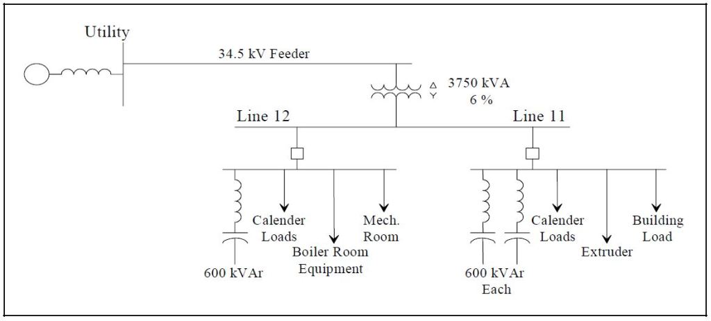
The calender lines at the new facility will be similar to existing lines at the existing facility. Therefore, measurements at the existing facility are used to estimate the power factor correction that will be needed at the new facility. Since all of the load will essentially be connected to the same 480 volt bus at the new facility, the important consideration is the total power factor for the two switchgear lines.
Measurement Results
Measurements were performed characterizing typical calender line conditions at the existing facility. There were two very important findings from these measurements:
Power Factor Calculations for the New Facility
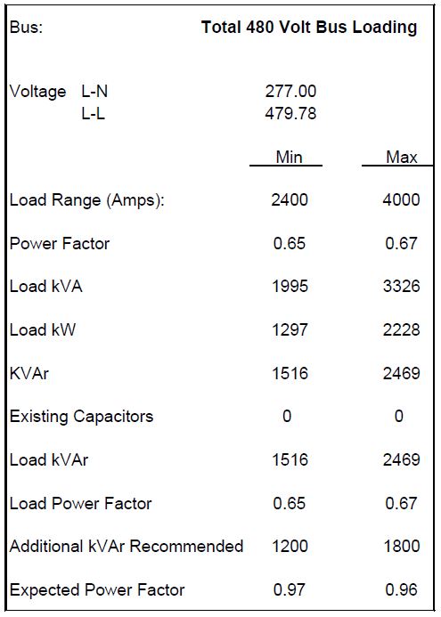
The power factor requirements for the new facility are calculated based on the total expected load. Table 1 shows the calculation of the power factor correction requirements at estimated minimum and maximum load levels. The estimated power factor of the loads is based on the measurement results. Based on these estimates of plant loading, a total compensation of 1800 kVAr should be sufficient to maintain a power factor exceeding 0.95 for all load conditions.
Table 1 – Calculation of Power Factor Correction for Total Plant Loading
For the purposes of harmonic analysis, the dc drive loads can be represented as sources of harmonic currents. The system looks stiff to these loads and the current waveform illustrated in Figure 1 is relatively independent of the voltage distortion at the drive location. This assumption of a harmonic current source permits the system response characteristics to be evaluated separately from the dc drive characteristics. The representation of the drives as harmonic current sources is shown in Figure 3.
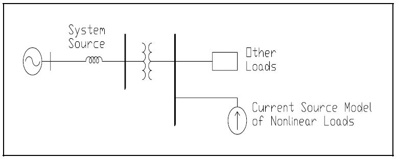
Analysis of the system response is important because the system impedance vs. frequency characteristics determine the voltage distortion that will result from the dc drive harmonic currents. A simplified version of the situation is shown in Figure 4.

If the system is infinitely strong (no impedance), there will never be any voltage distortion. It is the harmonic currents generated by the dc drives passing through the system impedance that causes voltage distortion. Filters are the means used to control the system response.
Harmonic Distortion Levels at the Existing Facility
Initial power factor correction procedures for the existing facility involved installation of capacitor banks for each calender line. One or two 600 kVAr banks were used for each line. This resulted in problems with high voltage distortion levels in the plant and also caused transient voltage magnification when the utility company switched a higher voltage transmission system capacitor bank. To prevent these problems, the 600 kVAr capacitor banks are being configured as harmonic filters rather than just capacitors. The configuration is shown in Figure 5.

The filter is tuned below the fifth harmonic. This limits the additional harmonic current that must be absorbed from the utility system and also allows for tolerances in the filter components.
The addition of a single 600 kVAr filter significantly improved voltage distortion levels at the 480 Volt bus. Figure 6 compares the voltage harmonic spectrum with and without the filter in service.

Filter Design for the New Facility
The switchgear lineups at the new facility are being configured with 1200 Amp switchgear. For this reason, the individual power factor correction steps are being limited to 600 kVAr. Based on the power factor correction estimates, two steps will be installed initially and a third step will be added in the future if it is warranted based on actual plant loading.
Each 600 kVAr step will be configured as a harmonic filter tuned to approximately 4.7 times the fundamental frequency (60 Hz). 600 volt capacitors will be used for these filters to prevent overloading due to voltage rise across the reactor and harmonics from the power system. In order to accomplish this, capacitors with a nominal rating of 900 kVAr at 600 Volts will be required. Figure 7 provides the specifications for the recommended filter configuration. The specifications are based on two filters sharing the maximum load at the new plant.

Evaluation of Current Limits in IEEE 519
The IEEE 519-1992, “Recommended Practice for Harmonic Control in Electric Power Systems”, provides recommended harmonic current limits for individual customers at the point of common coupling with the electric utility. The utility supplying the new facility has specified these harmonic current limits in the contract with the customer. Therefore, it is important to make sure that the specified harmonic filters will adequately limit the harmonic currents injected onto the utility system.
A few assumptions are required to make this evaluation. A short circuit capacity at the transformer high side of 23 MVA is assumed. This is relatively low because the plant is supplied from a long 34.5 kV feeder circuit. Worst case harmonic generation levels are assumed which do not include significant cancellation from the different drives. The IEEE 519 evaluation is based on an “average maximum demand current” defined as the average of the monthly maximum demand values for twelve months. For a new plant this must be estimated. 3000 kVA was used for this evaluation.
Figure 8 evaluates the expected current distortion levels with respect to the IEEE 519 limits for the case without compensation or harmonic filters. The limits are exceeded at almost every individual harmonic frequency and for the total demand distortion (TDD).

Figure 9 illustrates the effect of the proposed 600 kVAr filters on the expected harmonic current levels being injected onto the utility system. These values were obtained from a simulation of the system response. The limits are not exceeded at any individual frequency or for the total demand distortion. There should be no problem with the IEEE 519 limits for the proposed filter configuration.

DC Drive loads can have a low displacement power factor, resulting in a need for power factor correction. The power factor correction can be sized based on the displacement power factor of the load but all of the compensation should be installed as harmonic filters to avoid harmonic resonance problems and excessive voltage distortion levels. Filters tuned below the fifth harmonic will usually be adequate to keep voltage distortion levels below 5% and current harmonics injected onto the utility system below the levels specified in IEEE 519.
REFERENCES
T.E. Grebe, M.F. McGranaghan, and M. Samotyj, “Solving Harmonic Problems in Industrial Plants and Harmonic Mitigation Techniques for Adjustable Speed Drives,” Electrotech 92 Proceedings, Montreal, June 14-18, 1992.
T. Grebe, “Why Power Factor Correction Capacitors May Upset Adjustable Speed Drives,” Power Quality, May/June, 1991.
M.F. McGranaghan, R.M. Zavadil, G. Hensley, T. Singh, M. Samotyj, “Impact of Utility Switched Capacitors on Customer Systems – Magnification at Low Voltage Capacitors,” Presented at the 1991 IEEE T&D Show, Dallas, TX, September, 1991.
GLOSSARY AND ACRONYMS
PCC: Point of Common Coupling
SCR: Short Circuit Ratio
TDD: Total Demand Distortion
THD: Total Harmonic Distort
Published by K. B. Mohd. Umar Ansari1, Manjeet Singh2, Sandeep Kumar3
B.E (EEE), M.Tech (Electrical Power & Energy Systems), Ex- Engineer – GET, Tata Motors Pvt. Ltd., Sector 11,
Udham Singh Nagar, Pantnagar, UK, India. 1
B.Tech (EN), Ex-Electrical Engineer, Flowmore Limited, Sahibabad, Ghaziabad, U.P., India2
B.Tech (EE), M.Tech (Power Systems*), Lecturer, Department of Electrical Engg, Sri RamSwaroop Memorial
University, Lucknow, U.P., India3
Published in International Journal of Advanced Research in Electrical, Electronics and Instrumentation Engineering (A High Impact Factor , Monthly, Peer Reviewed Journal)
Website: http://www.ijareeie.com
Vol. 7 , Issue 10, October 2018
ABSTRACT: Wind power industry is developing rapidly; more and more wind farms are being connected into power systems. Integration of large scale wind farms into power systems presents some challenges that must be addressed, such as system operation and control, system stability, and power quality. This paper discuss the impact of wind turbine generation systems operation connected to power systems, describes the main power quality parameters and requirements on such generations. Furthermore, it deals with the complexities of modelling wind turbine generation systems connected to the power grid, i.e. modelling of electrical, mechanical and aerodynamic components of the wind turbine system, including the active and reactive power control. In order to analyze power quality phenomena related to wind power generation, digital computer simulation is required to solve the complex differential equations.
KEYWORDS: Wind Turbines, Wind farms, Power quality, Wind power generation, Stability, Grid code, Connection requirements
Wind turbine technology has undergone a revolution during the last century. A wind turbine is a machine for converting the kinetic energy in the wind into mechanical energy and mechanical energy is then converted into electricity. The machine which converts mechanical energy into electrical energy is called wind generator or aero generator. If the mechanical energy is used directly by machinery, such as a pump or grinding stones, the machine is called a windmill. A WECS (Wind Energy Conversion System) is a structure that transforms the kinetic energy of the incoming air stream into electrical energy. This conversion takes place in two steps, as follows. The extraction device, named wind turbine rotor turns under the wind stream action, thus harvesting a mechanical power. The rotor drives a rotating electrical machine, the generator, which outputs electrical power.
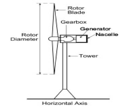

Wind turbines are classified into two general types: horizontal axis and vertical axis. A horizontal axis machine has its blades rotating on an axis parallel to the ground as shown in Fig. 1.1. A vertical axis machine has its blades rotating on an axis perpendicular to the ground as shown in Fig. 1.2. Today, the vast majority of manufactured wind turbines are horizontal axis with two or three blades.

Fig. 1.3 illustrates the major components placement in horizontal axis wind turbine.
A typical wind turbine consists of the following components:
BLADE– An important part of a wind turbine that extracts wind energy.
HUB– Blades are fixed to a hub which is a central solid part of the turbine.
GEAR BOX– Two types of gear box are used in wind turbine- Parallel shaft-It is used in small turbines, design is simple, maintenance is easy, high mass material and offset shaft. Planetary shaft- It is used in large turbines, complex design, low mass material and in line arrangements.
BRAKES-Two independent brake sets are incorporated on the rotor low speed shaft and high speed shaft The low speed shaft brake is Hydraulic operated .The high speed shaft brake is self adjusted and spring loaded.
NACELLE– The nacelle houses the generator, the gearbox, the hydraulic system and yawing mechanism.
GENERATOR– The conversion of mechanical power of wind turbine into the electrical power can be accomplished by one of the following type of the electrical machine- Synchronous machine 2. Induction machine
TOWER– Towers are made from tubular steel, concrete or steel lattice. Because wind speed is getting higher with the height, taller towers enable turbines to capture more energy and this way generates more electricity.
At the present time and in the near future, generators for wind turbines will be synchronous generators, permanent magnet synchronous generators, and induction generators, including the squirrel cage type and wound rotor type. For small to medium power wind turbines, permanent magnet generators and squirrel cage induction generators are often used because of their reliability and cost advantages. Induction generators, permanent magnet synchronous generators and wound field synchronous generators are currently used in various high power wind turbines. Interconnection apparatuses are devices to achieve power control, soft start and interconnection functions. Very often, power electronic converters are used as such devices. Most modern turbine inverters are forced commutated PWM inverters to provide a fixed voltage and fixed frequency output with a high power quality. Both voltage source voltage controlled inverters and voltage source current controlled inverters have been applied in wind turbines. For certain high power wind turbines, effective power control can be achieved with double PWM (pulse width modulation) converters which provide a bi-directional power flow between the turbine generator and the utility grid. In order to analyze wind generation compatibility in power systems four factors may be taken into account:

POWER GENERATION SYSTEM
The electrical power generation structure contains both electromagnetic and electrical subsystems. Besides the electrical generator and power electronics converter it generally contains an electrical transformer to ensure the grid voltage compatibility.
FIXED-SPEED WECS
Fixed-speed WECS operate at constant speed. That means that, regardless of the wind speed, the wind turbine rotor speed is fixed and determined by the grid frequency. Fixed-speed WECS are typically equipped with squirrel-cage induction generators (SCIG), soft starter and capacitor bank and they are connected directly to the grid, as shown in Fig.1.4.

SCIG were preferred because they are mechanically simple and have low maintenance cost. SCIG-based WECS are designed to achieve maximum power efficiency at a unique wind speed. In order to increase the power efficiency Fixed-speed WECS have the advantage of being simple, robust and reliable, with simple and inexpensive electric systems and well proven operation. On the other hand, due to the fixed-speed operation, the mechanical stress is important and full wind power is not extracted.
An evolution of the fixed-speed SCIG-based WECS are the limited variable speed WECS. They are equipped with a wound-rotor induction generator (WRIG) with variable external rotor resistance as shown in Fig. 1.5. The unique feature of this WECS is that it has a variable additional rotor resistance, controlled by power electronics. Thus, the total (internal plus external) rotor resistance is adjustable, further controlling the slip of the generator and therefore the slope of the mechanical characteristic.

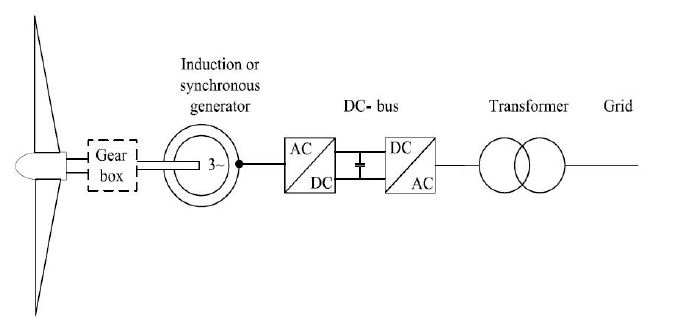
VARIABLE SPEED WECS
Variable-speed wind turbines are currently the most used WECS. The variable speed operation is possible due to the power electronic converters interface, allowing a full (or partial) decoupling from the grid. The doubly-fed-induction-generator (DFIG) based WECS shown in Fig. 1.6, also known as improved variable-speed WECS, is presently the most used by the wind turbine industry.
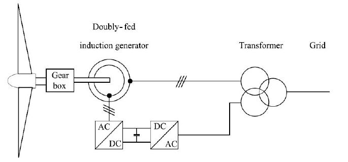
The DFIG is a WRIG with the stator windings connected directly to the three phase, constant-frequency grid and the rotor windings connected to a back-to-back (AC–AC) voltage source converter. Thus, the term “doubly-fed” comes from the fact that the stator voltage is applied from the grid and the rotor voltage is impressed by the power converter. The power electronics converter comprises of two IGBT converters, namely the rotor side and the grid side converter, connected with a direct current (DC) link. The rotor side converter controls the generator in terms of active and reactive power, while the grid side converter controls the DC-link voltage and ensures operation at a large power factor. The stator outputs power into the grid all the time. The rotor, depending on the operation point, is feeding power into the grid when the slip is negative (over synchronous operation) and it absorbs power from the grid when the slip is positive (sub-synchronous operation). In both cases, the power flow in the rotor is approximately proportional to the slip. DFIG-based WECS are highly controllable, allowing maximum power extraction over a large range of wind speeds.
The connection of wind generation to electrical power systems influences the system operation point, the load flow of real and reactive power, nodal voltages and power losses. At the same time wind power generation has various characteristics with a wide spectrum of influence which are listed below [9]:
The rising impact of wind power generation in power systems cause system operators to extend grid connection requirements in order to ensure its correct operation. We can divide grid connection requirements into two categories:
The first category represents requirements valid for every generator in the grid. These are general requirements regarding the system operation point. Some of the most important grid code requirements are:
Special requirements for wind generation were introduced to insert wind power generation in the power system without an impact on power quality or system stability.
There are two different types of requirements: requirements established by system operators and national or international standards.
The control of reactive power at the generators is used in order to keep the voltage within the required limits and avoid voltage stability problems. Wind generation should also contribute to voltage regulation in the system, the requirements either concern a certain voltage range that should be maintained at the point of connection or certain reactive power compensation that should be provided.
Until now in case of short-circuits or instability of the grid the wind parks disconnected immediately from the power system. Due to the high penetration of wind generation system operators observe a certain risk for the system stability during major disconnections. Therefore in the new regulations require that wind farms stay connected during a line voltage fault and participate in recovery from the fault.
National and international standards are applied to wind power generation regarding power quality issues for the emission of disturbances in the power system by wind generators.
In this section some possible methods of control options are discussed.

Mechanical Control of the turbine blade: As the wind speed changes the pitch of the blades or blade tip is adjusted to control the frequency of the turbine rotation.
The drawback of this method is that power in the wind is wasted and control method can be expensive and unreliable.
Load control: As the wind speed changes the electrical load is changed by rapid switching, so the turbine frequency is controlled. This method makes greater use of power in the wind because the blade pitch s kept at the optimum angle.
The advantages and disadvantages of WTIG are shown in table 1 below:
| Generator Concept | Advantages | Disadvantages |
|---|---|---|
| SCIG | Easier to design, construct and control Robust operation Low cost | Low energy yield No active/reactive power controllability High mechanical stress High losses on gear |
| PMSG | Highest energy yield Higher active/reactive power controllability Absence of brush/slip ring Low mechanical stress No copper loss on rotor | High cost of PM material Demagnetization of PM Complex construction process Higher cost on PEC Higher losses on PEC Large size |
| DFIG | High energy yield High active/reactive power controllability Lower cost on PEC Lower losses by PEC Less mechanical stress Compact size | Existence of brush/slip ring High losses on gear |
Stability support
System stability is largely associated with power system faults in a network such as tripping of transmission lines, loss of production capacity (generator unit failure) and short circuits. These failures disrupt the balance of power (active and reactive) and change the power flow. Though the capacity of the operating generators may be adequate, large voltage drops may occur suddenly. The unbalance and re-distribution of real and reactive power in the network may force the voltage to vary beyond the boundary of stability. A period of low voltage (brownout) may occur and possibly be followed by a complete loss of power (blackout).
In order to keep system stability, it is necessary to ensure that the wind turbine restores normal operation in an appropriate way and within appropriate time. This may include supporting the system voltage with reactive power compensation devices, such as interface power electronics, SVC, STATCOM and keeping the generator at appropriate speed by regulating the power etc.
The first step is to state the problem and to define a set of parameters to be analyzed giving the grid connection requirements. After that the simulation tool suitable for analyzing the stated problem and to give the requested results must be chosen. After choosing the convenient simulation software modelling of the wind turbine and power grid components should be carried out.
Wind farms consist of many relatively small generation units. Two different models could be applied to the wind farm modelling: Separated modelling of all small generation units or aggregation of these many generators to one representative wind farm model.
Wind turbines use two different models: static models and dynamic models. Static models are needed to analyze all types of steady state analysis. Usually, these models are simple and easy to create. Dynamic models are needed for various types of analysis related to system dynamics, control analysis, optimization etc.
Two different types of dynamic models are used: functional and mathematical physical models. The difference between them is that the latter one includes a detailed power electronics model. Table II compares model and analysis type. To analyze variable speed wind turbines, the following points should be considered:
As always with modelling and simulation, results should be verified by available data and measurements.
TABLE II. – Model types & analysis types
| Model | Type of analysis |
|---|---|
| Steady state static models | Analysis of voltage variation Analysis of load flow Analysis of short-circuits |
| Transient state dynamic Models functional models | Analysis of transient stability Analysis of small-signal stability Analysis of transient response Analysis of steady-state waveforms Synthesis of control Optimization |
| Transient state dynamic Models mathematical physical models (power electronics) | Analysis of start-up transient effects Analysis of load transient effects Analysis of fault operation Analysis of harmonics and sub harmonics Detailed synthesis of control Detailed optimization |
Since the penetration of wind power generation is growing system operators have an increasing interest in analyzing the impact of wind power on the connected power system. For this reason grid connection requirements are established. Integration of large scale wind power into power systems present many new challenges. This paper presents the impacts of wind power on power quality, the gird requirements for integration of wind turbines, and discusses the potential operation and control methods to meet the challenges.
REFERENCES
[1]. Sharpe, L. “Offshore generation looks set to take off”, IEE Review, Volume: 48, Issue: 3, May 2002, Page(s): 24 –25.
[2]. Grainger, B.; Thorogood, T., “Beyond the harbour wall”, IEE Review, Volume: 47, Issue: 2 , March 2001, Page(s): 13 –17.
[3]. English version of Technical Regulations TF 3.2.6, “Wind turbines connected to grids with voltage below 100 kV –Technical regulations for the properties and the control of wind turbines”, Eltra and Ekraft systems, 2004.
[4]. IEC 61400-21: Power quality requirements for wind whines. (2001).
[5]. DEFU Committee reports 111-E (2nd edition): Connection of windturbines to low and medium voltage networks 1998.
[6]. IEC 61400-12: Wind turbine generator systems. Power performance measurement techniques.
[7] http://windpower-monthly.com/windicator
[8] Blaabjerg, F., Wind Power – A Power Source Enabled by Power Electronics; 2004 CPES Power Electronics Seminar and Industry Research Review, April 18-20, Virginia Tech, Blacksburg, VA
[9] Z. Lubosny; Wind Turbine Operation in Electric Power Systems; Springer-Verlag Berlin, ISBN 3- 540 40340-X.
DOI:10.15662/IJAREEIE.2018.0710014
Published by Shuhei Kato, Miao-miao Cheng, Hideo Sumitani and Ryuichi Shimada,
Integrated Research Institute, Tokyo Institute of Technology, Japan
SUMMARY
Flywheel energy storage systems can be used as an uninterrupted power supply system because they are environmentally friendly and have high durability. The use of a simple voltage sag compensator with a low-speed heavy flywheel and a low-cost squirrel-cage induction motor/generator is proposed. First, the ability of the proposed system to maintain the load voltage at 100% when the grid is experiencing voltage sag is validated experimentally. Next, design guidelines for the flywheel stored energy are dis- cussed. Experimental verification of a 50-kW-class system is carried out, and the results show good agreement with the developed design guidelines. © 2012 Wiley Periodicals, Inc. Electr Eng Jpn, 181(1): 36–44, 2012; Published online in Wiley Online Library (wileyonlinelibrary.com). DOI 10.1002/eej.21252
Key words: flywheel; voltage sag compensator; squirrel-cage induction motor; capacitor self-excitation; design guidelines.
Voltage sag [1–3] is a phenomenon in which the grid voltage drops briefly (for about 0.1 second [4]), and in seven out of ten cases it is attributed to a lightning strike on a transmission line [5]. The frequency of occurrence of voltage sag is very high, approximately 10 to 50 times [5] that of power failures, and it causes significant losses in the form of autonomous robot failures and malfunctions in industry in general.
At present voltage sag compensators employing a parallel compensation method using an electric double layer capacitor (EDLC) [7], a NAS battery [8], or a super- conducting magnetic energy storage system (SMES) and a series compensation method known as a dynamic voltage restorer (DVR) [10], are gaining attention as voltage sag countermeasures [6]. However, in all of these semiconductor converters, harmonic filters and series transformers are required, and the equipment is complicated.
We have proposed [11, 12] a simple voltage sag compensator that can be linked directly to the grid without a semiconductor converter, that is built around a simple and inexpensive squirrel-cage induction motor with flywheel connected to the axis. It has the significant advantage of not requiring a semiconductor converter to generate a DC volt- age even though the stored energy utilization rate is low, with switching to the induction generator during induction motor sag by using capacitor self-excitation [13] in an induction motor during compensation.
In this paper we describe experiments with a simulated voltage sag (power source voltage drop) in order to confirm the effectiveness of a voltage sag compensator with a flywheel induction motor. We clarified the flywheel stored energy design guidelines for this method and tested a 50-kW-class system based on this design. The results show that the experimental results for the system agree well with the design values, confirming the effectiveness of the design method.
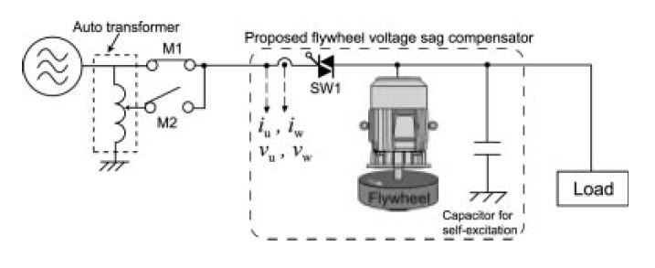
Figure 1 shows the system configuration of the volt- age sag compensator described in this paper. This is a commercial power supply system during normal operation in which the induction motor with a flywheel is connected in series to the load, and power is supplied to the load via a thyristor switch from the grid during normal operation. The actions during operation are as follows.
(1) Flywheel startup and standby operation
The induction motor starting current is suppressed and the induction motor is started up by phase control of the interconnection thyristor switch from the grid without a connection to a capacitor or load. During standby, the thyristor switch is in a conductive state at all angles, and the induction motor is in standby under virtually no load.
(2) Voltage sag occurs
When the grid voltage drops, an OFF signal is sent to SW1. When SW1 is OFF at the first current zero point after the voltage sag occurs, the induction motor automatically becomes an induction generator due to the capacitor self- excitation phenomenon, and power is supplied to the load. Because the frequency of the induction generator is lower than the grid frequency only for the “slip” portion, the load voltage vector rotates spatially at close to the slip frequency with respect to the grid voltage vector.
(3) Power restoration
When the grid voltage is restored and the voltage spatial phases on the grid side and the induction generator side (load side) agree (the voltage phase difference is zero), that is, when the voltage of the induction generator is rotated 360° in space and again matches the grid voltage, an ON signal is output to SW1. Reconnection in the state in which there is a voltage phase difference creates a disturbance in the grid and the interconnection switch faults due to the large current to the induction motor, and as a result, reconnection with the voltage phase difference near zero is always required. The process then returns to the standby state in step (1).
In the experiment, we performed a simulated voltage sag test by switching an auto-transformer tap with an electromagnetic switch. Figure 1 shows the configuration of the test system.
3.1 Content of the voltage sag experiment and voltage sag determination
The flywheel system used in the voltage sag experiment was a system in which a 200-kJ flywheel was connected to an 11-kW-class squirrel-cage induction motor. Detection of the voltage drop involved calculating the three-phase instantaneous voltage by spatial vector computations, and monitoring the power flow to SW1 as well. A voltage sag was identified when the voltage shortfall detection threshold was 80% of the rated voltage (effective value: 160 V) and the power flow was reversed. The experimental conditions were set to a resistance load of 7.2 kW, and the self-excitation capacitor was set to 750 mF (reactive power: 9.3 kvar), which was optimal for 7.2 kW. A voltage drop width of 30% (residual current of 70%) was simulated.
3.2 Results of the voltage sag experiment
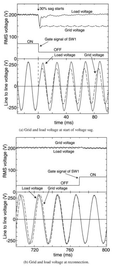
Figure 2(a) shows the results of the experiment. A voltage sag was detected at virtually the same time as the simulated voltage sag started. Because the interconnection switch is a thyristor, there is a period of approximately one-fourth of a cycle in which OFF cannot be set. We confirmed that during this period, the load voltage wave- form is chaotic, but thereafter the induction motor acts as an induction generator due to capacitor self-excitation, and a suitable voltage is generated. We then confirmed that because power is also restored in the same phase during power restoration [Fig. 2(b)], reconnection to the system is accomplished smoothly. The present voltage sag compensator does not use a semiconductor power converter to generate an AC voltage, and thus a sinusoidal voltage greater than 97% of the fundamental is generated without a filter even during compensation.
There are two points to be taken into consideration when the frequency drops and reconnection is performed during compensation in the present voltage sag compensator as described above.
(1) Reconnection to the grid cannot be performed at an arbitrary period. After the start of compensation, standby is essential until the voltage phase difference from the grid side reaches zero again.
(2) In the present method, the induction generator is reconnected directly to the grid without a semiconductor power converter. As a result, even when the instant of zero voltage phase is reached, if the frequency drops too much, excess current due to excess acceleration torque flows during reconnection, and consequently a frequency lower limit (90 to 95%) must be set. The lower limit to the frequency drop during compensation is set while taking the above two points (voltage phase zero and frequency lower limit) into consideration. The flywheel stored energy capacity leading to the same phase when the lower limit of the frequency is reached is the optimal flywheel stored energy capacity for the present voltage sag compensator. Design guidelines are given in detail below.
4.1 Derivation of the phase matching time
When the load power to be protected is Pload, the mechanical power input to the induction machine from the flywheel is Pme. The mechanical energy ΔE that the fly- wheel releases in the compensation time t is
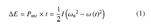
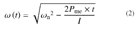
Here ωn, ω(t), and I represent the standby rotational angular velocity of the flywheel, the rotational angular velocity function after the start of compensation, and the inertial moment. The rotational angular velocity function ω(t) can be rewritten as
On the other hand, the relation between the frequency F(t) of the induction generator and the rotational angular velocity is represented by
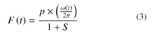
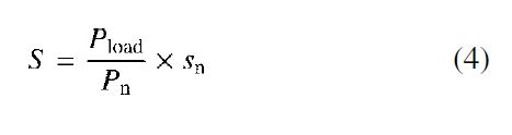
Here p is the number of pole pairs, S is the slip of the induction generator (although a negative value; S is a positive value due to inversion of the immediately preceding sign). With the slip at rated power denoted as sn and the rated power of the induction machine as Pn, we have
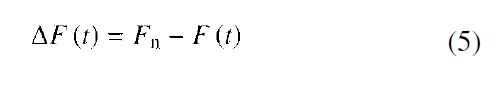
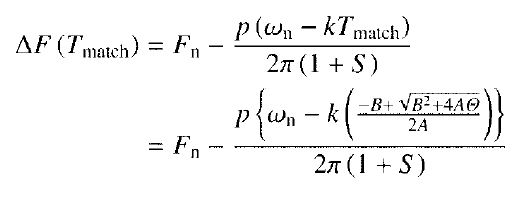
Therefore, if the rated frequency (grid frequency) is Fn, then the frequency difference ΔF(t) is
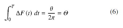
The time integral of this frequency difference is the phase angle θ, and the time t at which θ = 2π is the phase matching time Tmatch:
Here time integral (2), the rotational angular velocity function, is relatively complex. Further, Eq. (6) cannot be solved analytically in the form given. As a result, the rotational angular velocity function ω(t) is approximated linearly as
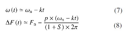
This is because when the compensation time is sufficiently small compared to the acceleration constant H = E/Pn for the rotating body, the drop in the rotational angular velocity is linear. Here k is a proportionality constant,
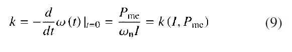
and is defined as the tangent slope of the rotational angular velocity function at t = 0. Hence, if Eq. (6) is rewritten using the voltage phase difference Θ of the grid side and the load side, the second-order constraint equation
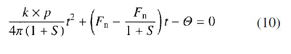
is obtained. Solving this equation, we obtain
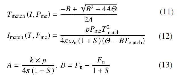
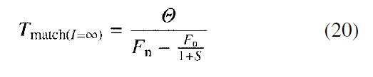
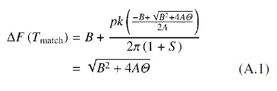
Thus, as shown in Eq. (11), after the start of compensation, the time Tmatch at which the voltage phase reaches zero again is θ = 2π, and is determined by the load power, the inertial moment, and the rated slip. Conversely, if the time Tmatch at which the same phase is reached is specified, then the required moment of inertia Imatch is determined by the time and load power, as shown in Eq. (12).
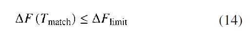
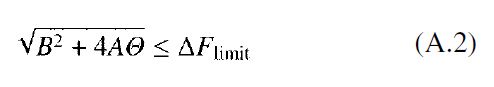
4.2 Flywheel design using the set frequency lower limit
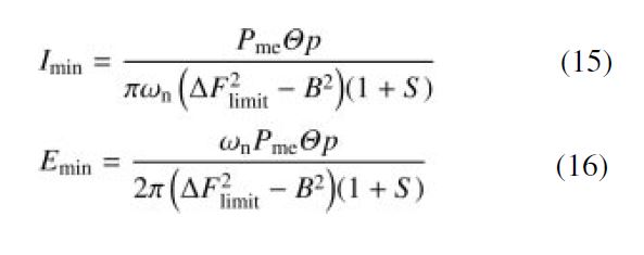
The lower limit of the frequency must be given closer consideration when designing a flywheel using the constraint equation in the previous section. That is, the frequency drop up to the time at which the voltage phase difference again reaches zero must be at least ΔFlimit. Then the constraint equation for the frequency drop is represented by
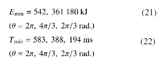
Solving this equation, we can express the necessary mini- mum inertial moment Imin and stored energy Emin by means of the following equations (see Appendix):
The time at which the same phase is reached for the stored energy Emin is
based on Eq. (11), which determines the minimum period of the compensation time.
4.3 Design of a 50-kW-class system for the voltage sag compensator
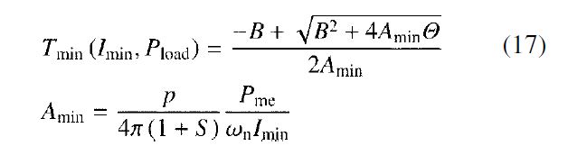
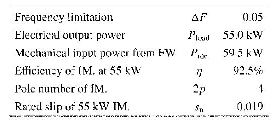
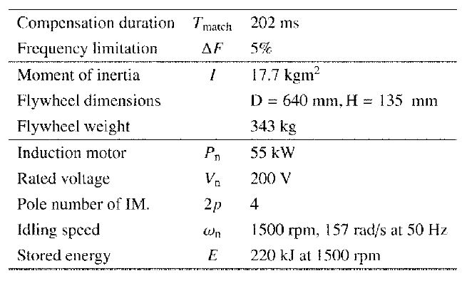
We designed a 50-kW-class system for the voltage sag compensator based on the calculations in the previous section. Table 1 gives the design conditions. Specifying a lower frequency limit 5% below the grid frequency (ΔF = 0.05), calculations were performed with the rated slip sn = 0.019 (based on a list of results for a prototype 55-kW-class induction motor) for the 55-kW-class induction motor with four poles at ωn = 1500 rpm. The necessary minimum moment of inertia to compensate a load at a load power of Pload = 55 kW (based on 92.5% efficiency of the induction machine, Pme = 59.5 kW) is found from Eqs. (15) and (17):
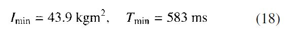
Therefore, based on Eq. (16), the necessary minimum stored energy is
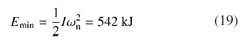
If design is performed as described above, then the compensation time when compensating a constant load at Pload = 55 kW is 583 ms
4.4 Reduction of flywheel capacity due to an improved interconnection switch
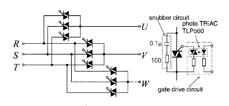
In order to restore power in the same phase when reconnecting to the grid as in the calculations in the preceding section, θ = 2π rad = 360° is assumed in Eq. (6). Thus, as shown in Fig. 3, if the interconnection switch is configured in a 9 TRIAC arrangement such as a matrix converter, then reconnection to the grid is possible in increments of θ = 2π/3 rad = 120°. In this case, the number of semiconductor switches increases, but as shown in Fig. 3, the TRIAC drive circuit has an extremely simple configuration with only a photocoupler and there is no need for an insulated power supply. Furthermore, because only three of the TRIACs have current passing through them at all times, the heat sink size (°C/W) and the constant loss in the switch do not change.
Based on this idea, Fig. 4 shows the relationship between the compensation time and the frequency difference for compensation of the rated power. The horizontal axis represents time, and the vertical axis represents the difference ΔF(t) between the grid frequency Fn and the induction generator frequency. First, if the moment of inertia of the flywheel is infinitely large, then the frequency difference is constant at Fn – Fn/(1 + S). In this case, the time to reach the same phase is I = ∞. As a result, rearranging Eq. (10) and setting k = 0, we obtain
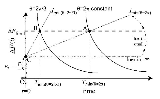
Next, when the moment of inertia is finite, the frequency difference ΔF(t) varies linearly with respect to time. If the frequency difference reaches a limit, then at the same time the moment of inertia at which the voltage phase difference changes to a constant curve with θ = 2π rad is Imin. That is, the area enclosed by the origin, point C, point A (point B when θ = 2π/3 rad), and Tmin is Θ = 1 (1/3 when θ = 2π/3 rad). The voltage phase differences q that can be selected depend on the number of phases: for three phases, there are three, namely, 2π, 4π/3, and 2π/3.
4.5 Flywheel guidelines based on an improved grid interconnection switch
Table 1. Design conditions of a 50-kW-class system
Using the improved grid interconnection switch de- scribed in the previous section, design was performed for the conditions listed in Table 1. The relationship between the compensation time and the stored energy when compensating rated power at 55 kW is shown in Fig. 5. If design is performed using region I (the dotted curve) in Fig. 5, then phase matching is reached at a given stored energy and the desired time, but the region is one in which the frequency drops below 95%. Conversely, if design is performed using region II (the dotted curve), the result is an overdesigned region in which there is still a margin for voltage drop when phase matching is reached in the desired time. Hence, the design point (optimal point) at which the frequency is 95% when phase matching is reached is the point at which the curves in Fig. 5 and the 5% frequency drop line intersect, so that
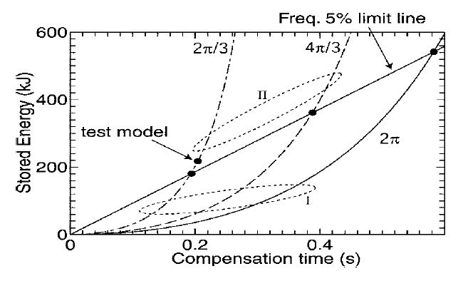
If the stored energy is greater than Emin, then the frequency drop is kept within 5% and reconnection to the grid is possible.
Based on the design guidelines in the previous section, we prototyped a 50-kW-class test system and con- firmed the validity of the design principles. The results are described below.
5.1 Specifications of the test system for the 50-kW-class voltage sag compensator
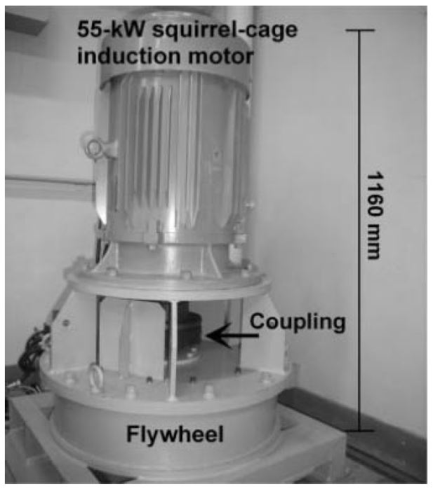
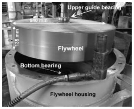
Because the majority of voltage sags are concentrated in the range of 100 to 200 ms [4], we created our test system using the test model point (reconnection to the grid at θ = 2π/3 rad) shown in Fig. 5. Table 2 lists the specifications for a 50-kW-class voltage sag compensator using the prototyped vertical-axis flywheel. Figures 6 and 7 show the external appearance.
Table 2. Test model specifications of the proposed 50-kW voltage sag compensator
5.2 Experiment to confirm the validity of the design guidelines
In order to confirm the validity of the design guide- lines for the proposed voltage sag compensator using the prototyped vertical-axis flywheel, we performed an experiment involving the opening of grid interconnection switch M1 rather than an experiment with a simulated voltage sag using the experimental configuration shown in Fig. 1. The capacitor value used for the self-excitation phenomenon was selected appropriately to the load [14], so that the induction generator produced approximately the rated volt- age Vn over a constant period during compensation. In practice, the load power often fluctuates, and countermeasures to automatically switch the capacitance as appropriate based on the fluctuations are extremely important. We performed our experiment by varying the compensation load from 10 kW to 55 kW. The total standby loss (iron loss, copper loss, wind loss, bearing loss) was approximately 1.77 kW.
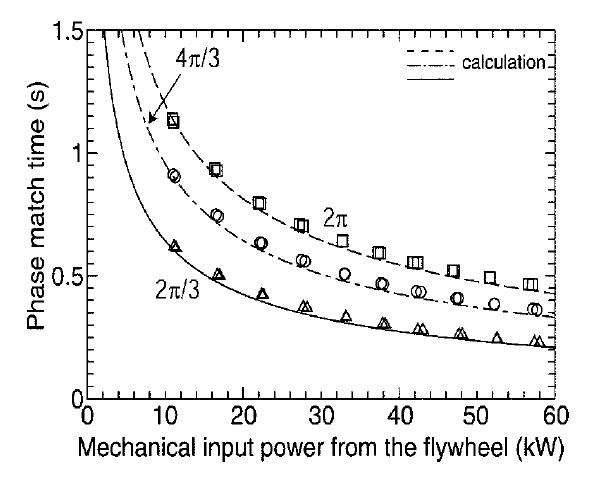
Figure 8 shows the experimentally determined matching time Tmatch for the same phase with respect to the mechanical input power Pme (the measured load power Pload divided by the efficiency of the motor with that load = the value for the mechanical load of the flywheel). For the voltage phase difference, the output q of the phase- locked loop (PLL) where the d axis voltage of the induction generator voltage is zero is calculated, and the times at which the voltage phase difference is 120°, 240°, and 360° are measured. As can be seen in the figure, the experimental results and the values calculated using Eq. (11) agree well. When the calculated value is taken as the true value, the error is positive (approximately +7% at most), and the time until the phase again matches is slightly longer.
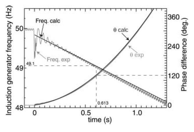
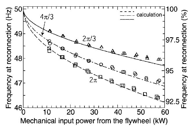
We also evaluated the induction generator frequency at phase match. Figure 9 shows the voltage phase difference and the frequency of the induction generator and the grid when the load power Pload is 10 kW. The frequency on the vertical axis was calculated from dθ/dt for the PLL. The figure confirms that the voltage phase difference expanded steadily from t = 0 s before compensation, and its time variation agreed well with the calculated values. The frequency dropped steadily, and at t = 0.613 s a voltage phase difference of 120° was obtained. The frequency at this time was 49.1 Hz. Figure 10 shows the voltage drop at phase match when varying the load power Pload as above. The experimental values for the voltage drop are more stable than the calculated values and the agreement is good. These results confirm the validity of the design guidelines in Section 4 for a system that compensates a 55-kW load for 0.22 second by reconnecting the test system to the grid at a voltage phase difference of 120°, using the grid interconnection switch in Fig. 3.
A flywheel stored energy of approximately 50 kJ is required for compensation of approximately 0.17 second when designing a 10-kW system (electrical output of 11 kW), as was the case in the previous section. If a two-pole system is used, then a voltage sag compensator with a simple horizontal axis can be created merely by having an approximately 65-kg flywheel overhang on the axis of the 11-kW-class squirrel-cage induction motor (horizontal axis). Thus, in this paper we proposed a simple voltage sag compensator using a flywheel to deal with the problem of voltage sag, and clarified the following three points.
(1) A voltage sag experiment simulating a 30% volt- age drop confirmed the effectiveness of the proposed method, which maintained approximately the rated load voltage even during reconnection immediately after the start of a voltage sag.
(2) We clarified flywheel design guidelines for our voltage sag compensator. We showed that a flywheel stored energy capacity of 180 kJ is optimal for a 50-kW system when the frequency drop during reconnection is 5%, and that the compensation time is approximately 0.20 second.
(3) We created a 50-kW-class test system (flywheel stored energy 220 kJ) based on the design guidelines. Experiments showed that the designed values and the experimental values agreed well, and demonstrated the validity of the design guidelines for a load power of 55 kW and an approximately 0.22-second compensation system.
Derivation of Eq. (15)
On the left side of Eq. (14), the conditional equation for the frequency drop during reconnection can be converted to
by using Eqs. (8) and (11). Because pωn = 2πFn, the same equation can be represented as
using Eq. (13). Therefore, the inequality in Eq. (14) can be altered to
Because both sides of the inequalities are positive, the direction of the inequality sign does not change if both sides are squared. If Eq. (A.2) is rearranged by using Eq. (13) after squaring both sides, we obtain
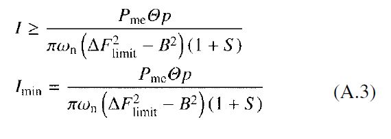
which yields Eq. (15).
AUTHORS (from left to right)

Shuhei Kato (member) completed the doctoral program in innovative energy at the Graduate School of Science and Engineering of Tokyo Institute of Technology in 2009. He is now engaged in research on energy storage using flywheels. He received a 2007 Institute of Electrical Engineers of Japan Excellent Presentation Award. He holds a D.Eng. degree.
Miao-miao Cheng (member) completed the M.E. program at Xi’an Jiaotong University in 2006 and entered the doctoral program in innovative energy at the Graduate School of Science and Engineering of Tokyo Institute of Technology. She is now engaged in research on flywheel energy storage for stabilizing distributed power source transients.
Hideo Sumitani (senior member) received a bachelor’s degree from the Department of Electrical Engineering of Tokyo Institute of Technology in 1959 and joined Toshiba, where he was engaged in the development, design, and production of AC electric motors for industry. In 1991 he joined Toshiba Techno Consulting. In 1998 he joined Tokyo Power Technical Services. In 2001 he joined Toshiba Technical Services International, and became a researcher at the Atomic Reactor Engineering Laboratory of Tokyo Institute of Technology, where he is also a visiting instructor.
Ryuichi Shimada (senior member) completed the doctoral program at the Graduate School of Tokyo Institute of Technology in 1975 and joined the Japan Atomic Energy Research Institute, where he worked on the development of the large-scale Tokamak JT-60 fusion reactor. In 1988 he became an associate professor in the Department of Electrical and Electronic Engineering in the Faculty of Engineering of Tokyo Institute of Technology. He was appointed a professor at the Atomic Reactor Engineering Laboratory there in 1990. In 2005 he became a professor at the Integrated Research Institute. He is primarily engaged in research on large-scale electric power systems, electric power engineering, electric power storage, power electronics, nuclear fusion reactor engineering, and plasma control. He has received the IEEJ Outstanding Paper Prize, Progress Prize, and Authorship Prize. He holds a D.Eng. degree.
Electrical Engineering in Japan, Vol. 181, No. 1, 2012
Translated from Denki Gakkai Ronbunshi, Vol. 129-D, No. 4, April 2011, pp. 446–452
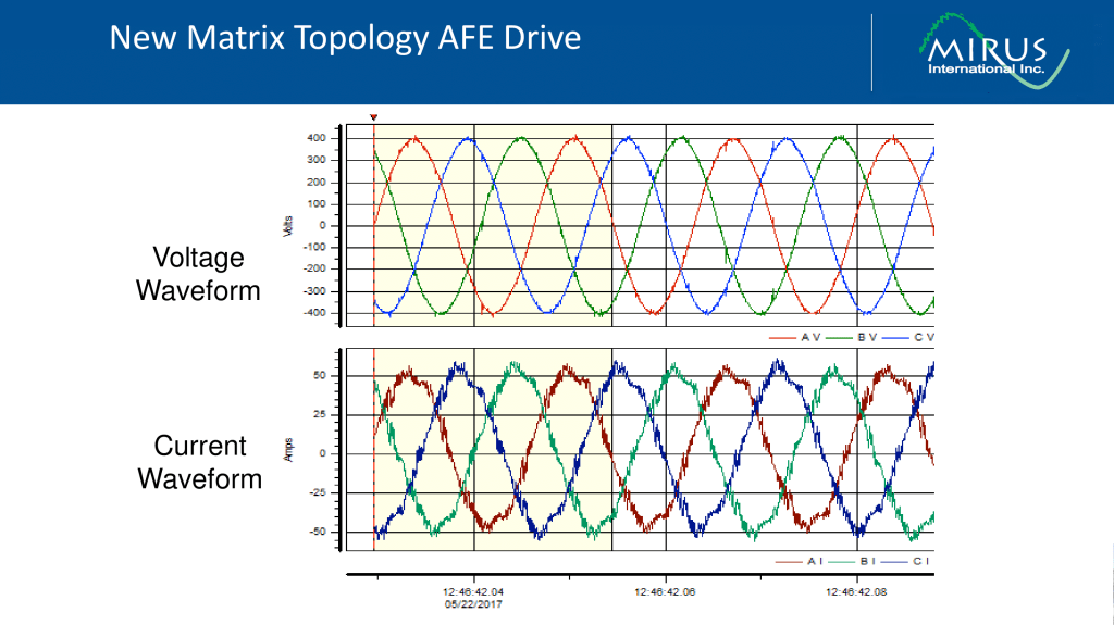
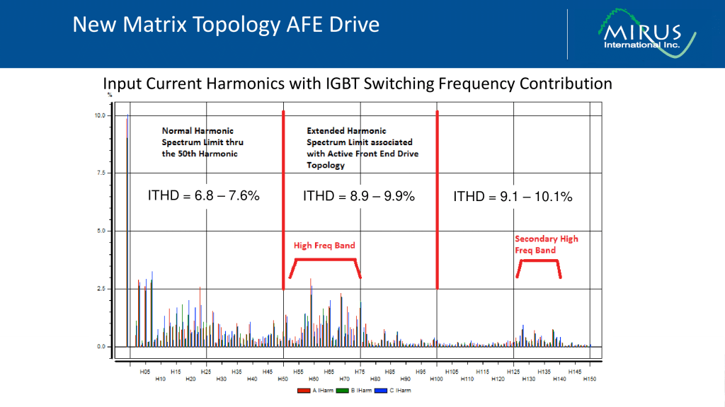
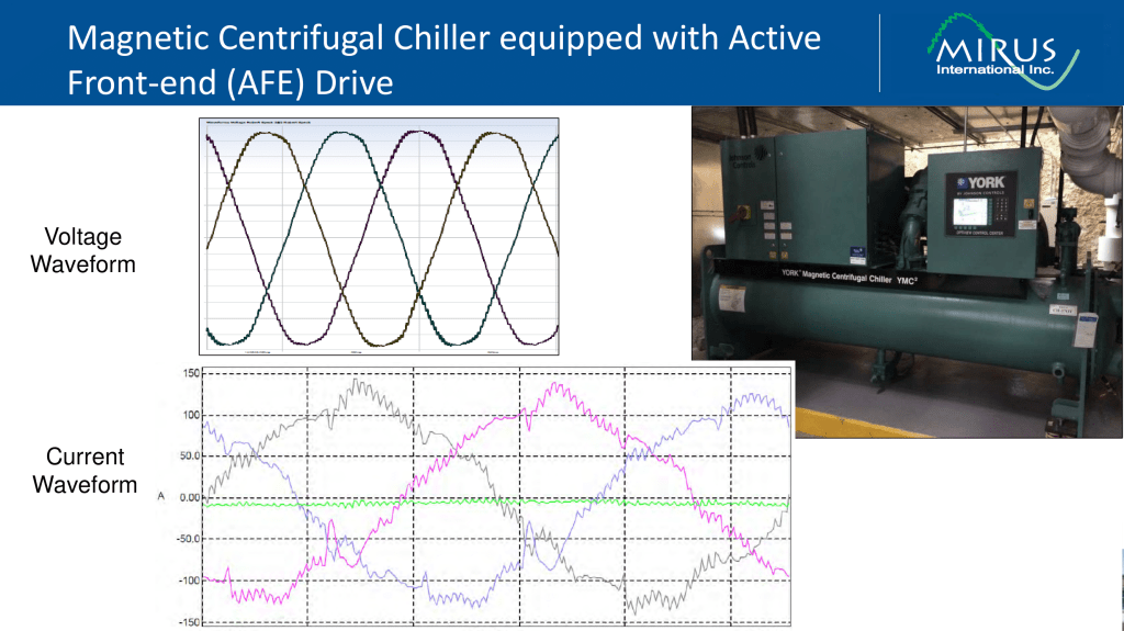
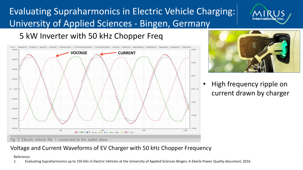
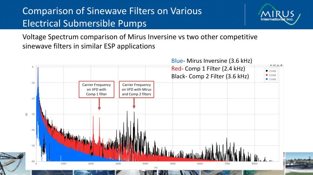
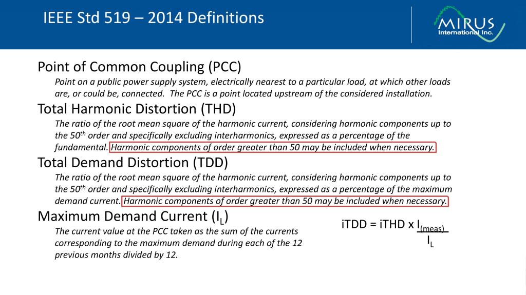
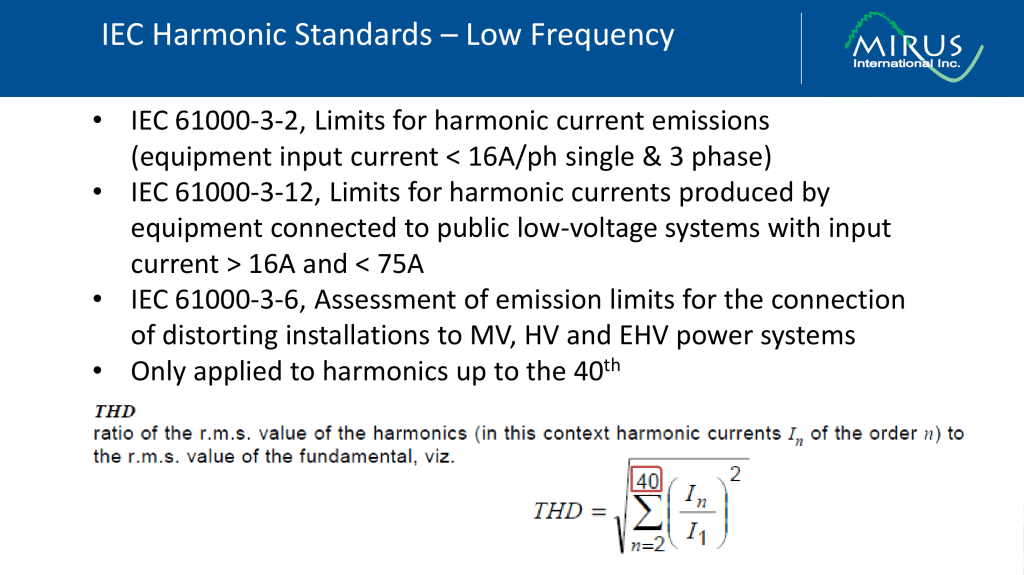
Published by Mirus International Inc., Harmonic and Energy Saving Solutions: Supraharmonics–The Next Big PQ Concern, Sept. 2020


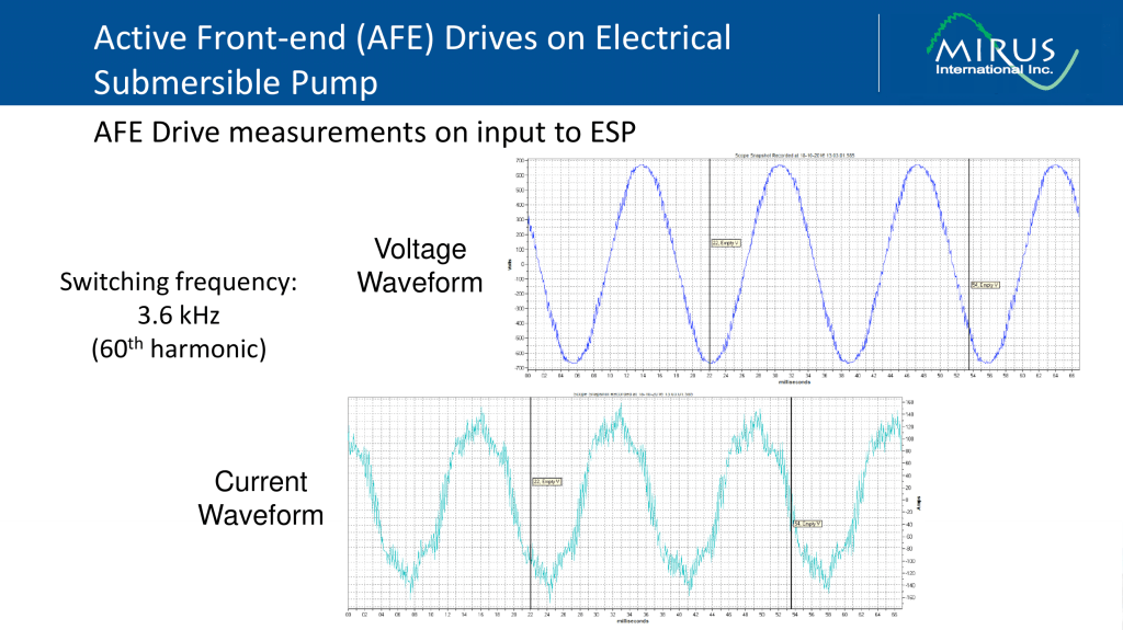


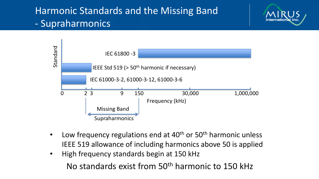


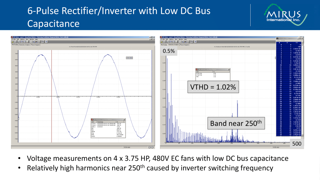
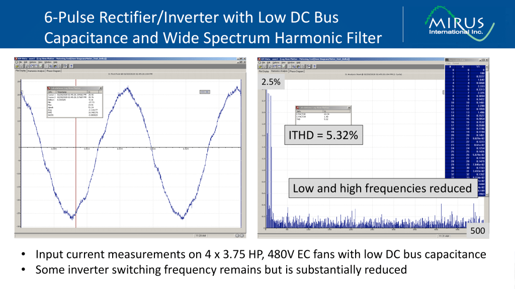
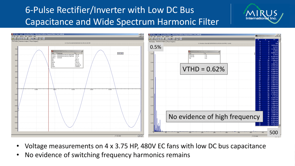


Mirus International Inc., 31 Sun Pac Blvd., Brampton, Ontario, CanadaL6S 5P6, Tel: (905) 494-1120, Fax: (905) 494-1140, Toll Free: 1-888 TO MIRUS (1-888-866-4787), Website: www.mirusinternational.com, E-mail: mirus@mirusinternational.com
Published by Electrotek Concepts, Inc., PQSoft Case Study: Power Factor Correction, Document ID: PQS0312, Date: April 16, 2003.
Abstract: Low power factor because it means that you are using the facility’s electrical system inefficiently. It can also cause equipment overloads, low voltage conditions, and greater line losses. Most importantly, low power factor can increase total demand charges and cost per kWh, resulting in higher monthly electric bills. This document provides an overview of the concept of power factor, including impacts on the electrical distribution system, effects on power quality, benefits of improvements, and estimating financial savings.
This case presents the applications of low voltage power factor correction capacitors to improve poor power factor.
A large plastics plant is paying a significant power factor penalty each month. The utility has informed the plant that correcting the overall plant power factor to 95% will eliminate the penalty.
A summary of previous utility bills is provided in Table 1.
| Month | kVA | kW | kVAr | Power Factor |
|---|---|---|---|---|
| Feb 1991 | 5880 | 4080 | 4234 | 0.694 |
| Mar 1991 | 5700 | 3900 | 4157 | 0.684 |
| etc. | ||||
| Dec 1991 | 6120 | 4200 | 4451 | 0.686 |
| etc. | ||||
| Average | 6079 | 4185 | 4408 | 0.689 |
Why Improve the Power Factor
The application of power factor correction capacitors is generally motivated by the desire to save money. Most often, this is a direct response to utility power factor penalties. However, there are several other reasons that a customer might decide to apply power factor correction capacitors.
While power factor correction alone is not a harmonic concern, it is nevertheless important to understand the relationship between capacitors and harmonic related problems.
Location for Power Factor Correction Capacitors
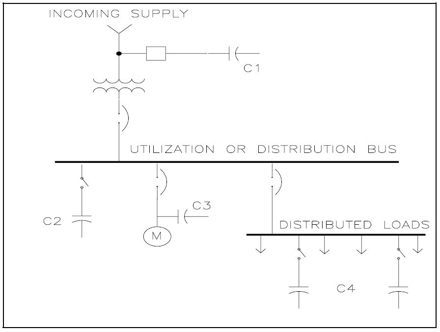
The benefits realized by installing power factor correction capacitors include the reduction of reactive power flow on the system. Therefore, for best results, power factor correction should be located as close to the load as possible. However, this may not be the most economical solution or event the best engineering solution, due to the interaction of harmonics and capacitors. Refer to Figure 1 for a oneline representation of possible placement options for power factor correction capacitors.
Often capacitors will be installed with large induction motors (C3). This allows the capacitor and motor to be switched as a unit. Large plants with extensive distribution systems often install capacitors at the primary voltage bus (C1) when utility billing encourages power factor correction. Many times however, power factor correction and harmonic distortion reduction must be accomplished with the same equipment. Location of larger harmonic filters on the distribution bus (C2) provides the required compensation and a low impedance path for harmonic currents to flow.
Evaluating the Effectiveness of a Capacitor Application
Several simple equations can be used to determine the effectiveness of power factor correction. The voltage improvement realized with the installation of capacitors is determined from:
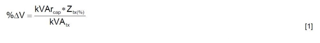
where:
%ΔV = voltage rise (percent)
kVArcap = capacitor bank rating (kVAr)
kVAtx = step-down transformer rating (kVA)
Ztx = step-down transformer impedance (percent)
Although capacitors raise a circuit’s voltage, it is rarely economical to apply them in industrial plants for that reason alone. The reduction in power system losses is determined from:
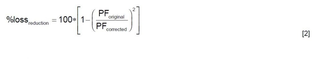
where:
%lossreduction = reduction in losses (percent)
PForiginal = original power factor (per unit)
PFcorrected = corrected power factor (per unit)
Financial return from conductor loss reduction alone is seldom sufficient to justify the installation of capacitors. It is an added benefit, especially in older plants with long distribution feeders. The optimum location of the power factor correction capacitors can be determined from a load flow analysis. However, it is important to remember that harmonic considerations are often more important than correction. Finally, the percent line current reduction can be approximated from:
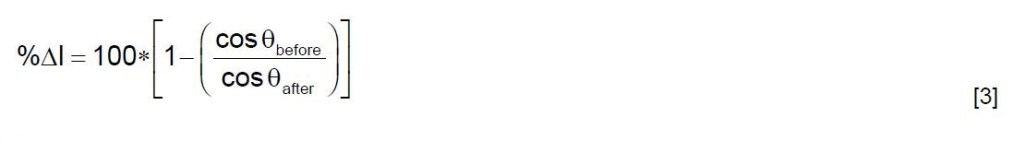
where:
%ΔV = current reduction (percent)
θbefore = power factor angle before correction (degrees)
θafter = power factor angle after correction (degrees)
Displacement Power Factor vs. True Power Factor
The traditional method of power factor correction, both on the power system and within customer facilities has been the applications of shunt capacitor banks. This is based on the fact that most loads on the system draw a lagging current (partially inductive) at the fundamental frequency. Capacitors draw a leading current at the fundamental frequency and, therefore, can compensate for the current drawn by inductive loads (motors are the most important).
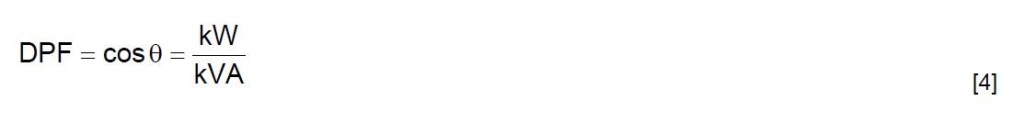
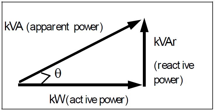
These characteristics of leading and lagging current are based on the assumption that loads on the system have linear voltage-current characteristics and that harmonic distortion of the voltage and current is not significant. With these assumptions, the power factor is equal to the displacement power factor (DPF). Calculation of the displacement power factor is completed using the traditional power factor triangle, and is summarized with the following relationship (shown in Figure 2):
Harmonic distortion in the voltage and/or current caused by nonlinear loads on the system changes the way power factor must be calculated. True power factor (TPF) is defined as the ratio of real power to the total volt-amperes in the circuit.
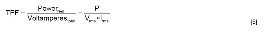
This is a measure of the efficiency with which the real power is being used. Since capacitors only provide reactive power (VArs) at the fundamental frequency, they cannot correct true power factor when there are harmonics present. In fact, capacitors can make true power factor worse by creating resonance conditions which magnify the harmonic distortion in the voltage and current.
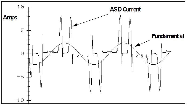
Adjustable-speed drives (ASDs) using pulse-width modulation (PWM) technology are a particularly important example of the difference between true power factor and displacement power factor. These drives use a diode bridge rectifier to convert the ac power to dc. As a result, these drives have a displacement power factor very close to unity. However, the harmonic distortion of the input current can be very high. This low true power factor cannot be improved with capacitors. Harmonic filtering is the most common way of improving power factor for this type of load.
Displacement power factor is still very important to most industrial customers because utility billing for power factor penalties is almost universally based on displacement power factor. Metering used to measure power factor is based on VAr meters that are only responsive to the fundamental frequency components of the voltage and current. Therefore, utilities do not currently penalize customers for the inefficiencies introduced by harmonics in their loads.
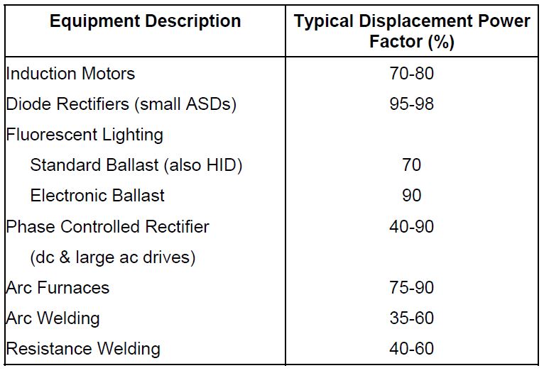
Typical Equipment Power Factors
The typical displacement power factor for individual equipment types is summarized in Table 2.
Motor Power Factor Correction Example
The following example illustrates the correction of a 500 HP induction motor with an assumed power factor of 85%. The customer desires correction to 95%. The assumption of HP = kVA is used to determine the following:
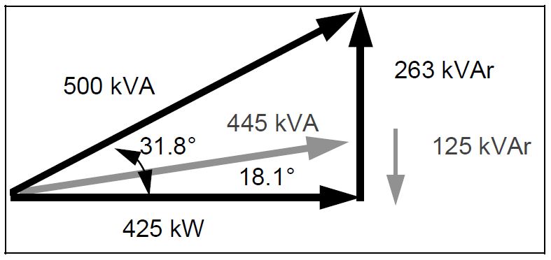
kVArrequired = (425) ∗ (tan31.8 – tan18.1) ≈ 125kVAr
where:
Original power factor angle = cos-1(0.85) = 31.8°
Desired power factor angle = cos-1(0.95) = 18.1°
Displacement vs. True Power Factor Example
The impact of harmonic distortion on power factor is illustrated using the PWM ASD current waveform shown in Figure 4.
The rms current, for the drive waveform, is determined from the following equation:
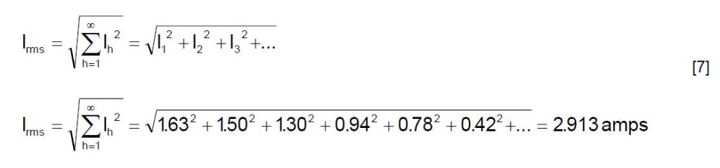
Note: Harmonic spectrum data obtained from Fast Fourier Transform (FFT) on measured waveform
The total harmonic distortion (THD), and crest factor (CF) for the current waveform are determined from:
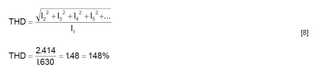
Note: Ipk obtained from measurement data.
Note: Crest Factor for a single-frequency sinusoidal wave (no distortion) is 1.412
For the drive current illustrated, it is assumed that the fundamental components of the current and voltage are in phase – displacement power factor = 100%. Actual values for waveforms of this type range from 95-98%. If we assume that the voltage distortion is negligible, the real power consumed is:
P = V1 ∗ I1 * cosθ = (480 V) (1.63 A) (1.0) = 782.4 W
The true power factor can then be determined from:
TPF = P / (Vrms ∗ Irms) = 782.4 W / (480 V * 2.913 A) = 0.56 = 56%
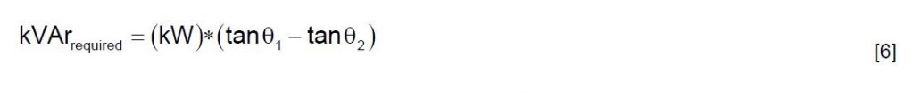
Recalling, from Table 1, the plant’s previous utility bills. The average power factor is corrected to 95% using the following method:
| Month | kVA | kW | kVAr | Power Factor |
|---|---|---|---|---|
| Feb 1991 | 5880 | 4080 | 4234 | 0.694 |
| Mar 1991 | 5700 | 3900 | 4157 | 0.684 |
| etc. | ||||
| Dec 1991 | 6120 | 4200 | 4451 | 0.686 |
| etc. | ||||
| Average | 6079 | 4185 | 4408 | 0.689 |
kVArrequired = (kW) ∗ (tanθ1 – tanθ2)
kVArrequired = (4185) ∗ (tan46.4 – tan18.1) ≈ 3000kVAr
where:
θ1 = cos-1 (4185 / 6079) = 46.4°
θ2 = cos-2 (0.95) = 18.1°
After the installation of 3000kVAr of power factor correction, the average load is:
Average kW: 4185kW
Average kVAr: 1408kVAr (4408-3000)
Average kVA 4416kVA
Average PF: 95.0%
Power factor is a measurement of how efficiently a facility uses electrical energy. A high power factor means that electrical power is being utilized effectively, while a low power factor indicates poor utilization of electric power. Low power factor can cause equipment overloads, low voltage conditions, and greater line losses. Most importantly, low power factor can increase total demand charges and cost per kWh, resulting in higher monthly electric bills.
Low power factor is generally solved by adding power factor correction capacitors to a facility’s electrical distribution system. Power factor correction capacitors supply the necessary reactive portion of power (kVAr) for inductive devices. The principle benefit is lower monthly electric bills.
REFERENCES
IEEE Recommended Practice for Electric Power Distribution for Industrial Plants (IEEE Red Book, Std 141-1986), October 1986, IEEE, ISBN: 0471856878
IEEE Recommended Practice for Industrial and Commercial Power Systems Analysis (IEEE Brown Book, Std 399-1990), December 1990, IEEE, ISBN: 1559370440
IEEE Recommended Practice for Protection and Coordination of Industrial and Commercial Power Systems, March 1988, IEEE, ISBN: 0471853925
RELATED STANDARDS
IEEE Standard 1036-1992
GLOSSARY AND ACRONYMS
ASD: Adjustable-Speed Drive
CF: Crest Factor
DPF: Displacement Power Factor
PWM: Pulse Width Modulation
THD: Total Harmonic Distortion
TPF: True Power Factor
Published by
ALEKSANDAR JANJIĆ, Department of renewable energy sources, R&D Center “Alfatec” Ltd. Bul. Nikole Tesle 63/5,18000 Niš, SERBIA, aleksandar.janjic@alfatec.rs
ZORAN P. STAJIĆ, Faculty of Electronic Engineering, University of Niš, Aleksandra Medvedeva 14, 18000 Niš, SERBIA, zoran.stajic@alfatec.rs
IVAN RADOVIĆ, ED “Elektrošumadija” Kragujevac, ED “Centar” d.o.o. Kragujevac, Slobode 7, 34000 Kragujevac, SERBIA, ivan.radovic@eskg.rs
Abstract: – The paper discusses power and especially voltage quality issues in the smart grid environment. New demands that are facing the distribution network, by introducing the concept of intelligent networks (Smart Grids), are presented. Some examples of non compliance of laws and practices in Serbia are presented as well, as the illustration of lack of strategic planning in the field. Through several case studies, a few typical problems regarding power quality, occurring in the electrical utilities in Serbia, which have to be solved in a new environment are presented. In the end, the conclusion and specific suggestions in regard with the importance of strategic planning and preparation for the customization to the expected changes are given.
Key-Words: – power quality, smart grids, power quality monitoring, harmonics, volt var control
European Smart grid concept – The EU Smart Grids Technology Platform vision and strategy for Europe’s Electricity Networks of the Future was launched in 2006 [1]. The Smart Grid vision is aiming for “new products, processes and services, improving industrial efficiency and use of cleaner energy resources, while providing a competitive edge for Europe in the global marketplace”. The Smart Grid vision is highly important as a mean for support of the EU environmental as well as economical ambitions. Many of new technologies are involved, such as renewables, electric cars, and power flow control equipment, while an increased use of digital communication and control, including smart metering and advanced grid wide area real-time monitoring, can also be expected.
Principal functionality characteristics of Smart Grids are [2, 3]:
To fulfill these requirements, the evolution of existing grids is necessary, and it includes:
However, this evolution of existing grids will confront them with new challenges regarding power quality issues. Regarding distributed generation for instance, depending on applied technology (synchronous, single or doubly fed induction machines, or inverter technology) influence on power quality will be manifested through [4]:
Based on this facts, one can conclude that voltage quality is becoming increasingly important to customers for two reasons:
a) Voltage quality levels are affected by the increased use of distributed generation and different electronic devices (inverters, battery chargers, energy saving lamps).
b) Sensitive electronic devices are strongly affected by voltage quality.
Not only for consumers, but for all stakeholders involved in new, smart grid environment, power quality deserves particular attention. Thus, potential disturbance source may be found on both, generation and consumer side. From regulator point of view, it is important to asses what should be consider in establishing a regulatory framework for voltage quality in distribution networks.
The aim of this paper is to emphasize the need of improved and enhanced power quality monitoring, taking into account new requirements and new technologies of Smart grid. Finally, actions regarding power quality cannot be treated independently, without broad strategic planning frame.
In the following Section, the need for change of actual power quality policies and the need for integrated planning of all power aspects are presented through some examples of Serbian Power Industry.
In the Section 3, new smart grid functions addressing power quality aspects are presented. Through several study cases from Serbian Electrical Utilities, the need for integrated platform including power quality is presented.
Finally, conclusions are brought regarding the change in power quality treatment in the new environment.
Until now, the main focus of quality regulation has been on the reliability and commercial dimensions of quality. In contrast, there is far less experience with the issue of voltage quality regulation, especially in integrated, multi-functional and multicommunication platform like smart grid.
The proper approach to the smart grids and all matters related to this concept, and the issue of power quality, can be of a crucial importance for the countries that will be found in the way of its application.
If serious attention is not given to strategic planning and appropriate actions for preparing the system to move to a new concept are not taken, one can easily get into a situation that much greater financial resources are spent to remedy the consequences of damage, loss coverage, or on payment of fees and penalties. The only alternative is the timely planning and implementation of actions to predict and mitigate the occurrence of such losses and to optimize the adaptation to market conditions.
Disharmony between regulatory requirements and actual network level will be explained in the case of Serbian Electric Power Industry in the last decade. First example was the question of increasing the nominal voltage in low voltage distribution systems from 380 to 400 V.
Being aware of this change, many countries have made adequate preparations so the transition did not cause adverse effects. On the other hand, Serbia did not have an adequate attitude towards this issue, so the transition to a higher voltage level was carried out without any previous preparation. As a consequence, because motors in electrical drives were not replaced with new ones, designed for rated voltage of 400 V, a large increase of reactive power consumption appeared in the whole distribution system. This is especially contributed by the fact that, with the changes of rated power, the maximal allowed voltage in distribution networks in Serbia has increased even at 440 V. The second negative consequence was much larger number of failures in electrical drives.
Another example of poor strategic planning was the lack of high level incentives for customers to reduce their reactive power consumption. Without these incentives, consumers did not have any interest to invest in reactive power reduction. The problem could have been easily resolved by introduction of an appropriate tariff system. Since this was not done, after an increase of reactive power consumption in the system, Electric Power Industry of Serbia has invested in installation of reactive power compensation units in distribution networks, with the total installed capacity of 600 MVAr.
The previous examples show that due to lack of strategic planning and appropriate actions, the huge financial resources have been spent on unnecessary delays in manufacturing processes, repair of damaged equipment, insurance premiums, coverage of unnecessary energy losses and the investments in equipment that have not been necessary. All these actions have treated only the consequences, not the real causes of the problem.
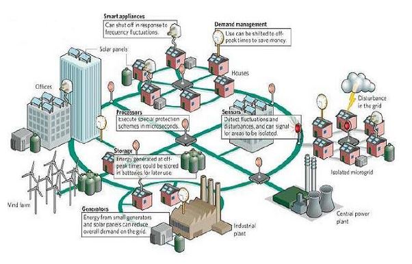
By the introduction of the smart grid concept, the focus is changed, and new information and telecommunication infrastructure is required, as presented in figure 1. Power quality monitoring has to be included in this new infrastructure as well.
The effective realization of smart grid concept is not possible without advanced distribution network automation. This automation introduces advanced distribution network operation as well, through the set of advanced distribution functions. The key aspect of electricity supply quality in a power system is the optimal application of voltage levels to all transmission and distribution networks. With significant penetration of distributed generation, the distribution network has become an active system with power flows and voltages determined by the generation as well as by the loads. Growing customer expectations and using of sophisticated electrical equipment are putting an additional responsibility upon the network operator to ensure that the delivered level and quality of supply are maintained within the parameters previously set by the regulatory bodies, while the maximal amount of distributed generation to be installed and operated is permitted at the same time. Some of innovative solution in that field are elaborated in [5, 6, 7, 8].
Integrated Volt/Var control is an important and one of the most desirable functions of a modern Distribution Automation (DA) system, as an integral part of Smart Grids. This function deals with the complexity of voltage and reactive power control in distribution systems. This complexity usually limits the capabilities of local automatic controllers which conventionally control Load Changing Transformers (LTCS) or Voltage Regulators (VRS) on the bases of local voltage measurements, and, Capacitor (CAP) banks on the bases of temperature or voltage changes.
Performing the Volt/Var control in an integrated manner provides a flat voltage profile over the feeder and at the same time minimizes the power loss in the system. In addition, a coordinated operation of VRS and CAP banks permits avoiding of an excessive and unnecessary tripping of these devices.
Centralized voltage and reactive power control is typically considered the most cost effective function of real-time DA. Rule based Centralized Capacitor Control with an objective of unity power factor has a relatively long history of real-time implementation. With development of a more reliable real-time Power Flow, the power flow based on Optimal Volt/VAr control attracts more and more attention.
Optimal Volt/VAr control allows a wider choice of objectives which can be achieved with higher mathematical accuracy. The objective of operating the distribution network within voltage and loading constraints serves as the primary objective, where other objectives – power losses, demand, etc. – serve as secondary. In addition, more and more distribution utilities are investing in remotely controlled capacitors and step voltage regulators as part of their distribution automation strategy. This offers the opportunity for periodic closed loop Volt/VAR control, which determines the optimal set of control actions and executes them immediately.
Fault Location, Isolation, and Restoration applications in a DA environment have also recently increased in importance. The trend for these applications is going towards more intelligent solutions that react to fault events and assist the operator in clearing and restoring the fault or taking action without any operator interaction at all. Fault location programs evaluate the SCADA information of breaker trip events and faults.
However, the proper introduction of these function is not possible without advanced monitoring of all important values in the power network, including the monitoring of voltage quality. In other words, power quality monitoring, together with the proper information and telecommunication techniques, is becoming the back bone of fully implemented smart grid.
A few of the case studies taken from authors experiences in Serbian power network will demonstrate the need of advanced and integrated measurement and data analysis.
3.1 Case Study 1
The first case study represents the common problem of voltage reduction in the transmission system. Due to some problem of unbalance between production and consumption, transmission network operators are commonly performing the short term (1 – 2h) voltage reduction (of the order of 5 – 10%). This reduction is leading to the short term demand reduction, but after few hours, the demand is continuing to grow, because of the „pay back effect“. Consequently, the problem is the drastic decrease of voltage quality for many customers, affected by this wide area voltage reduction.
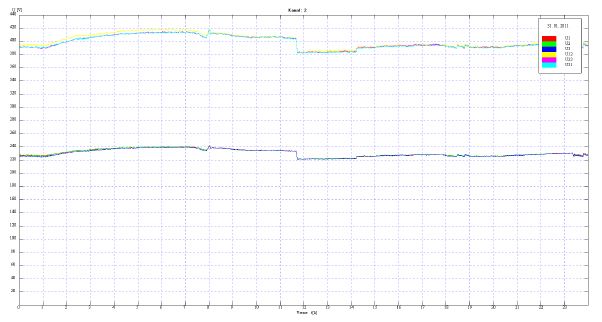
Figure 2 is representing voltages measured in one TS 10/0,4 kV, at the low voltage bus bars. The voltage magnitude decrease is of order of 10%, registered after 10 a.m. in total duration of 1 hour and 30 minutes.

The distribution company has not been warned, so the situation represented in figure 1 had as the result, many customers complaints of the low voltage in their households.
Figure 3 represents diagrams of active and reactive power from the TS 400/110 kV „Petrovac“ at one 110 kV transformer bay, which supplies, through one intermediate TS 110/35 kV „Ilićevo“ and one TS 35/10 kV „21. oktobar“, the TS 10/0.4 kV „Kadinjača“, represented in figure 2.
The measurement information system (MIS) in the TS “Kadinjača”, recorded data with 12 s time resolution. The architecture of measurement information system installed in TS 10/0,4 kV to record the parameters of voltage quality in power distribution networks is presented in figure 4.

The measurement system which measured the active and reactive power at 400/110 kV “Petrovac” recorded the data at 900 s (15 min), and forms of change shown in the diagram would not faithfully convey.

The presented example aims to demonstrate the need of measuring information system with adequately allocated measuring units, and analysis software that allows the analysis of recorded data (for instance, data recorded from other distribution utilities which are equipped with similar devices). Figures 5 and 6 show the diagrams of voltage changes in two other TS 10/0,4 kV in other areas supplied by the same TS 400/110 kV.

It is shown that without data recorded by measuring information systems and proper analysis software, many phenomena affecting the quality of voltage in electricity distribution network, when their causes are out of the site of measurement (and even outside the territory covered by the entire company for distribution) often can not be explain.
3.2 Case Study 2
Above was already stated that performing the Volt/Var control in an integrated manner provides a flat voltage profile over the feeder while minimizing the power loss on the system. In addition, a coordinated operation of VRS and CAP banks permits avoiding of an excessive and unnecessary tripping of these devices. The simplified layout of one distribution feeder is represented in figure 7.

The load connected to the main bus bars, presented in figure 7, represents one wood processing facility. Voltage variation is represented in figure 8. The problem in this particular case was the excessive operation of On Line Tap Changer (OLTC) in distribution transformer station. Only after installation of power quality measurement device and, what is more important, introduction of these measurement in the central data warehouse, the problem is solved by proper settings of OLTC in supply transformer station.

The same problem was registered in another TS 110/10 kV station, which supplied one TS 10/0,4 kV with voltage variations represented on figure 9.

Only after detection of sources of voltage variations at the lower level, the proper setting of OLTC in supplying station were possible.
3.3 Case Study 3
The final case study is dedicated to the problem of harmonics. The following is the example of electricity customer who injected into the network a large content of higher harmonics and caused unauthorized voltage drops of other electricity customers in the region. Figure 10 represents the active, reactive, and apparent powers of the consumer.


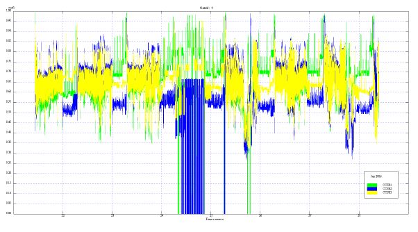
Fig. 11 presents the high level of THDu (greater than 12%), while Figure 12 presents the corresponding power factor. Checking the technical requirements for the connection, the conclusion was that are connected to the network without their fulfillment.
The paper points out that the problem of monitoring power quality parameters in Serbia should be given far more serious attention in order to adopt laws and standards in the EU, and to fulfill requirements regarding EU Smart Grid technology platform.
It is shown that solutions for problems described above should not be sought independently but as part of the development concept of intelligent networks (smart grids).
Moreover, power quality problem can be one of additional “driving factors” for the implementation of Intelligent network in Serbia.
Finally, it is shown that only the elaboration of an integrated information platform is required for resolving of power quality issues in a satisfactory manner.
Acknowledgement: The work presented here was supported by the Serbian Ministry of Education and Science (project III44006).
References:
[1] Toward Smart Power Networks, Lessons learned from European research FP5 projects, European Commission, 2005.
[2] Strategic Research Agenda for Europe Electricity Networks of the Future European Technology Platform, European Commission, April 2007.
[3] Strategic Deployment Document for Europe Electricity Networks of the Future European Technology Platform, European Commission, April 2010.
[4] T. Degner, J. Schmidt, P. Strauss, Dispower, Distributed Generation with High Penetration of Renewable Energy Sources, Final Public Report, iSET, Kassel, 2005.
[5] M. H. J. Bollen, J. Zhong et all. Power Quality aspects of Smart Grids International Conference on Renewable Energies and Power Quality (ICREPQ’10) Granada (Spain), 23th to 25th March, 2010.
[6] H. Spaack et all. Intelligent Transformer Substations in Modern Medium Voltage Networks as Part of “Smart Grid” 7th Mediterranean Conference and Exhibition on Power Generation, Transmission, Distribution and Energy Conversion7-10 November 2010, Agia Napa, Cyprus (Paper No. MED10/240).
[7] J. Kester et all. A smart MV/LV station that improves power quality, reliability and substation load profile, 20th International Conference on Electricity Distribution Prague, 8-11 June 2009.
[8] J. Heckel, Smart substation and feeder automation for a smart distribution grid, 20th International Conference on Electricity Distribution Prague, 8-11 June 2009.
ISBN: 978-1-61804-023-7
Source URL: http://media.alfatec.rs/2011/10/Power-Quality-in-Smart-Grid-Environment-Serbian-Case-Studies.pdf
Published by Electrotek Concepts, Inc., PQSoft Case Study: General Reference – Power Factor Correction, Document ID: PQS0311, Date: April 16, 2003.
Abstract: Simply stated, power factor is a measurement of how efficiently a facility uses electrical energy. A high power factor means that electrical power is being utilized effectively, while a low power factor indicates poor utilization of electric power.
Low power factor because it means that you are using the facility’s electrical system inefficiently. It can also cause equipment overloads, low voltage conditions, and greater line losses. Most importantly, low power factor can increase total demand charges and cost per kWh, resulting in higher monthly electric bills. This document provides an overview of the concept of power factor, including impacts on the electrical distribution system, effects on power quality, benefits of improvements, and estimating financial savings.
A large number of customer loads in a modern electrical system are inductive, which means that they require an electromagnetic field to operate. Inductive loads, such as motors, require two kinds of electric power:
Power factor involves the relationship between these two types of power. Active Power is measured in kilowatts (kW) and Reactive Power is measured in kilovolt-amperes-reactive (kVAr). Active power and reactive power together make up Apparent Power, which is measured in kilovolt-amperes (kVA). This relationship is often illustrated using the familiar “power” triangle (Figure 1):

Power factor measures how effectively electrical power is being used. Power factor is the ratio between active power (kW) and apparent power (kVA). Active power does work and reactive power produces an electromagnetic field for inductive loads. Using the values in the power triangle example, the facility is operating at 400 kW (Active Power) with an 80% power factor, resulting in a total load of 500 kVA.
Low power factor means that you are using a facility’s electrical system inefficiently. It can also cause equipment overloads, low voltage conditions, and greater line losses. Most importantly, low power factor can increase total demand charges and cost per kWh, resulting in higher monthly electric bills.
Effect of Load on Power Factor
Lightly-loaded or varying-load inductive equipment such as HVAC systems, induction furnaces, molding equipment, presses, etc. One of the worst offenders is a lightly loaded induction motor. Examples of equipment with:
Benefits of Improving Power Factor
The principle benefit is lower monthly electric bills. Additional benefits include:
Most Common Method for Improving Power Factor?
Low power factor is generally solved by adding power factor correction capacitors to a facility’s electrical distribution system. Power factor correction capacitors supply the necessary reactive portion of power (kVAr) for inductive devices. By supplying its own source of reactive power, a facility frees the utility from having to supply it. This generally results in a reduction in total customer demand and energy charges.
Power factor correction capacitors are rated in electrical terms called “VArs”. One VAr is equivalent to one volt-amp of reactor power. Since reactive power is generally measured in thousands of vars, the letter “k” (abbreviation for kilo) proceeds the Var creating the more familiar “kVAr” term. Therefore, a capacitor kVAr rating indicates how much reactive power the capacitor will supply.
The amount of power factor correction that is required to correct a facility to a target power factor level is the difference between the amount of kVAr in the uncorrected system (required by loads) and the amount of kVAr in the corrected system. A capacitor application is illustrated in the following power triangle (Figure 2):
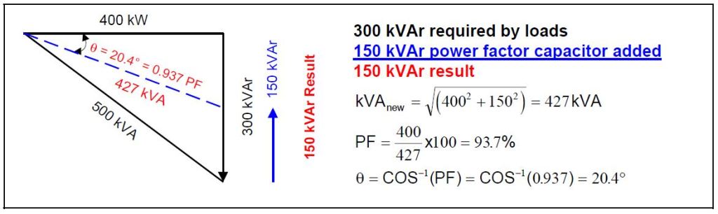
The location that provides the maximum benefits of power factor correction is at the load. Capacitors work from the point of installation back to the generating source. However, individual load (e.g. motor – shown in Figure 3) correction is not always practical and ongoing maintenance may become an issue as well. Sometimes it is more effective to connect larger capacitor banks to the main distribution bus, or to install automatic systems at the incoming service in conjunction with fixed capacitors at distributed loads.
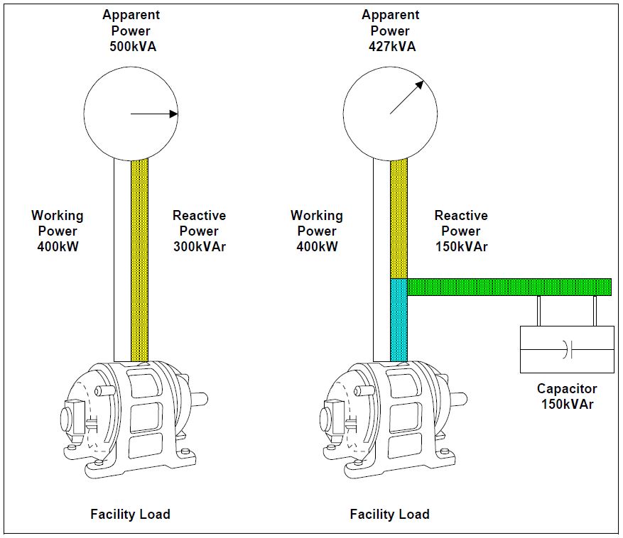
A properly designed capacitor application should not have an adverse affect on equipment or power quality. However, despite the significant benefits that can be realized using power factor correction capacitors, there are a number of power quality-related concerns that should be considered if you install capacitors. Potential problems include increased harmonic distortion and transient overvoltages.
Harmonic Issues
Harmonic distortion on power systems can best be described as noise that distorts the sinusoidal wave shape. Harmonics are caused by nonlinear loads (e.g. ASDs, compact fluorescent lighting, induction furnaces, etc.) connected to the power system. These loads draw nonsinusoidal currents (on a 60 Hz system, the 5th harmonic is equal to 300 Hz), which in turn react with the system impedance to produce voltage distortion. Generally, the harmonic impedances are low enough that excessive distortion levels do not occur. However, power factor correction capacitors can significantly alter this impedance and create what is known as a “resonance” condition. High voltage distortion can occur if the resonant frequency is near one of the harmonic currents produced by the nonlinear loads. A method for estimating the resonance point (hresonance) is shown in the following example:

Indications that a harmonic resonance exists include device overheating, frequent circuit breaker tripping, unexplained fuse operation, capacitor failures, and electronic equipment malfunction. Ways to avoid excessive distortion levels include altering (or moving) the capacitor size to avoid a harmful resonance point (e.g. 5th, 7th), altering the size (or moving) of the nonlinear load(s), or adding reactors to the power factor correction capacitors to configure them as harmonic filters.
Harmonic Filter Applications
In general, both harmonic problems and switching transient problems can be solved by configuring power factor correction capacitors as a “tuned bank”. This involves adding a series reactor (Xf) to the capacitor bank to form a tuned circuit (resulting in low impedance at a specific frequency).
It is common to tune the filter below the 5th harmonic (e.g. 4.7th) for most industrial facilities. It is important to note that the addition of a series reactor results in a voltage rise on the capacitor, which often means that capacitors with a higher voltage rating are required. Figure 4 illustrates a tuned filter bank using 300 kVAr capacitors rated 600 volts.

Transient Overvoltage Issues
Transient overvoltages can be caused by a number of power system switching events, however, utility capacitor switching often receives special attention due to the impact on customer equipment. Each time a utility switches a capacitor bank a transient overvoltage occurs. Generally, these overvoltages are low enough that they do not affect the customer’s system. However, high overvoltages can occur when customers have power factor correction capacitors. This phenomenon is often referred to as “voltage magnification”. Magnification occurs when the transient oscillation initiated by the utility capacitor switching excites a resonance (refer to previous definition) formed by the step-down transformer and low voltage power factor correction capacitors. Magnified overvoltages can be quite severe and the energy associated with these events can be damaging to power electronic equipment and surge protective devices (e.g. transient voltage surge suppressor – TVSS). ASDs have been found to be especially susceptible to these transients and nuisance tripping can result even when overvoltage levels are not severe.
Ways to avoid excessive voltage levels due to utility capacitor switching include altering (or moving) the capacitor size to avoid a harmful resonance point, adding high-energy low-voltage arresters (metal-oxide varistors – MOVs), or adding reactors to power factor correction capacitors to configure them as harmonic filters. The probability of nuisance tripping of ASDs can be significantly reduced by adding reactors (also known as “chokes”) to the drives.
Before investing in power factor correction capacitors, it is prudent to have the electrical system carefully analyzed to avoid potential problems with excessive transient voltages and harmonic distortion levels.
A monthly electric bill will include an additional surcharge if the rate schedule has a “power factor penalty” and the power factor is below a specific level (such as 95%). This penalty can be reduced or completely eliminated with the proper application of power factor correction capacitors. The savings realized needs to be weighed against the equipment costs to determine if the payback period is acceptable. Payback times can vary significantly due to wide range of low voltage capacitor costs (e.g. approximately $15/kVAr for fixed capacitors to $75/kVAr for adjustable filter banks).
Example Illustrating Capacitor Sizing and Payback Estimation:
Consider the following example data. Please note that this example is provided to illustrate one possible method for determining a power factor correction capacitor size and payback period. You will need to utilize your billing and rate schedule data for an accurate calculation
Example Data:
Energy Rate: $0.05/kWh
Demand Charge: $9.00/kW
Month: June
Number of Days: 30
Energy Use: 325000kWh
Demand: 800kW
Power Factor: 80%
Assumed Low Voltage Power Factor Correction Capacitor Cost: $20/kVAr
Step 1:
Determine Energy and Demand Components of the Monthly Bill:
Energy Use (kWh) * Energy Rate ($/kWh)
325,000 kWh * $0.05/kWh = $16,250
Demand (kW) * Demand Charge ($/kW)
800 kW * $9.00/kW = $7,200
Total Energy and Demand Components = $23,450
Step 2:
Determine Monthly Power Factor Penalty:
$(Total Energy and Demand Components) * (95 – Power Factor) * 0.0025
$23,450 * (95 – 80) * 0.0025 = $879
Step 3:
Determine Average Active Load (kW):
Energy Use (kWh) / (Number of Days * 24hours/day)
325,000 kWh / (30 * 24) = 451 kW
Step 4:
Determine Capacitor Rating to Correct Power Factor to 95%:
kVAr95% = (Average Active Load) * [TAN(COS-1(Power Factor)) – TAN(COS-1(0.95))]
451 kW * [TAN(COS-1(0.80)) – TAN(COS-1(0.95))]
190 kVAr (will purchase a 200 kVAr, 480 volt capacitor bank)
Step 5:
Estimate Equipment and Installation Cost:
Capacitor Bank Cost = 200 kVAr * $20/kVAr = $4,000
Estimated Installation Cost = $1,000
Total Cost = $5,000
Step 6:
Determine Payback Period:
Payback (in months) = Total Cost / Monthly Power Factor Penalty
$5,000 / $879 = 5.7 months
Note that this analysis only illustrates a simple payback and does not include operating and maintenance costs (generally low for low-voltage fixed capacitor banks), the cost of capital, or interest rates.
Power factor is a measurement of how efficiently a facility uses electrical energy. A high power factor means that electrical power is being utilized effectively, while a low power factor indicates poor utilization of electric power.
Low power factor can cause equipment overloads, low voltage conditions, and greater line losses. Most importantly, low power factor can increase total demand charges and cost per kWh, resulting in higher monthly electric bills.
Low power factor is generally solved by adding power factor correction capacitors to a facility’s electrical distribution system. Power factor correction capacitors supply the necessary reactive portion of power (kVAr) for inductive devices. The principle benefit is lower monthly electric bills.
REFERENCES
IEEE Recommended Practice for Electric Power Distribution for Industrial Plants (IEEE Red Book, Std 141-1986), October 1986, IEEE, ISBN: 0471856878
IEEE Recommended Practice for Industrial and Commercial Power Systems Analysis (IEEE Brown Book, Std 399-1990), December 1990, IEEE, ISBN: 1559370440
IEEE Recommended Practice for Protection and Coordination of Industrial and Commercial Power Systems, March 1988, IEEE, ISBN: 0471853925
Industrial and Commercial Power Systems Handbook, F. S. Prabhakara, Robert L. Smith, Ray P. Stratford, November 1995, McGraw Hill Text, ISBN: 0070506248
RELATED STANDARDS
IEEE Standard 519-1992
IEEE Standard 18-1992
IEEE Standard 1036-1992
GLOSSARY AND ACRONYMS
ASD: Adjustable-Speed Drive
HVAC: High-Voltage Air Conditioning
MOV: Metal Oxide Varistor
PF: Power Factor
PWM: Pulse Width Modulation
TVSS: Transient Voltage Surge Suppressors
Published by World Nuclear News (WNN), 24th February 2022.
Website: world-nuclear-news.org
With the attention of the world focused on events in Ukraine, one of the questions people are asking is about the country’s nuclear power industry. Here is a brief overview.
Ukraine is heavily dependent on nuclear energy, with 15 reactors generating about half of its electricity. All its current reactors are Russian-designed VVER types.
Nuclear development started in 1970, when Ukraine was part of what was then the Soviet Union, with the construction of the Chernobyl power plant. The first unit was commissioned in 1977 with unit 4 coming online in 1983. Following the accident in 1986, units 5 and 6 were cancelled in 1989.
The industry remained relatively stable during the years when the country became independent of the former Soviet Union. At the end of 1995 Zaporozhe 6 was connected to the grid making Zaporozhe the largest nuclear power station in Europe, with a net capacity of 5700 MWe. (The second largest station operating is Gravelines, near Dunkerque in France, with a net capacity of 5460 MWe.)
In August and October 2004 Khmelnitski 2 and Rovno 4 respectively were connected to the grid, bringing their long and interrupted construction to an end and adding 1900 MWe to replace that lost by closure of Chernobyl units 1 and 3 in 1996 and 2000 respectively.
The original design lifetime of the Russian reactors was 30 years, but work has taken place to allow a series of lifetime extensions.
In September 2021 the Ukrainian state-owned nuclear power firm Energoatom signed an agreement with the US-based firm Westinghouse to build four AP1000 reactors at established sites in the country. Since then Energoatom has outlined plans for further reactors – including exploring the possibility of deploying small modular reactors from US firm NuScale – as part of its goal of 24GWe of nuclear capacity by 2040.
Ukraine has access to two fuel suppliers: Russia’s TVEL and Westinghouse. Most fuel in Ukraine’s reactors is manufactured by TVEL, but the country has had an ongoing project in recent years to diversify its fuel sources
As of mid-2021, six of Ukraine’s 15 reactors were operating using fuel manufactured by Westinghouse, fabricated at its plant in Västerås in Sweden.
Earlier this month Energoatom’s CEO Petro Kotin said that: “According to the protocol, the plants will not work in case, for example, of bombing attack. In such a case, the plant is shut down and unloaded until the threat is eliminated.
“In the event of loss of the external power supply at the nuclear power plant, the autonomous power supply system starts working by means of powerful diesel generators. Ukrainian nuclear power plants are ready for such a mode of operation: the stock of diesel fuel located at nuclear power plants significantly exceeds the established standards.
“In addition, Ukrainian power units are ready even for an aircraft crash, because the containment and the reactor vessel designed to withstand corresponding risks.”
He added that two years’ worth of nuclear fuel had been stockpiled in case of interruption of supply.
The State Nuclear Regulatory Inspectorate of Ukraine has said that all four of the country’s nuclear power plants have been operating normally, with nine out of the 15 units connected to the grid as of Monday 28 February.
Ukraine’s nuclear power company Energoatom issued a statement on Tuesday 1 March saying that all the power plants were continuing to operate normally, and said its CEO Petro Kotin had asked the International Atomic Energy Agency (IAEA) to intervene to help keep the area around nuclear power plants free from military action.
The Russian Ministry of Defence’s spokesman Major General Igor Konashenkov was quoted by Russian media as saying, on the morning of 28 February, that Russian forces “have complete control and are protecting the territory” around the Zaporozhe plant, with its staff “working to maintain the facility and control the nuclear environment”.
In its update on 28 February the IAEA said that it had been told that Russian forces were “operational near the site but had not entered” Zaporozhe (also known as Zaporizhzhia) nuclear power plant in eastern Ukraine at that time.
The IAEA statement also said that Ukraine had informed them the previous week that “Russian forces had taken control of the facilities of the State Specialised Enterprise Chernobyl NPP, located within the Exclusion Zone set up after the 1986 accident. The regulator said that the shift supervisor at the site had not been replaced since 24 February but that he continued to perform his duties.
“SNRIU also provided radiation readings from the site which the IAEA assessed as low and in line with near background levels.”
The condition of Chernobyl nuclear facilities and other facilities was unchanged, it said.
IAEA Director General Rafael Mariano Grossi said the IAEA was monitoring developments in Ukraine “very closely and with grave concern” and with a special focus on the safety and security of its nuclear power plants and other nuclear-related facilities.
He stressed that the IAEA General Conference adopted a decision in 2009 that “any armed attack on and threat against nuclear facilities devoted to peaceful purposes constitutes a violation of the principles of the United Nations Charter, international law and the Statute of the Agency”.
Researched and written by World Nuclear News
Source URL: https://www.world-nuclear-news.org/Articles/A-guide-Nuclear-power-in-Ukraine
Published by Pacific Crest Transformers, 300 West Antelope Road – Medford, Oregon 97503 Tel : (541) 826 – 2113 Fax : (541) 826 – 8847. March, 2015.
Transformers serving heavy nonlinear loads are subject to increased winding temperatures due to the harmonic currents generated by those loads. This overheating can result in a shortened service life for the transformer. For example, operating a transformer at 10 degrees C above its insulation rated class will cause approximately a 50% reduction in the life of the transformer. If the over temperature gets high enough or lasts long enough, the insulation with fail which in turn will result in a transformer failure. K-factor rated transformers are designed to compensate for the presence of harmonic loading thereby preventing excess heating.
The definition for the K-factor as provided by the IEE Std. C57.110-2008 (IEEE Recommended Practice for Establishing Transformer Capacity When Supplying Nonsinusoidal Load Currents) states:
“A rating optionally applied to a transformer indicating its suitability for use with loads that draw non-sinusoidal currents.

where
Ih(pu) = the rms current at harmonic “h” (per unit of rated rms load current);
h = the harmonic order.”
Confused? – The object of this paper is to demystify the subject thereby providing a basic understanding as to the impact of K-factor on transformer design and operation.
Although transformers are inherently very efficient, there are losses associated with their design and loading. These losses are made up of core, winding (I2R), and eddy currents. Although core loss and winding loss values are largely constant and directly dependent on the quality and amount of material used, eddy currents can vary depending on load profiles.
In a transformer, the primary windings induce voltage in the secondary windings through an expanding and contracting magnetic field. Eddy currents are stray currents of electricity that are created by induction in conductors. These counter-electromotive forces (emf) are induced in opposition to the original field thereby creating opposition to current flow (resistance) which translates to losses.
Eddy current losses are expressed as a percentage of the transformer’s normal winding (I2R) as determined by Ohms law. They are a phenomena that increase in severity as the frequency of the current increases.
In an electrical power system, harmonics are current and voltage with frequencies that are integer multiples of the fundamental power frequency. That is, in a power system with a fundamental frequency of 60Hz, the second harmonic is 120Hz, the third harmonic is 180Hz, and so on. Harmonics have no useful purpose, yet contribute to losses and lower system efficiency. Harmonics return over the neutral and are dissipated as heat in connecting cables and transformers. These frequencies are referred to as non-sinusoidal loads. The presence of non-sinusoidal harmonic content in the current waveform will have the effect of increasing eddy current losses in the transformer leading to “harmonic distortion” of the fundamental power frequency waveform.
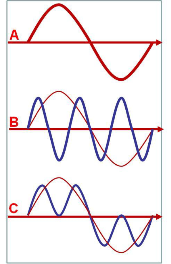
In the image to the right “A” depicts a single 60Hz cycle waveform (fundamental power frequency). “B” represents a 3rd harmonic (180Hz) waveform. The resultant waveform as shown in “C” provides an example as to the impact that the harmonic load may have on the fundamental waveform. Although the example depicts an unlikely 3rd harmonic magnitude, it provides a graphic depiction as to the impact that non-sinusoidal content can have on the fundamental waveform. The magnitude of the distortion is dependent on the number and magnitude of the total harmonic load profile.
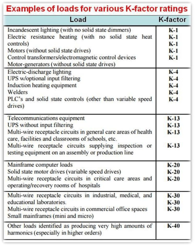
The table to the right provides an example of environments in which various K-factor rated transformers would be used. A transformer “K-factor” rating conveys its ability to manage varying degrees of nonlinear loads without exceeding the rated temperature rise limits. For any given nonlinear load, if the harmonic current components are known, the K-factor can be calculated and compared to the transformer’s nameplate K-factor. As long as the load K-factor is equal to or less than the transformer’s rated K-factor, the transformer does not need to be de-rated. The higher the K-factor, the more non-linear loads the transformer can handle. The actual formula to determine K-factor takes into account the frequency and current intensity of each individual harmonic.
The identification, measurement, and determination of the presence of non-sinusoidal frequency loads is essential in determining the impact on a transformer load. ANSI/IEEE C57.110, is the guide for determining the heating effects of nonlinear loads. It developed an equation for calculating these heating effects. By squaring the frequency and the per-unit current and multiplying them together, the guide arrived at a number without a designation. Originally it was going to be called C for “constant”, but was decided against because of possible confusion with “centigrade”. The letter K for “Konstant” was selected and Underwriters Laboratory used this designation in the original submission of a low voltage dry type transformer. K since became the standard measure of the ability of a transformer to withstand nonlinear loads.
The K-factor is a number derived from a numerical calculation based on the summation of harmonic currents generated by the non-linear load. The higher the K-factor, the more significant the harmonic current content.
Standard K-factor transformers come in K-factors of 4, 9, 13, 20, 30, 40, and 50. After K-factor load calculations are made, a transformer rated equal to or higher than the result is specified. It is more economical to purchase a K- factor transformer than to use a de-rated oversized transformer.
As a “rule of thumb”:
“electronic” = Nonlinear Loads
“electrical” = Inductive and Resistive Loads
K-factor rated transformers are preferred over oversized (de-rated) conventional transformers because they are designed to supply nonlinear loads, are equipped with 200% rated neutral bus, and are likely to be smaller and less expensive. Disadvantages of an over-sized standard transformer may include the requirement for a higher short-circuit rating on circuit breakers and a higher inrush current. De-rating a standard transformer is only a temporary fix that often translates into lower efficiency operation.
To calculate the K-factor, multiply the square of the percentage of harmonic current by the square of the harmonic order and add the results. For example, if a load is 60% of the fundamental, 65% of the third harmonic, 30% of the fifth harmonic, and 35% of the seventh harmonic, the resulting K-factor would be 12.3
(.60² * 1) + (.65² * 3²) + (.30² * 5²) + (.35² * 7²) = .36 * 1 + (.42 * 9) + (.09 * 25) + (.12 * 49) = .36 + 3.8 + 2.25 + 5.88 = 12.3
In this example, a transformer with a K-factor of 13 should be specified. The K-factor rating defines the transformer’s ability to withstand odd-harmonic currents while operating within its insulation class. When the K-factor is unknown, a transformer may be selected by using the above “Examples…” table as a guide.
For existing installations, one can validate the K-factor load by using a 3 phase analyzer such as pictured below.
Such a device can also be used to check the impact of adding additional load devices on K-factor loading so as to insure that the existing transformer can be used.
So, what changes must be made to a transformer design in order to accommodate the additional losses caused by non-sinusoidal loads? The most notable is that the capacity of the transformer neutral is increased a minimum of 200% of the transformer kva rating. This is to accommodate the presence of triplen harmonics. The triplen harmonics are defined as the odd multiples of the 3rd harmonic (ex. 3rd, 9th, 15th, 21st etc.). Triplen harmonics are of particular concern because they are zero sequence harmonics, unlike the fundamental, which is positive sequence. The consequence of this fact is that the magnitude of these currents on the 3 phases are additive in the neutral which if not accommodated for, can lead to significant heating.
For K-factor rated transformers, PCT routinely utilizes round coil construction with cruciform cores which allow for 360 degree cooling ducts. This approach minimizes the potential for localized heating within the coils since the cooling fluid flows freely throughout the core/coil assembly.

With the additional loss requirements identified via the K-factor rating, additional cooling radiators may be added to insure that while delivering nameplate capacity, the temperature limit will not be exceeded. In extreme cases (K-20 and above), winding conductor current densities and/or core material flux densities may be adjusted.
Pacific Crest Transformers: Providing innovative solutions for today’s complex challenges
