Published by Electrotek Concepts, Inc., PQSoft Case Study: Monitoring Objectives and Screening Procedures – Distribution Feeder Capacitor Bank Application, Document ID: PQS0708, Date: January 1, 2007.
Abstract: Power quality problems encompass a wide range of disturbances and conditions on utility and customer power systems. They include everything from very fast transient overvoltages to long duration outages. Power quality problems also include steady-state phenomena such as harmonic distortion, and intermittent phenomena, such as voltage flicker. This wide variety of conditions that make up power quality makes the development of standard measurement procedures and equipment very difficult. This case study introduces the subject of monitoring objectives and screening procedures and provided a distribution feeder capacitor bank application monitoring example.
MONITORING OBJECTIVES AND SCREENING PROCEDURES
Power quality monitoring is used to characterize harmonics and transients (and other variations) at various locations on utility and customer power systems over a period. The length of the monitoring period is dependent on the nature of the power quality problem. For example, capacitor bank switching transients may be collected in several days, while harmonic distortion levels may need to be monitored for weeks, months, or even years to show the influence of load and seasonal variations. The current trend for power quality monitoring is fixed instruments that continuously monitor the power system.
The objectives of a monitoring program determine the choice of measurement equipment, method of collecting data, disturbance thresholds, data analysis requirements, and the overall effort required. Monitoring objectives generally fall into one of the following categories:
− Diagnostic: Monitoring to characterize power quality problems that are affecting an existing customer, or that may affect a new facility.
− Evaluative: Identify critical design, construction, and environmental parameters that affect power quality; appraise measures to improve power quality; or refine power quality modeling techniques.
− Predictive: Estimate existing levels of power quality on the system.
Generally, it is difficult to design a power quality monitoring program that will satisfy all of these goals. This is due to the site selection criteria conflict. Prediction of system-wide power quality is based on a random selection of monitoring locations. Data from randomly selected sites may be used to diagnose some power quality problems, but diagnostic monitoring is clearly more effective when monitoring locations are targeted – using customer complaints, equipment failure reports, etc. Conversely, data from targeted sites, even if those sites are large in number and well dispersed throughout the system, cannot legitimately be used to extrapolate system-wide power quality levels. A statistical monitoring program may produce, as a by-product, data that is useful for an evaluative effort. However, as with diagnostic monitoring, evaluative monitoring is most effective when situation-specific monitoring sites are targeted.
The objectives of a monitoring program also influence equipment requirements because at present, no instrument is completely satisfactory for performing all types of monitoring. Diagnostic/evaluative monitoring can usually be conducted with portable single-purpose instruments, while predictive monitoring requires permanently installed instruments that can measure the whole range of power quality phenomena.
Screening procedures for characterizing overall power quality levels for a particular utility or customer system include:
− Identify the power quality phenomena of concern. Examples of these include capacitor bank switching voltage and current transients, harmonic distortion, voltage sags and interruptions, etc. The types of disturbances that will be monitored influence the selection of monitoring equipment, transducers, and monitoring locations.
− Identify the system parameters that may affect the disturbance magnitudes and frequencies. Examples of utility system parameters include radial or network feeders, overhead vs. underground, transformer connections, and power factor correction. Examples of customer system parameters include load characteristics, wiring, and grounding practices, protection practices, and power factor correction. Additional factors may include lightning levels, trees or animals, maintenance practices, or construction activity.
− Characterize power quality variations as a function of important system parameters. This requirement will influence the overall monitoring plan and data collection requirements.
− Compare power quality variations on the system with results from published standards or national monitoring efforts. This will provide a benchmark for evaluating the level of concern associated with each type of disturbance.
Screening procedures for a diagnostic evaluation to determine a particular power quality problem for a utility or customer facility include:
− Characterize the problem – which equipment is mis-operating or failing.
− Correlate problems with changes in the system, such as motor starting, capacitor bank switching, operation of nonlinear loads, etc.
− Characterize the magnitudes, durations, and frequencies of the disturbances causing the problem. This will usually require monitoring at different voltage levels – distribution system, customer service entrance, and at the affected equipment.
− Identify possible solutions. Characterizing problems and causes will lead to a range of possible solutions.
FEEDER CAPACITOR BANK APPLICATION
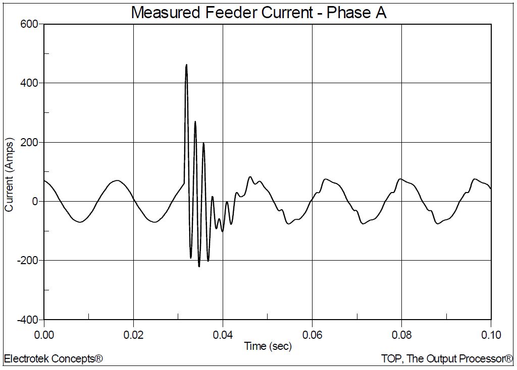
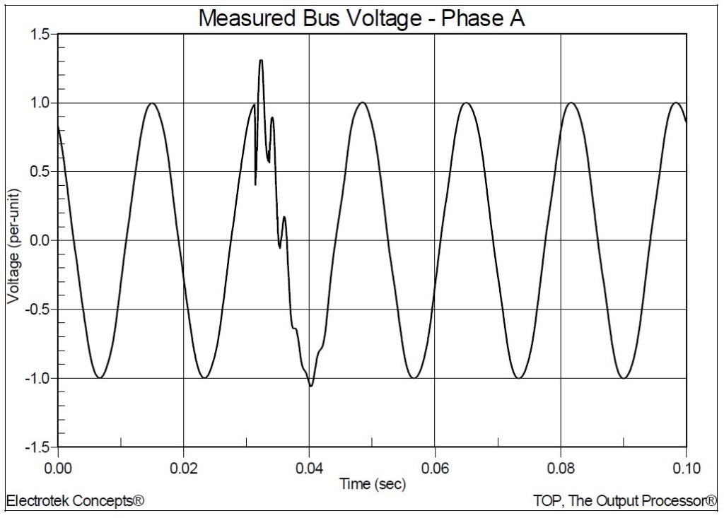
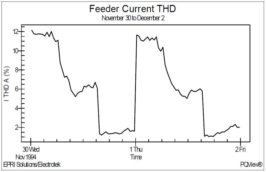
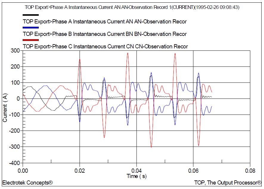
A power quality monitoring example specific to a distribution capacitor bank application is shown in the following four figures. Figure 1 shows a 13.8kV distribution feeder current and Figure 2 shows the bus voltage before and after energization of a pole-mounted 900 kVAr capacitor bank. The resulting transient overvoltage is approximately 1.3 per-unit (130%) and the steady-state voltage rise is approximately 1.2%.
Insertion of the capacitor bank creates a harmonic resonance condition on the feeder, thereby increasing the harmonic current distortion recorded by the power quality monitor. The harmonic current distortion before the capacitor bank is energized is approximately 1.8% and the distortion after energization is approximately 11.8%. A spectral analysis of the harmonic current waveform after energization of the capacitor bank shows that the highest harmonic is the 9th.
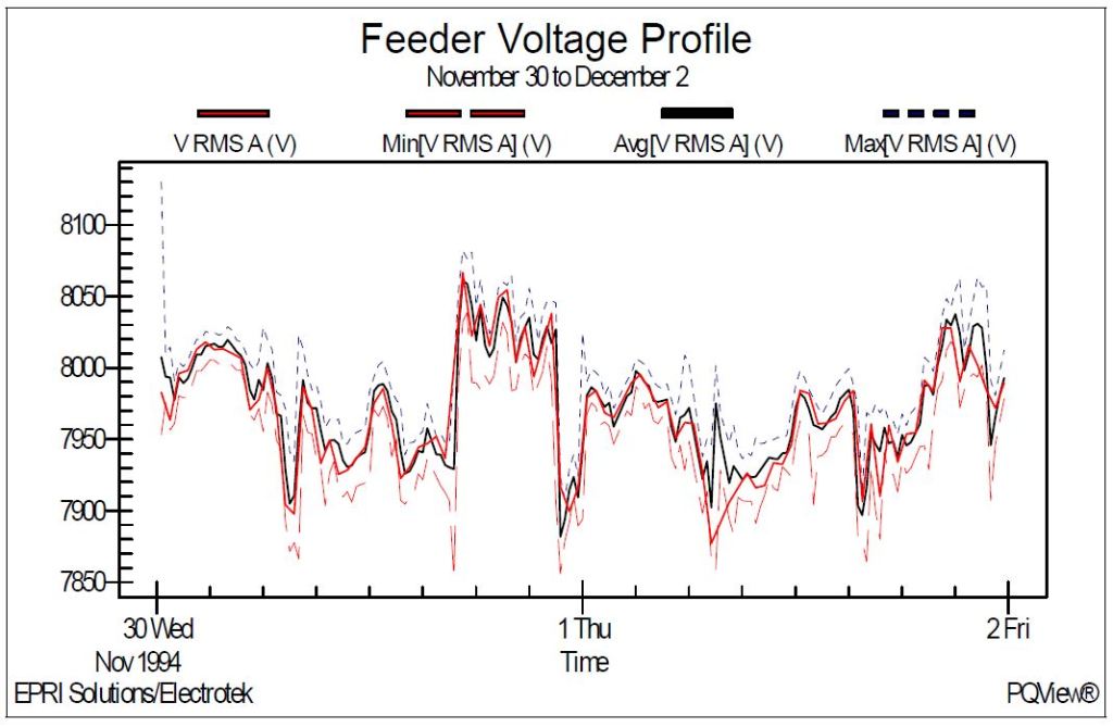
Figure 3 shows the rms voltage trend for the same feeder for a two day period that includes the energization of the feeder capacitor bank. The trend shows the corresponding steady-state voltage rise when the capacitor bank is energized.
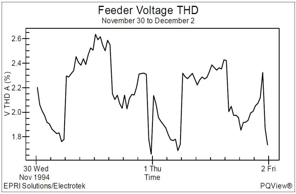
Figure 4 shows the voltage distortion trend and Figure 5 shows the current distortion trend for the same feeder for the same two day period that includes the energization of the feeder capacitor bank. The current distortion before the capacitor bank is energized is approximately 1.8% and the distortion after energization is approximately 11.8%.
Figure 1 – Measured Distribution Feeder Current during Capacitor Bank Energization
Figure 2 – Measured Distribution Feeder Voltage during Capacitor Bank Energization
Figure 3 – Measured Distribution Feeder Voltage Profile
Figure 4 – Measured Distribution Feeder Voltage Distortion Trend
Figure 5 – Measured Distribution Feeder Current Distortion Trend
SUMMARY
Power quality problems encompass a wide range of disturbances and conditions on utility and customer power systems. They include everything from very fast transient overvoltages (microsecond) to long duration outages (hours or days). Power quality problems also include steady-state phenomena such as harmonic distortion, and intermittent phenomena, such as voltage flicker. This wide variety of conditions that make up power quality makes the development of standard measurement procedures and equipment very difficult. This case study introduces the subject of monitoring objectives and screening procedures and provided a distribution feeder capacitor bank application monitoring example.
REFERENCES
IEEE Standard 1159. IEEE Recommended Practice on Monitoring Electric Power Quality. Measuring Voltage and Current Harmonics in Distribution Systems, M. F. McGranaghan, J. H. Shaw, R. E. Owen, IEEE Paper 81WM126-2, November 1981. A Guide to Monitoring Power Quality, EPRI TR-103208, Project 3098-01, Electric Power Research Institute, April 1994.
RELATED STANDARDS IEEE Standard 1159 IEEE Standard 1346 IEEE Standard 1250 IEEE Standard 519
GLOSSARY AND ACRONYMS DFT: Digital Fault Recorders IEEE: Institute of Electrical and Electronics Engineers PQDA: Power Quality Data Analyzer PQDM: Power Quality Data Manager TDD: Total Demand Distortion UPS: Uninterruptible Power Supply
Published by Electrotek Concepts, Inc., PQSoft Case Study: Transformer Energizing and Dynamic Overvoltages, Document ID: PQS0709, Date: October 15, 2007.
Abstract: Energizing power transformers results in inrush currents that are rich in harmonic components. The inrush current interacts with the system impedance vs. frequency characteristics to create a voltage waveform that can have significant harmonic components for the duration that the inrush current is present.
Dynamic overvoltages are long-term resonant overvoltages lasting many cycles that can cause damage to capacitor units and other adjacent equipment, such as transformers and surge arresters.
This case study presents a transformer energizing and dynamic overvoltage evaluation for a 34.5kV distribution system.
INTRODUCTION
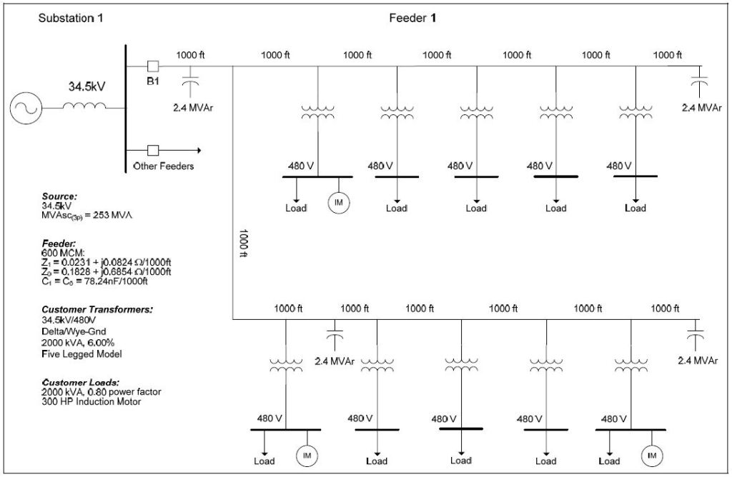
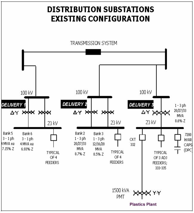
A transformer energizing and dynamic overvoltage evaluation was completed for the system shown in Figure 1.
Figure 1 – Oneline Diagram for Transformer Energizing and Dynamic Overvoltage
BACKGROUND
Energizing saturable devices (devices with magnetic cores), such as power transformers, results in inrush currents that are rich in harmonic components. The inrush current interacts with the system impedance vs. frequency characteristics to create a voltage waveform that can have significant harmonic components for the duration that the inrush current is present. Transformer inrush current typically decays over a period on the order of one second.
This phenomenon combines concerns for harmonic current distortion and transient voltages. The harmonics of concern are low order (dominated by the 2nd through the 5th harmonics). If the circuit has a high impedance resonance near one of these frequencies, a dynamic overvoltage condition results that can cause failure of arresters and problems with sensitive equipment.
This problem is typically limited to cases of energizing large transformers with large power factor correction capacitor banks (e.g., arc furnace installations or other large industrial facilities). The solution to problems with dynamic overvoltages is to assure that the conditions causing the system resonance are not present when the transformer is energized. This could mean making sure a capacitor bank is out of service whenever a large transformer is energized.
Figure 2 shows an example measured current waveform on a 12.5kV feeder during a transformer energizing operation.
Figure 2 – Example Transformer Inrush Current during Circuit Restoration
SIMULATION RESULTS
The accuracy of the system model was verified using three-phase and single-line-to-ground fault currents and other steady-state quantities, such as transformer, load, and capacitor bank rated currents and voltage rise.
The initial case (Case 1a) involved energizing the 18 MVA transformer using the high-side circuit breaker T1 with no secondary load or the 3.6 MVAr capacitor bank in-service on the 34.5kV bus. Figure 3 shows the worst-case simulated primary transformer current (Phase A) during energization of the unloaded transformer. The peak inrush current is nearly 175 amps. For reference, the full-load current for the transformer is approximately 45 amps. Figure 4 shows the corresponding secondary 34.5kV bus voltage waveform, which contains virtually no distortion.
Figure 3 – Transformer Energizing Primary Inrush Current
Figure 4 – Transformer Secondary Voltage during Transformer Energizing
Transformer inrush current is rich in 2nd, 3rd, 4th, and 5th harmonics. The exact characteristics of the inrush current are dependent on transformer parameters (e.g., saturation curve) and the initial condition of the residual transformer flux.
The second case (Case 1b) involved energizing the 18 MVA transformer using the high-side circuit breaker T1 with no secondary load and with the 3.6 MVAr capacitor bank in-service on the 34.5kV bus.
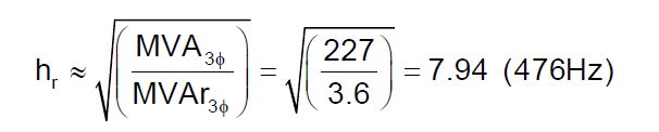
The resonant frequency for the 18 MVA transformer and the 3.6 MVAr capacitor bank may be approximated using the following expression:
where: hr = parallel resonant frequency (x fundamental) MVA3φ = three-phase short circuit capacity (MVA = √3 * 34.5 kV * 3.8 kA ≈ 227 MVA) MVAr3φ = three-phase capacitor bank rating (MVAr)
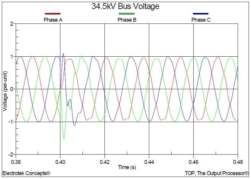
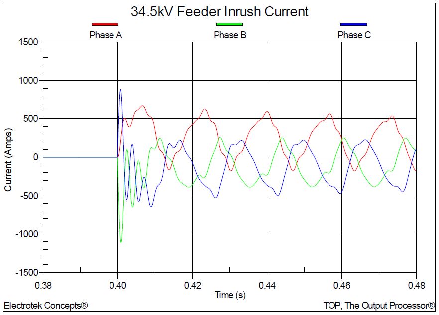
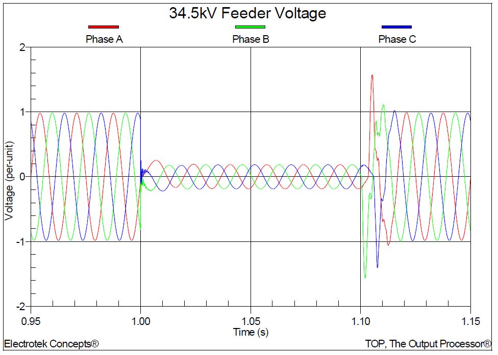
Figure 5 shows the worst-case simulated primary transformer current (Phase A) during energization of the unloaded transformer with the 3.6 MVAr capacitor bank in-service on the 34.5kV bus. Figure 6 shows the corresponding worst-case secondary 34.5kV bus voltage (Phase C).
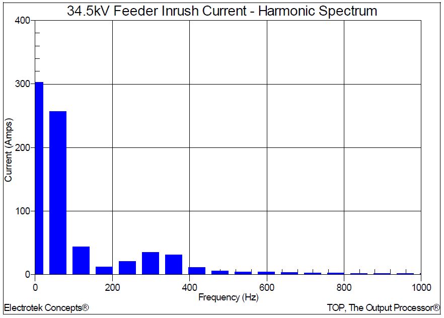
As can be observed from the simulation results, the current waveform is much more distorted than the initial case that did not have the 3.6 MVAr capacitor bank in-service. In addition, the voltage waveform shows a resonance condition and the resulting dynamic overvoltage. Dynamic overvoltages are defined as long-term resonant overvoltages lasting many cycles that can cause damage to capacitor units and other adjacent equipment, such as transformers and surge arresters. Figure 7 shows the results of a Fourier analysis of the voltage waveform. The highest harmonic voltage component is at 480 Hz, which corresponds to the previous resonance calculation.
Figure 5 – Transformer Inrush Current with Secondary Capacitor Bank In-Service
Figure 6 – Transformer Secondary Voltage with Capacitor Bank In-Service
Figure 7 – Transformer Secondary Voltage Harmonic Spectrum
The final case (Case 1c) shows the effect of adding a secondary load on the 34.5kV bus, while still energizing the 18 MVA transformer using the high-side circuit breaker T1 with the 3.6 MVAr capacitor bank in-service. Figure 8 shows the worst-case simulated primary transformer current (Phase A) during energization of the loaded transformer with the 3.6 MVAr capacitor bank in-service on the 34.5kV bus. Figure 9 shows the corresponding worst-case secondary 34.5kV bus voltage (Phase C). As can be observed from the simulation results, the current and voltage waveforms are much less distorted with 5,000 kVA of resistive load included on the 34.5kV bus.
Figure 8 – Transformer Inrush Current with Secondary Load In-Service
Figure 9 – Transformer Secondary Voltage with Secondary Load In-Service
CONCLUSIONS
Observations and conclusions for this case study include:
− Transformer inrush currents contain harmonic currents that may produce dynamic overvoltages if the transformer is energized with a capacitor bank on the secondary bus.
− Solutions to this problem include energizing the capacitor bank separately from the transformer (this prevents the inrush current from exciting the resonant circuit) and energizing the transformer/capacitor combination with enough secondary load to sufficiently damp the transient overvoltage. The combination of switching an unloaded transformer and capacitor bank is the most susceptible to dynamic overvoltages.
RELATED STANDARDS IEEE Std. 1036
GLOSSARY AND ACRONYMS MOV: Metal Oxide Varistor Arrester MSSPL: Maximum Switching Surge Protective Level SiC: Silicon Carbide Arrester
Published by Electrotek Concepts, Inc., PQSoft Case Study: ModelingFerroresonance in an Underground Distribution System, Document ID: PQS0610, Date: July 1, 2006.
Abstract: The objective of this case study is to provide an overview of ferroresonance phenomena, its modeling aspects, and practical experience in recognizing, avoiding, and solving the problem. In particular, it will present symptoms of ferroresonance. An actual example simulation analysis involving an underground cable circuit with blown fuses is presented along with solutions to avoid ferroresonance.
INTRODUCTION
Ferroresonance is a general term applied to a wide variety of resonance interactions involving capacitors and saturable iron-core inductor. During the resonance the capacitive and inductive reactances are equal with opposite values, thus the current is only limited by the system resistance resulting in unusually high voltages and/or currents. Ferroresonance in transformers are more common than any other power equipment since their cores are made of saturable ferrous materials.
Ferroresonant overvoltages on distribution systems were observed early in the history of power systems (i.e., early 1900s). In this case study, the theory of ferroresonance is briefly presented. More theoretical description can be found in documents listed in the reference section. Symptoms of ferroresonance and personal accounts of engineers who witnessed the phenomena are provided. Ferroresonant modeling and a case study of an actual ferroresonance problem with its corresponding solutions is also included in the case.
PRINCIPLES OF FERRORESONANCE
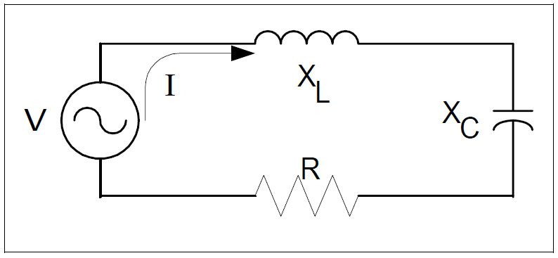
There are various ways to understand ferroresonance. One method is to begin with a review of a simple RLC circuit. Figure 1 shows a voltage source with an arbitrary frequency, such as 50 Hz or 60 Hz.
Figure 1 – Simple RLC Circuit for Explaining Ferroresonance
The inductive (XL) and capacitive (XC) reactances are assumed to be constant or linear. Furthermore, it is assumed that the resistance (R) is much smaller than |XL| and |XC|. The magnitude of current flowing in the circuit is approximately:
I = V / R + XL – XC ≅ V / XL – XC
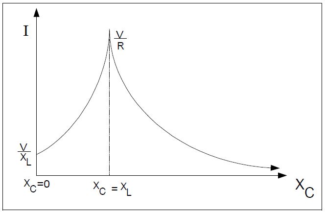
Let us vary XC and hold R and XL at a constant value. When XC = 0, the current flowing in the circuit is I=V/ XL, and when XC is very large, the current becomes negligible. In between these two extremes, |XC|=|XL|. The current becomes very large limited only by R, i.e., I=V/ R. The large current can produce considerable overvoltage. Figure 2 illustrates the magnitude of current under various XC values. The possibility of XC exactly matching XL is remote since both values are linear or constant. However, if the value of XL varies, such as in an iron core transformer, the possibility of XC equaling XL increases considerably.
Figure 2 – Current in the Simple Series RLC Circuit with Various XC Values
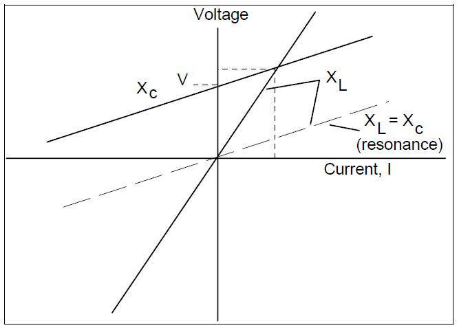
Alternatively, the solution to the above circuit can be written as follows:
VL = jXLI = V – (-jXC)I or, v = XLI, and v = V – XCI
where V is an arbitrary voltage.
Figure 3 – Graphical Solution of Linear LC Circuit
The intersection between the inductive reactance XL line and the capacitive reactance XC line yields the current in the circuit and the voltage across the inductor, VL. The above solution is depicted in Figure 3. At resonance, these two lines become parallel, yielding solutions of infinite voltage and current (assuming lossless element).
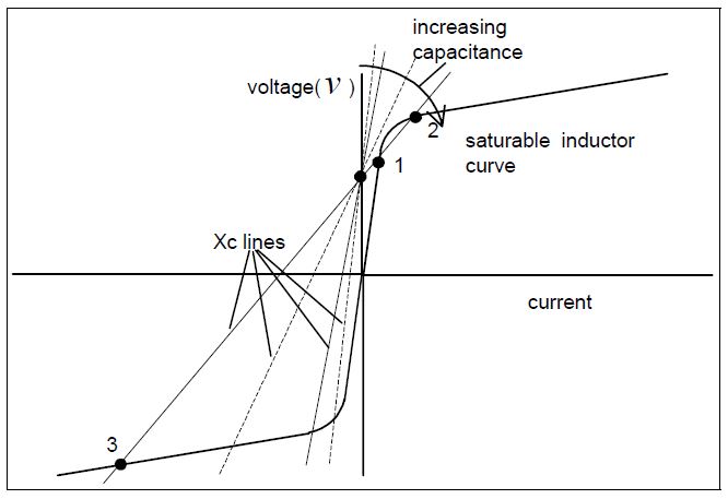
When XL is no longer linear, such as a saturable inductor, the XL reactance can no longer be represented with a straight line. The graphical solution is now as shown in Figure 4.
Figure 4 – Graphical Solution of a Nonlinear LC Circuit
It is obvious that there may be as many as three intersections of the capacitive reactance line with the inductive reactance curve. Intersection 2 is an unstable operating point and the solution will not remain there in steady-state. However, it may pass through this point during a transient. Intersections 1 and 3 are stable and will exist in steady-state. Obviously, if the values become an intersection 3 solution, there will be both high voltages and high currents. For small capacitances, the XC line is very steep, usually resulting in only one intersection in the third quadrant. The capacitive reactance is larger than the inductive reactance, resulting in a leading current and higher than normal voltages across the capacitor. The voltage across the capacitor is the length of the line from the system voltage intersection to the intersection with the inductor curve. As the capacitance increases, there can be multiple intersections as shown. The natural tendency then is to achieve a solution at intersection 1, which is an inductive solution with lagging current and little voltage across the capacitor. Note that the voltage across the capacitor will be the line-to-ground voltage on the cable in a typical power system ferroresonance case.
If there is a slight increase in the voltage, the capacitor line would shift upward, eliminating the solution at intersection 1. The solution would then try to jump to the third quadrant. Of course, the resulting current might be so large that the voltage drops again and the solution point jumps between 1 and 3. Indeed, phenomena like this are observed during instances of ferroresonance. The voltage and current appear to vary randomly and unpredictably.
In the usual power system case, ferroresonance occurs when a transformer becomes isolated on a cable section in such a manner that the cable capacitance appears to be in series with the magnetizing characteristic of the transformer. For short lengths of cable, the capacitance is very small and there is one solution in the third quadrant at relatively low voltage levels. As the capacitance increases the solution point creeps up the saturation curve in the third quadrant until the voltage across the capacitor is well above normal. These operating points may be relatively stable, depending on the nature of the transient events that precipitated the ferroresonance.
SYMPTOMS OF FERRORESONANCE
There are several modes of ferroresonance with varying physical and electrical characteristics. Some have very high voltages and currents while others have voltages close to normal. In this section symptoms of ferroresonance are presented.
Audible Noise
One thing common to all types of ferroresonance is that the steel core is driven into saturation, often deeply and randomly (otherwise, it is conventional resonance and not considered ferroresonance). As the core goes into a high flux density, it will make an audible noise due to the magnetostriction of the steel and to the actual movement of the core laminations. In ferroresonance, this noise is often likened to shaking a bucket of bolts, whining, or to a chorus of a thousand hammers pounding on the transformer from within. In any case, the sound is distinctively different and louder than the normal hum of a transformer.
Overheating
Another reported symptom of the high magnetic field is due to stray flux heating in parts of the transformer where magnetic flux is not expected. Since the core is saturated repeatedly, the magnetic flux will find its way into the tank wall and other metallic parts. One possible side effect is the charring or bubbling of paint on the top of the tank. This is not necessarily an indication that the unit is damaged, but damage can occur in this situation if the ferroresonance has persisted sufficiently long to cause overheating of some of the larger internal connections. This may in turn damage insulation structures beyond repair.
Arrester and Surge Protector Failure
The arrester failures are related to heating of the arrester block. One common failure scenario is for line personnel to discover an open fused cutout and to simply replace the fuse. Meanwhile, the arrester on that phase has become very hot and goes into thermal runaway upon restoration of full power to that phase. Failures are often catastrophic with parts being expelled from the arrester housing. Under-oil arresters are less susceptible to this problem because they are able to dissipate the heat due to the ferroresonance current more rapidly.
Flicker
Customers are frequently subjected to a wavering voltage magnitude. Light bulbs will flicker between very bright and dim. Some electronic appliances are reportedly very susceptible to the voltages that result from some types of ferroresonance, but we have no knowledge of the alleged failure mode. Perhaps, it is simply MOV failure in the power front end. These frequently fail catastrophically, going into thermal runaway and then burning open with considerable arcing display. This may do nothing more than pop a breaker, but surge protection is lost for any subsequent surge that might damage the appliance.
Cable Switching
The transformers themselves can usually withstand the overvoltages without failing. Of course, they would not be expected to endure this stress repeatedly because the forces often shake things loose inside and abrade insulation structures. The cable is also in little danger unless its insulation stress had been reduced by aging or physical damage. Of course, operating a solid dielectric system above its normal stress level for an extended period can be expected to create some shortage of life.
It may be difficult to clear arcs when pulling cable elbows if ferroresonance is in progress. The currents may be much higher than expected and the peak voltages may be high enough to cause reignition of the arc.
Some utilities will not perform cable switching involving three-phase padmount transformers without first verifying that there is substantial load on the transformers. One of the common solutions to ferroresonance during cable switching is to always pull the elbows and energize the unit at the primary terminals. This will normally work because there is no external cable capacitance to cause ferroresonance. There is little internal capacitance, and the losses of the transformers are usually sufficient to prevent resonance with this small capacitance. Unfortunately, modern transformers are changing the old rules of thumb. The newer low-loss transformers, particularly, those with amorphous metal core, are prone to ferroresonance.
TRANSFORMER MODELING
Ferroresonance can be mysterious subject. Probably the main reason is that the analysis requires sophisticated nonlinear circuit analysis techniques. The results are sometimes unpredictable and certainly difficult to visualize (unlike linear circuit phenomena). Another issue that complicates the analysis of ferroresonance is that there are several different types of three-phase transformers such as three single-phase transformers connected as a three-phase transformer, three-legged core transformers, three-phase shell-type transformers, four-legged core, and five-legged cores. The conventional T model of a two-winding transformer, and the five-legged core transformer model will be summarized in this section.
For single-phase transformers, three-phase shell form transformers, and three-phase triplexed transformers (three single-phase units stacked in one can), the conventional T model will suffice because there is no coupling between the magnetic circuits. Figure 5 shows the T model for a two winding transformer, which will suffice for standard switching surge and ferroresonance studies. For higher frequencies, it would be necessary to model the capacitances and inner winding construction.
Figure 5 – Standard T Model of a Two-Winding Transformer
The terminals of this model can be connected to represent any two-winding transformer with magnetically independent phases. The saturable inductance data are readily available from the manufacturer’s test data. Note that manufacturers supply the rms v-i curve. This must be converted to a peak flux-current curve before it can be used in EMTP or other transients programs. This conversion is a bit tricky because the current waveforms are not sinusoidal. Therefore, one cannot simply multiply the current values on the rms curve by 1.414 to determine the correct peak value. The usual procedure is to use a computer program that reconstructs the peak saturation curve by iterative solution. The first point can be established by multiplying by 1.414. Then a guess is made at the next point and the waveform is reconstructed. The guess is adjusted until the rms of the reconstructed waveform matches that supplied by the manufacturer.
The five-legged core transformer design [3] is illustrated in Figure 6. The design typically consists of four individual cores tied together to create the five-legged core transformer. The inner three legs carry the phase windings with flux paths as indicated. The equivalent circuit can be derived from the flux path direction and is shown in Figure 7.
Figure 6 – Five-Legged Transformer Design and its Flux Paths
Figure 7 – Equivalent Circuit for a Five-Legged Transformer
CASE STUDY
In this section, an actual case study is presented. A ferroresonance condition developed on an approximately 5,000-foot underground cable feed to a medical facility. When one of the riser pole fuses blew, severe voltage fluctuations occurred at the load. As a temporary solution the utility replaced the fuses with a three-phase recloser and wanted to see under what conditions the three-phase recloser might be removed and the fuses reinstalled. Therefore, the purpose of this case study was to determine under what conditions the ferroresonance at the underground distribution network could be avoided (and whether fuses might be reinstalled instead of keeping the three-phase recloser).
The ferroresonance condition apparently did not cause damages to the two 500 kVA transformers nor the customer loads at the medical facility. However, it was reported that a sudden overvoltage did occur and lights flickered between bright and dim.
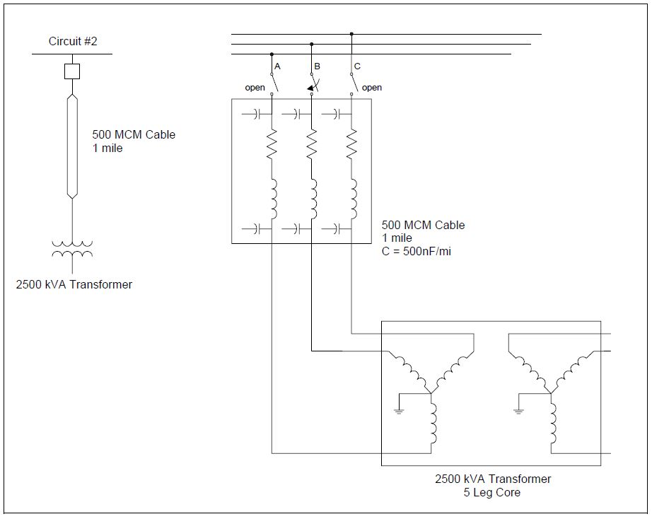
A simplified one-line diagram to study the ferroresonance problem is shown in Figure 8. The simulation model was developed using the EMTP program.
Figure 8 – Oneline Diagram fro the Underground Cable-Fed Run
The lengths of the cable from the first pole to the first switch (S1), and from the first switch (S1) to the second switch (S2) were approximately 1,900 feet and 2,150 feet long. The cable size was 600 MCM with the following characteristics:
Insulation: 0.1406 outside diameter in feet Jacket: 0.1412 outside diameter in feet Neutral: 0.1409 outside diameter in feet
A line constant program was used to compute the positive and zero-sequence impedances of the cable, yielding the following results:
The lengths of the underground cable from the second switch (S2) to the first transformer (JL61), and from the first transformer (JL61) to the second transformer (KL30) were 420 and 450 feet long, respectively. The type of the cable was 1/0 with the following characteristics:
Insulation: 0.0629 outside diameter in feet Jacket: 0.0688 outside diameter in feet Neutral: 0.0794 outside diameter in feet
The computed positive and zero-sequence impedances were:
The two 500 kVA transformers were modeled according to the five-legged core transformer design. In order to investigate overvoltage due to ferroresonance, one phase of the cable was intentionally opened to simulate circumstances leading to ferroresonance (e.g., fuse blows, cable connector or splice opening, etc.). In the simulation, phase B at the first pole was open-circuited, while switches S1 and S2 shown in Figure 8 were closed at all times. Resistive loads at the secondary winding of transformers JL61 and KL30 were increased from zero to 30% of the transformer capacities, i.e., from 0 to 150 kW.
Figure 9 shows voltage waveforms at the secondary winding of transformer JL61 when both JL61 and KL30 transformers are unloaded. Since the voltage at the secondary of transformer KL30 is nearly identical to that of JL61, the voltage waveforms are not shown. Industry analysts have historically assumed that when the voltage exceeds 1.25 per-unit, the system is said to be “in ferroresonance”. Figure 9 clearly illustrates that the system is in ferroresonance condition since phase B exhibits sustained overvoltage approaches 3.0 per-unit.
Figure 9 – Voltage Waveforms at Secondary Winding of Transformer JL61
Figure 10 (top left) shows the voltage waveforms at the secondary winding of JL61 transformer when both JL61 and KL30 transformers are loaded with resistive load equivalent to 5% of transformer capacities. In other words, JL61 and KL30 transformers are loaded with 25 kW loads. The overvoltage at phase B is now approximately 2 per-unit, much less compare to when both transformers are unloaded.
In the similar fashion, loads at both transformers are added successively, i.e., 10, 15, 20, 25, and 30% of the transformer capacities. As loads increase the overvoltage drops quickly. Figure 10 shows the voltage waveforms at the secondary winding of transformer JL61 when both transformers are loaded with 5% (top left), 15% (top right), 20% (bottom left), and 30% (bottom right) of their respective capacities.
With 15% of load, the system remains in ferroresonance condition since it exhibits sustained overvoltage of 1.5 per-unit. The ferroresonance condition is practically eliminated when both transformers are loaded with 20% of resistive load. The overvoltage magnitude is about 1.4 per-unit at when phase B is open, however this overvoltage is not sustained and quickly decays to a low voltage. With 30% of load, the system is not in ferroresonance either. Twenty percent of resistive load is sufficient to avoid the ferroresonance condition.
Figure 10 – Voltage Waveforms at the Secondary Winding of Transformer JL61 (with (a) 5%, (b) 15%, (c) 20%, and (d) 30% of their Respective Capacities)
Figure 11 shows the summary of peak overvoltages when both transformers are loaded from 0% to 30% of their capacities. The overvoltage on phase B drops quickly as both transformers become more loaded. From the analysis presented in this section, it can be concluded that both transformers should be loaded with a minimum of 100 kW resistive load or loads equivalent to 20% of transformer capacity to avoid the ferroresonance condition. The rapid drop in ferroresonant voltage magnitude is due in large part to the introduction of the resistive load.
Based on the study, the ferroresonance condition can be avoided by having both transformers loaded with at least 20 percent of their respective capacities. In other words, each transformer must have 100 kW (resistive) at its secondary winding. When one phase is open-circuit, there will be a momentary overvoltage as high as 1.4 per-unit, however it quickly decays to a low voltage. There will be no sustained ferroresonance overvoltage. If this minimum loading can be guaranteed, it is safe to replace a three-phase recloser with three fuses.
In the event that the loading cannot be achieved, it is advised to use the three-phase switchgear to avoid the ferroresonance condition. The minimum load of 20% to avoid ferroresonance is much higher than the usual minimum load of 5%. The higher minimum is primarily due to the length of the cable involved, which is approximately 1 mile long.
Figure 11 – Change in Peak Transient Overvoltage vs. % Resistive Load on a 500kVA Transformer
SUMMARY
A fundamental description of ferroresonance has been presented in this case study. In particular, analysis of the ferroresonance condition based on a simple graphical approach is presented. Several transformer models are also included for reference. Finally, a representative case study showing ferroresonance in an underground cable circuit is included. Minimum load levels for mitigating ferroresonance are evaluated.
REFERENCES
[1] R. Rudenberg, Transient Performance of Electric Power Systems, New York, NY, McGraw-Hill Company, 1950. [2] C. Hayashi, Nonlinear Oscillations in Physical Systems, New York, NY, McGraw-Hill Company, 1964. [3] D. L. Stuehm, B. A. Mork, D. D. Mairs, “Five-legged core transformer equivalent circuit”, IEEE Transactions on Power Delivery, Vol 4, No. 3, July 1989, pp. 1786. [4] Slow Transient Task Force of the IEEE Working Group on Modeling and Analysis of System Transients Using Digital Programs, “Modeling and analysis guidlines for slow transients – Part III: The study of ferroresonance,” IEEE Trans. on Power Delivery, vol. 15, No. 1., Jan. 2000, pp. 255 – 265.
RELATED STANDARDS IEEE Std. C57.105-1978
GLOSSARY AND ACRONYMS MOV: Metal Oxide Varistor Arrester MSSPL: Maximum Switching Surge Protective Level SiC: Silicon Carbide Arrester
Published by Electrotek Concepts, Inc., PQSoft Case Study: General Reference – Ferroresonance, Document ID: PQS0607, Date: July 1, 2006.
Abstract: The term ferroresonance refers to a special kind of resonance that involves capacitor and iron-core inductance. The most common condition in which it causes disturbances is when the magnetizing impedance of a transformer is placed in series with a system capacitor. There are several modes of ferroresonance with varying physical and electrical characteristics. Some have very high voltages and currents, while others have voltages close to normal. There may or may not be equipment failures or other evidence of ferroresonance in the electrical equipment. In many cases it may be may be difficult to tell if ferroresonance has occurred, unless there are witnesses or power quality monitoring instruments installed.
This case presents an overview of ferroresonance and a number of example measured and simulated waveforms.
OVERVIEW OF FERRORESONANCE
Ferroresonance is a term generally applied to a wide variety of interactions between capacitors and iron-core inductors that result in unusual voltage and/or currents. In linear circuits, resonance occurs when the capacitive reactance equals the inductive reactance at the frequency at which the circuit is excited. Iron-core inductors have a nonlinear characteristic and therefore a range of inductance values. This relationship may lead to a number of operating conditions where the inductive reactance does not equal the capacitive reactance, but very high and damaging overvoltages occur.
In a typical power system, ferroresonance occurs when a transformer becomes isolated on a cable section in such a manner that the cable capacitance appears to be in series with the magnetizing characteristic of the transformer. An unbalanced switching operation is required to initiate the condition.
Several of the more common causes include:
single-phase cutouts
fuse blowing or opening (transformer or line fuse) (or a lineman pulls an elbow connector)
single-phase reclosers
cable connector of splice opening
manual cable switching to reconfigure a cable circuit during an emergency condition
open conductor fault in overhead line feeding cable
three-phase switch with large pole closing span
Two additional conditions must be satisfied for ferroresonance to occur:
The length of cable between the transformer and open conductor location must have sufficient capacitance to produce excessive ferroresonant voltages
The losses in the circuit and the resistive load on the transformer must be low.
These conditions may be met at a variety of times. The low resistive load requirement is often satisfied on new construction projects, when there may be no load on the transformer for a period of time. As the load increases, ferroresonance becomes much less likely (unless the customer separates from the utility during emergency conditions). Figure 1 illustrates one possible switching condition that can lead to ferroresonance. The case, which was investigated using computer simulations, involves a stuck-pole in the feeder switch. A number of different scenarios may lead to this condition, however, for the purposes of simulation, it is simply modeled as two phases open and one closed.
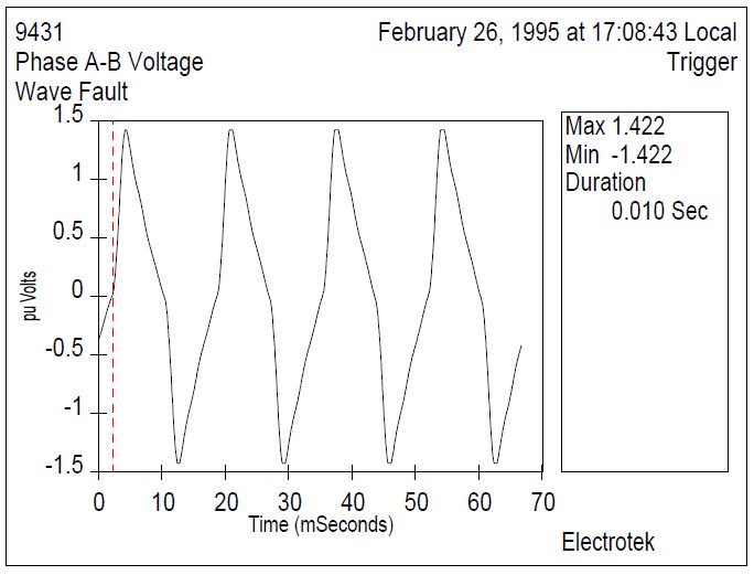
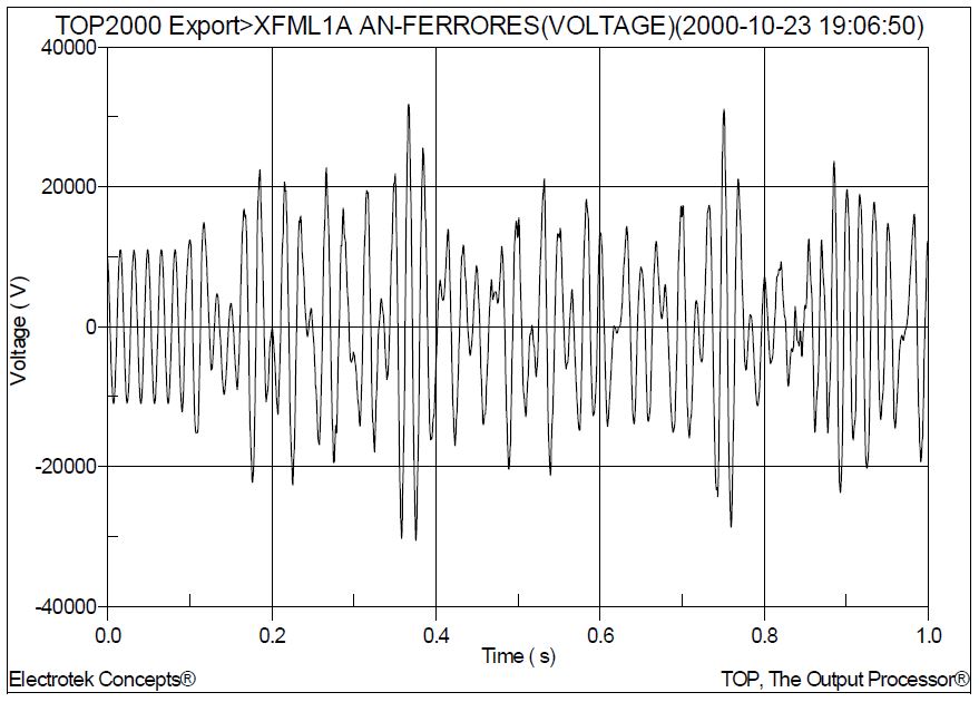
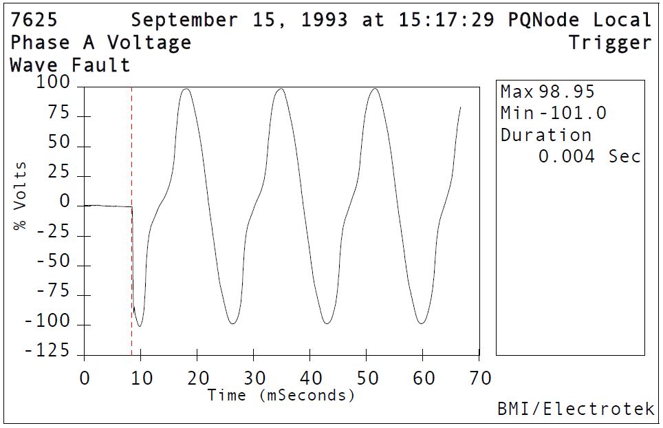
There are several modes of ferroresonance with varying physical and electrical characteristics. Some have very high voltages and currents, while others have voltages close to normal, as illustrated in Figure 2. There may or may not be equipment failures of other evidence of ferroresonance in the electrical equipment. In many cases it may be may be difficult to tell if ferroresonance has occurred, unless there are witnesses or power quality monitoring instruments installed.
Figure 2 – Example Measured Distribution Feeder Voltage during Ferroresonance
One thing common to all types of ferroresonance is that the steel core is driven into saturation, often deeply and randomly (otherwise, it is conventional resonance). As the core goes into a high flux density, it will make an audible noise due to the magnetostriction of the steel and movement of the core laminations. The sound produced is distinctly different and louder than the normal hum of a transformer. Another reported symptom of the high magnetic field is charring or bubbling of the paint on the top of the transformer tank. This is due to stray flux heating in parts of the transformer where magnetic flux is not expected. Since the core is saturated repeatedly, the magnetic flux will find its way into the tank wall and other metallic parts.
If high voltages accompany the ferroresonance, there could be electrical damage to both the primary and secondary circuits. Surge arresters commonly fail during this condition. Arrester failures are related to the heating of the arrester block, and at times, the failures can be catastrophic, with parts being expelled from the arrester housing.
Ferroresonance cannot always be entirely avoided; however, steps can be taken to reduce the probability of occurrence. These include locating fuses or disconnects near the transformer (to minimize capacitance), and using three-phase switches. However, neither of these remedies will provide protection for the broken conductor case. Another common solution involves using grounded-wye / grounded-wye transformers. When each phase is magnetically independent, this connection prevents ferroresonance. However, the common five-legged core design of three-phase padmount transformers is still susceptible to ferroresonance because the phases are magnetically coupled.
FERRORESONANCE WAVEFORM EXAMPLES
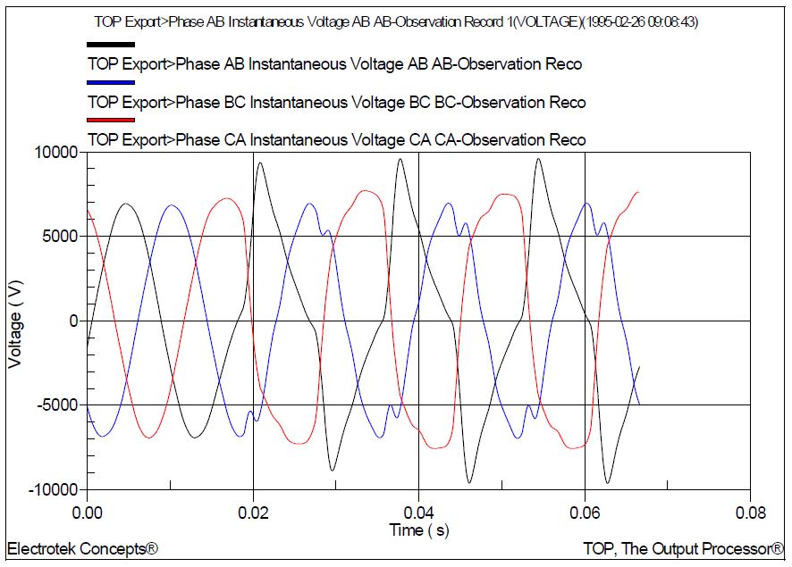
Figure 3 illustrates an example distribution voltage during a ferroresonance event. Phases A-B and C-A are shown. These waveforms were recorded with a Dranetz-BMI 8010 PQNode.
Figure 3 – Example Measured Ferroresonance Voltage Waveform
Figure 4 shows an example simulated distribution system ferroresonance event. This voltage waveform was produced using the Electromagnetic Transients Program (EMTP).
Figure 4 – Example Simulated Ferroresonance Voltage Waveform
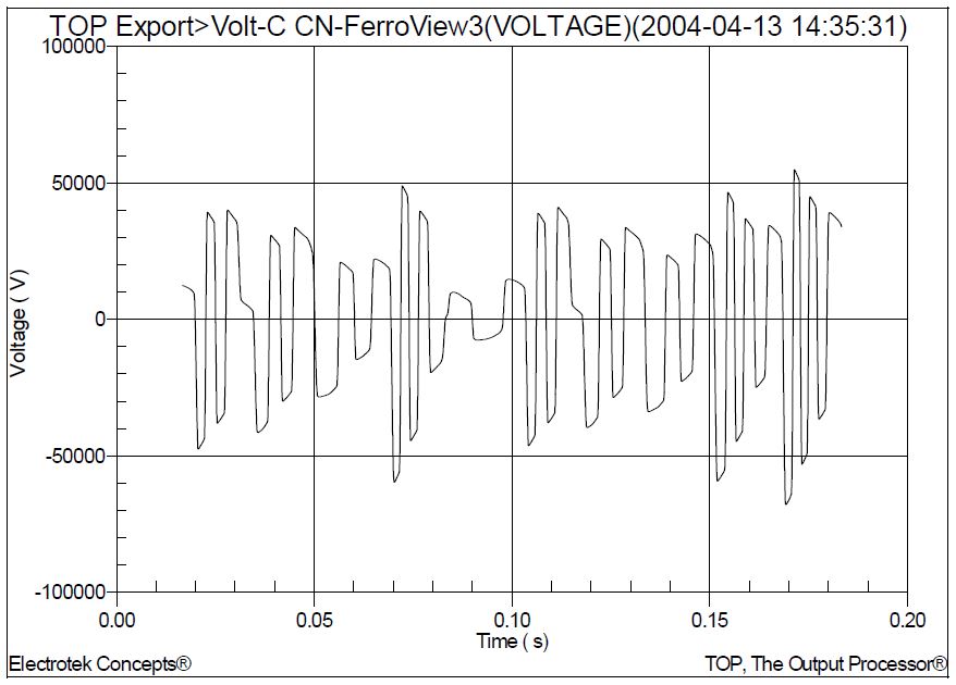
Figure 5 shows an example simulated distribution system ferroresonance event. This voltage waveform was produced using the FerroView program.
Figure 5 – Example Simulated Ferroresonance Voltage Waveform
Figure 6 shows an example simulated distribution system ferroresonance event. This voltage waveform was produced using the PSCAD program.
Figure 6 – Example Simulated Ferroresonance Voltage Waveform
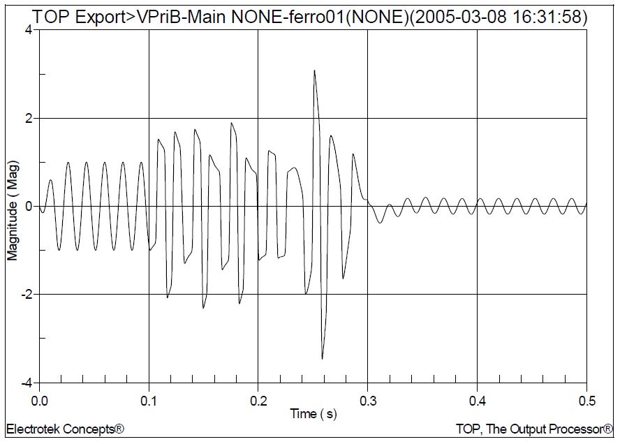
Figure 7 shows an example simulated distribution system ferroresonance event. A resistive load is added to the circuit at 0.3 seconds. This voltage waveform was produced using the PSCAD program
Figure 7 – Example Simulated Ferroresonance Voltage Waveform
Figure 8 shows an example distribution system voltage during a ferroresonance event. These voltage waveforms were recorded with a Dranetz-BMI 8010 PQNode.
Figure 8 – Example Measured Ferroresonance Voltage Waveform
Figure 9 shows an example distribution system feeder current during a ferroresonance event. These current waveforms were recorded with a Dranetz-BMI 8010 PQNode.
Figure 9 – Example Measured Ferroresonance Current Waveform
SUMMARY
Ferroresonance is a term generally applied to a wide variety of interactions between capacitors and iron-core inductors that result in unusual voltage and/or currents. These interactions may lead to a number of operating conditions where high and damaging overvoltages occur. Ferroresonance is different than resonance in linear system elements. In linear systems, resonance results in high sinusoidal voltages and currents of the resonant frequency. Ferroresonance can also result in high voltages and currents, but the resulting waveforms are usually irregular and chaotic in shape, as illustrated with the example waveforms in the case study.
REFERENCES
Tennessee Valley Public Power Association, Inc., Power Quality Manual, Final Report, Project PQ 2, 2002.
RELATED STANDARDS IEEE Std. C57.105-1978
GLOSSARY AND ACRONYMS MOV: Metal Oxide Varistor Arrester MSSPL: Maximum Switching Surge Protective Level SiC: Silicon Carbide Arrester
Published by Siemens Canada, Siemens Limited Power Product Catalogue, Canadian Edition 2019. Section 18 – Technical, Contents: Harmonics / K-factor Ratings (18-16, 18-17)
Non-Linear Loads
When a sinusoidal voltage is applied to a linear load, the resultant current waveform takes on the shape of a sine wave as well. Typical linear loads are resistive heating and induction motors. In contrast, a non-linear load either:
Draws current during only part of the cycle and acts as an open circuit for the balance of the cycle,
or
Changes the impedance during the cycle, hence the resultant waveform is distorted and no longer conforms to a pure sine wave shape
In recent years, the use of electronic equipment has mushroomed in both offices and industrial plants. These electronic devices are powered by switching power supplies or some type of rectifier circuit. Examples of these devices used in offices are: computers, fax machines, copiers, printers, cash registers, UPS systems, and solid-state ballasts. In industrial plants, one will find other electronic devices such as variable speed drives, HID lighting, solid-state starters and solid-state instruments. They all contribute to the distortion of the current waveform and the generation of harmonics. As the use of electronic equipment increases and it makes up a larger portion of the electrical load, many concerns are raised about its impact on the electrical power supply system.
Harmonics
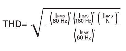
As defined by ANSI / IEEE Std. 519-1992, harmonic components are represented by a periodic wave or quantity having a frequency that is an integral multiple of the fundamental frequency. Harmonics are voltages or currents at frequencies that are integer multiples of the fundamental (60 Hz) frequency: 120 Hz, 180 Hz, 240 Hz, 300 Hz, etc. Harmonics are designated by their harmonic number, or multiple of the fundamental frequency. Thus, a harmonic with a frequency of 180 Hz (three times the 60 Hz fundamental frequency) is called the 3rd harmonic. Harmonics superimpose themselves on the fundamental waveform, distorting it and changing its magnitude. For instance, when a sine wave voltage source is applied to a non-linear load connected from a phase-leg to neutral on a 3-phase, 4-wire branch circuit, the load itself will draw a current wave made up of the 60 Hz fundamental frequency of the voltage source, plus 3rd and higher order odd harmonic (multiples of the 60 Hz fundamental frequency), which are all generated by the non-linear load. Total Harmonic Distortion (THD) is calculated as the square root of the sum of the squares of all harmonics divided by the normal 60 Hz value.
This yields an RMS value of distortion as a percentage of the fundamental 60 Hz waveform.
Therefore, it is the percentage amount of odd harmonics (3rd, 5th, 7th ,…, 25th,…) present in the load which can affect the transformer, and this condition is called a “Non-Linear Load” or “Non-Sinusoidal Load”. To determine what amount of harmonic content is present, a K-Factor calculation is made instead of using the THD formula. The total amount of harmonics will determine the percentage of non-linear load, which can be specified with the appropriate K-Factor rating.
Figure 30 — Effect of Harmonics on Current Waveform
Typical Symptoms of Harmonic Problems
Distribution / lighting transformers overheating even when measured load current is within transformer rating
Neutral cable / bus overheating even with balanced load
Fuses blowing and circuit breakers tripping at currents within rating
Effect Of Harmonics On Transformers
Non-sinusoidal current generates extra losses and heating of transformer coils thus reducing efficiency and shortening the life expectancy of the transformer. Coil losses increase with the higher harmonic frequencies due to higher eddy current loss in the conductors. Furthermore, on a balanced linear power system, the phase currents are 120 degrees out of phase and offset one another in the neutral conductor. But with the “Triplen” harmonics (multiple of 3) the phase currents are in phase and they are additive in this neutral conductor. This may cause installations with non-linear loads to double either the size or number of neutral conductors.
Measurement of Harmonics
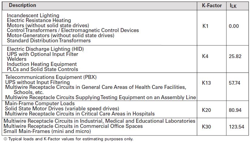
Table A.3 K-Factor Ratings
Sizing Transformers for Non-Linear Loads
ANSI / IEEE C57.110-2008 has a procedure for de-rating standard distribution transformers for non-linear loading. However this is not the only approach. A transformer with the appropriate K-Factor specifically designed for non-linear loads can be specified.
K-Factors
K-Factor is a ratio between the additional losses due to harmonics and the eddy losses at 60 Hz. It is used to specify transformers for non-linear loads. Note that K-Factor transformers do not eliminate harmonic distortion; they withstand the non-linear load condition without overheating.
Calculating K-Factor Loads
List the kVA value for each load category to be supplied. Next, assign a K-factor designation that corresponds to the relative level of harmonics drawn by each type of load. Refer to Table A.4
Multiply the kVA of each load or load category times the Index of Load K-rating (ILK) that corresponds to the assigned K-factor rating. This result is an indexed kVA-ILK value. KVA x ILK = kVA-ILK.
Tabulate the total connected load kVA for all load categories to be supplied.
Next, add-up the kVA-ILK values for all loads or load categories to be supplied by the transformer.
Divide the grand total kVA-ILK value by the total kVA load to be supplied. This will give an average ILK for that combination of loads. Total kVA-ILK/ Total kVA = average ILK.
From Table A.4 find the K-factor rating whose ILK is equal to or greater than the calculated ILK
Measurement of Harmonics Table A.3 K-Factor Ratings
For existing installations, the extent of the harmonics can be measured with appropriate instruments commonly referred to as “Power Harmonic Analyzers”. This service is offered by many consulting service organizations. For new construction, such information may not be obtainable. For such situations, it is best to assume the worse case condition based on experience with the type and mix of loads.
Published by Electrotek Concepts, Inc., PQSoft Case Study: Ferroresonance in an Underground Distribution System, Document ID: PQS0710, Date: October 15, 2007.
Abstract: The term ferroresonance refers to a special kind of resonance that involves capacitor and iron-core inductance. The most common condition in which it causes disturbances is when the magnetizing impedance of a transformer is placed in series with a system capacitor. There are several modes of ferroresonance with varying physical and electrical characteristics. Some have very high voltages and currents, while others have voltages close to normal. There may or may not be equipment failures or other evidence of ferroresonance in the electrical equipment. In many cases it may be may be difficult to tell if ferroresonance has occurred, unless there are witnesses or power quality monitoring instruments installed.
This case study presents a ferroresonance evaluation for a 34.5kV underground distribution system.
INTRODUCTION
An underground distribution system ferroresonance evaluation was completed for the system shown in Figure 1.
Figure 1 – Oneline Diagram for Underground Distribution Ferroresonance
BACKGROUND
Ferroresonance is a term generally applied to a wide variety of interactions between capacitors and iron-core inductors that result in unusual voltages and/or currents. In linear circuits, resonance occurs when the capacitive reactance equals the inductive reactance at the frequency at which the circuit is excited. Iron-core inductors have a nonlinear characteristic and therefore a range of inductance values. This relationship may lead to a number of operating conditions where the inductive reactance does not equal the capacitive reactance, but very high and damaging overvoltages occur.
In a typical power system, ferroresonance occurs when a transformer becomes isolated on a cable section in such a manner that the cable capacitance appears to be in series with the magnetizing characteristic of the transformer. An unbalanced switching operation is required to initiate the condition. Several of the more common causes include:
− Single-phase cutouts − Fuse blowing or opening (transformer/line fuse, or a lineman pulls an elbow connector) − Single-phase reclosers − Cable connector of splice opening − Manual cable switching to reconfigure a cable circuit during an emergency condition − Open conductor fault in overhead line feeding cable − Three-phase switch with large pole closing span
Two additional conditions must be satisfied for ferroresonance to occur:
− The length of cable between the transformer and open conductor location must have sufficient capacitance to produce excessive ferroresonant voltages. − The losses in the circuit and the resistive load on the transformer must be low.
SIMULATION RESULTS
The accuracy of the system model was verified using three-phase and single-line-to-ground fault currents and other steady-state quantities, such as transformer and customer load rated currents.
A ferroresonance condition developed on a roughly 7,000-foot underground cable supplying a medical facility. Severe voltage fluctuations occurred at the customer load when one of the riser pole fuses blew. As a temporary solution, the utility replaced the fuses with a three-phase recloser. A study was completed to determine under what conditions the three-phase recloser might be removed and the fuses reinstalled.
The ferroresonance condition did not damage the two 500 kVA transformers or the customer loads at the medical facility. However, it was reported that a sudden overvoltage did occur and lights flickered between bright and dim.
The lengths of the cable from the first pole to the first switch (S1), and from the first switch (S1) to the second switch (S2) were approximately 2,750 feet and 3,200 feet long. The cable size was 600 MCM with the following characteristics:
Insulation:……………………………….0.1406 outside diameter in feet Jacket:…………………………………….0.1412 outside diameter in feet Neutral:…………………………………..0.1409 outside diameter in feet
A line constant program was used to compute the positive and zero-sequence impedances of the cable, yielding the following results:
Z1 = 0.0231 + j 0.0824 ohms/1000 ft Z0 = 0.1828 + j 0.6854 ohms/1000 ft C1 = C0 = 78.24 ηF/1000 ft
The lengths of the underground cable from the second switch (S2) to the first transformer, and from the first transformer to the second transformer were 420 and 450 feet long, respectively. The type of the cable was 1/0 with the following characteristics:
Insulation:……………………………….0.0629 outside diameter in feet Jacket:…………………………………….0.0688 outside diameter in feet Neutral:…………………………………..0.0794 outside diameter in fee
The computed positive and zero-sequence impedances were:
Z1 = 0.0803 + j 0.0952 ohms/1000 ft Z0 = 0.4061 + j 0.5150 ohms/1000 ft C1 = C0 = 97.34 ηF/1000 ft
The two 500 kVA transformers were modeled using a five-legged core transformer design. In order to investigate overvoltage due to ferroresonance, one phase of the cable was intentionally opened to simulate the circumstances leading to the ferroresonance (e.g., fuse blows, cable connector or splice opening, etc.) event. In the transient simulation, Phase B at the first pole was open-circuited, while the switches S1 and S2 (refer to Figure 1) were closed at all times. Figure 2 shows the three-phase voltage waveform at the secondary winding of one of the 500 kVA transformers with both of the 500 kVA transformers unloaded (Case 2a). Industry analysts have historically assumed that when the voltage exceeds 1.25 per-unit, the system is said to be in ferroresonance. Figure 2 clearly illustrates that the system is in a ferroresonance condition because Phase A exhibits sustained overvoltages greater than 2.0 per-unit.
Figure 2 – Customer Transformer Secondary Voltage with no Secondary Load
A series of cases were completed to determine the relationship between the amount of customer secondary load and the resulting ferroresonant overvoltages. As the load is increased, the transient overvoltage drops very quickly. Figure 3 shows the three-phase voltage waveform at the secondary winding of one of the 500 kVA transformers with both of the 500 kVA transformers having a resistive load equal to 5% (25 kW) of the transformer rating (Case 2b).
Figure 3 – Customer Transformer Secondary Voltage with 5% Secondary Load
The final case investigates the use of a three-phase recloser rather than three single-phase fuses. Figure 4 shows the three-phase voltage waveform at the secondary winding of one of the 500 kVA transformers with both of the 500 kVA transformers unloaded and with a three-phase switch opening on the primary distribution feeder (Case 2c). No ferroresonance occurs during the three-phase switching.
Figure 4 – Customer Transformer Secondary Voltage with a Three-Phase Switch
CONCLUSIONS
Observations and conclusions for this case study include:
− The term ferroresonance refers to a special kind of resonance that involves a capacitance and a variable iron-core inductance. A 34.5kV underground distribution feeder ferroresonance event occurred when a single-phase riser fuse blows.
− Transient computer simulations of the underground distribution feeder circuit indicated that the ferroresonant overvoltages were very dependent on the circuit configuration (e.g., cable length and capacitance, transformer ratings, etc.) and on the rating of the load on the customer secondary circuits.
− Solutions to the ferroresonance problem generally include adding resistive load to the secondary of each customer transformer. For this circuit configuration, a resistive load representing 5% of the transformer rating significantly reduced the secondary transient overvoltages. In addition, the potential for ferroresonance may be eliminated by using three-phase switches in place of single-phase fuses.
RELATED STANDARDS IEEE C57.105-1978, IEEE Std. 1036
GLOSSARY AND ACRONYMS MOV: Metal Oxide Varistor Arrester MSSPL: Maximum Switching Surge Protective Level SiC: Silicon Carbide Arrester
Published by Electrotek Concepts, Inc., PQSoft Case Study: Ferroresonance Analysis – 25kV Single 5-Legged Core Transformer, Document ID: PQS0318, Date: July 18, 2002.
Abstract: Ferroresonance is a concern for medium voltage underground systems. As part of an evaluation of the design of a new 25kV underground system, the potential for ferroresonance was analyzed. Ferroresonance requires a certain length of cable to generate severe overvoltages. With modern transformers, this length is frequently less than 200 ft. Our calculations suggest that the threshold of ferroresonance is about 100 ft for a modern 2500 kVA transformer and 1000 kcmil cable and it is certainly in ferroresonance at 200 ft. These distances are proportionately shorter for smaller transformers. This makes it more difficult to achieve ferroresonance-free installations where single-phase switching or fusing is permitted because the maximum cable length is impractically short. As a general guideline, three-phase switching should be strongly considered for cable length exceeding 100 ft. If the switchgear can be mounted closer to the transformer, fused switching may be used with little fear of serious overvoltages.
PROBLEM STATEMENT
An electric utility was evaluating the proposed design of a new, predominantly underground, 25kV system. One of the concerns of the utility related to the new system was the likelihood of 25kV transformers experiencing ferroresonant conditions. This case study was an effort to characterize the combinations of parameters that would increase the probability of ferroresonance.
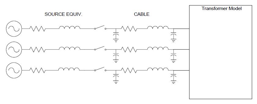
SYSTEM MODEL
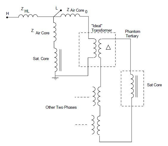
The complete three-phase schematic of the circuit used to evaluate ferroresonance on a single 5-legged core transformer is shown in Figure 1.
Figure 1: Circuit Model used for Ferroresonance Study.
This model was represented in the EMTP program and executed for a number of cases. The variables were:
The length of the cable. Lengths from 100 ft up to 2000 ft were considered.
Transformer size. The transformer model was scaled from 2500 kVA down to 150 kVA.
The number of phases open: either one or two.
The simulation was started with all three switches open and then either one or two phases were closed within a few milliseconds. This creates a transient flux condition in the transformer that is intended to send it into a high ferroresonance mode if one exists. The transformer was assumed to be a 5-legged core design. The five-legged core transformer is of particular interest because it is likely to be the most common 3-phase transformer applied to the 25kV system. It is also the most difficult to model. The 5-legged core transformer model utilized for the evaluation is a model based on Transient Network Analyzer (TNA) technology that basically assumes that the 5-legged core transformer looks the same from each phase and essentially behaves like a symmetrical 4-legged core. This model is shown in Figure 2 and well represents imbalances associated with the center leg of the transformer. The results presented in this case study are those from simulations using this simplified model.
Figure 2: Simplified Model based on TNA Modeling Methods obtained by inserting a saturable element in the corner of the delta in the “phantom tertiary”.
ANALYSIS
Figure 3 shows a plot of the computed voltages appearing on the cable versus cable length for a variety of transformer sizes. The peak of the transient voltage that appears upon energization of the second phase in phase-by-phase switching is plotted. The inrush transient generates a fair amount of high frequency “hash” as is evident in the representative waveforms in Figure 6 and Figure 7. This high frequency transient results from a combination of the transformer being driven heavily into saturation upon inrush and the low assumed losses in the transformer model. It disappears quickly in the presence of a few additional losses. In practice, it may die out in few seconds (although it would be interesting to conduct live tests for comparison to see if actual transformers really do demonstrate the low losses).
For the purposes of comparison, this transient peak is much higher than the steady state values reported in the literature where the typical peak voltage is 2 to 2.5 per unit and is quite sensitive to the loss model. However, we have chosen to plot this voltage because the resulting curves clearly point to the lengths of cable at which ferroresonance begins to be a problem.
Industry analysts have historically assumed that when this voltage exceeds 125%, the system is said to be “in ferroresonance”. Of course, there is similar activity even when lower voltages appear. At 100 ft of cable, all the transformer sizes meet this criterion when there is no load. The 2500 kVA transformer just meets this criterion at 100 ft and is definitely in ferroresonance by 200 ft. The smaller transformers require proportionately less cable. The 150 kVA transformer is somewhat of an anomaly, indicating the fickleness of ferroresonance.
Figure 3: Plot of Peak Transient Voltage vs. Cable Length upon energization of the second phase, for various transformer sizes; no load.
Figure 4 shows the effect of resistor load on ferroresonance. We took two lengths of cable, 500 ft and 2000 ft, for which the 2500-kVA transformer exhibited significant ferroresonance at no load and plotted the peak voltage appearing on the cable for a range of balanced resistive loads on the transformer. As can be seen, the overvoltage drops quickly with the addition of only 1 or 2% load. Technically, the transformer is still “in ferroresonance” up to about 5% load and the voltage magnitudes are near normal, or less than normal, at 15% load. This is in almost complete agreement with what has been reported in the literature.
Figure 4: Change in Peak Transient Overvoltage vs. Percent Resistive Load
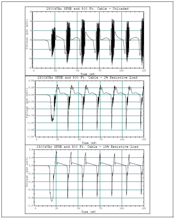
Figure 5 shows a set of three waveforms of the voltage for successively increasing load. The rapid drop in ferroresonant voltage magnitude with the introduction of load is due in large part to the damping of the high frequency portion of the transient. This disappears quickly. The remaining voltage waveform bears a strong resemblance to many of the steady state waveforms reported in the literature.
Figure 6 and Figure 7 show other representative waveforms illustrating the variation of waveforms with transformer size and cable length, respectively.
Figure 5: Effect of Load on the Ferroresonant Voltage Magnitude
Figure 6: Effect of Transformer Size with 100 ft. of Cable.
Figure 7: Effect of Cable Length for a 2500 kVA Transformer.
CONCLUSIONS
From these results and the review of the literature concerning trends in ferroresonance with modern transformer designs, we have concluded that it is likely that ferroresonant activity resulting in voltages exceeding 1.25 per unit will occur during normal phase-by-phase switching events and abnormal failure-related events. Based on what we know about how the system will be designed at this time, it appears that the transformers can become isolated on sufficiently long pieces of cable to cause ferroresonance. The threshold of ferroresonance occurs at approximately 100 ft. of cable.
Grounded wye-wye, 5-legged core transformers are not likely to get into a ferroresonance mode that will result in immediate failure of the transformer or connected cables. In fact, for many cases the voltage will not be high enough to cause utility arresters to operate (although customer arresters may). Therefore, if ferroresonance occurs during a switching operation, no damage would be expected if the operation is completed promptly. The greater danger is with ferroresonance that persists undetected for several minutes or hours. Customer equipment may suffer damage even on brief occurrences.
Although we did not simulate it extensively, many sources indicate that delta-connected transformers can easily achieve voltages exceeding 2.5 per unit. They tend to stay in the higher ferroresonance modes we observed in our simulations of the 5-legged core transformer. This can result is rather rapid failure of equipment and protection should be applied
RECOMMENDATIONS
− Fuse protection should be avoided when the length of cable between the fuse and a ferroresonance-susceptible transformer exceeds about 100 ft. Use three-phase tripping fault interrupters instead. This is similar to the recommendations of other investigators who would suggest critical lengths in the range of 60 to 200 ft for a 2500 kVA transformer.
− Phase-by-phase switching of unloaded transformer when more than 100 ft of cable is involved should be done with the anticipation of ferroresonance.
− Operating procedures should be reviewed in light of the possibility of ferroresonance and revised where necessary.
− Customers with critical loads who may have a desire to dump the utility bus and switch to backup power at the first sign of utility system trouble, should be advised to design their systems to leave significant lighting loads on the utility bus to reduce the chances that the ferroresonance will be damaging.
− Delta-connected transformers should be avoided on the 25-kV system. If present, they should be protected with adequate arresters. If such a transformer is discovered in ferroresonance, it should be de-energized completely for a sufficient time to allow the arresters to cool before re-energization.
REFERENCES
Reinhold Rudenberg, Transient Performance of Electric Power System, MIT Press, May 1970, Chapter 48.
B.A. Mork, D. L. Stuehm, “Application of Nonlinear Dynamics and Chaos to Ferroresonance in Distribution Systems,” IEEE/PES Summer Meeting, Vancouver, 1993, Paper No. 93 SM 415-0 PWRD.
Xusheng Chen, “A Three-phase Multi-legged Transformer Model in ATP using the Directly-formed Inverse Inductance Matrix,” Paper No. 95 SM 421-8 PWRD, IEEE/PES Summer Meeting, Portland, OR, 1995.
D. L. Stuehm, B. A. Mork, D. D. Mairs, “Five-legged Core Transformer Equivalent Circuit,” IEEE Transactions on Power Delivery, Vol 4, No. 3, July 1989.
R. A. Walling, et. al., “Performance of Metal-Oxide Arresters Exposed to Ferroresonance in Padmount Transformers,” IEEE Transactions on Power Delivery, Vol 9., No. 2, April 1994, pp. 788 ff.
RELATED STANDARDS IEEE C57.105-1978
GLOSSARY AND ACRONYMS TNA: Transient Network Analyzer
Published by V. S. Jape#1, D. S. Bankar*2, Tejaswini Sarwade#3 Electrical Engineering1, Electrical Engineering2, Electrical Engineering3, BVDU Pune1, BVDU Pune2, SPPU Pune3 1jape_swati@yahoo.co.in , 2dsbankar@bvucoep.edu.in , 3sarwadet@gmail.com
Abstract— Tracking of system overall performance in phrases of Power Quality disturbances and its ill effects on distribution network is growing attention of application towards tracking of Power Quality indices like voltage sag, voltage swell, and harmonics. The paper introduces new index as Power Quality Distortion Index (DI) which offers the contribution of every load on the total distortion of the power system. Presented system set the basis of tracking and analysis of Power Quality indices for distribution network. The characterization of Power Quality problems is found through non-widespread currents, voltages and frequencies. The Power Quality is related to variations of supply voltage in the form of sags, swells, harmonics, transients, and so on. These troubles outcomes in deterioration of energy deliver to end customers, technology of various disturbances. The loads used by consumers also account for deterioration of Power Quality. Penalties are charged for low power factor loads but at the same time negligence to sizable existence of Power Quality parameters issues like voltage sags and harmonic distortions. Introduction of Custom Power Devices (CPD) is an effective solution over Power Quality problems in distribution network. Paper presents diverse Power Quality indices like Distortion Index as the computational parameter of Power Quality and design of Dynamic Voltage Restorer (DVR) to compensate voltage sag in the system. Effect of DVR on Distortion Index (DI) is also observed and outcomes are analyzed with the assist of MATLAB/SIMULINK.
Keywords — Power Quality, Harmonics, Custom Power Devices (CPD), Dynamic Voltage Restorer (DVR), Distortion Index (DI)
I. INTRODUCTION
The power system layout has become extra complicated every day. It comprises numerous generating stations and loads whose interconnection is through numerous transmission and distribution strains. Also, multiplied use of power electronics based, plc primarily based circuit’s outcomes into growth in nonlinearity. These sorts of loads are sensitive to Power Quality parameters including voltage sags, swells, harmonics, sparkles, fluctuations, etc.
Existence of harmonic distortion is due to deviation in voltage, current or fundamental frequency. The voltage sag is a drop off in root mean square value of voltage or current usually between 0.1 per unit to 0.9 per unit at power frequency lasting for half cycle to 60 seconds. Fault clearing time refers the variety of 3 to 30 cycles [1].voltage swell is rise in root mean square value of voltage at power frequency between 1.1 per unit to 1.8 per unit lasting for half cycle to 60 seconds. Transients are the part of change within the variable disappears in the course of alteration from one consistent state to every other.
II. POWER QUALITY IMPROVEMENT
Enhancement in efficiency of power system desires continuous working which in addition attributes the importance of monitoring for any form of disturbances that’s to be taken into consideration as Power Quality issues and also offer corrective measures on such problems to restrict the occurrences of those events. Mitigation of Power Quality problems is difficult with the aid of the use of traditional equipments including tap changing transformers, lightning arresters, surge arresters, capacitor banks, and many others. Also existence of power electronics devices performs a vital role to decide performance of PQ issues. Power Electronics primarily based solutions are specially categorized as FACTS Controllers for transmission systems and Custom Power Devices (CPDs) which contributes fundamental function in Power Quality improvement of distribution network. Various CPDs are available consisting of Distribution Static Compensators (D-STATCOM), Active Power Filters (APF), Dynamic Voltage Restorer (DVR), Battery Energy Storage Systems (BESS), Static VAr Compensators (SVC), and so on. Dynamic Voltage Restorer (DVR) is identified as more efficient device among of all devices.
A. Control Methods of DVR
Control of DVR circuit topology is critical element for design and modelling factor of view, which includes voltage disturbances identification with proper recognition strategies. Voltage supply converter at once impacts DVR overall performance because it satisfies reactive power requirement. Therefore it is taken into consideration as important a part of DVR [2]. The inverter control strategies are usually categorized as follows:
Fig. 1 DVR Controls
III. MONITORING AND ANALYSIS OF POWER QUALITY PARAMETERS: A CASE STUDY
To analyze the impact of Power Quality parameter, a 11KV/440V, 200KVA substation is considered which supplies power to an educational Institute, The effect on voltage sag, voltage harmonic distortion, current harmonic distortion is observed by using implementing the layout of DVR System in MATLAB/SIMULINK as shown in Fig.3.
DVR is a sequence connected Custom Power Device that’s injected in between distribution network and the load. Basic characteristic of DVR is to inject a required compensation voltage to mitigate Power Quality issues. Nine distinct departments (D1-D9) of the institute are taken into consideration. The overall load linked to the system is 600.68 kW. DVR is connected between supply side and department D2 considering different load conditions.
Table 1 shows System Parameters.
TABLE I SYSTEM PARAMETERS
Fig. 2 Simulink Diagram for Institution with DVR
The DVR subsystem is shown in Fig. 3.
Fig. 3 DVR Subsystem
A. Results
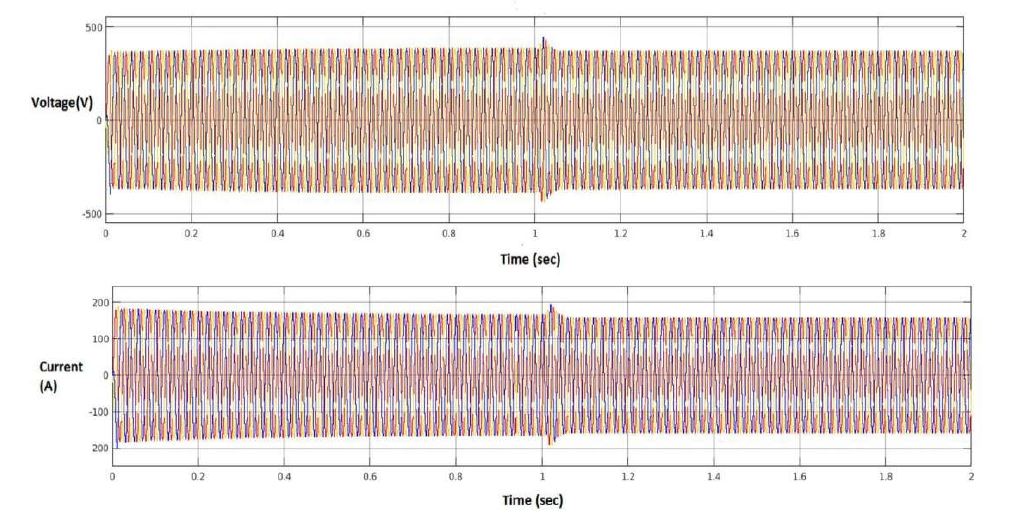
Fig. 4 indicates source voltage waveform wherein voltage sag is observed in among zero- 1 second. The voltage and current waveforms of department in which nonlinear loads are substantial with inclusion of DVR are shown in Fig. 5.
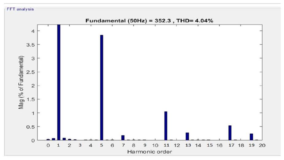
Also, Fig. 6 and 7 indicates voltage THD values earlier than and after DVR connection for a linear and nonlinear load.
Fig. 4 Source Voltage Waveform
Fig. 5 Voltage and Current waveforms for D2
Fig. 6 Voltage THD for non-linear load (before DVR connection)
Fig. 7 Voltage THD for non-linear load (after DVR connection)
THD readings are determined for nonlinear load. Also current THD readings are observed for linear and nonlinear loads before and after DVR implementation inside the system and effects are represented in Table 2.
TABLE II SYSTEM RESULTS
Table 2 indicates the decreased values of THD because of inclusion of DVR in the system. Same results can be observed after connecting DVR in other departments of device with distinct loads.
B. Distortion Index Calculations
Along with THD analysis some other parameter known as Distortion Index (DI) is calculated for the system and is analyzed via simulation. Following formulae are used to calculate DI.
Following formulae are taken into consideration to calculate Distortion Index. Let us consider V1 and I1 be the fundamental voltage and current. V3, V5, V7,…..Vn and I3, I5, I7,……… In are orders of harmonic voltages and currents respectively.
IH = √I32 + I52 + I72 (1) VH = √V32 + V52 + V72 (2) Total Harmonic Distortion Voltage VTHD = VH / V1 (3) Total Harmonic Distortion Current ITHD = IH / I1 (4) Fundamental Apparent Power FAP = V1I1 (5) Current Distortion Power CDP = V1IH (6) Voltage Distortion Power VDP = VHI1 (7) Harmonic Distortion Power HDP = VHIH (8) Non-linear Apparent power NAP = √CDP2 + VDP2 + HDP2 (9) Total Apparent Power TAP = √FAP2 + NAP2 (10) Distortion Index DI = NAP / FAP *100 (11)
Table 3 indicates DI values for departments D1-D9 in the system before DVR connection and after DVR connection.
TABLE III DISTORTION INDEX
Fig. 8 Graphical representation of variation of DI with departments
IV. CONCLUSIONS
From various observations, the outcomes are in comparison. It has been highlighted that the harmonic contents and Distortion Index is reduced significantly with the inclusion of DVR in system. In this regard, a new procedure is presented which evaluates the Distortion Index with DVR and without DVR for non-linear loads connected to the power distribution network.
Contribution of Power Quality Indices is the most important subject to reveal Power Quality stages often. From observations Total Harmonic Distortion displays most effective voltage or the current distortion, while, Distortion Index(DI) pertains to distortion in distribution power. Hence DI can be introduced as main Power Quality index for identification and evaluation of Power Quality levels present inside the distribution network. The regulatory authority can consider this index as “Quality factor” or “Penalty Factor”
ACKNOWLEDGMENT
The research work is being carried out in Bharti Vidyapeeth Deemed University COE, Pune in consent with MSEDCL, Pune. The authors desire to thank authorities of BVDUCOE, Pune for granting permission to publish the work.
REFERENCES
[1] T. Sarwade, V. S. Jape, and D. G. Bharadwaj, “Power quality problems mitigation using dynamic voltage restorer (DVR) using pi controller and fuzzy logic controller,” IJET, vol.2 issue 12, pp. 214-218, Apr. 2018. [2] C. H. Raval, and A. Doorwar, “An Overview of Various Control Methods of DVR,” in ICCPCT, 2014, p. 53 [3] R. Omar, and N. A. Rahim, “Implementation and Control of a Dynamic Voltage Restorer using Space Vector Pulse Width Modulation (SVPWM) for Voltage sag Mitigation,” in IEEE-TECHPOS, 2009, p. 1. [4] V. S. Jape, and D. G. Bharadwaj, “Substation Monitoring System (SMS) For Remote Power Quality Monitoring and analysis of Power Distribution Network using Object Oriented Web Enabled Method,” IJCTA(International Science Press), 10(9), pp. 533- 539, 2017. [5] R. C. Dugan, and M. F. McGranghan, Electrical Power System Quality, Tata McGraw Hill, 2nd Edition. [6] S. Vlahinic, D. Brnobic, and N. Stojkovic, “Indices for harmonic Distortion Monitoring of Power Distribution Systems,” Instrumentation, pp. 12-15, 2008. [7] IEEE Recommended Practices and Requirements for Harmonic Control in electrical Power Systems, IEEE Std 519-1992. [8] IEEE Recommended practice for monitoring electric power quality, IEEE STD 1159-1995.
Source: JASC: Journal of Applied Science and Computations, ISSN NO: 1076-5131, Volume 5, Issue 10, October/2018
Published by Electrotek Concepts, Inc., PQSoft Case Study: Distribution Feeder Energizing, Document ID: PQS0711, Date: October 15, 2007.
Abstract: The energization transients for distribution feeders are generally a combination of line energizing, transformer inrush, and load inrush. Line energizing transients typically decay to negligible values in about one-half cycle and they generally do not pose significant problems for customer equipment. Energizing a distribution circuit can create a transient overvoltage similar to that generated by a capacitor bank energizing.
This case study presents a feeder energizing evaluation for a 34.5kV distribution system.
INTRODUCTION
A feeder energizing evaluation was completed for the 34.5kV distribution system shown in Figure 1.
Figure 1 – Oneline Diagram for Distribution Feeder Energizing
BACKGROUND
The energization transients for distribution feeders are generally a combination of line energizing, transformer inrush, and load inrush. Line energizing transients typically decay to negligible values in about ½ cycle and they generally do not pose significant problems for customer equipment.
Energizing a distribution circuit (e.g., lines and/or cables) can create a transient overvoltage similar to that generated by a capacitor bank energizing. Transients generated by energizing overhead distribution lines are characterized by high frequencies (e.g., 2-10 kHz) because of the small effective shunt capacitance (e.g., 15 ηF/mile) of these circuits. These high frequencies are quickly attenuated by the distribution line resistance and circuit loads. Long cable circuits have higher capacitance (500-1000 ηF/mile) and can look similar to capacitor banks when they are energized. This means that the characteristic frequencies are lower (e.g., 500-2000 Hz) and the transients can last longer. If the distribution circuits include capacitor banks, the energizing transients will be dominated by the capacitor banks and the associated frequencies will be lower (e.g., 300-800 Hz).
Besides, the effect of the line or cable capacitance, energizing transmission lines also causes traveling waves that appear as high frequency transients. Traveling waves are caused by the distributed nature of the capacitance and inductance of the transmission or distribution line. These transients are damped by circuit resistance and load on the power system but can be a concern during light load conditions. The frequencies are high enough (natural frequencies of distribution circuits without shunt capacitors are in the range 1-10 kHz) that these transients can be coupled to secondary circuits by the capacitance ratio of step-down transformers.
Figure 2 shows an example measured voltage waveform on a 12.5kV feeder during reclosing after clearing a fault on the feeder.
Figure 2 – Example Distribution Feeder Energizing Voltage Waveform
Figure 3 shows an example measured three-phase voltage waveform on a 13.8kV substation bus during energization of a distribution feeder. The worst-case transient voltage was approximately 1.71 per-unit (171%).
Figure 3 – Example Distribution Feeder Energizing Voltage Waveform
SIMULATION RESULTS
The accuracy of the system model was verified using three-phase and single-line-to-ground fault currents and other steady-state quantities, such as transformer and induction motor rated currents. The distribution circuit model has two branches, each approximately 6000-7000 feet in length. Customer loads are distributed along the entire length of the feeder, with three of customer transformers also supplying 300 hp induction motors. Several 2,400 kVAr capacitor banks are placed along the feeder to maintain a reasonably constant steady-state voltage profile. The customer transformers are modeled using a five-legged core design.
The lengths of the cable segments were 1,000 feet. The cable size was 600 MCM with the following characteristics:
Insulation:……………………………….0.1406 outside diameter in feet Jacket:……………………………………0.1412 outside diameter in feet Neutral:…………………………………..0.1409 outside diameter in feet
A line constant program was used to compute the positive and zero-sequence impedances of the cable, yielding the following results:
Z1 = 0.0231 + j 0.0824 ohms/1000 ft Z0 = 0.1828 + j 0.6854 ohms/1000 ft C1 = C0 = 78.24 ηF/1000 ft
The initial case (Case 3a) involved energizing the 34.5kV distribution feeder by closing the circuit breaker B1 with all of the customer load and capacitor banks in-service. Figure 4 shows the three-phase bus voltage at the 34.5kV substation bus when the circuit breaker B1 is closed. Figure 5 shows the corresponding 34.5kV feeder inrush current.
Figure 6 shows the results of a Fourier analysis of the current waveform. The highest harmonic current components are between the 2nd and 7th harmonics, which correspond to the characteristic frequencies for load, transformer, and capacitor bank energizing transients.
Figure 4 – Simulated Distribution Feeder Energizing Voltage
Figure 5 – Simulated Distribution Feeder Energizing Current
Figure 6 – Simulated Distribution Feeder Energizing Current Harmonic Spectrum
The second case (Case 3b) shows the effect of a short duration fault and circuit breaker reclosing on the feeder voltage waveform. Figure 7 shows the three-phase voltage near the end of one branch of the 34.5kV distribution feeder during a six-cycle fault at the end of the feeder.
Figure 7 – Simulated Distribution Feeder Voltage during a Short Duration Fault
CONCLUSIONS
Observations and conclusions for this case study include:
Distribution feeders energizing transients are generally a combination of line energizing, transformer inrush, and load inrush transient characteristics.
Long distribution cable circuits have relatively high capacitance (500-1000 ηF/mile) and can look similar to capacitor banks when they are energized. This means that the characteristic frequencies are relatively low (e.g., 500-2000 Hz) and the transients can last significantly longer.
For distribution circuits that include capacitor banks, the energizing transients will be dominated by the capacitor banks and the associated frequencies will be approximately 300-800 Hz.
Distribution feeder energizing transients typically decay to negligible values in about ½ cycle and they generally do not pose significant problems for customer equipment. Excessive transient overvoltages will likely be limited by arresters installed on substation and feeder equipment.
RELATED STANDARDS IEEE Std. 1036
GLOSSARY AND ACRONYMS MOV: Metal Oxide Varistor Arrester MSSPL: Maximum Switching Surge Protective Level SiC: Silicon Carbide Arrester
Published by Electrotek Concepts, Inc., PQSoft Case Study: Voltage Sag Study – Application of a Static Transfer Switch, Document ID: PQS0317, Date: July 18, 2003.
Abstract: The purpose of this case study is to determine the feasibility of reducing process equipment disruptions due to utility voltage sags at a large industrial facility. The facility consists of many injection molding machines, resulting in an industrial process that is extremely sensitive to distribution voltage variations. The case study investigates various distribution system modifications to determine the most effective and efficient means for providing the level of power quality necessary for proper plant operation.
INTRODUCTION
The purpose of this study is to determine the feasibility of reducing process equipment disruptions due to utility voltage sags at a large industrial facility. The study focuses on necessary modifications to the utility distribution system.
The plant manufactures plastic cases for automobile batteries and is served by 480-V, three-phase, four-wire. The plastics plant operates 24/7, peaks at about 1000 kW, and has an annual electricity cost of approximately $347,000. The customer has not reported the magnitude of dollar losses associated with voltage sags, nor have they provided log information about the number of disturbances suffered and the specific equipment affected. In addition, the customer has insisted that the voltage sag problem be solved on the utility system, rather than inside the plant. The manufacturer says they are not unwilling to modify the existing injection molding machines to provide selective ride-through, nor does it want to bear the expense of providing ride-through equipment capable of protecting entire machines.
Customer Equipment and Utility Supply Description
Injection Molding Machines
The plant operates 19 injection molding machines and two automatic assemblers. Each machine consists of an ac hydraulic pump motor, a dc extruder motor, and electronic controls and robotics. The total connected molding machine load is about 2000 kW. Plant billing demand is about 1000 kW, but is soon to increase with the addition of ten machines. The plant is highly automated and requires only 7 operating personnel. The few operators make for difficult recovery when production upsets occur. The typical voltage sag disrupts the computer controls serving robotics and causes drop-out of magnetic contactors for the hydraulic pumps.
Summary
The plant is served from Delivery #3 (Del#3), a transmission-to-distribution substation. The substation is fed from the local utility’s 100 kV transmission system. The plant’s 23 kV feeder is designated as Circuit 332 and is shown schematically in Figure 1. Del#3 also serves three other 23 kV distribution feeders, 333, 334, and 335. The local utility operates two similar points-of-delivery, designated as Delivery #1 (Del#1) and Delivery #2 (Del#2). Circuit #112, from Del#1, is being considered as the source of an alternate 23 kV feed to the plant because it will be extended to the vicinity of the customer’s site to accommodate system improvement and load growth requirements.
Figure 1 Existing Utility’s Electrical Distribution System
The city should expect one to two feeder breaker operations per month per feeder on its 23 kV distribution system. Based on Electrotek’s experience, this level of activity is typical for overhead distribution systems with multiple feeders per substation with the kind of animal, vegetation and lightning exposure which exists in the area. Standard construction, multiple feeder per substation, overhead distribution circuits are not designed to provide the type of performance required by sensitive industrial customers like the one here.
Utility-Side Solution to Voltage Sag Disturbances
Table 1 summarizes the utility-side options for reducing voltage sag interruptions at the plant. The table is arranged with the present service (Feeder #332 out of Del#3) listed first, and the other service options listed in order of decreasing interruptions at the customer’s site. This table is based upon the utility’s SCADA information and utilizes several assumptions (outlined in Table 1). The most important of these assumptions is that the table is based on one test year of interruption data. Fault data in other years may be considerably different. The table also does not include sags due to faults on the transmission system.
Table 1 Utility-Side Options for Improving Service at the Customer’s Site
Table 1
Recommended Solution — Dual Feed and Static Transfer Switch
Electrotek recommends that the utility install a dual-feed service to the plant which includes an electronic static transfer switch, as shown schematically in Figure 2. This service will dramatically reduce the number of interruptions to the plant, and can be integrated into the utility’s load growth plans to relieve some of the installed cost of the system. Preliminary estimates indicate that the new service can be installed for about $300,000, not including the costs to extend Circuit #112 to the site.
Table 2 shows a breakdown of the estimated costs.
Table 2 Breakdown of Costs to Install Static Transfer Switch and Monitor Performance
Table 2
Figure 2 Proposed Dual-Feed Service to Plant with Static Transfer Switch
Operating costs for the static transfer switch are expected to be minimal. The manufacturer lists the switch efficiency at 99.5%. Power losses in the switch therefore will add less than $5000 to the customer’s annual billing. Similar static transfer switch installations have not been air conditioned, so the additional energy costs related to the switch will be limited to ventilation fan operation. The electronic components require little maintenance.
Static Transfer Switch
The electronic static transfer switch consists of silicon-controlled rectifiers (SCR’s) which can quickly disconnect sensitive loads from a preferred source, and re-connect the loads to an un-faulted alternate source. At the plant, the preferred source would be the new 2500 kVA padmount transformer served from Circuit #112, while the alternate source would be the existing service. The static transfer switch can transfer to the alternate source in approximately ¼ to ½ cycles.
The static transfer switch will transfer to the alternate source under the following conditions:
Source undervoltage (less than about 80% on any single phase);
Source overvoltage (greater than 110%);
Loss of continuity in source-side SCR (SCR failure);
Blown fuse in source;
Manual signal.
It is designed to transfer back to the preferred source when:
The preferred source is in-phase;
The preferred source is within 10% of nominal voltage for greater than 2 sec (adjustable);
Operator switch is in “automatic” position;
The transfer to alternate was not caused by an SCR failure.
Electrotek expects that the switch will alleviate the majority of voltage sags which cause an adverse impact to plastics plant. The plant will still be susceptible to deep sags on the utility’s transmission system, distribution system faults which affect Del#1 and Del#3 simultaneously, and failures in the static transfer switch itself. These occasions are expected to be rare.
SUMMARY
Electrotek recommends that the utility combine planned system improvements with modifications in its service to the plastics plant to lessen the plant’s exposure to voltage sags. The proposed project would include splitting the Del#1 23 kV bus, extending Circuit #112 to the customer’s site, installing a new 2500 kVA transformer to accommodate additional load growth within the customer’s facility, and installing an electronic static transfer switch capable of transferring the plant load to Circuit #332 during interruptions and voltage sags on Circuit #112. Electrotek estimates that the static transfer switch will add approximately $300,000 to the system improvement project.
Modifications to a utility system which benefit a single customer are generally paid for by that customer. Normal utility practice is to apply additional facilities charges to the customer’s monthly electric bill to cover the cost of the improvements. These monthly charges generally equal 1.0% to 2.0% of the installed cost of the improvements and apply indefinitely. The utility uses a plan which applies a monthly charge of 1.7%. The additional facilities charge under this plan would add less than 10% to the customer’s projected monthly billing after the expansion.
The plastics manufacturer could realize a significant reduction in economic losses associated with voltage sags by accepting the static transfer switch solution. These savings could be applied against the additional facilities charges. In addition, the customer’s load growth may qualify the plant to receive an economic development incentive rate. The incentive rate savings, by utility calculations, could exceed $150,000 over the next five years. These savings would also lessen the impact of the facilities charges.
REFERENCES
Static Transfer Switch Primer, EPRI, Palo Alto, CA, 1998, TR-111697. Banerjee, B., Smith, J., The Static Transfer Switch: Current Technologies, Operation, and System Requirements, PQA ’99, Charlotte, North Carolina, May 1999.
GLOSSARY AND ACRONYMS Voltage Sag: A decrease to between 0.1 and 0.9 pu in rms voltage or current at the power frequency for durations from 0.5 cycles to 1 minute.