Published by Electrotek Concepts, Inc., PQSoft Case Study: Feeder Lightning Transients, Document ID: PQS1101, Date: March 15, 2011.
Abstract: Lightning strokes to exposed utility transmission or distribution circuits can inject a significant amount of energy into the power system in a very short time, causing deviations in voltages and currents which persist until the excess energy is absorbed by dissipative elements (e.g., arresters). This case study presents a distribution feeder lightning transient overvoltage evaluation.
FEEDER LIGHTNING TRANSIENT CASE STUDY
A utility distribution system lightning transient analysis case study was completed for the system shown in Figure 1. The case study investigated the potential for severe high frequency transient overvoltages on distribution feeder primary and customer secondary buses during a lightning strike on the feeder primary. The power conditioning mitigation alternative of MOV surge arresters was also evaluated.
The simulations for the case study were completed using the PSCAD® program. A high-frequency transient model was created to simulate the lightning transients and resulting overvoltages and arrester energy duties. A high-frequency model was required to accurately represent the very high lightning transient frequencies. The lightning surge was assumed to be a current source with a very fast rise time (e.g., 8×20μsec).
The modeled circuit consisted of a 138 kV utility substation supplying a 50 MVA, 138kV/34.5kV substation transformer. A high frequency, distributed parameter transmission line model was required to accurately represent the traveling wave (reflections) effects during the lightning transient. Two 34.5 kV distribution feeders were included in the model. The first feeder consisted of 5-mile and 15-mile overhead feeder segments that were modeling using the distributed parameter transmission line model. The second feeder included 3-mile and 9-mile underground cable segments that were modeled using the frequency dependent cable model. Both line and cable constants were determined and the data was used to help validate the system model.
Traditional inductive transformer models generally look like an open circuit to the very high frequency lightning transients. Therefore, the 60 Hz transformer model can be improved by adding capacitances between windings and from the windings to ground. This type of model will act as a capacitive voltage divider to transfer a portion of the surge from the primary to the secondary windings. Bushing and winding capacitance values for the substation and customer step-down transformers were assumed based on typical data. Other substation equipment, such as circuit breakers and instrument transformers, are represented by their stray capacitances to ground. Typical stray capacitance values of substation equipment are provided in Annex B of IEEE Std. C37.011.
Figure 1 – Illustration of Oneline Diagram for Lightning Transient Overvoltage Evaluation
Lightning is a weather-related phenomenon that is often thought to be the principal cause of most high frequency transients. Energy from lightning strokes may enter the power system in several ways. A direct stroke to exposed equipment (e.g., overhead distribution feeder) is the most obvious. Because of the high-frequency and high-energy associated with a lightning flash, it is also possible for significant energy to be coupled into the power system from indirect strokes as well. Finally, in situations where more than one ground reference exists, it is possible for the potential difference generated by conduction of stroke current to ground to be conductively coupled into equipment. This can be especially important for computer and communications equipment.
Susceptibility of the power system to lightning is best characterized statistically, since the occurrence rate and stroke current magnitudes of lightning ground flashes is otherwise impossible to predict. Based on years of observations, the incidence of cloud-to-ground lightning flashes has been related to the level of thunderstorm activity, or isokeraunic level, in a general region. Magnitudes of lightning stroke currents range from 2 kA to 200 kA, although the probability of very small or very large magnitude is low. The average lightning surge current is approximately 30 kA.
When lightning strikes a portion of the power system directly, a voltage impulse equal to the product of the stroke current and the equivalent surge impedance of the power system will be created. The surge will propagate in all directions on the power system, dividing amongst all available paths at terminations. Energy may also be coupled into circuits that are not directly connected to the stricken system. The rapid rate-of-rise and high magnitude impulse will result in operation of surge arresters or flashover of line or equipment insulation. The high energy associated with a direct strike to the power system can easily exceed the withstand capability of surge arresters or other protective devices since they are not designed for this severe contingency.
Transient surges coupled into the power system from indirect strokes will propagate in a similar manner. While utility system protective equipment will operate properly and be able to withstand such an occurrence, there are mechanisms by which the effects of the indirect stroke can affect customer utilization equipment. High currents diverted into the grounding system by surge arresters will raise the potential of a local ground grid well above that of “true earth.” This “ground potential rise” (GPR) is of no consequence for equipment referenced only to the affected grid; there are situations however, where connections to remote ground references can result in misoperation or equipment damage under these conditions. Shielded communications and data circuits may be especially susceptible. Circuits connecting nearby buildings may be exposed to GPR should the building ground grids be separated electrically and one of them is struck by lightning. Under these conditions, an “isolated” computer ground can be a source of damaging or even lethal voltages and for this reason should never be used.
When evaluating these disturbances, it is important to remember that the stress on equipment is based on the impulse magnitude and duration plus the magnitude of the fundamental component at the instant of the impulse. The most common cause of impulsive transients is lightning. Due to the high frequencies involved, impulsive transients are generally damped quickly by resistive components in the circuit (e.g., conductor and transformer resistance). These transients are most prevalent very close to the disturbance that causes the transient (e.g., lightning, switching event, etc.) and there can be significant differences in the transient characteristic from one location within a facility to another.
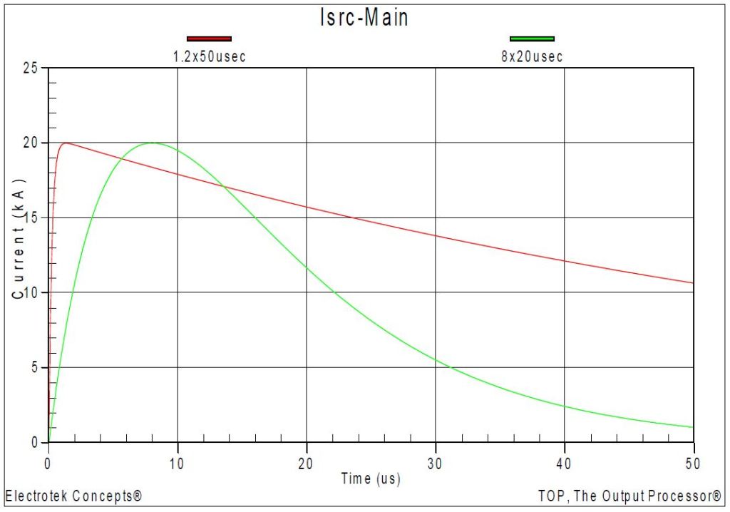
Figure 2 shows two representative lightning current waveforms commonly used in transient simulation studies. The figure shows a 20 kA—1.2×50 μsec and a 20 kA—8×20 μsec lightning stoke current characteristic. The simulation was completed using the PSCAD program.
Figure 2 – Example Representative Lightning Current Waveform
The first simulation (Case 1) case involved a lightning strike to the 34.5kV feeder #1 at the Customer #1 primary bus (Phase A) with no MOV arresters included in the model. The specifications of the lightning current waveform were a 10 kA magnitude and an 8×20 μsec characteristic. The simulated lightning current waveform is shown in Figure 3.
Figure 4 shows the resulting feeder primary voltage for Case 1. The peak transient voltage with no arresters included in the model was 243.7 kV. The waveform illustrates voltage reflections from the ends of the overhead feeder and underground cable segments. Figure 5 shows the corresponding substation bus voltage, which has a peak voltage magnitude of 192.5 kV and Figure 6 shows the Customer #1 secondary bus voltage, which has a peak voltage of 3212.9 V.
A 27 kV MOV arrester was included on the primary winding of the Customer #1 transformer for Case 2. The assumed ratings for the arrester included:
Rated Voltage (Duty Cycle): 27 kV Maximum Continuous Operating Voltage (MCOV): 24.4 kV Maximum Energy Discharge Capability: 2.0 kJ/kVrated MCOV Maximum Energy Discharge Capability: 48.8 kJ 10kA, 8×20μsec Discharge Voltage: 73.1 kV
Figure 3 – Lightning Surge Current Waveform for Case 1
Figure 4 – Feeder Primary Voltage Waveform for Case 1
Figure 5 – Substation Bus Voltage Waveform for Case 1
Figure 6 – Customer Secondary Bus Voltage Waveform for Case 1
Case 2 involved a lightning strike to the 34.5kV feeder #1 at the Customer #1 primary bus with the 27 kV MOV arrester included in the model. Figure 7 shows the resulting feeder primary voltage. The peak transient voltage with the arrester included in the model was 70.1 kV, which was approximately equal to the arrester’s 10 kA discharge voltage.
The simulated arrester energy duty was 8.0 kJ, which was approximately 16% of the assumed energy capability. Figure 8 shows the corresponding Customer #1 secondary bus voltage, which has a peak voltage of 961.5 V.
A low voltage surge arrester was included on the secondary winding of the Customer #1 transformer for Case 3. The assumed ratings for the arrester included:
Rated Voltage (Duty Cycle): 277 V Maximum Continuous Operating Voltage (MCOV): 305 V Maximum Energy Discharge Capability: 2,200 J 10kA, 8×20μsec Discharge Voltage: 910 V
Case 3 involved a lightning strike to the 34.5kV feeder #1 at the Customer #1 primary bus with both the primary and secondary arresters included in the model.
Figure 9 shows the resulting feeder primary voltage. The peak transient voltage with the primary arrester included in the model was 70.1 kV. Figure 10 shows the corresponding Customer #1 secondary bus voltage with the secondary arrester included in the model. The peak voltage was reduced from 961.5 V to 672.8 V. The energy duty for the secondary arrester was less than 10 J.
Figure 7 – Feeder Primary Voltage Waveform for Case 2
Figure 8 – Customer Secondary Bus Voltage Waveform for Case 2
Figure 9 – Feeder Primary Voltage Waveform for Case 3
Figure 10 – Customer Secondary Bus Voltage Waveform for Case 3
SUMMARY
This case study summarized a distribution feeder lightning transient overvoltage evaluation. A high-frequency transient model was created to simulate the lightning transients and resulting overvoltages and arrester energy duties. A high-frequency model was required to accurately represent the lightning phenomena. Surge arresters were evaluated as the power conditioning alternative.
REFERENCES
“IEEE Recommended Practice for Monitoring Electric Power Quality,” IEEE Std. 1159-2009, IEEE, June 2009, ISBN: 978-0-7381-5940-9.
“IEEE Application Guide for Transient Recovery Voltage for AC High Voltage Circuit Breakers Rated on a Symmetrical Current Basis,” IEEE Std. C37.011-1994, IEEE, ISBN: 1 55937-467-5.
“Electrical Transients in Power Systems,” Allan Greenwood, Wiley-Interscience; Second Edition, April 18, 1991, ISBN: 0471620580.
R.C. Dugan, M.F. McGranaghan, S. Santoso, H.W. Beaty, “Electrical Power Systems Quality,” McGraw-Hill Companies, Inc., November 2002, ISBN 0-07-138622-X.
RELATED STANDARDS IEEE Std. 1159, IEEE Std. C37.011
GLOSSARY AND ACRONYMS ASD: Adjustable-Speed Drive CF: Crest Factor DPF: Displacement Power Factor PF: Power Factor PWM: Pulse Width Modulation THD: Total Harmonic Distortion TPF: True Power Factor
Published by Tadeusz GLINKA1,2, Marek GLINKA2 Politechnika Śląska w Gliwicach (1), BOBRME Komel (2)
Abstract. Design of steel-plant furnace three-phase transformer (110 kV/(350 to 500) V, 50 kA) and its operating conditions are described in the paper. After three months of operation this transformer failed. Cause of failure, its course and damage to transformer winding are presented. Recommendations for transformer winding design and its installation and protection are given.
Streszczenie. W artykule opisano budowę trójfazowego transformatora piecowego 110 kV/(350 do 500) V, 50 kA i warunki jego pracy w miejscu zainstalowania. Transformator, po trzech miesiącach pracy, uległ awarii. Opisano przyczynę awarii, jej przebieg i uszkodzenie uzwojenia transformatora. Podano zalecenia dotyczące wykonania uzwojenia transformatora i zalecenia dotyczące jego zainstalowania i zabezpieczenia. (Problemy eksploatacyjne transformatora hutniczego).
Steel plant transformers are electrical devices providing electrical energy needed in the manufacturing process. The processing requires current control and this is achieved by voltage control (regulation). Usually this is a step voltage control. The necessity of continuous voltage control, that is controlling output voltage when transformer is on load, is a feature distinguishing steel plant transformers design from power engineering transformers (unit and distribution transformers). In case of power engineering transformers, service manuals have been elaborated [1]. The current paper describes a steel plant transformer used to heat liquid steel in the continuous casting processing line. Here the converter’s liquid steel is reheated and ameliorated in ladle arc furnace of 300 Mg holding capacity. The furnace is supplied from two transformers, the main transformer (#1) and booster transformer (#2) connected as shown in Figure
Transformers are placed in a common tank and they constitute one supply circuit with step-controlled voltage. The ratings are as follows: power: (40 000 ÷ 26 327) kVA; primary winding W1: 110 kV; (209,9 ÷ 138,2) A; control windings W2-W3: 15238 V; / (840 ÷ 754) A; secondary winding W4: (514 ÷ 304) V; /(44,9 ÷ 50) kA. The primary winding (W1, marked as high tension voltage GN) of transformer #1 is star-connected and supplied from 110 kV distribution substation by a cable line c. 3 kms long. The distribution substation bus voltage is stepped up and equal to 119 kV. Large power synchronous machines operate in the plant so that the network is overcompensated.
Transformer bay in distribution substation is equipped with a circuit breaker (WS1), disconnector and surge limiters. The secondary winding (W4, marked as DN – low tension voltage) embraces both columns of transformers #1 and #2 and is delta-connected; it is carried outside transformer chamber via bus and connected to furnace electrodes with bundles of elastic wires. Voltage control is achieved with the help of medium voltage winding (winding W2), which is placed in transformer #1 core. Winding W2 is equipped with taps connected with on-load tap changer. There are 13 taps. The control winding W2 supplies the primary winding W3 of booster transformer #2. W2 and W3 windings are star-connected; the neutral points of both star arrangements are connected and earthed via 17 Ω resistance.
The short-circuit voltage between winding W1 (high tension) and winding W4 (low tension) for tap #1 (output voltage 304 V) is equal to 10.93 %, while for tap # 13 (output voltage 514 V) is equal to 7.46 %. The circuit breaker switch (Q1) in medium voltage circuit connects control winding W2 of main transformer (#1) and primary winding W3 of booster transformer (#2). Surge limiters are installed at both sides of Q1 circuit breaker switch. Contactors rated at 1200 A are used as short-circuiting switches 3KM and 4KM of low tension winding W4. They are placed in transformer chamber. The QW short-circuiting switch is a remotely-operated disconnector and is placed outside the transformer chamber.
Fig. 1. Electrical scheme of furnace transformer circuit
W4 winding output terminals and short-circuiting switches 3KM, 4KM and QW are connected by 4 meters long copper cable of 95 mm2 crossection. This cable runs over transformer tank. Transformer and accompanying devices are placed in a brick chamber in plant manufacturing house.
During normal operation of ladle furnace, the QS1 breaker is closed, the circuit breaker Q1 is closed, and the short-circuiting switches 3KM, 4KM and QW are open. Furnace electrodes current control is accomplished by tap changer present in transformer tank. The switch-over of the transformer from normal (on-load) operation to idle run (no-load) is conducted in accordance with following sequence of events:
Q1 circuit breaker is tripped (opened); this causes decrease in load and electrode arc goes out, since booster transformer 2 is not supplied and its secondary winding W4 acts as a reactor with a large inductance,
electrodes are automatically raised,
contactor 3KM is closed and this causes short-circuiting and earthing of DN circuit via resistors R = 1.6 Ω; short circuit state lasts for 3 seconds,
contactor 4 KM is closed, which causes direct short-circuiting and earthing of DN circuit, 3 KM contactor is opened,
if necessary, disconnector QW is closed; this is done by the servicemen eg. when electrodes are lengthened or if current paths connecting DN winding with the electrodes are subjected to maintenance.
Disconnector QW, which doubles the function of short-circuiting switch 4KM is located outside the transformer chamber, since for safety reasons the servicemen must be able to observe the condition of disconnector knife contacts and to make sure that the current path is earthed; only then the maintenance can be performed.
The switchover to ladle transformer normal operation is done by opening the short-circuiting switches QW and 4KM, switching the circuit breaker switch Q1 on and lowering the electrodes until the electric arc is started. The power switch QS1 is coupled via auxiliary contacts with circuit breaker Q1 so that they are interlocked. The circuit breaker Q1 is in turn coupled via auxiliary contacts with short-circuiting switches 3KM, 4KM i QW; this coupling prevents switching Q1 on if DN circuit is short-circuited.
Transformer failure
The investigated transformer was brand new when it was installed and put into operation in July. The failure occurred in October, so it operated only three months. The failure took place during switching the transformer from no-load state to on-load operation. When switch Q1 was closed, emergency cut-off took place, via power switch Q1 installed on the switchboard. The QS1 switch was tripped after 70 ms has passed. The gas-filled protection was also actuated (this breaker constituted the second stage of transformer protection) as well as protections on both medium tension (SN) windings. The surge limiters installed at both sides of Q1 breaker did not operate. The short-circuiting switch 4KM was on and cable connecting low tension winding (DN) with the short-circuiting switch was burned out (gone). The transformer operated in shorted circuit. The bushing insulators were burned and completely damaged by electric arc.
Fig. 2. View of transformer tank cover; locations of bushing insulators and arcing faults are marked
Electric arc occurred between insulators 3A – 2B and 3B – 2C, as shown in Figure 2. Traces of burning by electric arc were also observed at DN winding leads. This arc caused three-phase arcing fault of main transformer SN winding. The measurements conducted sometime after the failure showed that main transformer SN winding had been damaged. The chromatographic tests of gases dissolved in transformer oil and gases obtained from gas-flow relay showed existence of internal short-circuit in the transformer.
Transformer was then moved to the plant where it had been manufactured. When it was taken out of the tank and partially disassembled the following observations were made:
high tension (110 kV) W1 winding had not been damaged,
medium tension (SN) W2 winding of main transformer had been damaged by electrodynamic forces,
medium tension (SN) W3 winding of booster transformer had not been damaged,
low tension (DN) W4 windings of both transformers had
not been damaged
Description of W2 winding damage
W2 winding consists of two layers. The first layer lies immediately next to transformer’s core and is a reversible control winding with 6 taps. The second layer is the basic medium tension winding SN. In phases A B and C the basic winding was pushed up and the control winding down, by 8 to 15 centimetres. Moulding rings made of Elkon transformer plywood broke into several parts and screws keeping the winding in place were driven into the Elkon rings and bent. As a result of insulation layers shift the insulation was locally damaged. Short-circuiting of control circuit (one tapping step) occurred in phases A and B in the very locations where insulation had locally failed. Short-circuiting sites showed small insulation burn-outs and copper melting.
Why did failure occur?
The interlocking between circuit-breaker Q1 and short-circuiting switch 4KM were set up with help of auxiliary contacts. When auxiliary contacts of 4KM switch were closed, then they blocked tripping (switching on) of Q1 circuit breaker and vice versa. Dust with insulating properties is produced and emitted during continuous casting process. The transformer chamber was not air-tight. Dust was able to get into the chamber and, since electrical devices operating in the chamber were live, the chamber was never cleaned. Dust was deposited on auxiliary contacts of 4KM short-circuiting switch and, in time, the contacts became isolated and did not block Q1 circuit switch. Therefore when the short-circuiting switch 4KM was on, the circuit breaker Q1 could have been switched on likewise. Transformer tank cover, the bushing insulators and the wires were all coated with dust. When circuit breaker Q1 was switched on and lower tension winding DN was short-circuited, the electrodynamic forces generated by short-circuit current were such, that the transformer cover was dislodged and the dust cloud rose into air. The short-circuit current at DN side was calculated to be equal to c. 230 kA and current density in short-circuiting cable was equal to c. 2400 A/mm2. With this current density, the copper wire melted after c. 50 ms; between the ends of burned wire electric arc was generated and this caused copper evaporation. Electrodynamic forces present in the arc ejected the copper particles onto the DN winding terminals and to SN bushings. The space between bushings became conductive and this led to arc-type short-circuit between insulators 3A-2B i 3B-2C as shown in Figure 2. This is a short-circuit of main transformer (transformer #1), and this transformer’s short-circuit rated voltage is very small. The short-circuit current rose, and electrodynamic forces generated in the windings increased in proportion to squared current value. The main transformer was not designed to withstand this type of short-circuit.
What errors were committed?
After analysing transformer operating conditions, transformer’s suitability to supply voltage and its design, we get the impression that several undesirable events took place at the same time. These events can be enumerated as follows:
errors in transformer design assumptions,
design and construction defects,
and the greatest errors, which constituted direct cause of failure: transformer’s operating conditions and the setup of contactors’ interlocking.
Transformer design data
The primary (high tension) winding was designed for rated voltage equal to 110 kV. The supply voltage was 199 kV, that is 8.2% higher than rated voltage; hence the short-circuit current went up by 8.2% as well and the electrodynamic forces generated in winding rose by 17%. The second error related to transformer chamber and its lack of dust-tightness. The plant manufacturing house, where continuous casting processing line is located, is full of dust created during manufacturing processes. This dust freely flowed into transformer chamber, mainly through ventilation ducts and deposited itself on all devices present inside the chamber. Electrical devices operating in the chamber were live, so that the chamber was never cleaned and dust not removed.
Transformer design and construction defects
The control winding W2 has been designed with taps. When tap is connected into the circuit, only part of the winding operates and it is placed non-symmetrically in the column in relation to primary winding W1 (Fig. 3). This asymmetry is particularly significant in case of tap No.1. This tap was connected during the investigated short-circuit event.
During second stage of short-circuit, the ampere turns of W1 and W2 windings were equal to each other, this may be concluded from theory of transformers [2,3]. The said asymmetry generates magnetic fields in transformer window: longitudinal field By and transverse field Bx, The interaction of these fields and windings current produces electrodynamic forces, this is shown in Figure 3. Figure 3 is of course only a model illustrating generation of forces Fx i Fy, and in particular axial force Fy which became the destructive force. The Fy might be smaller if the active part of W2 control winding at each tap was distributed uniformly along the column height, since the Bx flux density component is then minimum (see Fig. 4).
Fig. 3. Active parts of transformer #1 (marked) during the short-circuit-event; directions of electrodynamic forces are shown and distribution of flux density in transformer window
Errors in control and protection circuit
The biggest error and the direct cause of the failure was a mistake made during the design of control and protection circuits. The interlocking of circuit breaker Q1 and short-circuiting stitch 4KM was prone to failure. The other error was placing of short-circuiting switch 4 KM directly in transformer chamber and locating the earthing cable (from W4 terminals to 4KM switch) on the transformer tank surface.
Fig. 4. Correct execution of transformer #1 control winding
Conclusions
Transformer failure has been analysed thoroughly and in detail by experts. Their recommendations were:
to set up second interlocking between circuit breakers Q1 and 4KM, eg. based on current measurements in holding coils of Q1 and 4KM breakers (obligatory measure),
to connect earthing cable to DN (low tension) current cables outside the chamber; short-circuiting switches 3KM and 4KM should be installed outside the chamber (obligatory measure),
high tension winding W1 should be manufactured for rated voltage equal to 120 kV,
taps of control winding W2 should be distributed along the column height (as shown in Fig. 4); the clamping of moulding Elkon rings should be changed from pointwise to surface-wise; the ring holding should be strengthened (thickened),
transformer chamber should be sealed, air-blast should be introduced and chamber pressure kept at all times above the ambient (manufacturing room) pressure (obligatory measure).
Transformer after overhauling has been operating without further failure for 15 years.
The question arises whether investor of continuous casting processing line should had got experts’ opinion on line design before it was erected. Was failure (and resultant high repair costs) necessary to order such opinions?
Analysis of transformer failure leads to general conclusion, that in case of serious economic investments proper verification of designs is a must. Experts verifying the designs should analyse in detail both planned operation of devices and their behaviour in case of all possible failures and hazards.
Paper has been elaborated within the framework of research project of Narodowe Centrum Nauki, project number 6025/B/T02/2011/40.
REFERENCES
[1] Gutten M., Kucera S., Šebök M., Analiza niezawodności transformatorów mocy z uwzględnieniem przetężeń i prądów zwarciowych, Przegląd Elektrotechniczny, 7 (2009) [2] Horiszny J., Numeryczne obliczenia prądu włączania transformatora energetycznego, Przegląd Elektrotechniczny, 10 (2004) [3] Kuśmierek Z., Współczynnik obciążenia transformatora zasilającego odbiorniki nieliniowe i jego pomiar, Przegląd Elektrotechniczny, 6 (2004) [4] Ramowa Instrukcja Eksploatacji Transformatorów, Energopomiar – Elektryka, Gliwice 2001, ISBN 83 916040-0-4 [5] Васютинсқий С. Б., Вопросы теории и расчета трнсформаторов, Издательство „Энергия”, 1970 [6] Zakrzewski K., Modelowanie pól elektromagnetycznych w projektowaniu transformatorów, Przegląd Elektrotechniczny, 3 (2002)
Autors: prof. dr hab. inż. Tadeusz Glinka, Politechnika Śląska, Zakład Maszyn Elektrycznych i Inżynierii Elektrycznej w Transporcie, ul. Akademicka 10, 44-100 Gliwice, Branżowy Ośrodek Badawczo Rozwojowy Maszyn Elektrycznych KOMEL, ul. Roździeńskiego 188 40-203 Katowice E-mail: Tadeusz.Glinka@polsl.pl; dr n. med. Marek Glinka, Branżowy Ośrodek Badawczo Rozwojowy Maszyn Elektrycznych KOMEL, ul. Roździeńskiego 188, 40-203 Katowice, E-mail: mag@iq.pl
Source & Publisher Item Identifier: PRZEGLĄD ELEKTROTECHNICZNY (Electrical Review), ISSN 0033-2097, R. 88 NR 7a/2012
Published by Adriann (Andee) McCoy, Vice President, Western Region, Smart Wires Email: Andee@smartwires.com Date: February 16, 2017
Presented by WIRES – a national coalition of entities dedicated to investment in a strong, well-planned and environmentally beneficial electricity high voltage transmission system in the US.
Published by Electrotek Concepts, Inc., PQSoft Case Study: Effect of Synchronous Closing Control on Capacitor Energizing Transients, Document ID: PQS0903, Date: October 15, 2009.
Abstract: The application of utility capacitor banks has long been accepted as a necessary step in the efficient design of utility power systems. In addition, capacitor switching is generally considered a normal operation for a utility system and the transients associated with these operations are generally not a problem for utility equipment. These low frequency transients, however, can cause problems for low voltage power electronic-based loads.
Adjustable-speed drives are susceptible to dc link overvoltage trips caused by utility capacitor switching. In general, an increase in input inductance (choke or isolation transformer) will reduce the possibility of nuisance tripping. However, if the customer has power factor correction capacitors on the same bus, it may be necessary to take additional remedial actions. This case study investigates the potential for voltage magnification and nuisance tripping during utility capacitor bank switching on a 24kV distribution system.
INTRODUCTION AND MODEL DEVELOPMENT
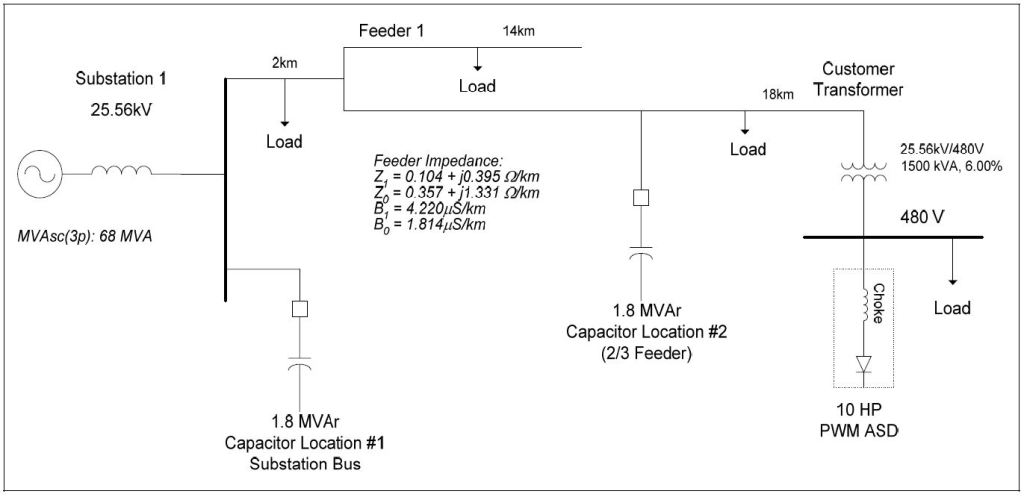
Transient overvoltages and nuisance tripping of a customer’s adjustable-speed drive during utility capacitor bank switching was studied for the system shown in Figure 1. The case involved determining overvoltage transients during uncontrolled capacitor bank switching as well as an evaluation of the effectiveness of synchronous closing control. The accuracy of the system model was verified using three-phase and single-line-to-ground fault currents and other steady-state quantities, such as capacitor bank rated current and voltage rise.
Figure 1 – Oneline Diagram for the Synchronous Closing Evaluation Case Study
A typical 10 hp customer adjustable-speed drive was included in the simulation model to determine the potential for nuisance tripping of the drive when a 1.8 MVAr, 25.56kV capacitor bank is switched at either the substation bus or at a location that is 2/3 of the feeder length. The energizing frequency for the 1.8 MVAr, 25.56kV distribution capacitor bank with a source strength of 68 MVA may be approximated using the following expression:
.
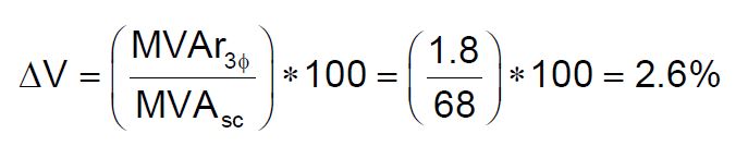
The steady-state voltage rise for this case may be approximated using the following expression:
.
A maximum voltage rise design limit of 3% would mean that the largest capacitor bank that can be switched at the substation for the studied circuit would be approximately 2 MVAr. Installation of a larger substation capacitor bank, such as 6 MVAr, would result in an excessive steady-state voltage rise (8.8%) and would likely require a circuit reconfiguration.
SIMULATION RESULTS
The effectiveness of synchronous closing control on the capacitor bank switch was evaluated in a series of cases that varied the timing error from an ideal voltage zero closing. Synchronous closing is independent contact closing of each phase near a voltage zero. Previous analysis has indicated that a closing consistency of ±1.0msec provides overvoltage control comparable to properly rated pre-insertion resistors. The success of a synchronous closing scheme is often determined by the ability to repeat the process under various (system and climate) conditions.
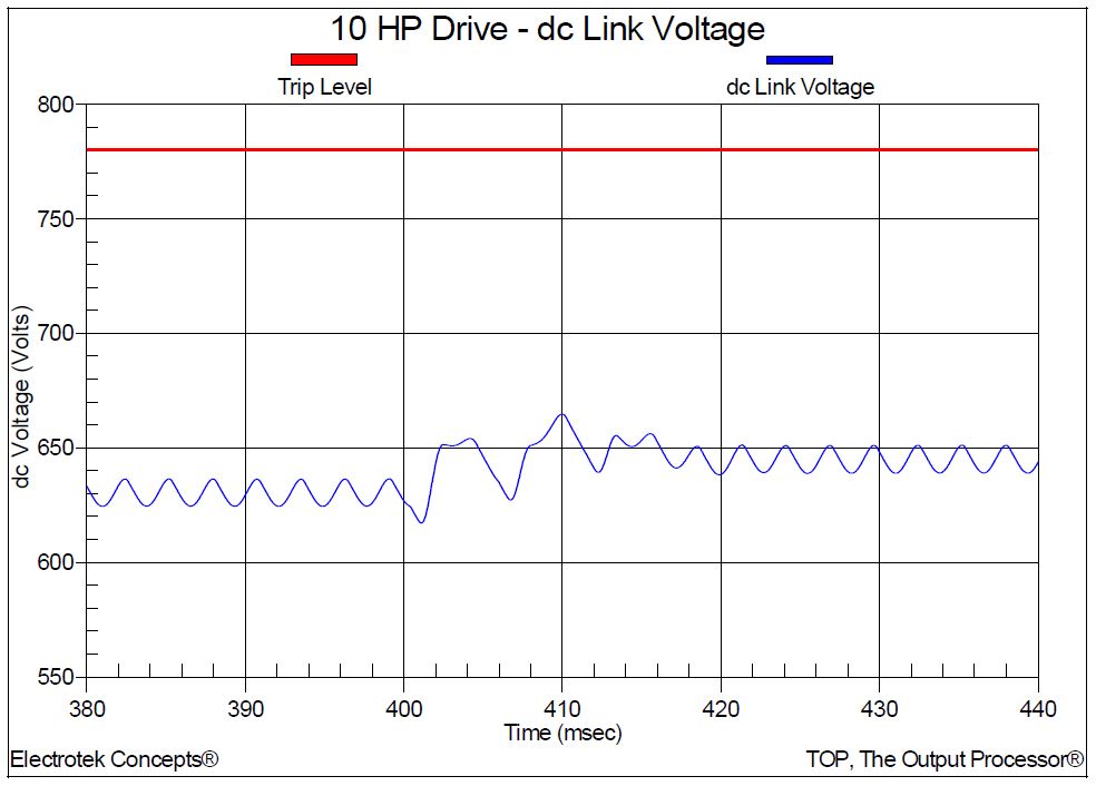
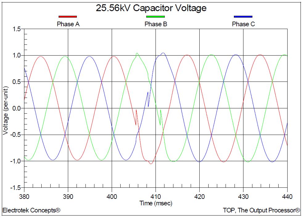
Simulation results are summarized in Table 1. The maximum transient overvoltage (refer to Figure 2) at the 25.56kV bus when energizing the 1.8 MVAr capacitor bank at the substation bus was 1.26 per-unit. Typical overvoltage magnitude levels range from 1.1 to 1.5 per-unit for smaller substation and feeder capacitor banks. The maximum transient overvoltage (refer to Figure 3) at the customer’s 480V bus was 1.09 per-unit. The resulting dc voltage on the 10 hp adjustable-speed drive in the customer facility was 665 volts (refer to Figure 4) which is lower than the assumed trip level of 780 volts, so it is assumed that the drive will not trip for this case.
Table 1 – Summary of Simulation Results for Synchronous Closing Evaluation
.
Figure 2 – Substation Bus Voltage during Capacitor Bank Energization
Figure 3 – Customer’s 480 Volt Bus Voltage during Capacitor Bank Energization
Figure 4 – ASD dc Link Voltage during Capacitor Bank Energization
Figure 5 shows the resulting 25.56kV bus voltage for the worst-case synchronous closing control case with a +1.0msec error. The maximum transient overvoltage is reduced from 1.26 per-unit to 1.03 per-unit. The customer’s 480 volt bus voltage is reduced from 1.09 per-unit to 1.01 per-unit and the dc voltage on the 10 hp adjustable-speed drive is reduced from 665 volts to 632 volts. The maximum transient overvoltage (refer to Figure 6) at the 25.56kV feeder location when energizing the 1.8 MVAr capacitor bank at 2/3 of the feeder length was 1.32 per-unit. The maximum transient overvoltage at the customer’s 480V bus was 1.18 per-unit. The resulting dc voltage on the 10 hp adjustable-speed drive in the customer facility was 699 volts, which is lower than the assumed trip level of 780 volts, so it is assumed that the drive will not trip for this case.
Figure 5 – Substation Bus Voltage with Synchronous Closing Control
Figure 6 – Feeder Voltage during Capacitor Bank Energization
Figure 7 shows the resulting 25.56kV feeder voltage for the worst-case synchronous closing control case with a +1.0msec error. The maximum transient overvoltage is reduced from 1.32 per-unit to 1.05 per-unit. The customer’s 480 volt bus voltage is reduced from 1.18 per-unit to 1.03 per-unit and the dc voltage on the 10 hp adjustable-speed drive is reduced from 699 volts to 661 volts.
Figure 7 – Feeder Voltage with Synchronous Closing Control
SUMMARY
Observations and conclusions for this case study include:
1.The devices and equipment being applied on the power system are more sensitive to power quality variations than equipment applied in the past. New equipment includes microprocessor-based controls and power-electronic devices that are sensitive to many types of disturbances. Controls can be affected, resulting in nuisance tripping or misoperation as part of an important process, or actual device failure can occur.
2.Capacitor bank switch selection and configuration will generally depend on switch capabilities (e.g., short circuit interrupting and capacitance switching ratings), mitigation device selection (e.g., pre-insertion vs. synchronous closing), site considerations, and an economic evaluation.
3.Transient overvoltages at the substation bus and feeder capacitor bank location when energizing the 1.8 MVAr capacitor bank were 1.26 per-unit and 1.32 per-unit respectively. These values are well below arrester protective levels for the simulated system and the simulated adjustable-speed drive did not trip for both cases without and with synchronous closing control.
4.Transient overvoltages associated with energization of the 25.56kV capacitor bank can be reduced with the application of synchronous closing control. The resulting overvoltages at the substation bus and feeder capacitor bank location were 1.03 per-unit and 1.05 per-unit respectively. In addition, the resulting overvoltages at customer’s 480 volt bus were also reduced, thereby significantly reducing the probability of localized customer problems due to sensitive equipment or low voltage power factor correction.
5.For the studied system, it is unlikely that the energization of a 1.8 MVAr capacitor bank at either the substation bus or feeder location will create transient overvoltages severe enough to cause problems for customer systems.
REFERENCES
G. Hensley, T. Singh, M. Samotyj, M. McGranaghan, and T. Grebe, Impact of Utility Switched Capacitors on Customer Systems Part II – Adjustable Speed Drive Concerns, IEEE Transactions PWRD, pp. 1623-1628, October, 1991.
G. Hensley, T. Singh, M. Samotyj, M. McGranaghan, and R. Zavadil, Impact of Utility Switched Capacitors on Customer Systems – Magnification at Low Voltage Capacitors, IEEE Transactions PWRD, pp. 862-868, April, 1992.
Electrotek Concepts, Inc., Evaluation of Distribution Capacitor Switching Concerns, Final Report, EPRI TR-107332, October 1997.
RELATED STANDARDS IEEE Std. 1036-1992
GLOSSARY AND ACRONYMS ASD: Adjustable-Speed Drive PWM: Pulse Width Modulation MOV: Metal Oxide Varistor TVSS: Transient Voltage Surge Suppress
Published by Petr KREJCI1, Pavel SANTARIUS1, Radovan HAJOVSKY1, Richard VELICKA1, Radim CUMPELIK2 VSB – Technical University of Ostrava, Czech Republic (1), CEZ, a.s., Czech Republic (2)
Abstract. In the paper, the results of the complex monitoring of selected PQ parameters during 12 years will be summarized together with the comparison of the changes of parameters after three years on all voltage levels (HV, MV and LV) in the power company CEZ in the North Moravia Region. In addition the results of annual continual monitoring for one selected locality on MV level will be presented in the paper.
Streszczenie. W artykule przedstawiono wyniki kompleksowej, trwającej 12 lat, obserwacji wybranych parametrów jakości energii elektrycznej oraz porównanie zmian podstawowych parametrów po 3 latach w sieciach o różnych poziomach napięć (WN, SN i nn) w przedsiębiorstwie energetycznym CEZ w rejonie Północnych Moraw (Monitorowane jakości energii w wybranych sieciach w Republice Czeskiej).
Keywords: Power quality, harmonics, flicker, unbalance. Słowa kluczowe: Jakość energii, harmoniczne, fluktuacja napięcia, asymetria.
Introduction
The electrical power quality is assessed by the CSN EN 50 160 standard via 13 parameters of voltage. Extensive use of appliances with non-linear characteristics in LV distribution networks (appliances such as TVs, computers, copy machines, compact lights, etc.) is substantially deteriorating to quality parameters of electrical energy supplied.
In the former regional power company SME, a.s. (currently member of the CEZ group) in the Czech republic, there was, in 1997, a complex monitoring of selected parameters of voltage quality initiated for distribution networks of this company. Step by step, individual supply nods 110 kV for all 6 supply areas of the company were measured. The whole cycle is rendered in 3-year cycles, so, as of 2010, the fifth measurement cycle is being rendered (with 1 year time-out in 2009). So, that is how, step by step, information on changes in periods of three years is being measured.
The method of power quality evaluation
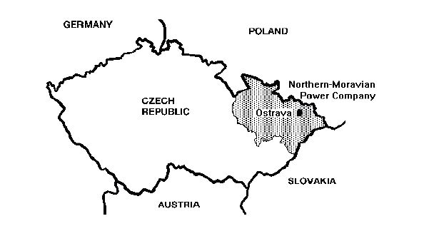
In the power company CEZ (in the North Moravia Fig. 1) the monitoring of a number of selected parameters of the quality of electrical energy (harmonics, flicker, unbalance) is being done in cooperation with research laboratories of the Department of Measurement and Control and Department of Electrical Power Engineering, Faculty of Electrical Engineering and Computer Science, VSB – Technical University of Ostrava.
Fig. 1. The North Moravia Region, the Czech Republic
Monitoring of the power quality was gradually done in individual parts of the company. The measuring was done in a complex way within the HV, MV and LV distribution. The program of complex quality of electrical energy evaluation was done in 59 LV distribution transformer station. The composition of consumption in the LV network was similar in all measured localizations – i.e. a mix of family houses and blocks of flats and small services.
In accordance with the Standard CSN EN 50 160, the measuring and evaluation of the power quality of single points was done in one week intervals, while the parameters of quality were evaluated for 10 minute intervals in the course of measuring. The measurement is separated to 6 stages. As individual parts of the company have 8-10 feeding nodes 110 kV, the monitoring was organized in half-year cycles, thus the whole program lasted for 3 years.
In single feeder points they evaluate measured data in all phases and on all voltage levels:
Selected voltage harmonics (3., 5., 7., 9., 11.)
Flicker
Unbalance
The trends of changes of the selected parameters
As it was stated, the monitoring of the quality parameters was started in 1997 in all feeding points and was done during three years. In 2002 the second cycle of monitoring was completed in the same sites, therefore it is possible to evaluate the trends of change during three years. In 2005 the third cycle and in 2008 the fourth cycle of monitoring was completed and in 2010 the fifth cycle of monitoring was started after 1 year time-out in 2009.
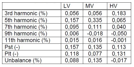
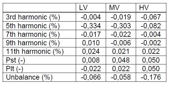
In the Table 1 the changes of the selected quality parameters are summarized (selected harmonics, flicker and unbalance) during the first 3 years in the LV, MV and HV network. In the Table 2 and Table 3 the changes of the selected quality parameters are summarized during the second and the last 3 years. Ref. [1]
Table 1. Trends of changes of the selected quality parameters between 1st and 2nd cycle(in years 1997-2002)
.
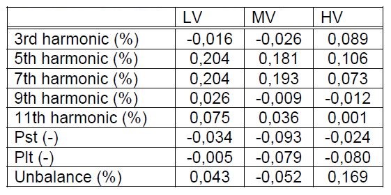
Table 2. Trends of changes of the selected quality parameters between 2nd and 3rd cycle (in years 2000-2005)
.
Table 3. Trends of changes of the selected quality parameters between 3rd and 4th cycle (in years 2003-2008)
.
Evaluation of the trends of development of the selected quality parameters
As for harmonics, the results are relatively positive, the values of individual harmonic components are significantly below the values of compatible levels, changes after 3 years are minimal. As for unbalance, the changes are also quite small.
As for flicker, in years 1997-2002 the situation was worse, the increase of Pst and Plt parameters was relatively low in relation to the level 1,0 (10-16%), but in relation to the real values the increase was significantly higher (around 40%). But in years 2000 – 2005 there was stabilization or even decrease of flicker parameters.
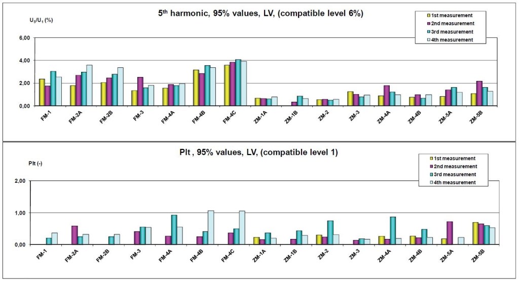
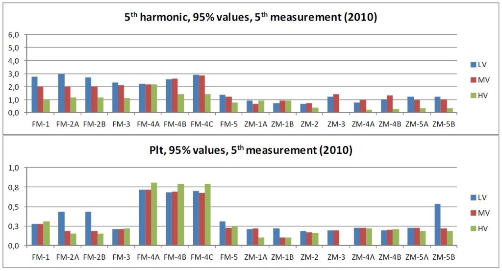
The fourth cycle of measurement indicates rather stagnation of quality parameters. On the Figure 2 and on the Figure 3 there are shown 95% values of 5th harmonic and flicker of 4 cycles of measurements in the LV distribution and values of 5th harmonic and flicker in LV, MV and HV networks in the fifth cycle of monitoring. Ref. [2]
Fig.2. 5th harmonic and flicker (Plt) in some LV networks
Fig.3. 5th harmonic and flicker (Plt) in some LV, MV and HV networks in the fifth cycle of monitoring
Quality parameters monitoring at all times
As of 2001, there are analyzers QWave (manufactured by LEM) fitted to distribution points of 110 kV so as it is possible to register as much information on individual parameters of voltage quality and events in the distribution system, as possible. QWave Power measures, simultaneously, all voltage quality parameters and compares it with the limit values according to the CSN EN50160 standard, and furthermore, it also renders the current analysis. QWave Light is a simplified version, evaluating only current for its all guaranteed and indicative parameters.
The rules for operation of distribution networks (DN) contain Annex 3 (Quality of electrical power in the distribution system, manners of determination and evaluation). Based on these rules, there must be quality analyzer of the electrical power supply fitted at all times, as of January 1, 2006, for all HV supply terminals, and as of January 1, 2007, for all supplies from DN 110 kV. The data acquired by these analyzers are being continuously processed and archived. Ref. [2]
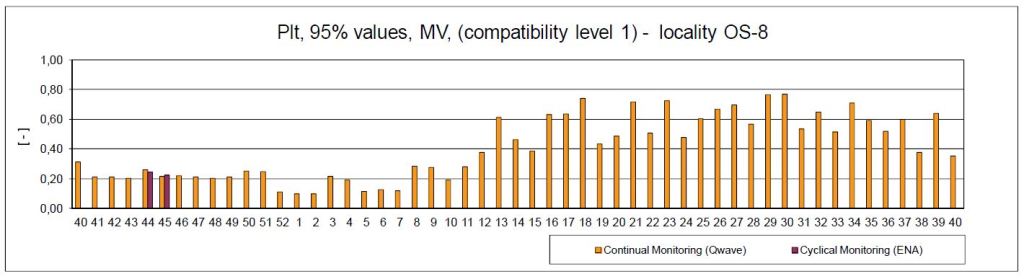
On the Figure 4 you can see the illustration of the continuously monitoring power quality parameters at the selected place OS-8 MV distribution network. On the diagram there are also placed the results acquired by the cyclic monitoring at the same place as it was described in the previous part of the contribution. For example, you can see that the values of flicker acquired by the cyclic monitoring makes approximately one quarter of the maximal value acquired by the yearly monitoring.
Fig.4. Flicker (Plt) in MV network OS-8
Use of intelligent electrometers for monitoring of quality parameters
Characteristic parameters of voltage within low and high voltage networks are introduced in the standard ČSN EN 50160. The revised normative ČSN EN 50160 further defines parameters for very-high voltage networks.
Current intelligent electrometers usually provide data that is not in compliance with the normative mentioned above, but they afford relevant data for energy companies usable in operation.
As for usage in operation of distribution, the most crucial issues are long-term monitoring of voltage deviations and their evaluation in compliance with standard ČSN EN 50160. Further important values are overvoltage, falls and short-time blackouts typically with 1s sample period (thus quite not in accordance with ČSN EN 50160). Yet this data can give a power company relevant information, because events longer than 1 second still report about the conditions of distribution network and during the changes (usually rising) they indicate the error states. Unfortunately, these data are recorded as events, but the number or logged events are limited and set low.
Harmonics and THD, even evaluated until low frequencies only (till 10th or 25th harmonic multiple), can provide relevant information. For example, when the third harmonic element rises, it can indicate the problem of power transformer. A significant rise of any harmonic or THD indicates the problem with resonances in distribution network.
Conclusions
In the paper above there are summarized the results of a long-term monitoring of the selected power quality parameters of the distribution networks together with the evaluation of the trends of change in the three years periods and results of continual monitoring PQ in selected MV distribution network.
The biggest changes were registered for flicker, in years 1997-2002 the situation was worse, the increase of Pst and Plt parameters was relatively low in relation to the level 1,0 (10-16%), but in relation to the real values the increase was significantly higher (around 40%). But in years 2000 – 2005 there was stabilization or even decrease of flicker parameters.
The results from continuously monitoring of power quality parameters manifest that the measured values can differ during the year and therefore the continuously monitoring is well-founded.
Current intelligent electrometers usually provide data that is not in compliance with the normative mentioned above, but they afford relevant data for energy companies usable in operation.
Acknowledgment
This contribution was supported by the Czech Science Foundation (No. GA ČR 102/09/1842).
REFERENCES
[1] Santarius P., Krejci P., Spacil D., Vasenka P. Power Quality Problems in Regional Distribution Networks in the Czech Republic. Conference “EPQU 2007”, Barcelona, Spain [2] Santarius P., Krejci P., Chmelikova Z., Ciganek J. Long-term Monitoring of Power Quality Parameters in Regional Distribution Networks in the Czech Republic. Conference “ICHQP 2008”, Wollongong, Australia
Authors: Doc. Ing. Petr Krejci, Ph.D., petr.krejci@vsb.cz Prof. Ing. Pavel Santarius, CSc., pavel.santarius@vsb.cz Ing. Radovan Hajovsky, Ph.D., radovan.hajovsky@vsb.cz Ing. Richard Velicka, Ph.D., richard.velicka@vsb.cz Ing. Radim Cumpelik, radim.cumpelik@cez.cz VSB – Technical University of Ostrava 17.listopadu 15, 708 33 Ostrava – Poruba, Czech Republic
Source & Publisher Item Identifier: PRZEGLĄD ELEKTROTECHNICZNY (Electrical Review), ISSN 0033-2097, R. 88 NR 7b/2012
Published by Electrotek Concepts, Inc., PQSoft Case Study: Distribution System Transient Measurement Data Evaluation, Document ID: PQS1012, Date: October 15, 2010.
Abstract: This case study presents a utility distribution system transient measurement data analysis. The distribution system included a number of feeders that supplied a mix of residential, commercial, and industrial customers. The causes of the transients measured during the monitoring period included capacitor bank switching, transformer energizing, single-phase faults, recloser operations, switch failures, and current-limiting fuse operations.
INTRODUCTION
A utility distribution system transient measurement data analysis case study was completed for the system shown in Figure 1. The 12.47 kV utility substation included a 30 MVA, 69 kV/12.47 kV step-down transformer and a number of distribution feeders that supplied a mix of residential, commercial, and industrial customers. There was a 6,000 kVAr, 12.5 kV capacitor bank at the substation bus that was energized using a synchronous closing control switch. In addition, each of the distribution feeders had a number of fixed or switched capacitor banks being used for power factor correction and voltage control.
The monitoring period was for one year and utilized power quality instruments that sampled voltages at 256 points-per-cycle and currents at 128 point-per-cycle. The sampling rate allowed characterization of low-to-medium frequency oscillatory transients. The measurement analysis was completed using the PQView® program. The causes of the transients measured during the monitoring period included capacitor bank switching, transformer energizing, single-phase faults, switch failure, recloser operations, and current-limiting fuse operations.
Figure 1 – Illustration of Oneline Diagram for Transient Measurement Data Evaluation
MEASUREMENT RESULTS
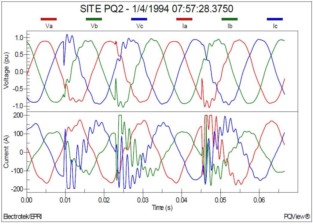
Figure 2 shows the measured voltage (per-unit) and current (A) waveforms during uncontrolled energization of the pole-mounted 600 kVAr capacitor bank on feeder #1. The measurement site was PQ2. The capacitor bank was switched on-and-off each day using time clock controls in an attempt to maintain a relatively constant voltage profile. The peak magnitude of the measured transient voltage was 1.09 per-unit and the principal frequency for the capacitor energizing waveform was approximately 650 Hz. The capacitor bank was energized using three single-phase mechanical oil switches with a pole span of approximately 3-5 cycles.
Typical voltage magnitude levels for switching distribution capacitor banks range from 1.3 to 1.5 per-unit and typical transient frequencies generally fall in the range from 300 to 1000 Hz. Power quality problems related to utility capacitor bank switching include customer equipment damage or failure, nuisance tripping of adjustable-speed drives or other process equipment, transient voltage surge suppressor failure, and computer network problems.
Figure 2 – Illustration of Feeder Capacitor Bank Energizing
Figure 3 shows the measured current waveform during back-to-back capacitor bank switching on feeder 2. Energizing a shunt capacitor bank with an adjacent capacitor bank already in service is known as back-to-back switching. High magnitude and frequency currents will flow between the capacitor banks when the second capacitor bank is energized. The measurement site was PQ3. The waveform shows the current that flows between the two 1,800 kVAr capacitor banks when the second capacitor bank is energized with the first capacitor bank already in service. The magnitude of the peak current was 600 A and the principal frequency was about 2.0 kHz.
The high-frequency inrush current may exceed the transient frequency momentary capability of the switching device (e.g., ANSI Std. C37.06-2000) as well as the I2t withstand of the capacitor fuses. It may also cause false operation of protective relays and excessive voltages for current transformers (CTs) in the neutral or phase of grounded-wye capacitor banks.
Figure 3 – Illustration of Back-to-Back Capacitor Bank Energizing
Figure 4 shows the measured 12.47 kV distribution feeder current waveform before-and-after energization of the pole-mounted 900 kVAr capacitor bank on feeder #3. The capacitor bank was switched on-and-off each day at the same time using a time clock control. The measurement site was PQ4.
The peak transient current for the capacitor bank energization portion of the event was 460 A. Insertion of the 900 kVAr capacitor bank creates a harmonic resonance that results in higher levels of current distortion. The steady-state total harmonic current distortion (ITHD) after energization of the capacitor bank was 13.26%.
Utilities switch capacitor banks in-and-out of service routinely to provide voltage support and to improve power factor. One potential disadvantage of capacitor bank switching is the effect that such an operation can have on the topology of the system. Switching capacitor banks into mostly inductive circuits can tune the natural frequency of the circuit closer to harmonic frequencies that might be prevalent on the system. Obviously, this can be a significant problem, possibly resulting in severe voltage and current distortion, increased losses, and overheating of system equipment.
Figure 4 – Illustration of Capacitor Bank Energizing and Harmonic Resonance
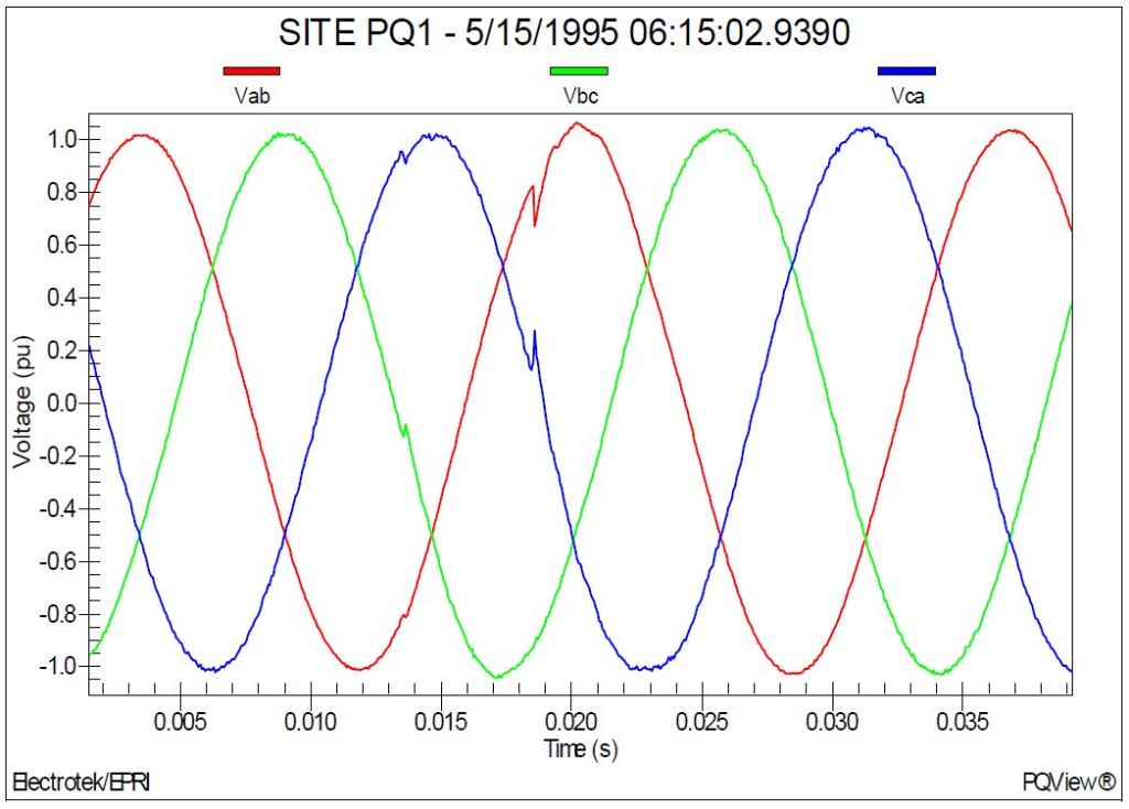
Figure 5 shows the measured voltage (per-unit) waveforms during energization of the substation 6,000 kVAr capacitor bank on feeder #1. The capacitor bank was switched using synchronous closing control. The measurement site was PQ1. The magnitude of the transient voltage at the substation bus was 1.06 per-unit.
Synchronous closing is independent contact closing of each phase near a voltage zero. To accomplish closing at or near a voltage zero (avoiding high prestrike voltages); it is necessary to apply a switching device that maintains a dielectric strength sufficient to withstand system voltages until its contacts touch. Although this level of precision is difficult to achieve, closing consistency of ±0.5 milliseconds should be possible. Previous research has indicated that a closing consistency of ±1.0 millisecond provides overvoltage control comparable to properly rated pre-insertion resistors. The typical transient overvoltage range for synchronous closing control would be between 1.05 and 1.20 per-unit depending on the capacitor bank rating and a number of other system parameters.
The success of a synchronous closing scheme is often determined by the ability to repeat the process under various (e.g., system and climate) conditions. Adaptive, microprocessor-based control schemes that have the ability to learn from previous events address this concern. The primary benefits of this capability are the control’s ability to compensate for environmental factors and the increased reliability (less maintenance) that can be achieved. Grounded capacitor banks are controlled by closing the three phases at three successive phase-to-ground voltage zeros (60° separation). Ungrounded banks are controlled by closing the first two phases at a phase-to-phase voltage zero and then delaying the third phase 90 degrees (phase-to-ground voltage zero).
Figure 5 – Illustration of Capacitor Bank Energizing with Synchronous Closing
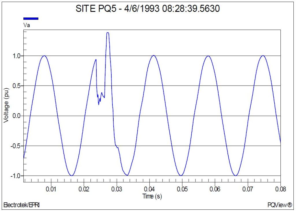
Figure 6 shows the measured voltage (per-unit) and current (A) waveforms during a ferroresonance event on feeder #4. The measurement site was PQ5. The magnitude of the ferroresonant voltage at the monitoring location was 1.42 per-unit. The cause of the ferroresonance event was an unbalanced operation caused by a single-phase fuse operation on a customer step-down transformer.
Ferroresonance is a term generally applied to a wide variety of interactions between capacitors and iron-core inductors that result in unusual voltages and/or currents. In linear circuits, resonance occurs when the capacitive reactance equals the inductive reactance at the frequency at which the circuit is excited. Iron-core inductors have a nonlinear characteristic and therefore a range of inductance values. This relationship may lead to a number of operating conditions where the inductive reactance does not equal the capacitive reactance, but very high and damaging overvoltages occur.
If high voltages accompany the ferroresonance, there could be electrical damage to both the primary and secondary circuits. Surge arresters commonly fail during this condition. Arrester failures are related to the heating of the arrester block, and at times, the failures can be catastrophic, with parts being expelled from the arrester housing. In a typical power system, ferroresonance occurs when a transformer becomes isolated on a cable section in such a manner that the cable capacitance appears to be in series with the magnetizing characteristic of the transformer. An unbalanced switching operation is required to initiate the condition. Ferroresonance cannot always be entirely avoided. However, steps can be taken to reduce the probability of occurrence.
Figure 6 – Illustration of Distribution Feeder Ferroresonance
Figure 7 shows the measured current (A) waveform during a transformer energizing event on feeder #4. The measurement site was PQ5. The peak magnitude of the primary inrush current at the monitoring location was 46 A and the duration of the event was approximately 10 cycles. The cause of the transformer inrush was a recloser operation during circuit restoration.
Energizing saturable devices (devices with magnetic cores), such as power transformers, results in inrush currents that are rich in harmonic components. The inrush current interacts with the system impedance vs. frequency characteristics to create a voltage waveform that can have significant harmonic components for the duration that the inrush current is present. Transformer inrush current typically decays over a period on the order of one second.
This phenomenon combines concerns for harmonic current distortion and transient voltages. The harmonics of concern are low order (dominated by the 2nd through the 5th harmonics). If the circuit has a high impedance resonance near one of these frequencies, a dynamic overvoltage condition results that can cause failure of arresters and problems with sensitive equipment.
This problem is typically limited to cases of energizing large transformers with large power factor correction capacitor banks (e.g., arc furnace installations or other large industrial facilities). The solution to problems with dynamic overvoltages is to make sure that the conditions causing the system resonance are not present when the transformer is energized. This could mean making sure a capacitor bank is out of service whenever a large transformer is energized.
Figure 7 – Illustration of Transformer Inrush during Circuit Restoration
Figure 8 shows the measured voltage (per-unit) waveform during the operation of a current-limiting fuse (type 25K CL) on feeder #4. The measurement site was PQ5. The maximum peak arc voltage for the event was approximately 140% (1.40 per-unit). The fault was cleared by the fuse in approximately ½ cycle.
Current-limiting fuses are often used in electrical equipment where the fault current is very high and an internal fault could result in a catastrophic failure. There are various designs, but the basic configuration is that of a thin ribbon element or wire wound around a form and encased in a sealed insulating tube filled with a special sand. The tube is constructed of stout material such as a fiberglass-epoxy resin composite to withstand the pressures during the interruption process without rupturing. The element melts in many places simultaneously and, with the aid of the melting sand, very quickly builds up a voltage drop that opposes the flow of current. The current is forced to zero in about ¼ cycle.
The main purpose of current-limiting fuse is to prevent damage due to excessive fault current. They have the beneficial side effect with respect to power quality that the voltage sag resulting from the fault is very brief. The voltage sag is so short that not many industrial processes will be adversely affected. Therefore, one proposed practice is to install current-limiting fuses on each lateral branch in the high fault current region near the substation to reduce the number of sags that affect industrial processes.
Figure 8 – Illustration of a Current Limiting Fuse Operation
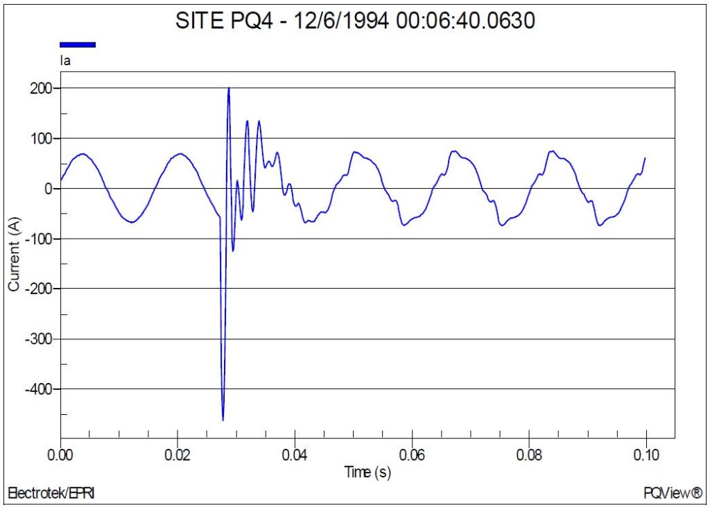
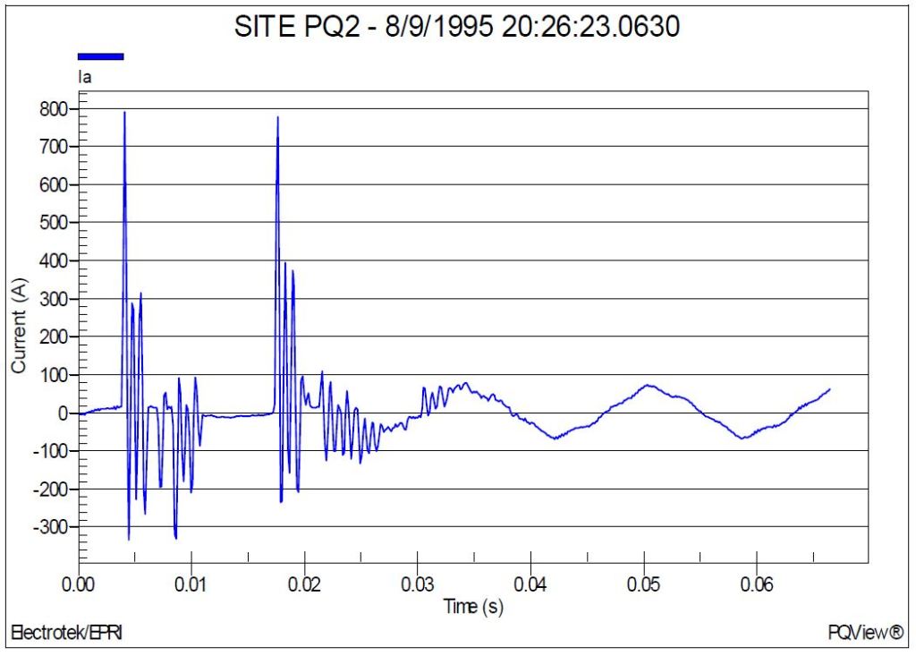
Figure 9 shows the measured current (A) waveform during an arcing fault on feeder #1. The measurement site was PQ4. The fault occurred during a thunderstorm and it was cleared in approximately 4 cycles by a recloser on an adjacent feeder.
Arcing faults are quite common on distribution and transmission feeders. These types of faults are usually caused by lightning strikes to the circuit, tree limbs contacting the circuit, or animals contacting the circuit. Arcing faults often contain a significant third harmonic component. Consequently, the arcing voltage waveform often has a “flat-top” appearance, resembling a square-wave. The arcing current typically exhibits a continuous ringing. This characteristic can be attributed to the ringing between the system inductance and capacitance as the voltage changes suddenly as occurs with the step change of a square-wave.
With respect to arcing faults, thunderstorms subject distribution systems to double jeopardy. Not only does the lightning associated with the storm create the potential for flashovers, but the wind associated with the storm increases the chance of tree limb contact. An example of an arcing fault voltage is shown in Figure 10, which shows a measured voltage waveform during an arcing fault on a feeder #3. The fault occurred during a storm that was caused by a tree limb being blown into one phase of the distribution line.
Figure 9 – Illustration of a Current Waveform during an Arcing Fault Event
Figure 10 – Illustration of a Voltage Waveform during an Arcing Fault Event
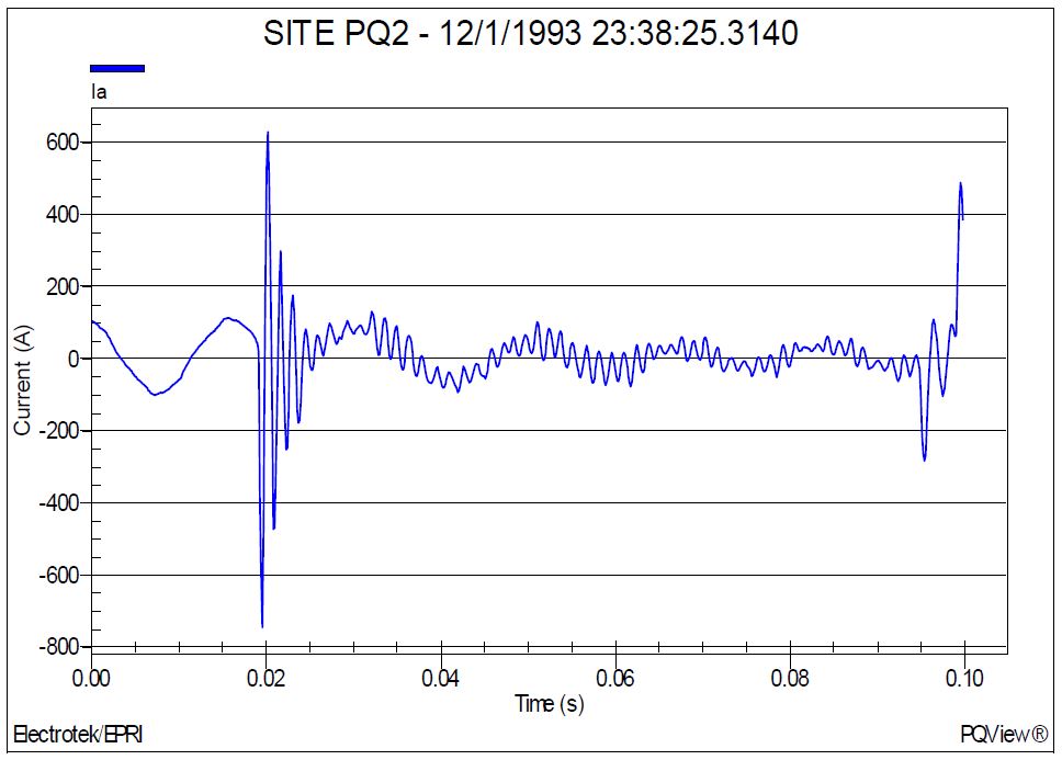
Figure 11 shows the measured current (A) waveform during a capacitor switch failure on feeder #1. The measurement site was PQ2. The maximum transient current magnitude for the event was approximately 790 A. Many similar transient waveforms were recorded at the monitoring site during a one-week period. These events showed that the switch performance had continue to deteriorate.
As the capacitor switch began to fail, abnormal events including arcing and pre-striking occurred. These were the initial warning sign that a more serious failure was about to occur. Closer examination of the waveform indicated that the pole of the switch did not properly close, possibly bouncing. This abnormal event resulted in two distinct energizations. First, the pole bounces, making a connection temporarily, but it does not latch. This results in an arc that extinguishes as the contacts pull apart. As the switch continues to close, however, the pole finally latches, and the capacitor bank was energized.
Figure 11 – Illustration of a Current Waveform during a Capacitor Bank Switch Failure
SUMMARY
This case study summarized a distribution system transient measurement data analysis. The causes of the transients measured during the monitoring period included capacitor bank switching, transformer energizing, single-phase faults, recloser operations, switch failures, and current-limiting fuse operations.
REFERENCES
IEEE Recommended Practice for Monitoring Electric Power Quality,” IEEE Std. 1159-1995, IEEE, October 1995, ISBN: 1-55937-549-3.
R.C. Dugan, M.F. McGranaghan, S. Santoso, H.W. Beaty, “Electrical Power Systems Quality,” McGraw-Hill Companies, Inc., November 2002, ISBN 0-07-138622-X.
Published by Mehmet Sait CENGİZ1 University of Yüzüncü Yıl (1)
Abstract. System that all stakeholders compound the activities (production, transmission, distribution, sale, consumption) to product and to consume quality, constant, reliable and economic electric energy is called Smart Grid (SG) in electric. SG, which its most important component smart meter (Smart Metering-SM), are advanced energy metering devices that give more information than traditional energy meters and that measure the consumption of electric energy. It includes integration techniques and various software applications depending on characteristics of SM electric network. In this study, by giving information about infrastructure of automatic meter, AMI installation levels and its integration to system are explained. An experiment proving the advantages that SM provides to system and consumer has been made and its results have been interpreted.
Streszczenie. Układy typu smart meter dają znacznie więcej informacji zużytej energii niż klasyczne liczniki. W artykule przedstawiono infrastrukturę i metody dołączenie do sieci. (Eksperyment dotyczący zastosowania I kosztu licznmika typu smart meter)
Keywords: smart grids, power grids, smart meters, distribution grids. Słowa kluczowe: smart grid, smart meter.
Introduction
SM solution to meet the needs of metering can be remotely set for electric distribution companies; it provides a clear and advanced metering infrastructure (AMI) [1]. AMI solution is an infrastructure that allows electricity distribution companies to display subscribers who sell energy and consume energy, to manage electricity consumptions, to measure the power quality, to increase reliability of distribution and that provides to meet completely the requests of operations, engineers, subscriber services and market regulatory supreme board in the field [2].
Even though automatic meter reading and its infrastructure (AMI) is one of the key works of Smart Network, SG is beyond the meter reading. Distribution Management, System Optimization and Energy Management System that has spread to the entire network should stand back of AMI so that electricity distribution system can efficiently support its own established system. AMI (Automatic Meter Infrastructure) solution allows electricity distribution company to realize a single SG application as modular and to make march forward and develop this system in time on its own request and then spread to entire network; or, by building a complete SG system, distributor company can begin to benefit from all of the advantages of smart network at once, without having any integration problem [3].
While AMI (Advanced Metering Infrastructure) is defined as transmission and management of energy over a network infrastructure in line with demand or in a regular way, bidirectional data exchange comes into question in advanced infrastructures [4]. In this way, not only transfer of data of energy consumption but also transmission of the other data that could be transmitted by center, such as cutoff and opening at the same time or reflecting the product selection to clients, is provided. SMs are the most important component of AMI. Installation of AMI should not be considered only as assembling or installation of meters. In advance of this, sufficient time and resource should be planned for planning, feasibility and design study of business processes [5]. In addition, throughout the entire process, institutional change and settlement should be managed in such a way as to meet the needs of distribution companies. In the projects to establish AMI, all of the following stages or a part of them, according to the needs of clients, should be made real [6].
AMI installation stages;
Planning of AMI infrastructure
Creation of Architecture
Revision of Business Processes
Creation of Functional Requirements
Evaluation of Suppliers and Solutions
Installation of Infrastructure and Making it Real
Distribution companies, primarily, should plan the factors related to infrastructure. Afterwards, beginning with installation of meters in the field, determination of functional and technical architecture consisting of communication infrastructure and central data acquisition systems and integration points should be done. After putting AMI systems into practice, it is required that to redesign the business processes that will change under distribution and retail sale operations and to demonstrate new business processes. To achieve the required results, it is important to redesign the business process by taking possible changes into account. In this direction, after analyzing current business processes and purposes, redesign should be performed. In next phases, installation of meters and dissemination studies should be practiced.
Concept And Effects Of Smart Grid
Through AMI, not only consumption information but also information about failure and cut-off are transmitted to centre. In this way, network operator can carry out wealth management (failure repair-maintenance system) in a more efficient way [9]. SM system that is a part of AMI consists of five main factors:
1.Home Network: Through the system that is also called Home Area Network (HAN), commands came from AMI provide to manage the other devices at home. For example; in a space where electricity price is cheaper, electric vehicle can be remotely charged (from work place, vacation, etc.) and home can be heated. More importantly, as a result of remote commands production based on solar and wind energy can be followed. In this way, unlicensed production can be practiced more efficiently. In timeframes when electric prices are favorable, energy can be stored through remote commands by HAN application.
2.Meter owner endpoints: SMs take part in connection points of production station, free consumers and the other consumers. In particular, practicing bidirectional data transmission in consumer side is one of the most important factors of smart network.
3.Network: Data obtained by meters are transmitted over communication infrastructures such as GSM/GPRS, BPL (Broadband Over Power Line) or PLC (Power Line Communication) and then reached to data base in centre of distribution network.
4.Data center: MDM (Meter Data Management) system, where the data transmitted from field are cleaned, incomplete data is completed and takes its final form by treated, is in here. Meter Data Management System (MDM) informs us about fault-maintenance management, customer services-invoicing, prediction-load follow-up, market management, distribution operations and investment planning.
5.Back office and management: All data obtained by smart meters are evaluated in the background and required decisions are made by achieving analytic reports. In this direction:
Distribution Network Management: Making decisions of new investment, fault repair-maintenance follow-up and planning,
Meter reading, opening and cut-off: Carrying out retail sale services in a cost-efficient, central and consistent way.
Invoicing and customer services: Remote invoicing, leak check or determination of decline at consumer consumption, checking the data of meter before invoice issue are practiced.
The most important acquisition of SG investments is reducing the cost and increasing the efficiency [10,11]. In the U.S.A and many European countries, SG and SM investments are preferred [12]. In our country, however, SG investments are called under the title of automatic meter reading system (OSOS) and becomes a current issue to transmission and distribution networks. OSOS is composed of remote reading of data automatically and data verification after transferring to a central system, completing the incomplete data and transmission to relative stakeholders in a proper format [13]. Through increased competition in the sale of energy, distribution companies that want to offer better service for their clients (product development, less cut-off), to reduce leaks and to move one step forward in wealth management should cross into SG investments without losing time.
Historically saving descriptive identity data related to SM, data of assessment and invoicing ( total active and reactive energy indices, periodical data of the highest demand, load profile curves ) and meter status information ( calibration time, low battery warning, opening warn of connector and case cover) in data centers will provide great advantages to have chances to report in different dimensions, to follow the measurement points timely and accurately and also to reduce loss leakage in large measure by feeding invoicing systems with consistent data [14,15]. Advantages are provided by SMs to system can be queued as :
• It provides steady and future guaranteed communication. It provides all of the required band width that will meet SG needs ( including the electric selling operation from hibrid automobiles to electricity distribution company) of AMI and sections.
• It provides inclusive network and operation management. To be able to display SG infrastructure provides a complete cycle management involving trouble shooting and maintenance management [16].
• Automatic data acquisition makes gain storage and analyzing ability. It manages meter data acquisition by providing standard interfaces to Meter Data Management of electricity distribution companies [16].
• It provides efficient communication solution in terms of cost. This solution communicate with many technologies including that broadband over power lines (BPL) by each Smart Transducer. Due to electricity distribution company communicate by using its own network with BPL technology, cost unit is lower [16].
Smart Meter Application Experiment
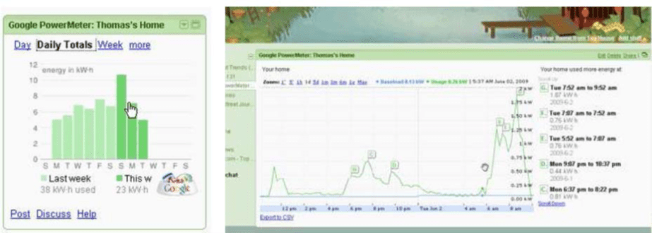
Remote meter reading systems that is one of the initial steps of SG system are found in many countries including Turkey. Many international companies that want to have a voice in future and/or infrastructure of these systems, installed web portals and act in common with electricity distributors. In this context Google, by PowerMeter system, offers an opportunity you to see your instant consumption and invoicing through a “Google Attachment” in a live presentation when you surf in the internet. Besides, savings of many consumers practiced by using this system has been indicated on website. Sample screen display indicating the detailed load graphic by Google Powermeter program is illustrated on Figure 1 [17,18].
Fig. 1. Google Powermeter attachment screen display and detailed load graphic
In the same way, Microsoft has also begun to provide service its users by Hohm. In the study made by system of Microsoft, system offers a survey about a home and devices in that home, after this an average consumption appears. Microsoft system has the possibility of recording manually invoices of consumers apart from remote reading system by SM. Distribution of load consumption of a sample home in Microsoft Hohm, is illustrated on Figure 2 [19].
Fig. 2. Screen display of Microsoft Hohm and distribution of a sample home consumption
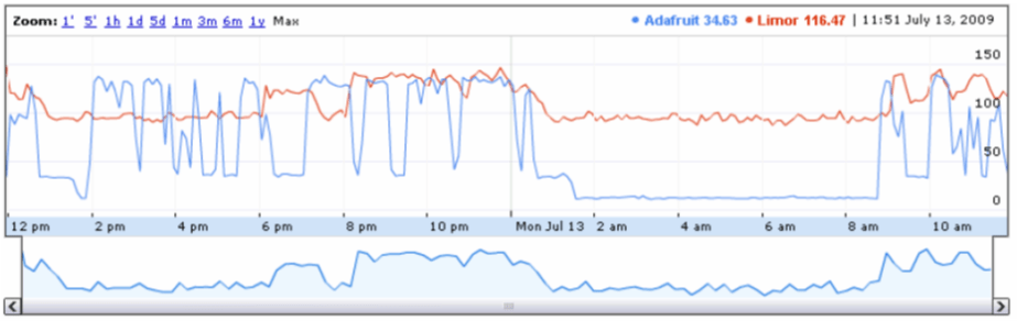
Fig. 3. Daily load usage from a site that uses Tweet-a-Watt
In the study that is made with reference to the idea that there will be a quite market for these systems in Turkey, through systems that could be found easily on internet, electricity consumption is read over wattmeter and then can be published on websites like Tweeter [20]. On “Tweet-a-watt” site that is one of the systems in question, consumption graphics are published with a system that costs 90 $ in average. Consumption graphic that shows daily load usage for any client, is illustrated on Figure 3 [21].
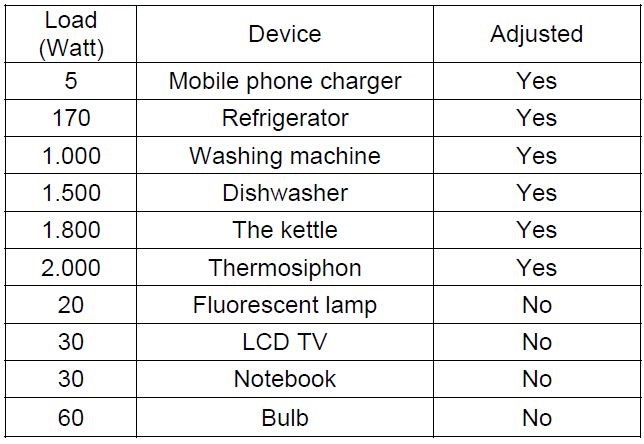
For this system, in Turkey, experimental status of such a system is obtained by wattmeter and electronically tuned sockets. While there is no “smart network” study in our country yet, there is a study about the advantages in case of a smart network and dimensions of demand side attendance. For this, by measuring the devices in a home through Wattmeter, instant load and hourly load values obtained. At this stage, in the experiment for demonstration purposes, data recorded transiently as if there is a remote reading system with smart meter. Information about instant loads, devices of the house, option of remote tuning are in Table 1.
Table 1. Instant loads, devices in the sample house and options of remote tuning.
.
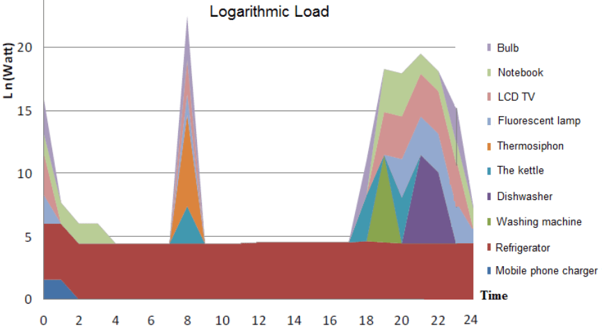
In here, while it depends on choice of consumer which tools will be turned off automatically, in a real system it is possible to control these sockets through electronic control devices can be installed into the sockets in the house. Average load consumption curve of a house in one day, has been obtained and is illustrated on Figure 4.
Fig. 4. Average load consumption curve of a house in one day
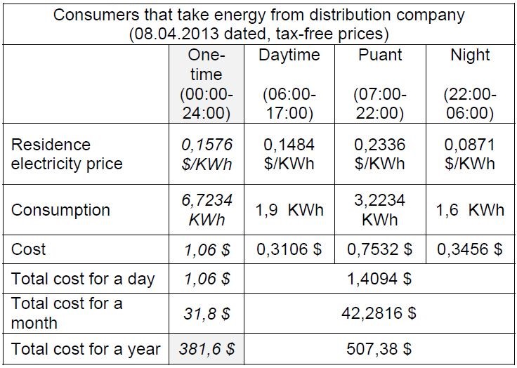
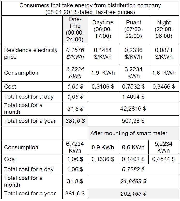
To see and demonstrate advantages of smart meters in consideration of these load consumptions, a comparison based upon one time and multi-time tariffs has been made. It is seen that using multi-time tariff over this system and consumption increases the cost to be paid. Due to client is at his home around 17:00 o’clock and maintains all the main activities until 24:00. A large part of hours when consumption is around the top level corresponds to the interval that energy price is the highest. Therefore, this client consumes the electricity in peak time, in other words, in the most expensive moments. To prevent this situation, smart meters can be used.
Table 3, for April of 2013, illustrating one-time and multi-time tariffs of public company TEDAŞ that is the biggest distribution company of our country, is in below. In table 2 also costs which occur on the basis of daily, monthly and annual as a result of being priced of the same consumption by one time and multi time tariff.
Table 2. 7 January 2013 dated electricity sale prices of TEDAŞ per tax-free KWh [22].
.
If loads that can be adjusted in consumption profile are transferred through programmable sockets to time zones in which consumption is more economic, in other words, in case of using SM, A severe load decline is provided by providing automatically to start dishwashers and washing machines up after 22:00. Besides, when electronic sockets are programmed in order to laptops would make battery consumption in puant consumption time and would charge in the end of puant, ultimate consumption, in a system that SMs check in, is like in Table 3.
Table 3. After shifting consumption times of devices can be tuned by SM.
.
The same amount of consumption before SM using, while monthly electric bill is 31,8 $ in one-time, annual consumption is 42,2816 $ in three-time consumption. In such a consumption, it is paid 32.95 % more. However, it becomes advantageous by including SMs in the system, is paid 21,8469 $ instead 31,8 $. Therefore, without making any limitation with the same consumption, it is paid 31.3 % less due to programming feature of smart meter. Consequently, while it is paid annual 381,6 $ in invoicing by one-time meter that is considered as the minimum cost, it is paid 262,1636 $ by multi-time meter in the system with smart meter. In other words, every consumer can economize 9.9544 $ per month and 119,4563 $ per year in total. SM usage has two-way advantage. These are economizing 9.9544 $ per month and moreover making network control easy by contributing to decline of puant load in the hours when power demand is huge in terms of network.
Conclusions
As a result of privatization of distribution companies, requirement of legal disintegration, increasing competition and technologic requirements , SM/SG necessity comes into prominence in distribution sector of Turkey. In this direction, distribution companies and the other stakeholders should be ready for change and transformation. SMs provide the following benefits to electricity distribution companies:
• Operational Cost Reduction: It allows to collect meter data of distribution companies and to reduce meter reading expenses based on work force. through this, distribution companies will have chance to reduce transport costs that occur against to subscriber telephones or fault reports by remote monitoring the subscriber interruptions.
• Revenue Protection: By providing real-time and clearer invoice details, it removes need of monthly invoice prediction. This model supports, on behalf of revenue protection, both prepayment systems and systems that cuts remotely electricity of subscribers who don’t pay their invoices. In conclusion, it supports application of “Energy Robbery Determination” to reduce deficiencies of distribution companies.
• Demand Management: It collects data from network and subscribers, one by one, for advanced level of pricing policies of electricity distribution companies such as pricing according to time when subscribers use electricity within day and/or pricing according to critical peak rates. In addition, it allows subscribers of distribution companies to see their own consumption amounts and to change their life styles in order to reduce or change load rates.
• Home Area Network – HAN: AMI solution provides remote control for distribution companies. By means of this, additional services such as remote opening-closing of meter, Internet connection service, security and automation of home, could be done.
As it can be seen through experiment that is carried out, SM usage has benefit in two way. These are reducing of price that will be paid monthly by consumer and moreover making network control easy by contributing to decline of puant load in the hours when power demand is huge in terms of network.
REFERENCES
[1] Har t DG. Using AMI to realize the smart grid. In: Proc. IEEE Power and Energy Society General Meeting – Conversion and Delivery of Electrical Energy. 2008. p. 1–2. [2] Chebbo M. EU smart grids framework: electricity networks of the future 2020 and beyond. In: Proc. IEEE Power Engineering Society General Meeting. 2007. p. 1–8. [3] Vojdani A. Smart integration. IEEE Power & Energy Magazine November 2008;6:71–9. [4] Lee PK, Lai LL. A practical approach of smart metering in remote monitoring of renewable energy applications. In: Proc. IEEE Power & Energy Society General Meeting. 2009. p. 1–4. [5] Mahmood A, Aami r M, Anis MI. Design and implementation of AMR smart grid system. In: Proc. IEEE Canada Electric Power Conference. 2008. p. 6–7. [6] Us Nist, 2013, Nist Framework And Roadmap for Smart Grid Interoperability Standards [online], http://www.nist.gov/smartgrid/upload/NIST_Framework_Release_2-0_corr.pdf [Ziyaret Tarihi: 3 Ocak 2012]. [7] Val igi E, Mar ino E. Networks optimization with advanced meter infrastructure and smart meters. In: Proc. International Conf. and Exhibition on Electricity Distribution. 2009. p.p.1–4. [8] Il-Kwon Y, Nam-Joon J, Young-Il K. Status of advanced metering infrastructure development in Korea. In: Proc. Transmission& Distribution Conference & Exposition: Asia and Pacific. 2009. p. 1–3. [9] Lee PK, Lai LL. Smart metering in micro-grid applications. In: Proc. IEEE Power & Energy Society General Meeting. 2009. p. 1–5. [10] Pacific Northwest GridWise Testbed Demonstration Projects, Part I. Olympic Peninsula Project, D.J. Hammerstrom et al., Ekim 2007, http://gridwise.pnl.gov/docs/opproject_final_rep.pdf [11] GridWise Demonstration Project Fast Facts, Pacific Northwest National Lab.,2007, http://gridwise.pnl.gov/docs/pnnl_.pdf [12] Tuan D. The energy web: concept and challenges to overcome to make large scale renewable and distributed energy resources a true reality. In: Proc. 7th IEEE International Conference on Industrial Informatics. 2009. p. 384–9. [13] Huc zala M, Lukl T, Misurec J . Capturing energy meter data over secured power line. In: Proc. International Conference on Communication Technology. 2006. p. 1–4. [14] Mai t ra S. Embedded energy meter – a new concept to measure the energy consumed by a consumer and to pay the bill. In: Proc. Joint International Conference on Power System Technology and IEEE Power India Conference. 2008. p. 1–8. [15] He MM, Reutzel EM, Xiaofan J, Katz RH, Sanders SR, Cul ler DE, et al . An architecture for local energy generation, distribution, and sharing. In: Proc IEEE Energy 2030 Conference. 2008. p. 1–6. [16] Cengiz M.S., Rustemli S., Almali M. N. The Advantages of the Applicability of New Generation Sectionalisers and Reclosers Over the Pole “Przeglad Elektrotechniczny” (Electrical Review), R. 89 NR 2a/2013, pp:155-159. 2013. [17] Google.org PowerMeter, http://www.google.org/powermeter [18] Images of Google PowerMeter, No Business Model, Katie Fehrenbacher, 2 Haziran 2009, http://earth2tech.com/2013/01/05/images-of-googlepowermter [19] Microsoft Hohm, 3 Ocak 2013, http://www.microsofthohm.com/Recommendations/ [20] Tweet-a-Watt kits now available, Adafruit Industries Blog, http://www.adafruit.com/blog/2013/01/02/tweet-awatt-kits-nowavailable [21] Tweet-a-Watt, http://wattcher.appspot.com/history?user=adawatt@gmail.com [22] TEDAS Elektrik satıs tarifeleri, http://www.tedas.gov.tr/tarifeler_xls/2013_trf/tarife.xls
Authors: Lecturer Mehmet Sait Cengiz, Department of Baskale Technical Vocational School, Yuzuncu Yil University, Van/Turkey, E-mail: msaitcengiz@gmail.com
Source & Publisher Item Identifier: PRZEGLĄD ELEKTROTECHNICZNY, ISSN 0033-2097, R. 89 NR 11/2013
Published by Electrotek Concepts, Inc., PQSoft Case Study: Distribution Feeder Wind Turbine Generator Analysis, Document ID: PQS1206, Date: January 26, 2012.
Abstract: This case study presents a distribution feeder wind turbine generator analysis. The investigation included several potential causes of turbine and feeder overcurrents and overvoltages, including wind speed variations, cut-out and cut-in switching operations, ground faults, and islanding during feeder isolation. Mitigation alternatives for high temporary overvoltages (TOV) on distribution feeders include application restrictions, grounding transformers, direct transfer trip schemes, and crowbar switches.
INTRODUCTION
A distribution feeder wind turbine generator analysis case study was completed for the system shown in Figure 1. The case study investigated several potential causes of turbine and feeder overcurrents and overvoltages, including wind speed variations, cut-out and cut-in switching operations, ground faults, and islanding during feeder isolation. The simulations were completed using the PSCAD® transient program. A transient model was created to simulate a relatively weak distribution feeder with a single wind turbine generator connected near the end of the feeder. The resulting voltages and currents during various switching and fault events were determined.
Figure 1 – Illustration of Oneline Diagram for a Distribution Feeder Turbine Analysis
SIMULATION ANALYSIS
The simulation model included a 12.47kV substation and distribution feeder supplying a 1.5 MW wind turbine generator connected near the end of the feeder. The model included a 600 kVAr capacitor bank connected at the substation bus and several additional 600 kVAr capacitor banks on the feeder. There was one distribution feeder included in the model.
The model was designed so turbine and feeder overcurrents and overvoltages during wind speed variations, turbine cut-out and cut-in switching operations, ground faults, and islanding during feeder isolation could be determined. The accuracy of the simulation model at 60 Hz was determined using simulated fault current magnitudes and other steady-state quantities, such as cable line charging (MVAr) and feeder load flow values (MW & MVAr). The representation of the system short-circuit equivalent at the 12.47kV source substation included:
Three-phase (I3φ) fault current: 4,000 A @ -85.0° (86 MVA) Single-line-to-ground (IφG) fault current: 3,000 A @ -85.0° (65 MVA)
These values were converted to ohms for the PSCAD representation, which included a three-phase voltage source with positive and zero sequence impedances and a 150 Ω damping resistor.
The 12.47kV distribution feeder and underground cable sections were modeled using the following impedance data:
Conductor: 4/0 AWG AL Length: 5,550 feet Positive sequence impedance (Z1): 0.1087 +j0.0653 Ω/1000’ Zero sequence impedance (Z0): 0.2567 +j0.0688 Ω/1000’ Line charging (B/2): 8.7 μmhos/1000’
It was assumed that positive and zero sequence line charging values were the same. The coupled π-section model was used to model each cable section. That assured accurate representation of both the series impedances, as well as the line charging of the underground feeder cable sections.
The turbine transformer was modeled using the three-phase, two-winding transformer model. The turbine step-up transformer data included:
Three Phase Rating: 2,000 kVA Secondary Voltage: 480 V (grounded-wye) Primary Voltage: 12.47 kV (grounded-wye) Nameplate Impedance: 5.75% (X/R Ratio = 10)
The 1.5 MW (1.67 MVA @ assumed 0.90 PF) wind turbine generator was modeled using a wound rotor induction machine model. The wound rotor induction machine can be used to represent an induction generator and it can be operated in either ‘speed control’ or ‘torque control’ modes. One 150 kVAr capacitor bank was connected to the 480 V secondary for reactive power support.
The wind turbine generator was controlled using PSCAD’s built-in wind turbine component. The inputs to the component include wind speed (Vw – m/s) and the mechanical speed of the machine connected to the turbine (W – rad/s). The pitch angle (Beta) of the turbine blades is entered in degrees if pitch control is enabled. If pitch control is disabled, the turbine is switched to stall control mode, where the turbine’s aerodynamic characteristics will determine the output torque. The component outputs include torque (Tm) and power (P), which are in per-unit based on the machine’s MVA rating.
The wind speed component models the wind speed available to the wind turbine generator. The input of the component is an external signal representing wind speed (ES – m/s) and the output is the wind speed available to the turbine (Vw – m/s). This component can be used to study a wind gust (or ramp) to determine the response of the control system. The wind turbine characteristics determine the input torque variations (torque control mode) supplied to the induction generator.
Case 1 included simulating a wind speed variation. The simulation time was 20 seconds and the timestep was 50μsec. The average wind speed was 15 m/s. The simulated wind speed is shown in Error! Reference source not found.. The figure shows the simulated wind speed between 5 and 20 seconds. The maximum speed gust was 27 m/s.
Figure 3 shows the corresponding turbine current (Phase A) for Case 1. The maximum value was 17.0 kA during the initial abrupt wind speed change between 8 and 9 seconds.
Figure 4 shows the simulated electromagnetic torque for Case 1, while Figure 5 shows the corresponding turbine power.
Figure 2 – Simulated Wind Speed for Case 1
Figure 3 – Simulated Turbine Current for Case 1
Figure 4 – Simulated Electromagnetic Torque for Case 1
Figure 5 – Simulated Turbine Power for Case 1
Case 2 included simulating cut-out and cut-in switching operations. The simulation time was 20 seconds and the average wind speed was 15 m/s. The sequence of events for the switching operation included opening (cut-out) the low voltage circuit breaker supplying the wind turbine generator at 10 seconds and closing (cut-in) the circuit breaker back in at 15 seconds.
Figure 6 shows the turbine current (Phase A) for Case 2. The peak current value was 78.2 kA when the circuit breaker opens. The oscillatory transient voltage is due to the interaction with the power factor correction capacitor.
Figure 7 shows the corresponding turbine voltage (Phase A) for Case 2. The peak voltage was 471 V (1.20 per-unit) when the circuit breaker opens.
Case 3 included simulating a ground fault at the low voltage wind turbine generator secondary bus. The simulation time was 20 seconds and the average wind speed was 15 m/s. The sequence of events for the ground fault included applying a single-phase-to-ground fault (Phase A) on the turbine generator bus. The fault did not clear during the simulation.
Figure 8 shows the turbine current (Phase A) for Case 3. The peak current value was 30.9 kA when the fault occurs.
Figure 9 shows the turbine voltage for Case 3. The fundamental frequency temporary overvoltage was 464 V (1.19 per-unit) during the single-phase fault. Figure 10 shows the corresponding 12.47kV feeder voltage. The temporary overvoltage was 12.014kV (1.18 per unit).
Figure 6 – Simulated Turbine Current for Case 2
Figure 7 – Simulated Turbine Voltage for Case 2
Figure 8 – Simulated Turbine Current for Case 3
Figure 9 – Simulated Turbine Voltage for Case 3
Figure 10 – Simulated Distribution Feeder Voltage for Case 3
Case 4 involved simulating an islanding condition by opening the circuit breaker on the 12.47kV primary side of the turbine transformer. The simulation time was 20 seconds and the average wind speed was 15m/s. The sequence of events for the islanding case included opening the circuit breaker at 10 seconds. There were no faults applied during the simulation.
Figure 11 shows the turbine current (Phase A) for Case 4. The peak current value was 32.5 kA when the circuit breaker opens. Figure 12 shows the corresponding simulated electromagnetic torque for Case 4.
Figure 11 – Simulated Turbine Current for Case 4
Figure 12 – Simulated Electromagnetic Torque for Case 4
SUMMARY
This case study presents a distribution feeder wind turbine generator analysis. The investigation included several potential causes of turbine and feeder overcurrents and overvoltages, including wind speed variations, cut-out and cut-in switching operations, ground faults, and islanding during feeder isolation.
Voltage regulation, islanding, and reverse power flow, and the resulting potentially severe temporary overvoltages, are three of the most important operating considerations for distributed generation applications having a single large wind turbine generator on a relatively weak distribution feeder. These conditions are typically not dependent on the wind turbine generator type and therefore may occur for any of the turbines.
Mitigation alternatives for high temporary overvoltages on distribution feeders include application restrictions, grounding transformers, direct transfer trip schemes, and crowbar switches.
REFERENCES
IEEE Recommended Practice for Measurement and Limits of Voltage Fluctuations and Associated Light Flicker on AC Power Systems, IEEE Std. 1453-2004, IEEE, 2005, ISBN: 0- 7381-4482-7.
IEEE Recommended Practice for Grounding of Industrial and Commercial Power Systems, IEEE Std. 142 (IEEE Green Book), IEEE, November 2007, ISBN: 0738156392.
IEEE Recommended Practice for Monitoring Electric Power Quality,” IEEE Std. 1159-1995, IEEE, October 1995, ISBN: 1-55937-549-3.
IEEE Recommended Practices and Requirements for Harmonic Control in Electrical Power Systems, IEEE Std. 519-1992, IEEE, ISBN: 1-5593-7239-
RELATED STANDARDS IEEE Std. 142 IEEE Std. 1453
GLOSSARY AND ACRONYMS DFT: Discreet Fourier Transform PCC: Point of Common Coupling TDD: Total Demand Distortion TOV: Temporary Overvoltage
Published by Stanisław CZAPP , Gdańsk University of Technology, Faculty of Electrical and Control Engineering
Abstract. In the paper spectral analysis of the distorted earth fault currents in circuits with variable speed drives is performed. Effectiveness of protection against electric shock using residual current devices in circuits with variable speed drives for various PWM frequencies is evaluated. Operational characteristic of the proposed residual current device is presented.
Streszczenie. W artykule przedstawiono analizę widmową odkształconego prądu ziemnozwarciowego z obwodu silnika o regulowanej prędkości obrotowej za pomocą przemiennika częstotliwości. Oceniono skuteczność ochrony przeciwporażeniowej wykorzystującej wyłączniki różnicowoprądowe przy różnych wartościach częstotliwości PWM przemiennika. Przedstawiono charakterystykę działania proponowanego wyłącznika różnicowoprądowego. (Wpływ częstotliwości PWM na skuteczność ochrony przeciwporażeniowej wykorzystującej wyłączniki różnicowoprądowe).
Keywords: variable speed drives, protection against electric shock, residual current devices. Słowa kluczowe: napędy o regulowanej prędkości obrotowej, ochrona przeciwporażeniowa, wyłączniki różnicowoprądowe.
Introduction
Electrical devices should not introduce risk of electric shock either in normal service or in the case of a single fault condition. In each part of an installation one or more protective measures shall be applied [1]:
– automatic disconnection of supply (with overcurrent and/or residual current devices), – double or reinforced insulation, – electrical separation for the supply of one item of the current-using equipment, – extra-low-voltage (SELV or PELV).
The most commonly used of the above mentioned protective measures is the automatic disconnection of supply. Specific and difficult for analysis of the effectiveness of protection against electric shock in the case of direct or indirect contact are circuits with variable speed drives. Earth fault in the output terminals of inverter or in motor terminals (Fig. 1) results in significant current in the PE conductor. Overcurrent or residual current devices should operate. Direct contact (Fig. 1) in the line between inverter and motor gives a low value of current but it is very dangerous for persons because the whole fault current flows through the human body. Only high sensitivity residual current devices may operate effectively. The earth fault current in circuits with variable speed drives is distorted and it has the fundamental significance for proper operation of protective devices, especially the residual current devices. For sinusoidal waveform, operational characteristics of residual current devices depend on earth fault current frequency, for a distorted waveform the most important is the order of harmonics [2–9]. Earth fault current in the output terminals of inverter comprises harmonics whose order depends on the PWM (Pulse Width Modulation) frequency. For the specified motor speed range, the PWM frequency component dominates in the earth fault current. The next paragraphs present analysis of the earth fault current distortion and impact of the PWM frequency on the residual current devices tripping current.
Earth fault current analysis
Spectral analysis of the earth fault current in circuits with variable speed drives was performed. Model of a circuit with variable speed drives was generated using TCad software [10, 11]. In the model voltage source inverter with PWM modulation and U/f = const is used. Computer simulation was verified under laboratory conditions. Both the computer simulation and the laboratory test gave similar results.
Fig. 2 presents computer simulation of the earth fault currents in a circuit with variable speed drives. This computer simulation was performed for 50 Hz motor supply voltage frequency (in this paper named “motor frequency”) and for the following PWM frequencies: 1 kHz, 3 kHz. The currents comprise harmonics, especially high-order harmonics. The spectrum of these currents is presented in Fig. 3.
Fig.1. Earth fault in motor terminals (indirect contact) and direct contact in circuit with variable speed drives. RCD – residual current device, FC – frequency converter, M – motor, IE– earth fault current, IT – touch current
Fig.2. Earth fault currents in the case of fault in the output terminals of frequency converter (TCad simulation). Motor frequency 50 Hz, PWM frequency: a) 1 kHz, b) 3 kHz
Fig.3. Harmonic spectrum of earth fault currents presented in: a) Fig. 2a, b) Fig. 2b. Horizontal axis – amperes, vertical axis – harmonic order
Fig.4. Earth fault current in the case of fault in the output terminals of the frequency converter. Motor frequency 1 Hz, PWM frequency 3 kHz: a) TCad simulation, b) harmonic spectrum, c) experimental verification – oscillogram from laboratory test
The order of harmonics corresponds with the applied PWM frequency. Apart from the PWM frequency component, current components appear which are a multiple of the PWM frequency. The lower the motor frequency, the higher the participation of PWM frequency component.
Fig. 4 presents, as an example, the earth fault current for very low motor frequency, equal to 1 Hz. This is the result of TCad simulation (Fig. 4a, Fig. 4b) and laboratory test (Fig. 4c). For a very low motor frequency, the PWM component significantly exceeds other components of the earth fault current – the dominating component is PWM component. In this waveform the PWM component becomes fundamental. Wide spectral analysis performed during laboratory test (Fig. 4c) indicates that the earth fault current also contains high level harmonics which are the multiple of PWM frequency.
PWM frequency versus tripping current
The effect of PWM frequency on the operational characteristics of residual current devices and effectiveness of protection against electric shock was tested under laboratory conditions. Numerous groups of residual current devices (over forty devices) were tested. The residual current devices under test were marked RCD1, RCD2, etc.
Taking into account spectral analysis of earth fault current, distorted currents were generated using programmable power supply [12]. It allows to avoid the impact of noises on the tripping current, which occur in real circuits with variable speed drives. The programmable power supply enables to generate waveforms comprising fundamental and one or several harmonics. The percentage of harmonic-to-fundamental value of individual harmonic and phase angle of individual harmonic may be specified precisely. It is possible to obtain current waveforms similar to earth fault currents in real circuit with variable speed drives. There were three types of test currents reflecting the earth fault current in circuit with variable speed drives. The first type of the current comprised harmonics which dominate in the earth fault current in the case of fault in the motor terminals for motor frequency equal to 50 Hz. Similarly, the second type of current for motor frequency equal to 25 Hz and the third type of current for motor frequency equal to 1 Hz.
As it was presented in [7], the tripping current for the same PWM frequency, reaches the highest value for the lowest motor speed. For this reason an extended test, for various PWM frequencies, was performed for motor frequency equal to 1 Hz (very low motor speed).
Fig. 5 and Fig. 6 present results of the extended test –tripping current of residual current devices: IΔn = 30 mA and IΔn = 300 mA, respectively. The tripping current was checked for motor frequency equal to 1 Hz and the following PWM frequencies: 500 Hz, 1000 Hz, 1500 Hz, 2000 Hz and 2500 Hz. Comparison of the tripping currents of various residual current devices allows to affirm that the higher the PWM frequency the higher the tripping threshold.
Apparently similar residual current devices in terms of the technical data may have significantly different operational characteristics. It is clearly visible comparing RCD6 to RCD10 (Fig. 5a) and RCD27 to RCD30 (Fig. 6a). RCD6 trips out for all the test currents but RCD10 does not trip out at all for the PWM frequency equal to or higher than 1000 Hz. Regardless of the PWM frequency, for very low motor speed the tripping current of the tested residual current devices either significantly exceeds the rated residual current IΔn or the residual current devices do not trip at all. Residual current device which has the tripping current many times higher than IΔn or does not trip at all can not ensure effectiveness of protection against electric shock.
Fig.5. Tripping current of residual current devices (IΔn = 30 mA) for various PWM frequencies and very low motor speed (motor frequency equal to 1 Hz). Residual current devices: a) RCD6, RCD10, RCD11 – type AC, b) RCD12, RCD18, RCD19 – type A
Negative effect of the earth fault current with high frequency components can be eliminated by using a solution proposed by the author. Structure of the new residual current device of IΔn = 300 mA was described in [13]. It allows to achieve steady tripping current for strong distorted earth fault current. Properties of this residual current device for strong distorted earth fault current are presented in Fig. 6c and compared with other residual current devices (Fig. 6a, Fig. 6b) of IΔn = 300 mA. The operational characteristics presented in Fig. 6a, Fig. 6b are typical of most residual current devices used in practice. Their tripping threshold rises with rising PWM frequency. The operational characteristic of the proposed residual current device presented in Fig. 6c indicates that tripping current does not exceed the rated operating residual current IΔn regardless of the PWM frequency. The tripping current is within 0,5IΔn ÷ 1,0IΔn as for the sinusoidal (50/60 Hz) earth fault current and is in accordance with the standard [14].
Such favourable operational characteristic for strong distorted earth fault current is a result of favourable operational characteristic for sinusoidal waveform within a wide frequency range. Fig. 7 presents comparison of the operational characteristics within the 50 Hz to 1000 Hz frequency range for the proposed RCD-P residual current device and the residual current device numbered RCD30 (as in Fig. 6a).
Fig.6. Tripping current of residual current devices (IΔn = 300 mA) for various PWM frequencies and very low motor speed (motor frequency equal to 1 Hz). Residual current devices: a) RCD27, RCD30 – type AC, b) RCD35, RCD38 – type A, c) RCD-P – the new solution
The proposed residual current device, contrary to the RCD30, has steady tripping current in the whole range. The new RCD-P residual current device is voltage independent, no auxiliary power is necessary for its operation. All power is derived from the earth (residual) current. It is an important advantage of this solution.
Fig.7. Tripping current of residual current devices (IΔn = 300 mA) within the 50 Hz to 1000 Hz frequency range: RCD30 – classical type AC RCD; RCD-P – the proposed RCD
Conclusions
The effectiveness of protection against electric shock in circuits with variable speed drives is difficult to evaluate in the case of direct or indirect contact. Disconnection of supply by residual current devices depends on the applied PWM frequency, present motor speed and real operational characteristics of the residual current device. For proper operation of residual current devices it is better to apply a relatively low PWM frequency. However, now there is a tendency to use high PWM frequency, so commonly used residual current devices are expected to have very high tripping current and in some cases may not trip at all. Special residual current devices, as proposed by the author, designed for strong distorted earth fault current with high-order harmonics should be used.
Author: dr hab. inż. Stanisław Czapp, Gdańsk University of Technology, Faculty of Electrical and Control Engineering, ul. Narutowicza 11/12, 80-233 Gdańsk, E-mail: s.czapp@ely.pg.gda.p
Source & Publisher Item Identifier: PRZEGLĄD ELEKTROTECHNICZNY (Electrical Review), ISSN 0033-2097, R. 87 NR 1/2011
Published by Yang HAN1, Lin XU2 University of Electronic Science and Technology of China (1), Shanghai Jiao Tong University (2)
Abstract. This paper presents the survey of the smart grid technologies, including the background, motivation and practical applications. The driving forces for the smart grid technologies are presented, including the blackout, global energy crisis and environmental protection requirement. The key technology issues for building the smart grid are discussed. The crucial elements of the smart grid and their applications are introduced, including the un-interruptible power supply (UPS), adaptive var compensator (AVC), static synchronous compensator (STATCOM), active power filter (APF), unified power quality conditioner (UPQC), micro-grid, solar and wind generation, and high voltage direct current (HVDC) transmission technologies.
Streszczenie. Artykuł prezentuje przegląd technologii smart grid”. Uwzględniono takie zjawiska jak blackout, globalny kryzys energetyczny i zalecenia ochrony środowiska. Omówiono podstawowe elementy sieci „smart grid” i jej zastosowania, uwzględniając systemy UPS, AVC, STATCOM, APF, UPQC, źródła słoneczne i wiatrowe oraz technologię transmisji napięcia stałego HVDC. (Przegląd technologii „smart grid” –tło, motywacje i praktyczne zastosowania)
The electric industry is poised to make transformation from a centralized, producer-controlled network to one that is less centralized and more consumer-interactive. The move to a smarter grid promises to change the industry’s entire business model and its relationship with all stakeholders, involving utilities, regulators, energy service providers, technology and automation vendors and all consumers of electric power [1-8].
As automated and distributed energy delivery network, the smart grid will be characterized by a two-way flow of electricity and information and will be capable of monitoring everything from power plants to customer preferences to the individual appliances. It incorporates into the grid the benefits of distributed computing and communications to deliver real-time information and enable the instantaneous balance of supply and demand at the device level.
A smart grid uses digital technology to improve reliability, security, and efficiency of the electric system. Due to the vast number of stakeholders and their various perspectives, there has been debate on a definition of a smart grid that addresses special emphasis desired by each participant. The following areas represent a reasonable partitioning of the electric system that covers the scope of smart grid concerns [9-13].
●Area, Regional and National Coordination Regimes A series of the interrelated, hierarchical coordination functions exists for the economic and reliable operation of the electric system, which includes independent system operators (ISOs), regional transmission operators (RTOs), electricity market operations, etc. Smart grid elements in this area includes measurement data to determine system state and health, and put forward coordinating actions to enhance efficiency, reliability, environmental compliance or response to network disturbances.
● Distributed Energy Resources (DERs) Technology This area includes the integration of distributed energy, storage, and demand-side resources for participation in the electric system operation. Consumer products such as the smart appliances and electric vehicles are expected to be important components of this area as are the renewable generation components such as those derived from solar and wind generation sources.
● Transmission and Distribution Infrastructure Smart-grid items at distribution-level include substation automation, dynamic limits, relay coordination and the associated sensing, communication and coordinated action. Distribution-level items include the feeder load balancing, capacitor switching, and the advanced metering, such as meter reading, remote service enabling and disabling and demand-response gateways.
●Information Networks and Finance It must be pointed out that the information technology and pervasive communications are cornerstones of smart grid. Though the information networks requirements, i.e., the capabilities and performance, will be different in different areas, their attributes tend to transcend application areas. The examples include interoperability and the ease of integration of the automation components as well as cyber security concerns. Moreover, the economic and investment environment for procuring smart grid is a vital part for the implementation progress.
The organization of this paper is as follows. Section II presents the driving forces for the smart grid technologies, such as the catastrophic blackout, energy crisis and global financial crisis, and the environment protection requirement. Section III presents the crucial elements of the smart grid and their applications, such as the un-interruptible power supply (UPS), adaptive Var compensators (AVC), static synchronous compensator (STATCOM), active power filter (APF), unified power quality conditioner (UPQC), microgrid, solar and wind generation, and high voltage direct current (HVDC) transmission technologies. Finally, Section IV concludes this paper.
II. The Driving Forces of the Smart Grid
The smart grid (SG) is the next generation intelligent electricity network which optimizes the energy efficiency to graft information technology onto the existing network and exchange real-time information between electric suppliers and customers.
Moreover, the smart grid is an integration of electrical and information infrastructures, and the incorporation of automation and information technologies with our existing electrical network. It provides comprehensive solutions that improve the utility’s power supply reliability, operational performance and overall productivity, deliver increases in energy efficiencies and decreases in carbon emissions, and empower consumers to manage their energy usage and save money without compromising their lifestyle. In addition, smart grid is also the solution that can optimize the renewable energy integration and enabling its broader penetration. To conclude, smart grid is the infrastructure that would deliver meaningful, measurable and sustainable benefits to the utility, the consumer, the economy and the environment.
To better understand the background and motivation of the smart grid technologies, the US blackout in 2003 is first briefly reviewed, followed by the introduction of low carbon emission target of various nations as well as the economic crisis and energy crisis.
Fig.1 The photo’s of the 2003 US blackout areas.(left: the photo taken on Aug 13, right: the photo taken on Aug 14)
Fig.1 shows the photo’s of 2003 US blackout stricken areas due to a cascaded power grid failure. The procedure of the catastrophic blackout is reviewed as follows:
● Time: August 14, 2003, at approximately 4:15 pm EDT. ● Affected 55 million people in eight US states, 1 province in Canada and 256 power plant went offline. ● 4:10:38 p.m. The Cleveland grid separates from the Pennsylvania grid; ● 4:10:46 p.m. New York grid separates from the New England Grid; ● 4:10:50 p.m. Ontario grid separates from the western New York Grid; ● 4:12:58 p.m. Northern New Jersey grid separates its power-grids from New York and the Philadelphia area; ● 4:13 p.m. End of cascading failure.
In total, nearly 85% of power plants which went offline after the grid separations occurred, due to the action of automatic protective control. The footprint of the blackout on both sides of the US-Canadian border includes large urban centers that are heavily industrialized and important financial centers (e.g., New York City and Toronto). Nearly half the Canadian economy is located in Ontario and was affected by the blackout. Service in the affected states and provinces was gradually restored with most areas fully restored within two days, but parts of Ontario experienced rolling blackouts for more than a week before full power was restored.
Fig.2 The transmission congestion of the US grid in 2002 (Source: US Department of Energy, National Transmission Grid study report)
Transmission congestion is one of the major problems of the modern electric networks throughout the world. Take the example of the US national grid for example, both the western and eastern interconnection networks suffer from significant transmission congestion problems. As indicated in Fig.2, thousands of miles of transmission networks in the western interconnection suffer from nearly 50% congestion, and the eastern interconnection networks also show heavy congestion in the middle and southeastern states in the year 2002.
Fig.3 The demonstration of the degradation of global environment
The ever-increasing global energy consumption causes severe damage to the environment. As the major producer of electricity, the fossil power plants produce almost one third of the carbon and sulfur pollution. Fig.3 shows a vivid illustration of the various pollution, which causes the global warming, acid rain and the melting of the polar ice caps. As a result, abnormal weather condition, unnatural ecology systems and desertification would be the unavoidable consequences. Hence, the new energy resources, such as the wind power generation, solar generation are excellent alternatives for the existing fossil power plants.
Fig.4 A comparison of the CO2 emission among China, United States, OECD and non-OECD countries (OECD: Organization for Economic Co-operation and Development).
Fig.4 shows a comparison of the CO2 emission among China, United States, the OECD and non-OECD countries. It shows that a few decades ago, China has the least CO2 emission, much less than the United States and the OECD countries. However, in recently years, China overtakes the United States and the rest of OECD countries in terms of CO2 emission, which is a threat for China’s environment and sustainable economic development. This is one of the major contributor for China’s strategic plan to develop the smart grid technologies to effectively reduce the emission and improve energy utilization efficiency.
Fig.5 shows the illustration of the CO2 reduction target of the United States for the year 2050.It shows that the US electric sector produces approximately one third of the total emission, reaching 2 billion tons. The total emission target in the coming decades shows a steady decline, and 83% reduction in the CO2 emission must be achieved compared to the emission in 2005. The ambitious plan of emission reduction is one of the major driving forces for developing the renewable energy sources, such as wind energy and solar energy, and the smart grid technologies become the most important issues for the electric industries.
Fig.5 The US CO2 emission reduction target for the year 2050
Fig.6 The driving force of the United States for the smart grid technologies. (US: Focus on businesses and infrastructure; EISA: Energy Independence and Security Act of 2007; ARRA: American recovery and reinvestment Act of 2009; NIST: National Institute for Standards and Technology).
Fig.6 shows the flowchart of the driving forces of the US for developing smart grid technologies. The wake-up calls were stimulated by the California energy crisis in 2000 and the blackout in the northeastern states in 2003. Hence, the EISA Act in 2007 decided to develop the smart grid in order to modernize the electricity network to improve the reliability and transmission efficiency. On the other hand, the global financial crisis originated from US stimulated the new economy, hence the US launched 4.3 billion dollars for smart grid technologies and 10 million dollars for the NIST to coordinate the smart grid standards. These factors are the major driving forces for the US smart grid boom.
Fig.7 The positive effect of the smart grid technologies.
Fig.7 shows the positive effect of developing smart grid technologies. The energy utilization efficiency is achieved by optimizing energy usage and extended asset utilization. The operational efficiency is improved by the increased operational productivity, reduced capital and operational costs and enhanced cyber security. Customer satisfaction is enhanced by the improved reliability metrics, additional services, and tighter communications with utility. The smart grid technology also has huge impact on the environment protection by the reduction of CO2 emissions.
III. The Vision and Technologies of the Smart Grid
Fig.8 shows the various focus areas that lead to various definition of smart grid, which can be summarized in the following aspects:
● Intelligent transmission and distribution automation; ● Distributed generation and storage; ● Advanced metering infrastructure; ● Demand response and load control
The intelligent transmission and distribution automation is the fundamental requirement of smart grid, which also includes reliability analysis, advanced monitoring facilities, energy management systems (EMSs) and demand side management systems (DMSs). The distributed generation and storage include the wind generation, solar generation, and micro-turbine and flywheel applications. The advanced metering system focuses on the communication networks, such as meter reading, remote sensing and control, home area network (HAN) and energy efficiency management. The demand response and load control focus on customer interaction with the smart grid.
Fig.8 Diverse focus areas lead to various definition of smart grid.
The present case of low energy efficiency for the US grid: 65.5% loss at the generation stage (coal-fired power plants efficiency = 60%), 5% auxiliary loss, 3.7%~4.8% loss at the transmission level, and 4.8%~5.1% loss at the distribution level. In total, approximately one third is delivered for the end user. Therefore, how to improve the energy efficiency, enhance the transmission capacity and reliability are the major concerns for the experts and engineers in the this area. The technological requirements for the smart grid can be summarized in the following aspects [2, 3, 7-10].
(1) Advanced control methods, such as: ● Real time and predictive control; ● Monitor and collect data from sensors; ● Determine and take action autonomously; ● Analyze data to diagnose and provide solutions; ● Provide information and solutions to the operators; ● Integrate with enterprise processes and technologies.
(2) Advanced components for the smart grid: ● Micro-grids; ● Fault current limiters (FCLs); ● Advanced switches and conductors; ● Next generation FACTS/PQ devices; ● Advanced distributed generation and energy storage; ● Superconducting cable & rotating machines, etc.;
(3) Improved interfaces and decision support: ● Visualization; ● Data reduction; ● Data to information; ● Speed of comprehension; ● System operator training, etc.
(4) Integrated communication for the smart grid: ● Micro-grids; ● Smart meters; ● Smart sensors; ● Markets feedback; ● Demand-side response; ● Distribution automation; ● Work-force management; ● Mobile premises (PHEV’s); ● Distributed generation (DG) dispatch, etc.
Fig.9 shows the vision and expectation of the smart grid. Notably, a large proportion of the electricity generated by conventional power plants will be displaced by distributed generation. Additional stand-by capacity might be required, which is called upon whenever the intermittent renewable resource ceases to generate power. Efficient integration of DG is unlikely to be made without changes to transmission and distribution network structure, planning and operating procedures. The key smart grid research and development areas can be summarized as follows [1-8, 16, 17]:
● Cyber security; ● Smart grid standards; ● FACTS/HVDC technologies; ● How the smart grid operates; ● Consumers respond to price signals; ● Communication architecture and technologies; ● Power electronics and advanced digital control, etc.
Fig.9 The vision and expectation of the smart grid.
Fig.10 shows the FACTS devices which can be utilized to adjust power flow of the transmission and distribution systems. The mechanical switched capacitors (MSCs) are used for the high voltage transmission systems to provide capacitive reactive power thus enhance the power factor. Moreover, the mechanical switched reactors (MSRs) are used to absorb the excessive capacitive power of the distribution network, normally installed at the 110kV and 35kV distribution systems to mitigate over phenomenon during light load conditions in the evening. The series capacitors (SCs) and the series reactors (SRs) are installed in series with the transmission line to adjust the effective electrical impedance of the network [9-13].
The phase shifting transformers (PSTs) are utilized at the distribution systems to modify the phase angles of the grid voltage, thus improve the harmonic properties. The static var compensators (SVCs) are a combination of thyristor controlled reactors and thyristor switched capacitors, which are widely used in distribution and transmission systems to dynamically modify the reactive power of the network, improve system stability and increase network efficiency. With the development of the power electronic devices, and with the advent of insulated gate bipolar transistors (ITBTs), the static synchronous compensators (STATCOMs) are developed, as the upgraded version of SVCs, which are widely utilized in the modern electric power networks and considered as one of the major building blocks of the smart grid. The D-STATCOM is abbreviated for the STATCOM used in the distribution system [16, 17, 20].
Fig.10 FACTS devices to improve system stability and reliability.
The thyristor controlled series capacitors (TCSCs) are the new generation FACTS controlled utilized in the high voltage transmission systems to enhance the transmission capacity, improve the transient stability of the generators and suppress the subsynchronous oscillations (SSR) of the HVDC transmission systems. The static synchronous series compensators (SSSCs) are installed in series with the transmission network, with the basic power electronic building blocks similar to the STATCOM systems. The dynamic voltage restorers (DVRs) are the customer power quality conditioner which are used to mitigate voltage sag and protect the sensitive load [9-13].
In the forthcoming subsections, the popular devices for smart grid applications are briefly reviewed, which includes the uninterruptible power supply (UPS), the adaptive/static var compensators (AVCs/SVCs), the static synchronous compensators (STATCOMs), active power filters (APFs) and the dynamic voltage restorers (DVRs). Next, the micro grid application is introduced, followed by the solar energy and wind power applications. Finally, the high voltage direct current (HVDC) technologies would be presented.
A. The Uninterruptable Power Supply (UPS)
Fig.11 shows the one line diagram of the uninterruptable power supply (UPS), which is fundamentally consisted of voltage source inverter (VSI) and the isolation transformer. During normal operation, the load is powered by the utility source through the closed power electronic switch (PES). The grid voltages are continuously monitored on all three phases. If a grid disturbance is observed by the disturbance monitor, which causes the voltage to sag or swell beyond 10% of its nominal value, it sends an “open” signal to the PES, thus coincident with a “run” signal to the inverter module(s). Hence the inverter module(s) provide regulated output to the critical load within 1ms. Load is transferred to the stored-energy source in 2~4ms, which is fast enough for computers and other sensitive electronic devices to ride through without malfunction [14, 15].
When the utility source voltage returns to its normal limits, the UPS synchronizes the output voltage with that of the utility source, and sends a “close” signal to the PES along with a “stop” signal to the inverter module(s). After a few seconds, the battery chargers turn on to restore the batteries to 100% capacity [15].
Fig.11 One line diagram of the uninterruptable power supply.
B. The Adaptive/Static Var Compensator (AVC/SVC)
Fig.12 Diagram of the adaptive/static Var Compensator (AVC/SVC)
Fig.13 Single-line diagram of the AVC/SVC application.
Fig.12 shows the diagram of the adaptive/static var compensator, which is an economical, distribution var compensator that provides dynamic reactive compensation and power-factor correction. By using the AVC systems, the problem of voltage fluctuations can be reduced, system stability and reliability can be enhanced, and the system capacity is increased, and light flicker is eliminated. The AVC can enable problem loads to coexist on the same feeder as more sensitive loads, eliminating the need for separate feeders [16, 17].
Fig.13 shows the single-line diagram of the AVC/SVC system. Normally, the AVC systems are installed in parallel with the dynamic load, which continuously monitors line-to-neutral voltage and current on each phase of the feeder serving the load. By measuring the inductive component of the current, the microprocessor-based controller of the AVC determines the needed capacitive compensation. The required reactive power is then injected into the system by closing the appropriate power electronic switches. By using an array of sophisticated algorithms, a response time close to 1⁄2 cycle can be achieved. Notably, the capacitors are always pre-charged and ready until the triggering signal is applied to the switches [16].
Besides, switching is synchronized to occur at peak of the grid voltage, i.e., the zero crossing of the capacitor current, when voltage across the power electronic switch is nearly zero. As a result, the transients associated with capacitor switching are eliminated. The micro-processor controller updates the capacitor switching patterns up to every half-cycle and sets the optimum firing sequences. Notably, the de-tuning reactors are inserted in series with the capacitors to eliminate undesirable system resonance.
C. The Static Synchronous Compensator (STATCOM) for the Distribution System (DSTATCOM)
Fig.14 Distribution static synchronous compensator (DSTATCOM).
Fig.15 Field tests of the DSTATCOM for flicker mitigation.
Fig.14 shows the circuit diagram of the DSTATCOM in a typical distribution network. The basic electronic block of a DSTATCOM is the voltage source converter (VSC), which in general converters an input dc voltage into three-phase output voltage at the fundamental frequency, with rapidly controllable amplitude and phase angle. In addition, the controller has a coupling transformer and a dc capacitor. The control system is designed to maintain the magnitude of the bus voltage constant by controlling the magnitude or phase shift of the VSC output voltage [18-20].
For the distribution system application, the STATCOM is controlled to inject or absorb reactive power to the grid, in order to support the dynamic load variations. From Fig.14, it can be observed that the currents supplied by the grid is pure sinusoidal waveform. Hence, the DSTATCOMs are widely utilized for dynamic compensation of the fluctuating loads, such as arc furnaces or other flicker producing loads. Fig.15 shows the typical experimental waveforms recorded in the field. It shows that the flicker effect in the dynamic load causes fluctuating grid voltages without compensation. However, when the DSTATCOM is used for compensation, the fluctuation in grid voltage is eliminated.
D. The Active Power Filter (APF)
The growing problems of power quality contamination also originated from the proliferation of nonlinear loads such as power converters in the distribution systems. For instance, voltage harmonics result from current harmonics produced by nonlinear loads, e.g., variable ac motor drives, arc furnaces and household appliances. These nonlinear devices result in a significant increase in the line losses, instability and voltage distortion, which corrupts the electric distribution systems. The active power filters (APFs) have been recognized as the most effective techniques for harmonic compensation. Their objective is to suppress the current currents and to correct power factor, especially in the fast-fluctuating nonlinear loads. In addition to their performances, APFs can favorably be widely used in the existing power systems and thus has a wide application. A lot of recent research work tries to improve the APFs by developing new topologies or control laws [21-26].
Fig.16 shows the circuit diagram of shunt active power filter, which has the similar power-stage configuration as the DSTATCOM. However, by exploiting a sophisticated control algorithm to the power electronic switches, the shunt APF is capable to generate the nonlinear current to cancel the load harmonics, hence making the grid currents free of harmonics. On the other hand, the series APFs are used for compensating voltage source type harmonics, as shown in Fig.17. In the series APF, each output phase leg is connected to the grid by series connection of coupling transformer, which serves the purpose of isolation and turn ratio adjustment between the inverter and the grid.
Fig.16 The circuit diagram of the shunt active power filter.
Fig.17 The circuit diagram of the series active power filter.
E. The Dynamic Voltage Restorer (DVR)
Fig.18 The circuit diagram of the dynamic voltage restorer (DVR).
The modern industrial plant is subjected to abnormal shutdown or malfunction due to the voltage sag problems. The dynamic voltage restorer (DVR) is considered as the best choice to protect the industrial facilities from voltage sag and other other voltage disturbances. Fig.18 shows the typical circuit diagram of the DVR in a distribution system. It demonstrates that voltage sag may be incurred by the fault from the adjacent feeder or the fault from the transmission network. Therefore, the DVRs can be applied to protect the sensitive loads of high-tech industries with adjustable speed drives and other power electronic based loads. For the industries with a high penetration of the induction motors, the energy storage might be used and a sophisticated controller must be adopted due to the inherit inertia of induction motors and their capability to withstand short duration, shallow sags and phase jumps [27,28].
F. The Unified Power Quality Conditioner (UPQC)
Fig.19 The circuit diagram of the unified power quality conditioner.
Fig.19 shows the circuit diagram of the unified power quality conditioner (UPQC), which is composed of shunt compensator and series compensator. The UPQC can be used for the simultaneous compensation of the currents and voltages, which provides a comprehensive solution for the harmonic and sag sensitive loads. The series APF is used for harmonic isolation between the load and the grid, which has the capability of voltage flicker and unbalance compensation as well as voltage regulation and harmonic compensation at the utility consumer side. The shunt APF is used to absorb current currents, compensate reactive power and negative-sequence current, and regulate the dc link voltage between two voltage source converters [29].
Fig.20 The application issues of the power quality conditioners.
Fig.20 shows the application areas of the power quality conditioners, such as STATCOM, APF, DVR and UPQC. These devices can be used for the dynamic ‘shock’ loads with rapid varying active and reactive power requirement. For instance, the heavy industries such as the automotive, mining systems, rolling mills, steel mills, arc furnaces, the pumping stations, the irrigation systems, large motor loads, cranes, hoists, ski lifts, roller coasters, resistive welding, and the metal fabrication industries, forestry pulps, paper processing industries, etc. These power quality conditions are the fundamental devices for the premium power quality and improving energy efficiency [30-39].
G. The Micro-Grid Applications
Fig.21 The configuration of the smart city with four houses.
Fig.22 The circuit diagram of the micro-grid.
Fig.21 shows the configuration of the smart city with four houses, where the energy storage systems are indicated. It shows that fuel cell and battery are designed to share the common dc bus, which is charged by using the 50kVA inverter with bi-directional power flow capabilities. During normal conditions, the four customers are supplied from the utility power system. In case of grid fault, the controller sends the islanding signal to the isolating device, and grid is isolated and the fuel cell or battery provide the energy to the four customers by the dc/ac inverter. At the same time, the thermal storage system is capable to provide heat to each house. In the smart city scenario, the major technique consideration includes the grid synchronization, grid fault detection, islanding detection and remote control, etc. [40].
Fig.22 shows the circuit diagram of the micro-grid, which is similar to the configuration of the smart city. Notably, the distributed generation (DG) systems are indicated and their circuit diagrams are denoted, which include the solar energy, wind power generation, etc. The micro-grid can work in the grid-connection manner or islanding mode. In case of grid fault or abnormal conditions, the micro-grid works in the islanding mode thus the DG supplies the electricity to the load from the same feeder. In case of grid connected mode, bidirectional energy flow is achieved hence the abundant energy generated by the DGs can flow into the grid.
H. The Solar Energy Applications
The photovoltaic (PV) system is appreciated for its ease of fabrication and declining cost in recent decades, which is most of the major driving forces for renewable energy. A lot of industrialized countries have put forward ambitious plan for developing solar energy as alternative for the fossil power generators, such as the US and Japan. Fig.23 shows the demonstration of Japan’s solar energy roadmap toward the year 2020. It shows that the total capacity of solar energy was only 1.4M kW in 2005, and a ten times increase of capacity is targeted in 2015 and the capacity would reach up to 28 M kW in 2020 based on the current plan. It is suggested that 5.3 million houses would install the solar panels in 2020 [41-45].
Fig.23 A demonstration of Japan’s solar energy roadmap.
However, the fast development of solar panels also face significant technique barriers owing to large unstable solar power connected to the grid. For instance, the solar panels face problems of deviation from voltage range by voltage rise of distribution grid, and the ac grid frequency regulation. Besides, the energy storage devices due to the excessive power generation is also crucial for the practical systems. The anti-islanding control and fault ride through abilities are also critical for high reliability applications.
Fig.24 The equivalent of PV array and its V-I characteristics.
Fig.24 shows the equivalent of the PV array and its V-I characteristics. Normally, the PV panel is modelled using a current source in parallel with a diode, the output current of the PV panel IPV is affected by the solar intensity. To maximize the efficiency of the PV panels, the maximum point point tracking (MPPT) algorithm must be adopted at the output stage of the PV panel, using a dc-dc converter.
Fig.25 shows the configuration of the PV panels with the electric distribution network. Generally, there are three types of circuit topologies, as illustrated in Fig.25. The first one is the conventional PV system based on the central converter ranging from 1~5 kW power rating. And the PV panels are connected in series to synthesize the output dc voltage, and the dc/ac inverter is adopted to connect the PV systems with the network. The string PV systems are based on the modular converter ranging from 0.5~1 kW to connect a string of PV panels to the network. Another type of PV system is named the integrated PV systems, which is based on the individual dc/ac converter integrated with each PV panel, which provides flexible solution and higher reliability with tradeoff of the increased cost.
Fig.25 The configuration of PV arrays with the electric network.
I. The Wind Power Generation
The increasing concerns over environmental issues and the depletion of fossil fuel demanded the search for more sustainable electrical sources. The wind power generation is the most effective solution that converts the energy contained by the wind into electricity. The wind is a vast and mainstream energy source and an important player in the world’s energy markets, with the 2008 market for wind turbine installation worth about 36.5 billion euros [46, 47].
The majority of current turbine models make best use of the constant variations in the wind by changing the angles of the blades through ‘pitch control’, by turning or ‘yawing’ the entire rotor as wind direction shifts and by operating at variable speed, which enables the turbines to adapt to varying wind speeds and increases its ability to harmonize with the operation of the electricity network [48-53].
Fig.26 shows the circuit diagrams of the wind generation systems, which can be classified as the induction generator type and the synchronous generator type. Fig.26(a) shows the induction generator with reactive compensation. The gear box is controlled to regulate the active power output. Fig.26(b) shows the scheme of induction generator with both reactive compensation and the resistance control. Fig.26(c) shows the scheme of the synchronous generator based wind generation system by using ac/dc and dc/ac inverter structures. Fig.26(d) shows the circuit diagram of the induction or permanent magnetic (PM) synchronous generator. Fig.26(e) shows the circuit diagram of the wind generation system using double-fed induction generator.
Modern wind technology is able to operate effectively at a wide range of sites, with low and high wind speeds, in the desert and in the freezing arctic climates. Clusters of turbines collected into wind farm operate with high speed, are generally well integrated with the environment. The main design drivers for the current wind technology are:
● Reliability; ● Grid compatibility; ● Offshore expansion; ● High productivity for low wind speeds; ● Acoustic performance (noise reduction); ● Maximum efficiency and aerodynamic performance.
Fig.26 The classification of wind generation systems.
Fig.27 Supercapacitor energy storage for wind energy applications
Fig.27 shows the circuit diagram of the supercapacitor energy storage for wind power applications. Notably, there is an increasing interest in both large scale storage system at transmission level, and smaller scale dedicated storage embedded in distribution networks. For large-scale storage, pumped hydro accumulation storage is best-known, which can also be implemented underground. On a decentralized scale storage operations include flywheels, batteries, and possibly in combination with the electric vehicles, fuel cells, the electrolysis and super capacitors [48, 49, 50].
Fig.28 The circuit diagram of the MV wind generator using tri-level converter and permanent magnetic (PM) generator.
Fig.28 shows the circuit diagram of the medium voltage (MV) wind generator suing tri-level inverter and permanent magnetic (PM) generator. The tri-level inverter topology is widely used in medium voltage high power applications. The power rating of the wind turbine is normally 3~5 MW and the tri-level inverter has the minimum components requirement for the power electronic switches hence result in high reliability. Moreover, the IGCTs are normally used to meet the requirement of high current and efficiency
Fig.29 The configurations of the wind generators with the network.
Fig.29 shows the circuit configuration of the wind power generators with the electric distribution network. In the first case, the wind farm is integrated with a shunt DSTATCOM for dynamic reactive power compensation. In the second case, the wind farm is made of multiple wind generators with a common ac grid, followed by the ac/dc and dc/ac converters to connect the wind farm to the grid. The third case denotes that the output of the individual wind power generator is connected to the grid through modular ac/dc converter, and a large capacity dc/ac converter is applied to convert the dc-link voltage into ac voltage [51, 52].
The technical requirements within grid codes vary from system to system, but the requirements for the generators normally concern tolerance, control of active and reactive power, the protective device and power quality. Specific requirements for the wind power generators are changing as penetration increases and as wind power is assuming more and more plant capabilities, i.e., assuming active power control and delivering grid support services [53].
In response to the increasing demands from the network operators, for example to stay connected to the grid during a fault event, the most recent wind turbine designs have been substantially improved. The majority of the MW-size turbines being installed today are capable of meeting the most severe grid code requirements, with advanced features including the fault ride-through capabilities. This enables them to assist in keeping the power system stable when disruption occur. In the past, the common practice was to disconnect the wind turbine generator unit during network disturbances. However, disconnection from the grid may deteriorate a critical grid situation and threaten the network stability and security with a high penetration of wind generators.
Furthermore, the fluctuating nature of wind arises issue of power quality such as flicker, voltage fluctuation, etc. At present, the variable voltage variable frequency converters are utilized for the wind generators. However, it introduces the problems of harmonics into the network and there is also high possibility of resonance effect due to reactance of wind turbine generator system electrical unit. Hence, most grid code will request wind power plant to maintain voltage fluctuations, flickers and harmonic currents in the desired range.
For secure grid operation, the frequency of the power system should be maintained to its rated value. However, in case of power imbalance between supply and demand, the undesirable frequency deviation occurs. The frequency control is a requirement for generating units to be able to increase or decrease output power with the falling or rising frequency. Besides, the wind power generator should be capable of automatically regulating its terminal voltage according to the given set point.
Fig.30 The schemes of HVDC transmission system.
J. The HVDC Technologies
The high voltage direct current (HVDC) transmission is widely recognized as being advantageous for long distance, bulk power delivery, asynchronous interconnections and long submarine cable crossings. HVDC lines and cables are less expensive and have lower losses than those for three-phase ac transmission. Owing to their controllability, the HVDC links offer firm capacity without limitation due to network congestion or loop flow on parallel paths. Hence, higher power transfer is possible without distance limitation.
Fig.30 shows the illustration of the HVDC transmission system. Fig.30(a) shows the scheme of the back to back connection, which is utilized for frequency changing, or synchronous connection. Fig.30(b) shows the scheme of the point-to-point overhead line for bulk transmission and overland construction. Fig.30(c) shows the scheme of the point-to-point submarine cable transmission for bulk power transmission [54, 55].
For the underground or submarine cable systems, there is considerable savings in the installed cable costs and cost of loss with HVDC transmission. Depending on the power level to be transmitted, these savings can offset the high converter station costs at distance over 40km. Besides, there is a rapid drop-off in the cable capacity with ac transmission over distance due to the reactive component of charging current. Although it can be compensated by the shunt compensators for the conventional schemes, for the underground cables, it is not practical for submarine cables. For a given cable conductor area, the line loss with HVDC cables can be less than half those of ac cables due to the skin effect and induced currents in the sheath and armor.
Fig.31 The circuit diagrams of monopolar/bipolar HVDC systems.
Fig.31 shows the circuit diagram of monopolar/bipolar HVDC systems. For very long distances and in particular for very long sea cable transmissions, a return path with ground/sea electrodes will be the most feasible solution, as shown in Fig.31(a). In many cases, existing infrastructure or environmental constraints prevent the use of electrodes. In such cases, a metallic return path is used in spite of the increased cost and power losses, as depicted in Fig.31(b).
A bipolar scheme is a combination of two poles in such a way that a common low voltage return path, if available, will only carry a small unbalance current during the normal operation conditions. During the maintenance or outages of one pole, it is possible to transmit part of the power. More than 50% of the transmission capacity can be utilized, limited by the actual overload capacity of the remaining pole. The advantages of a bipolar solution over a solution with two monopoles are reduced cost due to one common or no return path and lower losses [54, 55].
As shown in Fig.31(c), this bipolar configuration provides a high degree of flexibility with respect to operation with reduced capacity during contingencies or maintenance. Upon a single-pole fault, the current of the sound pole will be taken over by the ground return path and the faulty pole will be isolated. Following a pole outage caused by the converter, the current can be commutated from the ground return path into a metallic return path provided by the HVDC conductor of the faulty pole.
Fig.32 Perspectives of grid development in China-The AC and DC bulk power transmission from West to East via three corridors.
Fig.32 depicts the perspectives of the grid development in China using the AC and DC bulk power transmission from the western regions to the eastern economy centers. The focus is on the inter-connection of 7 large provincial grids of the northern, central and southern systems via three bulk corridors which built up a redundant ‘backbone’ for the whole grid. The north corridor is aimed to send bulk power from the fossil power plants in the inner-Mongolia and northern provinces to the capital. The central corridor is aimed to send bulk power from the three George’s hydro power plant to Shanghai. The south corridor is aimed to send the bulk power from the southwestern provinces to Guangdong and Hong Kong. Each corridor is planned for a sum of a bout 20 GW transmission capacity which shall be realized with both AC and DC transmission line with ratings of 4~10 GW each (at +/-800kV DC and 1000 kV AC). With these ideas, China investigated a total amount 900 GW installed generation capacity by 2020. The benefits of such a large hybrid power system interconnection are:
● Increase of transmission distance; ● Sharing of loads and reserve capacity; ● Flexible renewable energy integration; ● Reduction of power losses using ultra-high voltage; ● Utilization of cheap resources far from load center; ● Serves as stability booster and firewall against blackout
IV. Conclusions
This paper presents a critical survey of the smart grid technologies, including the background, motivation and the technique issues. Driven by the energy crisis and financial crisis, the smart grid provides the best solutions to improve the grid efficiency, reliability, flexibility and also provides interactive activities for consumers. The popular devices of smart grid and their application issues are reported, such as the UPS, AVC, DSTATCOM, APF, UPQC, micro-grid, the solar and the wind generation as well as the HVDC transmission systems. This paper can be used as useful reference for the engineers in the smart grid research and implementation field.
REFERENCES
[1]Gungor V.C., Bin L., Hancke G.P., Opportunities and challenges of wireless sensor network in smart grid, IEEE Trans. on Ind. Electron., 57(2010), no.10, 3557-3564. [2]Fang L., Wei Q., Hong S., Hui W., Jian W., Yan X., Zhao X., Pei Z., Smart transmission grid: Vision and Framework, IEEE Trans. on Smart grid, 1(2010), no.2, 168-177. [3]Ericsson G.N., Cyber security and power system communication essential parts of a smart grid infrastructure, IEEE Trans. on Power Deli., 25(2010), no.3, 1501-1507. [4]Scroczan E., Problems of integration of IT systems in dispersed systems of electricity generation, Przeglad Elektrot., 86(2010), n.4, 233-236. [5]Tenti P., Mattavelli P., Paredes H. M., Conservative power theory, sequence components and accountability in smart grids, , Przeglad Elektrot., 86(2010), n.6, 30-37. [6]Monti A., Ponci F., Benigni A., Liu J., Distributed intelligence for smart grid control, Przeglad Elektrot., 86(2010), n.6, 38-47. [7]Najmeddine H., EI Khamlichi Drissi K., Advanced monitoring with a smart meter, Przeglad Elektrot., 86(2010), n.12, 243-246. [8]Machowski J., Control of UPFC in future intelligent transmission network, Przeglad Elektrot., 86(2010), n.12, 293-302. [9]Mutale J., Strbac G., Transmission network reinforcement versus FACTS: an economic assessment, IEEE Trans. on Power Syst., 15(2000), no.3, 961-967. [10]Chaudhuri N.R., Chakraborty D., Chaudhuri B., An architecture for FACTS controllers to deal with bandwidth constrained communication, IEEE Trans. on Power Deliv.,26(2011), vol.1, 188-196 [11]Leonowicz Z., Li Y., Rehtanz C., Yang D., Hager U., Luo L., Wide-area measurement based time-delay damping control of SSSC-FACTS device for stability enhancement of power system, Przeglad Elektrot., 86(2010), n.11a, 28-32. [12]Witek B., Selected optimization problems in electric power systems with distributed generation and FACTS elements, Przeglad Elektrot., 86(2010), n.8, 113-118. [13]Rzasa J., Rzepka L., Simulation research of static synchronous series compensator SSSC with use of PSIM program, Przeglad Elektrot., 86(2010), n.1, 217-224. [14]Kim E., Kwon J., Park J., and Kwon B., Practical control implementation of a three to single phase online UPS, IEEE Trans. on Ind. Electron., 55(2008), no.8, 2933-2942. [15]He Z., Xing Y., Distributed control UPS modules in parallel operation with RMS voltage regulation, IEEE Trans. on Ind. Electron., 55(2008), no.8, 2860-2869. [16]EI-Sharkawi MA., Dong M., Huang T., Szofran A. Andexler G., Venkata S.S., Butler N., Rodriguez A., Kerszenbaum A., Development and field testing of a 15-kV class adaptive var compensator, IEEE Trans. on Power Deliv., 10(1995), no.4, 1979-1986. [17]Cheng C., Hsu Y., Damping of generator oscillations using an adaptive static var compensator, IEEE Trans. on Power Syst., 7(1992), vol.2, 718-725. [18] Han Y., Xu L., Yao G., Zhou L., Khan MM, Chen C., State-Space Averaging (SSA) Technique for Modeling of the Cascaded H-Bridge Multilevel DSTATCOMs and Active Filters, International Review of Electrical Engineering-IREE, 4(2010), n.5, 744-760. [19]Freitas W.,Morelato A.,Wilsun X.,Sato F., Impact of AC generators and DSTATCOM devices on the dynamic performance of distribution systems, IEEE Trans. on Power Deliv., 20(2005), vol.2, part 2, 1493-1501. [20]Mitra P., Venayagamoorthy G. K., An adaptive control strategy for DSTATCOM applications in an electric ship power system, IEEE Trans. on Power Electron., 25(2010), no.1, 95-104. [21] Han Y., Xu L., Yao G., Zhou LD., Khan MM., Chen C., A novel modulation scheme for dc-voltage balancing control of cascaded H-bridge multilevel APF, Przeglad Elektrot., 85(2009), n. 5, 81-85. [22] Han Y., Xu L., Yao G., Zhou L., Khan MM, Chen C., A Robust Deadbeat Control Scheme for Active Power Filter with LCL Input Filter, Przeglad Elektrot., 86(2010), n.2, 14-19. [23] Han Y., Xu L., Khan MM, Chen C., Yao G., Zhou L., Modelling and controller synthesis of a hybrid-LCL APF for power quality conditioning applications, Przeglad Elektrot., 86(2010), n.9, 326-333. [24] Han Y., Khan MM, Yao G., Zhou L., Chen C., A novel harmonic-free power factor corrector based on T-type APF with adaptive linear neural network (ADALINE) control, Simul. Model. Pract. Theory, 16(2008), n.9, 1215-1238. [25] Han Y., Xu L., Khan MM, Yao G., Zhou L., Chen C., A novel synchronization scheme for grid-connected converters by using adaptive linear optimal filter based PLL (ALOF-PLL), Simul. Model. Pract. Theory, 17(2009), n.8, 1299-1345. [26] Han Y., Khan MM, Xu L., Zhou L., Yao G., Chen C., A novel control strategy for active power filter using synchronous reference frame (SRF) ADALINEs, International Review of Electrical Engineering-IREE, 3(2008), n.4, 629-645. [27]Moradlou M., Karshenas H.R., Design strategy for optimum rating selection of interline DVR, IEEE Trans. on Power Deliv., 26(2011), no.1, 242-249. [28]Milanovic J.V., Yan Z., Modelling of FACTS devices for voltage sag mitigation studies in large power systems, IEEE Trans. on Power Deliv.,25(2010), no.4, 3044-3052. [29]Kinhal V.G., Agarwal P., Gupta H.O., Performance investigation of neural-network-based unified power quality conditioner, IEEE Trans. on Power Deliv., 26(2011),no.1, 431-437. [30] Han Y., Xu L., Yao G., Zhou L., Khan MM, Chen C., Flicker mitigation of arc furnace load using modified p-q-r method, Przeglad Elektrot., 85(2009), n.1, 225-229. [31] Han Y., Xu L., Yun WJ., Yao G., Zhou LD., Khan MM., Chen C., Power quality enhancement for automobile factory electrical distribution system-strategies and field practice, Przeglad Elektrot., 85(2009), n. 6, 159-163 [32] Han Y., Xu L., Yao G., Zhou LD., Khan MM., Chen C., Power system harmonic estimation scheme based on Affine projection adaptive filter theory, Przeglad Elektrot., 85(2009), n. 11, 45-50. [33]Rzasa J., Simulation research of variable impedance type series compensator, Przeglad Elektrot., 85(2010), n.12, 216-223. [34]Kaczmarek M., Evaluation of the current THD factor on the base of inductive current transformers accuracy, Przeglad Elektrot., 85(2010), n.11b, 237-240. [35]Kaczmarek M., Examination and analysis of parameters describing the output signal in the system for distorted voltage generation, Przeglad Elektrot., 85(2010), n.11b, 99-102. [36]Xu L., Han Y., Yao G., Zhou L., M. M. Khan, Chen C., Pan J., Desynchronized processing technique for harmonic and interharmonic analysis based on cosine window interpolation, Int. Review of Electr. Eng., 4(2009), no.5, 943-956. [37]Biricik S., Ozerdem O., Investigation of switched capacitors effect on harmonic distortion levels and performance analysis with active power filter, Przeglad Elektrot., 85(2010), n.11a, 13-17. [38]Xu L., Han Y., Yao G., Zhou L., M. M.Khan, Chen C., Pan J.,Perfect harmonic cancellation strategy for three-phase four wire APF, Przeglad Elektrot., 85(2010), n.10, 65-70. [39]Xu L., Han Y., Chen C., Pan J., Yao G., Zhou L., M. M. Khan, Implementation of the PWM gating and IGBT protection scheme for the grid connected multilevel inverter applications, Przeglad Elektrot., 85(2010), n.7, 360-365. [40]Akagi H., Aredes M., Monteiro L., Afonso J., Pinto J., Watanabe E., Instantaneous p-q power theory for control of compensators in micro-grids, Przeglad Elektrot., 85(2010), n.6, 1-10. [41]Chochowski A., Czekalski D., Obstawski P., Dynamic properties of flat solar collectors, Przeglad Elektrot., 85(2010), n.6, 257-263. [42]Piotrowicz M., Maranda W., Thermal modelling of photovoltaic modules under highly variable solar radiation, Przeglad Elektrot., 85(2010), n.8, 139-142. [43]Domke K., Ratajczak J., Spectrum analysis of the usefulness of light sources for building sun simulators, Przeglad Elektrot., 85(2010), n.10, 183-186. [44]Raison B., Picault D., Bacha S., Aguilera J., Casa J.D.L., Reducing mismatch losses in grid-connected PV systems by the means of alternative array topologies, Przeglad Elektrot., 85(2010), n.11a, 1-6. [45]Grzesiak W., The MPPT technique in charge controllers used in autonomous photovoltaic systems, Przeglad Elektrot., 85(2010), n.11a, 187-189. [46]Nebel A., Wilch M., Erlich I., Comparison of different voltage control strategies of wind turbines connected to distribution grids, Przeglad Elektrot., 85(2010), n.8, 25-29. [47]Halinka A., Szablicki T., Possible ways of connecting of wind farms to power distribution grid 110kV and distance protection act for symmetrical faults, Przeglad Elektrot., 85(2010), n.8, 50-56. [48]Lubosny Z., Preparation wind farms influence on power stability, Przeglad Elektrot., 85(2010), n.8, 66-69. [49]Hradilek Z., Sumbera T., Simulator of power forecasting gained from wind power plants, Przeglad Elektrot., 85(2010), n.8, 196-199. [50]Cieslik S., Connection of 8th MW wind farm to MV switching station in HV/MV substation in distribution network, Przeglad Elektrot., 85(2010), n.6, 104-109. [51]Tomczewski A., The use of kinetic power storages with a view to improving the conditions of cooperation of a wind turbine and an electric power system, Przeglad Elektrot., 85(2010), n.6, 224-227. [52]Wlas M., Krzeminski Z., Szewczyk J., Pietryka J., The control system of the small wind turbine with induction generator, Przeglad Elektrot., 85(2010), n.2, 71-76. [53]Kasprowicz A., Stabilization of frequency and amplitude of output voltage of the wind power with self-excited induction generator, Przeglad Elektrot., 85(2010), n.2, 237-242. [54]Guo C., Zhao C., Study of an entirely passive AC network through a double-infeed HVDC system, IEEE Trans. on Power Electron., 25(2010),no.11, 2835-2841. [55] Flourentzou N., Agelidis V.G., Demetriades G.D., VSC-based HVDC power transmission systems: an overview, IEEE Trans. on Power Electron., 24(2009),no.3, 592-602.
Authors: Dr. Yang Han is with the Department of Power Electronics, School of Mechatronics Engineering, University of Electronic Science and Technology of China (UESTC), No.2006 XiYuan Road, West Park of Chengdu Hi-Tech Zone, 611731, Chengdu, P.R.China, E-mail: hanyang_facts@hotmail.com; Dr. Lin Xu is with the department of electrical engineering, Shanghai JiaoTong University, #800 DongChuan Road, Shanghai, P.R.China.
Source & Publisher Item Identifier: PRZEGLĄD ELEKTROTECHNICZNY (Electrical Review), ISSN 0033-2097, R. 87 NR 6/2011