Electrical Energy Storage Systems

Published by Zdeněk HRADÍLEK, Petr MOLDŘÍK, Roman CHVÁLEK
VŠB – Technical University of Ostrava, Department of Electrical Power Engineering


Abstract. Attention is paid to the electrical energy storage systems that are already used in the framework of electrical power system, and further to the systems that are studied and developed for this purpose. The described storage systems should work especially in synergy with unreliable renewable energy sources, such as wind and photovoltaic power plants. Those use the renewable source that gains ground quickly not only in the Czech Republic. Both the systems that make it possible to ensure high charging and discharging rates for a short time and the systems of great storage capacity that are able to store and transmit electrical energy for more hours are described.

Streszczenie. Skupiono się na systemach magazynowania energii elektrycznej obecnie stosowanych w ramach funkcjonowania systemu elektroenergetycznego, a w następnej kolejności na systemach będących w fazie badań i projektów. Opisane systemy magazynowania powinny współdziałać w szczególności z niestabilnymi źródłami odnawialnymi, jak wiatr i elektrownie fotowoltaiczne. Taki sposób użytkowania źródeł odnawialnych szybko ugruntowuje się nie tylko w Republice Czeskiej. Opisano zarówno systemy zapewniające wysoki wskaźnik ładowania i rozładowania w krótkim czasie, jak i systemy o wielkich zdolnościach magazynowych, które są w stanie przechowywać i przekazywać energię elektryczną przez wiele godzin. (Systemy magazynowania energii elektrycznej).

Keywords: energy storage, renewable source, storage system.
Słowa kluczowe: magazynowanie energii, źródło odnawialne, system magazynowania.

Introduction

There is a rising number of applications of renewable energy sources (RES) within electric power systems (EPS). Speaking of the Czech Republic, those are especially photovoltaic and wind power plants that are characteristic for their electric energy supply capacity variable and unreliable over time, fully dependant on weather conditions. These characteristics imply the need to establish a certain power backups to cater for blackout conditions and this backup concerns their full installed capacity. Problems associated with operation of these plants can be solved by means of storage of the electrical energy they produce. There are numerous different storage technologies.

Energy Storage Systems

Systems for storage of electrical energy can be divided into two basic categories. The first one includes those systems to enable high charging and discharging performance for a short period of time. There are Supercapacitors, Superconductive magnetic accumulators (SMES) and rotary Flywheel accumulators. The second category then includes systems with great storage capacity able to store and transmit electrical energy for several hours. This category comprises Batteries, Compressed air accumulators (CAES), Redox flow batteries, Pumped storage hydro plants, and the last but not the least are the Hydrogen storage systems – the system of electrolyzer and a fuel cells.

Battery Energy Storage (Batteries)

These accumulators transform the chemical energy to electric power and vice versa. They comprise secondary cells, which are similar to the primary units (single discharge only) with the limited amount of reactants. However, the reaction products developed during cell discharge can be transformed back into initial active reactants, with the external electric power feed, which will re-instate the cell´s charged condition. The battery´s ability to supply power is then limited by its internal resistance, which increases with the cell ageing. There is a similar limit on the charging current, which implies the long period needed for charging.

The most common batteries currently are the lead-acid, NiCd, NiMH and Li-ion cells, different with the electrolyte and electrode materials used. The life span of most batteries ranges within hundreds of charge/discharge cycles. Apart from the charging method, the life span is also strongly affected by the operational temperature. Batteries will not be very suitable for environments requiring strong impulse current, these would rather work under constant loads. These are mainly used in vehicles, consumer electronics and UPS units. [1]

Sodium-Sulfur (NAS) Batteries

NAS batteries are high capacity battery systems developed for electric power applications. This battery consists of liquid (molten) sulfur at the positive electrode and liquid (molten) sodium at the negative electrode as active materials separated by a solid beta alumina ceramic electrolyte. The electrolyte allows only the positive sodium ions to go through it and combine with the sulfur to form sodium polysulfides (2Na + 4S = Na2S4). [2]

Fig.1. Principle of NAS Battery [2]

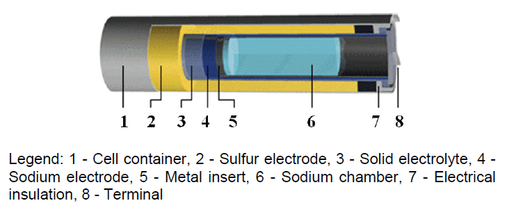
During discharge, as positive Na+ ions flow through the electrolyte and electrons flow in the external circuit of the battery producing about 2 volts. This process is reversible as charging causes sodium polysulfides to release the positive sodium ions back through the electrolyte to recombine as elemental sodium. This hermetically sealed battery is kept at approximately 300°C and is operated under conditions such that the active materials at both electrodes are liquid and the electrolyte is solid. At this temperature, since both active materials react rapidly and because the internal resistance is low, the NAS battery performs well. Because of reversible charging and discharging the NAS battery can be used continuously. Efficiency of NAS battery cells is about 89%. [2]

Redox Flow Batteries

The reduction-oxidation (Redox) flow batteries are considered highly prospective, as these are able to store large amounts of electric power. For this purpose, the ability of some chemical elements (e.g. vanadium) to have more valence states is utilized. The core of this system comprises a reversible reduction-oxidation cell to accommodate the transformation of electrical energy into chemical energy, bound within the electrolyte. These Redox batteries allow for continuous exchange of electrolyte. This ensures their continuous operation until the electrolyte supply has been used up. Electrolytes circulate within two circuits separated by the ion exchanger membrane inside the very cell. The cell interior provides for oxidizing of one form of the electrolyte upon electrochemical process, with the other one being subject to reduction due to the electric current fed or drained into the external electric circuit with the use of electrodes (see Figure 2).

Fig.2 Diagram of Redox flow battery working principle [4]

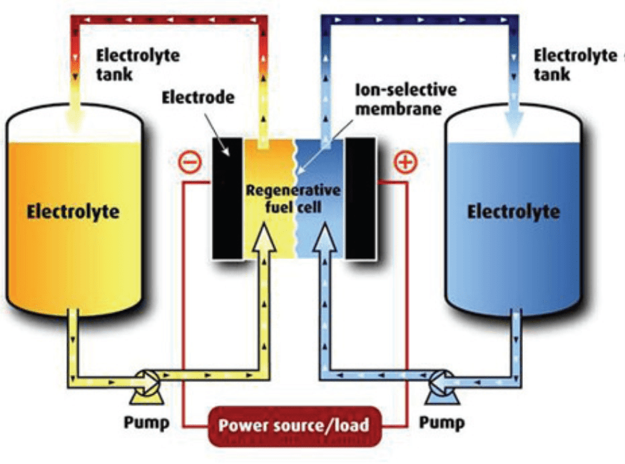
The storage capacity is determined by the amount of electrolyte in store tanks, while the actually achievable volume energetic density of electrolyte for a full charging (discharging) cycle is listed within the range of 15 to 25 kWh/m3. The unit does not show any performance or capacity reduction after more than 12 thousand charging cycles, the estimated life span of membranes is approximately 15 years. [3]

Supercapacitors

Also referred to as super condensers, are actually electrolytic capacitors with high capacity of thousands of F (Farad) and the ability for rapid charging and discharging. The electrodes are made from special materials as the micro-porous active carbon, which features extreme surface properties of up to 2000 m2/g and the gap of several nanometres between particular charged layers. These electrodes are separated with the polypropylene foil, the space within is filled with liquid electrolyte. The operation voltage is approx. 2,5V. Any higher voltage can be achieved by series setup of basic cells. The low internal resistance value enables for rapid discharge, the excellent performance provided by super capacitor achieves the values of several kW per 1kg of weight. Their electric parameters are maintained even under low temperatures down to -40°C. Supercapacitors represent ideal units to be used in applications with the need for peak current supply for a limited period of time. Their commercial utilisation has been launched recently only. [3]

High-Speed Flywheels

There are still the more common low-speed flywheels (rotating by up to approx. 7.000 rpm) provided with steel rotors. The very strong composite materials allow for development of light high-speed flywheels with the maximum speed up to approx. 50.000 rpm. To reduce the friction produced, the rotor will be housed within vacuum with magnetic uplift. The rotor also comprises permanent magnets, which help with its initial roll-up or generate current within coils.

These units also feature sophisticated electronics to ensure the safe and maintenance free operation. The contemporary flywheels can provide the performance from several kW up to approx. 1 MW. Their advantage lies in the optional operation of several units in parallel. A steel flywheel can provide approx. 200 kW of backup power within a 3-phase 400V network with the revolutions range of 7.700 – 4.000 rpm. Any such unit can be also operated separately as a short-term backup or a component within a larger system. [5]

Superconducting Magnetic Energy Storage (SMES)

The superconducting magnetic electrical energy storage units enable the rapid absorption and supply of power without any limitations or losses. Energy is stored within the magnetic field of coil bearing current, this coil being housed within a cryostat. Such coil is made from a superconductor in order to eliminate any resistance losses. However, there are power losses incurred during operation of the cooling unit, which maintains the coil superconductor below the critical temperature level.

The SMES system helps to store up to thousands of MWh and it can be used to balance peaks of electric power take-off. The very superconducting coil, depending on the size and method of use, can be made of a solenoid toroid. The superconductor energy accumulator might be the alternate solution for electrical energy storage in forthcoming years. However the need for cooling to preserve its operational temperature below critical level makes this unit costly compared to other technologies. [5]

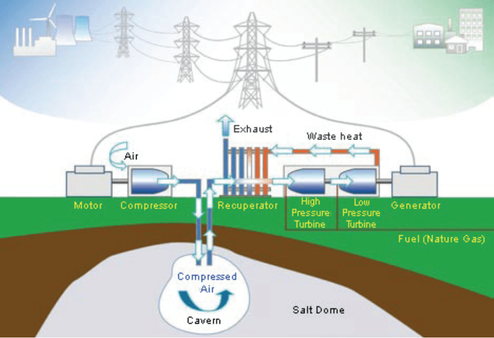
CAES (Compressed Air Energy Storage) System

This is a compressed air accumulator linked with a turbine to supply power during take-off peaks within the network as needed. It is a peaking gas turbine power plant that consumes less than 40% of the gas used in conventional gas turbine to produce the same amount of electric output power. This is because, unlike conventional gas turbines that consume about 2/3 of their input fuel to compress air at the time of generation, CAES pre-compresses air using the low cost electricity from the electrical power system at off-peak times and utilizes that energy later along with some gas fuel to generate electricity as needed. The compressed air is often stored in appropriate underground mines or caverns created inside salt rock (see Figure 3). The CAES technology is still used very rarely in global commercial projects. [6]

Fig.3 Principle of CAES system [6]
Hydrogen Storage System

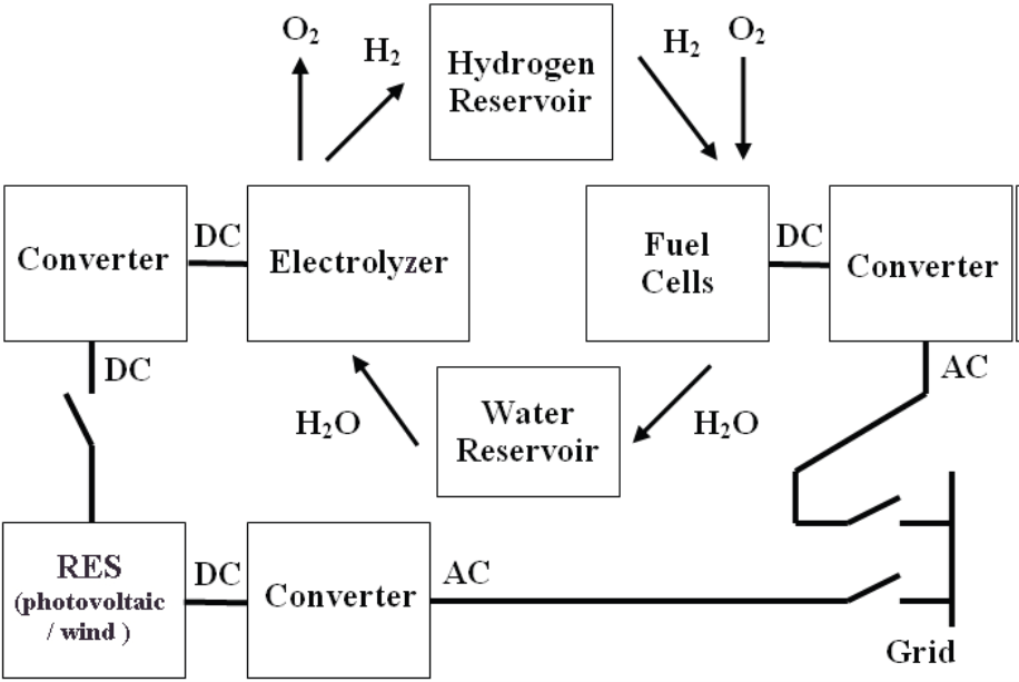
The main parts of this system comprise the hydrogen generator, the so called “electrolyzer”, the magazine to hold the hydrogen produced, the demineralised water magazine and the hydrogen fuel cells. Further components necessary include the semiconductor invertors, compressors and vents. The cooperation between the hydrogen system and the non-controlled RES is based on the principle that the power produced by RES will be used to produce hydrogen within the period of lower EPS workload and this hydrogen will be stored. The hydrogen in storage will be later used in fuel cells, consumed during production of electric energy in the period associated with demand for electric energy by EPS. Figure 4 shows the diagram of hydrogen system.

Pumped-Storage Hydro Plant

A pumped-storage hydro plant (PSHP) represents a system able to store large amounts of electric energy. PSHP units are used to cater for peak demands for electric energy within EPS. Apart from the latter, these units also play their unique role within the control of output of the national energetic system in terms of emergency reserve. Their installed capacity within the territory of Czech Republic amounts to 1.175 MW. The PSHP serves for storage of electric energy using the potential gravity energy of water. The unit comprises of two reservoirs, whereas one of them is placed below the other. These reservoirs are linked with gravity piping of large diameter. During the period of power surplus within the EPS (at night), this power is used to pump the water from the bottom reservoir up into the top one. Once the ESP has developed a demand for large amount of peak power, this water will be subject to controlled discharge from the top reservoir down into the bottom one via the hydro plant turbine. This storage system is costly and requires significant landscape adaptations. The rate of efficiency of this pumping cycle is approx. 75%.

Storage Systems Benchmark

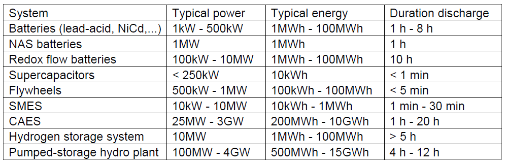
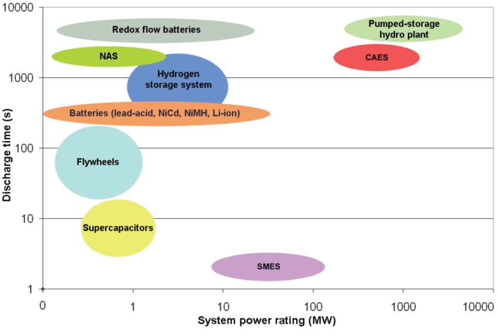
The storage systems described above have been grouped within the Table 1 to allow for proper comparison of basic parameters. Figure 5 then shows a graphic comparison of these systems, in order corresponding to their power rating and the discharge time.

Laboratory Research into Hydrogen Storage System

The storage system based on the hydrogen technology seems to be very prospective with regard to cooperation with the non-controlled RES. There is currently a research focused on this technology in progress, together with examination of its practical application. This research also involves our laboratory at the Department of Electrical Power Engineering, VŠB – TU Ostrava, concerned with sophisticated experimental laboratory implementation of the model hydrogen system for storage of electric energy produced by photovoltaic panels. Further detailed information about these panels is contained within other paper by authors dealing with the issue of photovoltaic power plant operation within the territory of the Czech Republic.

Our research concerns testing and measuring of particular components of the hydrogen system designed in order to optimise their operation to provide reliable, safe and highly efficient units. See the block diagram in Figure 4.

Table 1. Basic parameters of storage systems [7]

.
Fig.4. The hydrogen storage system diagram
Fig.5. Graphic comparison of energy storage systems [7]
Electrolyzer

Electrolyzer producing hydrogen is the first one of the most important parts of the entire hydrogen system. The process of electrolysis helps use the energy to decompose water to the very elements: hydrogen and oxygen. The electrolyzer comprises a series of cells equipped with positive and negative electrodes respectively, these are dipped in water. The level of conductivity is achieved by addition of hydrogen or hydroxyl ions (hydroxides), the most common form is the alkali potassium hydroxide (KOH). The amount of hydrogen produced depends on the flow density. The current electrolyzers feature energetic efficiency between 65 and 80 %. We use the Hogen GC600 electrolyzer comprising of electrodes and the gas separator to provide for separation of hydrogen produced from oxygen.

Electrolyzers of this kind use the sulhponated tetrafluorethylene (Nafion) to substitute the liquid electrolyte. The input of this electrolyzer is 1.100W, its operation temperature ranges around 85°C, the volume of hydrogen produced equals to 0,6 l/min (high purity: 99,999%), the output pressure of hydrogen reaches up to 13,8 bar. The source of energy used for decom-position of water is represented by photovoltaic panels.

Despite the low specific density, hydrogen has the highest ratio of energy to weight among all the fuels. As far as gases are concerned, its density is the lowest possible and it also features the second lowest boiling point of all the known substances. These properties then determine the options for its storage. [8]

It can be stored as a highly compressed gas, as a liquid in cryogenic magazines or as a bonded gas (e.g. in metal-hydrides). The storage of hydrogen in gaseous form requires large magazine volumes and high compression. High pressure hydrogen storage units represent the most common method used. If liquid, the hydrogen can be stored below its boiling point only, which is equal to 20 K (-253 °C). Owing to the latter, the liquefying of hydrogen is a strongly energy demanding process. The storage systems with metal-hydrides are based on the principle of easy absorption of gas by certain materials under high pressure and moderate temperatures. These substances would then release hydrogen, when beating heated under low pressure and relatively high temperatures. [8]

We use metal-hydride bottles and pressure cylinders for laboratory research.

PEM Fuel Cell

A fuel cell is a device, which uses the electrochemical reaction to transform chemical energy held by the fuel (hydrogen), aided by the oxidizing agent, to electric power, water and heat. This transformation occurs within catalytic reactions on electrodes and it is mainly based on reversed principle of water electrolysis. This efficiency of this energy production process is up to 60 % (under laboratory conditions), the real value would then be between 35 and 50 % (depending on the load and fuel cell type). This efficiency is mainly ensured by the method of energy transformation being direct with no intermediate levels (heat and mechanic energy), unlike in case of steam power plants, combustion engines or turbines, for example. [9]

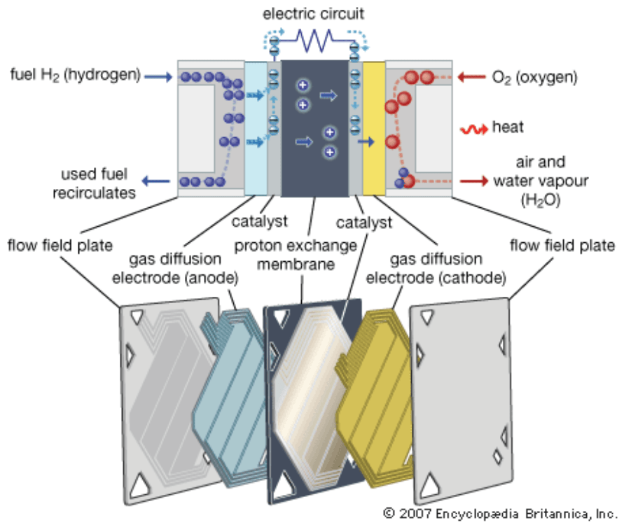
There are currently six types of fuel cells under development and these differ by electrolyte composition, operation temperatures and the type of fuel used. Proton Exchange Membrane (PEM) fuel cells are cells with polymeric electrolyte membrane known for their high conductivity, which allows for their design of light weight and reasonable dimensions. These cells use the electrolyte able to conduct H+ ions from anode towards cathode. The electrolyte used will usually be perfluorinated polymer of the sulphonic acid inserted between two electrodes impregnated with catalyser. PEM usually work under temperatures between 50 and 100 °C and the pressure of 1 to 2 bar. Figure 6 shows PEM fuel cell principle. These fuel cells provide for the chemical reaction listed below:

  • Anode: 2 H2 ⇒ 4 H+ + 4 e
  • Cathode: O2 + 4 e + 4 H+ ⇒ 2 H2O

The H+ ions pass through the electrolyte, from the anode towards cathode, whereas electrons are forced to pass from the anode towards cathode through the external electric circuit. Water produces by the cell, aggregated on the cathode, must be drained out of the cell continuously. [9]

Fig.6. PEM fuel cell principle

The output of both described devices is directly dependant on the surface of electrode with main impact on their total cost. The total amount of the accumulated energy depends on the size of hydrogen container and the output from RES, i.e. the photovoltaic system.

The stage of testing of specific parts of the storage system built will be followed by their linkage to form a working system. The main components of this system comprise the renewable energy source based on the photovoltaic technology, the hydrogen production block with electrolyzer and the container for storage of hydrogen produced and the production electro-block with fuel cell modules and semi-conductor invertors, current inverters respectively.

Measurements on Fuel Cell System

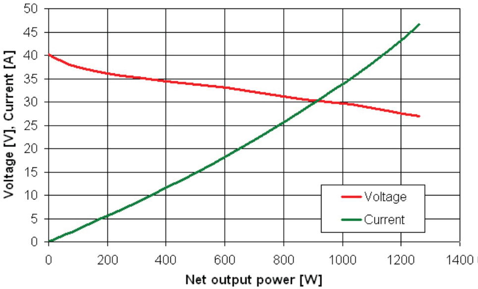
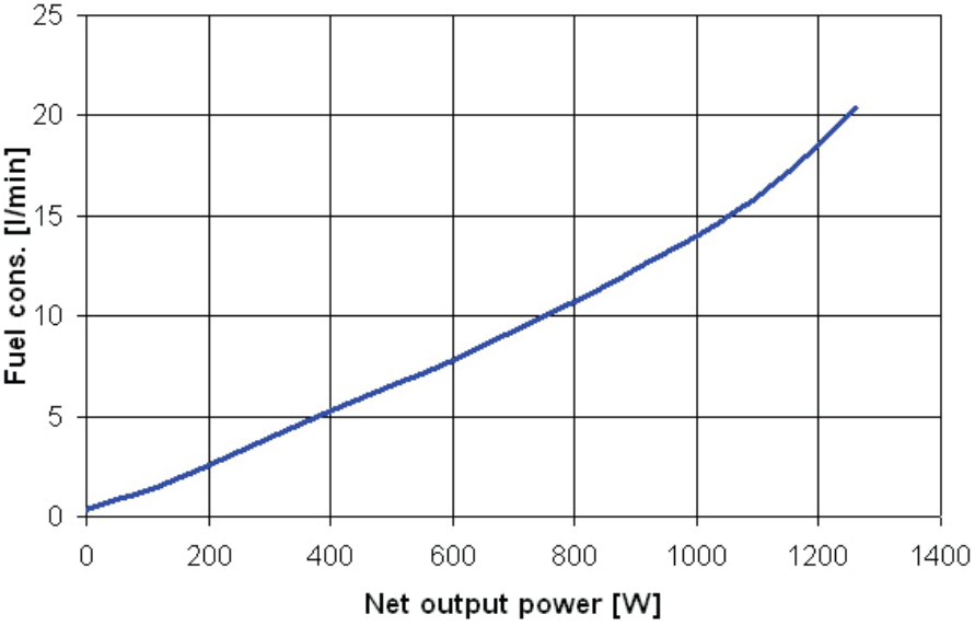
Our research laboratory is equipped with two low-temperature fuel cells Nexa Power Module (Ballard Power Systems Inc.). Rated power output of one Nexa Module is 1200 W. They are being tested in various operating conditions. The measuring procedure consists of cyclic measurements of the load characteristics of NEXA, whereas the system is connected to the distribution network via inverter, in between these measurements, to supply the electric energy. The load characteristics you can see on Figure 7. That is demonstrated in the fuel consumption graph (see Figure 8). This fuel consumption has been determined from the flow meter after the so called purge of cells. This purge deprives cells of impurities and water on regular basis, as those are accumulated on electrode surfaces to intercept the electrochemical reaction.

Fig.7. Load characteristics of NEXA
Fig.8. Fuel consumption of NEXA
Fig.9. Stack current and voltage during normal operation

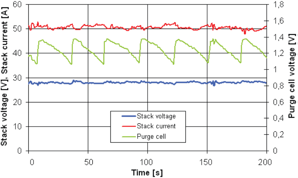
The frequency of purges rises with the increase of cell power output. The NEXA power system measures the voltage over two cells within a stack (fuel cells connected in series), the so called purge cells, to conduct the purging of fuel cells with hydrogen once the voltage has dropped below a certain level to restore the higher voltage in cells again (see Figure 9).

The fuel used for cleaning is drained out of the system unused for the reaction within fuel cells. Yet it shall be included into the overall consumption. That was the reason why we conducted accurate measurements within the system under electronic load at the particular nominal power output, one hour for each. The consumption was determined using a flow meter with an integration member. The Figure 9 shows the normal curve of stack values during the operation.

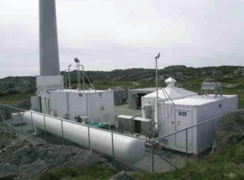
Wind-Hydrogen Power Plant

This is a complex combining a wind power plant and the hydrogen storage system based on the Utsira island at the Western coast of Norway. The entire complex is fully autonomous. The insular power distribution network supplies electric power to every household on the island, whose annual consumption amounts to approx. 200 MWh. Figure 11 shows the photograph of the entire complex with the evident tube of wind power plant with the installed capacity of 600kW, with the container and electrolyzer providing the installed capacity of 48kW situated below, with the hydrogen production capacity of 10m3/h, and the compressor with the output of 5,5kW. The photograph shows the container for 2.400 m3 of hydrogen compressed at the ratio of 200 bar. There are containers housing he fuel cell providing the output of 55kW on the right hand side. Both the electrolyzer and the fuel cell are of PEM type. [10]

When the wind turbine at Utsira is running at optimum level, it will produce more energy than the consumption is.

Fig.10 Photograph of power plant at Utsira [10]
Fig.11. Operation of Utsira power plant – Low wind mode [10]

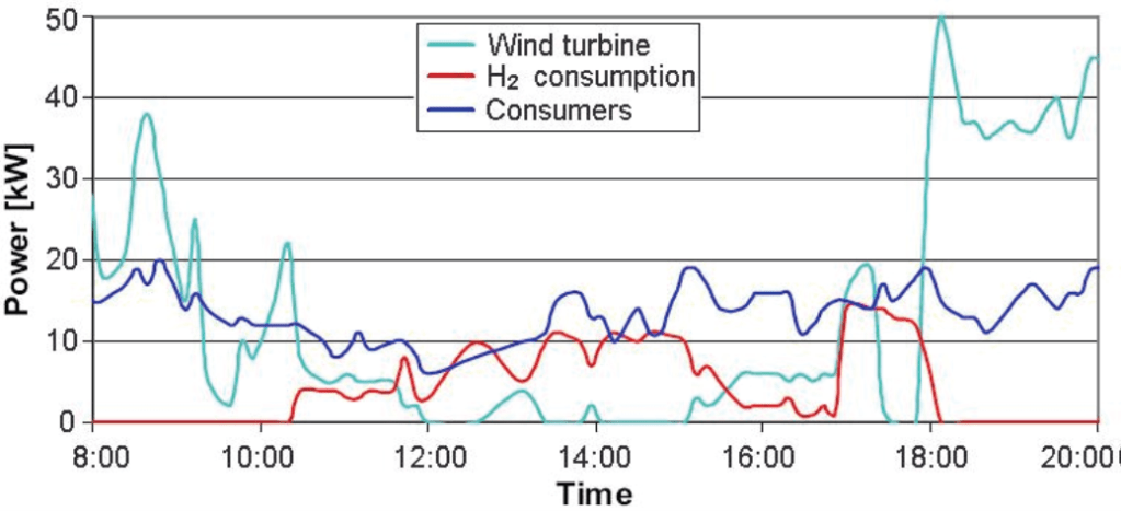
The surplus energy is used to produce hydrogen through water electrolysis. The hydrogen produced is compressed and stored in a gas storage vessel and is available when needed. Under circumstances when the wind turbine is not in operation (i.e. when there is too little or too much wind) the hydrogen is used in a fuel cell and a combustion engine-generator unit to produce power. Example of operation of power plant at Utsira is illustrated on Figure 11. On this graph you can see that the wind power decreases and cannot supply the demand. In this period the fuel cell and engine-generator are started and are balancing the load. [10]

Conclusion

The accumulation of electric power, especially the power gained from the photovoltaic and wind power plants, is of significant importance with respect to their operation in relation with the electric power system. Those are sources providing variable and unreliable supply of electric power over time, which has negative impact on the operation of the electric power system. The accumulation of electric power produced by those units can contribute towards substantial reduction of the control power, which shall be maintained within the electric power system. There is a whole range of suitable accumulation technologies available. However, their practical application in relation with the RES mentioned is still subject to research in progress.

Redox flow batteries are seen as a prospective technology as their accumulation capacity is limited by the amount of liquid electrolyte within only, i.e. the size of magazines used. These can be used to build large accumulation facilities within electric power networks. Construction of a CAES will be mainly dependant on the local geological conditions. This system is very complex from the implementation point of view, same as the pumped-storage hydro plant. There are very few CAES pilot projects in operation only.

The hydrogen system can be used to provide for accumulation of electric power in large amounts as well.

The higher cost of implementation might still represent certain problems as those are determined by the cost of materials used. However, this technology is subject to continuous dynamic development, whose future lies not only in stationary applications yet even in mobile projects. The accumulation system mentioned above can be supplemented with flywheels or super capacitors able to cater for short-term fluctuations in supply of electric power.

This work is supported by The Ministry of Education, Youth and Sports of the Czech Republic, project CEZ MSM6198910007″.

REFERENCES

[1] Cenek, M., Accumulators: from principle to practise. FCC Public, Praha, Czech Republic, 2003
[2] NAS batteries [online],
[3] Hradílek, Z., Moldřík, P., Šebesta, R., Storage of Electric Energy Gained from Renewable Sources. Proceedings of AsiaPES, 2009, Beijing, China
[4] About Flow battery [online],
[5] Moldřík, P., Hradílek, Z., Chválek, R., Research of Energy Storage Gained from Renewable Sources. Proceedings of Elnet, 2009, Ostrava, Czech Republic
[6] CAES system [online],
[7] De Boer, P., Raadschelders, J., Flow batteries. Leonardo Energy website [online],
[8] Hradílek, Z., Chválek, R., Research accumulation of energy from renewable energy sources in fuel cells. Proceedings of EPE, 2009, Kouty nad Desnou, Czech Republic
[9] Larminie, J., Fuel Cell Systems Explained. John Wiley and Sons Inc., 2003, Chichester, United Kingdom
[10] Nakken, T., The Utsira wind-hydrogen system: operational experience. Proceedings of EWEC, 2006, Athens, Greece


Authors: prof. Ing. Zdeněk Hradílek, DrSc., Ing. Petr Moldřík, Ph.D., Ing. Roman Chválek, Technical University of Ostrava, Faculty of Electrical Engineering and Computer Science, Department of Electrical Power Engineering, ul. 17. listopadu 15, 708 33 Ostrava – Poruba, Czech Republic, E-mail: zdenek.hradilek@vsb.cz; petr.moldrik@vsb.cz; roman.chvalek@vsb.cz


Source & Publisher Item Identifier: PRZEGLĄD ELEKTROTECHNICZNY (Electrical Review), ISSN 0033-2097, R. 87 NR 2/2011

Prospective Short Circuit Test and Prospective Fault Current Test (PSC & PFC TEST)

Published by Carelabs, Carelabs (Carelabz) is authorized provider of Electrical Installation’s Study, Analysis, Inspection, and Certification services in UAE. Website: carelabz.com


Prospective  Short  Circuit (PSC) and Prospective Fault  Current (PFC) are both intended to calculate the highest current that will stream within a fault loop path during the occurrence of an electrical flaw as needed by rules.   

The  Prospective Short Circuit Current (PSC) is the utmost current that could flow between Line and Neutral conductors on a single-phase supply or between Line conductors on a three-phase supply. A PSC test calculates the current that will flow in the event of a short circuit fault between the live conductors. That is, Line and Neutral on a single-phase installation or Line to Line/ Line to Neutral on a three-phase installation.  

Prospective Fault Current (PFC) is the common term used for the highest amount of current that will stream under fault conditions. The PFC will continuously be the highest at the source of the installation as the impedance/resistance is always the lowest there. So as a regulation, if it’s not too extreme at the mains it will be fine everywhere else. This is because it will decrease due to the increase in resistance as we move further away from the origin. (ohms law I = V/R). 

Because of the type of dissimilar supplies, you would assume to find a PSC value greater than a PFC value on both TT and TN-S systems, yet on a TNC-S system both the PFC and PSC readings should be same.

What is done During PFC and PSC Tests? 

PSC is decided by the voltage and impedance of the supply system. It’s far of the order of some thousand amperes for a well-known domestic mains electrical set up, but can be as little as a few milliamperes in a separated extra-low voltage (SELV) device or as excessive as hundreds of heaps of amps in huge industrial strength systems 

PFC is conducted at the source of the installation, like the main switch or at other switchgear connected straight to the tail from the electricity distributor’s metering device. Where a calculation is made at a point in the installation other than the source, such as a piece of switchgear served by a distribution circuit, it would not be the highest value for the installation.  

Particular guardianship should be exercised during the testing summons, as flaw conditions are most severe at the origin of an installation, where this test is performed. The earthing conductor, main protective bonding conductors and circuit protective conductors should all be connected as for normal operation during these trials, because the presence of these and any other latitude ways to earth may reduce the impedance of the earth flaw loop and so increment the level of prospective fault current. 

PSC will be greater than the PFC. Prospective fault current and short circuit current of a circuit is automatically calculated when making a loop impedance test. The calculation uses a nominal circuit voltage, not the actual circuit voltage. 

Why PSC and PFC are Done? 

PFC and PSC test is necessary for choosing the correct protective device for the circuit because it’s going to carry the maximum fault current flowing in a circuit. Regulation 612.11 of BS 7671 requires that the prospective fault current under both short circuit and earth fault conditions be determined for every relevant point of the installation. 

How is PSC and PFC Performed? 

The minor supply voltage used in the calculation is automatically chose depending on the real circuit voltage. The instrument uses the following voltage values: 

Prospective Short Circuit Test Procedure 

PFC tester or the Prospective short circuit function of a multifunctional tester such as the Megger 1553 is chosen, and we make sure that the supply is ON, but the Main Switch is in OFF position. 

The test leads are joined on the incoming side of the Main Switch, one test lead on Line and another on the Neutral terminals of the Main Switch. 

TEST switch is pushed and a note of the value (kA) is made. 

For three phase installations each phase is tested separately and the measured reading (test between Line 1 and Neutral, then Line 2 and Neutral and last Line 3 and Neutral) is doubled. 

Some test meters need that the third (usually green) lead to be connected on the Neutral during this test. Please refer to the test meter manufacturer’s instruction. 

Prospective Fault Current Test Procedure 

We use PFC tester or select the PFC function of a multifunctional tester such as the Megger 1553, and it has to be made sure that the supply is ON, but the Main Switch is in OFF position. 

Next, we connect the test leads on the Line and Neutral terminals of the Main Switch, as well as on the Earth terminal. 

The TEST switch is pushed and we make note of the reading (kA).
For three phase installations each phase is checked separately and the measured reading is doubled (L1 – N – CPC, L2 – N – CPC, L3 – N – CPC). 

Having obtained these values by the measurements described above, we will select the highest value and write it down on the Electrical Installation Certificate as the value of PFC. 

The value of PFC obtained is compared with the breaking capacity of all the protective devices within the installation. The breaking capacity of the protective devices should be greater than the value of PFC. 

Benefits of PSC and PFC Tests

  • They give accurate results as its live testing.
  • The testing is simple and not much calculations are needed. 
  • Increased safety for employees and third parties.
  • Decreased Insurance Premiums.
  • Asset Data management and tracking systems. 
  • Small repairs of equipment made on-site to reduce down time.

Source URL: https://carelabz.com/prospective-short-circuit-test-prospective-fault-current-test/#:~:text=Prospective%20Fault%20Current%20(PFC)%20is,is%20always%20the%20lowest%20there.

General Reference – Utility Capacitor Switching

Published by Electrotek Concepts, Inc., PQSoft Case Study: General Reference – Utility Capacitor Switching, Document ID: PQS0302, Date: January 10, 2003.


Abstract: The application of utility capacitor banks has long been accepted as a necessary step in the efficient design of utility power systems. Also, capacitor switching is generally considered a normal operation for a utility system and the transients associated with these operations are generally not a problem for utility equipment. These low frequency transients, however, can be magnified in a customer facility (if the customer has low voltage power factor correction capacitors) or result in nuisance tripping of power electronic based devices, such as adjustable-speed drives.

Capacitor energizing is just one of the many switching events that can cause transients on a utility system. However, due to their regularity and impact on power system equipment, they quite often receive special consideration.

INTRODUCTION

The application of utility capacitor banks has long been accepted as a necessary step in the efficient design of utility power systems. Also, capacitor switching is generally considered a normal operation for a utility system and the transients associated with these operations are generally not a problem for utility equipment. These low frequency transients, however, can be magnified in a customer facility (if the customer has low voltage power factor correction capacitors) or result in nuisance tripping of power electronic based devices, such as adjustable-speed drives (ASDs). Capacitor energizing is just one of the many switching events that can cause transients on a utility system. However, due to their regularity and impact on power system equipment, they quite often receive special consideration.

Transient overvoltages and overcurrents related to capacitor switching are classified by peak magnitude, frequency, and duration. These parameters are useful indices for evaluating potential impacts of these transients on power system equipment. The absolute peak voltage, which is dependent on the transient magnitude and the point on the fundamental frequency voltage waveform at which the event occurs, is important for dielectric breakdown evaluation. Some equipment and types of insulation, however, may also be sensitive to rates of change in voltage or current. The transient frequency, combined with the peak magnitude, can be used to estimate the rate of change.

There are a number of transient related concerns that are generally evaluated when transmission and distribution shunt capacitor banks are applied to the power system. These concerns include insulation withstand levels, switchgear ratings and capabilities, energy duties of protective devices, and system harmonic considerations. In addition, these considerations need to be extended to include customer facilities due to the increased use of power electronic based end-user equipment. Applications concerns often evaluated include:

− overvoltages associated with normal capacitor energization.
− open line/cable end transient overvoltages.
− phase-to-phase transients at transformer terminations.
− voltage magnification at lower voltage capacitor banks (including customer systems).
− arrester duties during restrike events.
− current-limiting reactor requirements.
− system frequency response and harmonic injection.
− impact on sensitive customer power electronic loads.
− ferroresonance and dynamic overvoltage conditions.

Power quality symptoms related to utility capacitor switching include customer equipment damage or failure, nuisance tripping of ASDs or other process equipment, transient voltage surge suppressors (TVSS) failure, and computer network problems.

CAPACITOR BANK ENERGIZATION

Transient characteristics are dependent on the combination of the initiating mechanism and the electric circuit characteristics at the source of the transient. Circuit inductances and capacitances – either discrete components such as shunt capacitance of power factor correction banks or inductances in transformer windings, or stray inductance or capacitance because of proximity to other current carrying conductors or voltages – are responsible for the oscillatory nature of transients. Natural frequencies within the power system depend on the system voltage level, line lengths, cable lengths, system short circuit capacity, and the application of shunt capacitors.

Characteristics of Energizing an Isolated Capacitor Bank

Energizing a shunt capacitor bank from a predominantly inductive source results in an oscillatory transient that can approach twice the normal system peak voltage (Vpk). Figure 1 illustrates the simplified equivalent system for the energizing transient. The characteristic frequency (fs) of this transient is given by:

.

and the peak inrush current (Ipk) is determined using:

.

where:

[example]
fs = characteristic frequency (Hz) = [379 Hz]
Ls = positive sequence source inductance (H) = [17.53mH]
C = capacitance of bank (F) = [10.03μF]
fsystem = system frequency (50 or 60 Hz) = [60 Hz]
Xs = positive sequence source impedance (Ω) = [6.61 Ω]
Xc = capacitive reactance of bank (Ω) = [264.50 Ω]
MVAsc = three-phase short circuit capacity (MVA) = [2000 MVA]
MVAr = three-phase capacitor bank rating (MVAr) = [50 MVAr]
ΔV = steady-state voltage rise (per-unit) = [2.5%]
Vpk = peak line-to-ground bus voltage (V) = [93897.11 V]
Zs = surge impedance (Ω) = [39.35 Ω]

Relating the characteristic frequency of the capacitor energizing transient (fs) to a steady-state voltage rise (ΔV) design range provides a simple way of quickly determining the expected frequency range for utility capacitor switching. For example, a 60 Hz system with a design range of 1.0% to 2.5% would correspond to characteristic frequency range of 380 to 600 Hz. For a shunt capacitor bank on a high voltage bus, transmission line capacitance and other nearby capacitor banks cause the energizing transient to have more than one natural frequency. However, for the first order approximation, the equation above [1] can still be used to determine the dominant frequency.

Figure 1 – Equivalent Circuit for Capacitor Energizing

Because capacitor voltage cannot change instantaneously (remembering that i(t)=Cdv/dt), energization of a capacitor bank results in an immediate drop in system voltage toward zero, followed by an oscillating transient voltage superimposed on the 60 Hz fundamental waveform. The peak voltage magnitude depends on the instantaneous system voltage at the instant of energization, and can reach 2.0 times the normal system voltage (Vpk – in per-unit) under worst-case conditions. The voltage surge is at the same frequency as the inrush current (Ipk) and rapidly decays to the system voltage.

For a practical capacitor energization without trapped charge, system losses, loads, and other system capacitances cause the transient magnitude to be less than the theoretical 2.0 per-unit. Typical magnitude levels range from 1.2 to 1.8 per-unit and typical transient frequencies generally fall in the range from 300 to 1000 Hz. Figure 2 illustrates an example (measured) distribution system capacitor energizing transient.

Figure 2 – Typical Distribution Bus Voltage during Capacitor Energizing

Energizing an ungrounded-wye capacitor bank can result in slightly higher transient overvoltages because of unequal pole closing. In general, the transient overvoltages associated with normal closing are similar to those for grounded banks.

Characteristics of Energizing Back-to-Back Capacitor Banks

Energizing a shunt capacitor bank with an adjacent capacitor bank already in service is known as “back-to-back” switching. High magnitude and frequency currents, illustrated in Figure 3, will flow between the banks when the second bank is energized. This current must be limited to acceptable levels for switching devices and current transformer burdens. Generally, series reactors are used with each bank to limit the current magnitude and frequency, although pre-insertion resistors/inductors may be used with some types of switches.

The frequency and magnitude of the inrush current during back-to-back switching depends upon the size of the discharging capacitor bank, the impedance of the discharging loop, and the instantaneous capacitor bank terminal voltage at the time of contact closure. The impedance of the discharging loop is determined by the inductance between the banks rather than the system inductance (Ls). The magnitude of the inrush current is therefore much higher than for the isolated bank energization (Ipk). Typically, the inrush current lasts for only a fraction a power frequency cycle.

This high-frequency inrush current may exceed the transient frequency momentary capability of the switching device (e.g. ANSI C37.06-1987) as well as the I2t withstand of the capacitor fuses. It may also cause false operation of protective relays and excessive voltages for current transformers (CTs) in the neutral or phase of grounded-wye capacitor banks. The current must be evaluated with respect to the transient frequency momentary capability (close and latch) rating of the switch, as well as the I2t withstand of the capacitor fuses. Switch manufacturers should be consulted for the appropriate current (Ipk) and frequency (f) ratings of the device. High frequency substation ground mat currents may be controlled by connecting the two neutral points together and grounding with a single connection to the grid.

Figure 3 – Example Distribution Feeder Current during Back-to-Back Switching

Solutions to excessive inrush currents usually involves:

− adding current-limiting reactors to decrease the peak current and frequency of the oscillatory inrush current.
− adding pre-insertion resistors or inductors to the switching device.
− adding synchronous closing control to the switching device.
− selecting component ratings (e.g. breaker, CT burdens, etc.) to withstand the inrush current characteristics.

OVERVOLTAGE MITIGATION

Devices for capacitor switching transient control either attempt to minimize the overvoltage (or overcurrent) at the point of application, or limit (clip) the overvoltage at local and remote locations. These devices include:

− a) synchronous closing control (also known as zero voltage closing)
− b) pre-insertion devices (resistors and/or inductors)
− c) fixed inductors
− d) MOV arresters

Previous research has suggested that the effectiveness of these control methods is system dependent, and that detailed analysis is required to select the optimum control scheme. While often justifiable for large transmission applications, transient analysis of distribution capacitor applications is rarely performed, and in general, banks are installed without transient overvoltage control. Each of these methods has various advantages and disadvantages in terms of transient overvoltage reduction, cost, installation requirements, operating/maintenance requirements, and reliability.

Timing Control

Synchronous closing is independent contact closing of each phase near a voltage zero, as illustrated in Figure 4. To accomplish closing at or near a voltage zero (avoiding high prestrike voltages), it is necessary to apply a switching device that maintains a dielectric strength sufficient to withstand system voltages until its contacts touch. Although this level of precision is difficult to achieve, closing consistency of ±0.5 milliseconds should be possible. Previous research has indicated that a closing consistency of ±1.0 millisecond provides overvoltage control comparable to properly sized pre-insertion resistors. The success of a synchronous closing scheme is often determined by the ability to repeat the process under various (system and climate) conditions. Adaptive, microprocessor-based control schemes that have the ability to “learn” from previous events address this concern. The primary benefits of this capability are the control’s ability to compensate for environmental factors and the increased reliability (less maintenance) that can be achieved

Grounded capacitor banks are controlled by closing the three phases at three successive phase-to-ground voltage zeros (60° separation). Ungrounded banks are controlled by closing the first two phases at a phase-to-phase voltage zero and then delaying the third phase 90 degrees (phase-to-ground zero).

Figure 4 – Concept of Synchronous Closing Control

Pre-insertion Devices

A pre-insertion impedance (resistor or inductor) provides a means for reducing the transient currents and voltages associated with the energization of a shunt capacitor bank. The impedance is “shorted-out” (bypassed) shortly after the initial transient dissipates, thereby producing a second transient event. The insertion transient typically lasts for less than one cycle of the system frequency. The performance of pre-insertion impedance is evaluated using both the insertion and bypass transient magnitudes, as well as the capability to dissipate the energy associated with the event, and repeat the event on a regular basis. The optimum resistor value for controlling capacitor energizing transients depends primarily on the capacitor size and the source strength.

Fixed Inductors

Fixed inductors have been used successfully to limit inrush currents during back-to-back switching. Typically the value of these inductors is on the order of several hundred microhenries. In addition, inductors provided for outrush (into a nearby fault) current control may be applied, and are typically 0.5 – 2.0 millihenries. Previous research indicates that these fixed reactors do not provide any appreciable transient overvoltage reduction.

MOV Arresters

Metal oxide varistors (MOVs) can limit the transient voltages to the arrester’s protective level (maximum switching surge protective level, typically 1.8 – 2.5 per-unit) at the point of application. The primary concern associated with MOV application is the energy duty during a restrike event. Although a rare occurrence, a switch restrike generally results in the highest arrester duty for arresters located at the switched capacitor. In addition, remote arresters (including low voltage customer applications) may be subjected to severe energy duties if voltage magnification occurs. This condition could be especially troublesome for distribution systems if SiC arresters remain in service.

POWER QUALITY CONSIDERATIONS

Voltage Magnification:

Voltage magnification occurs when a transient oscillation, initiated by the energization of a utility (transmission or distribution) capacitor bank, excites a series resonance formed by a lower voltage system. The result is a higher overvoltage at the lower voltage bus. Previous analysis has indicated that the worst magnified transient occurs when the following conditions are met (refer to Figure 5):

− The size of the switched capacitor bank is significantly larger (>10) than the lower voltage (often customer power factor correction) bank (i.e. 50MVAr versus 1.8MVAr ≈ 28).

− The energizing frequency (fs) is close to the series resonant frequency formed by the step-down transformer and the power factor correction capacitor bank (f2) (i.e. 465Hz @ 230kV bus vs. 440Hz @ 13.2kV bus).

− There is relatively little damping (resistive) provided by the low voltage load (typical industrial plant configuration – primarily motor load).

Distribution system overvoltages, resulting from transmission capacitor bank energization, may be sufficient to spark-over SiC arresters. MOV arresters should be capable of withstanding the event, however this should verified using computer simulations and/or TNA analysis. Low voltage customer systems may be exposed to transient overvoltages (illustrated in Figure 6) between 2.0 and 4.0 per-unit, (previously determined by computer simulations and in-plant measurements) and these overvoltages may occur over a wide range of low voltage capacitor sizes (note that the low voltage capacitor must exist for magnification to occur). Typically, the transient overvoltages will simply damage low-energy protective devices (MOVs) or cause a nuisance trip of a power electronic-based device. However, there have been several cases when complete failure of customer equipment (single process device) has occurred.

Important system variables to consider when analyzing this phenomenon include:

− Switched capacitor bank size
− Lower voltage capacitor bank size and location
− System loading
− Transformer characteristics
− Circuit breaker characteristics (closing resistors/inductors, closing control, etc.).
− Arrester size(s), rating(s), and location(s)

Figure 5 – System Diagram for Voltage Magnification Condition
Figure 6 – Transient Overvoltages during Voltage Magnification

A number of utilities and their customers have evaluated and tested several possible solutions to the voltage magnification problem, including:

− Detuning the circuit by changing capacitor bank sizes, moving banks, and/or removing banks from service (utility and/or customer).
− Switching large banks in more than one section.
− Using one of the presently available overvoltage control methods, such as:
pre-insertion resistors or inductors
synchronous closing control
− Applying surge arresters (MOVs) at the remote location(s).
− Detuning the circuit by converting low voltage power factor correction banks into harmonic filters.

Each of these methods has been utilized in the field with varying degrees of success. Typically, the optimum approach considers the economics of the solution in conjunction with the engineering analysis. Quite often the economic evaluation is incomplete due to the fact that it may be very difficult to determine the cost of a particular power quality event for an individual customer. A cooperative approach between utility and customer(s) will generally lead to a mutually agreeable, cost-effective engineering solution.

Nuisance Tripping of ASDs

Nuisance tripping refers to the undesired shutdown of an ASD (or other power-electronic-based process device) due to the transient overvoltage on the device’s dc bus. Very often, this overvoltage is caused by transmission and/or distribution capacitor bank energization. Considering the fact that many distribution banks are time clock controlled, it is easy to see how this event can occur on a regular basis, thereby causing numerous process interruptions for the customer.

An ASD system consists of three basic components and a control system as previously illustrated in Figure 7. The rectifier converts the three-phase ac input to a dc voltage, and an inverter circuit utilizes the dc signal to produce a variable magnitude, variable frequency ac voltage, that is used to control the speed of an ac motor. A dc motor drive differs from this configuration in that the rectifier is used to control the motor directly.

Figure 7 – Simplified Diagram of the ASD Circuit

The nuisance tripping event consists of an overvoltage trip due to a dc bus overvoltage on voltage-source inverter drives (i.e. pulse-width modulated – PWM). Typically, for the protection of the dc capacitor and inverter components, the dc bus voltage is monitored and the drive tripped when it exceeds a preset level. This level is typically around 780 volts (for 480 V applications), which is only 120% of the nominal dc voltage. The potential for nuisance tripping is primarily dependent on the switched capacitor bank size, overvoltage controls for the switched bank, the dc bus capacitor size, and the inductance between the two capacitors. It is important to note that nuisance tripping can occur even if the customer does not have power factor correction capacitors.

The most effective methods for eliminating nuisance tripping are to significantly reduce the energizing transient overvoltage, or to “isolate” the drives from the power system through the use of series inductors, often referred to as “chokes”. The additional series inductance of the choke will reduce the transient magnitude at the input to the ASD and the associated current surge into the dc link filter capacitor, thereby limiting the dc overvoltage.

While determining the precise inductor size for a particular application may require a fairly detailed computer simulation study, a more common approach involves the wide-spread application of a standard “3%” value. The 3% size is based upon the drive kVA rating and is usually sufficient for most applications where voltage magnification isn’t also a concern. Figure 8 illustrates an example (simulation) dc overvoltage transient before and after the application of a 3% ac choke.

Figure 8 – Illustration of Impact of ac Choke on dc Overvoltage Level

Note: The reader is warned that should the application of a choke in the 3-5% range not solve the nuisance tripping problem, the customer should not arbitrarily increase the size (i.e. 10%) in hopes of eventually solving the problem. It is likely that the drive would fail to function properly. The utility and drive manufacturer should be contacted.

SUMMARY

There are many events that can cause a power quality problem. Analysis of these events is often difficult due to the fact that the cause of the event may be related to a switching operation within the facility or to a power system fault hundreds of miles away. This document summarizes several of the more common power quality problems associated with the application of utility system capacitor banks. The frequent switching of utility capacitor banks coupled with the increasing application of sensitive customer equipment has led to a heightened awareness of several important events, including voltage magnification and nuisance tripping of ASDs.

These concerns have become particularly important as utilities institute higher power factor penalties, thereby encouraging customers to install power factor correction capacitors. In addition, nontraditional customer loads, such as ASDs, are being applied in increasing numbers due to the improved efficiencies and flexibility that can be achieved. This type of load can be very sensitive to the transient voltages produced during capacitor switching.

REFERENCES

G. Hensley, T. Singh, M. Samotyj, M. McGranaghan, and T. Grebe, Impact of Utility Switched Capacitors on Customer Systems Part II – Adjustable Speed Drive Concerns, IEEE Transactions PWRD, pp. 1623-1628, October, 1991.

G. Hensley, T. Singh, M. Samotyj, M. McGranaghan, and R. Zavadil, Impact of Utility Switched Capacitors on Customer Systems – Magnification at Low Voltage Capacitors, IEEE Transactions PWRD, pp. 862-868, April, 1992.

T.E. Grebe, Application of Distribution System Capacitor Banks and Their Impact on Power Quality, 1995 Rural Electric Power Conference, Nashville, Tennessee, April 30-May 2, 1995.

M. McGranaghan, W.E. Reid, S. Law, and D. Gresham, Overvoltage Protection of Shunt Capacitor Banks Using MOV Arresters, IEEE Transactions PAS, Vol. 104, No. 8, pp. 2326-2336, August, 1984.

S. Mikhail and M. McGranaghan, Evaluation of Switching Concerns Associated with 345 kV Shunt Capacitor Applications, IEEE Transactions PAS, Vol. 106, No. 4, pp. 221-230, April, 1986.

T.E. Grebe, Technologies for Transient Voltage Control During Switching of Transmission and Distribution Capacitor Banks, 1995 International Conference on Power Systems Transients, September 3-7, 1995, Lisbon, Portugal.

Electrotek Concepts, Inc., An Assessment of Distribution System Power Quality – Volume 2: Statistical Summary Report, Final Report, EPRI TR-106294-V2, EPRI RP 3098-01, May 1996.

Electrotek Concepts, Inc., Evaluation of Distribution Capacitor Switching Concerns, Final Report, EPRI TR-107332, October 1997.


RELATED STANDARDS
IEEE Standard 18-1992, IEEE Standard 1036-1992
ANSI/IEEE Standard C37.012-1979, ANS/IEEE C37.99-1990

GLOSSARY AND ACRONYMS
AS: Adjustable-Speed Drive
PWM: Pulse Width Modulation
MOV: Metal Oxide Varistor
TVSS: Transient Voltage Surge Suppressors

Study of Power Quality Disturbance for Restructuring of Power Systems

Published by Rimjhim Tiwari, Dilip Kumar, International Journal of Engineering and Technical Research (IJETR), ISSN: 2321-0869, Volume-2, Issue-12, December 2014.


Abstract— In recent years, the traditional power systems’ structures have been changed, and the concern over power quality has increased due to the new generation of load equipments. This equipments has been fully automated electronically, so it can be highly sensitive to any power quality disturbances. Indeed, power quality disturbances may cause malfunctions in the equipment, which leads to higher production costs due to decreased production efficiency. Moreover, the electronic converters in these loads produce harmonic currents that increase current distortion. Eventually, the impact of electronic converters on power quality will be increased proportional to the converters lifetime; therefore, maintaining power quality levels above specific baselines will be an essential requirement in future decades.

Index Terms— production efficiency, power quality, harmonic currents.

I. INTRODUCTION

Many of the loads installed in present-day power systems are harmonic current generators. Combined with the impedance of the electrical system, the loads also produce harmonic voltages. The nonlinear loads may be viewed as both harmonic current generators and harmonic voltage generators. Until 1970s, speed control of AC motors was primarily achieved using belts and pulleys.

Now, adjustable speed drives (ASDs) perform speed control functions very efficiently. ASDs are generators of large harmonic currents. Fluorescent lights uses less electrical energy for the same light output as incandescent lighting but produce substantial harmonic currents in the process. Due to increase of personal computer use it has resulted in harmonic current in commercial buildings. Harmonic distortion is no longer a phenomenon confined to industrial equipment and processes, where the first power quality concerns developed. Uninterruptible power supplies (UPSs), personal computers (PCs), and electronic and entertaining devices proliferate nowadays in commercial and residential installations. These special kinds of loads represent formidable sources of harmonic currents and they increase with the expanding use of video recorders, digital clocks, and other sensitive electronic equipment.

II. BACKGROUND

The first demonstration of electric light in Calcutta was conducted on 24 July 1879 by P W Fleury & Co. On 7 January 1897, Kilburn & Co secured the Calcutta electric lighting licence as agents of the Indian Electric Co, which was registered in London on 15 January 1897. A month later, the company was renamed the Calcutta Electric Supply Corporation. The control of the company was transferred from London to Calcutta only in 1970.

Enthused by the success of electricity in Calcutta, power was thereafter introduced in Bombay. Mumbai saw electric lighting demonstration for the first time in 1882 at Crawford Market, and Bombay Electric Supply & Tramways Company (B.E.S.T.) set up a generating station in 1905 to provide electricity for the tramway. The first hydroelectric installation in India was installed near a tea estate at Sidrapong for the Darjeeling Municipality in 1897. The first electric train ran between Bombay’s Victoria Terminus and Kurla along the Harbour Line, in 1925. In 1931, electrification of the meter gauge track between Madras Beach and Tambaram was started.

III. LITERATURE SURVEY

A new recursive algorithm for autoregressive (AR) spectral estimation was introduced by Marple (1980) based on the least squares solution for the AR parameters using forward and backward linear prediction. The algorithm had computational complexity proportional to the process order squared, comparable to that of the popular Burg algorithm. The computational efficiency was obtained by exploiting the structure of the least squares normal matrix equation, which may be decomposed into products of Toeplitz matrices. AR spectra generated by the new algorithm had improved performance over AR spectra generated by the Burg algorithm. These improvements include less bias in the frequency estimate of spectral components, reduced variance in frequency estimates over an ensemble of spectra, and absence of observed spectral line splitting.

Prony analysis by Hauer,et al.(1990), extends Fourier analysis by directly estimating the frequency, damping, strength, and relative phase of modal components present in a given signal. The ability to extract such information from transient stability program simulations and from large-scale system tests of disturbances would be quite valuable to power system engineers.

Moo et al.(1995)presents an enhanced measurement scheme on the harmonics in power system voltages and currents which was not limited to stationary waveforms, but can also estimate harmonics in waveforms with time-varying amplitudes. It starts with a review of the common techniques for harmonics measurement based on the Fast Fourier transform (FFT).The major pitfalls in the common FFT application techniques are described and the concepts of a new scheme for reducing the picket-fence effect are introduced. The proposed scheme was based on Parseval’s relation and the energy concept which defines a “group harmonic” identification algorithm for the estimation of the energy distribution in the harmonics of time-varying waveforms.

Prony’s method has been proposed in order to improve the monitoring of electrical machines. Costa et al. (2005) showed that the method was efficient to track frequency deviations. The proposed method was advantageous over the method proposed in Costa et al. (2004) because the former does not rely on the previous knowledge of fundamental frequency. It has also been showed that the quantization can deeply affect the spectrum of the analyzed signals. Feilat (2006) presents an efficient method for the detection of the instantaneous flicker level. The technique was based on extracting the magnitudes, frequencies, and phase angles of all frequency components of the voltage envelope using Prony analysis. By reconstructing the voltage waveform as linear combination of sinusoids, Hilbert transform can be applied to the predicted signal to develop the envelope of the voltage waveform.

Two cases of flicker with single low frequency and wide band frequency interharmonics are investigated using simulated voltage signals.

Costa et al.(2007)proposes a technique for harmonic analysis in electrical power systems. At the end, a frequency estimator, the Prony’s method, has been matched to a Kalman filter. In the proposed technique, the sinusoid amplitudes of electrical power signals are estimated by the Kalman filter. The Kalman filter regressors are built up using the frequencies estimated by the Prony’s method. The technique have been tested to both synthetical and experimental signals.

Many algorithms have been proposed for harmonic estimation in a power system. Most of them deal with this estimation as a totally nonlinear problem. Consequently, these methods either converge slowly, like GA algorithm or need accurate parameter adjustment to track dynamic and abrupt changes of harmonics amplitudes, like adaptive Kalman filter (KF). A novel hybrid approach, based on the decomposition of the problem into a linear and a nonlinear problem, was proposed by Joorabian et al. ( 2009),a linear estimator, i.e., Least Squares (LS), which is simple, fast and does not need any parameter tuning to follow harmonics amplitude changes, is used for amplitude estimation and an adaptive linear combiner called ‘Adaline’, which was very fast and very simple and was used to estimate phases of harmonics.

An improvement in convergence and processing time is achieved using this algorithm. The one-dimension frequency analysis based on DFT (Discrete FT ) is sufficient in many cases in detecting power disturbances and evaluating power quality (PQ). The character of the signal, using time-frequency analyses are performed by Szmajda et al. (2010). The most common known time-frequency representations (TFR) are spectrogram (SPEC) and Gabor Transform (GT). However, the method has a relatively low time-frequency resolution. The other TFR: Discreet Dyadic Wavelet Transform (DDWT), Smoothed Pseudo Wigner-Ville Distribution (SPWVD) and new Gabor-Wigner Transform (GWT) are described. The main features of the transforms, on the basis of testing signals, was presented.

IV. POWER QUALITY

Many sources in the literature have addressed the importance of power quality; however, there is no single agreed definition for the term “power quality”, and various sources have different and sometimes inconsistent definitions for it. “power quality” is sometimes used loosely to express different meanings: “supply reliability”, “service quality”, “voltage quality”, and “current quality”. The multiple meanings of power quality are the result of defining power quality from different perspectives. Power quality, in generation, relates to the ability to generate electric power at a specific frequency, 50 or 60 Hz, with very little variation; while power quality in transmission can be referred to as the voltage quality. At the distribution level, power quality can be a combination of voltage quality and current quality. From the marketing point of view, electricity is a product and the power quality is the index of the product quality.

The Institute of Electrical and Electronics Engineers (IEEE) defines power quality in the IEEE standard 1159-1995 as: “power quality is the concept of powering and grounding sensitive equipment in a matter that is suitable to the operation of that equipment.” This definition limits the term power quality to only sensitive equipment, and this definition narrows down the impact of harmonic currents to consider it as affecting only that equipment. The International Electro-technical Commission (IEC) states in IEC 61000-4-30 that “Characteristics of the electricity at a given point on an electrical system, evaluated against a set of reference technical parameters.” The definition evaluate power quality as depending on its measurement and quantity from a power system point of view. Heydt, in Electric Power Quality (1994), defines power quality as ―power quality is the measure, analysis, and improvement of bus voltage, usually a load bus voltage, to maintained that voltage to be a sinusoid at rated voltage and frequency.‖ It is cleared that Heydt defined power quality from the utility’s point of view; the definition confines the eaning of power quality only to voltage quality. Indeed, before deregulation took place, the electrical systems structure was vertical, and the electrical utility was the only entity taking care of power quality problems. The electrical utility can only control the voltage and the frequency; however, it has no control over the current that particular loads might draw. Thus, voltage quality problems were the focus at that time, or in other words, power quality problems were handled as voltage quality problems.

The increasing of nonlinear and sensitive loads in the distribution system causes noticeable current deviations that lead to power quality disturbances; therefore, power quality problems are no longer considered as only voltage quality problems. Dugan et al. define power quality problems in as “any power problem manifested in voltage, current, or frequency deviations that results in failure or disoperation of customer equipments.” This definition covers the possible reasons that can cause power quality disturbances; however, power quality disturbances can result from more than one source. Because of the close relationship between voltage and current in any practical power system, any deviation in the current will affect the voltage and vice versa. Bollen defines power quality in his book Understanding Power Quality Problems as “power quality is the combination of voltage quality and current quality. Thus power quality is concerned with deviations of voltage and/or current from the ideal.” So, any deviations of voltage or current from the ideal is a power
quality disturbance.

It is hard to distinguish between voltage disturbances and current disturbances due to the close relationship between the two, and there is no common reference point that the disturbance can be seen from. For instance, starting a large induction motor leads to an over current; this is a current disturbance from the network perspective. However, the neighboring loads can suffer from a voltage dip, which is considered a voltage disturbance from another perspective. This action, starting an induction motor, leads to a disturbance that can be looked at from different perspectives: as a voltage disturbance from one point and a current disturbance from the other. The distinguishing complexity makes using the term “power quality disturbance” more preferable in general; however, the underlying cause of a disturbance is still either a voltage deviation or a current deviation.

However, the typical power quality disturbance classification is usually based on voltage magnitude and frequency variation for different time durations. The typical classification has been specified by many sources, such as IEEE and IEC. The classification of power quality disturbances can help in understanding power quality phenomena, and it is considered the base for monitoring and mitigating power quality problems.

Fig. 1: Power quality concerns.
V. POWER QUALITY DISTURBANCES CLASSIFICATION

In order to be able to classify different types of power quality disturbances, the characteristics of each type must be known. In general, power quality disturbances are classified into two types: steady state and non-steady state. This classification is done in terms of the frequency components which appear in the voltage signals during the disturbance, the duration of the disturbance, and the typical voltage magnitude. These disturbances are mainly caused by :

External factors to the power system: for example, lightning strikes cause impulsive transients of large magnitude.
Switching actions in the system: a typical example is capacitor switching, which causes oscillatory transients.
Faults which can be caused, for example, by lightning (on overhead lines) or insulation failure (in cables). Voltage dips and interruptions are disturbances related to faults.
Loads which use power electronics and introduce harmonics to the network.

Waveform Distortion

This is a steady-state deviation from an ideal sine wave of power frequency, principally characterized by the spectral content of the deviation. There are five types of waveform distortion:

DC Offset

DC Offset is defined as the presence of a DC voltage or current in an AC power system. This phenomenon can occur as the result of a geomagnetic disturbance or be due to the effect of half-wave rectification. Incandescent light bulb life extenders, for example, may consist of diodes that reduce the RMS voltage supplied to the light bulb by half-wave rectification. Direct current in alternating current networks can be detrimental due to an increase in transformer saturation, additional stressing of insulation, and other adverse effects.

Harmonics

Harmonics are sinusoidal voltages or currents having frequencies that are integer multiples of the frequency at which the supply system is designed to operate. Harmonics combined with the fundamental voltage or current can produce waveform distortion. Harmonic distortion exists due to nonlinear characteristics of devices and loads on the power system. Voltage distortion results as these currents cause nonlinear voltage drops across the system impedance. Harmonic distortion is a growing concern for many customers and for the overall power system due to increasing application of power electronics equipment. Harmonic distortion levels can be found throughout the complete harmonic spectrum, with the magnitudes of each individual harmonic component varying inversely with their position in the spectrum. Furthermore, the phase angle of each component is unique unto itself. It is also common to use a single quantity, the total harmonic distortion (THD), as a measure of the magnitude of harmonic distortion.

Inter-harmonics

Inter-harmonics are defined as voltages or currents having frequency components that are not multiples of the frequency at which the supply system is designed to operate. Interharmonics can be found in networks of all voltage classes. They can appear as discrete frequencies or as a wide-band spectrum. The main sources of inter-harmonic waveform distortion are static frequency converters, cyclo-converters, induction motors, and arcing devices.

VI. NOTCHING

Notching is a periodic voltage disturbance caused by the normal operation of power electronics devices when current is commutated from one phase to another. Voltage notching represents a special case that falls between transients and harmonic distortion. Three-phase converters that produce continuous DC current are the most common cause of voltage notching.

VII. NOISE

Noise is unwanted electrical signals with broadband spectral content lower than 200 kHz superimposed upon the power system voltage or current in phase conductors, or found on neutral conductors or signal lines. Noises in power systems can be caused by power electronics devices, control circuits, arcing equipments, loads with solid-state rectifiers, and switching power supplies. Noises problem are often exacerbated by improper grounding. The problem can be mitigated by using filters, isolation transformers, and certain line conditioners.

CONCLUSION

The restructuring of power systems raises the concerns over power quality problems resulting from harmonics distortion. Electrical power organizations have proposed some standards in order to protect their electrical power systems from the consequences of harmonics pollution. Due to the highly complex interconnected networks in the distribution systems, identifying the harmonics pollution can be achieved, The problem of precise estimation of fundamental harmonics frequency is very important used in power quality monitoring systems. Poor quality can be defined as any event related to the electrical network that results in a financial losses. For precision short time analysis of power waveform fluctuations the least square (LS) Prony’s method can be used , which enables in estimation of fundamental harmonics frequency. The LS Prony’s method is based on the representation of a signal as a linear combination of exponential functions.

REFERENCES

[1] Zygarlicki, J., Zygarlicka, M., Mroczka, J., Latawiec, K. 2010. A reduced Prony’s method in power quality analysis – parameters selection. IEEE Transactions on Power Delivery, 25(2), 979- 986.
[2] India: Overview, Data & Analysis”. U.S. Energy Information Administration, Available at: http://www.eia.gov/countries [accessed 2011].
[3]”Let there be light”, Available at: http://www. telegraph.com/1090426/jsp/calcutta/story_10866828.jsp,The Telegraph [accessed 2009].
[4] C. S. Moo, Y. N. Chang, and P. P. Mok, “A digital measurement scheme for time-arying transient harmonics,” IEEE Transactions on Power Delivery, vol. 10, no. 2, pp. 588–594, 1995.
[5] C. S. Moo, Y. N. Chang, and P. P. Mok, “A digital measurement scheme for time-varying transient harmonics,” IEEE Transactions on Power Delivery, vol. 10, no. 2, pp. 588–594, 1995.
[6] Costa, R.E., de Almeida , L.A.L., Wegelin, E. A., da Costa, E.G. 2005. Recursive Prony’s Method for Improving the Monitoring of Electrical Machines. IMTC 2005 – Instrumentation and Measurement, Technology Conference, Ottawa, Canada, 1498-1502.
[7] Feilat, E.A. 2006. Prony analysis technique for estimation of the mean curve of lightning impulses. IEEE Trans. Power Del., 21(4), 2088-2090.
[8] Costa, F.F., Cardoso, A.J.M., Fernandes, Darlan A. 2007. Harmonic Analysis Based on Kalman Filtering and Prony s Method. POWERENG 2007, Setubal, Portugal, 696-701.
[9] Zygarlicki, J., Zygarlicka, M., Mroczka, J. 2009. Prony’s metod in power quality analysis. Energy Spectrum, 4(2), 26-30.
[10] Joorabian, M., Mortazavia, S.S., Khayyami, A.A. 2009. Harmonic estimation in a power system using a novel hybrid Least Squares-Adaline algorithm. Electric Power Systems Research, 79(1),107-116.
[11] Szmajda, M., Górecki, K., Mroczka, J. 2010. Gabor transform, SPWVD, Gabor-Wigner transform and wavelet transform – tools for power quality monitoring. Metro. and Meas. Syst., 16(3), 383-396.
[12] Zygarlicki, J., Zygarlicka, M., Mroczka, J., Latawiec, K. 2010. A reduced Prony’s method in power quality analysis – parameters selection. IEEE Transactions on Power Delivery, 25(2), 979- 986.
[13] “IEEE Recommended Practice for Monitoring Electric Power Quality,” IEEE Std. 1159-1995.
[14] A. P. J. Rens and P. H. Swart,2001. “On techniques for the localization of multiple distortion sources in three-phase networks: Time-domain verification,” ETEP, vol. 11, no. 5, pp. 317–322.
[15] El-Saadany ,E. 1998 Power Quality Improvement for Distribution Systems under Non-linear Conditions., University of Waterloo, Waterloo, Canada.
[16] W. Xu, X. Liu, and Y. Liu, 2002. An investigation on the validity of power direction method for harmonic source determination. IEEE Power Engineering Review, 22(7):62-62.
[17] “IEEE Recommended Practice for Industrial and Commercial Power Systems Analysis,” IEEE Std. 399 1997.
[18] M.H.J. Bollen., 2000.Understanding power quality problems: voltage sags and interruptions. Wiley-IEEE Press.


Manuscript received December 23, 2014.

RIMJHIM TIWARI, Research Scholar(Power Electronics), Saroj Institute Of Technology And Management,Lucknow- 226002, U.P., India.

DILIP KUMAR, Assistant Professor,EN Department , Saroj Institute Of Technology And Management, Lucknow- 226002, U.P., India.

Website: www.erpublication.org

2017 Opportunities and Challenges… A View From PJM Interconnection

Published by Craig Glazer, Vice President-Federal Government Policy, PJM Interconnection.

WIRES University, Congressional Briefing, Date: February 16, 2017.

Presented by WIRES – a national coalition of entities dedicated to investment in a strong, well-planned and environmentally beneficial electricity high voltage transmission system in the US.


.
.
.
.
.
.
.
.
.
.
.
.
.
.
.
.
.
.

Distribution Transformers Protection Against High Frequency Switching Transients

Published by Dariusz SMUGAŁA1, Wojciech PIASECKI1, Magdalenia OSTROGORSKA1,
Marek FLORKOWSKI1, Marek FULCZYK1, Paweł KŁYS2
ABB Sp.z.o.o., Corporate Research Center, (1), ABB Sp.z.o.o., ABB Distribution Transformers, (2)


Abstract. Distribution transformers protection method against high frequency transients generated during Vacuum Circuit Breaker (VCB) operations is presented in this paper. ATP/EMTP simulations of transients generated during the VCB operation and protection method effectiveness is described. In addition prototype windmill installation is presented. For simulations realistic VCB model was used enabling one to study both prestrikes, generated during the contact making process as well as re-ignitions generated during the contact breaking.

Streszczenie. W artykule przedstawiono metodę ochrony transformatorów dystrybucyjnych przed wysokoczęstotliwościowymi przepięciami generowanymi podczas operacji łączeniowych z użyciem wyłączników próżniowych. W artykule przedstawiono symulacje komputerowe przepięć generowanych zarówno podczas załączania jak i wyłączania transformatorów. Symulacji dokonano przy użyciu pakietu ATP/EMTP. Zaprezentowano również przykładową istniejącą instalację opisanych w artykule urządzeń. (Ochrona transformatorów dystrybucyjnych przed wysokoczęstotliwościowymi przepięciami łączeniowymi).

Keywords: przepięcia łączeniowe, transformatory, ochrona.
Słowa kluczowe: switching transients, transformers, protection.

Introduction

Transformers operating in power network are exposed to various types of surges. High frequency transients and high rate overvoltages pose a hazards to the connected equipment [2] and can create local overstressing of the insulation system. One of the potential sources of high du/dt transients are Vacuum Circuit Breakers (VCB). According to [1], of special concern are:

  • transformers connected to cables of moderate length,
  • transformers connected to GIS,
  • transformers connected through a VCB,
  • dry type transformers connected through the cables,
  • transformers exposed to lightning,
  • transformers exposed to frequent switching operations.

Complex internal structure of the transformer results in multiple internal resonances which may cause non uniform voltage distribution at high frequencies and local resonant amplification of voltage.

The phenomena resulting from the VCB–cable–transformer interaction may generate VFT overvoltages overstressing the insulation system of transformers which can negatively affect the equipment lifetime and may lead to an internal short-circuit.

VCB Switching transients – problem description

Connecting and disconnecting a transformer using a VCB involving the interaction between the cable and transformer capacitance and transformer inductance is well described in the literature [3÷5,8]. It results in dangerous HF stresses on transformer windings insulation.

Cable capacitance combined with the inductive character of the transformer impedance results in oscillatory escalation of the Transient Recovery Voltage (TRV) across the breaker contacts. In consequence the fast TRV built-up during switching-off may lead to multiple re-ignitions (Fig.3-4). This process depends strongly on the system parameters (mainly on the inductive current value and on the phase-to ground capacitance), e.g for:

a. Unloaded small transformer with large L and very low inductive current ( ~0.1A),
b. Unloaded large transformer with rather large L and low inductive current (~1A),
c. Inductively loaded large transformer with low L and large inductive current (~50A).

Fig.1. Voltage across the transformer terminals for low inductive current value
Fig.2.Voltage across the transformer terminals for large inductive current value
Fig.3. Voltage across the transformer terminals for large inductive current value

It is clearly seen that for the predefined value of C, the value of the inductive current has a critical importance on the re-ignitions generation process. The process of generating re-ignitions in the VCB can be briefly described as follows:

During contact breaking, after physical separation of the contacts arc conducts the current until it drops below the chopping current value (typically 2-5A). When the current is chopped, the energy is trapped in the oscillatory circuit (L,C) and the voltage at the transformer starts to oscillate. When the TRV across the contacts exceeds the dielectric withstand, arc re-ignites, the C is re-charged and the current is chopped again. The process continues until the contacts separate so that the dielectric withstand exceeds the TRV.

During the contact making of the VCB high du/dt transients may also be generated, especially, when relatively short cables of small surge impedance between the VCB and the transformer exists. This type of a short, low surge impedance connection has a low du/dt limiting effectiveness. Therefore high value of overvoltages and high frequency transients are expected. The process of high du/dt transients generation during the contact making process is briefly summarized below.

When the distance between the contacts becomes small, arc ignites and the internal capacitance of the transformer is charged from the network. The charging time constant depends on the C and on the source impedance (network). Inductances of the connections and the capacitance results in oscillations and overshoots. Voltages at both sides of the VCB equalize and the arc is quenched. Voltage at transformer (L and C) oscillate and when the TRV exceeds the dielectric withstand arc ignites again. The process continues until the contacts mate. The reflections occurring in the short cables may additionally increase the high frequency overvoltages.

There are cases known in literature of the transformer failures when the VCBs are used for operation through the relatively short cables [7]. It is supposed that the HF transients occurring during the switching are the most likely the cause for that.

Due to complicated internal structures of the transformers comprising capacitances and inductances, high frequency components generated may additionally lead to a local amplification of voltage. These overvoltages may overstress the transformer insulation, and in consequence, reduce significantly the equipment lifetime due to internal short-circuit destroying the windings insulation. The Transient Overvoltages (TOV) problem is dangerous not only to the transformers but also to other equipment connected, such as cables and cable accessories.

VFTs preventing methods

There are various protection methods against high TOVs and VFTs. Applied protection method depends on character of the transient and on the application of the apparatus protected. The most popular protective method is the use of surge arresters connected to the transformer terminals. Surge arresters provide overvoltage protection only and do not limit high du/dt. Therefore, in many cases the high du/dt transients are not affected by the surge arresters as their amplitudes may be lower than the protection level. The surge arresters do not filter HF oscillations and do not eliminate wave reflections.

Different, commonly used in practice protective element are RC-filters with large value of the phase to ground capacitance. Usually typical value of this capacitance (C≤0.5 μF) is combined with resistance (R=5-25 W). This type of solution is characterized by large size and cost which typically limits its applicability only to the cases, when the equipment reliability is of primary concern (e.g. industrial applications). An interesting modification of the RC-snubber technology is the solution known as ZORC (by Strike Technologies). The ZORC surge suppressor is comprising of capacitors, resistors and Zinc Oxide (ZnO) surge arresters.

Fig.4. ZORC suppressor idea

The solution presented by Strike Technology however very effective, has the same limitations as the RC-snubber solution.

A completely different protection character method and simultaneously most efficient solution of high value of du/dt and surges generated during switching operation elimination is the synchronized switching.

This solution requires significant modification of the breaker what result in high cost of implementation. Besides, this method does not provide protection for transformers working with conventional breakers.

Yet another possibility of mitigating the high du/dt transients resulting from the switching operations is the use of pre-inserted resistors. Considering costs of this method application and construction complication this solution is not commonly used.

New solution for VFTs suppression

The limitations of the mitigation methods described led to the development of a new concept of high du/dt mitigation using a series-connected R-L choke [6]. The main problem in avoiding the VFTs is a low value of the equivalent impedance of the surge source due to a low impedance of power cables. The amplitude built-up and the repetitive nature of transients is additionally a result of lack of appropriate termination of the end of the cable. The problem of very high du/dt is enhanced in the case of short connections to the surge source. Increasing the impedance of the surge source which may be utilized in the appropriate surge filtering may be achieved by introducing an additional series element upstream the equipment. Proposed method comprising a series impedance element (choke) installed upstream the protected device (transformer), as shown in Fig. 5. The use of series filter as protecting device is a common practice in many applications, mostly as common mode chokes in various low voltage systems comprising power electronics. In medium voltage systems however, the common-mode choke complicates significantly the design due to higher insulation system requirements between individual phases. Therefore in the present approach, single-phase chokes are proposed. The R-L choke of appropriately designed frequency characteristic allows one to significantly reduce the voltage wavefront rise time and, at the same time, minimize its influence on the equipment under normal operating conditions. This means that the choke impedance at power network 50/60Hz frequency must be close to zero. In some applications specific it might be advantageous when the series impedance element (choke) is complemented with a small surge capacitor connected phase-to-ground.

Fig.5. Idea of R-L choke placed prior to protected device

The use of appropriately designed series choke device can:

  • Limit the du/dt values at transformer terminals (Zchoke + optional C),
  • Limit transient overvoltage (filtering HF by Zchoke + optional C),
  • Eliminate wave reflections in cable and HF oscillations (when Zchoke = Zs).

Eliminate or reduce the number of re-ignitions (requires C in order to lower oscillation frequency.

ATP/EMTP simulation results – 1600 kVA, 22/0.69KV transformer simulation case study

In order to demonstrate the applicability of the series choke concept to mitigating high du/dt transients resulting from the VCB operation, ATP/EMTP simulations were performed for a realistic case of a distribution type 1600kVA transformer (22/0.69kV) transformer switching to a 22kV distribution network. The schematic diagram illustrating the case analyzed is shown in Fig. 6.

Fig.6. Case study 1600kVA, 22/0.69kV transformer

Transformer represented by ATP Hybrid model and surge capacitances was utilized with:

Cpg=2nF, Cps=1.5nF, Csg=3nF, Cpp=1nF.

The method of modeling a VCB behavior as a controllable switch, known from literature, was applied [10]. The connection between the transformer and the VCB was modeled as a short (5m) section of a transmission line of 50Ω surge impedance. Voltage waveforms at the transformer terminals for various schemes examined are shown in Fig. 8-Fig. 11.

Fig.7. Transformer surge capacitances model

a) Connecting unloaded transformer; no protection

.
.
Fig.8. Voltage waveforms at the transformer terminals

During contact making significant surges are observed at the transformer terminals. Overvoltages and pre-strikes are present within few milliseconds. Additionally, HF oscillations are present at frequency ~1.5MHz and high rate voltage (~200kV/μs) is observed.

b) Disconnecting unloaded transformer; no protection

Fig.9. Voltage waveforms at the transformer terminals

While contact breaking multiple re-ignitions are observed. HF overvoltages having peak values almost 60 kV are combined with low frequency, TRV oscillation. The corresponding du/dt reaches 250kV/μs. The HF oscillations (~1.5MHz) can also be seen.

c) Connecting unloaded transformer; protection with chokes only

Fig.10. Voltage waveforms at the transformer terminals

During the switching-on operation for the configuration with chokes implemented as a transformer protection there is observed number of pre-strikes reduction.

The high rate voltage is significally reduced (over 2x) and is <90kV/μs. High frequency oscillations for configuration with choke implemented are eliminated.

d) Disconnecting unloaded transformer; protection with chokes and 10 nF capacitors

Fig.11. Voltage waveforms at the transformer terminals

e) Connecting unloaded transformer; protection with chokes and 10 nF capacitors

Fig.12. Voltage waveforms at the transformer terminals

The optimal protection provides combination of the choke device with additional small capacitor. Especially for the case when the transformer is connected next to the circuit- breaker when connection between switchgear and transformer is relatively short and the cable surge impedance is small.

For this configuration single pre-strikes are present. Voltage rate reduction is very significant (more than 10x) and for this case is <20kV/μs. HF overvoltages and oscillations occurring for non protected transformer are eliminated.

f) Disconnecting unloaded transformer; protection with chokes and 10 nF capacitors

Fig.13. Voltage waveforms at the transformer terminals

In this case, when a small capacitor complements the protection with the choke the TRV build-up rate is reduced to a safe limit and nor re-ignitions are generated. Also, the amplitude of the low frequency overvoltage oscillation is significantly reduced.

VFTs suppression device concept practical implementation

Prototypes of chokes were experimentally tested as a protection of a small, dry-type transformer. Some of typical experimental results are shown in figure 14 and 15.

Fig.14. High frequency transients occurring in the power network during switching – on: a) without protection b) with choke and small capacitor protection
Fig.15. Voltage rate reduction of a single pre-strike

The experimental results confirmed the applicability of the series-choke protection concept to mitigating high du/dt transients resulting from the VCB switching operations.

In cases when the transformer internal capacitance is low, which is the case especially for dry-type transformers, additional small surge capacitor plays an important role in the transients suppression. It has to be pointed out, that the value of the capacitance used was more than an order of magnitude smaller, than typical the value of the typical snubber capacitor.

Figure 16 shows one of the first pilot installations of the series choke-based protection for a small transformer in the wind farm in Poland.

Fig. 16 VFTs suppression device pilot installation
Conclusions

The problem of potential VFT-related hazard to transformer and other power equipment resulting from switching operations was demonstrated on a practical example.

A new mitigation method against these hazards in a form of a series-connected choke element was shown. It was demonstrated that the use of the choke significally reduces voltage steepness and number of re-ignitions generated during transformer operated through the VCBs. Additionally there is observed noticeable overvoltage reduction. The number of pre-strikes during contact making was reduced and high frequency oscillations were practically eliminated. The practical case analysis using ATP/EMTP simulations demonstrated that in some cases (especially when a short connection between the transformer and the VCB exist), the voltage steepness as high as ~250kV/μs was simulated. This du/dt was over 2 times reduced with the use of the chokes only. Further reduction was achieved when a small (10nF) surge capacitors were used. In this case the du/dt was reduced below 20kV/μs. Additionally, the small surge capacitor significantly reduces LF overvoltages (45kV) and helps to eliminate the re-ignitions.

Prototypes of chokes were experimentally tested and confirmed the applicability of the series-choke protection concept to mitigating high du/dt transients resulting from the VCB switching operations.

LITERATURE

[1] CIGRE working group A2-A3-B3.21, Electrical Environment of Transformers; Impact of fast transients”, ELECTRA 208, (2005)
[2] Lopez–Roldan J., De Herdt H., Min J., Van Velthove R., Decklerq J., Sels T., Karas J., Van Dommelen D., Popow P., Van der Sluis L., Aquado M., Study of interaction between distribution transformer and vacuum circuit breaker, Proceedings of 13th ISH (2003), pp. 62÷64
[3] Morched A. S., Marti L., Brierly R. H., Lackey J. G., Analysis of Internal Winding Stresses in EHV Generator Set-Up Transformer Failures, IEEE Trans. on Power Delivery, Vol. 11, No. 2, (1996), pp. 888÷894
[4] Popov M., Acha E., Overvoltages due to switching off an unloaded transformer with a vacuum circuit breaker, IEEE Trans. on Power Delivery, Vol. 14, No. 4, (1999), pp. 1317÷1322
[5] Burrage L. M., Shaw J. H., McConnell B. W., Distribution transformer performance when subjected to steep front impulses, IEEE Trans. on Power Delivery, Vol. 5, No. 2, (1990)
[6] Piasecki W., Bywalec G., Florkowski M., Fulczyk M., Furgal J., New approach towards Very Fast Transients suppression, Proceedings of IPST’2007
[7] Paul D., Failure Analysis of Dry-Type Power Transformer, IEEE Transaction on Industry Applications, Vol. 37, No. 3, (2001)
[8] Wong S. M., Snider L. A., Lo E. W. C., Overvoltages and reignition behavior of vacuum circuit breaker, Proceedings of IPST’2003


Autorzy:
Dariusz Smugała, Ph.D. Eng., E-mail: dariusz.smugala@pl.abb.com
Wojciech Piasecki, Ph.D.Eng., E-mail: wojciech.piasecki@pl.abb.com
Magdalena Ostrogórska, Ms.C.Eng. E-mail: magdalena.ostrogorska@pl.abb.com
Marek Florkowski, Ph.D.Eng., E-mail: marek.florkowski@pl.abb.com
Marek Fulczyk, Ph.D.Eng., E-mail: marek.fulczyk@pl.abb.com
ABB Corporate Research Center, Starowiślna 13 A Str., 31-038 Cracow, Poland, Paweł Kłys, Ms.C.Eng., ABB Transformers, Aleksandrowska 67/93 Str., 91-205 Lodz, Poland, E-mail: pawel.klys@pl.abb.com


Source & Publisher Item Identifier: PRZEGLĄD ELEKTROTECHNICZNY (Electrical Review), ISSN 0033-2097, R. 88 NR 5a/2012

General Reference – Modeling for Transient Analysis

Published by Electrotek Concepts, Inc., PQSoft Case Study: General Reference – Modeling for Transient Analysis, Document ID: PQS0316, Date: July 18, 2003.


Abstract: Transient voltage and currents are a result of sudden changes within the electric power system. Opening or closing of a switch or circuit breaker causes a change in circuit configuration and the associated voltages and currents. Simulations provide a convenient means to characterize power quality problems, predict disturbance characteristics, and evaluate possible solutions to problems. They should be performed in conjunction with monitoring efforts and measurements for verification of models and identification of important power quality concerns.

The document provides an overview of transient modeling for system studies.

INTRODUCTION

Transient voltage and currents are a result of sudden changes within the electric power system. Opening or closing of a switch or circuit breaker causes a change in circuit configuration and the associated voltages and currents. A finite amount of time is required before a new stable operating point is reached. Lightning strokes to exposed distribution circuits inject a large amount of energy into the power system in a very short time, causing deviations in voltages and currents which persist until the excess energy is absorbed by dissipative elements (surge arresters, load resistance, conductor resistance, grounding system, etc.). A principal effect of both these events is a temporary departure of power system voltage and current from the normal steady-state sinusoidal waveforms.

All transients are caused by one of two actions:

− connection or disconnection of elements within the electric circuit
− injection of energy due to a direct or indirect lightning stroke or static discharge.

Opening or closing of switches is a very common occurrence, whether it be normal cycling of loads at the utilization level, or utility operations on the transmission and distribution system. Lightning and static discharge are less common, but the potential effects are obvious. The mechanism may also be unintentional, as with initiation of a short circuit.

Transient overvoltages and overcurrents are classified by peak magnitude, frequency, and duration. These parameters are useful indices for evaluating potential impacts of transients on power system equipment. The absolute peak voltage, which is dependent on the transient magnitude and the point on the fundamental frequency voltage waveform at which the event occurs, is important for dielectric breakdown evaluation (e.g. equipment insulation strength). Some equipment and types of insulation, however, may also be sensitive to rates of change in voltage or current. The transient frequency, combined with the peak magnitude, can be used to estimate the rate of change.

Transient characteristics are dependent on the combination of initiating mechanism and the electric circuit characteristics at the source of the transient. Circuit inductances and capacitances – either discrete components such as shunt capacitance of power factor correction banks or inductances in transformer windings, or stray inductance or capacitance because of proximity to other current carrying conductors or voltages – are responsible for the oscillatory nature of transients. If the dominant circuit elements are known, transient frequencies can be easily calculated, as with the case of utility capacitor switching. In many instances, where small inductances and capacitances associated with circuit conductors may predominate, transient frequencies are more difficult to calculate.

Natural frequencies within the power system depend on the system voltage level, line lengths, cable lengths, system short circuit capacity, and the application of shunt capacitors. On utility distribution circuits (4.16-34.5kV), transient frequencies between 300 Hz and 3 kHz are common. The lower frequencies occur when there are distribution capacitor banks and the higher frequencies are associated with the distribution lines themselves. In industrial and commercial utilization circuits (e.g. 480 volts), dominant natural frequencies between 5 kHz and 100 kHz are found (much lower frequencies will dominate if 480 volt capacitors are used). Transient frequencies in residential wiring systems (110/220 Volts) range from 50 kHz to 250 kHz. For comparison purposes, the series inductance and shunt capacitance of a typical power cord forms a resonant circuit with natural frequencies between 500 kHz and 2 MHz.

MODELING FOR TRANSIENT ANALYSIS

The Electromagnetic Transients Program

The most widely used program for transient analysis is the Electromagnetic Transients Program (EMTP). The EMTP is used to simulate electromagnetic, electromechanical, and control system transients in multiphase power systems. It was originally developed, in the late 1960’s, by Hermann Dommel at Bonneville Power Authority (BPA). Since then, there has been significant developments by groups all over the world.

The EMTP is a general-purpose computer program for simulating high-speed transient effects on electric power systems. The program features an extremely wide variety of modeling capabilities encompassing electromagnetic and electromechanical oscillations ranging in duration from microseconds to seconds. Examples of its use include switching and lightning surge analysis, insulation coordination, shaft torsional oscillations, ferroresonance, and HVDC converter control and operations.

The program initially comprised about 5000 lines of code, and was useful primarily for transmission line switching studies. As more uses for the program became apparent, BPA coordinated many improvements to the program. As the program grew in versatility and in size, it likewise became more unwieldy and difficult to use. One had to be an EMTP aficionado to take advantage of its capabilities. The development of a personal computer version of the program has helped to improve the usability, however, a typical user may find that it requires many man-years of effort to become proficient.

The EMTP is used to solve the ordinary differential and/or algebraic equations associated with an “arbitrary” interconnection of different electrical and control system components. The implicit trapezoidal-rule (second order) integration is used on the describing equations of most elements that are modeled by ordinary differential equations. The result is a set of real, simultaneous, algebraic equations, which are solved at each time-step. These equations are written in nodal-admittance form, and are solved by ordered triangular factorization.

Studies involving use of the EMTP have objectives that fall in two general categories. One is design, which includes insulation coordination, equipment ratings, protective device specification, control systems design, etc. The other is solving operating problems such as unexplained outages or equipment failures.

Program Inputs

EMTP requires input data to describe the electrical network, control system information, initial conditions, the simulation case (time step size, duration of simulation), and the output requirements. The electrical network data is based on individual elements (lines, transformers, capacitors, etc.). Detailed descriptions of the data requirements for each element supported and the other data case requirements are provided in the EMTP User’s Guide. The basic elements of a data case are listed below.

− Time step size, length of time to be simulated
− Lumped branch data – resistance, inductance, capacitance
− Traveling wave models for transmission lines
− Nonlinear elements (current/voltage or current/flux points)
− Synchronous machine models
− Control system information (TACS – Transient Analysis of Control Systems)
− Desired outputs

One commonly used method for the creation of EMTP data files deals with use of “template” files. These files provide the necessary formatting and allow the user to concentrate on the data preparation. An example of template style data is illustrated below.

.

Program Outputs

The main output of an EMTP simulation consists of the magnitude vs. time points for node voltages (illustrated in Figure 1), differential voltages (node–node), and branch currents. Other outputs from the transient case can also be calculated by EMTP (energy, power, etc.) but it is generally easier to let the output processing program generate these supplemental signals from the actual voltage and current data.

The program performs a full steady state solution to develop initial conditions for the linear elements in the model. The initial conditions used for nonlinear elements depend on the specific model involved. The output from the steady state solution is also available in different levels of detail and can be very useful for debugging the model.

The various output quantities available include:

− Steady-state phasor solution – branch voltages and currents, bus voltages, power loss, and power flows

− Data points for bus voltages, branch voltages, branch currents, branch energy dissipation, machine variables, and control system variables

− Voltage magnitudes and angles as a function of frequency (frequency scan option)

− Statistical summary data for statistical cases

Figure 1 – Example EMTP Node Voltage Output Waveform

Study Procedure

The following is a suggested procedure for using EMTP to perform distribution system transient studies:

− Identify Study Objectives. The objectives will dictate the frequency range of interest, the modeling requirements, the variables to be investigated, and the types of output that are needed from the simulation.

− Determine Frequency Range of Interest. The frequency range will determine the type of component models required for the study, the required time step size, and the duration of the simulation. Some guidelines for determining the frequency range of interest and the impact on the required component models are provided in the Modeling Guidelines section of this report.

− Develop System Model. The extent of the system model depends on the capacitors and/or lines to be switched and the frequency range of interest. Obviously, it would be desirable for the model to include the entire system so you could just switch the device(s) of interest. However, the solution times for a very large model becomes excessive, and there is often limited improvement in accuracy beyond a more reduced model around the circuit of interest.

− Draw Connection Diagram and Label Buses. The bus labels will be used in the EMTP data file for identification.

− Develop Component Models. Each component model (transmission line, distribution feeder, transformer, capacitor, breaker, etc.) will depend on the frequency range of interest and the specific transient event being evaluated.

− Run a Steady State Solution Case. This case will verify system connectivity and provides a sanity check for many of the system components.

− Estimate Expected Results. This can be done from previous studies, from the literature, or from hand calculations. It is important to know what to expect from the simulation so that major problems can be identified quickly.

− Sensitivity Analysis for Important Variables. Important variables from the simulation should be evaluated to determine their impact on results. These could include breaker closing instants, transformer saturation, line length, capacitor size, etc.

− Develop Solutions. Possible solutions (i.e. pre-insertion resistors) are evaluated and design specifications are developed.

Simulation Process

The process for completing a transient simulation (shown in Figure 2) consists of first collecting and developing the necessary data to represent the circuit to be modeled. Often this system representation is completed by “describing” the interconnection and component values in a simple ASCII text file. This text file method is a hold-over from earlier times, when the data was read line-by-line with a card reader. After the data file (.DAT) has been created, it is submitted to the EMTP solver. The solver reads the data file, line-by-line, and reports any significant errors (to be discussed in greater detail in an upcoming section). Satisfied that the case will solve the EMTP generates a matrix representation of the interconnected system. Typically, solution of both a steady-state case and a transient case occur.

There are two forms of EMTP output available for viewing. First, an ASCII text output (.OUT) file is produced. This file contains a summary of how the EMTP interpreted the input data file (useful for debugging component values), a connectivity table, full output of the steady-state case, and the requested output for the transient case. This transient output is also stored in a binary file (.PL4) for post processing and viewing.

Figure 2 – EMTP Computer Simulation Process

Developing a System Model

One of the most important problems associated with developing a system model is: “How much of the system do I need to model?” Unfortunately, there are no rules to guide a user, it is often more of a feel that is developed over time. A good starting point for switching studies is to model one or two buses back from the switched bus. However, even this simple guideline fails from time-to-time. Perhaps the best method for determining the appropriate system model is to start with a small simple circuit that accurately represents the phenomena, and then add more of the system details to determine their impact on the solution result. Another factor in the system modeling question is model/simulation accuracy. Very often the goal of the study will determine the model complexity:

Selection of the time step is one of the most important decisions an EMTP user must make. Improper time step selection is analogous to selecting a monitoring device that samples a waveform at a slow enough rate that the transient of interest is partially or completely missed. There needs to be a balance between computational effort and accuracy when the time step is selected. The selection, much like the modeling question, is more of a feel then a hard and fast rule.

Frequency Ranges for EMTP Simulations

The study of electrical transient phenomena involves a frequency range from DC to about 60 MHz. Typically, electromagnetic phenomena involves frequencies above the power frequency, and electromechanical phenomena involves frequencies below the power frequency. Transient phenomena appear as transitions from one steady-state condition to another. The primary causes of these transitions are switching operations and lightning. Generally, the frequency of the resulting disturbance will fall somewhere in the following range (Table 1):

Table 1 – Frequency Range for Power System Transients

.

Model Verification

The single most important tool that the user has for verifying the EMTP case results is a basic knowledge of power system transients. Field test results, technical papers, basic textbooks, and more experienced engineers can all help. The textbook by Allan Greenwood, Electrical Transients in Power Systems, is a useful reference and it is recommended that the user review the basics of the phenomena before attempting to simulate it with the EMTP. Learning by doing can be very frustrating and applying the simulation results can be risky, when the user does not feel comfortable with the results of the study.

When verifying the results of an EMTP case, the user should always check the input parameter interpretation and network connectivity table. The steady-state solution should be checked to verify known quantities, such as bus voltage, branch currents, etc.

Pre-switching steady-state waveforms should be examined for characteristic harmonic content and the waveform should be allowed to reach a stable condition before any switching is done.

An example of this is the interaction between capacitor switching and adjustable-speed drives (ASDs). There are actually two transients events that occur during the simulation, however it only the second event – capacitor switching – that is of any interest. The first event, ASD starting, should be allowed sufficient time to reach a stable operating point before the capacitor is switched. There are a number of methods for accomplishing this task, however, at times the easiest method is to simply let the simulation run long enough to stabilize.

Evaluation and Presentation of Results

Upon completion of the transient simulation case, an evaluation of the accuracy of the results is required. As previously mentioned, it is desirable that the user have a basic understanding of the phenomena of interest. In essence, the user should know what the result should be (or at least a good idea of what the waveform should look like) before completing the case. In reality, however, this is not always the case, so it becomes even more important that the user have confidence in the accuracy of the data file.

Simulation results are generally presented in the form of overvoltage and overcurrent quantities. Overvoltages are generally quantified in per-unit of the maximum crest (peak) line-to-ground voltage. This applies for both line-to-line and line-to-ground transient voltages.

Presentation of simulation results may take a number of different forms (i.e. graphical, tabular, etc.). It may be just as important to present the result in a way easily understood by the audience, as it is to complete the simulation correctly. Failure of either results in no action taken.

The main output of an EMTP simulation consists of the magnitude vs. time points for node voltages (previously illustrated in Figure 1), differential voltages (node-node), and branch currents. Other outputs from the transient case can also be calculated by EMTP (energy, power, etc.) but it is generally easier to let the output processing program generate these supplemental signals from the actual voltage and current data. The various output quantities available include:

− Steady-state phasor solution – branch voltages and currents, bus voltages, power loss, and power flows
− Data points for bus voltages, branch voltages, branch currents, branch energy dissipation, machine variables, and control system variables
− Voltage magnitudes and angles as a function of frequency (frequency scan option)
− Statistical summary data for statistical cases

In addition, study results may take the form of summary tables and/or graphs that illustrate the results for multiple simulations. For example, one common method for presentation of results is in the form of an overvoltage vs. variable graph. The “variable” may be quantities like line length, transformer size, capacitor size, choke size, etc. It is much easier for the audience to understand the impact of a specific variable on the overvoltage range using this method (as opposed to page after page of simulation waveforms).

REFERENCES

Electrical Transients in Power Systems, Second Edition, A. N. Greenwood, John Wiley and Sons, New York, 1991.

Electromagnetic Transients Program (EMTP) Rule Book, Version 2.0, vol. 1, vol. 2, EPRI EL-6421-L, Electric Power Research Institute/DCG, June 1989.

Electromagnetic Transients Program (EMTP) Revised Application Guide, Version 2.0, EPRI EL-7321, Electric Power Research Institute /DCG, November 1991.

Electromagnetic Transients Program (EMTP) Primer, EPRI EL-4202, Project 2149-1, Electric Power Research Institute, September 1985


GLOSSARY AND ACRONYMS
ASD: Adjustable-Speed Drive
CT: Current Transformer
EMTP: Electromagnetic Transients Program
HVAC: High-Voltage Air Conditioning
MOV: Metal Oxide Varistor
PF: Power Factor
PWM: Pulse Width Modulation
TVSS: Transient Voltage Surge Suppressors

A Methodological Proposal for Monitoring, Analyzing and Estimating Power Quality Indices: the case of Bogotá-Colombia

Published by L. E. Gallego, Student Member IEEE, H. Torres, Member IEEE, F.A. Pavas, Student Member IEEE, D.F. Urrutia, Student Member IEEE, G. A. Cajamarca, and D. Rondón, Student Member IEEE.


Abstract—The Estimation of Power Quality (PQ) indices has a vital importance on the development of national PQ standards not only because provides truthful information about PQ conditions in our facilities, but also because permits to establish, with an own criterion, the values for the limits of the most common PQ disturbances. This paper proposes a methodology for the estimation of PQ indices based on statistical sampling and weighting factors techniques which are applied for commercial and industrial customers in the city of Bogotá. In addition, some strategies for the classification of the type of customer as well as some final obtained values of PQ indices in Bogotá are presented.

Index Terms— Power Quality, Indices, PQ disturbances, PQ monitoring, Statistical Sampling.

I. INTRODUCTION

ELECTRIC power quality has become an important issue in electrical system operation in last decades and has recently acquired an special interest due to the increasing use of new technologies such as power electronics, microprocessor-based controllers and other nonlinear devices. Consequently, many types of steady state disturbances as harmonic contamination, frequency variations and voltage fluctuations have been introduced to electrical supply networks. On the other hand, the deregulation of electric power industry in many countries has implied a restatement of the concept of power supply service. The introduction of issues such as competitive power markets and non regulated customers implies that the conditions in the relationship utilities-customers are now more demanding. In fact, the new criteria in power supply service go farther than simply providing reliability in service but also maintaining sinusoidal waveforms of voltage and current signals at rated values of amplitude and frequency.

On the other hand, regulating power quality issues based on foreign experiences that strongly differ from the own conditions seems not to be a practical solution. In addition, translation of standards without a previous knowledge of the electrical environment in which these standards are planned to be applied could lead to counterproductive measures. In this way, some power quality surveys are documented in the international literature [1]-[6], with the aim of defining particular electrical environments.

Thus, the research group on Acquisition and Analysis of Signals PAAS-UN of the National University of Colombia carried out a research project with an active participation of the major power supply company in Bogotá-CODENSA E.S.P-, the Colombian Institute of Technical Standards-ICONTEC- and the Regulatory Commission of Gas and Electricity-CREG. The main objective of this project was the monitoring and analysis for the estimation of statistically reliable PQ indices, initially for the city of Bogotá, and subsequently for the rest of the country.

II. PROBLEM DEFINITION

In the international literature exist some standards about PQ [13][14]. In Colombia, some by law regulations [15][16] have established criteria about some Power Quality issues, defining minimum values for reliability indices and establishing criteria of responsibility and economical reimbursement by the reliability of the supplied service. However, these reliability indices are just a part of the evaluation of Power Quality and reflect the lack of knowledge about the real state of the PQ disturbances in the distribution networks. In addition, due to the sensitivity of many commercial and industrial loads, reliability service is no longer indicated by the frequency and duration of interruptions occurring on the distribution system [17].

In Colombia, and specifically in Bogotá, there are no reliable PQ data that permit the estimation of PQ indices such as, sags, swells, flicker, harmonic pollution, transients, etc.

This is not to say that there is a lack of PQ monitoring data, on the contrary, there is a lot of widespread information resulting from particular case studies, but a lack of PQ data acquired in a systematic and planned manner that permit the estimation of PQ indices statistically reliable.

III. CLASSIFICATION OF CUSTOMERS

As a successive approach to the problem of evaluating PQ indices, a methodology for classifying and locating residential, industrial and commercial customers was developed. Two different methodological alternatives were explored. The first alternative consist in studying the Territorial Ordering Plan – TOP- for the city of Bogotá and the second alternative consist in classifying customers using available data provided by the local power supply company.

A. Territorial Ordering Plan – TOP

Taking into account that the present research project looks for a PQ characterization depending on the type of customer (residential, industrial or commercial), the built-up parameters and the use of soil represent important starting points in order to achieve any customer classification.

As a first alternative, the territorial ordering plan TOP for the city of Bogotá was explored. In general, TOP gives some ideas about the development and expansion plan of urban zones according to planned economic activities providing an organized growth of the city. As a result of this stage, a map with different layers representing and locating commercial, industrial or residential zones in the city was obtained. It is important to note that several zones of the city were not properly classified as a certain type of customer because of their non-definable economic activity. These zones are called here as “mixed zones”. The map above mentioned is shown in Fig. 1.

Fig. 1. Map showing the location of types of customers according to TOP.

B. Classification of customers using power consumption data

The second alternative attempts to classify customers by means of the available data provided by the local power supply company. This data contains information about circuit identification, rated voltage, type of demand, number of customers connected by circuit, etc.

Two criteria were relevant in the analysis of this information: number of customers and power consumption.

The former attempts to describe the impact in Power Quality due to the number of sources of the same type producing any PQ disturbance. The latter describes the influence in PQ due to the level of power consumption data providing an idea of the effect of injecting PQ disturbances to the system by a high power consumption load[18]. By this means, an ordering of the most representative circuits of the distribution network following both criteria was achieved, obtaining two different lists of circuits for each type of customer. An additional correlation was made between each pair of lists depending on the type of customer in order to select those circuits that were the most representative in both criteria (number of customers and power consumption level). In that way, a list of about 20 circuits for each type of customer was selected to be monitored during the measurements stage.

It is important to mention that not only a commitment between number of users and power consumption is important, but also their geographical location inside the city. With this purpose, the city was divided in three zones: north zone, downtown zone and south zone, and the selected circuits were clustered according to the substation that feed them. This clustering permit to observe the relevance of each type of consumption depending on the geographical zone and made easier the elaboration of a systematic monitoring plan.

IV. STATISTICAL SAMPLING

A description of the statistical sampling tools is presented in this section. These statistical tools were used with the aim of determining the size of a representative sample of each type of customer, given some intervals of confidence and some errors in the estimation of PQ indices.

Considering a sample of n elements, a characteristic in study y and the variable yk representing the mentioned characteristic in the k-element, is possible to calculate the sample media y and the sample variance s2 as follows [13]:

.

In general terms, the estimation of the sample size requires a previous knowledge of the population variance. This variance may be estimated based on a preliminary or pilot sample which could vary on size. In the case of big-size pilot samples, a normal distribution should be assumed and in the case of small size pilot samples a t-student distribution should be adopted [13]. For the last case, the estimation error e and the sample size sn should be calculated as:

.

where variable t1-α represents a t-student probability distribution value depending on the confidence level α.

The pilot sample consisted in a set of case studies achieved in industrial and commercial customers without overcoming the number of 30 studies; therefore a t-student distribution with n-1 degrees of freedom was used. Moreover, the number of total customers was considered high enough that the approach of infinite population size was considered valid. The confidence level and the estimation error were set in 95% and 20% respectively; in other words, the mean of a PQ index μ was estimated having a 95% of confidence that its value remains in the interval from 0.8μ to 1.2μ. Some statistical results for several PQ indices based on the pilot sample for commercial and industrial customers are shown in tables I and II respectively.

It can be observed from Tables I and II that the sample size necessary to estimate PQ indices is mainly determined by the index presenting the major variance. In this case the major variance is presented in the TDD index as it is expected. It is important to highlight that the lower error estimation, the higher the sample size, implying practically an approximately inverse quadratic relation between the error estimation and the sample size.

The final obtained sample size for commercial and industrial customers were 37 and 45 respectively, for a total of 82 measurements. It is important to note that working with a lower error (for instance 10%), implies to multiply by four the sample size (about 320 customers including commercial and industrial) which is a high number of measurements considering that the minimum monitoring period for some indices is 1 day. In addition, in a measurement plan is usual to discard some registers due to the lack of consistence in data, equipment failure or simply because some PQ events such as sags, swells, transients or flicker do not occur during monitoring; therefore, many times is necessary to carry out a major number of measurements in order to obtain the minimum required and reliable measurements. By this means, the error estimation value was set in 20 %.

TABLE I STATISTICAL PARAMETERS BASED ON A PILOT SAMPLE FOR COMMERCIAL CUSTOMERS

.

TABLE II STATISTICAL PARAMETERS BASED ON A PILOT SAMPLE FOR INDUSTRIAL CUSTOMERS

.
V. MONITORING

This section describes some details about the monitoring set up, the equipments used, the criteria in data analysis and the monitoring planning during the development of this project.

A. Equipment and monitoring set up

With the purpose of achieving the measurements it was important to maintain some common characteristics in monitoring. These characteristics are related to the point of measurement, the period of monitoring, and a common programming of the equipment. In general, the measurements were carried in low voltage side (<600V) at the PCC (Point of Common Coupling), the period of monitoring was planned in order to register PQ events in a typical duty cycle, over passing in most of the cases a period of 8 hours. Concerning to the programming of the equipment, the same triggers set up were maintained. Basically, four PQ analyzers were used during the monitoring as follows: AR4, AR5, AEMC and TOPAS1000. Several differences are present among these different equipments, especially in the memory capacity, which allows registering PQ events in different levels of resolution.

B. Data Analysis per customer

Due to the different equipments, several indices could be obtained directly from the software of each PQ analyzer. However, this methodology implies different ways of obtaining PQ indices with no control of the calculus in the software. In order to avoid this “black box” situation, the data was extracted from the equipment in a text file and was processed in a common manner for all the equipment depending on the PQ index. As a result of this methodology a PQ index per customer is obtained depending on the disturbance as it is explained next.

1) Voltage Unbalance

Voltage unbalance is defined as the maximum deviation from the average of the three-phase voltage, divided by the average of the three-phase voltages, expressed in percent. Following this methodology, a voltage unbalance profile must be obtained from the monitoring by calculating a voltage unbalance value in each monitoring interval. In order to obtain an estimation of this index per customer it was necessary to build a cumulative probability distribution for voltage unbalance and by means of the criterion of 95%, it was possible to determine which value of voltage unbalance was not surpassed during the 95% of the monitoring period.

2) Sags and Swells

Sags and swells are non-stationary phenomena, therefore it is not possible to build a cumulative probability distribution during a monitoring because of the lack of data; this led to estimate the index per customer as a simple mean of the sags and swells events in per unit p.u.

3) Total Harmonic Distortion THD

A profile of Voltage THD should be obtained along the period of monitoring. It is possible to build cumulative probability distributions for each profile depending on the phase. Again, the criterion of 95% was used for each profile, and the maximum value among the three phases is chosen as the estimation of this index per customer.

4) Total Demand Distortion TDD

This index is based on both THD values for current and the fundamental of the peak demand current. This peak demand current is calculated as the annual average of the maximum monthly demand current [14]. Unfortunately, the period of monitoring is not a year, but a day or at least a duty cycle, therefore, it was assumed that the behavior shown in the current profiles was the same during a year. In this way, this peak demand current is calculated as the average of the maximum current for each monitoring interval. Once this value is calculated, the procedure to estimate this index is similar to that followed in the THD index per customer.

5) Power Frequency variations

In general terms, these power frequency variations are uncommon and the estimation of this index was treated as a single mean value.

6) Flicker – Pst

This index was calculated by using a Pst profile obtained from the monitoring. The Pst values were transformed in a cumulative probability distribution and the value of the index
was estimated using the criterion of 95%, in other words, the value of Pst that was not surpassed during the 95% of the monitoring period.

7) Current Unbalance

The estimation of this index for each customer is similar to that followed for the voltage unbalance.

8) Power Factor

The power factor were divided in inductive and capacitive for each customer and a single mean value of the Power factor profiles were used as the final index.

9) Neutral Currents

This index was calculated as a ratio between the neutral current and the average of the three-phase currents. Once again, a profile was obtained and the criterion of 95% based on a cumulative probability distribution was used for estimate the value of this index.

C. Monitoring Plan

Given that the distribution of industrial, commercial and residential customers is non uniform along the city, it is not representative to program an equal number of measurements for the different geographical zones described in section III. Hereby, the city was divided in a grid with the aim of determining the spatial distribution for each type of customer. As a result of this distribution, it was possible to assign a different number of measurements depending on the geographical zone. The results are shown in Table III. It is important to note that a monitoring or measurement is a register in an individual customer that last at least a duty cycle.

TABLE III SPATIAL DISTRIBUTION AND REQUIRED MONITORINGS ACCORDING TO THE TYPE OF CUSTOMER

.
VI. ESTIMATION OF PQ INDICES

In general terms, the problem of estimation of PQ indices consist on estimating a value for a specific PQ equivalent index for the entire city, based on the values of the data analysis per customer described in numeral B of section V.

Power quality in a specific node of the utility system is affected by the contributions of all users connected to that node; consequently, the value of a particular PQ index must be calculated taking into account these contributions. In addition, contribution of different users are generally not uniform because of their power consumption, frequency response, harmonic spectra, etc., hence, calculation of total indices must account for such characteristics.

On the other hand, PQ disturbances have their characteristic spectra and could be studied focusing the analysis in those frequencies. Monitoring equipment allow sampling voltage and current waveforms, consequently, frequency spectra can be estimated using a finite number of components [15]. We suppose that sampling frequency and the number of cycles registered are correctly selected to obtain frequencies related to PQ disturbances under study, such us flicker, harmonics, interharmonics, etc. Available equipment can register disturbances with frequencies between 0 and 3kHz.

The equations used to calculate the value of PQ indices use a one-phase equivalent, applicable only under a balanced condition, which is a very rare situation, moreover, when signals with frequency components different to fundamental frequency are present [16]. Nevertheless, this is a good approach to obtain more accurate values of PQ indices.

A. Classification of PQ indices

In order to estimate the value of a particular PQ index it is important to take into account the topology of the distribution network. The proposed distortion indices are valid just for the case of radial distribution systems.

The PQ indices estimation must account for the particularities of each PQ disturbance. For this purpose, the authors propose a classification of the PQ indices in voltage-related indices and current-related indices.

B. Voltage-related indices

Voltage-related indices are related to Voltage disturbances and their values do not strongly depend on the power consumption of the customer. The proposed way of calculating these types of PQ equivalent indices is similar to that of an r.m.s value, as it is shown in (5):

.

where
IndEQ : Voltage-related equivalent index.
Indi : Voltage-related index of a single customer i.
N : Number of customers.

In case of obtaining non-sparse values for the voltage-related indices, the rms value may be approached to a mean value as it is shown in (5).

The voltage-related indices finally considered were short-duration voltage variations (sags and swells), long-duration voltage variations, power frequency variations, flicker, voltage unbalance and voltage harmonic distortion.

C. Current-related indices

Current-related indices are related to Current disturbances and their values strongly depend on the power consumption of customers. The value of an equivalent index for PQ disturbances such as current harmonic distortion must be calculated in a different way from that used to estimate voltage-related indices. The reason for this difference is based on the fact that customers with grater power consumptions inject greater distortions to the distribution network as well.

The proposed way of calculating these types of PQ equivalent indices uses a quadratic weighting of customer’s power consumption, as it is shown in (6):

.

where
SLi : Maximum power consumption of customer i.
IndEQ : Current-related equivalent index.
Indi : Current-related index of a single customer i.
N : Number of customers

The current-related indices finally considered were current unbalance, current harmonic distortion, power factor and neutral currents.

VII. ANALYSIS OF RESULTS

As it was mentioned before, the aim of the study is to estimate values for PQ indices using measurements and available information about the distribution system network. Monitoring provides information about PQ phenomena and power consumption. The final calculation of PQ indices took into account the total number of measurements (121) which were preprocessed and some measurements were discarded due to data errors. This number of 121 measurements differs from the initial 82 measurements required in section IV due to the availability of additional PQ monitors during the monitoring stage, which led to smaller estimation errors (<15%).

From the PQ indices considered in IEEE 1159 [14], only the transients category was not included in the final results because of some technical requirements as sampling rates and memory capacity in the PQ monitors, that hindered the collection of reliable transient waveforms. In addition, other indices were finally considered such as power factor, neutral currents, and current unbalance, providing important information about some Power quality related problems.

In this manner, the PQ indices were obtained depending on the type of customer and the geographical zone within the city. For the purpose of presenting the final results, the PQ indices were divided in two groups: voltage-related indices and current-related indices.

A. Voltage-related indices

As it was mentioned before, these indices are related to Voltage disturbances and consider short-duration voltage variations (sags and swells), long-duration voltage variations, power frequency variations, flicker, voltage unbalance and voltage harmonic distortion. The results are shown in Table IV.

According to the study, the expected value of a sag event in Bogotá is 0.64 p.u. which could led to undesirable shutdown events, especially in some automated industrial processes, that may have a considerable economic impact. On the other hand, the expected value of swells of 1.06 seems not to be a problem, because this value is within the common operation range of equipment. In addition, none of the customers experienced long-duration voltage variations or power frequency variations.

In the case of flicker, the results shown that Pst values for Bogotá are practically exceeded for the industrial customers according to IEC 61000-4-15 [17] and for the total case the Pst value is just over the limit (1.01).

TABLE IV VOLTAGE-RELATED INDICES FOR INDUSTRIAL AND COMMERCIAL CUSTOMERS

.

With respect to voltage harmonic distortion, the results shown that for the total case, the expected value of THD (4.1%) do not exceed the limit proposed by the Standard IEEE519[14]. Moreover, the large individual voltage harmonics are 3o, 5oand 7o. However, this THD expected value should be complemented with the percentage of customers who are out of the limit proposed by IEEE 519, which for the case of Bogotá is 12%. In this manner, the convenience and the possible economic impact of adopting IEEE519 limit values in a national standard should be established.

In addition, most of the measured THD values are in the range of 3-5 %, which means that the THD is close to the IEEE519 limit value, and can be reached in a few years if no corrections are implemented.

Finally, the value of voltage unbalance index seems not to be a problem because this values is less than 2%, which is the limit value proposed by the standard IEC 61000-2-2 [18].

B. Current-related indices

As it was mentioned before, these indices are related to current disturbances and consider current unbalance, current harmonic distortion, power factor and neutral currents. The results are shown in Table V.

TABLE V CURRENT-RELATED INDICES FOR INDUSTRIAL AND COMMERCIAL CUSTOMERS

.

According to the study, the expected value of current unbalance in Bogotá is 39.2% which is an indicative of some bad practices in the design of electrical installations, that could led to some related PQ problems.

About current harmonic distortion, the results shown that for the total case, the expected value of TDD is 12.5%. Moreover, the large individual current harmonics are 5o, 7o and 11o. Similarly to the case of harmonic voltage distortion this TDD expected value should be complemented with the percentage of customers who are out of the limit proposed by IEEE519, which for the case of Bogotá is 19%. Obviously the TDD value for each customer were compared with IEEE519 values taking into account the ratio between the short circuit current and the maximum demand load current (Isc/IL) at the Point of Common Coupling PCC.

For the measurements in which the PCC do not coincided with the point of the measurement (Low voltage side), -for instance PCC located at the high voltage side-, the value of TDD were recalculated taking into account the connection group of the transformer in order to consider the flux of zero-sequence harmonics to the distribution network.

Again, this percentage of customers out of the IEEE519 limits helps to establish the convenience and the possible economic impact of adopting IEEE519 limit values in a national standard, because that 19% of customers “out of limits” should either install harmonic mitigation equipment such as compensators, active filters, etc., or should change their old-fashion industrial equipment, which is a common situation in a developing country that implies great investments.

VIII. CONCLUSION

A methodology for acquiring PQ data in a systematic and planned manner in order to estimate PQ indices statistically reliable was presented. This methodology accounts for a classification of customers according to power consumption levels and geographical location. Some statistical tools were used for determining the size of a representative sample and a suitable planning of monitoring as well. A methodology is proposed for calculating values associated to PQ indices based on the existing relation between PQ disturbances and power consumption. Consequently, the obtained values for certain PQ indices in Bogotá-Colombia are presented. This project is a contribution to the knowledge of Power Quality conditions in Colombia and an effort for establishing the limit values for the most common PQ disturbances with the aim of contributing to local by law PQ regulations.

REFERENCES

[1] M. Goldstein and P. D. Speranza, “The quality of U.S. commercial ac power,” in Proc. IEEE INTELLEC, 1982, pp. 28–33.
[2] M. B. Hughes and J. S. Chan, “Canadian National power quality survey results,” in Proc. EPRI PQA’95, New York, NY, May 9–11, 1995.
[3] D. Dorr, “Point of utilization power quality study results,” IEEE Trans. Ind. Applicat., vol. 31, pp. 658–666, July/Aug. 1995.
[4] D. D. Sabin, T. E. Grebe, and A. Sundaram, “Surveying power quality levels on U.S. distribution systems,” in Proc. 13th Int. Conf. Electricity Distribution (CIRED’95), Brussels Belgium, May 1995.
[5] F. D. Martzloff and T. S. Gruzs, “Power quality site surveys: Facts
fiction and fallacies,” IEEE Trans. Ind. Applicat., vol. 24, pp. 1005–1018, Nov./Dec., 1988.
[6] M.Fayyaz; S.Mumtaz,S.;“A sample power quality survey for emerging competitive electricity market in Pakistan” Multi Topic Conference, IEEE INMIC 2001. Technology for the 21st Century. Proceedings. IEEE International 28-30 Dec. 2001 pp 38 – 44.
[7] IEC 60000-1-1 Electromagnetic compatibility (EMC) – Part 1: General – Section 1: Application and interpretation of fundamental definitions and terms.
[8] IEEE Recommended Practice for monitoring Electric Power Quality. IEEE Std 1159
[9] Resolution CREG 070 of 1998. Commission of Regulation for Gas and Electricity of Colombia. Available online: http://domino.creg.gov.co/PUBLICAC.NSF/Indice01/Resoluci%C3%B3n-1998-CREG070-98
[10] Resolution CREG 096 of 2000. Commission of Regulation for Gas and Electricity of Colombia. Available online: http://domino.creg.gov.co/Publicac.nsf/Indice01/Resoluci%C3%B3n-2000-CREG096-2000
[11] R. C. Dugan, Brooks D. L, M. Waclawiak, A. Sundaram, “Indices for Assessing utility distribution system rms variation performance”. IEEE Trans. On Power Delivery, Vol . 13, No. 1, pp 254-259. January 1998.
[12] Electrical Power Systems Quality. R Dugan, M McGranaghan and W. Beaty. 1st ed. McGraw Hill. 1996.
[13] A. Moreno, F. Jauffred. “Elementos de probabilidad y estadística”. Alfaomega. 1993.
[14] IEEE Recommended practice and requirements for harmonic control in Electric Power Systems. IEEE std 519-1992
[15] A. Oppenheim, R. Schafer. “Discrete-time signal processing”. Prentice Hall. 1989
[16] J. Arrillaga, C.P. Arnold. “Computer analysis of power systems”. John Wiley and Sons. 1995
[17] IEC 61000-4-15 Electromagnetic Compatibility (EMC) – Part 4. Testing and measurement techniques – Section 15: Flickermeter – Functional and design specifications. 2003
[18] IEC 61000-2-2. Electromagnetic compatibility (EMC) – Part 2-2: Environment – Compatibility levels for low-frequency conducted disturbances and signalling in public low-voltage power supply systems. 2002


All the Authors are with the Electrical Engineering Department, National University of Colombia – Research program on acquisition and analysis of signals PAAS UN. Bogotá –Colombia (e-mail: lgallegov@unal.edu.co).

This research project conducted by the research program on Acquisition and Analysis of signals of the National University of Colombia-PAAS UN is a contribution for the determination of PQ indices in order to be included in the Colombian PQ standard.

This work was supported by the Colombian council of science and technology – COLCIENCIAS, CODENSA E.S.P, CREG and ICONTEC.

Overview of ISO/RTOs

Published by Mike Ross, Senior Vice President, Government Affairs and Public Relations, Southwest Power Pool. Date: February 16, 2017

Presented by WIRES – a national coalition of entities dedicated to investment in a strong, well-planned and environmentally beneficial electricity high voltage transmission system in the US.


.
.
.
.
.
.
.
.
.
.
.
.
.
.
.
.
.
.
.
.
.
.
.
.
.
.
.
.
.
.
.
.
.
.
.