Published by Andrzej SOWA, Bialystok University of Technology, Faculty of Electrical Engineering
Abstract: Correctness estimation of lightning protection solutions require definition of lightning current distribution in conductive installations entering the structure during direct strike to lightning protection system of this structure. It concerns particularly this part of lightning current, which flows in electric installation. Information about this current gives the possibility to estimate the levels of overvoltages on the equipment’s ports and appropriate choose of surge protective devices. The calculations of this current in low-voltage power systems connected to different types of structures calculations were performed based on the circuit theory approach.
Streszczenie. Poprawny dobór rozwiązań ochrony odgromowej wymaga posiadania informacji o podziale prądu piorunowego w przewodzących instalacjach dochodzących do obiektu podczas bezpośredniego wyładowania w urządzenie piorunochronne. Szczególnie istotne jest określenie prądów udarowych występujących w instalacji elektrycznej. Wykorzystując metody obwodowe wyznaczono prądy wpływające do przewodów instalacji elektrycznych kilku różnych typów obiektów budowlanych (Prądy piorunowe w instalacji elektrycznej).
Keywords: surge protective device, lightning current, lightning protection, low-voltage power system Słowa kluczowe: urządzenia ograniczające przepięcia, ochrona odgromowa, instalacja elektryczna
Introduction
During direct lightning strike to external lightning protection system (LPS) of structure the surge current flows on air-termination and down conductors into the earth and generate high potential which might lead to dangerous sparking between installations inside the structures.
To avoid such sparks all metal installations, low-voltage power system and date links at the entrance of the structure must be integrated into the equipotential bounding. In case of low-voltage power system LVPS, the protection against potential differences requires the surge protective devices SPD type 1. The arrangement of SPD should be places and montage in such manner, that their limited overvoltages to the levels which are required for low-voltage installation and for supply ports of devices. From the application point of view, it is interesting to evaluate the maximal values and shapes of surge currents in individual SPD during direct lightning strike to the LPS of structures.
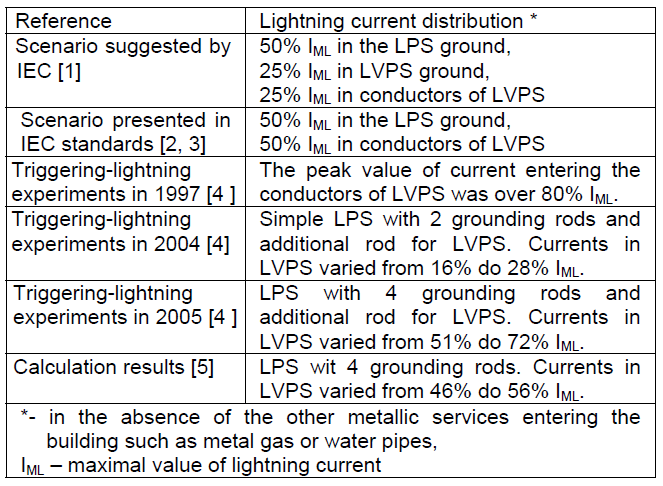
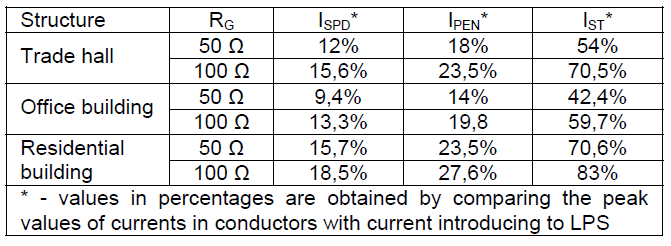
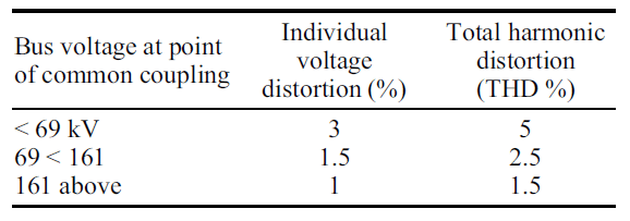
It was characteristic of the different analyses and measurements that these currents were a large part of total lightning current (Table 1).
Table 1. Lightning currents distribution during direct strike to LPS
.
In this paper, the great attention has been paid to develop suitable models for evaluating the lightning current distribution within the conductors of LVPS and especially the stress of individual SPD.
Models description
In paper only the low-voltage side of distribution system has been considered. Analyses were done for the LVPS with one stage protection systems – the arrangements with voltage-switching SPDs type 1 inside the structure. In theoretical consideration the model of SPD was realized on the base of switch with additional resistor, when the switch is closed. The spark-over voltages of SPDs were 1500 V and 2500 V.
Furthermore the impedances, such as inductances and resistances of the SPDs connections also are included. The LVPS was connected to the distribution transformer located outside the structure. The earthing impedance of the transformer is represented by L3 I R3 [6]. The basic of LVPS has been converted into equivalent circuit diagram presented in Fig.1.
Fig.1. Circuit diagram for LPS with switching SPD type 1
In analysis the surge currents 100 kA and 150 kA (peak values) and shape 10/350μs were used for simulation the first lightning strokes.
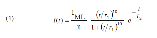
This lightning current was described by typical equation [7]:
.
where: IML = peak values of current (100 kA or 150 kA), η = 0,930, 𝜏1 = 19 μs, 𝜏2 = 485 μs, t -time
Calculations were realized for LPS model of the trade hall with dimensions 48 m x 12 m x 12 m (case A). Down conductors were connected to simple earth electrodes type A with resistance RG = 6,4 Ω (Fig. 2).
Fig.2. Model of LPS and LVPS used in calculation (case A)
Additionally, the calculations were realized for LPS of 2 types of structures and the following conditions were considered:
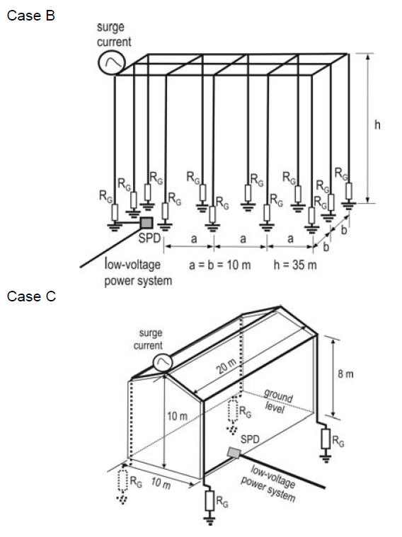
Case B – office building (Fig. 3) • lightning protection level II, • base equal 20 m x 40 m and height h = 20 m, • the mesh side of the air-termination system on the roof was 10 m x 10 m, and the distance between down conductors 10 m, • conductors of LPS with radius 4 mm, • surge currents were injected to the corners of LPS, • earth termination system type A with earth electrode resistance RG = 10 Ω.
Case C – residential building (Fig. 3) • lightning protection level IV, • base 10 m x 20 m and maximal high 10 m, • four down conductors at each edge of the structure, • conductors of LPS with radius 4 mm, • earth termination system type A with earth electrode resistance RG = 21 Ω.
Calculation results
Theoretical calculations of lightning current distribution are based on the simple circuit theory approach. In models, the conductive elements of LPS have been represented with an equivalent π model taking into account resistance and self-inductance, the inductance coupling with another segments and capacitance to the ground.
In the proposed models the influence of current in lightning channel between striking point and cloud were not considered. In calculation The Electromagnetic Transient Program EMTP [8] was used.
Examples of computed currents (case A) that flow to the earthing system of transformer through the PEN and phases conductors are shown in figure 4.
Fig.3. Diagram of lightning protection systems (case B and C)
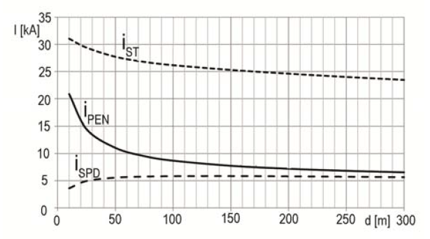
Fig.4. Calculated waveforms for currents in SPD (iSPD), PEN conductor (iPEN) and in earthing system of transformer (iST)
The overall division of lightning current is influenced by many factors. In calculations the following were considered:
• resistance R3 in range from 1 Ω to 20 Ω (Fig. 5 and 7). • distance d between transformer and SPDs from 10 m to 300 m (Fig. 6),
A reduction of the partials lightning currents in SPDs and PEN conductor can be achieved if the LVPS bounding bar is connected to additional grounding rod RAG. In calculations the values of RAG were the same like RG in LPS.
Fig.5. Maximal values of currents with increasing values of transformer grounding system (case A, d = 100 m, w = 2m), a) currents in SPD and in PEN conductors, b) total current in LVPS
Changes in surge current distribution caused by additional grounding rods are presented in Fig. 5.
Fig.6. Maximal values of currents in conductors of LVPS (case A, w = 2m) with increasing distance d between SPD and transformer
Fig.7. Maximal values of currents in conductors of LVPS with increasing values of transformer grounding system (d = 100 m, w = 5 m,, a) office building – case C, b) residential building – case C
In order to comparison the effect of LPS on current distributions in conductors of LVPS calculations were realized with the same conditions in analyzed structures (values of RG, R3 = 5 Ω, distances d = 100 m and w = 5 m). Some results are presented in table 2.
Table 2. Maximal values of currents in conductors of LVPS
.
Conclusions
In this paper the results of numerical calculations of lightning currents in low-voltage power systems supplying different types of buildings during direct strikes to LPS were presented.
The knowledge of these currents may be great importance for an accurate determination of adequate SPD system in low-voltage installations inside the structures, more accurately than it can be done using the procedures suggested by international standards.
Further studies will be performed to correct models of SPD, low-voltage installations and load inside the structures.
REFERENCES
[1] Rakov V. A., Uman M. M., Mata C. T., Rambo k. J., Stapleton M.V., Sutil R.R., Direct Lightning Strike to the Lightning Protective System of a Residential Building: Triggered- Lightning Experiments. Trans. on Power Delivery, vol. 17, No. 2, 2002, p.575-586 [2] IEC 62305-3, Protection against lightning – Part 3: Physical damage to structure and life hazard. [3] EN 61643-11, Surge protective devices connected to low-voltage systems. [4] DeCarlo A., Rakov V. A., Jerauld J.E., Schnetzer G. H., Uman M., Schoene J.: Distribution of Currents in the Lightning Protective System of a Residential Building – Part I : Triggered Lightning Experiments. Trans. on Power Delivery, vol. 23, No. 4, 2008, p.2439-2446. [5] Celli G., Ghiani E., Pilo F. A simulation tool for overvoltages brought inside a building through its grounding system. 26th International Conference on Lightning Protection, Cracow, Poland, 2002, 7b.2 [6] Birkl J., Zahlmann P.: Lightning currents in low-voltage power installation, 29th International Conference on Lightning Protection, Uppsala, Sweden, 2008, p. 10-1-1 – 10-1-25. [7] IEC 62305-1, Protection against lightning – Part 1: General principles. [8] ElectroMagnetic Transients Program (EMTP) Rule Book, http://www.eeug.org
Autor: dr hab. inż. Andrzej W. Sowa, prof. P.B., Politechnika Białostocka, Wydział Elektryczny, 15-351 Białystok, ul. Wiejska 45D, E-mail: Andrzej.sowa@ochrona.net.pl
Source & Publisher Item Identifier: PRZEGLĄD ELEKTROTECHNICZNY (Electrical Review), ISSN 0033-2097, R. 88 NR 9b/2012
Published by Jarosław WIATER, Białystok University of Technology
Abstract. Step voltage situation arise when it is possible for a person to make simultaneous contact with a part of an electrical system which is not live under normal conditions but has become live due to the passage of current for example lightning strike one. The purpose of this paper is to provide knowledge about the levels of step voltages around tree without lightning protective system during direct lightning stroke to it. Step voltage measurement results were presented for maple tree. High voltage surge generator were used as an excitation source (37kA, 8/26μs).
Streszczenie. Różnica potencjałów na powierzchni ziemi determinuje powstanie napięć krokowych. Bezpośrednie wyładowanie piorunowe w drzewo może spowodować ich powstanie. W tym artykule zaprezentowano wyniki pomiarów napięć krokowych, które powstały przy przepływie prądu udarowego przez Klon Zwyczajny. Jako źródło wymuszające wykorzystano wysokonapięciowy generator prądów udarowych – 37kA, 8/26μs. (Napięcia krokowe w pobliżu drzewa przy wymuszeniu w postaci prądu udarowego).
Keywords: step voltage, lightning, measurements, maple tree. Słowa kluczowe: napięcie krokowe, wyładowanie piorunowe, pomiary, klon zwyczajny.
Introduction
The direct lightning strike to tree not equipped with lightning protective system (LPS) can be dangerous for the people standing nearby it. Transient step voltages can arise on the ground surface due to surge current injected into the soil by the earth electrode which it this particular case can be tree trunk and tree roots. There isn’t much information about the life hazard caused by transient electric stress on human being.
As well known ventricular fibrillation is caused when an electrical stimulus of sufficient strength strikes the heart in the vulnerable period. This period which is represented in the electrocardiogram by the T-wave, is characterized by a non-homogeneity or differences in the refractoriness of the heart fibres. Only then can fibrillation be initiated, and it is self sustained by cyclic excitations. Fibrillation of the ventricles (the main pumping chambers) is accompanied by a loss of coordinated muscular contraction and the heart muscle quickly becomes exhausted and, if the condition is not soon corrected, an irreversible standstill of the heart occurs [1, 7].
Measuring situation description
Step voltage level is strictly correlated with tree root system. Situation is similar to grounding system case. Most tree roots do not penetrate very deeply into the soil. Unless the topsoil is bare or unprotected, trees will concentrate most of their absorbing roots in the top 15 to 45 cm of soil, where water, nutrients, and oxygen can be found. Tree root systems cover more area than might be expected – usually extending out in an irregular pattern 2 to 3 times larger than the crown area. However, on a dry weight basis, the “root to shoot” ratio is around 20 to 80%, making the top four to five times heavier than the roots. The type of roots formed initially is specific to a given species with age the initial root form is often modified by the growing environment. Such thing as soil hard-pans, water tables, texture, structure, and degree of compaction all influence the mature root form. There are three basic classes of tree root systems:
a) tap root (for example: hickory, walnut, butternut, white oak, hornbeam), b) heart root (for example: red oak, honey locust, basswood, sycamore, pines), c) flat root presented on figure 1 (for example: birch, fir, spruce, sugar maple, cottonwood, silver maple, hackberry).
Fig. 1. Maple flat tree root system and transient step voltage measurement method.
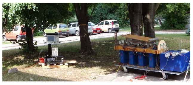
In small park for the measurements purpose maple tree were selected. Maple tree should create worst case with respect to step voltage level because flat root system. On figure 2 were presented photo taken during measurements.
Fig. 2. Step voltage measurements in progress
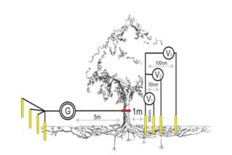
The step potential is defined as the potential difference between a person’s outstretched feet, normally 1 meter apart – figure 1, without the person touching any earthed structure [4] – human worst.
For the purpose of circuit analysis, the human foot is usually represented as a conducting metallic disc and the contact resistance of shoes, socks, etc., is neglected [4]. Traditionally, the metallic disc representing the foot is taken as a circular plate with a radius of 0,08 m. A value of 1000Ω were used as a resistance of a human body from one foot to the other foot [4]. During the measurements voltage electrodes dug on 0,08m depth represents human foot.
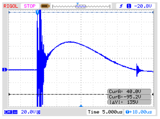
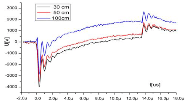
Arrangement during the step voltage measurements presents figure 3. High voltage generator were connected to the maple tree by copper ring. Ring were installed on 1,3m height from ground level. Current loop were closed by four additional current electrodes putted on square traverse. High voltage generator produced 8,4/26,4μs current surge with Imax=37kA [8]. Current waveform presents figure 4. Generated surge current forces step voltages nearby the tree.
Fig. 3. Arrangement of step voltage measurements – front view
Fig. 4. High voltage surge generator output current
All recorded waveforms were presented on figure 5 and 6 for different time window. Maximal value depends on time moment. In first microseconds step voltage have got negative polarization and reaches 4kV for smallest foot distance. This voltage jump is strictly correlated with high voltage generator. At time t=0μs internal capacitors were connected to output by triggering mechanism. This forces high voltage level at nearby t=0μs time. It seems possible that voltage level during real lightning strike can reach millions volts. This phenomenon will be analyzed in future time [9-14].
At fourteen microsecond step voltage have got positive polarization and reaches 2,8kV for 100cm foot distance.
Fig. 5. Step voltage nearby tree – view for t∊<0;100>μs
Fig. 6. Step voltage nearby tree – view for t∊<0;18>μs
Conclusion
In order to ensure the safety of people at a open area, it is necessary to ensure that step potentials in and around the yard during lightning conditions are kept below set limits. These maximum permitted step potentials are addressed within various national and international electrical standards. The results of measurements of lightning transient step voltage distributions in an around a tree in case of direct lightning stroke to it were presented above. Observed step voltage exceed two times safe level according IEEE Std 80 2002 [3]. Main factor which determine step voltage distributions were different tree roots classes. Trees such as birch, fir, spruce, maple, cottonwood, silver maple, hackberry and they root system provides highest step voltage levels.
This work was co-funded by the European Union under the European Social Fund.
REFERENCES
[1] Biegelmeier G, Lee WR.: “New considerations on the threshold of ventricular fibrillation.” IEEE Proceedings Vol 127, No 2, Pt A, March 1980. [2] BS 7354 – 1990: Code of practice for Design of high-voltage open-terminal stations. [3] IEEE Std 80-2002: IEEE Guide for Safety in AC Substation. [4] Electricity Association Technical Specification 41-24: Guidelines for the Design, Installation, Testing and Maintenance of Main Earthing Systems in Substations. [5] PN-E-05115:2002. Instalacje elektroenergetyczne prądu przemiennego o napięciu wyższym niż 1kV. PKN, Warszawa 2002. [6] W.Simpson, A. TenWolde “Physical Properties and Moisture Relations of Wood”. http://www.fs.fed.us/. [7] http://ballengearry.com.au/papers/Step_and_Touch_Voltage_ update_for_2004_090804.pdf [8] Augustyniak L.: Surge voltage portable generator generating 1.2/50 mu s test waveshape of peak value up to 4 kV. Przeglad Elektotechniczny. V: 83, Issue: 9, pp. 37-38, 2007. [9] Markowska R.: Analysis of Lightning Electromagnetic Exposures in Building Electrical Installation with SPD. Przeglad Elektrotechniczny, V:86, Issue: 3, pp. 48-50, 2010. [10] Sowa A.: Coordination the solutions of lightning protection system with electromagnetic compatibility requirements. Przeglad Elektrotechniczny, V: 85, I:9, pp. 332-339, 2009. [11] Wiater J.: Lightning hazard minimization of the HV substation signal ports. Przeglad Elektrotechniczny, Volume: 86, Issue: 3, pp. 172-175, 2010. [12] Wiater J.: Analyzer and lightning voltage surge logger for data transmission lines. Przeglad Elektrotechniczny, Volume: 86, Issue: 11B, pp. 97-98, 2010. [13] Wiater J.: Remote earth localization for lightning surge condition on the high voltage substation. Przeglad Elektrotechniczny, Volume: 86, Issue: 3, pp. 96-97, 2010. [14] Wiater J.: Influence of Different Lightning Source Models on Current Distribution in the HV Substation. Przeglad Elektrotechniczny, Volume: 86, Issue: 3, pp. 94-95, 2010.
Authors: dr inż. Jarosław Wiater, Bialystok University of Technology, Department of Telecommunications and Electronic Equipment, ul. Wiejska 45d, 15-351 Białystok, Poland. E-mail: jaroslawwiater@we.pb.edu.pl
Source & Publisher Item Identifier: PRZEGLĄD ELEKTROTECHNICZNY (Electrical Review), ISSN 0033-2097, R. 88 NR 9b/2012
Published by Wiesław BROCIEK1, Robert WILANOWICZ2, Warsaw University of Technology (1) , Radom University of Technology (2)
Abstract. The paper presents a circuit model of three phase arc arrangement, taking into account the nonlinearity of the arc appearing In the particular phases as well as the windings vector groups of a furnace transformer. This model was designed on the ground of parameters, resulting from a voltage current characteristic of the arc. At modeling of changes of parameters of an arc we applied the random values of resistance. The values of higher harmonics of current and voltage for each considered case have been evaluated by using the simulation program MicroCap – 8. In the paper we have included the exemplary results of numerical calculations.
Streszczenie W artykule przedstawiono model obwodowy trójfazowego urządzenia łukowego z uwzględnieniem nieliniowości łuku w poszczególnych fazach oraz grupy połączeń transformatora piecowego. Model ten opracowano na podstawie parametrów wynikających z nieliniowej charakterystyki napięciowo – prądowej łuku. Do symulacji zmian parametrów łuku elektrycznego wykorzystano generator zmienny losowo. Wszystkie obliczenia zostały przeprowadzone w programie MicroCap – 8. Obliczono wartości wyższych harmonicznych prądu i napięcia w odbiorniku oraz po stronie pierwotnej i wtórnej transformatora piecowego. Zamieszczono przykładowe rezultaty obliczeń numerycznych. (Zniekształcenia napięcia i prądu w układzie zasilania pieca łukowego)
Keywords: nonlinear load of random parameters, higher harmonics of current and voltage. Słowa kluczowe: odbiornik nieliniowy o parametrach zmiennych losowo, wyższe harmoniczne prądu i napięcia
Introduction
One of the crucial parameters describing the quality of the electrical energy are these describing the distortion of the voltage an current from the ideal sinusoid. They may be measured by the higher harmonics, i.e. contents of higher harmonics and their values. Because of consequences for power system followed by the higher harmonics the obligatory standards define the upper limits of distortion, acceptable in the system. Determination of the distortion degree caused by the applied electrical equipment is the fundamental task in the qualification of the correct performance of this equipment.
The article present results of simulation tests concerning the cooperation of the nonlinear load (AC – arc furnace) with the power system are presented. The values of higher voltage and current harmonics and total harmonic distortion on the primary and secondary sides of arc furnace transformer 30/0.75 kV for each considered case have been evaluated by the experiments performed by using the simulation program MicroCap-8.
System description
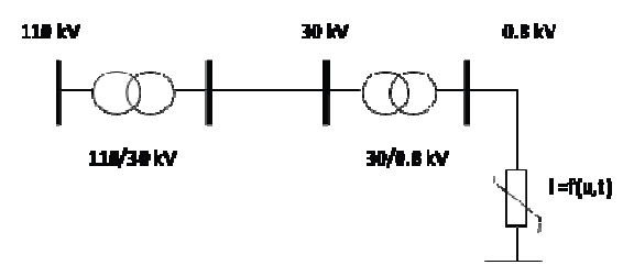
Figure 1 presents the general scheme of power system supplying the nonlinear load i = f(u). Fig. 1 presents the simplified power supply diagram of electric steel works with arc-arrangements. A three phase arc arrangement consists of: an arc furnace, strong-current circuit and furnace transformer. Accurate description of the effect which could make possible to create a precise model of the arc arrangement. is rendered difficult. However, one should carry out investigations in this course in orders. to create a model of UHP arrangement which would reflect real operating conditioners.
Fig.1. The general structure of the simulated system
The model presented in Fig. 1 is composed of the following elements: supplying point 110kV of short-circuit power Szw= 500MVA, the main supplying point (PCC) 30kV of short circuit power Szw=200MVA, transformer 30/0.75kV, S=75MVA and nonlinear load i=f(u,t ) – arc furnace.
The parameters (RS, LS) of the model representing the supplying systems on the level 30kV have been determined using following formulas (for f=50 Hz) [3].
.
Fig.2.The circuit model of the analysed system at nonlinear load in 3 phases
To ensure the continuity of arc current each electrode is controlled by independent controller. As a result the electrodes currently move depending on iron charge resistance, charge shape and phase of technology process. Currents of three-phase line are random functions. Fig. 2 shows the system with three controlled sources modelling current-voltage arc characteristics and resistances modelling the state of arc stability of each electrode. It means that system to be analyzed is nonlinear and its parameters are random [2,3,4].
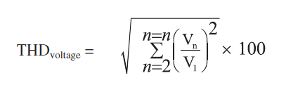
To the largest and most energy consuming nonlinear high power receivers belong siderurgical arc arrangements provided with transformers amounted to power of tens MVA. The characteristic feature for the coding of charge period consists in very rough and irregular mutability of power consumption by the furnace caused by nonlinear variations of the arc resistance as well as variations of the plasma physicochemical properties in the arc’s column. The arc furnace becomes then a nonlinear asymmetric receiver, and at low level of short-circuit power it gives occasion to interferences in the power supply network, thus making worse quality of electric power supplied from the heavy current system to other consumers. Such interferences include: fluctuations and asymmetry of voltage as well as deformation of voltage curve. As the electric arc is an element of nonlinear voltage-current characteristic, therefore, the furnace draws out of the network; a considerably deformed current and becomes a source of higher currents’ harmonics. Investigation of influence of siderurgical arc arrangements on the electric power system wants establishment of higher harmonics current distribution in this system. This makes it possible to determine voltage drops of higher harmonics as well as those harmonics of voltage in any node of the system. One of the determination procedures of voltage distortion degree consists in determination of the voltage distortion factor THDV determined by the following relation [1,3]
.
The admissible values of voltage distortion for 30kV are [4]
.
The admissible values of voltage distortion for 110kV are [4]
.
The represented model was designed on the ground of parameters resulting from the empirical determination method of the arc voltage-current characteristic [1,3].
The furnace transformer 30/0.75 kV of power S=75 MVA has 12 degrees of voltage control. Low secondary voltage of this transformer is its characteristic feature. The most advantageous scheme of connections of a two-winding furnace transformer is:
the primary winding with delta connection changed over voltagelesely into a star connected winding,
the secondary winding should be always with delta connection.
Connection of the furnace transformer secondary terminals into triangle shows the following superiority in comparison with connection into star:
the short-circuit current between electrodes is distributed into two phases of the transformer,
connection of secondary terminals into triangle makes it possible to realize a so-called three-phase bifilar circuit.
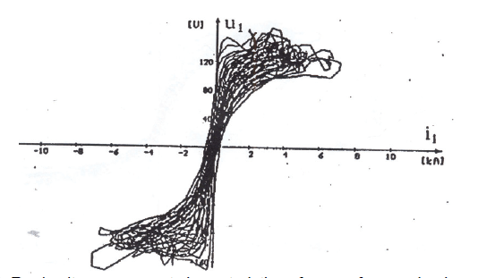
Fig.3. Voltage – current characteristics of an arc furnace in phase A
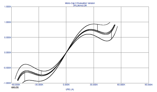
Fig. 3 presents the exemplary voltage – current characteristics of an arc in phase A. In numerical calculations we have considered the voltage-current characteristics of the real AC arc furnace. They are presented in Fig. 4.
Fig.4. Real voltage – current characteristics of an arc furnace in phase A
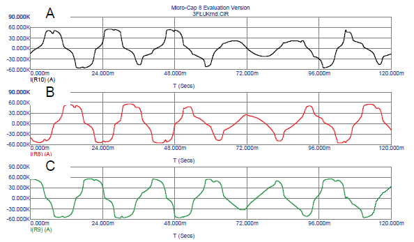
Fig.5. Instantaneous values of current In electrodes A, B, C
Fig.6. Instantaneous values of a) currents on the primary side of transformer, b) the voltage on the secondary side of transformer.
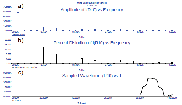
Fig.7. Deformation of currents in electrode A, a) rms values of harmonics, b) the percent distortion versus frequency, c) the waveform of the current
Fig.8. Deformation of currents in phase A, a) rms values of harmonics, b) the percent distortion versus frequency, c) the waveform of the current .
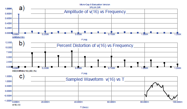
Fig.9. Deformation of voltages in electrode A, a) rms values of harmonics, b) the percent distortion versus frequency, c) the waveform of the voltages
Figures 5 and 6 presents instantaneous values of currents on the primary side of transformer, the voltage on the secondary side of transformer and current of the electrodes. Figures from 7 to 10 presents the distorted currents & voltages in the system of Fig. 3. Tables 1 and 2 presents the values of currents & voltages harmonics in the circuit of Fig. 3 at nonsymmetrical load.
Fig.10. Deformation of voltages in phase A, a) rms values of harmonics, b) the percent distortion versus frequency, c) the waveform of the voltages
As a results of simulation we hale got the currents and voltages of the values very close to that in real operation of the system. After determination of the currents and voltages we can easily the other parameters of the system including the rms values of harmonics, as well THD coefficient being the basic measures of the quality of electrical energy.
Table 1. The values of the current harmonics in the circuit of Fig. 3 at nonsymmetrical load.
.
Table 2. The values of the voltages harmonics in the circuit of Fig. 3 at nonsymmetrical load.
.
Conclusions
For simulation of the changes of parameters of the electric arc we have used the random number generator built In MicroCap program.
The performed experiments allow to determine the propagation of the higher harmonics of the voltage and current generated by the nonlinear load in the power system. The model can by easily extended to the other nonlinear loads, for example the arc furnace supplied from the real system.
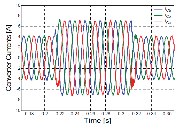
The comparison of the shapes of the currents in the 3 phase real system and in our model has confirmed the accuracy of the proposed approach. The results of simulation and measurements allow to assess the level of generated higher harmonics by nonlinear loads and influence of these harmonics on power system.
The modeling and simulation AC arc furnace, is a handy and recommended tool for the analysis of the power system cooperating with the nonlinear load.
This research activity was financed by the National Science Centre.
REFERENCES
[1] Brociek W., Wilanowicz R. Electric power quality parameters in transformer stations supplying nonlinear load, Przegląd Elektrotechniczny, 11/2003, pp.861 – 864. [2] Ozgun O.Abur A.Flicker study using a novel arc furnace model, IEEE Transactions on power delivery, vol 17 no.4.10, 2002 [3] Brociek W., Wilanowicz R., Siwek K. Determination of the electric power in transformer station supplying nonlinear load: experimental and numerical study, V CPEE, Jazłowiec 2003, pp.141-144. [4] Wang Y.F., Jiang J.G. A novel chaotic model of electric arc furnace for power quality studies, Proc.of Int. Conf. on Electrical Machines and Systems 2007, Oct. 8-11, Seoul, Korea.
Authors: dr inż. Wiesław Brociek, Warsaw University of Technology, Institute of Theory of Electrical Engineering, Measurement and Information Systems, E-mail: brociek@iem.pw.edu.pl, dr inż. Robert Wilanowicz, Radom University of Technology.
Source & Publisher Item Identifier: PRZEGLĄD ELEKTROTECHNICZNY (Electrical Review), ISSN 0033-2097, R. 87 NR 7/2011
Published by Liu Liqun, Liu Chunxia, Taiyuan University of Science & Technology
Abstract. This paper gives the techno-economic analysis of a wind-PV-diesel system with storage battery backup for an off-grid power station specially located in Dongwangsha, studying data from a particular site in littoral China. The simulation and optimization results indicated the most optimized sizing of hybrid system. Moreover, the sensitivity analysis is discussed at a diesel price of 2$/L and annual average wind speed of 4.41 m/s and interest rate of 6%. The proposed hybrid system is more cost effective and environmental friendly than the diesel only system.
Streszczenie. W artykule przestawiono techniczno-ekonomiczną analizę systemu energetycznego składającego się z urządzeń wiatrowych, fotowoltaicznych i silnikiem Diesla oraz baterii magazynującej na przykładzie sieci w miejscowości Dongwagsha w Chinach. Rezultaty symulacji i optymalizacji pokazały, że system hybrydowy jest znacznie korzystniejszy niż tylko oparty na silniku Diesla. (Techniczno-ekonomiczna analiza systemu hybrydowego z wykorzystaniem źródeł odnawialnych – na przykładzie Chin)
Keywords: Renewable energy; Techno-economic analysis; Hybrid power supply system. Słowa kluczowe: energia odnawialna, analiza ekonomiczna, hybrydowy system energetyczny
Introduction
It is well known that China is the largest developing country and the second largest energy consumption country in the world. The total consumption amount of coal and oil are more than 2.74 and 0.36 billion tons in 2008, respectively, and natural gas is about 80.7 billion m3 [1]. Abundant energy consumption brought a lot of pollutants and a large amount of emissions. For example, the SO2 emission from 2000 in China is more than 20 million tons, which ranks the first in the world [2]. The CO2 emission is more than 4.5 billion tons, which ranks the second in the world [3]. The total pollution loss accounts for 10% of Chinese Gross Domestic Product [4]. Chinese primary energy supply structure is very inappropriate [5]. Chinese central government and local governments have waked up to the problem to realize the sustainable development of country in future. Renewable Energy Law has been established in February 28, 2005. The development and application of renewable energy has been regarded in order to improve the inappropriate energy structure. The renewable sources in China are abundant, such as wind, solar, and biomass energy, etc. For example, the total amount of wind power in China is more than 3.2 billion kilowatts at 10 meter height, and the amount which can be effectively utilized is about one billion kilowatts. As a conclusion, the prospect of renewable energy in China is beautiful in foresee future.
The conventional power grid in China can not supply the total end consumers with enough power. In this period of time, millions of off-grid consumers have to use the diesel generator in order to receive the supply of power. Moreover, some industry equipments located in remote areas which apart from the power grid, such as communication base station, island power system, and radar station, and so on. The generating system uses the renewable sources can afford steady electricity supply. For example, some standalone PV power stations have been established in remote areas to improve the power quality of off -grid consumer which have enhanced the standard of living of ordinary people. However, a common drawback is existed in the stand-alone wind energy and solar energy generating power system, and the output electric power is unpredictable which change with the changing of weather, such as insolation, temp, and wind speed, etc. Fortunately, the hybrid wind-solar system can partially overcome the problems which integrate multi-fold resources in a proper combination, and the output quality of power is improved. But the price of wind power generator and PV is costly at present and the initial capital of hybrid only wind-solar system is big. The expensive levelized cost of energy (COE) can not be accepted by the ordinary user. The conventional diesel only power system consumes a lot of diesel and discharge a mass of greenhouse gases. Fossil resource came in increasing price, and the hybrid generating system is suggested to offer steady and reliable and cheap power supply for the off-grid user or the industry equipment as compare with the diesel only generating system. Certainly, the techno-economic analysis of hybrid system is necessary to minimize the initial capital, COE, operating & maintain cost (O&M), net present cost (NPC), diesel consumption and unmet electric rate at suffice for consumer’ need.
Many literatures have analyzed the feasibility of renewable resource generating system by using HOMER or Hybrid2 or RETscreen [6-14]. Unfortunately, the renewable power supply system in China did not consider the optimal analysis of components of renewable resources power system at present. The article presents the feasibility analyses of renewable power station to optimal configure and reduce the initial capital and NPC. In order to arouse the regard of designer, an established power station is used to compare with the proposed optimal system. In this context, the present study carries out a techno-economic analysis by using HOMER software of the USA National renewable Energy Laboratory (NREL) and the data of National Aeronautics and Space Administration (NASA) to optimize configure of a hybrid wind-PV-diesel system with storage battery backup for an off-grid power station which located in Dongwangsha, Chongming islands [15-16].
Site and Meteorological data and Electrical load
Dongwangsha located in Chongming island of Shanghai where apart from the national electrical grid. The village gets power through diesel generating power plant in the past. The diesel only system is difficult to ensure the continuous electricity supply during breakdown and scheduled shutdown of diesel units. A hybrid wind-PV-battery power station has been established in the site that is capable of meeting the load. The geographical coordinates of the data established project site were 31o31′ N latitude, 121o57′ E longitude and 1 meter altitude above mean sea level. The existing meteorological data of wind speeds are measured at 40 meters height according to an established wind speed weather station located in project site, but without accurate data of solar insolation clearness Index, earth skin temperature, relative humidity, and wind speed at 10 meters altitude above the surface of the earth.
The meteorology data from NASA is used to the proposed hybrid system. The monthly average daily total global solar radiation (GSR) ( kW / m2 / d ) and clearness index are shown in Fig.1 (a), and the data is gained via internet by using HOMER based on the latitude and longitude. The scaled annual average value of GSR is 3.95kWh/m2 / d . The highest values of GSR are gained during the months of May to August with a maximum of 5.559kWh/m2 / d . The lowest values are gained during the months of December to January with a minimum of 2.183kWh /m2 / d .According to solar radiation, Fig.1 (b) shows that the hourly available PV power output throughout the year.
Fig.1. Meteorological data of solar insolation and available power output at the site
The monthly average daily wind speed (m/s ) at the 10 meter above the surface of the earth was collected from NASA as shown in Fig.2 (a), and the scaled annual average value of wind speed is 4.41m/s. The highest values of wind speed are observed during the months of January to February with a maximum of 4.91m/s . The lowest values are observed during the months of May with a minimum of 3.97m/s. The hourly available power output throughout the year according to wind speed is shown in Fig.2 (b). Moreover, the annual average wind speed can not same, and the considered wind speed in this paper are 4, 4.41, and 5m/s .
Fig.2. Meteorological data and available wind speed at the site
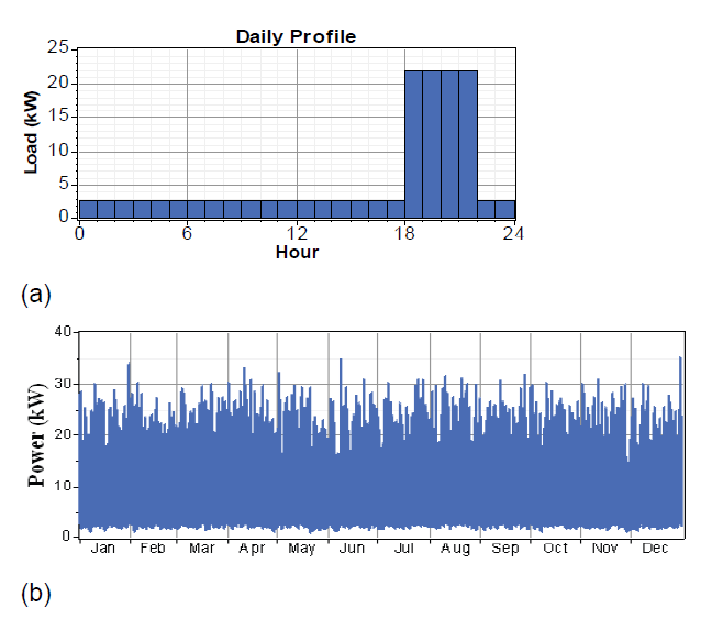
Fig.3. Variation of Load demands of proposed project.
The hybrid wind-solar only system with one wind turbine of rated power 5kW and PV with rated power 34.3 kW and 990 batteries with rated capacities 100Ah and rated voltage 2V have been established in the Dongwangsha. The initial capital is about 251,397$. The typical hourly electrical consumption data used in this project was measured and described in literature [17]. The average value per day of load was 139kWh, and the maximum hourly power of the load was 35kW, and the daily load factor varied from 0.074 to 0.629. Fig.3 (a) shows the typical hourly load demand. The highest values of electric consumption appeared between 18:00 hours and 22:00 hours with a maximum power of 22 kW , and the lowest value of load demand appeared between 22:00 to 16:00 of the following day with a minimum power of 2.6kW , and the rated voltage of load is 220V. As shown in Fig.3 (b), the hourly available electric consumption throughout the year is varied with season changing.
Hybrid wind-PV-diesel-battery power station
A hybrid wind-PV-diesel-battery power station is used to discuss the possible optimal configure of power station in Dongwangsha, and the proposed autonomous hybrid system consists of one diesel generator, some PV arrays, some storage batteries, some wind power generators, and a power converter. The hybrid power with battery backup is used to maintain regular supply during the conspicuous bad weather and breakdown and scheduled shutdown of diesel unit. The hybrid power system optimization software HOMER developed by NREL has been used in this proposed power station, which is a computer model to assist in the design of micro power systems and to facilitate the comparison of power generating technologies across a wide range of applications. The physical behavior and lifecycle cost and total cost of installing and operating the system over its life span of a project is described. HOMER allows the modeller to compare with many different design options based on their technical and economic merits. It also assists in understanding and quantifying the effects of uncertainty or changes in the sensitivities [16].
Solar PV modules are connected in series and parallel string in order to produce enough electric power according to the voltage and current demand of load. The initial capital and the replacement cost of PV are 4400$ and 4400$ per kilowatt ($/kW) in China, respectively. The PV sizes are considered to be 0, 10, 15, 20 and 25 kW. Operation and maintenance cost of PV array is 20$/kW per year. PV array were considered as fixed and the slope degree is 31.5. Working lifetime of PV panels are taken as 20 years and don’t consider the tracking system. The effect of temp for PV output power is considered in the article. Temp coefficient of power is -0.5%/oC , and nominal operating cell temp is 47oC and output power efficiency is 13% at standard test conditions.
The horizontal-axes wind turbine series of Guangdong Shangneng wind power equipment ltd. (GSWPEI) are considered for the proposed power station design. SN-3000WL type wind electric generator is considered for this project via compare with the cost of per watt of other types. The initial capital and the replacement cost of wind turbine are 2100$ and 2000$ per kilowatt, respectively. Five different wind turbines quantities (0, 20, 24, 28 and 32) are taken in the hybrid system. Operation and maintenance cost of wind turbine is considered to be 20$ per year, while the working lifetime of wind turbines and the hub height are taken as 15 years and 15 meters, respectively. The output power of SN-3000WL type wind electric generator during various wind speed can be seen from literature [18].
A battery band is used as a back up system to maintain the electric consumption at bad weather. SN150-12 type battery is considered for the proposed project which is produced by GSWPEI, and the nominal capacity and nominal voltage of each battery are 150 Ah and 12V, respectively. Round trip efficiency and minimum state of charge are taken as 85% and 30%, respectively. The float life, maximum charge rate and maximum charge current are 10 years, 1A/Ah and 18A, respectively. The lifetime throughput and suggested value are 1075 and 2343 kWh.
The initial capital and the replacement cost each battery is considered to be 110$ and 100$, respectively. Operation and maintenance cost is 2$ per year. The battery quantities are considered to be 0, 48, 120, 192, 264, and 336. The initial capital and the replacement cost of diesel generator is taken as 220$/kW and 200$/kW, respectively. The diesel generator sizes are considered to be 0, 15, 20, 30 and 35 kW. Operation and maintenance cost is 0.04$/hr per year. Operating lifetime hours are 15000 hours and minimum load rate is 30%. Furthermore, the carbon monoxide and unburned hydrocarbons and particulate matter and nitrogen oxides of fuel are 6.5, 0.72, and 0.49, and 58 gram per liter (g/L), respectively. And proportion of fuel sulfur converted is 2.2. The current diesel price per liter in China is about 1$. The price of diesel is used for sensitivity analysis and five discrete values (0.5, 0.8, 1, 1.2, and 2 $/L) were considered.
The power converter is needed to maintain power flow between the AC and DC components. The initial capital and the replacement cost of power converter is about 195$ and 195$ per kilowatt, respectively. Six different sizes of power converter (0, 25, 30, 35, 40 and 45 kW) are taken in the model. Operation and maintenance cost is taken as 0$ per year. The lifetime is 15 years. Inverter and the rectifier efficiency is 90% and 85%, respectively.
The annual real interest rate is taken as 6%, and the interest rates are considered to be 4%, 6%, and 8%. The project lifetime is 25 years. Dispatch strategy uses cycle charging. Apply set point state of charge is 80%. Operating reserve includes the percent of load and percent of renewable output, and the hourly load as percent of load is 10%, and solar power output and wind power output is 25% and 50%, respectively.
Optimal results and discussion
According to the above input, there are 202,500 possible system configurations which comprised of 45 sensitivities and 4500 simulations for each sensitivity run. Table.1 displays the values of each optimization variable to simulate all possible system configurations. HP pavilion ze2000 notebook PC, AMD Sempron 2800+ CPU, with 1.59 GHz speed, 768 MB took 1 hour, 31 minutes and 12 second to calculate the possible configurations.
Table.1. Probable of system configurations
Source: Authors’ new contribution to this paper
Table.2 summarizes the optimization results for a wind speed value of 4.41m/s (annual average wind speed at the site), interest rate of 6%, and the diesel price in China, which currently equals 1$/L. The suggested optimal hybrid wind-diesel-battery (WDB) power station consists of 32 wind power turbine with rated power of 3kW, 15kW diesel generator, 336 batteries, and 40 kW sized power converter. The proposed hybrid system was found to have an initial capital of 115,260$ with an annual operating cost of 7,002$, total NPC of 204,775$, COE of 0.316$/kWh, renewable energy fraction of 0.955, the diesel consumption of 1,314 L, and working hours of 282 hours. The suggested system of HOMER decreases initial capital of 136,137$ (251,397$-115,260$) as compare with the established hybrid wind-PV-battery system, and the NPC of suggested system of HOMER is less than the initial capital of hybrid system in literature [17]. The only hybrid wind-PV-battery system is considered for the power station, which can be seen in the third row from Table.2. The system with 10 kW PV, 32 wind turbine with rated power of 3kW, 336 batteries, and 35 kW converter is suggested. The hybrid renewable energy only system increases an initial capital of 39,725$, total NPC of 25,766$, and the COE of 0.039 $/kWh while the operating cost decreases 1,091$ per year to compare with the suggested hybrid WDB system. The renewable fraction is 1. The suggested hybrid renewable energy only system of HOMER decreases an initial capital of 96,412$ (251,397$-154,985$) as compare with the established hybrid wind-PV-battery system in literature [17], and the NPC of suggested system of HOMER is less than the initial capital of hybrid system. The diesel only generating system was found in nine row of Fig.4, which consists of a diesel generator with rated power 35 kW. Which increases an operating cost of 60,796$ per year ($/yr), total NPC of 669,615$, and the COE of 1.032 $/kWh while the initial capital decreases 107,560$ as compare with the suggested hybrid wind-diesel-battery system. The renewable fraction is 0. The diesel consumption increases 50,343L, and the operating hours increases 8478 hours (hrs).
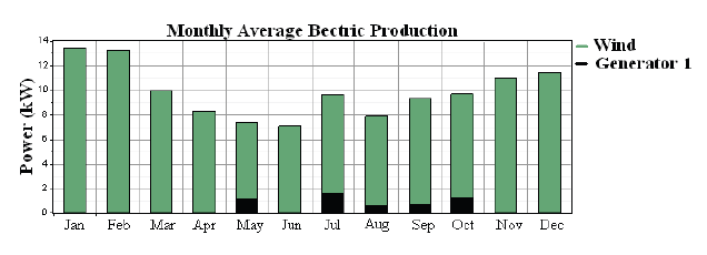
The cash flow summary details of different components for the suggested hybrid WDB system can be seen from Table.3, such as total NPC, initial capital, replacement and operation, fuel and salvage. The suggested hybrid system was able to meet the power requirement of load with 95% wind power and 5% diesel generator power. The AC primary load consumption is 50,709 kWh per year (kWh/yr) and the excess electricity quantity is 23,455 kWh/yr which account for 27.2% of total power production, and unmet electric load quantity is 25.7 kWh/yr which account for 0.1% of total power production, and the capacity shortage is 32.8 kWh/yr which account for 0.1% of total power production. The monthly average electric production is shown in Fig.4. The wind power can meet the power demand during the months of January to April and June and November to December. The diesel generator is operated in May and July and August and September and October to meet the unmet electric load demand.
Table.2. Probable optimal configurations of system
Source: Authors’ new contribution to this paper
Table.3. Cost summary of component
Source: Authors’ new contribution to this paper.
Fig.4. Monthly average electric production of suggested system
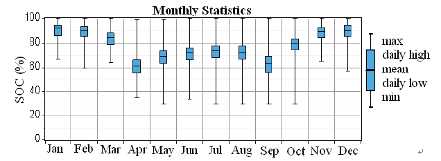
Fig.5. Charge state and monthly storage operating capacity.
The monthly storage operating capacity (SOC) of batteries is shown in Fig.5. The nominal capacity and usable nominal capacity and lifetime throughput are 605 and 423 and 361,200 kWh, respectively. And the autonomy is 73.1 hours (hrs). The battery wear cost and average energy cost are 0.101 and 0.010 $/kWh, respectively. The input energy and output energy and storage depletion and losses and annual throughput are 43,005 and 36,874 and 133 and 5,998 and 39,996 kWh/yr, respectively. The expected life of batteries is 9.03 years. The running characteristic of converter is shown in Table.4. The suggested hybrid wind-diesel-battery power system with 95% wind power could avoid addition of greenhouse gases emissions, such as carbon dioxide, carbon monoxide, unburned hydrocarbons, nitrogen oxides, sulfur dioxide, and particulate matter. The emissions of proposed hybrid system decrease the carbon dioxide of 132,530 (136,031-3,461) kilogram (kg), the carbon monoxide of 327.46 (336-8.54) kg, unburned hydrocarbons of 36.254 (37.2-0.946) kg, particulate matter of 24.656 (25.3-0.644) kg, sulfur dioxide of 266.05 (273-6.95) kg, and nitrogen oxides of 2919.8 (2,996-76.2) kg as compare with the diesel only generating system.
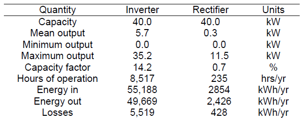
Table.4. Characteristic of converter
Source: Authors’ new contribution to this paper.
Table.5. Probable sensitivity variables
Source: Authors’ new contribution to this paper.
Fig.6. Effect of sensitivities in NPC.
As mention above, there are 45 sensitivity variables which are presented in Table.5. The sensitivity variables will range with the changing of external circumstance, such as meteorological and economical domain. The changing of diesel prices and average values of annual wind speed and different annual real interest rates are considered in this section, which affects the NPC and COE and O&M. For example, the effects of sensitivity variables for NPC are shown in Fig.6. The NPC will increase with the increasing of diesel price and decreasing of annual average wind speed and interest rate. The NPC will decrease with the decreasing of diesel price and increasing of annual average wind speed and interest rate. And the changing of annual average wind speed has the biggest effect for total NPC.
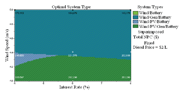
Fig.7. Sensitivity analysis for possible optimal configure.
Fig.7 exhibits the sensitivity analysis results in terms of interest rate and annual average wind speeds for maximum annual capacity shortage of 0%. There are three values for the interest rate and three values for the annual average wind speed were specified. The axes of the graph correspond to these two sensitivity variables. The diamonds in the Figure indicate these sensitivity cases, and the colour of each diamond indicates the optimal system type for that sensitivity case [16]. At the range of annual average wind speed from 4.2 to 4.4 m/s and the interest rate less than 5.5% and the fixed diesel price of 2 $/L, for example, the optimal system type was hybrid wind-PV–battery system. At the annual average wind speed more than 4.4 m/s, the optimal system type was hybrid wind-diesel-battery system. As a conclusion, the design of optimal system must consider the meteorological data of site and external economical condition.
Conclusion
In this article, a hybrid system comprising of wind turbines, PV modules, diesel generator, and storage batteries, is discussed to explore the possibility of utilizing power of the wind and solar to reduce the dependence on fossil fuel for power generation to meet the electric requirement of Dongwangsha located in the seaside of the Chongming islands, Shanghai. The most economical power system consists of 32 wind power turbines with rated power of 3kW, 15kW diesel generator, 336 batteries, and 40kW sized power converter at annual average wind speed of 4.41m/s and diesel price of 1 $/L and interest rate of 6%. The initial capital and total NPC is 115,260$ and 204,775$, respectively. The operating cost is 7,002$ per year and COE is 0.316$/kWh and renewable energy fraction is 0.955 and the diesel consumption is 1,314 L and working hours is 282 hrs. When the power station uses the hybrid renewable energy only system, the economical power system consist of 10kW PV, 32 wind power turbines with rated power of 3kW, 336 batteries, and 35 kW converter. The initial capital and total NPC is 154,985$ and 230,541$, respectively. The operating cost is 5911$ per year and COE is 0.355$/kWh and renewable energy fraction is 1. These suggested systems are more environmental friendly than the conventional diesel only system and the greenhouse gases emission is less than the diesel only system. As a conclusion, the techno-economic analysis is very important to select the optimal configure of hybrid power system.
Acknowledgments: this work was supported by the Program for the Industrialization of the High and New Technology of Shanxi province (NO: 2010016), Youth Science Foundation of Shanxi province (NO: 2011021014-2).
REFERENCES
[1] National Bureau of Statistics of China, 2008. Statistics report of country economy and society development in 2009. http://www.stats.gov.cn/tjgb/ndtjgb/qgndtjgb/t20090226_402540710.htm . [2] CCTV, Strongly promote the development of pollution reduction in transition, 2009. http://hd.cctv.com/20090706/107332.shtml. [3] CCTV, A reporter asked the Ministry of Foreign Affairs denied that China’s carbon dioxide emissions ranks the first, 2007. http://news.cctv.com/china/20070621/108885.shtml . [4] CCTV, The Great Divide of environmental protection: the loss due to pollution in China each year 10% of GDP, 2007. http://finance.cctv.com/20070319/100794.shtml. [5] Chinese Development and Innovation Committee (CDIC), 2008. http://finance.sina.com.cn/roll/20080409/02202131646.shtml. [6] Celik, A.N., The system performance of autonomous photovoltaic-wind hybrid energy systems using synthetically generated weather data, Renewable Energy, 27(2002), No. 1, 107-121. [7] Diaf S., Diaf D., and Belhamel M., et al, A methodology for optimal sizing of autonomous hybrid PV/wind system, Energy Policy, 35(2007), no. 11, 5708-5718. [8] Iqbal M.T., Pre-feasibility study of a wind-diesel system for St. Brendan’s, Newfoundland, Wind Engineering, 27(2003), no.1, 39-51. [9] Khan M.J., Iqbal M.T., Pre-feasibility study of stand-alone hybrid energy systems for applications in Newfoundland, Renewable Energy, 30(2005), no. 6, 835-854. [10] Mills A., Al-Hallaj S., Simulation of hydrogen-based hybrid systems using Hybrid2, International Journal of Hydrogen Energy, 29(2004), no. 10, 991-999. [11] Thompson S., Duggirala B., The feasibility of renewable energies at an off-grid community in Canada, Renewable and Sustainable Energy Reviews, 13(2009), no.9, 2740-2745. [12] Tina G., Gagliano S., and Raiti S., Hybrid solar/wind power system probabilistic modelling for long-term performance assessment, Solar Energy, 80(2006), no.5, 578-588. [13] Yang H., Zhou W., and Lu L., et al, Optimal sizing method for stand-alone hybrid solar-wind system with LPSP technology by using genetic algorithm, Solar Energy, 82(2008), no. 4, 354-367. [14] Yang H., Lu L., and Zhou W., A novel optimization sizing model for hybrid solar-wind power generation system, Solar Energy, 81(2007), no. 1, 76-84. [15] National Aeronautics and Space Administration (NASA), http://eosweb.larc.nasa.gov/ [16] USA National renewable Energy Laboratory (NREL), http://homerenergy.com/ [17] Gu C., Research for simulation and optimization of solar/wind hybrid power station, Shanghai Jiaotong University Master thesis, Shanghai, 55-61, 2004. [18] Guangdong Shangneng wind power equipment ltd., http://www.sunningpower.com/
Authors: Assistant prof. L.Q. Liu, college of electronic and Information engineering, Taiyuan University of Science & Technology, Waliu road 66, Wanbolin district, Taiyuan, China, Email: llqd2004@163.com; Assistant prof. C.X. Liu, College of computer science & technology, Taiyuan University of Science & Technology, Waliu road 66, Wanbolin district, Taiyuan, China, Email: lcx456@163.com.
Source & Publisher Item Identifier: PRZEGLĄD ELEKTROTECHNICZNY (Electrical Review), ISSN 0033-2097, R. 88 NR 7a/2012
Published by Electrotek Concepts, Inc., PQSoft Case Study: PWM Drive Motor Failures due to Transient Voltages, Document ID: PQS0404, Date: June 30, 2004.
Abstract: In an effort to improve the efficiency of many industrial processes, equipment has been retrofitted with adjustable speed drives (ASDs). The ASDs allow for better speed control, soft starting of motors, and increased efficiency of the overall process operation. Unfortunately, there can be some drawbacks when using ASDs. While the effects of ASDs on the power system are well known, many engineers and system integrators are unaware of the effects that an ASD can have on the motor that it drives. This case study addresses one of the adverse affects; motor winding failure due to over voltages.
INTRODUCTION
In general, ac motor ASDs can be divided into two basic categories according to the working principle of the drive circuitry:
Phase controlled front-end rectifiers, output current source inverter (CSI)
Uncontrolled diode-bridge rectifier front-end, dc link, and voltage source inverter (VSI)
Until the late 1980’s, the inverters of large drives were Thyristor based with either forced-commutation or load-commutation. For CSI drives based on Thyristor or GTO devices, the inverter switching frequency was limited to several hundred Hz. This switching frequency implies that these devices have relatively high commutation losses and need a relatively long commutation period. Consequently, motors supplied by CSI drives will have less chance of seeing fast-front voltages and therefore, are not discussed.
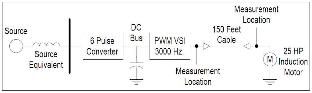
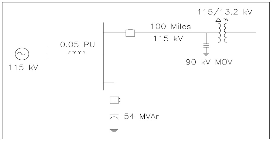
Drives for most small and medium sized induction motors may utilize voltage source inverters (VSI) to provide variable frequency ac output. The common drive structure adopted by industry consists of an uncontrolled diode-bridge rectifier, dc link, and PWM VSI inverter as shown in Figure 1. The dc link for the VSI type drive is basically a ripple smoothing capacitor. The inverter output waveform is generated by a series of step-like functions. Stray parameters of the circuit and commutation of switching devices from one phase to another prevent an ideal step-change in the output voltage. Steep-front waveform generation is one of the inherent characteristics of a high frequency operation voltage source inverter.
Figure 1 – Oneline Diagram Showing Power System and PWM Circuit
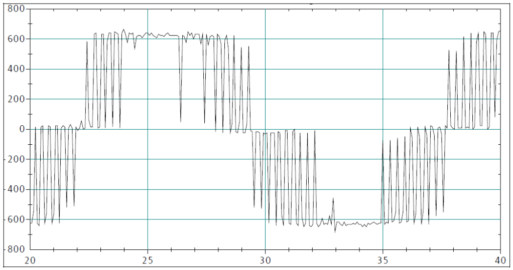
Both frequency and magnitude of the output voltage are adjusted by controlling the inverter’s operation. State of the art VSIs are based on IGBT technology. With IGBT devices, the inverter operates with a switching frequency ranging from tens of Hz to tens of thousands of Hz. Figure 2 illustrates the typical output voltage of a PWM drive. The switching frequency of the most commonly used PWM drives is in the range of 1000 Hz to 5000 Hz. The rise times of the pulses for IGBT VSIs can be on the order of 10μs to 0.1μs.
Figure 2 – Measured Line-to-Line Output Voltage of a Typical PWM ASD
THE PROBLEM
The problem occurs on the output of the ASD at the drive terminals. The high switching frequency of IGBTs allows sophisticated PWM schemes to be implemented. One of the advantages of the high switching frequency inverter is the reduction of low order harmonics, which results in the reduction of the output filter requirements. However, this benefit can only be achieved under certain circuit conditions. Under some particular conditions, the fast changing voltage resulting from high frequency switching operation of IGBT VSIs can create severe insulation problems for an induction motor.
Machine insulation integrity is affected by the rate of change of voltage as well as the over voltage magnitude. A voltage with a high rate of change tends to be distributed along a motor’s winding unevenly. This uneven distribution causes a significant over-stress across ending turns resulting in turn-to-turn insulation failure. In practice, it is common for the drive and the motor to be separated by long lengths of cable. Usually, the characteristic impedance of the motor can be ten to one hundred times that of the characteristic impedance of the cable connecting the drive to the motor.
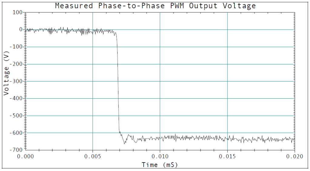
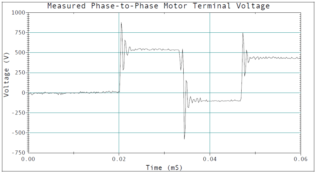
The most harmful effect of the PWM ASD output occurs when the connection cable is relatively long with respect to the wave front of an incidental voltage wave and when the ratio of characteristic impedance of the machine and the cable is high. In the worst case, an inverter output voltage pulse magnitude can be doubled at the induction motor terminals. Figure 3 illustrates one pulse transition as measured at the output of the ASD. Figure 4 illustrates several pulse transitions as measured at the terminals of an induction motor being supplied by an ASD. Notice the overshoot at the beginning and end of each pulse.
Figure 3 – Voltage Measured at Output of an ASD Feeding an Induction Motor.
Figure 4 – Voltage Measured at Motor Terminals of a Motor fed by an ASD.
THE SOLUTION
There are many potential mitigation techniques which might be employed to solve the over voltage problem at the motor terminals. With the proven EMTP simulation model, effectiveness of two promising solution methods were explored. These two methods are:
Install a line choke, in series with the connection cable, on the output of the PWM drive.
Install a capacitor, in parallel with the motor, at the motor terminals.
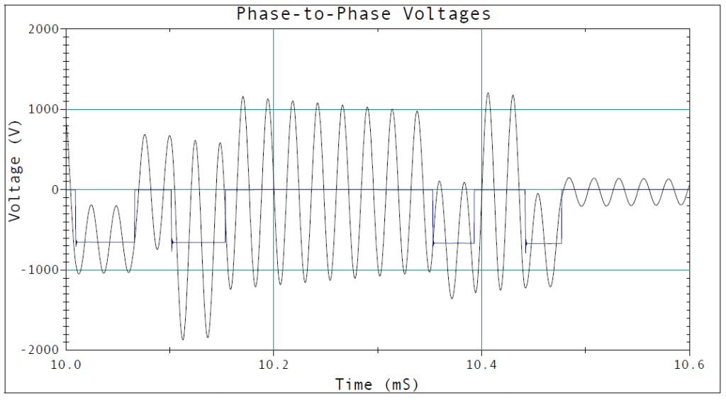
To evaluate the choke solution, a 5% (on the base of the 25 hp motor) inductor was inserted between the drive output and the connecting cable at the drive output terminals. The resulting phase-to-phase voltages at the drive output terminals and at the motor terminals are plotted together in. This ac output choke failed to control motor terminal over voltage as illustrated in Figure 5.
Figure 5 – Phase-to-Phase Voltage at Drive Output and Motor Terminals
The choke inductance did help to reduce the rate of change of the voltage seen by the motor. However, the choke created an extra circuit mesh which formed its current loop through the inverter source, choke inductance and cable equivalent capacitance.
The idea of installing capacitance at the motor terminal is initially drawn from the concept of matching the cable surge impedance with the characteristic impedance seen at the motor terminals. However, a precise matching of the impedance may require an amount of capacitance which is undesired for overall system consideration. Therefore, a compromise solution is to add some amount of capacitance to reduce the motor terminal characteristic impedance, and to introduce the proper level of damping to control the voltage overshoot. Based on this concept, three basic damping circuits can be used. They are:
An over damped circuit
A critically damped circuit
An under damped circuit
Each circuit includes a resistance in series with a capacitor. This series combination will be in parallel with the motor’s windings. The EMTP simulations showed that the best results were obtained when a critically damped circuit was employed at a properly selected resonant frequency. This method assures that the pulse at the end of the cable more closely matches the pulse at the beginning of the cable.
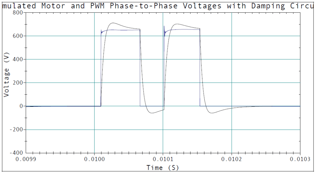
Knowing the switching frequency of the PWM drive was 3000 Hz and based on practical experience, it was decided that a good resonant frequency for the damping circuit would be five times the switching frequency or 15,000 Hz. Using the inductance of the cable (0.027mH for 150 ft. of # 8 AWG) the value of the capacitance was calculated to be 4.2μF and the damping resistance was selected to be 5.5 ohms. This circuit’s damping resistance was calculated based on 15,000 Hz.
Figure 6 – Simulated Phase-to-Phase Voltage at PWM Output Terminals with Damping Circuit
Figure 6 illustrates the effect that the introduced RC circuit has on the voltage at the motor terminals. The negligible over shoot in the voltage waveform illustrates that the circuit is slightly under damped. However, this approach does seem to have some merit. The high voltage reflection at the motor terminals is well under control and the over voltage is less than 1.2 per-unit. But, even more importantly, the steep front of the voltage pulse has been greatly reduced.
SUMMARY
When retrofitting induction motors with PWM ASDs, care must be taken in the length of the cable feeding the motor. Cases have been reported where a cable length as short as fifty feet caused a transients problem at the motor terminals. Conversely, there have been cases where the cable length was over 200 feet without adverse effects. If the problem is detected, an effective solution is to parallel an RC branch right at the motor terminals. Parameter selection for this RC branch is based on the drive circuit information and should be determined on case-by-case basis.
ASD manufacturers are now working with motor manufacturers to match drive duty motors to their drives. The ASD and motor come as a complete package. In fact, some motor manufacturers will not honor warranties for motors that are driven by PWM ASDs. And, in the case of new installations, require that the drive and motor be purchased as a package. The induction motors are designed to withstand the severe duties imposed on them by the high switching frequencies of the PWM drives.
REFERENCES
[1] Melhorn, C. J., Le Tang, “Transient Effects of PWM Drives on Induction Motors,” IEEE Transactions on Industry Applications, Volume 33, Number 4, July/August 1997. [2] Persson, E., “Transient effects in application of PWM inverters to induction motors,” presented at the IEEE/IAS 1991 Pulp and Paper Industry Conf., Montreal, P.Q., Canada, June 3-7, 1991, Paper PID 91-28.
GLOSSARY AND ACRONYMS ASD: Adjustable-Speed Drive PWM: Pulse Width Modulation VSI: Voltage Source Inverter
Published by Alena OTCENASOVA, Juraj ALTUS, Petr HECKO, Marek ROCH, Slovakia, University of Zilina, Faculty of Electrical Engineering, Department of Power Electrical Systems
Abstract. Worsened quality of supplied as well as demanded electricity causes in reality a large financial loss. The main quality parameters monitored today are voltage dips and interruptions. In this context there are relevant statistics of measurement results and especially the possibility of their improvement by using Dynamic Voltage Restorer, for which we have proposed a possible method of control. The proposed regulation DVR is based on Park transformation of immediate values of voltage in network and its feedback transformation. The method is shown and verified on simulation model.
Streszczenie. Pogorszenie jakości dostarczanej jak również zapotrzebowanej energii elektrycznej powoduje powstawanie dużych strat finansowych. Podstawowymi parametrami jakościowymi monitorowanymi obecnie są spadki napięcia i przerwy w zasilaniu. W tym kontekście istnieją adekwatn statystyki pomiarowe, a w szczególności możliwości ich poprawy poprzez użycie dynamicznego układu odtwarzania napięcia (DVR), dla którego zaproponowaliśmy metodę sterowania. Proponowana metoda sterowania układem DVR bazuje na transformacji Parka wartości chwilowych napięcia w sieci i ich transformacji odwrotnej. Metoda została przedstawiona i zweryfikowana na modelu symulacyjnym. (Pomiary parametrów napięcia w praktyce i możliwości poprawy jakości napięcia)
Keywords: power quality, electrical network, voltage dips and interruptions, dynamic voltage restorer, controlling of DVR. Słowa kluczowe: jakość energii, sieć elektryczna, spadki napięcia i przerwy w zasilaniu, dynamiczny układ odtwarzania napięcia, sterowanie układem DVR.
Introduction
Problems with power quality are always hot topic. The quality of electricity is influenced by many factors and to keep the parameters within the required limits is in many cases difficult. Worsened quality of electricity is often caused by customers by the nature of theirs operation. As they are in many cases supplied together with other customers from the point of common coupling it can lead to a situation where one customer’s device may retroactively influence also other customers. Likewise, negative influences can come from a distribution and from the transmission system too.
Study [1] focused on the problems with power quality prepared by the David Chapman from the Copper Development Association confirms that supplied electricity, whose quality does not satisfy relevant standards, causes huge economic losses. During resolving study David Chapman calculated concrete values of losses and says that the problems with power quality cost industry and business in the European Union around 10 billion euro per year.
Quality parameters of voltage
In general, power quality is evaluated according to the quality of electrical voltage. Basic characteristics of the quality parameters are given in the STN EN 50160 „Voltage characteristics of electricity supplied from the public distribution networks” [2]. This standard applies to low and medium voltage supply and is generally valid. It is applicable to electricity networks in European industrial areas, as well as the electricity network supplying the „two families isolated in the desert”.
This leads to various quality requirements. For many customers is the quality of voltage low even if it satisfies the requirements for quality according to STN EN 50160 and electricity is unusable (for example, the frequency of interruptions and voltage drops). Therefore stricter standards exist, for example STN EN 61000-2-2 and STN EN 61000-2-4 [3]. It is important that the customer has agreed properties of energy supplied according to the standards that match the type of operation with suppliers of electricity.
Standards that characterize quality parameters of electricity and specify the limits of parameters serve to ensure the functionality of devices supplied from this network, as well as devices that are connected to the network later [4].
Problems with quality of electricity in operating practice
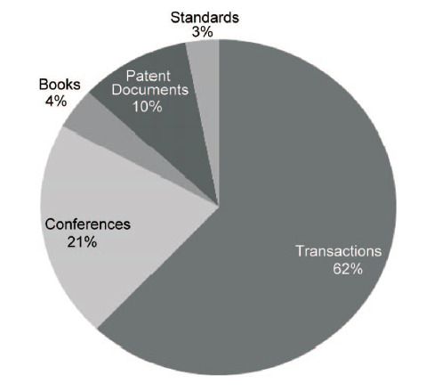
Power Grid Company [5] deals mainly with power quality measurement, delivery devices that increase the quality of electricity supply and distribution activities of components that are necessary for the production of compensation units, of low power electronics and semiconductors. Fig. 1 shows the statistical processing of various problems in industrial networks. These data are measurement results done by Power Grid Company [5] mainly in Slovakia and minor share in the Czech Republic.
Fig.1. Statistics of the most frequent problems measured by the Power Grid Company
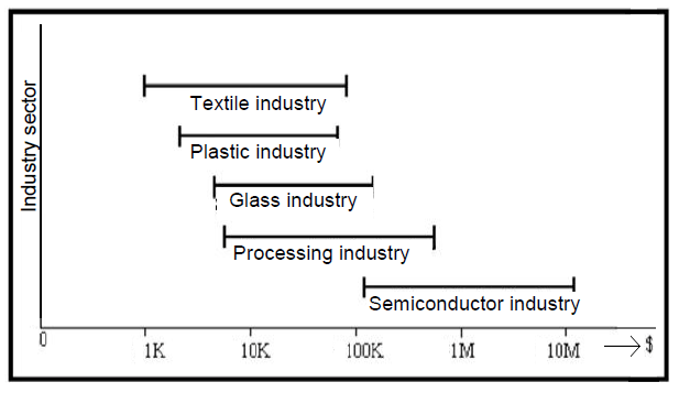
From the qualitative parameters listed in Fig. 1 dips and interruptions of supply voltage cause the highest economic losses [6]. Voltage dips and interruptions are especially dangerous for a group of customers, which are called the sensitive customers. For these customers even short time voltage dip may have the same economic impact as a long-term interruption of power supply. Examples of industries that are the most sensitive to the quality of power supply, including the costs to be paid on one fault (in dollars), are shown in Fig. 2 [6].
Fig.2. The cost of failure Voltage in the industry [6]
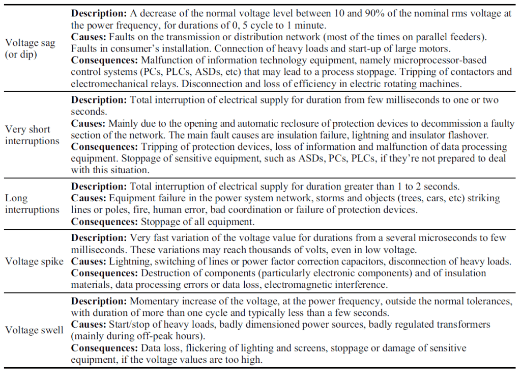
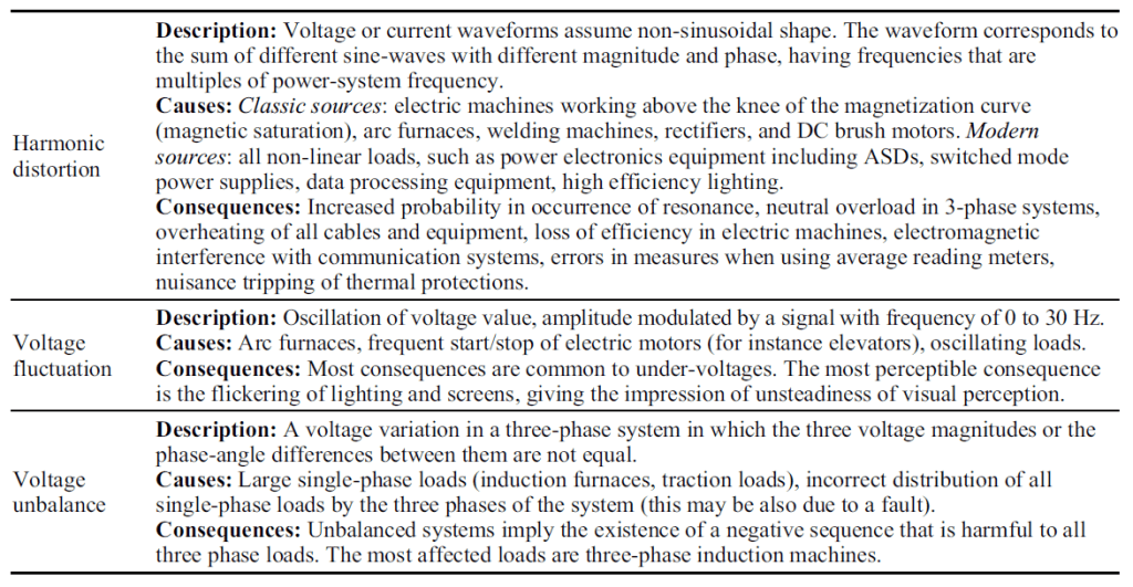
Dips (sags) and interruptions of voltage
Sags and interruptions belong among the quality attributes that can be easily identified by today’s network analysers. However solving problems is difficult, especially financially. As this can cause failure, damage to engine and also equipment, which results in considerable financial losses, increased attention is devoted to solving related issues. Their occurrence and frequency is random and are usually caused by external factors (weather, animals, vegetation, traffic accidents …). Statistics of interruptions and voltage drops of voltage (Fig.3) shows that in case of electricity the largest group is voltage dips from 10 to 30 % with duration from 10 to 100 ms.
Fig.3. Statistical processing of voltage dips [5]
In the operation, that deals with production cable harnesses for cars (cutting machine, foaming machine, ultrasonic welder, transporters, lighting, air conditioning, heating) there have been taken comparative measurements of power quality of network on 22 kV and 400 V sides of transformer in the substation MV on shorting terminal for invoice measurement.
At the same time short-term measurements were performed on the electronic board of the individual machines – foaming machine, ultrasonic welding, UPS, cutting machine. The problems presented by the client: power interruptions of electricity supply network – both short and long, voltage dips in the network – the consequent failure of production facilities. More dips, but also interruption in the L3 phase was recorded (Fig. 4) during network analysis.
The measurement was made simultaneously on the LV system and MV system, and therefore dips to low and middle voltage side can be compared. Comparison shows that dips and interruptions on LV side are always caused by dips and interruptions in the MV system.
Power Grid Company offers to solve the problem by installation of “Active voltage conditioner (AVC)”. AVC can eliminate a few seconds duration voltage sags and interruptions by defined way. The company offers several different AVC, which correspond to the different requirements for electric power.
Fig.4. Waveform of dip and interruption of voltage in phase L3 on MV side
AVC parameters are based on customer’s requirements on elimination of the dip length and its level and of course on desired power. The price of the equipment is highly dependent on AVC specifications. There is a possibility of AVC installation, which eliminates voltage failure for example 30 s for power several MV.A. Another possibility is for example use of industrial uninterruptible power supplies (UPS) where price is considerably higher.
The company can install UPS to machines that are most sensitive to power disturbances and therefore cause maximum economic damage. Another possibility is to supply the company from another power line which will supply company by energy in the case of primary source failure.
Another option, which will be discussed in the next part, is to compensate voltages dips and interruptions by Dynamic Voltage Restorer (DVR).
The principle of operation the DVR
Development of such compensation devices is connected with the development of power semiconductor devices. Basic connection of the DVR is in Fig. 5.
Fig.5. The principle of operation the DVR
The DVR is connected in series between the supply network and sensitive load. The voltage dips compensator is composed of single direct energy storage device, inverter, control circuit and a serial transformer. If the voltage dip appears on the supply side, the DVR will respond to this decline, and injects voltage into the network, which is needed to compensate accrued voltage dip. The result of this process is then constant voltage amplitude, which is to terminals of sensitive customer [6].
DVR control algorithms
The most important part in terms of proper function of the DVR is the correct control algorithm. The main function of the control algorithm is to keep required voltage value of sensitive loads in case of failure. Means of proceedings of real applied voltage compensators are “Know – how” of companies that install these devices. Various institutions such as universities, research institutes and specialized companies they are still exploring and testing new voltage compensators control algorithms. In general, it is difficult to design control algorithm, which could be generally applied and would also accept the economic aspects. Therefore, there are several control methods, and their application should be considered individually for each specific project.
There are several basic methods that are used in the control of compensators for dips and interruptions. These are the methods Pre-sag, In-phase and the newest method of Minimal Energy Control (controlling for the minimum energy) [7].
Model DVR based on the Park transformation
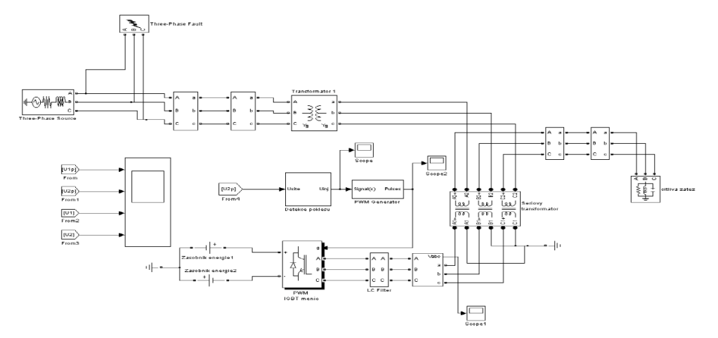
In terms of solving the problem of voltage dips, we have proposed a model DVR (Fig. 7). The control algorithm is based on the Park transformation.
Park’s transformation is the transformation connected with the rotor axis in theory of machines. It is also known as the transformation from abc, respectively αβ to dq0 components. Graphical presentation of Park transformation is shown in Fig. 6 [9].
Fig.6. Graphical presentation of Park transformation [9]
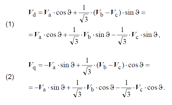
Park’s transformation is derived from the equations of Clarke transformation. When we derive equations as a base we use the equations for the calculation general stator variable [9]. Equations (1) and (2) represent mathematical description of the Park transformation:
.
The inverse Park’s transformation can be expressed by a similar procedure. For actual utilization in this paper there are presented only the final equations of the inverse Park transformation (6), (7) and (8).
Equations of Clarke and Park transformation are presented in different literatures in different modifications, while the principle remains the same. Simulation program Matlab/Simulink, which is used to simulate control DVR, calculates Park transformation using equations (3), (4) and (5):
.
Inverse (return) Park transformation is in MatLab described by equations (6), (7) and (8):
.
These equations are implemented into transformation blocks in Matlab/Simulink and are verified using computer simulations in the following part of article.
The principle of model operation DVR
The voltage that is measured in per units at the terminals appliance is transformed into dq0 components. We follow the theory that if the three-phase system is symmetrical, zero or q component does not develop after the Park transformation. If there is the asymmetry (for example the voltage dips in one phase) q component develops as well as the zero component. We compare this transformed value of voltage on appliance with dq0 constants, which represents a symmetrical system. If deviation occurs, the PI controllers regulate the deviation to zero. Then Park’s transformation is applied retroactively, and the resulting voltage is supplied into the PWM generator, which then sends impulses to the inverter, which creates the required voltage. Energy storage supplies inverter by power and it is created by direct ideal source. This voltage is then filtered by LC filter and through serial transformer injected into the network.
Verification of functions of the model DVR
To check correct DVR functioning there were simulated different disturbances and the response of monitored DVR. The DVR is designed and tested on the level of 22 kV, where it is normally installed.
For example, we present DVR reaction on the interphase short circuit that was simulated on the 110 kV voltage level at the time from 0.1 to 0.2 s. The resulting waveforms are shown in Fig. 8 and Fig. 9. In Fig. 8 is the voltage waveform displayed before DVR and the voltage waveform on the terminals of appliance is on the Fig. 9.
Fig.7. The model DVR in Matlab/simulink
Fig.8. The voltage waveform in supply network
Fig.9. The voltage waveform on the terminals of appliance
From the measured curves we can see that the customer has on its terminal constant value of voltage even if voltage failure occurs in the power supply network. It shows that DVR model fulfills its primary function and the proposed control algorithm works as we require from him.
Conclusion
In the article are described some results of measurements of the quality parameters of electricity with focus on voltage sags and interruptions. These disturbances cause significant financial losses for manufacturing companies. Therefore, there have been described ways how to prevent financial losses.
One of such methods is to install the Dynamic Voltage Restorer, which is closer specified in the article. The function of this voltage compensator has been verified by computer simulation and results confirm its proper operation. Installing the DVR is only theoretical with respect to its purchase price and the final choice of appropriate compensation is on the managers of the company.
Acknowledgment
This work was supported by European regional development fund (ERDF), name of project: Centre of excellence of power electronics systems and materials for their components, No.: OPVaV-2008/2.1/01-SORO, ITMS 26220120003.
REFERENCES
[1] Chapman, D., The cost of poor power quality. Power quality application guide. London, UK, 2001 [2] STN EN 50160 (33 0121). 2011. Voltage characteristics of electricity supplied by public electricity networks [3] STN EN 61000-2-4 (33 3432). 2003. Electromagnetic compatibility (EMC). Part 2-4: Environment – Compatibility levels in industrial plants for low-frequency conducted disturbances [4] Altus, J.,Novák, M.; Otčenášová, A.; Pokorný , M. , Electromagnetic compatibility of power systems, EDIS, publisher University of Zilina, SK, 2004, ISBN 80-8070-227-6 [5] http://www.power-grid.eu, + database Power Grid Company [6] Kuo, Y. Z.: Dynamic voltage restorer for sensitive equipment. Arlington, Texas. Dissertation thesis, 2007 [7] Dobrucký, B., Šul, R., Špánik, P., Zabezpečenie napájania kontinuálnych procesov s využitím zariadení FACTS. AT&P journal, Nov. 2005, pp. 79-81. [8] Hečko P. , Compensation voltage dips and interruptions in power station 110/25 kV, Žilina, Slovakia, Dissertation thesis, 2010 [9] Š t ěpina, J., Souměrné složky v teorii točivých elektrických strojů. Academia, Praha, 1969
Authors: prof. Ing. Juraj Altus, PhD., University of Zilina, Faculty of Electrical Engineering, Department of Power Electrical Systems, Univerzitná 1, 010 26 Žilina, Slovakia, E-mail: Juraj.Altus@fel.uniza.sk; doc. Ing. Alena Otčenášová, PhD., University of Zilina, Department of Power Electrical Systems, Alena.Otcenasova@fel.uniza.sk; Ing. Petr Hečko, E-mail: petrhecko@gmail.com.
Source & Publisher Item Identifier: PRZEGLĄD ELEKTROTECHNICZNY (Electrical Review), ISSN 0033-2097, R. 88 NR 9a/2012
Published by P. M. Balasubramaniam1 and S. U. Prabha2* 1Department of Electrical and Electronics Engineering, Sri Shakthi Institute of Engineering and Technology, Coimbatore, India 2Department of Electrical and Electronics Engineering, Sri Ramakrishna Engineering College, Coimbatore, India *Corresponding author. E-mail: baluanujayen@gmail.com
Abstract Classically, the aim of the electric power system is to generate electrical energy and to deliver this energy to the end-user equipment at an acceptable voltage. As nonlinear loads draw harmonic and reactive power components of current from ac mains, the quality of power deteriorates. This paper presents a review of the main power quality (PQ) problems with their associated causes and solutions with codes and standards. This paper concludes with some solutions to mitigate the Power Quality problems are presented.
Key words: IEEE 519, Total Harmonic Distortion, Point of Common Coupling, Total Demand Distortion
1. Introduction
Power quality (PQ) related issues are of most concern nowadays. The widespread use of electronic equipment, such as information technology equipment, power electronics such as adjustable speed drives (ASD), programmable logic controllers (PLC), energy-efficient lighting, led to a complete change of electric loads nature [1-3]. These loads are simultaneously the major causers and the major victims of power quality problems. Due to their non-linearity, all these loads cause disturbances in the voltage waveform.
Although many efforts have been taken by utilities, some consumers require a level of power quality higher than the level provided by modern electric networks [4]. This implies that some measures must be taken in order to achieve higher levels of power quality in Figure 1.
Figure 1. Sources of the review materials.
This paper provides an overview of major power quality issues, solutions and related standards based on an extensive number of publications. The referred publications are mainly extracted from IEEE transactions, IEEE Magazines, IEEE Proceedings, IEE/IET (Institution of Electrical Engineers, currently Institution of Engineering and Technology) Proceedings as well as a few, yet very important Conferences and patent documents on power quality and power quality improvement modules.
The review will be particularly useful for: 1) power system designers and researchers engaged in design, optimization, and quality-enhancement activities in today’s competitive environment; 2) practising engineers who would like to enrich their educational background about the system interaction aspects of power system for any application; and 3) undergraduate and postgraduate students who wish to integrate power quality issues and solutions with modern computing practices.
The paper starts with a short introduction to power quality issues (see section 2). In section 3, the solutions reviewed from various sources for power quality are given. A detailed literature review on codes and standards related to power quality are illustrated in sections 4. Finally, section 5 presents the summary and conclusions.
2. Types of Power Quality Issues
The most common types of power quality problems are presented in Table 1.
Table 1. Most common power quality issues [5-15]
.
Table 1. Continued
.
3. Solutions for Power Quality Issues
The mitigation of PQ problems may take place at different levels: transmission, distribution and the end-use equipment. Several measures can be taken at these levels are they are described in the following sections.
3.1 Grid Adequacy
Many PQ problems have origin in the transmission or distribution grid. Thus, a proper transmission and distribution grid, with adequate planning and maintenance, is essential to minimize the occurrence of PQ problems.
3.2 Unified Power Quality Conditioner (UPQC)
UPQC allows the alleviation of voltage and current disturbances that could affect sensitive electrical loads while compensating the load reactive power [16-19]. UPQC consists of combined series and shunt active power filters [20]. The main function of UPQC includes [21-25]:
(i) Reactive power compensation. (ii) Voltage regulation. (iii) Compensation for voltage sags and swells. (iv) Unbalance compensation for current and voltage (for 3-phase systems). (v) Neutral current compensation (for 3-phase 4-wire systems).
3.3 Distributed Resources – Energy Storage Systems
Interest in the use of distributed energy resources (DER) has increased substantially over the last few years because of their potential to provide increased reliability. These resources include distributed generation and energy storage systems. Energy storage systems, also known as restoring technologies, are used to provide the electric loads with ride-through capability in poor PQ environment. Recent technological advances in power electronics and storage technologies are turning the restoring technologies one of the premium solutions to mitigate PQ problems [26].
The first energy storage technology used in the field of PQ, yet the most used today, is electrochemical battery. Although new technologies, such as flywheels, Super-capacitors and Superconducting Magnetic Energy Storage (SMES) present many advantages, electrochemical batteries still rule due to their low price and mature technology [27].
3.4 Flywheels
A flywheel is an electromechanical device that couples a rotating electric machine (motor/generator) with a rotating mass to store energy for short durations. The motor/generator draws power provided by the grid to keep the rotor of the flywheel spinning. During a power disturbance, the kinetic energy stored in the rotor is transformed to DC electric energy by the generator, and the energy is delivered at a constant frequency and voltage through an inverter and a control system.
Traditional flywheel rotors are usually constructed of steel and are limited to a spin rate of a few thousand revolutions per minute (RPM). Advanced flywheels constructed from carbon fibre materials and magnetic bearings can spin in vacuum at speeds up to 40,000 to 60,000 RPM. The stored energy is proportional to the moment of inertia and to the square of the rotational speed. High speed flywheels can store much more energy than the conventional flywheels.
The flywheel provides power during a period between the loss of utility supplied power and either the return of utility power or the start of a back-up power system (i.e., diesel generator). Flywheels typically provide 1-100 seconds of ride-through time, and back-up generators are able to get online within 5-20 seconds.
3.5 Super-capacitors
Super-capacitors (also known as ultra-capacitors) are dc energy sources and must be interfaced to the electric grid with a static power conditioner, providing energy output at the grid frequency. A super-capacitor provides power during short duration interruptions or voltage sags. Medium size super-capacitors are commercially available to implement ride through capability in small electronic equipment, but large super-capacitors are still in development, but may soon become a viable component of the energy storage field [28,29].
Capacitance is very large because the distance between the plates is very small (several angstroms), and because the area of conductor surface (for instance of the activated carbon) reaches 1500-2000 m2/g (16000-21500 ft2/g). Thus, the energy stored by such capacitors may reach 50-60 J/g [30-38].
3.6 Superconducting Magnetic Energy Storage (SMES)
A magnetic field is created by circulating a DC current in a closed coil of superconducting wire. The path of the coil circulating current can be opened with a solid-state switch, which is modulated on and off. Due to the high inductance of the coil, when the switch is off (open), the magnetic coil behaves as a current source and will force current into the power converter which will charge to some voltage level. Proper modulation of the solid-state switch can hold the voltage within the proper operating range of the inverter, which converts the DC voltage into AC power. Atypical SMES system.
Low temperature SMES cooled by liquid helium is commercially available [39,40]. High temperature SMES cooled by liquid nitrogen is still in the development stage and may become a viable commercial energy storage source in the future due to its potentially lower costs. SMES systems are large and generally used for short durations, such as utility switching events.
3.7 Enhanced Interface Devices
Using proper interface devices, one can isolate the loads from disturbances deriving from the grid. The common interface devices are dynamic voltage restorer (DVR), transient voltage surge suppressors (TVSS), constant voltage transformers (CVT), Noise Filters, Active Power Filters, Isolation Transformers, Static VAR Compensators (SVC), Harmonic Filters and reactor for power quality improvement.
A dynamic voltage restorer (DVR) acts like a voltage source connected in series with the load. The output voltage of the DVR is kept approximately constant voltage at the load terminals by using a step-up transformer and/or stored energy to inject active and reactive power in the output supply trough a voltage converter.
Transient voltage surge suppressors are used as interface between the power source and sensitive loads, so that the transient voltage is clamped by the TVSS before it reaches the load. TVSSs usually contain a component with a nonlinear resistance (a metal oxide varistor or a zener diode) that limits excessive line voltage and conduct any excess impulse energy to ground.
Constant voltage transformers (CVT) were one of the first PQ solutions used to mitigate the effects of voltage sags and transients. To maintain the voltage constant, they use two principles that are normally avoided: resonance and core saturation. Atypical constant voltage transformer. When the resonance occurs, the current will increase to a point that causes the saturation of the magnetic core of the transformer. If the magnetic core is saturated, then the magnetic flux will remain roughly constant and the transformer will produce an approximately constant voltage output. If not properly used, a CVT will originate more PQ problems than the ones mitigated. It can produce transients, harmonics (voltage wave clipped on the top and sides) and it is inefficient (about 80% at full load). Its application is becoming uncommon due to technological advances in other areas.
Noise filters are used to avoid unwanted frequency current or voltage signals (noise) from reaching sensitive equipment. This can be accomplished by using a combination of capacitors and inductances that creates a low impedance path to the fundamental frequency and high impedance to higher frequencies, that is, a low-pass filter. They should be used when noise with frequency in the kilo Hertz range is considerable.
Static VAR compensators (SVR) use a combination of capacitors and reactors to regulate the voltage quickly. Solid-state switches control the insertion of the capacitors and reactors at the right magnitude to prevent the voltage from fluctuating. The main application of SVR is the voltage regulation in high voltage and the elimination of flicker caused by large loads (such as induction furnaces).
Harmonic filters are used to reduce undesirable harmonics. They can be divided in two groups: passive filters and active filters [41-43]. Passive filters consist in a low impedance path to the frequencies of the harmonics to be attenuated using passive components (inductors, capacitors and resistors). Several passive filters connected in parallel may be necessary to eliminate several harmonic components [44]. If the system varies (change of harmonic components), passive filters may become ineffective and cause resonance.
Active filters analyse the current consumed by the load and create a current that cancel the harmonic current generated by the loads. Active filters were expensive in the past, but they are now becoming cost effective compensating for unknown or changing harmonics [45].
Reactor for power quality improvement is a patented technology [46-49]. The device is installed on a power line, for removing noise that flows into the power line, characterized by: a reactor having a first coil and a second coil wound on a core disposed between the input end and the output ends of the power line, wherein in the reactor the first end of the first coil is connected to the input end of a first power line, the second end of the first coil is connected to the output end of the first power line, and the first end of the second coil is connected to the output end of the second power line, and the second end of the second coil is connected to the input end of the second power line.
3.8 Make End-use Devices Less Sensitive
Designing the equipment to be less sensitive to disturbances is usually the most cost effective measure to prevent PQ problems. Some manufacturers of end-use equipment are now recognising this problem, but the competitive market means that manufacturers should reduce costs and only respond to customers’ requirements. The exception is the ASD market, where manufacturers are actively promoting products with enhanced ride-through capabilities.
Some of the energy meters have the capability for power quality detection, monitoring, reporting, recording and communication in a revenue accuracy electrical power meter is disclosed [50]. Transient events are detected by monitoring the Wave shape of the electrical power and comparing deviations to a known threshold. Sags and Swells are detected by computing root mean square value over a rolling Window and comparing the computed value with a known threshold. Harmonic frequencies and symmetrical components are quantified by a known algorithm and compared with a known threshold [51]. Adding a capacitor with a larger capacity to power supplies, using cables with larger neutral conductors, derating transformers and adjusting under voltage relays, are measures that could be taken by manufacturers to reduce the sensitivity of equipment to PQ problems.
4. Codes and Standards
Some measures have been taken to regulate the minimum PQ level that utilities have to provide to consumers and the immunity level that equipment should have to operate properly when the power supplied is within the standards. Standardization organizations like IEC, CENELEC, and IEEE have developed a set of standards with the same purposes. In Europe, the most relevant standards in PQ are the EN 50160 (by CENELEC) and IEC 61000. IEEE power quality standards do not have such a structured and comprehensive set as compared to IEC [52]. Nonetheless, the IEEE standards give more practical and some theoretical background on the phenomena, which makes it a very useful reference. Some of the IEEE power quality standards are described in the ensuing sections.
4.1 IEEE 519
Power system problems that were associated with harmonics began to be of general concern in the 1970s, when two independent developments took place. The first was the oil embargo, which led to price increases in electricity and the move to save energy. Industrial consumers and utilities began to apply power factor improvement capacitors. The move to power factor improvement resulted in a significant increase in the number of capacitors connected to power systems. American standards regarding harmonics have been laid out by the IEEE in the 519 Standard: IEEE Recommended Practices and Requirements for Harmonic Control in Electric Power Systems. There is a combined effect of all nonlinear loads on utility systems that have a limited capability to absorb harmonic current. Further, utilities are charged with the responsibility to provide a high quality supply in terms of voltage level and waveform. IEEE 519 recognizes not only the absolute level of harmonics produced by an individual source but also their size relative to the supply network. It should be noted that IEEE 519 is limited to being a collection of Recommended Practices that serve as a guide to both suppliers and consumers of electrical energy. Where problems exist, because of excessive harmonic current injection or excessive voltage distortion, it is incumbent upon supplier and consumer to resolve the issues within a mutually acceptable framework [53].
4.2 IEEE 519 Standard for Harmonic Voltage Limits
According to IEEE 519 Table 2 shows that, harmonic voltage distortion on power system 69 kV and below is limited to 5% Total Harmonic Distortion with each individual harmonic limited 3% [54].
Table 2. Harmonic voltage distortion limits
.
4.3 IEEE 519 Standard for Harmonic Current Limits
General distribution systems [GDS 120V-69,000 V]: Current distortion limits are for odd harmonics. Even harmonics are limited to 25% of the odd Harmonic limits. For all power generation equipment, distortion limits are those with ISC/IL < 20. ISC is the maximum short circuit current at the point of coupling “PCC”. IL is the maximum fundamental frequency 15-or 30- minutes load current at PCC. TDD is the total demand distortion (= THD normalized by IL are shown in Table 3).
Table 3. Harmonic current distortion limits
.
General sub-transmission systems [GSTS 69 kV-161 kV]: The current harmonic distortion limits apply to limits of harmonics that loads should draw from the utility at the PCC. Note that the harmonic limits differ based on the ISC/IL rating, where ISC is the maximum short circuit current at the PCC, and I is the maximum demand load current at the PCC.
ISC is the available short circuit current at the point of common coupling. The ISC is determined by the size, impedance, and voltage of the service feeding the PCC. IL is the maximum demand load current (fundamental frequency component) measured at the PCC are shown in Table 4. It is suggested that existing facilities measure this over a period of time and average it. Those creating new designs should calculate the IL using anticipated peak operation of the facility. The point of common coupling with the consumer/utility interface is the closest point on the utility side of the customer service where another utility service customer is or could be supplied. The ownership of any apparatus such as a transformer that the utility might provide in the customers system is immaterial to the definition of PCC. This definition has been approved by IEEE working group.
Table 4. Maximum harmonic current distortion level
.
4.4 IEEE Standard 142-1991, Recommended Practice for Grounding of Industrial and Commercial Power Systems [55]
This standard presents a thorough investigation of the problems of grounding and the methods for solving these problems. There is a separate chapter for grounding sensitive equipment.
4.5 IEEE Standard 446-1987, Recommended Practice for Emergency and Standby Power Systems for Industrial and Commercial Applications
This standard is recommended engineering practices for the selection and application of emergency and standby power systems. It provides facility designers, operators and owners with guidelines for assuring uninterrupted power, virtually free of frequency excursions and voltage dips, surges, and transients.
4.6 IEEE Standard 1100-1999, Recommended Practice for Powering and Grounding Sensitive Electronic Equipment
Recommended design is installation, and maintenance practices for electrical power and grounding (including both power-related and signal-related noise control) of sensitive electronic processing equipment used in commercial and industrial applications.
4.7 IEEE Standard 1346-1998 Recommended Practice for Evaluating Electric Power System Compatibility with Electronic Process Equipment
A standard methodology for the technical and financial analysis of voltage sag compatibility between process equipment and electric power systems is recommended. The methodology presented is intended to be used as a planning tool to quantify the voltage sag environment and process sensitivity.
4.8 IEEE Standards Related to Voltage Sag and Reliability
The distribution voltage quality standard i.e. IEEE Standard P1564 gives the recommended indices and procedures for characterizing voltage sag performance and comparing performance across different systems. A new IEC Standard 61000-2-8 titled “Environment – Voltage Dips and Short Interruptions” has come recently. This standard warrants considerable discussion within the IEEE to avoid conflicting methods of characterizing system performance in different parts of the world.
4.9 IEEE Standards Related to Flicker
Developments in voltage flicker standards demonstrate how the industry can successfully coordinate IEEE and IEC activities. IEC Standard 61000-4-15 defines the measurement procedure and monitor requirements for characterizing flicker. The IEEE flicker task force working on Standard P1453 is set to adopt the IEC standard as its own.
4.10 Standards Related to Custom Power
IEEE Standard P1409 is currently developing an application guide for custom power technologies to provide enhanced power quality on the distribution system. This is an important area for many utilities that may want to offer enhanced power quality services.
4.11 Standards Related to Distributed Generation
The new IEEE Standard P1547 provides guidelines for interconnecting distributed generation with the power system.
4.12 420-2013 – IEEE Standard for the Design and Qualification of Class 1E Control Boards, Panels and Racks Used in Nuclear Power Generating Stations
This standard specifies the design requirements for new and/or modified Class 1E control boards, panels, and racks and establishes the methods to verify that these requirements have been satisfied. Methods for meeting the separation criteria contained in IEEE Std 384 are addressed. Qualification is also included to address the overall requirements of IEEE Std 323 and recommendations of IEEE Std 344.
4.13 IEEE Standard 384-2008 – IEEE Standard Criteria for Independence of Class 1E Equipment and Circuits
The independence requirements of the circuits and equipment comprising or associated with Class 1E systems are described. Criteria for the independence that can be achieved by physical separation and electrical isolation of circuits and equipment that are redundant are set forth. The determination of what is to be considered redundant is not addressed.
4.14 IEEE Standard C57.18.10-1998 – IEEE Standard Practices and Requirements for Semiconductor Power Rectifier Transformers
Practices and requirements for semiconductor power rectifier transformers for dedicated loads rated single-phase 300 kW and above and three-phase 500 kW and above are included. Static precipitators, high-voltage converters for DC power transmission, and other nonlinear loads are excluded. Service conditions, both usual and unusual, are specified, or other standards are referenced as appropriate. Routine tests are specified. An informative annex provides several examples of load loss calculations for transformers when subjected to non-sinusoidal currents, based on calculations provided in the standard.
4.15 IEEE Standard C57.21-1990 -IEEE Standard Requirements, Terminology and Test Code for Shunt Reactors Rated Over 500 kVA
All oil-immersed or dry-type, single-phase or three phase, outdoor or indoor shunt reactors rated over 500 kVA are covered. Terminology and general requirements are stated, and the basis for rating shunt reactors is set forth. Routine, design, and other tests are described, and methods for performing them are given. Losses and impedance, temperature rise, dielectric tests, and insulation levels are covered. Construction requirements for oil immersed reactors and construction and installation requirements for dry-type reactors are presented.
5. Summary and Conclusions
This paper gives a comprehensive review by critical analyzing about power quality problems, issues, related international standards, and the solutions. The correct solutions are also discussed which can be remedy for power quality problems generated in different phenomena. Coordination with existing industry practices and international harmonic standards is also considered in this paper. To overcome the negative impact of poor power quality on equipment and businesses, suitable power quality equipment can be invested. Identifying the right solution remains the first step. Many power quality problems are easily identified once a good description of the problems is obtained. Unfortunately, the tensions caused by power problems often result in vague or overly dramatic descriptions of the problem.
A power quality audit can help determine the causes of your problems and provide a well designed plan to correct them. The power quality audit checks the facility’s wiring and grounding to ensure that it is adequate for your applications and up to code. The auditor normally will check the quality of the ac voltage itself, and consider the impact of the utility’s power system. Many businesses and organizations rely on computer systems and other electrical equipment to carry out the mission critical functions, but they aren’t safeguarding against the dangers of an unreliable power supply. It is time utilities as well as businesses engage in more proactive approach to power quality treats by engaging in power quality analysis.
References
[1] Bollen, M., “Understanding Power Quality Problems – Voltage Sags and Interruptions”, IEEE Press Series on Power Engineering – John Wiley and Sons, Piscataway, USA(2000). doi: 10.1109/9780470546840.ch4 [2] Rajakumar, P., et al., Review on Power Quality Issues, IRACST – Engineering Science and Technology: An International Journal (ESTIJ), ISSN: 2250-3498, Vol.2, No. 1 (2012). [3] Delgado, J., Gestão da Qualidade Total Aplicada ao Sector do Fornecimento da Energia Eléctrica, Ph. D. Dissertation Electrotechnical Engineering, Universidade de Coimbra, Portugal September (2002). [4] Choi, W. Y., Kwon, J., Kim, E. H., Lee, J. J. and Kwon, B. H., “Bridgeless Boost Rectifier with Low Conduction Losses and Reduced Diode Reverse Recovery Problems,” IEEE Trans. Ind. Electron., Vol. 54, No. 2, pp. 769 – 780 (2007). doi: 10.1109/TIE.2007.891991 [5] Lin, T., Domijan, A., Jr. and Chu, F., “A Survey of Techniques for Power Quality Monitoring,” Int. J. Power Energy Syst., Vol. 25, No. 3, pp. 167-172 (2012). [6] Chen, G., Chen, Y. and Smedley, K. M., “Three-phase Four-leg Active Power Quality Conditioner without References Calculation,” Proc. Appl. Power Electron. Conf., pp. 587-593 (2004). doi: 10.1109/APEC.2004. 1295866 [7] López, Y.-K., de Vicuña, L. G., Castilla, M., Matas, J. and López, M., “Sliding-mode-control Design of a High-power-factor Buck-boost-rectifier,” IEEE Trans. Ind. Electron., Vol. 46, pp. 604-612 (1999). [8] Mollov, S. V. and Forsyth, A. J., “Analysis, Design and Resonant Current Control for a 1-MHz High – powerfactor Rectifier,” IEEE Trans. Ind. Electron., Vol. 46, pp. 620-627 (1999). doi: 10.1109/41.767070 [9] García, A. J., Cobos, J. A., Prieto, R., Alou, P. and Uceda, J., “An Alternative to Supply DC Voltages with High Power Factor,” IEEE Trans. Ind. Electron., Vol.46, pp. 703-709 (1999). doi: 10.1109/41.778219 [10] Lee, J.-Y., Moon, G.-W. and Youn, M.-J., “Design of a Power-factor-Correction Converter Based on Halfbridge Topology,” IEEE Trans. Ind. Electron., Vol. 46, pp. 710-723 (1999). doi: 10.1109/41.778222 [11] Madigan, M. T., Erickson, R.W. and Ismail, E. H., “Integrated High-quality Rectifier-regulators,” IEEE Trans. Ind. Electron., Vol. 46, pp. 749-758 (1999). doi: 10.1109/41.778229 [12] Wu, T.-F. and Chen, Y.-K., “Analysis and Design of an Isolated Single Stage Converter Achieving Power factor Correction and Fast Regulation,” IEEE Trans. Ind. Electron., Vol. 46, pp. 759-767 (1999). doi: 10.1109/41.778230 [13] Hsieh, G.-C. andWang, C.-M., “ZCS-PWM Full-wave Boost Rectifier with Unity Power Factor and Low Conduction Losses,” IEEE Trans. Ind. Electron., Vol. 46, pp. 768-779 (1999). doi: 10.1109/41.778234 [14] Tseng, C.-J. and Chen, C.-L., “ANovel ZVT PWMCúk Power-factor Corrector,” IEEE Trans. Ind. Electron., Vol. 46, pp. 780-787 (1999). doi: 10.1109/41.778240 [15] Ferracci, P., “Power Quality,” Schneider Electric Cahier Technique, No. 199, September (2012). [16] Zhu, P., Li, X., Kang, Y. and Chen, J., “A Novel Control Scheme in 2-phase Unified Power Quality Conditioner,” in Proc. 29th Annu. Conf. IEEE Ind. Electron. Soc., pp. 16917-1622 (2003). doi:10.1109/TIE.2014.2314055 [17] Ghosh, A., Jindal, A. K. and Joshi, A., “Modified Power Quality Conditioner for Voltage Regulation of Critical Load Bus,” Proc. Power Eng. Soc. Gen. Meet., pp. 471-476 (2004). doi: 10.1109/PES.2004.1372840 [18] Cheng, Y. and Philippe, L., “Advanced Control Methods for the 3-phase Unified Power Quality Conditioner,” Proc. Power Electron. Spec. Conf., pp. 4263-4267 (2004). doi: 10.1109/PESC.2004.1354754 [19] Tlusty, J. and Valouch, V., “Effectiveness of Unified Power Quality Conditioner for Flicker Mitigation,” Proc. 4th Int. Power Electron. Motion Control Conf. , pp. 902-907 (2004). [20] Khadkikar, V., Agarwal, P., Chandra, A., Barry, A. and Nguyen, T., “A Simple New Control Technique for Unified Power Quality Conditioner (UPQC),” Proc. 11th Int. Conf. Harmonics Quality Power, pp. 289-293 (2004). doi: 10.1109/ICHQP.2004.1409369 [21] Esfandiari, A., Parniani, M. and Mokhtari, H., “Mitigation of Electric Arc Furnace Disturbances Using the Unified Power Quality Conditioner,” Proc. 30th Annu. Conf. Ind. Electron. Soc., pp. 1469-1474 (2004). doi: 10.1109/IECON.2004.1431795 [22] Sepulveda, C. A., Espinoza, J. R., Moran, L. A. and Ortega, R., “Analysis and Design of a Linear Control Strategy for Three-phase UPQCs,” Proc. 30th Annu. Conf. IEEE Ind. Electron. Soc., Vol. 3, pp. 3060-3065 (2004). doi: 10.1109/IECON.2004.1432300 [23] Ng, F., Wong, M. C. and Han, Y. D., “Analysis and Control of UPQC and its DC-link Power by Use of pq-r Instantaneous Power Theory,” Proc. Power Electron. Syst. Appl., pp. 43-53 (2004). doi: 10.1109/TPEL. 2004.826499 [24] Tey, L. H., So, P. L. and Chu, Y. C., “Unified Power Quality Conditioner for Improving Power Quality Using ANN with Hysteresis Control,” Proc. Int. Conf. Power Syst. Technol., pp. 1441-1446 (2004). doi: 10. 1109/ICPST.2004.1460229 [25] Vinod Khadkikar, Enhancing Electric Power Quality Using UPQC: AComprehensive Overview, IEEE Transactions on Power Electronics, Vol. 27, No. 5 (2012). doi: 10.1109/TPEL.2011.2172001 [26] Ribeiro, P., Johnson, B., Crow, M., Arsoy, A. and Liu, Y., “Energy Storage Systems for Advanced Power Applications,” Proceedings of the IEEE, Vol. 89, No. 12, (2001). doi: 10.1109/5.975900 [27] Kwon, J. M., Choi, W. Y. and Kwon, B. H., “Cost-effective Boost Converter with Reverse-recovery Reduction and Power Factor Correction,” IEEE Trans. Ind. Electron., Vol. 55, No. 1, pp. 471-473 (2008). doi: 10.1109/TIE.2007.896526 [28] Tofoli, F. L., Coelho, E. A. A., de Freitas, L. C., Farias, V. J. and Vieira, J. B. Jr., “Proposal of a Soft-switching Single-phase Three-level Rectifier,” IEEE Trans. Ind. Electron., Vol. 55, No. 1, pp. 107-113 (2008). doi: 10. 1109/TIE.2007.896052 [29] IEEE Recommended Practice for Monitoring Electric Power Quality, IEEE Std. 1159-2009 (2009). [30] Ghosh, A., Jindal, A. K. and Joshi, A., “Inverter Control Using Output Feedback for Power Compensating Devices,” Proc. Convergent Technol. Conf. , pp. 48-52 (2003). doi: 10.1109/TENCON.2003.1273212 [31] Rodríguez, E., Abud, D. and Arau, J., “ANovel Singlestage Single-phase DC Uninterruptible Power Supply with Power-factor Correction,” IEEE Trans. Ind. Electron., Vol. 46, pp. 1137-1147 (1999). doi: 10.1109/41.808002 [32] Alonso, J. M., Calleja, A. J., López, E., Ribas, J. and Scades, M. R., “A Novel Single-stage Constant-wattage High-power-factor Electronic Ballast,” IEEE Trans. Ind. Electron., Vol. 46, pp. 1148-1158 (1999). doi: 10.1109/41.808004 [33] Pires, V. F. and Silva, J. F., “Half-bridge Single-phase Buck-boost Type AC-DC Converter with Sliding Mode Control of the Input Source Current,” Proc. IEE-Elect. Power Applicat., Vol. 147, No. 1, pp. 61-67 (2000). doi: 10.1049/ip-epa:20000020 [34] Siu, K.-W. and Lee, Y.-S., “A Novel High-efficiency Flyback Power-factor Correction Circuit with Regenerative Clamping and Soft Switching,” IEEE Trans. Circuits Syst. I, Vol. 47, pp. 350-356 (2000). doi: 10.1109/81.841917 [35] Matsui, K., Yamamoto, I., Hirose, S., Ando, K. and Kobayashi, T., “Utility-Interactive Photovoltaic Power Conditioning Systems with Forward Converter for Domestic Applications,” Proc. IEE-Elect. Power Applicat., Vol. 147, No. 3, pp. 199-205 (2000). doi: 10.1049/ipepa:20000374 [36] Buso, S., Spiazzi, G. and Tagliavia, D., “Simplified Control Technique for High-power-factor Flyback Cuk and Sepic Rectifiers Operating in CCM,” IEEE Trans. Ind. Applicat., Vol. 36, pp. 1413-1418 (2000). doi: 10.1109/28.871291 [37] Anderson, G. K. and Blaabjerg, F., “Current Programmed Control of a Single Phase Two-switch Buckboost Power Factor Correction Circuit,” Proc. IEEE APEC’01, pp. 350-356 (2001). doi: 10.1109/APEC. 2001.911671 [38] Chen, J., Maksimovic, D. and Erickson, R., “A New Low-stress Buck-boost Converter for Universal-input PFC Applications,” Proc. IEEE APEC’01, pp. 343-349 (2001). [39] Amaro, N. and Ceballos, J. M., “A Fast Algorithm for Initial Design of HTS Coils for SMES Applications,” IEEE Transactions on Applied Superconductivity, Vol.23, No. 3 (2013). doi: 10.1109/TASC.2012.2231912 [40] Chen, X. Y. and Jin, J. X., “Development of SMES Technology and its Applications in Power Grid,” Proc. Int. Conf. Appl. Supercond. Electromagn. Dev., pp.260-269 (2011). doi: 10.1109/ASEMD.2011.6145115 [41] Singh, B., Al-Haddad, K. and Chandra, A., “A Review of Active Filters for Power Quality Improvement,” IEEE Transactions on Industrial Electronics, Vol. 46, No. 5 (1999). doi: 10.1109/41.793345 [42] Singh, B., Al-Haddad, K. and Chandra, A., “A Review of Active Filters for Power Quality Improvement,” IEEE Trans. Ind. Electron., Vol. 46, No. 5, pp. 960-971 (2012). doi: 10.1109/41.793345 [43] Active Filters: Technical Document, 2100/1100 Series, Mitsubishi Electric Corp., Tokyo, Japan, pp. 1-36 (1989). [44] Kikuchi, A. H., “Active Power Filters,” in Toshiba GTRModule (IGBT) Application Notes, Toshiba Corp., Tokyo, Japan, pp. 44-45 (1992). [45] Gyugyi, L. and Strycula, E., “ActiveAC Power Filters,” in Conf. Rec. IEEE-IAS Annu. Meeting, pp. 529-535 (1976). [46] Inventor: KIM, Seon Ho Daejeon Metropolitan City 301-030 (KR), Device For Improving Power Quality, European Patent Application Number: 11809896.1, Date of Filing: 22.07.2011. [47] US Patent N0.: US 6,615,147 B1, Date of Patent: Sep.2, Inventors: Rene T. J. Onker, British Columbia, Invention: Revenue Meter with Power Quality Features (2003). [48] US Patent No.: US 8,326,576 B2, Date of Patent: Dec. 4, Inventor: Man-0n Pun, Cambridge, MA(U S), Invention: Detecting Power Quality Events in Power Distribution Networks (2012). [49] US Patent No.: WO 2011124223 A3, Date of Patent: Nov 29, Inventor(s): Lucian Asiminoaei, Sergej Kalaschnikow, Invention: Power Quality Improvement by Active Filter (2012). [50] Revenue Meter with Power Quality Features, Patent N0.: US 6,615,147 B1, Date of Patent: Sep. 2, Inventor: Rene T. J. Onker, British Columbia (2003). [51] Routimo, M., Salo, M. and Tuusa, H., “Improving the Active Power Filter Performance with a Prediction Based Reference Generation,” Nordic Workshop on Power and Industrial Electronics, Norpie (2004). [52] IEEE Standard 446-1987, “IEEE Recommended Practice for Emergency and Standby Power Systems for Industrial and Commercial Applications,” (IEEE Orange Book). doi: 10.1049/pe:19890012 [53] IEEE Std 1250-1995, “IEEE Guide for Service to Equipment Sensitive to Momentary Voltage Disturbances,” Art 5.1.1, Computers. [54] IEEE, “IEEE Guide for Service to Equipment Sensitive to Momentary Voltage Disturbances,” IEEE Std. 1250-1995. [55] IEEE Recommended Practice for Grounding of Industrial and Commercial Power Systems, 142-1991 (1992). doi: 10.1049/pe:19890012
Published by Electrotek Concepts, Inc., PQSoft Case Study: Phase-to-Phase Transients at Transformer Terminations During Utility Capacitor Switching, Document ID: PQS0603, Date: January 1, 2006.
Abstract: There are a number of important transient related concerns when transmission capacitor banks are applied. These concerns include insulation withstand level, switchgear capabilities, energy duties of protective devices, and system harmonic considerations. The considerations should also be extended to include distribution systems and sensitive customer equipment. This case study presents a summary of the model development and simulations results for a phase-to-phase transients at transformer terminations evaluation.
INTRODUCTION
Energizing a shunt capacitor bank can subject three-phase transformers to excessive phase-to-phase and/or high frequency transients. The basic circuit configuration of concern consists of a three-phase transformer at one terminal of a radial line and a switched capacitor bank at the other terminal. The high phase-to-phase voltages are a result of traveling wave reflections at the transformer termination. It is possible to obtain transients approaching twice the peak system voltage on two phases with opposite polarity, resulting in a phase-to-phase transient of approximately four times the normal peak phase-to-ground voltage. These transients can easily exceed the phase-to-phase withstand capability of three phase transformers.
Figure 1 illustrates the simplified circuit used to investigate phase-to-phase transient voltages. Transient voltage problems at transformer terminations occur primarily with a delta primary winding fed radially from a capacitor location.
Figure 1 – Oneline Diagram for Analysis of Phase-to-Phase Overvoltages
Xs = ( 1152/100 ) ∗ 0.05 = 6.6125Ω, Ls = 17.54mH
Xc = ( 1152/54 ) = 244.907Ω, C = 10.83μF
The transient voltages that can occur must be evaluated with respect to the transformer phase-to-phase insulation withstand capability. The IEEE Trial Use Standard (IEEE Std. 262B) for transformers specifies a phase-to-phase switching surge insulation level for transformers at 345kV and above. For transformers on 345kV systems, the recommended switching surge insulation level is 1050kV or 3.73 per-unit. No guidelines exist for lower voltage transformers. A worst-case assumption would be that the phase-to-phase insulation level is equal to the phase-to-ground insulation level.
MODEL DEVELOPMENT
The study of utility capacitor switching events frequently requires the use of sophisticated digital simulation tools. Simulations provide a convenient means to characterize transient events, determine resulting power quality problems, and evaluate possible mitigation methods. Quite often, they are performed in conjunction with system monitoring for verification of models and identification of important power quality concerns. The complexity of the models required for the simulations depends on the system characteristics and the transient event under investigation.
There are a number of important system variables that influence the phase-to-phase transient voltage magnitude that can occur at a transformer termination during capacitor switching. They include:
− Source characteristic: The source characteristic at the switched capacitor bank includes the short circuit capacity and the number of transmission lines entering the substation.
− Switched capacitor ratings: As with varying the source impedance, varying the switched capacitor ratings changes the frequency of oscillation that occurs when the capacitor is energized.
− Radial line length: The length of the transmission line between the capacitor bank and the transformer is important because it determines the length of time (and frequency) it takes a traveling wave to traverse the line.
− Transformer location along radial line: The highest traveling wave overvoltages during capacitor switching generally occur at radial line terminations. However, there are often a number of transformers tapped off the radial circuit. Usually, transformers along most of the line can be exposed to phase-to-phase transient voltages which may be excessive in terms of the transformer insulation.
− Surge arresters: Surge arresters located at the transformer can help protect the transformer from excessive phase-to-phase transients. The maximum phase-to-phase transient is equal to twice the arrester protective level when arresters are connected line-to-ground.
The phase-to-phase withstand strength of transformers on the system will depend on a number of factors; including transformer type, BIL rating, and construction. A worst-case assumption regarding the phase-to-phase withstand is that it is equal to the transformer phase-to-ground withstand level (which is determined directly by the BIL rating). This assumption is reasonable for delta-wye transformers used to supply distribution substations. It is likely that autotransformers will have greater phase-to-phase insulation strength because there are no windings connected directly across the phases.
The transmission line was represented using the following data (see Figure 2):
Voltage: 115 kV Length: 100 miles Tower: Double Circuit Steel
The transformer was modeled using the following data:
Rating: 12/16/20 MVA Voltage: 115/13.2 kV Connection: Delta / Wye-Gnd Test Report Data: Load loss watts: 45228 (three-phase) No load loss watts: 16682 (three-phase) Exciting current: 0.446% @ 100% voltage Impedance: 6.83% @ 12 MVA
SIMULATION RESULTS
Figure 3, Figure 4, and Figure 5 illustrate the bus and transformer voltages (phase-to-ground and phase-to-phase) during energization of the 54 MVAr, 115kV capacitor bank with no MOV arresters in service. The energizing frequency for the capacitor bank is:
f = 1/2π√LC = 1/2π√(17.6mH∗10.8μF) = 365Hz
Figure 6 and Figure 7 show the transformer voltages (phase-to-ground and phase-to-phase) with a 90kV MOV in service on the transformer primary (connected phase-to-ground). The maximum phase-to-ground voltage was 1.78 per-unit and the maximum phase-to-phase was 3.57 per-unit
Figure 3 – 115kV Bus (phase-to-ground) Voltage during Energization of the 54MVAr Capacitor Bank
Note: 1pu = 115kV ∗ √2/√3
Figure 4 – Transformer Primary (phase-to-ground) Voltage during Energization of the 54MVAr Bank
Figure 5 – Transformer Primary (phase-to-phase) Voltage during Energization of the 54MVAr Bank
Figure 6 – Transformer Primary (phase-to-ground) Voltage with 90kV MOV on Transformer Primary
Figure 7 – Transformer Primary (phase-to-phase) Voltage with 90kV MOV on Transformer Primary
SUMMARY
Energizing a shunt capacitor bank can cause excessive phase-to-phase transients on transformers. The high phase-to-phase voltages are a result of traveling wave reflections at the transformer termination. It is possible to obtain transients approaching twice the peak system voltage on two phases with opposite polarity, resulting in a phase-to-phase transient of approximately four times the normal peak phase-to-ground voltage. These transients can exceed the phase-to-phase withstand capability of three phase transformers. MOV arresters and other overvoltage control methods (e.g., synchronous closing control, pre-insertion resistors/inductors, etc.) may be applied to reduce the magnitudes of the switching transients.
REFERENCES
IEEE Standard 1032-1992, Guide for the Application of Shunt Power Capacitors, ISBN 1-55937-257-5.
S. Mikhail and M. McGranaghan, Evaluation of Switching Concerns Associated with 345 kV Shunt Capacitor Applications, IEEE Transactions PAS, Vol. 106, No. 4, pp. 221-230, April, 1986.
T.E. Grebe, Technologies for Transient Voltage Control During Switching of Transmission and Distribution Capacitor Banks, 1995 International Conference on Power Systems Transients, September 3-7, 1195, Lisbon, Portugal.
RELATED STANDARDS IEEE Std. 262B
GLOSSARY AND ACRONYMS BIL: Basic Impulse Level BSL: Basic Switching Impulse Insulation Level MOV: Metal Oxide Varistor
Electrical system: Electricity billing, Electrical load management and maximum demand control, Power factor improvement and its benefit, Selection and location of capacitors, Performance assessment of PF capacitors, Distribution and transformer losses.
1.1 Introduction to Electric Power Supply Systems
Electric power supply system in a country comprises of generating units that produce electricity; high voltage transmission lines that transport electricity over long distances; distribution lines that deliver the electricity to consumers; substations that connect the pieces to each other; and energy control centers to coordinate the operation of the components.
The Figure 1.1 shows a simple electric supply system with transmission and distribution network and linkages from electricity sources to end-user.
Figure 1.1 Typical Electric Power Supply Systems
Power Generation Plant
The fossil fuels such as coal, oil and natural gas, nuclear energy, and falling water (hydel) are commonly used energy sources in the power generating plant. A wide and growing variety of unconventional generation technologies and fuels have also been developed, including cogeneration, solar energy, wind generators, and waste materials.
About 70 % of power generating capacity in India is from coal based thermal power plants. The principle of coal-fired power generation plant is shown in Figure 1.2. Energy stored in the coal is converted in to electricity in thermal power plant. Coal is pulverized to the consistency of talcum powder. Then powdered coal is blown into the water wall boiler where it is burned at temperature higher than 1300°C. The heat in the combustion gas is transferred into steam. This high-pressure steam is used to run the steam turbine to spin. Finally turbine rotates the generator to produce electricity.
Figure 1.2 Principle of Thermal Power Generation
In India, for the coal based power plants, the overall efficiency ranges from 28% to 35% depending upon the size, operational practices and capacity utilization. Where fuels are the source of generation, a common term used is the “HEAT RATE” which reflects the efficiency of generation. “HEAT RATE” is the heat input in kilo Calories or kilo Joules, for generating ‘one’ kilo Watt-hour of electrical output. One kilo Watt hour of electrical energy being equivalent to 860 kilo Calories of thermal energy or 3600 kilo Joules of thermal energy. The “HEAT RATE” expresses in inverse the efficiency of power generation.
Transmission and Distribution Lines
The power plants typically produce 50 cycle/second (Hertz), alternating-current (AC) electricity with voltages between 11kV and 33kV. At the power plant site, the 3-phase voltage is stepped up to a higher voltage for transmission on cables strung on cross-country towers.
Image: High Voltage Transmission Lines
High voltage (HV) and extra high voltage (EHV) transmission is the next stage from power plant to transport A.C. power over long distances at voltages like; 220 kV & 400 kV. Where transmission is over 1000 kM, high voltage direct current transmission is also favoured to minimize the losses.
Sub-transmission network at 132 kV, 110 kV, 66 kV or 33 kV constitutes the next link towards the end user. Distribution at 11 kV / 6.6 kV / 3.3 kV constitutes the last link to the consumer, who is connected directly or through transformers depending upon the drawl level of service. The transmission and distribution network include sub-stations, lines and distribution transformers. High voltage transmission is used so that smaller, more economical wire sizes can be employed to carry the lower current and to reduce losses. Sub-stations, containing step-down transformers, reduce the voltage for distribution to industrial users. The voltage is further reduced for commercial facilities. Electricity must be generated, as and when it is needed since electricity cannot be stored virtually in the system.
There is no difference between a transmission line and a distribution line except for the voltage level and power handling capability. Transmission lines are usually capable of transmitting large quantities of electric energy over great distances. They operate at high voltages. Distribution lines carry limited quantities of power over shorter distances.
Voltage drops in line are in relation to the resistance and reactance of line, length and the current drawn. For the same quantity of power handled, lower the voltage, higher the current drawn and higher the voltage drop. The current drawn is inversely proportional to the voltage level for the same quantity of power handled.
The power loss in line is proportional to resistance and square of current. (i.e. PLOSS=I2R). Higher voltage transmission and distribution thus would help to minimize line voltage drop in the ratio of voltages, and the line power loss in the ratio of square of voltages. For instance, if distribution of power is raised from 11 kV to 33 kV, the voltage drop would be lower by a factor 1/3 and the line loss would be lower by a factor (1/3)2 i.e., 1/9. Lower voltage transmission and distribution also calls for bigger size conductor on account of current handling capacity needed.
Cascade Efficiency
The primary function of transmission and distribution equipment is to transfer power economically and reliably from one location to another.
Conductors in the form of wires and cables strung on towers and poles carry the high voltage, AC electric current. A large number of copper or aluminum conductors are used to form the transmission path. The resistance of the long-distance transmission conductors is to be minimized. Energy loss in transmission lines is wasted in the form of I2R losses.
Capacitors are used to correct power factor by causing the current to lead the voltage. When the AC currents are kept in phase with the voltage, operating efficiency of the system is maintained at a high level.
Circuit-interrupting devices are switches, relays, circuit breakers, and fuses. Each of these devices is designed to carry and interrupt certain levels of current. Making and breaking the current carrying conductors in the transmission path with a minimum of arcing is one of the most important characteristics of this device. Relays sense abnormal voltages, currents, and frequency and operate to protect the system.
Transformers are placed at strategic locations throughout the system to minimize power losses in the T&D system. They are used to change the voltage level from low-to-high in step-up transformers and from high-to-low in step-down units.
The power source to end user energy efficiency link is a key factor, which influences the energy input at the source of supply. If we consider the electricity flow from generation to the user in terms of cascade energy efficiency, typical cascade efficiency profile from generation to 11 – 33 kV user industry will be as below:
.
The cascade efficiency in the T&D system from output of the power plant to the end use is 87% (i.e. 0.995 x 0.99 x 0.975 x 0.96 x 0.995 x 0.95 = 87%)
Industrial End User
At the industrial end user premises, again the plant network elements like transformers at receiving sub-station, switchgear, lines and cables, load-break switches, capacitors cause losses, which affect the input-received energy. However the losses in such systems are meager and unavoidable.
A typical plant single line diagram of electrical distribution system is shown in Figure 1.3
Figure 1.3 Electrical Distribution System-Single Line Diagram
ONE Unit saved = TWO Units Generated
After power generation at the plant it is transmitted and distributed over a wide network. The standard technical losses are around 17 % in India (Efficiency = 83%). But the figures for many of the states show T & D losses ranging from 17 – 50 %. All these may not constitute technical losses, since un-metered and pilferage are also accounted in this loss.
When the power reaches the industry, it meets the transformer. The energy efficiency of the transformer is generally very high. Next, it goes to the motor through internal plant distribution network. A typical distribution network efficiency including transformer is 95% and motor efficiency is about 90%. Another 30 % (Efficiency =70%)is lost in the mechanical system which includes coupling/ drive train, a driven equipment such as pump and flow control valves/throttling etc. Thus the overall energy efficiency becomes 50%. (0.83 x 0.95x 0.9 x 0.70 = 0.50, i.e. 50% efficiency)
Hence one unit saved in the end user is equivalent to two units generated in the power plant. (1Unit / 0.5Eff = 2 Units)
1.2 Electricity Billing
The electricity billing by utilities for medium & large enterprises, in High Tension (HT) category, is often done on two-part tariff structure, i.e. one part for capacity (or demand) drawn and the second part for actual energy drawn during the billing cycle. Capacity or demand is in kVA (apparent power) or kW terms. The reactive energy (i.e.) kVArh drawn by the service is also recorded and billed for in some utilities, because this would affect the load on the utility. Accordingly, utility charges for maximum demand, active energy and reactive power drawn (as reflected by the power factor) in its billing structure. In addition, other fixed and variable expenses are also levied.
The tariff structure generally includes the following components:
a) Maximum demand Charges These charges relate to maximum demand registered during month/billing period and corresponding rate of utility. b) Energy Charges These charges relate to energy (kilowatt hours) consumed during month / billing period and corresponding rates, often levied in slabs of use rates. Some utilities now charge on the basis of apparent energy (kVAh), which is a vector sum of kWh and kVArh. c) Power factor penalty or bonus rates, as levied by most utilities, are to contain reactive power drawn from grid. d) Fuel cost adjustment charges as levied by some utilities are to adjust the increasing fuel expenses over a base reference value. e) Electricity duty charges levied w.r.t units consumed. f) Meter rentals g) Lighting and fan power consumption is often at higher rates, levied sometimes on slab basis or on actual metering basis. h) Time Of Day (TOD) rates like peak and non-peak hours are also prevalent in tariff structure provisions of some utilities. i) Penalty for exceeding contract demand j) Surcharge if metering is at LT side in some of the utilities
Analysis of utility bill data and monitoring its trends helps energy manager to identify ways for electricity bill reduction through available provisions in tariff framework, apart from energy budgeting.
The utility employs an electromagnetic or electronic trivector meter, for billing purposes. The minimum outputs from the electromagnetic meters are
• Maximum demand registered during the month, which is measured in preset time intervals (say of 30 minute duration) and this is reset at the end of every billing cycle. • Active energy in kWh during billing cycle • Reactive energy in kVArh during billing cycle and • Apparent energy in kVAh during billing cycle
It is important to note that while maximum demand is recorded, it is not the instantaneous demand drawn, as is often misunderstood, but the time integrated demand over the predefined recording cycle.
As example, in an industry, if the drawl over a recording cycle of 30 minutes is :
2500 kVA for 4 minutes 3600 kVA for 12 minutes 4100 kVA for 6 minutes 3800 kVA for 8 minutes
The MD recorder will be computing MD as:
(2500 x 4) + (3600 x 12) + (4100 x 6) + (3800 x 8) / 30 = 3606.7 kVA
The month’s maximum demand will be the highest among such demand values recorded over the month. The meter registers only if the value exceeds the previous maximum demand value and thus, even if, average maximum demand is low, the industry / facility has to pay for the maximum demand charges for the highest value registered during the month, even if it occurs for just one recording cycle duration i.e., 30 minutes during whole of the month. A typical demand curve is shown in Figure 1.4.
Figure 1.4 Demand Curve
As can be seen from the Figure 1.4 above the demand varies from time to time. The demand is measured over predetermined time interval and averaged out for that interval as shown by the horizontal dotted line.
Of late most electricity boards have changed over from conventional electromechanical trivector meters to electronic meters, which have some excellent provisions that can help the utility as well as the industry. These provisions include:
• Substantial memory for logging and recording all relevant events • High accuracy up to 0.2 class • Amenability to time of day tariffs • Tamper detection /recording • Measurement of harmonics and Total Harmonic Distortion (THD) • Long service life due to absence of moving parts • Amenability for remote data access/downloads
Trend analysis of purchased electricity and cost components can help the industry to identify key result areas for bill reduction within the utility tariff available framework along the following lines.
TABLE 1.1 PURCHASED ELECTRICAL ENERGY TREND
.
1.3 Electrical Load Management and Maximum Demand Control
Need for Electrical Load Management
In a macro perspective, the growth in the electricity use and diversity of end use segments in time of use has led to shortfalls in capacity to meet demand. As capacity addition is costly and only a long time prospect, better load management at user end helps to minimize peak demands on the utility infrastructure as well as better utilization of power plant capacities.
The utilities (State Electricity Boards) use power tariff structure to influence end user in better load management through measures like time of use tariffs, penalties on exceeding allowed maximum demand, night tariff concessions etc. Load management is a powerful means of efficiency improvement both for end user as well as utility.
As the demand charges constitute a considerable portion of the electricity bill, from user angle too there is a need for integrated load management to effectively control the maximum demand.
Step By Step Approach for Maximum Demand Control
1.Load Curve Generation
Presenting the load demand of a consumer against time of the day is known as a ‘load curve’. If it is plotted for the 24 hours of a single day, it is known as an ‘hourly load curve’ and if daily demands plotted over a month, it is called daily load curves. A typical hourly load curve for an engineering industry is shown in Figure 1.5. These types of curves are useful in predicting patterns of drawl, peaks and valleys and energy use trend in a section or in an industry or in a distribution network as the case may be.
Figure 1.5 Maximum Demand (Daily Load Curve, Hourly kVA)
2.Rescheduling of Loads
Rescheduling of large electric loads and equipment operations, in different shifts can be planned and implemented to minimize the simultaneous maximum demand. For this purpose, it is advisable to prepare an operation flow chart and a process chart. Analyzing these charts and with an integrated approach, it would be possible to reschedule the operations and running equipment in such a way as to improve the load factor which in turn reduces the maximum demand.
3.Storage of Products/in process material/ process utilities like refrigeration
It is possible to reduce the maximum demand by building up storage capacity of products/ materials, water, chilled water / hot water, using electricity during off peak periods. Off peak hour operations also help to save energy due to favorable conditions such as lower ambient temperature etc.
Example: Ice bank system is used in milk & dairy industry. Ice is made in lean period and used in peak load period and thus maximum demand is reduced.
4.Shedding of Non-Essential Loads
When the maximum demand tends to reach preset limit, shedding some of non-essential loads temporarily can help to reduce it. It is possible to install direct demand monitoring systems, which will switch off non-essential loads when a preset demand is reached. Simple systems give an alarm, and the loads are shed manually. Sophisticated microprocessor controlled systems are also available, which provide a wide variety of control options like:
■ Accurate prediction of demand ■ Graphical display of present load, available load, demand limit ■ Visual and audible alarm ■ Automatic load shedding in a predetermined sequence ■ Automatic restoration of load ■ Recording and metering
5.Operation of Captive Generation and Diesel Generation Sets
When diesel generation sets are used to supplement the power supplied by the electric utilities, it is advisable to connect the D.G. sets for durations when demand reaches the peak value. This would reduce the load demand to a considerable extent and minimize the demand charges.
6.Reactive Power Compensation
The maximum demand can also be reduced at the plant level by using capacitor banks and maintaining the optimum power factor. Capacitor banks are available with microprocessor based control systems. These systems switch on and off the capacitor banks to maintain the desired Power factor of system and optimize maximum demand thereby.
1.4 Power Factor Improvement and Benefits
Power factor Basics
In all industrial electrical distribution systems, the major loads are resistive and inductive. Resistive loads are incandescent lighting and resistance heating. In case of pure resistive loads, the voltage (V), current (I), resistance (R) relations are linearly related, i.e.
V = I x R and Power (kW) = V x I
Typical inductive loads are A.C. Motors, induction furnaces, transformers and ballast-type lighting. Inductive loads require two kinds of power: a) active (or working) power to perform the work and b) reactive power to create and maintain electro-magnetic fields.
Active power is measured in kW (Kilo Watts). Reactive power is measured in kVAr (Kilo Volt-Amperes Reactive).
The vector sum of the active power and reactive power make up the total (or apparent) power used. This is the power generated by the SEBs for the user to perform a given amount of work. Total Power is measured in kVA (Kilo Volts-Amperes) (See Figure 1.6).
Figure 1.6 kW, kVAr and kVA Vector
The active power (shaft power required or true power required) in kW and the reactive power required (kVAr) are 90° apart vectorically in a pure inductive circuit i.e., reactive power kVAr lagging the active kW. The vector sum of the two is called the apparent power or kVA, as illustrated above and the kVA reflects the actual electrical load on distribution system.
The ratio of kW to kVA is called the power factor, which is always less than or equal to unity. Theoretically, when electric utilities supply power, if all loads have unity power factor, maximum power can be transferred for the same distribution system capacity. However, as the loads are inductive in nature, with the power factor ranging from 0.2 to 0.9, the electrical distribution network is stressed for capacity at low power factors.
Improving Power Factor
The solution to improve the power factor is to add power factor correction capacitors (see Figure 1.7) to the plant power distribution system. They act as reactive power generators, and provide the needed reactive power to accomplish kW of work. This reduces the amount of reactive power, and thus total power, generated by the utilities.
Figure 1.7 Capacitors
Example:
Achemical industry had installed a 1500 kVAtransformer. The initial demand of the plant was 1160 kVA with power factor of 0.70. The % loading of transformer was about 78% (1160/1500 = 77.3%). To improve the power factor and to avoid the penalty, the unit had added about 410 kVAr in motor load end. This improved the power factor to 0.89, and reduced the required kVA to 913, which is the vector sum of kW and kVAr (see Figure 1.8).
Figure 1.8 Power factor before and after Improvement
After improvement the plant had avoided penalty and the 1500 kVA transformer now loaded only to 60% of capacity. This will allow the addition of more load in the future to be supplied by the transformer.
The advantages of PF improvement by capacitor addition
a) Reactive component of the network is reduced and so also the total current in the system from the source end. b) I2R power losses are reduced in the system because of reduction in current. c) Voltage level at the load end is increased. d) kVA loading on the source generators as also on the transformers and lines upto the capacitors reduces giving capacity relief. A high power factor can help in utilising the full capacity of your electrical system.
Cost benefits of PF improvement
While costs of PF improvement are in terms of investment needs for capacitor addition the benefits to be quantified for feasibility analysis are:
a) Reduced kVA (Maximum demand) charges in utility bill b) Reduced distribution losses (KWH) within the plant network c) Better voltage at motor terminals and improved performance of motors d) A high power factor eliminates penalty charges imposed when operating with a low power factor e) Investment on system facilities such as transformers, cables, switchgears etc for delivering load is reduced.
Selection and location of capacitors Direct relation for capacitor sizing.
kVAr Rating = kW [tan ϕ1 – tan ϕ2]
where kVAr rating is the size of the capacitor needed, kW is the average power drawn, tan ϕ1 is the trigonometric ratio for the present power factor, and tan ϕ2 is the trigonometric ratio for the desired PF
Alternatively the Table 1.2 can be used for capacitor sizing.
The figures given in table are the multiplication factors which are to be multiplied with the input power (kW) to give the kVAr of capacitance required to improve present power factor to a new desired power factor.
Example:
The utility bill shows an average power factor of 0.72 with an average KW of 627. How much kVAr is required to improve the power factor to .95 ?
Using formula
Cos ϕ1 = 0.72 , tan ϕ1 = 0.963 Cos ϕ2 = 0.95 , tan ϕ2 = 0.329
kVAr required = P ( tanϕ1 – tanϕ2 ) = 627 (0.964 – 0.329) = 398 kVAr
Using table (see Table 1.2)
1) Locate 0.72 (original power factor) in column (1). 2) Read across desired power factor to 0.95 column. We find 0.635 multiplier 3) Multiply 627 (average kW) by 0.635 = 398 kVAr. 4) Install 400 kVAr to improve power factor to 95%.
TABLE 1.2 MULTIPLIERS TO DETERMINE CAPACITOR kVAr REQUIREMENTS FOR POWER FACTOR CORRECTION
.
Location of Capacitors
The primary purpose of capacitors is to reduce the maximum demand. Additional benefits are derived by capacitor location. The Figure 1.9 indicates typical capacitor locations. Maximum benefit of capacitors is derived by locating them as close as possible to the load. At this location, its kVAr are confined to the smallest possible segment, decreasing the load current. This, in turn, will reduce power losses of the system substantially. Power losses are proportional to the square of the current. When power losses are reduced, voltage at the motor increases; thus, motor performance also increases.
Locations C1A, C1B and C1C of Figure 1.9 indicate three different arrangements at the load. Note that in all three locations extra switches are not required, since the capacitor is either switched with the motor starter or the breaker before the starter. Case C1A is recommended for new installation, since the maximum benefit is derived and the size of the motor thermal protector is reduced. In Case C1B, as in Case C1A, the capacitor is energized only when the motor is in operation. Case C1B is recommended in cases where the installation already exists and the thermal protector does not need to be re-sized. In position C1C, the capacitor is permanently connected to the circuit but does not require a separate switch, since capacitor can be disconnected by the breaker before the starter.
Figure 1.9: Power Distribution Diagram Illustrating Capacitor Locations
It should be noted that the rating of the capacitor should not be greater than the no-load magnetizing kVAr of the motor. If this condition exists, damaging over voltage or transient torques can occur. This is why most motor manufacturers specify maximum capacitor ratings to be applied to specific motors.
The next preference for capacitor locations as illustrated by Figure 1.9 is at locations C2 and C3. In these locations, a breaker or switch will be required. Location C4 requires a high voltage breaker. The advantage of locating capacitors at power centres or feeders is that they can be grouped together. When several motors are running intermittently, the capacitors are permitted to be on line all the time, reducing the total power regardless of load.
From energy efficiency point of view, capacitor location at receiving substation only helps the utility in loss reduction. Locating capacitors at tail end will help to reduce loss reduction within the plants distribution network as well and directly benefit the user by reduced consumption. Reduction in the distribution loss % in kWh when tail end power factor is raised from PF1 to a new power factor PF2, will be proportional to
[ 1 – (PF1 / PF2)2 ] x 100
Capacitors for Other Loads
The other types of load requiring capacitor application include induction furnaces, induction heaters and arc welding transformers etc. The capacitors are normally supplied with control gear for the application of induction furnaces and induction heating furnaces. The PF of arc furnaces experiences a wide variation over melting cycle as it changes from 0.7 at starting to 0.9 at the end of the cycle. Power factor for welding transformers is corrected by connecting capacitors across the primary winding of the transformers, as the normal PF would be in the range of 0.35.
Performance Assessment of Power Factor Capacitors
Voltage effects: Ideally capacitor voltage rating is to match the supply voltage. If the supply voltage is lower, the reactive kVAr produced will be the ratio V12 /V22 where V1 is the actual supply voltage, V2 is the rated voltage.
On the other hand, if the supply voltage exceeds rated voltage, the life of the capacitor is adversely affected.
Material of capacitors: Power factor capacitors are available in various types by dielectric material used as; paper/ polypropylene etc. The watt loss per kVAr as well as life vary with respect to the choice of the dielectric material and hence is a factor to be considered while selection.
Connections: Shunt capacitor connections are adopted for almost all industry/ end user applications, while series capacitors are adopted for voltage boosting in distribution networks.
Operational performance of capacitors: This can be made by monitoring capacitor charging current vis- a- vis the rated charging current. Capacity of fused elements can be replenished as per requirements. Portable analyzers can be used for measuring kVAr delivered as well as charging current. Capacitors consume 0.2 to 6.0 Watt per kVAr, which is negligible in comparison to benefits.
Some checks that need to be adopted in use of capacitors are :
i) Nameplates can be misleading with respect to ratings. It is good to check by charging currents. ii) Capacitor boxes may contain only insulated compound and insulated terminals with no capacitor elements inside. iii) Capacitors for single phase motor starting and those used for lighting circuits for voltage boost, are not power factor capacitor units and these cannot withstand power system conditions.
1.5 Transformers
A transformer can accept energy at one voltage and deliver it at another voltage. This permits electrical energy to be generated at relatively low voltages and transmitted at high voltages and low currents, thus reducing line losses and voltage drop (see Figure 1.10).
Transformers consist of two or more coils that are electrically insulated, but magnetically linked. The primary coil is connected to the power source and the secondary coil connects to the load. The turn’s ratio is the ratio between the number of turns on the secondary to the turns on the primary (See Figure 1.11).
The secondary voltage is equal to the primary voltage times the turn’s ratio. Ampere-turns are calculated by multiplying the current in the coil times the number of turns. Primary ampere-turns are equal to secondary ampere-turns. Voltage regulation of a transformer is the percent increase in voltage from full load to no load.
Figure 1.10 View of a Transformer
Types of Transformers
Transformers are classified as two categories: power transformers and distribution transformers.
Power transformers are used in transmission network of higher voltages, deployed for step up and step down transformer application (400 kV, 200 kV, 110 kV, 66 kV, 33kV)
Distribution transformers are used for lower voltage distribution networks as a means to end user connectivity. (11kV, 6.6 kV, 3.3 kV, 440V, 230V)
Figure 1.11 Transformer Coil
Rating of Transformer
Rating of the transformer is calculated based on the connected load and applying the diversity factor on the connected load, applicable to the particular industry and arrive at the kVA rating of the Transformer. Diversity factor is defined as the ratio of overall maximum demand of the plant to the sum of individual maximum demand of various equipment. Diversity factor varies from industry to industry and depends on various factors such as individual loads, load factor and future expansion needs of the plant. Diversity factor will always be less than one.
Location of Transformer
Location of the transformer is very important as far as distribution loss is concerned. Transformer receives HT voltage from the grid and steps it down to the required voltage. Transformers should be placed close to the load centre, considering other features like optimisation needs for centralised control, operational flexibility etc. This will bring down the distribution loss in cables.
Transformer Losses and Efficiency
The efficiency varies anywhere between 96 to 99 percent. The efficiency of the transformers not only depends on the design, but also, on the effective operating load.
Transformer losses consist of two parts: No-load loss and Load loss
1.No-load loss (also called core loss) is the power consumed to sustain the magnetic field in the transformer’s steel core. Core loss occurs whenever the transformer is energized; core loss does not vary with load. Core losses are caused by two factors: hysteresis and eddy current losses. Hysteresis loss is that energy lost by reversing the magnetic field in the core as the magnetizing AC rises and falls and reverses direction. Eddy current loss is a result of induced currents circulating in the core.
2.Load loss (also called copper loss) is associated with full-load current flow in the transformer windings. Copper loss is power lost in the primary and secondary windings of a transformer due to the ohmic resistance of the windings. Copper loss varies with the square of the load current. (P = I2R).
Transformer losses as a percentage of load is given in the Figure 1.12.
Figure 1.12 Transformer loss vs %Load
For a given transformer, the manufacturer can supply values for no-load loss, PNO-LOAD, and load loss, PLOAD. The total transformer loss, PTOTAL, at any load level can then be calculated from:
PTOTAL = PNO-LOAD + (% Load/100)2 x PLOAD
Where transformer loading is known, the actual transformers loss at given load can be computed as:
= No load loss + (kVA Load / Rated kVA)2 x (full load loss)
Voltage Fluctuation Control
A control of voltage in a transformer is important due to frequent changes in supply voltage level. Whenever the supply voltage is less than the optimal value, there is a chance of nuisance tripping of voltage sensitive devices. The voltage regulation in transformers is done by altering the voltage transformation ratio with the help of tapping. There are two methods of tap changing facility available: Off-circuit tap changer and On-load tap changer.
Off-circuit tap changer
It is a device fitted in the transformer, which is used to vary the voltage transformation ratio. Here the voltage levels can be varied only after isolating the primary voltage of the transformer.
On load tap changer (OLTC)
The voltage levels can be varied without isolating the connected load to the transformer. To minimise the magnetisation losses and to reduce the nuisance tripping of the plant, the main transformer (the transformer that receives supply from the grid) should be provided with On Load Tap Changing facility at design stage. The down stream distribution transformers can be provided with off-circuit tap changer.
The On-load gear can be put in auto mode or manually depending on the requirement. OLTC can be arranged for transformers of size 250 kVA onwards. However, the necessity of OLTC below 1000 kVA can be considered after calculating the cost economics.
Parallel Operation of Transformers
The design of Power Control Centre (PCC) and Motor Control Centre (MCC) of any new plant should have the provision of operating two or more transformers in parallel. Additional switchgears and bus couplers should be provided at design stage.
Whenever two transformers are operating in parallel, both should be technically identical in all aspects and more importantly should have the same impedance level. This will minimise the circulating current between transformers.
Where the load is fluctuating in nature, it is preferable to have more than one transformer running in parallel, so that the load can be optimised by sharing the load between transformers. The transformers can be operated close to the maximum efficiency range by this operation.
1.6 System Distribution Losses
In an electrical system often the constant no load losses and the variable load losses are to be assessed alongside, over long reference duration, towards energy loss estimation.
Identifying and calculating the sum of the individual contributing loss components is a challenging one, requiring extensive experience and knowledge of all the factors impacting the operating efficiencies of each of these components.
For example the cable losses in any industrial plant will be up to 6 percent depending on the size and complexity of the distribution system. Note that all of these are current dependent, and can be readily mitigated by any technique that reduces facility current load. Various losses in distribution equipment is given in the Table1.3.
In system distribution loss optimization, the various options available include:
■ Relocating transformers and sub-stations near to load centers ■ Re-routing and re-conductoring such feeders and lines where the losses / voltage drops are higher. ■ Power factor improvement by incorporating capacitors at load end. ■ Optimum loading of transformers in the system. ■Opting for lower resistance All Aluminum Alloy Conductors (AAAC) in place of conventional Aluminum Cored Steel Reinforced (ACSR) lines ■Minimizing losses due to weak links in distribution network such as jumpers, loose contacts, old brittle conductors.
TABLE 1.3 LOSSES IN ELECTRICAL DISTRIBUTION EQUIPMENT
.
1.7 Harmonics
In any alternating current network, flow of current depends upon the voltage applied and the impedance (resistance to AC) provided by elements like resistances, reactances of inductive and capacitive nature. As the value of impedance in above devices is constant, they are called linear whereby the voltage and current relation is of linear nature.
However in real life situation, various devices like diodes, silicon controlled rectifiers, PWM systems, thyristors, voltage & current chopping saturated core reactors, induction & arc furnaces are also deployed for various requirements and due to their varying impedance characteristic, these NON LINEAR devices cause distortion in voltage and current waveforms which is of increasing concern in recent times. Harmonics occurs as spikes at intervals which are multiples of the mains (supply) frequency and these distort the pure sine wave form of the supply voltage & current.
Harmonics are multiples of the fundamental frequency of an electrical power system. If, for example, the fundamental frequency is 50 Hz, then the 5th harmonic is five times that frequency, or 250 Hz. Likewise, the 7th harmonic is seven times the fundamental or 350 Hz, and so on for higher order harmonics.
Harmonics can be discussed in terms of current or voltage. A 5th harmonic current is simply a current flowing at 250 Hz on a 50 Hz system. The 5th harmonic current flowing through the system impedance creates a 5th harmonic voltage. Total Harmonic Distortion (THD) expresses the amount of harmonics. The following is the formula for calculating the THD for current:
.
When harmonic currents flow in a power system, they are known as “poor power quality” or “dirty power”. Other causes of poor power quality include transients such as voltage spikes, surges, sags, and ringing. Because they repeat every cycle, harmonics are regarded as a steady-state cause of poor power quality.
When expressed as a percentage of fundamental voltage THD is given by,
.
where V1 is the fundamental frequency voltage and Vn is nth harmonic voltage component.
Major Causes Of Harmonics
Devices that draw non-sinusoidal currents when a sinusoidal voltage is applied create harmonics. Frequently these are devices that convert AC to DC. Some of these devices are listed below:
Electronic Switching Power Converters
• Computers, Uninterruptible power supplies (UPS), Solid-state rectifiers • Electronic process control equipment, PLC’s, etc • Electronic lighting ballasts, including light dimmer • Reduced voltage motor controllers
Arcing Devices
• Discharge lighting, e.g. Fluorescent, Sodium and Mercury vapor • Arc furnaces, Welding equipment, Electrical traction system
Ferromagnetic Devices
• Transformers operating near saturation level • Magnetic ballasts (Saturated Iron core) • Induction heating equipment, Chokes, Motors
Appliances
• TV sets, air conditioners, washing machines, microwave ovens • Fax machines, photocopiers, printers
These devices use power electronics like SCRs, diodes, and thyristors, which are a growing percentage of the load in industrial power systems. The majority use a 6-pulse converter. Most loads which produce harmonics, do so as a steady-state phenomenon. A snapshot reading of an operating load that is suspected to be non-linear can determine if it is producing harmonics. Normally each load would manifest a specific harmonic spectrum.
Many problems can arise from harmonic currents in a power system. Some problems are easy to detect; others exist and persist because harmonics are not suspected. Higher RMS current and voltage in the system are caused by harmonic currents, which can result in any of the problems listed below:
Blinking of Incandescent Lights – Transformer Saturation
Capacitor Failure – Harmonic Resonance
Circuit Breakers Tripping – Inductive Heating and Overload
Conductor Failure – Inductive Heating
Electronic Equipment Shutting down – Voltage Distortion
Flickering of Fluorescent Lights – Transformer Saturation
Fuses Blowing for No Apparent Reason – Inductive Heating and Overload
Motor Failures (overheating) – Voltage Drop
Neutral Conductor and Terminal Failures – Additive Triplen Currents
Electromagnetic Load Failures – Inductive Heating
Overheating of Metal Enclosures – Inductive Heating
Power Interference on Voice Communication – Harmonic Noise
Transformer Failures – Inductive Heating
Overcoming Harmonics
Tuned Harmonic filters consisting of a capacitor bank and reactor in series are designed and adopted for suppressing harmonics, by providing low impedance path for harmonic component.
The Harmonic filters connected suitably near the equipment generating harmonics help to reduce THD to acceptable limits. In present Indian context where no Electro Magnetic Compatibility regulations exist as a application of Harmonic filters is very relevant for industries having diesel power generation sets and co-generation units.
1.8 Analysis of Electrical Power Systems
An analysis of an electrical power system may uncover energy waste, fire hazards, and equipment failure. Facility /energy managers increasingly find that reliability-centered maintenance can save money, energy, and downtime (see Table 1.4).
TABLE 1.4 TROUBLE SHOOTING OF ELECTRICAL POWER SYSTEMS
.
REFERENCES
1.Technology Menu on Energy Efficiency – NPC 2.NPC In-house Case Studies 3.Electrical energy conservation modules of AIP-NPC, Chennai
Published by Szymon PIASECKI1, Marek JASIŃSKI1, Krzysztof RAFAŁ1, Marek KORZENIEWSKI 2, Aritz MILICUA3, Politechnika Warszawska, Instytut Sterowania i Elektroniki Przemysłowej (1), Politechnika Białostocka, Katedra Energoelektroniki i Napędów Elektrycznych (2), Uniwersytet w Mondragon, Wydział Elektryczny (3)
Abstract. The paper presents overview of high-order harmonics compensation methods applied for control of grid-connected converter. Two harmonic compensation methods are presented. One based on band-pass filers cooperating with Direct Power Control with Space Vector Modulation (DPC-SVM) is dedicated for renewable energy interface. Second method based on resonant controllers applied in Voltage Oriented Control (VOC) adds an active filtering function to PWM rectifier. Simulation and preliminary experimental results for these two methods are presented.
Streszczenie. Artykuł prezentuje wybrane metody kompensacji wyższych harmonicznych. Pierwszą bazującą na filtrach cyfrowych przedstawiono w aplikacji, w bezpośrednim sterowaniu mocy z modulacją wektorową (DPC-SVM) przekształtnikiem sieciowym. Drugą bazującą na regulatorach rezonansowych przedstawiono w sterowaniu napięciowo zorientowanym (VOC) jako funkcję aktywnej filtracji sterowanego prostownika sieciowego. Na zakończenie przedstawiono wstępne wyniki badań symulacyjnych i eksperymentalnych. (Kompensacja wyższych harmonicznych wsieciowym przekształtniku PWM)
Keywords: grid-connected converter, harmonic distortion, harmonic compensation, power quality, active filters Słowa kluczowe: przekształtnik sieciowy, odkształcenie wyższymi harmonicznymi, kompensacja harmonicznych, jakość energii, filtry aktywne
Introduction
Nowadays there are many issues closed in the general term “Power Quality”. Electrical networks become larger every year, a huge number of different electrical devices fulfilling different standards are being connected to the grid. Equipment becomes more advanced, complicated and in fact more sensitive to quality of power supply. On the other hand, loads connected to the common network contain a lot of power electronic devices like power switches, UPS systems etc. – they can work with higher efficiency and speed, but also generate disturbances (higher harmonics). Fifteen years ago voltage distortion by high-order harmonics was marginal and almost unknown phenomenon for ordinary customers. Now it becomes very serious problem. Because number of nonlinear loads is growing, the line distortion by high order harmonics is constantly growing. High order harmonic distortion generates losses, causes overheating of many electrical devices and cuts down their predicted operation time even on 75%. Also it generates standstills and this increases costs. Therefore there is a growing interest in methods to compensate for higher harmonics
The following sections describe problem of higher harmonics compensation in PWM grid-connected converters. A brief description of power quality standards in context of higher harmonics compensation is given. Two methods dedicated for different applications are presented. Also, simulation models and results are presented. Finally two experimental setups are described and experimental verification results are given.
Fig. 1 Typical applications of grid-connected converters. a) AC-DCAC Converter. b) AC-DC Converter.
Power Quality Standards in context of harmonic distortion
Basic standard which defines quality of electrical energy is European Standard 50160 set in 1994. This standard describes electrical energy as a product and gives main characteristics of the voltage in public low-voltage and medium-voltage networks under normal operating conditions. Main characteristic of voltage harmonic distortion at the customer’s supply terminals are as follows – for harmonic distortion voltage components up to order 25, specific values are given which shall not be exceeded during 95% of the 10-minute average obtained in one week. The THD (Total Harmonic Distortion) factor shall not exceed 8% during 95% of the week [1].
Other important standards which describe power quality are: IEEE Standards, like IEEE 519-1992, IEEE SCC-22: Power Quality Standards Coordinating Committee, IEEE 1159: Monitoring Electric Power Quality etc. and General IEC power quality standards, like IEC 61000-4-11, IEC 61000-4-34 or IEC 61000-4-30.
Power Quality in Grid-Connected Converters
There are two major applications of grid-connected converters:
in electrical drives (Fig. 1a).
as interface for renewable energy source (Fig. 1b).
Most of conventional rectifiers are based on diode and thyristor bridges, being source of harmonic distortion. Most serious of generated harmonics are 5th, 7th, 11th and 13th. Conventional compensation method is installation of passive filters based on LC elements tuned to particular frequency. This method is relatively easy to implement, however, there are few disadvantages as problems with resonance, size and price of passive elements, dependency on temperature and frequency, etc. To avoid these problems a power electronic solution – active filter have been developed. It includes grid-connected PWM converter, injecting only higher harmonic current compensating the load current. In this way current drawn from the grid remains sinusoidal. This function can be included not only in the active filters, but also in STATCOM devices or modern electrical drives based on PWM rectifiers [2].
Grid interfacing converters are also influenced by supply voltage quality. Conventional control algorithms are designed to operate with pure sinusoidal voltage, higher harmonics in voltage usually cause distortion of current injected to the grid. This is of great importance, particularly in converters interfacing renewable energy sources. Most of European countries with high penetration of renewable energy have their own standards concerning quality of power injected to the grid by renewable sources, called “grid codes” [3], [4]. Imposed harmonic limits are usually much more strict than ES50160 limits.
Proposed Harmonic Compensation Methods
Conventional control methods like VOC and DPC-SVM are designed to control only fundamental component of current. For higher harmonics compensation additional control loops have to be introduced, as shown in Fig. 2. Higher-order harmonics compensation block is a module of main control algorithm. It can be optionally used and modified. Among another methods proposed in literature, two most interesting were chosen and studied [5].
First includes band-pass filters based method in multiple rotating reference frames. This method has been applied to compensate influence of higher harmonics on grid interfacing converter based on DPC-SVM control.
Second examined method uses resonant controllers to include active filter functionality to PWM converter. Cooperating with Dual Vector Current Control it can compensate for higher harmonics and asymmetry of other loads.
Fig. 2. Proposed Harmonic Compensation Module.
Direct Power Control with Space Vector Modulation and Harmonic Compensation
In Fig. 3 the block diagram of DPC-SVM (Direct Power Control with Space Vector Modulation) is presented. DPCSVM is a control algorithm mostly used in applications of converters which need bi-directional energy flow, like Renewable Energy Sources or bi-directional power flow drives. This method gives very good dynamic and static performance. Used Space Vector Modulator assure constant switching frequency and reduce switching loses. Active and reactive power are used as control variables instead of the line currents controlled in VOC scheme. Active and reactive power is controlled in close-loop using PI controller. Outer control loop with additional PI controller is DC-link voltage control loop. This solution gives possibility to manually set reference DC-link voltage. Output of this control loop multiplied by DC-link voltage module is a reference for an active power controller. Reactive power reference is set to 0. However, it should be pointed that in RES referenced reactive power should be controlled in respect to the line voltage quality improvements. To achieve synchronization of generated energy with the grid, even when supplying voltage is distorted Phase Locked Loop (PLL) control algorithm was used.
Fig. 3. Block diagram of Direct Power Control with Space Vector Modulation (DPC-SVM).
To improve control algorithm active filter based on bandpass filters was implemented. Block diagram of this method is presented in Fig. 4. In this method measured currents are transformed into multiple rotating reference. Reference frames rotate synchronously with multiplication of grid voltage (5th, 7th etc.). Each frame is dedicated for one harmonic which will be compensated. In this case 5th and 7th harmonics are compensated. Each high-order harmonic is filtered out by band-pass filter. The filtered current waveforms give information about considered higher harmonics amplitudes. After filtration process signals are again transformed into stationary reference frame and summed up. Output signals from Harmonic Compensator are added to the main reference voltages for SVM.
Fig. 4. Harmonic Compensation based on band-pass filters [1].
Dual Vector Current Controller with Active Filtering
Second investigated control algorithm of the grid-connected converter is based on modified VOC algorithm, namely Dual Vector Current Controller [6]. Block diagram of this method is presented in Fig. 5. In this control method positive and negative sequence of the line current are controlled separately.
Fig.5. Block diagram of Dual Vector Current Controller – DVCC [7].
This solution gives very good dynamic and stable operation of the system during asymmetrical grid voltage. Current references are calculated based on power references [2], [8] – active power, which is given by DC Link controller and reactive power which is set manually, this gives possibility for the system to work as a reactive power compensator. Here also to synchronize with line voltage Phase Locked Loop algorithm was employed.
For this control algorithm active filter based on resonant PI controllers was implemented. This solution is presented in Fig. 6. After high-pass filtration actual grid current is transformed into Synchronous Reference Frame. After transformations 5th and 7th harmonics become 6th harmonic component and both can be compensated by single controller, which makes this method very efficient.
Fig. 6. Harmonic Compensation based on Resonant Controllers.
Resonant controller is a second order transfer function designed to have very high gain at particular frequency. In presented system two controllers were implemented at 300Hz and 600Hz, compensating for most dangerous harmonics generated by diode and thyristor rectifiers.
Simulation model
Proposed control structures were implemented and checked in simulation studies. Simulation models were build in Synopsys Saber and Matlab Simulink packages. Saber is a multi-domain modeling and simulation environment with very advanced libraries and background for power electronic systems. In used simulation model basic control algorithm was implemented in Mast programming language which is programming tool in this simulation package. Model contains following subsystems: line model, which gives possibility to create distortions like dips or high-order harmonics, converter model, measurements system model, DC-link load model and finally control block model [7], [9]. Dual Vector Current Controller with digital harmonic filtration based on resonant controllers simulation model was created in Matlab Simulink. Matlab Simulink is nowadays one of the most popular used simulation and computation software which also has very strong backward for power electronics simulations. Base simulation model was created using Simulink platform with standard power electronics elements. Model contains following subsystems: line (grid) model, main DVCC control algorithm, coordinate systems transformations blocks, power system and Phased Locked Loop algorithm.
Simulation results
In this subsection selected simulation results are presented. First part presents results for digital filter module based on band-pass filters with DPC-SVM control method.
a) Band-pass filters in DPC-SVM algorithm
Fig. 7. Simulated grid voltage waveform and spectrum.
Fig. 7 presents line voltage distorted by 10% of 5th harmonic. Result of this distortion for operation of the converter is shown in Fig. 8, where line currents during standard operation of the converter without any compensation algorithm.
Fig. 8. Grid current waveform and spectrum under distorted voltage.
Fig. 9 presents the same conditions (voltage distorted by 10% of 5th harmonic) but with harmonic compensation algorithm. It can be observed that current harmonic content is significantly reduced.
Fig. 9. Grid current waveform and spectrum with harmonic compensation.
Fig. 10. Simulated response to the load step with harmonic compensator based on band-pass filter.
Fig. 10 presents dynamic state during step change of the load under distorted line voltage (10% of 5th harmonic), harmonic distortion is meaningly compensated. This results present good dynamic and stability of digital filter based on band-pass filters.
b) Resonant controllers
In this part simulation results for active filter based on resonant PI controllers with DVCC control method are presented. In Fig. 11 steady-state of the harmonic compensator is presented.
Fig. 11. Harmonic compensator based on resonant controllers in steady state – simulation result. (a) – distortion generated by nonlinear load connected to the system, (b) – non-linear load’s current spectrum, (c) – line currents compensated by active filter, (d) – line current spectrum.
Fig. 12. Harmonic compensator based on resonant controllers in dynamic state – simulation result.
In this case a diode-bridge rectifier which generates harmonic distortion with 5th, 7th, 11th and 13th harmonics is connected to the Point of Common Coupling (PCC). Despite of voltage distortion currents are sinusoidal, high-order harmonics are compensated.
Fig. 12 presents currents during step change of the load for the same conditions as presented above (voltage distorted by 5th, 7th, 11th and 13th harmonics).
This preliminary simulation results show possibilities of proposed control structures to compensation of higher-order harmonic distortion. Both control strategies give satisfactory simulation results and both will be studied and developed in further research. All simulation tests have been verified by experimental tests.
Laboratory setup
For experimental verification two experimental platform were used. DVCC with digital implemented filter module based on resonant controllers was implemented on test bench in University of Mondragon, Spain Fig.13 presents experimental platform for DVCC tests. This setup consist of: serially produced Semicron’s AC-DC converter and DSP/RISC dSpace 1103 card. To generate grid voltage disturbances Chroma Progrmmable AC Source was used.
Fig. 13. Experimental platform in University of Mondragon.
Fig. 14. Experimental platform. 1 – main view of the platform, 2 – 7.5kW, and 5kW AC-DC-AC Converters, 3 – dSpace 1103’s interface, 4 – screen from ControlDesk, used dSpace 1103 developers software.
DPC-SVM with digital filter module based on band-pass filter was implemented in test bench which was built in Warsaw University of Technology. Experimental platform is shown in Fig. 14. To generate grid voltage disturbances California Instruments iX Series programmable AC voltage source was used. Experimental platform contains following elements: PC with dSpace 1103 card, dSpace connector panel, 2 pairs of industrial AC-DC-AC converters (2x Danfoss 5 kW and 2x Twerd 7.5 kW), L-filter, current and voltage measurements, isolation transformer. Some preliminary experimental results are presented below.
Experimental results
In this part preliminary experimental results are presented. In Fig. 15 line currents during stable operation of the AC-DC line side converter with DPC-SVM control algorithm. Supplying line voltage is distorted by 10% of 5th harmonic, currents generated by the converter are distorted.
Fig. 15. Grid currents waveforms and spectrum with standard DPC-SVM control without harmonic compensation during steady state, grid voltages distorted by 10% of 5th harmonics – experimental result.
In Fig. 16 functionality of an digital filter module based on resonant PI controllers are presented. Line voltage is distorted by 5th, 7th, 11th and 13th harmonics generated by diode-bridge rectifier connected to the grid. Fig. 16 presents grid current waveforms and its spectrum without and with digital filter module compensated.
Fig. 16. Harmonic compensator based on resonant controllers in steady state – experimental result.
Results show ability of the filter to compensate high-order harmonics, current waveforms are sinusoidal and THD is decreased.
Fig 17 presents behavior of an digital filter module during step change of the load, grid voltage distortion is the same like in example above. Also in this case digital filter module is able to compensate high-order harmonics generated by non linear load.
Fig. 17. Harmonic compensator based on resonant controllers in dynamic state – experimental result.
Table 1. Experimental platform parameters.
.
Summary and Conclusions
This paper presents two different solutions for digital filter modules. Both of them give active filtering functionality of line-side AC-DC converter. In presented solution digital filter module is a optional functionality implemented in two different control methods for line side converter – DPC-SVM (Direct Power Control with Space Vector Modulation) and DVCC (Dual Vector Current Controller). Both presented strategies give satisfactory results, higher-order harmonic distortions are significantly compensated. These applications are dedicated for Renewable Energy Sources (RES) and will be developed and tested in focus on RES power quality improvements. However, it is necessary to increase functionality of laboratory setup in focus on research with efficiency and robustness improvements.
This work was partly supported by the National Center for Research and Development, Poland, developing grant no. N R01 0014 06/2009.
This work has been partly supported by the European Union in the framework of European Social Fund through the Warsaw University of Technology Development Programme, realized by Center for Advanced Studies.
REFERENCES
[1] PN-EN 50160 ” Parametry napięcia zasilającego w publicznych sieciach rozdzielczych.” [2] M. P. Kaźmierkowski, M. Jasinski, Hans Ch. Sorensen , „Ocean Waves Energy Converter – Wave Dragon MW”, Przegląd Elektrotechniczny, ISSN 0033-2097, r. 84 Nr 2/2008, str. 8-13. [3] V. Ajodhia, B. Franken „Regulation of Voltage Quality” Kema Consulting [4] Rozporządzenie ministra gospodarki z dnia 4 maja 2007 r.” W sprawie szczegółowych warunków funkcjonowania systemu elektroenergetycznego” [5] S. Piasecki, M. Jasinski, A. Milicua, „Brief view on Control of Grid-Interfacing AC-DC-AC Converter and Active Filter under Unbalanced and Distorted Voltage Conditions”, International Journal for Computation and Mathematics in Electrical and Electronic Engineering (COMPEL) on EVER’09, Emerald, in volume 30, no. 1, 2011, pp. 351-373. [6] Milicua A. , Piaseck i S., Bobrowska M., Rafał K., Abad G., Coordinated Control for Grid Connected Power Electronic Converters Under the Presence of Voltage Dips and Harmonics, EPE Conference 2009 [7] H. Song, K. Nam, “Dual current control scheme for PWM converter under unbalanced input voltage conditions”, IEEE Transactions on Industrial Electronics, Vol. 46, No.5, October 1999, p.953-959 [8] Kazmierkowski M.P., Krishnan R., Blaabjerg F., “Control in Power Electronics Selected Problems,” Academic Press, 2002. [9] Song H. S., Nam K., “Dual current control scheme for PWM converter under unbalanced input voltage conditions”. IEEE Trans. Indus. Elect, Vol. 46, No. 5, pp. 953-959, Oct. 1999.
Autorzy: mgr inż. Szymon Piasecki, dr inż. Marek Jasiński, mgr inż. Krzysztof Rafał Politechnika Warszawska, Instytut Sterowania i Elektroniki Przemysłowej, ul. Koszykowa 75a, 00-662 Warszawa, E-mail: piasecks@ee.pw.edu.pl, mja@isep.pw.edu.pl, dr inż. Marek Korzeniewski, Politechnika Białostocka, Katedra Energoelektroniki i Napędów Elektrycznych ul. Wiejska 45d, 15-351 Białystok, E-mail: m.korzeniewski@pb.edu.pl, Aritz Milicua, Uniwersytet w Mondragon, Wydział Elektryczny.
Source & Publisher Item Identifier: PRZEGLĄD ELEKTROTECHNICZNY (Electrical Review), ISSN 0033-2097, R. 87 NR 6/2011