Published by Electrotek Concepts, Inc., PQSoft Case Study: General Reference – Modeling for Transient Analysis, Document ID: PQS0316, Date: July 18, 2003.
Abstract: Transient voltage and currents are a result of sudden changes within the electric power system. Opening or closing of a switch or circuit breaker causes a change in circuit configuration and the associated voltages and currents. Simulations provide a convenient means to characterize power quality problems, predict disturbance characteristics, and evaluate possible solutions to problems. They should be performed in conjunction with monitoring efforts and measurements for verification of models and identification of important power quality concerns.
The document provides an overview of transient modeling for system studies.
INTRODUCTION
Transient voltage and currents are a result of sudden changes within the electric power system. Opening or closing of a switch or circuit breaker causes a change in circuit configuration and the associated voltages and currents. A finite amount of time is required before a new stable operating point is reached. Lightning strokes to exposed distribution circuits inject a large amount of energy into the power system in a very short time, causing deviations in voltages and currents which persist until the excess energy is absorbed by dissipative elements (surge arresters, load resistance, conductor resistance, grounding system, etc.). A principal effect of both these events is a temporary departure of power system voltage and current from the normal steady-state sinusoidal waveforms.
All transients are caused by one of two actions:
− connection or disconnection of elements within the electric circuit
− injection of energy due to a direct or indirect lightning stroke or static discharge.
Opening or closing of switches is a very common occurrence, whether it be normal cycling of loads at the utilization level, or utility operations on the transmission and distribution system. Lightning and static discharge are less common, but the potential effects are obvious. The mechanism may also be unintentional, as with initiation of a short circuit.
Transient overvoltages and overcurrents are classified by peak magnitude, frequency, and duration. These parameters are useful indices for evaluating potential impacts of transients on power system equipment. The absolute peak voltage, which is dependent on the transient magnitude and the point on the fundamental frequency voltage waveform at which the event occurs, is important for dielectric breakdown evaluation (e.g. equipment insulation strength). Some equipment and types of insulation, however, may also be sensitive to rates of change in voltage or current. The transient frequency, combined with the peak magnitude, can be used to estimate the rate of change.
Transient characteristics are dependent on the combination of initiating mechanism and the electric circuit characteristics at the source of the transient. Circuit inductances and capacitances – either discrete components such as shunt capacitance of power factor correction banks or inductances in transformer windings, or stray inductance or capacitance because of proximity to other current carrying conductors or voltages – are responsible for the oscillatory nature of transients. If the dominant circuit elements are known, transient frequencies can be easily calculated, as with the case of utility capacitor switching. In many instances, where small inductances and capacitances associated with circuit conductors may predominate, transient frequencies are more difficult to calculate.
Natural frequencies within the power system depend on the system voltage level, line lengths, cable lengths, system short circuit capacity, and the application of shunt capacitors. On utility distribution circuits (4.16-34.5kV), transient frequencies between 300 Hz and 3 kHz are common. The lower frequencies occur when there are distribution capacitor banks and the higher frequencies are associated with the distribution lines themselves. In industrial and commercial utilization circuits (e.g. 480 volts), dominant natural frequencies between 5 kHz and 100 kHz are found (much lower frequencies will dominate if 480 volt capacitors are used). Transient frequencies in residential wiring systems (110/220 Volts) range from 50 kHz to 250 kHz. For comparison purposes, the series inductance and shunt capacitance of a typical power cord forms a resonant circuit with natural frequencies between 500 kHz and 2 MHz.
MODELING FOR TRANSIENT ANALYSIS
The Electromagnetic Transients Program
The most widely used program for transient analysis is the Electromagnetic Transients Program (EMTP). The EMTP is used to simulate electromagnetic, electromechanical, and control system transients in multiphase power systems. It was originally developed, in the late 1960’s, by Hermann Dommel at Bonneville Power Authority (BPA). Since then, there has been significant developments by groups all over the world.
The EMTP is a general-purpose computer program for simulating high-speed transient effects on electric power systems. The program features an extremely wide variety of modeling capabilities encompassing electromagnetic and electromechanical oscillations ranging in duration from microseconds to seconds. Examples of its use include switching and lightning surge analysis, insulation coordination, shaft torsional oscillations, ferroresonance, and HVDC converter control and operations.
The program initially comprised about 5000 lines of code, and was useful primarily for transmission line switching studies. As more uses for the program became apparent, BPA coordinated many improvements to the program. As the program grew in versatility and in size, it likewise became more unwieldy and difficult to use. One had to be an EMTP aficionado to take advantage of its capabilities. The development of a personal computer version of the program has helped to improve the usability, however, a typical user may find that it requires many man-years of effort to become proficient.
The EMTP is used to solve the ordinary differential and/or algebraic equations associated with an “arbitrary” interconnection of different electrical and control system components. The implicit trapezoidal-rule (second order) integration is used on the describing equations of most elements that are modeled by ordinary differential equations. The result is a set of real, simultaneous, algebraic equations, which are solved at each time-step. These equations are written in nodal-admittance form, and are solved by ordered triangular factorization.
Studies involving use of the EMTP have objectives that fall in two general categories. One is design, which includes insulation coordination, equipment ratings, protective device specification, control systems design, etc. The other is solving operating problems such as unexplained outages or equipment failures.
Program Inputs
EMTP requires input data to describe the electrical network, control system information, initial conditions, the simulation case (time step size, duration of simulation), and the output requirements. The electrical network data is based on individual elements (lines, transformers, capacitors, etc.). Detailed descriptions of the data requirements for each element supported and the other data case requirements are provided in the EMTP User’s Guide. The basic elements of a data case are listed below.
− Time step size, length of time to be simulated
− Lumped branch data – resistance, inductance, capacitance
− Traveling wave models for transmission lines
− Nonlinear elements (current/voltage or current/flux points)
− Synchronous machine models
− Control system information (TACS – Transient Analysis of Control Systems)
− Desired outputs
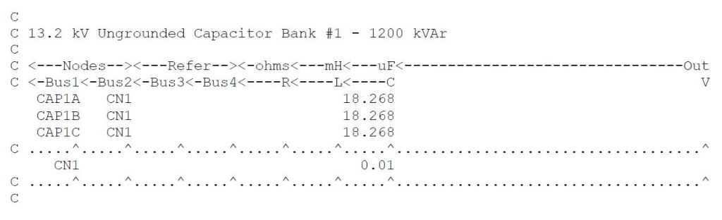
One commonly used method for the creation of EMTP data files deals with use of “template” files. These files provide the necessary formatting and allow the user to concentrate on the data preparation. An example of template style data is illustrated below.
Program Outputs
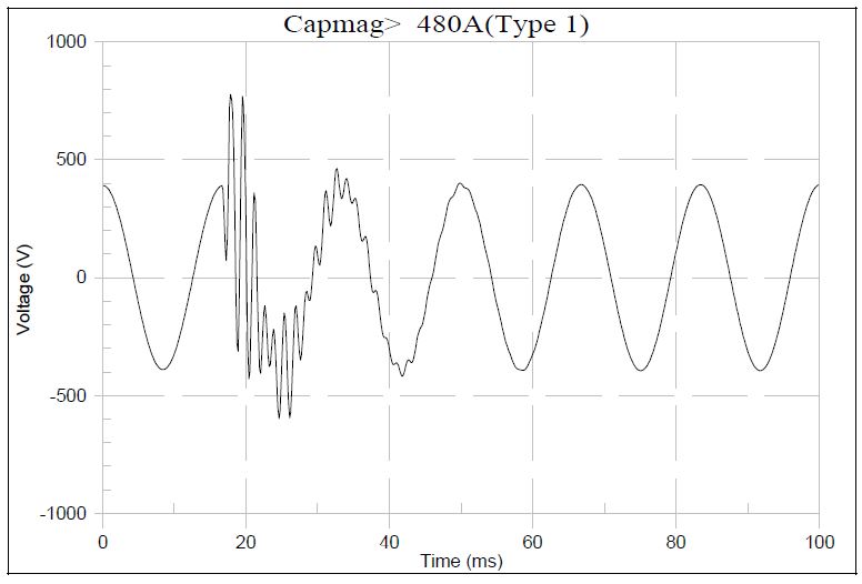
The main output of an EMTP simulation consists of the magnitude vs. time points for node voltages (illustrated in Figure 1), differential voltages (node–node), and branch currents. Other outputs from the transient case can also be calculated by EMTP (energy, power, etc.) but it is generally easier to let the output processing program generate these supplemental signals from the actual voltage and current data.
The program performs a full steady state solution to develop initial conditions for the linear elements in the model. The initial conditions used for nonlinear elements depend on the specific model involved. The output from the steady state solution is also available in different levels of detail and can be very useful for debugging the model.
The various output quantities available include:
− Steady-state phasor solution – branch voltages and currents, bus voltages, power loss, and power flows
− Data points for bus voltages, branch voltages, branch currents, branch energy dissipation, machine variables, and control system variables
− Voltage magnitudes and angles as a function of frequency (frequency scan option)
− Statistical summary data for statistical cases
Study Procedure
The following is a suggested procedure for using EMTP to perform distribution system transient studies:
− Identify Study Objectives. The objectives will dictate the frequency range of interest, the modeling requirements, the variables to be investigated, and the types of output that are needed from the simulation.
− Determine Frequency Range of Interest. The frequency range will determine the type of component models required for the study, the required time step size, and the duration of the simulation. Some guidelines for determining the frequency range of interest and the impact on the required component models are provided in the Modeling Guidelines section of this report.
− Develop System Model. The extent of the system model depends on the capacitors and/or lines to be switched and the frequency range of interest. Obviously, it would be desirable for the model to include the entire system so you could just switch the device(s) of interest. However, the solution times for a very large model becomes excessive, and there is often limited improvement in accuracy beyond a more reduced model around the circuit of interest.
− Draw Connection Diagram and Label Buses. The bus labels will be used in the EMTP data file for identification.
− Develop Component Models. Each component model (transmission line, distribution feeder, transformer, capacitor, breaker, etc.) will depend on the frequency range of interest and the specific transient event being evaluated.
− Run a Steady State Solution Case. This case will verify system connectivity and provides a sanity check for many of the system components.
− Estimate Expected Results. This can be done from previous studies, from the literature, or from hand calculations. It is important to know what to expect from the simulation so that major problems can be identified quickly.
− Sensitivity Analysis for Important Variables. Important variables from the simulation should be evaluated to determine their impact on results. These could include breaker closing instants, transformer saturation, line length, capacitor size, etc.
− Develop Solutions. Possible solutions (i.e. pre-insertion resistors) are evaluated and design specifications are developed.
Simulation Process
The process for completing a transient simulation (shown in Figure 2) consists of first collecting and developing the necessary data to represent the circuit to be modeled. Often this system representation is completed by “describing” the interconnection and component values in a simple ASCII text file. This text file method is a hold-over from earlier times, when the data was read line-by-line with a card reader. After the data file (.DAT) has been created, it is submitted to the EMTP solver. The solver reads the data file, line-by-line, and reports any significant errors (to be discussed in greater detail in an upcoming section). Satisfied that the case will solve the EMTP generates a matrix representation of the interconnected system. Typically, solution of both a steady-state case and a transient case occur.
There are two forms of EMTP output available for viewing. First, an ASCII text output (.OUT) file is produced. This file contains a summary of how the EMTP interpreted the input data file (useful for debugging component values), a connectivity table, full output of the steady-state case, and the requested output for the transient case. This transient output is also stored in a binary file (.PL4) for post processing and viewing.

Developing a System Model
One of the most important problems associated with developing a system model is: “How much of the system do I need to model?” Unfortunately, there are no rules to guide a user, it is often more of a feel that is developed over time. A good starting point for switching studies is to model one or two buses back from the switched bus. However, even this simple guideline fails from time-to-time. Perhaps the best method for determining the appropriate system model is to start with a small simple circuit that accurately represents the phenomena, and then add more of the system details to determine their impact on the solution result. Another factor in the system modeling question is model/simulation accuracy. Very often the goal of the study will determine the model complexity:
Selection of the time step is one of the most important decisions an EMTP user must make. Improper time step selection is analogous to selecting a monitoring device that samples a waveform at a slow enough rate that the transient of interest is partially or completely missed. There needs to be a balance between computational effort and accuracy when the time step is selected. The selection, much like the modeling question, is more of a feel then a hard and fast rule.
Frequency Ranges for EMTP Simulations
The study of electrical transient phenomena involves a frequency range from DC to about 60 MHz. Typically, electromagnetic phenomena involves frequencies above the power frequency, and electromechanical phenomena involves frequencies below the power frequency. Transient phenomena appear as transitions from one steady-state condition to another. The primary causes of these transitions are switching operations and lightning. Generally, the frequency of the resulting disturbance will fall somewhere in the following range (Table 1):
Table 1 – Frequency Range for Power System Transients
Model Verification
The single most important tool that the user has for verifying the EMTP case results is a basic knowledge of power system transients. Field test results, technical papers, basic textbooks, and more experienced engineers can all help. The textbook by Allan Greenwood, Electrical Transients in Power Systems, is a useful reference and it is recommended that the user review the basics of the phenomena before attempting to simulate it with the EMTP. Learning by doing can be very frustrating and applying the simulation results can be risky, when the user does not feel comfortable with the results of the study.
When verifying the results of an EMTP case, the user should always check the input parameter interpretation and network connectivity table. The steady-state solution should be checked to verify known quantities, such as bus voltage, branch currents, etc.
Pre-switching steady-state waveforms should be examined for characteristic harmonic content and the waveform should be allowed to reach a stable condition before any switching is done.
An example of this is the interaction between capacitor switching and adjustable-speed drives (ASDs). There are actually two transients events that occur during the simulation, however it only the second event – capacitor switching – that is of any interest. The first event, ASD starting, should be allowed sufficient time to reach a stable operating point before the capacitor is switched. There are a number of methods for accomplishing this task, however, at times the easiest method is to simply let the simulation run long enough to stabilize.
Evaluation and Presentation of Results
Upon completion of the transient simulation case, an evaluation of the accuracy of the results is required. As previously mentioned, it is desirable that the user have a basic understanding of the phenomena of interest. In essence, the user should know what the result should be (or at least a good idea of what the waveform should look like) before completing the case. In reality, however, this is not always the case, so it becomes even more important that the user have confidence in the accuracy of the data file.
Simulation results are generally presented in the form of overvoltage and overcurrent quantities. Overvoltages are generally quantified in per-unit of the maximum crest (peak) line-to-ground voltage. This applies for both line-to-line and line-to-ground transient voltages.
Presentation of simulation results may take a number of different forms (i.e. graphical, tabular, etc.). It may be just as important to present the result in a way easily understood by the audience, as it is to complete the simulation correctly. Failure of either results in no action taken.
The main output of an EMTP simulation consists of the magnitude vs. time points for node voltages (previously illustrated in Figure 1), differential voltages (node-node), and branch currents. Other outputs from the transient case can also be calculated by EMTP (energy, power, etc.) but it is generally easier to let the output processing program generate these supplemental signals from the actual voltage and current data. The various output quantities available include:
− Steady-state phasor solution – branch voltages and currents, bus voltages, power loss, and power flows
− Data points for bus voltages, branch voltages, branch currents, branch energy dissipation, machine variables, and control system variables
− Voltage magnitudes and angles as a function of frequency (frequency scan option)
− Statistical summary data for statistical cases
In addition, study results may take the form of summary tables and/or graphs that illustrate the results for multiple simulations. For example, one common method for presentation of results is in the form of an overvoltage vs. variable graph. The “variable” may be quantities like line length, transformer size, capacitor size, choke size, etc. It is much easier for the audience to understand the impact of a specific variable on the overvoltage range using this method (as opposed to page after page of simulation waveforms).
REFERENCES
Electrical Transients in Power Systems, Second Edition, A. N. Greenwood, John Wiley and Sons, New York, 1991.
Electromagnetic Transients Program (EMTP) Rule Book, Version 2.0, vol. 1, vol. 2, EPRI EL-6421-L, Electric Power Research Institute/DCG, June 1989.
Electromagnetic Transients Program (EMTP) Revised Application Guide, Version 2.0, EPRI EL-7321, Electric Power Research Institute /DCG, November 1991.
Electromagnetic Transients Program (EMTP) Primer, EPRI EL-4202, Project 2149-1, Electric Power Research Institute, September 1985
GLOSSARY AND ACRONYMS
ASD: Adjustable-Speed Drive
CT: Current Transformer
EMTP: Electromagnetic Transients Program
HVAC: High-Voltage Air Conditioning
MOV: Metal Oxide Varistor
PF: Power Factor
PWM: Pulse Width Modulation
TVSS: Transient Voltage Surge Suppressors
