Published by Electrotek Concepts, Inc., PQSoft Case Study: Modeling Ferroresonance in an Underground Distribution System, Document ID: PQS0610, Date: July 1, 2006.
Abstract: The objective of this case study is to provide an overview of ferroresonance phenomena, its modeling aspects, and practical experience in recognizing, avoiding, and solving the problem. In particular, it will present symptoms of ferroresonance. An actual example simulation analysis involving an underground cable circuit with blown fuses is presented along with solutions to avoid ferroresonance.
INTRODUCTION
Ferroresonance is a general term applied to a wide variety of resonance interactions involving capacitors and saturable iron-core inductor. During the resonance the capacitive and inductive reactances are equal with opposite values, thus the current is only limited by the system resistance resulting in unusually high voltages and/or currents. Ferroresonance in transformers are more common than any other power equipment since their cores are made of saturable ferrous materials.
Ferroresonant overvoltages on distribution systems were observed early in the history of power systems (i.e., early 1900s). In this case study, the theory of ferroresonance is briefly presented. More theoretical description can be found in documents listed in the reference section. Symptoms of ferroresonance and personal accounts of engineers who witnessed the phenomena are provided. Ferroresonant modeling and a case study of an actual ferroresonance problem with its corresponding solutions is also included in the case.
PRINCIPLES OF FERRORESONANCE
There are various ways to understand ferroresonance. One method is to begin with a review of a simple RLC circuit. Figure 1 shows a voltage source with an arbitrary frequency, such as 50 Hz or 60 Hz.
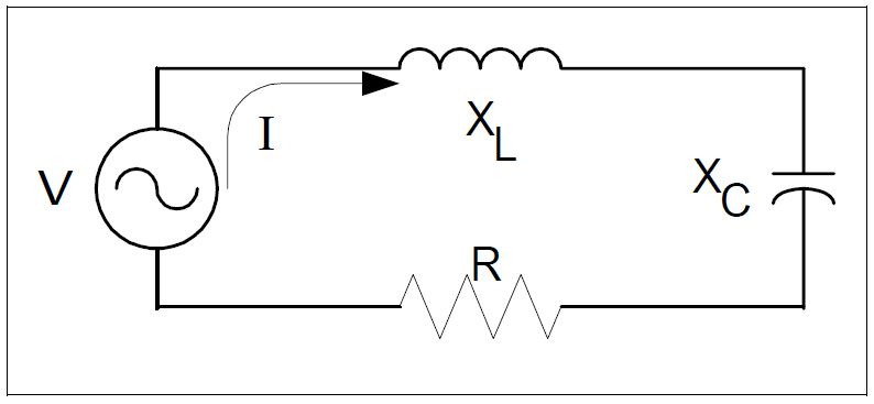
The inductive (XL) and capacitive (XC) reactances are assumed to be constant or linear. Furthermore, it is assumed that the resistance (R) is much smaller than |XL| and |XC|. The magnitude of current flowing in the circuit is approximately:
I = V / R + XL – XC ≅ V / XL – XC
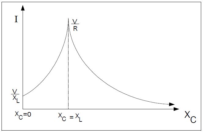
Let us vary XC and hold R and XL at a constant value. When XC = 0, the current flowing in the circuit is I=V/ XL, and when XC is very large, the current becomes negligible. In between these two extremes, |XC|=|XL|. The current becomes very large limited only by R, i.e., I=V/ R. The large current can produce considerable overvoltage. Figure 2 illustrates the magnitude of current under various XC values. The possibility of XC exactly matching XL is remote since both values are linear or constant. However, if the value of XL varies, such as in an iron core transformer, the possibility of XC equaling XL increases considerably.
Alternatively, the solution to the above circuit can be written as follows:
VL = jXLI = V – (-jXC)I or, v = XLI, and v = V – XCI
where V is an arbitrary voltage.
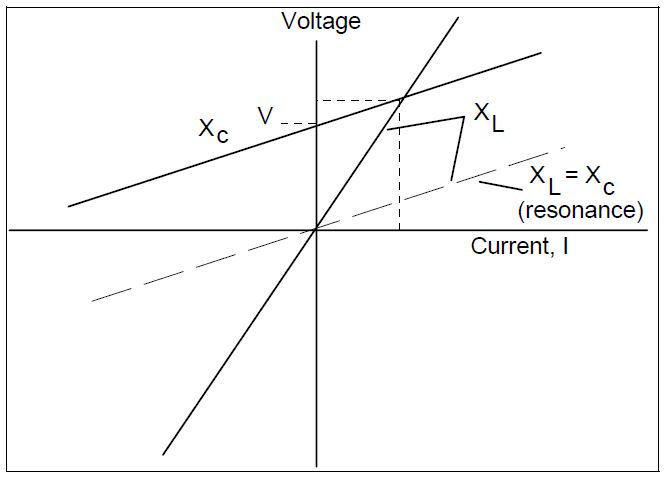
The intersection between the inductive reactance XL line and the capacitive reactance XC line yields the current in the circuit and the voltage across the inductor, VL. The above solution is depicted in Figure 3. At resonance, these two lines become parallel, yielding solutions of infinite voltage and current (assuming lossless element).
When XL is no longer linear, such as a saturable inductor, the XL reactance can no longer be represented with a straight line. The graphical solution is now as shown in Figure 4.
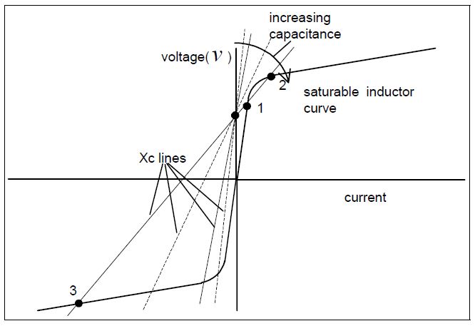
It is obvious that there may be as many as three intersections of the capacitive reactance line with the inductive reactance curve. Intersection 2 is an unstable operating point and the solution will not remain there in steady-state. However, it may pass through this point during a transient. Intersections 1 and 3 are stable and will exist in steady-state. Obviously, if the values become an intersection 3 solution, there will be both high voltages and high currents. For small capacitances, the XC line is very steep, usually resulting in only one intersection in the third quadrant. The capacitive reactance is larger than the inductive reactance, resulting in a leading current and higher than normal voltages across the capacitor. The voltage across the capacitor is the length of the line from the system voltage intersection to the intersection with the inductor curve. As the capacitance increases, there can be multiple intersections as shown. The natural tendency then is to achieve a solution at intersection 1, which is an inductive solution with lagging current and little voltage across the capacitor. Note that the voltage across the capacitor will be the line-to-ground voltage on the cable in a typical power system ferroresonance case.
If there is a slight increase in the voltage, the capacitor line would shift upward, eliminating the solution at intersection 1. The solution would then try to jump to the third quadrant. Of course, the resulting current might be so large that the voltage drops again and the solution point jumps between 1 and 3. Indeed, phenomena like this are observed during instances of ferroresonance. The voltage and current appear to vary randomly and unpredictably.
In the usual power system case, ferroresonance occurs when a transformer becomes isolated on a cable section in such a manner that the cable capacitance appears to be in series with the magnetizing characteristic of the transformer. For short lengths of cable, the capacitance is very small and there is one solution in the third quadrant at relatively low voltage levels. As the capacitance increases the solution point creeps up the saturation curve in the third quadrant until the voltage across the capacitor is well above normal. These operating points may be relatively stable, depending on the nature of the transient events that precipitated the ferroresonance.
SYMPTOMS OF FERRORESONANCE
There are several modes of ferroresonance with varying physical and electrical characteristics. Some have very high voltages and currents while others have voltages close to normal. In this section symptoms of ferroresonance are presented.
Audible Noise
One thing common to all types of ferroresonance is that the steel core is driven into saturation, often deeply and randomly (otherwise, it is conventional resonance and not considered ferroresonance). As the core goes into a high flux density, it will make an audible noise due to the magnetostriction of the steel and to the actual movement of the core laminations. In ferroresonance, this noise is often likened to shaking a bucket of bolts, whining, or to a chorus of a thousand hammers pounding on the transformer from within. In any case, the sound is distinctively different and louder than the normal hum of a transformer.
Overheating
Another reported symptom of the high magnetic field is due to stray flux heating in parts of the transformer where magnetic flux is not expected. Since the core is saturated repeatedly, the magnetic flux will find its way into the tank wall and other metallic parts. One possible side effect is the charring or bubbling of paint on the top of the tank. This is not necessarily an indication that the unit is damaged, but damage can occur in this situation if the ferroresonance has persisted sufficiently long to cause overheating of some of the larger internal connections. This may in turn damage insulation structures beyond repair.
Arrester and Surge Protector Failure
The arrester failures are related to heating of the arrester block. One common failure scenario is for line personnel to discover an open fused cutout and to simply replace the fuse. Meanwhile, the arrester on that phase has become very hot and goes into thermal runaway upon restoration of full power to that phase. Failures are often catastrophic with parts being expelled from the arrester housing. Under-oil arresters are less susceptible to this problem because they are able to dissipate the heat due to the ferroresonance current more rapidly.
Flicker
Customers are frequently subjected to a wavering voltage magnitude. Light bulbs will flicker between very bright and dim. Some electronic appliances are reportedly very susceptible to the voltages that result from some types of ferroresonance, but we have no knowledge of the alleged failure mode. Perhaps, it is simply MOV failure in the power front end. These frequently fail catastrophically, going into thermal runaway and then burning open with considerable arcing display. This may do nothing more than pop a breaker, but surge protection is lost for any subsequent surge that might damage the appliance.
Cable Switching
The transformers themselves can usually withstand the overvoltages without failing. Of course, they would not be expected to endure this stress repeatedly because the forces often shake things loose inside and abrade insulation structures. The cable is also in little danger unless its insulation stress had been reduced by aging or physical damage. Of course, operating a solid dielectric system above its normal stress level for an extended period can be expected to create some shortage of life.
It may be difficult to clear arcs when pulling cable elbows if ferroresonance is in progress. The currents may be much higher than expected and the peak voltages may be high enough to cause reignition of the arc.
Some utilities will not perform cable switching involving three-phase padmount transformers without first verifying that there is substantial load on the transformers. One of the common solutions to ferroresonance during cable switching is to always pull the elbows and energize the unit at the primary terminals. This will normally work because there is no external cable capacitance to cause ferroresonance. There is little internal capacitance, and the losses of the transformers are usually sufficient to prevent resonance with this small capacitance. Unfortunately, modern transformers are changing the old rules of thumb. The newer low-loss transformers, particularly, those with amorphous metal core, are prone to ferroresonance.
TRANSFORMER MODELING
Ferroresonance can be mysterious subject. Probably the main reason is that the analysis requires sophisticated nonlinear circuit analysis techniques. The results are sometimes unpredictable and certainly difficult to visualize (unlike linear circuit phenomena). Another issue that complicates the analysis of ferroresonance is that there are several different types of three-phase transformers such as three single-phase transformers connected as a three-phase transformer, three-legged core transformers, three-phase shell-type transformers, four-legged core, and five-legged cores. The conventional T model of a two-winding transformer, and the five-legged core transformer model will be summarized in this section.
For single-phase transformers, three-phase shell form transformers, and three-phase triplexed transformers (three single-phase units stacked in one can), the conventional T model will suffice because there is no coupling between the magnetic circuits. Figure 5 shows the T model for a two winding transformer, which will suffice for standard switching surge and ferroresonance studies. For higher frequencies, it would be necessary to model the capacitances and inner winding construction.
The terminals of this model can be connected to represent any two-winding transformer with magnetically independent phases. The saturable inductance data are readily available from the manufacturer’s test data. Note that manufacturers supply the rms v-i curve. This must be converted to a peak flux-current curve before it can be used in EMTP or other transients programs. This conversion is a bit tricky because the current waveforms are not sinusoidal. Therefore, one cannot simply multiply the current values on the rms curve by 1.414 to determine the correct peak value. The usual procedure is to use a computer program that reconstructs the peak saturation curve by iterative solution. The first point can be established by multiplying by 1.414. Then a guess is made at the next point and the waveform is reconstructed. The guess is adjusted until the rms of the reconstructed waveform matches that supplied by the manufacturer.
The five-legged core transformer design [3] is illustrated in Figure 6. The design typically consists of four individual cores tied together to create the five-legged core transformer. The inner three legs carry the phase windings with flux paths as indicated. The equivalent circuit can be derived from the flux path direction and is shown in Figure 7.
CASE STUDY
In this section, an actual case study is presented. A ferroresonance condition developed on an approximately 5,000-foot underground cable feed to a medical facility. When one of the riser pole fuses blew, severe voltage fluctuations occurred at the load. As a temporary solution the utility replaced the fuses with a three-phase recloser and wanted to see under what conditions the three-phase recloser might be removed and the fuses reinstalled. Therefore, the purpose of this case study was to determine under what conditions the ferroresonance at the underground distribution network could be avoided (and whether fuses might be reinstalled instead of keeping the three-phase recloser).
The ferroresonance condition apparently did not cause damages to the two 500 kVA transformers nor the customer loads at the medical facility. However, it was reported that a sudden overvoltage did occur and lights flickered between bright and dim.
A simplified one-line diagram to study the ferroresonance problem is shown in Figure 8. The simulation model was developed using the EMTP program.

The lengths of the cable from the first pole to the first switch (S1), and from the first switch (S1) to the second switch (S2) were approximately 1,900 feet and 2,150 feet long. The cable size was 600 MCM with the following characteristics:
Insulation: 0.1406 outside diameter in feet
Jacket: 0.1412 outside diameter in feet
Neutral: 0.1409 outside diameter in feet
A line constant program was used to compute the positive and zero-sequence impedances of the cable, yielding the following results:
z1 = 0.0231 + j 0.0824 ohm/1000ft
z0 = 0.1828 + j 0.6854 ohm/1000ft
C1 = C0 = 78.24 nF/1000 ft.
The lengths of the underground cable from the second switch (S2) to the first transformer (JL61), and from the first transformer (JL61) to the second transformer (KL30) were 420 and 450 feet long, respectively. The type of the cable was 1/0 with the following characteristics:
Insulation: 0.0629 outside diameter in feet
Jacket: 0.0688 outside diameter in feet
Neutral: 0.0794 outside diameter in feet
The computed positive and zero-sequence impedances were:
z1 = 0.0803 + j 0.0952 ohm/1000ft
z0 = 0.4061 + j 0.5150 ohm/1000ft
C1 = C0 = 97.34 nF/1000 ft
The two 500 kVA transformers were modeled according to the five-legged core transformer design. In order to investigate overvoltage due to ferroresonance, one phase of the cable was intentionally opened to simulate circumstances leading to ferroresonance (e.g., fuse blows, cable connector or splice opening, etc.). In the simulation, phase B at the first pole was open-circuited, while switches S1 and S2 shown in Figure 8 were closed at all times. Resistive loads at the secondary winding of transformers JL61 and KL30 were increased from zero to 30% of the transformer capacities, i.e., from 0 to 150 kW.
Figure 9 shows voltage waveforms at the secondary winding of transformer JL61 when both JL61 and KL30 transformers are unloaded. Since the voltage at the secondary of transformer KL30 is nearly identical to that of JL61, the voltage waveforms are not shown. Industry analysts have historically assumed that when the voltage exceeds 1.25 per-unit, the system is said to be “in ferroresonance”. Figure 9 clearly illustrates that the system is in ferroresonance condition since phase B exhibits sustained overvoltage approaches 3.0 per-unit.
Figure 10 (top left) shows the voltage waveforms at the secondary winding of JL61 transformer when both JL61 and KL30 transformers are loaded with resistive load equivalent to 5% of transformer capacities. In other words, JL61 and KL30 transformers are loaded with 25 kW loads. The overvoltage at phase B is now approximately 2 per-unit, much less compare to when both transformers are unloaded.
In the similar fashion, loads at both transformers are added successively, i.e., 10, 15, 20, 25, and 30% of the transformer capacities. As loads increase the overvoltage drops quickly. Figure 10 shows the voltage waveforms at the secondary winding of transformer JL61 when both transformers are loaded with 5% (top left), 15% (top right), 20% (bottom left), and 30% (bottom right) of their respective capacities.
With 15% of load, the system remains in ferroresonance condition since it exhibits sustained overvoltage of 1.5 per-unit. The ferroresonance condition is practically eliminated when both transformers are loaded with 20% of resistive load. The overvoltage magnitude is about 1.4 per-unit at when phase B is open, however this overvoltage is not sustained and quickly decays to a low voltage. With 30% of load, the system is not in ferroresonance either. Twenty percent of resistive load is sufficient to avoid the ferroresonance condition.
(with (a) 5%, (b) 15%, (c) 20%, and (d) 30% of their Respective Capacities)
Figure 11 shows the summary of peak overvoltages when both transformers are loaded from 0% to 30% of their capacities. The overvoltage on phase B drops quickly as both transformers become more loaded. From the analysis presented in this section, it can be concluded that both transformers should be loaded with a minimum of 100 kW resistive load or loads equivalent to 20% of transformer capacity to avoid the ferroresonance condition. The rapid drop in ferroresonant voltage magnitude is due in large part to the introduction of the resistive load.
Based on the study, the ferroresonance condition can be avoided by having both transformers loaded with at least 20 percent of their respective capacities. In other words, each transformer must have 100 kW (resistive) at its secondary winding. When one phase is open-circuit, there will be a momentary overvoltage as high as 1.4 per-unit, however it quickly decays to a low voltage. There will be no sustained ferroresonance overvoltage. If this minimum loading can be guaranteed, it is safe to replace a three-phase recloser with three fuses.
In the event that the loading cannot be achieved, it is advised to use the three-phase switchgear to avoid the ferroresonance condition. The minimum load of 20% to avoid ferroresonance is much higher than the usual minimum load of 5%. The higher minimum is primarily due to the length of the cable involved, which is approximately 1 mile long.
SUMMARY
A fundamental description of ferroresonance has been presented in this case study. In particular, analysis of the ferroresonance condition based on a simple graphical approach is presented. Several transformer models are also included for reference. Finally, a representative case study showing ferroresonance in an underground cable circuit is included. Minimum load levels for mitigating ferroresonance are evaluated.
REFERENCES
[1] R. Rudenberg, Transient Performance of Electric Power Systems, New York, NY, McGraw-Hill Company, 1950.
[2] C. Hayashi, Nonlinear Oscillations in Physical Systems, New York, NY, McGraw-Hill Company, 1964.
[3] D. L. Stuehm, B. A. Mork, D. D. Mairs, “Five-legged core transformer equivalent circuit”, IEEE Transactions on Power Delivery, Vol 4, No. 3, July 1989, pp. 1786.
[4] Slow Transient Task Force of the IEEE Working Group on Modeling and Analysis of System Transients Using Digital Programs, “Modeling and analysis guidlines for slow transients – Part III: The study of ferroresonance,” IEEE Trans. on Power Delivery, vol. 15, No. 1., Jan. 2000, pp. 255 – 265.
RELATED STANDARDS
IEEE Std. C57.105-1978
GLOSSARY AND ACRONYMS
MOV: Metal Oxide Varistor Arrester
MSSPL: Maximum Switching Surge Protective Level
SiC: Silicon Carbide Arrester
