EMC for 2 to 150 kHz: A Proposal for Emission and Immunity of Equipment including Power-Line Communication

Published by Anders Larsson and Math Bollen, ELFORSK, Elforsk rapport 09:29, October 2008

Summary

The frequency range from 2 to 150 kHz is not sufficiently covered in international standards. The contrast with the frequency range below 2 kHz is striking. There have traditionally been good reasons to emphasize on the lower frequency range, where the absence of mitigation measures would lead to serious problems.

For frequencies above 150 kHz, potential interference with public radio broadcasting has been the driving force for standardization.

In the frequency range 2 – 150 kHz no significant sources of emission used to exist. Also no widespread problems due to high disturbance levels in this range have been reported yet.

There are however two good reasons for turning the attention to this frequency range. The first is the use of (part of) this frequency range for power-line communication. The second is the increasing use of end-user equipment emitting conducted disturbances in this frequency range.

Based on the measurement of voltage and current distortion, three types of disturbances are recognized in the frequency range 2 to 150 kHz.

Narrowband signals appear mainly in the form of individual frequencies due to power-line communication.
Broadband signals are mainly due to individual end-user equipment with active power-factor correction.
Recurrent oscillations (typically every 10 ms) are due to limitations of the power-electronic converters around the current zero crossing.

For each of these disturbance types, compatibility levels, emission limits and immunity limits are needed to come to a working EMC framework. Proposals are made for narrowband and broadband signals. No proposal has been made for recurrent oscillations due to the lack of information available at the moment.

When power-line communication is used, some measured are needed against low impedance of non-communication equipment. This may be measures taken by the operator of the communication equipment on a case-by-case basis or requirements on the minimum input impedance of equipment in the frequency range used for power-line communication.

We propose to use the time domain for measurements throughout the frequency band 2 to 150 kHz.

1 Introduction

For frequencies above 150 kHz, potential interference with public radio broadcasting has been the driving force for standardization.

In the frequency range 2 – 150 kHz no significant sources of emission used to exist. Also no widespread problems due to high disturbance levels in this range have been reported yet.

This document will give an overview of the existing standards in this frequency range and propose additional standardization towards a more complete set of standards. The proposals are based on a range of measurements of voltage and current disturbances in this frequency range.

2 The IEC concept of electromagnetic compatibility

The concept used in IEC for achieving electromagnetic compatibility in a system, including some of the terminology used, is shown schematically in Figure 2.1. A similar figure is shown in Annex A of IEC 61000-2-2 and in several other publications.

Figure 2.1, The IEC concept of electromagnetic compatibility.

The figure specifies a number of different levels and limits, which will be discussed briefly below¹.

2.1 Compatibility level

The compatibility level is a reference level for coordinating emission limits and immunity limits. The term was originally introduced for radiated emission with one emitter and one suscepter. The compatibility limit would in that case be chosen as an economic balance between reducing emission and improving immunity.

¹ For a detailed discussion of the various terms and existing standards, see: Math Bollen – Problembeskrivning och emission och immunitet, STRI rapport R08-470, February 2008. This report will also be available as an Elforsk report.

For equipment connected to the power system the situation is more complex. The electromagnetic environment to which a device is exposed is due to the emission of several to many individual devices and is also influenced by the way in which the disturbances propagate through the power system. For conducted disturbances the compatibility level has often been coordinated with the existing disturbance levels in the power system. Emission limits for individual sources are set in such a way that the disturbance levels do not exceed the compatibility levels.

2.2 Planning level

Planning levels are used by a network operator to prevent the disturbance levels from exceeding the electromagnetic compatibility levels² or any levels set by a regulator. The choice of planning levels is up to the network operator, but they should obviously not exceed the levels set by the regulator. The planning levels are used among others to determine the need for additional mitigation measured when connecting new loads. The planning levels. being internal quality objectives used by the network operator, are not set by IEC, but IEC does give indicative planning levels for some disturbances at different voltage levels (harmonics and voltage fluctuations at MV level and higher).

² One may argue that compatibility levels do not concern the network operator, but that planning levels instead should be compared with voltage characteristics. This discussion is out of the scope of this report.

2.3 Emission limit

According to e.g. IEC/TR 61000-3-6 is “emission limit” defined as the “maximum emission level specified for a particular device, equipment, system or disturbing installation as a whole, assessed and measured in a specified manner”. The latter part of the phrase (assesses and measured in a specified manner) is very important and the cause for many discussions and misunderstandings, within standard-setting groups as well as for those using the standards.

The equipment standards set a limit on the emission of a device, under strictly defined and controlled laboratory conditions. The reason for this is the need for being able to reproduce the results: the testing result should be the same for different testing labs.

A consequence of this is however that the emission in reality, i.e. when connected to a power system with many other devices connected, will be different and that it may exceed the emission limit. This is one of the reasons for the spread of “emission level of the system” in Figure 2.1. The intention of the emission tests is however that a device with an emission below the limit during the test will not cause emission widely exceeding the limit in reality. In other words: passing the test should be a guarantee for limited emission during practical use. Note that this is a guarantee mainly towards the network operator. Under the EMC directive, the manufacturer and user of the equipment are no longer responsible once the equipment has passed the required tests.

The emission limit sets the maximum disturbance level generated by equipment, often measured at the mains terminal of the equipment. These limits are normally set for a single source and one piece of equipment. The emission levels can be measured as a current or as a voltage against a standardized source impedance.

For harmonics in the frequency range up to 2 kHz, IEC 61000-3-2 sets limits for the current emission for each harmonic frequency. But for fast fluctuations in load current, the emission limit is set as a maximum Pst value against a reference impedance.

2.4 Immunity limit

This is defined in e.g. IEC/TR 61000-3-6 as, ”the maximum level of a given electromagnetic disturbance on a particular device, equipment or system for which it remains capable of operating with a declared degree of performance”.

The same restrictions hold for the immunity limit as for the emission limit discussed before: it holds only under well-defined laboratory conditions. A number of disturbances are defined in detail and the device is exposed to those. The underlying assumption is that if a device is immune to these “standard disturbances”, it will be able to cope with the majority of disturbances that occur in reality. It will be clear that this is not always the case and the discussion on this is ongoing both within standard-setting groups and within the wider power-quality community.

To make sure that the equipment can operate when connected to the grid together with other loads it is subjected to different test. Some typical tests could be dips, transients, voltage fluctuations, magnetic fields etc. For example, tests against harmonic voltage distortion are prescribed in IEC 61000-4-13.

3 Disturbances in the frequency range 2 to 150 kHz

Measurements have been performed of the voltage distortion to which equipment is exposed in the frequency range from 2 to 150 kHz. The results of these measurements are presented among others in [5][6][7]. This work and other publications have resulted in the following subdivision of disturbances occurring in this frequency range:

Narrowband signals;
Broadband signals;
Recurring oscillations.

These three types of disturbances will be described separately below. For each of these three types, emission, compatibility and immunity levels should be defined. The setting of these levels will be discussed in Chapters 4, 5 and 6.

Based on the compatibility levels, voltage characteristics and planning levels can next be chosen.

3.1 Narrowband signals

Narrowband signals appear mainly in the form of individual frequencies due to power-line communication. Also individual equipment may emit narrowband signals, but the resulting levels of voltage distortion remain well below the voltage signals used for power-line communication. Existing standards define the maximum emission levels for communication equipment in this frequency range. The compatibility level should be above this emission level. The immunity level of both communication and non-communication equipment should in its turn be above the compatibility level. This will be discussed further in Chapter 5.

3.2 Broadband signals

Broadband signals in the frequency range 2 to 150 kHz are mainly due to individual end-user equipment with active power-factor correction. Also expected future equipment like solar panels, microgeneration and chargers for hybrid-electric cars will most likely emit this kind of signals. The distortion is related to the switching frequency used in the power-electronic converters. The switching frequency however varies with time and is different for different devices so that the resulting voltage distortion has in many cases a broadband character.

It was shown that the emission of active power-factor correction circuits shows a complex time-frequency behaviour. However the resulting voltage distortion, being caused by the sum of many individual devices, has more of a broadband character even in time-frequency domain.

An example of emission due to a broadband signal is shown in Figure 3.1. The corresponding spectrum is shown in Figure 3.2. The oscillations that are visible in the time domain around the current maximum and minimum show up as a band in frequency from about 40 to 80 kHz.

Figure 3.1. Example of broadband signals: currents measured in a lighting installation; measured waveform (top) and high-pass filtered waveform (bottom).

Figure 3.2. Spectrum of the current shown in Figure 3.1, grouped into 200-Hz bands.

To analyse the sub-cycle variations in distortion neither the frequency domain nor the time domain is a suitable tool. Instead the time-frequency domain spectrogram has been proposed and successfully used for this [5][6][7]. Using a time-frequency description (like in the spectrogram) would introduce unnecessary complications for standardization purposes. The time-frequency domain remains a useful tool however for analysis of waveform distortion in the frequency range from 2 to 150 kHz.

By extrapolation of the requirements for harmonic voltage distortion just below 2 kHz, a safe level equal to 0.5% (of nominal voltage) per 200-Hz band has been concluded in [1] as a planning level. A compatibility level equal to or somewhat above this level could be appropriate. The immunity level should be chosen above the compatibility level.

Any emission levels should be chosen such that the resulting voltage distortion will not exceed the compatibility level for practical source impedances and number of devices. This will be discussed further in Chapter 6.

3.3 Recurring oscillations

These are for example due to limitations of the power-electronic converters resulting in oscillations around every voltage zero crossing. The frequency of these oscillations is a few kHz, amplitudes up to 20 Volt have been observed and they repeat every 10 milliseconds.

A measurement of recurrent oscillations is shown in Figure 3.3. The measurement was performed near a group of fluorescent lamps in a shop. The low-frequency components, including the power-system frequency, have been removed by means of an analog filter with a cut-off frequency of 2 kHz. The three traces correspond to the three phases. Oscillations are visible (in the form of spikes) in two of the three phases recurring every 10 ms. The oscillations are either absent or lost in the broadband signal in the third phase.

Figure 3.3. Measured high-pass filtered voltage in three different phases.

Measurements at many locations have shown that such recurrent oscillations are a common phenomenon. Their origin is shown in Figure 3.4: the current drawn by a fluorescent lamp with high-frequency ballast as measured in the Pehr Högström laboratory at Luleå University of Technology. The top trace shows the measured current, the bottom trace shows the high-pass filtered version. A digital filter with a cut-off frequency of 2 kHz has been used. The notches present in the non-filtered current are associated with oscillations when the current restarts. The presence of these notches is referred to in the power-electronics literature as “zero-crossing distortion” or “cross-over distortion”, hence the term “zero-crossing oscillations” to refer to these recurrent oscillations.

Figure 3.4. The current drawn by one fluorescent lamp (top) and the digital band-pass filtered version (bottom).

The reason for the importance of these recurrent oscillations is shown in Figure 3.5. The timing of the oscillations are linked to the zero-crossing of the current which in turn is linked to the zero-crossing of the voltage. As all equipment experiences the same voltage, the oscillations occur at the same time for all equipment. The result is that the magnitude of the oscillations increases with increasing number of devices. This is illustrated in Figure 3.5 showing measurements done in the Pehr Högström laboratory. The three traces show the current taken by one, three or nine fluorescent lamps. The increase in magnitude of the recurrent oscillations is obvious.

Figure 3.5. Filtered current with one (top), three (middle) and nine (bottom) lamps connected.

These recurrent oscillations form a new type of disturbance, for which neither characteristics, not limits exist. This will make it difficult to set standards. This will be discussed further in Chapter 6.

4 Narrowband signals

4.1 Existing limits

Maximum emission due to power-line communication is given in the form of voltage limits in EN 50065-1 and in IEC 61000-3-8. According to these standards is the signal considered as a narrow band signal if its bandwidth is less than 5 kHz. Voltage characteristics are given in EN 50160, where they are referred to “voltage levels of signal frequencies”.

The emission limits according to EN 50065 and IEC 61000-3-8 are reproduced in Figure 4.1. The two vertical lines indicate the frequency range of interest for this document (2 to 150 kHz). Note that the emission limits are expressed in terms of voltage. There is no reference impedance associated with this limit; the voltage after injection of the communication signal shall not exceed the indicated limit. For frequencies up to 95 kHz the limits are the same for both standards. EN 50065 does not cover frequencies above 150 kHz. IEC 61000-3-8 does give limits but these are an order of magnitude more restrictive than below 150 kHz. This is to prevent interference with commercial broadcasting (the long-wave band starts at 150 kHz).

Figure 4.1. Emission limits for narrowband signals according to EN 50065 (blue solid line) and IEC 61000-3-8 (blue dashed line). Up to 95 kHz the limits are the same. Voltage characteristics according to EN 50160 (green solid line).

The limit according to EN 50065 and IEC 61000-3-8 is at 134dBV (about 2% of 230 Volt) for frequencies between 3 and 9 kHz. The voltage characteristic according to EN 50160 is equal to 5%. The large margin between the emission limit and the voltage characteristic is possibly to allow for the presence of multiple devices and for amplification of voltage distortion due to resonances. According to the application guide for EN 50160 [10] the voltage characteristics are based on EN 50065-1 with a factor of two taken between the emission limit and the voltage characteristics.

At 100 kHz, the emission limit according to EN 50065 is at 120 dBV (about 0.5% of 230 Volt) whereas the voltage characteristic is at slightly above 1%. We see the same factor of two as before.

EN 50065-2-3 covers immunity requirements for power-line communication equipment operating in the range from 3 to 95 kHz. This document prescribes that a modulated 80-dBV signal is applied at “spot frequencies” between 3 and 30 MHz. The same test is specific in EN 50065-2-2 for the range from 9 to 148.5 kHz.

4.2 Proposed emission limits

We propose to use the existing emission limits for communication equipment as shown in Figure 4.1.

For non-communication equipment we propose to set the limit for narrow-band emission the same as the limit for broadband emission to be discussed in Chapter 5.

4.3 Proposed compatibility level

We propose to set the compatibility level equal to the voltage characteristic according to EN 50160 and shown in Figure 4.1 for frequencies up to 100 kHz. For frequencies between 100 and 150 kHz we propose to set the compatibility level at 130 dBV, independent of the frequency.

4.4 Proposed immunity level

We propose to set the immunity level for non-communication equipment 6 dB above the compatibility level.

5 Broadband signals

5.1 Existing limits

Emission limits for broadband signals by lighting equipment are given in CISPR 15. Those limits are reproduced as the blue solid line in Figure 5.1. The limits are given as a voltage against a reference impedance. Limits for the emission by power-line communication equipment at frequencies not used for communication purposes is given in EN 50065. For frequencies above 150 kHz those emission limits are the same as those in CISPR 15. Figure 5.1 also gives the voltage characteristics for narrowband signals, according to EN 50160, as a reference.

Figure 5.1. Emission limits for broadband signals according to CISPR 15 (blue solid line) and EN 50065 (dashed line). The voltage characteristics for narrowband signals (green solid line) are given as a reference.

The source impedance (referred to as “artificial mains network”) for the frequency range 9 to 150 kHz is given in CISPR 16-1-2 and reproduced in Figure 5.2. The source impedance increases from about 5 Ω at 9 kHz to 33 Ω at 150 kHz. Note that this impedance is intended to give the same precondition for measurement and by that give the same result wherever the measurements are made. The actual connection point may have a rather difference impedance as a function of frequency.

Figure 5.2. Source-impedance representation according to CISPR 16-2-1 (left) and impedance values for selected frequencies (right)

When quantifying the level of broadband signals it is important to indicate the bandwidth used. Both CISPR-16 and IEC 61000-4-7 (informative annex) give a bandwidth equal to 200 Hz. All levels and limits below are given per 200-Hz band.

5.2 Proposed emission limits

From the previous section it follows that emission limits only exist for lighting equipment and only in the frequency range 9 to 150 kHz. We propose to extend these emission limits to all devices equipped with an active interface. We also propose to extend the limits to the frequency band 2 to 9 kHz. The emission limits between 2 and 9 kHz should be the same as the limits between 9 and 150 kHz.

Recent measurements [3][11] have shown that the emission of individual equipment strongly depends on the presence of neighbouring equipment. This will have to be considered in the tests, without infringing on the requirement that the tests should be reproduceable.

5.3 Compatibility levels

A proposal for planning levels in the frequency range 2 to 9 kHz is presented in [1]. The planning levels for frequencies just below 2 kHz have been used as a starting point in [1]. Next the assumption is made that planning levels above 2 kHz should be the same as the ones just below 2 kHz. This results in a planning level equal to 0.5% (1.15 V).

The compatibility level should be equal to or higher than the planning level.

The emission limit (against a reference impedance) is equal to 0.3 Volt in the frequency range 9 to 50 kHz. It is recommended to use the same limit in the frequency range 2 to 9 kHz.

Using 1.15 V as a compatibility level gives a factor 3.8 between the emission and compatibility levels.

It is difficult to know, without much more detail about the emission source, how the emission from different sources will add. However, some estimations can be made. If we assume that emission is random between sources, about 14 emitters can be connected to the same locations before the compatibility level is exceeded, assuming the compatibility level is equal to the 0.5% and assuming that the source impedance is equal to the reference impedance.

If we assume that the emission of all sources is identical, about 4 units will result in the voltage disturbance exceeding the compatibility level.

For higher frequencies, above 9 kHz, no guidance exists for the choice of compatibility level. Therefore it is proposed to maintain a constant ratio between emission limit and compatibility level. This results in the following compatibility level

1.15 V between 2 and 50 kHz;
Linearly decreasing from 1.15 to 0.4 V between 50 and 150 kHz.

5.4 Proposed immunity limits

We propose to set immunity limits 6 dB above the compatibility level. This results in the following immunity limits:

2.3 V between 2 and 50 kHz;
Linearly decreasing from 2.3 to 0.8 V between 50 and 150 kHz.

Note that the immunity of equipment should be tested against a broadband signal with a spectrum as defined by the two bullet points above. It is not sufficient to generate individual frequencies as test signals, but the equipment under test should be exposed to all frequencies at the same time.

5.5 A final observation

The compatibility levels proposed in this chapter are to a large extent based on existing disturbance levels. The proposed limits are “safe limits” for which we are reasonably certain that no widespread interference will occur. However, there are voices that point to unexplained equipment maloperation and damage that might have been due to disturbance levels within what is perceived as safe limits. On the other side are voices that express doubt on the need to set strict limits on emission in the frequency range above 2 kHz. Their argument is that these limits would pose unnecessary costs on equipment manufacturers and possibly also on network operators without that there is a well-documented case of the adverse consequences if no such limits would be set. Recently there have even arisen calls for increasing the permissible levels of harmonic voltage distortion of higher orders (15 to 40).

The expected introduction of equipment like microturbines, solar panels and battery chargers for electric cars, makes the choice of immunity and emission limits an important issue. An incorrect choice could form an unnecessary barrier against the introduction of such equipment.

6 Recurrent oscillations

From measurements it is known that these oscillations exist as shown earlier in section 4.3. There is however a lack of knowledge on the levels and frequencies that occur in low-voltage installations. Therefore it is not possible to propose any limits at this stage but it is important to keep this phenomenon under observation. The further work needed includes:

A systematic measurement campaign to determine the existing disturbance level. This could next be used as a base for setting a compatibility level and immunity limits.
A method for characterizing this disturbance as well as suitable indices and measurement methods.
A study of the impact of this disturbance on different types of equipment. This should give us information on the failure mechanisms (if any) due to these recurrent oscillations. This information will be of additional help in the setting of suitable immunity levels.
A study on the spread of recurrent oscillations through the network and the resulting oscillations in voltage due to oscillations in current from multiple sources. This information will be of help in relating a compatibility level with suitable emission limits.

Some of this work will be taken up as part of a recently started project with EMC on Site at Luleå University of Technology.

7 Input impedance of non-communication equipment

A serious concern with the use of the power grid for communication is that end-user equipment sometimes forms a low-impedance path for the communication signals. The result is that the communication signal gets lost. According to studies done at EMC on Site [4] and experience from many others, this is at the moment the main problem with power-line communication for remote meter reading.

Although this problem may be seen as outside of the EMC concept, it is close enough to justify a discussion within this document. There are two different approaches towards solving this problem.

The first approach, the one currently used for lack of a better one, is to find a case-by-case solution by the operator of the communication equipment. This may be the installation of a filter at the point-of-connection of a customer with low-impedance load (see for instance EN 50065-4-1 for the specification of such filters), installation of such a filter at the terminals of the low-impedance equipment, or advanced coding techniques that can cope with much lower signal levels at the receiver.

The second approach, is to set requirements, preferably in international standards, on the minimum input impedance of equipment connected to the low-voltage network.

The choice between these two approaches is a matter of where to put the responsibility: with the operator of the communication equipment or with the manufacturer of the non-communication equipment.

Note that the impedance of importance here is the lowest impedance that may occur. This should not be mixed up with the reference impedance mentioned in Section 2.3 for setting emission limits. The latter impedance is, for example, a value not exceeded in 95% of cases and thus more towards the highest impedance that may occur.

Both solutions mentioned may to some extend impact the above-discussed framework leading to equipment emission limits. Setting a filter at the point of connection will impact the source impedance seen by the end-user equipment and in that way impact the voltage distortion.

The low impedance of end-user equipment, which is a concern for communication, is actually a good point for the disturbance levels due to emission of non-communication equipment. The emission by one device will, due to their low impedance, be absorbed by neighbouring equipment and not spread through the network. If requirements are placed on minimum input impedance of equipment, the emission due to non-communication equipment will spread further through the network.

The filter at the point-of-connection is shown, in a systematic way, in Figure 7.1.

Figure 7.1. Systematic representation of a filter between the grid and the customer installation.

In the frequency band 9 – 95 kHz, the grid-side impedance Z₁ should be large to prevent the filter from forming a low-impedance path for communication signals. At the same time the transfer impedance Z₂ should be large to prevent the load from forming such a path.

At the power-system frequency, 50 Hz, the grid-side and load-side impedances Z₁ and Z₃ should be large and the transfer impedance Z₂ should be small to prevent losses.

The load-side impedance Z₃ should be small at frequencies for which the transfer impedance Z₂is large. This is to prevent high levels of voltage distortion at the load terminals.

It is difficult at this stage to decide where the solution should be found, but it is clear that when power-line communication is allowed, some measures against low impedance of non-communication equipment are needed.

8 Measurement technique

In existing standards there is a difference in measurement technique for low-frequency and high-frequency distortion. In the frequency range below 2 kHz time domain measurements are prescribed in IEC 61000-4-7 and in IEC 61000-4-30. A discrete Fourier transform is next used to obtain the spectrum of the signal in the frequency domain. Further analysis, including the calculation of indices, takes place in the frequency domain, but the fundamental measurement takes place in the time domain.

CISPR 16 on the other hand prescribes methods for measuring directly in the frequency domain, using frequency sweeps. This method applies to frequencies above 9 kHz.

There are no normative documents covering the range from 2 to 9 kHz. However, an informative annex to IEC 61000-4-7 gives a method using time-domain measurements but resulting in 200-Hz windows as in CISPR 16.

In this chapter the two measurement methods will be discussed in more detail.

8.1 IEC 61000-4-7

Informative Annex B in IEC 61000-4-7 (2002) describes measurements between 2 and 9 kHz. The document presents a method starting from time-domain measurements that are later transformed into the frequency domain, applying a DFT to the measured signal. IEC 61000-4-7 (2002) refers to both current and voltage measurements.

The main scope of IEC 61000-4-7 in this frequency range is to measure:

Pulse-width modulated control of power supplies at the mains side connection (synchronous or asynchronous to the frequency of the mains), such as used in “power factor correcting systems”.
Emissions, such as mains signalling.
Feed-through of components from the (load side) output to the (supply side) input of power converters.
Oscillations due to commutation notches.

The document also states that the signal generated from these types of loads can be at a single frequency or be a broadband signal. This corresponds to the distinction between narrowband and broadband signals made in Chapter 3.

The measurement method in IEC 61000-4-7 (2002) Annex B consists of the following steps:

A band pass filter that attenuates the fundamental frequency and components above 9 kHz. The attenuation of the fundamental should be at least 55 dB.
The sampling does not need to be synchronized to the fundamental period of the power-system frequency.
A rectangular window of 100 ms can be used corresponding to approximately 5 (6) fundamental periods of 50 Hz (60 Hz).
The total uncertainty should not exceed ± 5% when tested with a single frequency emission in the frequency band considered.
The output DFT is grouped into bands of 200 Hz, as in (7.1), in order to harmonize with the 9 to 150 kHz bandwidth in CISPR 16-1.

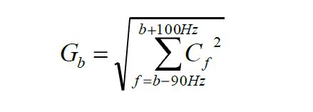
The grouping of the signals is a result from Parseval’s energy theorem. This theorem states that the signal energy expressed in the time domain is equal to the signal energy in the frequency domain:

An example of the grouping of individual frequency components into 200-Hz bands is shown in Figure 8.1.

Figure 8.1 Grouping according to IEC 61000-4-7 in the range from 2 to 9 kHz.

The difference from the traditional harmonic measurements (below 2 kHz) is that the distortion below 2 kHz has in most cases more of a line spectrum character, whereas in the higher frequency range the distortion is more likely to have a continuous spectrum. The methods for grouping of harmonics below 2 kHz compared with the method for grouping in the range from 2 to 9 kHz give the same results for a single frequency distortion (line spectrum). But when the signal is more continuous, the results will differ between the methods.

The standard document recommends the use of a filter when measuring in the frequency range 2 to 9 kHz to remove the low-frequency parts of the distortion. The use of a 24-bit A/D converter can be an alternative to the use of such a filter. The additional 10 bits in resolution provide about 60 dB extra dynamic range compared with a measurement using a 14-bit A/D converter. As the suppression of the fundamental component should be 55 dB according to the standard, the remaining dynamic range for the distortion in the range 2 to 9 kHz is about the same.

8.2 CISPR 16

CISPR contains emission limits, both for radiated and conducted disturbances, and also immunity tests against these disturbances. CISPR 16 mostly takes into consideration disturbances in the frequency domain, and therefore measurement with measuring receivers is most common. The standard deals with measurements from 9 kHz to 18 GHz. The frequency spectrum is divided into different frequency ranges (A to D) where, for example, A is the range between 9 and 150 kHz and B is the range between and 30 MHz.

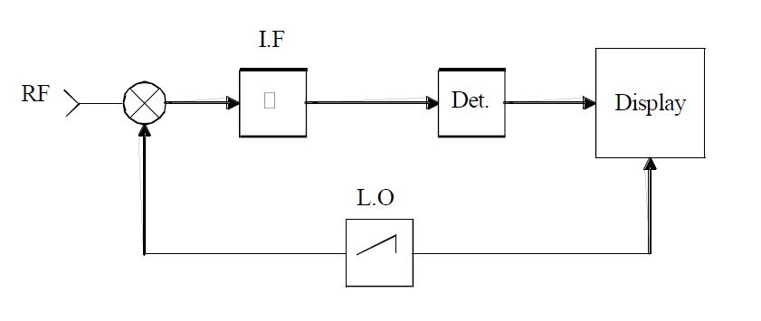
CISPR 16-1-1 (2003) describes the different measuring receivers, and also spectrum analyzers, audio-frequency voltmeters and disturbance analyzers. An explanation of all these apparatuses is not given here, but Figure 8.2 shows a very simplified schematic of a scanning receiver. The “radio frequency signal” is mixed with a signal from a “local oscillator” and then fed through a filter with a predetermined resolution bandwidth (RBW) that filters out the “intermediate frequency”. Then a detector, quasi-peak, peak, average or RMS, decides the amplitude of the signal that is then fed to the display together with the frequency from the “local oscillator”.

Figure 8.2. Simple schematic of a scanning receiver.

The detector can be of different type and some types are:

Quasi-peak is a form of detection in which a signal level is weighted based on the repetition frequency of the spectral components making up the signal. The result of a quasi-peak measurement depends on the repetition rate of the signal. The input is often simplified with a diode in series with a resistor, and then a capacitor in parallel with a resistor; the charging time and discharging time are defined in the standard. Note that there are different time constants for bands A, B and C and D.

Peak is simply a registration of the maximum magnitude recorded during the measurement time. The measurement time (sometimes also called dwell time) determines how long each filter band should be monitored before stepping to the next one. The measurement time is determined from the scan time divided by the total number of frequency bands monitored (CISPR 16-2-1, 2003).

Average is simply designed to indicate the average value of the envelope of the signal passed through the filter.

RMS detects the root-mean-square value of the signal passed through the filter during the measuring time. Note that since the response of an RMS meter is proportional to the square root of the bandwidth for any type of broadband disturbance, the actual bandwidth needs not be specified.

This solution makes it easy to sweep the signal and get the magnitude of each frequency band. But depending of the type of detector and characteristics of the signal, the result will differ. The RBW should be about 200 Hz between 9 and 150 kHz and 9 kHz between 0.15 and 30 MHz, except for measurement with the RMS detectors, as stated above.

8.3 Comparison (DFT vs. measuring receiver)

Measurements in the range up to 9 kHz, according to IEC 61000-4-7 (2002), take a snap-shot of the voltage or current waveform and apply mathematical tools to extract the spectrum. The spectral components are next merged into predefined frequency bands. Measurements above 9 kHz, according to CISPR 16, use a frequency-domain approach in which a receiver sweeps through the whole frequency range, taking one band at a time. The two methods will be referred to here as “IEC method” and “CISPR method”. This difference between the two methods is shown schematically in Figure 8.3.

Figure 8.3. Coverage of time and frequency domain for IEC method (left) and CISPR method (right).

The IEC method takes a time window of the waveform and obtains the values for each frequency band over this window. The CISPR method only takes one band at a time. If the measured signal is stationary (i.e., its properties will not change with time), the two methods will give the same result. But in reality, stationary signals are rare. Many signals are either discontinuous or modulated in some way, and this will lead to different results for the two methods. In defence of the CISPR method it should be mentioned that this method was developed for measuring the emission of equipment. When the equipment is in a fixed operational state, the emission can be expected to be stationary, although this is not guaranteed.

For time-variant signals, the IEC method allows for continuous monitoring, whereas the CISPR method will always have gaps. Again, for emission measurements this may not be a serious concern, but for measurement of the electromagnetic environment (voltage quality), the signals are much more likely to be varying in time.

An important argument for using the CISPR method (and probably the reason it was chosen in the first place) is that it does not put high demands on sampling capacity and on computing power. The CISPR method can cover a very wide bandwidth and has a large dynamic range. It uses basically the same technology as radio receivers, which has been well developed and been widely available for many years. Fast sampling technology and high computing power have only recently become widely available. Actually, digital technology has become so much cheaper that the IEC method may by now be easier and cheaper than the CISPR method for frequencies up to 150 kHz. Note that for the highest frequencies, the CISPR method remains superior.

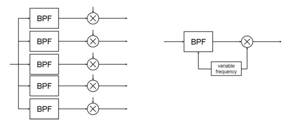
Even for stationary signals, it is not sure that the IEC method and the CISPR method will produce exactly the same results. Actually, STFT and other methods for spectral estimation can be seen as a filter bank as shown on the left-hand side in Figure 8.4. The time signal is fed in to the system in parallel, and each frequency is separated with the filter bank. That means that from each filter we get a time domain signal that we then can give a value in the form of quasi-peak, RMS, peak, average, etc.

Figure 8.4. Schematic principle of IEC method (left) and CISPR method (right).

In both methods, the parameters (i.e., the disturbance level for each band) are obtained from a lowpass filter followed by heterodyning to a baseband (“intermediate frequency” or “IF” in CISPR 16). The disturbance level is next obtained from the level of the baseband signal. If the bandpass filters in the two methods have the same frequency characteristic, the results of the methods will be the same. The bandpass-filter curve is well defined in CISPR for the IF, but it is doubtful that STFT has the same filter curve.

The dwell time specified in CISPR is about 10 ms for a peak detector and 2 s for the quasi-peak detector in the range from 9 to 150 kHz. In comparison with the principle shown schematically in Figure 8.4 for IEC, this means that if we want to have the same dwell time, we would have to use a 10 ms window for peak detection but a 2-second window for quasi-peak.

There are however today measuring equipments in use what we could call a hybrid technology between time- and frequency-domain measurements. The benefit is that it describes both frequency- and time-domain together with the amplitude in a 3-dimentional plot. This gives a better indication on how the frequencies changes with time. There are however also analysing methods (transforms and curve fitting models) which can show how the frequencies changes with time, i.e. STFT, wavelet and some other methods using sliding window. The drawback with these instruments/analyzing-methods is that a high time step leads to a low frequency step and vice versa.

8.4 Proposed measurement technique

We propose to use the time domain for measurements throughout the frequency band 2 to 150 kHz.

9 Conclusions

Based on the measurement of voltage and current distortion, three types of disturbances are recognized in the frequency range 2 to 150 kHz.

Narrowband signals appear mainly in the form of individual frequencies due to power-line communication.
Broadband signals are mainly due to individual end-user equipment with active power-factor correction.
Recurrent oscillations (typically every 10 ms) are due to limitations of the power-electronic converters around the current zero crossing.

We propose to use the time domain for measurements throughout the frequency band 2 to 150 kHz.

10 References

[1] M.H.J. Bollen, P.F. Ribeiro, E.O.A. Larsson, C.M. Lundmark, Limits for voltage distortion in the frequency range 2-9 kHz, IEEE Transactions on Power Delivery, Vol.23, No.3 (July 2008), pp.1481-1487.
[2] R. Gretsch, M. Neubauer, “System Impedances and Background Noise in the Frequency Range 2 kHz to 9 kHz”, ETEP, Vol.8, No.5 (September/October 1998), pp.369-374.
[3] Nätåterverkan av lågenergibelysning, Rapport Energimyndigheten, in print.
[4] Sarah Rönberg, Martin Lundmark, Mats Wahlberg, Markus Andersson, Anders Larsson, Math Bollen, Attenuation and noise level – potential problems with communication via the power grid, Int Conf on Electricity Distribution (CIRED), Vienna, May 2007.
[5] Anders Larsson, High frequency distortion in power grids due to electronic equipment, Licentiate, Luleå, 2006.
[6] E.O.A. Larsson, C.M. Lundmark, M.H.J. Bollen, Distortion of Fluorescent Lamps in the Frequency Range 2-150 kHz, Int Conf on Harmonics and Quality of Power (ICHQP); Cascais, Portugal, October 2006.
[7] A. Larsson, M.H.J. Bollen, M. Lundmark, Measurement and analysis of high-frequency conducted disturbances, Int Conf on Electricity Distribution (CIRED), Vienna, May 2007.
[8] F. Krug, D. Mueller, P. Russer, Signal processing strategies with the TDEMI measurement system, IEEE Transactions on Instrumentation and Measurement, vol. 53, No. 5, October 2004. pp.1402-1408. ISSN: 0018-9456
[9] F. Krug, P. Russer, Quasi-peak detector model for a Time-domain measurement system, IEEE Transaction on Electromagnetic Compatibility, Vol. 47, No. 2, May 2005, pp. 320-326, ISSN: 0018-9375
[10] Application guide to the European Standard EN 50160 on “voltage characteristics of electricity supplied by public distribution systems”, Eurelectric, July 1995.
[11] S. K. Rönnberg, M. Wahlberg, M. H. J. Bollen, C.M. Lundmark, Equipment currents in the frequency range 9-95 kHz, measured in a realistic environment, Int Conf on Harmonics and Quality of Power (ICHQP), Wollongong, Australia, September 2008.