Current and voltage harmonics are often used interchangeably. At most places, only harmonics is quoted and whether the values pertain to current or voltage is not mentioned. The differentiation can be done on the basis of their origin.
Understanding Total Harmonic Distortion
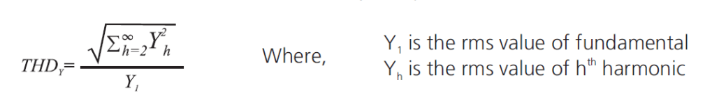
The current and voltage harmonics in a system are often expressed as Total Harmonic Distortion (THD). The total harmonic distortion or THD, of a quantity is a measurement of the harmonic distortion present and is the ratio of all harmonic components to the fundamental component. It is give by the formula as under:
Hence, current THD is the ratio of the root-mean-square value of the harmonic currents to the fundamental current.
Where do Current & Voltage Harmonics Originate?
Harmonics always originate as current harmonics and voltage harmonics are the results of current harmonics. Current harmonics originate because of the presence of non-linear loads like variable speed drives, inverters, UPS, television sets, PCs, semiconductor circuits, welding sets, arc furnaces in the system. They act as harmonic current sources. The resulting current waveform can be quite complex depending on the type of load and its interaction with other components of the system.
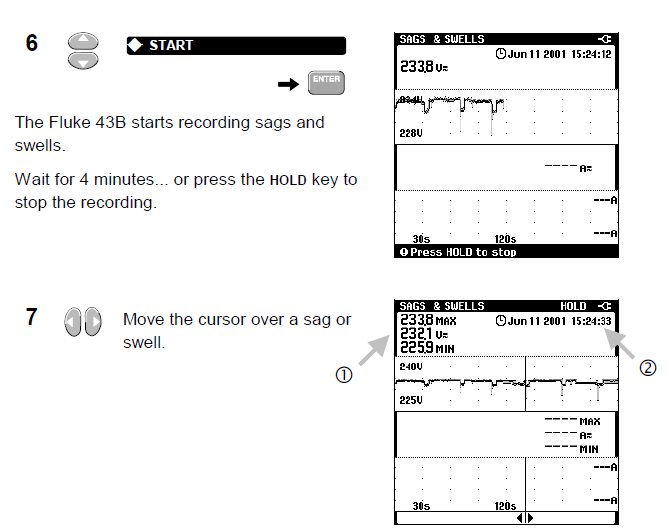
The distorted current waveforms can be represented as the sum of current waveform of fundamental frequency and of its multiple (harmonics):
Voltage harmonics do not originate directly from non-linear loads. The current harmonics (distorted waveform) flow through system impedance (source and line impedances) and cause harmonic voltage drop across the impedances. This will distort the supply voltage waveform. Thus voltage harmonic are generated. Long cable runs, high impedance transformers, etc. contribute to higher source impedance and hence, higher voltage harmonics.
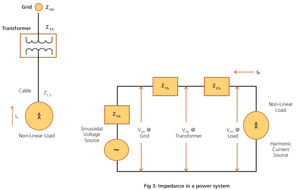
A typical power system has the following impedances as indicated in the line diagram:
In the above diagram,
Vh = hth harmonic voltage
Ih = hth harmonic current
Zh = Impedance at hth harmonic
Vthd = Voltage total harmonic distortion
At load, Vh = Ih x (ZCh + ZTh + ZGh)
At transformer, Vh = Ih x (ZTh + ZGh)
At grid, Vh = Ih x (Zgh)
Usually, grid impedances are very low and hence, the harmonic voltage distortion are also low there. However, they may be unacceptably higher on the load side as they are subjected to full system impedance there. Hence, it becomes important where the harmonics measurements are done.
However, in case of DG sets, the source impedance is large resulting in high voltage harmonics despite small current harmonics. Thus, a clear distinction between current and voltage harmonics becomes important here.
An industry, say industry A, that has large non-linear loads will generate huge current harmonics in its system. A nearby industry, say industry B, connected to the same grid may not have non-linear loads, yet, it may be subjected to high voltage harmonics. These voltage harmonics are the result of high current harmonics of industry A and impedance of grid & transformer. Thus, industry B despite small current harmonics, has high voltage harmonics may also appear in the systems, magnifying voltage harmonics further.
How do Current & Voltage Harmonics Affect the System?
Current harmonics increase the rms current flowing in the circuit and thereby, increase the power losses. Current harmonics affect the entire distribution all the way down to the loads. They may cause increased eddy current and hysteresis losses in motor and transformers resulting in over-heating, overloading in the neutral conductors, nuisance tripping of circuit breakers, over-stressing of power factor correction capacitors, interference with communication etc. They can even lead to over-heating and saturation of reactors.
Voltage harmonics affect the entire system irrespective of the type of load. They affect sensitive equipment throughout the facility like those that work on zero-voltage crossing as they introduce voltage distortions.
Understanding IEEE 519 Guidelines
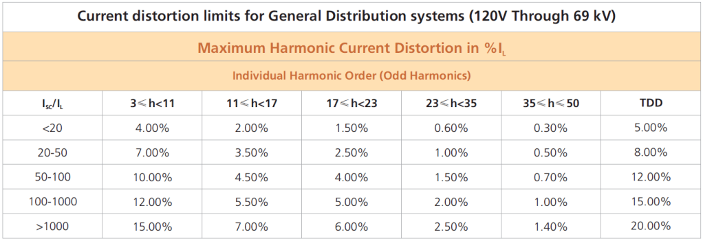
The purpose of harmonic limits in a system is to limit the harmonic injection from individual customers to the grid so that they do not cause unacceptable voltage distortion in the grid. IEEE 519 specifies the harmonic limits on Total Demand Distortion (TDD) and not Total Harmonic Distortion (THD). TDD represents the amount of harmonics with respect to the maximum load current over a considerable period of time (not the maximum demand current), whereas, THD represents the harmonic content with respect to the actual load current at the time of measurement.
It is important to note here that a small load current may have a high THD value but may not be significant threat to the system as the magnitude of harmonics is quite low. This is quite common during light load conditions.
TDD limits are based on the ratio of system’s short circuit current to load current (ISC/IL). This is used to differentiate a system and its impact on voltage distortion of the entire power system. The short circuit capacity is a measure of the impedance of the system. Higher the system impedance, lower will be the short circuit capacity and vice versa.
The Guidelines IEEE 519-2014 at PCC Level are as under:
where
ISC = maximum short-circuit current at PCC [Can be calculated as MVA/(%Z x V)]
IL = maximum demand load current (fundamental frequency component) at PCC
Systems with higher ISC/IL have smaller impedances and thus they contribute less in the overall voltage distortion of the power system to which they are connected. Thus, the TDD limits become less stringent for systems with higher ISC/IL values. In other words, higher the rating of transformer used for the same amount of load, higher will be the allowable current distortion limits.
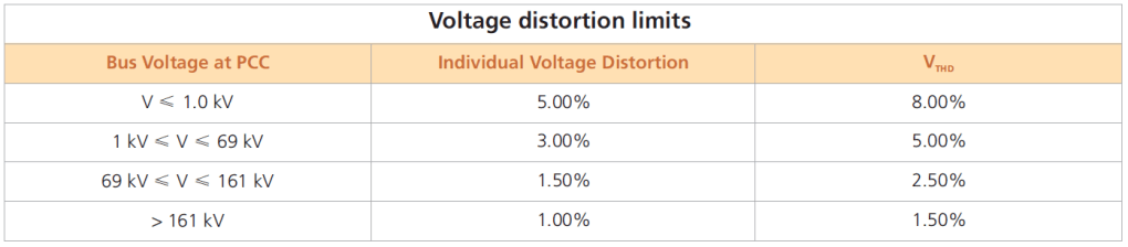
The limits on voltage are set at 5% for total harmonic distortion and 3% of fundamental for any single harmonic at PCC level. Harmonics levels above this may lead to erratic functioning of equipment. In critical applications like hospitals and airports, the limits are more stringent (less than 3% VTHD) as erroneous operation may have severe consequences. As discussed already, the harmonic voltage will be higher downstream in the system.
Solutions for Current & Voltage Harmonics
**These are typical solutions. However the actual solution may vary depending up on the actual harmonic content in the system.
Ir. M. van Lumig, Electrical Power Systems, Analysis and Concepts Laborelec NL Beek-Maastricht Airport, the Netherlands, e-mail: michiel.vanlumig@laborelec.com
Ir. S. Bhattacharyya, Electrical Energy Systems Group Technical University Eindhoven Eindhoven, the Netherlands, e-mail: s.bhattacharyya@tue.nl
Dr. ir. J.F.G. Cobben, Electrical Energy Systems Group Technical University Eindhoven Eindhoven, the Netherlands
Prof.ir. W.L. Kling, Electrical Energy Systems Group Technical University Eindhoven Eindhoven, the Netherlands
This paper describes the results of a four years (2006-2010) Power Quality (PQ) monitoring campaign conducted in the Dutch networks. Purpose is to get insight in the PQ at the point of connection (POC) of some connected customers with typical characteristics as for example distributed energy resources (DER) and to compare these results with the limits given in the EN50160. The results show however no specific problems near a large amount of photo voltaic (PV) panels. There was no correlation found between the harmonic distortion of the grid voltage and the production of solar energy. Pst levels are slightly higher on semi-cloudy days, but due to the low grid impedance never exceed the standard limits. Also near wind turbines no problems with the PQ are visible. The PQ near disturbing loads, like variable speed drives (VSDs), shows higher 5th and 7th order harmonics on MV level. Overall, because of the usually strong Dutch grids, no PQ problems were measured at the specific locations.
Keywords: Power Quality (PQ); distributed energy resources generation (DER); point of connection (POC); EN50160; PQ monitoring.
1. Introduction
The paper describes the results of the PQ monitoring campaign within the EOS-LT ‘Voltage Quality of the Future Infrastructure’ (KTI) project [1]. A four-year measurement campaign is being carried out, acquiring Power Quality (PQ) data at 20 different locations in the Dutch LV, MV and HV grids. Purpose is to get insight in the PQ at the Point Of Connection (POC) of some connected customers with typical characteristics as for example distributed energy resources (DER) and to compare these results with the limits given in the EN50160 [2] and Dutch ‘Grid Code’ [3]. The requirements in the Dutch Grid Code, at some points, are different from the requirements in the EN50160. The most important differences are the requirements on flicker (Plt <5 for 100% of the time), THD(U) and 5th order harmonic voltages. All differences between the EN50160 standard and the Dutch ‘Grid Code’ are given in Table 1.
Table 1 Main differences between the EN50160 standard [2] and the Dutch ‘Grid Code’ [3]
Parameter
Dutch Grid Code
EN50160
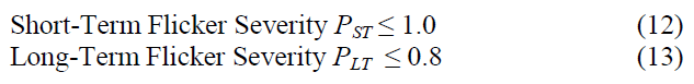
Flicker severity
Plt≤ 5 for 100% of the time
Plt≤ 1 for 95% of the time
Voltage unbalance
Negative sequence voltage <3% of the positive sequence during 100% of the time
Negative sequence voltage <2% of the positive sequence during 95% of the time
Total harmonic voltage distortion
THD(U) ≤ 12% during 99.9% of the time
THD(U) ≤ 8% during 95% of the time
5th harmonic voltage
9% for the 99.9% of the measurement period
6% for 95% of the measurement period
Fast voltage variations
≤10% Un; it is ≤3% Un in situations without loss of production
As per IEC 61000-3-3 limits relative steady state voltage change ≤3.3% Un
2. Details Measurement Equipment
The equipment used in the monitoring program measures according to the EN 61000-4-30. A UPS (12V/1,2 Ah) is integrated to have an average autonomy of 30 minutes. All devices are equipped with a GSM/GPRS modem for communication with the central database. Downloading of the measurement data is performed every day, while the internal memory is 512 MB (enough for 2 month measuring when recording 10 minutes RMS data). The data is analyzed following the standard EN 50160 and the influence of the connected load on the voltage is analyzed.
3. Measurement locations
The measurements locations were chosen in the neighborhood of DER, household loads or disturbing loads such as a stone factory (flicker) and a plastics factory (harmonics). In this way, the measurements give insight in possible future PQ levels in the neighborhoods with DER or new (disturbing loads). Measurements are carried out at the POC of different customers and/or DER. The locations changed during the measurement period according to the needs within the project. The most important PQ monitoring locations are shown in Table 1. The PQ performance of all of the measurement locations will not be discussed in detail. The main focus in this paper is on photo voltaic (PV) installations, wind turbines, other ‘possible problem’ locations and household areas.
Table 2 PQ monitoring for ‘KTI’ project
Measurement Location
Main PQ parameters
1 Wind turbine (LV)
Voltage variation, flicker
1 Wind turbine feeder (MV)
Voltage variation, flicker
1 Wind turbine feeder (MV)
Harmonics, voltage variation
7 locations with households/small commercial customers (LV)
Harmonics, flicker
1 Stone factory (LV)
Flicker
1 Plastic factory (LV)
Harmonics
3 Green houses with CHP/lighting (LV+MV)
Harmonics, voltage variation
1 Connection to railway (HV
Unbalance, asymmetry
1 Bio-energy plant (MV)
Harmonics
1 Micro CHP (LV)
Harmonics, flicker
4. Measurement Results
In this chapter the main results of the PQ measurement campaign will be discussed. Focus is on finding the relation between the PQ phenomena and the disturbing sources, like PV inverters and power electronics.
A. PQ near PV panels
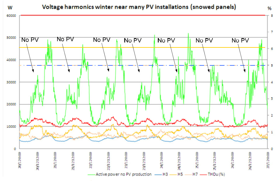
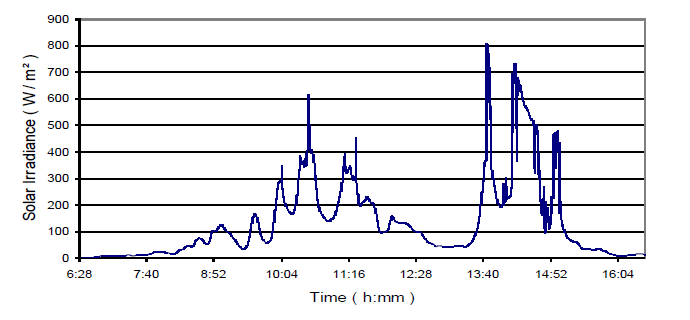
Three of the measurement locations are near large amounts of PV inverters. The inverters are single phase. Depending on their design and grid impedance, the inverters cause distortion on the grid voltage. To correctly analyze the caused distortion, two situations are compared: 1) summer situation with high PV production (Fig. 1) and 2) winter situation with no PV production due to snow on the panels (Fig. 2). In this way harmonics caused by other household equipment are comparable.
Fig. 1 THDu (%) (red), 3rd, 5th and 7th harmonic (blue, orange, rose) and feeder loading (green) in summer
Fig.1 and Fig. 2 clearly show that the harmonic distortion on the voltage is low in the neighborhood of many PV panels. In summer, during sunny days, the THDu (%), the Total Harmonic Distortion of the RMS voltage, is about 2.5%, in winter time about 1,7%. This extra distortion seems to be caused by the PV inverters, but the influence is very small. A third order harmonic voltage, caused by many rectifiers used in household equipment, is clearly visible and increases during peak demand. The main harmonic voltage is the fifth, but still well below the limits of the Dutch ‘Grid Code’.
Another interesting parameter is the voltage level at the end of a feeder near many PV panels. The phase-to-neutral voltage never reached a level above 240V at the measurement location, but the correlation between grid voltage and PV production is clearly visible. In grids with higher impedance or even more installed PV panels, grid voltage could reach critical levels. This has not been measured at the measurement locations.
Fig. 2 THDu (%), 3th harmonic and feeder loading in winter
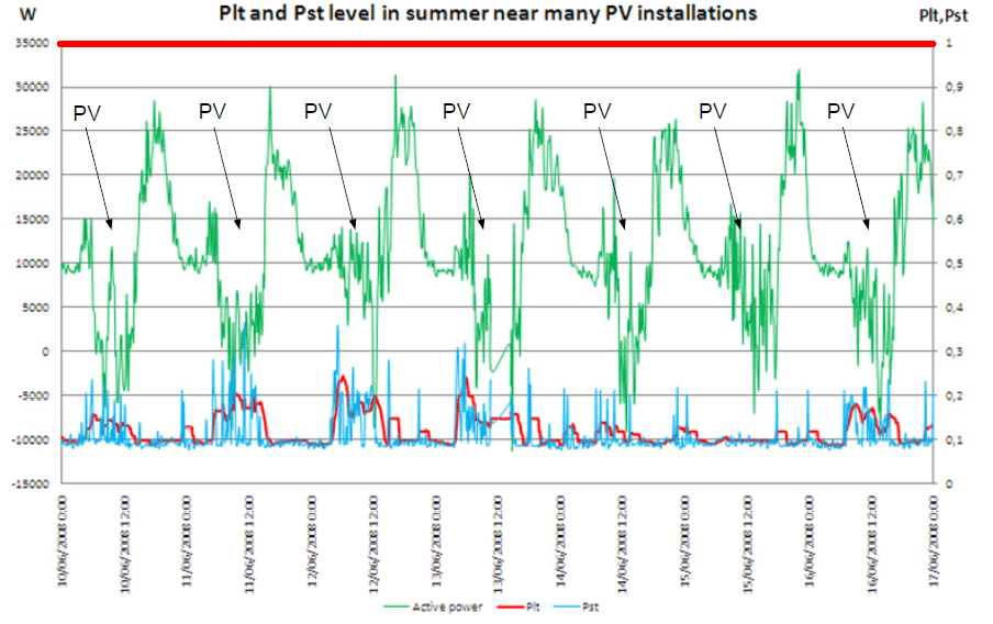
On semi-cloudy days PV panels are subject to variations in sun irradiation and therefore the PV production will vary accordingly. The measurements show indeed a higher Pst and Plt level, but well below the limits of the Dutch ‘Grid Code’ (Fig. 3).
Fig. 3 Pst , Plt and loading of the feeder in summer
B. PQ near wind turbines
Wind turbines are connected to the grid via power electronics which, when not properly designed, can cause harmonic distortion on the grid voltage. To analyze this effect two measurements are carried out, one at the terminals of a 600 kW wind turbine and one at the end of a MV feeder with many wind turbines connected.
Fig. 4 Harmonic currents produced by a 600 kW wind turbine at nominal power
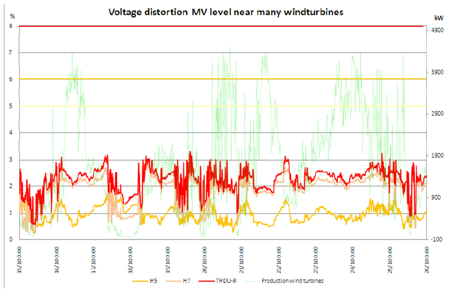
In Fig. 4 the 5th, 7th, 13th and 15th harmonic currents are clearly visible. This spectrum of harmonic currents is typical for a 6-pulsed bridge. The distortion of the grid voltage is low, the measured THDu (%) is between 1% and 3%. Because there are many wind turbines connected to this feeder, the influence of one wind turbine could not be distinguished. Also at the beginning of the feeder the measured voltages and currents were analyzed (Fig. 5).
Fig. 5 THDu (%) measured at MV level near many wind turbines
From this figure it’s hard to find any correlation between wind production and the THDu (%) level. Therefore is looked at different situations with increased production of wind power. The average value of THDu (%) is calculated in these intervals for 2010.
Fig. 6 THDu (%) on MV level in function of wind power production
Fig. 6 shows an increase in THDu (%) with increasing wind power, but after an increase to about 2% it stays somewhat constant with increasing power production.
Another PQ parameter which might be increased by wind turbines is the flicker level Plt. High current peaks due to wind surges can cause Plt levels to increase. This is analyzed in Fig. 7. There is some correlation found between the max or ΔI current drawn and the flicker levels. But on average there was very little Pst caused by the wind turbines. At some specific events the Pst increased suddenly, these were analyzed to find out whether the Pst level came from other feeders or HV. At these specific moments the Pst was high, caused by sudden voltage distortion. This voltage distortion was caused by 3rd order harmonic voltages. At the same time there was no 3rd order harmonic current increase from the wind turbines. The cause of the sudden voltage distortion on MV level is still unknown.
Fig. 7 Pst and Plt level at MV near many wind turbines
C. PQ level near a stone factory
The PQ level is not only influenced by DER, loads play an important part in disturbing the grid voltage. Nonlinear loads, which draw a non-sinusoidal current, can cause voltage distortion in the form of harmonic voltages. Loads also can cause sudden voltage dips, due to high currents compared to the short-circuit power available. One of the measurements is carried out at the LV-side of a transformer connecting a stone factory. Because of the processes in this factory, high currents are regularly drawn from the grid, causing a high Plt level (Fig. 8).
Fig. 8 Pst and Plt level at the POC of a stone factory
In Fig. 8 it can be clearly seen that there is a one to one correlation between the power drawn and the Pst and Plt levels. Also it’s clear that the company is not producing in weekends, and the power and flicker level is at much lower levels. Although the Plt level was not above limits, the grid operator changed the grid topology at this location to solve the problem.
D. PQ near a plastics factory
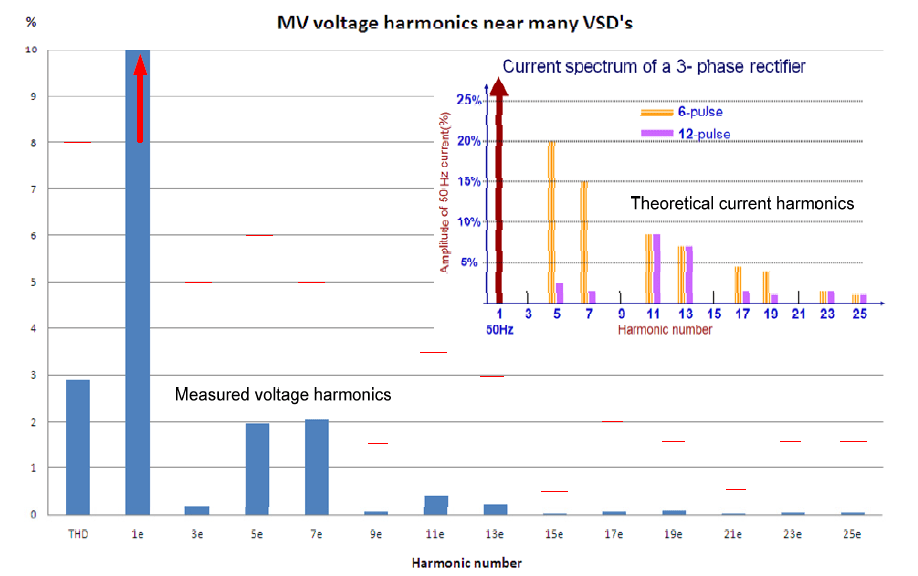
High currents can cause dips, rapid voltage fluctuations can cause flicker. But another increasing problem is the non-linear currents drawn by power electronics used in many loads. In fact any equipment using DC voltages and connected to the public grid has non-linear elements. Examples are power sources used in PCs, flat screen panels and energy saving lamps. These sources are mainly one phase and draw currents with large peaks to maintain the DC-bus voltage. In industry also more and more nonlinear loads are connected, like variable frequency drives. These drives, in most cases 6-pulsed, can cause high harmonic currents when not a correct filter is used. A typical layout of a 6-pulsed bridge is shown in Fig. 9.
Fig. 9 Typical layout of a 6-pulse bridge
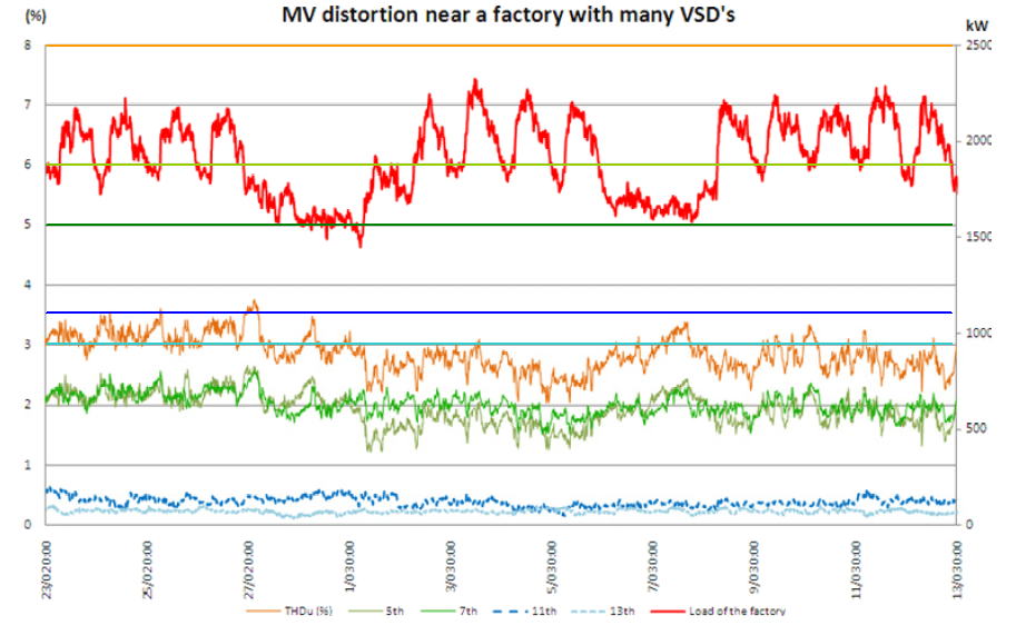
To measure the influence of many variable speed drives (VSDs) on the grid voltage, a measurement is carried out at MV level near a plastics factory with many VSDs. This measurement is shown in Fig. 10.
Fig. 10 Harmonics at MV level near many VSDs
The THDu (%) at MV level varies between 2% and 4% and is mainly caused by 5th, 7th, 11th and 13th order harmonic voltages. This can be seen in Fig. 11. The harmonic voltages are caused by the harmonic currents drawn by all VSDs together. The harmonic current spectrum of a 6- and 12-pulsed drive is shown in the picture in Fig. 11.
Fig. 11 Harmonic voltage spectrum at MV level near a plastics factory
Although the THDu (%) is below 8%, it’s important to notice the effect of the VSDs on MV level. Reducing the harmonic currents with effective filtering would help to reduce the harmonic voltage distortion. This is important because a distorted grid voltage can cause damage and extra losses in equipment.
E. PQ in a household area
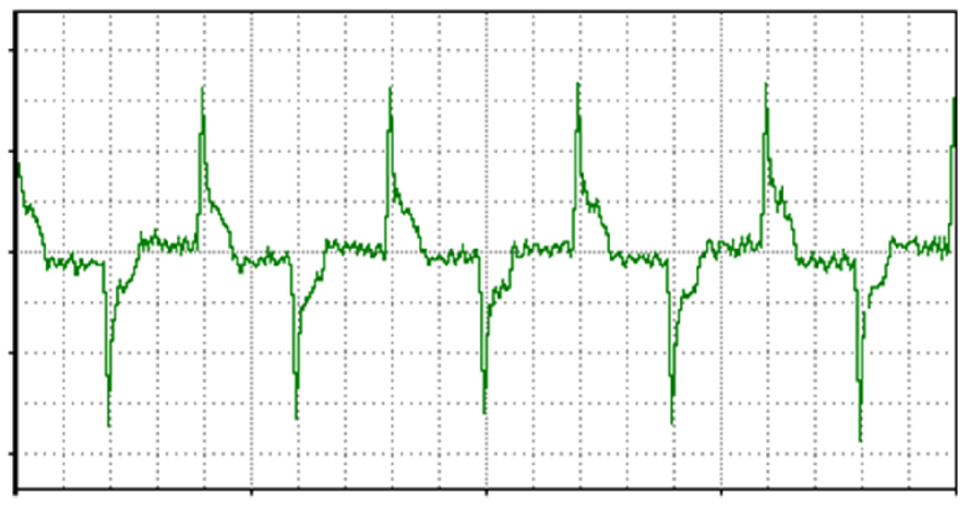
Almost all household equipment nowadays uses power electronics and this will increase in the future. Not only there will be more electronic devices, also resistive devices like the well known incandescent lamp is more and more replaced by energy saving lamps, which uses a driver with non-linear elements. The main source of harmonic currents in a household is coming from electronic power supplies. These power supplies, depending on type and brand, inject harmonic currents in the grid. In most cases, these currents have influence on the grid voltage. Most of the household appliances are of single-phase rectifier configuration and have a typical current characteristic as shown in Fig. 12.
Fig. 12 Current drawn by a typical power source
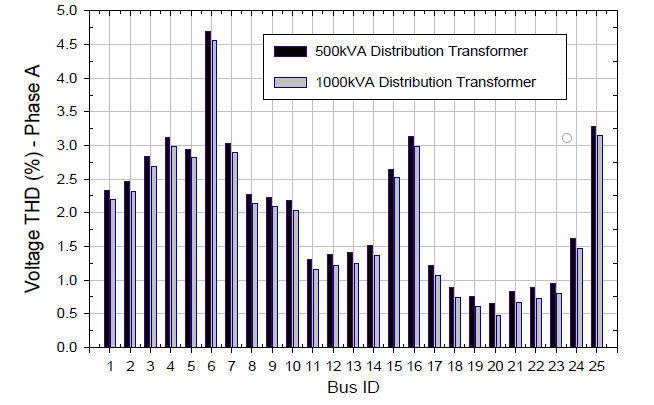
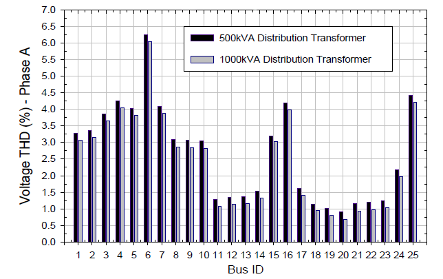
As the power demand of an electronic power source is low, a single device does not cause problem in the grid voltage. It will also individually meet the limits of standards. However, many of such devices in a neighborhood can have significant influence on the grid voltage. Therefore a measurement at the LV level of a 400 kVA transformer is performed in a neighborhood with households and some small shops. The results are shown in Fig. 13.
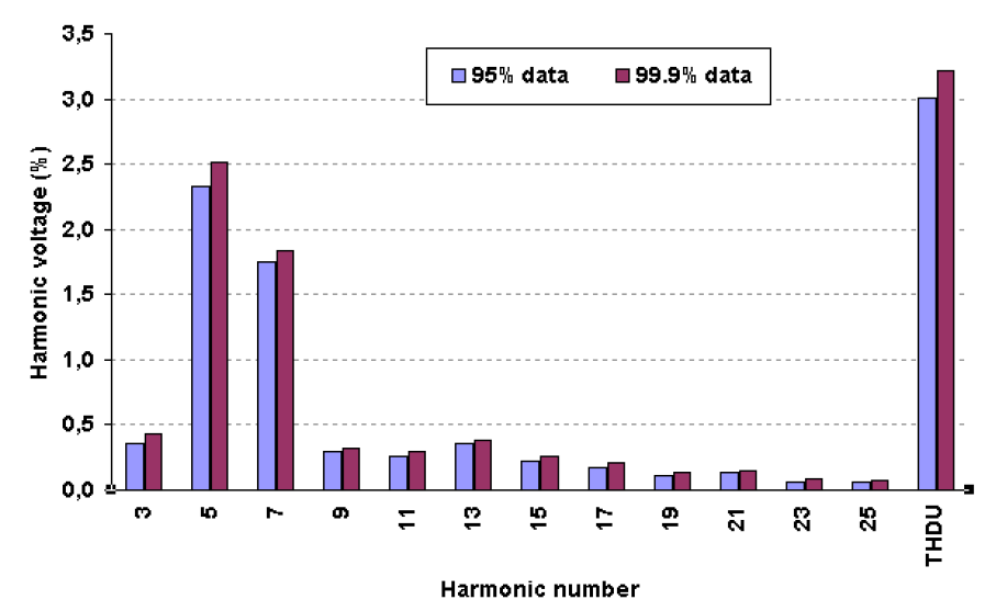
Fig. 13 Harmonic voltage spectrum at the LV side of a 400 kVA distribution transformer
The THDu (%), the most left column, is on average 2.1% and never exceeds 3%. The main harmonic voltages are 3rd, 5th and 7th. All are well below the limits. In Fig. 14 the 95% and 99.9% probability values are given for a household located at the end of a LV cable.
Fig. 14 95% and 99.9% probability values at a household POC located at the end of a LV cable
Other measurements in household areas confirm these levels. There are of course examples of higher values, but the measurements at the specific locations show no alarming results.
Therefore, at present, all voltage harmonic values meet the EN50160 and Dutch ‘Grid Code’ limits. However, one remark can be made about the voltage limits given for higher order harmonics. As per the standards, the 15th and 21st harmonics voltage limits are quite low (only 0.5%) in comparison to the limits given for (13th, 17th, 19th, and 23rd harmonics). The limiting value of 13th harmonic is 3%, whereas that for 17th is 2%. The limits for 19th, 23rd and 25th are 1.5%. From the measurements, these values are all comparable as shown in Fig. 14. Similar observation is made at many measuring locations in the LV network in the Netherlands and also in other networks of the world [4], [5]. Therefore, in future, the limits for 15th and 21st harmonics would probably be needed to modify.
The flicker levels Plt and Pst are also well below the limits of the Dutch ‘Grid Code’, see Fig. 15 and 16.
Fig. 15 Pst and Plt level at the LV side of a 400 kVA distribution transformer
Fig. 16 Frequency of flicker severity levels at a household POC located at the end of a LV cable (one week’s data)
From Fig 16, it can be seen that the probability distribution of Pst and Plt values remain within the range of 0.2-0.3 during the measurement period (of one week). It is similar to the observation that is recorded at the LV side of the distribution transformer (refer Fig. 15).
In the national monitoring program of the Netherlands, voltage dips are mainly recorded in the HV networks. A continuous PQ measurement is needed for a duration of minimum 2-4 years to register voltage dip characteristics at a site. Under the ‘KTI’ monitoring campaign, MV sites are also measured. The equipment used for measuring PQ levels is programmed to detect events, like dips, surges, and crossing programmed limits for other PQ parameters. During the measurement campaign many events were recorded, mainly without knowing the reason for the event.
But one measurement in a specific rural area, known for PQ problems, showed indeed a lot of disturbances. A voltage dip-duration table of one year measurement is shown in Fig. 17.
Fig. 17 Voltage dip duration (DisDip) table from an area with a ‘weak’ grid (1 year period)
In total 135 events were registered in one year, of which 104 were of the category dips.
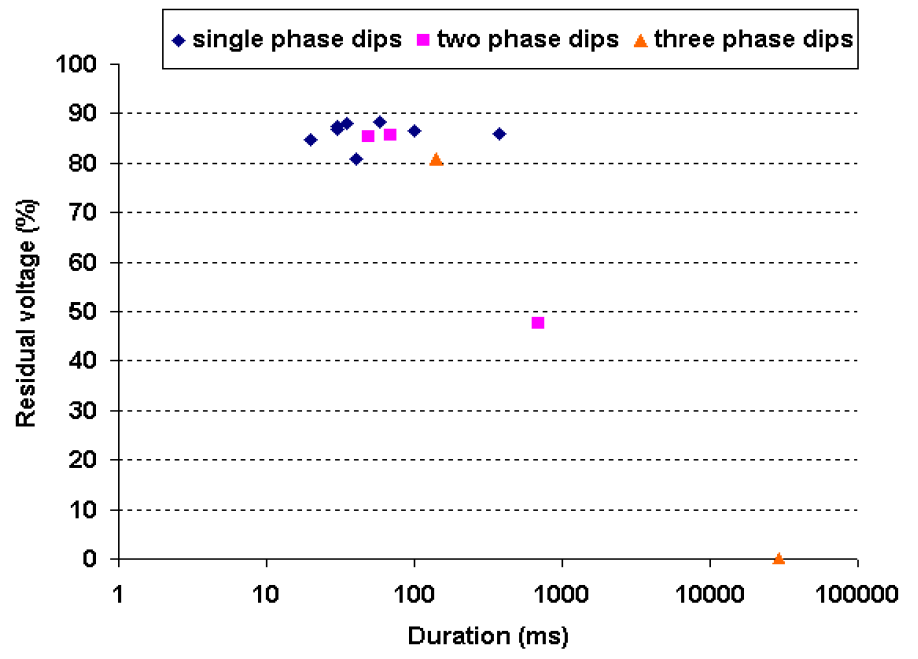
The measurement conducted at an industrial site (stone factory) also recorded voltage dip events during a two years period. Fig 18 shows various single-phase, two-phase and three phase voltage dips events that were measured at the above site. It can be noticed that most of the dips have a residual voltage of 80% or more. Therefore, the specified customer did not suffer any significant financial loss at his installation. It can be remarked here that for a sensitive customer (such as a semiconductor plant), even such type of voltage dips can also cause process failure. Therefore, suitable mitigation methods should be applied there to prevent the installation’s equipment mal-operation and process interruption.
Fig. 18 Voltage dips recorded at the stone factory (2 years period)
5. Conclusion
The main results of the PQ measurement campaign within the EOS-LT KTI project are discussed in this paper. First of all, all measurements did comply with the EN50160 standard and the Dutch ‘Grid Code’ requirements, and the PQ level at the chosen locations was satisfactory. It is satisfactory although the locations were chosen to measure suspected PQ problems at ‘problem’ areas. The main reason for not finding any problems is the grid situation at the specific measurement locations. At the locations with many DER units, the grid was designed accordingly and in general Dutch grids can be regarded as strong.
But, there are clearly correlations found between connected sources/loads and the PQ level. In the case of a large amount of PV panels, the THDu (%) was higher during PV production. Also Plt levels clearly increased during semi-cloudy days. The maximum voltage level was never reached, but there are cases known in which problems occurred.
Also at the measurement location with wind turbines, some PQ parameters were influenced, such as a slightly higher Plt level and rise in harmonic distortion. But, it must be said again, the PQ of the grid at the measurement locations was good.
To be ‘sure’ to find PQ problems, two measurements were carried out at known ‘problem’ areas. The measurement indeed showed high levels of Plt and THDu (%) respectively, which could lead to problems at customer’s sites.
The measurements in household areas, connecting increasingly non-linear loads, showed that households cause little distortion on the grid voltage and the Plt levels are also well below the limits. But with the increase of connected power electronics, harmonic voltages will rise when not correctly filtered. Therefore it’s important to monitor such parameters and investigate in mitigation devices and/or to reduce the production of harmonic currents. In the measurement campaign also events were registered. They play an important role for certain sensitive customers. At a location with a weak grid many events were recorded. At such location a sensitive customer, like a semiconductor plant, can’t be connected without changing grid topology or suitable mitigation devices.
From the four-year measurement campaign can be concluded that the PQ level at the measurement locations is meeting the limits of the Dutch ‘Grid Code’. Because the Dutch grid is usually ‘strong’, no PQ problems were recorded at the chosen locations with many PV panels or wind turbines. But, at other locations problems could occur when no attention is paid to the quality of the connected customers and the grid impedance at that point.
Acknowledgement
The work presented in this paper is part of the research project ‘Voltage quality in future infrastructures’- (‘Kwaliteit van de spanning in Toekomstige Infrastructuren (KTI)’ in Dutch), sponsored by the Ministry of Economic Affairs of the Netherlands.
References
[1] EOS Research program at the TU/Eindhoven: “Voltage Quality of the Future Infrastructure” (KTI). website:\ (www.futurepowersystems.nl) [2] European standard EN-50160, 1994, “Voltage characteristics of electricity supplied by public distribution systems”, CENELEC, Belgium. [3] DTE Grid Code legislation, DTE (Dutch office for Energy Regulation), 2005, http://www.nma-dte.nl:DTE (available in Dutch language only) [4] Council of European Energy Regulators (CEER), “4th Benchmarking report on quality of electricity supply 2008”, ref: C08-EQS-24-04, Brussels, December 2008. [5] P. Issouribehere, A. Galinski, D. Bibé, and G. Barbera, “Ten years of harmonic and flicker control by IEC normalized measurements in Buenos Aires distribution system”. Proceedings of 19th International Conference and Exhibition on Electricity Distribution (CIRED 2007), Vienna, May 2007.
Sonali N. Kulkarni is a Research Scholar, Electronics & Telecommunication Engineering, Rajiv Gandhi Institute of Technology, Versova, Andheri (W), Mumbai, Maharashtra, India.
Prashant Shingare is working as Director of Wind Energy, Emerson Network Power India Pvt Ltd, NITCO Business park, Wagle Industrial Estate, Thane (W), Maharashtra, India.
Over the past three decades global energy consumption has increased drastically due to industrialization, automation of various systems and rise in utilization of domestic machine appliances. In order to fulfill the increasing power demand, the power sector is looking for renewable energy sources as an alternative to conventional sources. The Renewable Energy is generated using distributed generation. Renewable Energy is unpredictable, non storable and intermittent due to varying nature of natural resources. Today’s biggest challenge is to accommodate excess generation of Renewable Energy into existing power system without disturbing power quality. The power quality and hence stability of power system gets affected due penetration of Renewable Energy and loading effect of transmission lines corresponding to small disturbances. Therefore, it is a challenging task to maintain healthy, reliable and smart electrical power transmission and distribution system. This paper deals with the power quality parameters, challenges in Renewable Energy grid integration and the possible solutions to maintain power quality.
Keywords: Distributed Generation, Frequency variation, Grid Integration, Grid Stability, Harmonic Distortion, Low Voltage Ride Through, Micro Grid, Power Quality, Renewable Energy, Smart Grid, Voltage Sag.
1. Introduction
Over the past three decades, global energy generation and consumption have accelerated to unprecedented degrees. In India a large amount of electricity is used for residential, commercial and industrial processes applications every day. Today’s increasing power demand, power crises due to scarcity of conventional sources and impact of conventional source on environment are some of the reasons for paying more attention towards renewable energy sources. The renewable energy sources like wind and solar offers alternative sources of energy, which are in general pollution free, technologically effective, environmentally sustainable and provides electricity without giving rise to carbon dioxide emissions (Shafiullah, et al, 2013). However, most of the existing grid networks consisting of transmission and distribution networks are not capable to handle excess penetration of renewable energy. In power system most of the complexities occur due to the interconnections of different types of power generators, transmission lines, transformers, and varying nature of different loads (Sandhu and Thakur, 2014). The stability and power quality of power system gets affected due interconnection of unpredictable nature of different generators, fluctuating load, loading effect of transmission lines etc. Therefore, it is very challenging to maintain reliable and healthy power system irrespective of different uncertainties.
The rest of the paper is organized as follows: Section 2 reviews background and customers of power quality. In Section 3 different power quality parameters are discussed. The cost of poor power quality is reviewed in section 4. The possible solutions to power quality problems are discussed in Section 5 followed by the conclusion.
2. Background
In order to fulfill the increasing demand of electricity, power sector is using several renewable energy sources like wind energy, photovoltaic energy, wave energy, tidal energy etc. along with the conventional sources for power generation. Renewable energy generation is unpredictable and intermittent in nature; it is therefore a challenging task to integrate renewable energy resources into the power grid without affecting power quality. In power system most of the complexities occur due to the interconnections of various types of power generators, transmission lines, transformers, and load (Sandhu and Thakur, 2014). The stability of power grid gets affected due to integration of renewable energy, generated in distributed manner.
Distributed Generation (DG) is used to minimize the losses and loading effect of transmission lines. The distributed generation is the recent trend of distribution network service providers, in which significant power generation is done near the distribution level. Integration of distributed generation causes bidirectional power flow among the network, which reduces the capacity of feeder and transmission line (Enslin, 2010). The other benefits of distributed generation include the reduction of power loss, better voltage support, peak shaving and the improvement of overall efficiency, stability and reliability of the power system (Enslin, 2010), (Roy, et al, 2011).
The renewable energy generation is unpredictable and intermittent in nature hence; it is a challenging task to integrate renewable energy resources into the power grid without affecting power quality. The challenges and issues associated with the grid integration of various renewable energy sources particularly wind energy conversion systems are described in terms of power quality (PQ) (Ackerman, 2005).
2.1 Power Quality Customers
Power quality sensitive customers are grouped into three categories as (Darrow and Headman, 2005):
1.Digital customers: The organizations like banks, stock market, airline reservation systems and corporate offices that rely heavily on data storage and retrieval, data processing, or research and development, need to protect computers, peripherals, and computer cooling equipment. The companies involved in communications facilities like television and radio stations, internet service providers, cellular phone stations, and satellite communication systems need electricity for their computers, peripherals and broadcasting equipment’s to ensure smooth operation of the systems.
2.Continuous Process Industries: The continuous product manufacturing industries like chemical, petroleum, rubber, plastic etc., require continuous supply of electricity during manufacturing to ensure product quality and protect their equipment’s and computers.
3.Other Essential Services: This includes other manufacturing industries, transportation facilities, water and waste water treatment, and gas pipelines.
2.2 Power Quality
Power quality is the term used to describe how closely the electrical power delivered to customers corresponding to the appropriate standards which operates end user’s equipment correctly. Power Quality is a measure of ideal power supply. Power Quality is defined as any power problem manifested in voltage, current, and/or frequency deviations that results in the failure and/or mal-operation of end users equipment (Velayutham, 2015). Due to poor power quality individual consumer suffers, industry suffers which affects the economy of nation (Velayutham, 2015). The penetration of renewable energy into existing power grid is increasing exponentially. Due to the high penetration level of renewable energy like wind, solar etc, in distribution network, the power sector is concerned about the stability of utility grid, power quality (PQ) and voltage regulation (Sandhu and Thakur, 2014). The issues of power quality are of importance to wind energy as an individual unit is of large capacity up to few Megawatts. Further, such a large capacity wind power generator is feeding into distribution circuits, with customers connected in close proximity. The fluctuations in wind speed have a negative impact on power generation, hence on stability and power quality of power system (Singh, et al, 2011). The causes of poor power quality (Velayutham, 2015), (Shingare, 2014) are:
a. Intermittent or unpredictable nature of Renewable Energy generators: The normal operation of wind generator gets affected due to variation in availability renewable sources, adjustable speed drives etc.
b. Variable or Nonlinear loads: The power quality affects due to abrupt changes in load such as start / stop of large motor loads, arc furnaces, lightning, switching devices, traction drives etc.
c. Grid Faults: These are the problems related to grid infrastructure due to ageing of grid network, problems with transmission lines, insulators etc.
3. Power Quality Parameters
The quality of power in distribution grid gets affected due to different types of disturbances at generator side and load side which lead to variation in performance parameters of electrical supply. The parameters of power supply like voltage, frequency are to be monitored continuously. The variation in voltage, frequency and noise level leads to poor power quality. The various parameters of power quality are (Velayutham, 2015), (Almeida, et al, 2013):
1. Voltage sags and swells: Voltage sag is a short duration phenomena in power system in which RMS voltage magnitude decreases between 10 and 90 percent of the nominal RMS voltage at the power frequency, for durations of 0.5 cycle to 1 minute as shown in Fig.1-A.
Fig. 1. A: Voltage sag, B: Voltage swell (Almeida, et al, 2013)
The voltage sag occurs due to faults on the transmission or distribution network (most of the times on parallel feeders). It also occurs due to faults in consumer’s installation, connection of heavy loads and startup of large motors (Tejavoth, et al, 2013).
The voltage swell is momentary or sudden increase of the RMS voltage, at power frequency outside the normal tolerances, with duration of more than one cycle and typically less than a few seconds refer Fig.1-B. It occurs due to start/stop of heavy loads, badly dimensioned power sources, badly regulated transformers (mainly during off-peak hours) (Almeida, et al, 2013).
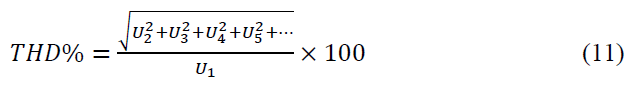
2. Harmonic Distortion: Voltage and current harmonics and sub-harmonics: It corresponds to the supply voltage or current waveforms of non-sinusoidal shape. The waveform corresponds to the sum of different sine waves with different magnitude and phase, having frequencies that are multiples of power system frequency as shown in Fig.2-A. Harmonic distortion causes due different types of nonlinear loads like arc furnaces, welding machines, rectifiers, switched mode power supplies, data processing equipment etc. A common term that is used in relation to harmonics is called as THD or Total Harmonic Distortion (Velayutham, 2015). The term THD is used to describe voltage or current distortion and is calculated using Eq (1) (Velayutham, 2015), (Almeida, et al, 2013):
Where I(Dn) is the magnitude of the nth harmonic as a percentage of the fundamental (individual distortion). The THD is zero for a perfectly sinusoidal wave. It increases indefinitely as the wave form distortion increases. A THD of 5 percent is commonly cited as the border line between high and low distortion for distribution circuits (Velayutham, 2015).
Fig. 2 A: Harmonic Distortion, B: Voltage spike (Almeida, et al, 2013)
3. Voltage Spike: Voltage spike is nothing but a very fast increase in voltage (maximum voltage in the range of thousands) within duration of several microseconds to few milliseconds as shown in Fig. 2-B. The voltage spike causes due to lightening, switching of capacitors, and disconnection of heavy loads. Sometimes, it may damage the electronic components, insulation materials and may cause electromagnetic interference.
4. Voltage Interruptions: A voltage interruption (IEEE Std. 1159), supply interruption (EN 50160), or just interruption (IEEE Std.1250) is a condition in which the voltage at the supply terminals is close to zero. As defined in IEEE, Close to zero means lower than 10 percent of its nominal supply (IEEE Std.1159) (Tejavoth, et al, 2013). The Voltage interruptions can be for short duration or long duration. They are normally initiated due to tripping or failure of protection devices. If the voltage supply interruption occurs from few milliseconds to one or two seconds, it is called short duration interruption as shown in Fig. 3-A (Almeida, et al, 2013). If the supply voltage interruption persists for greater then one or two seconds, it is called long duration interruption shown in Fig.3-B (Almeida, et al, 2013).
Fig. 3 A: Voltage Interruption (Short duration), B: Volt-age Interruption (Long duration) (Almeida, et al, 2013)
5. Voltage unbalance: A voltage unbalance in a three phase system means the magnitudes of three voltages are different and the phase difference between them is not equal to 120 degree refer Fig.4-A. It causes due to unbalanced load in three phase system. The most affected loads are three phase induction machines (Almeida, et al, 2013).
Fig. 4 A:Voltage Unbalance, B: Noise (Almeida, et al, 2013)
6.Noise: Noise is superimposing of high frequency signal on the power supply waveform as shown in Fig.4-B. There are various causes or sources of noise in the power system like electromagnetic interference, radiations due to welding machines and furnaces etc. Usually noise is not destructive but it may cause data processing errors and disturbance to sensitive equipments (Almeida, et al, 2013).
7.Flickers and fluctuations: During normal operation, wind turbines produce a continuously variable output power as result of fluctuation in wind speed (Ackerman, 2005). The random nature of wind resources, in the wind farm generates fluctuating electric power. The fluctuating electric power when injected to the power grid leads to the variation of wind farm terminal voltage due to system impedance.
This power disturbance propagates into the power systems and can produce a phenomenon known as flicker, which consists of fluctuations in the illumination level caused by voltage variations. The oscillation of RMS voltage value, amplitude modulated by a signal with frequency of 0 to 30 Hz (Almeida, et al, 2013).
8.Frequency deviations: Frequency deviation is the variation of relatively small frequency value around its nominal or ideal value. Supply frequency is one of the most critical parameter of the power system. Controlling supply frequency is one of the most challenging part of power system (Velayutham, 2015). There are various reasons for supply frequency deviation.
9.Power factor: The concept of power factor originated from the need to quantify how efficiently a load utilizes the current that it draws from an AC power system. The true power factor at the load is defined as the ratio of average power to apparent power. In AC (sinusoidal) supply with linear load, it is called displacement power factor. With a non sinusoidal supply, the true power factor is influenced by current harmonics and a distortion power factor is included apart from displacement power factor. In order to improve power factor in a harmonic environment filter associated capacitors are used (Velayutham, 2015). The basic technical challenge comes from the variability of wind and solar power which affects the load, generation balance, varying demand for reactive power and voltage stability.
4. Cost of Poor Power Quality
The costs of power quality problems are highly dependent of several factors, like the business area, sensitivity of the equipment used in the facilities and market conditions etc. A huge financial loss occurs due to power quality problems. Generally all the electricity consumer loads are not sensitive to power quality variations (Darrow and Headman, 2005). Therefore, the type of load will depend on size of the sensitive load with respect to the entire load (Darrow and Headman, 2005). The costs related to a power quality disturbance can be divided in:
• Direct costs: The costs that can be directly related to the power quality disturbance. These costs include the damage of equipment’s in continuous process industry, loss of production, loss of raw material, salary costs during nonproductive period and restart costs. Some power quality disturbances do not stop production, but may have other costs associated, like reduction of equipment efficiency, reduction of equipment life etc.
• Indirect costs: These costs are very hard to evaluate. The cost, an organization has to pay or loss of further orders due to delay in material delivery caused because of power quality disturbances. All the preventions taken to avoid power quality problems are considered as indirect cost.
• Non-material inconvenience: These are some of the inconveniences caused due to power failure or disturbance and cannot be expressed in money. It is the cost that consumer is willing to pay to avoid or handle such inconveniences (Almeida, et al, 2013).
5. Solutions to poor power quality
In power system, the interaction of power generators, transmission, voltage control, and loads at multiple points at the grid leads to temporal supply variations at an individual customer level. The presence of variations in different power quality parameters, discussed in Section 3 are termed as low power quality. The degree to which power is provided to customers without interruptions is termed as reliability (Darrow and Headman, 2005). The various solutions to tackle the problem of poor power quality are discussed in following sections.
5.1 Micro grid / Smart grid
Micro grid is an important auxiliary part of the distribution system proposed in America by the Consortium for Electrical Reliability Technology Solutions (CERTS) (Deng and Pei, 2008). They consists of some micro sources and loads which can operate in both islanded and grid connected mode. The advantages of micro-grid systems are flexible installation and the control over active and reactive power separately (Deng and Pei, 2008). Microgid economically provides electricity to critical loads within the micro-grid by integrating and optimizing various sources of energy. Due to integration of various sources reliability is generally improved, because the more sources of electricity generation are available across a wide geographic area. It also provides better power quality and flexibility to the users (Hyden, 2013).
The smart grid is a modern electric power grid infrastructure for enhanced efficiency and reliability through automatic control, high power converters, modern communications infrastructure, advanced sensing and metering technologies. It consists of modern energy management techniques based on the optimization of demand, energy generation and network availability (Gungor, et al, 2011), (NIST, 2010). Smart-grid is used to describe a smart electric power system that uses Information and Communications Technologies (ICT) to optimize electric power generation, distribution to achieve a balance between power generation and demand (Deng and Pei, 2008). The smart grid technology will be play a self regulatory role in power networks and ensures power quality of the network by reducing voltage fluctuation (sag, swell and spikes) and harmonic effects in the network (Shafiullah, et al, 2013).
5.2 Advanced Technology and Wind Farm Project Planning
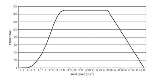
Wind turbines converts kinetic energy present in the wind into electric power. The wind speed varies continuously as a function of time, height geographical location and season. Due to the fluctuating nature of wind speed there is practical limitation for using wind as a source for power generation (Ackerman, 2005). The wind speed fluctuations which occur in the sub-second to minute range are called as turbulent peak. The diurnal peak depends on daily wind speed variations and the synoptic peak depends on changing weather patterns due to seasonal cycles. The turbulent peak may affect the power quality of wind power production. The impact of turbulence on power quality depends very much on the type of turbine technology used. The variable speed wind turbines may absorb short term power variations caused due to wind speed variation by the immediate storage of energy in the rotating masses of the wind turbine drive train. Due to which their power output is smoother than that of strongly grid coupled turbines. Diurnal and synoptic peaks, however, may affect the long term balancing of the power system (Ackerman, 2005), (Shingare, 2014). Due to fluctuations in wind speed, power generated by the turbine also fluctuates. Figure 5 shows the relation between wind speed variation (IMD, 2015) and power generated by a single turbine manufactured by a leading manufacturer.
Fig. 5 Wind speed and power generated by a single wind turbine (IMD, 2015)
The literature shows that, in order to reduce the impact of wind speed on power generations and sudden power fluctuations following steps are suitable:
1. Modification in power curve: Some wind turbine manufacturers offer wind turbines with special type of power curve as shown in Fig.6.
Fig. 6 Modified Power curve (Ackerman, 2005)
In these turbines, instead of a sudden cut off, power generation is reduced step by step with increasing wind speed above cutoff speed (Ackerman, 2005). This certainly reduces the possible negative impacts that very high wind speeds can have on power system operation.
2. Aggregation of wind turbines: The aggregation of wind turbines provides a positive effect on power system operation and power quality (Ackerman, 2005). By increasing the number of wind turbines in the wind farm reduces the impact of the turbulent peak as gusts do not hit all the wind turbines at the same time. Thus there will be less power variation in the resultant output power. Under ideal conditions, the relation between percentage variation of power output and the number of wind generators is given using Eq. (2) (Ackerman, 2005).
where n is the number of wind turbine generators.
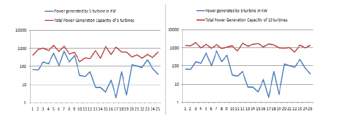
Thus in order to achieve a significant smoothing effect, the number of wind turbines within a wind farm does not need to be very large. Figure 7 shows the resultant power variation with a change in wind speed (IMD, 2015), during the aggregation of 5 and 10 wind turbines. It is observed that the power fluctuation during the aggregation of ten wind turbines is less than that of five. The resultant power output of 10 wind turbines is smoother as compared to 5 turbines.
Fig. 7 Total Power generated by aggregation of 5 and 10 Wind Turbines respectively (IMD, 2015)
3. The distribution of wind farms over a wider geographical area: It reduces the impact of the diurnal and synoptic peak significantly as changing weather patterns do not affect all wind turbines at the same time. If changing weather patterns move over a larger terrain, maximum up and down ramp rates are much smaller for aggregated power output from a very large single wind farm.
5.3 Low Voltage Ride Through (LVRT)
Low Voltage Ride through (LVRT) or Fault Ride Through (FRT) is defined in the grid codes of different countries. Grid codes are the rules and regulations set by power system operators which need to be obeyed by all power generators in order to get connected with the power grid. In case of wind turbine generators, grid codes ensure power system operators to extend wind generator’s grid connection during the grid faults(Gehlhaar, 2010). Low Voltage Ride Through (LVRT) describes the grid connection requirement of the wind turbine generating plants when the grid voltage gets temporarily reduced due to a fault or sudden load change (Leao, et al, 2011). During the penetration of wind power, a mismatch is produced between the generated active power and active power delivered to the grid. LVRT requirement helps in the management of this mismatch at the point of common coupling (PCC).
In the presence of grid voltage dips, the wind power plants are required to stay connected to the grid and remain operational thereby supporting the grid with reactive power (Malia, et al, 2013). The LVRT requirements guarantee the connection and support of generating plants to the grid during voltage drops. During the voltage drops, the generating plants support the grid by feeding reactive current into network thereby raising the voltage. After the fault clearance, the active power output is increased again to the value prior to the occurrence of the fault, within a specified period of time (Dirksen, 2013). LVRT helps in maintaining voltage stability of a grid connected wind power system by preventing premature tripping of numerous wind generators thus reduces the risk of voltage collapse (Malia, et al, 2013).
Conclusion
In power system most of the complexities occur due to the interconnections of different types of power generators, transmission line, transformer, and varying nature of load. Therefore, it is challenging to maintain reliable and healthy power system while integrating renewable energy sources with power grid. In this paper we discussed power quality, power quality challenges, it’s parameters, various power quality customers, and the cost of poor power quality. Further, we discussed various solutions to address the power quality challenges by incorporating the various methods along with technological advances.
Acknowledgement
This work was partially supported by Bharati Vidyapeeth College of Engineering, Navi Mumbai. We are thankful to our colleagues for their support and encouragement.
References
G. Shafiullah, M. Amanullah, A. ShawkatAli, P. Wolfs P. (February 2013), Smart Grid for a Sustainable Future, Smart Grid and Renewable Energy, Scientfic Research, pp. 23-34. Sandhu M., Thakur T. (2014). Issues, Challenges, Causes, Impacts and Utilization of Renewable Energy Sources Grid Integration. International Journal of Engineering Research and Applications, ISSN : 2248-9622, Vol. 4, Issue 3( Version 1), pp. 636-643. J. Enslin (July 2010), Network impacts of high pen-etration of photovoltaic solar power systems, IEEE Power and Energy Society General Meeting, pp.1-5. N. Roy, M. Mahmud, Pota H. (Aug 2011). Impact of high wind penetration on the voltage profile of distribution systems North American Power Symposium (NAPS), pp.11-6. T. Ackermann, (2005). A book on: Wind Power in Power Systems, Wiley Publication, England, pp. 97-112,169-182. Darrow K., Hedman B. (December 2005). The Role of Distributed Generation in Power Quality and Reliability, Final Report for New York State Energy Research and Development Authority, 17 Columbia Circle, Albany, New York 12203-6399, pp.1-118. A.Velayutham, (January 2015), Expert talk on Power Quality (PQ) Issues in smart Grid and Renewable Energy Soures, Ex Member,MERC, at SGRES, CPRI, Bangalore. M. Singh, Khadkikar V., A. Chandra, . Varma R (January 2011). Grid Interconnection of Renewable Energy Sources at the Distribution Level With Power-Quality Improvement Features, IEEE Transaction on Power Delivery, VOL. 26, NO. 1, pp. 307-315. C. Tejavoth, M. Trishulapani, V. Rao, Y. Rambabu (July 2013). Power Quality Improvement for Grid Connected Wind Energy System using STATCOM-Control Scheme, IOSR Journal of Engineering (IOSRJEN), ISSN: 2278-8719, Vol. 3, Issue 7, ||V6 || PP 51-57. A. Almeida, L. Moreira, J. Delgado (2013), Power Quality Problems and New Solutions, ISR Department of Electrical and Computer Engineering University of Coimbra, PloII, 3030-290 Coimbra (Portugal), Accessed on August 2014, pp. 1-9. Shingare Prashant, (May 2014), Wind Turbine Control Systems Theory and Practices, Invited Technical Talk at one week workshop on, Passivity Based Control New Vistas, held at VJTI, Mumbai during 19-23 May 2014. W. Deng, W. Pei (April 2008), Impact and improvement of distributed generation on voltage quality in micro-grid, Third International Conference on Electric Utility Deregulation and Restructuring and Power Technologies, pp.1737-1741. E. Hayden, (2013) Introduction to microgrids, Securicon, LLC, 5400 Shawnee Road, Suite 206, Alexandria, Virginia 22312 USA, pp.1-13. Gungor V., Hancke G., Buccella C., (Nov 2011). Smart Grid Technologies: Communication Technologies and Standards, IEEE Trnsaction on Industrail Informatics, VOL. 7, NO. 4, pp.529-539. NIST (2010), NIST Framework and Roadmap for Smart Grid Interoperability Standards, Release 1.0. U.S. Department of Commerce, Gary Locke, Secretary, pp.1-145. Daily wind data, Agricultural Meteorology Division, India Meteorological Department (IMD), June 2015, www. imdagrimet.gov.in Leao R.P.S, Almada J.B., P.A. Souza, R.J. Cardoso, R.F. Sampaio, F.K.A. Lima, Silveira J.G. and Formiga L.E.P. (2011), The Implementation of the Low Voltage Ride-Through Curve on the Protection System of a Wind Power Plant, Inter-national Conference on Renewable Energies and Power Quality (ICREPQ11), pp. 1-6. Malia S., S. Jamesb, I. Tankb (2013), Improving low voltage ride-through capabilities for grid connected wind turbine generator, 4th International Conference on Advances in Energy Research 2013, Elsevier, ScienceDirect, Energy Procedia 54, pp. 530 – 540. J. Dirksen, (2013), LVRT: Low Voltage Ride-Through, DEWI Magazin No. 43, August 2013, pp. 56-60. Gehlhaar T, (2010), Grid Code Compliance beyond simple LVRT, Germanischer Lloyd Industrial Services, GmbH, Competence Centre Renewable Certification, Hamburg, Germany [Online], pp 1-3.
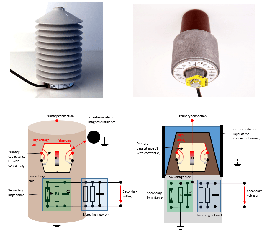
A reliable energy supply has meanwhile become an important location factor for many companies. While power failures and voltage fluctuations were among the most important parameters of supply quality in the past, voltage transients and voltage harmonics are becoming more and more important. This is mainly due to the increasing number of non-linear loads and many decentral renewable energy sources. In order to guarantee uniform standards for electrical energy supply in Europe, the minimum requirements for voltage quality are defined in a European standard. This is EN 50160, which is entitled “Voltage Characteristics in Public Distribution Systems”. This standard is to be understood as a product standard for electrical energy and for this reason is also used as a valid product standard in electricity supply contracts.
In February 2014 the Federal Court of Justice in Germany made it unequivocally clear that electricity is also subject to the Product Liability Act. The distribution network operator is thus liable for damage to electrical consumers that can be traced back to poor voltage quality on the part of the distribution network operator. For this reason, many measuring device manufacturers now offer measuring devices that prepare automated quality reports in accordance with EN 50160. Digital billing meters are also increasingly offering power quality functions in accordance with EN 50160. While the measuring devices can process the voltage directly in the low voltage range, we rely on voltage transformers or voltage sensors in the medium voltage range. The voltage quality is usually measured on older already existing systems. However, the built-in voltage transformers usually do not give any indication of the transmission behaviour at higher frequencies on the rating plate.
The devices are only specified for the 50 Hz fundamental frequency of the network. However, measurements according to EN 50160 require a frequency range of up to 2 kHz. We want to investigate the question of whether the existing devices are suitable for measurements up to 2 kHz.
Almost without exception, the built-in voltage transformers are inductive transformers that work according to the transformer principle.
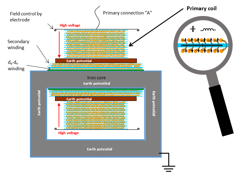
Figure 1:Model of the active part of a MV voltage transformer
In detail, the primary coil not only consists of inductive copper windings, but capacities also result from the individual layers isolated from one another. The capacities between the individual turns also contribute to the total capacitance of the primary coil. This results in a resonant circuit made up of inductance, capacitance and ohmic resistance, which must also have a corresponding resonance frequency.
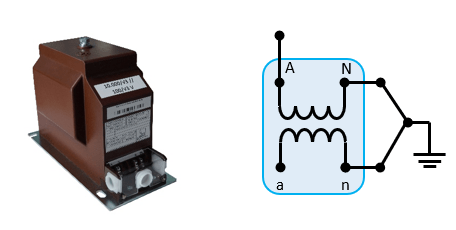
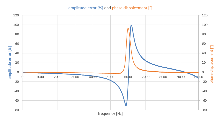
In order to find this resonance frequency, a commercially available 10 kV voltage transformer is now tested with the “frequency sweep method” with 6,400 measuring points up to 10 kHz.
Figure 2: Inductive single pole 10 kV voltage transformer (VTS12M11-T)
We found it!
Figure 3: Amplitude error and phase displacement of a 10 kV voltage transformer
A resonance point can be seen at approx. 6 kHz. While the voltage transformer transmits the primary signal acceptably up to approx. 5 kHz, an amplitude error of approx. 100% and a phase error of 87 ° results at approx. 6 kHz. A reliable PQ analysis up to 9 kHz can therefore not be carried out with this voltage transformer.
Despite the normatively regulated voltage levels, every instrument transformer manufacturer has a large number of different voltage transformers with different primary coils in order to be able to meet the most diverse secondary configurations by the customer. These voltage transformers have already been delivered and installed in measuring fields. The manufacturer can only carry out a rough calculation of the first resonance point in connection with the archived production documents. However, the resonance point measured in practice can often deviate from the calculation result by a few kHz. It is therefore very difficult for instrument transformer manufacturers to make reliable statements for devices that have already been delivered.
A contribution from the technical and scientific organization CIGRE / CIRED offers the measuring point operators good support. A guideline for power quality measurements was published here, which provides a meaningful table with regard to the frequency transmission behaviour of voltage transformers.
Figure 4:Suitability of inductive transformers for harmonic measurements (Source: CIGRE / CIRED Guidelines for Power Quality Monitoring WG C4.112 TECHNICAL BROCHURE 596)
It can be seen that 10 kV voltage transformers up to the 50th harmonic (2.5 kHz) can generally be used for PQ measurements. This statement is consistent with our measurement result in Figure 3.
In the 20 kV range, however, according to the table, devices have already been found that do not provide any reliable measured values on the secondary side from the 21st harmonic upwards. In the 30 kV range, there is even a general approval up to the 7th harmonic. We state that only 10 kV voltage transformers can be used in existing systems for reliable EN 50160 measurements. In the voltage levels 20 and 30 kV, information must be provided by the instrument transformer manufacturer.
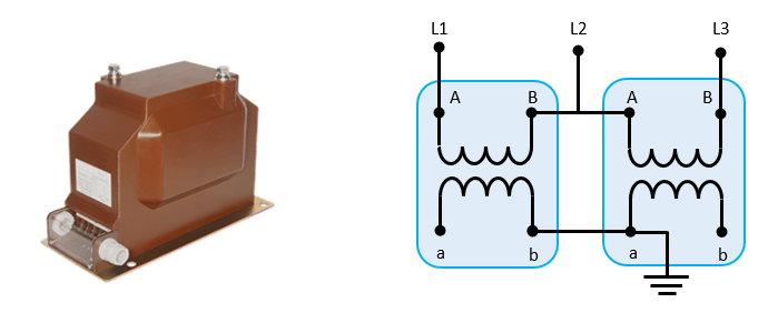
The voltage transformers examined here are exclusively single-pole devices. Two-pole voltage transformers, which can still be found in older existing installations in medium voltage grids, cannot be used for the analysis of harmonics. This is due to the voltage measurement between the conductors.
Figure 5:Two-pole voltage transformer with Aron circuit (two-wattmeter circuit)
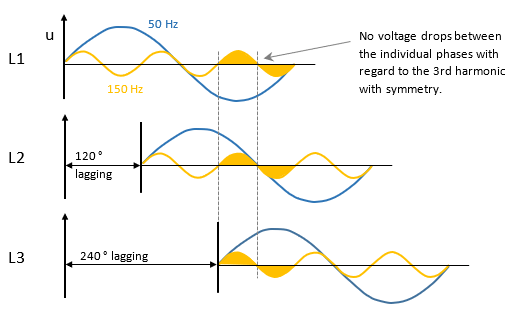
Despite the 120 ° phase shift of the 50 Hz conductor voltages, the amplitude values of the superimposed 3rd harmonic are not offset and thus cannot generate a voltage difference between the conductors. This generally applies to all harmonics divisible by 3.
Thus, the THDu obtained by the two-wattmeter circuit is reduced by the values of the voltage harmonics divisible by three (3, 6, 9,…).
Figure 6:Representation of the 50 Hz fundamental oscillation and the 3rd harmonic
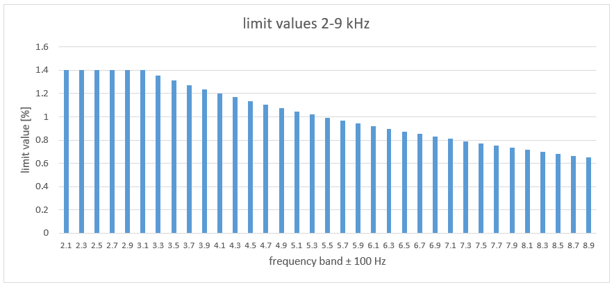
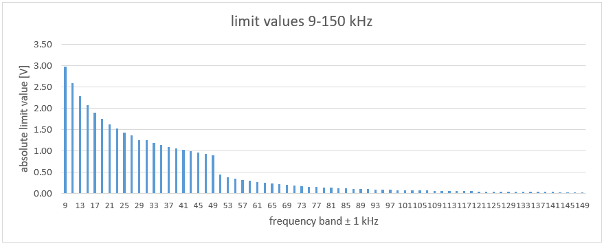
Furthermore, the question arises whether measurements up to 2 kHz are still sufficient. The current IEC 61000-2-2 (Environment – Compatibility levels for low-frequency conducted disturbances and signaling in public low-voltage power supply systems) already specifies limit values for voltages up to 150 kHz.
Figure 7:Limits for voltage harmonics from 2 to 9 kHz acc. to IEC 61000-2-2
Figure 8:Limits for voltage harmonics from 9 to 150 kHz
The EN 50160 cited in electricity supply contracts has been updated in 2020, but limit values beyond 2 kHz have not yet been bindingly defined. Thus, a voltage measurement up to 2 kHz is sufficient for determining the quality of the electrical energy. However, PQ measurements up to 9 kHz are already required for the grid connection of feed-in plants.
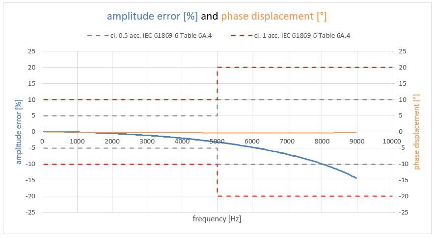
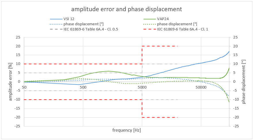
MBS AG therefore offers frequency-optimised voltage transformers up to 24 kV for the measurement range up to 9 kHz. The accuracy requirement for these transformers is defined in IEC 61869-6. The amplitude and phase errors are as follows.
Figure 9:Frequency-optimised 24 kV voltage transformer VTS24M32-T from MBS AG (amplitude error and phase displacement)
The transformer maintains class 0.5 up to approx. 8 kHz. From 8 kHz, class 1 is still clearly maintained. These voltage transformers thus enable reliable PQ measurement up to 9 kHz and, like all other medium-voltage transformers from MBS AG, are also SF6-free.
Many experts are already assuming that PQ measurements up to 150 kHz will also be carried out in the medium voltage in the future. Even some of the current mobile PQ analysers already measure up to at least 150 kHz, which may well be necessary for comprehensive interference analysis.
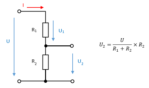
With inductive voltage transformers, the range up to 150 kHz is not technically feasible. With 24 kV devices, the first resonance point can only be pushed into the range of 10 to 20 kHz. Voltage sensors based on the voltage divider principle offer an alternative. As a reminder, the basic principle is shown here once again.
Figure 10:Principle of the voltage divider
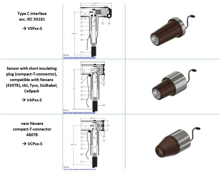
Already today, voltage sensors are mainly installed in existing local network stations that require an additional voltage measurement on the medium voltage side. Measuring fields with conventional inductive voltage transformers can only be retrofitted in rare cases for reasons of space. A proven method is to mount sensors in so-called T-connectors. This solution is space-saving and the installation is carried out by trained personnel within a reasonable time window. While the cone of the symmetrical connector is standardised according to IEC 50181, the cone of the compact T-connector has slightly different dimensions depending on the manufacturer. However, due to its patented design, the VAPxx-S voltage sensor intended for the compact T-connector can be used in the slightly different T-connectors of all well-known manufacturers without having to fear partial discharges. For the new type of compact T-connector from Nexans (480 TB), there is already also the matching sensor with the VCPxx-S.
Figure 11: Currently available connector types with the corresponding voltage sensors for the 12 and 24 kV insulation series
The sensors shown in Figure 10 can be used up to a maximum of 24 kV. A 36 kV version is already planned.
For air-insulated switchgear or measuring fields, MBS AG has a sensor that is already being used in new systems as well as for retrofitting.
Figure 12: Voltage sensor VSIxx-S for air-insulated switchgears
While the accuracy class at 50 Hz is noted on each sensor rating plate and is thus the responsibility of the manufacturer, manufacturers often do not provide protocols or reliable statements for measurements beyond 50 Hz. In the market, end users often hear the prejudice that ohmic dividers can generally transmit harmonics very well. This will be investigated in the following.
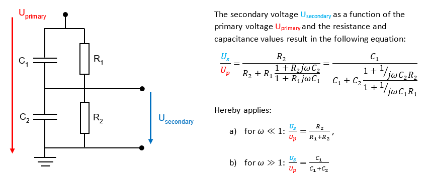
A resistive divider basically consists of two almost ohmic resistors, but these resistors always have parasitic inductive and capacitive components. A capacitance also forms around the high-voltage resistor, so that the technical literature does not speak of ohmic dividers, but of ohmic-capacitive dividers.
Figure 13:Schematic diagrams of an air-insulated voltage sensor (VSIxx-S) and a voltage sensor as termination insert of the T-connector (VAPxx-S)
A simplified equivalent circuit can be derived from the figure above.
Figure 14:Simplified equivalent circuit diagram of the RC divider
For the frequency independence of Us/Up, the following condition applies to the above equation.
R1C1 = R2C2
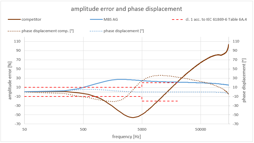
The question now arises whether ohmic-capacitive sensors in the medium voltage can be used for PQ measurements without further ado. In the following figure, a competitor’s and MBS’s own 50 Hz sensor have been measured from 50 to 150 kHz with respect to amplitude and phase errors.
The question now arises whether ohmic-capacitive sensors in the medium voltage can be used for PQ measurements without further ado. In the following figure, a competitor’s and MBS’s own 50 Hz sensor have been measured from 50 to 150 kHz with respect to amplitude and phase errors.
Figure 15:Amplitude error and phase displacement of two 50 Hz voltage sensors (X-axis logarithmically scaled)
Both sensors are outside the minimum requirements of class 1 for PQ measurements according to IEC 61869-6. For optimum transmission behaviour, the alignment network must also be optimized for higher frequencies.
MBS AG can currently provide voltage sensors for T-connectors and for air-insulated systems with optimized transmission behaviour up to 150 kHz.
For PQ measurements, frequency-optimized sensors are absolutely necessary in order to comply with the minimum requirement (class 1 according to IEC 61869-6). Transfer curves from current customer projects are shown in the following figures.
Figure 16:Amplitude error and phase displacement of the frequency-optimized sensors VAP and VSI (X axis logarithmically scaled)
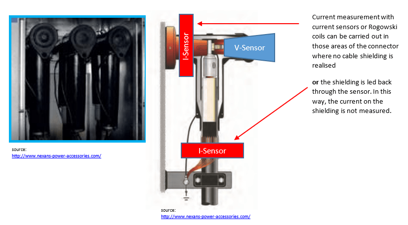
The voltage sensors are usually installed with corresponding current sensors. Unlike conventional current transformers, a voltage signal is output on the secondary side. However, broadband Rogowski coils can also be used.
Figure 17:Current and voltage measurement on the medium voltage side at MV cable feeders
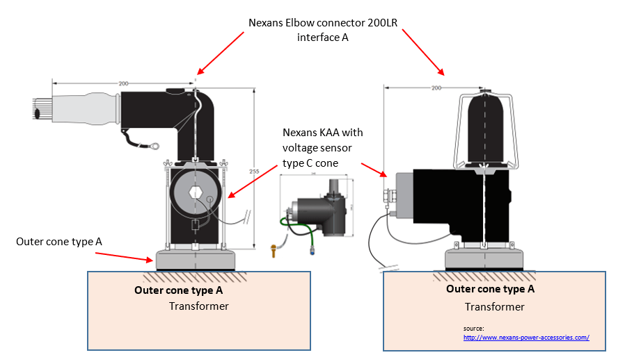
Various cable connector manufacturers also offer adapters for the external cone A. Thus, voltage measurements can be realised directly at the transformers in a space-saving way.
Figure 18: Nexans KAA with voltage sensor + Elbow connector 200LR with interface A
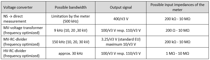
When selecting the measuring device, it should be noted that the voltage sensors addressed here can provide a maximum of 10/√3 volts on the secondary side. In Germany, the standard 3.25/√3 V has already become established. For current sensors, 225 or 333 mV are usually used.
Here, a problem often arises for the utility company when purchasing a mobile power quality analyser. In contrast to the traditional inductive voltage transformers with 100/√3 V, the voltage sensors only give a small signal up to a maximum of 10/√3 V. In the low-voltage range the voltage is measured directly. Frequency-optimised high-voltage transformers, which are designed also as RC dividers, usually provide 100/√3 V like conventional voltage transformers. This results in a wide variety of secondary voltages in the environment of energy supply companies.
Figure 19: Table. Measuring voltages on the voltage side of a utility
In order to be able to guarantee sufficient resolution and accuracy, a mobile PQ measuring device should be designed for these different measuring voltages. The only mobile measuring device that currently meets these requirements is the PQA 8000H-P from NEO MESSTECHNIK. It has switchable voltage inputs for 600 Vpeak and 10 or 20 Vpeak. With this option, it is possible for the utility company to carry out high-quality PQ measurements in the different voltage levels.
Figure 20: Mobile PQ meter PQA8000H-P with switchable voltage inputs especially for utility companies
FFT analysis up to 500 kHz (voltage & current) in 2 kHz bands (according to international standard IEC61000-4-30)Scope View with 1 MS/s
4x voltage measurements / up to 8x current measurements
Display and recording of the digital PLC data stream
Two voltage measuring ranges (switchable) of 600 Vp and 10 Vp
All voltage inputs isolated (CAT III 1000 V / CAT IV 600 V)
Power supply of the current sensors directly from the unit
The input impedance of the voltage channels is 10 MOhm || 2 pF. Conventional voltage transformers in medium voltage are specified in terms of class accuracy with a burden power in VA. Values between 5 and 20 VA are common. The class noted on the rating plate applies to 25 to 100 % of this power. The power requirement of the mobile PQ unit is vanishingly small at the usual secondary output voltage of 100/√3 V.
The measuring device can therefore be operated in parallel to the connected measuring devices without affecting the accuracy.
The situation is different with the sensors in the medium and high voltage. Here, the RC dividers are precisely calibrated to the load resistance. In the high voltage, therefore, an extra terminal is often designed for the PQ measuring device. In medium voltage, the sensor must be precisely matched to the measuring device. However, measuring devices can also be operated in parallel here. By using parallel additional resistors, the PQ meter can be simulated when not in use.
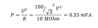
Figure 21: Calculation of the total burden seen by the voltage sensor
When using several measuring devices in different measuring stations, a convenient connection to the ENA SCADA system is possible.
Figure 22: SCADA System ENA SCADA for the control room
It can be stated that by using ohmic-capacitive voltage sensors in the medium voltage in connection with a switchable mobile PQ analyser, measurements up to 150 kHz can also be carried out. With RC dividers in the high voltage, a measuring range of up to 30 kHz can currently be covered. From a technical point of view, there is no obstacle to adopting the limit values from the current IEC 61000-2-2 into EN 50160 for low and medium voltage. Only in the high voltage level the bandwidth is limited to 30 kHz.
Published by Omar H. Abdalla, Fellow Egyptian Society of Engineers, Life Senior Member IEEE.
Prof. O. H. Abdalla is with the Department of Electrical Power and Machines Engineering, Faculty of Engineering, 1 Sherief Street, P.O. Technology, P.C. 11792, Helwan, Cairo, Egypt. (e-mail: ohabdalla@ieee.org).
Conference Paper: Keynote Lecture (KL-REN-5), International Conference on New Energy and Environmental Engineering (ICNEEE), Future University, Cairo, Egypt, 11-14 April, 2016.
Abstract
The objective of this paper is to provide basic information on the technical design specifications, criteria, technical terms and equipment parameters required to connect PV systems to the distribution networks in Egypt. Successful connection of a PV system should satisfy requirements of both the ssPV Code and Electricity Distribution Code. The ssPV Code specifies the special requirements for the connection of small-scale PV systems to the Low Voltage (LV) distribution network. The Electricity Distribution Code (EDC) sets out the rules and procedures to regulate technical and legal relationship between distribution utilities and users of the distribution networks. The aim is to maintain optimal operation, safety and reliability of the power system. The technical specifications including permitted voltage and frequency variations in addition to power quality measures such as limits of harmonic distortion, phase unbalance, and flickers. Small-scale PV system operational limits, capability requirements, power factor, safety, protection, synchronization, etc. will be explained and discussed. In addition, the roles stipulated in the EDC for connecting distributed generating units to the distribution networks are briefly presented.
Index Terms—Distribution networks, Photovoltaic systems, PV integration, Distribution code, PV connection code.
I. INTRODUCTION
There has been a continuous increase in the share of the renewable resources in generating the required electricity to cope with increasing demand. Future electricity generation plans countries around the world expect more contribution of renewable energies in the electricity generation mix. Some utilities set a target of 20% renewable energy of total required energy by 2020. Others expect 50% by 2050. Among various renewable energies, wind and solar are the most promising resources and proved to be efficient in real applications at decreasing competitive kWh costs.
The increasing ratio of renewable energy sources to be connected to electric power systems has resulted in technical issues related to power quality, capacity, safety, protection, synchronization, etc. Electricity utilities and regulators have issued regulation roles for connecting renewable energy sources to power grids at distribution level and transmission level.
An overview of recent grid codes for PV power integration is presented in [1]. It provides a survey of grid codes, regulations and requirements for connecting PV systems to LV and MV networks, including power quality concerns and anti-islanding issues. A guide to PV interconnection issues [2] has been developed by the Interstate Renewable Energy Council, North Carolina Solar Center, USA. Interconnection issues cover all steps for connecting a small scale renewable energy system to the utility network, including technical, contractual, and rates and metering issues. German codes for connecting PV systems to medium voltage power grid are described in [3]. A comparison of Germany’s and California’s interconnection processes for PV systems is discussed in [4]. The IET has developed the Standards: “Code of Practice for Grid Connected Solar Photovoltaic Systems [5]. The National Energy Regulator of South Africa has approved the “Grid Connection Code for Renewable Power Plants Connected to the Electricity Transmission System or the Distribution System” [6].
This paper concerns with technical design specifications and criteria, technical terms and equipment parameters required to connect small-scale PV systems to the distribution networks in Egypt. Successful connection of a PV system should satisfy requirements of both the ssPV Code [7] and the Electricity Distribution Code [8].
The ssPV Code specifies the special requirements for the connection of small-scale PV systems to the Low Voltage (LV) distribution network. Although the ssPV code is all complementary documents that entail obligatory provisions for customers seeking ssPV installations [7], the customer should also satisfy the requirements of the Distribution Code. Technical terms of these codes should be clearly understandable by all parties to correctly implement the rules and procedures described in the codes.
The Electricity Distribution Code is a document that contains a set of rules and procedures to regulate technical and legal relationship between a Distribution System Operator (DSO) and users of the distribution network. The objective is to establish the obligations and responsibilities of each party; i.e. the DSO and all network users; namely, subscribers, distributed electricity production units, etc. This will lead to maintain optimal operation, safety and reliability of the power system.
The technical specifications of integrating small-scale PV systems to the distribution networks include permitted voltage and frequency variations in addition to power quality measures such as limits of harmonic distortion, phase unbalance, and flickers. PV systems operational limits, capability requirements, power factor, safety, synchronization, protection, etc. will be explained and discussed.
Section II presents a brief review of power quality terms and criteria referred to in the ssPV Code. Section III describes the technical requirements and criteria for connecting small scale PV systems to the low voltage distribution networks in Egypt. Section IV summarizes the technical requirements and criteria for connecting distributed generations to distribution networks as stipulated in the Electricity Distribution Code.
II. REVIEW OF POWER QUALITY CRITERIA
This section reviews briefly power quality issues related to both the Distribution Code and the small-scale PV Code in order to understand respective terms in the codes. Definitions, mathematical description, causes and impacts of various parameters are explained.
A. Voltage Flicker
If a load such as an arc furnace causes voltage variations at the PCC with spectral characteristics in the range of a fraction of one Hz and about one third of the system frequency, this effect is known as voltage flicker. It is a characteristic where a high frequency (𝜔𝑜) sinusoid is modulated by a low frequency sinusoid (𝜔𝑓). In mathematical form,
Intensity of flicker is given by,
𝑆𝑠𝑐𝑓 = short-circuit MVA at the electrode tip 𝑆𝑠𝑐 = short-circuit MVA at the PCC
The IEC has developed a flicker meter which measures flickers in terms of fluctuating voltage magnitude and its corresponding frequency of fluctuations. It uses a software technique to convert flicker voltage fluctuations into the following two statistical quantities:
Short-term flicker severity (PST)
Long-term flicker severity (PLT)
The flicker meter takes measurements automatically at ten minutes intervals. The short-term flicker severity is calculated every 10 minutes. The indicator PST having a value of 1 represents the level of visual severity at which 50% of people would perceive flicker in a 60 W incandescent bulb. The long-term flicker severity (PLT) is a combination of 12 PST values.
B. Voltage Unbalance
A 3-Ph power system is called Balanced if the 3-Ph voltages (& currents) have the same amplitude, and are phase shifted by 120o with respect to each other. If either or both of these two conditions are not met, the system is called Unbalanced.
The relation between the symmetrical components (V0, V1, V2) and the phase components (VA, AB, VC) is,
V0, V1 and V2 are the zero-, positive-, and negative-sequence components, respectively. According to the EN-50160 and IEC-61000-3-x, standards the voltage unbalance (V2U) is defined as,
The standards stipulate the following voltage unbalance limits:
These values are measured as 10-minute average value with an instantaneous maximum of 4%.
Causes of unbalance include generators, transformers, unbalanced impedances of long, non-transposed low voltage lines, unbalanced load currents, 1-phase loads on 3-phase systems, etc. Unbalance can adversely affect equipment such as motors and transformers by increase heating and reduce efficiency.
C. Harmonics
Linear loads such as incandescent lighting and heating draw currents proportional to applied voltages, whilst non-linear loads computers and adjustable speed drives draw currents during a part of the voltage cycle. The currents of nonlinear loads contains odd harmonics (3rd, 5th, 7th, etc.). Harmonic currents interact with source currents, leading to voltage harmonics. These harmonic components are superimposed on the fundamental voltage component resulting in a distorted voltage wave, which has the following Fourier form:
Where
Having determined the fundamental U1 and harmonic components (U2, U3, U4, etc.), we can calculate the Total Harmonic Distortion (THD),
Harmonic currents can cause problems such as equipment heating, false tripping of circuit breakers, neutral line overloading, increased skin effect, etc. Therefore, electricity codes stipulate limitations on THD in networks.
III. SMALL-SCALE PV CONNECTION CODE
A. General Design Requirements
The ssPV Code [7] specifies the technical requirements and criteria for connecting small scale PV systems to the low voltage distribution networks in Egypt. The small scale PV system is defined in practice as a PV electric energy generation source rated at up to 500 kW including the PV panels, converters, control devices, and protection gears within a customer’s network that operates in synchronism with the 3-phase LV distribution networks.
The ssPV system shall be type approved. Design qualification and type approval of PV modules are based on IEC-61215 / IEC 61649 Standards. The maximum size of the ssPV system is limited by the rating of the CB at the supply point on the premises, and the allowable voltage range at the LV side of the MV/LV transformer and the voltage at the farthest point of the feeder.
The technical requirements and criteria stipulated in the ssPV code are summarized in the following subsections.
B. Power Quality Requirements
The quality of electric power supplied at the PCC is governed by relevant practices and standards. The total flicker severity at the PCC, including the ssPV system and both existing and future loads, shall not exceed the following levels (for LV and MV):
The THD of the current produced from the ssPV system at rated output shall limited to be < 5%, while the individual harmonic components are listed in Table I, in accordance to the IEC 61727-2004 Standard.
TABLE I: LIMITS OF CURRENT HARMONIC DISTORTION AT THE PCC
C. Power Factor
Although, the ssPV Code prevents injection of reactive power from the PV system to the distribution network, it allows the customer to draw power at 0.9 pf lag limit (unless other pf is agreed).
D. Direct Current Injection
The limit of direct current (d.c.) injection into the network shall not exceed 0.5% of the rated a.c. ssPV current supplied at the PCC. If this limit is violated, the inverter must disconnect within 500 ms.
E. Synchronization
The ssPV system shall be synchronized to the network, through the static inverter after satisfying the following conditions:
Frequency difference ≤ 0.3 Hz,
Voltage difference ≤ 5%, and
Phase angle difference ≤ 20°.
F. Safety and Protection
For safety and protection of the ssPV system, the code specifies the conditions of disconnection from the network as follows:
If the voltage (V) of the network violates the limits as listed in Table II,
If the frequency (F) of the network violates the allowable operating limits as listed in Table III,
Loss-of-grid conditions, or
If the direct current injection exceeds the limit (0.5%).
TABLE II: VOLTAGE RANGES AT THE PCC AND MAXIMUM TRIPPING TIMES
TABLE III: FREQUENCY RANGES OF THE NETWORK AND MAXIMUM TRIPPING TIMES
For short-circuit protection, the ssPV shall comply with the IEC 60364-7-712 Standard titled “Electrical Installations of Buildings”. It concerns with the requirements for special installations or locations of solar PV power supply systems.
G. Switching Arrangement
Switching arrangement for disconnecting the ssPV system from the network in abnormal conditions is described in detail in the code. The abnormal conditions include violation of the limits of network voltage or frequency as specified in Table II and Table III, respectively. At least two series disconnecting switches are required; one of them shall be an electromechanical switch, while the other may be embedded in the inverter. The objectives are to ensure personnel safety and to avoid equipment damage. In response to network recovery, the ssPV system shall not re-energize the network for 1 minute.
H. Islanding
To comply with the ssPV connection code requirements, unintended islanding condition shall be prevented. At least, one method of active islanding detection shall be used. Active methods introduce small perturbation to the system and monitor the response to determine if the PV and the network are still connected [9]. If this affects the system parameters within prescribed requirements, the active circuit will causes the inverter to cease delivery of power. The ssPV system shall comply with the requirements of IEC 62116 Standard which specifies testing procedure of islanding prevention methods for utility-interactive PV inverters. Experimental studies are presented in [10]. In response to network recovery after islanding, the ssPV system shall not re-energize the network for 1 minute.
I. ssPV Earthing
Earthing of the ssPV electrical installation system shall comply with the requirements of the SANS 10142-1: Code of Practice Wiring of Premises. The ssPV Code requires that the ssPV system be protected by an earth leakage unit separated from customer network earth leakage units. The ssPV system inverter shall be appropriately using an earth leakage circuit breaker capable of responding to d.c. fault currents.
J. Energy Metering Arrangements
Metering circuits and types are described in the ssPV code, including unidirectional and bi-directional, with single or separate meters.
IV. ELECTRICITY DISTRIBUTION CODE
The Electricity Distribution Code (EDC) has been issued and effective since March 2010 [8]. The aim of the EDC is to regulate the electricity distribution and connection to the subscribers in a safe and stable manner, in addition to regulate connecting the distributed generating units with distribution networks. The code consists of 14 chapters including objectives, validity, planning of assets, contracting, quality of supply, distributed (or scattered) generation, plans for dealing with emergencies, metering code, in addition to legal and other electricity distribution regulating issues. Our concern here is the technical requirements of connecting distributed generation as described in chapter 6 of the EDC.
A. Distributed Generation (DG)
Chapter 6 of the Distribution Code stipulates the roles for connecting the distributed generating units to the distribution networks. The roles are briefly described here. The licensed distributor is obliged to facilitate connection of the DG units and access to use the network provided that they are compliant with the code requirements including technical, environmental and safety. The DG provider is obliged to continue operating the connected units at 50 Hz and be within the allowable frequency limits defined in the Transmission Grid Code [11]. According to the IEEE Standard 1547 – 2003 [12], the following specifications should be considered:
The DG unit should not cause network voltage changes outside the allowable limits (± 5%)
The unit earthing should not affect the consistency of adjusting protection devices of earth faults.
The unit should not cause voltage fluctuations or flicker outside the allowable limits.
The unit should not allow injecting direct current higher than 0.5% of the total rated A.C. current, at the PCC.
In addition, the DG unit should pass all technical tests specified in the IEEE standard 1547 – 2003, including:
Performance during voltage transients
Synchronization
Protection from electromagnetic interference
Limits of direct current
Voltage harmonics
The negative-sequence voltage component due to the DG should not exceed 1% at the PCC. The use of the DG should not lead to increasing the THD at the PCC exceeding the limits listed in Table IV and Table V (IEEE 519 – 1992, Standard). The DG units should not cause inductive interference exceeding the limits stipulated in the IEEE Standard C37.90.2. In designing and operating the DG, the short-circuit limits listed in Table VI should not be exceeded.
TABLE IV: LIMITS OF VOLTAGE HARMONIC DISTORTION AT THE PCC
TABLE V: LIMITS OF CURRENT HARMONIC DISTORTION AT THE PCC
Notes: ISC = maximum short-circuit current at the PCC IL = maximum load current of the fundamental component at the PCC
TABLE VI: SHORT-CIRCUIT LIMITS AT THE PCC
V. CONCLUSION
The paper has presented the technical design specifications, criteria, technical terms and equipment parameters required to connect PV systems to the distribution networks in Egypt. The specifications, terms and parameters are extracted from the ssPV Code [7] and Electricity Distribution Code [8]. The presented technical specifications and criteria are useful for researchers, design engineers, and installations engineers working in the field of connecting small-scale PV systems into distribution networks. For successful connection of small-scale PV systems to distribution networks, it is recommended to read the full versions of the ssPV Code and the Electricity Distribution Code.
REFERENCES
[1] B. I. Craciun, T. Kerekes, D. Sera, and R. Teodorescu, “Overview of recent grid codes for PV power integration,” 13th International Optimization of Electrical and Electronic Equipment, OPTIM, Brasov, Romania, 24-26 May 2012, pp. 959-965. [2] C. Larsen, B. Brooks, and T. Starrs, “Connecting to the Grid – A Guide to PV Interconnection Issues,” 3rd ed., Interstate Renewable Energy Council, IREC, North Carolina Solar Center, USA, 2000, pp. 1-37. [3] E. Troester, “New German Codes for connecting PV systems to medium voltage power grid,” 2nd International Workshop on Concentrating Photovoltaic Power Plants: Optical Design, Production, Grid Connection, Dramstadt, Germany, 9-10 March, 2009, pp.1-4. [4] A. Tweedie and E. Doris, “Comparing Germany’s and California’s interconnection processes for PV systems,” National Renewable Energy Laboratory, NREL, Clorado, USA, July 2012, pp. 1-60. Available: http://www.nrel.gov/docs/fy11osti/51814.pdf [5] IET Standards, “Code of Practice for Grid Connected Solar Photovoltaic Systems,” IET, UK, 2014, pp.1-120. [6] Grid Connection Code for Renewable Power Plants (RPPs) Connected to the Electricity Transmission System (TS) or the Distribution System (DS) in South Africa, Version 2.6, National Energy Regulator of South Africa, NERSA, South Africa, 2012, pp. 1-61. [7] Technical Requirements for Connecting Small Scale PV (ssPV) Systems to Low Voltage Distribution Networks, ssPV Code, Egyptian Electric Utility and Consumer Protection and Regulatory Authority, EgyptEra, Cairo., Egypt, 2014, pp. 1-9. Available: http://www.egyptera.org [8] Electricity Distribution Code, Egyptian Electric Utility and Consumer Protection and Regulatory Authority, EgyptEra, Cairo., Egypt, 2010, pp. 1-29. Available: http://www.egyptera.org [9] W. Bower and M. Ropp, “Evaluation of islanding detection methods for utility-interactive inverters in photovoltaic systems,” Sandia National Laboratories, Tech. Rep. SAND2002-3591, New Mexico, CA, 2002. [10] F. Belloni, P. Groppelli, C. Chiappa, and C. Gandolfy, “Test of anti-islanding protections according to IEC 62166: an experimental feasibility assessment,” The 48th International Universities Power Engineering Conference, UPEC 2013, Dublin, UK, 2-5 Sept. 2001, Available: http://www.xplore.ieee.org [11] Transmission Grid Code, Egyptian Electricity Transmission Company, EETC, Cairo, Egypt, Available: http://www.eetc.net.eg/grid_code.html [12] IEEE Standard for Interconnecting Distributed Resources with Electric Power Systems, IEEE Std 1547™-2003, Standards Coordinating Committee 21, IEEE, June 2003, pp. 1-16.
Author
Omar H. Abdalla, Misfah 220kV Grid Station
Omar Hanafy Abdalla (M’76–SM’83–Life SM’2014) was born in Cairo, Egypt on 11 May, 1945. He received the Ph. D. degree in electrical engineering from the University of Liverpool, England, in 1979. Since B. Sc. graduation in 1967, he has been appointed in various positions in university teaching and research: Engineer 1967, Demonstrator 1970, Lecturer 1976, Associate Professor 1983, Professor 1987, Head of the Department of Electrical Power & Machines Engineering 1987, Vice-Dean for Postgraduate Studies and Research 1997, Dean of the Faculty of Engineering 2002, Professor Emeritus 2005-now. He has published over 120 papers and appointed as a Reviewer for many national and international periodicals and conferences. He is a member of the Editorial Board of the International Journal of Emerging Electrical Power System, and the Editorial Board of the Journal of Electrical Systems.
From January 2007 to February 2014, he was on leave from the University of Helwan; working (System Studies Advisor) with Oman Electricity Transmission Company, Muscat, Sultanate of Oman. He was involved in various technical activities and leading strategic planning and transmission system studies such as the Transmission Master Plan 2014-2030, Five Year Annual Transmission System Capability Statements, planning and design of new generation and bulk industrial load connections, HV grid-stations, transmission lines of 400kV, 220kV and 132kV levels, network expansions and reinforcements, Pre-Investment Appraisal Documents for new projects, etc. He was also involved in the technical studies and practical operation of the interconnection between Oman and the United Arab Emirates.
Prof. Omar H. Abdalla received the Encouraging Prize of the State in Engineering Sciences, 1984, the First Class Medal of Sciences and Arts, 1985, and Helwan University Appreciation Prize in Engineering Sciences and Technology, 2006/2007.
T.R. Ayodele, Department of Electrical Engineering, Tshwane University of Technology, Email: Ayodeletr@tut.ac.za,*
A.A. Jimoh, Department of Electrical Engineering, Tshwane University of Technology, Email: JimohAA@tut.ac.za
J.L Munda, Department of Electrical Engineering, Tshwane University of Technology, Email: MundaJL@tut.ac.za
J.T Agee, Department of Electrical Engineering, Tshwane University of Technology, Email: AgeeJT@tut.ac.za
*Corresponding Author; T.R. Ayodele, Department of Electrical Engineering, Tshwane University of Technology, Private Bag X680 Pretoria 0001, Staatsartillerie Road, Pretoria West, South Africa, +27735605380, Ayodeletr@tut.ac.za
INTERNATIONAL JOURNAL of RENEWABLE ENERGY RESEARCH T.R. Ayodele et al., Vol.2, No.4, 2012
Abstract
Wind Energy Conversion Systems (WECSs) exhibit variability in their output power as a result of change in their prime movers (wind speed).This introduces a new factor of uncertainty on the grid and poses a lot of challenges to the power system planners and the utility operators in terms of the power system grid integrity i.e. power system security, power system stability and power quality. This paper discusses the various challenges of wind power when integrated into the grid and identifies different mitigating strategies for its smooth integration. This paper therefore enables the specifications for mitigation/integration technologies to be appreciated and quantified.
Efforts are geared towards grid integration of renewable energy sources into a grid as a result of environmental concerns and the quest for energy security [1]. Among the renewable energy sources, wind energy stands out because of its technological maturity, good infrastructure and relative cost competitiveness [2]. At present, the wind power growth rate stands at 20% annually and it is predicted that 12% of the world’s electricity may come from wind power by the year 2020 [3].
However, grid integration of the Wind Energy Conversion System (WECS) can potentially affect the power system negatively due to the fluctuation in wind power. The WECS exhibits variability in its output power because of the stochastic nature of wind resources as a result of incessant changes in weather conditions. This intermittent and diffuse nature of the wind power introduces a new factor of uncertainty on the grid and may have a negative impact on the grid integrity i.e. the power quality, the system security and the system stability. The dynamics and the control of conventional generators in a power system vis-à-vis grid interaction are well understood and falls under the control capability of the utility operators. Wind energy is controlled by nature and this can have a repercussive effect on the power system. For wind generators to effectively replace the normal conventional generators, then, it must be able to provide the same ancillary services provided by the conventional power plant by controlling the nodal voltages, ensuring load following, maintaining grid frequency, and contributing to fault current. Wind power penetration is still low (20% maximum in Denmark); the ancillary services are majorly supported by the conventional power plants. When the penetration level is increased, the technical impact on the grid integrity may arise which needs to be well understood.
This, therefore, implies the need for certain technologies to enable smooth and proper integration of WECSs to the grid. As such the necessary specifications for such technologies need to be properly understood and quantified. This paper sets out to address this. It discusses the various challenges of WECSs when directly integrated into the grid and sets out to define the parameters and variables necessary for smooth integration through different mitigating strategies.
2. Impact of Wind Power on System Security
The security of a power system is regarded as the ability of the system to withstand disturbances without causing a breakdown of the power system [4]. For wind power generators to contribute to the security of a power system, they must have the ability to contribute to both the voltage and frequency control in stabilising the power system following a disturbance, they must be able to ramp up or down to avoid insecure power system operation, they must be able to ride through disturbances emanating from the power system, they must be able to avoid excess fault levels while still contributing to fault identification and clearance, and they should be able to operate in island mode when the supply from the grid is lost [5].
Wind power generation is often faced with difficulties with regards to reliability in terms of the generation, planning and scheduling of the supply of electricity [6]. There is always a lack of confidence by the utility operators in the system’s capability to meet peak demands. Although, no electricity system is 100 percent reliable, intermittent generation will increase the level of uncertainty and therefore also the reserve capacity band of the power system which in turn increases the generation costs. The effect is minimal at low penetration levels, but could be challenging at high penetration levels [7, 8]. Among these challenges are the effects on the power imbalance, reserve management, voltage control and system stability.
2.1 Power Imbalance
WECS generate electricity when wind speeds exceed a certain minimum and the WECS output depends on these wind speeds. Wind speeds cannot be predicted with high accuracy over daily periods, and the wind often fluctuates from minute to minute and hour to hour. Consequently, electric utility system planners and operators are concerned that variations in the output of WECS may increase the operating costs of the system [9]. This concern arises because the system must maintain a balance between the aggregate demand for electric power and the total power generated by all power plants feeding the system. The variability and the unpredictability of wind power can cause a power imbalance on the grid [7, 8, 10, 11]. Their output power may not be available to meet the demand when needed, while there could be an excess when the demand is low, thereby causing an upset on the grid. [12] reported a loss of 4000MW (58% of capacity) in Germany in December 2004 and a loss of 2000MW (83% of capacity) within 6 six hours in Denmark in January 2005 as a result of large changes in wind power output due to a forecasting error. A penalty cost is often attached to the deviation in the scheduled and actual energy delivered to the grid to cover the reliability aspect of intermittent generation [12].
In line with the above, several publications exist on the generation adequacy of a power system incorporating intermittent wind power. A method for capacity adequacy evaluation of power system containing wind energy, solar energy and energy storage was presented in [13]. Also, an approach to generating capacity reliability studies, using the autoregressive moving average (ARMA) time series was presented in [14]. The technique is used to illustrate the effect of adding increasing amount of wind capacity to conventional generating system using the Loss of Load Expectation (LOLE) and Loss of Energy Expectation (LOEE) indices. The generating capacity credit attributed to wind power is expressed in terms of peak loading-carrying capability at the criterion risk level. An assessment of the generation adequacy of the Irish system incorporating wind energy capacity was studied in [15] using the application of both the LOLE and Monte Carlo simulation. Further readings on the adequacy assessment of power systems consisting of intermittent wind generators can be found in [16-20].
2.2. Impact of Wind Power on Reserve Management
Electrical power is expensive to store. Hence, the power produced at the generating station must be consumed by the load. Therefore, there must be a power balance between all the generating plant and the load demand. Any imbalance would affect the frequency of the system which could lead to loss of synchronism in certain cases [21]. The accomplishment of a power balance between the load and the generating plants is more challenging in the case of wind power generation due to its unpredictable nature especially when the generating ratio is high. A system of high wind power integration would expand the reserve capacity due to the variability of the primary resources [22]. A conventional power plant is expected to provide for this variability. This has an effect on both the operational costs and the ancillary service costs of the power system. An extra reserve of 3-6% of the rated capacity of the wind plant is required in a 10% wind integration and 4-8% approximation for 20% wind integration [23]. In a United Kingdom study, an additional balancing cost due to 10% integration of wind power cost £40 million (£2/MWh) and £200 million per annum (£3/MWh) for 20% wind integration. A national grid assessment study on the impact of 30GW wind capacity integration by the year 2020 on the reserve capacity indicates that 30GW levels of wind generation will increase the short-term operating capacity to 10.5GW from the 2009 (4GW capacity) at an additional cost of about £418 million per annum. This translates to approximately £5.4/MWh of wind generation [24]. A summary of studies conducted by the U.S. or on behalf of the U.S. utility which provides valuable insight into the issue of wind power impacts on overall electric system operating costs can be found in [9].
2.3. Impact on the Power System Voltage Control
The nodal voltage distribution on a power system network must not be less than an acceptable limit. The reactive power contribution capability of a power plant determines its nodal voltage control. A conventional generator has a way of controlling the reactive power to ensure a proper voltage distribution at the different nodes of the network. Most WECS make use of induction generators which are not capable of injecting reactive power to the grid [21]. This often forms one of the limitations of wind power integration.
3. Impact of Wind Power on Power Quality
The degree of deviation from the normal sinusoidal voltage and current waveforms in power system network determines the quality of the power transmitted on the grid [25]. The liberation of the electricity market has resulted in power quality becoming an issue of focus in recent times. Power quality components of a power system comprise of flickers, harmonic distortions, voltage imbalance, voltage sag and voltage swells.
The level of tolerance of power quality depends on the kind of load installed by the customer, that is, how sensitive the load is. The occurrence and frequency of power quality problems depend on the strength of the network, type of consumer load fed by the network, electronic equipment utilised, geographical location of the area, length of the network, load behaviour, climate change and the operational practice of the utility operators [26].
Poor power quality could lead to losses on the grid, malfunctioning of the electrical equipment and even a loss of synchronism that could lead to network failure. Low power quality has negative consequences on the economic and social life of a modern society. A power quality survey conducted in Europe revealed an estimated loss of approximately 150B€ in a year [27], while an estimated loss of between 119b$-188b$ per annum was reported in the United States of America [26].
Variable speed wind generators, that is, WECS made of doubly fed induction generator (DFIG) and synchronous generator (SG), require power converters to achieve controllable grid integration. These converters are sources of harmonics especially in grids with low short circuit capacity. In addition, most wind resources are found very far from the city where access to strong grids is limited. The grid in this area is initially planned for unidirectional power flow. Wind power integration could have a negative impact on the steady state operation of these kinds of grids.
Fixed speed wind turbines produce power pulsation due to shear effects and tower shadows and this could result in a voltage fluctuation that could cause flickers on the grid [28]; however, the effects are reduced in variable speed wind generators.
There are certain standards in place to ensure uniform power quality measurement. These standards specify how a power quality measurement should be conducted and the level it should not exceed. The standards are IEEE 519-1992, IEC 61000-4-30 and EN50160. IEEE 519-1992 deals with the practices of and requirements for harmonic control in electrical power systems. It specifies the limits of harmonic voltage and current at the point of common connection between the end user and the distribution utilities. The standard requires the participation of both the utilities and the customers. IEC 61400 describes the adequate measurement methods for ensuring voltage and current quantities. It provides the aggregation periods and the measurement formulars. The EN50160 code is mostly adopted by European countries and it sets the standard level for different power quality components which should not be exceeded [29]. IEC issued a standard in 2001 (IEC 61400-21) for the measurement and assessment of the power quality in wind turbines. The standard defines power quality characteristics of wind turbines and proposes a measurement procedure [29]. Apart from the international standards, there are also various national grid codes in order to ensure quality power supply.
3.1. Harmonics
Harmonics can be injected both at the generation and the consumer end. At the consumer end, harmonics are caused by non linear loads such as television, personal computers, compact fluorescent lamps, and so forth. At the generation level, sources of harmonics include the Flexible Alternating Current Transmission System (FACTS) such as reactive power compensators and power electronics devices. Others include adjustable speed drives, generator speed controls, HVDC installations, and underground and submarine cable installations. Most of these are found in the power conditioning devices of integrating WECS into the grid. They could cause distortion to the voltage and current waveform of a power system. Also, the power electronic converters in use by the variable speed WECS such as DFIG are sources of harmonic. This serves as a drawback to these types of WECS.
Harmonics increase line losses and cause excessive heating of equipment which decreases their lifetime [30, 31]. Sub-harmonics could cause flickers that result in an uncomfortable visual effect on the eyes, imbalance and core saturation of transformers and thermal aging of induction motors. IEEE 519-1992 is a standard that sets the requirements and imposes limits for the harmonic measurement of different order harmonics and the total harmonic distortion (THD). The limits for system voltage distortion are 5% for THD and 3% for any individual harmonics as stipulated by IEEE 519-1992 [26]. IEC 61400-21 requires harmonic testing and certification of variable speed wind turbines before grid connection since power electronic converters are utilised to achieve grid integration.
3.2. Flickers
Flickers are the periodic voltage frequency variations typically between 0.5 and 25Hz that cause annoyance from the incandescent bulb [29, 32]. Flicker annoyance is severe at a frequency of 8.8Hz [29]. The international electrochemical commission (IEC) standard 61000-4-15 describes the measurement of flicker given the instantaneous flicker level (IFl) as well as the probability short term (Pst) measure for a time span of 10 min, and the probability long term (Plt) measured for an average of 2 hours. For flicker free voltage, Pst = 0. A Pst=1 indicates that the flicker pollution has reached the tolerable limit of an average person. The flicker level for a medium-voltage grid is specified by 0.35(Pst) and 0.25(Plt).
The wind generators sometimes produce oscillatory output power, which could cause flickers in the power system network. The fluctuation caused by the tower shadow and turbulence effect in wind may cause flickers. IEC 61400-21 furnishes the measurement procedure to calculate the flicker impact of wind turbines. According to this standard, the voltage fluctuation by the wind turbine is divided into two components: the continuous operation and the switching operation. Voltage fluctuations due to continuous operations result from the variation of active and reactive power due to the fluctuation in wind speeds (3p effect in fixed speed wind turbines) [29], whereas variable speed wind turbines have the ability to absorb the 3p effect by mean of a small change in their rotor speed. Switching operations are caused by fast changes of power from one level to another which could be due to generator cut-in, cutout and switching between wind generators.
The effects of flickers are generally not severe in variable speed wind turbines unlike in fixed speed wind turbines. This is because the variable speed wind turbines have the ability to provide speed controls to damp the fluctuations of the aerodynamic torque emanating from switching operations or changes in wind speed therefore mitigating flickers [33]. Both the continuous operation flicker coefficient and the flicker emission due to the switching operations of the wind turbines are provided based on the network impedance phase angle and 10-minute average wind speed [34-36]. This information is based on tests carried out on wind turbines by the manufacturer and will help in ensuring compliance with the acceptable standards before connecting them to the grid.
In power quality campaigns, some of the parameters which characterise power quality are the steady state voltage variations and the flickers present in both continuous and switching operations.
3.3. Voltage Dip
Voltage dip also called voltage sag, is a momentary reduction in the rms voltage value beyond a specified threshold for a short duration of time [25, 31, 37, 38]. Voltage dip is considered according to European standard the EN 50160, as a drop in power voltage to a level below 90 percent of nominal voltage for no longer than a minute. It is a very common and serious type of power quality disturbance due to its effects on sensitive equipment and industrial processes [31, 39, 40]. Voltage dip could occur when there is a large load such as motor start up, transformer energising, capacitor energising, switching of electronic load, momentary overload or a fault in the system network. It can cause the disconnection of wind generators, which could have a negative impact on the stability of the network due to loss of generation. This sometimes discourages the grid connection of WECS.
Voltage dip as a power quality component could extend to stability studies for wind turbines; the limit of voltage dip is given as 70% rms voltage reduction in 1s duration, whereas the limit for many electronic devices is 85% for 40ms [25]. Data mining as well as the characterisation and classification of voltage dips are further explained in [40]. Another problem often experienced as a consequence of voltage dips is the large inrush current during the recovery process after the fault has been cleared. It could damage the equipment components especially the power electronic frequency converters.
3.3.1. Fault Ride through Capability
Fault ride through has come to play a role in strengthening power system security due to the increase in the integration of wind power in recent times. It requires the generators to remain connected in the likelihood of a disturbance on the network. A severe disturbance such as a fault could lead to a voltage dip and if the generators are unable to remain connected it could lead to an excessive loss of generation. This could cause stability problems and may eventually lead to cascaded tripping of other generators. Most wind generators are designed to disconnect following a grid disturbance before the advent of a fault ride through requirement. There is always a fear that large penetrations of wind power could cause a considerable amount of generation loss following the disconnection of wind generators due to disturbances on the grid, causing the system to become unstable in an otherwise harmless disturbance situation. To prevent such situations, newly installed wind turbines are designed to comply with grid connection requirements known as grid codes that demand wind turbines to ride through faults.
Grid codes define the responsibility of wind turbine owners and the technical requirements their wind turbines must meet in order for their turbines to be connected to the power system network. The codes also specify the responsibilities of the owners to protect their machines against damage caused by internal or external impacts, active and reactive power control, frequency control, voltage quality and external control [41]. The grid codes vary from one Transmission System Operator (TSO) to another and it focuses on the testing methods used in the verification of the fault ride through capability of the wind turbines and their behaviour during a grid fault. The Scottish grid code (SB/2 2002) requires a wind turbine with a non-synchronous generator to remain connected to the grid in the event of a zero-voltage grid fault for 140ms. The transmission utility from Germany, E.ON Netz, specifies requirements for wind turbines connected to transmission networks of 110 kV or above. This grid code states that wind turbines must not be disconnected from the network in the event of an 85% voltage dip caused by a three-phase short circuit for 150ms with voltage recovery to 80% within 3 seconds. The Danish system operator specifies grid code requirements separately for wind turbines connected to grids with voltages below 100 kV and above 100 kV which also specifies wind farms’ stability in the event of asymmetric grid faults and unsuccessful re-closure. Fig 1 shows the fault ride through requirements of different TSOs [42].
Fig 1. Different operating voltage range for different TSOs [42]
4. Challenges of Wind Power on Power System Stability
Kundur [43] stated that “when a power system maintains a state of equilibrium during normal operating condition or returns to acceptable state of equilibrium after being subjected to a disturbance, then the system is said to be stable”. A disturbance could be disconnection of generators, load, lines, transformers or a fault. The stability where a generator remains in synchronism in order to deliver power is known as angular stability and is governed by the relationship between the generator rotor angle and power angle [43]. The stability that considers large disturbances is referred to as transient stability, and small signal stability is one that considers small system disturbances [44]. Small signal stability problems occur when there is an insufficient damping of system oscillations as a result of changes in the operating parameters of a power system [43].Frequency stability, is related to dynamics that influence system frequency in the range of 10s to 10s of a minute [44]. A typical cause of frequency instability is the loss of generation, which results in an imbalance between the generation and load. Frequency stability could also be related to issues like slow control actions, poor coordination of protection and inadequacy in system equipment. Voltage instability is characterized by a steady decrease of voltage in one or several buses of the power system causing a system collapse as a result of the protective equipment. Voltage collapse results from the inability of a power system to maintain balance between the demand and supply of reactive power within the system network [7].
Before the advent of wind power plants, power systems mainly consisted of synchronous generators for electricity production. The behaviour and control of these generators following a disturbance are well understood by the utility operators due to their experiences thereof over the years. The advent of wind power introduces induction generators into the power system for electricity generation because they are cheap, robust and support variable speed operations. At the earlier stage of wind power integration, there was little concern about its influence on the overall stability of a power system. With the increasing trend of wind power integration, it may begin to have a significant influence on the power system transient stability margin.
The induction generators mostly employed in wind power applications operate asynchronously and are characterized by poor reactive power control capability. A surge in the input torque of a generator and a voltage dip beyond the threshold limit at the point of common connection (PCC) [21, 45] can lead into poor feeder regulation which can eventually cause voltage collapse as a result of reactive power demand from the grid.
Fixed speed induction generators are provided with reactive power compensator to cater for the large reactive power demand from the network. The power electronics devices provide the reactive power to the grid in the case of variable speed generators. Critical clearing method has been widely adopted for transient stability studies [46-48]. Excitation system and voltage source static var compensators such as STATCOM have been used to increase the stability margin thereby improving the ride through capability of the generators [49].
5. The Mitigation Strategies for WECS Integration
An acceptable integration level of wind power has not been definite. No particular definition has been given in the literature. However, by adopting and improving the various mitigating strategies, it is understandable that some of the integration challenges can be alleviated and higher integration level achieved. Gonza’lez et al [50] is of the opinion that the boundary between the low penetration and high penetration depends on the amount that can be integrated without causing problem to the network. The perception of WECS integration depends on the acceptability of individual willingness to accept the operational change in the system which most often goes with additional cost. It is reported in [8] that the integration of WECS has no technical limit but has an economic impact. Some of these mitigation strategies are briefly discussed.
5.1. Geographical Location
One of the mitigating methods includes the use of wide geographical location to smoothening out the oscillations in the output of the intermittent energy sources. Different studies have shown that the correlation between the fluctuating primary resources of different site decreases with the distance between the site [23].
A study also reviewed that ten or more geographically separated wind farms connected together have a reliability of about 33-47% of their average output compared to a concentrated located wind farms [24]. This is better explain in Fig 2 [23] where the power output of a geographically distributed wind farms (GDWF) is compared to the same capacity (1000MW) of a single wind farm in western Denmark. The result shows that GDWF gives a better smoothening output power. Fig 3 explains the decreasing correlation between the wind turbine output power in respect to the distance between the site [51].This is extensively explained by Holttinen in [51].
Fig 2. Smoothening impact comparison between a single farm and a geographically separated farm (both farm have 1000mw capacity) [23].
Fig 3. The correlation of wind turbine output power and distance between them for site 200-400km apart from the Nordic countries [51]
5.2. The Use of Smart and Super Grid
References [31, 52] described smart grid as an ICT based network that would allow bi-directional flow of power and information. According to [53], IEC defines smart grid as “a concept of integrating the electrical and information technologies in between any point of generation and any point of consumption”. Smart grid involves the modernization of the electric grid in such a way that it would encourage active users, participation at all levels. It would be accessible to the distributed generators such as wind turbines without threatening the network integrity; it would enhance power quality and system stability; it would enable market competition with pricing flexibility control.
For this to be fully realized, improvement must be made in the area of smart technologies. This will include smart meters that will be able to quantify the energy consumption and the power quality of each electrical equipment connected to it and allow the user to take a decision on the best way to consume power and what equipment to consider as regard to power quality. Smart technologies also include artificial intelligent monitoring equipment that has the ability to predetect fault and monitor power quality on the network. Included also are real- time transmission power flow monitoring equipments and power electronics that can limit the waveform distortion either from the generator or the load and correct the waveform deformity.
Fig 4. Components of smart grid
grid allows the transmission of wind power from a site of favourable generation to places of high demand over a long distance [54]; this is mostly practiced with the high voltage direct current lines (HVDC). It allows the possibility of smoothing out the intermittent output power by geographical location, where wind power is transmitted from variety of large generation sites scattered over wide area with the ability to manage both fluctuation supply and load.
5.3. Improved Energy Storage Technology
Power schedule and dispatch can be made possible with the adoption of energy storage. It allows intermittent power to be harvested at the time of excess and redistributed during scarcity. With this technology, degree of intermittency can be reduced and integration flexibility is enhanced, therefore the contribution from WECS can be increased. Hydrogen storage proves to be a promising storage technology compared to other technologies limited by expensive cost of storage. [50] Suggested the generation of hydrogen from the excess wind power. In Pump-hydro, water is stored when the cost of electricity is low and then released during the peak hours for electricity generation. The use of electric vehicles (EV) as a storage technique will increase the integration level of wind power. The battery of EV is charged at night when the cost of power is low and there is excess power from wind generators.
5.4. Improved Forecasting Techniques
Reliable estimation of wind speed will allow improved schedule and dispatch of wind power. This can be advantageous in term of reduction in the upset that can be generated on the grid due to intermittent power supply. With accurate prediction techniques, optimization of the spinning reserve can be reliably estimated and the ancillary service cost reduced, the market value of wind power can consequently be increased. In recent time, software packages that allow 1hour to 48hour prediction are available.
5.5. Regulatory Improvement
Although the regulations that ensure smooth integration of wind power exist in form of grid code such as IEC 61400-21, IEE519-1992, revisiting these regulations from time to time based on the experience gain from the previous regulatory frame work can help improve the quality of power from WECS.
5.6. Grid Reinforcement
Most wind resources are found very far from the city where access to strong grid is limited. The grid in this area is initially planned for unidirectional power flow. Wind power integration can have a negative impact on the steady state operation of these kinds of grids. Voltage fluctuation due to load fluctuation in weak grid can be magnified; this in turn can aggravate the power quality problem. Construction of new grid is capital intensive but may be unavoidable if required.
6. Conclusion
In response to the energy needs and environmental concerns, electricity from wind generators is considered as one of the future solutions. However, the variability and the diffuse nature of the wind power can be challenging to the operation of a power system. The various issues regarding the impact of wind power on the power system grid integrity has been discussed which include security of the power system, power quality and the power system stability. At low penetration level, the impacts can be minimal but increase with the increase in penetration. Different strategies that can reduce these challenges were pointed out which can consequently improve the flexibility of the power system and increase the integration of wind power to the grid.
References
[1] Z. O. Olaofe and K. A. Folly, “Statistical Analysis of Wind Resources at Darling for Energy Production,” International Journal of Renewable energy Research, vol.2, no 2, pp. 250-261, 2012. [2] G. M. J. Herbert, S. Iniyan, E. Sreevalsan, and S. Rajapandian, “A Review of Wind Energy Technologies,” Renewable and Sustainable Energy Reviews, vol. 11, pp. 1117-1145, 2007. [3] M. A. El-Sayed, “Integrating Wind Energy into Weak Power Grid Using Fuzzy Controlled TSC Compensator,” in International Conference on Renewable Energies and Power Quality (ICREPQ,2010), Granada, Spain, 2010. [4] I. El-Amin, J. Bakhashwain, and M. Abido, “Power System Stability in the Deregulated Environment,” 15th GCC-CIGRE Symposium, Abu-Dhabi, UAE., 2006, pp. 147-152. [5] H. Outhred, S. R. Bull, and S. Kelly, “Meeting the Challenges of Integrating Renewable Energy into Competitive ElectricityIndustries,”http://www.reilproject.org/documents/GridIntegrationFin al.pdf Accessed 28th October 2009. [6] P. Gipe, “Grid integration of wind energy,” in http//www.windworks. org/articles/Grid Intergration of Wind Energy.html, 2009. [7] P. S. Georgilakis, “Technical Challenges Associated with The Integration of Wind Power into Power Systems,” Renewable and Sustainable Energy Reviews, vol. 12, pp. 852-863, 2008. [8] D. Weisser and R. S. Garcia, “Instantaneous Wind Penetration in Isolated Electricity Grids:Concepts and Review,” Renewable Energy vol. 30, pp. 1299-1308, 2005. [9] J. C. Smith, E. A. DeMeo, B. Parsons, and M. Milligan, “Wind Power Impacts on Electric Power System Operating Costs: Summary and Perspective on Work to Date,” American Wind Energy Association Global WindPower Conference Chicago, Illinois, 2004. [10] B. W. Kennedy, “Integrating wind power: Transmission and operational impacts,” Refocus, vol. 5, pp. 36-37, 2004/2// 2004. [11] R. Pacudan, “The Challenge of Renewable Energies Intergration in Energy Distribution Systems,” Science Forum of the Renewable, pp. 51-54, 2004. [12] A. S. Chuang and C. Schwaegerl, “Ancillary services for renewable integration,” Integration of Wide-Scale Renewable Resources Into the Power Delivery System, 2009 CIGRE/IEEE PES Joint Symposium, 2009, pp. 1-1. [13] R. Billinton and Bagen, “Reliability Consideration in Utilization of Wind Energy, Solar Energy and Energy Storage in Electric Power Systems,” 9th International Conference on Probabilistic Methods Applied to Power Systems, KTH,Stockhlm, Sweeden, 2006, pp. 1-6. [14] R. Billinton and D. Huang, “Wind Power Modelling and determination of Capacity Credit in an Electric Power System,” Proceeding of the Institution of Mechanical Engineers,Part O: Journal of Risk and Reliability, vol. 224, pp. 1-9, 2010. [15] M. F. Conlon and W. Carr, “Generation adequacy assessment incorporating wind energy capacity,” 39th International Universities Power Engineering Conference, (UPEC 2004). , Bristol, UK, 2004, pp. 1014-1018 vol. 2. [16] R. Billinton and G. Bai, “Generating Capacity Adequacy Associated with Wind Energy,” Transaction on Energy Conversion, vol. 19, pp. 641-646, 2004. [17] R. Billinton and Y. Gao, “Multi State Energy Conversion System Models for Adequacy Assessment of Generating Systems Incorporating Wind Energy,” IEEE Transaction on Energy Conversion, vol. 23, pp. 163-170, 2008. [18] R. Billinton, Y. Gao, and R. Karki, “Composite System Adequacy Assessment Incorporating Large – Scale Wind Energy Conversion Systems Consisting Wind Speed Correlation,” IEEE Transaction on Power Systems, vol. 24, pp. 1375-1382, 2009. [19] C. Ensslin, M. Milligan, H. Holttinen, M. O’Malley, and A. Keane, “Current methods to calculate capacity credit of wind power, IEA collaboration,” Power and Energy Society General Meeting – Conversion and Delivery of Electrical Energy in the 21st Century, 2008 IEEE, 2008, pp. 1-3. [20] Y. Gao and R. Billinton, “Adequacy Assessment of Generating Systems Containing Wind Power Considering Wind Speed Correlation,” IET Renewable Power Generation, vol. 3, pp. 217-226, 2009. [21] C. Veganzones, S. Martinez, and F. Blazquez, “Large Scale Integration of Wind Energy into Power Systems,” Electrical Power Quality and Utilisation, Magazine. vol. 1 Spain, 2005, pp. 15-22. [22] J. A. P. Lopes, N. Hatziargyrious, J. Mutale, P.Djapic, and N. Jenkins, “Intergrating Distributed Generation into Electric Power Systems:A reviw of Drivers,Challenges and Opportunities,” Electric Power System Research, vol. 77, pp. 1187-1203, 2007. [23] R. Ford and D. Milborrow, “Integrating Renewables,” http:/w.bwea.com/pdf/RAEInternational.pdf, 2005. [24] Wikipedia, “Intermittent Energy Sources.” vol. 2009, 2009. [25] M. H. J. Boolen, “What is Power Quality?,” Electric Power and Energy Systems Research, vol. 66, pp. 5-14, 2003. [26] M. Patsalides, A. Stavrou, G. Makrides, V. Efthimiou, and G. E. Georghiou, “Harmonic Response of Distributed Grid Connected PhotoVotaic Systems,” http:/www.pvtechnology.ucy.ac/pvtechnology/publication/DEMSEE08_pq.paper.pdf, 2008. [27] EURAMET, “Metrology for Smart Electrical Grids,” European Association of National Metrology Institute 2009. [28] T. Ackermann and L. SoEder, “Wind Energy Technology and Current Status: a Review,” Renewable and Sustainable Energy Reviews, vol. 4, pp. 315-374, 2000. [29] P. Sorensen, N. A. Cutululis, T. Lund, A. D. Hansen, T. Sorensen, J. Hjerrild, M. H. Donovan, L.Christensen, and H. K. Nielsen, “Power Quality Issues on Wind Power Installations in Denmark,” IEE Power Engineering Society General Meeting, 2007. , 2007, pp. 1-6. [30] R. Jacobson and B. Gregory, “Wind Power Quality Test for Comparison of Power Quality Standards,” Windpower 99, Burlington, Vermont, 1999, pp. 1-11. [31] NETL, “Provides Power Quality for 21st Century Needs,” Apendix A4, NETL, Ed. USA: Office of Electricity Delivery and Energy Reliability, 2007. [32] C. Kocatepe, A.Inan, O. Arikan, R. Yumurtaci, B.Kekezoglu, M. Baysal, A. Bozkurt, and Y. Akkaya, “Power Quality Assessment of Grid-Connected Wind Farms Considering Regulation in Turkey,” Renewable and Sustainable Energy Reviews, vol. 13, pp. 2553-2561, 2009. [33] E. Ghiani, F. Pilo, G. G. Soma, and G. Celli, “Power Quality Measurements Performed on a Large Wind Park at Low an Medium Voltage Level,” International Conference on Power Systems Transient, Lyon, France, 2007. [34] D. Dragomir, N. Golovanov, and P. Postolache, “Overview on the Grid Code Requirements Related to the Connection of Wind Power Plants,” 2nd International Comference on Modern Power System MPS. , CLUJNAPOCA, Romania, 2008. [35] H. Emanuel, M. Schellschmidt, S. Wachtel, and S. Adloff, “Power quality measurements of wind energy converters with full-scale converter according to IEC 61400-21,” 10th International Conference on Electrical Power Quality and Utilisation, 2009. EPQU 2009. , 2009, pp. 1-7. [36] N. Golovanov, G. C. Lazaroiu, M. Roscia, and D. Zaninelli, “Integrating RES into the Romanian transport system,” IEEE PowerTech Bucharest, 2009, pp. 1-6. [37] C. D. Dumitru and A. Gligor, “Power Quality Analysis of a System Based on Renewable Energy Supplying a Local Distribution Network,” 2nd International Conference on Modern Power System MPS, Cluj-Napoca, Romania, 2008, pp. 224-226. [38] N. Jenkins, “Battery Storage for Power Quality Improvement,” Final Report of EPSRC: http:/www.eee.manchester.ac.uk, 2002. [39] H. Fechner, R. Brundlinger, and B. Bletterie, “Power Quality and Safety Aspects for Grid Connection of Photovoltaic System,” Arsenal Research,Vienna, 1998. [40] V. B. Nunez, J. M. Frigola, and S. H. Jaramillo, “A Survey on Voltage Dip Events in Power Systems,” International Conference on Renewable Energies and Power Quality (ICREPQ,2008), Santander, 2008. [41] S. Seman, ” Transient Performance Analysis of Wind-Power Induction Generators,” Laboratory of Electromechanics, Department of Electrical and Communications Engineering,. vol. Phd Helsinki: Helsinki University of Technology, 2006, p. 60. [42] J. Matevosyan, T. Ackermann, S. Bolik, and L. Sder, “Comparison of international regulations for connection of wind turbines to the network,” Nordic wind power conference, Goteborg, 2004. [43] P. Kundur, Power System Stability and Control, The EPRI Power System Engineering Series vol. 1: McGraw- Hill,Inc, New York, 1994. [44] I. Norheim, E. Lindgren, S. Uski, P. Sørensen, and C. Jauch, “Work Package 5 (WP5), the EU Supported Project Wind Power Integration in Liberalized Electricity Markets (WILMAR).” SINTEF, KTH,VTT,Risø 2005. [45] B. Venkatesh, R. Alex, and L. C., “Dynamic Voltage Collapse Index -Wind Generator Application,” IEEE Transaction on Power Delivery, vol. 22, 2007. [46] H. Li and Z. Chen, “Transient Stability Analysis of Wind Turbines with Induction Generators Considering Blades and Shaft Flexibility,” IEEE Industrial Electronics Society, 2007. IECON 2007. 33rd Annual Conference of the 2007, pp. 1604-1609. [47] T. Miki, D. Okitsu, E. Takashima, Y. Abe, and M. Tano, “Power system transient stability assessment using critical fault clearing time functions,” IEEE/PES Transmission and Distribution Conference and Exhibition 2002: Asia Pacific. , 2002, pp. 1514-1517 vol.3. [48] E. Muljadi, T. B. Nguyen, and M. A. Pai, “Transient stability of the grid with a wind power plant,” Power Systems Conference and Exposition, 2009. PSCE ’09. IEEE/PES, 2009, pp. 1-7. [49] M. Molinas, J. A. Suul, and T. Undeland, “Wind farms with increased transient stability margin provided by a STATCOM,” CES/IEEE 5th International Power Electronics and Motion Control Conference, 2006. IPEMC 2006. , 2006, pp. 1-7. [50] A. Gonza´lez, E. McKeogh, and B. O. Gallachoir, “The role of hydrogen in high wind energy penetration electricity systems: The Irish case,” Renewable Energy, vol. 29, pp. 471-489, 2003. [51] H. Holttinen, “A Multi-Turbine Power Curve Approach,” Nordic Wind Power Conference NWPC,04, Gothenburg, Sweden, 2004. [52] T. J. Hammons, “Integrating Renewable Energy Sources into European Grids,” Electric Power and Energy Systems vol. 30, pp. 462-475, 2008. [53] M. Olofsson, “Power Quality and EMC in Smart Grid,” 10th International Conference on Electrical Power Quality and Utilisation, 2009. EPQU 2009. , 2009, pp. 1- 6. [54] A. Battaglini, J. Lilliestam, C. Bals, and A. Haas, “The SuperSmart Grid,” European Climate Forum (ECF), Postdam Institute for Climate Impact Research, 2008.
M. Patsalides is with Dept. of Elec. & Comp. Eng., University of Cyprus, 75 Kallipoleos Avenue, P.O. Box 20537 Nicosia, 1678, Cyprus (e-mail: ee03pm1@ucy.ac.cy).
A. Stavrou is with Electricity Authority of Cyprus, Amfipoleos 11, 2025, Nicosia, Cyprus (e-mail: astavrou@eac.com.cy).
G. Makrides is with Dept. of Elec. & Comp. Eng., University of Cyprus, 75 Kallipoleos Avenue, P.O. Box 20537 Nicosia, 1678, Cyprus (e-mail: eep5mg1@ucy.ac.cy).
V. Efthimiou is with Electricity Authority of Cyprus, Amfipoleos 11, 2025, Nicosia, Cyprus (e-mail: vefthimi@eac.com.cy).
G. E. Georghiou is with Dept. of Elec. & Comp. Eng., University of Cyprus, 75 Kallipoleos Avenue, P.O. Box 20537 Nicosia, 1678, Cyprus (e-mail: geg@ucy.ac.cy).
Abstract
The growth in the use of power electronic devices and the introduction of an increasing number of renewable sources of energy in the distribution network, which produce voltage and current disturbances, can give rise to power quality problems in power systems. With the expected growth of connection densities of PV systems in distribution networks, environmental factors and in particular the fluctuation in solar irradiance can lead to undesirable variations of power and supply quality. In order to be able to predict the harmonic pollution due to PV generation, the simple harmonic model for the grid has been adopted and analyzed. Then a typical distribution system topology has been modeled and the findings of the measurements on PV systems have been applied to the distribution system model. On that basis the solar irradiance dependent level of harmonic distortion due to PV generation has been assessed. The results have been compared with already existing standards in an attempt to evaluate the validity of the use of PQ standards in the modern distribution systems.
Index Terms—harmonic distortion, mini grid, photovoltaic systems, power quality, solar irradiance.
I. NOMENCLATURE
EMC
Electromagnetic Compatibility
EPRI
Electric Power Research Institute
ID
Identification
IEC
International Electrotechnical Commission
IEEE
Institute of Electrical and Electronics Engineers
PQ
Power Quality
PV
Photovoltaic
THDi
Total Harmonic Current Distortion
THDv
Total Harmonic Voltage Distortion
T&D
Transmission and Distribution
II. INTRODUCTION
With the liberalization of the energy market, power quality aspects are becoming a critical issue for distribution systems and for the development of new strategies in the proper management of electrical energy. The importance of improving power quality performance for power systems can be appreciated in the long term when the economic gains will be apparent. Although the calculation of economic consequences for poor power quality in different sectors of daily life is quite difficult, a power quality survey undertaken in the USA showed roughly that the economic losses attributed to poor power quality range between 119 – 188 billion dollars annually [1]. The main causes of the economic losses are the supply outages and PQ related problems across all business sectors. It is also important to be mentioned that PQ costs in Europe are responsible for serious and avoidable reduction in industrial performance with an economic impact exceeding 150 billion Euros [2].
Despite the fact that power quality has been a field of study under investigation over the last two decades, no significant steps have been taken in the prediction of power quality problems. PQ related research focused on defining PQ and how to measure it. Great effort has also been devoted in the area of defining appropriate standards to guide utilities in mitigating power quality problems. Unfortunately the structure of the distribution network is altering continuously, due to the evolution of sophisticated, highly sensitive equipment. The daily activities of modern customers rely on variable speed drives, computers, electronic ballasts, and power electronic devices. Such devices not only produce power quality problems, but they also require reliable power of supply to operate correctly. It is therefore obvious that the widespread use of a variety of electronic products for domestic appliances is imposing a burden on utilities to supply good quality of electrical energy [3].
Recently, the Electric Power Research Institute (EPRI) has created a detailed vision for power quality research for the next years. The target of the specific vision is not only to define the objectives of PQ research for the next 10-20 years and fill in critical gaps, but also to specify the role of PQ in enhancing the economic performance of modern electric suppliers and key organizations and companies [4]. According to EPRI, four different directions must be followed to ensure the successful implementation of the PQ vision:
The improvement of PQ and reliability with in T&D design, maintenance and planning.
The integration of PQ monitoring and intelligent applications to maximize system performance.
The achievement of cost effective PQ compatibility between electrical system and loads.
The PQ technology transfer and knowledge development.
An important part in power quality research-related activities is the better understanding of power quality problems through analyzing sources of poor power quality. The knowledge can be acquired via field measurements and appropriate simulations. As electronic devices are also necessary during the conversion of solar energy into electricity in order for the energy to be supplied to the distribution network, further PQ research is of crucial importance in that area.
In this work systematic measurements of power quality indices made at the output of different PV systems for low, average and high irradiance cases are presented. Furthermore, general conclusions about the impact of high connection densities of PV on the power quality response of a proposed grid topology are extracted through computer simulations. For this purpose a typical mini grid topology is modelled and the findings of the measurements are applied to this model. On this basis the solar irradiance dependent level of harmonic distortion due to PV generation is assessed. Results are presented and analyzed in order to determine how power quality quantities are affected by changes in solar irradiance, and how these changes can affect the adopted grid topology. Special attention has been given to the proper assessment of the amplitude and phase current harmonics obtained from measurements and then used in the model.
III. COMMON POWER QUALITY PROBLEMS AND THEIR EFFECTS
Power quality problems can be divided into different categories according to the characteristics of waveform distortion. Any phenomenon that distorts the common sinusoidal voltage and current waveform used for the transfer of electrical energy in distribution networks can be considered as a power quality problem. The severity of each power quality problem is defined by the already existing standards and guidelines that are mentioned in the next section. Power quality problems include [2], [5]:
Short interruptions
Long interruptions
Voltage dips and swells
Harmonics
Surges and transients
Unbalance, flicker, earthling faults and EMC problems
The occurrence and frequency of PQ disturbances depends on many factors. The topology of the distribution system, the type of customer, the electronic equipments under use, the geographical area and the length of electric lines supplying the user of the distribution network can be considered critical parameters that can affect the way of occurrence of power quality problems. In addition to this, the severity and number of power quality problems varies with load behaviour, climate changes and utility operational practices. A great variety of circumstances can cause power quality problems as follows [6], [7]:
Environmental phenomena can lead to voltage disturbances. For example disturbances can exist due to weather variability.
Operation of large or periodic loads that are connected on the same or adjacent feeder.
Nonlinear behaviour of sensitive loads that can produce current harmonics. The network impedance in combination with current harmonics produce voltage distortion at customer connection point.
Large scale integration of inverter connected distributed generators can cause resonance problems and increased harmonic pollution.
During normal utility operation, capacitor and load switching can cause transients.
In general, power quality phenomena can have technical or financial consequences and can affect in various ways different kind of customers. Large industries, such as semiconductor, pharmaceutical and steel industries experience large financial losses and technical agitation when voltage dips occur at their facility site. The whole operation of the facility might be stopped and has to be restarted. Power quality problems can also cause inconvenience to commercial customers as they might suffer because of business down time, equipment damage and malfunction and data loss. Additionally, regular activities of households can be disturbed with the occurrence of a voltage dip. Utilities cannot be unaffected by the existence of such phenomena. Harmonics flow through the neutral conductor of the power system, thereby inducing excessive heating of various power elements. The existence of harmonics is not desirable in distribution systems because it can cause various problems to the utility and customers. Current distortion can lead to unsafe currents in power-factor correction capacitors, heating and reduction of life in transformers and induction motors, degradation of systems voltage waveforms and malfunctioning of power system protection elements [5], [8]. The distortion of the voltage waveform due to nonlinear loads changes the power factor of the system, increasing in that way the demand of reactive power. Furthermore, harmonic voltage distortion in the distribution network leads to harmonic currents through linear loads, having as unavoidable result the production of extra losses and the change of load rated characteristics.
The effects of poor power quality on the electrical and electronic equipment vary according to the component as well. Electronic devices can endure specific amounts and intensities of electrical stress before failing. The design of the device plays a vital role in the operation and lifetime of every device [1], [2], [9]. Some critical factors that can determine the tolerance and strength of electronic devices are:
The age of the electronic device.
The magnitude, duration and nature of the power quality event.
The frequency of the power quality event.
The sensitivity of the device to the event that is almost always determined by the specifications of the device design.
The location of the device within the customer’s installation.
The path and network impedance between the location of the power quality event and the device.
IV. EXISTING STANDARDS, GUIDELINES AND TRENDS
The most common power quality standards in use nowadays are EN 50160 [10], IEC 61000 4-30 [11] and IEEE Standard 519-1992. The standard EN 50160 provides recommended levels of different power quality parameters, specifying also the time-based percentage during which levels should not be exceeded. The IEC 61000-4 provides the adequate measurement methods for measuring voltage and current quantities, defines the aggregation periods, describes the measurement formulas and sets the accuracy levels. The main scope of the specific standard was to establish compatibility and common requirements for power quality analyzers to ensure that measurement devices give results of the same accuracy [12]. The IEEE Standard 519-1992 “Recommended Practices and Requirements for Harmonic Control in Electrical Power Systems” specifies the limits of harmonic voltage and current at the point of common coupling between end user and distribution utilities. The approach adopted in this standard requires the participation of both end users and utilities.
Nowadays, various research activities revealed the limitation of existing standards, such as Leonardo Energy “Regulation of Power Quality” and KEMA [13] or ERGEG “Towards Voltage Quality Regulation in Europe” [14]. The most critical considerations about the existing standards and guidelines are:
Power quality events are being hidden by the time aggregations adopted during the calculation of power quality indices.
Overall power quality variables are mostly limited to voltage quality only.
The contribution in maintaining good quality of electricity of utility and user is not well defined.
The power quality indices meet the limit requirements for only a portion of time.
Limitations generally reflect the existing technology capabilities. As storage and processing limitations of power quality devices are being overcome potentially damaging events would not be missed.
For this work, the main interest lies in the relation between harmonics and photovoltaic systems. Considering that harmonic distortion has probably been the most prolific in the recent years due to the exponential growth of power electronics and generally nonlinear loads, further research is necessary to validate if standards will have the ability to maintain good quality of services provided by distribution networks with the extensive use of photovoltaic systems for power generation. According to the European standard EN50160 (IEC 50160), accommodated by most European Grid Codes, “Voltage characteristics of electricity supplied by public distribution systems”, the limit for total harmonic distortion should not exceed 8 %, including up to the 40th harmonic. The IEEE Standard 519-1992 “Recommended Practices and Requirements for Harmonic Control in Electrical Power Systems” specifies the limits of harmonic voltage and current at the point of common coupling between end user and distribution utilities. The approach adopted in this standard requires the participation of both end users and utilities. The limits established by this standard are equal to 5 % for the voltage and current total harmonic distortion that the producer can provide to the customer. The limits for the maximum individual harmonic components are also determined and must be 3 % for voltage lower than 69 kV. The European standard EN 61727 (IEC 61727) “Photovoltaic (PV) systems – Characteristics of utility interface” has established more restrictive limits for voltage and current harmonics. The limits proposed for harmonics are 2 % for total voltage harmonic distortion and 5 % for total current distortion. The maximum for individual voltage harmonics is also limited and must not exceed 1 % [10], [15]-[17].
V. MEASUREMENTS AT THE PV PARK OF UNIVERSITY OF CYPRUS – ANALYSIS OF DATA
For the proper modelling of photovoltaic systems, measurements have been undertaken at the Grid Connected Photovoltaic System that is located at the Photovoltaic Park of the University of Cyprus. A power quality analyser was placed at the output of the 15 kWp three phase photovoltaic system to measure the appropriate power quality parameters. The quantities recorded are the power factor, the amplitude and angle of individual current harmonics, the Total Harmonic Distortion (THD) and rms values of voltage and current for a time period of two weeks. A typical example of the solar irradiance measurements for an average day in Cyprus is shown in Fig. 1(a). The solar irradiance profile for a low irradiance day is also shown in Fig. 1(b). By comparing the results for current THD shown in Fig. 2, it is obvious that solar irradiance plays a significant role in the quality of supplied energy and the distortion of current waveform [18].
Solar Irradiance Cases vs Time
Fig. 1(a). Solar Irradiance observed for an average day
Fig. 1(b). Solar Irradiance observed for a low solar irradiance day
Power Quality Quantities vs Time
Fig. 2(a). THDi measured for an average day
Fig. 2(b). THDi measured for a low solar irradiance day
Power Quality Quantities vs Solar Irradiance
Fig. 3(a). THDv vs Solar Irradiance
Fig. 3(b). THDi vs Solar Irradiance
In order to formulate a clearer picture for the effect of solar irradiance on voltage and current waveforms, power quality quantities were correlated with instantaneous solar irradiance measured during a two week period and the results are shown in Fig. 3. The Voltage and Current THD are shown in Fig. 3(a) and Fig. 3(b) respectively, and the results confirm the high harmonic content in the current waveform. The total voltage harmonic distortion measured at the output of the system is not strongly dependent on the fluctuations of solar irradiance, but the current harmonics, on the other hand, are very sensitive to changes of incident radiation. The total voltage harmonic distortion ranges from 1.5 % to 2.2 %, as shown in Fig. 3(b). The current total harmonic distortion, on the other hand, has a larger range of values, from 6% to 65%.
Large scale integration of photovoltaic systems and their effect on distribution networks is also of great interest. For this purpose, measurements were applied to a proposed mini grid topology and simulation was done for three different solar irradiance conditions. The proper manipulation of measurements was necessary to extract the appropriate cases for the simulation.
After the analysis of the data, three cases were extracted from measurements and the average values of each case for phase L1 are shown in Fig. 4. The data were subdivided into four categories using Matlab software as follows:
High Solar Irradiance Case (750 W/m2 and above)
Average Solar Irradiance Case (between 350 and 650 W/m2 )
Low Solar Irradiance Case (between 25 and 250 W/m2 )
Extremely Low Solar Irradiance Case (below 25 W/m2 )
The last case has not been considered as the quantities measured have a wide range of variation during extremely low solar irradiance conditions.
Average Individual Current Harmonics during different Solar Irradiance Conditions
Fig. 4(a). Average Current Harmonic Amplitude- Low Irradiance Case
Fig. 4(b). Average Current Harmonic Amplitude- Average Irradiance Case
Fig. 4(c). Average Current Harmonic Amplitude- High Irradiance Case
VI. TOPOLOGY OF THE SYSTEM UNDER TEST
The grid configuration proposed for simulation is shown in Fig. 5. The topology is composed of linear loads, grid connected photovoltaic systems and a step down transformer. The external grid supplies the mini grid at 11 kV. The voltage is stepped down to low voltage in a distribution substation to supply the energy needs of linear loads. Two types of distribution substations were considered, having transformers of a rated value of 500 kVA and 1000 kVA respectively. Grid connected photovoltaic systems were added to the mini grid topology to satisfy a part of the energy demand. The installed photovoltaic systems have a rated value of 15 kW each. Linear loads vary from 4 to 35 kVA and have a power factor that lies in the range of 0.8 to 0.99, according to the diagram shown below.
Fig. 5. Topology of the System under Test
VII. PROCEDURE AND FINDINGS
The power quality analyser used for the measurements has the ability to sample the current waveform and decompose it into individual harmonics. This procedure is the most adequate for the modelling of photovoltaic systems as the nonsinusoidal output current of a photovoltaic system can be represented by an AC power source that can produce the fundamental current and harmonics of desirable order and amplitude [19], [20]. The analysis of measured power quality parameters was based on the solar irradiance profile obtained during the measurement period. The solar irradiance profile was normalized to the sampling time period of the power quality analyser in order for the data to be correlated correctly. The normalized data were subdivided into four categories using Matlab software as mentioned earlier.
Finally, the proposed mini grid topology was simulated with the DigSilent PowerFactory Software. The harmonic angles were adjusted using the bus voltage and current angles according to [21] before inserted into the software. The models of the transmission lines and transformers used by DigSilent PowerFactory Software are described in [22] and the calculation of power indices is defined in [23]. The equipment data used for the modelling of distribution lines, cables and transformers are those used for the analysis and simulation of the distribution network at the Electricity Authority of Cyprus.
THD Response of Minigrid with PV installations and 500kVA/1000 kVA Distribution Transformer for different Solar Irradiance Cases
Fig. 6(a). THDv vs Bus ID – Low Irradiance Case
Fig. 6(b). THDv vs Bus ID – Average Irradiance Case
Fig. 6(c). THDv vs Bus ID – High Irradiance Case
The results obtained after the simulation of the two proposed topologies for a 500 kVA and 1000 kVA distribution transformer are shown in Fig. 6. In both cases, it is obvious that the THD of all buses increases as the solar irradiance gets higher values. On the other hand, the average current harmonic amplitudes in the high irradiance are much lower than in the medium and low irradiance cases as can be seen in Fig. 4. Despite this fact, the effect of the individual current harmonics on the voltage THD (Fig. 6) is more pronounced in the high irradiance case since the power contribution from the photovoltaic system is much higher during this period. Buses that are located at the end of the radial network and have photovoltaic systems connected are also experiencing problems with harmonics due to the fact that the mini grid network is getting weaker at the edges. The THD obtains the highest value at the point of the network where the highest concentration of photovoltaic systems exists (Bus ID 6). In addition to this, the network topology with the lower power rated value of distribution transformer has less immunity to voltage changes caused by harmonics. According to the EN 50160 standard the limit for voltage THD is 8% including up to the 40th harmonic. As can be seen in Fig. 6(c), the THD on Bus ID 6 is approaching 6.3%. A significant observation made is that the limits described in IEEE Standard 519-1992 “Recommended Practices and Requirements for Harmonic Control in Electrical Power Systems” are exceeded [24].
VIII. CONCLUSIONS
Harmonics are considered to be the main power quality problem in any kind of distribution network due to the widespread use of power electronics. The quest for increasing the energy produced by renewable sources will make the situation worse if appropriate protective actions are not taken in the near future. Further research is necessary to understand the behaviour of harmonic sources and establish effective guidelines for the proper installation of grid connected photovoltaic systems in mini grids and distribution networks.
IX. ACKNOWLEDGMENT
The authors would like to acknowledge the generous and continuous support of the Electricity Authority of Cyprus.
X. REFERENCES
[1] S. Bhattacharyya, J. M. A. Myrzik, and W. L. Kling, “Consequences of Poor Power Quality- An Overview”, in 42nd Universities Power Engineering Conference, UPEC 2007, pp. 651-656. [2] R. Targosz, J. Manson, “Pan-European Power Quality Survey”, in 9th International Conference on Electrical Power Quality and Utilisation, EPQU 2007, pp. 1-6. [3] Y. J. Wang, R. O’Connell, and G. Brownfield, “Modelling and Prediction of Distribution System Voltage Distortion Caused by Nonlinear Residential Loads”, IEEE Transactions on Power Delivery, Volume 16, Issue 4, pp. 744 – 751, October 2001. [4] B. Howe, “A New Vision of PQ Research for the Next 10 Years,” in 9th International Conference on Electrical Power Quality and Utilisation, 2007. EPQU 2007, pp. 1-5. [5] R. C. Dugan, M. F. McGranaghan, S. Santoso, H. W. Beaty, “Electrical Power Systems Quality”, Second Edition, McGraw-Hill, p. 528. [6] M. Patsalides, A. Stavrou and G. E. Georghiou “Power Quality Survey throughout the Distribution Network in the Presence of Photovoltaic Systems”, in Conference on Renewable Energy Sources and Energy Efficiency, Cyprus, 2007, pp.1-8. [7] M. C. Benhabib, J. M. A. Myrzik, J. L.Duarte, “Harmonic effects caused by large scale PV installations in LV network”, in 9th International Conference on Electrical Power Quality and Utilisation, 2007. EPQU 2007, pp. 1-6. [8] R. W. Erickson and D. Maksimovic, “Fundamentals of Power Electronics”, Second Edition, Springer Science & Business Media Inc, p. 912. [9] M. I. Muhamad, N. Marium, M. A.M. Radzi, “The Effect of Power Quality to the Industries”, in 5th Student Conference on Research and Development, SCOReD 2007, Malaysia, December 2007, pp. 1-4. [10] EN 50160:1999, “Voltage characteristics of electricity supplied by public distribution systems”. [11] IEC 61000-4-30:2003, “Testing and measurements techniques – Power quality measurements method”, 2003, pp.81, 78, 19. [12] A. Broshi, “Monitoring Power Quality Beyond EN 50160 and IEC 61000-4-30”, in Power Engineering Society Conference and Exposition in Africa, IEEE, PowerAfrica 2007, pp. 1-7. [13] V. Ajodhia and B. Franken, “Regulation of Voltage Quality”, February 2007 (http://www.leonardo-energy.org/drupal/files/). [14] European Regulators’ Group for Electricity and Gas (ERGEG), “Towards Voltage Regulation in Europe”, December 2006, pp. 13. [15] R. C. Dugan, M. F. McGranaghan, S. Santoso, H. W. Beaty, “Electrical Power Systems Quality”, Second Edition, McGraw-Hill. [16] M. Aiello, A. Catalioti, S. Favuzza, G. Graditi, “Theoretical and Experimental Comparison of Total Harmonic Distortion Factors for the evaluation of Harmonic and Interharmonic Pollution of Grid-Connected Photovoltaic Systems”, IEEE Transactions on Power Delivery, Vol. 21, No. 3, July 2006, pp. 1390 – 1397. [17] S. J. B. Ong, Y. J. Cheng, “An Overview of International Harmonics Standards and Guidelines (IEEE, IEC, EN, ER and STC) for Low Voltage System”, in International Power Engineering Conference, IPEC 2007, pp. 602-607. [18] M. Patsalides, D. Evagorou, G. Makrides, Z. Achillides, G. E. Georghiou, A. Stavrou, V. Efthimiou, B. Zinsser, W. Schmitt and J. H. Werner, “The Effect of Solar Irradiance on the Power Quality Behaviour of Grid Connected Photovoltaic Systems”, in International Conference on Renewable Energy and Power Quality 2007 (ICREPQ 07), Sevilla, March 2007, pp. 1-7. [19] P.J.M. Heskes, J.F.G. Cobben and H.H.C. de Moor, “Harmonic Distortion in Residential areas due to Large Scale PV implementation is Predictable”, in International Journal of Distributed Energy Resources, Volume 1 Number 1 (2005), 30 Sept. 2004, pp. 17 – 32. [20] S. Cobben, W. Kling, P. Heskes, and H. Oldenkamp, “Predict the level of Harmonic Distortion due to Dispersed Generation”, in 18th International Conference and Exhibition on Electricity Distribution (CIRED 2005), (CP504), Turin, 6-9 June 2005, pp. 4. [21] G. Atkinson-Hope and W.C. Stemmet, “Assessing harmonic current source modelling and power definitions in balanced and unbalanced networks”, Int. J. Energy Technology and Policy, Vol. 4, Nos. 1/2, 2006, pp. 85-102. [22] J. Wasilewski, W. Wiechowski, C. L.Bak, “Harmonic Domain Modelling of a Distribution System using the DigSilent PowerFactory Software”, Proceedings of The International conference on future Power Systems, 2005, pp. 1-7. [23] G. Atkinson-Hope, W.C. Stemmet, “Assessing harmonic penetration in terms of phase and sequence component indices”, 10th International Conference on Harmonics and Quality of Power, Volume 1, Issue, October 2002, pp. 86 – 92. [24] M. Patsalides, A. Stavrou, G. E. Georghiou, “Assessing the Level of Harmonic Distortion due to PV Generation in Mini Grids”, in 4th European PV-Hybrid and Mini- grid Conference, Greece, May 2008, pp. 328-335.
XI. BIOGRAPHIES
Minas Patsalides received his BSc degree from University of Cyprus and currently he is a PhD student at the Department of Electrical and Computer Engineering, University of Cyprus. Minas has obtained the top mark of his year from the Department of Electrical and Computer Engineering, University of Cyprus. His research interests include measurements and analysis of power quality events, renewable sources of energy and applications of ArcGIS Systems in the evaluation of measurements of electromagnetic fields.
Andreas Stavrou received his BSc and MSc degrees from Leningrad State Technical University, USSR in 1988 and 1990 respectively and his PhD degree from Aberdeen University, Scotland in 1995. He joined the Electricity Authority of Cyprus, in 1996. He is currently in the Transmission Substations Construction and Maintenance department in the South East Area. His research interests lie in the condition monitoring of electrical equipment (cables, electrical machines) power quality and power system evolution to accommodate renewable energy sources.
George Makrides received the BEng First Class Honours degree in Electrical and Electronic Engineering from Queen Mary University of London in 2003. He continued his studies obtaining the MPhil degree in Engineering from the University of Cambridge and graduated in 2004. He worked for two years as a radio network engineer in a private telecommunication operator of Cyprus and he is currently a PhD student at the University of Cyprus, Department of Electrical and Computer Engineering. His research interests include renewable sources of energy and specifically photovoltaic systems.
Venizelos Efthimiou received his BSc in Electrical Engineering & Electronics, MSc in Power Systems, and PhD in Transmission Lines & Transformers degrees from the University of Manchester Institute of Science and Technology, in 1975, 1976 and 1979 respectively. He joined the Electricity Authority of Cyprus in 1979 where he is currently employed. He has been involved in major projects in the EAC and he has several publications in refereed journals and conferences in the field of power transmission.
George E. Georghiou is currently an Assistant Professor at the Department of Electrical and Computer Engineering, University of Cyprus. Prior to this, he was the undergraduate course leader in Electrical Engineering at the University of Southampton, Department of Electronics and Computer Science and a Research Advisor for the Energy Utilisation, University of Cambridge. Having graduated from the University of Cambridge with a BA (1995 – First Class), MEng (1996 – Distinction) and PhD (1999), Dr Georghiou continued his work at the University of Cambridge in the capacity of a Fellow at Emmanuel College for a further three years (1999-2002). His research interests lie predominantly in the area of renewable sources of energy and in the utilization of electromagnetic fields and plasma processes for environmental, food processing and biomedical applications, BioMEMS, Nanotechnology and Power Systems.
This section provides examples that you can use to troubleshoot induction motors with and without an adjustable speed drive.
Figure 4. Distribution System: Motor Loads
Induction Motors
Checking Voltage Imbalance
For 3 phase induction motors, the supply voltage on all three phases should be in balance. Voltage imbalance causes high unbalanced currents in the stator windings, resulting in overheating and reduced motor life.
Write down the voltage reading of phase 1 to phase 3 (V1-3).
Voltage imbalance for three-phase motors should not exceed 1%. Voltage imbalance may be caused by bad connections, contacts or fuses; or is caused by problems at the source transformer.
Example
Checking Current and Current Imbalance
After checking voltage imbalance, check for current and current imbalance. Unbalanced currents cause overheating and reduce motor life. Also single phasing (complete loss of power on one of the phases feeding the motor) may cause overheating in the two other phase windings.
If no current is present, you may assume an open fuse or winding.
Write down the current reading (A1).
Current imbalance for three-phase motors should not exceed 10%.
Example
Note: To detect single phasing, always check the current on all three phases. When a voltage measurement is made at the motor terminals, the voltages will read close to normal as motor action is inducing voltage into the open winding.
Measuring Power in 3-Phase Balanced Systems
The Fluke 43B can perform power measurements on 3-phase, 3-conductor balanced power systems. The load must have approximately the same voltage and current on all three phases, and must be wired in a wye or delta configuration.
The balanced load makes it possible to calculate 3-phase power from one current and one voltage channel. Three phase power measurements are possible for the fundamental only.
The voltage and current waveforms are displayed with a phase shift of 90°. This is due to the fact that voltage and current are measured in different phases. This phase shift is automatically corrected for the readings.
Measuring Peak and Inrush Current
High inrush currents of motors can cause breakers to trip or fuses to open.
Set the maximum expected current during the inrush. This might be 6 to 14 times the full load current of the motor.
Read the peak currents at the cursors. Can fuses and breakers withstand these currents? Are conductors properly sized?
Read the time between the cursors. Can fuses and breakers withstand the inrush current during this period? Fast acting breakers and fuses may trip.
Measuring Power Factor of 3-Phase Motors
A power factor with a value close to 1 means that nearly all supplied power is consumed by the motor. A power factor of less than 1 results in extra currents, called reactive currents. This requires larger power lines and transformers. Also there will be more power loss in the transmission lines.
Grounded Y-Connection with Balanced Load
For balanced motors with a grounded Y-connection, you can read the Power Factor directly from the screen. To test for a grounded Y, simply check the three phase-to-ground voltages. If the voltages are stable and equal, then the system is wired as a grounded Y. Measure Power Factor as follows:
Observe the Power Factor.
Delta connection or floating systems
For delta systems, the procedure is more complex. Use the following procedure to calculate the Power Factor for a 3-phase grounded delta connected motor or for floating sources.
Write down the true power reading (kW1) from phase 1 to 3.
Write down the apparent power reading (kVA).
Write down the value for true power reading (kW2). If the power factor is smaller than 1, kW1 and kW2 will be different even if the load currents are equally balanced. Note that the apparent power (kVA) is equal to the first measurement.
Example
Poor power factor can be improved by adding capacitors in parallel with the load.
If harmonics are present, consult with a qualified engineer before installing capacitors. Non-linear loads such as adjustable frequency motor drives cause non-sinusoidal load currents with harmonics. Harmonic currents increase the kVA and thereby decrease total power factor. Poor total power factor caused by harmonics requires filtering for correction.
Measuring Voltage Harmonics
When the supply voltage is distorted by harmonics, the motor can suffer from overheating.
Look at the THD reading. In general, the Total Harmonic Distortion of the voltage supplied to an induction motor should not exceed 5%.
Look at the harmonic spectrum. Negative sequence harmonics (5th, 11th, 17th, etc.) will cause most heating because they try to run the motor slower than fundamental (they create reverse rotating magnetic fields within the motor). Positive sequence harmonics (7th, 13th, 19th, etc.) also cause heating because they try to run the motor faster than fundamental.
Adjustable Speed Drives
Checking Current on Phases
When a motor drive is tripping, first check for voltage imbalance (see “Checking Voltage Imbalance”. Then check the current on all three phases feeding the motor.
If no current is present, you may assume an open fuse or an open circuit in wiring. The drive will trip.
Measuring Fundamental of Motor Voltage
Check the condition of a drive.
Read the voltage of the fundamental. The voltage should be slightly less than the line voltage. If the voltage is significantly lower than the line voltage, it indicates an improper drive. To be sure, compare with a known good drive.
Read the total rms voltage. If the value on the drive display is lower, the display probably shows the average voltage or fundamental instead of the rms voltage.
Measuring Frequency of Motor Current
The frequency of the motor current correlates with motor speed.
Vary the speed of the motor and look at the frequency and the waveshape of the current. The frequency of the current should correlate with the speed of the motor.
Note: Because there is no voltage signal present, the frequency is calculated from the current signal on input 2.
This chapter provides applications of problems and phenomena that are likely to occur in a lighting system.
Figure 3. Distribution System: Lighting Loads
Measuring Current Harmonics
Check whether the lighting system causes excessive harmonics. These may influence the system.
Look at the harmonics spectrum and read the THD value. If the current THD is less than 20%, the harmonic distortion is probably acceptable.
Consider replacing lights with a better quality (which produces less harmonics) or install a harmonic filter to avoid the injection of harmonics into the system.
Measuring Power on Single Phase Loads
Inductive loads, such as fluorescent lamps, cause a phase shift between the voltage and the current. This influences the real power consumption.
Look at the W reading. It shows the real power consumption of the lights.
Look at DPF (cos ϕ) reading. Low DPF means that corrective measures have to be taken such as installing capacitors to correct the phase shift between the voltage and the current.
Note: If PF and DPF differ greatly, this indicates the presence of harmonics. Check for harmonics first, before installing capacitors.
Measuring Surge Current
Check for a high inrush currents that may cause voltage sags in a ‘weak’ lighting system. A system is considered ‘weak’ when it has a high impedance.
Read the peak current. It indicates the maximum current during the moment the lights were turned on.
Tip: Perform a sags and swells measurement (see chapter 2: “Monitoring rapid Voltage Fluctuations”) while turning on the lights to examine whether voltage sags will occur in other parts of the distribution system.
The most efficient way to troubleshoot electrical systems, is to begin at the load and work towards the building’s service entrance. Measurements are taken along the way to isolate faulty components or loads. This chapter describes typical measurements for troubleshooting problems on receptacle branch circuits.
Figure 2. Distribution System: Receptacle Loads
Detecting Transients (Phase to Neutral)
Disturbances in a distribution system may cause malfunctioning of many types of devices. For example, resetting computers or false tripping breakers. Events occur occasionally, making it necessary to monitor the system for a period of time to find them.
You may look for voltage transients (impulses or spikes) when, for example, computers are resetting spontaneously.
1.Observe the measured maximum or minimum peak voltage. If the peak voltage reading indicates OL (Over Load), repeat the measurement at a higher value for VOLTAGE CHANGE.
Monitoring Rapid Voltage Fluctuations
Rapid voltage fluctuations in a distribution system may cause lights to flicker. Deviations of only a few cycles (waveform periods) may result in visible dimming.
The SAGS & SWELLS function measures the rms voltage over each cycle and displays deviations.
Observe the rms voltage of the sag or swell: in case of a sag, read the minimum voltage, in case of a swell the maximum voltage.
Observe the time when it occurred.
Determine where the sag or swell came from: When the voltage decreases and the current does not change or only slightly, the source of the problem is upstream.
When the voltage decreases while the current increases, there is some load that causes the voltage to drop. The source of the problem is downstream.
Tip: If you find sags or swells, search for equipment which may cause them, such as large motor startups, welders, etc.
Measuring Voltage Harmonics
You can perform a quick check on harmonics in a power distribution system by measuring the Total Harmonic Distortion on the voltage.
Look at the harmonics spectrum screen. Check the spectrum for severe harmonics.
If the THD is lower than 5%, the voltage distortion level is probably acceptable.
Measuring Current Harmonics
Non-linear loads produce current harmonics which may cause voltage distortion.
Look at the harmonics spectrum screen. Check the spectrum for severe harmonics.
Read the THD. It indicates the harmonic distortion on the current signal. Usually, the current signal can tolerate more harmonics than the voltage signal.
Tip: Measure harmonic currents at the point of common coupling to check whether the THD and individual harmonics comply with national standards (like IEEE-519). It is incorrect to apply such standards to specific loads.
Zero-sequence harmonics (3rd, 9th, 15th, …) add in neutral conductors or bus bars. This can cause overheating in neutral wires.
By measuring current harmonics at several places in a distribution system, you can track the harmonic source. The closer you get to the source, the more severe the current THD will be.
With FlukeView® software you can record Harmonics over time and export data to popular spreadsheet programs such as Excel.
Measuring the Load on a Transformer
Measure the total kVA on all three phases to check the load on a transformer.
Look at the kVA reading. It shows the apparent power on phase 1. Write down the value (kVA1).
The symbol of a Capacitor or an Inductor is shown to indicate capacitive or inductive loads.
Compare this result with the transformer kVA rating. If the result is close to, or over the nameplate reading of the transformer, reduce the load on the transformer. If this is impossible, the transformer should be replaced by a unit with a higher kVA (or K-rating if harmonic currents are present).
Recording the Load on a Transformer
By recording the kVA during several hours, you can find out if there are specific moments during the day that the transformer may become overloaded.
Note: Note that the kVA of only 1 phase was recorded. Record the other two phases before drawing conclusions.
Tip: Press SAVE to save the screen in memory for later documenting and analysis of the data.
Measuring K-factor
K-factor is an indication of the amount of harmonic currents. High harmonic orders influence the K-factor more than low harmonic orders.
Observe the K-factor (KF).
If the measured K-factor is higher than the K-factor specified on the transformer, you either must replace the transformer by a transformer with a higher K-rating, or reduce the maximum load on the transformer.
When choosing a replacement transformer, use the next trade-size higher than the highest measured K-factor. For example, a measurement of 10.3 KF on an installed transformer means replacing it with a K-13 unit.