Published by Mr. V.Veerapandi, Sr.Manager(ser)/SAS, Email:vpandi@bhelpswr.co.in
Introduction
One of 200 MW old machine was experienced stator earth fault and the unit was tripped when the load was around 154 MW. The stator earth fault was attended on emergency basis and the unit was brought back with minimum possible time. This article covers observations, analysis of the problem and also suggests remedial measures to avoid recurrence of such a problem.
Problem Faced
The 200MW TG set was brought back to grid after major overhauling of LP Turbine for a month and no work was carried out in Generator during this overhaul. Before synchronization of machine electrical test was carried out on generator and during the test, winding temperature marginal rise was observed in slot no.52. After confirmation of healthiness of stator winding during electrical test, the machine was synchronized and loaded to 154 MW. The set was tripped on stator earth fault after eight hours of service.
Observations made
During the fact finding and thorough inspection, it has been observed that the following Relays were operated
To find out the cause for the stator earth fault, the following activities were carried out .
IR value checked in Generator Bus duct + GT Primary + UAT Primary after isolating of Generator from phase bushing. Value observed as 200 MΩ.
Generator phase to phase PT voltage measured at Primary and the value observed as RY – 2.024 V, YB – 2.08 V, BR – 2.05 V.
Generator all three phase winding together Insulation Resistance value taken with isolation of NGT and the value observed as – 770 KΩ (with 1 KV megger).
Generator individual phase winding IR value taken with isolation of NGT and the value observed as R- 486 KΩ, Y- 28.7 MΩ,B- 46.5 MΩ
Generator individual Phase winding IR value recorded after cleaning of all bushing and the value observed as R- 938 KΩ,Y- 28.28 MΩ,B- 46.5 MΩ
R-phase bushing was inspected visually and no abnormality was found and heating of phase bushing from bus duct side done for 24 hrs and the megger value observed as R-1.19 MΩ,Y-40.4 MΩ,B- 117 MΩ.
IR value of R-phase found improvement after cleaning & heating but the value observed less than Y & B phase. Hence the existing R-phase bushing was replaced by new one and the megger value observed as R-2.78 GΩ, Y-68.5 MΩ, B-79.7 MΩ
The above checks reveal that stator windings are in healthy condition and the following Electrical tests were carried out further confirmation.
• Generator DC high voltage applied for about 1 minute- R-12.7 KV,Y-12.6 KV,B- 12.6 KV and found ok. • Tan delta test carried out at 10 KV and the results observed was in line with previous test values. • DC hi pot test carried out at 16 KV for 1 minute and found ok.
All above electrical test results were found satisfactory and no significant fault was identified for the stator earth fault occurrence. Hence the following components & systems were visually checked for any abnormality.
Inspection of stator water system
Thorough visual inspection was made on stator core bar, stator water headers and all inlet and outlet Teflon hoses. Stator core bar and stator water headers are found in good condition. During the inspection of Teflon hose, a black spots was noticed in one of Teflon Tube connecting to bar no.52 Top and bar no.16 Bottom.
For further investigation, the particular Teflon hose was removed from the position and through inspection was made on Teflon hose. During inspection it was observed that the stator water inlet passageway of bar no16 bottom bar was completely blocked by small foreign material (rubber piece) as shown in Figure-1. The figure no.2 illustrates heavy carbon deposition inside the hose.
Figure 1 – Blockage in coil no.16 B
Figure 2 – Carbonization in coil no.16 B of stator water Teflon hose
Root cause analysis for ingress of foreign materials into the stator water flow path:
• Stator water for cooling the stator winding, phase connectors and bushing is circulated in a closed circuit (see figure 3&4).
• The stator water system comprises the Expansion Tank, Stator water pumps, stator water coolers, stator water filters and Magnetic filter.
Figure-3 – Stator water circuit
• The operating pump draws the water from expansion tank and feed the water to winding through water coolers, stator water filters and magnetic filter and returns back to the expansion tank.
• Makeup water is supplied for stator water is from DM makeup water and this makeup water line pipe inner surface is coated with rubber lining. If any deterioration in the rubber lining will be collected at stator water filters which are installed in the system. Hence there is no chance to enter foreign materials during operation.
Water path of stator winding and Terminals
Figure 4 – Water path of stator winding and Terminals
Possibility of entering foreign material into the stator water system
During Generator inspection, Stator winding hydraulic test is one of the main test to check the healthiness of stator winding & Teflon hose connections. During overhauling the complete water path is subjected to rigorous hydraulic test. For performing hydraulic test, stator water circuit is to be isolated from stator winding by removing the spool pieces in the circuit as shown in Figure.5
In normal operating condition these spool piece joints are to be made with Teflon/ PVC gasket for long run operation and sturdy life. No rubber gaskets are to be used in the stator water circuit and during hydraulic test also.
In this case by oversight, over size rubber gasket might have been used during hydraulic test and it might leads to scratch/cut due to sharp collar in the spool piece mating flanges (see figure no.5). The damage /scratch pieces may travelled through stator water header, stator water Teflon hose and stuck up in the winding inlet.
Figure 5 – Generator stator water spool piece arrangement
Corrective action done
• Teflon tubes of slot no 52 top, 16 bottom and 14 top were replaced by new ones. • Reverse water flushing done for thorough cleaning of stator winding. • Hot stator water flushing done by installing heaters in stator water line. • Flow measurement done from inlet of 52T and outlet of 16B and ensured proper flow in both the bar.
Performance of the Machine after corrective action
• Insulation Resistance measurement done with stator water in circuit and value observed as R phase-1.06 MΩ, Y phase-1.04 MΩ, B phase-1.08 MΩ • Tan Delta test at 10 KV AC of stator winding done with stator water in circuit and found ok. • Hydro Test of stator winding done at 6Kg/cm² pressure for 12 Hrs and found ok. • OCC & SCC test on generator carried out during rolling and found ok.
Suggestion / Recommendations
1) Stator water chemistry is to be monitored thoroughly and conductivity to be maintained as per design. 2) Vacuum in stator water damper tank may be checked for any leakage of dust from outside to inside during running of vacuum pump. 3) Stator winding temperature may be monitored continuously. 4) During overhaul Generator Hot water Flushing / Reverse flushing may be carried out and stator water filter may be checked for debris collected after flushing. (Procedure is available in Generator Service Manual).
Conclusion
During first rolling slot number 52T temperature was raised due to blockage of water flow path at Bar no.16B. The carbon deposition observed inside the Teflon hose no.16B might be the main cause for flash over and earth fault operation in stator.
Published by Electrotek Concepts, Inc., PQSoft Case Study: Transmission System Harmonics Study, Document ID: PQS0501, Date: March 31, 2005.
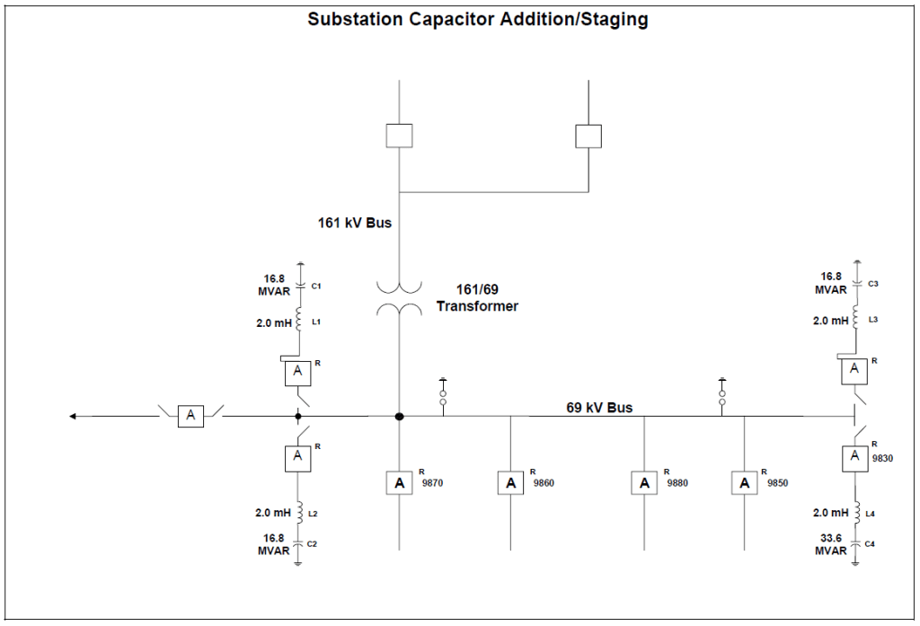
Abstract: A utility presently operates two 16.8 MVAr capacitor banks in a 161/69kV substation. Supplied by this substation are residential, commercial, and industrial loads, including a steel manufacturing facility. For increased voltage support, the utility is investigating the installation of three additional 16.8 MVAr, 69kV capacitors to be installed within the substation. Concerns have been raised with regards to the change in resonance as a result of these additional capacitors. The proposed capacitors could result in resonance conditions that could be excited by the locally operated arc furnace, thus possibly producing high levels of voltage distortion at the substation. This case study presents some of the findings associated with a resonance study that included power quality monitoring and harmonic distortion simulations.
INTRODUCTION
The scope of this study is to investigate the impact a capacitor bank has on the harmonic impedance at a utility owned, 69kV substation. The utility presently operates two 16.8 MVAr, 69kV capacitor banks at the substation. Upgrade plans include the installation of three additional 16.8 MVAr banks. For regulation of the 69kV bus voltage, automatic capacitor controls will provide staging of capacitors in 16.8 MVAr increments, from 0 to 84 MVAr. Due to a locally operated arc furnace, there are concerns that the additional capacitance could result in a shift in resonance; thus possibly resulting in overvoltage conditions due to excitation from the arc furnace. Of particular interest is the impact on harmonic distortion levels that result due to the interaction (resonance) between the capacitors and system impedance.
The scope of this harmonic evaluation study includes:
− Frequency Response Evaluation − Field Measurements − Harmonic Distortion Evaluation
SYSTEM MODEL DESCRIPTION AND DEVELOPMENT
A one-line diagram of the substation and surrounding transmission system is shown in Figure 1 and Figure 2.
Figure 1 – Oneline Diagram of Utility Substation
Figure 2 – Oneline Diagram of Surrounding 69/138/161kV Transmission System
The system model was developed using Electrotek’s SuperHarm® program. A three-phase model was used to simplify the analysis of transformer connections on harmonic cancellation. All transmission lines were modeled using a three-phase PI model, thus taking into consideration charging capacitance. Linear load was modeled to provide a realistic amount of system damping. Without these loads, the simulation results would be too conservative, especially at or near system resonance. Transformers were modeled using the SuperHarm three-phase transformer model. Transformer test report data was used when provided, and a default X/R ratio of 20 was used when resistances were not available. A typical capacitance of 16nF/mile was used to represent the charging MVAr of the overhead lines.
Analysis of Resonance Concerns for Harmonics
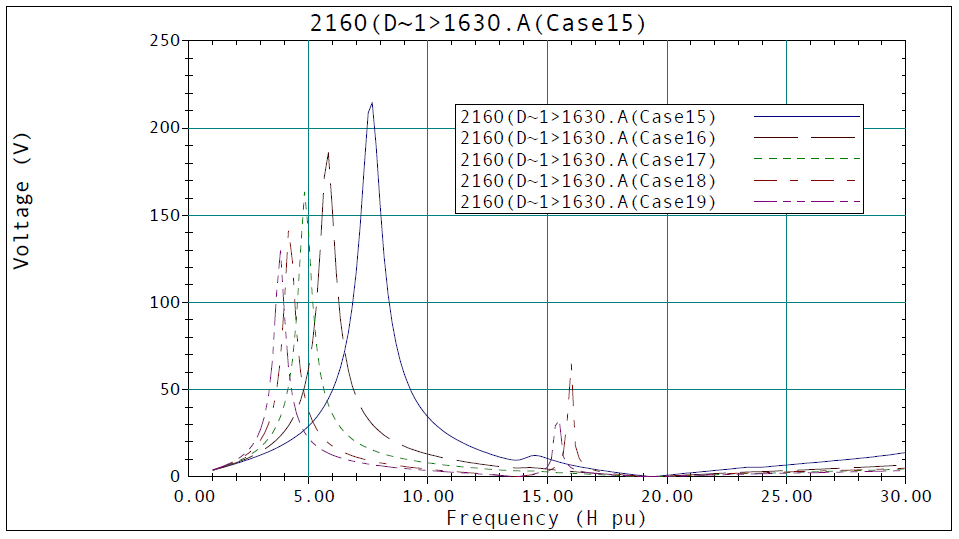
Frequency scans were performed at the substation to evaluate the affect of different capacitor configurations on system resonance. The scans demonstrate the expected harmonic voltage at the 69kV level per amp of harmonic current injected into the system. A summary of some of these cases is described in this section.
Figure 3 illustrates the affect of staging the substation capacitors (C7) from 16.8 MVAr to 84 MVAr on system resonance. For Case 15 (16.8 MVAr capacitor), a significant amount of resonance occurs between the 7th and 9th harmonic. As additional capacitance is added, this resonance is slightly decreased in magnitude. Unfortunately, this resonance is shifted to lower harmonic values (5th harmonic for Case 17 and 3rd harmonic for Case 19).
Figure 3 – Frequency Scan: Cases 15-19
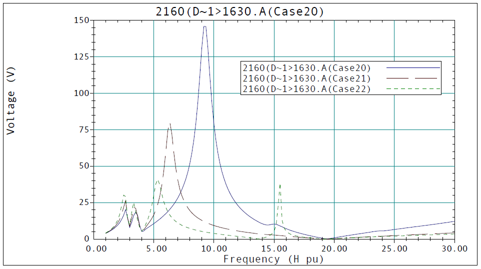
Figure 4 demonstrates the result of 3 levels of capacitance at the substation (C7 – 16.8, 50.4, and 84 MVAr) and capacitor banks C1, C2, C3, C4, and C5. Compared to Figure 3, the overall affect on resonance is a slightly decreased magnitude with a shift to higher harmonics.
Figure 4 – Frequency Scan: Cases 20-22
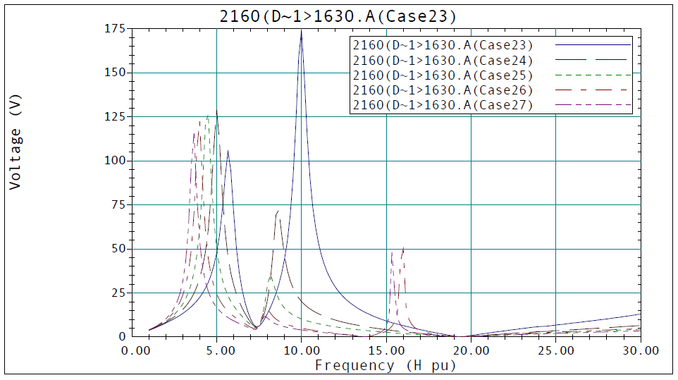
The cases shown in Figure 5 are similar to that of Figure 3 with the exception of the added 24.4 MVAr capacitor C6. As illustrated in Figure 5, the interaction of the substation capacitors and C6 have a strong impact on the overall system resonance at the substation. Increased resonance occurs at the 9th harmonic (Case 24) and 10th (Case 23). High levels of resonance also occur between the 3rd and 6th harmonics for all five cases.
Figure 5 – Frequency Scan: Cases 23-27
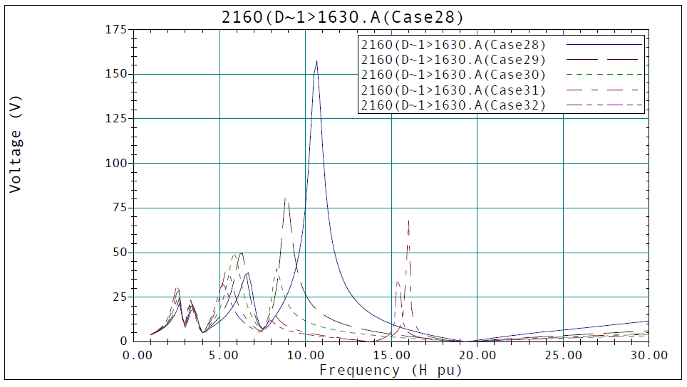
Figure 6 illustrates the affect of total capacitance (all capacitors switched in at the 13.2 kV level and C6) with the substation capacitors varied in 16.8 MVAr stages. The affect of additional capacitors at the 13.2 kV level have an overall positive effect on system resonance by reducing the magnitude of the lower order harmonic resonance considerably (compared to Figure 3 and Figure 5). High resonance conditions, however, do occur at the 11th harmonic (Case 28) and the 9th harmonic (Case 29).
Figure 6 – Frequency Scan: Cases 28-32
Field Measurements – Power Quality Monitoring
A Dranetz-BMI PQNode 8020 was installed at the substation and power quality data was collected for a period of 30 days. The PQNode monitored three-phase voltage (line-to-line) and current on the 69kV bus supplying the feeder to the arc furnace.
This section will summarize the data collected.
During the 30 day monitoring period, the arc furnace was not fully operational, thus limiting the amount of usable data for statistically characterizing the harmonic content on the feeder. During the first week of monitoring, arc furnace was not operating 100% of the time, and unfortunately, it was switched completely offline for approximately two weeks for routine maintenance, thus limiting the amount of usable data to roughly two weeks.
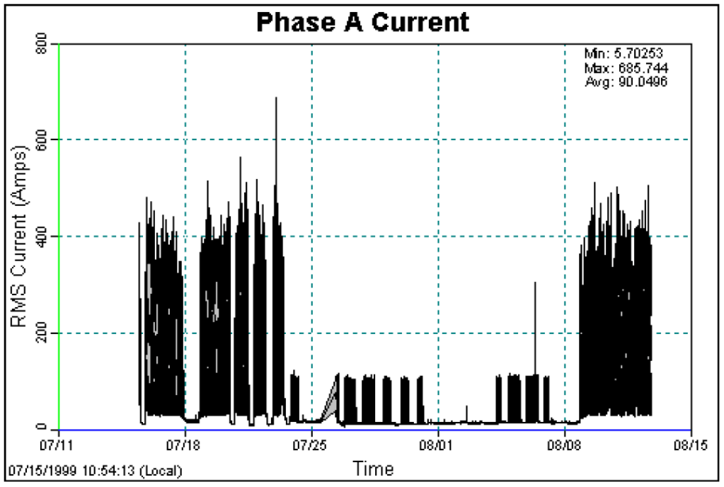
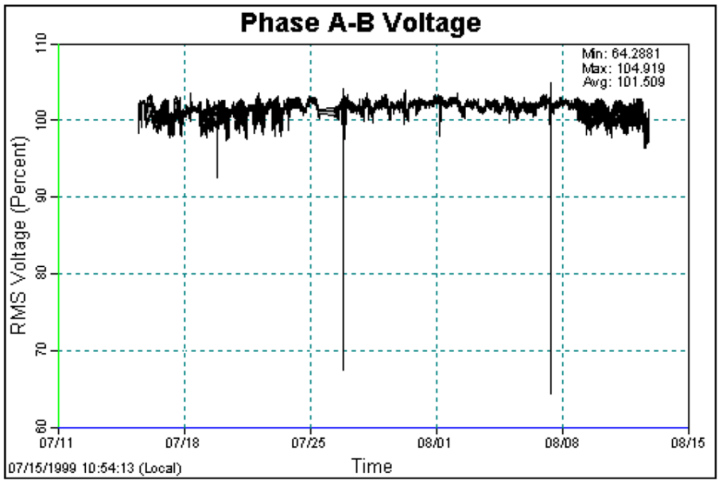
Figure 7 and Figure 8 illustrate the RMS line current and line-to-line voltage measured on the arc furnace feeder for the 30 day period. The various operating conditions in which the furnace undergoes are most evident in the current measurements.
Figure 7 – Measured A-Phase RMS Line Current (7/15 – 8/14)
Figure 8 – Measured VAB (7/15 – 8/14)
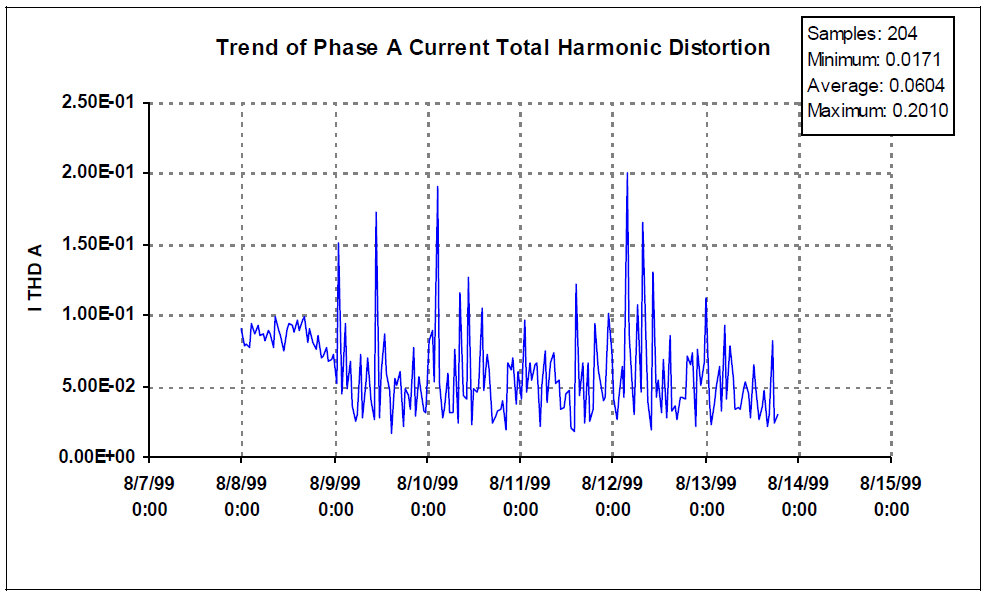
Figure 9 and Figure 10 illustrate the Phase A current THD from 8/8/99 to 8/14/99. Using the Electrotek/EPRI PQView® software, a statistical analysis of the measured data was easily performed with the results shown in Figure 10. These calculations were also performed for both B and C phases.
Figure 9 – Trend of Phase A Current THD
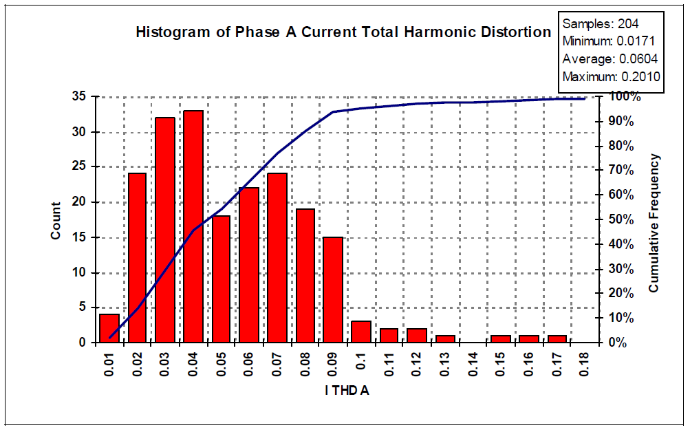
Figure 10 – Histogram of Phase A Current THD
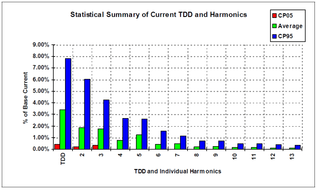
Using the data shown in Figure 10, PQView was used to calculate the average, CP05, and CP95 harmonic current values over this period. The statistical summary for the TDD and harmonics are shown in Figure 11.
Figure 11 – Average, CP05, and CP95 Harmonic Current Measured 8/8 – 8/14 Note: Base Current CP99 – 240A
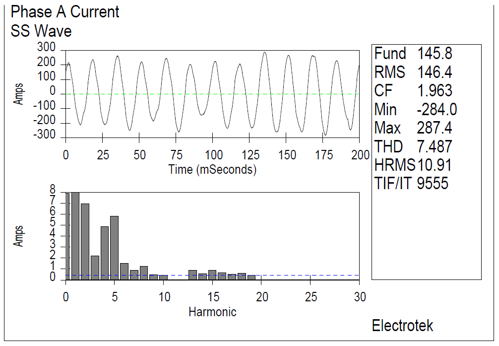
Using the data in Figure 11, a representative current spectrum, shown in Figure 12, was chosen from the 12-cycle samples taken. The fundamental (and corresponding current spectrum) was scaled up from 150A to 240A, a factor of 1.6, to simulate CP99 conditions. By doing so, this creates a considerably conservative approach. This scaled current spectrum was then used to represent the nonlinear characteristics of the arc furnace load.
Figure 12 – Snapshot of Current Spectrum for Distortion Simulations
Harmonic Distortion Simulations
Using the system model developed for the resonance simulations, the scaled harmonic spectrum in Figure 12 was modeled in SuperHarm as a non-linear load connected directly to the utility substation 69kV bus. A conservative approach was taken in modeling the transmission system by removing the parallel resistance used with each source equivalent. This parallel resistance provides the damping necessary to estimate “actual” system conditions. By removing this resistance, “worse than actual” system conditions can be simulated, thus providing extremely conservative results. Note: Because this source damping is not included, a direct comparison with measured THD values cannot be performed.
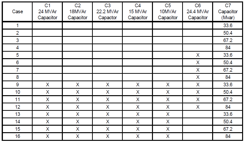
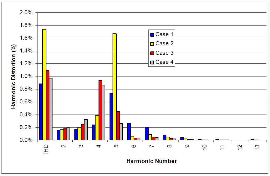
Based upon the frequency scan results found in Figure 3 through Figure 6, various worst case system configurations were considered for calculating the expected THD as the additional 50.4 MVAr capacitors are added at the utility substation. These cases are summarized in Table 1. For each of the below cases, the amount of capacitance at the substation is increased from the presently operating 33.6 MVAr to 84 MVAr in increments of 16.8 MVAr.
The capacitor configurations considered in Cases 1 through 8 are not considered realistic scenarios. However, to simulate the absolute worst case conditions, they were included.
Table 1 – Summary of Harmonic Distortion Simulations Performed
As seen in Figure 13, with only capacitors operational at the substation, the maximum THD value calculated is found in Case 2, with less than 1.8% THD.
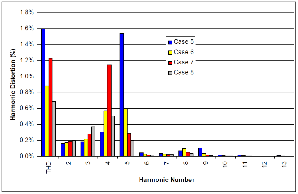
With the C6 24.4 MVAr capacitor online (Figure 14), the maximum THD values are found in Case 5, which represents the existing substation capacitor configuration. The maximum THD value reaches 1.6%, with the 5th harmonic topping at approximately 1.5%. As capacitance is increased at the substation, it is shown that the THD values are actually reduced in magnitude.
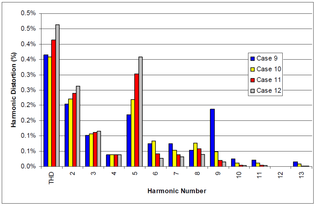
Figure 15 represents typical system capacitor configurations with the addition of C1, C2, C3, C4, C5, and C6 capacitors in service. The additional capacitance reduces the THD to approximately less than 0.5% for all cases. This reduction in THD is due to the reduced driving point impedance as the additional capacitors are switched into service (see Figure 5 and Figure 6).
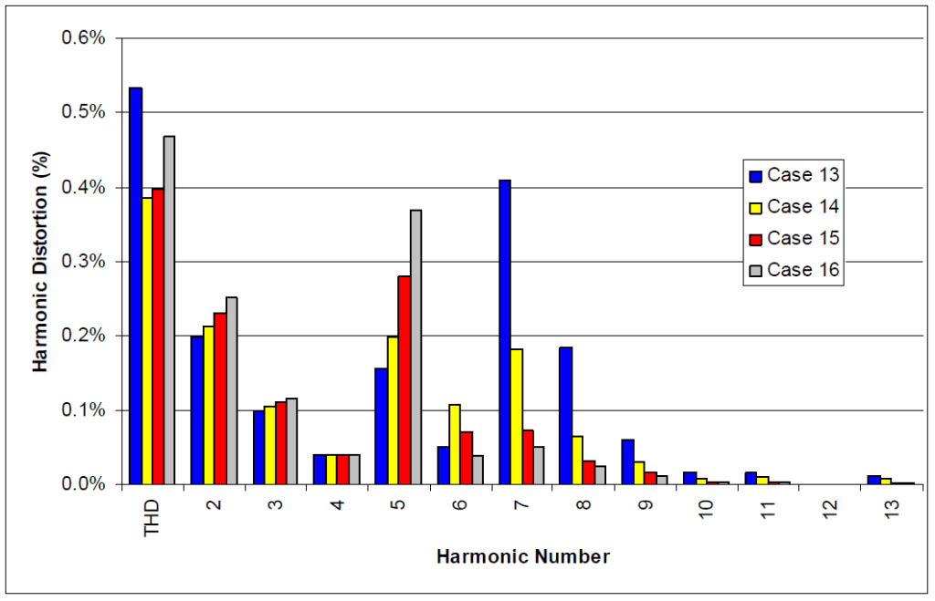
Similar results are found with the C6 24.4 MVAr capacitor taken out of the circuit (Figure 16). The maximum THD value reaches approximately 0.5%.
The purpose of this study was to investigate the possible resonance conditions that would occur with the introduction of 3 additional 16.8 MVAr capacitors at a utility-owned substation and to determine if any harmonic distortion limits would be exceeded due to excitation from a locally operated arc furnace. A complete three-phase model of the substation and surrounding transmission system was modeled in SuperHarm and the frequency response characteristics were examined for various system capacitor configurations.
A wide range of capacitor combinations was simulated using SuperHarm. As shown in Figure 3 through Figure 6, the introduction of the additional 3 capacitor banks at the substation reduces the magnitude of the present harmonic resonance. However, as a result of the added MVAr introduced into the system, the resonance frequency is also reduced to lower order harmonic values. This shifting of harmonic resonance has resulted in peaks occurring around the 3rd, 5th, and 7th harmonics.
With the locally connected arc furnace, it was quite possible for the furnace to excite this lower-order resonance, thus resulting in extreme overvoltages occurring at the substation. Due to the shifting of resonance to the 3rd, 5th, and 7th harmonics, it was determined that additional investigation would be required before conclusions with regards to possibly harmonic distortion problems could be made.
The second portion of this study involved monitoring the 69kV bus for possible harmonic currents that could excite the resonant conditions as a result of the additional capacitor bank installation. To simulate the affects of the arc furnace, the measured data was then incorporated into the three-phase model developed previously.
The harmonic distortion simulations proved that the amount of harmonic current being drawn by the arc furnace was not enough to cause problematic voltage distortion levels. The maximum voltage distortion levels were calculated at approximately 1.8%, well below the 5% THD limit specified in IEEE Std. 519-1992. Therefore, the additional three capacitor banks will not cause excessive voltage distortion at the utility substation and surrounding transmission system.
REFERENCES
1. IEEE Std. 519-1992, “IEEE Recommended Practices and Requirements for Harmonic Control in Electrical Power Systems.”
Published by Prithwish Mukhopadhyay, General Manager, prithwish.mukhopadhyay@posoco.in, Rajkumar Anumasula, Senior Engineer, rajkumar@posoco.in, Abhimanyu Gartia, Deputy General Manager, agartia@posoco.in, Chandan Kumar, Engineer, chandan.wrldc@posoco.in, Pushpa Seshadri, Chief Manager, pushpa_seshadri@posoco.in, Sunil Patil, Engineer, skpatil@posoco.in , WRLDC, Mumbai, India
Abstract — Synchrophasors are used extensively in Indian Grid to detect and analyze faults occurring in the system. This paper majorly discusses the case studies of power system faults that occurred in the Indian grid and its identification and classification using data obtained from Synchrophasors. The types of faults identified include symmetrical and unsymmetrical faults in power system. Further in case of single phase to ground faults, the successful, unsuccessful and non -operation of autoreclosure has been verified. Data from Phasor measurement units (PMUs) helped in identifying the fault recovery time and operation of autoreclosure and provided a strong tool for monitoring the status of the protection system in the grid. A comparative analysis of the disturbance recorder files and the synchrophasor data has also been discussed in this paper. The comparative analysis is used for validation of the DR and Synchrophasor data. This paper has led to the development of disturbance analysis tool for fault analysis using both DR and Synchrophasor data which will ease the system operator decision making ability while taking decision during a contingency in the system.
Index Terms—Synchrophasor, Faults, Autoreclosure, Indian grid, Disturbance recorder.
I. INTRODUCTION
Power system operation in India is complex due to disparity in geographical distribution of resources and loads, network complexity with rapid changes in network configuration and increasing combination of UHV, EHV, HVDC lines and FACTS devices in the system. Synchrophasor measurement units also known as “Phasor measurement units (PMUs) have become a very effective tool for system monitoring and analysis.
The Indian Grid is a large synchronous grid which constitutes of Eastern, Northern, North-Eastern, Southern and Western grids. Synchrophasor measurement units have been deployed in each regional grid under the pilot projects for monitoring and development of analytics which will help in system operation [1-2]. This has proved to be a boon for understanding the behavior of Indian power system. The high resolution data obtained from PMUs (25 samples/sec) with accurate time stamping provides a continuous snapshot of the system. Among the various applications explored from this technology, fault analysis is used extensively for understanding the sequence of events and also for strengthening protection schemes. It has helped in post facto analysis and real time detection of faults occurring in the grid.
In the Western regional grid, ,PMUs are placed strategically covering all types of buses like generator buses, intermediate pooling stations, load centers, HVDC substations etc. [2]. The potential transformer (PT) of the Bus and current transformer (CT) of the feeders have been used as analog inputs to the PMUs. Prior to Synchrophasor technology implementation in India, the identification, detection and classification of fault was confirmed from the Disturbance recorder (DR) files, Sequence of events (SOE) from the Relays and Sub-station SCADA. Obtaining these details from various substations resulted in delayed analysis and information about the power system phenomenon. With the PMU data available at control centers, the fault can be detected identified and classified in real time by observing the trends in various parameters of the system. This has saved a lot of time for analysis as the nature and type of fault can be confirmed at the control center itself although the DR and SOE are still used for its confirmation.
This paper is focused on the fault analysis of EHV transmission lines and bus bar, their characterization using synchrophasor and their validation using disturbance recorder data. Section II illustrates the single phase fault in the Indian power system followed by the Sections III and IV where phase to phase and three phase fault have been discussed. Section V discusses the validation of observations from Synchrophasor data with DR for power system. Section VI concludes the paper.
II. SINGLE PHASE TO GROUND FAULT
Single phase to ground fault is the most common type of fault in power system. Such faults are very common in transmission lines and can be either temporary/transient or permanent in nature. The ground path provided by trees, fogs etc. are temporary in nature and these ground paths gets cleared immediately. The permanent nature fault appears in case the conductor breaks down (in case of transmission line), current or potential transformer bushing burst (in sub-station) or by some other permanent grounding path. To avoid permanent isolation of an element in case of a transient fault, auto-reclosure (A/R) for single phase faults is provided for 400 kV and higher level EHV transmission lines On the basis of that, four cases of phase to ground fault are discussed here which are:
1. Single phase to earth fault on transmission line with successful A/R 2. Single phase to earth fault on transmission line with unsuccessful A/R 3. Single phase to earth fault on transmission line with no A/R. 4. Single phase to earth fault on Bus bar.
The first case of single phase to earth fault with successful auto-reclosure is shown in figure 1 and figure 2 where a fault on B phase to earth occurred on 400 kV Jabalpur-Vindhyachal circuit 4. It can be observed that when a single phase fault occur on transmission line the voltage of faulty phase dips to a lower value while remaining phases will observe a smaller dip due to unbalance in the system as the fault is being fed by the bus whose voltage has been as shown in figure 1.
Figure 1. Voltage of 400 kv Jabalpur bus from Synchrophasor data during single phase to ground fault on 400 kV Vindhyachal-Jabalpur circuit 4.
Figure 2. Current of Vindhyachal-Jabalpur circuit 4 observed from Jabalpur end from Synchrophasor data
Figure 2 shows how the fault current is increased in the faulty phase of the circuit indicating fault feeding from the affected phase. The line protection operated in zone 1 from both end and the faulty phase got isolated from both end resulting in recovery of voltage in faulty phase while current in the phase became zero. This has resulted in A/R initiation for the faulty phase and after 1 second, that phase got reclosed and further no fault was sensed resulting in successful auto reclosure. The line came back in service and the system again came to a balanced state. The voltage channel in PMU is obtained from the Bus PT so it will not become zero but due to the fault, the voltage of bus will get unbalanced and will observe a large dip in faulty phase.
Second case is the single phase fault with unsuccessful auto re-closure of the line. In cases where the fault is not of transient nature, permanent tripping of the line is required. One such case was observed in 400 kV Solapur Parli circuit 1. Figure 3 shows the voltage of 400 kV Solapur Bus during the fault while figure 4 gives the current observed in the faulty circuit from Solapur end.
Figure 3. Voltage of 400 kV Solapur bus during single phase to ground fault on 400 kV Solapur Parli 1 circuitfrom Synchrophasor data
Figure 4. Current of 400 kV Solapur parli citcuit 1 observed from Solapur end from Synchrophasor data
B phase to earth fault occurred in the 400 kV Solapur Parli circuit 1 due to the heavy rainfall in the area. As observed from the voltage of 400 kV Solapur in figure 3, the voltage of faulty phase dipped to a very low value due to feeding of the fault through the bus. The fault current as shown in figure 4 increased and with carrier aided zone 1 protection, the line tripped in the faulty phase from both ends. A/R was initiated after one second. The faulty phase of the circuit got reclosed but due to permanent nature of fault, all the three phases tripped thus isolating the faulty line.
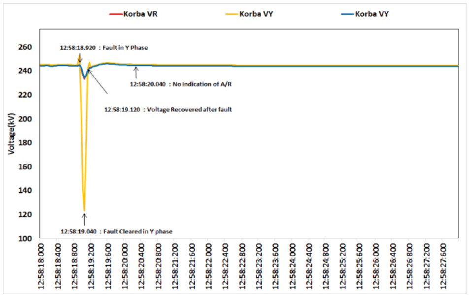
There are cases in which the Auto-reclosure did not occur on the line in case of single phase to ground fault. This is mainly due to issue with the carrier communication or relay. Such cases are very much essential to be analyzed and informed to the concerned utility to rectify it at the earliest. One such case has been shown in figure 5 and 6 where the auto reclosure activity was not observed during single phase to earth fault on 400 kV Korba-Bhatapara.
Figure 5. Voltage of 400 kV Korba bus during single phase to ground fault on 400 kV Korba Bhatapar circuit from Synchrophasor data
On 400 kV Korba Bhatapra circuit, Y phase to earth fault occurred on the circuit. As observed from the figure 5 , the faulty phase voltage dipped at Korba and the fault got cleared with operation of line protection [2]. While figure 6 shows the current of the feeder from Korba end which confirms that the all the three phases of the line tripped rather than single phase with A/R initiation. This was informed to the concern utility and rectified.
Figure 6. Current of 400 kV Korba Bhatapara citcuit observed from Korba end from Synchrophasor data
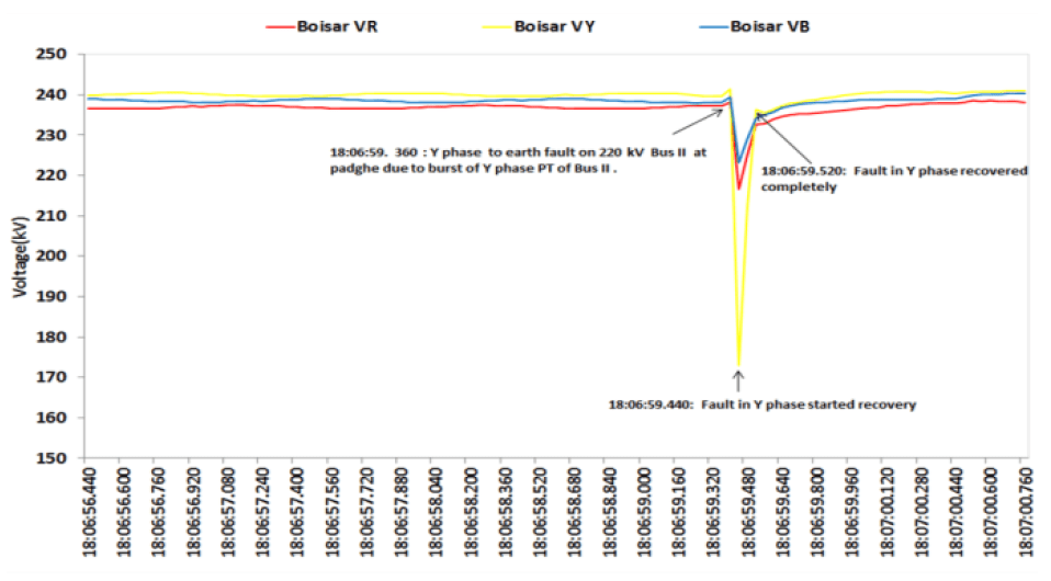
The last case in the section of single phase to ground fault is associated with bus fault, which in general occur due to problem with CT/PT bursting. One such case of bus fault at 220 kV level was observed by the synchrophasor unit installed at 400 kV nearby Bus is shown in figure 7.
Figure 7. Voltage of 400 kV Boisar bus during single phase to ground fault on 220 kv Padghe Bus II from Synchrophasor data
From Figure 7, it can be observed that Y phase to ground fault occurred at Padghe Sub-station on 220 kV Bus II due to bursting of Y phase Bus PT. This resulted in fault feeding by the nearby buses resulting in voltage dip as observed in figure 7. The fault got cleared in 160 ms with the operation of 220 kV Bus bar protection of Bus II.
With this it can be understood that how easily single phase fault can be analyzed at control centre without any DR/EL from the sub-station with the help of synchrophasor data.
III. PHASE TO PHASE FAULT
The second category of fault in the power system is phase to phase fault. In such cases, the fault may involve a ground path or may not. Such types of faults are rare in nature and generally found in transmission lines.
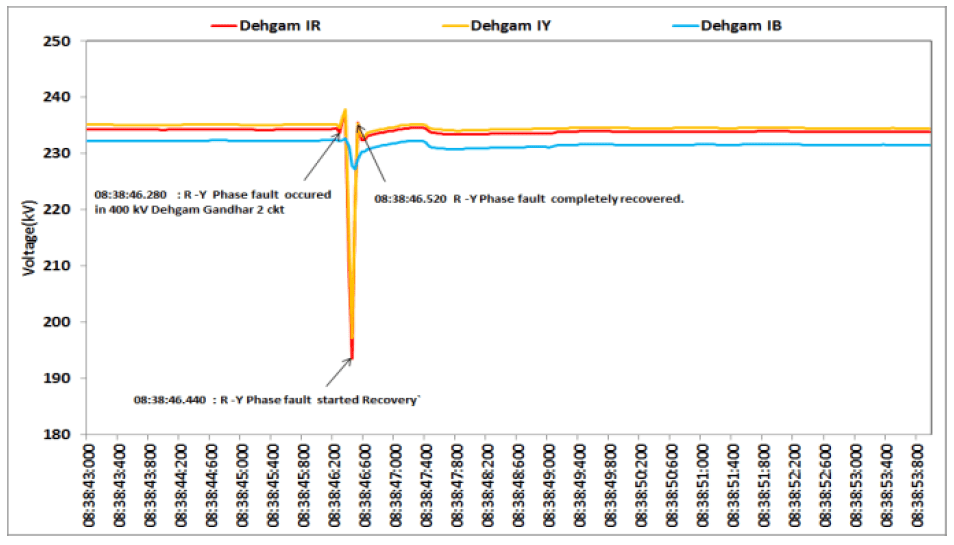
The case as shown in figure 8 and 9 is for the R-Y Phase fault on 400 kV Dehgam-Gandhar circuit 2. It can be observed from figure 8 that the phase voltages of the faulty phases have dipped to a lower value till the fault got cleared with the tripping of line. The current observed from Dehgam for this line show that the fault current in the faulty phases has increased drastically and it got cleared with tripping of the line from both end on zone 2 protection.
Figure 8. Voltage of 400 kV Dehgam bus during Phase to Phase fault on 400 kV Dehgam-Gandhar circuit 2 from Synchrophasor data
Figure 9. Current of 400 kV Dehgam- Gandhar citcuit 2 observed from Dehgam end from Synchrophasor data
It can be observed that how easily the phase to phase fault can be detected with the synchrophasor data. This has reduced the time taken for analysis of any complex fault in power system.
IV. THREE PHASE FAULT
One of the most severe and rare occurring fault in the power system is three phase fault. This fault may or may not involve ground. The severity is very high and may result in commutation failure of nearby HVDC and stalling of AC motor in the nearby area.
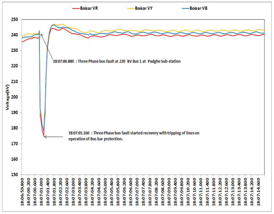
Two cases are considered here for example, one at a bus and other on the transmission line. Figure 10 shows the voltage of nearby bus during a three phase fault on 220 kV Bus 1 at Padghe. Voltage has dipped in all the three phases as the fault was being fed by the nearby buses. Figure 11 shows the current in the transmission line connecting the two sub-stations, which has increased as the Boisar Bus is feeding the fault at padghe. The fault got cleared after the operation of bus bar protection.
Figure 10. Voltage of 400 kV Boisar bus during three phase fault on 220 kV Dehgam-Gandhar circuit 2 from Synchrophasor data.
Figure 11. Current of 400 kV Boisar-Padghe citcuit duing the three phase bus fault on 220 kV Padghe Bus 1 from Synchrophasor data
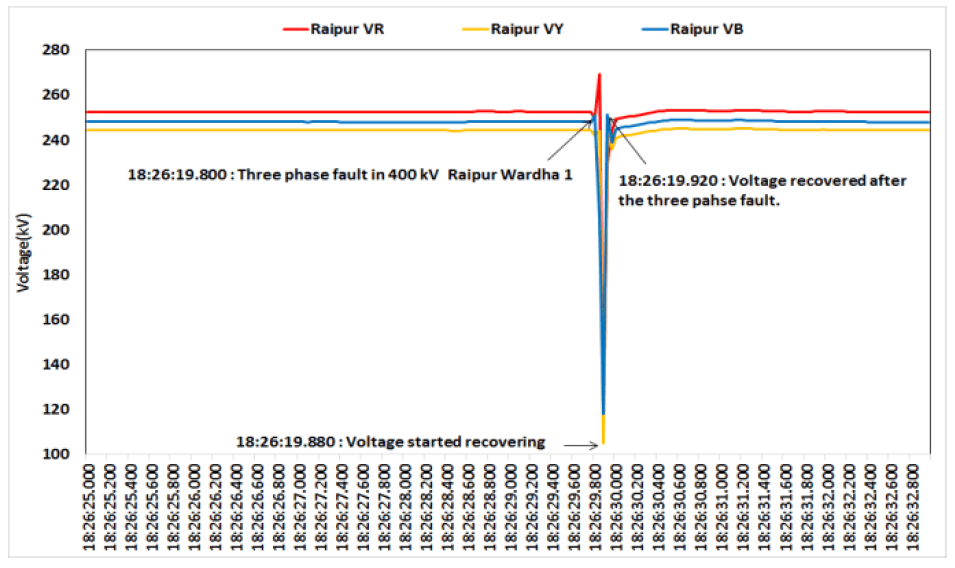
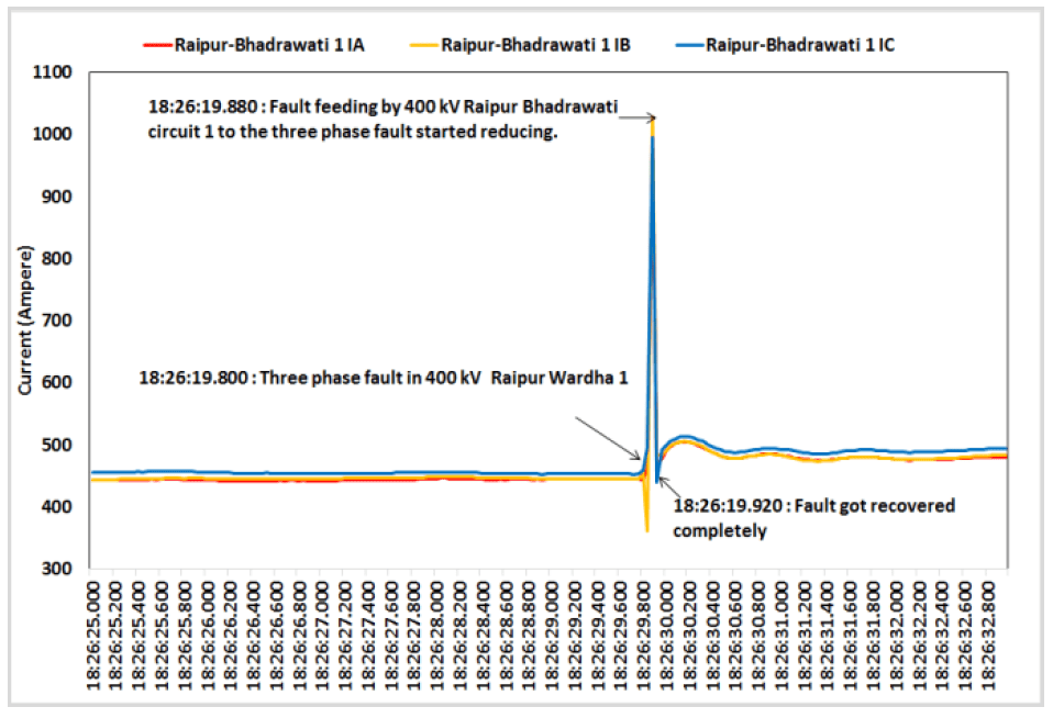
The second case is of the three phase fault on a transmission line. Figure12 and 13 shows the synchorphasor data for the three phase fault on 400 kV Raipur Wardha circuit 1. From figure 13 it can be seen that during three phase fault on 400 kV Raipur wardha 1 circuit , the voltage of the Raipur bus I all the three phases dipped to a lower value and recoverd with tripping of circuit on zone 1 line protection.
Figure 12. Voltage of 400 kV Raipur bus during three phase fault on 400 kv Raipur –Wardha circuit 1 from Synchrophasor data.
Figure 13. Current of 400 kV Raipur Bhadrawati circuit 1 observed from Raipur end from Synchrophasor data
With this all the three types of fault has been discussed with the help of synchrophasor data. This has shown the importance of synchrophasor measurement units in fault analysis and event detection at control centers. In the next section the validation of synchrophasor data with the disturbance recorder file is discussed for determining up to what extent it can be used and what are their limitations.
V. VALIDATION OF SYNCHROPHASOR DATA FOR FAULT ANALYSIS AND ITS LIMITATION
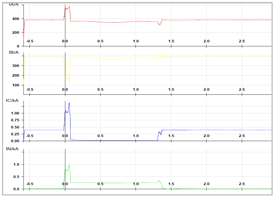
Synchrophasor data has come out as a very effective tool for analyzing faults in power system in real time. But the synchorphasor data has its own limitation compared to the disturbance recorder file which has higher sampling rate (kHz). Figure 14, 15, 16 shows the DR for the first three events discussed in section II in case of single phase to earth fault with successful A/R, unsuccessful A/R and no A/R respectively using SIGRA [3]. The synchorphasor are the fundamental frequency component calculated using Discrete Fourier Transform (DFT). So higher harmonic are being neglected which may result in different fault current observed from synchrophasor data and actual data from fault recorder.
Figure 14. Current from the DR of 400 kV Jabalpur -Vindhyachal circuit 4 from Jabalpur end for the single phase fault (successful A/R).
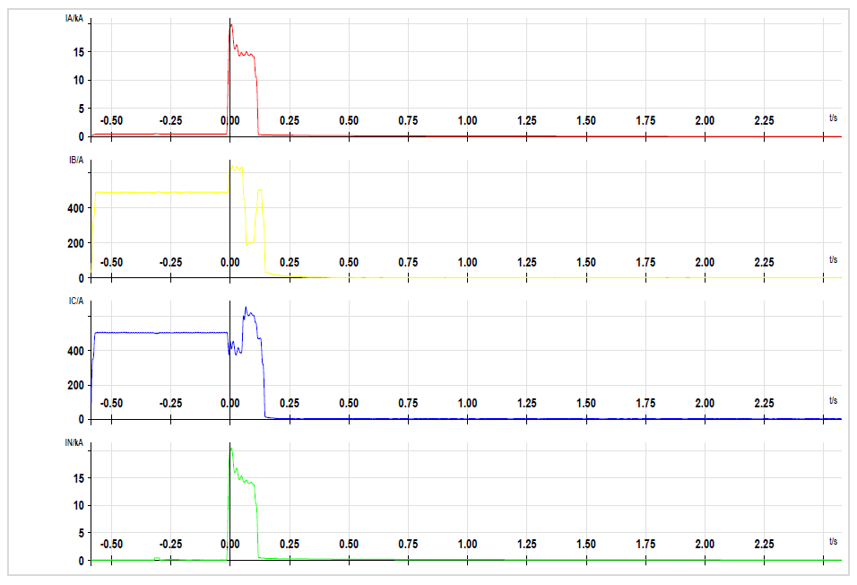
Figure 15. Current from the DR of 400 kV Solapur -Parli circuit 1 from Solapur end for the single phase fault (unsuccessful A/R).
Figure 16. Current from the DR of 400 kV Korba Bhatapara circuit 1 from Korba end for the single phase fault (No A/R)
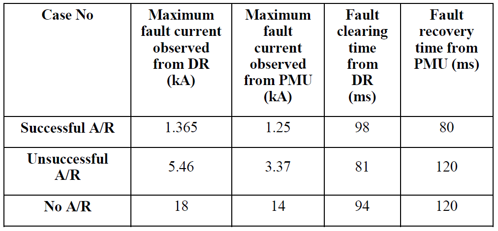
The validation analysis of the three cases is shown in table 1. Here major two parameters i.e. fault current value and fault clearing time has been tabulated for all the three cases.
Table I. Validation of DR and Synchrophasor Measurement During Fault
.
It can be observed that fault clearing time from DR and PMU has slight difference which is attributed to mainly three factors:
1. Reporting rate of PMU (here at every 40 ms) 2. DFT Window length (generally varies from two cycles to 10 cycles). 3. Time stamping of phasor (time stamping at the starting/middle/end of DFT calculation window) [4].
This in general result in a ±40 ms error in the time for fault recovery time [2]. This can be improved with increasing the reporting rate of the PMU.
Also, when the fault current is analyzed it can be observed that there is a difference between the maximum fault current from synchrophasor measurement and disturbance recorder, both of which are taken from the same CT of the feeder. This can be due to various reasons and out of these major two are:
1. PMU uses measurement core while the DR uses the protection core of the CT which is having higher accuracy. (Although PMU can be made to use protection core of the CT also, but in India measurement core of the CT is used)
2. The second reason is the contribution of higher harmonics during faults.
During faults, the fault current is having DC, Fundamental frequency component and higher harmonic component. DR measured currents are having all these components. While synchrophasor is giving only the fundamental frequency component resulting in lower current values. Figure 17 shows the various components in the faulty phase current for the three cases discussed for validation in this section. It can be observed that the Current associated with fundamental component of the frequency are very close to what being observed by the synchrophasor units.
Figure 17. Various compoent of Current when maxium fault current appear in the three cases 1. Successfulr A/R 2. Unsuccesdful A/R and 3. No A/R.
Thus, it can be inferred that, synchrophasor data has given a very good insight into the various aspect of fault observed in the power system. Synchrophasor data can be used for event detection engine at control centers in real time by setting various thresholds to detect the individual types of faults. It also helps in quicker detection of A/R in case it has been enabled during single/three phase fault in zone 1 for transmission line. The extent of fault current signifies the severity of fault to the real time operator in taking decision for charging of the faulty line. Synchrophasor data in combination with field records will make fault analysis easier.
VI. CONCLUSION
This paper has discussed the various types of faults as observed from the synchrophasor measurements. This has helped in finding the various characteristic of different types of faults in power system. The paper has led the basis of disturbance analysis tool development for analysis of the fault in offline mode with the helped of Synchphasor and DR data. Also has set path to the course of event detection engine in real time using synchrophasor data stream. Such development will help real time system operator to access the severity of power system faults and take corrective action to reduce its after effects.
ACKNOWLEDGMENT: The authors acknowledge the guidance and support given by managements of POSOCO as well as PGCIL and for permitting the publication of this paper. The authors are sincerely thankful to Shri. P.Pentayya, Ex General Manager, WRLDC for his guidance during Synchrophasor Pilot project implementation in western region. The authors are also thankful to WRLDC personnel for their support. The views expressed in this paper are of authors and not necessarily that of the organizations they represent.
REFERENCES
[1] “Synchrophasors Initiative in India,” POSOCO, New Delhi, Tech.Rep. July 2012 [2] “Synchrophasors Initiative in India,” POSOCO, New Delhi, Tech.Rep. December 2013 [3] “User Manual –Fault Record Analysis SIGRA 4 ”, Siemens [4] IEEE Standard for Synchrophasor Measurements for Power Systems, IEEE Std C37.118.1TM-2011,Dec.2011
Published by Lorenzo Mari, EE Power – Technical Articles: AC Equipment Grounding: Creating a Safe Fault Current Path to Ground, August 07, 2020.
Learn about the merits of the equipment grounding to protect people in faulted AC power systems.
Electrical equipment casings should be at earth potential under normal conditions. When a fault occurs in an ungrounded casing, it will remain energized, creating a threat to people’s safety. If you are grounded and touch that housing, a dangerous current will flow through your body.
The magnitude of this current may not be enough to activate the circuit protection, but it could be enough to kill someone. Equipment grounding provides a secure, low impedance path to ground, allowing a sufficient amount of current to flow to trip a breaker or blow a fuse, removing the hazard.
In the last article regarding AC equipment grounding, we analyzed the dangers of electric shocks. This article will focus on proper safety measures as noted by the National Electrical Code (NEC).
Equipment Grounding Regulations and Language
The basis of this article is the National Electrical Code (The NEC). The NEC is a set of rules and regulations for the safe installation of electrical equipment and wiring used in the United States and other countries. The methods discussed in this article are mainly for low voltage power, heat, and light.
One of the reasons for the misunderstandings that appear when handling the subject of equipment grounding is the use of inappropriate terms. To avoid this situation, everyone should speak the same language, and the recommendation is to use the terms defined in the NEC, Articles 100 – Definitions – and 250 – Grounding.
The use of unofficial or ambiguous terminology can cause confusion and increases the chance of making mistakes in grounding installations.
Three essential terms to be aware of are “grounded conductor,” “equipment grounding conductor,” and “grounding electrode conductor.”
The NEC is a complex set of standards. This article will give a general overview. Readers should still consult the NEC before working with AC equipment grounding techniques.
Equipment Grounding Basics
The term equipment grounding refers to the grounding of parts of the electric system that do not regularly conduct electricity, like service equipment, the frames of appliances, metal conduits, and metal shields of shielded cable. The primary purpose of equipment grounding is safety.
Grounding keeps all equipment at the same potential, decreasing the possibility of harming a person in contact with two metal parts that could have different potentials when electrical failures occur. This permanent joining of metallic parts to form an electrically conductive path is known as bonding.
When the electrical systems fail, people’s lives may depend on a proper grounding installation. Equipment grounding provides a dependable, low impedance path to the fault current for the correct operation of protective devices.
Equipment grounding and system grounding come together only at the power source, such as the service equipment.
Basic Concepts of Grounding for Safety
The NEC defines service as the conductors and equipment for delivering electric energy from the serving utility to the wiring system of the premises served. But the conductors and equipment are feeders, and not a service, when other than the serving utility supplies the electric energy.
In this article, we’ll use the terms service, service equipment, and service entrance. The service equipment may comprise one or more main fused switches or circuit breakers.
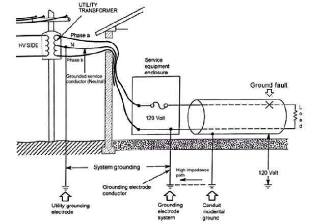
Figure 1 shows a 3-wire, single-phase overhead service to a building. It starts at the service point on the load side of the transformer. The transformer usually belongs to the utility company, but may also be a customer’s property.
A load is any piece of equipment connected to the wiring that consumes power, like a lamp, a motor, a fridge, or a microwave oven.
The power comes into the premises over three conductors, the service-entrance conductors. The conductors marked a and b are ungrounded and called phase conductors or hot wires.
The conductor marked N, is the neutral or grounded conductor, grounded at the service equipment and the transformer. The voltage between a or b and the neutral N is 120 V; the voltage between a and b is 240 V.
A person touching a and b will receive a 240 V shock. Touching a or b and N will cause a 120 V shock. Note that N is grounded, and the person will also receive a 120 V shock by touching a or b while standing on the ground.
The utility company grounds the neutral at the transformer for three reasons:
• Connect the neutral to 0 V, ensuring that VaN = VbN = 120 V • Protect the load side from high voltages resulting from a primary-to-secondary short, a higher voltage line falling on the service-entrance conductors or a nearby lightning strike • Make sure that the neutral is grounded even if the connection at the service equipment is missing
Figure 1 also shows phase a supplying a single-phase, 2-wire, 120 V load. Here, conductor N is not a neutral but just a grounded conductor. The reason is that a neutral carries the unbalanced current of phases a and b, and in this circuit, the conductor takes all phase a (or load) current.
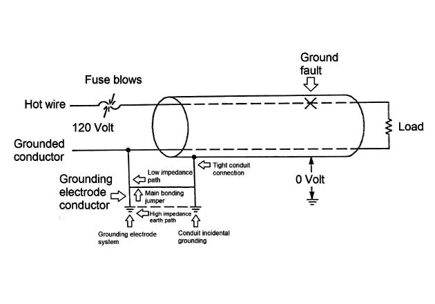
The conduit connection to the ground is accidental or incidental, meaning that the grounding is not by design. Incidental grounding happens when attaching the conduit to a support connected to the earth. So there is very high resistance in the ground circuit between the conduit and the neutral ground connection.
If the phase conductor insulation fails (ground fault), the fault current will flow through a high resistance circuit. It will not be of the magnitude necessary to operate the circuit protection. Then the conduit will be energized at 120 V, which will pose a risky condition for people who can touch it.
The conduit shown in Figure 1 represents any ungrounded metallic frame of electrical equipment.
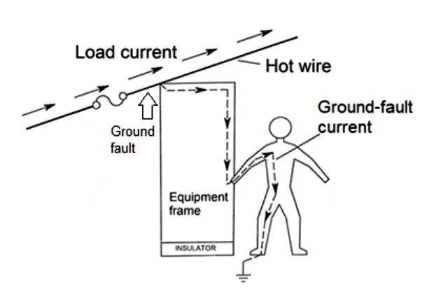
Figure 2 shows an ungrounded equipment frame under ground fault conditions. The protection devices do not clear the fault, allowing the structure to sustain 120V to ground. A person’s body in contact with a grounded element touches the frame and becomes part of the fault circuit. The dotted line shows the path the fault current follows through the body, a condition that will probably cause a sharp shock and perhaps death.
Figure 2. Shock hazard from an ungrounded equipment frame.
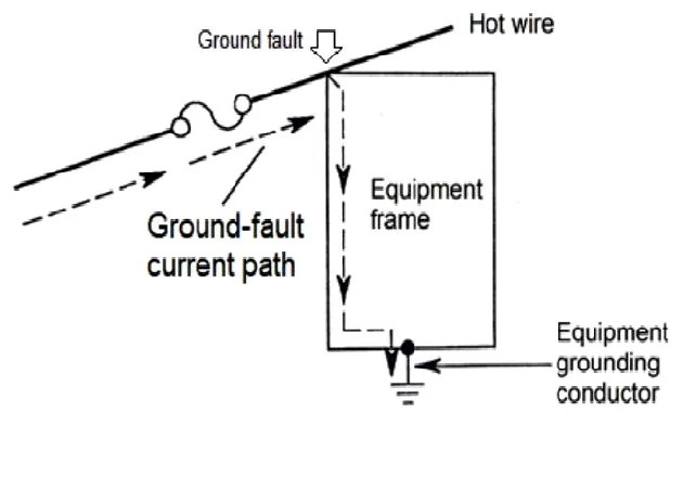
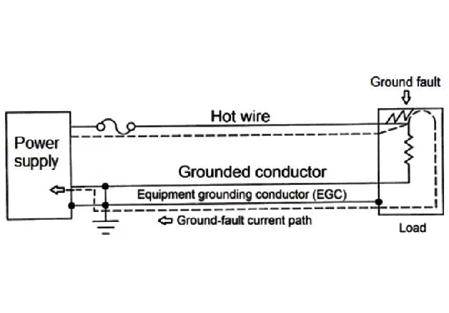
Figure 3 shows the same ground fault but this time with a grounded equipment frame. Here, a ground-fault current of sufficient magnitude flows to operate the circuit protection adequately, and the structure, at ground potential, does not pose a shock risk.
Figure 3. Ground-fault current path with the equipment frame grounded
Do not connect the equipment frame only to the physical ground, but in the way indicated by Article 250 of the NEC as described in the following paragraphs. The NEC prohibits using the earth as an effective fault-current path.
The Grounded Conductor
A grounded conductor is a system or circuit conductor grounded intentionally. A fundamental requirement to bear in mind is that a grounded conductor is never interrupted by a circuit breaker, switch, fuse, or another device unless this device opens the grounded and ungrounded conductors simultaneously.
The grounded conductor runs from the source to the load without switches or overcurrent protection, although it may be spliced or connected to terminals.
Once again, the grounded conductor, whether it is a neutral or not, is grounded twice. Once to the grounding electrode system at the service equipment, and once to the transformer serving the property.
No harm follows if someone touches an exposed grounded conductor or a component of the grounding electrode system, as described in the following paragraphs. Every time you touch a faucet or a water pipe, you are in contact with the grounded conductor.
The Equipment Grounding Conductor
Figure 4 shows a protective grounding conductor connected from the equipment frame to the system grounded conductor. This conductor is NEC’s equipment grounding conductor (EGC). It connects non–current-carrying metal parts of equipment together and to the system grounded conductor or the grounding electrode conductor, or both.
Figure 4. Ground-fault current path through EGC
The EGC does not carry current during regular operation, but it does when there are damages or defects in the wiring system or the connected pieces of equipment. The dotted line shows the path of the fault current. Since this path has a low resistance, the fault current will have the required magnitude to operate the protective devices.
The NEC recognizes that the EGC also performs bonding.
When using metal conduit or cable with a metal shield, the conduit or shield serves as the equipment grounding conductor. Figure 5 shows a metallic conduit fulfilling this task.
Figure 5. Metallic conduit as EGC
Although the metallic conduit provides an electrical path, loose connections could interrupt this grounding conductor. The recommended practice is to run an additional wire in each conduit to offer a continuous and reliable second route. By doing this, the fault current divides between the conduit and the additional wire.
Adding a wire does not decrease the need for electrical continuity between the housings and the conduits. Either way, the current will flow through the metal components and, if there are loose connections with high resistance, arcs and heating can occur with the risk of fire.
Figure 6 shows the EGC connections, in a 3-wire, single-phase service. The EGC goes from the equipment frame to the grounding terminal bar in the service equipment, bonded to its enclosure.
Figure 6. EGC connections, in a 3-wire, single-phase service
The Main Bonding Jumper
A bonding jumper connects two or more portions of the equipment grounding conductor throughout the electrical system, to ensure a ground-fault current path. But, the main bonding jumper, one of the most critical elements in the grounding system, connects the equipment grounding conductor, the service grounded conductor, and the grounding electrode conductor at the service, closing the fault circuit. It carries all the fault current from the equipment grounding arrangement returning to the source.
The Grounding Electrode System
The grounding electrode system is the physical connection to the earth. It bonds together the multiple electrodes that the building may have; using multiple grounding electrodes is more effective than depending on a single grounding electrode.
The electrodes permitted by the NEC for grounding are metal underground water pipe, metal in-ground support structures, concrete-encased electrodes, ground rings, rod and pipe electrodes, and plate electrodes.
The Grounding Electrode Conductor
The grounding electrode conductor connects the grounded conductor, the equipment grounding conductor, or both, to a point on the grounding electrode system or a single grounding electrode.
Figures 4, 5, and 6 show the relative location of the main bonding jumper, grounding electrode system, and grounding electrode conductor.
Effects of Several Grounding Connections
Except in some special applications, the equipment grounding conductor may be grounded at several points. But the neutral or grounded conductor must be grounded only at the service.
You may ask, why insulate the grounded conductor if it is grounded and there is no risk in touching it? The grounded conductor carries current, and without the insulation, it will contact the piping and other metallic structures.
The load current, supplied by the hot wire, will return to the source through the grounded conductor and all the grounding system, including the equipment grounding conductors, building steel, metal raceways, and water pipes.
These circulating currents will energize metallic frames and generate potential differences between the neutral of electronic equipment and ground.
The term used by the NEC is objectionable current. The NEC requires installing and arranging the grounding system in such a way that it will prevent objectionable current.
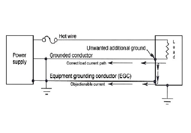
Figure 7 shows the flow of objectionable current when the grounded conductor has various grounding connections.
Figure 7. Objectionable current flowing through the equipment grounding conductor
If you suffer a shock when touching the fridge or a metal frame at home, the most likely cause is a neutral or grounded conductor connected to ground in more than one location. If you are wet, the shock can be much larger than expected.
Identification for Grounded and Equipment Grounding Conductors
The identification of grounded and equipment grounding conductors is critical, and the NEC gives methodical rules to accomplish this.
When using color codes, the general guidelines are:
Grounded conductors – A continuous white or grey outer finish or three continuous white or grey stripes along the conductor’s entire length on other than green insulation.
Equipment grounding conductors – For individually covered or insulated equipment grounding conductors, a continuous green outer finish, or green with one or more yellow stripes. The hot and grounded wires cannot use these colors. The EGC can also be bare.
There are no explicit color rules for hot wires. They may be any color excluding those mentioned above. Common choices are black, red, and blue.
Wiring Low Voltage AC Grounding Receptacles
It is essential to wire the grounding receptacles correctly to protect the users from shocks. There is no rationale for doing it wrong because this is an easy job.
Figure 8 shows the correct wiring of a conventional grounded receptacle. The installation follows the rule black to brass, white to light, green to green.
Figure 8. Correct wiring of a grounding receptacle
Although not mandatory, the typical installation practice is placing the opening for the grounding prong of the plug at the top. In this way, if a plug is inserted partially in the receptacle, exposing part of the prongs, and a metal object falls into the space between plug and receptacle, the grounding prong will block the object’s route to the hot prong, avoiding a ground fault.
Ground Fault Circuit Interrupter (GFCI)
Sometimes a standard circuit breaker or fuse cannot protect people against ground faults because the fault current is too low for them to operate. However, it could flow through a person in contact with the faulty equipment and a grounded surface.
A GFCI is an electronic device that effectively protects people by quickly interrupting the current to a circuit or a portion of it under ground-fault conditions. It is very sensitive and reacts to small fault currents, but there is no protection for phase-to-neutral and phase-to-phase faults.
The GFCI monitors the current to and from the load. If the wiring, a tool, or appliance allows some current to leak to ground, the GFCI will detect the difference in current in the two wires. When the fault current exceeds the trip level, it will disconnect the circuit in as little as 1/40 s.
The GFCI is an excellent supplementary safety precaution, especially when using electrical equipment in wet places like outdoors, bathrooms, and kitchens. The NEC requires the use of GFCI in specific locations in a dwelling and other units where the likelihood and severity of shocks are high. The GFCI will not prevent a person from receiving a shock, but it will open a circuit quickly enough to prevent injuries.
Several types of GFCIs are available, and they do not require an equipment grounding conductor.
A Review of Safe Grounding Techniques
The National Electrical Code (The NEC) establishes the minimum standards for wiring design and installation practice in the United States and other countries. These rules protect people from fire and other hazards.
In addition to the safety rules, the NEC provides technical terminology that, when used by everyone, reduces the misunderstandings that exist regarding the topic of grounding.
Equipment grounding connects to ground the metallic components of the electric system that do not carry electricity under normal conditions.
The grounded conductor connects to ground at the service only. It goes from the source to the load without any interruption or overcurrent protection.
The equipment grounding conductor, bonded to the grounded conductor, provides a safe and secure low impedance path for the ground-fault current, expediting the operation of overcurrent devices. It can be connected to the ground in several places.
The main bonding jumper is a crucial element that carries all the fault current from the equipment grounding arrangement back to the power supply.
The grounding electrode system provides the connection of the electrical system to the earth.
The grounding electrode conductor is the only connection to the grounding electrode system.
The NEC does not allow the flow of current through the grounding system – called objectionable currents – other than temporary ones that appear under ground-fault conditions.
The color of the insulation identifies the category of the conductor.
The use of a GFCI is convenient and required by the NEC in places with an increased chance of shocks, like wet environments.
For more information about AC electrical grounding, read other EE Power articles from Lorenzo Mari.
Author: Lorenzo Mari holds a Master of Science degree in Electric Power Engineering from Rensselaer Polytechnic Institute (RPI). He has been a university professor since 1982, teaching topics as electric circuit analysis, electric machinery, power system analysis, and power system grounding. As such, he has written many articles to be used by students as learning tools. He also created five courses to be taught to electrical engineers in career development programs, i.e., Electrical Installations in Hazardous Locations, National Electrical Code, Electric Machinery, Power and Electronic Grounding Systems and Electric Power Substations Design. As a professional engineer, Mari has written dozens of technical specifications and other documents regarding electrical equipment and installations for major oil, gas and petrochemical capital projects. He has been EPCC Project Manager for some large oil, gas & petrochemical capital projects where he wrote many managerial documents commonly used in this kind of works.
Published by Jacek DĄBROWSKI, Ewa KRAC, Krzysztof GÓRECKI Katedra Elektroniki Morskiej, Akademia Morska w Gdyni
Abstract. In the paper the results of long-time investigations of the photovoltaic installation situated in Gdynia Maritime University are presented. A short description of the considered installation and the weather station making possible continuous monitoring of weather parameters are included. The selected results of measurements of exploitive parameters of the considered installation obtained in the selected days and the corresponding to them results of measurements of power density of solar radiation are shown.
Streszczenie. W pracy przedstawiono wyniki długookresowych badań instalacji fotowoltaicznej zlokalizowanej w Akademii Morskiej w Gdyni. Zaprezentowano krótki opis rozważanej instalacji fotowoltaicznej i stacji pogodowej umożliwiającej ciągłe monitorowanie stanu pogody w miejscu zamontowania instalacji fotowoltaicznej. Pokazano wybrane wyniki pomiarów parametrów eksploatacyjnych rozważanej instalacji uzyskane w wybranych dniach oraz odpowiadające im wyniki pomiarów gęstości mocy promieniowania słonecznego. (Analiza długookresowej wydajności instalacji fotowoltaicznej).
Słowa kluczowe: Systemy fotowoltaiczne, parametry pogodowe, pomiary. Keywords: Photovoltaic systems, weather parameters, measurements.
Introduction
Photovoltaic installations are used more and more often in households, in objects of public utility and in great solar power stations [1, 2, 3]. A drawback of these installations is variability of their efficiency at different seasons of the year and at different times of the day [1]. The efficiency of such installations strongly depends on weather conditions, characterized, among other things by power density of solar radiation and temperature [3, 4, 5].
A basic component of the considered photovoltaic system are photovoltaic panels. The value of electrical power produced in such panels depends also on the direction of the wind and its speeds, because these parameters influence efficiency of convection of heat generated in the panel as a result of solar infrared radiation and self-heating phenomena [5, 6].
On the other hand, the considered weather parameters are subject to seasonal and days fluctuations and they strongly depend on localisation of the considered photovoltaic installation.
From the literature [7,8,9] it is known that energy produced by photovoltaic panels, being basic components of the considered installation, is proportional to power density of solar radiation, and it also strongly depends on temperature.
In the paper the set-up to investigate the influence of weather parameters on exploitive parameters of the photovoltaic installation situated in Gdynia Maritime University and the selected results of measurements of this installation are shown.
The Weather Station
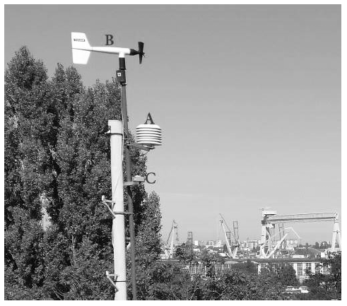
To register weather parameters the weather station designed by the Authors and installed on the roof of the building of Gdynia Maritime University was used. This station, shown in Fig.1, consists of 3 sensors measuring the ambient temperature, moisture, directions and speeds of the wind and power density of radiation, it also has the module LB-480 used to stockpile the measuring results. This data can be watched and analysed online from any place on the Earth thanks to the interface Ethernet with which the module LB-480 is equipped.
The module LB-480 assures the data access and settings with the use of the protocol http. The default home page contains the table with the running results of measurements. The page is refreshed automatically every second and contains the current results of measurements [10].
Fig. 1 Sensors of the weather station situated on the mast of the building of Gdynia Maritime University (A -thermo-hydrometer, B – the wind-gauge, C – the sensor of power density of the solar radiation)
In the paper [11] the influence of weather conditions on the operation of the selected photovoltaic panels is analysed. The weather station making possible measurements of values of the selected weather parameters on the ground of Gdynia Maritime University is described. The measured waveforms of power density of solar radiation and air temperature in the selected days are presented. The electrothermal transient analysis of the polycrystalline photovoltaic panel operating with the linear resistance load was conducted. The obtained results of calculations were presented and discussed. The problem of the influence of weather parameters on cooling conditions of the photovoltaic panels was pointed out.
Photovoltaic installation
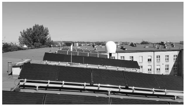
The photovoltaic system installed in Gdynia Maritime University is characterized by the installed top-power of silicon photovoltaic panels equal to 10.4 kWp. This system, shown in Fig. 2, is made according to the topology of the system SMA FLEXIBLE STORAGE SYSTEM based on the devices by SMA company including two network inverters of the type Sunny Boy 5000TL-21 operating in the two-phase-configuration and the insular inverter of the type Sunny Island 6.0H. In the considered system forty panels are used, each of the top-power equal to 260 kWp, including 20 monocrystalline panels – Axitec AC-260M/156-60S and 20 poly-crystalline panels – Axitec AC-260P/156-60S. The mounting construction of the panels makes possible manual regulation of the depression angle of these panels, which can be 20°, 35°, 50° or 60°.
The photovoltaic system provides electrical energy to the local energy-network installed in the laboratory of optoelectronics, photovoltaics and optical fibre technique.
Fig. 2. View of the photovoltaic installation in Gdynia Maritime University
The insular inverter makes possible the transformation of electrical energy of the direct current, aggregated in the battery of four gel batteries connected serially, characterised by the nominal voltage amounting to 12 V and the capacity of 220 Ah, into energy of the alternating current. The production of additional energy across the network inverter follows in the case of the too weak sun exposure (eg. large cloudiness, nighttime) and in the case of damage of the university energy-network. The communication between each device is realised across the local Internet network. Parameters of the system are sent to the Internet service Sunny Portal across the device of the name Sunny Home Manager. This service allows remote management with settings of the photovoltaic system and its monitoring.
Investigations results
With the use of the weather station presented in Section 2, weather parameters in the place of location of the photovoltaic installation described in Section 3 were measured and recorded. The measurements of weather parameters and exploitive parameters of the considered installation have been performed since October 2015.
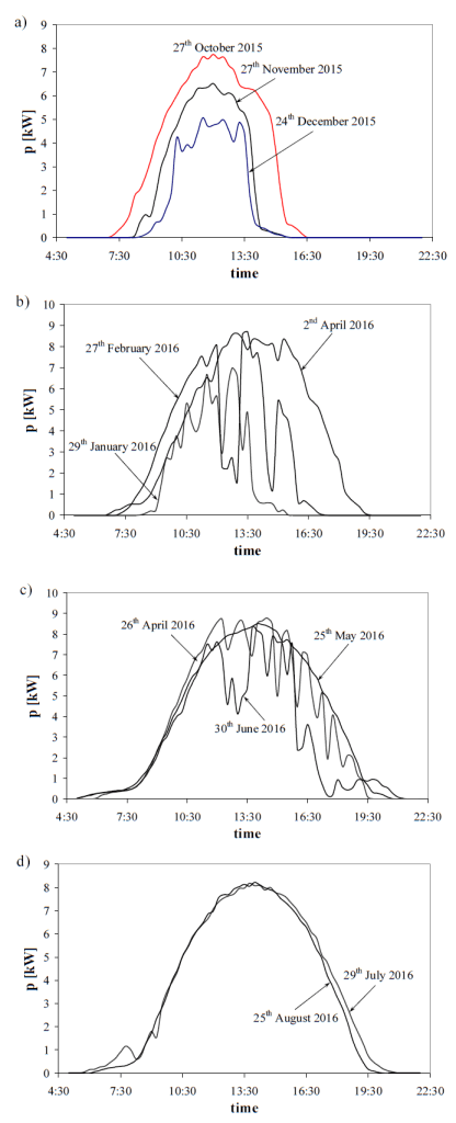
As an example, in Fig. 3 the measured courses of changes of power density of solar radiation during twenty-four hours are shown, and in Fig. 4 – the corresponding to them courses of power produced by the considered installation. For the presentation the Authors selected the arbitrarily data from the following days – 27th October 2015, 27th November, 24th December 2015, 29th January 2016, 27th February 2016, 2nd April 2016, 26th April 2016, 25th May 2016, 30th June 2016, 29th July 2016 and 25th August 2016.
As it is visible, the considered waveforms obtained for all the considered days have similar courses, and over the considered period of time the maximum power density of solar radiation in winter and in summer changes even four times. As a result of changing times of the sunrise and the sunset, as well as changes of the height of the sun over the horizon at noon, there are visible changes of the maximum value of pV and time, in which the values of pV are much more than zero.
In the considered curves obtained in the selected days many local minima and maxima are observed. These local extrema are a result of changes in cloudiness during the considered days. These changes cause fast changes in the value of power density of solar radiation. For example in the curve measured on 29th July 2016 it is visible that during 10 minutes only the value of pV decreases from 1100 W/m2 to 300 W/m2. On the other hand, for a sunny day the curve pV(time) has the shape near the Gaussian curve.
Fig. 3. Measured time distribution of power density of solar radiation
As it is visible in Fig. 4, the output power of the photovoltaic system visibly changes every day and during the year. It is worth noticing that the maximum output power of the photovoltaic system changes from about 5 kW in December to about 9 kW in June.
Fig. 4. Measured time distribution of the output power of the photovoltaic system
In the observed curves it is visible that the energy produced by the considered system depends on power density of solar radiation pV. Particularly, changes in values of pV (observed in Fig. 3) cause changes in the values of the output power of the considered system. The maximum value of the output power equal to the nominal value of this parameter was obtained in the period between April and October.
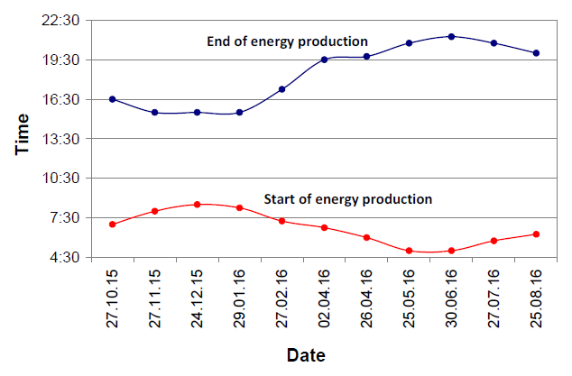
The information about time at which the power generation starts and stops in the considered days is presented in Fig.5.
Fig. 5. Time of starting and stopping energy generation by the photovoltaic system in the selected days
It is visible that this time is very short between November and January and its value is about only 7 hours, whereas in summer this time is equal to about 16 hours.
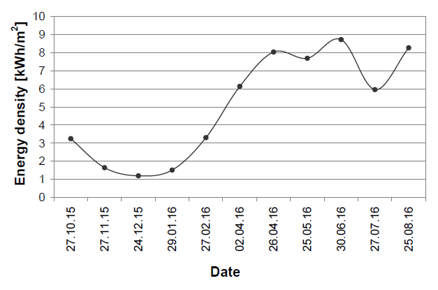
From the point of view of the user of a photovoltaic system information about electrical energy produced by this system is very important. The value of this energy depends on solar energy. In Fig.6 the values of solar energy density in the selected days are shown, whereas in Fig. 7 – the values of electrical energy produced by the considered system in the same days are presented.
Fig. 6. Solar energy density in the selected days
Fig. 7. Electrical energy produced by the photovoltaic system in the selected days
As it is visible, shapes of the curves shown in Fig. 4 and 5 are similar. The minimum value of the produced energy is observed in December and it is equal to 25% only of the value of this energy produced in May. The observed changes in the value of the produced electrical energy is twice smaller than changes in the value of density of solar energy. The value of electrical energy produced each day in the period from the beginning of April to the end of August is nearly the same and it is equal to about 60 kWh.
Conclusions
In the paper the investigations results of the photovoltaic installation and the weather station situated in Gdynia Maritime University are presented. The long-time investigations confirmed that the output power of the considered installation was not proportional to power density of solar radiation. It is also visible that changes of power density of solar radiation due, among other things to variable cloudiness get averaged. The energy produced by the considered installation changes even four times during the period from the end of December to the beginning of April and the time, in which energy is produced during this period, increases twice. During 5 months the value of the produced each day electrical energy is equal to its maximum.
REFERENCES
[1] D. Mulvaney, Solar’s Green Dilemma, IEEE Spectrum, No. 9, 2014, pp. 26-29 [2] J. Singh, “Semiconductor devices: basic principles”, John Wiley&Sons, 2000 [3] E. Klugmann-Radziemska, „Fotowoltaika w teorii i praktyce”, Wydawnictwo BTC, Legionowo, 2010. [4] L. Castaner, S. Silvestre, „Modelling photovoltaic systems using Pspice”, John Wiley&Sons, 2002. [5] M.H. Rashid, “Power Electronic Handbook”, Academic Press, Elsevier, 2007. [6] E. Krac, K. Górecki: Modelling characteristics of photovoltaic panels with thermal phenomena taken into account. IOP Conference Series: Materials Science and Engineering, Vol. 104, 2016, 39th International Microelectronics and Packaging IMAPS Poland 2015 Conference, 012013, pp. 1-7, doi:10.1088/1757-899X/104/1/012013. [7] W. Marańda, M. Piotrowicz: “Extraction of Thermal Model Parameters for Field-Installed Photovoltaic Module”, PROC. 27th International Conference on Microelectronics (MIEL 2010), NIŠ, Serbia, 16-19 MAY, 2010. [8] K. Górecki, J. Zarębski: Modeling the influence of selected factors on thermal resistance of semiconductor devices. IEEE Transactions on Components, Packaging and Manufacturing Technology, Vol. 4, No. 3, 2014, pp. 421-428 [9] F.F. Oettinger, D.L. Blackburn: Semiconductor measurement technology: thermal resistance measurements U. S. Department Commerce NIST/SP-400/86, 1990 [10] T Markvart, L Castañer Practical handbook of photovoltaics : fundamentals and applications; Oxford: Elsevier Advanced Technology, 2003 [11] http: //mk.label.pl/lb480-user-manual/pl/lb480-usermanual.pl.pdf [12] E. Krac, K. Górecki: The influence of selected weather parameters on characteristics of photovoltaic panels. Elektronika, No. 5, 2016, pp. 40-43
Autorzy: dr inż. Jacek Dąbrowski, mgr inż. Ewa Krac, prof. dr hab. inż. Krzysztof Górecki, Akademia Morska w Gdyni, Katedra Elektroniki Morskiej, ul. Morska 81-87, 81-225 Gdynia, E-mails: j.dabrowski@we.am.gdynia.pl, e.krac@we.am.gdynia.pl, k.gorecki@we.am.gdynia.pl
Source & Publisher Item Identifier: PRZEGLĄD ELEKTROTECHNICZNY, ISSN 0033-2097, R. 93 NR 2/2017. doi:10.15199/48.2017.02.44
Published by Anushree Ramanath, EE Power – Technical Articles: An Introduction to Microgrid Energy Management Systems, July 05, 2021.
This article highlights the growth of microgrids and the components of these systems.
With the growing number of industries and businesses, access to reliable and cost-effective power is critical. This leads to demand for small-scale power supply networks to cater to the communities. The microgrid thus formed serves as a connection between the power generation facility and the utility grid [1]. It enables resilience, reliability, energy efficiency, environmental benefits, and economic gains. This promises uninterrupted power, thus prevents outages, and manages energy loads of multiple generation systems along with storage systems. The management aspect of the microgrid is handled through dedicated software and control systems. Read on to learn more about what a microgrid is, how it works, and its pros and cons.
Microgrids are a growing segment of the energy industry and represent a paradigm shift from remote central power plants to more localized distributed generation [2]. The microgrid concept has been around for several years, but it has gained significant traction in recent years as many projects are put into production, turning the concept into reality. If we observe closely, we realize that the early power systems developed by Thomas Edison and Nikola Tesla were all essentially microgrids. They are known to be revolutionary as they act as new drivers supporting the expansion of electrification while reducing the carbon footprint and enabling new technologies to support clean energy endeavors.
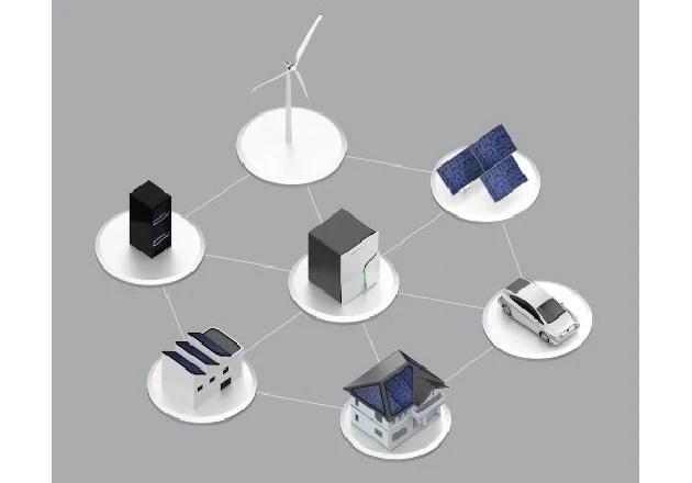
The microgrid is a local energy system capable of producing and distributing energy and is composed of different types of assets, also known as distributed energy resources (DERs), as illustrated in Figure 1. It can also be termed as a miniature power grid system that manages DERs, including both renewable and non-renewable sources of energy. It can be connected to the grid-like in healthcare facilities where continuous power is inevitable or be run entirely off the grid as it is self-sustaining in nature, like in remote sites that require tremendous amounts of energy.
Figure 1: Illustration of a microgrid [4]
The process of building a microgrid can be described as that of a Paladin lifecycle [3]. It involves the initial feasibility study of the site, the possible design, and the modeling of it. It is followed by the power study, including model-based studies, forecasting, and optimization. The next stage involves system design and management, including analysis of interconnection, implementation, and real-time simulations. The final step involves real-time control and optimization of all the power components.
Components of a Microgrid
The U.S. Department of Energy (DOE) defines a microgrid as “A group of interconnected loads and distributed energy resources within clearly defined electrical boundaries that acts as a single controllable entity with respect to the grid. A microgrid can connect and disconnect from the grid to enable it to operate in both grid and island modes” [5]. A microgrid generally comprises renewable or fossil-fueled generators, loads, energy storage systems, circuit breakers, and control equipment, as illustrated in Figure 2.
The most commonly employed assets to generate power are photovoltaics (PV), wind turbines, and power generators. The other elements critical in terms of the functionality of a microgrid include storage systems, smart controls, and software that facilitates interconnection. All of these components need to work well together to ensure a seamless customer experience while adhering to standard regulatory requirements.
Figure 2: Components of a microgrid [6]
Advantages of Microgrids
The formation of microgrids assures efficient and low-cost clean energy along with reducing grid congestion and peak loads. It helps improve the stability of the grid while enhancing the reliability and resilience of the critical infrastructure. It also helps in reducing the carbon footprint and line losses while promoting the use of renewable energy sources.
Microgrids offer several financial benefits, including tax breaks, discounts and avoid peak pricing burden. It is also diversified and produces energy from multiple sources like wind, solar, and fuel cells, adding several levels of security [3]. They come in handy as they are smaller and can be installed quickly than traditional power plants. Further, microgrids can integrate with the grid along with other smart grid technologies with ease.
Disadvantages of Microgrids
The main disadvantage of a microgrid is the resynchronization with the main grid.
There is also a need for ample storage, which again demands an additional cost, maintenance, and space for installation. There is some resistance from the utilities to implement microgrid technologies. There are also regulatory issues that might be difficult to comply with, and it is difficult for laws to catch up with building technology.
Author: Anushree Ramanath is a seasoned engineering professional skilled in system-level design, building hardware, coding, firmware, industry-oriented research, software architecture, modeling, and simulations. She received a Ph.D. in Electrical and Computer Engineering from the University of Minnesota Twin Cities with a focus on power and controls. She loves experiencing different cultures through languages, food, or travel while indulging in a variety of fine arts
Published by Electrical Installation Wiki, Chapter M. Power harmonics management – Solutions to mitigate harmonics
There are three different types of solutions to attenuate harmonics:
• Modifications in the installation • Special devices in the supply system • Filtering
Basic solutions to mitigate harmonics
To limit the propagation of harmonics in the distribution network, different solutions are available and should be taken into account particularly when designing a new installation.
Position the non-linear loads upstream in the system
Overall harmonic disturbances increase as the short-circuit power decreases.
All economic considerations aside, it is preferable to connect the non-linear loads as far upstream as possible (see Fig. M24).
Fig. M24 – Non-linear loads positioned as far upstream as possible (recommended layout)
Group the non-linear loads
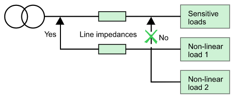
When preparing the single-line diagram, the non-linear devices should be separated from the others (see Fig. M25). The two groups of devices should be supplied by different sets of busbars.
Fig. M25 – Grouping of non-linear loads and connection as far upstream as possible (recommended layout)
Create separate sources
In attempting to limit harmonics, an additional improvement can be obtained by creating a source via a separate transformer as indicated in the Figure M26.
The disadvantage is the increase in the cost of the installation.
Fig. M26 – Supply of non-linear loads via a separate transformer
Transformers with special connections
Different transformer connections can eliminate certain harmonic orders, as indicated in the examples below:
• A Dyd connection suppresses 5th and 7th harmonics (see Fig. M27) • A Dy connection suppresses the 3rd harmonic • A DZ 5 connection suppresses the 5th harmonic
Fig. M27 – A Dyd transformer blocks propagation of the 5th and 7th harmonics to the upstream network
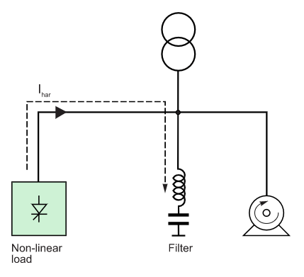
Install reactors
When variable-speed drives are supplied, it is possible to smooth the current by installing line reactors. By increasing the impedance of the supply circuit, the harmonic current is limited.
Installation of harmonic suppression reactors on capacitor banks increases the impedance of the reactor/capacitor combination for high-order harmonics.
This avoids resonance and protects the capacitors.
Select the suitable system earthing arrangement
TNC system
In the TNC system, a single conductor (PEN) provides protection in the event of an earth fault and the flow of unbalance currents.
Under steady-state conditions, the harmonic currents flow in the PEN. Because of the PEN impedance, this results in slight differences in potential (a few volts) between devices that can cause electronic equipment to malfunction.
The TNC system must therefore be reserved for the supply of power circuits at the head of the installation and must not be used to supply sensitive loads.
TNS system
This system is recommended if harmonics are present.
The neutral conductor and the protection conductor PE are completely separate and the potential throughout the distribution network is therefore more uniform.
Harmonic filtering
In cases where the preventive action presented above is insufficient, it is necessary to equip the installation with filtering systems.
There are three types of filters:
• Passive • Active • Hybrid
Passive filters
Typical applications
• Industrial installations with a set of non-linear loads representing more than 500kVA (variable-speed drives, UPSs, rectifiers, etc.) • Installations requiring power-factor correction • Installations where voltage distortion must be reduced to avoid disturbing sensitive loads • Installations where current distortion must be reduced to avoid overloads
Operating principle
An LC circuit, tuned to each harmonic order to be filtered, is installed in parallel with the non-linear load (see Fig. M28). This bypass circuit absorbs the harmonics, thus avoiding their flow in the distribution network.
Generally speaking, the passive filter is tuned to a harmonic order close to the order to be eliminated. Several parallel-connected branches of filters can be used if a significant reduction in the distortion of a number of harmonic orders is required.
Fig. M28 – Operating principle of a passive filter
Active filters (active harmonic conditioner)
Typical applications
• Commercial installations with a set of non-linear loads representing less than 500kVA (variable-speed drives, UPSs, office equipment, etc.) • Installations where current distortion must be reduced to avoid overloads.
Operating principle
These systems, comprising power electronics and installed in series or parallel with the non-linear load, compensate the harmonic current or voltage drawn by the load.
Figure M29 shows a parallel-connected active harmonic conditioner (AHC) compensating the harmonic current (Ihar = -Iact).
The AHC injects in opposite phase the harmonics drawn by the non-linear load, such that the line current Is remains sinusoidal.
Fig. M29 – Operating principle of an active filter
Hybrid filters
Typical applications
Industrial installations with a set of non-linear loads representing more than 500kVA (variable-speed drives, UPSs, rectifiers, etc.)
• Installations requiring power-factor correction • Installations where voltage distortion must be reduced to avoid disturbing sensitive loads • Installations where current distortion must be reduced to avoid overloads • Installations where strict limits on harmonic emissions must be met
Operating principle
Passive and active filters are combined in a single system to constitute a hybrid filter (see Fig. M30). This new filtering solution offers the advantages of both types of filters and covers a wide range of power and performance levels.
Fig. M30 – Operating principle of a hybrid filter
Selection criteria
Passive filter
It offers both power-factor correction and high current-filtering capacity. Passive filters also reduce the harmonic voltages in installations where the supply voltage is disturbed. If the level of reactive power supplied is high, it is advised to turn off the passive filter at times when the percent load is low.
Preliminary studies for a filter must take into account the possible presence of a power factor correction capacitor bank which may have to be eliminated.
Fig. M31 – Example of MV passive filter equipment
Active harmonic conditioners
They filter harmonics over a wide range of frequencies and can adapt to any type of load. On the other hand, power ratings are limited.
Fig. M32 – Active Harmonic Conditioner (AccuSine range)
Hybrid filters
They combine the performance of both active and passive filters.
The method to optimize harmonics mitigation
The best solution, in both technical and financial terms, is based on the results of an in-depth study.
Harmonic audit of MV and LV networks
By calling on an expert, you are guaranteed that the proposed solution will produce effective results (e.g. a guaranteed maximum THDu).
A harmonic audit is carried out by an engineer specialised in the disturbances affecting electrical distribution networks and equipped with powerful analysis and simulation equipment and software.
The steps in an audit are the following:
• Measurement of disturbances affecting current and phase-to-phase and phase-to-neutral voltages at the supply source, the disturbed outgoing circuits and the non-linear loads
• Computer modelling of the phenomena to obtain a precise explanation of the causes and determine the best solutions
• A complete audit report presenting:
– The current levels of disturbances – The maximum permissible levels of disturbances (refer to IEC 61000, IEEE 519, etc.)
• A proposal containing solutions with guaranteed levels of performance
• Finally, implementation of the selected solution, using the necessary means and resources.
The entire audit process should be certified ISO 9002.
Published by Electrical Installation Wiki, Chapter M. Power harmonics management – Harmonics standards
Harmonic emissions are subject to various standards and regulations:
• Compatibility standards for distribution networks • Emissions standards applying to the equipment causing harmonics • Recommendations issued by Utilities and applicable to installations
In view of rapidly attenuating the effects of harmonics, a triple system of standards and regulations is currently in force based on the documents listed below.
Standards governing compatibility between distribution networks and products
These standards determine the necessary compatibility between distribution networks and products:
• The harmonics caused by a device must not disturb the distribution network beyond certain limits
• Each device must be capable of operating normally in the presence of disturbances up to specific levels
• Standard IEC 61000-2-2 is applicable for public low-voltage power supply systems • Standard IEC 61000-2-4 is applicable for LV and MV industrial installations
Standards governing the quality of distribution networks
• Standard EN 50160 stipulates the characteristics of electricity supplied by public distribution networks
• Standard IEEE 519 presents a joint approach between Utilities and customers to limit the impact of non-linear loads. What is more, Utilities encourage preventive action in view of reducing the deterioration of power quality, temperature rise and the reduction of power factor. They will be increasingly inclined to charge customers for major sources of harmonics
Standards governing equipment
• Standard IEC 61000-3-2 for low-voltage equipment with rated current under 16 A • Standard IEC 61000-3-12 for low-voltage equipment with rated current higher than 16 A and lower than 75 A
Maximum permissible harmonic levels
International studies have collected data resulting in an estimation of typical harmonic contents often encountered in electrical distribution networks. Figure M23 presents the levels that, in the opinion of many Utilities, should not be exceeded.
Fig. M23 – Maximum admissible harmonic voltages and distortion (%)
Published by Ana Maria Blanco1, Britta Heimbach2, Bruno Wartmann2, Jan Meyer1, Marco Mangani2, Martin Oeschger2 1Institute of Electrical Power Systems and High Voltage Engineering, Technische Universität Dresden, Dresden, Germany 2Elektrizitätswerk der Stadt Zürich – EWZ, Zurich, Switzerland 1E-mail: ana.blanco@tu-dresden.de
24th International Conference & Exhibition on Electricity Distribution (CIRED), 12-15 June 2017. Session 2: Power quality and electromagnetic compatibility
Abstract: Modern wind parks usually consist of multiple individual turbines, which are connected to the grid using power electronic interfaces. Depending on their topology, they could be a source of distortion in the frequency range below 2 kHz (harmonics, interharmonics) and above 2 kHz (supraharmonics). Consequently, the assessment of the impact of wind parks on the voltage distortion in the network is an important issue. This study explains some of these issues based on extensive field measurements at a recently commissioned 12 MW wind park consisting of six turbines with full inverter (type 4) and a rated power of 2MW each. While the first part discusses the distortion characteristic of an individual turbine, the second part is dedicated to the wind park as a whole and its impact on the voltage distortion at the connection point. Based on the experiences from the project some recommendations for field measurements at wind parks are summarised.
1. Introduction
The number of wind parks is growing continuously. New park installations usually utilise turbines either of type 3 (Doubly-fed induction generator (DFIG)) or type 4 (full converter). As both of them include power electronic converters, their possible network impact with respect to harmonics is an important concern for manufacturers, planners, operators and utilities. According to current practice in most cases, emission limits in terms of harmonic current magnitudes are provided by the utility, and the planner has to confirm compliance, which is mostly done by simplified calculations. Dependencies of harmonic currents on output power, network impedance or supply voltage distortion as well as the real impact on the voltage harmonic levels in the network are in many cases not adequately considered yet. Experiences have shown that simulation based on estimations can suffer from high uncertainties and the impact assessment based only on currents might be insufficient, as it does not consider possible cancellation effects with the existing supply voltage distortion (background distortion) properly.
Several studies exist, which analyse the harmonic and interharmonic currents of wind parks and the aggregation characteristic of multiple turbines based on field measurements [1–3]. This paper aims to contribute to these research activities and discusses some aspects of the current distortion within a typical wind park installation as well as its impact on the voltage distortion at the connection point with the grid.
After a short description of the wind park layout, the measurement campaign is explained. This includes also a brief discussion of issues related to the measurement uncertainties of the used sensors and instrument transformers. The next part presents selected results for individual turbines (units), while the last part is dedicated to the harmonics at installation level. Based on the experiences from the measurement campaign the paper concludes with some general recommendations.
2. Measurement campaign
The wind park consists of six similar type four turbines and has a total rated power of 12 MW. The park is connected to a 110 kV/ 20 kV substation via a 23.5 km MV cable. Two types of measurements have been performed:
• A long-term measurement of almost 2 months in order to monitor the typical behaviour of harmonics under typical operating conditions.
• A short-term measurement where turbines have been actively controlled according to a defined schedule in order to identify the impact of specific operating conditions on harmonic distortion.
Measurements have been performed at each turbine using six GPS synchronised IEC 61000-4-30 class A power quality analyser with a frequency range up to 10 kHz and the additional capability to measure absolute harmonic phase angles. In addition, a transient recorder with a sampling rate of 1 MS/s has been used for acquiring highly synchronised data of the feeders and the complete wind park during the short-term measurements. The location of the instruments is shown in Fig. 1.
For each instrument/sensor combination individual accuracy thresholds have been identified based on a procedure introduced in [4]. Above the threshold, the measurement uncertainty at all considered frequencies is better than 10%/5°. The obtained thresholds are summarised in Table 1.
All measurement data below the threshold have been excluded from the analysis. It should be noted that especially the accuracy of harmonic phase angles has a high impact on the analysis of harmonics summation and cancellation effects [5].
Fig. 1 Layout of the wind park and measurement instruments
Table 1 Accuracy thresholds of the measurement instruments
.
3 Analysis at turbine level
3.1 Magnitude/level of distortion current
Fig. 2 presents exemplarily the harmonic, interharmonic and supraharmonic currents for the wind turbine Wind turbine generator (WTG1) (dots). According to IEC 61000-4-7 harmonics and interharmonics have been measured as subgroups and supraharmonics as 200 Hz bands. The aggregation interval has been set to 10 min and root mean square (RMS) method has been applied for aggregating the 10 cycle values as defined in IEC 61000-4-30. Each dot represents the maximum value observed during the long-term measurement interval taking only values when the turbine operated between 90 and 100% of its rated output power. The grey bars represent the equivalent values reported by the respective manufacturer certificate according to IEC 61400-21.
The most significant harmonic currents are the 5th, 7th, 11th and 13th (Fig. 2, left). Related to the rated current of the turbine these values are well below 1%, most of them even below 0.5%. The dominating share of harmonics matches the certificate values reported by the manufacturer. However, for several harmonic orders significant differences in both directions (higher/lower than certificate values) can be observed. The main reason for these differences is that the total measured current is a combination of two parts: one part caused by the turbine itself and one part caused by the network due to the supply voltage distortion. According to [6] the first part can be referred to as primary emission, the second part as secondary emission. Deviations in supply voltage distortion as well as deviations in the network harmonic impedance between the test facility for certification measurements and the connection point cause the observed differences. Consequently, the simple comparison of measured harmonic currents with specified limits is often not sufficient and it might result in misleading conclusions. It can be further noted that for some orders the harmonic current is unbalanced, which is most likely caused by a slight unbalance in background distortion.
The highest levels for interharmonic currents (Fig. 2, middle) are obtained at order 2 and around order 15. Related to the rated current of the turbine these currents are below 0.25%. Most of the levels match the certificate values of the manufacturer well, because no significant interharmonic background distortion exists.
The supraharmonic currents in the frequency range 2–9 kHz are well below 0.1% in relation to the rated current of the turbine. Most of the measured levels show a significant difference to the certificate values, being usually lower. This behaviour confirms the often reported fact that the distortion above 2 kHz depends much more on the connection point characteristic than the distortion below 2 kHz [8]. Especially the impedance at higher frequencies is more volatile as it is mainly determined by the equipment connected nearby.
Fig. 3 compares the harmonic, interharmonic and supraharmonic currents of one phase between all six turbines. In spite of slight differences, the turbines in general behave very similar. This applies also for the other phases. The differences are caused by slight differences in the voltage distortion, output power and/or control settings of each turbine as well as differences in the circuit elements (inverter, filter, transformer etc.).
Fig. 2 Harmonic (left), interharmonic (middle) and supraharmonic (right) currents (dots: measured values; bars: values provided by manufacturer)
Fig. 3 Maximum harmonic (left), interharmonic (middle) and supraharmonic (right) currents of all turbines (phase A)
3.2 Prevailing harmonic phase angles
In order to determine the similarity between the individual turbines, not only the magnitude, but also the phase angles of distorting currents have to be considered. In general, two different options exist for the calculation of the phase angle: phase angle between voltage and current at the same frequency (relative harmonic phase angle; e.g. for harmonic power flow studies) and phase angle between harmonic current and fundamental voltage (absolute harmonic phase angle). The absolute harmonic phase angle is often referred to as prevailing phase angle. It is used to study cancellation effects between the harmonic currents of individual devices (also referred to as primary cancellation) as well as between the harmonic current of an installation and the existing background voltage harmonics (also referred to as secondary cancellation). Further details about primary and secondary cancellation can be found in [7]. This paper discusses harmonic cancellation effects and consequently applies the absolute harmonic phase angle.
The level of similarity (or steadiness), also referred to as the level of prevalence of the harmonic phase angle for multiple measurement data i (e.g. in a certain time interval) is determined based on the complex harmonic currents Ii(h)by the harmonic prevailing ratio PR(h):
.
As an example Fig. 4 (left) presents all data points of the long-term measurement for the seventh current harmonic and all three phases of turbine WTG1 in the complex plane. The dispersion is caused by the supply voltage distortion as well as the varying operating points of the wind park. A prevailing location can be identified in the heat map plot (Fig. 4, right) as red area, which corresponds to the area of highest density of measurement data.
Fig. 4 Example of the prevailing phase angle and prevailing ratio for the 7th harmonic current of turbine WTG1 (phase A)
The prevailing phase angle of a set of data points is calculated by
.
If the data is too dispersed (usually for PR(h) < 0.8), the prevailing phase angle has no meaning and should not be reported. Further explanations on calculation and assessment of harmonic cancellation effects and prevailing ratio can also be found in [7]. Table 2 exemplarily presents the prevailing phase angles for the first two turbines WTG1 and WTG2 (cf. Fig. 1) and the first nine harmonics for the long-term measurements. The colours indicate the level of prevalence. The other turbines behave similar. Considering the whole long-term measurement, in most cases the dispersion of harmonic phase angles is high. Only 2nd, 4th and 7th harmonic orders present a consistent and distinctive prevalence. This confirms the high sensitivity of harmonic currents on the operating conditions of the wind park and that simple constant current source models are not sufficient for developing accurate models for harmonic studies.
Table 2 Prevailing phase angle in degree for turbines WTG1 and WTG2
.
3.3 Impact of supply voltage distortion
Output power and supply voltage distortion are the most significant factors influencing the resulting distortion current of a wind park installation. It is expected that output power mainly determines the primary emission, while supply voltage distortion causes mainly secondary emission depending on the frequency dependent input impedance of the turbines. In field measurements both factors usually fluctuate at the same time and methods to distinguish the influences of both factors are required. This section introduces a method to separate the impact of supply voltage distortion (background distortion) on distortion currents in field measurements and to identify if a linear relation exists between them.
All data of the long-term measurement are divided into a matrix of 25 × 25 ‘cells’ with approximately the same output power (Fig. 5, left). Active and a reactive output power ranges of each cell are determined by dividing the maximum active and reactive power observed during the measurement interval by 25. Next, the correlation coefficient c according to Pearson is calculated individually for each harmonic order and each cell. A correlation coefficient in the range between 0.8 and 1.0 indicates a strong linear relationship. Fig. 5(right) exemplarily shows the correlation between the 5th voltage and current harmonic magnitudes for one cell with very strong linear correlation.
Fig. 5 Example of power cell grid (right) and detailed data correlation analysis for cell {7,5} and 5th harmonic, phase A
A colour map plot of the correlation coefficients allows an easy visual assessment of existing linearity. As an example, Fig. 6 shows the colour map obtained for the correlations between the voltage and current harmonics for the 7th harmonic of phase A at turbine WTG3. White cells indicate that no or not enough measurement data are available for analysis. Comparing the results of all turbines and all phases it was found that strong linear correlations exist for a dominating share of ‘cells’ for the 5th, 7th, 11th, 13th, 14th, 15th and 16th harmonic orders, which are the most dominant harmonics (Fig. 2, left). Particularly at higher reactive power output correlation seems to be usually weaker. It should be noted that a low correlation coefficient only means that no linear correlation exists, but not that no correlation exists at all.
Fig. 6 Correlation coefficients for 7th harmonic, phase A, turbine WTG3
4. Analysis at wind park level
Selected aspects of the total harmonic and interharmonic currents of the wind park and its impact on the voltage distortion at the connection point are exemplarily discussed using a part of the short-term measurements, where the active output power of the wind park has been increased stepwise from 1 to 9 MW, while reactive power has been kept constant at Q=0.
Most relevant harmonic currents (Fig. 7/top) do not show a consistent behaviour during the test. While some of them increase with increasing active output power (e.g. 3rd and 7th), others remain nearly constant (e.g. 8th and 10th). Some harmonic currents seem to decrease again slightly at higher active output powers (e.g. 2nd and 11th). Harmonic voltages (Fig. 7/bottom) are very low and in general do not increase during this test. Slight variations (e.g. for 5th harmonic) are most likely caused by fluctuations of the existing background distortion during the test (about 40 min), because such fluctuations do also affect the harmonic currents (secondary emission). Only the 7th harmonic voltage shows a clear, decreasing trend. As the 7th harmonic current increases at the same time (indirect relation), a certain level of cancellation exists between the background harmonic voltage and the voltage drop at the network impedance caused by the 7th harmonic current of the wind park. This type of cancellation is also referred to as secondary cancellation (to subsection prevailing harmonic phase angles). The polar plots in Fig. 8 confirm this explanation, as the 7th voltage harmonic considerably changes its phase angle with increasing harmonic current. Further details and a method for a simplified assessment of the level of secondary cancellation can be found in [7].
Interharmonic currents (Fig. 9) consistently increase with increasing active output power. This characteristic also applies to the higher interharmonics, which are not shown in the figure. Interharmonic voltages are very low and increase with increasing interharmonic currents. The level of increase is partly linked to the network impedance. As virtually no interharmonic background voltages exist, secondary cancellation effects like for the 7th harmonic do consequently not occur.
Fig. 7 Harmonic currents and voltages (99%). (Bars indicate from left (blue) to right (yellow) different active output power levels (MW): 1.1, 2.3, 3.5, 4.5, 6.0, 7.0, 8.0, 9.0
Fig. 8 Seventh harmonic current (left) and voltage (right); colours indicate different output power levels (black: 1.1 MW, light red: 9 MW)
Fig. 9 Interharmonic currents and voltages (99%). (Bars indicate from left (blue) to right (yellow) different active output power levels (MW): 1.1, 2.3, 3.5, 4.5, 6.0, 7.0, 8.0, 9.0
5. Summary
The paper discusses some aspects of the distortion characteristic of a 12 MW wind park consisting of six similar turbines based on field measurements. Distortion covers harmonics and interharmonics below 2 kHz as well as distortion above 2 kHz (supraharmonics). A statistical analysis of the typical distortion characteristic is based on long-term measurements at reference/default settings of the wind park and the turbines. The impact of different operating points or changes of parameter settings on the distortion characteristic is analysed based on short-term measurements performing different sets of ‘controlled’ tests (e.g. change of output power). Furthermore, the analysis distinguishes between the characteristics of individual turbines and the park installation as a whole.
The individual turbines behave similar, but differ partly to the distortion current values provided by the manufacturer certificate. This confirms that location-specific conditions, particularly frequency-dependent network impedance and supply voltage distortion have a significant impact on the distortion currents. The analysis at wind park level shows that, especially in case of harmonics, currents can also have a positive impact on the voltage distortion in the network. Particularly where harmonic currents exceed specified limits, it is recommended to assess this impact before considering additional mitigation equipment. This issue is also discussed in the joint CIGRE/CIRED working group C4.42. Last but not the least, it should be mentioned that during the long-term measurements the voltage quality at the connection point did fully comply with EN 50160.
Within the project, a huge amount of data has been collected. A fundamental basis for any further analysis is a careful determination of measurement accuracy, which includes all external sensors. A set of existing as well as newly developed methods have been applied to analyse different aspects of the distortion characteristic of the individual turbines and the wind park. However, a modular framework for measurement and analysis of the distortion characteristics of a customer installation is still missing and should be developed in the future.
6. References
1. Yang, K., Bollen, M., Wahlberg, M.: ‘A comparison study of harmonic emission measurements in four windparks’. IEEE Power and Energy Society General Meeting, IEEE, 2011 2. Yang, K., Bollen, M., Larsssson, A.: ‘Aggregation and amplification of wind-turbine harmonic emission in a windpark’, IEEE Trans. Power Deliv., 2015, 30, (2), pp. 791–799 3. Van Reusel, K., Bronckers, S.: ‘Summation rule for wind turbines’ harmonics challenged by measurements’. 17th Int. Conf. on Harmonics and Quality of Power, 2016 4. Meyer, J., Kilter, J.: ‘Case studies for power quality monitoring in public distribution grids – some results of working group CIGRE/CIRED C4.112’. Electric Power Quality and Supply Reliability Conf., 2014 5. Blanco, A.M., Meyer, J., Schegner, P.: ‘Calculation of phase angle diversity for time-varying harmonic currents from grid measurement’. Int. Conf. on Renewable Energies and Power Quality, 2014 6. Bollen, M.H.J., Rönnberg, S.K.: ‘Primary and secondary harmonics emission; harmonic interaction – a set of definitions’. 17th Int. Conf. on Harmonics and Quality of Power, 2016 7. Meyer, J., Bollen, M., Amaris, H., et al.: ‘Future work on harmonics – some expert opinions Part II – supraharmonics, standards and measurements’. 16th Int. Conf. on Harmonics and Quality of Power, 2014 8. Meyer, J., Blanco, A.M., Domagk, M., et al.: ‘Assessment of prevailing harmonic current emission in public low voltage networks’, IEEE Trans. Power Deliv., 2017, 32, (2), pp. 962–970
Source & Publisher Item Identifier: CIRED, Open Access Proc. J., 2017, Vol. 2017, Iss. 1, pp. 677–681, ISSN 2515-0855, doi: 10.1049/oap-cired.2017.0457
Published by Paweł A. MAZUREK, Lublin University of Technology, Institute of Electrical Engineering and Electrotechnologies
Abstract. The effectiveness of measures to improve the quality of electricity and the electromagnetic compatibility of electrical equipment is linked to limiting the disturbances introduced by receivers to the power grid and depends on the identification of such interference. The paper presents the results of examining several popular receivers based on power electronics
Streszczenie. Skuteczność działań dotyczących poprawy jakości energii elektrycznej i kompatybilności elektromagnetycznej urządzeń elektrycznych jest związana z ograniczaniem zakłóceń wprowadzanych przez odbiorniki do sieci elektroenergetycznej oraz uzależniona od identyfikacji tych zakłóceń. W pracy przedstawiono wyniki badań w torze zasilania kilku popularnych odbiorników bazujących na energoelektronice. (Wybrane zagadnienia pracy urządzeń elektrycznych w odniesieniu do jakości energii i EMC).
Słowa kluczowe: jakość energii, kompatybilność elektromagnetyczna. Keywords: quality of energy, electromagnetic compatibility.
Introduction
In recent years we have seen a dynamic growth in the number of receivers in use, as well as in the changes occurring in their structure, which translates into troublesome effects of voltage distortion in the power grid. One reason is a significant increase in the number of receivers with power electronic input circuits that convert alternating current electricity into energy with other parameters than the mains. Such devices allow to reduce electricity consumption, but at the same time bring to the grid disturbances that distort the signal voltage (at deformed currents, higher harmonics are identified in the spectral distribution).
From the point of view of the user of electricity it is desirable to ensure continuity of supply and a voltage of constant frequency, effective value and perfectly sinusoidal waveform. Yet many phenomena depreciate the quality of energy. Thus waveform deformations are caused by consumers, and are associated with the working conditions of receivers, their operating principle or construction. With the increase in the number of devices causing disturbances, more and more equipment becomes sensitive to them. Work on improving the quality of electricity is basically related to the reduction of noise introduced by receivers to the power grid, and thus their electromagnetic compatibility.
The disruption in the voltage and current waveforms in electricity grids require research on electricity receivers. Such studies include the impact of noise on the correct operation of receivers and receiver impact on the power grid, i.e. emission of interference to the power grid. There is thus justification for the need for continuous research on receivers regarding both the basic parameters of power frequency (analysis of the shape of the momentary waveforms of voltage and current, harmonic content) and the frequency range of 9kHz-30MHz.
Requirements for power quality and electromagnetic compatibility
Monitoring of the quality level of electricity is still of interest to groups of scientists conducting research in the field of electricity generation and distribution, but more often is the practice of engineers in grid plants, with manufacturers, industrial and institutional customers, and even with individual customers. This is particularly important in the era of the development of distributed energy based on renewable energy sources. Electricity has become a commodity, and therefore must have its quality evaluated.
By definition (following the Advisory Committee on Electromagnetic Compatibility ACEC) power quality is a set of parameters describing the properties of the process of supplying energy to the user under normal operating conditions, determining continuity of supply (short and long power outage) and characterised by the supply voltage (value, asymmetry, frequency, waveform).
The quality of electricity is thus characterised by specific figures and ratios. The documents governing the basic issues related to power quality include Energy Law [1], Polish Standard PN-EN 61000-4-30 Electromagnetic compatibility (EMC) – Methods for testing and measurement – Methods for measuring the quality of energy, Polish Standard PN-EN 50160 [5], and the Regulation of the Minister of Economy and Labour of 20 December 2004 on detailed conditions for the operation of the power system setting out the quality standards of customer service and the technical parameters of power supply in the national power system. In relation to the MV and LV networks they are consistent with the values contained in the basic standard EN 50160. The legislative support in the area of power quality in the power system also includes other legal acts [3,4,5].
Supply voltage quality tests rely on the registration in good time of parameters determining the quality and after analysing the results, comparing them with the limit values contained in industry standards and regulations [8].
In accordance with current regulations in our country, all producers of electrical and electronic equipment must comply with the requirements defined in the EU directives including: the Machinery Directive, Low Voltage and EMC Directive [2]. According to the Electromagnetic Compatibility Directive a device should meet the requirements contained in the dedicated set of technical standards. There are two aspects of product evaluation. The first type of tests are measurements of emissions disorders. They give knowledge that the device does not cause interference with other equipment. The second type of research is the study of device resistance to disorders. Thus, by definition, electromagnetic compatibility means the ability of a device to satisfactorily operate in an electromagnetic environment without causing excessive electromagnetic disturbances to other equipment in that environment. This environment is also the supply system – thus disorders generated and propagated at high frequencies may affect the quality of energy.
Essential requirements of the emission of electromagnetic disturbances and immunity to electromagnetic interference are contained in Directive 2004/108/EC relating to electromagnetic compatibility (EMC) [2], as implemented into Polish law by the Act of 13 April 2007 on Electromagnetic Compatibility (Dz. U. [Journal of Laws of the Republic of Poland] 2007, No. 82, item. 556).
Specific requirements, or acceptable limits for electromagnetic emissions or evaluation criteria of the tests for electromagnetic immunity can be found among norms harmonised with the EMC directive [6,7]. Equipment complying with the EMC directive for conducted interference must generate electromagnetic emissions set inside the respective ranges. Permissible limits depend on the purpose of the device and are dedicated to the home, office or lightly industrialised (Class B) user or for use in industrial environments (Class A).
Measurements
The quality of electricity in the power system depends on the characteristics of the connected and used electricity receivers. A particular impact on the degree of degradation of the quality of electricity are non-linear receivers, on the one hand high-power appliances (mining and metallurgical), on the other thousands of low-power mass use devices, e.g. energy-efficient lighting, computers, impulse chargers). Non-linear receivers are complex technological devices generating a continuous spectrum of current harmonics causing distortion, voltage fluctuations and generating disturbances in the band of conducted radio interference. On the other hand, recent advances in power electronics introduce broadly understood improvement in the quality of electricity.
Energy quality refers to the standard supply voltage parameters that characterise the level of a specific disorder which causes a change in the ideal voltage waveform. Acceptable values of quality parameters are specified in PN-EN 50160 [5]. The study was conducted in the laboratory of the Institute of Electrical Engineering and Electrotechnology and completed in two stages. In the first part, tests were made using a power quality analyser, the second part focused on measuring interference. The study involved 3 laptops (Dell Vostro 3360, Dell Vostro 3560, HP Pavilion dv6899ew with the original power supply), energy saving lamps (N3PY15 15W, N3PY11 11W, CE3UT4 18W, Econ Twister 8W), ULTRAGLISS FV4350 iron and two CPU Desktops (with power adapters ATX-230P and FEEL LC- 8300ATN). Such an inspection list of receivers is a good representation of a typical range of devices in a typical household.
Most of the parameters to be evaluated are recorded as samples averaged during certain periods of time. Legislation [5] contains the maximum permissible deviations of specified parameters from the nominal values of each parameter on a weekly basis.
Fig.1. Photos from the study of power quality, a view of the PQM700 meter
For the measurement, recording and analysis of the supply power parameters the PQM-700 Sonel meter was used. The analyser fully complies with the requirements of the class S PN-EN 61000-4-30:2011. The meter is equipped with wires attached directly to the power supplying the voltage measurement point. For measuring currents a measurement clamp is used (in the tests it was type F5 current clamp). The analyser used allows to measure and record the parameters of supply voltage, effective current, current and voltage peak coefficients, mains frequency, power and energy, current and voltage component harmonics (up to the 40th), the current and voltage THD harmonic distortion coefficient, power factor, cosφ, tgφ. The full capabilities of the device are achieved with the “SONEL Analysis” dedicated software. The stand was assembled according to the scheme set out in Figure 2.
Fig.2. Block diagram for the measurement of power parameters
The following figures present screenshots of the Sonel Analysis program (Fig. 3, 4, 5) with values for selected receivers tested.
Fig.3. List of the power parameters of the PQM-700 analyser – the spectrum of current harmonics of 6 energy saving lamps working together
Fig.4. Voltage (blue/sinusoidal) and current (red/distorted signal) waveforms of 6 energy-saving bulbs studied together
Fig.5. Voltage (blue/sinusoidal) and current (red/distorted signal) waveforms of two desktops working together
Deformations of the voltage and current curve (higher harmonics) are among the adverse events occurring in electricity grids. They can cause disturbances in the network, usually involving the increase of power losses in the individual components, such as transformers or lines powering the recipients. Additional power losses directly affect the temperature rise in line wires, particularly the neutral line, which is important in the case of cable lines, resulting in faster aging of the insulation. Additional power dissipation in the windings of the transformers can in some cases lead to their overload or even damage. Receivers particularly sensitive to the presence of higher harmonics in voltage are also engines and capacitors. Higher harmonics give rise to parasitic moments in the motor windings, which may hinder its start-up and proper operation. Deformation of currents and voltages also interfere with the work of gauging instruments or security measures [10].
According to the Regulation of the Minister of Economy of 4 May 2007 on detailed conditions for the operation of the power system [3] (Dz. U. [Journal of Laws of the Republic of Poland] of 29 May 2007.), entities included in the connection group I-II are granted acceptable relative voltage values expressed as a percentage of the fundamental harmonic. The total harmonic distortion as a percentage (THDU%) calculated for harmonics up to the order of 40 cannot be greater than 8%. Because the cause of supply voltage distortions are deformed currents, in order to prevent the passage of current higher harmonics to the power system and reduce the risk of fire active higher harmonic filters are used.
Currents consumed by devices containing electronic converters are heavily distorted (have a significant THD ratio and strongly deformed course), depend on the type of rectifier used at the input, the way they are controlled and the type of converter load (its power, character, load variability in time). The current massive use of power converters in IT, electronic, industrial and lighting devices is causing distortion of the current drawn by such equipment, thus being a source of higher harmonics [8,10]. The results obtained indicate that the greatest deformation of the course is to be found in the circuit powering energy-saving light bulbs and desktop computers, and the lowest – an iron and laptop adapters.
The second stage of research were tests conducted to define the value of the conducted emission generated by consumer devices. This also requires appropriate methods and measuring devices.
The test stand is based on the Rohde&Schwarz ESCI3 measuring receiver and the NNB 41C Line Impedance Stabilisation Network. The system was powered by a dedicated circuit grid, according to the diagram in Figure 6. The disorder measurement boiled down to determining the UE voltage present at the input of the interference meter. Measurement stands for analysis of conducted interference do not require location in a shielded room, but in order to stabilise the measurement conditions a reference plane is used which is a 2×2 m grounded metal plate. In the measurements an interference meter was used (also known as a measuring receiver complying with the requirements) and an additional device, an artificial network, which represents a defined load impedance for the disturbance value. The artificial network stabilises the conditions of voltage disruption measurements in the power supply circuit of the object tested.
Fig.6. The block system for measuring disorders with line impedance stabilization network
The whole test was managed automatically by the EMC32 program. The sweeping settings were automatic, in accordance with CISPR16, sampling time was 7 ms, the measurement was carried out in the 150 kHz – 30 MHz band and included disorder detection at L1 and N. The analysis involved the same equipment as in the case studies of power quality: iron, laptops, CPUs of desktop computers and a set of energy-saving bulbs. According to the procedure for determining the compatibility of electrical devices/installations the disturbance values measured are compared with respective limits.
The test results obtained were compared with the limits. Selected values are collected on charts compiled in Figures 7 and 8. All the values presented were measured with an average value detector and were referred to the limiting average value. In the case of the desktop computer graph a linear axis was used in order to better illustrate the overrun.
Fig.7. The measured values of conducted disturbances in the power supply circuit of 6 energy-saving lamps, range 150kHz- 30MHz, AV detector, the orange line marks measurement in phase L1, the blue line – measurement in N, limit according to EN55022
The measurements clearly identified the levels of conducted disturbances. Qualitatively disturbances in the phase and neutral wires are similar.
Fig.8. The measured values conducted disturbances in the power supply circuit of two desktop computers, 150kHz-30MHz, AV detector, the orange line marks measurement in phase L1, the blue line – measurement in N
In all devices manufactured today, emission levels have a good supply compatibility (iron, laptops, energy-saving light bulbs – Figure 7). Only desktop PCs over several years old have exceed acceptable levels – Figure 8.
Conclusions
In recent years there has been a continuous increase in the number of devices and systems susceptible to various types of electromagnetic disturbances, among which are the supply voltage distortion. This makes the issue of power quality and the installation of receivers the subject of active measures of a legislative and technical nature. In addition, the development of distributed systems using renewable energy sources with variable capacity, leads to a situation where both the energy source and the receivers are treated as nonlinear objects.
The presence of harmonics and disorders of higher frequencies is a potential problem for the operation of a supply network, as well as the correct operation of devices connected to the network – lack of electromagnetic compatibility may result in the danger of exploitation of other objects or systems.
It is thus important to work on the development of methods for location of sources of harmonic currents and voltages in the power system as well as methods of selecting the optimal compensation and filtration. Issues of power quality and reliability of power supply are addressed in a lot of scientific and technical publications [8,9,10,11], and a summary of the current state of knowledge in this field is a number of issued legal acts, defining, among others, permissible deviations from the nominal values describing electricity.
The measurements carried out by the author in an actual power network with attached to it selected devices permit to specify the parameters that characterise power quality, taking into account the EMC requirements.
On the energy market conducted disturbances as well as harmonics are bi-directional in nature. At the connection point for power reception the liability for distortions or disturbances may lie both with the energy supplier and the recipient. It is therefore particularly important that the equipment or installations put on the market were fully adapted to the applicable requirements defined by the directive on electromagnetic compatibility, and hence safe for the natural and working environment.
LITERATURA
[1] Ustawa z dnia 10 IV 1997 r. – Prawo energetyczne. Dziennik Ustaw z 1997, nr 54, poz. 348 [2] Directive 2004/108/EC of the European Parliament and of the Council of 15 December 2004 on the approximation of the laws of the Member States relating to electromagnetic compatibility and repealing Directive 89/336/EEC L 390/24 Official Journal of the European Union EN, 31.12.2004 [3] Rozporządzenie Ministra gospodarki z dnia 4 maja 2007 r. w sprawie szczegółowych warunków funkcjonowania systemu elektroenergetycznego, dziennik Ustaw Nr 93, poz. 623, z dnia 29.05.2007 [4] Rozporządzenie ministra gospodarki i pracy z dnia 20 grudnia 2004 r. w sprawie szczegółowych warunków przyłączenia podmiotów do sieci elektroenergetycznych, ruchu i eksploatacji tych sieci. Dz.U. 2005 nr 2, poz. 6 [5] PN-EN 50160:2002, Parametry napięcia zasilającego w publicznych sieciach rozdzielczych [6] PN-EN 61000-2-4. Kompatybilność elektromagnetyczna. Środowisko. Poziomy kompatybilności dotyczące zaburzeń przewodzonych małej częstotliwości w sieciach zakładów przemysłowych. [7] PN-EN 61000-4-30:2011 – Kompatybilność elektromagnetyczna (EMC) – Metody badań i pomiarów –Metody pomiaru jakości energii [8] Barlik R., Nowak M.: Jakość energii elektrycznej – stan obecny i perspektywy, Przegląd Elektrotechniczny R. 81 NR 7-8/2005 [9] Mazurek P. A, Wac-Włodarczyk A., Serwin S., Błażejewska A.: Ocena przewodzonych zagrożeń elektromagnetycznych prototypowej spawarki inwertorowej, Przegląd Elektrotechniczny, 2012, nr 12b, vol. 88, s. 198-200 [10] Pawlęga A.: Problemy oceny jakości energii elektrycznej w miejscach jej dostarczania do odbiorców, Przegląd Elektrotechniczny, R.LXXIX 11/2003, 805÷810 [11] Dróżdż T., Kuciński S., Electromagnetic distortion test of renewable energy sources, Zeszyty naukowe Wyższej Szkoły Zarządzania Ochroną Pracy w Katowicach, Nr 1(9)/2013, s.5-14
Autohr: dr inż. Paweł A. Mazurek, Lublin University of Technology, Institute of Electrical Engineering and Electrotechnologies, ul. Nadbystrzycka 38a, 20-618 Lublin, E-mail: p.mazurek@pollub.pl.
Source & Publisher Item Identifier: PRZEGLĄD ELEKTROTECHNICZNY, ISSN 0033-2097, R. 93 NR 1/2017. doi:10.15199/48.2017.01.06