Published by Electrical Installation Wiki, Chapter M. Power harmonics management – Main effects of harmonics in electrical installations
Effects of harmonics – Resonance
The simultaneous use of capacitive and inductive devices in distribution networks may result in parallel or series resonance.
The origin of the resonance is the very high or very low impedance values at the busbar level, at different frequencies. The variations in impedance modify the current and voltage in the distribution network.
Here, only parallel resonance phenomena, the most common, will be discussed.
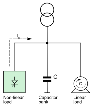
Consider the following simplified diagram (see Fig. M14) representing an installation made up of:
• A supply transformer, • Linear loads • Non-linear loads drawing harmonic currents • Power factor correction capacitors
Fig. M14 – Diagram of an installation
For harmonic analysis, the equivalent diagram is shown on Figure M15 where:
Ls= Supply inductance (upstream network + transformer + line) C = Capacitance of the power factor correction capacitors R = Resistance of the linear loads Ih= Harmonic current
Fig. M15 – Equivalent diagram of the installation shown in Figure M14
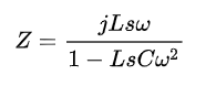
By neglecting R, the impedance Z is calculated by a simplified formula:
.
with: ω = pulsation of harmonic currents
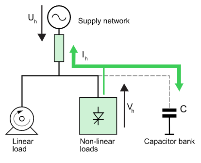
Resonance occurs when the denominator (1-LSCω2) tends toward zero. The corresponding frequency is called the resonance frequency of the circuit. At that frequency, impedance is at its maximum and high amounts of harmonic voltages appear because of the circulation of harmonic currents. This results in major voltage distortion. The voltage distortion is accompanied, in the LS+C circuit, by the flow of harmonic currents greater than those drawn by the loads, as illustrated on Figure M16.
The distribution network and the power factor correction capacitors are subjected to high harmonic currents and the resulting risk of overloads. To avoid resonance, antihamonic reactors can be installed in series with the capacitors.
Fig. M16 – Illustration of parallel resonance
Effects of harmonics – Increased losses
Losses in conductors
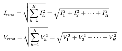
The active power transmitted to a load is a function of the fundamental component I1 of the current.
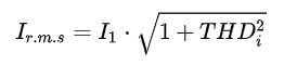
When the current drawn by the load contains harmonics, the rms value of the current, Ir.m.s, is greater than the fundamental I1
Fig. M17 – Reduced circulation of harmonic currents with detuned reactors
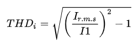
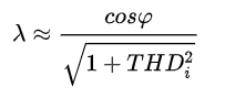
The definition of THDi being:
.
it may be deduced that :
.
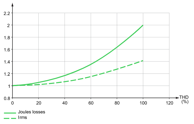
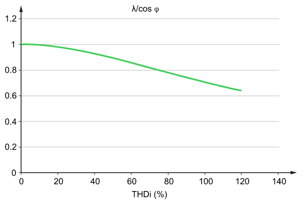
Figure M18 shows, as a function of the harmonic distortion:
• The increase in the r.m.s. current Ir.m.s. for a load drawing a given fundamental current • The increase in Joule losses, not taking into account the skin effect. (The reference point in the graph is 1 for Ir.m.s. and Joules losses, the case when there are no harmonics)
The harmonic currents cause an increase of the Joule losses in all conductors in which they flow and additional temperature rise in transformers, switchgear, cables, etc.
Fig. M18 – Increase in rms current and Joule losses as a function of the THD
Losses in asynchronous machines
The harmonic voltages (order h) supplied to asynchronous machines cause the flow of currents in the rotor with frequencies higher than 50 Hz that are the origin of additional losses.
Orders of magnitude
• A virtually rectangular supply voltage causes a 20% increase in losses • A supply voltage with harmonics u5 = 8% (of U1, the fundamental voltage), u7 = 5%, u11 = 3%, u13 = 1%, i.e. total harmonic distortion THDu equal to 10%, results in additional losses of 6%
Losses in transformers
Harmonic currents flowing in transformers cause an increase in the “copper” losses due to the Joule effect and increased “iron” losses due to eddy currents. The harmonic voltages are responsible for “iron” losses due to hysteresis.
It is generally considered that losses in windings increase as the square of the THDi and that core losses increase linearly with the THDu.
In Utility distribution transformers, where distortion levels are limited, losses increase between 10 and 15%.
Losses in capacitors
The harmonic voltages applied to capacitors cause the flow of currents proportional to the frequency of the harmonics. These currents cause additional losses.
i.e. total harmonic distortion THDu equal to 10%. The amperage of the current is multiplied by 1.19. Joule losses are multiplied by (1.19)2, i.e. 1.4.
Effects of harmonics – Overload of equipment
Generators
Generators supplying non-linear loads must be derated due to the additional losses caused by harmonic currents.
The level of derating is approximately 10% for a generator where the overall load is made up of 30% of non-linear loads. It is therefore necessary to oversize the generator, in order to supply the same active power to loads
Uninterruptible power systems (UPS)
The current drawn by computer systems has a very high crest factor. A UPS sized taking into account exclusively the r.m.s. current may not be capable of supplying the necessary peak current and may be overloaded.
Transformers
• The curve presented below (see Fig. M19) shows the typical derating required for a transformer supplying electronic loads
Fig. M19 – Derating required for a transformer supplying electronic loads
Example: If the transformer supplies an overall load comprising 40% of electronic loads, it must be derated by 40%.
• Standard UTE C15-112 provides a derating factor for transformers as a function of the harmonic currents.
.
Asynchronous machines
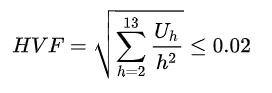
Standard IEC60034-1 (“Rotating electrical machines – Rating and performance “) defines a weighted harmonic factor (Harmonic voltage factor) for which the equation and maximum value are provided below.
.
Example
A supply voltage has a fundamental voltage U1 and harmonic voltages u3= 2% of U1, U5, = 3%, U7, = 1%. The THDu is 3.7% and the HVF is 0.018. The HVF value is very close to the maximum value above which the machine must be derated.
Practically speaking, asynchronous machines must be supplied with a voltage having a THDu not exceeding 10%.
Capacitors
According to IEC 60831-1 standard (“Shunt power capacitors of the self-healing type for a.c. systems having a rated voltage up to and including 1 000 V – Part 1: General – Performance, testing and rating – Safety requirements – Guide for installation”), the r.m.s. current flowing in the capacitors must not exceed 1.3 times the rated current.
Using the example mentioned above, the fundamental voltage U1, harmonic voltages u5 = 8% (of U1), U7 = 5%, U11 = 3%, U13, = 1%, i.e. total harmonic distortion THDu equal to 10%, the result is
Ir.m.s./I1 = 1.19, at the rated voltage. For a voltage equal to 1.1 times the rated voltage,the current limit
Ir.m.s./I1 = 1.3 is reached and it is necessary to resize the capacitors.
Neutral conductors
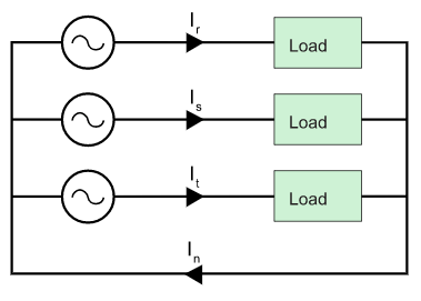
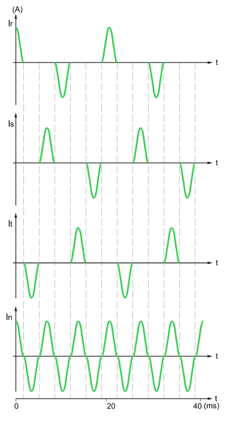
Consider a system made up of a balanced three-phase source and three identical single-phase loads connected between the phases and the neutral (see Fig. M20).
Fig. M20 – Flow of currents in the various conductors connected to a three-phase source
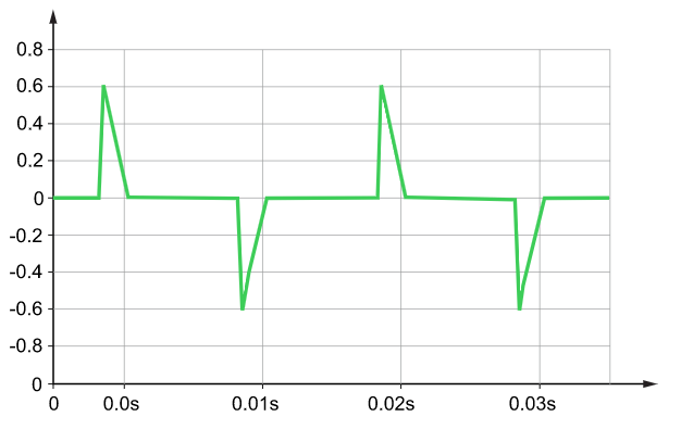
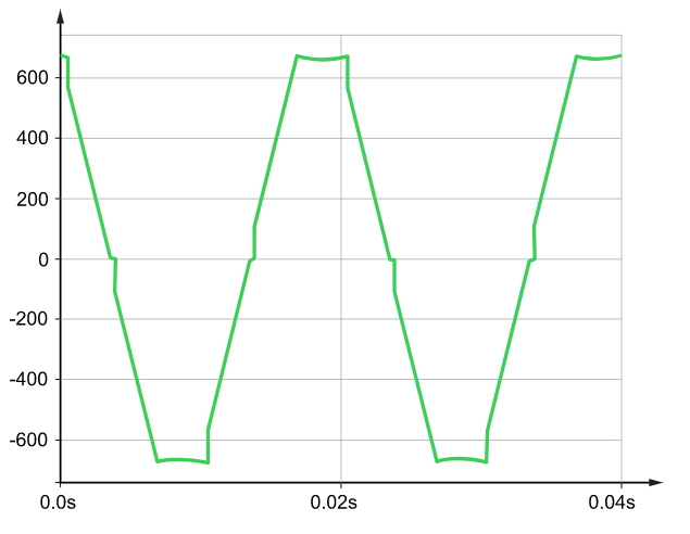
Figure M21 shows an example of the currents flowing in the three phases and the resulting current in the neutral conductor.
In this example, the current in the neutral conductor has a rms value that is higher than the rms value of the current in a phase by a factor equal to the square root of 3.
The neutral conductor must therefore be sized accordingly.
Fig. M21 – Example of the currents flowing in the various conductors connected to a three-phase load (In = Ir + Is + It)
The current in the neutral may therefore exceed the current in each phase in installation such as those with a large number of single-phase devices (IT equipment, fluorescent lighting). This is the case in office buildings, computer centers, Internet Data Centers, call centers, banks, shopping centers, retail lighting zones, etc.
This is not a general situation, due to the fact that power is being supplied simultaneously to linear and/or three-phase loads (heating, ventilation, incandescent lighting, etc.), which do not generate third order harmonic currents. However, particular care must be taken when dimensioning the cross-sectional areas of neutral conductors when designing new installations or when modifying them in the event of a change in the loads being supplied with power.
A simplified approach can be used to estimate the loading of the neutral conductor.
For balanced loads, the current in the neutral IN is very close to 3 times the 3rd harmonic current of the phase current (I3), i.e.: IN ≈ 3.I3
This can be expressed as: IN ≈ 3. i3 . I1
For low distortion factor values, the r.m.s. value of the current is similar to the r.m.s. value of the fundamental, therefore: IN ≈ 3 . i3 IL
And: IN /IL ≈ 3 . i3 (%)
This equation simply links the overloading of the neutral (IN /IL) to the third harmonic current ratio.
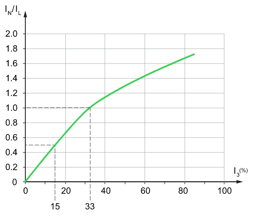
In particular, it shows that when this ratio reaches 33%, the current in the neutral conductor is equal to the current in the phases. Whatever the distortion value, it has been possible to use simulations to obtain a more precise law, which is illustrated in Figure M22
Fig. M22 – Loading of the neutral conductor based on the 3rd harmonic ratio
The third harmonic ratio has an impact on the current in the neutral and therefore on the capacity of all components in an installation:
• Distribution panels • Protection and distribution devices • Cables and trunking systems
According to the estimated third harmonic ratio, there are three possible scenarios: ratio below 15%, between 15 and 33% or above 33%.
Third harmonic ratio below 15% (i3 ≤ 15%):
The neutral conductor is considered not to be carrying current. The cross-sectional area of the phase conductors is determined solely by the current in the phases. The cross-sectional area of the neutral conductor may be smaller than the cross-sectional area of the phases if the cross sectional area is greater than 16 mm2 (copper) or 25 mm2 (aluminum).
Protection of the neutral is not obligatory, unless its cross-sectional area is smaller than that of the phases.
Third harmonic ratio between 15 and 33% (15 < i3 ≤ 33%), or in the absence of any information about harmonic ratios:
The neutral conductor is considered to be carrying current.
The operating current of the multi-pole trunking must be reduced by a factor of 0.84 (or, conversely, select trunking with an operating current equal to the current calculated, divided by 0.84).
The cross-sectional area of the neutral MUST be equal to the cross-sectional area of the phases.
Protection of the neutral is not necessary.
Third harmonic ratio greater than 33% (i3 > 33%)
This rare case represents a particularly high harmonic ratio, generating the circulation of a current in the neutral, which is greater than the current in the phases.
Precautions therefore have to be taken when dimensioning the neutral conductor.
Generally, the operating current of the phase conductors must be reduced by a factor of 0.84 (or, conversely, select trunking with an operating current equal to the current calculated, divided by 0.84). In addition, the operating current of the neutral conductor must be equal to 1.45 times the operating current of the phase conductors (i.e. 1.45/0.84 times the phase current calculated, therefore approximately 1.73 times the phase current calculated).
The recommended method is to use multi-pole trunking in which the cross-sectional area of the neutral is equal to the cross-sectional area of the phases. The current in the neutral conductor is therefore a key factor in determining the cross sectional area of the conductors. Protection of the neutral is not necessary, although it should be protected if there is any doubt in terms of the loading of the neutral conductor.
This approach is common in final distribution, where multi-pole cables have identical cross sectional areas for the phases and for neutral.
With busbar trunking systems, precise knowledge of the temperature rises caused by harmonic currents enables a less conservative approach to be adopted. The rating of a busbar trunking system can be selected directly as a function of the neutral current calculated.
Effects of harmonics – Disturbances affecting sensitive loads
Effects of distortion in the supply voltage
Distortion of the supply voltage can disturb the operation of sensitive devices:
• Regulation devices (temperature) • Computer hardware • Control and monitoring devices (protection relays)
Distortion of telephone signals
Harmonics cause disturbances in control circuits (low current levels). The level of distortion depends on the distance that the power and control cables run in parallel, the distance between the cables and the frequency of the harmonics.
Effects of harmonics – Economic impact
Energy losses
Harmonics cause additional losses (Joule effect) in conductors and equipment.
Higher subscription costs
The presence of harmonic currents can require a higher subscribed power level and consequently higher costs. What is more, Utilities will be increasingly inclined to charge customers for major sources of harmonics.
Oversizing of equipment
• Derating of power sources (generators, transformers and UPSs) means they must be oversized • Conductors must be sized taking into account the flow of harmonic currents. In addition, due the skin effect, the resistance of these conductors increases with frequency. To avoid excessive losses due to the Joule effect, it is necessary to oversize conductors • Flow of harmonics in the neutral conductor means that it must be oversized as well
Reduced service life of equipment
When the level of distortion THDu of the supply voltage reaches 10%, the duration of service life of equipment is significantly reduced. The reduction has been estimated at:
• 32.5% for single-phase machines • 18% for three-phase machines • 5% for transformers
To maintain the service lives corresponding to the rated load, equipment must be oversized.
Nuisance tripping and installation shutdown
Circuit-breakers in the installation are subjected to current peaks caused by harmonics. These current peaks may cause nuisance tripping of old technology units, with the resulting production losses, as well as the costs corresponding to the time required to start the installation up again.
Examples
Given the economic consequences for the installations mentioned below, it was necessary to install harmonic filters.
Computer centre for an insurance company In this centre, nuisance tripping of a circuit-breaker was calculated to have cost 100 k€ per hour of down time.
Pharmaceutical laboratory Harmonics caused the failure of a generator set and the interruption of a long duration test on a new medication. The consequences were a loss estimated at 17 M€.
Metallurgy factory A set of induction furnaces caused the overload and destruction of three transformers ranging from 1500 to 2500 kVA over a single year. The cost of the interruptions in production were estimated at 20 k€ per hour.
Factory producing garden furniture The failure of variable-speed drives resulted in production shutdowns estimated at 10 k€ per hour.
Published by Ahmad Ezzeddine, EE Power – Technical Articles: Power Factor Correction: Reactive Power Compensation Methods, December 15, 2022.
This article introduces power factor correction, why it is needed, and how to design it for the system.
Increasing photovoltaic penetration tied to the grid has caused many problems for utility providers. One of the main problems is that most of the power electronics used consume reactive power, which causes low power factor and system instability–a problem that has put power factor correction methods under development again. This article discusses the two most used reactive power compensation methods.
S2 (KVA) = P2 (KW) + Q2 (KVAR)
The relation between the power types.
Power Factor
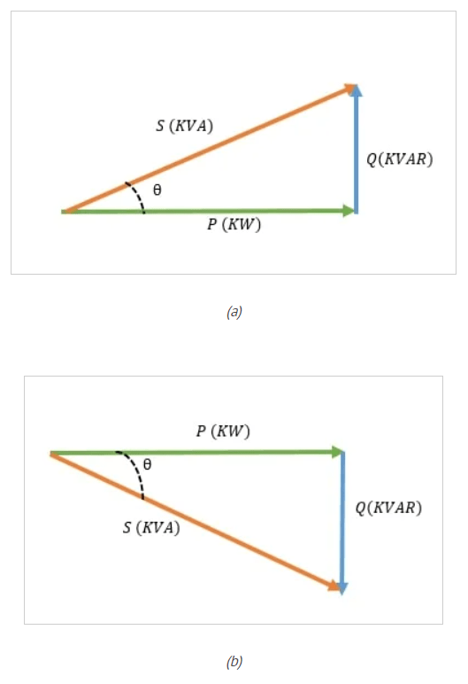
The electric power used to run an appliance is called demand power or apparent power expressed in Volt-Ampere (S). The apparent power is a combination of two powers, true power expressed in Watt (P) and reactive power expressed in VAR (Q).
Power factor determines the system’s power efficiency and is the ratio between true power and apparent power. The lower the power factor, the less efficient a power system is. The power factor lags with inductive load and leads with capacitive load. Resistive loads have a unity power factor.
Figure 1. (a)-the power factor expresses as cosθ leading power factor. (b)-lagging power factor. Image used courtesy of Ahmad Ezzeddine
Power Factor Correction
Power factor correction drives power factor to unity. The importance behind power factor correction lies within the effects of having a low power factor on energy prices, instrument lifetime, and accessory sizing, such as electrical cables.
Generally, induction machines used in industrial factories running at low loads, arc lamps, and varying power usages at short intervals cause a low lagging power factor. Therefore, utilities charge those factories using a power factor or maximum demand tariff (KVA tariff).
Machines, conductors, and electrical accessories running at low power factor will have overheating problems due to that lower lifetime. With all this in mind, utilities and consumers seek a way to ensure power factor is close to unity.
The principle of Power Factor Correction
All power factor improvement methods lay under the same principle. For every load with a lagging power factor, a load with a leading power factor must be connected in parallel to ensure a power factor close to unity.
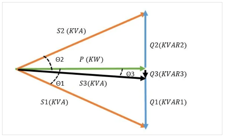
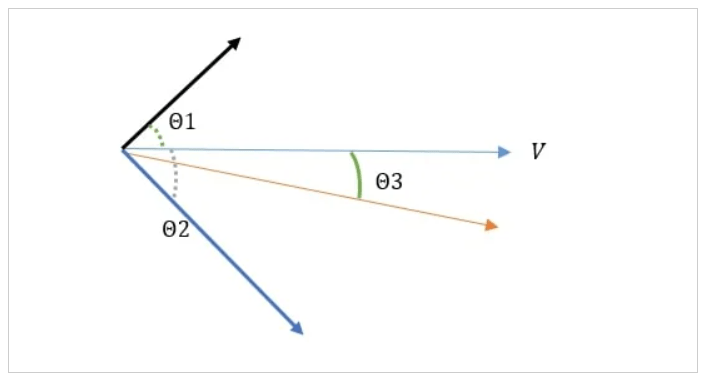
Figure 2. In this diagram, S1 is the power of a load Q1 is the lagging reactive power and cosθ1 is the power factor. Introducing a leading load with Q2 as reactive power causes the formation of S3, the power for the formed system, Q3 minimized lagging reactive power and cosθ3, an overall power factor after correction closer to a unity power factor at P. Image used courtesy of Ahmad Ezzeddine
The equation relating to the image above is
Q3 = Q1 – Q2 = P ∗ (tan(Θ1) – tan(Θ2))
Power Factor Correction Methods
There are several methods used for power factor correction. The 2 most used are capacitor banks and synchronous condensers.
1. Capacitor Banks:
• Capacitor banks are systems that contain several capacitors used to store energy and generate reactive power. Capacitor banks might be connected in a delta connection or a star(wye) connection.
• Power capacitors are rated by the amount of reactive power they can generate. The rating used for the power of capacitors is KVAR. Since the SI unit for a capacitor is farad, an equation is used to convert from the capacitance in farad to equivalent reactive power in KVAR.
In the equation below, C is the capacitance in microfarads, V is the voltage in volts, and f is the frequency in hertz
KVAR = C ∗ 2π ∗ f ∗ V2 ∗ 10-9
• Capacitor banks are designed to operate in stages. Since capacitors have a leading power factor, and reactive power is not a constant power, designing a capacitor bank must consider different reactive power needs. For example, the configuration for a 5-stage capacitor bank with a 170 KVAR maximum reactive power rating could be 1:1:1:1:1, meaning 5*34 KVAR or 1:2:2:4:8 with 1 as 10 KVAR. The stepping of stages and their number is set according to how much reactive power changes in a system.
• Capacitor bank systems have other elements, such as protection components: contactors and switch disconnectors, HRC fuses, and circuit breakers. Also, capacitor banks need an enclosure to protect them from overheating, dust, and water.
• Detuning reactors are connected to capacitor banks in series to deal with voltage and current distortions.
• Discharge resistors are also used for each capacitor to discharge it after being disconnected from the supply in a relatively short time interval.
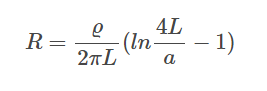
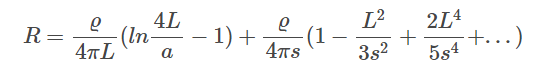
•To calculate the maximum discharge resistance, a ratio between the maximum discharge time approved by IEC60831 and a logarithmic capacitor charging must be applied.
Maximum Discharge Resistance = Maximum Discharge Time / (⅓ Capacitance * log (√2*Line Voltage / Capacitor Discharge Voltage))
• Capacitor banks not only create a stable system but cause lower KVAH consumption and have a good payback period even when neglecting maintenance and life costs of appliances running at low power factor.
Comparing two 60 kW systems running at 0.6 pf for 10 hours a day. The first system has no power factor improvement system, and the second has a capacitor bank connected in parallel with the appliances correcting the power factor to unity.
The yearly bill will be: total demand * operating hours * 365 * unit price
The total demand for the first system will be: (60(KW)/(0.6 pf))* 10 *365 * unit price per KVAH= 365000 unit price.
The total demand of the second system will be: 60*10*365 * unit price per KVAH= 219000 unit price.
The total improvement in the yearly bill will be: 365000-219000= 146000 unit price
Note: Interest rates, maintenance and operation costs, and other factors were ignored. The calculations above are used to simplify and show how power factor correction could change energy bills.
2. Synchronous Condensers:
• Synchronous condensers are simply over-excited synchronous motors running at no load. When connected in parallel with the loads, a synchronous condenser generates the needed reactive power for the system.
• The sizing of a synchronous condenser is proportional to the amount of reactive power that might be consumed by the electrical system.
• A synchronous motor runs at three different states. Underexited, intermediate excited, and overexcited. The states change with the change of excitation current. Under Excited synchronous motors act as an inductive load, therefore, consuming reactive power. Intermediate excited motors act as a resistive load, therefore, having no reactive power consumption or generation. Over-excited state, at this state current sine wave leads the voltage, therefore, generating reactive power at a leading power factor.
• In the phasor diagram below V is the voltage of the system and θ2 is the angle between the voltage and the load current. Cosθ2 is the lagging power factor showing that the system is consuming reactive power. A synchronous motor is added in parallel with the load and runs without loading the shaft.
Applying a large excitation current to the motor creates an over-excited state of the motor, therefore, producing cosθ1, a leading power factor. At this stage, the synchronous motor is generating reactive power and supplying it to the system
The resultant of the system is the vector summation of the load current and motor absorbed current, resulting in new current with an angle from system voltage θ3, cosθ3 is the resultant power factor of the system closer to a unity power factor.
Figure 3. Phasor diagram representing adding an overexcited synchronous condenser to a lagging load. Image used courtesy of Ahmad Ezzeddine
• Synchronous condensers use an automatic excitation controller to measure the power factor of the system and operate at the required state. For example, a synchronous condenser is connected in parallel with a load of 50 kVAR reactive power. The synchronous motor will be over-excited to reach a 50 KVAR reactive power generation. Another load operating at 37.5 KVAR is connected to the system, then the control unit of the synchronous condenser will increase its excitation current until it covers the extra 37.5 KVAR.
• To calculate the reactive power(Q) generated by a synchronous condenser, consider the internal machine voltage Ei and the terminal phase voltage Ep.
Q= 3Ep * (Ei – Ep) /Xd. Where Xd is the synchronous motor reactance.
• The advantage of synchronous condensers over capacitor banks is that they could generate the exact amount of reactive power needed. Whereas a capacitor bank will generate the total reactive power of the nearest stage to the load.
• With the recent huge penetration of renewable energy into the grid, power factor and voltage stability became a concern for utility operators. So, synchronous condensers are becoming the modern topic of research. A lot of research is ongoing regarding virtual synchronous machines. Moreover, new methods of implementing synchronous condensers to different positions on the grid are being studied.
Capacitor Banks vs. Synchronous Condensers
Capacitor banks and synchronous condensers might be used for similar applications. But, usually, capacitor banks are used in factories and low-capacity substations. Synchronous condensers are most feasible with high powers above 200 MVA stations and HVDC converter stations.
Table 1. Capacitor Banks vs. Synchronous Condensers
Author: Ahmad Ezzeddine is an electrical power and machines engineer with a degree from Beirut Arab University. Ahmad’s love for reading has developed his passion for writing about power electronics. In his free time, you can find Ahmad playing chess, reading, or hiking. Email: ahmadezzeddine@outlook.com
Published by Zbigniew ŁUKASIK1, Jacek KOZYRA1, Aldona KUŚMIŃSKA-FIJAŁKOWSKA1 Uniwersytet Technologiczno-Humanistyczny w Radomiu, Wydział Transportu i Elektrotechniki (1)
Abstract. A new method of established and justified level of operational costs for distribution network operators in a new model of regulation in force in the years 2016 – 2020 is described in this article. The changes made in 2016 are supposed to estimate operational costs of the enterprises distributing electricity to the costs taken into account in calculation of tariffs. A consequence of non-fulfilment of conditions and indexes in accordance with an idea of the new system is lowered value of return of capital and poor efficiency of enterprises in reduction of SAIDI indexes.
Streszczenie. Opracowanie przedstawia opis nowej metody ustalonego uzasadnionego poziomu kosztów operacyjnych dla Operatorów Systemów Dystrybucyjnych zawartej w nowym modelu regulacji obowiązującym na lata 2016 – 2020. Zmiany wprowadzone w 2016 roku mają doszacować koszty operacyjne przedsiębiorstw zajmujących się dystrybucją energii elektrycznej do kosztów uwzględnianych w kalkulacjach taryf na lata 2016- 2020. Konsekwencją niespełnienia warunków i wskaźników zgodnie z ideą nowego systemu jest obniżenie wartości zwrotu kapitału i słaba efektywność przedsiębiorstw w obniżaniu wskaźników dotyczących czasu trwania przerw w dostarczaniu energii elektrycznej. Monitorowanie pracy sieci średniego napięcia za pomocą wskaźników trwania przerw w dostarczaniu energii elektrycznej
Słowa kluczowe: Operator Systemu Dystrybucyjnego, Wskaźniki ciągłości dostaw energii, Wskaźniki operacyjne, Urząd Regulacji Energetyki, URE, OSD, SAIFI, SAIDI, CRP, WSD. Keywords: Distribution network operator (DNO), continuity of electricity supply rates, operational rates, Energy Regulatory Office, URE, DNO, SAIFI, SAIDI, CRP, WSD.
Introduction
European Union and Energy Regulatory Office sets the following goals for the companies from electrical power sector: continuity of electricity supply, an increase in reliability and the use of renewable sources of energy. These requirements are related to electrical power security of the states, in terms of operation and maintenance of power lines [1], [2].
Therefore, electrical power infrastructure requires larger number of inspections, repairs or complete modernization [18]. Therefore, the solutions supporting an analysis of failure frequency are required, as well as solutions that will improve switching of damaged fragments of the lines.
Distribution network operators are more and more involved in accomplishment of above goals, which results in higher quality of supplied energy.[3], [4], [14].
The basic goal of the publication is to compare SAIDI indexes and to present a new method of established and justified level of operational costs for distribution network operators.
The main causes of failures in medium-voltage lines
Medium-voltage transmission lines in Poland consist in 80% of overhead lines and in 20% of cable lines. The number of cable lines is increasing every year due to modernization and changing overhead lines into cable lines. The majority of medium-voltage lines were built in the 1970s-1980s. AFL-6 cables from 25 mm2 in diameter on the branches of lines up to 70 mm2 at the stem of low voltage line were usually used for the construction of overhead lines.
Due to increased power demand from the customers, diameters of the lines, particularly on the branches can be insufficient. These structures were supported by poles: ŻN (reinforced concrete), BSW (prestressed concrete), ŻW (reinforced concrete high). These rods were between 10 and 14 m high and between 1,1 and 4,4 kN of tension. The poles were equipped with supporting insulators (linear standing rod) and linear hanging rod insulators [5]. The disadvantage of overhead lines is their sensitivity to external and atmospheric factors. The birds, branches and natural process of ageing have big impact on failure frequency of overhead lines.[17] The examples of damages resulted from ageing and branches are presented on Fig. 1.
Fig.1. The examples of damages to overhead lines: the ageing of the structure [15], and damages caused by branches of trees [16]
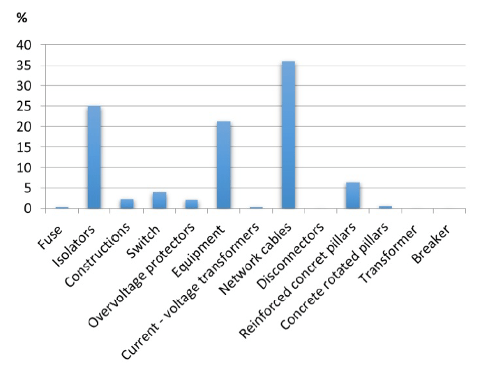
Fig.2. The percentage share of damages of particular elements of low voltage lines
The wires, insulators and poles made of reinforced concrete are the parts that are usually damaged. The percentage share of these elements in damaged lines in total is presented on Fig.2. The majority of damages is caused by the time that elements of medium-voltage lines are used. The structures and drives of switchgears corrode and break down with time.
Another cause of failure, not resulting directly from the age of a line, is insufficient number of cutting of trees and branches close to the lines. It is often caused by formal and legal problems with the access to real estate. The falling of a tree or branches on the line can damage wires, pole structure and even the very poles.
Above deliberations are confirmed by an analysis of SAIDI (System Average Interruption Duration Index) in 2015 for three selected departments from central Poland. The longest interruptions in electricity supply were caused by material ageing, and then by trees and branches and atmospheric discharges. SAIDI indexes divided into causes of failures for three departments are presented on Fig.3.
Fig.3. SAIDI indexes unplanned with catastrophic ones divided into causes of failures for three selected departments [6]
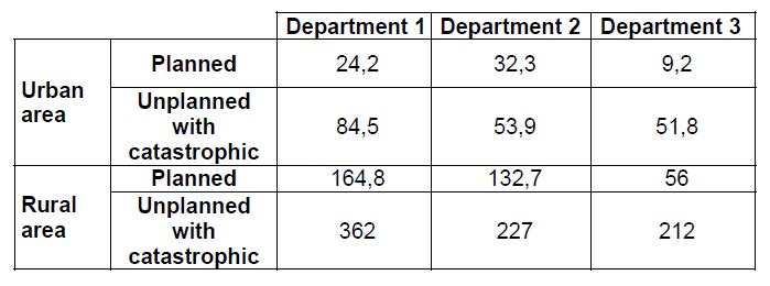
SAIDI indexes in urban and rural areas are presented in table 1. About 80% of failures occur in rural areas. It is probably caused by the fact that majority of low voltage lines in urban areas is cabled, which limits occurrence of such failure frequency factors as „trees and branches”, „gales”, „birds and animals”.
Table 1. SAIDI indexes planned and unplanned with catastrophic ones divided into rural and urban areas for three selected departments [6]
.
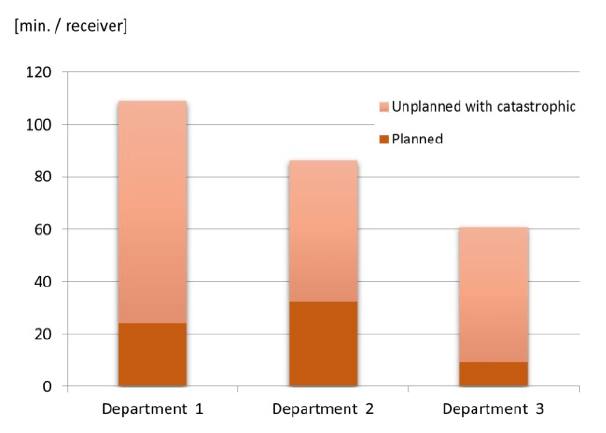
Apart from limiting the impact of external factors on medium-voltage lines in urban area, the high impact on reaction to failures and restoration of power has ring work system and an option of quick disconnection of damage fragment of a line. Switching is made with the use of radio-controlled switch disconnectors placed in a few places of medium-voltage lines. They enable to section off even the smallest fragment of a failed line. The location of radio-controlled switch disconnectors is also important. They are supposed to reduce the number of transformer stations without power supply during failure. 3 departments in terms of their SAIDI index in an urban area were compared on Fig. 4 and in rural areas on Fig. 5.
Fig.4. SAIDI indexes planned and unplanned with catastrophic ones in urban area for three selected departments [6]
Fig.5. SAIDI indexes planned and unplanned with catastrophic ones in rural area for three selected departments [6]
The comparison of indexes monitoring medium-voltage failure frequency
An order of the Minister of Economy on the conditions of functioning of electrical power system imposes an obligation to reveal SAIDI indexes on distribution network operators [7]. Publishing data is an assessment of efficiency of enterprises and it is supposed to increase quality of services of distribution of electricity, maintaining price affordability of these services, and current level of investments.
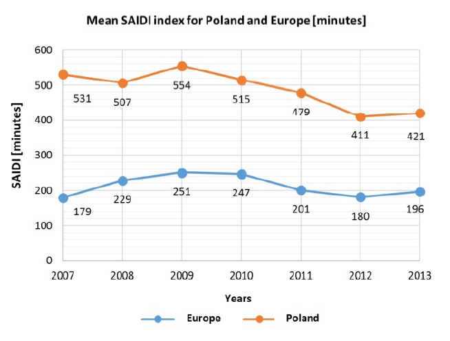
Fig.6. Mean SAIDI index calculated as the sum of planned and unplanned interruptions, including interruptions caused by disasters, for selected countries of Europe, and Poland from 2007 – 2013 [8], [9]
The level of capital expenditures of 4 largest electrical power DNOs has considerably increased in recent years. It is estimated that this level increased in the years 2009-2014 by over 50% [8]. Despite these investments, the level SAIDI and SAIFI (System Alergen Interruption Frequency Index) indexes in Poland still differ from European average. The comparison of average SAIDI and SAIFI indexes in the years 2007-2014 in Poland and selected European countries is presented on Fig.6 and Fig.7.
Fig.7. Mean SAIFI index calculated as the sum of planned and unplanned interruptions, including interruptions caused by disasters, for selected countries of Europe, and Poland from 2007 – 2013 [8], [9].
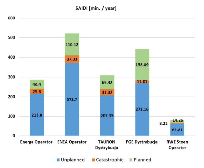
SAIDI and SAIFI indexes for the largest five distribution network operators in 2015 are presented on Fig.8 and Fig.9.
Fig.8. SAIDI index divided into type of interruptions for the largest five distribution network operators in 2015
Fig.9. SAIFI index divided into type of interruptions for the largest five distribution network operators in 2015
Due to big differences between Poland and other European countries and due to necessity to improve the quality of services provided by the Operators, the director of Energy Regulatory Office decided to introduce a new model of regulation for the years 2016 – 2020. The improvement of quality of services of distribution of electricity provided for customers should be the main goal. The works on implementation of a new regulation began in 2014. The director of Energy Regulatory Office obliged five largest DNOs to install balancing meters in medium and low voltage stations. The number of installed meters is supposed to correspond to specific representative group of customers at the end of 2015, that is, about 51% of customers and minimum 80% of customers in 2018. It will enable to determine, among others, duration of interruptions in electricity supply on low voltage side [10]. Looking ahead, it will be possible to measure on its basis, among others, the duration of supply interruptions on low voltage side and, as a result, to take appropriate actions by DNO to increase the quality of services of distribution of electricity provided to customers.
The emphasis will be put on the improvement of quality of services of distribution of electricity provided to customers, and the indexes having direct impact on income of DNO will be SAIDI and SAIFI indexes, adjusted for the purposes of qualitative regulation and index illustrating Connection Realization Time (CPR) of 4th and 5th energy consumer group. In 2018, Transmission of Metering and Billing Data Time (CPD) read from data interchange system in ebIX standard will be added to a new model of regulation.
The rules of calculating regulated income in a new model in a enterprise dealing with distribution of electricity are determined with the use of following dependency [8]:
(1) PR = Ko+ A + PS + Kzk + KRB + Te+ Kp + P
where: PR – regulated income, Ko – operating costs, A – amortization, PS – power grid assets tax, Kzk – the costs of capital employed, KRB – the costs of balance difference, Te – the costs of transit of energy, Kp – the costs of purchase of transmission services to OSP, P – remaining elements of regulated income.
In a model in force in the years 2011 – 2015, the value of return on capital employed in a tariff for a given year was determined by dependency (2):
(2) Kzk = WRAt * WACCt
where: Kzk – return on capital employed in a tariff in t year, WRAt – regulating asset value for t year (with AMI investments), WACCt – weighted average cost of capital established for t year (increased by 7% for AMI investments).
The method of calculating return on capital employed has changed in a model, which will be in force in the years 2016 – 2020. A dependency (3) describing the method of calculating the costs of capital employed is presented below:
(3) Kzk = WRAt * WACCt * Qt * WRt
where: Kzk– return on capital employed in a tariff in t year, WRAt– regulating asset value for t year (with AMI investments arranged with the director of URE until March 31, 2015), WACCt – weighted average cost of capital established for t year (increased by AMI investments arranged with the director of URE until March 31, 2015 o 7%), Qt – qualitative regulation coefficient, WRt– regulating rate.
Two new coefficients were introduced in comparison with previous model:
– qualitative regulation coefficient Qtbetween 0,85÷1,0 taking lack of appropriate effects of qualitative regulation into account,
– regulating rate WRt (determined individually for each DNO) between 0,9 ÷ 1,1 taking assessment of innovative character of actions taken by DNO into account.
Operational costs of distribution network operators
One of the main factors accepted in a new model of calculating regulated income is a rate of operational costs. Between 2008 and 2014, distribution network operators had higher costs than were taken into account in calculation of tariffs for the analysed period. These costs were higher in the years 2008 – 2014 by 20,7% and by 7,8% in the years 2012 – 2014. In 2014, only three operators had lower costs [11]. Taking actions of DNOs within the scope of efficiency improvement into account, efficiency improvement was checked by determining arithmetic mean of operational costs analysed in the years 2008 – 2014 in prices for the year 2015 for each DNO. Calculated mean value was reduced by the costs of assumed efficiency improvement. The costs assumed for the year 2020 do not take only efficiency improvement of DNOs into account, but also forecasted action scale growth of operators.
Taking energetic interests of enterprises and customers into consideration, the costs resulting from a new model for the years 2016 -2020 with the costs taken into account in calculation of tariffs in 2015 were combined. Assuming the costs expressed in permanent prices in 2015, the following formula (4) can be applied to determine the costs for a given year of regulation period 2016 – 2020:
.
where: Ktax t– the costs to be taken into account in calculation of tariffs, t – another year of tariff t (2016, 2017, 2018, 2019, 2020), Ktax 2015 – model costs taken into account in calculation of tariff of an enterprise for the year 2015, Kmodel 2020 – model costs in 2020 (in prices from 2015), resulting from a new model of assessment of operational costs, taking efficiency improvement and action scale growth of the enterprises into consideration.
Above formula was in effect until 2016, whereas the dependency defined in §21.1 of the publication [12] should be used to determine tariff costs in the years 2017 – 2020:
(5) Kwn≤Kwn-1· [1 + (RPI – Xn) / 100]
where: Kwn, Kwn-1 – prime costs of an energy enterprise related to business activity, taking conditions of such business activity into consideration, Xn – correction coefficients defining efficiency improvement of an energy enterprise, determined for particular years in a year of extending the tariff for confirmation [%], RPI – annual average rate of prices of consumer goods and services in total, in a calendar year preceding a year of working out a tariff [%].
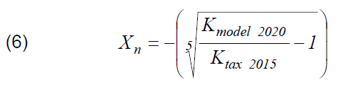
The value of correction coefficients Xn for the years 2017-2020 is determined from the dependency (6) which is enabled by application of a new method of establishing justified level of operational costs:
.
To apply a new method of established and justified level of operational costs, it is required to calculate the level of effective costs in the years 2008-2014. The following dependency is applied for this purpose (7)
(7) KEt = KBt· (1 – PEKI) · (1 – PEKS)
where: KEt– the level of effective costs in t year, KBt – base costs of t year, PEKI – individual efficiency improvement coefficient between 2016 and 2020, PEKS – sector efficiency improvement coefficient between 2016 and 2020.
A base cost is an operational cost of distribution, that is, distribution costs excluding amortization, the costs of energy purchase to cover balance sheet difference, the costs of purchase of distribution and transmission services, the costs of power grid assets tax and concession fees. A base cost is reduced by the costs of:
– the fees for perpetual usufruct of land in the field of power grid assets, – the fees for permanent land exemption from an agricultural use, – the fees for transmission easement for state-owned forests, – the fees for placing devices of technical infrastructure or buildings on a roadway, – the costs of workers’ tariff, – the costs resulting from changing the state of actuarial reserves on account of workers’ tariff, – the costs resulting from the change in actuarial reserves on other accounts, – one-off costs of Voluntary Redundancy Programs and other one-off costs.
The value of model costs in the years 2008-2014, Kmodel 2008 -2014, was calculated as arithmetic mean of discounted effective costs (from the years 2008-2014) for the year 2015.
It was also necessary to check the impact of mean DNO action scale growth on the costs of enterprises in the years 2016-2020 and potential new obligations of DNO by applying action scale growth coefficient (WSD).
Model costs in 2020, Kmodel 2020, taking efficiency improvement and DNO action scale growth into account, was calculated in accordance with the following formula (8):
(8) Kmodel 2020 = Kmodel 2008 -2014· (1 + WSD)
where: Kmodel 2020 – model costs in 2020, resulting from a new model of assessment of operational costs, taking efficiency improvement and action scale growth of the enterprises into consideration, WSD – action scale growth rate.
The application of a new method of established and justified level of operational costs requires the knowledge of base costs of DNO in the years 2008-2014 and the value of sector efficiency improvement coefficient in the years 2016- 2020, which was determined at the level of PEKS = 10%. An individual efficiency improvement coefficient between 2016 and 2020 for all DNOs was assumed as PEKI = 0 [13]. The value of action scale growth rate in the years 2016-2020, WSD = 2,5%.
Conclusions
With reference to low voltage energy infrastructure, the major cause of failures is old devices, trees, atmospheric phenomena. The distribution network operators systematically try to modernize lines to improve the first cause. However, this process requires time and financial outlays. The second cause of failures is eliminated by DNOs by cutting trees in the vicinity of power lines. However, it is sometimes not possible, because the access to real estate is often difficult for formal and legal reasons. DNOs can’t do too much to eliminate the third cause. Therefore, the goal is to limited the time of failure and number of medium-voltage lines and transformer stations left without power supply during removal of failure. SAIFI and SAIDI indexes are good determinants of effectiveness of these actions.
The list of SAIDI and SAIFI indexes for five distribution network operators in the years 2011-2015 is presented in the thesis. The situation is improving every year. Based on attached charts, we can see the emphasis that DNOs put on reduction of these indexes.
It is necessary to implement a new model of regulation to increase quality of services provided by distribution network operators. The implementation of qualitative regulation is both chance and challenge for distribution companies. It gives operators an opportunity to improve their image and increase efficiency of enterprises. Another benefit from implementation of a new regulation DNO, taking the state of power grids into account, will be a plan of network investments, new sources of energy, showing the areas recommended to modernization and rebuilding.
REFERENCES
[1] Kozyra J.: Monitorowanie i diagnozowanie uszkodzeń w procesach wytwarzania i przesyłu energii elektrycznej. Logistyka, 3/2015 [2] Kuśmińska-Fijałkowska A., Łukasik Z.: Efekty wynikające z wdrożenia Systemu Zarządzania Jakością. Logistka 3/2014 [3] Kuśmińska-Fijałkowska A., Łukasik Z.: Koordynowanie działań w organizacji w odniesieniu do Systemu Zarządzania Jakością. Logistka 3/2014 [4] Kozyra J., Warchoł R.: Wykorzystanie energoelektronicznych systemów zasilania gwarantowanego AC w elektroenergetyce. Logistyka 6/2014 [5] Elprojekt Sp. z o.o., Album linii napowietrznych średniego napięcia 15-20 kV, Poznań 2011 [6] Opracowanie na podstawie statystyk OSD [7] Rozporządzenie Ministra Gospodarki z dnia 4 maja 2007 Dz.U. Nr 93, poz. 623 [8] Putynkowski G., Balawender P., Woźny K., Kozyra J., Łukasik Z., Kuśmińska-Fijałkowska A., Ciesielka E.: A New Model for the Regulation of Distribution System Operators with Quality Elements that Include the SAIDI/SAIFI/CRP/CPD Indices. Electrical Power Quality and Utilisation, Journal Vol. XIX, No. 1, 2016, ISSN: 1896-4672 [9] CEER Benchmarking Report 5.2 on the Continuity of Electricity Supply. Data update, Council of European Energy Regulators, Brussels 2015. [10] Strategia Regulacji Operatorów Systemów Dystrybucyjnych na lata 2016-2020 (którzy dokonali z dniem 1 lipca 2007 r. rozdzielenia działalności), Urząd Regulacji Energetyki Warszawa 2015 r. [11] Koszty operacyjne dla Operatorów Systemów Dystrybucyjnych na lata 2016-2020 (którzy dokonali z dniem 1 lipca 2007 r. rozdzielenia działalności) Urząd Regulacji Energetyki Warszawa 2015 r. [12] Rozporządzenie Ministra Gospodarki z dnia 18 sierpnia 2011r. w sprawie zasad kształtowania i kalkulacji taryf oraz rozliczeń w obrocie energią elektryczną. (Dz.U. z 2013 r. poz.1200) [13] Osiewalski J., Makieła K.: Koncepcja ustalania wybranych elementów kształtujących Przychód Regulowany OSD, którzy dokonali z dniem 1 lipca 2007r. rozdzielenia działalności – model kosztów operacyjnych i różnicy bilansowej, Kraków 2015. [14] Szmurło R., Starzyński J., Chaber B., Wincenciak S.: Flexible Scenarios Based System for Scientific Computing. Przegląd Elektrotechniczny Tom 88 nr. 4a, pp.117-119. (2012) [15] http://www.operator.enea.pl [16] http://wm.pl/ [17]Krysiuk, C., J. Brdulak, B. Zakrzewski. Bezpieczna infrastruktura w transporcie drogowym. Logistyka 4 (2014). [18]Wójcik W.: Modern Power Engineering.1, Monografia, s.197 Politechnika
Autorzy: prof. dr hab. inż. Zbigniew Łukasik, Uniwersytet Technologiczno-Humanistyczny, Wydział Transportu i Elektrotechniki, ul. Malczewskiego 29, 26-600 Radom, E-mail: z.lukasik@uthrad.pl; dr inż. Jacek Kozyra, Uniwersytet Technologiczno-Humanistyczny, Wydział Transportu i Elektrotechniki, ul. Malczewskiego 29, 26-600 Radom, E-mail:. j.kozyra@uthrad.pl; dr inż. Aldona Kuśmińska-Fijałkowska, Uniwersytet Technologiczno-Humanistyczny, Wydział Transportu i Elektrotechniki, ul. Malczewskiego 29, 26-600 Radom, E-mail:. a.kusmińska@uthrad.pl.
Source & Publisher Item Identifier: PRZEGLĄD ELEKTROTECHNICZNY, ISSN 0033-2097, R. 93 NR 9/2017. doi:10.15199/48.2017.09.30
Published by Electrical Installation Wiki, Chapter M. Power harmonics management – Harmonic measurement in electrical networks
Procedures for harmonic measurement
Harmonic measurements are carried out on industrial or commercial sites:
• Preventively, to obtain an overall idea on distribution-network status (network mapping), • In view of corrective action, to determine the origin of a disturbance and determine the solutions required to eliminate it, • To check the validity of a solution (following modifications in the distribution network to check the reduction of harmonic disturbances)
The harmonic indicators can be measured:
• By an expert present on the site for a limited period of time (one day), giving precise, but limited perception, • By instrumentation devices installed and operating for a significant period of time (at least one week) giving a reliable overview of the situation, • Or by devices permanently installed in the distribution network, allowing a follow-up of Power Quality.
One-shot or corrective actions
This kind of action is carried-out in case of observed disturbances, for which harmonics are suspected. In order to determine the origin of the disturbances, measurements of current and voltage are performed:
• At the supply source level, • On the busbars of the main distribution switchboard (or on the MV busbars), • On each outgoing circuit in the main distribution switchboard (or on the MV busbars).
For accurate results, it is necessary to know the precise operating conditions of the installation and particularly the status of the capacitor banks (operating or not, number of connected steps).
The results of measurement will help the analysis in order to:
• Determine any necessary derating of equipment in the installation, or • Quantify any necessary harmonic protection and filtering systems to be installed in the distribution network, or • Check the compliance of the electrical installation with the applicable standards or Utility regulations (maximum permissible harmonic emission).
Long-term or preventive actions
For a number of reasons, the installation of permanent measurement devices in the distribution network is very valuable.
The presence of an expert on site is limited in time and it is not always possible to observe all the possible situations. Only a number of measurements at different points in the installation and over a sufficiently long period (one week to a month) provide an overall view of operation and take into account all the situations that can occur following:
• Fluctuations in the supply source, • Variations in the operation of the installation, • The addition of new equipment in the installation.
Measurement devices installed in the distribution network prepare and facilitate the diagnosis of the experts, thus reducing the number and duration of their visits.
Permanent measurement devices detect any new disturbances arising following the installation of new equipment, the implementation of new operating modes or fluctuations in the supply network.
For an overall evaluation of network status (preventive analysis), this avoids:
• Renting of measurement equipment, • Calling in experts, • Having to connect and disconnect the measurement equipment. For the overall evaluation of network status, the analysis on the main low-voltage distribution switchboards (MLVS) can often be carried out by the incoming device and/or the measurement devices equipping each outgoing circuit,
For corrective actions, it is possible to:
• Determine the operating conditions at the time of the incident, • Draw-up a map of the distribution network and evaluate the implemented solution.
The diagnosis may be improved by the use of additional dedicated equipment in case of specific problem.
Harmonic measurement devices
Measurement devices provide instantaneous and average information concerning harmonics. Instantaneous values are used for analysis of disturbances linked to harmonics. Average values are used for Power Quality assessment.
The most recent measurement devices are designed referring to IEC standard 61000-4-7: “Electromagnetic compatibility (EMC) – Part 4-7: Testing and measurement techniques – General guide on harmonics and interharmonics measurements and instrumentation, for power supply systems and equipment connected thereto”.
The supplied values include:
• The harmonic spectrum of currents and voltages (amplitudes and percentage of the fundamental), • The THD for current and voltage, • For specific analysis: the phase angle between harmonic voltage and current of the same order and the phase of the harmonics with respect to a common reference (e.g. the fundamental voltage).
Average values are indicators of the long-term Power Quality. Typical and relevant statistical data are for example measures averaged by periods of 10 minutes, during observation periods of 1 week.
In order to meet the Power Quality objectives, 95% of the measured values should be less than specified values.
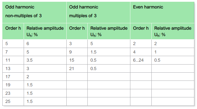
Fig. M10 gives the maximum harmonic voltage in order to meet the requirements of standard EN50160: “Voltage characteristics of electricity supplied by public distribution networks”, for Low and Medium Voltage.
Fig. M10 – Values of individual harmonic voltages at the supply terminals for orders up to 25 given in percent of the fundamental voltage U1
Portable instruments
The traditional observation and measurement methods include:
Oscilloscope
An initial indication on the distortion affecting a signal can be obtained by viewing the current or the voltage on an oscilloscope.
The waveform, when it diverges from a sinusoidal, clearly indicates the presence of harmonics. Current and voltage peaks can be observed.
Note, however, that this method does not offer precise quantification of the harmonic components.
Digital analyser
Only recent digital analysers can determine the values of all the mentioned indicators with sufficient accuracy.
They are using digital technology, specifically a high performance algorithm called Fast Fourier Transform (FFT). Current or voltage signals are digitized and the algorithm is applied on data relative to time windows of 10 (50Hz systems) or 12 periods (for 60Hz systems) of the power frequency.
The amplitude and phase of harmonics up to the 40th or 50th order are calculated, depending on the class of measurement.
Processing of the successive values calculated using the FFT (smoothing, classification, statistics) can be carried out by the measurement device or by external software.
Functions of digital analysers
• Calculate the values of the harmonic indicators (power factor, crest factor, individual harmonic amplitude, THD) • In multi-channel analysers, supply virtually in real time the simultaneous spectral decomposition of the currents and voltages • Carry out various complementary functions (corrections, statistical detection, measurement management, display, communication, etc.) • Storage of data
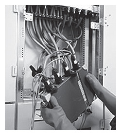
Fig. M11 – Implementation of a digital Power Quality recorder in a cabinet
Fixed instruments
Panel instrumentation provides continuous information to the Manager of the electrical installation. Data can be accessible through dedicated power monitoring devices or through the digital trip units of circuit breakers.
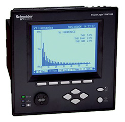
Fig. M12 – Example of Power and Energy meter
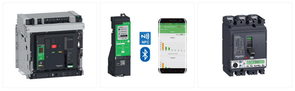
Fig. M13 – Example of electronic trip units of circuit-breakers providing harmonic related information
Which harmonic orders must be monitored and mitigated?
The most significant harmonic orders in three-phase distribution networks are the odd orders (3, 5, 7, 9, 11, 13 ….)
Triplen harmonics (order multiple of 3) are present only in three-phase, four-wire systems, when single phase loads are connected between phase and neutral.
Utilities are mainly focusing on low harmonic orders (5, 7, 11, and 13).
Generally speaking, harmonic conditioning of the lowest orders (up to 13) is sufficient. More comprehensive conditioning takes into account harmonic orders up to 25.
Harmonic amplitudes normally decrease as the frequency increases. Sufficiently accurate measurements are obtained by measuring harmonics up to order 30.
Published by Roland Buerger (Senseleq B.V.), Dr. Thomas Heid (CONDIS SA)
Internationally, it is not easy to specify the range of high voltage exactly. The boundary between medium and high voltage is between 30 kV and 100 kV, depending on local and historical conditions. In the current version of EN 50160 from 2020, the voltage levels are defined as follows.
Medium voltage: voltage, whose nominal RMS value is 1 kV < Un ≤ 36 kV High voltage: voltage, whose nominal RMS value is 36 kV < Un ≤ 150 kV
Voltage levels above 150 kV are thus assigned to extra-high voltage. The connection of generation plants such as large wind farms, conventional power plants, industrial parks and some large electricity consumers such as aluminum smelters are connected directly to the high or extra-high voltage grid. Accordingly, billing measurement often takes place here as well. In many countries, there are precise regulations regarding which technologies must be used for an official clearing measurement between two contracting parties.
Legal boundary conditions for billing measurement in Germany
In Germany, inductive current transformers are generally provided for current measurement, which must have an output signal of 1 or 5 A.1 For voltage measurement, inductive voltage transformers and capacitive voltage transformers have to be used.2 The capacitive voltage transformer consists of a capacitive divider, the high-voltage capacitor C1 and the intermediate voltage capacitor C2. A medium voltage transformer is in parallel with C2 and in series with a choke coil.
Figure 1: Capacitive voltage transformer
The compensation reactor is dimensioned so that the inductance is in resonance with the capacitance of the divider. The permissible output signals for voltage transformers are regulated in the PTB test rules for instrument transformers and are as follows:
100 V; 110 V; 100/√3 V; 110/√3 V; 2 x 100/√3 V; 2 x 110/√3 V; 200/√3 V; 220/√3 V und 2 x 200/√3 V
Free choice of measuring equipment from Um = 123 kV
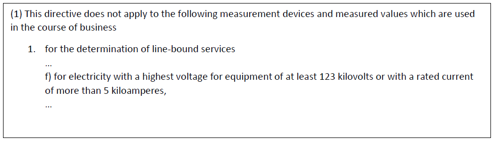
In the current Measuring and Calibration Directive (MessEV)3, an important note can be found on page 8 of 76 under § 5 with the heading “Uses excluded from the scope of application”.
Figure 2: Excerpt from the current German Measuring and Calibration Directive (MessEV)
The highest voltage for equipment is designated Um in IEC 61869-1 and is labeled with Um in IEC 61869-1 and is found on every rating plate of a voltage transformer as the first value in the rated insulation level of the primary connections for instrument transformers.
Figure 3: Example of a rating plate of a 110 kV voltage transformer
In this case, the nominal line voltage is 110 kV and correlates with the highest voltage for equipment (Um) 123 kV according to IEC 60038. Thus, in this example, the measuring equipment can be freely selected between the contracting parties in accordance with the MessEV. The reason for this procedure on the part of the authorities is that in the range above 123 kV or 5 kA nominal current, the qualification of the contracting parties is sufficient in any case to realize a professional billing measurement. In the voltage levels below that, the Measurement and Verification Ordinance can be interpreted as consumer protection. The directive ensures that the defined minimum standard is met without the contract partners having to negotiate the boundary conditions.
Actual instrument transformer status in high and extra-high voltage networks
Despite this flexibility of the contracting parties, inductive voltage transformers have been installed in the majority of cases for billing measurements in the ENTSO-E4 area. Defects in these devices usually lead to a total breakdown, so that inaccuracies in the measurement over a longer period of time are unlikely. Capacitive voltage transformers are avoided for this reason, as individual capacitors can be broken down without affecting operational safety. Amplitude and phase errors can deteriorate without being noticed, so that the specified accuracy class is no longer met. This scenario may well result in a major financial loss for a contracting party over a longer period of time. A special technical feature of the capacitive voltage transformer is that the device is operated in resonance at nominal frequency. The bandwidth of these capacitive high-voltage transformers can therefore be classified as very low. In 2012, an article was already published in the etz5 regarding the frequency behavior of transformers. In addition to inductive voltage transformers, a capacitive high-voltage voltage transformer was also measured.
Figure 4: Frequency response of a capacitive high voltage transformer
Already at approx. 450 Hz, a harmonic amplitude could be amplified by a factor of 2.2 (see Figure 4). Amplitude errors of approx. -75 % have also been measured below 1000 Hz in other devices.6
For inductive voltage transformers, an overview has been prepared by the international technical-scientific organization Cigré, which defines the usable range of inductive voltage transformers in general.
Table 1: Suitability of inductive transformers for harmonic measurements
(Source: CIGRE / CIRED Guidelines for Power Quality Monitoring WG C4.112 TECHNICAL BROCHURE 596)
Certainly not all designs available on the market have been tested, so outliers in both the positive and negative direction must be expected. Many end users believe that there is a strong attenuation of the higher-frequency components after the permitted bandwidth. This assumption often does not correspond to reality. The primary coil basically forms resonance points which can strongly attenuate but also amplify the primary signal transformed to the secondary side. Amplitude errors of 200 to 400 % are possible here.7 The resonance points can also be combined with phase errors greater than 90 °.
Figure 5: Frequency response of a 10 kV voltage transformer (12/28/75 kV) with a resonance point at approx. 6 kHz
In general, for inductive voltage transformers, the higher the voltage level, the closer the first resonance point is to the nominal frequency. For this reason, a measurement of harmonics in the extra-high voltage network from the 2nd to the 7th is no longer assured.
Digital energy meters and voltage transformers
While problems are primarily seen here in the measurement of voltage quality, problems also arise for billing measurement. This is because current energy meters in many cases have a larger analog bandwidth than the voltage transformer. This means that harmonics beyond the nominal frequency are passed on to the meter, sometimes significantly distorted. For example, the capacitive VT in Figure 4 amplifies an amplitude of 5% of the nominal voltage at 350 Hz by a factor of 1.6 and shifts its phase by about -20°. The distorted signal in blue is shown in the following diagram.
Figure 6: Primary signal with an amplitude of 5 % at 350 Hz without (red) and with distortion according to frequency response from Figure 4
The voltage signal is then digitized in the meter at an appropriate sampling rate. Existing energy meters such as the LZQJ-XC have a sampling rate of 3.2 kHz. Statements regarding the analog bandwidth are unfortunately not found in the data sheet.8 Thus, it can be assumed that amplitudes at even higher frequencies are basically included in the active power calculation.
Power of a wind turbine
According to the international standard for wind turbines IEC 61400-219, the wind turbine is allowed a THDV and a THDI of maximum 5% up to 2.5 kHz. This means that a wind turbine specified with 5 MW only must have an active power of 4.5125 MW at nominal frequency.
(0.95×𝑉) × (0.95×𝐼) = 0.9025 × 𝑃 = 𝟒.𝟓𝟏𝟐𝟓 𝑴𝑾
The difference of 0.4875 MW can therefore also be provided at higher frequencies up to 2.5 kHz. A measurement at the high-voltage coupling point with capacitive or inductive voltage transformers could thus lead to strongly distorted power measurement values at higher frequency components. For the following example calculation, it is assumed that the complete distortion active power is provided on the 7th harmonic. Two scenarios are shown in the table below. In the first scenario, the percent distortion is +60 percent at 350 Hz, as shown in Figure 4. In the second scenario, a strong attenuation of -75 percent is assumed, which would also be realistic. The phase error is not taken into account in either case.
Table 2: Different scenarios when measuring the active power at 350 Hz
.
Even if the assumption that the entire power of 0.4875 MW is provided on the 7th harmonic does not correspond to reality, the example still shows that a larger analog bandwidth of the voltage transformers would be desirable, at least for one contracting partner.
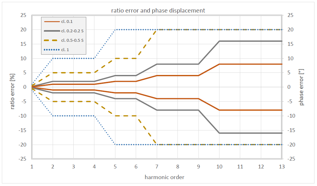
Standardization trends regarding frequency response in IEC 61869-1
Due to the increasing importance of harmonics in a wide variety of measurement applications, accuracy values for different frequency ranges are listed in the already adopted final draft (AFDIS) of IEC 61869-1. Five extension levels for the measurement of harmonics are to apply to the known accuracy classes. These are called WB0 to WB4. The extension WB0 is to be interpreted as the lowest level and is only defined up to the 13th harmonic. It is mandatory for sensors (LPITs) and SAMUs. Accordingly, the defined accuracies are not very restrictive.
Figure 7: Graphical illustration of class WB0 from nominal frequency for the known IT accuracy classes
However, the LZQJ-XC instrument transformer energy meter has a larger analog bandwidth and a sampling rate of 3.2 kHz. This means that regarding a serious active power measurement, accuracies of up to at least 5 kHz are advisable, because the high-energy pulse frequencies of wind turbines are usually between 2 and 4 kHz. In the type test of the wind turbine, the power measurement is usually carried out on the low-voltage side. The Fluxgate current transducers used for laboratory applications provide highly accurate measured values up to at least 5 kHz.10
In addition to class WB0, classes WB1 to WB4 for instrument transformers are currently defined as follows.
Figure 8: Overview of classes WB1 to WB4 according to IEC 61869-1 ED2 (AFDIS)
If the power measurement at the connection point is also to be carried out without distortion up to 5 kHz, class WB1 is not sufficient. This is only defined up to 3 kHz. Class WB2 is defined up to 20 kHz and is certainly a good choice. With regard to the bandwidth, it becomes clear that inductive or capacitive voltage transformers should no longer be used for power measurement in any case, even if only small amplitudes are to be expected at higher frequencies. Otherwise, the meter manufacturer would have to limit the analog bandwidth for active power calculation to almost nominal frequency.
In the future, the customer should be able to optionally specify the accuracy classes for harmonics according to the table shown above when ordering the instrument transformer. For example, this would result in the following specification:
Accuracy class 0.2-WB2
Technology change in voltage measurement
It can be stated that a technology change in the field of voltage measurement from 123 kV must take place if the energy meters continue to have a larger analog bandwidth than the voltage transformers. The Swiss manufacturer of high-voltage equipment CONDIS SA has responded to the need for broadband voltage transformers and offers CR dividers for the voltage range of 123 kV. The use of these sensors in billing measurement is to be evaluated as permissible in Germany and in many other countries due to the applicable regulations.
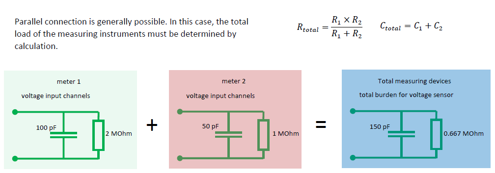
Due to the principle of operation, it is a Low Power Instrument Transformer (LPIT) in contrast to the traditionally used devices, which cannot provide the conventional power on the secondary side. However, this circumstance should not be an issue. Like the traditional devices, a signal of 100/√3 volts is also provided on the secondary side. When selecting the energy meter, it is important to ensure that the electrical supply is delivered by a separate power supply and is not provided through the voltage measurement channels. Furthermore, the meter manufacturer must specify the exact input impedance of the meter for the voltage channels. In the case of the LZQJ-XC, this results in
880.680 kOhm. In principle, it is also possible to operate meters in parallel. In this case, only the total impedance must be calculated. A value above 250 kOhm is generally considered as feasible.
Figure 9: Determination of the total impedance with two connected measuring instruments
In addition, the cable length from the sensor to the measuring devices must be specified precisely, since the impedance of the cable is also included in the calculation. In addition to energy meters, power quality analyzers can thus also be operated in parallel on one sensor.
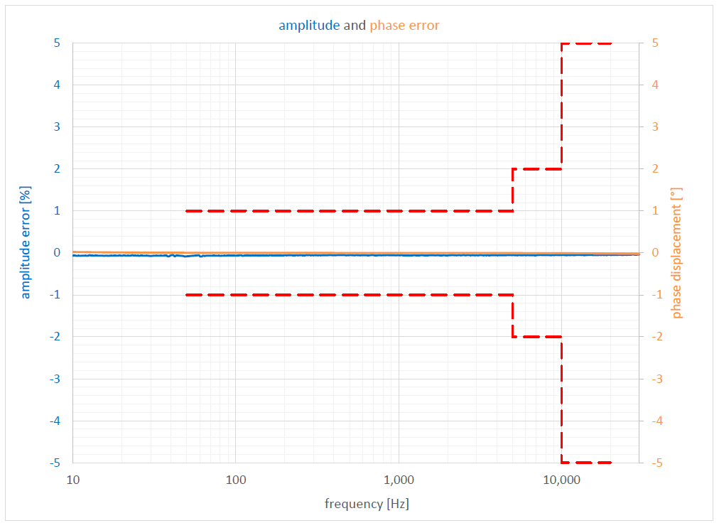
Figure 10: CR divider of CONDIS SA with frequency response up to 1 MHz. In red: allowed errors acc. cl. 0.5 – WB4
While the above CR divider is only used for power quality measurements, class 0.1 in combination with frequency class WB2 have been realized for a metering CR divider with Um=123 kV which can be used for settlement purposes.
Figure 11: Frequency response of a CR divider from the CONDIS SA up to 30 kHz. In red: allowed errors acc. cl. 0.1 – WB2
Current transformer
Like the measurement technology for voltage measurement with Um ≥ 123 kV, the technology for current measurement is also freely selectable. This also applies if a current transformer isolated to low voltage is installed at the bushings of the switchgear or power transformer. There are two reasons for this statement:
Current transformer with insulation coordination (0.72 / 3 / – kV) is only the secondary part of a instrument transformer. The complete instrument transformer is located in a system with Um ≥ 123 kV.
The primary side of the instrument transformer (here the bushing) is also specified for insulation coordination with Um ≥ 123 kV.
Here, too, the inductive current transformers described in the PTB test rules were used in the past. The secondary current ratings are specified with 1 and 5 A. Accordingly, many instrument transformer meters are equipped with 1 or 5 A current measurement inputs. If class WB2 up to 20 kHz is selected here as well, care should be taken to ensure that the manufacturer takes the connecting cable to the metering device into account when specifying class WB2 for frequency measurement. It is not uncommon for one-way lengths of 100 to 300 m to occur. At higher frequencies, the inductances and capacitances of the cable can negatively affect the accuracy at higher frequencies.
While in the literature current transformers are said to have a much better frequency response than voltage transformers, switching operations can cause the iron core to have residual magnetization. The reason for this is that the current is switched off at zero crossing. At this point, the magnetic flux density is exactly at its maximum due to the 90° shift. Particularly in the case of hard magnetic core materials without following excitation with the entire rated primary current and full burden power, the hysteresis curve does not always return to the starting point.11 The current transformer remains in a magnetic operating range which has not been specified and tested.12
Figure 12: Schematic diagram of a demagnetization process of a current transformer with hard magnetic core material
But parasitic DC currents such as GICs can also shift the magnetic operating point of current transformers. The University of Stuttgart has proven that for an investigated current transformer with the measurement class 0.2S, the accuracy class was already left at 100 mA DC.13
The company Senseleq is a joint venture of the Dutch instrument transformer manufacturer Eleq and the Danish supplier of high-precision laboratory current transducers Danisense. These current transducers are based on the fluxgate principle and are used in test laboratories of wind turbine manufacturers, among others. These precision sensors can also be supplied in traditional designs for grid applications and ensure current measurement from DC to the double-digit kHz range in the high-voltage grid. In addition to power measurement, the harmonic measurements required in many national grid standards can also be realized in this way.14
Figure 13: Fluxgate current transformers on GE’s HYpact switchgear
Among other things, the output signal of the fluxgate current transformer is 1 A at nominal current and can therefore be used with the existing instrument transformer meters on the market. Even with smaller primary currents, no major inaccuracies in amplitude or phase angle are to be expected.
Figure 14: Amplitude and phase error of a fluxgate current transducer with the ratio 2500/1 A
In addition to the high accuracy at nominal system frequency, harmonic currents up to 50 kHz can be analyzed simultaneously in the above project. A PQ analyzer from Neo Messtechnik GmbH is used for this purpose, which has a sampling rate of 1 MS/s. The loupe function in the FFT analysis can even make GICs visible in the range from 0 to 1 Hz.15
Conclusion
The latest standard proposal regarding defined bandwidths for the known accuracy classes of instrument transformers is generally welcomed. Unfortunately, regarding the defined accuracy classes for higher-frequency components, the standard proposal only refers to PQ measurements and protection applications in the area of traveling waves. Defined bandwidths should also be considered in the future for power and billing measurements. It can be assumed that in the next few years there will have to be a technology change towards broadband sensors regarding voltage measurement. Fluxgate current transducers can also meet all future measurement requirements for current measurement and guarantee significantly better accuracy than conventional current transformers, especially in billing measurement. A delay of the technology change by the responsible authorities is not to be expected for Um ≥ 123 kV. The first projects in Europe have already been realized.
Published by Michael B. Marz, American Transmission Company, Waukesha, WI Email: mmarz@atcllc.com
INTRODUCTION
The use of sophisticated power electronics and communication systems to improve power system efficiency, flexibility and reliability is increasing interharmonic distortion and adding equipment sensitive to that distortion to the system. Knowledge of interharmonics, their sources, effects, measurement, limits and mitigation, will help the industry prevent interharmonics from adversely affecting the power system.
INTERHARMONIC DEFINITIONS
The IEEE defines interharmonics as:
“A frequency component of a periodic quantity that is not an integer multiple of the frequency at which the supply system is operating (e.g., 50 Hz or 60 Hz).” 1
The IEC defines interharmonics as:
“Between the harmonics of the power frequency voltage and current, further frequencies can be observed which are not an integer of the fundamental. They can appear as discrete frequencies or as a wide-band spectrum.” 2
Simply put, interharmonics are any signal of a frequency that is not an integer multiple of the fundamental frequency. If f1 represents the fundamental frequency and n is any nonzero integer, nf1 is a harmonic of f1. For the special case when n is zero, nf1 is also zero, i.e. dc. For m, any positive non-integer number, mf1 is an interharmonic of f1. When m is greater than zero and less than one, mf1 is sometimes referred to as a subharmonic of f1. These definitions are summarized in Table 1.
Table 1 – Harmonic and Interharmonic Definitions
.
One characteristic of all periodic signals is that they can be represented by their fundamental component and a Fourier series of harmonics of various magnitudes, frequencies and angles.3 By definition interharmonics are not periodic at the fundamental frequency, so interharmonics can be thought of as a measure of the non-periodicity of a power system waveform. Similarly, any waveform that is non-periodic on the power system frequency will include interharmonic distortion.
INTERHARMONIC SOURCES
Power system interharmonics are most often created by two general phenomena. The first is rapid non-periodic changes in current and voltage caused by loads operating in a transient state (temporarily or permanently) or when voltage or current amplitude modulation is implemented for control purposes. These changes can be quite random or, depending on the process and controls utilized, quite consistent. Changes in current magnitude or phase angle can also create sidebar components of the fundamental frequency and its harmonics at interharmonic frequencies.
The second source of interharmonics is static converter switching not synchronized to the power system frequency (asynchronous switching). Thyristor switched converters are triggered into forward conducting mode and keep conducting until their current falls below its holding current. By turning off at the same voltage each cycle, thyristor devices are synchronized to the power system frequency and do not produce interharmonics. Insulated gate bipolar transistors (IGBTs), which can be turned off as well as on at any time, are replacing thyristors in converters because their greater flexibility allows for reactive as well as real power regulation and power system oscillation damping. The asynchronous switching of converters using IGBTs produces interharmonics.
Oscillations between series or parallel capacitors or when transformers or induction motors saturate can also produce interharmonics. Some specific sources of interharmonics include arcing loads, induction motors (under some conditions), electronic frequency converters, variable load drives, voltage source converters and power line communications.
Arcing Loads include arc furnaces and welding machines. For most large industrial arc furnaces, transient loading and interharmonics vary throughout the melt cycle. Load variability and the resulting interharmonics are usually greater at the beginning of the melt cycle. Welding machines produce a more continuous frequency spectrum that includes many interharmonic frequencies.
Induction Motors have slots in their stator and rotor iron that can produce interharmonics when their magnetic circuits saturate. These interharmonics can increase during startup. Motor asymmetry can also produce interharmonics. Variable torque loading can also cause motors to produce interharmonics.
Electronic Frequency Converters use a dc link to convert one frequency to another. Filtering on the dc bus is used to decouple the voltage and current on each side of the link, but this filtering is never perfect and interharmonic distortion can pass between the two ac systems.
Variable Load Dives such as traction system power supplies that use IGBTs or experience sudden load changes can produce interharmonics, usually at fixed frequencies.
Voltage Sourced Converters (VSCs) are used for a variety of applications including modern wind generator dc to ac conversion, static compensators (STATCOM) and HVDC applications. The use of IGBTs in VSCs has advantages over line commutated converters (LCC) that use thyristors. Among these advantages are the ability to independently regulate reactive power at each converter, operate under very weak system conditions and blackstart one dc terminal from the other. The ability of IGBTs to turn off at any time also allows near instantaneous control that can be used to improve system stability by damping oscillations.
One consequence of the increased control provided by VSCs is the production of interharmonics. The level of interharmonics produced by a VSC device depends on its type. Earlier types used pulse width modulation (PWM) that produced much higher interharmonics than the newer modular multilevel (MML) designs. Other types (Cascaded Two Level, etc.) also produce interharmonics. Examples of voltages produced by PWM and MML VSCs are shown in Figure 1. In addition to type, the frequency and level of interharmonics produced by a specific VSC converter depends on a number of design factors (pulse number, levels, etc.) that are chosen for reasons usually unrelated to interharmonic generation.
Figure 1 – (a) Pulse Width Modulation (PWM) and (b) Modular Multilevel MML VSC Voltage Waveforms
Power Line Communications are used by some utilities to transmit system protection information, control certain loads or reactive resources or provide two way communications to customer “smart” meters. All of these systems use non-periodic signals added to the power frequency waveform to communicate. Protection information is usually transmitted using frequencies in the 100’s of Hz range and are intended to be transmitted from one location to another and prevented from reaching the wider system by wave traps. Load or reactive resource control signals in the 100 to 3000 Hz range, sometimes called ripple control signals, reach the wider system, but are generally of low magnitude, short duration and used infrequently. Both protection and load control signals usually use a minimal number of frequencies that are meant to communicate simple instructions (trip, block, turn on or turn off). Higher frequency signals, up to the 100’s of kHz, may be used in smaller areas for commercial communication applications.
Smart meter communication over power lines have been used for a variety of purposes with varying levels of data intensity. Generally, either the current, voltage or both are briefly shorted to ground to send a step signal that is interpreted as a binary bit. Series of bits are interpreted to identify the meter and the information it is sending. Multiple meters can send signals at the same time, but with multiple communication attempts and error checking, communications can be quite reliable. These signals include a wide range of interharmonic frequencies, but their magnitude generally decreases as their frequency increases.
Interharmonics can be generated at and transferred to any voltage level. Although a relatively limited number of interharmonic measurements are available publically, low levels of interharmonics (0.01- 0.02%) have been measured at transmission level voltages with no known large interharmonic sources. Even with known interharmonic sources voltage interharmonic levels rarely exceed 0.5% of the fundamental voltage, except under resonance conditions.4 These interharmonic magnitudes are approximately an order of magnitude below applicable harmonic distortion limits.
INTERHARMONIC EFFECTS
Interharmonics, like harmonics, add additional signals to the power system. These additional signals can cause a number of effects, particularly if they are magnified by resonance. The wider the range of frequencies present, the greater the risk of resonance. Many of the effects of interharmonics are similar to those of harmonics, but some are unique to interharmonics as a result of their non-periodic nature.
Effects of interharmonics similar to those of harmonics caused by an additional signal superimposed on the fundamental can be separated into three categories: overloads, oscillations and distortion. The effects of overloads include additional energy losses that can contribute to heating, overloading filters or other system components and current transformer saturation. Depending on their frequency, these additional signals can cause oscillations in mechanical systems, acoustic disturbances, or interfere with telecommunication signals. Distortion of the fundamental frequency waveform can interfere with the operation of equipment synchronized with system zero-crossings or dependent on a consistent crest voltage, such as fluorescent lights, timing devices and some electronic equipment.
Two of the most common and impactful effects of interharmonics that are not problems with harmonic distortion are light flicker and power line communication interference, both of which require non-periodic signals to occur.
Light Flicker is caused by variations in rms voltage magnitude. The perceptibility of flicker varies with the frequency and magnitude of these voltage variations. The dependence of rms voltage variation on the frequency of a constant 0.2% amplitude interharmonic is shown in Figure 2.5 This figure shows the impact on flicker of interharmonic frequencies above the second harmonic is minimal. Virtually all types of lighting can be susceptible to flicker, but flicker intensity can vary for different types of lighting when they are exposed to voltage deviations of the same magnitude and frequency.
Figure 2: RMS Voltage Deviation with a 0.2% Distortion (50 Hz System)
Power Line Communications were discussed earlier as a source of interharmonics. Protection and ripple control signals usually consist of a single interharmonic frequency. They are usually not affected by other interharmonics that are of lower magnitude or do not match their frequency. Two way communications that rely on step changes in system voltage or current to send bits of information consist of multiple interharmonic frequencies. The interharmonic distortion created by power line communications carries information that, once the 60 Hz signal and its harmonics are removed, can be interpreted. If interharmonics from other sources are in the same frequency range as the power line communication signals, they can interfere with signal interpretation making it difficult for the power line communications to be completed.
Power line communications signals can also cause flicker. While these communication signals are designed to be too small to cause flicker, they have been known to cause very sensitive lighting (compact fluorescent with inductive ballasts) to flicker. If a power line communications system is not reliable, one fix may be to increase signal magnitude. This fix has limitations as increasing signal magnitude too much could cause flicker even in less sensitive lighting.
MEASURING INTERHARMONICS
Methods commonly used to measure the frequency components of a waveform use a phase locked loop to synchronize the measurement with the fundamental frequency. The signal is then analyzed using a Fourier Transformation (FT) of one or more cycles. This accurately represents the waveform only if it does not contain any non-periodic (interharmonic) components. The FT uses a specific measuring window (time period – T, 1/T = frequency) and a limited number of samples (M) of that window. The signal outside the window is assumed to be identical to that inside the window. For North American power system waveforms periodic at the fundamental frequency 1/T is 60 Hz and a sample of 16.67 milliseconds is sufficient to fully analyze a waveform’s harmonic frequency components. The measurement of interharmonics, which are non-integer multiples of the fundamental frequency and may vary with time is more difficult.
With interharmonic components present, the greatest common devisor of all component frequencies in a signal, the Fourier Frequency, is not the fundamental frequency and can be quite small. This can dramatically increase the minimum acceptable sampling time, required sample size and overall computational complexity. For example, a signal with a 60 Hz fundamental, a 71.2 Hz interharmonic and a 3000 Hz harmonic has a fundamental Fourier Frequency is 0.2 Hz. The corresponding period is 5 seconds and, using the Nyquist criteria, a minimum sample frequency of 12,000 Hz. This results in a sample size, frequency (12,000 Hz) times period (5 seconds), of 60,000. With no interharmonic, the minimum sample frequency would remain the same (12,000 Hz) but the minimum measurement time would be one 60 Hz cycle, 16.67 milliseconds resulting in a sample size of 200 (12,000 Hz * 0.01667 seconds). In this example, including the 71.2 Hz interharmonic increases the measurement time and sample size 300 times.
To simplify the measurement process and produce repeatable results, IEC 61000-4-76 uses a method based on the concept of grouping. For a 60 Hz system its basis is a Fourier Analysis with a 12 fundamental cycle basis that uses a phase locked loop synchronized with the fundamental frequency. This results in a spectrum with a 5 Hz resolution. Analysis details can be found in the standard.
This analysis produces harmonics at frequencies that are multiples of the fundamental and interharmonics every 5 Hz between the harmonic frequencies. These harmonic and interharmonic components can then be grouped into Harmonic Groups, Interharmonic Groups, Harmonic Subgroups and Interharmonic Subgroups (Figure 3). The magnitude of each group or subgroup is calculated by taking the square root of the sum of the squares of the components of each group or subgroup. According to IEC Standard 61000-4-7 the interharmonic group below the fundamental frequency (subharmonic) is interharmonic 0, the interharmonic group between the fundamental and second harmonic is Interharmonic 1, etc. Not all interharmonic meters follow this convention and instead label the interharmonic group below the fundamental frequency as interharmonic 1, the interharmonic group between the fundamental and second harmonic is Interharmonic 2, etc. The same calculations are used for both voltage and current.
Figure 3: Harmonic and Interharmonic Groups and Subgroups
The magnitude of any Interharmonic Group (IG) is the square root of the sum of the squares of the magnitudes of the interharmonics in that group. For example the magnitude of the second interharmonic group, or more simply the second interharmonic, shown in Figure 3 is the square root of the sum of squares of the magnitudes of the interharmonic components from 125 Hz to 175 Hz. Equation 1 is the equation used to calculate the magnitude of Interharmonic Group N, from the 11 interharmonic component magnitudes (Y) between the Nth and (N+1)th harmonics.
.
The Interharmonic Subgroup (ISG) magnitude calculation removes the interharmonic components closest to each of the harmonics from the interharmonic group calculation (Equation 2).
.
The Harmonic Group (HG) magnitude calculation includes the harmonic frequency and all of the interharmonic components closest to that harmonic frequency. Since the interharmonic components 30 Hz above and 30 Hz below each harmonic are equal distance from each harmonic, half the magnitude of both of these components are included in the calculation (Equation 3).
.
The Harmonic Subgroup (HSG) magnitude calculation includes only the harmonic frequency and the interharmonic components immediately adjacent to the harmonic frequency (Equation 4).
.
Total harmonic distortion is calculated as the square root of the sum of the squares of all individual harmonic components of significant value. Similarly, a total interharmonic distortion can be calculated by taking the square root of the sum of the squares of all interharmonic groups of significant value.
INTERHARMONIC STANDARDS, GUIDELINES AND LIMITS
The effects of interharmonics can be divided into three categories: (1) those related to flicker, (2) those similar to harmonics and (3) those affecting power line communications. Because these phenomena are different, the limits required to prevent power system issues because of each of them are also different.
IEEE Standard 519-2014 contains informative interharmonic limits designed to prevent flicker. IEC 61000-2-2: 20027 contains similar “standard compatibility levels” for “interharmonic voltages occurring at a frequency close to the fundamental (50 Hz or 60 Hz), resulting in amplitude modulation of the supply voltage.” Both standards limit the interharmonics of concern for flicker to frequencies below the second harmonic. The IEEE interharmonic voltage informative limits based on flicker are as high as 5% below 16 Hz, above 104 Hz and very close to 60 Hz. There is of course no limit at 60 Hz. The limit is as low as 0.23% at 51 Hz and 69 Hz. These informative interharmonic voltage limits are shown graphically in Figure 4. The limits in 1 Hz increments are included in tabular form in IEEE-519 (Table A-1 in Annex 1). These limits correlate to a short term flicker severity (Pst) of 1.0.
Figure 4: IEEE 519 Informative Interharmonic Voltage Limits Based on Flicker for Frequencies up to 120 Hz for 60 Hz Systems.
Beyond the interharmonic limits based on flicker, IEEE 519 provides little guidance on flicker limitations due to effects similar to those of harmonic distortion or to address power line communication issues. The standard states that “the effects of interharmonics on other equipment and systems such as generator mechanical systems, motors, transformers, signaling and communications systems, and filters” should be given “due consideration” and “appropriate interharmonic current limits should be developed on a case-by-case basis using specific knowledge of the supply system, connected user loads and provisions for future users.”
IEC 6100-2-2 states that there is not enough knowledge of interharmonics on the system for there to be agreement on compatibility limits beyond those for flicker, but provides some discussion on what those limits might look like. For issues similar to those of harmonics they suggest that the limits should be similar to harmonic limits. Specifically, they suggest each interharmonic frequency should have a reference level equal to the compatibility level for the next higher even harmonic. The IEC limits low voltage network 2nd harmonic voltages to 2%, 4th harmonic voltages to 1%, 6th and 8th harmonic voltages to 0.5% and even harmonic voltages from the 10th to 50th to (0.25*(10/h) + 0.25)%. IEEE 519 low voltage (<1 kV) harmonic voltage limits are 5% for all individual harmonics and 8% for total harmonic distortion. Even harmonic current limits for systems rated 120 V to 69 kV are more complicated; they depend on the ratio of short circuit to load current (ISC/IL) as well as frequency. These limits range from 0.075% for high frequencies (35th harmonic and above) with low short circuit ratios (<20) to 3.75% for low frequencies (below the 11th harmonic) with high short circuit ratios (>1000).
The IEC standard discusses ripple control receivers as a special case. Receivers can be expected to respond correctly to voltages as low as 0.3% of the supply voltage. Higher response levels are generally avoided, depending on frequency, because they run the risk of causing flicker. The IEC suggests limiting interharmonics near the ripple control frequency to 0.2% of the supply voltage.
An interharmonic voltage limit above 0.2% may be acceptable for wider spectrum communications systems if applied not for a single frequency, but for total interharmonic distortion. This limit would still need to be significantly below harmonic limits. Applying such limits system wide may not be practical in the presence of modern power system equipment that can produce significantly higher interharmonics. Under these circumstances, developing interharmonic limits on a case by case basis is reasonable. Unfortunately, without system wide limits, equipment and system design is difficult.
Above the 50th harmonic, whether or not a frequency is a harmonic or interharmonic has little significance. The IEC suggests limiting any frequency from the 50th harmonic to 9 kHz to 0.2% and any 200 Hz band in this range to 0.3%.
None of these suggested limits are enforceable and there is no consensus as to whether they are too conservative or too liberal. Attempts to design limits that would prevent interharmonics from damaging or causing misoperation of power system and power line communication equipment are in the early stages of development. One thing that is becoming clear is that the limits necessary to allow power line communications could be about an order of magnitude lower than those necessary to prevent flicker or harmonic related issues. The future of interharmonic limits will depend on the benefits interharmonic generating equipment provide the system verses the cost of making other equipment immune to the effects of interharmonics.
INTERHARMONIC MITIGATION
The effects of interharmonic distortion can be mitigated using three methods that are also applicable to harmonic distortion: (1) reducing emission levels, (2) reducing load sensitivity and (3) reducing the coupling between distortion generating equipment and sensitive loads. The wide band nature and variability of the interharmonic distortion emitted from certain types of loads can make all three mitigation methods more difficult for interharmonics than for harmonics.
Reducing interharmonic emission levels is difficult because reducing interharmonics could also reduce the benefits of interharmonic producing equipment such as independent var production or consumption and oscillation damping from devices with electronic controls. Interharmonics from arcing loads and welders cannot be reduced without reducing process efficiency. Similarly, reducing interharmonics from power line communications systems could reduce their effectiveness.
Reducing the sensitivity of loads to interharmonics can, in some cases, be done in ways that are similar to reducing load sensitivity to harmonics. If the additional interharmonic signal makes current overloads or voltage peaks an issue, higher rated equipment can be utilized. Timing issues created by distorted zero crossing or voltage waveforms may be able to be addressed by utilizing equipment that is not synchronized to the power system. Power line communications are more difficult to modify to make them less sensitive to interharmonic distortion. They are usually designed so that their signal strength cannot be significantly increased without risking creating flicker. While single frequency signals can be modified to avoid certain sensitive frequencies, wide spectrum signals, which carry more information, often cannot. Often the most practical solution is to remove wide spectrum communications from the power line.
Reducing the coupling of interharmonic producing devices and sensitive loads is usually done with filters. Filtering can be practical when there is a single, or a minimal number of, interharmonic frequencies of concern. When there are multiple interharmonics of varying frequencies filtering may not be practical. Passive filters use low impedances at targeted interharmonic frequencies to shunt interharmonic currents to ground. Filters, especially lower loss undamped filters, can significantly amplify non-targeted frequencies. When only a limited number of interharmonic frequencies are a concern, these amplified frequencies can be designed to avoid frequencies of concern. This may be practically impossible when a wide range of interharmonics must be filtered.
A major concern when filtering for wide spectrum power line communications is the Mvar size of the filtering necessary. Power line communications require a lower level of interharmonics to function as designed, which means larger (on an Mvar basis) filtering will be necessary. The size of the filters necessary to allow wide spectrum power communications can create unacceptable voltage regulation and cost issues.
CONCLUSIONS
The level of interharmonic distortion on the system is generally low because there are presently few large interharmonic sources on the system. This low level of interharmonics has kept interharmonic related problems relatively rare and the need to measure or mitigate interharmonics uncommon. Interharmonic measurement techniques have been standardized, but there are no mandatory standards for limiting interharmonics. If there were, these limits would likely be similar to existing harmonic and flicker limits, unless they were designed to allow power line communications, in which case they may have to be reduced by approximately an order of magnitude.
Although advances in technology that are increasing the system flexibility are increasing the level of interharmonics on the system, most power system equipment that produces interharmonics produce them at levels significantly below the limits specified for harmonics. This makes it unlikely, at the present time, that interharmonics will cause the problems associated with harmonics on most systems.
Power line communications require lower levels of interharmonics to function properly. These levels can be achieved by filtering for single frequency communications whose frequency can’t be changed, but issues with systems that produce wide band interharmonics may only be able to be resolved by eliminating the interharmonic source or removing the communications from the power lines. Wireless communications systems have been used near large interharmonic producing loads, such as industrial arc furnaces, to avoid interharmonic issues.
Today interharmonic issues are resolved on a case-by-case basis. This is reasonable considering the variety and limited number of interharmonic sources and sensitive loads. As the benefits and use of interharmonic generating equipment increases, manufacturers of interharmonic producing equipment and equipment sensitive to interharmonics will need guidelines if they are to design their equipment to be compatible with each other.
BIBLIOGRAPHY
[1] IEEE Standard 519-2014. “IEEE Recommended Practice and Requirements for Harmonic Control in Electric Power Systems,” 2014. [2] IEC 61000-2-1:1990, “Electromagnetic Compatibility (EMC) – Part 2: Environment – Section 1: Description of the Environment – Electromagnetic Environment for Low-Frequency Conducted Disturbances and Signalling in Public Power Supply Systems. First Edition May 31, 1990. [3] G. T. Heydt, Electric Power Quality, West Lafayette, IN: Stars in a Circle Publications, 1991. [4] Z. Hanzelka, A. Bien, Power Quality Application Guide 3.1.1, Harmonics Interharmonics, Copper Development Association, 2004. http://admin.copperalliance.eu/docs/librariesprovider5/power-quality-and-utilisation-guide/311-interharmonics.pdf [5] IEEE Interharmonic Task Force, CIGRE 36.05/CIGRE 2 CC02 Voltage Quality Working Group, Interharmonics in Power Systems, Task Force Working Document, December 1, 1997. http://grouper.ieee.org/groups/harmonic/iharm/ihfinal.pdf [6] IEC 61000-4-7:2002 Electromagnetic Compatibility (EMC) Part 4: Testing and Measurement Techniques Section 7: General Guide on Harmonics and Interharmonics Measurements and Instrumentation for Power Supply Systems and Equipment Connected Thereto. [7] IEC Standard 61000-2-2:2002 “Electromagnetic Compatibility (ECM) Part 2-2: Environment- Compatibility Levels for Low-frequency Conducted Disturbances and Signaling in Public Low voltage Power Supply Systems.” Second Edition 2002.
Published by Alex Roderick, EE Power – Technical Articles: Arc Flash and Overvoltage Protection, August 26, 2021.
In addition to the risk of electrical shock, other hazards are present when work is performed on or near energized electrical equipment or conductors. Two serious hazards are electrical arc flashes and electrical arc blasts.
An arc flash is a short circuit across the air. An arc blast is an explosion that happens when the surrounding air gets ionized and conductive. When insulation or isolation can no longer withstand the applied voltage, an arc flash occurs. An arc flash may occur from phase to ground or from phase to phase. The temperature of the arc flash may reach thousands of degrees and cause an arc blast. The explosion from the arc blast can spread hot gases and melting metal, damage hearing and vision, and send objects flying (see Figure 1).
Figure 1. Flash suits protect workers from the thermal energy of arc blasts. Image Courtesy of PKSAFETY
Note: According to the NFPA 70E, Standard for Electrical Safety in the Workplace, 2004 Edition, Annex K, the temperature of an arc flash can reach 35,000°F. Exposure to these very high temperatures both burns the skin and causes clothing to catch fire, aggravating the burn injury. Material and molten metal are expelled away from the arc at speeds exceeding 700 miles per hour, fast enough for shrapnel to completely penetrate the human body.
OSHA Part 1910.333 gives general requirements for safety-related work practices. OSHA inspectors also carry a copy of NFPA 70E and use it to enforce safety procedures related to arc flash. NFPA 70E gives specific guidelines on actions to be taken to comply with the general OSHA statements. The NEC® requires several types of equipment to be marked to warn qualified persons that a hazard exists (see Figure 2).
Figure 2. An arc flash warning label must be placed on any electrical equipment that may remain energized during repair or maintenance. Image Courtesy of SafetySign
The NFPA requires facility owners to perform a flash hazard analysis. A flash protection boundary must be established around electrical devices. This boundary is determined by calculations that estimate the maximum energy released and the distance that energy travels before dissipating to a safe level. Technicians working within the boundary must have appropriate personal protective equipment (PPE). The IEEE Standard 1584-2002, Guide for Performing Arc-Flash Hazard Calculations, gives procedures for determining the incident energy exposure, flash protection boundary, and level of PPE required. Incident energy is expressed in calories per centimeter squared (cal/cm2). This is a measure of the heat energy applied to a certain area of an object. The object may be a person. The flash protection boundary must be established at the point where the incident energy has fallen below 1.2 cal/cm2. It is not safe to assume that similar equipment located in different locations has the same flash protection boundary.
Overvoltage Protection
Voltage surges on a power distribution system can cause a safety hazard. A voltage surge is a higher-than-normal voltage that appears on one or more power lines for a short period of time. Voltage surges vary in voltage level and time present on power lines. One type of voltage surge is a transient voltage. A transient voltage (voltage spike) is an unwanted voltage of a very short duration in an electrical circuit. Transient voltages typically last for a very short period of time, but they are often higher in magnitude than voltage surges and are quite erratic. Transient voltages are caused by lightning strikes, unfiltered electrical components, and power being switched on and off. High transient voltages can reach thousands of volts. On a 120 V power line, a transient voltage can reach 1000 V (1 kV) or higher.
High transient voltages occur near a lightning strike or when large (very high-current) loads are shut off. For example, when a large motor (100 HP) is switched off, a transient voltage can travel down the power distribution network. An arc can be formed inside a DMM if it is connected to the system when the high transient voltage happens. Once started, the arc might induce a high-current short in the power distribution system even after the initial high transient voltage has passed. An arc blast can result from a high-current short.
The quantity of current drawn and the potential damage caused is dependent on the power distribution system’s specific location. Fuse and circuit breakers are used in all power distribution systems to set current limits. As you move farther from the main distribution panel, the current rating (size) of fuses and circuit breakers reduces. The farther away from the main distribution panel, the less probable it is that the high transient voltage will cause damage.
Overvoltage Installation Categories
The IEC 1010-1 standard defines four overvoltage installation categories in which a DMM may be used (Category I — Category IV). These categories are typically abbreviated as CAT I, CAT II, CAT III, and CAT IV (see Table 1). They determine the magnitude of transient voltage a DMM or other electrical appliance needs to withstand when used on the power distribution system. For example, a DMM or other electrical appliance used in a CAT III environment must withstand a 6000 V transient voltage without causing an arc. If the DMM or other appliance is operated on voltages above 600 V, then the DMM must withstand an 8000 V transient voltage.
Table 1. The IEC 1010 standard classifies the applications in which a DMM can be used into four overvoltage installation categories.
Category
In Brief
Examples
CAT I
Electronic
•Protected electronic equipment •Equipment connected to (source) circuits in which measures are taken to limit transient overvoltage to an appropriately low level •Any high-voltage, low-energy source derived from a high-winding-resistance transformer, such as the high-voltage section of a copier
CAT II
Single phase-connected loads
•Appliances, portable tools, and other household and similar loads •Outlets and long branch circuits •Outlets at more than 30′ (10m) from CAT III source •Outlets at more than 60′ (20m) from CAT IV source
CAT III
Three-phase distribution, including single-phase lighting
•Equipment in fixed installations, such as switchgear and polyphase motors •Bus and feeder in industrial plants •Feeders and short branch circuits and distribution panel devices •Lighting systems in larger buildings •Appliance outlets with short connections to the service entrance
CAT IV
Three-phase at utility connection, any outdoor conductors
•Refers to the origin of installation, where the low-voltage connection is made to utility power •Electric meters, primary overcurrent protection equipment •Outside and service entrance, service drop from pole to building, run between meter and panel •The overhead line to the detached building
.
If the DMM can withstand the voltage, the DMM may be damaged, but an arc does not start, and no arc blast occurs. To protect against transient voltages, protection must be built into the test equipment. For many years, the industry followed standard IEC 348. This standard has been replaced by IEC 1010. A DMM designed to the IEC 1010 standard offers a higher level of protection. A higher CAT number specifies an electrical environment with a larger short-circuit current available, higher power available, and higher voltage transients. For instance, A DMM manufactured to the CAT III standard is more resistant to higher energy transients than a DMM manufactured to the CAT II standard.
Power distribution systems are split into categories because a dangerous transient voltage, such as a lightning strike, is attenuated when it travels through the system’s impedance and system grounds. Within an IEC 1010 standard category, a higher voltage rating denotes a higher transient voltage withstanding rating. For example, a CAT III-1000 V (steady-state) rated DMM has better protection compared to a CAT III-600 V (steady-state) rated DMM. Between categories, a higher voltage rating (steady-state) might not provide higher transient voltage protection. For example, a CAT III-600 V DMM has better transient protection than a CAT II-1000 V DMM. A DMM should be chosen based on the IEC overvoltage installation category first and voltage second.
Author: Alex earned a master’s degree in electrical engineering with major emphasis in Power Systems from California State University, Sacramento, USA, with distinction. He is a seasoned Power Systems expert specializing in system protection, wide-area monitoring, and system stability. Currently, he is working as a Senior Electrical Engineer at a leading power transmission company.
Published by Lorenzo Mari, EE Power – Technical Articles: How to Improve Resistance to Ground, September 25, 2020.
Learn about the methods used to lower the resistance of a grounding electrode
When the soil resistivity is high, and the resistance to ground exceeds the required values, specific techniques are useful to decrease it. This article evaluates various methods for reducing the resistance of a grounding electrode.
There are several types of grounding electrodes, ranging from very simple to very complex, and the National Electrical Code (The NEC) requires particular methods be used.
For this exercise, we choose the most widely-used electrode type: a single ground rod. It is a long metal rod, usually copper bonded to steel, galvanized iron, or stainless steel.
Ground rods come in 240 cm (8 ft) and 300 cm (10 ft) lengths, and three diameters: 1.270 cm (1/2 in), 1.588 cm (5/8 in), and 1.905 cm (3/4 in).
The NEC requires a minimum length of 240 cm (8 ft) for rod and pipe electrodes. A measure of 240 cm is typical in residential installations and 300 cm in industrial and commercial power systems. As a rule, do not cut ground rods.
We’ll pick a length of 300 cm and the three diameters.
To calculate the theoretical resistance to ground, we’ll use the formulas developed by Herbert Bristol Dwight, an American-Canadian Electrical Engineer, and published in AIEE Transactions in December 1936.
Basic Methods to Reduce the Resistance to the Ground
If the resistance of a grounding rod is not low enough, several methods may improve it.
Increase the rod diameter, Increase the length of the rod, Use multiple rods, Treat the soil to reduce its resistivity,
To compute the resistance to ground of one rod, we use the following Dwight’s formula
.
where
R = Resistance to ground ρ = soil resistivity L = rod length a = rod radius
Note in the following paragraphs that, while standard rod thicknesses are diameters (d), Dwight’s formulas use the radius (a = d/2).
1. Increase the Rod Thickness
Let’s assume we bury a standard ground rod with L = 300 cm, and d = 1.270 cm, in soil with ρ = 10,000 Ω·cm. Using Dwight´s formula, the computed resistance is 35 Ω.
The NEC requires a supplemental electrode when the resistance to ground of a single rod exceeds 25 Ω. So, we decide to use a larger diameter rod to reduce the resistance rather than bonding supplemental electrodes. Table 1 shows the results with the three standard diameters.
Table 1 Effect of rod diameter
.
Analyzing Table 1, the minimum resistance obtained is 33 Ω, requiring a supplemental electrode.
Figure 1 shows the resistance values of the three rods in percentage of the resistance of the narrower rod.
Figure 1. Effect of rod diameter
If the soil resistivity varies, so does the ground resistance. The percentages will remain constant.
We conclude from this analysis that the rod diameter has no significant effect on the resistance to ground. The selection of a rod with a larger diameter comes only from mechanical considerations, as the rods will likely be buried using both manual and pneumatic hammers.
2. Increase the Rod’s Length
Next, let’s examine the effect of increasing the length of the grounding rod. The ground rods can be stacked and joined with a specially designed clamp to lengthen them deeper into the earth. We have chosen the larger diameter rods so that they are easier to drive into the ground.
Table 2 summarizes the effect of piling one, two, three, and four rods. As expected, driving grounding rods more deeply into the ground decreases their resistance.
Table 2 Effect of the rod’s length
.
Figure 2 shows the impact of lengthening the grounding rod, in percentage of the resistance of the shorter length. Notice the highest resistance reduction occurs when adding the first rod. Attaching more rods creates a gradually smaller percentage of reduction in resistance.
Figure 2 Effect of the rod’s length
A more in-depth analysis of Table 2 and Figure 2 allows us to establish a rule of thumb: doubling the rod’s length reduces the resistance by around 45%.
The rod driven 300 cm down has a resistance of 33 Ω, but driven 600 cm down has a resistance of 18 Ω. Applying the 45 % rule:
33 Ω ∙ 0.45 = 14.85 Ω reduction.
Then, 33 Ω – 14.85 Ω ≈ 18 Ω.
Another example show moving from from 600 cm to 1,200 cm.
From Table 2, the rod driven 600 cm down has a resistance of 18 Ω, and driven 1,200 cm down has a resistance of 10 Ω.
18 Ω ∙ 0.45 = 8.1 Ω reduction.
Then, 18 Ω – 8.1 Ω ≈ 10 Ω.
The last column of Table 2, % Reduction, should not be confused with this rule of thumb, as those percentages always refer to the shortest rod.
Dwight’s formula assumes a homogeneous soil, that is, of constant resistivity. In real life, these soils are very rare. Then, when burying the rods, we will find several layers with different resistivities. If the resistivities of the lower strata are lower than at the surface, the resistance results of the grounding electrode will be lower than those calculated in this exercise. The opposite will happen if we find higher resistivity strata.
The lower strata are usually more humid, which implies less resistivity. But this is not a fixed rule. Therefore, it is essential to make resistivity measurements and develop a soil model before designing the grounding electrode.
Furthermore, in times of low temperatures, the upper layers can freeze, taking the resistivity to infinity. The section of the ground rod in the frozen layer increases the electrode’s resistance.
3. Use of Multiple Rods
Another method to reduce the resistance to ground is to add multiple rods. In this exercise, we’ll use two rods and Dwight’s equation
.
where
s = spacing with rod dimensions: L = 300 cm, and d = 1.588 cm.
The NEC requires a minimum spacing of 180 cm (6 ft).
Table 3 summarizes the resistances of two rods for five spacing values, and Figure 3 shows the resistances in percentage of the resistance for just one rod.
Table 3 Effect of rod separation
.
Two rods driven into the ground provide parallel paths, but the rule for two resistances in parallel does not apply, i.e., the resultant resistance is not one-half of one of them.
Figure 3 Effect of rod spacing
Examining Table 3 and Figure 3, we see that the resistance decreases as the spacing increases, with a reduction from 41.61 % to 48.48 %. It is important to note that at the first spacing value, there is a large decrease in resistance, but further reductions are much smaller.
These results demonstrate that the resistance decreases as the spacing increases, hence the recommendation to space the rods further apart than the length of their immersion.
4. Treat the Soil to Decrease its Resistivity
When it is not possible to drive the grounding rods deeper, due to rocks or other causes, and adding rods does not achieve a reduction in ground resistance, chemical soil treatment is an excellent alternative.
The chemical treatment method modifies the nature of the soil around the electrodes. It takes advantage of the fact that the layers closest to the electrodes account for the highest portion of the resistance to ground. Thus, the replacement of a small volume of the original soil with one or more chemicals achieves a considerable reduction in resistance to earth.
If we use Dwight’s formula for a single grounding rod to compute the variation in resistance as a function of soil resistivity, keeping the length and radius of the rod constant, the formula reduces to
R = k∙ ρ
Thus, resistance is directly proportional to soil resistivity. This is an important result, because it demonstrates that soil resistivity strongly influences overall resistance.
Table 4 and Figure 4 show the reduction in resistance as soil resistivity decreases.
Magnesium sulfate is common because of its low cost, low resistivity, and low corrosivity. Potassium nitrate and sodium chloride are very corrosive.
This method requires maintenance by adding chemicals periodically.
The local authorities may prohibit the use of chemicals if they believe that the compounds could leach into nearby areas and cause problems.
Other useful products include:
• Charcoal • Bentonite (Natural clay)
A Review of Improving Resistance
Sometimes the resistance to the ground of an electrode turns out to be excessively high. There are several simple methods to reduce this resistance.
The most effective methods are to increase the depth of the electrode, place several electrodes, and perform a chemical treatment to the soil near the electrodes. Increasing the diameter of the ground rod does not result in a significant reduction in resistance to ground.
The best solution depends on the particular case. The chemical treatment method should be used with caution due to the potential problems of corrosion and environmental contamination.
This exercise involves a very simple grounding electrode. The conclusions, however, also apply to more complex electrodes.
Author: Lorenzo Mari holds a Master of Science degree in Electric Power Engineering from Rensselaer Polytechnic Institute (RPI). He has been a university professor since 1982, teaching topics as electric circuit analysis, electric machinery, power system analysis, and power system grounding. As such, he has written many articles to be used by students as learning tools. He also created five courses to be taught to electrical engineers in career development programs, i.e., Electrical Installations in Hazardous Locations, National Electrical Code, Electric Machinery, Power and Electronic Grounding Systems and Electric Power Substations Design. As a professional engineer, Mari has written dozens of technical specifications and other documents regarding electrical equipment and installations for major oil, gas and petrochemical capital projects. He has been EPCC Project Manager for some large oil, gas & petrochemical capital projects where he wrote many managerial documents commonly used in this kind of works.
Published by Electrical Installation Wiki, Chapter M. Power harmonics management – Essential indicators of harmonic distortion and measurement principles
A number of indicators are used to quantify and evaluate the harmonic distortion in current and voltage waveforms, namely:
• Power factor • Crest factor • Harmonic spectrum • R.m.s. value
These indicators are indispensable in determining any necessary corrective action.
Harmonic distortion indicators – Power factor
The power factor λ is the ratio of the active power P (kW) to the apparent power S (kVA).
The Power Factor must not be mixed-up with the Displacement Power Factor (cos φ), relative to fundamental signals only.
As the apparent power is calculated from the r.m.s. values, the Power Factor integrates voltage and current distortion.
When the voltage is sinusoidal or virtually sinusoidal (THDu ~ 0), it may be said that the active power is only a function of the fundamental current. Then:
Figure M6 shows a graph of λ/cosφ as a function of THDi, for THDu ~ 0.
Fig. M6 – Variation of λ/cosφ as a function of THDi, for THDu ~ 0
Harmonic distortion indicators – Crest factor
The crest factor is the ratio between the value of the peak current or voltage(IM or UM) and its r.m.s. value.
• For a sinusoidal signal, the crest factor is therefore equal to √2. • For a non-sinusoidal signal, the crest factor can be either greater than or less than √2.
The crest factor for the current drawn by non-linear loads is commonly much higher than √2. It is generally between 1.5 and 2 and can even reach 5 in critical cases.
A high crest factor signals high current peaks which, when detected by protection devices, can cause nuisance tripping
Examples:
Figure M7 represents the current absorbed by a compact fluorescent lamp.
Fig. M8 – Typical voltage waveform in case of high impedance line supplying non-linear loads
Harmonic spectrum
The harmonic spectrum is the representation of the amplitude of each harmonic order with respect to its frequency.
Figure M9 shows an example of harmonic spectrum for a rectangular signal.
Each type of device causing harmonics draws a particular form of current, with a particular harmonic content. This characteristic can be displayed by using the harmonic spectrum.
Fig. M9 – Harmonic spectrum for a rectangular signal U(t)
R.m.s. values
The r.m.s. value of voltage and current can be calculated as a function of the r.m.s. value of the various harmonic components:
.
Usefulness of the various indicators of Harmonic distortion
THDu is an indicator of the distortion of the voltage wave.
Below are given indicative values of THDu and the corresponding consequences in an installation:
• ≤ 5%: normal situation, no risk of malfunctions, • 5 to 8%: significant harmonic distortion, some malfunctions are possible, • ≥ 8%: major harmonic distortion, malfunctions are probable. In-depth analysis and the installation of mitigation devices are required.
THDi is an indicator of the distortion of the current wave.
The current distortion can be different in the different parts of an installation. The origin of possible disturbances can be detected by measuring the THDi of different circuits.
Below are given indicative values of THDi and the corresponding phenomena for a whole installation:
• ≤ 10%: normal situation, no risk of malfunctions, • 10 to 50%: significant harmonic distortion with a risk of temperature rise and the resulting need to oversize cables and sources, • ≥ 50%: major harmonic distortion, malfunctions are probable. In-depth analysis and the installation of mitigation devices are required.
Power factor λ is used to determine the rating for the different devices of the installation.
Crest factor is used to characterise the aptitude of a generator (or UPS) to supply high instantaneous currents. For example, computer equipment draws highly distorted current for which the crest factor can reach 3 to 5.
Harmonic spectrum provides a different representation of electrical signals and can be used to evaluate their distortion.
Author: This Electrical Installation Wiki is a collaborative platform, brought to you by Schneider Electric: our experts are continuously improving its content, collaboration is also open to all.
The Electrical Installation Guide (wiki) has been written for electrical professionals who must design safe and energy efficient electrical installation, in compliance with international standards such as the IEC 60364.
Published by Arif Nur AFANDI1,2,3, Irham FADLIKA1, Langlang GUMILAR1, Takeshi HIYAMA4
1Electrical Engineering, Universitas Negeri Malang, Malang, Indonesia 2Center for Advanced Materials for Renewable Energy, Universitas Negeri Malang, Malang, Indonesia 3Smart Power and Advanced Energy Systems Research Center, Batu, Jawa Timur, Indonesia 4The IROAST, Kumamoto University, Kumamoto, Japan
Abstract. Based on current developments related to the application of technology and the growth of load demand, power system structure (PSS) has grown into a large, intelligent network by integrating many new systems. At present, many classical systems are being modernized and developed towards smart systems to various technical performances while providing continuously energy from the generating sites to serve load centres as end energy users. On the other hand, protection and attention to the environment and renewable energy sources also affect the power system operation which is intended to reduce emissions and include green energy sources. Furthermore, these works explore an assessment of operations on local interconnection system topologies which are installed captive power plants. These studies are used to develop and evaluate the performance, where solar power plants are also installed as sources of energy suppliers. In this study, operating assessments are approached using a power flow study (PFS) to define structural performance expanded through several scenarios. In addition, the procedure for obtaining optimal conditions is also facilitated by using the Takagi Method (TM) and Thunderstorm Algorithm (TA) for PFS hybrid structures considered an integrated renewable energy source (IRES). Based on the technical scenario set, the results show that the applied scenarios have different performances. In addition, this study also provides various implications. IRES has affected system performance. PSS contributes to the part that is committed to covering the burden. TM and TA can be applied to the hybrid PFS structure.
Streszczenie. W artykule przedstawiono metodę PFS (power flow study) do optymalizacji struktury lokalnej sieci zasilającej z zainstalowanymi źródłami fotowoltaicznymi. Zastosowano też metodę Takagi i algorytm burzowy do optymalizacji sieci z różnymi scenariuszami. . Analiza pracy lokalnej sieci z uwzględnieniem własnych źródeł energii i możliwości rozbudowy
Keywords: operation, performance, power flow, structure. Słowa kluczowe: lokalna sieć zasilająca, własne (captive) źródła energii
Introduction
In principle, the power system (PS) is related to the process of converting primary energy sources and consumers as users of converted energy. So far, the energy conversion process has been carried out with applied technology which is now able to convert natural resources into a type of energy that can be used through a series of certain processes in the generating unit. On the other hand, power systems are prepared with various levels of electricity network services to form interconnection networks that connect generating units and load centers. In general, an integrated network power system (INPS) is widely used to integrate all sections [1], [2]. At present, INPS is a large network and consists of complex integrated companies and operators to control operations [3]–[6]. In general, this system is used to maintain the availability and adequacy of sustainable energy as long as customers use utilities [7]–[11]. In addition, this network is also used to combine all generating units located close to various primary energy sources. In addition, this network is also connected to the load center at different distances for power delivery.
Nowadays, the INPS is displayed by integrating a local power grid (LPG) to increase the guarantee of performances [12]–[15]. On the other hand, LPG continues to look for applied technologies as well as acceptable for the operation. Technically, LPG is operated in the classification structure which is used to supply power demands in accordance with the connections at backbone systems [2]. In particular, customers are growing faster with increasing power demand, thus, it is requiring a different generation system area with the addition of a power plant. To cover this condition, the power balance must be acceptable for energy producers and users with a reasonable low cost [16]–[19]. Increased PS operation that is guaranteed based on LPG performance is an important aspect of the level of system deviation, so as not to experience blackouts. One of the most sensitive problems of this condition is identified using shift factors and uninterrupted conditions. The most critical aspect of this other situation is related to the severity of the PS presented in generator outages, loading of transmission lines, and the magnitude of bus voltage drop.
Moreover, the operation is carried out sustainably and continuously to maintain quality and performance under the technical constraints and environmental conditions by maintaining the quality of daily operations. In addition, operations need to give double attention to dealing with complex operational problems and to include high requirements [20], [21]. INPS is also monitored and controlled in steady and transient conditions, as well as to define the power system performance (PSP) [11], [22], [23]. In addition, the contingency problem is also recognized by the power flow study (PFS) to immediately overcome the impact of faulted lines, including connected or disconnected connections, integrated and host load generators, and load changes. In detail, the system should be identified in technical indicators and it needs to maintain regularly on normal and fault conditions.
Presently, many approaches have been proposed and have been implemented to measure technical performances, including INPS and LPG. In line with the development of infrastructure and services, demand for expenses is growing in line with the availability of the produced power and the capacity of the INPS network, although load growth is faster than the provision of power plants. Therefore, the provision of power will face the possibility of exploring primary energy sources as an alternative energy source. Regarding the protection of the environment and non-fossil energy sources, renewable energy is an energy source that is an opportunity to be developed and this implementation depends on the technological readiness currently applied [19], [21], [24]– [27]. In this case, an integrated renewable energy source (IRES) is involved in the power system which is performed in an assessment of the operation of INPS, as part of the system development.
Operating
Performances In general, the assessment is used to identify system conditions throughout technical performances evaluation using operational indicator for determining the operating status under all requirements, as in previous research studies [28], [29]. Many PFS techniques have been proposed and applied to evaluate INPS and LPG. The most popular approach which widely applied is a Newton Raphson Method (NRM) and it has applied to various technical problems for power system calculations [30], [31]. Recently, PFS become an important review for presenting the performance of the electricity network. The basic equation for PFS is built in its entirety and comes from the nodal analysis equation for PSP. In detail, each bus in PS is classified into three types of load buses, bus generators, and swing buses [26], [30], [32].
In detail, the load bus referred to in the P-Q bus is defined as a bus where real and reactive power is determined and determined, while the bus voltage will be calculated and is the result of system conditions. In addition, many methods have been proposed and applied to find the optimal PFS solution as a description of the system performance is evaluated. In this study, PFS will be combined with the Thunderstorm Algorithm (TA) and the Takagi Method (TM). The structure and intelligent TA agents are discussed fully in previous works while TM effectiveness for PFS is also reported clearly in [25], [33], [34].
Fig.1. The SUMPG backbone connection
Recently, the use of fossil fuels is faced with environmental requirements and also meets the requirements of safety, reliability, and quality. In addition, commercially available energy storage systems are currently not technically or economically feasible for mass energy storage that includes the IRES [24], [26], [32], [35]. From this economic perspective, renewable energy sources become competitive icons in terms of costs compared to fossil-based energy sources [18], [25], [32], [34], [36]. This inclusion is an opportunity for PSP as part of a combination of energy supply. Based on the IRES, PFS is approached by using power injection into the system where the captive power plant (CPP) is also injected into the system.
Moreover, this PFS is used to determine steady-state performance in certain power plants from CPP-based on developed solar power plants. Therefore, PFS is designed to determine technical performance, for example, voltage, current, power loss, real power, and reactive power included in the system under the limits and requirements for the given load conditions [11], [26], [31], [37]. This assessment is very important in LPG role plays [31], [38]. Many PFS techniques are introduced to implement and assess power system performances.
In these studies, NRM is facilitated by using TM and TA to complete LPG assessments. To cover LPG interactions, the power system infrastructure development (PSID) is a very important part of exploring [1], [39]. In fact, the power system performance has presented the system in many voltage levels which are gained in indicators as well as parameters for operating status. PSID is imposed to expand the classical system from the State University of Malang Power Grid (SUMPG). In detail, SUMPG is illustrated in Figure 1. Operationally, this system is connected to the main Java Bali Power Grid (JBPG) network connected in the Malang Raya City Power Grid (MRCPG) which is established using 150 kV. In this electricity network, MRCPG supplies to Malang Regency, Malang City, and Batu City for the main areas. All cities are linked in a 150 kV system as interconnecting backbones through several other network systems of 70 kV, 20 kV and 220 V. Regarding JBPG, MRCPG is operated in two ways namely to export and import energy which is the main source of point connections. Refer to the interconnection of JBPG and MRCPG, SUMPG is supplied using 20 kV for existing local networks distributed to several main load centers. Now, SUMPG is growing and is facing increasing loads as end-energy users and is indicating that it needs infrastructure improvements and new opportunities in the main power supply system. This system also requires a backbone level of improvement to maintain performances. In these works, SUMPG is designed for the 70 kV expansion system.
Power Grid Development
As mentioned before that the PS is constructed simply in a line networking for energy productions and energy users, which is now becomes a large network and it is presented in INPS to cover the LPG area. Recently, The PSID meets a demand growth during the operating time. Moreover, an additional generating capacity, power line strengthening, and system expansion are major issues which are should be covered for the existing condition in high reliabilities. In this study, SUMPG is expanded in several additional load blocks as given in Figure 3 and designed in Figure 2.
Fig.2. Local power grid development concept of the SUMPG
According to Figure 2 and Figure 3, the SUMPG topology is developed based on two sub-systems which were approached using a 16 bus system, where three energy suppliers are applied as available resources. In detail, this system is also arranged using 17 lines; 9 load buses, and 2 solar energy centers. This topology is modified from an old structure designed based on an existing system, which is presented as a square type on the bottom side of Figure 3. Specifically, SUMPG is LPG from MRCPG which is connected to JBPG at 150 kV. In detail, the load block is concentrated on the selected 20 kV bus to integrate local load connections. This load is given in Table 1 for Ring 1 and Ring 2. In total, LPG has 15.55 MVA which is covered in 14,949 kW and 7,100 kVar.
Fig.3. Ring connecting development of the SUMPG
Table 1. Partial loads of the sub-systems
.
In particular, LPG is rearranged using a double area for Ring 1 and Ring 2, while CPP is installed in certain buses which have been determined based on the ratio of reality. Refer to the 20 kV backbone system, Ring 1 is developed to modify the radial system into a mesh form of the system. This type is redesigned from the original topology which includes all incoming electricity networks. Ring 1 integrates all load buses in partial locations. Future developments and potential sources are required to be plotted in Ring 2. Ring 2 is developed from Ring 1 by completing the IRES at the specified location for the CPP. In these locations, the CPP is presented as a solar power plant (SPP) installed on Bus 6 and Bus 9.In general, PSID is built using several electrical connection lines which are used to place two buses. This connection is also used to search for distributed power plants that are installed tightly in the load center [19], [40], [41]. In addition, the inclusion of CPP presented in SPP ensures a decrease in dependence on fossil fuels. SPP integration should contribute to the commitment of the electricity production unit. This SPP contribution also increases energy reserves and system capabilities [42], [43].
Assessing Procedures
As illustrated in Figure 2 and Figure 3, the LPG structure is divided into two areas, namely Ring 1 and Ring 2. SPP is installed in selected potential buses, where it is related to the IRES area which is designed based on the potential primary energy. In this work, the system is assessed in several case studies related to technical requirements and environmental constraints. In detail, this assessment is included in several operating scenarios, namely normal operation (NO), Ring 1 operation (R1O), Ring 2 operation (R2O). In normal operation, the system presents both rings without IRES. Ring 1 operations are focused on the circle shape of the topology structure with an open loop for Ring 2. Ring 2 operations are carried out by releasing Ring 1 so that it forms a radial type with an open circle shape as being the topology structure. By considering the disruption to the electricity network, the assessment is designed to state certain disturbances that have an impact on the breakdown of the electricity grid line. Furthermore, the termination of power production is displayed by means of operation off as it is now, that is the power grid 1 off (G1off), the power grid 2 off (G2off), and the power grid 3 off (G3off).
Fig. 4. Procedures of the power grid evaluation
In particular, the assessment procedure for evaluating the system is shown in Figure 4. This figure illustrates all the steps to find out the optimal performance based on NO, R1O, R2O, G1off, G2off, and G3off. In addition, TM is applied to the PSP by applying PFS, as detailed in [33], [44]. In this study, the implementation of TM is referred to the previous work [45], [46]. Technically, PFS is limited by several requirements. Power delivery is also constrained using technical limits for the export-import (Exim) system. In these works, TA refers to procedures and hierarchies as detailed in [25], [32]. In addition, the performance of TA and TM is not explored in these works but it is concerned in the PSP through LPG link to SUMPGS for these studies. Computationally, TA and TM performance is only used in the entire process.
Results and Discussions
In this section, this work is intended to assess PSP based on the development of topological structures and to advance the electricity system in the development of SUMPG. This system is developed in a 20 kV system as well as the operating system of its formation. This evaluation is inline with previous works [31], [38], [47], [48]. In this work, LPG is expanded in the 16 bus system model, which includes local buses designed for load blocks in Ring 1 and Ring 2. Regarding the operational scheme, PFS is analyzed using NRM, where NRM is prepared using TM and TA. From the process, the optimal results of the process are presented in normal operation, Conditions of G1off, G2off, and G3off.
In addition, Table 2, Table 3, Table 4, and Table 5 show results of the evaluation subjected the LPG. These results are given for measuring performances in several parameters that corresponded to the power grid expansion. Another results are illustrated in Figure 5 related to demands which are presented based on the scenario.
Table 2. System performances of the ring assessment scenario
.
Table 3. Power flow performances of the ring assessment scenario
.
Fig.5. Total power load under partial scenarios
Fig.6. Total generated power under partial scenarios
Fig.7. Total power loss under partial scenarios
Fig.8. Power delivery on the lines
Fig.9. Voltage drops of interconnected lines
Fig.10. The active power loss of the interconnected lines
Focused on the power production, Figure 6 gives information for partial contributions in the operation while the power loss is depicted in Figure 7. In addition, the system also has different performance, as well as every assessment applied to the system model reflecting to normal R1O, R2O, and other schemes. In general, the Exim is presented in Table 3 and Table 6 for the power delivery between each pair of buses. This table also shows a charging map for each load block. Furthermore, power delivery, voltage drop, loss are given in Figure 8, Figure 9, and Figure 10.
Table 4. System performances of the grid assessment scenario
.
Table 5. Power flow performances of the grid assessment scenario
.
Refer to Figure 8, Figure 9, and Figure 10, it can be seen that each power delivery has different characteristics and profiles. According to Exim tracking, the highest power transaction is partially generated by the G3off operation, as illustrated in Figure 8. This characteristic is also supported by Table 5 where power delivery includes 27.48 MW and 15.68 Mvar for tracking Exim 14 or the line B8 to B11. Typically, LPG provides the power around 38.48 MW and 22.05 Mvar to meet load demand at 38.32 MW and 21.84 Mvar. Other contributions are given in Table 2, Table 3, and Table 4 for all scenarios, respectively. Regarding the system performance, the voltage drop is explained in Figure 2 and Table 4. In particular, the highest decrease occurred the line B2 to B8 for all types of valuations. This condition is in line with power loss as illustrated in Figure 10, which occurs in Exim 2 which is the highest power loss.
Conclusions
This paper presents the development of a local electricity network based on operational assessment of system performances, where the local system is expanded using the 16 bus model approach and integrating potential energy resources. On the other hand, the study also refers to loading systems designed through load center blocks. Furthermore, these works show that solar power plants affect to the power production and have an effect on system performances. Each scheme has different implications on results. TM and TA have the opportunity to be applied to the evaluation of power flow. For future work, uncovering the computational structure and power transactions is recommended
Acknowledgment
The authors gratefully acknowledge the support of Universitas Negeri Malang, Malang, Indonesia, for the PNBP Research Gran
REFERENCES
[1] Z. Q. Bo, X. N. Lin, Q. P. Wang, Y. H. Yi, and F. Q. Zhou, “Developments of power system protection and control,” Prot Control Mod Power Syst, vol. 1, no. 1, p. 7, Dec. 2016. [2] P. Cuffe and A. Keane, “Visualizing the Electrical Structure of Power Systems,” IEEE Systems Journal, vol. 11, no. 3, pp. 1810–1821, Sep. 2017. [3] A. N. Afandi, “Solving Combined Economic and Emission Dispatch Using Harvest Season Artificial Bee Colony Algorithm Considering Food Source Placements and Modified Rates,” International journal on electrical engineering and informatics, vol. Vol. 6, p. 267, Jul. 2014. [4] N. S. da Silva, A. Simões Costa, K. A. Clements, and E. Andreoli, “Simultaneous estimation of state variables and network topology for power system real-time modeling,” Electric Power Systems Research, vol. 133, pp. 338–346, Apr. 2016. [5] M. Aien, A. Hajebrahimi, and M. Fotuhi-Firuzabad, “A comprehensive review on uncertainty modeling techniques in power system studies,” Renewable and Sustainable Energy Reviews, vol. 57, pp. 1077–1089, May 2016. [6] A. N. Afandi and H. Miyauchi, “Improved artificial bee colony algorithm considering harvest season for computing economic dispatch on power system,” IEEJ Trans Elec Electron Eng, vol. 9, no. 3, pp. 251–257, May 2014. [7] S. Hr. A. Kaboli, J. Selvaraj, and N. A. Rahim, “Long-term electric energy consumption forecasting via artificial cooperative search algorithm,” Energy, vol. 115, pp. 857–871, Nov. 2016. [8] B. Zakeri and S. Syri, “Electrical energy storage systems: A comparative life cycle cost analysis,” Renewable and Sustainable Energy Reviews, vol. 42, pp. 569–596, Feb. 2015. [9] A. N. Afandi, “Weighting Factor Scenarios for Assessing the Financial Balance of Pollutant Productions and Fuel Consumptions on the Power System Operation,” Wseas Transactions On Business And Economics, vol. 14, 2017. [10] A. N. Afandi, I. Fadlika, and Y. Sulistyorini, “Solution of dynamic economic dispatch considered dynamic penalty factor,” in 2016 3rd Conference on Power Engineering and Renewable Energy (ICPERE), 2016, pp. 241–246. [11] A. N. Afandi et al., “Designed Operating Approach of Economic Dispatch for Java Bali Power Grid Areas Considered Wind Energy and Pollutant Emission Optimized Using Thunderstorm Algorithm Based on Forward Cloud Charge Mechanism,” International Review of Electrical Engineering (IREE), vol. 13, p. 59, Feb. 2018. [12] J. Geeganage, U. D. Annakkage, T. Weekes, and B. A. Archer, “Application of Energy-Based Power System Features for Dynamic Security Assessment,” IEEE Transactions on Power Systems, vol. 30, no. 4, pp. 1957– 1965, Jul. 2015. [13] A. N. Afandi, “Optimal scheduling power generations using HSABC algorithm considered a new penalty factor approach,” in The 2nd IEEE Conference on Power Engineering and Renewable Energy (ICPERE) 2014, 2014, pp. 13–18. [14] F. Luo et al., “Advanced Pattern Discovery-based Fuzzy Classification Method for Power System Dynamic Security Assessment,” IEEE Transactions on Industrial Informatics, vol. 11, no. 2, pp. 416–426, Apr. 2015. [15] H. Gharavi, M. M. Ardehali, and S. Ghanbari-Tichi, “Imperial competitive algorithm optimization of fuzzy multi-objective design of a hybrid green power system with considerations for economics, reliability, and environmental emissions,” Renewable Energy, vol. 78, pp. 427–437, Jun. 2015. [16] A. N. Afandi and Y. Sulistyorini, “Thunderstorm Algorithm for Determining Unit Commitment in Power System Operation,” Journal of Engineering and Technological Sciences, vol. 48,no. 6, pp. 743–752, Dec. 2016. [17] M. Pandit, L. Srivastava, and M. Sharma, “Environmental economic dispatch in multi-area power system employing improved differential evolution with fuzzy selection,” Applied Soft Computing, vol. 28, pp. 498–510, Mar. 2015. [18] A. N. Afandi, Optimal Solution of the EPED Problem Considering Space Areas of HSABC on the Power System Operation, vol. 7. 2015. [19] N. Tutkun, O. Can, and A. N. Afandi, “Low cost operation of an off-grid wind-PV system electrifying residential homes through combinatorial optimization by the RCGA,” in 2017 5th International Conference on Electrical, Electronics and Information Engineering (ICEEIE), 2017, pp. 38–42. [20] V. M. More and V. K. Chandrakar, “Power system performances improvement by using static synchronous series compensator,” in 2016 2nd International Conference on Advances in Electrical, Electronics, Information, Communication and Bio-Informatics (AEEICB), 2016, pp. 198–201. [21] A. N. Afandi, Y. Sulistyorini, H. Miyauchi, G. Fujita, X. Z. Gao, and M. El-Shimy, “The Penetration of Pollutant Productions on Dynamic Generated Power Operations Optimized Using a Novel Evolutionary Algorithm,” International Journal on Advanced Science, Engineering and Information Technology, vol. 7, no. 5, pp. 1825–1831, Oct. 2017. [22] G. Lammert et al., “Impact of fault ride-through and dynamic reactive power support of photovoltaic systems on short-term voltage stability,” in 2017 IEEE Manchester PowerTech, 2017, pp. 1–6. [23] Z. Liu and Z. Zhang, “Quantifying transient stability of generators by basin stability and Kuramoto-like models,” in 2017 North American Power Symposium (NAPS), 2017, pp. 1–6. [24] A. Ganapathy, G. Soman, G. M. VM, and R. Lekshamana, “Online Energy Audit and Renewable Energy Management System,” in 2016 International Conference on Computing Communication Control and automation (ICCUBEA), 2016, pp. 1–6. [25] A. N. Afandi, “Thunderstorm Algorithm for Assessing Thermal Power Plants of the Integrated Power System Operation with an Environmental Requirement,” International Journal of Engineering and Technology, vol. 8, pp. 1102–1111, Apr. 2016. [26] M. EL-Shimy, N. Mostafa, A. N. Afandi, A. M. Sharaf, and M. A. Attia, “Impact of load models on the static and dynamic performances of grid-connected wind power plants: A comparative analysis,” Mathematics and Computers in Simulation, Feb. 2018. [27] D. Arengga, W. Agustin, Y. Rahmawati, S. Sendari, and A. N. Afandi, “SPEKTRA fast and smart software for renewable energy management,” IOP Conf. Ser.: Earth Environ. Sci., vol. 105, no. 1, p. 012077, Jan. 2018. [28] W. Liu, R. Cheng, Y. Xu, and Z. Liu, “Fast reliability evaluation method for composite power system based on the improved EDA and double cross linked list,” Transmission Distribution IET Generation, vol. 11, no. 15, pp. 3835–3842, 2017. [29] S. Zhao and C. Singh, “A reliability evaluation method for line switching operations in power systems,” in 2016 Power Systems Computation Conference (PSCC), 2016, pp. 1–7. [30] S. Chatterjee and S. Mandal, “A novel comparison of gaussseidel and newton- raphson methods for load flow analysis,” in 2017 International Conference on Power and Embedded Drive Control (ICPEDC), 2017, pp. 1–7. [31] J.-J. Deng and H.-D. Chiang, “Convergence Region of Newton Iterative Power Flow Method: Numerical Studies,” Journal of Applied Mathematics, 2013. [Online]. Available: https://www.hindawi.com/journals/jam/2013/509496/.%5BAccessed: 18-Mar-2018]. [32] A. N. Afandi, Y. Sulistyorini, G. Fujita, N. P. Khai, and N. Tutkun, “Renewable energy inclusion on economic power optimization using thunderstorm algorithm,” in 2017 4th International Conference on Electrical Engineering, Computer Science and Informatics (EECSI), 2017, pp. 1–6. [33] H. M. Hasanien and S. M. Muyeen, “A Taguchi Approach for Optimum Design of Proportional-Integral Controllers in Cascaded Control Scheme,” IEEE Transactions on Power Systems, vol. 28, pp. 1636–1644, May 2013. [34] A. N. Afandi and Y. Sulistyorini, “Thunderstorm Algorithm for Determining Unit Commitment in Power System Operation,” Journal of Engineering and Technological Sciences, vol. 48, no. 6, pp. 743–752, Dec. 2016. [35] M. El-Shimy, M. A. Attia, N. Mostafa, and A. N. Afandi, “Performance of grid-connected wind power plants as affected by load models: A comparative study,” in 2017 5th International Conference on Electrical, Electronics and Information Engineering (ICEEIE), 2017, pp. 1–8. [36] A. N. Afandi, I. Fadlika, and A. Andoko, “Comparing Performances of Evolutionary Algorithms on the Emission Dispatch and Economic Dispatch Problem,” TELKOMNIKA (Telecommunication Computing Electronics and Control), vol. 13, no. 4, pp. 1187–1193, Dec. 2015. [37] M. A. Elizondo, F. K. Tuffner, and K. P. Schneider, “Three-Phase Unbalanced Transient Dynamics and Powerflow for Modeling Distribution Systems With Synchronous Machines,” IEEE Transactions on Power Systems, vol. 31, no. 1, pp. 105–115, Jan. 2016. [38] Z. Ren, K. Wang, W. Li, L. Jin, and Y. Dai, “Probabilistic Power Flow Analysis of Power Systems Incorporating Tidal Current Generation,” IEEE Transactions on Sustainable Energy, vol. 8, no. 3, pp. 1195–1203, Jul. 2017. [39] X. Luo, J. Wang, M. Dooner, and J. Clarke, “Overview of current development in electrical energy storage technologies and the application potential in power system operation,” Applied Energy, vol. 137, pp. 511–536, Jan. 2015. [40] Y. Menchafou, H. E. Markhi, M. Zahri, and M. Habibi, “Impact of distributed generation integration in electric power distribution systems on fault location methods,” in 2015 3rd International Renewable and Sustainable Energy Conference (IRSEC), 2015, pp. 1–5. [41] F. S. Abu-Mouti and M. E. El-Hawary, “Optimal Distributed Generation Allocation and Sizing in Distribution Systems via Artificial Bee Colony Algorithm,” IEEE Transactions on Power Delivery, vol. 26, no. 4, pp. 2090–2101, Oct. 2011. [42] N. Gupta, A. Swarnkar, and K. R. Niazi, “Distribution network reconfiguration for power quality and reliability improvement using Genetic Algorithms,” International Journal of Electrical Power & Energy Systems, vol. 54, pp. 664–671, Jan. 2014. [43] A. Mohamed Imran and M. Kowsalya, “A new power system reconfiguration scheme for power loss minimization and voltage profile enhancement using Fireworks Algorithm,” International Journal of Electrical Power & Energy Systems, vol. 62, pp. 312–322, Nov. 2014. [44] S. R. Karnik, A. B. Raju, and M. S. Raviprakasha, “Genetic Algorithm Based Robust Power System Stabilizer Design Using Taguchi Principle,” in 2008 First International Conference on Emerging Trends in Engineering and Technology, 2008, pp. 887–892. [45] “Taguchi’s method for probabilistic three-phase power flow of unbalanced distribution systems with correlated Wind and Photovoltaic Generation Systems – ScienceDirect.” [Online]. Available: https://www.sciencedirect.com/science/article/pii/S096014811731011X. [Accessed: 11-Apr-2018]. [46] “Improving the quality of an optimal power flow solution by Taguchi method – ScienceDirect.” [Online].Available:https://www.sciencedirect.com/science/article/pii/014206159591406A. [Accessed: 11-Apr-2018]. [47] T. Kulworawanichpong, “Simplified Newton–Raphson power flow solution method,” International Journal of Electrical Power & Energy Systems, vol. 32, no. 6, pp. 551–558, Jul. 2010. [48] R. Muzzammel, M. Ahsan, and W. Ahmad, “Non-linear analytic approaches of power flow analysis and voltage profile improvement,” in 2015 Power Generation System and Renewable Energy Technologies (PGSRET), 2015, pp. 1–7.