Power Quality Blog

Harmonics Generation, Propagation and Purging Techniques in Non-Linear Loads

Published by Hadeed Ahmed Sher, Khaled E. Addoweesh and Yasin Khan

1. Introduction

Industrial revolution has transformed the whole life with advanced technological improvements. The major contribution in the industrial revolution is due to the availability of electrical power that is distributed through electrical utilities around the world. The concept of power quality in this context is emerging as a “Basic Right” of user for safety as well as for uninterrupted working of their equipment. The electricity users whether domestic or industrial, need power, free from glitches, distortions, flicker, noise and outages. The utility desires that the users use good quality equipment so that they do not produce power quality threats for the system. The use of power electronic based devices in this industrial world has saved bounties in term of fuel and power savings, but on the other hand has created problems due to the generation of harmonics. Both commercial and domestic users use the devices with power electronics based switching that draw harmonic current. This current is a dominant factor in producing the harmonically polluted voltages. The “Basic Right” of the user is to have a clean power supply, whereas the demand of utility is to have good quality instrument/equipment. This makes power quality a point of common interest for both the users as well as the utility. Harmonics being a hot topic within power quality domain has been an area of discussion since decades and several design standards have been devised and published by various international organizations and institutions for maintaining a harmonically free power supply. In a wider scenario, the harmonically free environment means that the harmonics generated by the devices and its presence in the system is confined in the allowable limits so that they do not cause any damage to the power system components including the transformers, insulators, switch-gears etc. The deregulation of power systems is forcing the utilities to purge the harmonics at the very end of their generation before it comes to the main streamline and becomes a possible cause of system un-stability. The possible three stage scheme for harmonics control is

• Identification of harmonics sources
• Measurement of harmonics level
• Possible purging techniques

To follow the above scheme the power utilities have R&D sections that are involved in continuous research to keep the harmonics levels within the allowed limits. Power frequency harmonics problems that have been a constant area of research are:

• Power factor correction in harmonically polluted environment
• Failure of insulation co-ordination system
• Waveform distortion
• De-rating of transformer, cables, switch-gears and power factor correction capacitors

The above mentioned research challenges are coped with the help of regulatory bodies that are focused much on designing and implementing the standards for harmonics control. Engineering consortiums like IEEE, IET, and IEC have designed standards that describe the allowable limits for harmonics. The estimation, measurement, analysis and purging techniques of harmonics are an important stress area that needs a firm grip of power quality engineers. Nowadays, apart from the traditional methods like Y-Δ connection for 3^rd harmonic suppression, modern methods based on artificial intelligence techniques aids the utility engineers to suppress and purge the harmonics in a better fashion. The modern approaches include:

• Fuzzy logic based active harmonics filters
• Wavelet techniques for analysis of waveforms
• Sophisticated PWM techniques for switching of power electronics switches

The focus of this chapter is to explain all the possible sources of harmonics generation, identification of harmonics, their measurement level as well as their purging/suppression techniques. This chapter will be helpful to all electrical engineers in general and the utility engineers in particular.

2. What are harmonics?

In electrical power engineering the term harmonics refers to a sinusoidal waveform that is a multiple of the frequency of system. Therefore, the frequency which is three times the fundamental is known as third harmonics; five times the fundamental is fifth harmonic; and
so on. The harmonics of a system can be defined generally using the eq. 1

f_h = hf_ac(1)

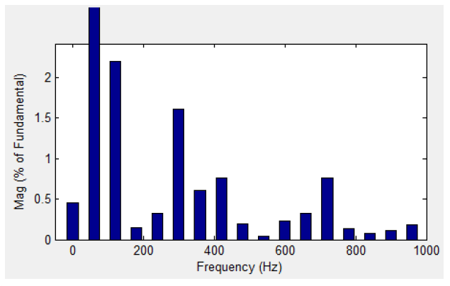
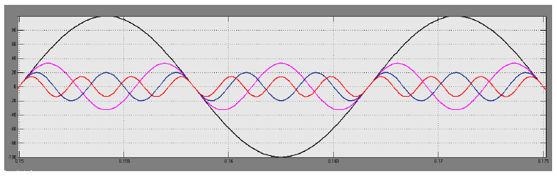
Where f_h is the h^th harmonic and f_ac is the fundamental frequency of system. Harmonics follow an inverse law in the sense that greater the harmonic level of a particular harmonic frequency, the lower is its amplitude as shown in Fig.1. Therefore, usually in power line harmonics higher order harmonics are not given much importance. The vital and the most troublesome harmonics are thus 3^rd, 5^th, 7^th, 9^th, 11^th and 13^th. The general expression of harmonics waveforms is given in eq. 2

V_n = V_msin(nωt) (2)

Where, V_m is the rms voltage of any particular frequency (harmonic or power line). The harmonics that are odd multiples of fundamental frequency are known as Odd harmonics and those that are even multiples of fundamental frequency are termed as Even harmonics. The frequencies that are in between the odd and even harmonics are called interharmonics.

Although, the ideal demand for any power utility is to have sinusoidal currents and voltages in AC system, this is not for all time promising, the currents and voltages with complex waveforms do occur in practice. Thus any complex waveform generated by such devices is a mixture of fundamental and the harmonics. Therefore, the voltage across a harmonically polluted system can be expressed numerically in eq. 3,

V = V_fpsin(ωt + ϕ₁) + V_2psin(2ωt + ϕ₂) + V_3psin(3ωt + ϕ₃) + V_npsin(nωt + ϕ_n) (3)

Where,
V_fp = Peak value of the fundamental frequency
V_np= Peak value of the nth harmonic component
ϕ = Angle of the respected frequency

Figure 1. Fundamental and harmonics frequency waveforms

Similarly, the expression for current through a given circuit in a harmonically polluted system is given by the expression given in eq. 4

I = I_fpsin(ωt + ϕ₁) + I_2psin(2ωt + ϕ₂) + I_3psin(3ωt + ϕ₃) ……+ I_npsin(nωt + ϕ_n) (4)

Harmonic components are also termed as positive, negative and zero sequence. In this case the harmonics that changes with the fundamental are called positive and those that have phasor direction opposite with the fundamental are called negative sequence components. The zero components do not take any affect from the fundamental and is considered neutral in its behavior. Phasor direction is pretty much important in case of motors. Positive sequence component tends to drive the motor in proper direction. Whereas the negative sequence component decreases the useful torque. The 7^th, 13^th, 19^th etc. are positive sequence components. The negative sequence components are 5^th, 11^th, 17^th and so on. The zero component harmonics are 3^rd, 9^th, 15^th etc. As the amplitude of harmonics decreases with the increase in harmonic order therefore, in power systems the utilities are more concerned about the harmonics up to 11^th order only.

3. Harmonics generation

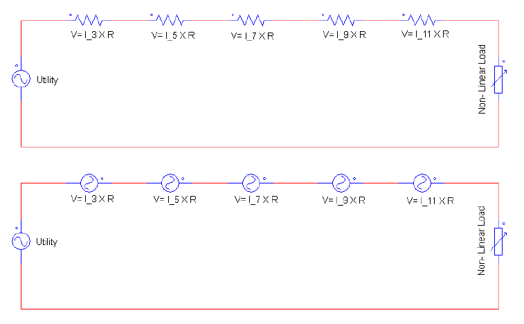
In most of the cases the harmonics in voltage is a direct product of current harmonics. Therefore, the current harmonics is the actual cause of harmonics generation. Power line harmonics are generated when a load draws a non-linear current from a sinusoidal voltage. Nowadays all computers use Switch Mode Power Supplies (SMPS) that convert utility AC voltage to regulate low voltage DC for internal electronics. These power supplies have higher efficiency as compared to linear power supplies and have some other advantages too. But being based on switching principle, these non-linear power supplies draw current in high amplitude short pulses. These pulses are rich in harmonics and produce voltage drop across system impedance. Thus, it creates many small voltage sources in series with the main AC source as shown in Fig.2. Here in Fig.2 I₃ refers to the third harmonic component of the current drawn by the non-linear load, I₅ is the fifth harmonic component of the load current and so on. R shows the distributed resistance of the line and the voltage sources are shown to elaborate the factor explained above. Therefore, these short current pulses create significant distortion in the electrical current and voltage wave shape. This distortion in shape is referred as a harmonic distortion and its measurement is carried out in term of Total Harmonic Distortion (THD). This distortion travels back into the power source and can affect other equipment connected to the same source. Any SMPS equipment installed anywhere in the system have an inherent property to generate continuous distortion of the power source that puts an extra load on the utility system and the components installed in it. Harmonics are also produced by electric drives and DC-DC converters installed in industrial setups. Uninterrupted Power Supply (UPS) and Compact Fluorescent Lamp (CFL) are also a prominent source of harmonics in a system. Usually high odd harmonics results from a power electronics converter. In summary, the harmonics are produced in an electrical network by [2, 16, 26, 42]

• Rectifiers
• Use of iron core in power transformers
• Welding equipment
• Variable speed drives
• Periodic switching of voltage and currents
• AC generators by non-sinusoidal air gap, flux distribution or tooth ripple
• Switching devices like SMPS, UPS and CFL

It is worth mentioning here that voltage harmonics can emerge directly due to an AC generator, due to a non-sinusoidal air gap, flux distribution, or to tooth ripple, which is caused by the effect of the slots, which house the windings. In large supply systems, the greatest care is taken to ensure a sinusoidal output from the generator, but even in this case any non-linearity in the circuit will give rise to harmonics in the current waveform. Harmonics can also be generated due to the iron cores in the transformers. Such transformer cores have a non-linear B-H curve [37].

Figure 2. Voltage distortion due to non-linear current

4. Problems associated with harmonics

Harmonically polluted system has many threats for its stability. It not only hampers the power quality (PQ) but when a current is rich in harmonics, is drawn by some device, it overloads the system. For example third harmonic current has a property that unlike other harmonic component it adds up into the neutral wire of the system. This results in false tripping of circuit breaker. It also affects the insulation of the neutral cable. Overloading of the cables due to harmonically polluted current increases the losses associated with the wires. It should also be kept in mind that only the power from fundamental component is the useful power, rest all are losses. These additional losses make the power factor poor that results in more power losses. The overall summarized effects of harmonics in the power system include the following [9, 18, 39]

• Harmonic frequencies can cause resonant condition when combined with power factor correction capacitors
• Increased losses in system elements including transformers and generating plants
• Ageing of insulation
• Interruption in communication system
• False tripping of circuit breakers
• Large currents in neutral wires

The distribution transformers have a Δ-Y connection. In case of a highly third harmonic current the current that is trapped in the neutral conductor creates heat that increases the heat inside the transformer. This may lead to the reduced life and de-rating of transformer. The different types of harmonic have their own impact on power system. For instance let us consider the 3^rd harmonic. Contrary to the balanced three phase system where the sum of all the three phases is zero in a neutral system, the third harmonic of all the three phases is identical. So it adds up in the neutral wire. The same is applicable on triple-n harmonics (odd multiples of 3 times the fundamental like 9^th, 15^th etc.). These harmonic currents are the main cause of false tripping and failure of earth fault protection relay. They also produce heat in the neutral wire thus a system needs a thicker neutral wire if it has third harmonic pollution in it. If a motor is supplied a voltage waveform with third harmonic content in it, it will only develop additional losses, as the useful power comes only from the fundamental component.

5. Harmonics monitoring standards

The identification of harmonics as a problem in AC power networks, has forced the utilities and regulatory authorities to devise the standards for harmonics monitoring and evaluation. The standards for harmonic control thus address both the consumers and the utility. Therefore, if the customer is not abiding by the regulations and is creating voltage distortion at the point of common coupling the utility can penalize him/her. Various renowned engineering institutes like IEEE, IEC and IET have devised laws to limit the injection of harmonic content in the grid. These standards are mostly helpful to achieve a user friendly healthy power quality system. IEEE standards are widely cited for their capability to address all the regions in the world. There are more than 1000 IEEE standards on electrical engineering fields. IEEE standards on power quality, however, are our main inspiration here. IEEE standard on harmonic control in electrical power system was published in 1992 and it covers all aspects related to harmonics [7]. It defines the maximum harmonics distortion up to 5 % on voltage levels ≤ 69kV. However, as the voltage levels are increased the allowable limits for harmonics in this standard are decreased to 1.5 % on all voltages ≥ 161 kV. It is also worth mentioning that individual voltage distortion starts from 3 % and ends at 1.0 % for voltage levels of ≤ 69kV and ≥ 161 kV respectively. Besides the standards that are designed keeping in view the global requirements, regional authorities devise their own standards according to their load profile and climatic conditions. Most of the standards are made according to the regional requirements of the country whereas few are based on the global needs and requirements. In Saudi Arabia there exists a regulatory body that defines the permissible limits and standard operational procedures for electricity transmission, distribution and generation. This body is known as electricity and cogeneration regulatory authority [38]. Apart from devising standards they also follow some standards defined by UAE power distribution companies. One such standard defined by Saudi Electric Company (SEC) in 2007 and is known as “Saudi Grid Code”. Harmonics limit set by the Saudi authorities is almost the same as IEEE standard but with a bit flexible limit of 3% THD for all networks operating within the range of 22kV-400kV [35, 38]. Table 1 compares the IEEE standard, the Abu Dhabi distribution company and the SEC standard for the harmonics limit in the electric network. It is interesting to mention that IEEE standard for controlling harmonics is silent for the conditions where a system is polluted with interharmonics (non-integer frequencies of fundamental frequency). For such conditions power utilities use IEC standard number 61000-2-2 .The IEC also defines the categories for different electronic devices in standard number 61000-3-2. These devices are then subjected to different allowable limits of THD. For example, class A has all three phase balanced equipment, non-portable tools, audio equipment, dimmers for only incandescent lamp. The limit for class A is varied according to the harmonic order. So for devices of class A the maximum allowable harmonic current is 1.08 A for 2^nd, 2.3A for 3^rd, 0.43A for 4^th, 1.14A for 5^th harmonics. The beauty of this IEC standard is that it also caters for power factor. For example all devices of class C (lighting equipment other than the incandescent lamp dimmer) have 3^rd harmonic current limit as a function of circuit power factor.

Table 1. Comparison of Harmonic Standards [7, 35, 38]

	SEC Standard	Abu Dhabi Distribution Company	IEEE Limits
Harmonics	THD limit is 5% for 400 V system, and 4% and 3% for 6.6- 20kV and 22kV- 400kV respectively	THD limit is 5% for 400 V system, and 4% and 3% for 6.6- 20kV and 22kV-400kV respectively	5% for all voltage levels below 69kV and 3% for all voltages above 161 kV

The modern systems based on artificial intelligent techniques like Fuzzy logic, ANFIS and CI based computations are reducing the difficulty of data mining that helps in redesigning the standards for power quality harmonics [24, 25]. In developed countries like Australia, Canada, USA the power distribution companies are already partially shifted to smart grid and they are using sophisticated sensors and measuring instruments. In terms of smart grid environment these sensors will help in mitigating the problems by predicting them in advance. Smart grid, by taking intelligent measurements and by the aid of sophisticated algorithms will be able to predict the PQ problems like harmonics, fault current in advance. It is pertinent to mention that the power quality monitoring using the on-going 3G technologies has been implemented by Chinese researchers. They used module of GPRS that is capable of analyzing the real time data and its algorithm makes it intelligent enough to get the desired PQ information [22].

6. Harmonics measurement

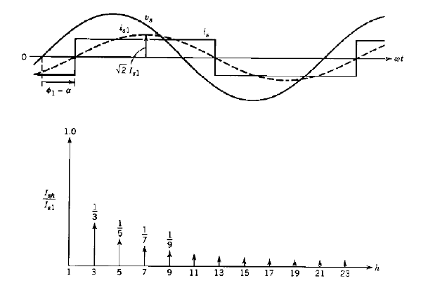
The real challenge in a harmonically polluted environment is to understand and designate the best point for measuring the harmonics. Nowadays the revolution in electronics has messed up the AC system so much that almost every user in a utility is a contributor to the harmonics current. Furthermore, the load profile in any domestic area varies from hour to hour within a day. So in order to cope with the energy demand and to improve the power factor, utilities need to switch on and off the power factor correction capacitors. This periodic and non-uniform switching also creates harmonics in the system. The load information in an area although, provide some basic information about the order of harmonic present in a system. Such information is very useful as it gives a bird eye view of harmonic content. But for the exact identification of the harmonics it is necessary to synthesize the distorted waveform using the power quality analyzer or using some digital oscilloscope for Fast Fourier Transform (FFT). For example Fig.3 shows a general synthesis of the current drawn by a controlled rectifier. Once identified, the level and type of harmonics (3^rd, 5^th etc.) the steps to mitigation can be devised. It should be kept in mind that proper measurement is the key for the proper designing of harmonic filters. But the harmonics level may differ at different points of measurement in a system. Therefore, utilities need to be very precise in identifying the correct point for harmonic measurement in a system. Among the standards, it is IEEE standard 519-1992 that outlines the operational procedures for carrying out the harmonic measurements. This standard however does not state any restriction regarding the integration duration of the measurement equipment with the system. It however, restricts the utility to maintain a log for monthly records of maximum demand [5]. Various devices are used in support with each other to carry out the harmonic measurements in a system. These include the following

• Power Quality Analyser
• Instrument transformers based transducers (CT and PT)

Figure 3. Typical line current of a controlled converter [26]

Various renowned companies are designing and producing excellent PQ analyzers. These include FLUKE, AEMC, HIOKI, DRANETZ and ELSPEC. These companies design single phase and three phase PQ analyzers that are capable of measuring all the dominant harmonic frequencies. The equipment that is used for harmonic measurement is also bound to some limitations for proper harmonic measurement. This limitation is technical in nature as for accurate measurement of all harmonic currents below the 65^th harmonic, the sampling frequency should be at least twice the desired input bandwidth or 8k samples per second in this case, to cover 50Hz and 60Hz systems [5]. Mostly, the PQ analyzers are supplied along with the CT based probes but depending on the voltage and current ratings a designer can choose the CT and PT with wide operating frequency range and low distortion. The distance of equipment with the transducer is also very important in measuring harmonics. If the distance is long then noise can affect the measurement therefore properly shielded cables like coaxial cable or fiber optic cables are highly recommended by the experts [5]. In short, the measurement of harmonics should be made on Point of Common Coupling (PCC) or at the point where non-linear load is attached. This includes industrial sites in special as they are the core contributors in injecting harmonic currents in the system.

7. Harmonics purging techniques

Techniques have been designed and tested to tackle this power quality issue since the problem is identified by the researchers. There are several techniques in the literature that addresses the mitigation of harmonics. All these techniques can be classified under the umbrella of following

i. Passive harmonic filter
ii. Active harmonic filter
iii. Hybrid harmonic filter
iv. Switching techniques

7.1. Passive harmonic filters

Passive filter techniques are among the oldest and perhaps the most widely used techniques for filtering the power line harmonics. Besides the harmonics reduction passive filters can be used for the optimization of apparent power in a power network. They are made of passive elements like resistors, capacitors and inductors. Use of such filters needs large capacitors and inductors thus making the overall filter heavier in weight and expensive in cost. These filters are fixed and once installed they become part of the network and they need to be redesigned to get different filtering frequencies. They are considered best for three phase four wire network [18]. They are mostly the low pass filter that is tuned to desired frequencies. Giacoletto and Park presented an analysis on reducing the line current harmonics due to personal computer power supplies [10]. Their work suggested that the use of such filters is good for harmonics reduction but this will increase the reactive component of line current. Various kind of passive filter techniques are given below [18, 19].

i. Series passive filters
ii. Shunt passive filters
iii. Low pass filters or line LC trap filters
iv. Phase shifting transformers

7.1.1. Series passive filters

Series passive filters are kinds of passive filters that have a parallel LC filter in series with the supply and the load. Series passive filter shown in Fig.4 are considered good for single phase applications and specially to mitigate the third harmonics. However, they can be tuned to other frequencies also. They do not produce resonance and offer high impedance to the frequencies they are tuned to. These filters must be designed such that they can carry full load current. These filters are maintenance free and can be designed to significantly high power values up to MVARs [4]. Comparing to the solutions that employ rotating parts like synchronous condensers they need lesser maintenance.

7.1.2. Shunt passive filters

These type of filters are also based on passive elements and offer good results for filtering out odd harmonics especially the 3^rd, 5^th and 7^th. Some researchers have named them as single tuned filters, second order damped filters and C type damped filters [3]. As all these filters come in shunt with the line they fall under the cover of shunt passive filters, as shown in Fig.5. Increasing the order of harmonics makes the filter more efficient in working but it reduces the ease in designing. They provide low impedance to the frequencies they are tuned for. Since they are connected in shunt therefore they are designed to carry only harmonic current [18]. Their nature of being in shunt makes them a load itself to the supply side and can carry 30-50% load current if they are feeding a set of electric drives [13]. Economic aspects reveal that shunt filters are always economical than the series filters due to the fact that they need to be designed only on the harmonic currents. Therefore they need comparatively smaller size of L and C, thereby reducing the cost. Furthermore, they are not designed with respect to the rated voltage, thus makes the components lesser costly than the series filters [33]. However, these types of filters can create resonant conditions in the circuit.

Figure 5. Different order type shunt filters [3]

7.1.3. Low pass filter

Low pass filters are widely used for mitigation of all type of harmonic frequencies above the threshold frequency. They can be used only on nonlinear loads. They do not pose any threats to the system by creating resonant conditions. They improve power factor but they must be designed such that they are capable of carrying full load current. Some researchers have referred them as line LC trap filters [19]. These filters block the unwanted harmonics and allow a certain range of frequencies to pass. However, very fine designing is required as far as the cut off frequency is concerned.

7.1.4. Phase shifting transformers

The nasty harmonics in power system are mostly odd harmonics. One way to block them is to use phase shifting transformers. It takes harmonics of same kind from several sources in a network and shifts them alternately to 180° degrees and then combine them thus resulting in cancelation. We have classified them under passive filters as transformer resembles an inductive network. The use of phase shifting transformers has produced considerable success in suppressing harmonics in multilevel hybrid converters [34]. S. H. H. Sadeghi et.al. designed an algorithm that based on the harmonic profile incorporates the phase shift of transformers in large industrial setups like steel industry [36].

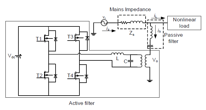
7.2. Active harmonic filters

In an Active Power Filter (APF) we use power electronics to introduce current components to remove harmonic distortions produced by the non-linear load. Figure 6 shows the basic concept of an active filter [27]. They detect the harmonic components in the line and then produce and inject an inverting signal of the detected wave in the system [27]. The two driving forces in research of APF are the control algorithm for current and load current analysis method [23]. Active harmonic filters are mostly used for low-voltage networks due to the limitation posed by the required rating on power converter [21].

Figure 6. Conceptual demonstration of Active filter [27]

They are used even in aircraft power system for harmonic elimination [6]. Same like passive filters they are classified with respect to the connection method and are given below [40].

i. Series active filters
ii. Shunt active filters

Since, it uses power electronic based components therefore in literature a lot of work has been done on the control of active filters.

7.2.1. Series active filter

The series filter is connected in series with the ac distribution network as show in Fig.7 [33]. It serves to offset harmonic distortions caused by the load as well as that present in the AC system. These types of active filters are connected in series with load using a matching transformer. They inject voltage as a component and can be regarded as a controlled voltage source [33]. The drawback is that they only cater for voltage harmonics and in case of short circuit at load the matching transformer has to bear it [31].

7.2.2. Shunt active filter

The parallel filter is connected in parallel with the AC distribution network. Parallel filters are also known as shunt filters and offset the harmonic distortions caused by the non linear load. They work on the same principal of active filters but they are connected in parallel as stated that is they act as a current source in parallel with load [21]. They use high computational capabilities to detect the harmonics in line.

Mostly microprocessor or micro-controller based sensors are used to estimate harmonic contents and to decide the control logic. Power semiconductor devices are used especially the IGBT. Some researchers claim that before the advent of IGBTs active filters were seldom use due to overshoot in budget [11]. However, despite of their usefulness shunt active filters have many drawbacks. Practically they need a large rated PWM inverter with quick response against system parameters changes. If the system has passive filters attached somewhere, as in case of hybrid filters then the injected currents may circulate in them [28].

7.3. Hybrid harmonic filters

These types of filters combine the passive and active filters. They contain the advantages of active filters and lack the disadvantages of passive and active filters. They use low cost high power passive filters to reduce the cost of power converters in active filters that is why they are now very much popular in industry. Hybrid filters are immune to the system impedance, thus harmonic compensation is done in an efficient manner and they do not produce the resonance with system impedance [29]. The control techniques used for these types of filters are based on instantaneous control, on p-q theory and i_d-i_q. K.N.M.Hasan et.al. presented a comparative study among the p-q and i_d-i_q techniques and concluded that in case of voltage distortions the i_d-i_q method provides slightly better results [12]. They are usually combined in the following ways [21]

i. Passive series active series hybrid filters
ii. Passive series active shunt hybrid filters
iii. Passive shunt active series hybrid filters
iv. Passive shunt active shunt hybrid filters

7.3.1. Passive series active series hybrid filters

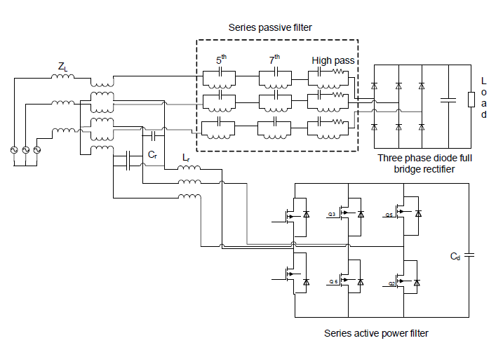
These type of hybrid filters have both kind of filters connected in series with the load as shown in Fig.8 and are considered good for diode rectifiers feeding a capacitive load [32]

7.3.2. Passive series active shunt hybrid filters

This breed of hybrid filter has passive part in series with load and active filter in parallel. AdilM. Al-Zamil et al. proposed such type of filters in their paper and used the high power capability. of passive filter by placing them in series with the load. They used an active filter with space vector pulse with modulation (SVPWM) and implemented it on micro-controller. They used only line current sensors to compute all the parameters required for reference current generation. Their proposed system worked satisfactorily up to the 33^rd harmonic and the results shown are based on a system with line reactance of 0.13 pu. In their system the bandwidth required for active filter is relatively less due to the passive filter that takes care of the rising and falling edges of load current. They proposed that while designing hybrid system the line filter L and capacitance C of active filter needs a compromise in selection depending on the acceptable level of switching frequency ripple current and minimum acceptable ripple voltage [1].

7.3.3. Passive shunt active shunt hybrid filters

These types of filters have both the passive and active filters connected in shunt with the load as shown in Fig.9 [21]. In a comparative study J.Turunen et al. claimed that they require smallest transformation ratio of coupling transformer as a result they need a fairly high power rating for a small load and in case of high power loads the problem of dc link control results in poor current filtering [43].

7.3.4. Passive shunt active series hybrid filters

As its name implies it is a kind of hybrid filter that has an active filter in series and a passive filter in shunt as shown in Fig.10. J. Turunen et al. in a comparative study stated that this breed of hybrid filter utilizes very small transformation ratio therefore for same rating of load their power rating required is large compared to the load [43].

Figure 8. Passive series active series hybrid filters [32]

Figure 9. Passive shunt active shunt hybrid filters [21]

Figure 10. Active series passive shunt hybrid filters [29]

7.4. Switching techniques

Besides using the method of installing filters, power electronics is so versatile that up to some extent harmonics can be eliminated using switching techniques. These techniques may vary from the increasing the pulse number to advance algorithm based Pulse Width Modulation (PWM). The most widely used sine triangle PWM was proposed in 1964. Later in 1982 Space Vector PWM (SVPWM) was proposed [20]. PWM is a magical technique of switching that gives unique results by varying the associated parameters like modulation index, switching frequency and the modulation ratio. The frequency modulation ratio ‘m’ if taken as odd automatically removes even harmonics [17, 26]. Here the increase in switching frequency reduces the current harmonics but this makes the switching losses too much. Furthermore, we cannot keep on increasing switching frequency because this imposes the EMC problems [15]. D.G.Holmes et al. presented an analysis for carrier based PWM and claimed that it is possible to use some analytical solutions to pin point the harmonic cancelation using different modulation techniques. Sideband harmonics can be eliminated if the designer uses natural or asymmetric regular sampled PWM [14]. The output can be improved by playing with the modulation index. One specialized type of PWM is called Selective Harmonic Elimination (SHE) PWM or the programmed harmonic elimination scheme. This technique is based on Fourier analysis of phase to ground voltage. It is basically a combination of square wave switching and the PWM. Here proper switching angles selection makes the target harmonic component zero [26, 30]. In SHE technique a minimum of 0.5 modulation index is possible [41]. But even the best SHE left the system with some unfiltered harmonics. J. Pontt et al. presented a technique of treating the unfiltered harmonics due to the SHE PWM. They stated that if we use SHE PWM for elimination of 11^th and 13^th harmonics for 12 pulse configuration then the harmonics of order 23^th, 25^th, 35^th and 37^th are one that play vital role in defining the voltage distortions. They proposed the use of three level active front end converters. They suggested a modulation index of 0.8-0.98 to mitigate the harmonics of order 23^rd, 25^th and 35^th, 37^th [30]. With some modifications researchers have shown that SHE PWM can be used at very low switching frequency of 350 Hz. Javier Napoles et al. presented this technique and give it a new name of Selective Harmonic Mitigation (SHM) PWM. They used seven switching states and results makes the selective harmonics equal to zero [8]. This is excellent since in SHE PWM the selective harmonic need not to be zero. It is sufficient in conventional PWM to bring it under the allowable limit. Siriroj Sirisukprasert et al. presented an optimal harmonic reduction technique by varying the nature of output stepped waveforms and varied the modulation indexes. They tested their proposed technique on multilevel inverters that are better than the two level conventional inverters. They excluded the very narrow and very wide pulses from the switching waveform. Unlike SHE PWM as discussed above they ensured the minimum turn on and turn off by switching their power switches only once a cycle. Contrary to traditional SHE PWM, in this case the modulation index can vary till 0.1. The output is a stepped waveform for different stages they classify the production of modulation index as high, low and medium and the real point of interest is that for all these three classes of modulation indexes the switching is once per cycle per switch [41]. Some researchers used trapezoidal PWM method for harmonic control. This kind of PWM is based on unipolar PWM switching. Here a trapezoidal waveform is compared with a triangular waveform and the resulting PWM is supplied to the power switches. Like other harmonic elimination techniques in PWM based techniques researchers have proposed the use of AI based techniques including FL and ANN.

8. Conclusion

This chapter summarizes one of the major power quality problems that is the reason of many power system disturbances in an electrical network. The possible sources of harmonics are discussed along with their effects on distribution system components including the transformers, switch gears and the protection system. The regulatory standards for the limitation of harmonics and their measurement techniques are also presented here. The purging techniques of harmonics are also presented and various kind of harmonic filters are briefly presented. To strengthen the knowledge base, this chapter has also discussed the control of harmonics using PWM techniques. By this chapter we have attempted to gather the technical information in this field. A thorough understanding of harmonics will provide the utility engineers a framework that is often required in the solution of research work related to harmonics.

Author details
Hadeed Ahmed Sher* and Khaled E Addoweesh
Department of Electrical Engineering, King Saud University, Riyadh, Saudi Arabia

Yasin Khan
Department of Electrical Engineering, King Saud University, Riyadh, Saudi Arabia Saudi Aramco Chair in Electrical Power, Department of Electrical Engineering, King Saud University, Riyadh

9. References

[1] A.M. Al-Zamil and D.A. Torrey. “A passive series, active shunt filters for high power applications”. Power Electronics, IEEE Transactions on, 16(1):101–109, 2001.
[2] S.J.Chapman. “Electric machinery fundamentals”. McGraw-Hill Science/ Engineering/Math, 2005.
[3] C.J. Chou, C.W. Liu, J.Y. Lee, and K.D. Lee. “Optimal planning of large passiveharmonic filters set at high voltage level”. Power System IEEE Transactions on, 15(1):433–441, 2000.
[4] JC Das. “Passive filters-potentialities and limitations”. In Pulp and Paper Industry Technical Conference, 2003. Conference Record of the 2003 Annual, pages 187–197. IEEE, 2003.
[5] F. De la Rosa and Engnetbase. “Harmonics and power systems”. Taylor&Francis, 2006.
[6] A. Eid, M. Abdel-Salam, H. El-Kishky, and T. El-Mohandes. “Active power filters for harmonic cancellation in conventional and advanced aircraft electric power systems.” Electric Power Systems Research, 79(1):80–88, 2009.
[7] I. F II. “IEEE recommended practices and requirements for harmonic control in electrical power systems”. 1993.
[8] L.G. Franquelo, J. Napoles, R.C.P. Guisado, J.I. Leon, and M.A. Aguirre. “A flexible selective harmonic mitigation technique to meet grid codes in three-level PWM converters”. Industrial Electronics, IEEE Transactions on, 54(6):3022–3029, 2007.
[9] E.F. Fuchs and M.A.S. Masoum. “Power quality in power systems and electrical machines” .Academic Press, 2008.
[10] LJ Giacoletto and GL Park. “Harmonic filtering in power applications”. In Industrial and Commercial Power Systems Technical Conference, 1989, Conference Record., pages 123–128. IEEE, 1989.
[11] C.A. Gougler and JR Johnson. “Parallel active harmonic filters: economical viable technology”. In Power Engineering Society 1999 Winter Meeting, IEEE, volume 2, pages 1142–1146. IEEE.
[12] K.N.M. Hasan and M.F. Romlie. “Comparative study on combined series active and shunt passive power filter using two different control methods”. In Intelligent and Advanced Systems, 2007. ICIAS 2007. International Conference on, pages 928–933. IEEE, 2007.
[13] F.L. Hoadley. “Curb the disturbance”. Industry Applications Magazine, IEEE, 14(5):25–33,2008.
[14] D.G. Holmes and B.P. McGrath. “Opportunities for harmonic cancellation with carrier-based PWM for a two-level and multilevel cascaded inverters.” Industry Applications, IEEE Transactions on, 37(2):574–582, 2001.
[15] J. Holtz. “Pulse width modulation-A survey.” Industrial Electronics, IEEE Transactions on, 39(5):410–420, 1992.
[16] H.Rashid. “Power Electronics Circutis Devices and Applications”. Prentice Hall Int. Ed.,1993.
[17] I.B. Huang and W.S. Lin. “Harmonic reduction in inverters by use of sinusoidal pulsewidth modulation.” Industrial Electronics and Control Instrumentation, IEEE Transactions on, (3):201–207, 1980.
[18] J. David Irwin. “The industrial electronics handbook”. CRC, 1997.
[19] D. Kampen, N. Parspour, U. Probst, and U. Thiel. “Comparative evaluation of passive harmonic mitigating techniques for six pulse rectifiers” In Optimization of Electrical and Electronic Equipment, 2008. OPTIM 2008. 11th International Conference on, pages 219–225. IEEE, 2008.
[20] M.P. Ka´zmierkowski and R. Krishnan. “Control in power electronics: selected problems.” Academic Pr, 2002.
[21] B.R. Lin, B.R. Yang, and H.R. Tsai. “Analysis and operation of hybrid active filter for harmonic elimination”. Electric Power Systems Research, 62(3):191–200, 2002.
[22] D. LU, H. ZHANG, and C. WANG. “Research on the reliable data transfer based on udp” [j]. Computer Engineering, 22, 2003.
[23] L. Marconi, F. Ronchi, and A. Tilli. “Robust nonlinear control of shunt active filters for harmonic current compensation”. Automatica, 43(2):252–263, 2007.
[24] W.G. Morsi and ME El-Hawary. “A new fuzzy-based representative quality power factor for unbalanced three-phase systems with non-sinusoidal situations” Power Delivery, IEEE Transactions on, 23(4):2426–2438, 2008.
[25] S. Nath and P. Sinha. “Measurement of power quality under non-sinusoidal condition using wavelet and fuzzy logic”. In Power Systems, 2009. ICPS’09. International Conference on, pages 1–6. IEEE,2009.
[26] N. Mohan,T. Undeland and W. P. Robbins. “Power Electronics Converters, Applications and Design” Wiley India, 2006.
[27] N. Pecharanin, M. Sone, and H. Mitsui. “An application of neural network for harmonic detection in active filter”. In Neural Networks, 1994. IEEE World Congress on Computational Intelligence., 1994 IEEE International Conference on, volume 6, pages 3756–3760. IEEE, 1994.
[28] F.Z. Peng, H. Akagi, and A. Nabae. “A new approach to harmonic compensation in power systems-a combined system of shunt passive and series active filters”. Industry Applications, IEEE Transactions on, 26(6):983–990, 1990.
[29] F.Z. Peng, H. Akagi, and A. Nabae. “Compensation characteristics of the combined system of shunt passive and series active filters”. Industry Applications, IEEE Transactions on, 29(1):144–152, 1993.
[30] J. Pontt, J. Rodriguez, R. Huerta, and J. Pavez. “A mitigation method for non-eliminated harmonics of SHE PWM three-level multipulse three-phase active front end converter.” In Industrial Electronics, 2003. ISIE’03. 2003 IEEE International Symposium on, volume 1, pages 258–263. IEEE, 2003.
[31] NA Rahim, S. Mekhilef, and I. Zahrul. “A single-phase active power filter for harmonic compensation”. In Industrial Technology, 2005. ICIT 2005. IEEE International Conference on, pages 1075–1079. IEEE, 2005.
[32] S. Rahmani, K. Al-Haddad, and F. Fnaiech. “A hybrid structure of series active and passive filters to achieving power quality criteria”. In Systems, Man and Cybernetics, 2002 IEEE International Conference on, volume 3, pages 6–pp. IEEE, 2002.
[33] M.H. Rashid. “Power electronics handbook”. Academic Pr, 2001.
[34] C. Rech and JR Pinheiro. “Line current harmonics reduction in hybrid multilevel converters using phase-shifting transformers”. In Power Electronics Specialists Conference, 2004. PESC04. 2004 IEEE 35th Annual, volume 4, pages 2565–2571. IEEE, 2004.
[35] Regulation, supervision bureau for the water, and electricity sector of the Emirate of Abu Dhabi. “Limits for harmonics in the electricity supply system”. 2005.
[36] SHH Sadeghi, SM Kouhsari, and A. Der Minassians. “The effects of transformers phaseshifts on harmonic penetration calculation in a steel mill plant”. In Harmonics and Quality of Power, 2000. Proceedings. Ninth International Conference on, volume 3, pages 868–873. IEEE, 2000.
[37] C. Sankaran. “Power quality”. CRC, 2002.
[38] SEC. “The Saudi Arabian grid code”, 2007.
[39] J. Shepherd, A.H. Morton, and L.F. Spence. “Higher electrical engineering.” Pitman Pub.,1975.
[40] B. Singh, K. Al-Haddad, and A. Chandra. “A review of active filters for power quality improvement”. Industrial Electronics, IEEE Transactions on, 46(5):960–971, 1999.
[41] S. Sirisukprasert, J.S. Lai, and T.H. Liu. “Optimum harmonic reduction with a wide range of modulation indexes for multilevel converters”. Industrial Electronics, IEEE Transactions on, 49(4):875–881, 2002.
[42] W. Theodore et al. “Electrical Machines, Drives And Power Systems” 6/E. Pearson Education India, 2007.
[43] J. Turunen, M. Salo, and H. Tuusa. “Comparison of three series hybrid active power filter topologies” In Harmonics and Quality of Power, 2004. 11th International Conference on, pages 324–329. IEEE, 2004.

Source: https://www.intechopen.com/chapters/43901

Industrial Grids with Frequency Inverters and Localization of the Earth Fault

Published by Tomáš SNIEGOŇ, Jiří GURECKY,
Department of Electrical Power Engineering, VŠB – TU Ostrava

Abstract. This article focuses on industrial grids with frequency inverters and evaluation of the earth fault and its localization. In the first part the system of localization of the earth fault, industrial grids with frequency inverters and typical application in industry are described. The feedback effect of frequency inverters on the supply network is specified too. The second part of the article aims at the description of practical measuring of the earth fault on the testing panel. The third part deals with the summary of measuring and that of the experience with industrial grids and localization of the earth fault. The summary is included in the last part as well.

Streszczenie. Artykuł ten przedstawia sieci przemysłowe z falownikami i lokalizację doziemienia w sieci z izolowanym punktem neutralnym. W pierwszej części opisany jest system lokalizacyjny doziemienia, sieci przemysłowe z falownikami i typowa aplikacja w przemyśle. Przedstawiono również wpływ falowników na sieć zasilającą. Druga część artykułu dotyczy opisu zrealizowanych pomiarów doziemień z wykorzystaniem panelu testowego. W trzeciej części streszczono pomiary, przedstawiono doświadczenia wynikające z pracy z sieciami przemysłowymi i z systemem lokalizacji doziemienia. (Sieci przemysłowe z falownikami I lokalizacją doziemienia)

Keywords: industrial grids, frequency inverters, earth fault, isolated neutral system IT, earth fault localization.
Słowa kluczowe: sieci przemysłowe, falowniki, doziemienie, sieć o izolowanym punkcie neutralnym IT, lokalizacja doziemień

Introduction

Industrial grids are re-deformed by used devices (for example frequency inverters and others). There are devices sensitive to the quality of the mains too. The earth fault causes a large overvoltage. Therefore the earth fault should be monitored .The speed of evaluation of the earth fault can influence correction of errors and thus can effect continuity of the production process. In the article the industrial grids with frequency inverters, the system of localization of the earth fault and several measurements made on the test network model will be described.

The earth fault in industrial conditions

The LV grid with isolated neutral system IT in industrial conditions undoubtedly has many benefits that contribute to the continuity of the production process and to the minimization of the power system failure. On the other hand, in practice the negative effects associated with the operation of these networks also have to be solved. In this article the attention is focused on the problems caused by earth faults and on the question how to localize the earth fault in the shortest possible time. Nowadays, the protection systems of the insulated conditions are used. The protector is able to evaluate both the earth fault and the worsened state of insulation. At the same time the outcome of the evaluation is signaled in the control room with the permanent service. If the network is not too extensive, the operation and manufacturing process enables to disconnect the terminals. Otherwise, there is a problem to find the place of the failure.

The earth fault in the IT grid

In the isolated networks, under the conductive connection of the one phase to the earth, the short-circuit will not happen but there will be so called earth fault. According to the size of the contact resistance in the place of earth fault, the following can be categorized:

a) Resistance earth fault – the value of the contact resistance is of the order of several hundreds of ohms
b) Metal and arc-earth fault – the value of the contact resistance is only a few ohms, usually negligible According to the duration of the mentioned states, the following can be classified:

a) Fast-acting earth fault – up to 0.5 seconds
b) Short-term earth fault – up to 5 minutes
c) Intermittent earth fault – fast-acting and short-term earth
fault repeated several times
d) Permanent earth connection – until its removal it usually takes several hours [1]

The duration of earth fault is an important parameter which has a major impact on the successful identification and localization of a failure condition. We can come across various modes of the electrical equipment operation, from the continuous operation of the fan and pump drives to the instantaneously switched drives, for example. According to the daily operation of the track, the drives of the rules appeared on the block stool reach about 20, 000 operating cycles per 24 hours. Identification and localization of the earth fault has to reflect these facts [3].

Industrial grids with frequency inverters

Nowadays, frequency inverters are used in many applications. This is caused by automation of production. Frequency inverters enable to change frequency and voltage, limit the current and others for better regulation of the drive. Inverters have a good power factor but harmonic distortion load the power system. High energy costs force companies to use regenerative converters in some applications. All this can affect the quality of the mains.

Typical application in the industry

Typical industrial applications are conveyers in rolling mills (see fig. 1). Frequency inverters are currently used on conveyors and many other devices. Frequency inverters load the power system by harmonic distortion. These factors have the effect on the evaluation and localization of the earth fault. DC link of frequency inverter has an influence on the assessment too. Times comparison of evaluation of the earth fault between invertors and standard devices is included in this article. Distortion of the mains can be observed in the picture below (fig. 2). On the other hand, the possibility of limiting current with frequency inverter reduces the distortion of the mains at the start and reverse of the drive. As depicted in the pictures below, the time of the drive operation is very short. The drive operates on the nominal values only few second. Distortion parameters of the grid and short operate time of the drive make working conditions difficult for localization devices of the earth fault. Waveform of the current, speed and frequency of the conveyor are shown in the picture (see fig. 3)

Fig.3. Waveform of the current, speed and frequency

Testing and measuring of the earth fault location system on the model

In order to more detail testing of the system, the test model was created. The test model enables to try different settings and configurations to evaluate whether the change has or has not the impact on the speed and on the accuracy of the earth fault evaluation. It would not be possible to try this type of testing with the real network without the significant intervention into the production process. In the measuring circuit there are four measuring transformers, one at the inlet and the other three at the outlets into the individual motors. These transformers are connected to a positioning device. In case the protector of the isolated state finds the fault, the localization system will start to evaluate the location of the fault [4].

For testing purpose the components below were used:

– Identification device: BENDER A-ISOMETER® IRDH575
– Localization devices: BENDER EDS490-D
– Measuring transformer: BENDER W60
– Transformer: T105 380/500V
– Contactor: EPM C25.11
– Frequency inverter: ABB ACS800-01-0004-5
– Motor M1: MEZ Mohelnice 4AP90S-4 1,1 kW
– Motor M2: SIEMENS 1LA7096-4AA11 1,5 kW
– Motor M3: SIEMENS 1LA7096-6AA10 1,1 kW

There have been many measurements and tests with the device IRDH575 and EDS460 which should have evaluated sensitivity, accuracy, reliability and speed of the identification and localization of the earth fault. As the description of all these tests would be too extensive the article will be focused on a few examples.

Test focused on the speed of evaluation of the earth fault and its localization

Earth fault was simulated on the drive switching by the frequency inverter, without added leakage capacity. Fifty measurements were carried out; the times were written into the tables and then statistically analyzed. For illustration the table of the outcomes of twenty measurements is included in this article (see table 1).

Table 1. Measured times of identification and earth fault localization

Measuring n.	IRDH [s]	EDS [s]
1.	18,6	33,4
2.	24,2	39,2
3.	6,6	33,2
4.	4,4	19,2
5.	5,2	20,2
6.	11,6	26,4
7.	23,4	38,2
8.	7,6	22,4
9.	5,6	27,8
10.	6,8	28,8
11.	7,2	22,4
12.	9,6	24,6
13.	19,6	34,4
14.	13,2	28,2
15.	12	32,6
16.	9,2	24,4
17.	3,4	18,2
18.	5,2	25,8
19.	8,6	29,2
20.	5,6	20,6

The test evaluating the effect of stray capacitance In this case the earth fault was simulated on the drive switched by the frequency inverter, under the condition of added stray capacitance into the circuit. For illustration the table with the results of twenty measurements is given in this article (see table 2). The value of the stray capacitance was set at 4 µF, which is the value that corresponds to the medium-large cable network. Value of the capacitance can be determined as mentioned below:

– By calculation of the capacity of individual cables [2]

where: C – capacitance, l – length, h – distance, r – radius, ε₀ – electric constant, ε_r – matter constant

– By measuring

To verify whether the value 4µF corresponds to the values in the real network, the measurements of the network were taken.

Table 2. Measured times of identification and earth fault localization with leakage capacitance

Measuring n.	IRDH [s]	EDS [s]
1.	13	29,8
2.	11	32
3.	16,2	37
4.	9,2	24
5.	9,8	24,8
6.	16,2	31,2
7.	15,5	30,2
8.	27	41,8
9.	24,8	39,8
10.	14	34,6
11.	18,8	39,4
12.	14,4	29,2
13.	10,8	25,8
14.	19,4	40,2
15.	8,6	23,4
16.	14,2	29,2
17.	30,2	45,2
18.	10	25
19.	12,8	27,8
20.	7	21,8

Results of the measurements and tests

In the following table, comparison and summarization of measuring with and without the leakage capacitance in the circuit can be found (see table 3,4). The leakage capacitance is an essential factor for speed of identification and localization of the earth fault.

For illustration the times of identification and localization of the earth fault with leakage capacitance is included in the graph below (see fig. 5). For comparison the times simulated on the drive switched by the power contactor and the frequency inverter are given. [5]

Table 3. Comparison of the measuring with frequency inverters

	Without cap.	Without cap.	With cap.	With cap.
	IRHD [s]	EDS [s]	IRHD [s]	EDS [s]
Average	10,5	26,9	14,8	31,4
Minimum	3,2	18,2	6,2	21
Maximum	24,2	41,4	30,2	46,6

Table 4. Comparison of measuring with the power contactor

	Without cap.	Without cap.	With cap.	With cap.
	IRHD [s]	EDS [s]	IRHD [s]	EDS [s]
Average	3,1	18,7	8,4	24,9
Minimum	2	13,8	2,4	18,2
Maximum	4,2	24,2	14,4	46,6

Fig.5. The graph describing time of the earth fault evaluation and its localization with leakage capacitance

Conclusion

In all cases the localization system of the earth fault evaluated and localized the earth fault properly. In no case the “false evaluation” was reached, it means that system would evaluate the earth fault which would not be activated. As we can see, times between the power contactor and the frequency inverter are different. Average times of frequency inverter are approximately 8 seconds longer. From fig.3 the conclusion can be drawn that operating times of some devices (the conveyor in this case) are short. That has the effect on evaluation of the earth fault. Therefore successive measurements with other localization systems are necessary. The results of the analysis will then be applied to a real-life industrial environment to order to verify them. It will be interesting to compare measurements on the testing panel and those in the real grid.

REFERENCES

[1] Trojánek Z., Hájek J., Kvasnica P., Přechodové jevy v elektrizačních soustavách. SNTL 1987
[2] Hofheinz W., Protective Measures with Insulation Monitoring. VDE Verlag 2006
[3] Sniegoň T., Gurecký J., „Negative effects of the earth fault in insolated neutral system IT/500V on rolling mill for rail plant.” Sborník konference EPE, VUT Brno, 2010, vol. 11., p. 173-176
[4] Sniegoň T., Gurecký J., „Identification and localization of the earth fault in insolated Neutral system IT/500V in industrial environment.” Sborník konference EPE, 2011
[5] Sniegoň T., Gurecký J., Messerschmidt M., „System of localization of the earth fault in 500V/IT grids in industry.” Sborník konference EPE, 2012

Authors: Ing. Tomáš Sniegoň, Třinecké železárny, a.s., TřinecStaré město, Průmyslová 1000, 73970 Třinec, E-mail: tomas.sniegon@trz.cz, Department of Electrical Power Engineering, VŠB TU Ostrava Doc.Dr.Ing.Jiří GureckýE-mail: jiri.gurecky@vsb.cz, Department of Electrical Power Engineering, VŠB – TU Ostrava

Source & Publisher Item Identifier: PRZEGLĄD ELEKTROTECHNICZNY, ISSN 0033-2097, R. 89 NR 5/2013

Research of the Fault Location Method of Distribution Network

Published by Yan LI¹, Yu GUO², Xiping WANG¹,
Electrical engineering department Hebei Engineering and Technical College (1), Langfang Yongqing supply Co.,Ltd. (2)

Abstract. The rough set theory is used to realize the automatic fault location method of the rural power distribution network. The decision table of the distribution network fault location is based on the fault complaints information. It is automatically formed by distribution network topology. Then the decision table is property reduced based on identifiable matrix. Finally improved value reduction method is used to form the fault diagnosis expert knowledge uniformly. Combined with the GIS platform, it designs the application program of the fault location and realizes the visual fault localization.

Streszczenie. W artykule zaproponowano wykorzystanie teorii zbiorów przybliżonych w tworzeniu metody lokalizacji awarii w sieci elektroenergetycznej na terenie wiejskim. Metoda bazuje na drzewie decyzyjnym, w którym zawiera informacja o zgłoszeniach awarii. Opracowany algorytm redukcji wielkości drzewa, w połączeniu z platformą Systemu Informacji Geograficznej (ang. Geographic Information System – GIS), pozwala na dokładne określenie miejsca awarii. (Badanie metody lokalizacji awarii w sieci elektroenergetycznej).

Keywords: distribution network; non-measurement and control area; fault location; rough set; GIS
Słowa kluczowe: sieć elektroenergetyczna, rejon trudno dostępny, lokalizacja awarii, zbiory przybliżone, GIS.

Introduction

As the development of electronic technology, communication technology and computer technology, Many cities and rural departments have begun to implement power distribution management system (DMS) project, combining with Supervisory Control And Data Acquisition (SCADA) and Geographic Information System (GIS), make comprehensive monitoring and management to the distribution network, and have achieved some results. By installing the feeder terminal unit on the switch of the post outdoor, to get the real-time data which reflect the status of the distribution network, and through the fault information to do the fault location. However, due to constraints of construction cost and complexity, we generally only construct the Distribution Automation System. in the loan-up and important area. In the distribution network, only main feeder and long-branch have the Feeder Terminal Unit (FTU) on column. In rural power grid even install the RTU only in the substation, and considerable part of distribution lines are belong to the non management and control area of distribution net, they can not gain the real-time date because they do not have the FTU on column, only rely on customer telephone complaints messages (TCM) to help locate the fault. Therefore, relying solely on SCADA systems to provide fault information to distribution network fault location is actually not entirely feasible[1]. Based on the above situation, this article tries to apply rough set theory (Rough Sets) [2] to the non management and control areas of rural power grid for fault location, With a strong fault tolerance of rough sets and do not provide any prior information outside the processing date set. First use the telephone fault report in user area as condition attribute set for the fault location, consider all possible fault conditions and establish decision table. And then realize the automation simplification of decision table and the simplification of attribute values, to extract diagnosis rules and form a new knowledge library.

Fault location algorithm design

Mathematical description of the algorithm: In the non-measurement and control areas of distribution network, the fault site is determined according to the large number of complaints information received from different regions, that is the fault site can be inferred from the complaint calls. Because of the subjective factors and knowledge level of the user, the some of complaint information does not present the occurrence, some even contain uncertainty elements or error factor, so the complaints information is only a rough set. It will be more suitable to mathematically describe the distribution network fault location. Rough set (RS) [3] theory is proposed by a Polish scholars- z.pawlak in 1982. It is a new mathematical tool to characterize the incomplete and uncertainty. Algorithm design: In connection with a given distribution network topology, first, the telephone repair region is conducted as the fault classification condition attributes, considering all of the possible fault conditions, simplify the original information, find an equivalent reduction of the original information , then find the smallest reduction to further simplify, extract the decision rules, reveal the inherent redundancy of fault repair information, achieve the distribution system fault locating rapidly and accurately. The formation of decision table and the key Simple step are shown in Fig.1.

Fig.1. The simplification flow chart of the decision table of distribution network fault

formation of decision table. In this network component S presents breakers drop switches, 11 totally. There are 10 power supply regions (T1-T10), 10 transformers (T). The fault occurred at the component S presents that the line containing S is fault, also if the fault occurred at T, it presents that the transformer T is fault. The decision table is formed according to the analysis of distribution network topology. First of all, get the records set of transformer substation from geographic database, obtain the entire distribution network topology in accordance with the topology analysis algorithm in the GIS system map algorithm using breadth-first algorithm starting the cycle from the first record[4]. A breaker of the substation is assumed as the power point, it only corresponds to one line. Searches down from the circuit breaker using topology analysis algorithm, get the along switch, terminal transformers and the corresponding power supply region, and code them. The map 2 shows the distribution network, code the switching with S1, S2, …, S11, transformer with T1, T2, …, T10, the power supply area with T1 zone, T2 zone, …, T10 Zone . Then search for the supply area line through all equipment components, the power supply area code is “1”, other supply area code “0”, thus the original fault decision table is formed in Table 1. “1” presents that the user dial the fault complaints telephone, “0” presents that the user does not dial.Fig.3 shows the dynamic coding process of distribution network.

Fig.3. Flow chart of dynamic coding process of distribution network.

Identification matrix is an important concept in rough set theory. It accommodates arbitrarily complex information in a matrix, without the affecting of the original system. Thus the analytical ability is improved greatly. The simplification of information system is started on identification matrix. S = (U, A) is an information system, U is discuss domain and U = ( x₁, x₂, …, x_n), A is condition attribute set, D is decision attribute a (x) records the value of x on a, C_ij presents the element in the i row and j column. Identification matrix can be defined as (i, j = 1, 2, 3, ⋯, n):

Three kinds of value consist of the elements of the identification matrix. If the decision attribute of two records are different and the conditions attribute are different, the element value shall be the property combination of different attribute values; If the decision attribute of two records are the same and the conditions attribute are the same, the element value shall be 0; If the decision attribute of two records are different but the conditions attribute are the same, the two record are conflict, the element value shall be -1.

The decision table is simplified according to the identification matrix, the following steps: (1) Change the decision table into identification matrix, find the kernel property which the property combination is 1 and property combination which does not contain kernel property. (2) The condition attribute set which does not contain kernel attribute expressed as ANF, and calculate, that is P=∧{Vbi,k(i=1,2,….,s;k=1,2,…,m)},change it into ANF, and simplify. (3) All ANF and kernel attribute compose of reduction set.

In order to remove redundant information in the decision table, the property value reduction is introduced. In this paper, an improved value simplification algorithm is adopted [5]. It inspects the records in the table one by one, deletes all the redundant condition attribute values which do not affect the expression of rules. It follows these steps: (1) Delete all duplicate records of reduction combination. (2) Delete the conditions attribute of reduction combination to get a new information system T. If there are conflict records in T, recover its original property value, if there are duplicate records in T, marker “” to the original property value, if there is either conflict records or duplicate records in T, marker“?” to the original property value. (3) If the record containing all the terms of property value are marked “” or “?”, recover all “?” to the original value. (4) If all of the property value of a record are marked “”, delete it. (5) Check all “?” records. If the decision can be inferred from the un-marked attribute value, change “?” to “”. Or, change “?” to the original property value. (6) First, delete the duplicate records. If some condition attribution in two records are the same, the remaining are specific value in one record and marked “” in the other. Considering the latter record, if the decision can be made only by the un-marked attribute value, delete the record containing fewer “”, or, delete the record marked “*”.

Table 1. Original fault decision table of distribution network

sample	T1 area	T2 area	T3 area	T4 area	T5 area	T6 area	T7 area	T8 area	T9 area	T10 area	Fault component
1	1	1	1	1	1	1	1	1	1	1	S1
2	1	0	0	0	0	0	0	0	0	0	S2, T1
3	0	1	0	0	0	0	0	0	0	0	S3, T2
4	0	0	1	1	1	1	1	1	1	1	S4
5	0	0	1	0	0	0	0	0	0	0	S5, T3
6	0	0	1	1	1	1	0	0	0	0	S6, T4
7	0	0	0	0	1	1	0	0	0	0	S7
8	0	0	0	0	1	0	0	0	0	0	T5
9	0	0	0	0	0	1	0	0	0	0	T6
10	0	0	0	0	0	0	1	1	1	1	S8
11	0	0	0	0	0	0	1	0	0	0	S9, T7
12	0	0	0	0	0	0	0	1	1	0	S10
13	0	0	0	0	0	0	0	1	0	0	T8
14	0	0	0	0	0	0	0	0	1	0	T9
15	0	0	0	0	0	0	0	0	0	1	S11, T10
16	0	0	0	0	0	0	0	0	0	0	none

Table 2. The result of improved value simplification algorithm

sample	T1 area	T2 area	T3 area	T4 area	T5 area	T6 area	T7 area	T8 area	T9 area	T10 area	Fault component
1	*	1	*	*	*	1	*	*	1	1	S1
2	1	0	0	0	0	0	0	0	0	0	S2, T1
3	*	1	0	0	0	0	0	0	0	0	S3, T2
4	*	0	*	*	*	1	*	*	1	1	S4
5	*	*	1	0	0	0	0	0	0	0	S5, T3
6	*	*	*	1	1	1	0	0	0	0	S6, T4
7	*	*	*	*	1	1	0	0	0	0	S7
8	*	*	*	*	1	0	0	0	0	0	T5
9	*	*	*	*	0	1	0	0	0	0	T6
10	*	*	*	*	*	0	*	*	1	1	S8
11	*	*	*	*	*	*	1	0	0	0	S9, T7
12	*	*	*	*	*	*	*	1	1	0	S10
13	*	*	*	*	*	*	*	1	0	0	T8
14	*	*	*	*	*	*	*	0	1	0	T9
15	*	*	*	*	*	*	*	*	0	1	S11, T10
16	0	0	0	0	0	0	0	0	0	0	none

Decision Table 1 is calculated according to the attribute reduction algorithm of decision table and improved value reduction algorithm, which infers Table 2. In Table 2, “*” has no effect on distribution network fault location, extracts decision rules from Table 2, form fault diagnosis expert knowledge base. Such as rule 4, T6 zone , T9 zone and T10 zone can make an inference that S4 has fault. Compared with the Rule 4 in the original decision table, 5 redundant condition attributes is deduced.

Use the distribution network shows in Fig.2 as an example to explain the availability of this algorithm. First example, One day the electricity sector received the outage complaint phone calls from the T5 and T6 users. Enter fault repair information through the fault location system, according to the expert knowledge library table two which has been generated to diagnose, found that the reason is the fault of the S7, it is the fault in the circuit of switch 7. This situation is matching the actual. Because sometimes base on the demand of repair from user does not necessarily mean the fault happen on the branch which directly supply power to the customers, but may occur in the branch on a long branch line or main feeders. Second example, One day the electricity sector received the outage complaint phone calls from the T4 and T5 users. Enter fault repair information, the expert knowledge library table two diagnose it is fault T5.After field testing, we found that the power outage of T4 user because the blown fuse overload in this area, all the floor outage.

The above example shows that the algorithm used for fault location is simple, fast and effective, when error complaint message is not the key information, it will not affect the localization results, it has strong fault tolerance. This algorithm can be applied to distribution network which have large, complex and radiation structure.

Fault location Implementation

Fault location Functions –Overview: Fault location is a prerequisite for fault repair. Through the implementation of fault location, the fault area can be determined to avoid relying solely on staff experience repair troubleshooting situation. Fault location of this study consists of three parts: the input fault message, fault location algorithm for rough set methods, GIS fault section highlighted.

Fault location Implementation: In this study, the fault location algorithm is applied to county-level distribution automation system. hen the fault repair telephone of power customers access, GIS on-line fault diagnosis based positioning function can be achieved with the resulting knowledge base on rough set, and be regard as the complement and supplement of using SCADA system Fault Location. In the process of positioning diagnosis, matching the repair telephone information and Failure Knowledge base Rules, by searching, if the repair information and knowledge base in line with a rule, then stop the search, output location results, and highlighted displayed in the power distribution circuit diagram. Therefore it can increase the speed of diagnosis, and won for the failure recovery time. Combined with GIS platform, using GIS technology features a powerful display of query statistics, visual fault region localization will be actualized. Fig.4 shows the distribution network of non-fault location monitoring area workflow.

Conclusion

In this paper, combining with the real situation of rural areas distribution network of non-measurement and control area, proposed fault location method based on rough set theory. Since rough set theory in dealing with imprecise question, it do not be required to provide any prior information outside of data collection that need to be processed when solving the problem, and be able to simplify the information systems under the premise of retaining critical information and obtain a simple form of information system, which does not require complicated calculations and own good fault tolerance. Combined with GIS platform, in the application of the actual distribution network, this method can be more objective for fault location, reflect the failure device information, reveal the inherent redundancy of fault repair information, find a new way to deal with incomplete repair information.

REFERENCES

[1] SHU Hongchun, Sun Xiangfei,Si Dajun. Distribution network fault diagnosis based on rough set theory. Chinese Society for Electrical Engineering [J],2001,21(10):73-77.
[2] Zhao Dongmei, Han Yue, Gao Shu. Distribution network fault diagnosis decision table new algorithm. power system automation[J],2004,28(4):63-66.
[3] Cai Jianxin, Liu Jian.2003 Fault-complaints Based Distribution Network Fault Location imprecise reasoning system Chinese Society for Electrical Engineering [J].23(4):57-61.
[4] Zhang Wenxiu,Wu Weizhi. Rough Set Theory and Methods[M] Beijing: Science Press,2001
[5] Wang Xiping, Xu Tongyu , ZHAO Qingsong. Rough set-based Web GIS Distribution Network Fault Location. Automation & Instrumentation[J]， 2006，21(6)：4-7.

Authors: Associate Professor.Li yan. Electrical engineering department Hebei Engineering and Technical College, Cangzhou, Hebei, 06001, China.E-mail:hbczly69@163.com

Source & Publisher Item Identifier: PRZEGLĄD ELEKTROTECHNICZNY, ISSN 0033-2097, R. 89 NR 3b/2013

Apply to the Township’s Small Substation

Published by Shoucheng DING¹,², Limei XIAO¹,², Rui HUANG¹, Jie LIU¹, Shizhou YANG¹, Xiao CHAI¹,
College of Electrical and Information Engineering, Lanzhou University of Technology (1), Key Laboratory of Gansu Advanced Control for Industrial Processes (2)

Abstract. This paper designed a small terminal of a 35kV substation; it can meet the substation area electricity and the future development of the needs of the vision of growth in electricity demand. The article presents the design of transformers, substation main connection, and lightning protection. The practice shows that it applies to the township (town) of agricultural load and small-scale processing enterprises in electricity.

Streszczenie. W artykule przedstawiono projekt przyłącza podstacji elektroenergetycznej 35kV. W opisie uwzględniono projekt transformatorów, głównego przyłączenia podstacji oraz ochronę odgromową. W praktycznym ujęciu, projekt może mieć zastosowanie w rejonach agroturystycznych i niewielkich zakładach. (Podstacja elektroenergetyczna niskiej mocy na potrzeby małego skupiska odbiorców).

Keywords: miniaturization; transformer; substation main connection; integrated automation.
Słowa kluczowe: miniaturyzacja, transformator, główne przyłącze podstacji, automatyka.

Introduction

In order to meet the electricity needs of the agricultural load and small processing enterprises of the township (town), we designed a 35kV terminal substation. When the substation is put into operation, it can improve the grid structure, reduce the power supply radius, reduce losses and improve the power supply capacity and quality of power supply, and there is a lot of adjustment of the layout of the entire grid. Area altitude 1750, the annual average temperature is 6℃ -9℃, the highest temperature is 35℃, over the years the minimum temperature is -22 ℃ and average annual rainfall is 450mm, the annual average wind speed is 1.6m / s. The instantaneous maximum wind speed and wind: 40m / s dominant wind northwest wind, over the years the maximum depth of frozen soil is 0.8m; underground 16 m depths is no groundwater [1-5].

The main transformer

In order to ensure reliable power supply and maintenance, running facilitate the design of the two main transformers. Taking into account the maximum capacity of a line transmission, the maximum load is 2400kVA. When a main transformer is outage, the remaining capacity of the transformer should be able to meet 70% -80% of the total load. Therefore, a single main transformer capacity shall be: S=2800×70%≈1680kVA. Taking into account the quality of power supply voltage, choose S9-1800/35 three-phase three-winding naturally air-cooled power transformers with OLTC voltage ratio: k =35 ± 8×2.5% / 10kV. Parameters U_k = 6.5%, the main transformer to use low-noise, low loss, oil spills, totally enclosed free hanging core main transformer, installed over-voltage, over temperature, light and heavy gas protection and on-line monitoring device.

Substation transformer

35kV line back to design a transformer connected to the incoming line isolation switch on the outside line, so to ensure the normal power supply are within the power outage, maintenance, emergency lighting, floating power supply. The design capacity is calculated at 0.5% of the main transformer capacity, so it can choose a 30kVA transformer as the transformer model S9-30/35, 35 ± 5% / 0.4, U_k = 6.5%, Y-yn0.

Substation main connection

According to the demand for electricity, this system 35kV line is a loop, qualifying four loops 112,113,114,115; its main wiring scheme is shown in Fig. 1. The 35kV voltage circuit into line, substation 35kV into line with isolation switch. The 10kV-side used the single bus connection mode. 35kV into line with isolation switch (GW5-35D), high and low pressure side of the main transformer installed 35kV, 10kV switch, 35kV, 10kV side single busbar connection. 111 interval as a backup interval, the capacitors are mounted on the the the 10kV bus side 103 intervals. The two main transformers are run in parallel

Fig.1. The main substation wiring diagram

Short-circuit current calculation

Short-circuit current calculation of the connection is shown in Fig. 2.

Known system power from the new substation 23km select a baseline capacity S_j=100MVA, the reference voltage U_j = U_av. X_L=0.4×23×100/372 = 0.6720;
X_c= (0.1+ X_L ) /2= (0.1 +0.6720) /2= 0.3860;
U_K1=U_{1- 2}/2= 6.5/2 = 3.25;
X_T1= (U_K1/100) × (S_j / S_e) = (3.25/100) × (100/3.6)= 0.9028.

Fig. 2. Short-circuit current calculation wiring diagram

35KV side of the current reference: I_e1=S_e / (√3×37) = 1.56 kA. The 10KV lateral current reference: I_e2=Se / (√3×10.5) = 5.5 kA. 35KV side of the maximum operating current: Imax=1.05× (3600 /√3×37) = 59kA. 10KV side of the maximum operating current: Imax =1.05× (20000 / √3 × 10.5) = 208kA. Short-circuit points are shown in Fig. 3. Substation 35kV system, 35kV bus short circuit, short circuit current for 35kV outgoing switch, when the export of short-circuit, the distance from 35kV bus of more recent, can be seen on the bus short circuit, so as to chose d1-point as the selection and validation of 35kV switch, disconnecting switch, current transformer and voltage transformer short-circuit current calculation points.

Substation 10kV system, 10kV bus short-circuit, short circuit current for 10kV outgoing switch, when the export of short-circuit, the distance from 10kV bus of more recent, can be seen on the bus short circuit, so as to chose d2- point as the selection and validation of 10KV switch, disconnecting switch, current transformer and voltage transformer short- circuit current calculation points.

The d1-point short-circuits: Impedance: X * =0.3860, I * = 1 / X * = 2.59;
Short-circuit current: I_d1 = I_e1×I * = 1.56 × 2.59 = 4.04 kA;
Full Current: I_CH = 1.5×I_d1 = 1.5×4.04 = 6.06 kA;
Short Circuit Current: I_CH = 2.55×I_d1 = 2.55×4.04 = 10.30 kA;
Short-circuit capacity: S = √3 I_d1U_e = 1.732×4.04 × 37 = 258.9 MVA;
The d2-point short-circuits: Impedance: X * = X₁* + X₂*/ 2 = 0.3860 +0.9028 / 2 = 0.8374, I * = 1 / X * = 1.194.
Short-circuit current: I_d2 = I_e2×I * = 5.5×1.194 = 6.567 kA,
Full Current: I_CH = 1.5×I_d2 = 1.5×6.567 = 9.851 the KA.
Short Circuit Current: I_CH = 2.55×I_d2 = 2.55×6.567 = 16.75 kA.
Short-circuit capacity: S = √3 I_d2U_e = 1.732×6.567×37= 119.43 MVA.

Main transformer protection

35kV main supply power substation, 35kV side of the three-stage phase current protection as the line of the main protection and back-up protection, protection Selection is PLP66-01 type the microcomputer line direction of the current voltage protection cabinet side. Back-up protection: complex voltage start-up over current protection; overload protection; light gas alarm; over temperature alarm. 10 kV shunt capacitor bank protection: the installation of trip current protection; definite time over current protection; over voltage protection; low-voltage protection; zero sequence over-voltage protection. 35kV, 10kV power distribution unit area and the main transformer area, each has a 600*600 cable trench, outdoor 600*600 summaries of the main ditch backward master control room and carrier machine room.

Substation lightning protection design

The substation suffered lightning damage from two aspects: Ray watch at the substation, lightning lines along the road to the substation invasion. Line lightning, lightning wave intrusion along the road is the main reason for substation mine-stricken, the line insulation level is relatively higher than the insulation level of the substation, the voltage level of incoming and outgoing in substation import and export the installation of zinc oxide surge arresters, which can be used to limit the invasion of the amplitude of the lightning, over-voltage on the device does not exceed the impulse with stand voltage value. The main transformer 35kV side of the commonly used 8.5m door frame, is the protection of a high degree of the h_x = 8.5m. The use of a single lightning rod is clearly not meeting the requirements. The use of a lightning rod for two 30m distance of 119m, the axial height of 8.5m equipment to meet the requirements can also be protected.

Integrated substation automation

Scheduling system management principles and the specific circumstances of the 35kV substation remote information and communication using POLLING way, the communication protocol should be coordinated with the county dispatch automation system.

Integrated automation system is a typical distributed architecture, centralized assembly system configuration. Action protected with alarm, the prompt box to display the content. The remote control functions: switch can be remotely operated and print and save records the name of the operator, operating time, the nature of the operation and other information; should have anti-disoperation locking function. Remote functions: remote operation can be carried out on the switch and print and save records the name of the operator, the perk time, the nature of the operation and other information; and should be anti-disoperation. The integrated automation system features include measurement of accumulation, from time to time, at any time print, online maintenance functions, various types of data processing and computing. Substation lighting and maintenance of power by the AC and DC powered control panel. The main control room ceiling and embedded fluorescent lighting, and other room lighting is simple fluorescent lighting. 35kV, 10kV outdoor distribution equipment lighting spotlights lighting set to. Spotlights mounted on independent lightning rod, and the roof of the main control building.

Conclusions

Based hierarchy substation structure is compact, substation automation systems and equipment technology is advanced, and its running is reliable. It can meet the unattended requirements, and covers an area of less practical. It can effectively improve the grid structure, reduce losses, and increase the power supply capacity and quality of power supply, so that it can meet the demand of the area of electricity and the future growth in electricity demand.

REFERENCES

[1] J.Q. Pang. New Developing Trend of Substation Integrated Automation Technology, Automation Application, 4(2010), 49- 50.
[2] Rajakanthan Thurairajah, Meyer Alan S. and Dwolatzky Barry. Computer generated transformer zones as part of township electrification design software, IEEE Transactions on Power Delivery, 15(2000), No. 3, 1067-1072.
[3] Z.J. Liu, H.Y. Chen, K. Chen and M. Ye. The Analysis of Substation Earthing, Friend of Science Amateurs, 11(2012), 36-36.
[4] S.C. Ding, J.H. Li, L.M. Xiao, R. Huang and S.Z. Yang, Intelligent Digital Multi-purpose Vehicle Instrument, Przeglad Elektrotechniczny, 88(2012), nr5b, 64-67.
[5] J.F. Li and C.X. Zhang. A 2D-Role Based Universal Dynamic Configuration Management Infrastructure, Journal of Convergence Information Technology, 7(2012), No. 1, 188-196.

Authors: Shoucheng Ding, associate professor, College of Electrical and Information Engineering, Lanzhou University of Technology, Lanzhou 730050, Gansu, P.R. China, E-mail: dingsc@lut.cn

Source & Publisher Item Identifier: PRZEGLĄD ELEKTROTECHNICZNY, ISSN 0033-2097, R. 89 NR 3b/2013

Distribution Substation Capacitor Bank Evaluation

Published by Electrotek Concepts, Inc., PQSoft Case Study: Distribution Substation Capacitor Bank Evaluation, Document ID: PQS1014, Date: October 15, 2010.

Abstract: This case study presents a utility distribution substation capacitor bank harmonic analysis. The simulations were completed using the SuperHarm program. The investigation included frequency response and harmonic distortion simulations for a utility substation that included a step-down transformer and a number of distribution feeders with a significant number of small capacitor banks and several industrial customers.

INTRODUCTION

A utility distribution substation capacitor bank harmonic analysis case study was completed for the system shown in Figure 1. The 12.47 kV utility substation included a 36 MVA, 161 kV/12.47 kV step-down transformer and several distribution feeders that included a significant number of small capacitor banks and several industrial customers.

There were two 5,400 kVAr, 12.47 kV capacitor banks at the substation bus, a 1,200 kVAr capacitor bank at one customer location, and a number of 300 kVAr and 600 kVAr capacitor banks on four distribution feeders. Each distribution feeder also included a number of distributed harmonic producing nonlinear loads representing a variety of customer facilities.

The customer loads included a 450 kVA step-down transformer supplying a 69 kVAr, 480 V power factor correction capacitor bank and a 15 MVA, 12-pulse induction furnace. The harmonic characteristics of the various customer nonlinear loads were determined from field measurements at the meter point for each customer. The case study was completed using the SuperHarm® program. The accuracy of the simulation model was verified using three-phase and single-line-to-ground fault currents and other steady-state quantities, such as steady-state voltage rise.

Figure 1 – Illustration of Oneline Diagram for Distribution Capacitor Bank Evaluation

SIMULATION RESULTS

The utility was experiencing blown fuses on feeder capacitor banks when the 15 MVA induction furnace was in operation. Capacitor banks that were switched on to improve the voltage regulation for the distribution feeders caused harmonic resonances that caused very high voltage and current distortion levels that also led to the fuse failures.

The configuration of the distribution system capacitor banks included one larger substation capacitor bank that was switched in two steps, one capacitor bank connected at the customer primary, and 14 smaller feeder capacitor banks. The feeder capacitor banks included five that were temperature-controlled, six that were fixed, and three that were fixed, but were de-energized during the winter months. The simulation analysis for the case study included 12 distinct capacitor bank configurations that were investigated.

Fault currents at various points on the distribution system and the voltage rise at 12.47 kV bus with the 5,400 kVAr capacitor banks in-service were used to verify the accuracy of the harmonic simulation model. The steady-state voltage rise at the substation bus for each 5,400 kVAr, 12.47 kV capacitor bank was approximately 1.8%.

Figure 2 shows the harmonic current characteristic for one operating point of the 12-pulse induction furnace. The current had a fundamental frequency value of 650 A, an rms value of 652 A, and a THD value of 3.3%. The highest harmonic current components were the 11^th at 2.75% and the 13^th at 1.65%. The waveform shown in Figure 2 was created using an inverse DFT with 256 points per cycle.

Figure 2 – Customer Induction Furnace Current Waveform

Figure 3 shows the impedance vs. frequency simulation result with the 1,200 kVAr, 12.47 kV feeder capacitor bank in service (Case 8b). The frequency scan was placed at Customer 1. The base-case result with no utility or customer capacitor banks in-service (Case 8a) was also shown on the graph so the two conditions can be easily compared. The simulated parallel resonance due to the addition of the shunt capacitor bank was 708 Hz (11.8^th harmonic). A simple expression may be used to validate this result:

In addition, the simulated steady-state voltage rise with the 1,200 kVAr, 12.47 kV capacitor bank in-service was 0.8%. This value may be validated using the following expression:

where:
h_r = parallel resonant frequency (x fundamental)
ΔV = steady-state voltage rise (per-unit)
MVA_3ϕ = three-phase short circuit capacity (MVA = √3*12.47 kV*7.17kA≈155MVA)
MVAr_3ϕ = three-phase capacitor bank rating (MVAr)

Figure 3 – Illustration of Frequency Response with Feeder Capacitor Bank In-Service

A more thorough investigation of the effect of the various substation and feeder capacitor banks was completed using a batch solution capability that allows multiple data cases to be completed consecutively. A batch identification variable was used to create a number of different operating conditions with the repeated solution of the same date case. Different distinct frequency scan output files were also created for each set of system conditions. This simulation process allowed the implementation of sophisticated techniques to simplify certain analysis procedures.

The batch solution involved 12 different cases, representing three different substation capacitor bank conditions, two winter capacitor conditions, and two temperature-controlled capacitor bank conditions. Figure 4 shows the impedance vs. frequency simulation results for the different operating conditions for the two 5,400 kVAr, 12.47 kV substation capacitor banks. The frequency scan was placed at Customer

The base-case result with no utility or customer capacitor banks in-service was also shown for reference. The simulated parallel harmonic resonant frequency with neither substation capacitor bank in-service was 708 Hz (11.8^th harmonic). Addition of the first 5,400 kVAr capacitor bank reduced the resonant frequency to 390 Hz (6.5^th harmonic), while the addition of both 5,400 kVAr capacitor banks further reduced the resonant frequency to 312 Hz (5.2^nd harmonic).

The magnitude of the simulated impedance at the lower-order harmonics was significantly reduced with the substation capacitor banks in-service. This would suggest that the voltage distortion at the customer and substation buses would indeed be somewhat lower with the substation capacitor banks in-service. The resulting voltage distortion levels will be shown later in the case.

Figure 4 – Illustration of Effect of Substation Capacitor Banks on Frequency Response

Figure 5, Figure 6, and Figure 7 show the impedance vs. frequency simulation results for various feeder and substation capacitor bank configurations. The base-case result with no utility or customer capacitor banks in-service was also shown for reference. The codes used for the simulation legends included:

“W” Winter Season Feeder Capacitor Banks, Either Off or On (e.g., W Off, W On)
“T” Temperature-Controlled Feeder Capacitor Banks, Either Off or On (e.g., T Off, T On)

Figure 5 shows the simulated frequency response characteristics for the cases with no substation capacitor banks (5,400 kVAr, 12.47 kV) in-service. The most severe resonances were near the 11^th and 19^th harmonics.

Figure 6 shows the corresponding simulated frequency response characteristics for the cases with one 5,400 kVAr substation capacitor bank in-service. The most severe parallel resonances were near the 19^th harmonic.

Figure 7 shows the corresponding simulated frequency response characteristics for the cases with both 5,400 kVAr substation capacitors bank in-service. The most severe parallel resonances are near the 17^th harmonic.

Figure 5 – Illustration of Feeder Capacitor Banks with No Substation Banks

Figure 6 – Illustration of Feeder Capacitor Banks with One Substation Bank

Figure 7 – Illustration of Feeder Capacitor Banks with Both Substation Banks

Table 1 summarizes the harmonic distortion simulation results that corresponded with the frequency scans shown in the previous three figures. The table includes the same simulation legend codes, as well as the voltage distortion (V_THD) at the 12.47 kV substation bus and at the 12.47 kV bus at Customer 1. For reference, the voltage distortion values with no utility or customer capacitor banks in-service was 2.25% at the substation bus and 4.13% at the customer bus.

As was illustrated with the previously simulated frequency response characteristics, the worst case harmonic distortion levels were when neither of the 5,400 kVAr substation capacitor banks were in-service. The severe distortion levels for these operating conditions resulted in a number of feeder capacitor bank fuses failing when the induction furnace was operating near capacity.

Distortion cases 8c through 8f corresponded to the frequency response characteristics previously shown in Figure 5. These were the most severe harmonic distortion levels at both the customer and utility substation buses. The high distortion levels were primarily due to the 11^th harmonic resonance along with the 11^th and 13^th harmonic current components created by the 12-pulse induction furnace. Distortion cases 8g through 8j corresponded to the frequency response characteristics shown in Figure 6, while distortion cases 8k through 8n corresponded to the frequency response characteristics shown in Figure 7.

Table 1 – Summary of the Voltage Distortion Levels with Various Capacitor Banks In-Service

Case Number – Case Description	12.47 kV Substation Bus	12.47 kV Customer #1 Bus
Case 8c – 0x5400kVAr, W Off, T Off	8.09%	16.29%
Case 8d – 0x5400kVAr, W Off, T On	7.66%	15.01%
Case 8e – 0x5400kVAr, W On, T Off	8.68%	16.18%
Case 8f – 0x5400kVAr, W On, T On	8.17%	15.18%
Case 8g – 1x5400kVAr, W Off, T Off	2.79%	2.95%
Case 8h – 1x5400kVAr, W Off, T On	4.35%	4.72%
Case 8i – 1x5400kVAr, W On, T Off	3.09%	3.25%
Case 8j – 1x5400kVAr, W On, T On	4.86%	5.33%
Case 8k – 2x5400kVAr, W Off, T Off	4.81%	5.62%
Case 8l – 2x5400kVAr, W Off, T On	3.50%	4.16%
Case 8m – 2x5400kVAr, W On, T Off	5.93%	6.83%
Case 8n – 2x5400kVAr, W On, T On	3.18%	3.86%

The power conditioning solution alternative that was investigated during the study was converting one of the existing feeder capacitor banks into a passive shunt single-tuned harmonic filter. Passive filters are made of inductive, capacitive, and resistive elements. They are relatively inexpensive compared with other means for eliminating harmonic distortion, but they have the disadvantage of potentially adverse interactions with the power system. They are employed either to shunt the harmonic currents off the line or to block their flow between parts of the system by tuning the elements to create a resonance at a selected harmonic frequency.

Filters are generally tuned slightly below the harmonic frequency of concern. This method allows for tolerances in the filter components and prevents the filter from acting as a direct short circuit for the offending harmonic current. It also minimizes the possibility of dangerous harmonic resonance should the system parameters change and cause the tuning frequency to shift slightly higher. The filter design involved converting the existing 1,200 kVAr, 12.47 kV capacitor bank at Customer 1 into a 4.7^th harmonic filter.

Figure 8 shows the impedance vs. frequency simulation results with the Customer 1 power factor correction capacitor bank reconfigured as a 4.7^th harmonic filter. The previous worst-case frequency scan and the base-case with no utility or customer capacitor in-service banks was shown for reference. As can be observed in the figure, the frequency response characteristic shows the very low impedance at the filter tuning frequency. Figure 9 shows the effect of various feeder capacitor banks on the frequency response with the harmonic filter in-service.

Figure 8 – Illustration of Frequency Response with Feeder Harmonic Filter In-Service

Figure 9 – Illustration of Effect of Feeder Capacitor Banks with Customer Harmonic Filter

Table 2 summarizes the harmonic distortion simulations with the 1,200 kVAr, 4.7^th harmonic filter in-service. The table includes the same simulation legend codes, as well as the voltage distortion (V_THD) at the 12.47 kV substation bus and at the 12.47 kV bus at Customer 1. The results shown in the table highlight the fact that all of the voltage distortion levels were below the commonly-used voltage distortion (V_THD) limit of 5%

Table 2 – Summary of the Voltage Distortion Levels with the Harmonic Filter Bank In-Service

Case Number – Case Description	12.47 kV Substation Bus	12.47 kV Customer #1 Bus
Case 8n – 0x5400kVAr, W Off, T Off	2.02%	3.04%
Case 8o – 0x5400kVAr, W Off, T On	2.08%	3.27%
Case 8p – 0x5400kVAr, W On, T Off	2.35%	3.57%
Case 8q – 0x5400kVAr, W On, T On	2.84%	3.97%
Case 8r – 1x5400kVAr, W Off, T Off	3.05%	2.42%
Case 8s – 1x5400kVAr, W Off, T On	2.55%	1.88%
Case 8t – 1x5400kVAr, W On, T Off	4.17%	3.60%
Case 8u – 1x5400kVAr, W On, T On	2.45%	1.95%
Case 8v – 2x5400kVAr, W Off, T Off	2.03%	2.07%
Case 8w – 2x5400kVAr, W Off, T On	3.12%	2.68%
Case 8x – 2x5400kVAr, W On, T Off	2.31%	2.39%
Case 8y – 2x5400kVAr, W On, T On	3.43%	2.90%

SUMMARY

This case study summarized a utility distribution substation capacitor bank harmonic analysis. The investigation included frequency response and harmonic distortion simulations for a 12.47 kV utility substation that included a 36 MVA, 161 kV/12.47 kV step-down transformer and a number of distribution feeders with a significant number of small capacitor banks and several industrial customers.

The utility capacitor banks included two 5,400 kVAr, 12.47 kV capacitor banks at the substation bus, a 1,200 kVAr capacitor bank at one customer facility, and a number of 300 kVAr and 600 kVAr capacitor banks on four distribution feeders.

The customer loads included a 450 kVA step-down transformer supplying a 69 kVAr, 480 V power factor correction capacitor bank and a 15 MVA, 12-pulse induction furnace. In addition, each distribution feeder also included a number of distributed harmonic producing nonlinear loads representing a variety of customer facilities.

The power conditioning mitigation alterative selected was to convert the 1,200 kVAr, 12.47 kV capacitor bank at one customer facility into a shunt passive harmonic filter tuned to the 4.7^th harmonic which, in turn, reduced the harmonic voltage distortion levels for all of the simulated contingencies to below the specified limit.

Due to the excessive component duty requirements, the capacitor bank units that were used in the shunt harmonic filter design were rated at 14.4 kV for application on the 12.47 kV customer primary bus.

REFERENCES

1.IEEE Recommended Practice for Monitoring Electric Power Quality,” IEEE Std. 1159-1995, IEEE, October 1995, ISBN: 1-55937-549-3.
2.IEEE Recommended Practices and Requirements for Harmonic Control in Electrical Power Systems, IEEE Std. 519-1992, IEEE, ISBN: 1-5593-7239-7.
3.R.C. Dugan, M.F. McGranaghan, S. Santoso, H.W. Beaty, “Electrical Power Systems Quality,” McGraw-Hill Companies, Inc., November 2002, ISBN 0-07-138622-X.

RELATED STANDARDS
IEEE Std. 1159, IEEE Std. 519

GLOSSARY AND ACRONYMS
ASD: Adjustable-Speed Drive
CF: Crest Factor
DPF: Displacement Power Factor
PF: Power Factor
PWM: Pulse Width Modulation
THD: Total Harmonic Distortion
TPF: True Power Factor

A Grid-Connected PV Power System Total Considers the MPPT and SSRF-SPLL Control Technologies

Published by Liu Liqun, Liu Chunxia*, Taiyuan University of Science & Technology

Abstract. At present, an optimal maximum power tracking (MPPT) and grid-connected control methods for a PV power system are very important to improve the output efficiency. However, most of literatures only introduce the MPPT or PLL method, respectively. A novel MPPT method is proposed by improving the convention perturbation and observation (P&O) method in this paper, which can track the real peak of PV array at different irradiation and partial shading. To analyze the locked performance, the Single Synchronous Reference Frame Software Phase Locked Loop (SSRF-SPLL) is discussed at different grid faults such as single phase voltage drop, two phase voltage drop, and frequency discontinuity.

Streszczenie. W artykule przedstawiono algorytm MPPT oparty na zmodyfikowanej metodzie perturbacji i obserwacji, umożliwiający śledzenie punktu mocy maksymalnej zespołu paneli PV w warunkach niejednorodnego nasłonecznienia i częściowego zacienienia. W celu analizy działania systemu podłączonego do sieci elektroenergetycznej, zastosowano algorytm synchronizacji fazowej PLL o pojedynczej ramce. (Sterowanie zespołem paneli PV podłączonym do sieci elektroenergetycznej – algorytmy MPPT i SSRF-SPLL).

Keywords: PV array; Maximum Power Point Tracking; Partial shading; Phase Locked Loop.
Słowa kluczowe: tablica paneli PV, MPPT, częściowe zacienienie, PLL.

Introduction

With the increasing concern about global environmental protection, the need to produce pollution-free natural energy such as solar energy has received great interest as an alternative source of energy for the future since solar energy is clean, pollution-free and inexhaustible. In an effort to use the solar energy effectively, a great deal of research has been done on the grid-connected photovoltaic generation systems [1]. Grid interconnection of PV power system has the advantage of more effective utilization of generated power. However, the technical requirements from both the utility power system grid side and the PV system side need to be satisfied to ensure the safety. Normally, there are many problems need solve to satisfy of the PV installer and the reliability of the utility grid such as islanding detection, harmonic distortion requirements and electromagnetic interference, etc [2]. A Grid-Connected PV Power Systems (GCPPS) consists of the PV array, the inverter, the convert, test module, and protect module, and so on. Here the output direct current (DC) of PV power system is converted to the alternate current (AC) to generate power to utility. In order to extract the maximum power from the costly PV modules, the MPPT control method is necessary by controlling the duty cycle of the switch of the DC–DC inverter. Furthermore, the DC-AC converter is used to convert the DC current to sinusoidal current and inject into the grid, and to satisfy the need of grid utilization, the output voltage and frequency of AC from converter must be same to that of the grid, which is easy to realize. However, the instantaneous voltage, frequency, and phase is difficult to gain, certainly, the grid-connected between PV power system and the grid becomes a difficult task. A Phase-Locked Loop technology is necessary to satisfy the grid-connected need.

Many synchronization techniques have been presented over the recent years. In synchronous reference frame based Phase Locked Loop (PLL) based systems, the phase angle estimation is adaptively updated by a closed loop mechanism whose objective is to track the actual frequency and phase angle [3]. The three-phase grid-connected converter is widely used in renewable and electric power system applications. Traditionally, control of the three-phase grid-connected converter is based on the standard decoupled d–q vector control mechanism [4]. Moreover, there are many factors affect the grid-connected characteristic such as the change of the temperature, irradiation and partial shading. And the different MPPT and PLL methods affect the output efficiency of PV power system and the safety of the grid utilization. Many international application examples have been introduced in some literatures [5]. Nevertheless, most of them only introduce the PLL or MPPT control method. This article presents a design case of PV power system which considers the MPPT and grid-connected to improve the output performance and reduce the loss of PV system and satisfy the need of grid-connected. Firstly, the topology structure is described. A novel improved P&O MPPT method is introduced in the next section. Then, the SSRFSPLL is used in this GCPPS, and the output characteristic of SSRF-SPLL at different grid faults are described [6]. Finally, simulation results demonstrate the correctness of the proposed method.

Topology structure of the GCPPS

Fig.1 shows the topology structure of the GCPPS. Here, multiple series-parallel PV modules become a PV array, and the DC bus is connected with the DC-DC inverter, then the DC output is injected into the DC-AC converter. Finally, the AC output is injected into the grid. Certainly, test module and control module are necessary to insure the satisfy performance. For example, the output voltage and output current signals of PV array are sampled to calculate the optimal Pulse-Width Modulation (PWM) and track the maximum power point at the time. Furthermore, the three-phase output voltages of grid are sampled to gain the optimal grid-connected PWM using the PLL technology.

Fig.1. Topology structure of the grid-connected PV power system

Proposed MPPT method

There is only one maximum power point (MPP) of PV array at uniform irradiation, and the MPPT method is very easy such as P&O, incremental conductance, fuzzy logic, etc. Current–voltage and power–voltage characteristics of large PV arrays under partially shaded conditions are characterized by multiple steps and peaks [7]. In these reasons, tracking the MPP is difficult under the partial shading or non-uniform conditions [8]. Rapidly changing shadow conditions increase the difficulty of MPPT [9]. In order to track the real MPP of PV array at partial shading, the conventional P&O method is improved in this section.

Fig.2. P-I-V output characteristic of PV at partial shading

Fig.2 shows that there are three MPP at partial shading, and the B point is the real MPP (called the global peak (GP)) and the A and C points are called the local peaks (LP). Certainly, the conventional P&O method has been described in many literatures which can track the LP (A point) as can be seen from Fig.2. However, which can not track the GP (B point) under the partially shaded conditions. An easy improvement can improve the output performance of the conventional P&O method. When the conventional P&O method tracks the A point and the PWM reaches the stable value PWM_A . A perturbation is added in the PWM_A , and the perturbation range is ± 30% of PWM_A and the perturbation step is 0.5% of PWM_A . Fig.3 shows that the proposed method have better output efficiency and sensitivity and response speed of improved method as compare with the conventional P&O method.

Fig.3. Output characteristic curves at partial shading

Grid-connected output using the SSRF-SPLL

In grid-connected systems, accurate phase angle and frequency of utility voltage is essential since the voltage or current reference is synchronized with the phase of the utility voltage for various applications such as power factor correction, active/reactive power control [3]. The phase angle estimation of SSRF-SPLL is adaptively updated by a closed loop to track the actual frequency and phase angle, and the structure is very simple, which is widely accepted synchronization algorithm for grid connected systems.

The three phase voltages V_a , V_b , V_c are expressed as equation (1).

The three-dimensional coordinates are transformed into the stationary reference frame signals V_α and V_β as can be expressed in (2). Where, V_γ= 0 because of V_a , V_b , V_c are symmetrical.

The stationary reference frame signals are transformed to the rotating reference frame signals V_d and V_q .

Where θ‘ = w’t , and w’ is the angular frequency of the rotating dq frame, and t is the time. θ is the actual phase and θ‘ is the accurate estimate. When θ‘ – θ = 0 , the PLL gets locked to the utility voltage. V_m is the magnitude of voltage. And a proportional-integral (PI) controller is used in V_q . The model diagram of SSRF-SPLL can be seen from Fig.4. PI controller is equivalent to a loop filter, and K_p and K_i are the parameters of PI, which are 10 and 802, respectively.

Fig.5. Frequency and voltage locked under ideal conditions

There are some questions affect the grid-connected performance of PV power system, such as the change of output voltage amplitude of PV array due to the change of solar irradiation, the single-phase voltage drop or the two phase voltage drop or voltage offset or the frequency discontinuity due to the grid failures. It is very important to consider different faults because of which affects the output efficiency and performance.

To clarify the correctness and effectiveness of SSRF-SPLL, the ideal situation, single-phase voltage drop, two phase voltage drop, and frequency discontinuity are considered in this section. As shown in Fig.5, the SSRF-SPLL can track the frequency and voltage of grid, which has high precision and rapid response speed. Fig.6 (a) shows the tracking performance of frequency locked at different grid faults, and two phase voltage drop has the largest frequency oscillation. Fig.6 (b) shows the voltage locked at voltage drop, and the tracking performance is worst at two phase voltage drop. In other words, the SSRF-SPLL is different to gain the correct frequency of grid when single-phase or two phase voltage drop. The performance of voltage locked at frequency discontinuity can be seen from Fig.7. The SSRF-SPLL technologies can rapid lock the Voltage and frequency as shown in Fig.7 (a). Here, Fig.7 (b) shows the partial enlarged drawing at frequency discontinuity, and the change span is from 50Hz to 40Hz.

Fig.6. Comparison of frequency and voltage locked at voltage drop

Fig.7. Voltage locked at frequency discontinuity

Fig.8. Phase locked under different conditions

The comparison of phase locked of different situations can be seen from Fig.8. The phase locked performance is excellent under ideal or frequency discontinuity conditions as compare with that of single-phase voltage drop or two phase voltage drop.

Conclusions

The total control methods of MPPT and PLL using GCPPS is described in this paper. First, the proposed MPPT method can track MPP at different irradiation or shading. Second, the output performances of SSRF-SPLL at different grid faults are described to pay attention to select the optimal PLL technology based on different grid faults.

Acknowledgments: this work was supported by the Program for the Industrialization of the High and New Technology of Shanxi province (NO: 2010016), Youth Science Foundation of Shanxi province (NO: 2011021014-2), Doctor Fund of Taiyuan University of Science & Technology (NO: 20122018).

REFERENCES

[1] L. Hassaine, E. Olias, J. Quintero, M. Haddadi. Digital power factor control and reactive power regulation for grid-connected photovoltaic inverter, Renewable Energy, 34(2009) No.1, 315-321.
[2] Mohamed A. Eltawil, Z. Zhao. Grid-connected photovoltaic power systems: Technical and potential problems—A review, Renewable and Sustainable Energy Reviews, 14(2010) No.1, 112-129.
[3] B. Indu Rani, C.K. Aravind, G. Saravana Ilango, C. Nagamani. A three phase PLL with a dynamic feed forward frequency estimator for synchronization of grid connected converters under wide frequency variations, International Journal of Electrical Power and Energy Systems, 41(2012) No.1, 63-70.
[4] S. Li, Timothy A. Haskew, Yang-Ki Hong, L. Xu. Direct-current vector control of three-phase grid-connected rectifier–inverter, Electric Power Systems Research, 81(2011) No.2, 357-366.
[5] J. H. So, Y. S. Jung, G.J. Yu, J. Y. Choi, J. H. Choi. Performance results and analysis of 3 kW grid-connected PV systems, Renewable Energy, 32(2007) No.11, 1858-1872.
[6] S. K. Chung. A phase tracking system for three phase utility interface inverters, IEEE Transactions on Power Electronics, 15(2000) No.3, 431-438.
[7] H. Patel, V. Agarwal. Maximum power point tracking scheme for PV systems operating under partially shaded conditions, IEEE Trans. Ind. Electronics, 55 (2008) No.4, 1689-1698.
[8] Karatepe, E. Syafaruddin, T. Hiyama. Artificial neural network-polar coordinated fuzzy controller based maximum power point tracking control under partially shaded conditions, IET Renewable Power Generation, 3(2009) No.2, 239-253.
[9] L. J. Gao, Roger A. Dougal, S. Y. Liu, Albena P. Iotova. Parallel-connected solar PV system to address partial and rapidly fluctuating shadow conditions, IEEE Trans. Ind. Electronics, 56 (2009) No.5, 1548-1556.

Authors: Assistant prof. L.Q. Liu, college of electronic and Information engineering, Taiyuan University of Science & Technology, Waliu road 66, Wanbolin district, Taiyuan, China, Email: llqd2004@163.com; Assistant prof. C.X. Liu, College of computer science & technology, Taiyuan University of Science & Technology, Waliu road 66, Wanbolin district, Taiyuan, China, Email: lcx456@163.com.

Source & Publisher Item Identifier: PRZEGLĄD ELEKTROTECHNICZNY, ISSN 0033-2097, R. 89 NR 3a/2013

Power Quality Analysis of Grid-Connected Photovoltaic Systems in Distribution Networks

Published by Masoud FARHOODNEA¹, Azah MOHAMED¹, Hussain SHAREEF¹, Hadi ZAYANDEHROODI¹, University Kebangsaan Malaysia (UKM) (1)

Abstract. This paper presents a dynamic PQ analysis on the effects of high-penetrated grid-connected photovoltaic (PV) systems in a distribution system under different weather conditions. To track practical considerations, all information on PV units and weather conditions given in this paper were collected from different solar panel producers and from the Malaysian Meteorological Department (MMD), respectively. A 1.8 -MW grid-connected PV system in a radial 16-bus test system is modeled and simulated using Matlab/Simulink software to study the effects of this technology on the system under different levels of solar irradiation. The simulation results proved that the presence of high-penetrated grid-connected PV systems could cause power quality problems such as voltage raise, voltage flicker, and power factor reduction.

Streszczenie. W artykule przedstawiono analizę dynamicznych zmian mocy w dużym systemie fotowoltaicznym dołączonym do sieci, w przypadku rożnych warunków pogodowych. W badaniach wykorzystano rzeczywiste informacje pogodowe. Model sumacyjny stworzono w programie Matlab- Simulink, a następnie sprawdzono jego działanie w warunkach różnego poziomu zadanego nasłonecznienia. Wyniki pokazały, że duże zespoły paneli PV, podłączone do sieci, mogą wywołać problemy z jakością energii. (Analiza jakości energii w sieci elektroenergetycznej z dołączonymi systemami fotowoltaicznymi).

Keywords: power quality; distributed generation; renewable energy; photovoltaic systems; voltage fluctuation; flicker
Słowa kluczowe: jakość energii, generacja rozproszona, energia odnawialna, systemy fotowoltaiczne, wahania napięcia, migotanie.

Introduction

The use of photovoltaic (PV) systems as a safe and clean source of energy from the sun has been rapidly increasing. The application of PV systems in power systems can be divided into two main fields: off-grid or stand-alone applications and on-grid or grid-connected applications. Stand-alone PV systems can be used to provide power for remote loads that do not have any access to power grids while grid-connected applications are used to provide energy for local loads and for the exchange power with utility grids [1]. The first large grid-connected PV power plant with 1 MW capacity was installed in Lugo, California, USA. The second plant with 6.5 MW capacity was installed in Carissa Plains, California, USA. Currently, many large grid-connected PV systems with different ranges of power are operating in various countries, such as Switzerland, Germany, Australia, Spain, and Japan.

PV systems can enhance the operation of power systems by improving the voltage profile and by reducing the energy losses of distribution feeders, the maintenance costs, and the loading of transformer tap changers during peak hours [2]. Nonetheless, in comparison with other renewable technologies, PV systems still face major difficulties and may pose some adverse effects to the system, such as overloading of the feeders, harmonic pollution, high investment cost, low efficiency, and low reliability, which hinder their widespread use [3]. Moreover, variations in solar irradiation can cause power fluctuation and voltage flicker, resulting in undesirable effects on high penetrated PV systems in the power system [4]. Some control methods, such as Maximum Power Point Tracking (MPPT) can be used to improve efficiency of PV systems. In such controllers, both the produced voltage and the current of the PV array should be controlled. This may complicate the PV system structure with increased possibility of failure while tracking maximum power in unexpected weather conditions [5]. With respect to system protection scheme, the PV system-based distributed generations (DGs) should energize the local loads after the system has been disconnected from the utility grid during faulty conditions [6]. In these situations, any unintentional islanding may increase the risk of safety problems or damage to other parts of the system components, which can decrease system reliability [7].

These problems mean that accurately analyzing the effects of installing large grid-connected PV systems on the performance of the electric network is necessary. This evaluation is important because it can provide feasible solutions for potential operational problems that grid-connected PV systems can cause to other components in distribution systems. In the literature, many works focus on steady-state modeling and analysis of PV systems [8–11]. However, no attempt has yet been made to study the effects of grid-connected PV systems on the dynamic operation and control of the system before real-time implementation.

This paper aims to accurately analyze the effects of installing large grid-connected PV systems on the dynamic performance of distribution networks. To conduct practical analysis in the absence of field measurements, all PV unit modeling data were obtained from various solar panel manufacturers. To investigate the effects of different weather conditions on the produced power of the PV units, the required Kuala Lumpur meteorological data was obtained from the Malaysian Meteorological Department (MMD) [12]. Simulation was performed on a modified radial 16-bus test system with a 1.8-MW grid-connected PV system, using the Matlab/Simulink software to study the effects of the PV system on system performance under sunny and cloudy weather conditions.

PV System modeling

High-penetrated grid-connected PV systems, which are known as a type of DG in the megawatt range, are rapidly developed. These cover the majority of the PV market in different countries worldwide. The main components of a grid-connected PV system includes a series/parallel mixture of PV arrays to directly convert sunlight to DC power and a power-conditioning unit that converts DC power to AC power; this unit also keeps the PVs operating at maximum efficiency [13]. Figure 1 shows the general diagram of grid-connected PV systems. Notably, in many cases, energy storage devices such as batteries and super-capacitors are also considered the third component of grid-connected PV systems. These devices enhance the performance of PV systems, such as power generation at night, reactive power control over the PV systems, peak load shifting, and voltage stabilizing of grids [14].

Fig. 1 Simplified diagram of the grid-connected PV system.

To provide proper interface between grid-connected PV systems and the utility grid, some conditions must be satisfied, such as phase sequence, frequency and voltage level matching. Providing these conditions strongly depends on the applied power electronics technology of PV inverters.

The electric characteristics of a PV unit can generally be expressed in terms of the current-voltage or the power voltage relationships of the cell. The variations in these characteristics directly depend on the irradiance received by the cell and the cell temperature. Therefore, to analyze the dynamic performance of PV systems under different weather conditions, a proper model is required to convert the effect of irradiance and temperature on produced current and voltage of the PV arrays.

Figure 2 shows the equivalent electrical circuit of a crystalline silicon PV module. In this model, I is the output terminal current, I_L is the light-generated current, Id is the diode current, I_sh is the shunt leakage current, R_s is the internal resistance, and R_sh is the shunt resistance. In practice, the value of R_s strongly depends on the quality of the used semi-conductor. Therefore, any small variation in R_s value can dramatically change the PV output [15].

Fig. 2. Equivalent circuit of the PV module.

Following Fig. 1 the output current, I, of the PV module can be expressed as

where V_o is the voltage on the shunt resistance.

The diode current, I_d, can be obtained using the classical diode current expression [15], thus

where I_o is saturation current of the diode, q is electron, n is curve-fitting constant, K is Boltzmann constant, T_r is temperature on the absolute scale, and n is the ideality factor, whose value is between 1 and 2.

By substituting (2) in (1) and ignoring the last term, the output current, I, can be rewritten as

where the saturation current, I_o, at different operating temperatures can be calculated [16], thus:

and,

In (4) and (5), V_g is the band gap voltage, V_oc-Tr is the open circuit voltage, and I_sc-Tr is the short circuit current at the rated operating conditions.

The photocurrent I_L, in (3) is directly proportional to the solar radiation level, G (W/m²), and can be expressed as

where,

where, α_Iscis the short circuit temperature coefficient. The open circuit voltage V_oc, which is sensitive to temperature, can be also obtained [17], thus:

where, β_Voc is the open circuit temperature coefficient. Notably, all coefficients should be determined under a standard rated condition of 25 °C cell temperature and 1000 W/m²solar radiation level [18]. Using the provided coefficient by the manufacturers and the mathematical equations (3–8), any PV module can be modeled for dynamic analysis.

The produced DC voltage of a PV module can be raised to a specific level using a DC-DC boost converter, and an MPPT technique can be used in the boost converter to efficiently control the produced power of PV arrays. The produced DC power is then converted into AC power by using a three-phase three-level Voltage Source Converter (VSC). The power is then injected into the system using a coupling transformer at the desired voltage level.

Possible effect of grid-connected PV systems on distribution systems

Renewable energy sources, especially PV systems, have become more significant sources of energy, attracting considerable commercial interest. Nonetheless, the connection of large PV systems to utility grids may cause several operational problems for distribution networks. The severity of these problems directly depends on the percentage of PV penetration and the geography of the installation. Hence, knowing the possible impact of large grid-connected PV systems on distribution networks can provide feasible solutions before real-time and practical implementations. The aim of this section is to introduce possible effects that PV systems may impose on distribution systems.

Inrush Current
The small inevitable difference between PV systems and grid voltages may introduce an inrush current that flows between the PV system and the utility grid at connection time, and decays to zero at an exponential rate. The produced inrush current may cause nuisance trips, thermal stress, and other problems [19].

Safety
Safety is one of the major concerns in PV systems due to unintended islanding at the time of fault occurrence at the grid side. Here, PV systems continue to feed the load even after the network is disconnected from the utility grid, which may lead to electric shock of workers [20].

Over-voltage
PV systems usually are designed to operate near unity power factor to fully utilize solar energy. In this case, the PV system only injects active power into the utility grid, which may change the reactive power flow of the system. Therefore, voltages of nearby buses can be increased because of the lack of reactive power [14]. The produced over-voltage can have negative effects on the operation of both the utility and customer sides.

Output power fluctuation
The fluctuation of the output power of PV systems is one of the main factors that may cause severe operational problems for the utility network. Power fluctuation occurs due to variations in solar irradiance caused by the movement of clouds and may continue for minutes or hours, depending on wind speed, the type and size of passing clouds, the area covered by the PV system, and the PV system topology. Power fluctuation may cause power swings in lines, over- and under loadings, unacceptable voltage fluctuations, and voltage flickers [1].

Harmonic
Harmonic distortion is a serious power quality problem that may occur due to the use of power inverters that convert DC current to AC current in PV systems. The produced harmonics can cause parallel and series resonances, overheating in capacitor banks and transformers, and false operation of protection devices that may reduce the reliability of power systems [21].

Frequency fluctuation
Frequency is one of the more important factors in power quality. Any imbalance between the produced and the consumed power may lead to frequency fluctuation. The small size of PV systems causes the frequency fluctuation to be negligible compared with other renewable energy-based resources. However, this issue may become more severe by increasing the penetration levels of PV systems. Frequency fluctuation may change the winding speed in electro motors and may damage generators.

Simulation results

To investigate the various effects of grid-connected PV systems on distribution systems, a modified 16-bus test system [22] (Fig. 3) is simulated using the Matlab/Simulink software. The system, which is fed through two 69-kV utility grids, comprised of eight loads with a total power of 10 MVA and 0.8 power factor and three inter-tie circuit breakers. In addition, a 1.8-MW grid-connected PV system, consisting of three 600-kW units, were placed in bus 11 to provide the required power for local loads and to exchange the rest with the system. Two types of commercial PV arrays, SunPower SPR 305 [23] and Sanio HIP 225 [24], were modeled using company data sheets and the described equations in section 2. The produced DC voltage by each PV array was raised using a 5-kHz DC-DC boost converter. An MPPT [25] is implemented in the boost converter to efficiently control photovoltaic energy conversion. Furthermore, the boosted DC voltage is converted into AC voltage using a three-phase three-level VSC. In this analysis, the required information related to solar irradiance under different weather conditions within a year were collected from the MMD [12] and were mixed to create different solar irradiances for sunny and different cloudy weather conditions with slow and fast variations (Fig. 4).

Fig. 3. Single-line diagram of the 16-bus test system.

Fig. 5. Injected power by PV system at bus 11.

Fig. 6. Utility grid1 active power at bus 1.

Fig. 7. Utility grid1 reactive power at bus 1.

Fig. 8. Utility grid1 power factor at bus 1.

Fig. 9. Utility grid2 active power at bus 2.

Fig. 10. Utility grid2 reactive power at bus 2.

Fig. 11. Utility grid2 power factor at bus 2.

The PV system starts to inject 600 kW power, which is equal to 6% of the total load demand for the first penetration level at 350 ms. In this case, PV continues to feed loads with produced power under 1000 W/m2 solar irradiance until 560 ms. The PV system then feeds through solar irradiance with slow and fast variation at 560 and 1000 ms, respectively. This process is repeated under medium and high PV penetration levels by injecting 1200 kW (12% of the total load demand) and 1800 kW (18% of the total load demands), respectively. Figure 5 shows the injected power by the PV system at bus 11 under these three penetration levels. Figures 6 to 11 show the effect of injected power of the PV system on active power, reactive power, and power factor of utility grid1 and grid2 at bus 1 and bus 2, respectively.

A portion of consumed active power by the loads are covered by the PV system as its penetration level increases, whereas the reactive power consumption continues to be provided by the utility grid (Figs. 5 to 11). Therefore, the power factor of the grid decreases to 70% at 1000 W/m² solar irradiance. Notably, when irradiance is low, the produced active power of PV unit is low. In this case, the PV unit must draw a very small amount of reactive power from the system because of a small difference between line voltage and reference voltage in the PV controller.

As the penetration level of PV system and the produced active power increases, the system voltage also increases (Fig. 12). Figures 5 and 12 indicate that by increasing the injected active power of PV unit during sunny weather and at high penetration level, the voltage magnitude at bus 6 increases to 1.06 pu, and it is considered as overvoltage based on the IEEE Std 1159-2009 [26]. Voltage flicker occurs at 1000 ms due to the fast power fluctuation of PV together with cloudy weather (Fig. 12). The measured flicker index ( ΔV /V ) at bus 6 under the worst condition exceeds over 6% of its limit as defined in IEEE std 519 [27]
(Fig. 13).

Fig. 12. System voltage magnitude at bus 6.

Fig. 13. Measured flicker index at bus 6.

Power fluctuation and voltage variation, which are harmful to sensitive loads, also caused slight variation in total active and reactive power demands of loads, (Figs. 14 and 15, respectively). These variations may cause cable and transformer overloading.

To assess harmonics generated by the PV inverter, the current harmonic spectrum of the current injected by the PV system at bus 11 was measured (Fig. 16). The current THD was calculated to be 15.06%. This value is inconsistent with the THD limit of 5%, as defined in IEEE Std. 519 [27], due to the absence of proper harmonic filter in the PV inverter.

The impedance vs. frequency curve is plotted to investigate the effects of produced current harmonics on system resonance (Fig. 17). The figure shows that the probability of resonance occurrence in the test system in Fig. 3 is very low because of the high R/X ratio of radial systems.

Fig. 16. Current harmonic spectrum at bus 11.

The simulation results indicate that power and voltage fluctuation are the most important effects of PV systems. This fluctuation occurs due to solar irradiance variation and excessive real power produced by the PV unit, which may cause severe problems on system components. Therefore, proper use of capacitor banks or active power conditioning devices to control reactive power and voltage magnitude of the system, in close electrical proximity with PV units, is necessary. In addition, proper harmonic filters should be used for PV inverters to reduce THD and resonance probability, especially in systems with high X/R ratio.

Fig. 17. System impedance vs. frequency curve.

Conclusion

This paper presents an investigation on possible effects of high-penetrated grid-connected PV systems on power quality in distribution systems under varying solar irradiances. All information related to the modeling of PV units and solar irradiances were obtained from different solar panel producers and from the Malaysian Meteorological Department (MMD), respectively. A 1.8-MW grid-connected PV system in a radial 16-bus test system was simulated using Matlab/Simulink software under different solar irradiances. The results show that the active power produced by PV system causes voltage rise, voltage flicker, and power factor reduction, which may create severe problems on the system components.

REFERENCES

[1] Eltawil, M.A. and Z. Zhao. Grid-connected photovoltaic power systems: Technical and potential problems—A review. Renewable and Sustainable Energy Reviews, 14 (2010), No.1, 112-129.
[2] Omran, W.A., M. Kazerani, and M.M.A. Salama. A study of the impacts of power fluctuations generated from large PV systems. in IEEE PES/IAS Conference on Sustainable Alternative Energy (SAE), 2009. 1-6.
[3] Chowdhury, B.H. Effect of central station photovoltaic plant on power system security. in Conference Record of the Twenty First IEEE Photovoltaic Specialists Conference, 1990. 831-835 vol.2.
[4] Caamaño Martín, E., H. Laukamp, M. Jantsch, T. Erge, J. Thornycroft, H. De Moor, S. Cobben, D. Suna, and B. Gaiddon. Interaction between photovoltaic distributed generation and electricity networks. Progress in Photovoltaics: research and applications, 16 (2008), No.7, 629-643.
[5] Seok-Ju, L., P. Hae-Yong, K. Gyeong-Hun, S. Hyo-Ryong, M.H. Ali, P. Minwon, and Y. In-keun. The experimental analysis of the grid- connected PV system applied by POS MPPT. in International Conference on Electrical Machines and Systems 1786-1791.
[6] Zayandehroodi, H., A. Mohamed, H. Shareef, and M. Farhoodnea. A novel neural network and backtracking based protection coordination scheme for distribution system with distributed generation. International Journal of Electrical Power and Energy Systems, 43 (2012), No.1, 868-879.
[7] Gyeong-Hun, K., S. Hyo-Rong, J. Seong-Jae, P. Sang-Soo, K. Sang-Yong, K. Nam-Won, P. Minwon, and Y. In-keun. Performance analysis of the anti-islanding function of a PV-AF system under multiple PV system connections. in International Conference on Electrical Machines and Systems, 2009. 1-5.
[8] Anwari, M., M.I. Hamid, M.I.M. Rashid, and Taufik, Power quality analysis of grid-connected photovoltaic system with Adjustable Speed Drives, in IEEE PES/IAS Conference on Sustainable Alternative Energy, 2009. p. 1-5.
[9] Yi-Bo, W., W. Chun-Sheng, L. Hua, and X. Hong-Hua, Steady-state model and power flow analysis of grid-connected photovoltaic power system, in IEEE International Conference on Industrial Technology, 2008. p. 1-6.
[10] Yang, B., W. Li, Y. Zhao, and X. He. Design and Analysis of a Grid-Connected Photovoltaic Power System. IEEE Transactions on Power Electronics, 25 (2010), No.4, 992 -1000
[11] Yibo, W., W. Chunsheng, L. Hua, and X. Honghua, Steady-State Model of Large-Scale Grid-Connected Photovoltaic Power Generation System, in Proceedings of ISES World Congress. 2009, Springer Berlin Heidelberg. p. 1623-1627.
[12] Malaysian Meteorological Service. Online: http://www.met.gov.my.
[13] Messenger, R.A. and J. Ventre, Photovoltaic systems engineering. 2004: CRC.
[14] Bin, W., H. Tianxiao, J. Bo, D. Xinzhou, and B. Zhiqian.Dynamic modeling and transient fault analysis of feeder in distribution system with MW PV substation. in 45th International Universities Power Engineering Conference (UPEC), 2010. 1-5.
[15] Patel, M.R., Wind and solar power systems: design, analysis, and operation. 2006: CRC.
[16] El-Saadawi, M.M., A.E. Hassan, K.M. Abo-Al-Ez, and M.S. Kandil. A proposed framework for dynamic modelling of photovoltaic systems for DG applications. International Journal of Ambient Energy, 32 (2011), No.1, 2-17.
[17] El-Saadawi, M.M., A.E. Hassan, K.M. Abo-Al-Ez, and M.S. Kandil. A proposed dynamic model of Photovoltaic-DG system. in 1st International Nuclear & Renewable Energy Conference (INREC), 2010. 1-6.
[18] De Soto, W., S. Klein, and W. Beckman. Improvement and validation of a model for photovoltaic array performance. Solar Energy, 80 (2006), No.1, 78-88.
[19] Kageyama, H., T. Yamada, T. Oozeki, K. Kato, and Y. Hishikawa, Measurement of Inrush-Current Waveforms for Modeling Reactance Characteristics of PV Modules, in 26th European Photovoltaic Solar Energy Conference and Exhibition, 2011. p. 3430-3433.
[20] Sharma, S. and B.R. Parekh. Impact of PVPS (PhotoVoltaic Power System) Connection to Grid in Urban Areas. in National Conference on Recent Trends in Engineering & Technology, . Gujarat, India, 2011. 1-5.
[21] Farhoodnea, M., A. Mohamed, H. Shareef, and H. Zayandehroodi. An enhanced method for contribution assessment of utility and customer harmonic distortions in radial and weakly meshed distribution systems. International Journal of Electrical Power and Energy Systems, 43 (2012), No.1, 222-229.
[22] Abdul Kadir, A.F., A. Mohamed, and H. Shareef. Harmonic Impact of Different Distributed Generation Units on Low Voltage Distribution System. in IEEE International Electric Machines and Drives, 2011. 120-125.
[23] SunPower®. Online: http://us.sunpowercorp.com.
[24] SANYO North America Corporation. Online: http://us.sanyo.com.
[25] Kadri, R., J.P. Gaubert, and G. Champenois. An Improved Maximum Power Point Tracking for Photovoltaic Grid-Connected Inverter Based on Voltage-Oriented Control. IEEE Transactions on Industrial Electronics, 58 (2011), No.1, 66-75.
[26] IEEE, IEEE Recommended Practice for Monitoring Electric Power Quality, in IEEE Std 1159-2009 (Revision of IEEE Std 1159-1995). 2009. p. c1-81.
[27] Halpin, S.M. Revisions to IEEE Standard 519-1992. in IEEE PES Transmission and Distribution Conference and Exhibition, , 2006. 1149-1151.

Authors:
1- Masoud Farhoodnea, Email: masoud@eng.ukm.my;
2-Professor Dr. Azah Mohamed, Email: azah@eng.ukm.my;
3-Dr. Hussain Shareef, Email; hussain_ln@yahoo.com;
4-Dr. Hadi Zayandehroodi, Email: h.zayandehroodi@yahoo.com;
Department of Electrical, Electronic and Systems Engineering, Universiti Kebangsaan Malaysia (UKM), Bangi, 43600, Selangor, Malaysia.

The correspondence address is: Masoud Farhoodnea (E-mail: masoud@eng.ukm.my)

Source & Publisher Item Identifier: PRZEGLĄD ELEKTROTECHNICZNY, ISSN 0033-2097, R. 89 NR 2a/2013

Distribution Feeder Resonance and Harmonic Filter Evaluation

Published by Electrotek Concepts, Inc., PQSoft Case Study: Distribution Feeder Resonance and Harmonic Filter Evaluation, Document ID: PQS1006, Date: March 15, 2010.

Abstract: Utility power system harmonic problems can often be solved using a comprehensive approach including site surveys, harmonic measurements, and computer simulations.

This case study presents the results for a utility distribution feeder resonance and harmonic filter evaluation. The analysis was completed using the PSCAD program. The study evaluated the effects of distribution capacitor banks on the frequency response characteristic and the resulting harmonic distortion levels.

INTRODUCTION

A utility distribution feeder resonance and harmonic filter evaluation was completed for the system shown in Figure 1. The case study was completed using the PSCAD program. The accuracy of the simulation model was verified using three-phase and single-line-to-ground fault currents and other steady-state quantities, such as capacitor bank rated current.

The circuit model for the case involved a 25.56kV utility substation and a single 25.56kV feeder with three 2,500 kVA step-down transformers supplying 500 hp ac drive loads.

Figure 1 – Illustration of Oneline Diagram for Feeder Resonance Evaluation

SIMULATION RESULTS

The case study evaluated the effect of distribution feeder capacitor banks on the frequency response characteristics and the resulting voltage distortion levels. The mitigation alternative of passive harmonic filters was also evaluated. Figure 2 shows the simulated customer current waveform and spectrum for the 500 hp ac drives. The current has a fundamental frequency value of 497 amps, an rms value of 561 amps, a power factor of 80.3%, and a current THD value of 52.5%. The highest components were the 5^th harmonic with a value of 48.2% and the 7^th harmonic with a value of 17.5%.

Figure 2 – Customer AC Drive Current Waveform and Spectrum

Figure 3 shows the results for the three frequency scan simulations. Case #1 was the base case with no utility capacitor banks included in the model. Case #2 was the case with all of the 25.56kV capacitor banks in service. Case #3 was the case with all of the 25.56kV capacitor banks reconfigured as 4.2^nd harmonic filters. The scan was at the end of the distribution feeder. The parallel resonances for Case #2 were approximately 276 Hz (4.6^th) and 768 Hz (12.8^th).

Table 1 summarizes the results for the three simulations. The table includes the simulated voltage distortion (THD) at the end of the feeder near the 1,200 kVAr capacitor bank for the three different operating conditions. A single case exceeded the voltage limitation of 5% THD. Reconfiguring the capacitor banks as 4.2^nd harmonic filters in Case 3 reduced the voltage distortion to below 5% THD.

Figure 4 shows the transformer primary current waveform for the customer drive current previously shown in Figure 2. The waveform shows the effect of the transformer connection and phase shift on the drive current characteristic.

Table 1 – Summary of the Simulation Results

Case Number	25.56kV Feeder V_THD	25.56kV RMS Bus Voltage	25.56kV RMS Feeder Voltage	25.56kV PCC 5^th Current
1	2.90%	25.2kV	24.5kV	11.7A
2	5.34%	25.9kV	25.7kV	32.1A
3	1.46%	25.9kV	25.7kV	3.3A

Figure 5 shows the utility point of common coupling (PCC) current for the two cases with the capacitor banks (Case #2) and harmonic filters (Case #3) in service. Converting the capacitor banks into harmonic filters reduced the current total harmonic distortion from 12.2% to 1.5%. As summarized in Table 1, the 5^th harmonic PCC current was reduced from 32.1A to 3.3A when the harmonic filters were applied.

Figure 3 – Simulated Customer Frequency Response Characteristics

Figure 4 – Customer Transformer Primary Drive Current Waveform

Figure 5 – Utility Point of Common Coupling Current Waveform

SUMMARY

This case study summarizes the results for a utility distribution feeder resonance and harmonic filter evaluation. The case study evaluated the effects of distribution capacitor banks on the frequency response characteristic and the resulting harmonic distortion levels.

The simulation results showed harmonic resonances that increase voltage distortion levels above the assumed 5% THD limitation when the utility substation and feeder capacitor banks were in service. The mitigation solution was to convert the capacitor banks into harmonic filters tuned to the 4.2^nd harmonic. Adding the harmonic filter banks reduced the voltage distortion to below 2.0%.

REFERENCES

1.Power System Harmonics, IEEE Tutorial Course, 84 EH0221-2-PWR, 1984.
2.IEEE Recommended Practice for Monitoring Electric Power Quality,” IEEE Std. 1159-1995, IEEE, October 1995, ISBN: 1-55937-549-3.
3.IEEE Recommended Practices and Requirements for Harmonic Control in Electrical Power Systems, IEEE Std. 519-1992, IEEE, ISBN: 1-5593-7239-7.

RELATED STANDARDS
IEEE Std. 519-1992
IEEE Std. 1159-1995

GLOSSARY AND ACRONYMS
ASD: Adjustable-Speed Drive
CF: Crest Factor
DFT: Discreet Fourier Transform
DPF: Displacement Power Factor
PCC: Point of Common Coupling
PF: Power Factor
PWM: Pulse Width Modulation
TDD: Total Demand Distortion
THD: Total Harmonic Distortion
TPF: True Power Factor

The System for Testing the Resistance to the Surface Discharge and Erosion of the Polymeric Insulators

Published by Tomasz SAMBORSKI, Andrzej ZBROWSKI, Stanisław KOZIOŁ,
Instytut Technologii Eksploatacji – Państwowy Instytut Badawczy

Abstract. The introduced device allows performance of the research in the rotary testing of the resistance to the surface discharge and erosion of the polymeric insulators according to PN-EN 62217:2007. The applied control system of the operation of the device allows controlling of the parameters of testing (rotary speed, duration time) in the wide range. The performance of tests of resistance to the surface discharge and erosion of the polymeric insulators in the wider range of the parameters than defined by the standard allows more effective detection of the weak points of the construction, which could cause the damage of the insulator during exploitation.

Streszczenie. W artykule przedstawiono metody badań odporności na wyładowania pełzne i erozję polimerowych izolatorów energetycznych zgodne z PN-EN 62217:2007 ze szczególnym uwzględnieniem próby kołowej. Opisano zaprojektowane i wykonane w Instytucie Technologii Eksploatacji – PIB w Radomiu urządzenie do próby kołowej. Umożliwia ono przeprowadzanie długotrwałych badań izolatorów wsporczych i liniowych wyposażonych w elementy mocujące dowolnej konstrukcji. (System do testowania odporności na wyładowania pełzne i erozję polimerowych izolatorów energetycznych)

Keywords: support insulators, line insulators, creeping discharge effect, insulators testing.
Słowa kluczowe: izolatory wsporcze, izolatory liniowe, wyładowania pełzne, badania izolatorów.

Introduction

The insulators made of polymeric ceramics are technical and economical alternative for the insulators made of the porcelain, particularly for their perfect electro-insulating properties, low material costs and the energy saving production process. Most often, the polymeric line insulators are smaller in the diameter than the porcelain or glass insulators. Thanks to that higher resistance to the breakdown through shape or to the water absorption. Taking into consideration the insulation properties of the insulators the hydrophobic properties of insulator are the key factor [1].

Fig. 1. The hydrophobic properties of the surface of the polymeric insulator [1]

The processes of dynamic losing and regaining of the hydrophobic properties and their strong dependence on the material (including basic components, filler and additives) and on the production technology are the areas of the permanent development. If the hydrophobicity is lost, the insulator “should be protected” against intense wear-out (erosion, surface currents) by the second protection mechanism of the material. It is best assessed by performing tests for resistance to surface currents and erosion.

Fig. 2. High voltage testing (PFISTERER SEFAG)

For ensuring the high level of technical safety of the power systems the standard obligatory tests are performed for testing the resistance of the construction to the surface discharge and erosion of the polymeric power insulators. The performed certification tests allow elimination of such construction of insulators, materials or production technologies that are not good enough for application in high voltage techniques occurring in standard work conditions.

In the electrical aspect the task of the insulator is the insulation of the high voltage elements from the grounded elements or mutual insulation of two high voltage elements against the spark passing. Simply put, the passing of spark might be the result of too high voltage or pollution. When the passing route determines the action during the overvoltage, the shape (geometry) of the insulator and the reaction of the surface of the insulator to the water absorption are the critical factors for the resistance to pollution.

The polymeric insulators are made of single insulation material (synthetic resin insulators) or of two or more insulation materials (composite insulators). The construction materials are most often the cross-linked organic materials made of the coal of silicon components. The insulation materials might be composed of the organic materials with additions of different organic and non-organic materials such as fillers and solvents.

The construction of the polymeric insulator is generally defined by:

– materials for the core and the cover and method for their production,
– materials and construction of the holding elements and the method for their montage,
– the thickness of the cover on the core (including the middle layer, if exists).

For the elimination of the construction of insulators, materials or production technologies that are not suitable for applications in high voltage the construction tests are performed. The range of the construction tests is selected to make possible the estimation of the time influence on the electrical properties of the complete polymeric insulator and its components (core material, cover material, border surfaces etc.) that ensure the expected life-span in normal work and environmental conditions (Table 1).

Table 1. Normal environmental conditions

Conditions	Indoor insulation	Outdoor insulation
Maximal ambient temperature	Not higher than 40°C, and its average value measured within 24 hours not higher than 35°C	Not higher than 40°C, and its average value measured within 24 hours not higher than 35°C
Minimal ambient temperature	-25°C	-40°C
Vibration	Insignificant vibration caused by external phenomena or by underground vibration	Insignificant vibration caused by external phenomena or by underground vibration
Sun radiation [1]	Insignificant	Up to 1 000 W/m²
Air pollution	No visible pollution with dust, smoke, flammable gas or corrosive gas, fumes or salt	Possible pollution with dust, smoke, flammable gas or corrosive gas, fumes or salt (Not higher than “high level” defined by IEC 60815 [4])
Humidity	Average relative humidity, measured within 24 hours not higher than 95%; measured within a month not higher than 95%. Steam condensation might occur

The tests of resistance to the surface discharge and erosion that are part of the construction research are treated as the test resulting in selection and rejection of improper materials or constructions. The tests include only a part of complex loads occurring during the work of the insulator and are not the basis for assessment of the durability of the insulators [3].

Testing the resistance to the surface discharge and erosion

The composite insulators are used both for alternating current and direct current. There is no developed method for testing the insulators and their resistance to surface discharge and erosion under the direct current. The latest standard PN-EN 62217:2007 “polymeric insulators for indoor and outdoor use with a nominal voltage above 1000 V – general definitions, test methods and acceptance” defines the tests of resistance to surface discharge and erosion under the alternating current. The conducted tests are used for determination of the minimal requirements for the resistance of the cover material to generation of the conductive paths. The standard allows the choice between three methods of testing of the resistance of the construction of the insulator to the actions of the electric discharge.

The first test is the test in the salt mist, second test includes various cyclic loads and the third is a rotary test. The test in the salt mist during 1000 hours consists in the time limited effect of the salt mist on the insulator under the alternating current with net frequency and the constant voltage value [5]. The test is performed in the water and corrosion proof chamber with volume not greater than 15m³, equipped with the opening not greater than 80cm², for natural ventilation.

In the test with different loads the tested insulators are placed in the water and corrosion proof chamber with volume not greater than 20m³. The normalised load cycle – repeated for 5000 hours – includes: testing alternating current of net frequency, simulation of the sun radiation, artificial rain, dry and wet hot air and pollution simulated with the salt mist [5, 6].

The rotary test consists in cyclic loading (30 000 cycles) of the insulators placed on the rotating holder (Fig.3). During one cycle the insulators go through four positions. Each piece stays motionless in each of four positions for about 40s. The rotation by 90° from one
position to another lasts about 8s. In the first part of the cycle the insulator is immersed in the saline solution. The second part of the cycle allows the surplus of the solution to drain which in turn allows that in the third part of the cycle the discharge occurs on the moist surface crosswise to the drying stripes. In the third part of the cycle the sample is exposed to the alternating current of the net frequency. In the last part of the cycle the surface heated by the discharge is cooling down. The testing current is connected from the testing transformer. With the load of the active current of 250mA on the high voltage side of the testing circuit the maximal drop of the output voltage should not exceed 5%.

Fig. 3. The diagram of the testing stand for the rotary testing of the insulators for the resistance against the surface discharge according to PN-EN 62217:2007

In each of the presented testing methods two insulators are picked from the production line, both of identical construction and the leak path in between 500 mm and 800 mm. If there are no such insulators in the production line, a substitute should be made from the available types by installing normalised holding elements in such a way than the leak path is in the mentioned range. For the inspection reasons it is possible to stop the continued test once a week. None of the pauses should be longer than 1 hour, and its duration is not counted into the test time. One longer pause is acceptable, but no longer than 60 hours. The test time should be extended by triple the pause duration. The final report should include all the details about the pauses.

The result of the test is considered positive if on both samples:

– there are no signs of the surface discharge (megaohmmeter should be used by the voltage of 1 kV or higher, putting electrodes in the distance between 5mm and 10mm from each other along each suspected path; the resistance below 2MΩ means the damage occurred);
– in case of composite insulators – the depth of the erosion is smaller than 3mm and does not reach to the core (if that is possible);
– in case of resin insulators – the depth of the erosion is smaller than 3mm;
– there are no breakdowns of the cover or the border
surface.

The device for rotary testing

Despite the free choice of the testing method, the most popular method among the producers is the rotary method, considered to be most reliable. For the sake of inexistence of the testing apparatus for such tests and interest demonstrated by the certification unit (Institute of Power Engineering), the Institute for Sustainable Technologies in Radom has designed, produced and introduced for use in the Institute for Power Engineering in Warsaw a unique, specialised system for rotary testing according to the PNEN 62217 standard.

The construction of the device for testing of resistance to surface discharge and erosion of the polymeric insulators is presented in the figure 4.

Fig. 4. The construction of the device for testing of resistance to the surface discharge and erosion of the polymeric insulators: 1 – frame, 2 – scissor lifter, 3 – lifter drive handle, 4 – saline solution tank, 5 – insulator positioning module, 6 – geared drive, 7 – belt drive, 8 – testing voltage supply module, 9 – cover, 10 – wheels, 11 – vibroinsulators, 12 – tested insulators

The stand consists of the steel frame, which is the chassis of the device, bearing the mechanical loads from the tested objects. In the front, horizontal part of the frame the scissor lifter is fixed, powered with screw drive. In the frame of the lifter the tank, of the volume of 500 dcm3, is fixed and filled with the saline solution, in which the insulators are immersed.

The precise, vertical movement of the lifter allows proper expected level of immersion of the tested insulators. The tested insulators are fixed in the positioning holder, mounted in the vertical part of the frame. The positioning holder (Fig. 5), to which the testing voltage is connected through the tested insulators, is fixed on the four support insulators connected to frame.

Fig. 5. The positioning module for the insulators: a) the model, b) the view, 1 – hub, 2, 3 – holders, 4 – support insulators, 5 – brush module, 6 – position sensor

For the sake of different constructions of the holing elements of the tested insulators (Fig. 6) used for bearing of the mechanical loads, the positioning module is equipped with universal prismatic holders intended for fixing of the hanging insulators and with specialised holders for the standing insulators.

Fig. 6. Sample constructions of the insulator holders

The holders are fixed to the hub, which angular position corresponding to the particular cycles of the test is identified by the induction proximity switch. The grounding of the hub is realised by the brush module cooperating with the sliding ring.

The rotary movement of the hub of the positioning module is performed by the geared motor fixed in the vertical part of the frame through the cog belt gearbox that guarantees the insulation of the drive system from the tested object (Fig. 7). The applied drive system is intended for powering with the power inverter which allows fairly wide range of time duration for each test cycle.

Fig. 7. The mechanism of the holder drive a) front view, b) back view

For the sake of the long time testing (30 000 cycles) it was necessary to ensure the high durability of particular construction node. The important module which decides on the proper testing process is the module of testing voltage supply (Fig. 8). The task of the module is supplying of the high voltage to the clamp of the insulator after the draining of the insulator from the saline solution. In the developed solution the role of the contacting element with the tested insulator, exposed to the mechanical wear (abrasion) and burnout, is the carbon slider used in traction networks. The slider is fixed to the swinging arm, which allows good contact to the insulator clamp, which position is controlled by the screw positioning mechanism.

Fig. 8. Testing voltage supply module: 1 – positioning module, 2 – swing arm, 3 – carbon slider, 4 – support insulator

For ensuring of the necessary mechanical safety related to the maintenance of the device it is equipped with the cover made of colourless polycarbonate, which is removed for the inspection of the insulators. Supplying of the device with high voltage requires placement of the device in the separate zone. To achieve that the device is equipped with the wheels and adaptable stands (vibroinsulators) that allow its levelling.

For the sake of the corrosive character of the environment in which the tests are performed, the device is made mostly of the acid resistant steel. The power supply circuits and the control circuits for the drive were put in the mobile control box (Fig. 9).

Fig. 9. Control box for the device

On the door of the box the control elements were placed for the control of the work of the drive module of the holder. The control of the work is performed by means of programmable relay and the inverter. Such solution allows:

– the change of the rotation speed,
– the control of the duration of each stage of the test
– the control of start and stop,
– easy start and stop of the drive,
– fast emergency stop

Verification tests

The device produced in the Institute for Sustainable Technologies – NRI in Radom (Fig. 10a) was introduced in the Laboratories of High Voltage in the Institute of Power Engineering in Warsaw, where it was tested in work (Fig. 10b).

Fig. 10. Device for rotary testing (a) and the view of the surface discharge on the tested insulator (b)

The basic tests were conducted in the conditions (Table 2) defined by the PN-EN 62217:2007. Rotary tests. The appendix A in the limited range of the duration time of the test (the duration of a full test without pauses in normalised cycle is 1600 hours).

Table 2. Test conditions

Testing voltage	Testing alternating voltage of net frequency in kV is defined by dividing of the real leak path [mm] by 28,6
Allowed content of NaCl in the de-ionised water	1,40 kg/m³ ± 0,06 kg/m³
Ambient temperature	20 °C ± 5 K
Test duration	30 000 cycles

The performed tests confirmed the assumptions made in the range of the maintenance parameters and in the range of the construction solutions.

Summary

The introduced device allows performance of the research in the rotary testing of the resistance to the surface discharge and erosion of the polymeric insulators according to PN-EN 62217:2007.

The applied control system of the operation of the device allows controlling of the parameters of testing (rotary speed, duration time) in the wide range.

The performance of tests of resistance to the surface discharge and erosion of the polymeric insulators in the wider range of the parameters than defined by the standard allows more effective detection of the weak points of the construction, which could cause the damage of the insulator during exploitation.

The system might be used in the certification testing and the development works in new products made in companies producing the polymeric insulators.

LITERATURE

[1] izolatory silikonowe silcosil©. http://pfisterer.com/download_download/d_8833.pdf
[2] IEC 60721-1, Classification of environmental conditions – Part 1: Environmental parameters and their severities
[3] CIGRE Technical Brochure No. 142: „Natural and artificial ageing and pollution testing of polymeric insulators.”June 1999
[4] IEC 60815, Guide for the selection of insulators in respect of polluted conditions
[5] CIGRE Technical Brochure No. 142: „Natural and artificial ageing and pollution testing of polymeric insulators.”June 1999
[6] Gutman I., Hartings R.: Standard and Reduced Salinity 1000 h Salt Fog Tests on Silicone Rubber Apparatus Insulators. 10 th International Symposium on High Voltage Engineering. Montreal, Quebec, Kanada, August 25-29, 1997

Authors: dr inż. Tomasz Samborski, dr inż. Andrzej Zbrowski, dr inż. Stanisław Kozioł, Instytut Technologii Eksploatacji – PIB, ul. Pułaskiego 6/10, 26-600 Radom, E-mail: Tomasz.Samborski@itee.radom.pl.

Source & Publisher Item Identifier: PRZEGLĄD ELEKTROTECHNICZNY (Electrical Review), ISSN 0033-2097, R. 88 NR 3a/2012

Feasibility Analyses of Hybrid Wind-PV-Battery Power System in Dongwangsha, Shanghai

Published by Liu Liqun, Liu Chunxia, Taiyuan University of Science & Technology

Abstract. This paper gives the feasibility analysis of a wind-PV-battery system for an off-grid power station specially located in remote village of Dongwangsha, Shanghai. The simulation and optimization results indicated the feasibility analyses of the proposed hybrid wind-PV system with storage battery backup. Moreover, the GHG emissions, project costs and savings/income summary, financial viability, and risk analysis are discussed. The proposed hybrid system is more environmental friendly as compared with the diesel only system.

Streszczenie. W artykule przedstawiono analizę wykonalności budowy systemu baterii dla farmy wiatrowo fotowoltaicznej wyłączonej z sieci energetycznej w oddalonej wiosce Dongwangsha, w okolicy Szanghaju. Przeprowadzono kompleksowe badania obejmujące parametry takie jak: emisja GHG, koszty i wpływy projektu, analizę ryzyka. (Analiza wykonalności systemu baterii dla hybrydowej farmy wiatrowo-fotowoltaicznej w Dongwangsha, w okolicy Szanghaju).

Keywords: enewable energy; Feasibility analysis; Hybrid power supply system.
Słowa kluczowe: energia odnawialna, analiza wykonalności, hybrydowy system zasilania.

Introduction

The State Grid in China can not supply the total end consumers with enough power due to the large territory and there are so many remote districts, and there is millions of off-grid consumers have to use the stand-along diesel generating system in order to supply the power demand. The diesel only power system consumes a lot of diesel and a mass of greenhouse gases emissions. And with the ever-increasing price of fossil resource, the hybrid generating system is proposed to offer steady and reliable and cheap power supply for the off-grid user as compared with the diesel only generating system.

Many literatures have analyzed the renewable resource generating system by using HOMER or Hybrid2 or RET_screen [1-8]. RET_screen is clean energy project analysis software to analyze the technical and financial viability of possible clean energy projects, which takes advantage of renewable power generating technology to improve conventional electricity grid in the method of replacing sectional or entire traditional electricity grid by renewable energy power generation. This paper presents the feasibility analyses of hybrid wind-PV-battery power system to arouse the regard of the designer and engineers in China. In this context, the present study carries out a feasibility analysis by using RET_screen software of Natural Resources Canada and the data of National Aeronautics and Space Administration (NASA) to analyze a hybrid wind-PV system with storage battery backup for a remote village located in Dongwangsha, Chongming islands, Shanghai, China [9-11].

Site and Electrical load and Meteorological data

Dongwangsha located in Chongming island of Shanghai where apart from the national electrical grid. The diesel only system cannot ensure the continuous electricity supply during breakdown and scheduled shutdown of diesel units. With the change of environmental and social factors, especially the decreases of non-renewable energy resource, the power generated by conventional electrical grid do not meet the demand any more. As a result, a kind of hybrid wind-PV-battery system generating system is compared with the conventional fossil resource generating system, and the proposed system has many advantages superior to others. To be more specific, on one hand, local abundant renewable resource like wind and solar energy is able to supply enough resource for the renewable energy power generation. On the other hand, the use of clean energy reduces the greenhouse gas emissions and environmental damage greatly while generating electrical energy, which can save cost at the same time. The power load of Dongwangsha is shown in Fig.1 [12].

Fig.1. Base case system load characteristics graph.

According to the load characteristics, the maximum monthly power of the load is 35KW. The summer and winter are the periods of peak load. On the basis of the project location and local meteorological data, the scaled annual average value of wind speed is 4.5m/s and the highest values of wind speed are observed during the months of January to February with a maximum of 4.91m/s. The scaled annual average value of monthly average daily total global solar radiation (GSR) is 3.48 KWh / m² / d, the highest values of GSR are gained during the months of May to August with a maximum of 4.84KWh / m² / d as can be seen from Fig.2. Compared to the price of PV power system, the wind power system is relatively cheap. Thus, the wind power becomes the technology of base load power system while the PV generator which has more rated power constitute the intermediate load power system in the renewable power generation system. The peak load power system consists of traditional grid electricity. To be mentioned, the peak load power system can not be designed in the renewable system if it was not required so that we can save the cost of diesel and reduce the greenhouse gas (GHG) emissions.

As shown in Fig.3, the base case of power system, which is an off-grid system, its power generation relies on the fuel generator. The fuel rate is 1.5$/L and the total electricity cost is 194191$. In general, it’s not easy for the typical clients to afford to these high fees. They would like to invest in those economical projects. Further more, in the case of the electricity generation efficiency is 31% and the transportation and the distribution losses are 8%, the annual greenhouse gas emissions are 226.2t, which bring much air pollution to the environment.

Fig.2. Meteorological data of project site.

Hybrid power system and results and discussion

Compared to base case power system, the proposed power system adds wind turbine (the power capacity per wind turbine with 3KW, as shown in Fig.4) and photovoltaic generator with 25KW and the considered number is 24 and 10, respectively.

If the project uses 20 wind turbines, as shown in Fig.5 to Fig.7, the IRR is only 53.5% while the net annual GHG emission reduction is 198.2t. The amount of electricity delivered to load is just 68.4% [13].

Fig.4. Data of wind turbine of proposed system.

Fig.6. GHG emission reduction summary 1.

Fig.9. GHG emission reduction summary 2.

If the project uses 30 wind turbines, as shown in Fig.8 to Fig.10, although the amount of electricity delivered to load increases to 97.5%, the net annual GHG emission reduction rises to 214.8t simultaneously. Due to investing much fund in project for the equipments, the IRR drops to only 52.9%.

It can be seen clearly from the table that the IRR (56.7%) of the system which using 24 wind turbines is higher than that (52.9%) of the system using 30 wind turbines as a result of the lower cost of the former system. Further more, the percentage of electricity delivered to load is 82.1%, while the net annual GHG emission reduction rises to 211.6t. In terms of the project economic, the proposed power system comprised by 24 wind turbines tend to be the most economical one. More specifically, in this energy model, the percentage of electricity generated by wind turbines and PV generators are 82.1% and 16.2%, respectively. The remaining electricity supplied by fuel generators accounts for 1.6% of the total. The back-up power system made up with batteries is designed in case of emergency. All in all, the energy structure of this power generating system not only make full use of the local wind energy and solar energy, but also improve local conventional power generating system with low efficiency and high cost as well as meeting the demands eventually. The system design graph is shown in Fig.11 and Fig.12.

Fig.11. proposed case system characteristics.

In terms of GHG emissions, the proposed case power system declines the emissions because of the use of clean energy. If calculated as the emissions of 25t carbon dioxide equal to 1t methane and the emissions of 298t carbon dioxide equal to 1t nitrous oxide, the electricity generation efficiency is 31% and the transportation and the distribution losses are 8%, the amount of GHG emissions of generating 1MKWh electricity declines from 226.2t to 3.5t. At the same time, the gross annual GHG emission reduction is 222.7t. What’s more, the net annual GHG emission reduction is 211.6t and the total emission is 4232t when the GHG credits transaction fee is 5% and the project life is 20 years, as shown in Fig.13.

Fig.14. Project costs and savings/income summary.

In terms of financial analysis, the total cost of renewable energy is lower than that of non-renewable energy considerably. Even though the renewable system invests much in the construction and equipments, the management and operation cost less relatively. It is assumed that fuel cost escalation rate is 2%, inflation rate is 2%, discount rate is 10% and project life is 20 years , the annual savings and income is 194191$, the net present value (NPV) is 1461288$, the annual life cycle savings is 171642$ and the IRR is 56.7%. At the same time, the benefit-cost ratio is 5.33 and the simple payback is 1.9 yr. In a word, as compared to other systems, its project payback peaks to the maximum, as shown in Fig.14. The financial viability and the cumulative cash flows graph are shown in Fig.15 and Fig.16

In terms of risk analysis, the most critical factor is fuel cost. However, the reduction of fossil fuel and the cost of the system are able to lessen investment risk and sensitivity, as shown in Fig.17.

Conclusion

In this paper, a hybrid wind-PV-battery power system is discussed to explore the possibility of utilizing power of the wind and solar to reduce the dependence on fossil fuel for power generating system to meet the electric requirement of remote village located in Dongwangsha, the seaside of the Chongming islands, Shanghai. In terms of the project economic, the proposed power system comprised by 24 wind turbines tend to be the most economical one. More specifically, in this energy model, the percentage of electricity generated by wind turbines and PV generators are 82.1% and 16.2%, respectively. The proposed system are more environmental friendly as compared with the conventional diesel only system and the greenhouse gases emission is less than the diesel only system. As a conclusion, the feasibility analyse is very important to select the appropriate hybrid renewable power system based on Local meteorological conditions.

Acknowledgments: this work was supported by the Program for the Industrialization of the High and New Technology of Shanxi province (NO: 2010016), Youth Science Foundation of Shanxi province (NO: 2011021014-2), Doctor Fund of Taiyuan University of Science & Technology (NO: 20122018).

REFERENCES

[1] Celik, A.N., The system performance of autonomous photovoltaic-wind hybrid energy systems using synthetically generated weather data, Renewable Energy, 27(2002), No. 1, 107-121.
[2] Diaf S., Diaf D., and Belhamel M., et al, A methodology for optimal sizing of autonomous hybrid PV/wind system, Energy Policy, 35(2007), no. 11, 5708-5718.
[3] Iqbal M.T., Pre-feasibility study of a wind-diesel system for St. Brendan’s, Newfoundland, Wind Engineering, 27(2003), no.1, 39-51.
[4] Khan M.J., Iqbal M.T., Pre-feasibility study of stand-alone hybrid energy systems for applications in Newfoundland, Renewable Energy, 30(2005), no. 6, 835-854.
[5] Mills A., Al-Hallaj S., Simulation of hydrogen-based hybrid systems using Hybrid2, International Journal of Hydrogen Energy, 29(2004), no. 10, 991-999.
[6] Thompson S., Duggirala B., The feasibility of renewable energies at an off-grid community in Canada, Renewable and Sustainable Energy Reviews, 13(2009), no.9, 2740-2745.
[7] Tina G., Gagliano S., and Raiti S., Hybrid solar/wind power system probabilistic modelling for long term performance assessment, Solar Energy, 80(2006), no.5, 578-588.
[8] Yang H., Zhou W., and Lu L., et al, Optimal sizing method for stand-alone hybrid solar-wind system with LPSP technology by using genetic algorithm, Solar Energy, 82(2008), no. 4, 354-367.
[9] Yang H., Lu L., and Zhou W., A novel optimization sizing model for hybrid solar-wind power generation system, Solar Energy, 81(2007), no. 1, 76-84.
[10] National Aeronautics and Space Administration (NASA), http://eosweb.larc.nasa.gov/
[11] Natural Resources Canada, http://www.retscreen.net/ang/ home.php
[12] Gu C., Research for simulation and optimization of solar/wind hybrid power station, Shanghai Jiaotong University Master thesis, Shanghai, 55-61, 2004.
[13] Guangdong Shangneng wind power equipment ltd., http://www.sunningpower.com/

Authors: Assistant prof. L.Q. Liu, college of electronic and Information engineering, Taiyuan University of Science & Technology, Waliu road 66, Wanbolin district, Taiyuan, China, Email: llqd2004@163.com; Assistant prof. C.X. Liu, College of computer science & technology, Taiyuan University of Science & Technology, Waliu road 66, Wanbolin district, Taiyuan, China, Email: lcx456@163.com.

Source & Publisher Item Identifier: PRZEGLĄD ELEKTROTECHNICZNY, ISSN 0033-2097, R. 89 NR 1a/2013