Published by Janusz TYKOCKI, The State College of Computer Science and Business Administration in Lomza
Abstract. The paper presents the conductivity of the ground effect on the distribution of temperature field in three-phase high-voltage cables, 64/110 kV, depending on the depth of their arrangement in the ground. The simulation uses the finite element method FEM.
Streszczenie. W pracy przedstawiono wpływ przewodności gruntu na rozkładu pola temperatury w kablach trójfazowych wysokiego napięcia 64/110 kV, w zależności od głębokości ich ułożenia w ziemi. W symulacji zastosowano metodę elementów skończonych MES. (Wpływ przewodności cieplnej gruntu na rozkład pola temperatury w układach kablowych 110 kV).
Keywords: temperature field, the temperature limit, the cables of 110 kV, FEM. Słowa kluczowe: pole temperatury, temperatura dopuszczalna, kable 110 kV, MES.
Introduction
Redistribution of electrical energy more and more often requires high voltage cable lines being used and laid underground. These requirements are forced by urbanization and environmental protection, energy transfer within the areas of national nature reserves, watersheds, military territories, airports and the like.
The amount of transferred energy is determined by the temperature of the core of the cable. The major impact on the temperature profile in the core, apart from the temperature above the surface and its profile underground, is dependent on the depth of the cable installation, construction and interconnection in three-phase systems. The thermal conductivity is dependent on the type of soil and its moisture. The aim of the article is to discuss the temperature profile in high voltage cables 64/110kV: 2XS (FL) with a copper conductor. In the present simulation the professional programme NISA/Heat Transfer is used, which uses for calculations finite element method.
Equation of thermal conductivity
Stationary temperature field T (x, y) of high voltage cables laid directly in the ground for a homogeneous environment, two-dimensional system In steady state is described by the equation [1] :
.
where: g(M ) j2p [W/m3 ] 3 W m the performance of spatial heat sources, j [ A/m2 ] current density, [Ωm] conductor resistivity (copper), λ [W/mK] pipe thermal conductivity, insulating layers and the ground
Construction of High Voltage Cables
Cables with cross-linking polyethylene insulation XLPE have been used since the beginning of the 1960s for the range of medium voltages and since 1971 they have been commonly used for the voltage of 123 kV. Currently, the cables for the voltage of 500 kV are being built and successfully exploited. Having approximately stable electric and dielectric characteristics of the cables and their increased resistance to the heat emission means higher permissible load in the mode of continuous work and in the case of short-circuit.
There are other following advantages of currently produced high voltage cables:
• Lower loss coefficient tan δ = 4×10⁻⁴ • Relative permittivity εr = 2,4 (which allows lower working capacity) • Lower mass • Lesser bend radius • Easy assembly • Easy accessory attachment • Unnecessary maintenance of the cable system
Numerical model of the cable
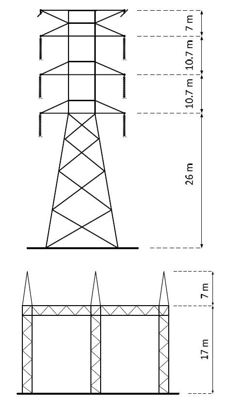
The selection of the electric power cable as well as other parameters is made on the basis of technical specification of the company Tele-Fonika Kable S.A: A2XS (FL) 2Y2Y-GC-FR 1x2000RMS/210 64/110 (123) kV IEC 60840
Table 1.
Current in the main conductor
Air temperature
Ground temperature
Distance from the ground surface
[A]
[oC]
[oC]
[m]
940
+35
+8
+8
.
Figure 1 presents the numerical model of the analyzed system, and in Figure 2 − the temperature profile for the typical boundary conditions of the system Table 1 where assumed thermal conductivity is λ=1[W/mK].
Fig.1. FEM model of the analyzed system
There are substantial visible differences in temperature in the core of the cable for the earth thermal conductivity λz∈0,2÷0,8 [W/mK] Fig.4, additionally assumed boundary conditions for 40o C.
Fig.2. The temperature distribution in the ground and the maximum temperature of the core (for boundary conditions of Chart 1)
Fig.3. The temperature distribution in the ground, and analyzed the system (for boundary conditions of Chart 1)
Fig.4. Temperature changes in the core of the cable at different depths (from 1 to 8 m) for different values of thermal conductivity (from 0,22 to 1,2)
Figure 5. presents the temperature profile in the core, screen and surface of the cable at different depths.
The temperature profile stabilizes starting at 10m and temperature differences between its individual layers are constant at different depths.
Fig.5. The analysis of temperature profile in the core of the cable for different depths (1-40m)
Conclusions
As a result of the conducted computer simulation and the analysis of the temperature profile in the system depending on its distance from the surface of the earth and its thermal conductivity which is affected by different temperatures on the surface it is necessary to state the following:
➣ the thermal conductivity of earth has substantial influence on the temperature of the core of the cable – up to the value of 0,8 [W/mK] ➣ the temperature in the core of the cable is determined starting at depth of 10 m ➣ the differences in temperatures between the core of the cable, its screen and the surface are constant for the defined boundary conditions and average between 6o C and 2o C, as well as can be defined after exceeding the depth of 10m ➣ the influence of the outer temperatures on the temperature profile inside the cable stabilizes below 10 m from the surface
REFERENCES
[1] Kącki E. Równania różniczkowe cząstkowe w elektrotechnice WNT Warszawa 1968 [2] L. Kacejko, Cz. Karwat, H. Wójcik: Laboratorium techniki wysokich napiec, WPL [3] S. Szpor: Technika wysokich napiec, WNT Warszawa [4] Z . Flisowski: Technika wysokich napiec, WNT Warszawa [5] Z . Gacek: Wysokonapieciowa technika izolacyjna, WPS Gliwice [6] Khajavi M., Zenger W ., Desing and commissioning of a 230 kV cross linked [7] polyethylene insulated cable system, JICABLE 2003,paper A .1.1, Paris 2003 [8] Toya A ., Kobashi K., Okuyoma Y., Sakuma S., Higher stress desingned XLPE insulated cable in Japan, General Session CIGRE 2004, paper B1-111 [9] Suzuki A ., Nakamura S., Tanaka H., Installation of the world’s first 500 kV XLPE cable with intermediate joints, Furukawa Review, No 19, 2000 [10] Rakowska A ., Najnowsze osiągnięcia w dziedzinie kabli wysokiego napięcia. Stosowanie żył miedzianych w kablach na napięcie 110 kV i wyŜsze, XII Konferencja Naukowo – Techniczna Elektroenergetyczne linie kablowe i napowietrzne Kabel 2005 [11] Granadino R., Plans J., Schell F., Undergrounding the first 400 kV transmission Line in Spain using 2500 mm2 XLPE cables, JICABLE 2003, paper A .1.2, Paris 2003 [12] Jones S.L., Bucea G., Jinno A ., 330 kV cable system for the MetroGrid project In Sydney Australia, CIGRE General Session 2004, paper B1 – 302
Author: Janusz Tykocki, The State College of Computer Science and Business Administration in Lomza, Akademicka 14, 18-400 Lomza, Poland. E-mail: jtykocki@pwsip.edu.pl
Source & Publisher Item Identifier: PRZEGLĄD ELEKTROTECHNICZNY (Electrical Review), ISSN 0033-2097, R. 87 NR 12b/2011
Published by Electrotek Concepts, Inc., PQSoft Case Study: Commercial Facility Harmonic Evaluation, Document ID: PQS1005, Date: March 15, 2010.
Abstract: Utility power system harmonic problems can often be solved using a comprehensive approach including site surveys, harmonic measurements, and computer simulations.
This case study presents the results for a commercial facility harmonic evaluation. The simulations were completed using the PSCAD program. The analysis evaluates the effects of transformer connections to determine the harmonic current distortion levels on both the primary and secondary sides of the customer transformers. The simulation results show the third harmonic neutral current and a K-Factor transformer derating analysis.
INTRODUCTION
A commercial facility harmonic evaluation was completed for the system shown in Figure 1. The case study was completed using the PSCAD program. The accuracy of the simulation model was verified using three-phase and single-line-to-ground fault currents and other steady-state quantities.
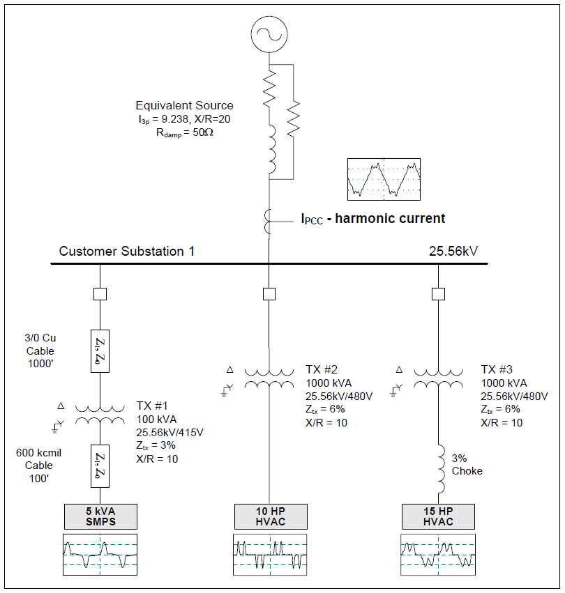
The circuit model for the case involved a 25.56kV customer substation with two 1,000 kVA step-down transformers supplying HVAC loads and one 100 kVA transformer supplying switch-mode power supply (SMPS) loads.
Figure 1 – Illustration of Oneline Diagram for Commercial Facility Harmonic Evaluation
Switch-mode power supplies use dc/dc conversion techniques for maintaining constant dc voltage output. In the absence of a large ac-side inductance, input current to the power supply becomes positive and negative current pulses, characterized by high crest factors (peak to rms ratio) and high harmonic content. A high third harmonic current content is especially typical of switch-mode power supplies. Since third harmonic current components do not cancel each other in the neutral of a three-phase system, increasing application of switch-mode power supplies has created a concern for overloading of neutral conductors, especially in older buildings where an undersized neutral may have been utilized.
SIMULATION RESULTS
The case study evaluates the effects of transformer connections to determine the harmonic current distortion levels on both the primary and secondary sides of the customer transformers. Figure 2 shows the simulated power supply current and the resulting current on the transformer primary due to the delta/wye connection that traps the zero sequence harmonics in the primary delta winding.
The secondary power supply current has a fundamental frequency value of 6.76 amps, an rms value of 8.10 amps, and a THD value of 66.12%. The highest component was the 3rd harmonic with a value of 62.30%. The resulting primary transformer current has fundamental frequency value of 0.15 amps, an rms value of 0.16 amps, and a THD value of 14.89%. The highest components were the 5th harmonic with a value of 12.93% and the 7th harmonic with a value of 6.39%.
Figure 3 shows the transformer derating and K-Factor calculations. The assumed eddy current loss factor (PEC-R) for the dry type 100 kVA transformer was 8%. A K-Rating of four would be sufficient for this application.
Figure 4 shows the transformer neutral current when supplying the power supply loads. The phase A power supply current is also shown for reference. The triplen harmonics add in the neutral to create a waveform that that consists of mostly 3rd harmonic (180 Hz) frequency. The rms value of the neutral current was 12.72 amps, with the highest components being the 3rd at 12.63 amps, the 9th at 1.41 amps, and the 15th at 0.25 amps. One mistake commonly made with this type of waveform is to use a THD value in percent. This is because the fundamental frequency component of the neutral current in a balanced system approaches zero amps, which leads to a THD value that approaches infinity.
Figure 2 – Simulated Power Supply and Transformer Primary Currents
Figure 3 – Power Supply Transformer Derating Calculation
Figure 4 – Simulated Transformer Neutral
Figure 5 shows the simulated HVAC #1 current and the resulting current on the transformer primary. The secondary current has a fundamental frequency value of 13.10 amps, an rms value of 24.12 amps, and a THD value of 154.58%.
Figure 5 – Simulated Drive #1 and Transformer Primary Currents
Figure 6 shows the simulated HVAC #2 current and the resulting current on the transformer primary. The secondary current has a fundamental frequency value of 16.18 amps, an rms value of 18.57 amps, and a THD value of 56.44%.
Figure 6 – Simulated Drive #2 and Transformer Primary Currents
Figure 7 shows the simulated point of common coupling (PCC) current at the utility/customer interface. The current has a fundamental frequency value of 3.73 amps, an rms value of 3.74 amps, and a THD value of 8.18%. The highest components were the 5th harmonic with a value of 3.99%, the 7th harmonic with a value of 4.30%, the 11th with a value of 4.05%, and the 13th with a value of 2.89%. The values of the triplen harmonics (e.g., 3rd, 9th, 15th, etc.) were negligible due to the fact that all of the transformers supplying the nonlinear customer loads have delta connected primary windings and also that all of the customer loads were balanced.
Figure 7 – Simulated Point of Common Coupling Current
SUMMARY
This case study summarizes the results for a commercial facility harmonic evaluation. The case study evaluates the effects of transformers connections to determine the harmonic current distortion levels on both the primary and secondary sides of the customer transformers. The simulation results show the third harmonic neutral current and a K-Factor transformer derating analysis. The simulation results also highlight the effect of harmonic current cancellation that may occur in a facility which results in lower distortion at the point of common coupling.
REFERENCES
Power System Harmonics, IEEE Tutorial Course, 84 EH0221-2-PWR, 1984.
IEEE Recommended Practice for Monitoring Electric Power Quality,” IEEE Std. 1159-1995, IEEE, October 1995, ISBN: 1-55937-549-3.
IEEE Recommended Practices and Requirements for Harmonic Control in Electrical Power Systems, IEEE Std. 519-1992, IEEE, ISBN: 1-5593-7239-7.
RELATED STANDARDS IEEE Std. 519-1992 IEEE Std. 1159-1995
GLOSSARY AND ACRONYMS ASD: Adjustable-Speed Drive CF: Crest Factor DFT: Discreet Fourier Transform DPF: Displacement Power Factor PCC: Point of Common Coupling PF: Power Factor PWM: Pulse Width Modulation TDD: Total Demand Distortion THD: Total Harmonic Distortion TPF: True Power Factor
Published by Mark KLETSEL1, Nariman KABDUALIYEV2, Bauyrzhan MASHRAPOV2, Alexander NEFTISSOV2, National Research Tomsk Polytechnic University (1), Pavlodar State University (2)
doi:10.12915/pe.2014.01.21
Abstract. A phase comparison scheme of protection of busbar on the reed switches fixed connections near conductors extending from these busbars which does not require current transformers has been studied. The article provides an analysis of its sensitivity and behavior in different modes
Streszczenie. Porównano metody zabezpieczeń przewodów szynowych przełączników kontaktronowych. Uwzględniono przypadki gdy nie jest stosowany przekładnik prądowy. (Zabezpieczenia szynowych przełączników kontaktronowych)
Keywords: busbar, protection, reed switch, phase comparison, current transformer. Słowa kluczowe: szyna, zabezpieczenie, kontaktron.
Introduction
It is known that damages on busbars have serious consequences. Most dangerous of them are short circuits through an arc (both – uniphase and interphase), especially in cells of switchgears (distributing devices) [1, 2, 3]. There is rather large number of methods and the devices revealing uniphase short circuits on earth, for example [4]. There is much less sensing protections that reveal two-phase short-circuits. It is possible to include to them logical [5] and differential [6] protections of busbars. And all of them receive information from current transformers which have a number of well-known shortcomings [7, 8]. In this regard works in the direction of creation of the protection which are not using current transformers, for example [9,10] are already conducted. As it was noted at the last international CIGRE conferences [8, 11] because of an incompleteness of these works they are actual and now. Offered protection of busbar (Fig. 1) is one of results of continuation of works in the direction of creation of protection on magnetooperated contacts – reed switches which have explicitly explained in [8, 12, 13, 14] advantages over other magnetooperated elements.
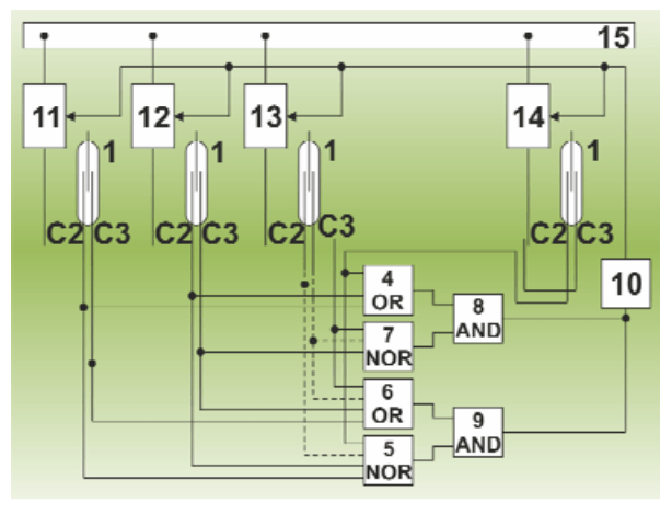
Model of protection
In the flowchart (Fig. 1) Protection 1 – polarized with a reed contact (С) 2 and 3 are installed in a magnetic field of different phase conductors of similar connections are connected to the busbars 15 so that one of the current halfwaves, e.g. positive, closed С 2, and the other- to 3. Contacts 2 are connected to the inputs of the OR gate 4 and the NOR 5 and С 3 – to the inputs of OR element 6 and a NOR 7, the outputs of elements 4 and 7 are connected to AND gate 8, the outputs of elements 5 and 6 – and to 9, the outputs of the elements 8 and 9 – to the executive body of the 10 applicable at the circuit breakers 11-14 connections.
Operation principle
The apparatus operates as follows. In the load mode, and an external short circuit current polarity, at least one of the connections in any half-cycle does not match the polarity of the remaining currents. When the reed switch is closed to 2 this connection, 3 reed switches are closed to other bays, and when the second current half-closed C 3, on the other accessions are closed to 2. As a result, any time the reed switch is closed and the reed switch C 2 C 3 closed. Therefore, the outputs of the elements 5 and 7 and there is no signal as a result, no signals at the outputs of the elements 8 and 9. Executive body of the 10 does not work. If a short circuit on the tire 15 in a single half-closed only to 2 on all connections (connections of all the currents are in phase), the other – to 3. With the closure of C 2 and the lack of contact closure outputs for 3 items 4 and 7, there are signals that the body 10 is triggered. When the closure to the insulation 3 and C 2 signals appear at the outputs of the elements 5 and 6. Thus, whatever the current half cycle is not a short circuit, the device comes into effect at that moment. Due to the high speed, it may qualify for use as a busbar 500 and 750 kV.
Provision of reed switches operation polarity
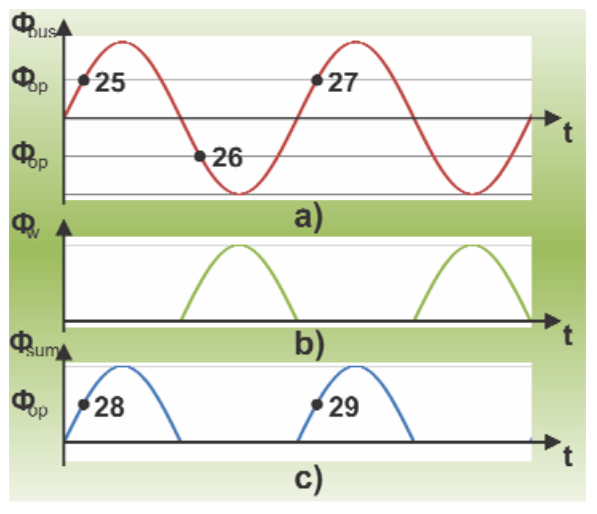
Polarized reed switches in the circuit can be used only if N ≤ 3, where N is the multiplicity of the short-circuit current with respect to the tire, where the reed switch is activated. The fact is that when N > 3 demagnetized permanent magnet, which is an integral part of the reed switch. Therefore, if N > 3 should go on complication – one reed used instead of two with normally open contacts 16 and 17 with two windings 18 and 19, but instead of С 2 and 3 – to 20 and reed switches 16 and 21, 17 respectively. In this case, the winding 18 is a source of EMF, and 19 to compensate for the actions of one of the half-wave voltage. Output windings 19 are connected to the inputs of amplifier 22, amplifier outputs – to the input phase comparison circuit 23 outputs circuits 23 – via a diode 24 to the control winding 19. The polarity switching reed contact [12] is provided as follows. The magnetic flux Φbus (Fig. 3a), created by = alternating current Ibus in bus, for example, phase A connection 12, is the EMF E=-dΦbus/dt output winding 18, which is fed to an amplifier 22. Image EMF must be such that the magnetic flux Φw created by current Iw in the winding 19 is equal to the amplitude of Φbus. EMF in the circuit 23 is shifted in phase by 90 degrees so that the winding 19 Iw coincided in phase with the current Ibus. The polarity of the winding connections 19 to the output circuit 23 should be such that the magnetic flux Φw was directed opposite tensions flow Φbus. Diode 24 passes only one of the half-wave voltage in the winding 19. Consequently, the current in the winding Iw appears only in this half-wave. Figure 3 shows the flow of the Φbus and the Φw and the amount of magnetic flux Φsum acting on the reed switch, and Φop – magnetic flux at which the reed switch is activated. If you do not use the coil 19, the reed switch 16 operates in both half-wave alternating current at Φbus = Φop corresponding to points 25, 26, 27 (Fig. 3a). When a current Iw in the winding 19 on the reed switch 16 acts Φsum = Φbus + Φw that allows it to fire only one half-wave of the alternating current in phase A connection 12.
Sensitivity
For comparison, the currents in the corresponding phases of the connections should be located close to their international conductors so as to eliminate the influence of the currents of neighboring phases. To ensure the safety, distance should not be less than the permissible value. For the closing of the reed switch without replacement within 10 years, it is necessary to their operation occurred at currents exceeding the maximum load currents [11]. Besides Reed them selves have limited sensitivity of m.m.f. response. All this in significantly extent limits the sensitivity of the busbar protection for reed switches [11], and to improve it requires the use of reed switches with a large resource of operation P ≥ 1010 and a small m.m.f.
Fig.1. Protection scheme
Fig.2. Way of provision of operation polarity
Fig.3. Magnetic flows: a) and b) created by current in phase (bus) and winding 19; c) summary.
Application of protection
For application of this protection devices are necessary that allow to mount (fix) the reed such way, that it makes possible to change distance from reed to phase current conductors (busbars) and angle of inclination towards to them (such constructions are known, for example [15, 16]). At the same time to avoid the influence of adjacent (nearby) phases it’s necessary to choose parameters of reeds’ arrangement in accordance with the calculation in [14].
Conclusion
The proposed busbar protection does not require current transformers and has high speed, but its sensitivity is dependent on the lifetime of the reed switch and m.m.f.
REFERENCES
[1] Stanisław Maziarz, Jerzy Szynol, Examining the conditions of eliminating hazard due to arc faults inside switchgears and transformer stations, Przeglad Elektrotechniczny, 2001, nr. 3, pg.62-65. [2] Roman Partyka, Daniel Kowalak, The effects of fault-arc in medium voltage gas isolated switchboards installed on ships, Przeglad Elektrotechniczny, 2013, nr. 8, 290-293. [3] Małgorzata Bielówka, Experimental measurements of the fault arc parameters, Przeglad Elektrotechniczny, 2008, nr. 4, 98-101. [4] Lubomir Marciniak, Application of signal wavelet decomposition for identification of arc earth faults, Przeglad Elektrotechniczny, 2011, nr. 2, 101-104. [5] G. Bolgartsev, Mark Kletsel, Konstantin Nikitin, V. Matokhin, The device for the centralized current protection of a network, USSR Author Certificate #1644287, 1991, nr. 15. [6] Kang Y.C., Lim U.J., Kang S.H., Crossley P.A., A busbar differential protection relay suitable for use with measurement type current transformers, Ieee Transactions on Power Delivery, 2005, nr. 20/2, 1291-1298. [7] Xuesong Zhou, Zhihao Zhou, Youjie Ma, Dongfang Wu, Analysis of Excitation Current in DC-Biased Transformer by Wavelet Transform, Przeglad Elektrotechniczny, 2012, nr 5b, 108-112. [8] Mark Kletsel, Bases of creation of relay protection on reed switches, Collection of reports of the International scientific and technical conference (Ekaterinburg), 2013,posters sector 10. [9] Marcin Habrych , Bogdan Miedziński , Hassan Nouri , Witold Dzierżanowski, Performance of ground fault protection using Hall sensor under real conditions of operation, Przeglad Elektrotechniczny, 2010, nr. 7, 181-183. [10] Krzysztof Ludwinek, Measurement of momentary currents by Hall linear sensor, Przeglad Elektrotechniczny, 2009, nr. 10, 182-187. [11] L. Kozhovich, M. Bishop, The modern relay protection with current sensors on the basis of the coil Rogovsky. The modern directions of development of systems of relay protection and automatic equipment of power supply systems, Collection of reports of the International scientific and technical conference (Moscow), 2009, 49-59. [12] Mark Kletsel, The principles of construction and model of differential protection on reed switches, Russian Electrical Engineering, 1991, nr. 10, 47-50. [13] Mark Kletsel, J. Alishev, A. Manukovsky, Properties of reed switches applied in relay protection, Electrical Technology Russia, 1993, nr. 9, 18-21. [14] Mark Kletsel, Pavel Maishev, Features of construction on reed switches of differential and phase protection of transformers, Russian Electrical Engineering, 2007, nr. 12, 2-7. [15] Innovative patent Republic of Kazakhstan No. 19636 Measuring body for relay protection of three-phase symmetric current distributors of 6-35 KV / Mark Kletsel, Assemgul Zhantlesova, Bibigul Zhantlesova : the applicant and the patent holder – the Pavlodar state university named after S.Toraighyrov (KZ). — No. 2006/0882.1; declared 31.07.2006; published 16.06.2008, Bulletin No. 6. — 6 pages [16] Innovative patent Republic of Kazakhstan No. 20265 Measuring body for relay protection of three-phase symmetric current distributors of 6-10 KV / Mark Kletsel, Assemgul Zhantlesova, Bibigul Zhantlesova, Nurlan Erzhanov : the applicant and the patent holder – the Pavlodar state university named after S.Toraighyrov (KZ). — No. 2006/1351.1; declared 01.12.2006; published 17.11.2008, Bulletin No. 11. — 5 pages
Authors: prof. doctor of technical sciences mr. Mark Kletsel, National Research Tomsk Polytechnic University, Tomsk, Russian Federation, E-mail: Mark2002@mail.ru; mr. Nariman Kabdualiyev, Pavlodar State University, Electroenergetics Faculty, Pavlodar, Lomov str., 64, Republic of Kazakhstan, E-mail: kaznar@mail.ru; mr. Bauyrzhan Mashrapov, Pavlodar State University, Electroenergetics Faculty, Pavlodar, Lomov str., 64, Republic of Kazakhstan, E-mail: bokamashrapov@mail.ru; mr. Alexander Neftissov, Pavlodar State University, Electroenergetics Faculty, Pavlodar, Lomov str., 64, Republic of Kazakhstan, E-mail: shurikneftisov@mail.ru.
Source & Publisher Item Identifier: PRZEGLĄD ELEKTROTECHNICZNY, ISSN 0033-2097, R. 90 NR 1/2014
Published by Electrotek Concepts, Inc., PQSoft Case Study: Arc Furnace Harmonic Evaluation, Document ID: PQS1004, Date: March 15, 2010.
Abstract: Utility power system harmonic problems can often be solved using a comprehensive approach including site surveys, harmonic measurements, and computer simulations.
This case study presents the results for an arc furnace harmonic evaluation. The case study was completed using the SuperHarm program. The simulation results show harmonic resonances that increase voltage distortion levels when the utility substation capacitor bank was in service.
INTRODUCTION
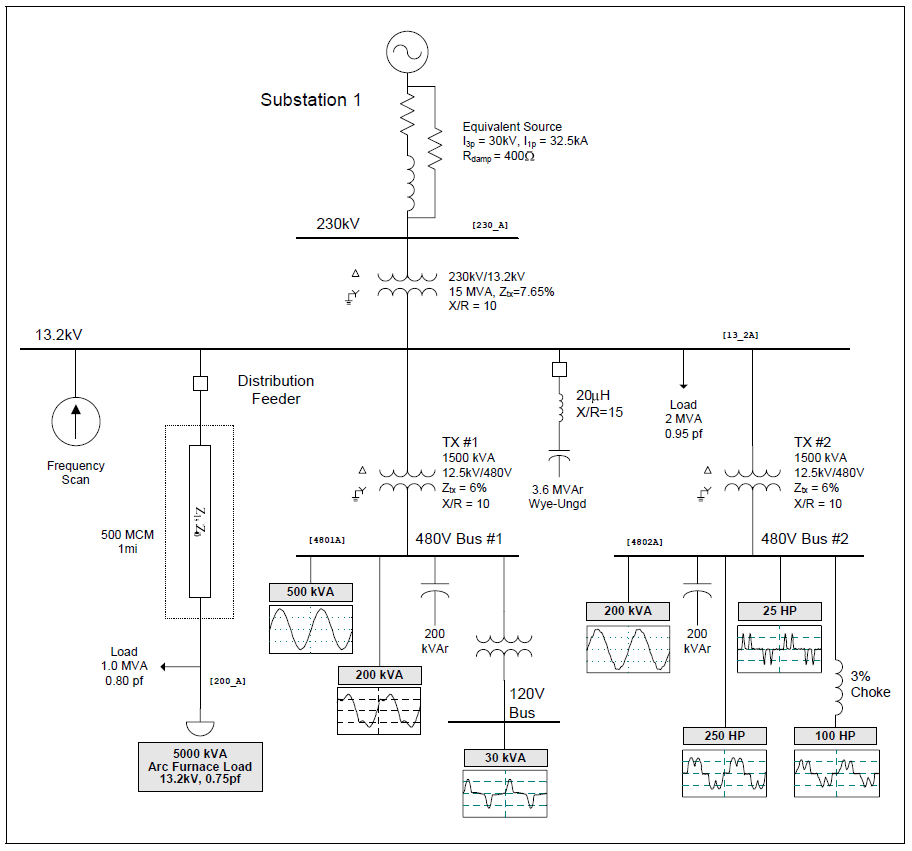
An arc furnace harmonic evaluation study was completed for the system shown in Figure 1. The case study was completed using the SuperHarm program. The accuracy of the simulation model was verified using three-phase and single-line-to-ground fault currents and other steady-state quantities.
The circuit modeled for the case involved a 230kV/13.2kV utility substation supplying two 1,500 kVA customer step-down transformers and one 5,000 kVA arc furnace load. Each customer has a switchable 200 kVAr, 480-volt capacitor bank and a variety of nonlinear loads.
Figure 1 – Illustration of Oneline Diagram for Arc Furnace Harmonic Evaluation
SIMULATION RESULTS
Relevant utility system and customer data for the case included:
Substation capacitor bank rating: 3.6 MVAr Substation load: 2.0 MVA, 0.95 pf Feeder load: 1.0 MVA, 0.80 pf Customer capacitor bank ratings: 200 kVAr Miscellaneous linear load: 700 kVA Fluorescent lighting (ITHD = 21.7%): 200 kVA DC drive (ITHD = 35.3%): 250 hp PWM ASD (no choke – ITHD = 130.8%): 25 hp PWM ASD (with 3% choke – ITHD = 45.1%): 100 hp Switch mode power supplies (ITHD = 77.2%): 30 kVA
Figure 2 shows the simulated current waveform (single phase shown) for the 5,000 kVA, 13.2kV arc furnace operating at a 75% power factor. The current has a fundamental frequency value of 209 amps, an rms value of 224 amps, and a THD value of 35.2%. The simulated arc furnace characteristic represents a measured 18-cycle snapshot of one operating point for the arc furnace. The waveform shown in Figure 2 was created using an inverse DFT with 256 points per cycle.
Figure 2 – Arc Furnace Current Waveform
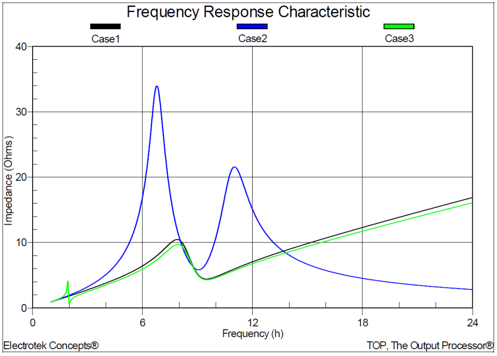
Figure 3 shows the results for the three frequency scan simulations. Case #1 was the base case with no utility capacitor banks included in the model. Case #2 was the case with the 3.6 MVAr on the 13.2kV substation bus in service. Case #3 was the case with the 3.6 MVAr capacitor bank reconfigured as 2nd harmonic filter. The parallel resonances for Case #2 were about 407 Hz (6.8th) and 660 Hz (11th).
The tuning of the harmonic filter near the 2nd harmonic was required due to the lower frequency components included in the arc furnace current. Arc furnace applications may require less common types of harmonic filters, such as series passive, low-pass broadband, and c-type. A c-type filter may be used for complex loads such as cycloconverters and electric arc furnaces.
Figure 3 – Simulated Customer Frequency Response Characteristics
Table 1 summarizes the results for the three distortion simulations. The table includes the simulated voltage distortion (THD) at the five buses for the three different operating conditions. A number of locations exceed the voltage limitation of 5% THD. Adding the 13.2kV, 3.6 MVAr substation capacitor bank in Case 2 caused the two customer 480-volt buses to exceed 5% THD. Reconfiguring the capacitor bank as a 2nd harmonic filter in Case 3 reduced the voltage distortion on the customer buses to below 5% THD.
Table 1 – Summary of the Simulated Voltage Distortion Results
Case Number
13.2kV Bus
13.2kV Feeder
480V Bus #1
480V Bus #2
120V Bus #1
1
2.288%
5.902%
2.478%
4.828%
3.808%
2
3.439%
6.478%
5.780%
7.151%
5.286%
3
2.191%
5.790%
2.353%
4.713%
3.766%
.
Figure 4 shows the simulated 3.6 MVAr capacitor bank current for the Case 2 operating condition. The current has a fundamental frequency value of 130 amps, an rms value of 132 amps, and a THD value of 18.5%.
Figure 4 – Simulated Capacitor Bank Current
SUMMARY
This case study summarizes the results for an arc furnace harmonic evaluation. The simulation results show harmonic resonances that increase voltage distortion levels when the utility substation capacitor bank was in service. The initial solution might seem to be to install a 5th harmonic filter; however, filters should be tuned below the lowest significant harmonic being generated. In this case, that was the 2nd harmonic.
REFERENCES
Power System Harmonics, IEEE Tutorial Course, 84 EH0221-2-PWR, 1984.
IEEE Recommended Practice for Monitoring Electric Power Quality,” IEEE Std. 1159-1995, IEEE, October 1995, ISBN: 1-55937-549-3.
IEEE Recommended Practices and Requirements for Harmonic Control in Electrical Power Systems, IEEE Std. 519-1992, IEEE, ISBN: 1-5593-7239-7.
RELATED STANDARDS IEEE Std. 519-1992 IEEE Std. 1159-1995
GLOSSARY AND ACRONYMS ASD: Adjustable-Speed Drive CF: Crest Factor DFT: Discreet Fourier Transform DPF: Displacement Power Factor PCC: Point of Common Coupling PF: Power Factor PWM: Pulse Width Modulation TDD: Total Demand Distortion THD: Total Harmonic Distortion TPF: True Power Factor
Published by Muhammad MANSOOR, Norman MARIUN, Napsiah ISMAIL, Noor Izzri ABDULWAHAB, Faculty of Engineering, University Putra Malaysia (UPM)
Abstract. This paper proposes a concept of knowledge engineering based innovative approach for seeking solutions related to electrical engineering systems. The knowledge base approach is discussed for its effectiveness at preliminary stages of solution hunting and solution design, which may reduce the iterations of design process and save time/cost. While referring research literature, this paper builds a hypothesis for novel and efficient usage of knowledge engineering tools for Electrical Engineers. The research seeks development of a methodological tool, which will be generic for aimed sub-sector (e.g. power distribution) of electrical systems. Based on structured innovation approach, this tool will provide conceptual guidance and direction to find solutions in sector specific electrical system problems. This structured approach and electrical engineering focus of the tool will facilitate electrical engineers for reaching practical and effective solutions with less expertise and time.
Streszczenie. W artykule zaproponowano zastosowanie metod inżynierii wiedzy do rozwiązywania problemów związanych z systemami elektrycznymi. Pozwala to na ograniczenie liczby iteracji przy projektowaniu i skraca czas projektu. (Zastosowanie metod inżynierii wiedzy w projektowaniu systemów elektrycznych)
If we look around in our surroundings, we see a lot of different engineering systems added in our life over the passage of time. All engineering systems e.g telephone, Televisions, Generators, Vehicles, Aero planes etc, are examples of technological creativity and innovation adding value to human life. These inventions are output of a continuous process starting from a feel of need and originating as a solution idea in human mind. Engineering is the process of turning those ideas into reality by defining the concepts and implementing those into physical systems/products. This creative act of turning ideas into technological concepts and ultimately into a complete product is called engineering design. Most of the existing inventions/systems are output of creative human efforts which didn’t exist before or are improvements in some previously existing systems. For reasons, the engineers are known as “problem solvers”, who address some need/problem of a current scenario and are supposed to come up with some practical solution. Coming to engineering design problems, there may be more than one possible solution for some problem and engineers are needed to bring up the best feasible solution considering all the requirements of problem [1]. Competitive market, always growing complexity of High-Tech equipment, need of higher quality power for sensitive equipments and integration of diversified technological components in one electrical system is making electrical engineer’s solution hunting tougher as ever.
Engineering design
Engineering Design in its nature is an iterative process [2], as the engineers work towards building a solution concept and implementing the concept as physical system. The most suitable and desired design solution is the one that most completely meets the requirements and can be delivered at right time, within feasible cost and with the available resources.
Engineers need to turn backward and forward again and again to refine and develop the real system for best possible solution according to requirements. During this backward forward process, design activities can be seen as activities based on successive decision making which enables the design process to converge towards a solution. This iterative process consumes time as well as costs for reaching the ultimate desired physical output. A good solution requires a good methodology or process of meeting the design aims, which makes the engineers consider all the requirements and helps in dealing all the obstacles in reaching the best output in “least time” with “least costs”, while using “available resources”.
There are multiple design methodologies defined by different researchers over the time which vary a little bit in approach of addressing the design problem or steps to converge the activities towards a solution. Out of different methodologies, this research concept shall consider following “kind of generic 5-steps” of engineering design process [1].
1- Define the Problem, 2- Gather Information, 3- Generate Multiple Ideas, 4- Analyze and select a solution, 5- Test and Implement.
Following above generic engineering design process steps, it is proposed to bring a novel approach of incorporating the emerging knowledge engineering methodology TRIZ (The Theory of Inventive Problem solving) with electrical solutions design process. It’ll facilitate Electrical Engineers as problem solvers using strong TRIZ knowledge base.
Complexity of Electrical Engineering Systems and TRIZ
As discussed above, at one hand, Engineers as problem solvers are supposed to bring best possible solutions meeting all requirements with least cost, time and resources. On the other hand, with the growing age of technology, engineering systems are becoming more and more complex and difficult to handle. The complexity of Electrical engineering systems and integration of different technologies (e.g. Electrical devices, Electronic devices, ICT equipment, Automation equipment etc) as part of one engineering system makes it very challenging for engineers to understand the root cause of problems and come up with better solutions. Much higher expertise and knowledge of multiple fields are required to seek a comprehensive efficient solution, which ultimately need bigger project teams with higher expertise at behalf of engineers (problem solvers). To reduce this complexity and facilitate Electrical Engineers, TRIZ do offer an efficient set of tools and methods. It doesn’t only reduce complexity of problem solving rather it offers systematic guidance for bringing the innovative solutions for the problems.
As discussed in [3], in process of finding solution for an engineering problem, the project team is supposed to tackle a problem which is usually characterized by many requirements and objectives, some of which are conflicting. Often the team has to deal with problems with no known solution. Such a problem is called an inventive problem and may also contain contradictory requirements. To find a successful solution for an inventive problem, Knowledge and creativity are two essential conditions. In real practice often there is a lack of both of these key characteristics. For dealing with complex integrated systems, the project teams are usually consisting of interdisciplinary expertise. But still it is virtually impossible to integrate universal knowledge of all specialized areas into one team. Also research studies have shown that creativity diminishes steadily throughout the work phase of life and people hesitate to be creative, because they fear that they lack the essential skills. The usual human approach towards solving problems is by analogical thinking. That is, we try to relate the problem we are facing to some standard class of problems (analogs) we are familiar with, and for which a known solution exists. If we can draw the right analogy, we can find the right solution. Our knowledge of such analogous problems, however, is the result of our educational, professional, and life experiences. Ideally, all potential directions for solutions should be equally regarded. But as an output of field specific knowledge, expertise and experiences, only solutions derived from one’s personal knowledge and familiarity are considered while the consideration of alternative technologies (the innovative thinking) to develop new concepts is ignored. This results in what is called psychological inertia, which lacks randomness and leads only into those areas of personal experience. For electrical engineering solutions, it would be a decisive advantage if the team had an extensive knowledge base and was capable of generating innovative concepts purposefully and systematically, rather than more or less at random [3]-[4].
TRIZ brings the concept of step wise systematic innovation while addressing conflicting requirements, technical contradictions, requirement of multidisciplinary expertise, hesitancy towards being creative, psychological inertia problems of project team through its systematic innovation methods and wide range of strong tools. TRIZ expands the knowledge horizon of the developer by using a scientific-engineering knowledge base and supports the user systematically throughout the process of creative problem solving. The method ensures an effective and efficient search for innovative solutions, focusing on the so called Ideal Final Result. It limits the search field considerably, but fosters creativity within that search field. [4].
Research literature provides some good examples where different Knowledge Engineering tools of artificial intelligence as well as TRIZ have been used effectively for problem solving of electrical and related engineering domains e.g. novel electrical devices development, innovative approach towards product and process designs, Electrical energy saving, quality planning and energy conservation/saving practices [7-14].
Proposed research development
During the solution design, while pursuing the Engineering Design process, considering the defined problem, its’ core reasons and surrounding elements/important factors to keep in view, a conceptual design is sought for the solution. This conceptual design can be considered as some kind of qualitative (nonquantitative) design at initial design stage. Usually more than one solution come up for some specific problem which is to be analyzed against the requirements and best suitable solution is chosen for implementation. The detailed design with specific parameters’ quantitative evaluation and implementation follows the non-quantitative/conceptual design stage. The process progresses through these stages in an iterative manner. At each of these stages the product design exists in distinct level of available information which is called a “design state” [5]. The complete design process is a kind of process which is based on successive decision making, this successive decision making ultimately leads towards a solution.
This research proposes that at initial design process activities (which can be grouped as conceptual design phase), incorporating TRIZ tools will help electrical engineers breaking the mindset, while bringing more practical and innovative ideas. This integration of TRIZ at conceptual design phase will ultimately make engineers reach a good conceptual design systematically. This will be leading towards an innovative and practical solution by helping them make the “right decisions at every successive stage/activity” hence saving time, cost and unnecessary iterations. Taking help with TRIZ methodology at initial design stages is like “sharpening the axe before cutting the tree”. TRIZ sharpens your axe the best and it takes very little effort to cut the tree (find the suitable innovative and practical solution).
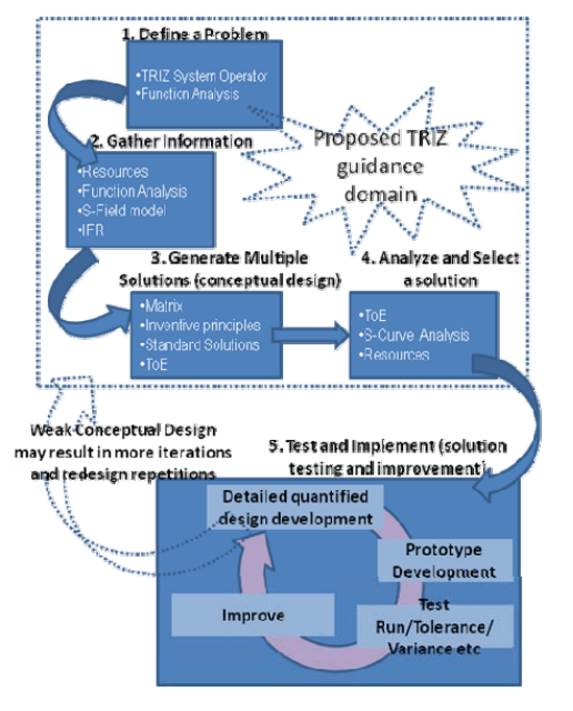
Fig. 1. Proposed TRIZ analysis for Electrical Engineering Problems
The proposed development further aims at simplifying Electrical Engineering solutions’ design process and leading the engineers towards “potential future” innovative solutions. To cater deficiencies and limitations in today’s Electrical systems and to guide Electrical engineers towards future solutions, this research proposes that analysis of current electrical problems (e.g. power distribution sector) and available solutions by TRIZ knowledge base toolset will result in sector specific guidelines for future solutions (As depicted in Fig. 1). TRIZ concepts of “Trends of engineering system evolution” and “S-curve analysis” will result in conceptual framework for looking forward to right future innovation. It will help in breaking limitations and contradictions existing in current available solutions related to Electrical engineering problems. The proposed analysis of sector specific Electrical Engineering problems along with their current available solutions by tools and knowledge base of TRIZ will simplify problem identification, solution exploration and conceptual design for Electrical engineers. Problem definition tools of TRIZ (system operator, Function Analysis, Ideal Final result (IFR) etc) have potential for reaching the right problem and root cause for that problem which should be addressed. IFR helps seeing whole of the picture and directs towards bringing an optimum performance solution. Problem solving tools of TRIZ (Contradiction Matrix, Inventive principles, standard solutions, S-field analysis etc), lead towards breaking mindsets and exploring the solution space beyond field specific expertise of solution seekers.
S-curve, Trends of evolution can assess the current status and foresee the conceptual direction for potential future solutions related to current Electrical engineering problems [6]. This all helps in building the right conceptual design before entering into quantitative design phase where parameters quantifications, testing and implementation can cost a lot more time if the conceptual stage doesn’t bring a strong output. Improvements needing iteration/repetition for design activities can consume unnecessary time and funds, if the initial solution sought is having deficiencies. Furthermore, this comprehensive analysis of sector specific problems in particular Electrical engineering domain, may work as “generic guideline” for conceptual stage design process for that sector specific problems. This will result in ease for Electrical engineers working in that specific domain of electrical engineering, hunting the needed solutions with generic guidance extracted and modified from TRIZ knowledge base. After successful outcome of one sector, the research may further be extended to different Electrical Engineering domains, producing more comprehensive and generic guidelines for electrical engineers in future. TRIZ guidance domain for Electrical Engineers may be depicted as in Fig. 2. The figure shows different TRIZ tools which can help at referred generic design stages. The proposed research output will be a set of guidelines which will take electrical engineers through initial design stages for reaching an innovative and effective conceptual design.
Fig. 2. TRIZ guidance domain for Electrical Engineering solution design
Conclusions
The emerging Knowledge Engineering tool TRIZ has potential to produce good qualitative improvements to electrical engineering solution design process. It can reduce complexity of solution seeking process for electrical engineers, guiding them to innovative and effective solutions in a structured systematic way. By reducing complexity, breaking psychological inertia for innovative thinking and expanding solution search space of engineers across their own field of expertise, it guides engineers to make right decision and reach an effective conceptual design before entering into quantitative phase. Development of sector specific guidelines by analysis of electrical engineering ‘sector specific’ problems using TRIZ toolset, will lead towards more focused, more simplified, faster results oriented, innovative and systematic guidelines pertinent to a specific electrical engineering segment. After successful outcome of one sector, the research may further be extended to different electrical engineering domains, producing more comprehensive and generic guidelines for electrical engineers in future.
REFERENCES
[1] S. Khandani, “Engineering Design Process, ”IISME/Solectron, 2005. [2] Dekker D.L., Engineering design processes, problem solving and creativity, Frontiers in Education Conference, Proceedings 1 (1995), 3a5.16-3a5.19. [3] Mansoor M., Towards a model/framework for optimizing automated engineering systems in developing countries, Proceedings of TRIZCON 2008. [4] Pfeifer T., Tillmann M., Innovative process chain optimization – utilizing the tools of TRIZ and TOC for manufacturing, ETRIA World Conference- TRIZ Future 2003. [5] Eisenbart B., Gericke K., Blessing L. T. M., A framework for comparing design modelling approaches across disciplines, Proceedings of the 18th International Conference on Engineering Design, 2 (2011), 344–355. [6] Mann D., Hands on systematic innovation, (2002), CREAX Press:Belgium. [7] Zhang F. Y., Xu Y. S., He Q. P., Research on product systematic innovative design based on TRIZ, Materials Science Forum, (2006), 532-533:761-764. [8] Lakshminarayanan K., Holistic value framework – creating right value streams using TRIZ and other concepts, The TRIZ Journal, Online Article Achives 1 (2007). [9] Zhang X., Chen D., A conceptual design approach generated by integrating AD and TRIZ into the conceptual design phase of SAPB, Advanced Materials Research, (2010), 118-120:977-981. [10] Zhang F. Y., Zhang H. C., Zheng H., Zhang Q. Q., Energysaving product innovative design process based on TRIZ/AD, Proceedings of IEEE 17th International Conference on Industrial Engineering and Engineering Management, (2010), 325-328. [11] Wakaiki S., Adachi K., Kotaki H., Practical application of TRIZ to novel electrical devices development, Japan TRIZ Society 4Th TRIZ Symposium, (2008) Laforet Biwako, Japan. [12] Randall M., Rob V.D.T., 40 Principles of TRIZ and the Electric Power Grid, The TRIZ Journal, Online Article Archives, 2 (2010). [13] Sharifi-Tehrani O., Novel hardware-efficient design of LMSbased adaptive FIR filter utilizing finite state machine and block-RAM, Przeglad Elektrotechniczny, 87 (2011), no.7, 240-244. [14] Drabarek J., Artificial intelligence methods in data protection techniques, Przeglad Elektrotechniczny, 87 (2011), n. 10, 133-135
Authors: Mr Muhammad Mansoor, Department of Electrical & Electronics Engineering, Faculty of Engineering, University Putra Malaysia, 43400 Serdang, Selangor, Malaysia,Email: mansoor.upm@gmail.com; Prof Dr. Norman Mariun, Department of Electrical & Electronics Engineering, Faculty of Engineering, University Putra Malaysia, 43400 Serdang, Selangor, Malaysia,Email: norman@eng.upm.edu.my (Corresponding Author); Prof Dr Napsiah Ismail, Department of Mechanical & Manufacturing Engineering, Faculty of Engineering, University Putra Malaysia, 43400 Serdang, Selangor, Malaysia, Email: napsiah@eng.upm.edu.my; Dr Noor Izzri AbdulWahab, Department of Electrical & Electronics Engineering, Faculty of Engineering, University Putra Malaysia, 43400 Serdang, Selangor, Malaysia, Email: izzri@eng.upm.edu.my
Source & Publisher Item Identifier: PRZEGLĄD ELEKTROTECHNICZNY (Electrical Review), ISSN 0033-2097, R. 88 NR 11a/2012
Published by Electrotek Concepts, Inc., PQSoft Case Study: Substation Transformer Switching and Dynamic Overvoltages, Document ID: PQS1204, Date: January 26, 2012.
Abstract: This case study presents the results for a wind plant substation transformer energizing and dynamic overvoltage evaluation. Transformer inrush currents contain harmonic components that may create dynamic overvoltages if a substation transformer is energized with a collector circuit or capacitor bank on the secondary bus. Mitigation alternatives for this problem include energizing a capacitor bank separately from the transformer and energizing the transformer/capacitor bank combination with enough secondary loads to sufficiently damp the transient overvoltages.
INTRODUCTION
A wind plant substation transformer energizing and dynamic overvoltage transient analysis case study was completed for the system shown in Figure 1. The case study investigated transformer energizing transients and the potential for excessive dynamic overvoltages due to resonances created by collector circuit cables or substation capacitor banks. The simulations were completed using the PSCAD® transient program. A transient model was created to simulate a wind plant collector circuit and the resulting transient voltages and currents during transformer switching events.
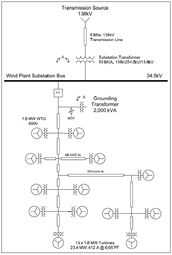
Figure 1 – Illustration of Oneline Diagram for Transformer Switching Analysis
SIMULATION ANALYSIS
The simulation model included a 138kV wind plant substation and a 6-mile transmission line supplying a 50 MVA, 138/34.5/13.8 kV substation transformer. The substation included a 138kV circuit breaker on the transformer high-side bus and an 8 MVAr, 34.5kV capacitor bank on the collector circuit bus. There was one 34.5kV collector circuit included in the model.
The model was designed so transformer energizing transients and the potential for excessive dynamic overvoltages due to resonances created by collector circuit cables or substation capacitor banks could be determined. The accuracy of the simulation model at 60 Hz was determined using simulated fault current magnitudes and other steady-state quantities, such as cable line charging (MVAr) and feeder load flow values (MW & MVAr). The representation of the system short-circuit equivalent at the 138kV source substation, under assumed normal system conditions, included:
Three-phase (I3φ) fault current: 17,500 A @ -85.0° (4183 MVA) Single-line-to-ground (IφG) fault current: 20,000 A @ -85.0° (4780 MVA)
These values were converted to ohms for the PSCAD representation, which included a three-phase voltage source with positive and zero sequence impedances. The 6.0 mile, 138kV transmission line was modeled using the following data:
Length: 6.0 mi Positive sequence impedance (Z1): 0.11660 +j0.68140 Ω/mi Zero sequence impedance (Z0): 0.40245 +j2.72030 Ω/mi Positive sequence line charging (XC1): 0.168142 MΩ-mi Zero sequence line charging (XC0): 0.296228 MΩ-mi
The coupled π-section model was used to model the transmission line. That assured accurate representation of both the series impedances, as well as the line charging characteristics of the transmission line. The coupled π-section is primarily used to represent short overhead transmission lines or underground cables.
The substation transformer was modeled using the classical three-phase, three-winding transformer model. The nameplate impedance data for the substation transformer included:
%Z1 @ 50 MVA, 138/34.5/13.8kV
% R
% X
Primary – Secondary (H-X)
0.320
8.50
Primary – Tertiary (H-Y)
0.400
10.00
Secondary – Tertiary (X-Y)
0.020
4.00
.
%Z0 @ 50 MVA, 138/34.5/13.8kV
% R
% X
Primary – Secondary (H-X)
0.320
8.00
Primary – Tertiary (H-Y)
0.400
9.00
Secondary – Tertiary (X-Y)
0.020
3.50
.
The 34.5kV collector circuit cable sections were included in the transient model using the following impedance data:
Conductor: 500 kcmil AL Length: 2,000 feet Positive sequence impedance (Z1): 0.0499 +j0.0553 Ω/1000’ Zero sequence impedance (Z0): 0.1508 +j0.0599 Ω/1000’ Line charging (B/2): 11.5 μmhos/1000’
Conductor: 4/0 AWG AL Length: 1,000 feet Positive sequence impedance (Z1): 0.1087 +j0.0653 Ω/1000’ Zero sequence impedance (Z0): 0.2567 +j0.0688 Ω/1000’ Line charging (B/2): 8.7 μmhos/1000’
It was assumed that positive and zero sequence line charging values were the same. The coupled π-section model was used to model each cable section. That assured accurate representation of both the series impedances, as well as the line charging of the collector system cables.
The peak magnitude and duration of the transformer inrush current is dependent on a number of factors, including, the point on the voltage waveform when the switch contact is closed, the impedance of the circuit supplying the transformer, the value of the residual flux in the core, and the nonlinear magnetic saturation characteristic of the transformer core. Typical transient inrush current magnitudes for energizing unloaded transformers are 5-10 times the rated transformer current. However, these values may be somewhat lower when energizing a transformer from a relatively weak
The substation transformer was modeled using the three-phase, three-winding classical transformer model. The nonlinear portion (saturation) of the transformer characteristic was included by specifying three parameters of the core saturation characteristic. The air core reactance of the transformer was 0.2 per-unit, the knee voltage was 1.2 per-unit, and the magnetizing current was 0.1%. The calculated full load current (high-side) for the transformer is 210 amps.
The three circuit breaker closing times were selected to be three successive phase voltage zero values so the worst-case inrush currents, without residual flux, would be simulated. The equivalent source voltage for the transformer inrush case was adjusted so that the pre-switching voltage magnitude at the transformer high-side would be 1.05 per-unit (105%).
Case 1 involved energizing the substation transformer with no collector circuits or capacitor banks inservice (unloaded). This was the initial basecase to determine the transformer energizing transient inrush current magnitude. Figure 2 shows the simulated three-phase transformer primary inrush current for Case 1, while Figure 3 highlights the Phase A current. The peak transient current magnitude was 818.9 amps.
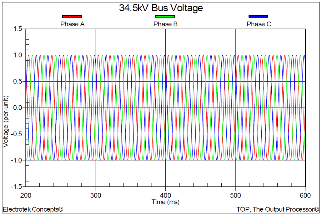
Figure 4 shows the three-phase 34.5kV transformer secondary voltages for Case 1. The peak voltage is 1.05 per-unit. There were no dynamic overvoltages during the energizing event without any capacitance connected to the transformer secondary winding.
Figure 2 – Simulated Three-Phase Transformer Energizing Current for Case 1
Figure 3 – Simulated Transformer Energizing Current (Phase A) for Case 1
Figure 4 – Simulated Substation Transformer Secondary Voltage for Case 1
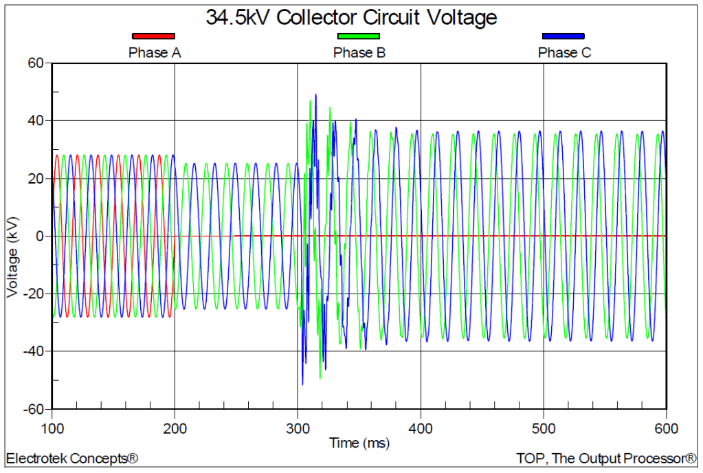
Case 2 involved energizing the substation transformer with the 34.5kV collector circuit in service. The peak transient current magnitude was 822.8 amps. Figure 5 shows the resulting three-phase 34.5kV transformer secondary voltages for Case 2.
The peak transient voltage on the transformer secondary bus increased to 1.33 per-unit with the collector circuit in-service for Case 2. This value is below the assumed protective levels of most typical surge arresters (e.g., MSSPL ~ 1.90 per-unit), so it is anticipated that the arresters would not operate for this condition.
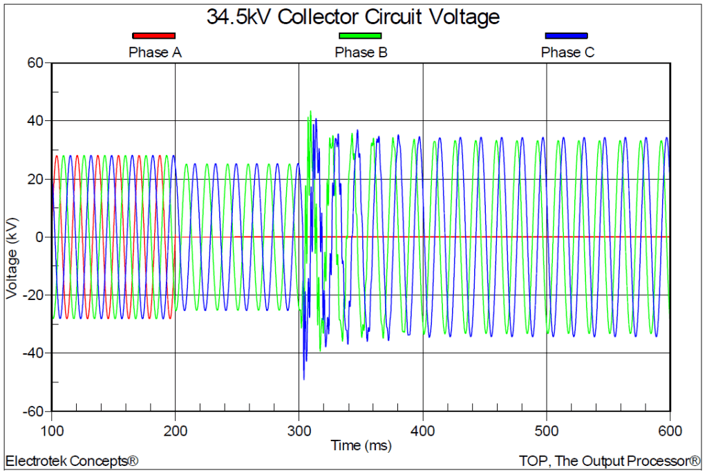
Case 3 involved energizing the substation transformer with both the 34.5kV collector circuit and an 8 MVAr, 34.5kV capacitor bank in-service. The peak transient current magnitude was 968.6 amps. Figure 6 shows the resulting three-phase 34.5kV transformer secondary voltages for Case 3.
The maximum transient voltage on the transformer secondary bus increased to 1.45 per – unit with the substation capacitor bank and collector circuit in-service for Case 3. This value is below the assumed protective levels of most typical surge arresters (e.g., MSSPL ~ 1.90 per-unit), so it is anticipated that the arresters would not operate for this condition.
Figure 5 – Simulated Substation Transformer Secondary Voltage for Case 2
Figure 6 – Simulated Substation Transformer Secondary Voltage for Case 3
SUMMARY
This case study presented a wind plant substation transformer energizing and dynamic overvoltage evaluation. Transformer inrush currents contain harmonic components that may create dynamic overvoltages if a substation transformer is energized with a collector circuit or capacitor bank on the secondary bus.
Mitigation alternatives for this problem include energizing a capacitor bank separately from the transformer and energizing the transformer/capacitor bank combination with enough secondary loads to sufficiently damp the transient overvoltages. The concern for dynamic overvoltages is typically limited to cases of energizing large substation transformers with large power factor correction capacitor banks.
The simulation results highlight a concern for dynamic overvoltages when the substation transformer is energized from the primary side with the 34.5kV collector circuit or 8 MVAr capacitor bank in-service. The peak transient voltage on the transformer secondary 34.5kV bus was 1.33 per-unit with the collector circuit in-service and 1.45 per-unit with both the collector circuit and capacitor bank in-service. The transient voltages were below typical surge arrester protective levels (e.g., MSSPL ~ 1.9 per-unit), so it is anticipated that MOV surge arresters would not operate during substation transformer energizing with the simulated circuit conditions.
REFERENCES
IEEE Recommended Practice for Grounding of Industrial and Commercial Power Systems, IEEE Std. 142 (IEEE Green Book), IEEE, November 2007, ISBN: 0738156392.
IEEE Recommended Practice for Monitoring Electric Power Quality,” IEEE Std. 1159-1995, IEEE, October 1995, ISBN: 1-55937-549-3.
IEEE Recommended Practices and Requirements for Harmonic Control in Electrical Power Systems, IEEE Std. 519-1992, IEEE, ISBN: 1-5593-7239-7.
RELATED STANDARDS IEEE Std. 1159
GLOSSARY AND ACRONYMS DFT: Discreet Fourier Transform PCC: Point of Common Coupling TDD: Total Demand Distortion TOV: Temporary Overvoltage
All repetitive waveforms can be composed of combinations of many sinusoidal waves. Any waveform can be analyzed to determine the component quantities. In this article, learn how to use Fourier Analysis to determine the amplitudes of harmonic components and their phase relationship to the fundamental component in various periodic non-sinusoidal waveforms.
A harmonic is a frequency that is an integer (whole number) multiple (second, third, fourth, etc.) of the fundamental frequency. The fundamental frequency on power distribution lines is 60 Hz and changes from positive to negative 60 cycles per second. For instance, the second harmonic on a 60 Hz power distribution line is 120 (60 × 2) Hz. The second harmonic waveform completes two cycles during one cycle of the fundamental waveform over the same period of time.
Figure 1. A harmonic is a frequency that is an integer (whole number) multiple (second, third, fourth, fifth, etc.) of the fundamental frequency. Image used courtesy of Amna Ahmad
Fourier analysis (developed by mathematician Jean Fourier) is a mathematical operation that analyzes the waveforms to determine their harmonic content. Each harmonic’s amplitude, as well as its phase relationship to the fundamental, can be determined. Also, the level of any DC component can be computed.
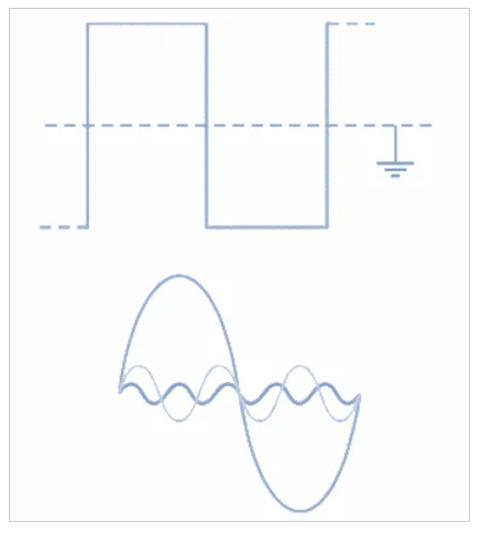
Square Wave
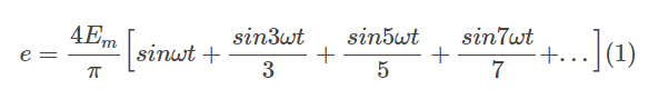
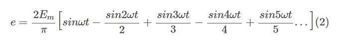
A pure square wave, symmetrical above and below ground level [Figure 2], can be shown by Fourier analysis to be represented by the following equation:
.
where
e is an instantaneous value at time t 4Em/π is the peak value of a waveform sinωt is a Fundamental component sin3ωt/3 is a Third harmonic sin5ωt/5is a Fifth harmonic sin7ωt/7 is a Seventh harmonic
As shown by the equation, a symmetrical square wave can be made up of fundamental component and odd harmonics but has no even harmonics and no DC component.
Figure 2. Harmonic analysis of a symmetrical square wave shows that it contains fundamental and odd harmonics. Image used courtesy of Amna Ahmad
NOTE: Fourier analysis can be applied to all repetitive waveforms to determine their harmonic content.
Sawtooth Wave
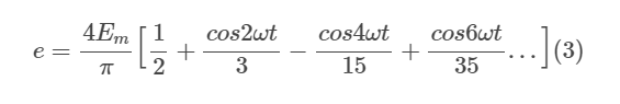
The Fourier equation for the sawtooth waveform in Figure 3 is
.
In this case, all the harmonics are present, and again, there is no DC component. In general, a waveform has no DC component when it is symmetrical above and below ground level.
Figure 3. Harmonic analysis of a symmetrical sawtooth wave reveals that it is composed of a fundamental and all harmonics. Image used courtesy of Amna Ahmad
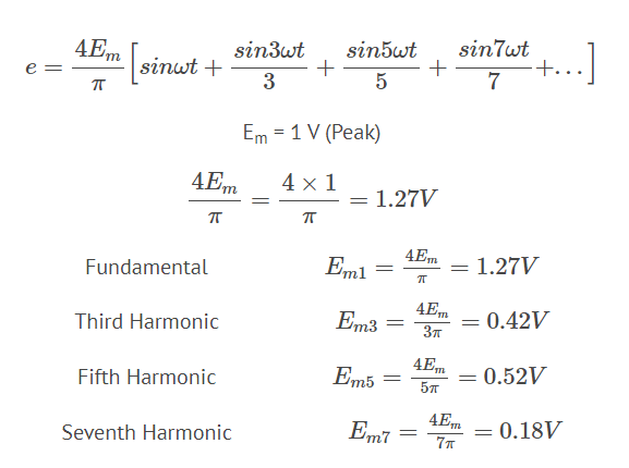
Rectified Wave
The full-wave rectified sine wave in Figure 4 can be represented by
.
Figure 4. A full-wave rectified sine wave comprises a DC component and even harmonics that decrease in amplitude with increasing harmonic number. Image used courtesy of Amna Ahmad
Equation 3 shows that the waveform has a DC component 4Em/2π and even harmonics, 2ωt, 4ωt, 6ωt, and so on ( Figure 4). It would appear there is no fundamental frequency component. However, in this case, the fundamental frequency is taken as the input frequency (f) of the waveform prior to rectification. It could be argued that the fundamental frequency of the rectified waveform is actually 2f. For example, a 60 Hz sine wave, when full-wave rectified, produces a succession of sinusoidal half-cycles with a frequency of 120 Hz.
Amplitudes of Harmonics
Examination of the equations for the square, sawtooth, and rectified sine wave shows that in all cases, the amplitudes of the harmonic components decrease as the harmonic frequency increases. Thus, the higher-order harmonics appear to have decreasing importance. This is certainly true in terms of the contribution of these components to the rms value of the waveform and to the power dissipated in a load. However, for good reproduction of the waveform, many of the higher-order harmonics must be present. For example, in the case of a square wave, all components up to the eleventh harmonic (or higher) may be required. For a pulse waveform, harmonics up to the one hundredth may have to be present to create a good output wave shape.
Square Wave Example
A square wave with a 2 V peak-to-peak amplitude is symmetrical above and below ground level. Calculate the amplitudes of each component up to the seventh harmonic.
Solution.
From equation (1),
.
Note that the harmonic voltage components calculated are all peak values. Each must be multiplied by 0.707 to determine the rms values.
Rectified Sine Wave Example
A full-wave rectified sine wave has a peak amplitude of 30 V and a (pre-rectified) frequency of 60 Hz. Calculate the DC component and the rms values of the harmonic components up to the sixth harmonic. Also, determine the harmonic frequencies.
Solution.
From equation (3),
.
Conclusion
With harmonic analysis, periodic non-sinusoidal waveforms can be shown to consist of combinations of pure sine waves, sometimes with a DC component. One main component, a large-amplitude sine wave having the same frequency as the periodic wave being analyzed, is the fundamental. The other components are sine waves with frequencies that are exact multiples of the fundamental frequency. These waves, denoted as harmonics, are numbered according to the ratio of their frequency to that of the fundamental.
Author: Amna Ahmad is an Electrical Engineer with a major emphasis in Control and Energy Systems.
Published by Marcin SZEWCZYK, Tomasz KUCZEK, Mariusz STOSUR, Wojciech PIASECKI, Marek FLORKOWSKI, Marek FULCZYK, ABB Corporate Research Center in Krakow, Poland
Abstract. In the present paper simulations of the propagation of lightning overvoltages in a typical HV GIS substation are presented. The influence of HV LC filter on maximum overvoltages peak values was analyzed. Additionally, an improvement to the surge protection by using a HV filtering element introduced at the connecting point between the GIS substation and the transmission line has been proposed.
Streszczenie. W artykule przedstawiono symulacje wyładowań atmosferycznych i propagacji fali przepięciowej w typowej stacji GIS wysokiego napięcia. Zaprezentowano możliwość zapewnienia dodatkowej ochrony przeciwprzepięciowej poprzez ograniczenie maksymalnej wartości przepięć za pomocą wysokonapięciowego filtra w miejscu połączenia przesyłowej linii napowietrznej ze stacją GIS. (Wpływ filtra LC wysokiego napięcia na ograniczenie przepięć piorunowych w stacjach gazowych typu GIS)
Studies of power systems involving lightning surge phenomena are performed to design transmission lines and substations as well as for the insulation coordination of power system equipment. Lightning overvoltages are generated by a current stroke to a tower structure, which results in complex surge phenomena propagating throughout the transmission lines and substations. An overvoltage is a voltage wave which is superimposed on the rated voltage of the network. It is characterized by: the magnitude (in kV), the rise time (in μs) and the rate of rise called steepness (in kV/μs). Overvoltages which can disturb electrical installations and loads can have lightning or switching origin.
GIS substations are protected against switching and lightning overvoltages by means of surge arresters. The protective levels of the arresters are selected so that the overvoltages appearing at the protected elements are lower than the corresponding insulation coordination levels.
In insulation coordination practice an assumption is made that in all cases an air insulated surge arrester (AIS) is obligatory, and is installed at the gantry of the substation. A GIS surge arrester, installed at the transformer terminal, is also required.
Due to the fact that lightning phenomenon is by nature high frequency, special modeling approaches have to be applied. This paper describes modeling principles of frequency dependent elements using the ATP/EMTP software package. A typical system consisting of a high voltage transmission line and a 400 kV GIS substation has been modeled. Lightning phenomena including both direct stroke and back-flash stroke have been simulated for HV LC filter working conditions in order to evaluate key factors influencing the maximum overvoltage peak values.
Models of studied system
An incoming 23 km overhead transmission line was represented by a frequency dependent JMarti model. It was implemented in the ATP/EMTP software with the Line/Cable Constants subroutine [1].
Two parallel lines with conductors per bundle were introduced, as presented in Figure 1. During the lightning strike an overvoltage wave is generated, which propagates and deflects at any point of discontinuity. For this reason it is important to model 5 separate spans of overhead line (400 m each) counting from the portal tower (gantry). A propagating surge wave can be also deflected from the tower base, thus the tower footing resistance (TFR) was implemented as a constant value of resistance equal to 20 Ω. The tower structure (Fig.1) was represented by means of a lossless distributed parameter line, which consists of a surge impedance equal to 172 Ω, a wave propagation speed of 290 m/μs and an associated height. The portal tower (Fig. 1) surge impedance value was equal to 70 Ω [1,4-5].
Fig.1. Tower and gantry structure layouts for 400 kV system
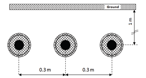
The HV cable that interconnects the GIS substation with the overhead transmission line has a length equal to 5 km, whereas the cable between GIS substation and power transformer is 0.2 km long. Both cables were modeled as frequency dependent elements with Line/Cable Constants subroutine [1-2]. A flat formation with 0.3 m spacing between each cable and 1 m vertical depth position were used. Its arrangement and basic parameters are presented in Figure 2 and Table 1.
Table 1. HV cable data [5]
Parameter
Value
conductor cross section
2500 mm2
XLPE insulation thickness
25.8 mm
XLPE relative permittivity
2.5
overall diameter
146 mm
.
Fig.2. HV cable arrangement
Due to the high frequency nature of the lightning phenomenon, various pieces of substation equipment were modeled as appropriate phase-to-ground capacitances Cp-g [pF] and surge impedances Z [Ω] with associated length L [m] and wave propagation speed v [m/μs]. Values used in the analyses are given in Table 2.
Table 2. Substation apparatus data [5]
Apparatus
Parameters
GIS busbars
Z = 60 Ω, v = 290 m/μs
310 MVA transformer 400 kV terminals
2000 pF
circuit breaker
50 pF
GIS spacer
15 pF
.
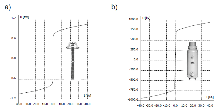
Fig.3. Voltage-current characteristics at 8/20 μs current impulse for surge arresters; a) air insulated (AIS), b) gas insulated (GIS)
For the overvoltage mitigation purposes both air and gas insulated surge arresters are installed in a substation. In the model they are represented by nonlinear U-I characteristics at 8/20 μs current surge, as presented in Figure 3. Lead lengths and phase-to-ground capacitances have been added, 1 μH/m and 25 pF respectively.
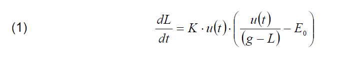
The insulators are represented by the Leader Progression Model. This model considers an equivalent leader, which propagates along the insulator. Back-flash occurs when the leader length reaches length of the insulator gap (assumed to 4.5 m) in specific time equal to that of real leaders. The leader velocity and its propagation are described by a formula (1) given by [4]:
.
where: K – constant [m2/([kV]2· s)], E0 – average gradient voltage [kV/m], u(t) – voltage across the gap [kV], g – gap length [m], L – leader length [m].
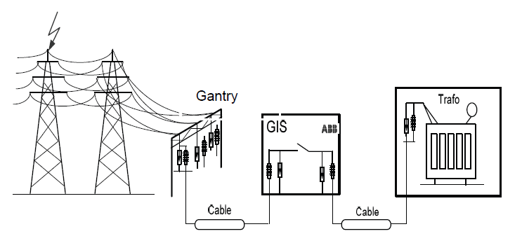
Studies
The studied 400 kV network consists of two parallel incoming transmission lines, a GIS substation and HV cables that interconnect the GIS substation with overhead lines (5 km) and the GIS substation with power transformer (0.2 km). An air insulated surge arrester is installed at the portal tower, whereas gas insulated surge arresters are connected at the GIS substation and HV terminals of 310 MVA transformer (Fig.4). A new solution has also been introduced. It was proposed to install a passive overvoltage mitigating device at the portal tower (Fig.4), comprising a high voltage LC low-pass filter [6].
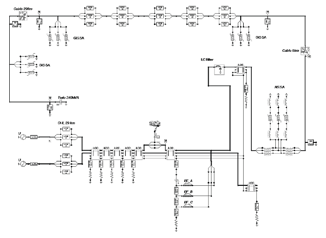
Fig.4. General network overview
Lightning strokes occurring at the overhead transmission lines incoming at the 400 kV GIS substation have been simulated by means of CIGRE wave shape [2]. Two different scenarios and lightning current magnitudes were used:
– direct stroke to the phase wire with 30 kA current, – stroke to shield wire causing back-flash across the insulator chain to the phase wire with 200 kA current.
For each case maximum overvoltage peak values have been calculated and compared to the Basic Insulation Level (BIL) of 1425 kV [3-4].
ATP/EMTP simulation results
The objective of these studies was to analyze the influence of HV LC filter on overvoltages in a typical power network consisting of an overhead line (OHL), cables and GIS substation as well as to select such parameters, which are the most appropriate for mitigation of Fast Transients in a GIS substation.
Table 3. Scope of work
Overvoltage mitigation device
Run 1 – Fig.6
Run 2 – Fig. 7
AIS surge arrester
connected
connected
LC filter
connected
not connected
GIS surge arrester at substation entrance
not connected
connected
GIS surge arrester at substation exit
not connected
connected
GIS surge arrester at Transformer HV terminals
not connected
connected
.
The parameter optimization analysis was performed for a typical 400 kV GIS substation in which the HV filter has been applied in order to mitigate Fast Transients caused by lightning strokes. The HV LC filter has been located between overhead line (OHL) and HV cables that interconnect a GIS substation (Fig.4). For each of the above cases, voltages in three points were observed: at the transformer terminal (TRAFO), the GIS entrance (GIS IN) and the GIS exit (GIS OUT). A detailed scope of work was presented in Table 3.
The ATP/EMTP model of the 400 kV power network and GIS substation involved in the simulations is shown in Figure 5.
Fig.5. Typical 400 kV GIS substation model implemented to ATP/EMTP software (corresponding to Figure 4)
The Fast Transients analyses were performed in order to check the effectiveness of the HV LC filter at suppressing the overvoltages that occurred during lightning strokes [7]. The following scenarios with respect to the scope of work from Table 3 have been considered:
• BF Tower 2 – back-flash at tower 2, • BT Tower 3 – back-flash at tower 3, • DS 50 m – direct stroke 50 m from tower 1, • DS 300 m – direct stroke 300 m from tower 1.
The maximum overvoltage peak values for the simulated cases are summarized in Figure 6 (run 1). For comparison, results for normal cases in system (without HV LC filter) are given in Figure 7 (run 2).
Fig.6. Fast Transient overvoltages maximum values at the three locations (TRAFO, GIS IN, GIS OUT), for worst cases (Tab. 3) – without GIS surge arresters in system, LC filter connected
Fig.7. Fast Transient overvoltages maximum values at the three locations (TRAFO, GIS IN, GIS OUT), for normal cases – AIS and GIS surge arresters in system, without LC filter
Overvoltages have been calculated at the three points of consideration and for different surge arresters combinations as presented in Table 3 with reference to diagram illustrated in Figure 5.
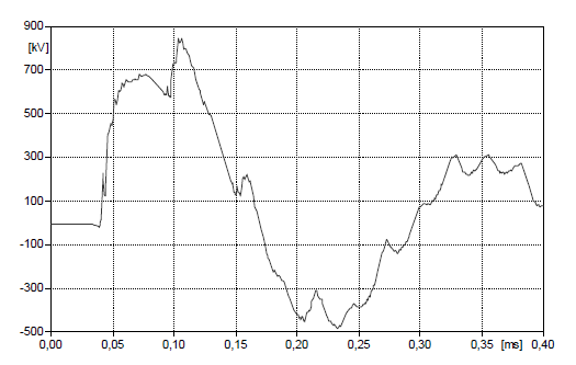
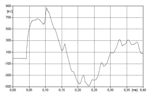
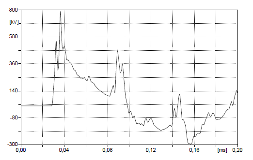
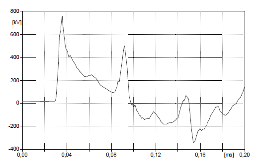
Calculated ATP/EMTP simulation waveforms are presented in Figures 8 to 13.
Fig.8. Overvoltage waveform at transformer HV terminals, back-flash at tower 2
Fig.9. Overvoltage waveform at GIS entrance, back-flash at tower 2
Fig.10. Overvoltage waveform at GIS exit, back-flash at tower 2
Fig.11. Overvoltage waveform at transformer HV terminals GIS exit, direct stroke, 50 m from tower 1
Fig.12. Overvoltage waveform at GIS entrance, direct stroke, 50 m from tower 1
Fig.13. Overvoltage waveform at GIS exit, direct stroke, 50 m from tower 1
It has been determined that in the system studied, it is potentially possible to omit the installation of GIS surge arresters in the power system. When only the GIS surge arresters within the GIS substation are omitted (i.e. when the only surge arresters are: the AIS SA at the gantry and the GIS SA at the transformer terminal), the overvoltages are below the insulation coordination level (80% of BIL) (Fig.6). Hence, the GIS surge arresters within the GIS substation of interest are optional.
For further reduction of the overvoltages and for improving the insulation coordination margin, a HV LC filter can be applied. The reduction is substantial for direct strokes, for which the insulation coordination level is exceeded when only the AIS surge arrester at the gantry is applied. In this case the insulation coordination margin can be achieved by adding the GIS surge arrester at the transformer terminal. The proposed additional solution is a passive element consisting of a line trap main coil (L) and a coupling capacitor (C). It has been proven that the proposed filter provides sufficient insulation coordination margins.
Conclusions
The Insulation Coordination study for a typical system consisting of 400 kV GIS substation interconnected by a HV cables has been performed using the ATP/EMTP software. Back-flash and direct stroke scenarios for lightning overvoltage analyses were studied. The overvoltages have been calculated at essential points of the substation: at the transformer HV terminal, substation entrance and substation exit.
An alternative solution to the use of an additional GIS surge arrester has been proposed. The passive element consisting of a line trap main coil and a coupling capacitor installed at the portal tower have been introduced. It should be noted that when the HV LC filter was installed the lightning overvoltages were kept below the BIL, especially in the worst cases where all GIS surge arresters in the power system were not installed. Hence it is suggested to use the solution proposed as an additional transient mitigation device.
REFERENCES
[1] Dommel H.W., Electromagnetic Transients Program, Reference Manual (EMTP) Theory Book, BPA, Portland, Oregon, (1986) [2] CIGRE WG33.0, Guide to procedure for estimating the lightning performance of transmission lines, CIGRE brochure 63, Oct. (1991) [3] IEC 60071-1:2006, Insulation co-ordination – Part 1: Definitions, principles and rules [4] Andrew R. Hileman, Insulation Coordination for Power Systems, CRC Press Taylor and Francis Group, New York, (1999) [5] IEEE Fast Front Transients Task Force, Modeling Guidelines for Fast Front Transients, IEEE Transactions on Power Delivery, Vol. 11, pp. 493-506, Jan. 1996 [6] S tosur M. et al., Impact of high voltage GIS substation configuration on lightning overvoltages, NIWE-11 Conference, Sept. (2011) (a copy in print for Electrical Review) [7] IEC 60099-4:2009, Surge arresters – Part 4: Metal-oxide surge arresters without gaps for a.c. systems
Authors: Marcin Szewczyk, Ph.D. Eng. E-mail: marcin.szewczyk@pl.abb.com; Tomasz Kuczek, M.Sc. Eng. E-mail: tomasz.kuczek@pl.abb.com; Mariusz Stosur, Ph.D. Eng. E-mail: mariusz.stosur@pl.abb.com; Wojciech Piasecki, Ph.D. Eng. E-mail: wojciech.piasecki@pl.abb.com; Marek Florkowski, D.Sc. Eng. E-mail: marek.florkowski@pl.abb.com; Marek Fulczyk, Ph.D. Eng. E-mail: marek.fulczyk@pl.abb.com; ABB Corporate Research Center, Starowiślna 13A Str., 31-038 Kraków, Poland;
Source & Publisher Item Identifier: PRZEGLĄD ELEKTROTECHNICZNY (Electrical Review), ISSN 0033-2097, R. 88 NR 5a/2012
Published by Norberto ANGULO1, Antonio PULIDO1, Felipe DÍAZ1, Fabián DÉNIZ1, Expedito SÁNCHEZ1, Rafael SÁNCHEZ2, Universidad de Las Palmas de Gran Canaria (1), Mancomunidad del Sureste de Gran Canaria (2)
Abstract. The main aim of this paper is to determine the photovoltaic capacity of Gran Canaria Island, part of the Canary Islands, an archipelago with high levels of solar irradiation. The method: an individual research focused on each municipality of the island, calculating the energy to be produced by each of them, separately. From the analysis, it can be concluded that the best option for PV in the island is the building integrated systems, especially the roof integrated ones.
Streszczenie. Celem pracy jest określenie możliwości fotowoltaicznych wispy Gran Canaria w archipelago wysp Kanaryjskich o bardzo dużym nasłonecznieniu. W konkluzji stwierdzono że najlepszym rozwiązaniem jest budowa zintegrowanego systemu dachowego. (Dachowy zintegrowany system fotowoltaiczny na wyspach Kanaryjskich)
Keywords: Solar energy; Distributed Generation; Roof Integrated PV Systems. Słowa kluczowe: energia słoneczna, system c=dachowy.
Introduction
The enviable geographical location of the Canary Islands is characterized by high levels of solar irradiation; making the archipelago a suitable region to host photovoltaic systems. However, the current implantation of this systems on land is unviable due to the limitations of the territory (7529 km2), the high rates of population (2.100.000 inhabitants, January 2010), and the abundance of protected areas (46% of the surface). Therefore, the future of photovoltaic energy within the Canary Islands in general; and within the island of Gran Canaria in particular; comes along with the construction of photovoltaic systems on top of the buildings, connected to the main network. Each building would host low power systems, what, in addition, would allow the decentralization of the electricity generation; and the consequent improvement of the current power system, increasing its output.
PV in Spain in general and in the Canary Islands in particular begins to be implemented in a serious way since 2004 as a result of the emergence of a regulatory framework providing a bonus for the generation through renewable energy sources (RD 436/2004).
One year later, the Spanish Government launched a detailed plan for introducing renewable energy generation systems. This plan, known as “Plan de Energías Renovables” (PER), set the expected numbers of the photovoltaic energy in Spain: 400 MW installed for 2010, and therefore, 363 MW to be installed within a period of 5 years (2005-2010). This plan specified as well the scheduled installed power in Canarias for 2010, 17,24MW; what meant the installation of 16,04MW within 5 years, a 93% of the total power.
The Canary Islands Government, in order to adapt its energy policy to the dictates of the Spanish Government, in 2006 created the “Plan Energético de Canarias” also known as PECAN. It tried to make possible, the installation of power in the Archipelago through renewable energy to reduce the dependence on fossil fuels in the power system from 99.9% in 2006 to 74% in2015 achieving a demand coverage of 30% by 2015 through renewable energy. European directives advise on coverage of 22% of demand in that period, so the PECAN lead the Canary Islands to a state of sustainability above the European expectations. Furthermore, the emplacement of these power systems on buildings’ roofs lead to a decentralization of the electricity generation that satisfies the European objectives referred to the new electricity distribution models.
The in-situ generation leads to an important reduction of electrical losses in conductors. To conclude, taking into account this type of renewable energy helps the region to succeed in the achievement of a state of sustainable development and technological advance.
Analysis of a grid connected PV System
This research is based on the Liu and Jordan updated method [1].
The method involves calculating the values of both direct and diffuse irradiation, using for this purpose some approximated expressions for the specific latitude of Gran Canaria Island. The diffuse irradiation can be obtained by using the following formula:
(1) kT = RGH / REH
Where kT is the clearness index, defined as the ratio of the measured total horizontal solar radiation to the corresponding diffuse horizontal radiation; RGH is the total horizontal solar radiation, REH is the extra-terrestrial horizontal radiation.
To obtain the direct irradiation:
(2) RNH = RGH – RDH
RNH is the direct horizontal irradiation, being RDH the diffuse horizontal irradiation.
This method allows calculating the direct and diffuse irradiation over inclined surfaces (RNI and RDI) using RGH as the only input required data.
The different values are obtained empirically from the measurement stations of the “Instituto Tecnológico de Canarias” (ITC) in Gran Canaria Island. In this case, there are seven stations all around the island.
A. PV system study for static structures.
Static structure PV systems are those which orientation and inclination cannot be changed. Systems installed in the northern hemisphere should be south oriented. However, the inclination depends on latitude. The analysis of the best inclination for Gran Canaria Island has produced the results observed in Fig. 1.
Concluding, the best inclination for PV systems in Gran Canaria Island is south oriented 20º. This way the maximum PV performance is achieved, though 5º variations of the inclination lead to 1% variations of the output. Therefore, the inclination is not really a key parameter when sizing the PV system; variations of 5º in orientation imply 10-15% variation of the energy production. There is no room to doubt of the importance that the PV system design has.
Fig. 1. Irradiation as a function of inclination and months of the year
Apart from these parameters, the losses in the facility due to dirt and other effects should be taken into account when designing a PV power plant. These losses can be easily calculated as described by the “Instituto para la Diversificación y Ahorro de la Energía” (IDAE). The losses produced by the different factors, for a grid connected PV system (static structure), are around the 9%. Therefore, the solar collecting varies according to Fig. 2.
Fig. 2. Collecting losses for static systems
Fig. 3. Electric production for a PV system
The variation of power generation during the day gives us the possibility to design the PV system according to the existing current demand of energy. As a result, a view of the diary demand curve provided by Red Eléctrica de España (REE) helps concluding that PV generation cannot satisfy the energy demand of the island by itself. The PV energy production runs only from 6 a.m. to 7 p.m. remaining the systems out of use the rest of the day. During this interval of time, still the 74,3% of the average monthly demand can be satisfied. The distribution of produced energy is shown in Fig. 3.
B. PV system study with solar tracker (2x).
The use of a solar tracker (double axis), leads to an increase of the power production. These installations are designed so that both, inclination and orientation vary depending on the solar time, date and latitude.
The use of PV systems with solar tracker should be emphasized due to these two meaningful advantages:
Firstly, this system produces an average of 48% more than the static structure; the comparison between both systems is reflected in Fig. 4.
Fig. 4. Solar collecting with solar tracker and static systems
Second, the solar collecting losses due to dirt and other effects are reduced approximately a 3% [1, 2].
Fig. 5. Collecting losses with solar tracker
According to these advantages, this type of PV systems should be profitable enough to be installed on every roof.
The installation of PV power plants with solar tracker requires a great initial capital outlay. Property developers and owners are not willing to pay that. On the other hand, maintenance costs and space are important items to take into account. The use of the roofs for the installations should generally have no cost; however a great part of the roofs surface should be used for this kind of power plants, what often leads to a waste of the roofs usable space.
C. Solar hours for calculating the electric power production.
The solar hours are computed [3], in order to estimate the electric power generation.
Table 1. Solar hours to calculate the electric production
MUNICIPALITY
Solar hours. Estatic systems
Solar hours. Solar supporter
Aldea de San Nicolás
2095,117
3093,913
Santa Lucía de Tirajana
2042,607
2995,287
Mogán
1876,913
2694,666
San Bartolomé de Tirajana
1862,267
2662,571
Galdar
1855,694
2654,169
Las Palmas GC
1682,643
2349,002
Santa Brígida
1656,108
2305,416
Telde
2043,99
2998,454
Ingenio
2043,436
2997,179
Agüimes
2043,317
2996,862
Agaete
1855,084
2652,541
Guia
1855,45
2653,515
Arucas
1835,727
2586,501
Firgas
1816,01
2609,256
Teror
1656,31
2305,843
Valleseco
1656,209
2305,63
San Mateo
1656,007
2305,204
Valsequillo
1793,581
2547,955
Tejeda
1607,535
2204,312
Moya
1855,328
2653,19
Artenara
2000,202
2921,648
.
Maximum power to be installed in Gran Canaria Island
According to the previous researches [4, 5]; along with the determined maximum surface of PV panels; the maximum installable power can be calculated for each municipality. The chart below includes the results.
Table 2. Possible installed power and energy generated
MUNICIPALITY
P SFCRinstalled (MW)
E SFCRgenerated (GWh/year)
Aldea
93,6
196,10
Santa Lucía
658
1344,04
Mogán
388
728,24
San Bartolomé
1400
2607,17
Gáldar
132
244,95
Las Palmas GC
2960
4980,62
Santa Brígida
59
97,71
Telde
1004
2052,17
Ingenio
323
660,03
Agüimes
656
1340,42
Agaete
73
135,42
Guía
111
205,95
Firgas
36
66,09
Arucas
292
530,27
Teror
87
144,10
Valleseco
31
51,34
San Mateo
21
34,78
Valsequillo
52
93,27
Tejeda
13
20,90
Moya
61
113,18
Artenara
13
26,00
TOTAL
8463,6
15672,75
.
Fig. 6. Installed power distribution by municipalities
Fig. 7. Generated energy by municipalities
Conclusions
An economic study about roof integrated PV power plants concludes that these facilities are viable. The estimated payback period is 16 years. This study is focused on Gran Canaria Island as a whole. However, any change in the regulation may turn these facilities into an unviable business.
With regard to the photovoltaic capacity in Gran Canaria Island, it has to be said that to install a photovoltaic field of such dimensions is not feasible from a technical standpoint, given the low-power system in which we are involved and the consequences of instability that this kind of generation can produce. In addition, 8464 MW exceeds PECAN and PER prospects.
Assuming the viability of this system, thereby obviating all technical and legal restrictions, the role that PV can develop in today’s society contributes to improve the power system performance.
The rate of installed power and produced energy is drawn in Figure 6 and 7.
REFERENCES
[1] Lorenzo E., Electricidad Solar. Ingeniería de los Sistemas Fotovoltaicos. Ed. Madrid-Universidad Politécnica de Madrid-Sevilla-Progensa (1994) [2] Manual de Energía Solar Fotovoltaica. Ed. Madrid- IDEA. (1993) [3] A lcor E. , Instalaciones Solares Fotovoltaicas. Ed. Progensa, [4] Díaz F., Valido D., Déniz F., Cruz J., Hernández G. , Roof integrated photovoltaic generation possibilities in Gran Canaria (Canary Islands), 19th European Photovoltaic Solar Energy Conference and Exhibition (2004) [5] Díaz F., Déniz F., Val i do D., Cruz J . , Photovoltaic generation in Gran Canaria (Canary Islands): Energy and environmental incidence. Great Wall World Renewable Energy Forum and Exhibition (GWREF2006) (2006) [6] Fernández J.M. , Compendio de energía solar: Fotovoltaica, Térmica y Termoeléctrica. Ed. Progensa [7] Gar c ía M., Manual de Mantenimiento de Instalaciones Fotovoltaicas Conectadas a Red. (2010)
Authors: Dr eng. Norberto Angulo, E-mail: nangulo@die.ulpgc.es; eng. Antonio Pulido, E-mail: apulido@die.ulpgc.es; eng. Felipe Díaz, E-mail: fdiaz@die.ulpgc.es; dr eng. Fabián Déniz, E-mail: fdeniz@die.ulpgc.es; eng. Expedito Sánchez, E-mail: expe.sanchez@gmail.com; Dept. Ingeniería Eléctrica, Universidad de Las Palmas de Gran Canaria, 35017 Las Palmas de Gran Canaria, eng. Rafael Sánchez, Mancomunidad del Sureste de Gran Canaria, 35118 Las Palmas de Gran Canaria, E-mail: mancomunidad@surestegc.org.
Source & Publisher Item Identifier: PRZEGLĄD ELEKTROTECHNICZNY (Electrical Review), ISSN 0033-2097, R. 88 NR 1a/2012
Published by Electrotek Concepts, Inc., PQSoft Case Study: Temporary Overvoltage and Grounding Transformer Analysis, Document ID: PQS1203, Date: January 25, 2012.
Abstract: This case study presents the results for a wind plant temporary overvoltage (TOV) and grounding transformer transient analysis. The case study investigated the potential for excessive temporary overvoltages during single-phase faults on a 34.5 kV wind plant collector circuit. The results show that the application of properly rated grounding transformers can reduce the resulting temporary overvoltage levels on the collector circuit below the surge arresters capability.
INTRODUCTION
A wind plant temporary overvoltage (TOV) and grounding transformer transient analysis case study was completed for the system shown in Figure 1. The case study investigated the potential for excessive temporary overvoltages during single-phase faults on a collector circuit. The power conditioning mitigation alternative of grounding transformers was also evaluated. The simulations were completed using the PSCAD® transient program. A transient model was created to simulate a wind plant collector circuit and the resulting temporary overvoltages during single-phase faults.
Figure 1 – Illustration of Oneline Diagram for Temporary Overvoltage Analysis
SIMULATION ANALYSIS
The simulation model included a 138 kV wind plant substation and a 6-mile transmission line supplying a 50 MVA, 138/34.5/13.8 kV substation transformer. One 34.5 kV collector circuit with thirteen 1.8 MW Type 4 full conversion wind turbine generators was included in the model. This resulted in a wind production of 23.4 MW (412 A @ 0.95 power factor) for the collector circuit. The model was designed so resulting temporary and transient overvoltages on the collector circuit during fault conditions could be determined. The accuracy of the simulation model at 60 Hz was determined using simulated fault current magnitudes and other steady-state quantities, such as cable line charging (MVAr) and feeder load flow values (MW & MVAr). The representation of the system short-circuit equivalent at the 138 kV source substation, under assumed normal system conditions, included:
Three-phase (I3φ) fault current: 17,500 A @ -85.0° (4183 MVA) Single-line-to-ground (IφG) fault current: 20,000 A @ -85.0° (4780 MVA)
These values were converted to ohms for the PSCAD representation, which included a three-phase voltage source with positive and zero sequence impedances. The 6.0 mile, 138 kV transmission line was modeled using the following data:
Length: 6.0 mi Positive sequence impedance (Z1): 0.11660 +j0.68140 Ω/mi Zero sequence impedance (Z0): 0.40245 +j2.72030 Ω/mi Positive sequence line charging (XC1): 0.168142 MΩ-mi Zero sequence line charging (XC0): 0.296228 MΩ-mi
The coupled π-section model in PSCAD was used to model the transmission line. That assured accurate representation of both the series impedances, as well as the line charging characteristics of the transmission line.
The substation transformer was modeled in PSCAD using the classical three-phase, three winding transformer model. The nameplate impedance data for the substation transformer included:
%Z1 @ 50 MVA, 138/34.5/13.8 kV
% R
% X
Primary – Secondary (H-X)
0.320
8.50
Primary – Tertiary (H-Y)
0.400
10.00
Secondary – Tertiary (X-Y)
0.020
4.00
%Z0 @ 50 MVA, 138/34.5/13.8 kV
% R
% X
Primary – Secondary (H-X)
0.320
8.00
Primary – Tertiary (H-Y)
0.400
9.00
Secondary – Tertiary (X-Y)
0.020
3.50
The 34.5 kV collector circuit cable sections were included in the transient model using the following impedance data:
Conductor: 500 kcmil AL Length: 2,000 feet Positive sequence impedance (Z1): 0.0499 +j0.0553 Ω/1000’ Zero sequence impedance (Z0): 0.1508 +j0.0599 Ω/1000’ Line charging (B/2): 11.5 μmhos/1000’
It was assumed that positive and zero sequence line charging values were the same. The coupled π-section model was used to model each cable section. That assured accurate representation of both the series impedances, as well as the line charging of the collector system cables.
The wind turbine generators were doubly-fed induction machines, which for the purposes of this case study, were modeled using a three-phase voltage source with 0.20 per-unit subtransient impedance with an X/R ratio of 25. This assumption resulted in a fault current to rated current ratio (IF/IFL) of 5.0 per-unit. The turbine generator data included:
Active Power Rating: 1.8 MW Power Factor: 0.95 per-unit Rated Voltage: 690 V Subtransient Reactance (X”): 0.2 per-unit X/R Ratio: 25
The PSCAD representation included the respective three-phase voltage source (e.g., 690 V) and positive sequence impedance. The phase angle of the voltage source was adjusted to achieve the desired load flow for each turbine (1.8 MW) and collector circuit (e.g., ~23.4 MW). The turbine transformers were modeled using the three-phase, two-winding transformer model. The turbine pad-mounted step-up transformer data included:
Three Phase Rating: 1,900 kVA Secondary Voltage: 690 V (grounded-wye) Primary Voltage: 34.5 kV (grounded-wye) Nameplate Impedance: 9.0% (X/R Ratio = 12)
The collector circuit grounding transformer was modeled using the three-phase, two winding transformer model. The transformer data included:
Three Phase Rating: 1,500 – 2,000 kVA Secondary Voltage: 480 V (delta) Primary Voltage: 34.5 kV (grounded-wye) Nameplate Impedance: 5.75% (X/R Ratio = 7.5)
The equivalent voltage source magnitude at the 138 kV substation source bus was increased somewhat so the resulting 34.5 kV bus voltage would be approximately 1.0 per unit for the basecase operating condition of having all 13 turbines in service.
Case 1 included the collector circuit and all 13 wind turbine generators. The phase angle for the equivalent turbine models was adjusted to achieve the desired load flow for each turbine (~1.8 MW) and collector circuit (e.g., ~23.4 MW). Case 1 did not include any surge arresters, faults, or circuit breaker operations. It was completed to assure that the desired steady-state voltages and power flow quantities were achieved before the fault cases were completed.
The steady-state 34.5 kV bus voltage (in per-unit) is shown in Figure 2. The simulation results for Case 1 included:
138 kV RMS Primary Bus Voltage: 139.4 kV (1.01 per-unit) 34.5 kV RMS Secondary Bus Voltage: 34.6 kV (1.00 per-unit) Transformer Secondary RMS Current: 399.4 A (564.8 amps peak) Transformer Secondary Active Power: 23.4 MW Transformer Secondary Reactive Power: -4.8 MVAr Transformer Secondary Apparent Power: 23.9 MVA Transformer Secondary Power Factor: 0.98 Collector Circuit #1 Active Power: 23.4 MW
Figure 2 – Simulated 34.5 kV Bus Voltage for Case 1
Case 2 included a single-line-to-ground fault on the collector circuit with 13 wind turbines in service. The case included the following sequence of events:
1) 0.00 Seconds – Begin case with all circuit breakers closed (no MOVs or grounding transformers) 2) 0.20 Seconds – Initiate single-phase-to-ground (Phase A) fault on collector circuit near bus 3) 0.30 Seconds – Open 34.5 kV collector circuit breaker (6 cycles – fault remains on circuit) 4) 0.60 Seconds – End case
The case basically simulates the isolation of the collector circuit by opening the circuit breaker with a single-phase fault still on the ungrounded collector circuit. This produces six cycles of fault current from the 138 kV source and 13×1.8 MW turbines supplying the fault after the circuit breaker opens. The corresponding three-phase rms (I3φ) fault current for Case 2 was 1,399 amps with 13 turbines.
The 34.5 kV collector circuit voltages for Case 2 are shown in Figure 3. The waveform shows the effect of the single-phase-to-ground (Phase A) fault at 0.2 seconds and the circuit breaker opening at 0.3 seconds. After the initial oscillatory transients have dissipated, the peak fundamental frequency temporary overvoltage on the healthy phase (Phase C) is 49.518 kV, which is 1.76 per-unit (49.518 / (34.5*sqrt(2)/sqrt(3)). This value is somewhat higher than the theoretical value of 1.73 per-unit, which is primarily due to the capacitance of the collector circuit.
The single-line-to-ground fault current supplied from the turbines is approximately 23 amps, with no additional grounding source on the system after the collector circuit breaker opens. This means that the ratio of single-line-to-ground current to three-phase current (IφG/I3φ) is approximately 0.02 for Case 2, which means that the system is not effectively grounded. Effectively grounded systems require an IφG/I3φ ratio greater than 60%.
Figure 3 – Simulated Collector Circuit Voltages for Case 2
Case 3 included a 1,500 kVA grounding transformer connected to the collector circuit. The 34.5 kV collector circuit voltages for Case 3 are shown in Figure 4. The peak temporary overvoltage on the healthy phase was 36.525 kV (1.30 per-unit) for Case 3. That compares with a value of 1.76 per-unit for Case 2.
The simulated single-line-to-ground fault current supplied from the turbines for Case 3 was 798 amps with the 1,500 kVA grounding transformer in-service after the collector circuit breaker opens. This means that the ratio of single-line-to-ground current to three phase current (IφG/I3φ) is approximately 0.57 (798 / 1399). A ratio of 0.6 is required for a system to be considered to be effectively grounded.
Figure 4 – Simulated Collector Circuit Voltages for Case 3
Case 4 included a 2,000 kVA grounding transformer connected to the collector circuit near the substation bus. The 34.5 kV collector circuit voltages for Case 4 are shown in Figure 5. The peak temporary overvoltage on the healthy phase was 34.435 kV (1.22 per-unit) for Case 4.
The simulated single-line-to-ground fault current supplied from the turbines for Case 3 was 946 amps with the 2,000 kVA grounding transformer in-service after the collector circuit breaker opens. This means that the ratio of single-line-to-ground current to three phase current (IφG/I3φ) is approximately 0.68 (946 / 1399). A ratio of 0.6 is required for a system to be considered to be effectively grounded.
Figure 5 – Simulated Collector Circuit Voltages for Case 4
The simulation results summarizing the effectiveness of the various grounding transformer ratings for the collector circuit are shown in Table 1. The simulation results show that the temporary overvoltages are greater than 1.73 per-unit without any grounding transformers and that a 2,000 kVA grounding transformer is required to achieve an effectively grounded system.
Table 1 – Temporary Overvoltage Results and Grounding Transformer Ratings
The simulation results showed that even with a grounded-wye/grounded-wye turbine transformer connection, excessive temporary overvoltages were still present during the single-phase faults on the isolated collector circuit. This is due to the fact that the turbine generators are ungrounded and therefore do not provide zero sequence fault currents. There is a common misconception that the grounded-wye/grounded-wye turbine transformer connection provides a ground source for collector circuits that become isolated from the substation bus.
SUMMARY
This case study presented a wind plant temporary overvoltage and grounding transformer transient analysis case study. The case study investigated the potential for excessive temporary overvoltages during single-phase faults on a 34.5 kV wind plant collector circuit. The results show that the application of properly rated grounding transformers can reduce the resulting temporary overvoltage levels on the collector circuit below the surge arresters capability.
Mitigation of temporary overvoltages in wind plants allows surge arresters to be applied that provide adequate surge protection margins for equipment while reducing the risk of arrester failure. Surge arresters are applied to a power system based on the line-to-ground voltages under normal and abnormal operating conditions. During ground-fault conditions, the line-to-ground voltages can increase to 1.73 per-unit or higher on isolated collector circuits. Therefore, the successful application of surge arresters is quite dependent on the effectiveness of the system grounding.
The application of grounding transformers will reduce the zero sequence impedance of the system and the resulting temporary overvoltages. In other words, an effectively grounded system allows the use of lower rated surge arresters that provide better transient surge protection. In general, effectively grounded systems limit the resulting temporary overvoltages to less than 1.25 per-unit.
An MOV surge arrester should not be considered as a means for reducing temporary overvoltages, but rather the arrester must be able to survive the temporary overvoltage level during the single-phase fault on the isolated collector system. The temporary overvoltage capability that is provided by the arrester manufacturer defines the magnitude and duration of the sinusoidal fundamental frequency voltage that can be applied to the arrester without causing failure.
REFERENCES
IEEE Recommended Practice for Grounding of Industrial and Commercial Power Systems, IEEE Std. 142 (IEEE Green Book), IEEE, November 2007, ISBN: 0738156392.
IEEE Recommended Practice for Monitoring Electric Power Quality,” IEEE Std. 1159-1995, IEEE, October 1995, ISBN: 1-55937-549-3.
IEEE Recommended Practices and Requirements for Harmonic Control in Electrical Power Systems, IEEE Std. 519-1992, IEEE, ISBN: 1-5593-7239-7.
RELATED STANDARDS IEEE Std. 142
GLOSSARY AND ACRONYMS DFT Discreet Fourier Transform PCC Point of Common Coupling TDD Total Demand Distortion TOV Temporary Overvoltage