Published by Henry, theengineeringknowledge.com, May 20, 2020
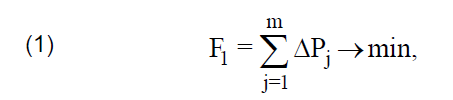
The basic difference between grounding and earthing is that in grounding the conductor through which the current is flowing is connected with the ground while in earthing the conductor through which the current is not flowing is attached with the ground.
In this post, we will have a detailed look at earthing and grounding than relate them to find their differences. So let’s get started with a Difference Between Grounding and Earthing.
Difference Between Grounding and Earthing
Earthing
• Earthing is a process that is used to link the part of the device called the dead portion that has zero value of current with the earth. • The frame of your fridge is a dead part and connects it of the earth • Earthing helps to make a reduction in the getting shock if there is current flowing in the device due to fault. • If earthing is done then current will flow to that part that has less resistance. • For earthing, there is green-colored wire is used • The main purpose of earthing is to save a person from getting shocked by a damaged device that has a current in its body • If someone gets a touch to the body can get shocked if decide is not properly earthed • In case of lighting bouls earthing also saves homes and other apartments • It rescues the fire probability in the different system
Importance of Earthing
The main component of electrical safety is earthing. It entails directly connecting electrical instruments metallic surfaces and exposed conductive portions to the ground. It is mostly used to minimize electric shock and lower the danger of fire from electrical failures.
Earthing in Electrical Systems
When earthing is used in electrical systems, fault currents are ensured to be dissipated and excess voltage is kept from building up on conductive surfaces. By enabling the safe discharge of fault currents into the ground, it helps to prevent electric shock in people.
Components of Earthing
Components like earthing pits, electrodes, conductors, and earthing terminals are used in earthing systems. These components are intended to make a dependable connection configuration with the ground and offer a low-resistance channel for fault currents.
Grounding
• In this process, the active portion of the device means through which the current is passing is linked to the earth. • Its main purpose is to save the device from getting damaged an example is the neutral of the transformer linked to the ground • The main purpose of transform neutral linked to the ground is that if lighting bouts are fallen on it then its grounding will give less resistance path to move to the current to ground • For grounding there is black color wire is used
Importance of Grounding
Electrical engineering’s foundational concept is grounding. It entails attaching electrical devices and systems to the ground or a conductor that acts as a standard for electrical potential. In the case of a failure or surge, grounding primarily serves to offer a safe path for electrical currents to follow.
Grounding in Electrical Systems
In electrical systems, grounding offers a point of reference for voltage levels and helps in system stabilization. By diverting fault currents to the ground and protecting people and instruments from potentially hazardous conditions, it helps in the prevention of electrical shock dangers. With that, grounding decreases electromagnetic interference and guarantees the correct operation of delicate electronic equipment.
Components of Grounding
Grounding systems come with different parts, like conductors, grounding terminals, and grounding connectors. Together, these components make a low-resistance channel for fault currents, helping them to efficiently dissipate into the earth.
Similarities Between Grounding and Earthing
Electrical Safety
By eliminating electrical shock dangers and minimizing the chance possibility of electrical fires, both earthing and grounding help to ensure electrical safety. They offer fault currents paths, providing the safe release of extra energy.
Equipment Protection
Electrical devices can be protected from harm by transient voltages, power surges, and lightning by being grounded and earthed. They decrease the possibility of damage by rerouting fault currents away from the equipment and creating a low-resistance channel to the earth.
Fault Current Management
For successful management of fault currents, both earthing and grounding are needed.. They enable the safe dissipation of fault currents, minimize electrical risks, and decrease the effects of faults on the system as a whole by offering low-impedance routes to the ground.
Grounding vs Earthing
Grounding
Earthing
1. Grounding us the connection if electrical systems to the ground.
1. Earthing is connecting conductive parts and surfaces of electrical equipment to the earth.
2. It provides a path for electrical faults and surges to safely dissipate.
2. It prevents electric shock and decreases the risk of fire.
3. Grounding protects against electrical malfunctions and damage to equipment.
3. Earthing makes sure the safety of individuals and equipment.
4. It stabilizes voltage levels and decreases electromagnetic interference.
4. It discharges fault currents and avoids the buildup of excess voltage.
5. Grounding is necessary for electrical system stability and proper functioning.
5. Earthing is important to make sure electrical safety and prevent accidents.
6. It is get through grounding conductors, rods, and grounding electrodes.
6. It is done through earthing conductors, mats, and earthing electrodes.
7. It is required by electrical codes and standards for safety compliance.
7. It is mandated by regulations to meet safety requirements.
8. It protects against lightning strikes, power surges, and voltage transients.
8. It protects against electric shock and equipment damage.
9. Grounding reduces the risk of electrical noise and interference.
9. Earthing minimizes the risk of electric shock hazards in various settings.
10. It is important in industrial, commercial, and residential electrical installations.
10. Earthing is compulsory in all types of electrical systems and environments.
11. It ensures proper grounding continuity and fault current path.
11. It provides a low-resistance path for fault currents to flow.
12. It prevents static discharge and potential differences in electrical circuits.
12. It prevents the buildup of static electricity and potential differences.
13. This system protects sensitive electronic devices from voltage fluctuations.
13. it protects individuals from electric shock in case of faults.
14. It is important for electrical system safety and the protection of personnel.
14. It decreases the risk of electrical accidents and injuries.
15. it comes with grounding busbars, grounding conductors, and ground fault protection.
15. it involves earthing conductors, grounding electrodes, and earth leakage protection.
16. It maintains electrical system integrity and prevents overvoltage conditions.
16. it maintains a reference potential and prevents electric shock incidents.
17. This process provides a path for fault currents to return to the source safely.
17. This method comes with a safe route for fault currents to flow into the ground.
18. It is important for equipment grounding and protection against electrical faults.
18. it is necessary for equipment safety and minimizing electrical hazards.
19. Grounding is part of a comprehensive electrical safety program and risk management.
19. it forms an integral part of electrical safety strategies and protocols.
20. It ensures the safe operation and longevity of electrical systems and equipment.
20. This techniques ensures the integrity and safety of electrical installations and appliances.
.
Author: Henry, I am a professional engineer and graduate from a reputed engineering university also have experience of working as an engineer in different famous industries. I am also a technical content writer my hobby is to explore new things and share with the world. Through this platform, I am also sharing my professional and technical knowledge to engineering students.
Published by Zia Hameed1, Muhammad Rafay Khan Sial2, Adnan Yousaf3, Muhammad Usman Hashmi, Faculty of Engineering and Technology, Superior University, 17-km off Raiwind Road Lahore Pakistan Emails: zia.hameed@superior.edu.pk, rafay.khan@superior.edu.pk, adnan.yousaf@superior.edu.pk
Abstract—Power System Harmonics is a real point of concern for Electrical Engineers. In power systems, non-linear loads are permanently connected, unlike transients and other distortions are produced. Due to non-linear loads, distortions are produced in the sinusoidal waveform so active shunt filter is used in parallel with the load to minimize these distortions and in a result pure sinusoidal waveform is obtained. Active shunt filter is work as a current source, but opposite in phase sequence to the current which produces by non-linear loads. Harmonics is an all-time problem. Relay protection devices are not good enough to resolve this problem, so other techniques are to be studied to minimize their effects. In this paper my major concern is to identify the loads which causes harmonics, how to design a filter for removing harmonics their effects on power systems, how to design a filter for removing harmonics, proposition of useful filters for altered types of loads and their simulation on ETAP (Electrical Transients and Analysis Program).
Keywords — AC wave, Even Harmonics, Filters, Odd Harmonics, Linear and non-linear loads, ETAP.
I. INTRODUCTION
Service dependability and worth of power have become growing consternations for many capacity directors, especially with the increasing sensitivity of electrical equipment and programmed controls[4]-[6]. There are several types of voltage variations that can cause anomalies, including surges and spikes, sags, harmonic distortion, and temporary disruptions. Harmonics can cause sensitive equipment to failure and other problems, as well as overheating of transformers and wiring, irritation breaker trips, and a bridged power factor[2], [11].
The part of distribution of electric voltages to the power system is very important. This objective is difficult due to Harmonics currents that are produced [9]. They produce harmful effect on the system and disturb its continuity. So when harmonics are produced it is necessary to reduce it for better performance of the system. There are two concepts for which we can understand, how harmonics affect the power system [2], [10]. Firstly, the harmonics are produced due to non-linear loads and the second is that how harmonics current flow and produce harmonic voltage [6].
II. HISTORY
In 1888, Tesla familiarized the concept of poly-phase systems after that in 1890, at Portland, Ore a 1st power transmission line of length 13 miles at frequency of 132 Hz was setup [1], [2]. In the same year, Bedell studied the field of alternating current and also studied the effects of alternating current wave forms in power systems [2], [3]. In 1893, at Hartford engineers dealing with a heating problem of a motor had selected harmonics analysis as a technique to identify the causes of motor heating and tried to solve the problem[3], [4]. Steinmetz discouraged the use of high frequency in power systems because of the high transmission line resonance [6]. It was noticed that the voltage wave form having frequency 133 Hz or 125 Hz was plentiful in harmonics. Steinmetz suggested two solutions for the removal of higher harmonics. First was to reduce the system frequency of 133 Hz or 125 Hz to half i.e. 66.5 Hz or 62.5 Hz. The second suggestion was to refit the iron laminations in the motor which can bear higher in-service voltage [1], [2]. In 1895 generator manufacturing companies Westinghouse and GE presented such generators having distributed armature winding to make the waveform more sinusoidal. It was also noted that when two generators operate in parallel and solidly grounded excessive neutral current flows which causes harmonics. 3rd harmonic was reduced by changing armature winding pitch factor when the neutral of a machine was solidly grounded [3], [5]. In 1910 telephone interference factor was given great importance even in 1980s it was included in the standards due to the large usage of mercury arc rectifier which is a large source of this distortion. In 1960s, in instruction to progress power factor and to reduce the power system harmonics large number of shunt capacitors and filter banks were installed in industrial power systems. In 1812, Jean Fourier developed a mathematical way to analyze the complex functions [1], [2]. This technique expands the complex functions into sine and cosine functions. Harmonics analysis is the name given by Thomson and Tait [1]-[3]. Bernoulli, Euler and Maxwell also used this technique in 18th century. In 1966, J.W Coley and J.W Tuky suggested the Fast Fourier Transform (FFT) as a technique for computer code so that it can give results hurriedly. IEEE standard 519 is now the principle interface standard used by most engineers to judge harmonics issues [3], [4].
III. HARMONIC CONCEPTS
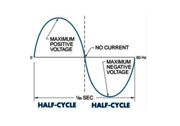
Due to distortion of voltage and current waveform harmonics are produced. Harmonics are mentioned to be a section of a waveform that is the integral multiple of the fundamental frequency. If the load is inserting normal power back to the source at harmonic frequencies, it can be called a Harmonic source.
Fig.1. Odd Harmonics
IV. LINEAR AND NON-LINEAR LOADS
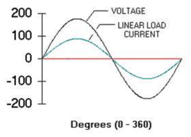
In a power system, current waveform is same as voltage because current is proportional to voltage. Examples of linear loads are heaters and motors.
Fig.2. Linear loads waveform
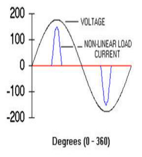
But for Non-linear loads the current and voltage waveform are different. Examples of non-linear loads are UPS and DC motor drives.
Fig.3. Non-linear load wave form
The current waveform is not periodic but it remains same cycle to cycle. Due to sum of sinusoidal waves, periodic waves are generated.
V. VOLTAGE AND CURRENT HARMONICS
The expression ‘harmonics’ is often used by itself without further qualifications. However, the voltage and current harmonics are separate in their effects and are also mutually related. Non-linear loads at the consumer end appear to be injecting the harmonic currents in the power system. For this reason, they are normally treated as harmonic current sources. On the other hand, the harmonic voltages are the result of harmonic current times the linear impedances of the control system. The harmonic current passing through the system resistances causes the voltage drop across it which results in voltage harmonics. Thus, the voltage harmonics are the function of current harmonics and the linear impedances of the power system.
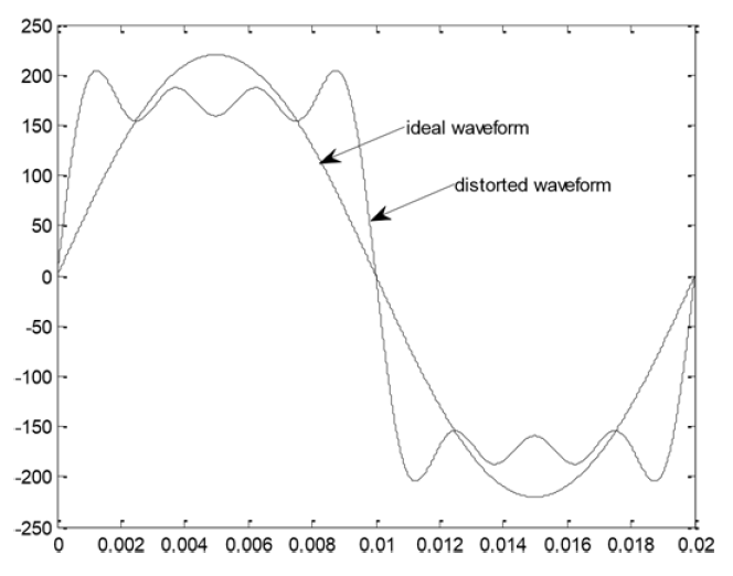
Fig.4 shows a voltage waveform of peak value equal to the secondary distribution level of Pakistan i.e. 220 V. Likewise, it also depicts the harmonics mechanisms with amplitudes of (1/3) to (1/5) and (1/5) to (1/7) of 220V and having the frequencies three, five and seven times the essential frequency correspondingly. Assuming the voltage harmonics are due to the passage of harmonic current through a system resistance.
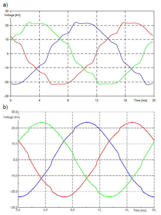
Fig.4. Sinusoidal 50 Hz waveform with 3rd, 5th and 7th Harmonics
Fig.5. Sinusoidal 50 Hz waveform distorted by 3rd, 5th and 7th Harmonics
VI. COMPARISON BETWEEN TRANSIENTS AND HARMONICS
Transients and Harmonics often cause confusion and most of the times one is blamed instead of the other for a particular quality disturbance in power system. The main differences between harmonics and transients are shown in the Table 1.
Table 1: Comparison between Transients and Harmonics
.
VII. EVEN AND ODD HARMONICS
Harmonics are fundamentally the integral multiples of the fundamental frequency. Even harmonics are the even multiples and odd harmonics are odd multiples of the fundamental frequency.
Even harmonics: 2𝑓,4𝑓,6𝑓,…,2𝑛𝑓 Odd harmonics: 3𝑓,5𝑓,7𝑓,…,(2𝑛+1)𝑓 here, 𝑛 is a natural number.
Similar waves contain only odd harmonics but odd and even both harmonics are produced due to asymmetrical waves.
In odd harmonics both positive and negative parts of the wave are same but in asymmetrical waves both positive and negative parts are different. Asymmetrical wave is the result of half wave rectifier.
Control scheme produces only odd harmonics. This is due to same waves. Due to this reason, only odd harmonics will be discussed in upcoming sessions.
VIII. HARMONICS PHASE SEQUENCE
In order to describe a physical three phase system, Power Engineers have adopted a technique of balanced machineries which is based on Fortescue’s theorem. That is stated as:
“An unstable set of 𝑛 phasors may be resolute into (𝑛−1) stable n-phase systems of diverse phase sequence on one zero-phase sequence system.”
Phase sequence of the phasors is the order in which they pass through a positive maximum. A physical 3-phase system with phases A-B-C can be resolved into following three component sets of balanced phasors:
• Positive-sequence contains three sinusoids which are at 120𝑜 from each other. • Negative-sequence contains three sinusoids which are at 120𝑜 from each other and they are opposite to the positive sequence. • Zero-sequence contains three sinusoids that are in-phase with each other.
So for second harmonic, 𝑛=2 we get 2×(0𝑜,−120𝑜,120𝑜) 𝑜𝑟 2×(0𝑜,120𝑜,−120𝑜) It shows negative sequence.
For third harmonic, 𝑛=3 we get 3×(0𝑜,−120𝑜,120𝑜) 𝑜𝑟 (0𝑜,0𝑜,0𝑜), which is the zero sequence. Here is the detail of only odd harmonics:
Harmonics of order 𝑛=3,9,15 … are also named as Triplens. They deserve special consideration because of their critical nature and considerable effects on the behavior of the power system. They are of much importance while discussing grounded-star system containing the neutral current. The two main problems associated with triplens are:
• Overloading of the neutral • Telephone interference
Due to the triplen harmonics, an excessive current flows through the neutral conductor resulting in the overloading of neutral. Among the triplen harmonics, 3rd Harmonic got the much consideration of power engineers.
IX. MEASURING PARAMETERS OF HARMONICS
The result of harmonics is measured by the following methods.
a) Total Harmonics Distortion
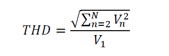
Total Harmonic Distortion is identified by Harmonic Distortion Factor which is the most common technique to calculate harmonics distortion of current and voltage. For an ideal system, THD is equal to zero. THD is determined by:
.
𝑉𝑛 is the rms voltage at harmonic, 𝑁 is the maximum harmonic order and 𝑉1 is the line to neutral rms voltage.
b) Total Demand Distortion
THD can also be applied to study the current distortion stages but in the case of low fundamental load current, it can be deceiving. A small current may carries high THD which is danger for system. For example speed drives shows the high THD values at very light loads for any value of input current. The magnitude of harmonic current is low. This high THD value for input current is not considerable concern even though its comparative distortion to the fundamental frequency is high.
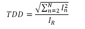
TDD is scientifically calculates:
.
Where 𝐼𝑅 is the peak hours demand load current at the fundamental frequency component determined at point of joint coupling (PCC). There are two ways of calculating 𝐼𝑅. With the load which is already in the system, it can be determined simply by averaging the peak demand current for the preceding 12 months.
X. SOURCES OF HARMONICS
Due to non-linear loads and switching processes harmonics distortion is produced. These sources of waveform can be found in engineering installation in thousands of KVA value. The main sources of harmonics in power system are:
• Due to windings in the transformer and magnetic capacity in stators and rotors of Electrical machines • In the transformer core due to magnetic saturation • Due to rectifiers and inverters • Due to nonlinear loads
A. Rotating Machines
Revolving machines become a source of harmonic distortion because of irregularities in stator and rotor slots or due to winding patterns. So these harmonics produce emf. But these harmonics are very less in quantity as compared to variable speed drives.
B. Transformer
An excessive magnetic flux is produced through the core when transformer operates near the saturation zone. Due to this excessive magnetic flux, linear rise of the magnetic flux density is limited. Core saturation of transformer is resulted when it operates either:
• Above then the rated power • Above then the rated voltage
At rated power harmonics are produced due to peak hour voltages. A Transformer is function on a saturation region so non-linear magnetizing current is found which produces odd harmonics and due to hysteresis losses distortion is produced. Distortion is characteristically due to triplen harmonics, but mostly due to the third harmonic. Delta connection is used to restrict the third harmonic current within the transformer. This helps in preserve a supply voltage with a sensible sinusoidal waveform.
C. Power Electronic Converters
There is a large use of Electronic converters in domestic and industrial purposes due to domestic uses. Single phase rectifier is very common converter which is used for domestic and industrial applications but three phase converter is more danger as compared to single phase converter because it produces 3rd order harmonics which are more dangerous for the power system.
D. Arcing Devices
The foremost harmonic sources in this group are the arc welder’s electric arc furnaces, and discharge type lighting (arc furnace, sodium vapor, florescent) for magnetic (rather than electronic) ballasts. Due to arc furnace in industries, harmonics are produced. So when the arc increases, voltage will decrease in the power system.
E. Future Sources of Harmonics
For Electrical system designer it is a challenge that to design such an instrument for domestic uses and industry that operate at harmonic level. Due to very large use of sensitive electrical and electronic devices harmonics are produced so it is very dangerous in the near future. Due to very large use of switching devices and instruments harmonics are produced which are very dangerous in the near future. Due to distributed generators harmonics are produced specially in peak hours.
XI. EFFECTS OF HARMONICS
Harmonics are very dangerous for the remaining power system and the equipment’s that are attached with the power system. The main effects of voltage and current harmonics within the power system are:
• The possibility of amplification of harmonic levels resulting from series and parallel resonances • Degradation of the power factor • Overheating of the phase and neutral conductors • Efficiency of the generators is reduced day by day due to harmonics • Eddy current and hysteresis losses in transformers • Overheating of the system components e.g. generators, motors and transformers etc. • Flow of additional current through power capacitors • Decrement in the useful lives of the incandescent lamps • Increase skin and proximity effects • Interference problem with telecommunication • Effects the relay protection system
For the adverse effects of harmonics on the power system, it is the major demand of the today’s power system that these harmonics should be mitigated by appropriate designing of the filters either active or passive.
XII. DESIGNING OF FILTERS
Distribution network is a network which is close to the consumers end. Non-Linear loads are attached at the consumer’s end, so mainly Harmonics are produced at the consumers end. So for the removing of Harmonics we used Active shunt filters at the distribution side. Due to non-linear loads reactive current is produced which causes Harmonics. So for removing of reactive current Hysteresis band control method is used to produce trigger signal to the inverter to produce reference current. Due to non-linear loads distortions are produced in the sinusoidal waveform so active shunt filter is used in parallel with the load to minimize these distortions and in a result pure sinusoidal waveform is obtained. Active shunt filter is work as a current source, but opposite in phase sequence to the current which produces by non-linear loads. Similarly filters are also used which work as a voltage source for the removing of Harmonics. When the Harmonics will be removed from the Electrical System then efficiency and life will be increases of the equipment’s. Harmonic current calculator is used for the calculation of Harmonic current, calculator sensed load current and multiply it with unit magnitude of sine and cosine wave, in this way we are able for identify harmonics in the Electrical Power Systems. So Hysteresis bases control circuit is used in the filters for the removing of Harmonics. There are three simulations which are used to filter the Harmonics 1- Simulation of shunt active filter, 2- Simulation of Harmonic current calculator, 3- Simulation of voltage source inverter. But in this paper simulation of shunt active filters is used by using ETAP (Electrical Transient Analyzer Program) software is used. Filters are tuned in such a way that at which frequency they are tuned resonance will be occur and that harmonic content will be filter from the wave.
XIII. ETAP AS A BRILLIANT TOOL FOR HARMONICS ANALYSIS
ETAP is a best tool for the study of harmonics in a power system. With the help of ETAP we can study the Harmonics Analysis of any type of circuit and with the help of ETAP we can also study the Harmonics spectrum. By load flow analysis we can study the harmonics analysis. First of all we study the load flow analysis at the fundamental frequency. With the help of load flow analysis we can study the power factor at different buses in the electrical power system and after that we can check the harmonics analysis and order of harmonic spectrum. By doing the harmonics analysis, low order frequencies are produced.
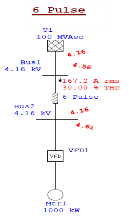
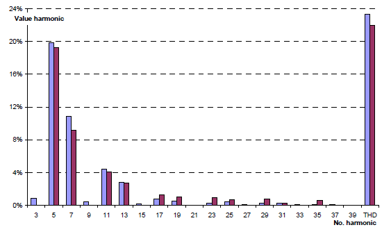
Here we study different cases of “Variable Frequency Drives” using ETAP and observe the effectiveness of this tool.
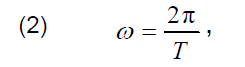
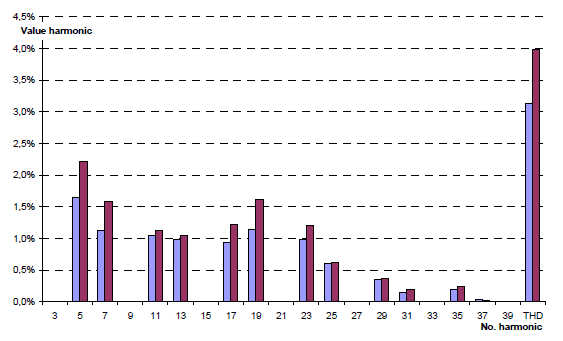
Fig.6. 6-pulse Harmonics Analysis with VFD
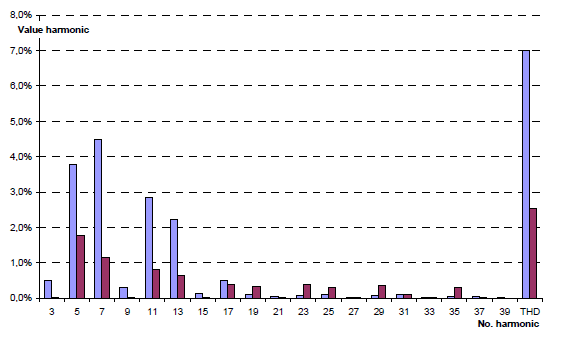
Fig.7. THD with VFD and different Loads.
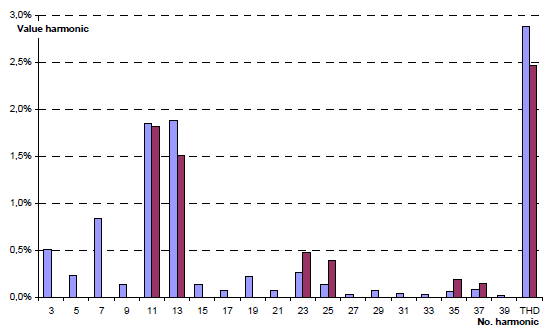
Fig.8. Removing Harmonics of Non-linear by using Filters filters
CONCLUSION
Harmonic distortion is one of the major issues to maintain the power quality. From the results we shown that harmonics are removed by using active shunt filters. Harmonics not only effects the power quality but also cut down the useful life of the power apparatus. It is associated with the major power system components i.e. transformer, synchronous motors, power converter and electrical furnaces. Since these components are continuously connected to the power system, harmonics is all time concern present in the fundamental signal. It is therefore crucial to mitigate this distortion. Harmonics analysis is also very important to study all the effects and the losses which we have to bear. So ETAP (Electrical Transient and Analysis Program) is an important simulation software to check the systems losses and effects before its installation. We conclude that we can check Harmonics Analysis by using ETAP and can be removed by using active shunt filters.
REFERENCES
[1] Edward L. Owen, “A History of Harmonics in Power Systems”, IEEE Industry Application Magazine, Jan/Feb 1998, pp 6-12 [2] P. Berdell,” History of AC wave form, Its determination and standardization”, AIEE, Trans, vol.61, 1942, pp.864-68 [3] S.P. Thompson, “A new Method of Harmonic Analysis by selected ordinate”, Proc. Of the physical society [4] T. R. Bosela, Introduction to Electrical Power System Technology, New Jersey, Prentice Hall, 1997, pp. 458 462. [5] Angelo Baggini, Zbigniew Hanzelka, Handbook of Power Quality, John Wiley and Sons Ltd. England 2008, pp. 187 236. [6] Francisco C. De La Rosa, Harmonics and Power Systems, Distribution Control Systems, Inc. Hazelwood, Missouri, U.S.A. 2006, pp. 1-56. [7] Roger C. Dugan, Mark F. McGranaghan, Surya Santoso, H. Wayne Beaty, Electrical Power Systems Quality, Second Edition, pp. 167 223. [8] R. Rexte, “Power Electronic Polluting Effects”, IEEE Spectrum, May 1997, pp. 33 39. [9] M. Izhar, C. M. Hadzer, S. Masri, S. Idris, “A Study of the Fundamental Principles to Power System Harmonic”, National Power and Energy Conference (PECon) Proceedings, Bangi, Malaysia, 2003. [10] C. Sankaran, Power Quality, CRC Press LLC. [11] John J. Grainger, William D. Stevenson, Power System Analysis, McGraw-Hill Companies, Inc. New York, c1994. pp. 417 418. [12] S. P. Ghosh, A. K. Chakraborty, Network Analysis and Synthesis, McGraw-Hill Education, c2010, pp. 933. [13] S. L. Clark, P. Famouri, W. L. Cooley, “Elimination of Supply Harmonics”, IEEE Ind. Appl. Magazine, March 1997. [14] E. B. Makram, R. B. Haines, A. A. Girgis, “Effect of Harmonic Distortion in Reactive Power Measurement”, IEEE Trans. Ind. App., vol. 28, no. 4, July 1992. [15] Control of Harmonics in Electrical Power Systems, American Bureau of Shipping, May 2006, pp. 29 48. [16] L. Cividino, “Power Factor, Harmonic Distortion; Causes, Effects and Considerations”, IEEE Telecommunications Energy Conference INTELEC 92, 14th International, Oct. 1992, pp. 506 513. [17] Jos Arrillaga, Bruce C. Smith, Neville R. Watson, Alan R. Wood, Power System Harmonic Analysis, University of Canterbury, Christchurch, New Zealand, pp. 7 25. [18] W. M. Grady, R. J. Gilleskie, “Harmonics and how they relate to Power Factor”, IEEE San Diego, Nov. 1993, pp. 1 8. [19] IEEE Harmonics Modeling and Simulation Taskforce, “Modeling and simulation of the propagation of harmonics in electric power networks part I”, IEEE Trans on power delivery, vol.11, no. 1 , Jan 1996, pp.466-474. [20] A. Median, “Harmonic simulation techniques (Methods and Algorithms)” IEEE Power Engineering Society General Meeting , Vol.1 , June 2004, pp.762-765 [21] Pravin Chopade and Dr. Marwan Bikdash, “Minimizing Cost and Power loss by optimal placement of capacitor using ETAP”, IEEE 2011 pp.24-3
Author: Zia Hameed was born in 1991 in Bahawalpur, Pakistan. He is doing his Graduation in Electrical Power Engineering from The Islamia University of Bahawalpur (2010-14). He contributed his part in this project work especially in the sources and effects of Harmonics. He also played a major role in the study of Filters. He complete different Electrical courses from best worldwide universities like MIT, Delft institute, University of Toronto. Currently he is serving as a Lab Engineer at Electrical Engineering Department of Superior University, Lahore. Contact: +92-343-7177273 Email: zia.hameed@superior.edu.pk
Published by Jakub KELLNER1, Michal PRAZENICA2, Department of Mechatroncs and Electronics, Faculty of Electrical and Information Technology, University of Zilina, Slovakia
Abstract. This article deals with the problem of elimination inrush currents. The document proposes an active method for limiting the inrush currents during circuit switching when high inrush currents occur. The proposed system limits current in the circuit by means of a series connected Mosfet transistor. The Mosfet transistor is controlled in a linear resistive region. In the case of an inrush current in a circuit, the Mosfet transistor limits the magnitude of the current flowing into the circuit. The article also solves the problem of transistor power load. In the article there is a chapter that deals with the maximum magnitude of the limiting current that can flow through the transistor so as not to destroy it. In this new inrush current limiting configuration, the operator can directly define the amount of surge current that must not be exceeded after the circuit is closed. The proposed system is also complemented by other protective and control elements that are described in this article.
Streszczenie. Artykuł dotyczy problemu eliminacji prądów rozruchowych. Zaproponowano aktywną metodę ograniczania prądów rozruchowych podczas przełączania obwodu, gdy występują duże prądy rozruchowe. Proponowany system ogranicza prąd w obwodzie za pomocą szeregowo połączonego tranzystora Mosfet. Tranzystor Mosfet jest kontrolowany w liniowym obszarze rezystancyjnym. W przypadku prądu rozruchowego w obwodzie tranzystor Mosfet ogranicza wielkość prądu wpływającego do obwodu. Artykuł rozwiązuje również problem obciążenia mocy tranzystora. W artykule jest rozdział poświęcony maksymalnej wielkości prądu ograniczającego, który może przepływać przez tranzystor, aby go nie zniszczyć. W tej nowej konfiguracji ograniczania prądu rozruchowego operator może bezpośrednio określić wielkość prądu udarowego, której nie wolno przekroczyć po zamknięciu obwodu. Proponowany system uzupełniono również innymi elementami ochronnymi i kontrolnymi opisanymi w tym artykule. Eliminacja nadmiernego wzrostu prądu rozruchowego
With increasing demands on the power of electric motors for various technical sectors (e.g. electric vehicles for traction purposes), the power of power semiconductor converters for connecting these motors is also increasing. As the power of the inverters increases, there is a problem with the inrush current. The problem of inrush current is compounded when using traction battery power used in cars.
The inrush current is the instantaneous input current of a high amplitude circuit that occurs when the circuit is switched on as a result of charging capacitors, inductors and transformers. This inrush current has a large amplitude and can reach currents of up to several tens of kilo-ampere [1] – [4].
Fig. 1 Current curve when the circuit is switching on (inrush current)
Therefore, it is very undesirable in electrical circuits. In circuits where the inrush current occurs, the elimination of this undesirable phenomenon is solved by increasing the resistance in the circuit. In most cases, a resistor or an NTC thermistor is used to increase the resistance in the circuit. The duration of the inrush currents is of the order of milliseconds, the duration of this action being dependent on the size of the RC members in the circuit. Figure 1 shows an example of the current waveform when in the circuit the inrush current was generated [5] – [8].
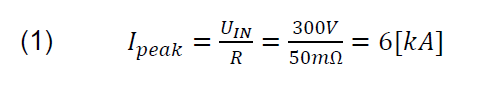
The system designed by us solves the elimination of surge currents for the 9kW inverter, which is used to power supply the asynchronous motor. Input voltage for the inverter is realized by traction batteries with nominal voltage 300V, DC. The total charge capacity in the circuit is 5mF and the parasitic resistance in the circuit is estimated at 50mΩ. In this case, the inrush current would occur during the power on the Ipeak = 6kA circuit. This is confirmed by the simulation shown in Figure 2. Since the capacitor at the moment of switching on was a short circuit, the current was limited only by the resistance in the circuit:
.
Fig. 2 Simulation of inrush current in the circuit, without limitation
Due to the high inrush current, it is not suitable to use a resistor or an NTC thermistor for limitation. Therefore, we decided to design a system that uses a controlled Mosfet transistor. The advantage of this system is that we can adjust the magnitude of the inrush current. This system can also be used for other circuits that have lower voltage and current parameters for which this system was designed [9].
Inrush current limitation with Mosfet transistor
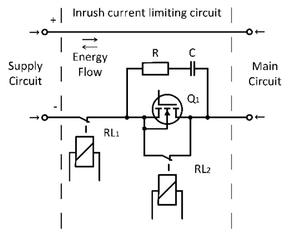
As mentioned above, the inrush current during the initial start-up of the inverter that feeds the asynchronous motor can be limited by the Mosfet transistor. A schematic diagram of this circuit is shown in Figure 3.
Fig. 3 A schematic diagram of the system
By controlling the transistor in its resistive area, we can reduce the magnitude of the inrush current generated by the charging of the capacitors of the inverter. This method is much more efficient and preferable than using a resistor or NTC thermistor. The advantages of this configuration are:
1.) Possibility to set maximum surge current. The user can set the amount of current which must not be exceeded. This feature allows the designed system to be used for other applications where inrush current limitation is required [10] – [12].
2.) System efficiency. Because it is a power semiconductor converter, we try to make the converter efficiency as high as possible. Therefore, the use of a resistor is not appropriate. We would reduce the efficiency of the inverter. But if we use a Mosfet transistor, we can effectively regulate the power supplied to the DC bus inverter [13].
3.) Power load of the limiting component. If we used a Resistor to limit the current, the power dissipation at the resistor would be too high.
Example of calculating instantaneous power on the limiting resistor (Pdissipation), for the proposed application: Supply voltage: UIN = 300V, DC; Circuit Capacity: C = 5mF; Limiting resistance: R = 20Ω. The effective value of the current in the circuit was: Irms = 5,9A. Power dissipation is [14]:
.
Power part design
Figure 4 shows a schematic of the power section of the inrush current limiting system. The power part of the proposed system consists of three main parts. These are active power semiconductor components. The main semiconductor component that provides the whole principle of inrush current limitation is Mosfet transistor. Its control ensures the limitation of the current flow in the circuit. The transistor is active in the case of over currents that occur during circuit switching on. Another element in the circuit is relay 2, which serves as a bypass member.
Fig. 4 Power part of the system
Relay 2 is connected in parallel to the transistor and at the moment the inrush current limitation is complete, relay 2 closes and the transistor is bypassed. The third active element in the power section is relay 1, which ensures the overall start and stop of the system. It also serves as a protective relay.
In the power section, an RC snubber is also contemplated to optimize the transistor to avoid failure during operation. The system can conduct current in both directions. Therefore, it is suitable for use in traction applications where we can measure and adjust the amount of current flow.
Simulation results of the proposed system
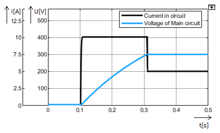
The proposed system was simulated in Matlab / Simulink environment. The simulation is based on current limitation during the initial inverter switching on. At this point, high capacity is charging. Figure 5 shows the voltage on the main circuit and the current flowing into the circuit. Using a current limiting transistor, we regulated the current in the circuit to I = 10A. Where we suppressed the current from 6kA to 10A. This, however, greatly increased the delay time τ.
Fig. 5 Simulation of inrush current limitation
Figure 6 shows the waveforms that determine the operation of the transistor and bypass relay.
Fig. 6 Conductivity waveforms of transistor and bypass relay
The black waveform shows the current on the transistor that limits the inrush current to 10A. The orange waveform represents the voltage across the transistor, which gradually decreases, while the voltage across the main circuit increases. The green curve represents the current through the bypass relay. We can see that if the voltage on the transistor drops to zero, the voltage on the main circuit will be equal to the supply voltage. Then the transistor turns off and the bypass relay is turned on, through which the load current flows into the circuit.
Simulation verification of transistor power load
This chapter shows the results of the transistor power load during the current limitation. In the simulation for the limitation, we detected the power losses on the Mosfet transistor at the time the transistor was in operation using the “Pe_getPowerLossSummary” function [15] – [17].
Table 1 shows the Mosfet current through the transistor, the time delay, the power dissipation on the transistor, and the energy on the transistor. The simulation input voltage is UIN = 300V. Main circuit capacity is C = 5mF.
Table 1. Transistor load simulation varication
.
For the measured loads and time delays, we created a graph of the magnitude of the current through the Mosfet transistor, which can be seen in Figure 7. From the waveform we can see that with increasing current the delay time decreased but the power load of the transistor increased periodically.
Fig. 7 A waveform to determine the maximum permissible current limiting through a transistor
Using this function, we can determine the maximum current limiting magnitude for a selected Mosfet transistor so that it does not exceed its maximum permissible power load. To prevent Mosfet transistor from straining.
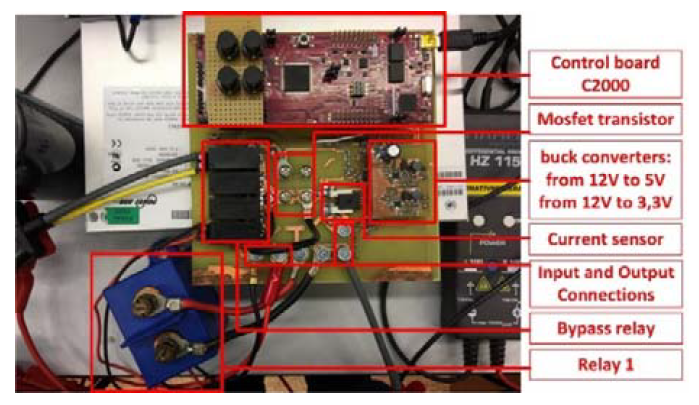
Fig. 8 Real sample of proposed system
System verification on real sample
The proposed system was verified on a real sample. Measurements were performed at reduced parameters. The prototype was created for the experimental verification of system functionality. The thickness of roads and conductive connections of real sample does not correspond to the power load for which the system was designed. Therefore, all experimental measurements were verified at reduced voltage. Figure 8 shows a prototype of the proposed system. The illustration shows the description of each part of the system. The designed system was controlled by a C2000 microcontroller from Texas Instrument TMS 320F28069. Figure 9 shows the waveforms from the inrush current limitation measurement. The inrush current is limited to Ilim = 3,6A. The main circuit capacity is C = 4,2 mF. Supply voltage is UIN = 37V.
We can see from the waveform that the current in the circuit did not exceed the allowed current during charging.
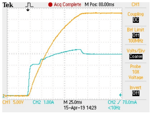
Fig. 9 Inrush current limitation measurement
The yellow waveform represents the voltage on the main circuit. The blue waveform represents the current in the circuit. The main circuit was gradually charged to the supply circuit voltage. After the capacitor was charged, the current in the circuit remained at I = 4A. Because the main circuit was loaded with a resistance R = 9,2Ω. The time delay in the circuit was 120ms.
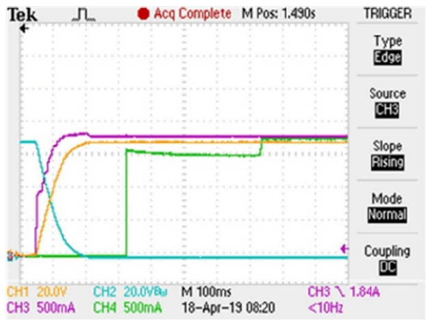
Figure 10 shows the waveforms of inrush current limitation of a main circuit with the following parameters: UIN = 70,5V; Rload = 39Ω; C = 2,2mF. The yellow waveform represents the voltage on the main circuit, which gradually increased to the value of the supply voltage. The blue waveform represents the voltage on the transistor. This, in turn, drops to zero. The purple waveform is the current in the circuit. The current was limited to Ilim = 1,8A. The load current in the circuit is Iload = 1,7A. The green curve represents the current through the bypass relay. From this we can see that the transistor led the current during the inrush current limitation. Then the transistor and the relay led simultaneously. And then only the bypass relay conducts current to the load.
Fig. 10 Measurement of main circuit inrush current limitation
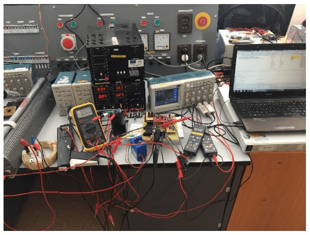
Figure 11 shows a measurement workstation consisting of a power supply, current probes, oscilloscope, multimeter, voltage probes, load resistance, load inductance, auxiliary power supplies and a notebook for communication with the microprocessor.
Fig. 11 Measuring workplace
Conclusion
This article presents a new design of the inrush current limiting system. It is an effective way of limiting. In the proposed system there is the possibility to specify the magnitude of the maximum inrush current. Therefore, the system can be used for various applications. Current limitation is solved with Mosfet transistor, which provides considerable advantages over conventional methods of limiting inrush current. The proposed system was verified by simulation and on a real sample. Results from simulations and measurements are presented in this article. From the results we can see that the proposed system successfully limits the magnitude of the inrush current during the initial switching on of the main circuit.
Acknowledgement This work was supported by projects: Vega 1/119/18 Research of the methodology for optimization of EMC of WPT systems, ITMS 26210120021.
LITERATURA
[1] J-Ch. Wu, H-L. Jou, K-D Wu, N-T Shen, Hybrid Switch to Suppress the Inrush Current of AC Power Capacitor, IEEE Transaction on Power Delivery, vol. 20, n. 1, pp. 506-511. [2] T. Jiang, P. Cairoli, R. Rodrigues, Y. Du, (2017). Inrush current limiting for solid state devices using NTC resistor. SoutheastCon 2017. doi:10.1109/secon.2017.7925398. [3] Iuga, B., & Tirnovan, R. A. (2019). Step by step Limiting for Capacitors Inrush Current Used in Voltage Power Supplies. 2019 8th International Conference on Modern Power Systems (MPS). doi:10.1109/mps.2019.8759664. [4] H. Suryoatmojo, M. Ridwan, I. Izzatur Rahman, D. Candra Riawan, M. Ashari, Design of Bidirectional DC-DC Cuk Converter for Testing Characteristics of Lead-Acid Battery, Przeglad Elektrotechniczny, doi:10.15199/48.2020.03.26. [5] R. Araria, K. Negadi, M. Boudiaf, F. Marignetti, Non-Linear Control of DC-DC Converters for Batery Power Management in Electric Vehicle Application, Przeglad Elektrotechniczny, doi:10.15199/48.2020.03.20. [6] G. Mallesham, K. Anand, Inrush Current Control of a DC/DC Converter Using MOSFET, International Conference on Power Electronic, Drives and Energy Systems 2006, India. [7] K. Praveen, N. Kulshrestha, L. Srivani, D. Thirugnanamurthy, B. K. Panigrahi, Prognostics of Electrolytic Capacitors under Inrush Current Overstress, International Conference on Smart City and Emerging Technology (ICSCET) 2018, India. [8] Eun-Ju Lee, Jung-Hoon Ahn, Seung-Min Shin, Byoung-Kuk Lee, Comparative analysis of active inrush current limiter for high-voltage DC power supply system, 2012 IEEE Vehicle Power and Propulsion Conference. [9] M. Frivaldsky, P. Špánik, J, Morgos, M, Pridala, Control strategy proposal for modular architecture of power supply utilizing LCCT converter, Energies, Vol. 11, N. 12, 2018, Article Number: 3327. [10] Gonthier, L., & Renard, B. (2015). AC/DC reversible mixed inverter with built-in inrush-current limitation and cut-off standby losses. 2015 17th European Conference on Power Electronics and Applications (EPE’15 ECCE-Europe). doi:10.1109/epe.2015.7309066. [11] K. Dabala, M. P. Kazmierkowski, Converter-Fed Electric Vehicle (Car) Drives, Przeglad Elektrotechniczny, doi:10.15199/48.2019.09.01. [12] M. Frivaldsky, J, Morgos, B. Hanko, Start-up power supply for automotive applications, International Conference Elektro 2018, CZ. [13] Madani, S. M., Rostami, M., Gharehpetian, G. B., & Haghmaram, R. (2012). Inrush current limiter based on threephase diode bridge for Y-yg transformers. IET Electric Power Applications, 6(6), 345. doi:10.1049/iet-epa.2011.0317. [14] H. Hoshi, T. Tanaka, M. Noritake, T. Ushirokawa, K. Hirose, M. Mino, Consideration of Inrush Current on DC Distribution System, Proceedings of Intelec 2012, USA. [15] J.K. Kim, S. S. Lee, W-S. Oh, J-E. Kim, G-W. Moon, Ch-H. Gil, J-R. Cho, Start- up inrush current reduction technique of asymmetrical half-bridge DC/DC converterfor PC power supply, 7th Internatonal Conference on Power Electronics, 2007, South Korea. [16] J. Sedo, S Kascak, Control of single-phase grid connected inverter system, International Conference Elektro 2016, Slovakia. [17] B. Dominikowski, Inteligentne pomiary szybkozmiennego prądu akumulatora trakcyjnego pojazdu elektrycznego wykorzystujące interwałowe zbiory rozmyte typu-2 o wnioskowaniu Takagi-Sugeno-Kanga, Przeglad Elektrotechniczny, doi:10.15199/48.2019.11.12.
Authors: Ing. Jakub Kellner was born in 1995 in Kezmarok, Slovakia. He is graduated at the University of Zilina (2019) in Power Electronics. He is currently an internal PhD student at the University of Zilina – Department of Mechatronics and Electronics in the power electrical engineering study program. The main research interest is about power electronic systems.
Ing. Michal Prazenica, PhD was born in 1985 in Zilina, Slovakia. He is graduated at the University of Zilina (2009). He received the Ph.D. degree in Power Electronics from the same university in 2012. He is now Research worker at the Department of Mechatronics and Electronics at the Faculty of Electrical Engineering, University of Zilina. His research interest includes analysis and modelling of power electronic systems, electrical machines, electric drives, and control.
Source & Publisher Item Identifier: PRZEGLĄD ELEKTROTECHNICZNY, ISSN 0033-2097, R. 96 NR 8/2020. doi:10.15199/48.2020.08.20
Published by Shivanand M N1, Y. Maruthi1 Phaneendra Babu Bobba2, Sandeep Vuddanti1 1GRIET, EEE Department, Hyderabad, Telangana, India 2CUK, Electrical Engineering Department, Kalburgi, Karnataka, India *Corresponding author: shivanandnaduvin@gmail.com
Abstract. India has taken major step in adopting the electric vehicle by means of FAME Scheme (Fast Adoption and Manufacturing of Electric Vehicles), a government initiative. ARAI (Automotive Research Authority of India) and DHI (Department of Heavy Industry) have published standardization protocol for both EV charging infrastructure. Many of those standards are derived from the SAE (Society of Automotive Engineers) Internationals and IEC (International Electrotechnical Commission). USA, Europe and China are also following the same standards to build the EV (Electric Vehicle) infrastructure. This paper provides the Indian standards to build EV charging infrastructure and comparing it with other countries. Glimpses on energy demand for electric vehicles in Indian market. It also provides the demanding wireless power transfer technology in EV’s. Status of Standards provided by the industry on wireless power transfer. Factors that are necessary to be considered before drafting the standards for WPT.
1 India’s Charging Infrastructure
India aims to have at least 15 percent of the vehicles on its roads to be electric in five years, signalling the government’s wish to join a long list of countries around the world that are already seeking to cut fossil fuels aggressively. While cumulative global sales of passenger electric vehicles likely surpassed 4 million in August, with China accounting for more than a third since 2011, India sold an estimated 2,000 EVs 2017. EVs may account for about 7 percent of sales in India by 2030 by [1]. The government of India (Department of Heavy Industries – DHI) is already providing incentives through FAME scheme (Faster Adoption and Manufacturing of Electric Vehicles) from the year 2015 in order to reduce the price of EV’s. The government has also approved pilot projects, charging infrastructure projects and technological development projects. Energy Efficiency Services Limited (EESL), under the administration of Ministry of Power, Government of India (GoI), has ordered 10,000 EVs [2]. With all the initiation that India has been taking, there is serious issue of charging infrastructure for both wired and wireless charging system. Standardization to the technical aspects of the EVs charging, range and price are the major barrier for deployment. Currently in India, there are very small scale of AC and DC charging stations available, which are installed by EV manufacturers. Even though the AC slow charging infrastructure at residences, workplaces and public places requires very low investment when compared to fuel stations. Still, the EV charging infrastructure growth in India is not up to the mark. To grow large scale of charging infrastructure in India it requires continuous support from the government, utility grid authorities and automobiles manufacturers.
1.1 Indian EV Charging Standards
Department of Heavy Industry (DHI) & Automotive Research Association of India (ARAI) drafted industry standard for Electric Vehicle Charging infrastructure on December 2015. The first draft of AC-charging configurations are Type-I and Type-II. Type-III standards are published in the second draft on May 2017. [3]
1.1.1 Type-I: AC001(3.3KW,15A,230V)
● Derived from IEC 60309 Standard ● AC Slow charging ● Each outlet will have up to three independent charging sockets. ● Input: 3 phase AC Supply, 5 wire (3 phase+ Neutral +PE- Protective Earth). Nominal Input Voltage is 415V (+6% and -10%) as per IS 12360 ● Frequency is 50Hz ± 1.5 Hz ● Output: Single phase, two wire system 230V (+6% or -10%) and 15 Amps as per IS12360 ● No Communication protocol is used between EV and EVSE (EV Supply Equipment)
1.1.2 Type-II: AC001(>3.3KW)
● Charger power is greater than 3.3KW. ● This AC Fast charging. ● Outlet is derived from the Standard IEC 62196 and IEC 61851. ● Charging with 415V, three phases, 63A. ● Control Pilot (communication protocol) extends to control EV charging Equipment system (EVSE).
1.1.3 Type-III: DC001(48V/2V,10KW/15KW)
● Input: 3 phase AC Supply, 5 wire (3phases+N+PE). Nominal Input Voltage is 415V & frequency is 50Hz ± 1.5 Hz (+6% and -10%) Maximum 200 Amps as per IS 12360. ● Output- 48V or 72V DC, based on suitable charger Configuration for vehicle battery. ● Charger Configuration Types ● Single Vehicle charging at 48V/72V with a maximum of 10kW, or a 2 Wheel vehicle charging at 48V with maximum 3.3kW. ● Single Vehicle charging at 48V with a maximum of 10KW, or 72V with maximum 15kW or a 2 Wheel vehicle charging at 48V with maximum 3.3kW.
1.2 Charging System Available in The World
1.2.1 The International Electrotechnical Commission (IEC 62196) modes definition:
Mode-1: Slow charging from a regular electrical socket (single or three phase) Mode-2: Slow charging from a regular socket but which equipped with some EV specific protection arrangement Mode-3: Slow or Fast charger using a specific EV multi-Pin Socket with control and protection functions Mode-4: Fast charging using some specific charger technology such as CHAdeMO. [4]
1.2.2 European EV Standards
● Normal power or Slow Charging with rated power inferior to 3.7kW is used for domestic application or for long-time EV parking. ● Medium power or quick charging with a rated power from 3.7-22kW is used for private and public EV ● High power or fast charging with a rated power superior to 22kW is used for public EV [4]
1.2.3 American EV Standards
TYPE-1: The charger is on-board and provides an AC voltage at 120 or 240 volts with a maximum current of 15A and a maximum power of 3.3kW
TYPE-2: The charger is on-board and provides an AC voltage at 240V with a maximum current of 60A and a maximum power of 14.4kW.
TYPE-3: The charger is off-board, so the charging station provides DC voltage directly to the battery via DC connector with maximum power of 240kW. [4]
Table 1. Electrical Rating of Different Charge Method in North-America
.
1.2.4 EV charging based on Power and Usage Location
Charging ratings of different electric vehicles based on their usage are classified from normal power rating of 3.7kW to >22kW.
Table 2. Classification of EV charging based on Power and Usage Location.
.
2 Electric Vehicles in India
2.1 Energy Demand for EV
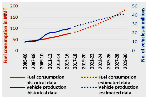
Energy required by utility grid increases as demand in the electric vehicle market. The automobiles production in India is at a CAGR of 5.81% from 2007 to 2018. The vehicles include 80.9% of two wheelers, 13.2% of passenger cars, 2.5% of three wheelers & 3.4% of commercial vehicles [5]. Out of these, close to 99.9% are conventional ICE vehicles which are burning petrol & diesel for traction. The figure 1 shows the historical vehicle production data along with the estimated production volumes by 2030 which is indicated with blue line and also it shows the historical & estimated fuel (both petrol & diesel) consumption in MMT (Million Metric Tonnes) which is indicated with red line.
Fig. 1 Fuel Consumption & Vehicle Production Data
The total electricity generation in India during the year 2016-17 is 1160TWh which is used in domestic, commercial, industrial & agriculture sectors. The total electricity required, if all the existing ICE vehicles are converted into BEV’s during the year 2016-17 is 439TWh which is 34.26% additional to the existing electricity generation. By 2030, the electricity generation (Egen) in India will grow along with the demand in the domestic, commercial, industrial & agriculture sectors which is shown in the figure 3 (indicated with blue). Apart from this, there will be a growth in the production of automobiles in India by 2030 and if all these vehicles are 100% BEV’s the required electricity generation (Egen_tr) demand on the utility grid increases which is also shown in the figure 3 (indicated with red).
Fig. 2 Projected Electricity demand up to 2030
Hence by 2030 in India, 100% of BEV’s would require an energy of 929.3 TWh which is about 37% additional electricity to be produced apart from estimated electricity generation of 2500 TWh (includes domestic, commercial, agriculture & industrial sectors etc.) [6].
2.2 Indian Automobile Industry – An Overview
The Indian Automobile Industry is currently ranked 5th largest in the world and is set to be the 3rd largest by 2030.The requirement of mobility in India is set to change dramatically in the near future to cater to the requirement of 1.30 billion population While there is a vision for 100% electric vehicles by 2030, most industry experts indicate that around 40-45% EV conversion by 2030 is a realistic expectation. A major push towards EVs will be led by the public transportation requirements in India – Fleet cars, E-Buses, 3 wheelers and 2 wheelers. Personal vehicle options for EVs will still be a relatively smaller element in the whole pie. The Government plans to work towards creating a demand for EVs by buying in bulk, which could provide for large orders for automakers. A tender for 10,000 cars is already issued and now a major tender for electric buses in 11 cities is likely to be released soon. [7]
2.3 The outlook for 2018
– Passenger cars to see a higher increase in new model launches compared to utility vehicles.
-Production capacity will also be added at car makers to reduce waiting periods and to boost demand. (Passenger vehicle segment growing between 7-9%).
– In the two-wheeler segment, motorcycles are expected to grow moderately while scooters will continue to grow in double digits with two-wheelers growing between 9-11% in FY’18.
– Industry moving towards a March 2020 launch of BS-6 and most OEM/Auto component firms have made investments to meet this deadline.
2.4 EV Chargers
2.4.1 EV Chargers in India
Post FAME and the Niti Ayog Plan announcement, we have seen an increased trust on setting up EV chargers in India. Some names we could confirm, who have joined interest in EV Chargers manufacturing are Raychem RPG India, Analogic India, Deltron, EOS Power, AdorPowertron, Kraft Power Con, Elind etc.
2.4.2 Global EV Charger firms on Indian Market
More than six key global firms eyeing the EV Chargers market closely. Firms like ABB India, Delta India, Schneider India, Siemens India etc are looking at the Indian market closely. These firms have their global designs and products. They are studying the technical/specifications, business models and potential for their products. All these firms are only looking at the 4 Wheelers’ (Cars) EV Chargers.
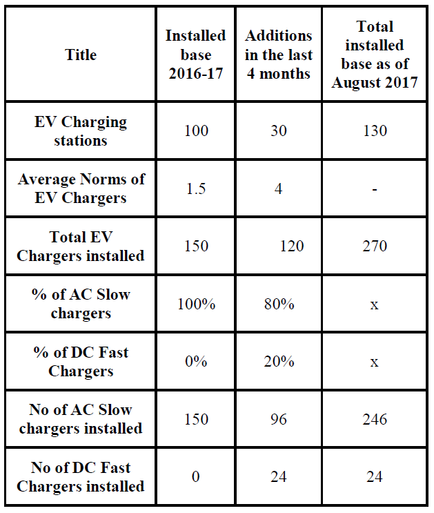
Table 3. Total number of EV Charging Stations in India
.
Table 4. Likely future market for EV Chargers in India
.
3 EV Wireless Charging Standards
As the world is advancing towards the wireless charging from smaller biomedical application to the electric vehicle charging system. Standardization is the main barrier holding the commercialization of high-voltage and high-power WPT for EV charging. It includes safety criteria, efficiency, EM(Electromagnetic) limits, and interoperability targets, along with test setup for getting wireless charging. It should provide the compatible charging station to all the EV owners. IEC-61980-1 standard contains the total system of WPT from supply network to EVs charging the battery or any equipment of the same at the standard supply of 1000-Vac or 1500-Vdc. These all are addressed by SAE in its standard SAE TIR J2954 (TIR-Technical Information Report). This is the first standard developed by SAE in WPT for an EV charging application. This standard is developed specifically for SWC. The frequency band, interoperability, safety, coil definitions, and EMC/EMF limits from SAE TIR J2954 allow any attuned vehicle to charge wirelessly from its wireless home charger, office or a commercial charger with the same charging ability. Table 5 shows key standards for wireless charging. [8] In the near term, vehicles that are capable to be charged wirelessly under recommended practice should also be able to be charged by SAE J1772 plug in chargers. SAE recommended practice J2954 is intended to be used for stationary applications (charging while vehicle is not in motion). Dynamic applications may be considered in the future based on industry feedback. SAE Recommended Practice J2954 is meant to be used for interoperability, performance and emissions testing, where a single standard coil-set has been chosen for the WPT Power Class 1 and 2 to 7.7kW, per Z-Classes (1 through 3) which is circular topology. However, there are two reference options for WPT 3 to 11kW per Z-classes (1 through 3) with two topologies. The next revision of the Recommended Practice in 2018 is slated to have one standard coil set for WPT 3. SAE TIR J2954 establishes a common frequency band using 85 kHz (81.39 – 90 kHz) for all light duty vehicle systems. [9].
Table 5. Wireless Charging standards
.
4 CONCLUSION AND FUTURE WORK
The major obstacle to the adaptation wireless EV’s charging is the standardization. The inductive coupled power transfer has given greater results than the other types of system. The factors that needs standardization are geometry of coils, volume and weight, position of coil, alignment, frequency, compensation topologies, distance and Efficiency. Including the human and environmental consideration due to electromagnetic radiation. DHI and ARAI has provided standards for conductive charging infrastructure. The standards provided are very limited to the charging equipment and its features. But lacks in charging time, driving range, lack of awareness and efficiency.
Published by Huimin Wang1, and Zhaojun Li2, 1School of mechanical and electrical engineering University of Electronic Science and Technology of China Chengdu, China. Email: hmwang1206@163.com 2Department of Industrial Engineering and Engineering Management Western New England University, Springfield, MA, 01106. Email: zhaojun.li@wne.edu
Abstract—The failure of power system transient stability is one of the main factors causing catastrophic accidents of power systems. Therefore, it is of great significance to evaluate the transient stability of a power system. This paper first introduces the evaluation methods of power system transient stability, including the assessment methods based on time domain simulation, direct method, artificial intelligence-based methods and the probabilistic assessment method. The key challenges in power system transient stability assessment are reviewed and analyzed, including the stability evaluation of power-electronized power system and the main elements of artificial intelligence method used in transient stability assessment. Last, the future research directions and conclusions are discussed.
Keywords – transient stability assessment; power system; power-electronized power system; probability assessment; artificial intelligence
I. INTRODUCTION
Power system transient stability is that the ability of generators to continue to operate synchronously after the system is disturbed [1]. The causes of failure of power system transient stability include short-circuit fault, sudden disconnection of lines or generator, etc. Accurate and fast transient stability assessment method is important to the security operation of power system. With the gradual advancement of smart grid construction, long-distance, huge capacity transmission mode and high-proportion power electronics, the new risks are introduced in power system [2]. Power shortage accidents and complex cascading failures further rise the difficulty of power system stability analysis and control.
The direct method, time domain simulation method and artificial intelligence (AI) method are commonly used for transient stability analysis of traditional power system [3].
The time domain simulation method is to solve the differential equations and algebraic equations, which describe the transient process of the system by various numerical integration methods. Then the stability is judged according to the change of the relative angle between the rotor of the generator. In each step interval, it is approximated that the rotor is in constant acceleration motion [4].
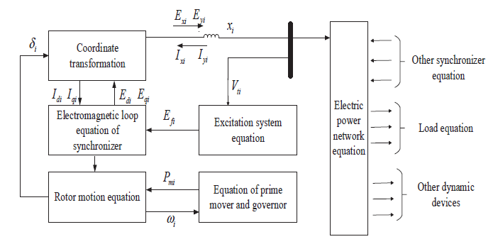
The direct method is mainly based on Lyapunov stability criterion, which is proposed by constructing a function directly in order to quantitatively measure the power system transient stability [5]. Traditional transient stability calculation is carried out under the condition that the topology, parameters, operation conditions and disturbance modes of power system are given. The structure of power system network model is presented in Figure 1.
Figure 1. The model structure of power system whole network
In Figure 1, Idi and Iqiare rotor current of direct-axis and quadrature-axis respectively; Ediand Eqi are rotor voltage of direct-axis and quadrature-axis; δi is power angle; Exi and Eyi are stator voltage of direct-axis and quadrature-axis; Ixi and Iyi are stator current of direct-axis and quadrature-axis; Efi is excitation voltage; Vtiis node voltage; Pmiis input power of prime mover; wiis angular speed of prime mover.
However, previous works focused on the application of different methods to establish Lyapunov functions for power systems. With the development of Lyapunov functions, it is recognized that another key problem is to accurately estimate the stability region after failure of power systems [6]. The calculations of energy function of flexible AC transmission system (FACTS) devices and revised transient energy function of FACTS are formulated in [7].
With the advantage of wide-area measurement system (WAMS) technology, the artificial intelligence prediction method based on WAMS can use real-time measurement data to train the transient stability classifier online, instead of using off-line model to simulate various disturbances to obtain data [8]. Artificial intelligence generates databases as input of established networks through a large number of off-line simulations, and uses intelligent algorithms to construct stable classifiers. Then the stability of the system is evaluated by training stable classifiers [9]. The method of Artificial intelligence is used to develop a load disaggregation approach for bulk supply points based on the substation rms measurement in [10]. The optimization problem is formulated, and the Cuckoo search algorithm is adopted for optimal designing of power system stabilizer in [11]. The analysis about artificial intelligence optimum plans and improving the functioning of the power systems economically are made in [12]. Compared with the time domain method, the artificial intelligence method does not need to establish the mathematical model of the power system. Artificial intelligence method uses the measured response information to extract the characteristics that can reflect the physical nature of the system transient stability. Then the transient stability assessment is carried out by establishing the mapping relationship between the characteristics and the system stability.
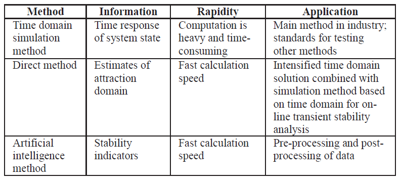
Usually, artificial intelligence takes an offline approach to obtain feature samples which can accurately characterize the inherent mechanism of power system operation under anticipated accidents. The acquired samples are trained and learnt repeatedly, and the method of predicting the transient stability of power system is constructing the classifier. Meanwhile, the feature samples are input into the classifier in real time. The comparison of the three methods for evaluating the power system transient stability is shown in Table I.
TABLE I. COMPARISONS OF THREE METHODS
.
II. BASIC ANALYSIS STEPS OF DIFFERENT METHODS APPLIED TO TRANSIENT STABILITY ANALYSIS
A. Time Domain Simulation Method for Transient Stability
From the previous discussion, the calculation of traditional transient stability is carried out under the condition that the topology, parameters, operation conditions and disturbance modes of power system are given. The time domain simulation method is to solve the differential equations and algebraic equations, which describe the transient process of the system by various numerical integration methods. The equations are as follows:
.
where δ is angle of power energy; w is angular frequency; wN is rated angular frequency; TJis electromagnetic torque; PT is mechanical power and Pe is electromagnetic power.
B. Direct Method for Transient Stability
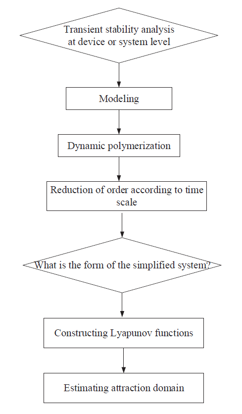
The direct method is mainly based on Lyapunov stability criterion. The direct method contains potential energy boundary surface (PEBS), relevant unstable equilibrium point (RUEP) and extended equal area criterion (EEAC) [13]. The EEAC method refers to that the regulation of excitation can also promote the transient stability of power systems [14]. A multi-objective optimization method is proposed, which is to model transient stability as an objective function rather than an inequality constraint in [15]. Only the excitation system with fast rise of excitation voltage and high peak voltage can have a significant effect on improving transient stability. The reason is that fast excitation reduces the acceleration area, increases the deceleration area and then improves the transient stability of the system. Good excitation control plays a more important role in increasing artificial damping and eliminating the second pendulum or multi-pendulum out-of-step [16]. Basic steps of direct method are shown in Figure 2.
Figure 2. Basic steps of direct method
C. Probabilistic Assessment for Transient Stability
Some parameters of power system are random due to errors in measurement, estimation or calculation [17]. The operating conditions and random disturbances are ever-changing, and deterministic analysis does not consider the possibility of various accidents. Transient stability probability analysis is different from deterministic analysis [18]. Different from deterministic analysis, the transient stability probability analysis determines the probability indicators according to the statistical characteristics of the main stochastic factors affecting power system transient stability.
Considering the power system, tcr and tcl are assumed to be the critical and actual clearing times of the fault respectively. The principle of calculating the probability indicators of transient instability is shown in Figure 3 [19,20].
Figure 3. The principle of calculating the probability indicators of transient instability
If and only if tcl > tcr, the system will be transient unstable. The fault clearing time tcl is a random variable, and the system transient stability assessment can be expressed by the probability of system instability when the fault occurs.
.
In the formula, I refer to the event leading to transient instability of the system and the probability density function of the fault clearing time is tcl. If tcr and probability density function of the fault are known, it is easy to obtain the probability indicators of transient instability of the system under this fault condition.
In summary, the method of probabilistic transient stability analysis of power system is divided into analytical method and Monte Carlo method [21]. In order to assessing the probability of power system stability, the conditional probability theory is used. The influence of probability distribution of random factors is mainly considered. Comparison of flow charts of deterministic and probabilistic of transient stability analysis of power system is shown in Figure 4.
The analytical method uses conditional probability theory in statistics to evaluate the stability probability of the system. The probability indicators of transient stability are determined according to the statistical characteristics of the factors that will affect the power system transient stability. Probabilistic transient stability analysis makes up for the limitation of deterministic method in transient stability analysis, which is an important breakthrough and supplement to deterministic method.
Figure 4. Comparison of flow charts of deterministic and probabilistic power system transient stability analysis
But the calculation of probabilistic transient stability analysis is usually very large. Probabilistic analysis of transient stability of power system involves the probability of the system state, which depends not only on the location and type of the fault, but also on the relay protection settings, and the system state before the fault. The probabilistic transient stability analysis procedures are shown in Figure 5.
Usually, disturbance accident simulation is that using probability model to simulate disturbance accident, disturbance includes location, type and other information.
In the process of Monte Carlo simulation, some uncertain parameter models can be obtained from historical data or assumed to be a probability distribution function. The probabilistic transient stability assessment includes state sampling, transient stability simulation and transient instability indicators calculation. Probability assessment of transient stability of power system based on Monte Carlo method is shown in Figure 6.
Figure 6. The assessment of transient stability of power system based on Monte Carlo method
D. Artificial Intelligence Method
Artificial intelligence method is applied to on-line transient stability analysis. Input feature selection and evaluation model are the key points in the research of assessment of transient stability of power system based on artificial intelligence.
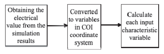
In the construction of assessment of transient stability strategy based on artificial intelligence, the stable discriminant input characteristic is composed of some combined operational variables reflecting the dynamic response during system failure. Subsequently, artificial intelligent technologies are applied to establish the relationship of the input characteristics and the stable state of transient stability characteristics. In the process of modeling, choosing appropriate input features is the key to design, and the electrical value should be converted in center of inertial (COI) frame. A large number of studies have applied feature transformation algorithms such as injection principal component analysis to reduce the input feature dimension and improve learning efficiency [22]. The basic steps of obtaining input characteristic variables are shown in Figure 7.
Figure 7. The basic steps of obtaining input characteristic variables
III. TRANSIENT STABILITY ASSESSMENT OF POWER ELECTRONIC DOMINATED POWER SYSTEM
A. Power Electronics Dominated Power System
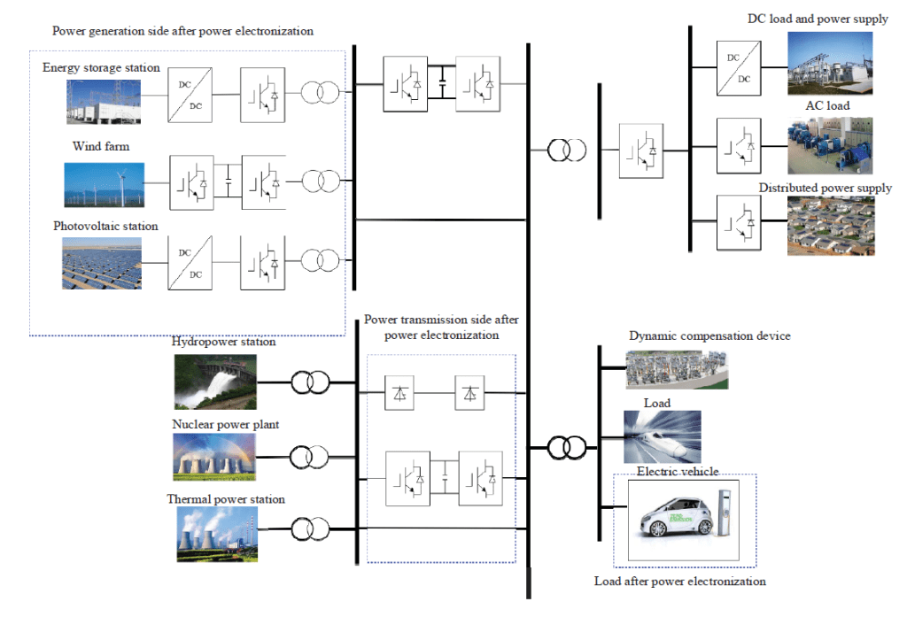
With the rapid development of new semiconductor materials and control technology, the penetration of power electronic converter in power supply side, transmission network and load side of power system is getting higher and higher, and the power level of power electronic converter is also rising. Since the 1950s, power semiconductor technology has made great progress. Converters are formed to connect to power systems as voltage or current sources [23]. The power-electronized power system is presented in Figure 8.
Compared with traditional AC power system, the characteristic of power-electronized power system is that the system topology changes with the switching action of power electronic devices. The whole system is time-varying (nonautonomous), and there is interaction of multi-time scale control. In addition, the power electronic converter itself has structural nonlinearity and complexity, and there are overmodulation and limiting phenomena when using pulse width modulation. So that the power electronics dominated power system has saturation nonlinearity. These characteristics bring difficulties to power system stability analysis [24]. The stability of power electronic dominated power system was determined by time domain method, impedance analysis method and generalized short circuit ratio previously. At present, the small signal stability analysis of power-electronized power system has achieved preliminary results. Small signal stability can ensure the asymptotic stability of the equilibrium point, which is a necessary step in device design. However, considering small signal stability alone, the boundary of the stability region can not to be determined and the stability margin of the equilibrium point can not to be judged. Therefore, it is needed to analyze the transient stability of power electronics dominated power system.
B. Artificial Intelligence Method for Transient Stability Assessment of Power Electronics Dominated Power System
Time domain simulation method is considered to be the most mature and reliable method, which is also applicable to power electronic power system. However, the simulation method has the disadvantages of large amount of calculation, long simulation time and impossible to simulate all operation states.
Another main method of transient stability analysis which can be used in power-electronized power systems is that direct method based on modern differential dynamic system. The direct method determines the transient stability of the system by comparing the transient energy with the critical energy of the power system at the time of fault clearing.
However, conventional algorithms of stability analysis and the stability control systems is unable to evaluate the power system operation under smaller and smaller stability margin. Thus, the AI method are complementary to the traditional transient stability analysis method. Artificial intelligence method is applied to on-line transient stability analysis.
Figure 8. Power electronics dominated power system
Artificial intelligence method is mainly used in combination with wide area monitoring system, which undertakes the functions of pretreatment and post-processing. Transient stability assessment is a mapping from characteristic information to stability category. Its basis is to determine the classification step of decision attribute. Eight attribute variables are listed in the Table II. The class variables are stable and unstable, which are expressed by 1 and 0 respectively.
TABLE II. COMPOSITION OF ATTRIBUTE VALUE OF INPUT VECTOR
.
There are many characteristics reflecting transient stability. One of the purposes of classifier design is to select representative conditional attributes variables, in order to provide as much information as possible by using conditional attributes. Some features related to transient stability can be extracted. Machine learning algorithm is applied to assessment of transient stability, the key problems including initial feature input, feature selection, model learning and training. The difficulty lies in obtaining the characteristic sample set which can represent the physical essential characteristics and designing the classifier with the lowest error rate for transient stability assessment. The transient stability assessment process of power electronics dominated power system is shown in Figure 9.
IV. DISCUSSION ON FUTURE TRENDS
Figure 9. The assessment of transient stability of power system
The artificial intelligence method can realize the identification and decision-making of fast determination of power system transient stability, which is based on the measured data rather than the power system model and parameters. However, this method does not take into account the physical mechanism of the dynamic response of the power system, and requires precise learning samples when calculating. However, it is difficult to provide a large number of valid samples matching the actual operation through off-line simulation. Therefore, artificial intelligence method applied to power system transient stability has the difficulties including deep mining of massive WAMS data, off-line simulation and errors in the use of measured data.
In addition to the traditional power system analysis method, a new analysis method of power system transient stability should be proposed according to the characteristics of power electronics dominated power system. The analysis method combined with bifurcation theory can be studied.
In the aspect of data acquisition, simulation method is used to obtain transient stability analysis data instead of relying on actual fault data. The main reason is that the probability of actual power system failure, especially transient instability, is low. Because the power system vary with time, the applicability of historical data decreases and it is difficult to provide high-quality training data for artificial intelligence algorithm. From this point of view, how to improve the consistency between simulation data and actual fault data is an urgent challenge to be solved.
V. CONCLUSION
This paper presents an overview of the power system transient stability assessment methods. A comprehensive analysis and comparison of the deterministic assessment and probabilistic assessment is presented. Compared with traditional AC power system, the characteristics of power electronics dominated power system have changed dramatically, but it is essentially still a time-varying and nonlinear complex system. The characteristics of power-electronized power system are analyzed, and the artificial intelligence methods of transient stability for power-electronized power system have been presented. In addition, the AI methods which have been used to analyze power system transient stability are reviewed, and data acquisition, feature extraction and algorithm application are discussed.
This research is partially supported by the National Science Foundation of China, No. 71771038.
REFERENCES
[1] P. Kundur, N. J. Balu, and M. G. Lauby, Power system stability and control, New York: McGraw-hill, 1994. pp.30-46. [2] F. Li, W. Qiao, H. Sun, et al. “Smart transmission grid: Vision and framework,” IEEE Trans. on Smart Grid, vol. 1, pp. 168-177, February 2010. [3] M. Pavella, “Power system transient stability assessment-traditional vs modern methods,” Control Engineering Practice, pp. 1233-1246, October 1998. [4] M. L. Crow, Computational methods for electric power systems, Crc Press, 2015. [5] J. Geeganage, U. D. Annakkage, T. Weekes, et al. “Application of energy-based power system features for dynamic security assessment,” IEEE Trans. on Power Systems, vol. 30, pp. 1957-1965, April 2015. [6] T. L. Vu, K. Turitsyn, “Lyapunov functions family approach to transient stability assessment,” IEEE Trans. on Power Systems, vol. 31, pp. 1269-1277, February 2016. [7] J. Aghaei, M. Zarei, M. Asban, et al. “Determining potential stability enhancements of flexible AC transmission system devices using corrected transient energy function,” IET Generation, Transmission & Distribution, vol. 10, pp. 470-476, February 2016. [8] S. M. Ashraf, A. Gupta, D. K. Choudhary, et al. “Voltage stability monitoring of power systems using reduced network and artificial neural network,” International Journal of Electrical Power & Energy Systems, vol. 87, pp. 43-51, 2017. [9] K. W. Kow, Y. W. Wong, R. K. Rajkumar, et al. “A review on performance of artificial intelligence and conventional method in mitigating PV grid-tied related power quality events,” Renewable and Sustainable Energy Reviews, vol. 56, pp. 334-346, 2016. [10] Y. Xu, J. V. Milanović, “Artificial-intelligence-based methodology for load disaggregation at bulk supply point,” IEEE Trans. on Power Systems, vol. 30, pp. 795-803, February 2015. [11] S. M. A. Elazim, E. S. Ali, “Optimal power system stabilizers design via cuckoo search algorithm,” International Journal of Electrical Power & Energy Systems, vol. 75, pp. 99-107, 2016. [12] S. M. Zahraee, M. K. Assadi, R. Saidur, “Application of artificial intelligence methods for hybrid energy system optimization,” Renewable and Sustainable Energy Reviews, vol. 66, pp. 617-630, 2016. [13] S. C. Savulescu, Real-time stability in power systems: techniques for early detection of the risk of blackout, New York: Springer, 2006. pp. 147-165. [14] B. Wang, B. Fang, Y. Wang, et al. “Power system transient stability assessment based on big data and the core vector machine,” IEEE Trans. on Smart Grid, vol. 7, pp. 2561-2570, May 2016. [15] C. J. Ye, M. X. Huang, “Multi-objective optimal power flow considering transient stability based on parallel NSGA-II,” IEEE Trans. on Power Systems, vol. 30, pp. 857-866, February 2015. [16] Y. Zhou, H. Huang, Z. Xu, et al. “Wide-area measurement system-based transient excitation boosting control to improve power system transient stability,” IET Generation, Transmission & Distribution, vol. 9, pp. 845-854, September 2015. [17] M. Panteli, D. N. Trakas, P. Mancarella, et al. “Boosting the power grid resilience to extreme weather events using defensive islanding,” IEEE Trans on Smart Grid, vol. 7, pp. 2913-2922, June 2016. [18] C. Peng, J. Zhang, “Delay-distribution-dependent load frequency control of power systems with probabilistic interval delays,” IEEE Trans. on Power Systems, vol. 31, pp. 3309-3317, April 2016. [19] M. Vatani, T. Amraee, A. M. Ranjbar, et al. “Relay logic for islanding detection in active distribution systems,” IET Generation, Transmission & Distribution, vol. 9, pp. 1254-1263, December 2015. [20] T. Gonen, Electrical power transmission system engineering: analysis and design, CRC press, 2015, pp. 300-328. [21] S. Liu, P. X. Liu, X. Wang, “Stochastic small-signal stability analysis of grid-connected photovoltaic systems,” IEEE Trans. on Industrial Electronics, vol. 63, pp. 1027-1038, February 2016. [22] K. P. Wong, “Artificial intelligence and neural network applications in power systems,” International Conference on Advances in Power System Control, pp. 37-46, 1993. [23] Q. C. Zhong, “Power-electronics-enabled autonomous power systems: Architecture and technical routes,” IEEE Trans. on Industrial Electronics, vol. 64, pp. 5907-5918, July 2017. [24] Y. Yang, H. Wang, A. Sangwongwanich, et al. Design for reliability of power electronic systems, Power Electronics Handbook. Butterworth-Heinemann, 2018, pp. 1423-1440.
Published by Sivaraman P, SMIEEE, PEng (India), Senior Power Systems Engineer Chennai, Tamil Nadu, India
We all know that Total Harmonic Distortion (THD) and Total Demand Distortion (TDD) are used to evaluate the presence of harmonics in the power system.
The “IEEE Std 1547-2018 IEEE Standard for Interconnection and Interoperability of Distributed Energy Resources with Associated Electric Power Systems Interfaces” and “IEEE Std 2800–2022 IEEE Standard for Interconnection and Interoperability of Inverter-Based Resources (IBRs) Interconnecting with Associated Transmission Electric Power Systems” provides another terminology called “Total Rated Harmonic Distortion (TRD)” for evaluating the presence of current harmonics in the Inverter Based Resources (IBR) plant or renewable power plants.
As per IEEE Std 1547-2018, TRD is defined as the total root-sum-square of the current distortion components (including harmonics and inter-harmonics) created by the DER unit expressed as a percentage of the DER rated current capacity (Irated).
As per IEEE Std 2800–2022, the non-fundamental frequency RMS current flowing (including harmonics, interharmonics, and noise) between the transmission system (TS) and the inverter-based resource (IBR) plant with respect to the rated RMS current capacity (Irated).
As per IEEE Std 1547-2018, the TRD can be calculated by using the below expression,
.
Where,
• I1 is the fundamental current as measured at the RPA • Irated is the DER rated current capacity (transformed to the RPA when a transformer exists between the DER unit and the RPA) • Irms is the root-mean-square of the DER current, inclusive of all frequency components, as measured at the RPA
As per IEEE Std 2800-2022, the TRD can be calculated by using the below expression,
.
Where,
• I1 is the fundamental-frequency current as measured at the RPA • Irated is the IBR plant rated current capacity based on IBR plant MVA rating at the RPA • Irms is the root-mean-square of the IBR plant current, inclusive of all frequency components up to 50th order, as measured at the RPA; measurement of harmonics to the 50th order requires meters compliant to IEC 61000-4-30 Class A
Note: RPA – Reference Point of Applicability. RPA shall be Point of Common Coupling (PCC) or any other location
Author: Sivaraman P, SMIEEE, PEng (India), Senior Power Systems Engineer Chennai, Tamil Nadu, India. LinkedIn Profile
Published by Somudeep Bhattacharjee1, Saima Batool2, Champa Nandi1 and Udsanee Pakdeetrakulwong3,* , 1Tripura University, 2School of Information Systems, Curtin Business School, Curtin University, 3Nakhon Pathom Rajabhat University *Corresponding author; e-mail: udsanee@webmail.npru.ac.th
Abstract. Selecting the location for installing electric vehicles charging stations is important to ensure EV adoption and also to address some of the inherent risks such as battery cost and degradation, economic risks, lack of charging infrastructure, risky maintenance of EVs, problems of its integration in smart grid, range anxiety, auxiliary loads and motorist attitude. In this article, we investigate these problems by studying three aspects – 1) three types of electrical vehicle charging stations (Level 1, Level 2 and DC), 2) different types of batteries and 3) different types of electric vehicles. We compared and contrasted the features of these charging stations, batteries and EV to identify the best choice for a given scenario. We applied the framework proposed in [1], and used Agartala, India as a case study to identify location for charging stations in and around Agartala suburbs.
Keywords: Electric vehicle, charging stations, electric vehicle battery, charging stations location conditions, infrastructure
1. Introduction
An electric car is actually an alternative-design automobile that basically uses an electric motor to provide power to the car, with the electricity being provided by a battery. On the other hand, a conventional car does have a lead-acid battery as part of its standard equipment but this battery is used for operating the starter and not providing power to the vehicle. This technology works in this way that the electric vehicle uses a motor just like conventional, internal combustion engine cars. The main difference is that the electric vehicle power supply is derived from its battery-stored electricity and not from the mechanical power derived from burning gasoline. The electric vehicle replaces the traditional gasoline or diesel engine and fuel tank with an electric motor, a battery pack and controllers. The vehicle uses a controller that provides power to the electric motor that uses rechargeable batteries as its energy source. The motor itself can be either AC or DC. The main advantage of electric vehicle is mainly the motor and battery configuration. This allows the vehicle to run more fuel efficiently. PHEV (plug in hybrid electrical vehicle) is a hybrid vehicle that can be plugged into the power grid for charging the battery. In this vehicle, a medium-capacity battery is available that helps the electrical vehicle in allowing it in all-electric modes , to achieve several kilometers , and acceleration rates and also it help to attain top speeds comparable to those of gasoline-powered vehicles. Examples: Chevrolet Volt (often classified as an EREV), Ford C-Max and Fusion Energi, Cadillac ELR and Toyota Prius PHEV. On the basis of different types of power trains (or drive trains), hybrid electric vehicles can be classified into three categories:
(1) Parallel hybrid, (2) Series hybrid, and (3) Power-split hybrid.
Among these, the parallel hybrid electric vehicle is commonly adopted. PHEVs are usually consists of an electric motor and an additional ICE for propulsion. This mixed propulsion system helps in enabling PHEVs to be driven in two modes: charge depleting (CD) mode and charge sustaining (CS) mode. When this type of electric vehicles operated in CD mode then it mainly drawn energy from on-board battery packs. If the battery state of charge (SOC) has been depleted to a pre- determined level, PHEVs will then switch to CS mode and utilize the ICE system for further propulsion. When it is operated in CS mode, PHEVs combine both power sources so that it can operate as efficiently as possible. Meanwhile, the controller can monitor the battery SOC level and then maintain it with in a pre- determined band.
2. Objectives
Global warming is becoming a major problem and the best way to combat it is to reduce air pollution. Electric vehicles (EVs) are considered a best option to reduce air pollution and making environment safe again. In order to operate, electric vehicles need charging stations at suitable places. If appropriate and recommended places are not chosen then it will decrease the utilization, visibility and effectiveness of a charging station, which results in adoption of traditional carbon- emitting gasoline vehicles and a decrease in EV sales. Hence, it is very essential to carefully select locations for EV charging stations for promotion of EVs and the cause of avoiding global warming.
The main objective of this study is to determine the best locations for installing EV public charging stations in Agartala, India. Our selection for EV charging station location will depend on the set of conditions that have to be met in order to qualify for a place to be established as an EV public charging station. In addition, we will also determine the best type of charging station based on the type and charging duration of the particular EV type. Finally, this research will provide a specific and thorough insight of establishing EV public charging station in growing cities like Agartala, India.
3. Research Methodology
The framework proposed by [1], is used as a guideline to assess the implementation of EV charging infrastructure for Agartala city. To achieve this, 3 areas are studied 1) Different types of charging stations, 2) EV types, 3) battery types. First of all, different types of charging stations are studied and compared. Next, various types of EVs are analyzed thoroughly. Moreover, the charging vehicle location selection conditions, infrastructure and the best suitable places in Agartala are selected based on the electric vehicle charging station location selection conditions and the map of Agartala.
Preliminary Concepts
We know that as the global benefits of a serious energy crisis, alternative energy for sustainable development is renewable energy .The generation of this energy is pollution free and so this is the first choice of many countries of the world like the United states, Japan and Europe and so the development of electric vehicles is a way to save nature and to resolve important issue of planning the national grid. An electrical vehicle requires charging station and so the locations of charging station have to be determined carefully. A charging station is a location where an electric vehicle can be plugged in to have electric charge deposited in to their batteries. They are not chargers, but can be considered as an electrical energy source.
Different types of charging stations:
There are mainly three types of charging stations which are categorized as Level 1, Level 2 and DC charging stations.
LEVEL 1 Charging Station (120 volts and up to 16 amps): In all electrical vehicles, an on-board Level 1 charger is equipped that can be plugged into any normal power outlet (C S A 5-15R*). It gives an advantage of not requiring any electrical work, or at least minimizes any installation costs. Table 1 shows the charging time using a Level 1 charger based on distance driven. 12-A charging cable and 120-V outlet is considered. Charging cable rated less than 12A require longer charging times [3].
LEVEL 2 Charging Station (240 volts and 12-80 amps): In this type, the charging time of Level 2 charging stations can be limited by the specifications of the on-board charger and the state of the battery, irrespective of the rated power of the charging station. It is believed that the charger capacity is going to increase in future, for example, Tesla already offers on-board 10 kW and 20 kW chargers. Table 1 shows that level 2 charging stations takes less time to charge as compared to the level 1 charging stations even though the distance traveled is similar. Level 2 charging stations have smart and timeless design. It is simple to use (plug the EV in and let it charge). It helps in reducing energy consumption. In addition, it offers Ethernet network for Radio Frequency Identification (RFI) authorization and vehicle ground monitoring circuit. The cord holder keeps the cord organized and out of the way of parking spaces, sidewalks and streets, etc. One example of this is Schneider EV link Indoor Charging Station, which has ground monitor and user friendly LEDs to display status like charging, detected fault, power etc. It has the capability for automatic recovery and restart after ground fault interrupt or main power loss [1].
DC Fast Charging Station (480 volts and up to 125 amps):
DC fast-charge stations generally support two standards: The North American SAEJ 1772 Combo standard and the Japanese JEVS G105-1993* standard. The configuration of the charging plug and the electrical vehicle socket follows the same basic principle compared to the communication protocol between the charging station and the electrical vehicle but have different standards [1]. Table 1 shows the time required to charge a battery with a 100-km range to 80% of its full capacity.
Analysis of Different Charging Stations
Table 1 shows the comparison of different charging stations which are categorized as Level 1, Level 2 and DC charging stations based on electric vehicle distance travelled in km, estimated energy consumption of electric vehicle in kWh, charging station power of electric vehicle in kW, approximate charging time in hour.
Table 1: The comparison between different charging stations levels (Adopted from [1]
.
Why Level 2 charging station is more suitable?
The answer to this question lies in this fact that the most important condition for selecting an electric vehicle charging station location is that how much time is spend by the consumer for charging his vehicle in the charging station. So the time spend is an important factor.
From these charts, it is clear that for the same amount of distance travelled in km, electric vehicle required different charging time in each type of charging station. Also it is shown that Level 2 charging station provides facility to consumer to charge his vehicle in a very short time as compared to other types of charging station. The charts that are shown above prove this.
Types of Electric Vehicles (EVs)
EVs can be divided into the following categories. First, on-road highway speed vehicle that is an electrical vehicle capable of driving on all public roads and highways. The performance of these electrical vehicles is similar to Internal Combustion Engine vehicles. Second, the city electric vehicles, normally, the city electric vehicles have been BEVs (Battery Electric Vehicle – these vehicles can be powered 100% by the battery energy storage system available on-board the vehicle) that are capable of driving on most public roads, but basically not driven on highways. The maximum speed is typically limited to 55 mph. Third category of EVs is also known as low speed vehicles (LSVs). Actually they are BEVs that are limited to 25 mph and are allowed in certain jurisdictions to operate on public streets posted at 35 mph or less. Commercial On-Road Highway Speed Vehicles is the last category of EVs. The commercial electric vehicles include commercial trucks and buses. These vehicles are available in both BEVs and PHEVs (Plug-in Hybrid Electric Vehicle – the vehicles utilizing a battery and an internal combustion engine (ICE) which is powered by either gasoline or diesel). Table 2 provides information on several different on-road highway speed electric vehicles, their battery pack size, and charge times at different power levels to replenish a depleted battery.
Table 2: Different types of EVs with battery pack size and charging times at different power levels (Adopted from [1])
.
Note: Power delivered to battery is calculated as follows: 110VAC x 12Amps x.85 eff.; 110VAC x 16Amps x .85 eff.; 220VAC x 32 Amps x.85 eff.; 480VAC x √3 x 85 Amps x .85 eff. From Table 2, it is clear that different electric vehicle configuration require different charging time for different battery size at different power levels to replenish a depleted battery. This helps to find out the charging time in minutes required by different electric vehicle configurations of different battery size at different power levels. Using Table 3, we study the charging time for 100km of BEV range with power supply, power (in kW), voltage (in V) and maximum current (in A). It helps to show the relation of charging time of fixed 100km distance with its power supply, power (in kW), voltage (in V) and maximum current (in A). Thus, the driver finds charging an electric vehicle as simple as connecting a normal electrical appliance. In addition, Table 12 provides comparison between different recharge times of BEV for 100km range. Consequently, it seems clear that charging through single phase takes longer time then 10 minutes of direct current charging, that is the reason for advocating for DC charging infrastructure for EVs.
Table 3: Charging time for BEV range of Electric Vehicles (Adopted from [1])
.
ELECTRIC VEHICLE BATTERY
The electric vehicle battery is the core component of an electric vehicle with one of the two propulsion sources of HEV and PHEV. Basically, the battery is the sole propulsion source for BEV. There are still some constraints on present EV battery technology, which works as a barrier for wider EV uptake. The current EV battery has relatively low energy density. This low energy density directly affects the maximum all-electric drive range of the EV. In addition, high battery cost of EV is also a big disadvantage as the purchase cost of EV is considerably higher than conventional internal combustion engine vehicle. Some concerns are also present about the battery life cycle and its safety features. However, EV battery goes through some tremendous improvements in the past decades. EV battery technology goes through a few development phases for inventing the battery with highenergy density, high power density, inexpensive, safe and durable. Lead-acid battery was the initial battery technology used in transportation and its name comes from the combination of lead electrodes and acid used to generate electricity. Lead-acid battery is a really a matured technology and also cheap. However, some apparent drawbacks of lead-acid battery are present, such as low energy density, heavy, require inspection of electrolyte level and are not environmentally friendly.
Table 4: Comparison of EV Battery Types and their specifications (Adopted from [3])
.
Table 5: Comparison of EV Battery Types and their specifications (Adopted from [3])
.
Charging Vehicle Location Selection
The sites of the charging station have a very significant impact loads, at this point, charging station is very similar to traditional gas station, charging station requires a higher penetration of electric vehicles in areas surrounding the construction of a natural high, such as new urban planning to support key enter prices and so on. Our work contributes to identify suitable locations for construction of public charging stations. In this paper we have analyzed possibilities of establishing a public EV charging station in Agartala, India in particular. Charging stations located along the highways are also in high demand since high speed EVs usually requires fast charging.
Public Charging Stations
In this section we will list and describe the most suitable charging locations for the installation of public charging stations. These charging stations can be located at parking lots that serve train stations, shopping centres, restaurants, hotels and resorts. When selecting a potential charging station, the following criteria should be considered.
Traffic density
The first criterion is traffic density. Traffic density is a necessary factor because the size of the installation should be related to be expected number of users. If the charging station is located near a major road, with high traffic density, then maximum number of people may use it for charging their electrical vehicles. However, areas with high traffic density are in densely populated locations, where the land value is significantly higher. One way to address this concern is to use land that is already allocated for traditional parking lots and convert them to EVSPLs (Electric vehicles solar parking lots) [4]. Further, these lots can also be converted to multi-level parking’s where the EV can be on the top where they receive sunlight whereas the traditional vehicles can be underneath.
EV Charging Duration
The second criterion is EV charging duration; i.e. how long does it take to charge an electric vehicle. Electric vehicle need time to charge so it is necessary that the charging stations should be located near public places like shopping centres, work places, educational institutions so that people do not have to wait while their EVs are charging. The charging can happen while they are doing their usual activity such as being at work, weekly shopping etc. As (Nunes et al., 2016) suggests that public charging stations should be installed on worksites and public parks. This allows EV users to charge their EVs without having to wait [4].
Surrounding Vehicle Movement
The third criterion is the surrounding vehicle movement. This is important because charging vehicles must not hinder normal traffic flow, as it will become a hurdle, which may even cause accidents. Further, this location must not hinder pedestrian traffic or be subject to high pedestrian traffic because of the associated risk of vandalism. Public EV charging stations have numerous effects on its surrounding environment, transportation and energy needs and hence these implications have to be examined carefully [4]. One way of implementation would be along the street side parking bays. Electric vehicles (EV) have a very diverse characteristic, as it can act both as consumer and producer. In first case, EV’s act as consumer, it is depended on renewable energy resources, batteries, smart grid (G2V- Grid to vehicle) and electric chargers to recharge. In second case, it is producer as well, as EVs can be an essential part of the smart grid. It can act as an energy producer since it stores energy and can provide it back to smart grid when the demand is at peak, this process is known as discharge or (V2G- vehicle to grid). Whereas, there are some concerns about customers’ behaviour in participating in V2G programs that is uncertainty about their participation. Describing the solar panels on parking panels and its impacts on energy in the surrounding areas, it is evident that parking lots are a lot more visible and hence can attract potential customers for electric vehicles making EV adoption much more easier [4]. Consequently, EV adoption can have significant positive impacts on human health [4]. Another impact of solar parking lots is their benefit to local market. Since customers will choose a shopping centre with solar parking lots because it will charge their cars while they do their shopping. This will boost the local economy [4]. In addition, there will be lots of employment opportunities for the local technicians to install and maintain a solar parking lot [4]. Hence, installing a solar parking lot is beneficial in a number ways for a particular location like Agartala, India and its surrounding areas.
Winter Accessibility
The fourth criterion is winter accessibility. The location must be cleared and accessible during winter since some countries have severe winters [1]. The use of EVs should not depend on weather and hence EV public charging stations should be available at all times. Photovoltaic covered EV charging stations protect it from severe weather conditions like condensation, freezing rain and frost etc. [5].
Protection from Collisions
The fifth criterion is protection from collisions. The location must provide protection against collisions. It is necessary to provide protection for avoiding accidents and public property damage. Also for maintaining peace in the environment of the road by avoiding fights which may occur due to the collisions of vehicles [1].
Cellular network
The sixth criterion is cellular network access. Access to a cellular network is necessary if required by charging station [1]. Charging stations need to be in line of communication with smart grid since utilities like load management, peak demand and V2G programs depend on the communication that requires cellular network and Internet access as well. These two facilities can attract customers also since they cannot be out of coverage while present at a charging station. WIFI access can also help them connect to apps associated with their EVs and charging stations. In fact, public stations may provide telecommunications features, which will be different for different manufacturers. Many models contain transmitters compatible with cellular telephone networks and do not require additional infrastructure, while others will require a local wireless network, such as a ZigBee protocol network, which involves careful sitting of stations and transmitters. Also many stations communicate over a wired link, such as a twisted-pair or fiber-optic Ethernet network, which should be included in the design of the electrical installation.
Visibility
The seventh criterion is visibility of charging station. Visibility of the charging station to encourage its use by drivers is an important factor [1]. It helps to increase number of users. If users can see the station from far places then it will help them to locate the charging station that increases the use of charging station.
Feasibility of required excavation work and Proximity of distribution panel
The eight criterion is feasibility of required excavation work and the ninth criteria are proximity of distribution panel [1]. Where a distribution panel is the component of an electric panel, its function is is to divide the electricity feed to the “subsidiary” circuits [5]. Both of them are very important factor, which help to make the location more suitable for charging station. The proximity to the electrical service is an important factor in locating the public parking areas.
Table 6: Prime locations in Agartala and their mapping in different criteria
.
.
Location Feasibility Analysis
For fast charging station infrastructure requires a concrete base and their installation is similar to that of street side locations. For this station, the conditions are:
• The configuration of the station • The locations of any underground lines and tanks • The distance from the street(the charging cable must never extend over the sidewalk) • It required excavation work • The proximity of distribution panel • The planning of any underground conduits and excavation work. • It requires consultation with Info-Excavation before starting work. • The possibility of installing a concrete base • It requires contractor expertise (must have appropriate RBQ and CMEQ licenses).
For publicly available charging, the sitting requirements are involve many questions such as ownership, vandalism, payment for use and maintenance. Also we must take care that flood prone area restrictions must be considered as well as issues of standing water or high precipitation. The people will not be comfortable when operating with the EVSE (Electric Vehicle Supply Equipment – these equipment helps in the transfer of energy between the electric utility power and the electric vehicle.) in standing water. The area designated for Public use should be in a preferred parking area.
Installation Flowchart for Public Charging
The above flowchart summarizes the whole process of installing an EV public charging station. It starts with step one which is “consultation with utility” it includes utility consideration. The second step is “consultation with the governing authority”, it includes all the steps associated with public planning. Then, the constructors “consult with the EV enthusiasts”, these are the individuals or parties who want to promote and advertise EV and public charging stations. Subsequently, step four the builders consults the EV suppliers and EVSE suppliers that is determining the level of charging stations i.e level- 1, level-2 or fast DC charging stations. The step five of this charging station installation flow chart includes consultation with the local business owners for examples determining the quantity of solar energy for EVs. Step six, involves communication with electric contractors to assess the safety and accessibility measures for electric vehicle parking lots. Step seven, includes consultation with property owners and EV promoters. Step eight, involves the major step of developing the site plan development. It includes drawing the designs for electric vehicles parking lots. Step nine, includes obtaining required permits from government. Here all particular building rules should be satisfied. Step ten is the second last step of conducting installation. Step eleventh, in this step the construction of completed charging station is inspected and if every required is fulfilled then it is approved.
Figure 4. Installation flow chart for installing Public EV charging Station (Adopted from [6])
Proposed Locations for Charging Stations in Agartala
Based on the criteria discussed above, we have identified some places for placing an electrical vehicle charging station that is further divided into some categories:
Schools with parking place
Schools with parking places especially solar parking lots where EVs can recharge is one of the best scenarios. An EVSPL (electric vehicle solar parking lot) is suitable for schools since parents of the students can recharge their EVs while they come to school for any engagement. In the same way since schools have large parking lots specially so it can be an alternative place for recharging EVs when other solar parking lots are fully packed. In addition, number of schools are greater then rare EVSPLs so school locations with EVSPLs can be an effective of reducing “range anxiety” and can result in successful EV adoption. Keeping in view the earlier mentioned criteria for EVPLs we have identified some schools. These schools’ parking lots can be transformed in to EVSPLs. These schools are Holy cross school, Don Bosco School, the Agartala international school, Henry Derozio School.
Restaurant with parking places
Similarly the following places are suitable for EVSPLs. Momos n More, Raaste Cafe, Coffee Tea and Me, Hotel Sonari Tori, Hotel invitation, Royal Veg, Curry Club Restaurant.
College with parking place: Colleges that are suitable for constructing EVSPL are : Tripura Sundari College of nursing, Women’s College, Maharaja Bikram College, BBM College, Tripura Government College.
Government offices with parking places: Government offices with EV charging stations can be an effective solution as well for strengthening EV market. CBI Office , Office of the AG, Agartala municipal council office, Directorate of higher education office, Tripura Public Service commission office, Krishi Bhawan office.
Hotel with parking places
These hotels with EV charging stations is ideal since they are public and potential customers spend more hours there. Hotel Welcome Palace, Hotel City Center, Executive INN, Hotel Jaipur Palace, Rajdhani Hotel, Royal Guest House (Hotel), Ginger Hotel.
Hospital with parking place
Hospitals with EV charging stations can be count on in times of emergency as well. ILS Hospital, GB Hospital, GB Pant Hospital, Devlok Hospital, Apollo Gleneagles Hospital Information Center, GB Hospital Medical College, Tripura Medical College, Agartala Government Medical College.
Resort with parking place: Resorts are also a better place to install public charging stations. Since, not only visitors visit this place but hotel staff and general public can also come to resorts for festive seasons. Hence, it becomes a densely populated area with requirement for a electric vehicle public charging stations. Some are of the suitable places for this purpose in Agartala India are Green Touch Resort, Shyamali Tourist Resort, Hotel Woodland Park, Rose Valley Amusement Park.
Temple with parking place
Temples are best locations for installing public electric vehicles charging stations since this is one of the public places with good space. Some of the appropriate places for setting up EV charging stations in temples of Agartala are: Laxminarayan Bari Mandir , Jagannath Mandir, Iskcon Bari, Durga Bari , Ummaneshwar temple, Fourteen Gods Temple, Tripura Sundari temple.
Shopping center with parking place
In addition, shopping centers are one of the most suitable place for public charging stations due to its parking requirements and the frequency of potential EV customers’ visit. Some public charging stations can be installed in these shopping centres in Agartala i.e ML Plaza, Metro Baazar, Bag Bazar, Agartala City Center, Femme Zone/FEM Salon and spa, Saradamani Shopping mall.
Agartala airport parking place
Agartala airport parking place is another example of suitable place of installation of EV parking place due to the availability of parking space and public reach. Agartala airport can provide convenience for airport visitors, cab owners and staff of the airport. A public charging station installed at airport can also attract new EV customers due to its convenience.
Other public places for EV public charging stations installation
Subsequently, railway stations, petrol stations and cinema halls with parking spaces are ideal for constructing public EV charging stations. Due to high traffic density, visibility, availability of cellular network and the entire criterion based on above table we can suggest that the EV public charging stations should not only be installed here but it will also strengthen EV customer base in Agartala, India. Some places identified in this regard are Rupasi cinema hall, Balaka cinema hall and Tripura puppet theatre.
4. Future Work
It is better to visit each parking place then make a record of the number of users using these place, infrastructure is needed to make favorable electrical vehicle charging station or making a website showing locations of private and public charging stations in Agartala. It will increase more users and a website can be developed displaying the cost ratings and quality of charging stations in Agartala. We further check which type of charging stations are more suitable for the location based on the number of users utilising it.
References
[1] “ELECTRIC VEHICLE CHARGING STATIONS. Technical Installation Guide.” [Online]. Available: http://docplayer.net/9608482-Electric-vehicle-charging-stations-technical-installation-guide.html. [Accessed: 01-Feb-2017]. [2] J. Y. Yong, V. K. Ramachandaramurthy, K. M. Tan, and N. Mithulananthan, “A review on the state-of-the-art technologies of electric vehicle, its impacts and prospects,” Renew. Sustain. Energy Rev., vol. 49, pp. 365–385, Sep. 2015. [3] P. Nunes, R. Figueiredo, and M. C. Brito, “The use of parking lots to solar-charge electric vehicles,” Renew. Sustain. Energy Rev., vol. 66, pp. 679–693, Dec. 2016. [4] T. Lepley and P. Nath, “Photovoltaic covered-parking systems using lightweight, thin-film PV,” in Conference Record of the Twenty Sixth IEEE Photovoltaic Specialists Conference – 1997, 1997, pp. 1305-1308. [5] “Distribution board,” Wikipedia. 03-Mar-2017. [6] “Electric Vehicle Charging Infrastructure Deployment Guidelines,” Electric Transportation Engineering Corporation, Jul. 2009.
Source: The 2nd International Conference of Multidisciplinary Approaches on UN Sustainable Development Goals (UNSDGs) | Bangkok Thailand | 28-29 December 2017
Published by Alex Roderick, EE Power – Technical Articles: AC and DC Circuit Breakers for Overcurrent Protection, March 05, 2021.
This article highlights circuit breaker that is an overcurrent protection device (OCPD) designed to protect electrical devices and individuals from overcurrent conditions.
A circuit breaker is an overcurrent protection device (OCPD) designed to protect electrical devices and individuals from overcurrent conditions. Unlike most fuses, circuit breakers can be reset, which makes them a popular choice for overcurrent protection. Circuit breakers use an electromagnet and/or a bimetallic switch to detect an overcurrent condition.
Circuit Breaker Types and Characteristics
A circuit breaker may be reset by moving the trip lever handle to the full OFF position and then returning the handle to the ON position. Individuals must ensure the source of an overload is cleared before attempting to reset a breaker. There are three types of circuit breakers differentiated by their internal mechanisms for tripping:
• Magnetic • Thermal • Thermal-magnetic
Regardless of which internal mechanism a circuit breaker uses, most circuit breakers look the same externally, with the exception of the circuit breaker fuse. A circuit breaker fuse is a screw-in OCPD that has the operating characteristics of a circuit breaker.
The advantage of a circuit breaker fuse is that the fuse can be reset after an overload. Circuit breakers are available in a variety of amperages, but the voltage is typically rated as 110 V for single-pole residential breakers or 220 V for double-pole residential breakers.
Figure 1. Circuit breakers are available in a number of configurations, including single-pole and double-pole breakers.
To gain access to the circuit breaker connections in a service panel, the cover of the panel must be removed.
Magnetic
A magnetic circuit breaker is an OCPD that operates by using miniature electromagnets to open and close contacts. The basic idea is shown below.
Figure 2. Electromagnetic solenoids are an example of using electromagnetism to do work.
As you can see, an iron plunger is surrounded by an encased coil of wire and a set of contacts are attached to the iron plunger. With an electric current passed through the coil, the contacts attached to the iron core are pulled toward the coil. In this way, we can open or close the solenoid contacts. Note the figure shows both normally-open and normally-closed contacts.
As illustrated in Figure 3, the produced magnetic field can be strengthened by increasing the applied current and the number of turns per unit length as well as inserting an iron core through the coil.
Figure 3. An electromagnet can be strengthened by increasing the amount of current, increasing the number of turns in the coil, and inserting an iron core through the coil.
A solenoid in a magnetic circuit breaker opens the circuit based on the current limit of the breaker.
When the current through the coil exceeds the rated value of the breaker, the magnetic attraction becomes strong enough to activate the trip lever handle and open the circuit. See Figure 4.
Figure 4. In a magnetic circuit breaker, passing an electric current through the coil causes the contacts attached to the iron core to be pulled toward the coil. The solenoid in a magnetic circuit breaker opens and closes the contacts based on the current level.
Once the overload is removed, the trip lever handle can be reset to the original position, reactivating the circuit.
Thermal
Thermal circuit breakers use a bimetallic strip attached to a latch mechanism. The bimetallic strip is made of two dissimilar metals that expand at different rates when heated. The bimetallic strip bends when heated and opens the contacts. See Figure 5. The bimetallic strip may be heated directly by circuit current or indirectly by the rise in temperature caused by an increase in the circuit current.
Figure 5. Thermal circuit breakers use a bimetallic strip attached to a latch mechanism to open the circuit when a short circuit or overload occurs.
Thermal circuit breakers are designed so that the bimetallic strip bends to release the contact under spring tension based on the amount of continuous current flowing through it. The bimetallic strip must cool and return to its normal condition (size) at room temperature before the circuit breaker can be reset.
Thermal protection of a circuit is not instantaneous. It requires time to heat the strip and for the strip to bend far enough to cause the contacts to snap open. A magnetic circuit breaker is used in applications where this delay can cause damage to a circuit. Thermal circuit breakers can be reset by pressing the pushbutton only after the bimetallic strip has cooled.
Thermal-Magnetic
Thermal-magnetic circuit breakers include both a magnetic-tripping function for short-circuit protection and a thermal-tripping function for overload protection, as illustrated in Figure 6.
Figure 6. Thermal-magnetic circuit breaker.
Thermal-magnetic circuit breakers are also called inverse-time circuit breakers. As the alternative name inverse-time indicates, the higher the overload, the shorter the time it takes the circuit breaker to open.
When an overload condition occurs, the excess current generates heat, which is sensed by the bimetallic heat-sensing element. After a short period, depending on the breaker’s rating and amount of overload, the breaker will trip, disconnecting the voltage source from the load. If a short circuit occurs, the electromagnetic sensor responds immediately to the fault current and disconnects the circuit.
DC Circuit Breakers
A DC circuit breaker is an OCPD that protects electrical devices operating with DC and contains additional arc-extinguishing measures.
DC circuit breakers are a relatively new technology to most homeowners since most devices used in a house work with AC and AC circuit breakers. General AC circuit breakers for the home are rated to interrupt above 6 kA. Some manufacturers produce circuit breakers that are dual-rated for both AC/DC from 48 VDC to 125 VDC. DC circuit breakers are used with 24 VDC to 48 VDC programmable logic controllers (PLCs) and in wind power applications.
Though AC and DC breakers appear similar in form and function, internally they operate very differently. During an overload, the internal contacts of both AC and DC circuit breakers separate to protect the circuit. However, as the contacts pull apart from each other, an arc will form as the current jumps across the air gap created. Contact arcing is an electrical arc that occurs when opening and closing circuit breakers. See Figure 7. As the arc continues to jump across the air gap, the current will continue to flow through the circuit. These arcs must be extinguished quickly.
Figure 7. Contact arcing is an electrical arc that occurs when opening and closing circuit breakers.
The ways in which AC and DC breakers are designed to extinguish the arc are very different and this is why AC and DC breakers are not interchangeable. Only breakers that are labeled as DC rated should be used for DC applications.
An AC-rated breaker should never be used in a DC circuit. AC circuit breakers are not designed to handle the problems of arcing associated with DC. DC circuit breakers include additional arc-extinguishing measures to dissipate the electrical arc when opening and closing and elongate the device lifetime.
DC Arc Suppression
DC arcs are considered the most difficult to extinguish because the continuous DC supply causes current to flow constantly and with great stability across a much wider gap than an AC supply of equal voltage, often shown in metrics such as peak value and RMS.
To reduce arcing in DC circuits, the switching mechanism must be such that the contacts separate rapidly and with enough of an air gap to extinguish the arc as soon as possible when opening. When DC contacts are being closed, it is necessary that the contacts move together as quickly as possible to prevent some of the same problems encountered in opening them. If a circuit breaker is DC rated, it will be indicated on the breaker by the manufacturers.
Figure 8. Some circuit breakers are rated AC/DC. This information will be made clear on the manufacturer’s label.
It is worthwhile to mention that when a short circuit occurs across the terminals of a DC circuit, the current increases from the operating current to the short-circuit current depending on the resistance and the inductance of the short-circuited loop.
Some types of circuit breakers are rated AC/DC for use with either type of application. This information will be stated on the manufacturer’s label.
AC Arc Suppression
An AC arc self-extinguishes when the set of contacts opens. An AC supply has a voltage that reverses its polarity 120 times a second when operated on a 60 Hz line frequency. The alternation allows the arc to have a maximum duration of no more than a half-cycle.
The AC current reaches zero 60 times each second. See Figure 8. When AC reaches zero, no current flows, and therefore the arc is extinguished.
Figure 9. When AC current reaches zero, no current flows, and therefore the arc is extinguished.
Circuit Breakers as OCPDs
A circuit breaker is an overcurrent protection device with a mechanical mechanism that can automatically open a circuit when a short circuit or overload occurs. Circuit breakers use two principles of operation to protect the circuit: thermal and magnetic.
Thermal circuit breakers consist of a heating element and a mechanical latching mechanism. The heating element is usually a bimetallic strip that heats up when current flows through it.
Magnetic circuit breakers use an electromagnet to detect an overcurrent condition. Most magnetic circuit breakers contain both thermal and magnetic components. While the magnetic components protect the circuit against high overload current or short-circuit currents, the thermal components protect the circuit against a constant overload current that is not of sufficient level to activate the magnetic components.
A DC circuit breaker is used to protect electrical devices that operate with direct current (DC) and contains additional arc-extinguishing measures. DC circuit breakers are a relatively new technology and used in EV charging stations, photovoltaics, and battery storage systems, as well as industrial DC distribution networks.
Author: Alex earned a master’s degree in electrical engineering with major emphasis in Power Systems from California State University, Sacramento, USA, with distinction. He is a seasoned Power Systems expert specializing in system protection, wide-area monitoring, and system stability. Currently, he is working as a Senior Electrical Engineer at a leading power transmission company.
Published by Robert KOWALAK, Stanislaw CZAPP, Krzysztof DOBRZYNSKI, Jacek KLUCZNIK, Zbigniew LUBOSNY Gdansk, University of Technology, Faculty of Electrical and Control Engineering
Abstract. Voltage and current harmonics have a detrimental effect on the components of a power system. Current harmonics may result in the overload and damage to power transformers. Voltage harmonics may result in, for example, damage to capacitor banks used to compensate reactive power. Devices which contribute to both current and voltage distortion include traction rectifiers. This paper presents results of the computer investigation of the effect of these rectifiers on the power supply network. The results of the computer investigation have been compared with the result of experimental study.
Streszczenie. Wyższe harmoniczne napięcia i prądu oddziałują niekorzystnie na elementy sieci elektroenergetycznej. Z powodu wyższych harmonicznych prądu może dość do przeciążenia cieplnego i uszkodzenia transformatorów elektroenergetycznych. Wyższe harmoniczne napięcia mogą być przyczyną m.in. uszkodzenia baterii kondensatorów do kompensacji mocy biernej. Urządzeniami, które wywołują odkształcenia zarówno prądu, jak i napięcia są np. prostowniki trakcyjne. W artykule przedstawiono wyniki badań modelowych wpływu tych prostowników na elektroenergetyczną sieć zasilającą. Wyniki badań modelowych porównano z wynikami badań eksperymentalnych. (Harmoniczne powodowane pracą podstacji trakcyjnych – modelowanie i badania eksperymentalne).
Keywords: harmonics, modelling of power systems, power quality, power supply of electric traction. Słowa kluczowe: harmoniczne, modelowanie systemu elektroenergetycznego, jakość energii, zasilanie trakcji elektrycznej.
Introduction
The voltage and current waveforms in a power grid sometimes significantly diverge from a sinusoid. Current distortions most often result from a non-linearity of loads. Distortions in voltage waveforms result from a distorted current flowing through the supply network, from switching processes and resonance phenomena. An increased content of higher harmonics in the voltage is also affected by the fact that “distorting” (non-linear) loads are supplied with already distorted voltage. This also leads to an additional (secondary) distortion in their current waveforms and, in consequence in the voltages in the supply network. An increased content of harmonics is also affected by the asymmetry of the supply voltage.
The distorted waveforms of voltages and currents can be described by means of the Fourier series:
.
where:
.
T – time period of the function f(t),
.
t0 – any value of the time t.
The greatest influence on power quality in a distribution network is displayed by high-power loads, such as arc furnaces or power electronics devices. The latter group includes, for example, traction rectifiers.
A significant level of harmonics in the supply voltage may lead, for example, to damage to the capacitor banks used to compensate reactive power. Damage to capacitor banks has been reported in several 110 kV/15 kV substations which supply medium voltage networks in Poland’s Pomorskie Region (Voivodship). These reports, and the need to determine the level of voltage distortion on the buses of power substations which supply disturbing loads (here: traction substations) and other consumers, have become the basis for supply network modelling and measurements in the extent described in this paper. The problem of insufficient power quality due to operation of traction substations is considered for various power systems [1, 2, 3, 4].
Based on studies available in the literature, it can be ascertained that there is a need to design computer models for traction substations to enable evaluating their impact on the power supply network, in particular on the distortion of current and voltage waveforms. As part of the research, computer models of four sample traction substations have been designed and their impact on the supply network has been analysed through simulation. DIgSILENT PowerFactory® software was used in the simulation tests. Next, voltages and currents were measured in those four sample facilities, and compared with the results of harmonic simulations. The comparison made it possible to assess the precision of the computer model.
Traction substation characteristics
There are more than 11,000 km of electrified railway lines DC 3 kV in Poland. The traction network is supplied by means of ca 450 traction substations equipped with 6-pulse and 12-pulse rectifiers. Most of these substations are supplied from medium voltage networks (usually 15 kV). Only the more recent facilities are supplied from 110 kV networks [5].
Traction substations are regarded as some of the larger loads by the power system operator. They are characterised by significant rated powers of rectifier sets. Moreover, they are considered to be so-called disturbing loads and their load current has significant dynamics of value change.
Reflected in the model, the structure of the electric traction supply systems is presented as a diagram in Fig. 1.
Fig.1. Traction supply system diagram
Among the harmonics introduced to the supply network by rectifiers, the highest values are achieved by so-called characteristic harmonics, with their order determined by the following dependence:
.
where: m – an integer, i.e. m = 1,2,3,…, p – ripple factor (number of pulses during one time period of alternating voltage).
Four typical traction substations operating in Poland were taken as the basis for designing the computer models of traction substations. All of the analyzed tractions substations are supplied from a 15 kV network through power cable lines. In three (designated I, II and III) out of four tested substations, PK-17/3,3 6-pulse rectifiers [6] are installed, supplied via TZE3-4402 rectifier transformers [7]. These substations are supplied from a 110 kV network via TORb-25000/110 transformers [8]. In one case (substation designated as IV), PD-12/3,3 rectifiers [9] are installed, supplied via TMOS3AA-4400/15PN rectifier transformers [10]. This medium voltage network is supplied via a TONRb-10000/115 transformer [11]. More precise information about the facilities cannot be provided as their administrators did not give their consent.
The model
The designed model (Fig. 2) takes into consideration the short-circuit power on the 110 kV side in the substation, a 110 kV/15 kV transformer installed in it and a 15 kV power line. The traction substation model takes into consideration a rectifier transformer, a rectifier and voltage smoothing devices (filters). In the analysed facilities, a traction unit constitutes an electrical load, but from the point of view of the supply network, the traction substation itself is considered to be such a load.
Fig.2. Structure of the analysed network’s computer model: I – point of current measurement, V – point of voltage measurement
DIgSILENT PowerFactory® has built-in pre-existing model structures based on which one can create one’s own models of power grid components. In order to reflect “one’s own” facility, it is sufficient to input the relevant data to these models. This has been used when designing the components of the presented model, such as models of power system transformers and traction transformers, supply power lines and traction rectifiers. The pre-existing model structures were used because they were deemed appropriate for the assumed research – therefore, it was unnecessary to design our own models from scratch.
A traction vehicle is a traction substation’s load. Having reviewed the structures of traction vehicle drive units, it was decided that their precise modelling was not necessary. Based on the collected information, it was assumed that their influence on the level of voltage harmonics in the power supply network will be small. Therefore, the vehicle was modelled in the simplest way, as an impedance load.
Filters, a choke and a overvoltage protection system on the rectifier’s output have been included in the modelled traction substation. The facilities were modelled using RLC components. Because they influence the commutation processes in the rectifier, to omit them would affect the waveform of the substation’s supplying current.
A model built into the simulation software was used to model a 6-pulse traction rectifier. The model is described in detail in [12]. The diodes are shown in the model as ideal keys for which the forward and reverse resistances have been determined. The key is shunted by an RC overvoltage protection system. The parameters required for the model were determined based on [6]. The 12-pulse rectifier, in turn, was modelled using two 6-pulse rectifiers connected in series. The connection type and parameters corresponded to the data contained in [9].
Transformers were also modelled based on the models built into DIgSILENT. It is sufficient to input transformer specifications to such a model. A detailed description of a two-winding transformer is provided in [13], and of a three-winding transformer – in [14]. The data input method is illustrated in Fig 3.
Fig.3. Entering the parameters of the modelled transformer
The power line model used in the tests is also the model built into the simulation software. The power line is modelled as a four-terminal π network. The line parameters were determined on the basis of the data from the substation’s power supply systems. The power line model is described in detail in [15].
The power system is reflected as an ideal source of voltage and the impedance determined based on the known value of the short-circuit power.
Test results
At the first stage of the research, models of substation power supply systems were designed, based on the available information, and simulations were run. Then, measurements were performed, based on which the facility’s model was verified. The last step was to compare the harmonic content from the simulations and the measurements. This provided the basis for evaluating the simulation results and whether the computer model was correct.
A. Requirements for power quality
In a power grid with a voltage exceeding 1 kV, the accepted basic power quality parameters are frequency and voltage [16]. From the point of view of the impact of disturbing loads on the supply network, the content of higher harmonics in the voltage is the most important power quality parameter. The requirements for the quality of supply voltage in the analysed medium voltage network are described in the recommendations in [16, 17]. They are listed in Table 1.
Table 1. Permissible level of harmonics in voltage at the supply terminals (in percent of nominal voltage)
.
No specific requirements are determined for distortions in the load currents for the loads connected directly to the network. Such requirements are, however, determined for loads in an low voltage network.
B. Substation currents
A comparison of the current waveforms and their higher harmonics content obtained through measurements and simulations was used to verify the models designed for traction substation power supply systems. Current distortion assessment (from the point of view of power quality) was not performed due to the lack of formal requirements in this regard.
The following figures present selected current waveforms and the content of higher harmonics in the current in the analysed substations. The results correspond to each substation’s highest load recorded during the measurements.
Fig. 4 presents the current waveforms obtained for Substation I, and Fig. 5 – the content of the higher harmonics. Fig. 6 and 7 present the content of the higher harmonics in the load currents of Substations II and III. Fig. 8 presents the current waveforms, and Fig. 9 – the content of the higher harmonics obtained for Substation IV.
Fig.4. Waveforms of load currents of Traction Substation I: a) measured, b) simulated; (red) – phase L1, (green) – phase L2, (blue) – phase L3
Fig.5. Content of odd higher harmonics in the load current of Traction Substation I: (violet colour) – measured, (plum colour) – simulated
Fig.6. Content of odd higher harmonics in the load current of Traction Substation II: (violet colour) – measured, (plum colour) – simulated
Fig.7. Content of odd higher harmonics in the load current of Traction Substation III: (violet colour) – measured, (plum colour) – simulated
The greatest compliance between the computer model and the measurement data was obtained for Substations I and II. Greater discrepancies were found in Substations III and IV. There can be two reasons for this.
The first reason: the analysed power supply systems may not have been fully reflected. Unfortunately, not all the details of the modelled systems were obtained with success (the information on the 15 kV supply line and the equipment of the substation itself was incomplete). The incomplete data concerned the supply systems of Substations III and IV.
The second reason may be the supply voltage distortions in the real system. The analysed power substations supplied also other loads from the same 15 kV buses as the traction substations. Therefore, the voltage waveforms at the point of measurement was affected by other loads as well. The fact that a traction substation is supplied with a distorted voltage results in an additional (secondary) distortion of the current in the traction rectifier. As a result, the values of current harmonics characteristic for the rectifier may change; moreover, other harmonics that are not characteristic may appear.
Fig.8. Waveforms of load currents of Traction Substation IV: a) measured, b) simulated; (red) – phase L1, (green) – phase L2, (blue) – phase L3
Fig.9. Content of odd higher harmonics in the load current of Traction Substation IV: (violet colour) – measured, (plum colour) – simulated
An analysis of the presented results made it possible to ascertain that the designed models are satisfactorily precise in representing the load currents of the traction substations.
C. Supply voltage
The highest level of voltage distortion on the 15 kV buses of the power substation is expected when the value of the load current of a traction substation is the highest. The analyses took into consideration both the rated load of the traction rectifier and the permissible short-term overload (150% of rated load for up to 2 minutes).
It was assumed that the other loads in the 15 kV network, supplied from the same power substation’s buses, consumed the power equal to 10% of the 110 kV/15 kV transformer’s rated power. The results for the content of higher harmonics in the voltage on 15 kV power substation’s buses are presented in Fig. 10 to 13.
Fig.10. Content of odd higher harmonics in the voltage on 15 kV buses of power substation supplying Traction Substation I: (violet colour) – rated load, (plum colour) – short-term permissible overload
Fig.11. Content of odd higher harmonics in the voltage on 15 kV buses of power substation supplying Traction Substation II: (violet colour) – rated load, (plum colour) – short-term permissible overload
Fig.12. Content of odd higher harmonics in the voltage on 15 kV buses of power substation supplying Traction Substation III: (violet colour) – rated load, (plum colour) – short-term permissible overload
The simulations did not demonstrate that the substations operating in the analysed systems contributed to exceeding the permissible THD levels (see Table 1) in the voltage on the buses of the power substations which supplied them. They showed, however, that in Substation I, while at the permissible overload level, the 19th harmonic may increase above the permissible value. In the Substation IV supply system, in turn, the permissible level may also be exceeded for the 13th harmonic. As regards the other harmonics, the permissible levels were not found to be exceeded in any of the analysed systems.
Fig.13. Content of odd higher harmonics in the voltage on 15 kV buses of power substation supplying Traction Substation IV: (violet colour) – rated load, (plum colour) – short-term permissible overload
The last element of the analysis was to compare the voltage distortions on 15 kV buses of the power substation obtained, during the modelling and measurements, for the same values of traction substations’ currents. The results were obtained at the highest recorded load current values of the traction substations, because the higher the value of the load current, the higher the level of voltage distortion that can be expected on the buses of the power substation. Examples of selected voltage waveforms obtained through measurement and simulation are presented in Fig. 14. Fig. 15, 16, 17 and 18, in turn, show the harmonic levels in the voltages on 15 kV buses of the power substation in the analysed traction substation power supply systems.
Fig.14. Waveforms of voltage on 15 kV buses of power substation supplying Traction Substation II: a) measured, b) simulated, (red) – phase L1, (green) – phase L2, (blue) – phase L3
In the figures (Fig. 15 to 18), one can notice lower distortions in the waveforms obtained through simulation. This is fully justified. In the real system, many loads operated in the network, some of which introduced their own voltage distortions, whereas the simulations only analysed the operation of a traction rectifier. The presence of other loads in the 15 kV network was reflected by means of a single cumulative load as a set of RLC components, with its power and power factor specified on the basis of the information collected during the 110 kV/15 kV transformer’s load measurements.
In most cases, other harmonics were also measured on the buses of the power substation, next to the harmonics characteristic for the operation of traction rectifiers. Their presence is related to the operation of other loads in this network, as well as to the influence of the components of the network itself (for example transformers).
Fig.15. Content of odd higher harmonics in the voltage on 15 kV buses of power substation supplying Traction Substation I: (violet colour) – measured, (plum colour) – simulated
Fig.16. Content of odd higher harmonics in the voltage on 15 kV buses of power substation supplying Traction Substation II: (violet colour) – measured, (plum colour) – simulated
Fig.17. Content of odd higher harmonics in the voltage on 15 kV buses of power substation supplying Traction Substation III: (violet colour) – measured, (plum colour) – simulated
It is somewhat difficult to assess a traction substation’s influence on the overall level of harmonics in the power substation based on the performed simulations and measurements. It has been observed that in some cases the characteristic harmonics obtained in simulations reach higher values than those obtained in measurements. One possible explanation is that there is a greater ability to suppress higher frequencies in a real system than in a model. The second factor may be that in a network, currents are summed geometrically. As a result, certain harmonics can decrease in a real system compared to the impact of a single facility analysed in simulations.
Fig.18. Content of odd higher harmonics in the voltage on 15 kV buses of power substation supplying Traction Substation IV: (violet colour) – measured, (plum colour) – simulated
Nevertheless, the traction substations’ share in the overall distortion level, at least as regards characteristic harmonics, needs to be considered significant.
Neither the measurements nor their corresponding simulations demonstrated the presence in the voltage of the impermissible values of higher harmonics, either the odd ones, or the even ones which have not been presented in this paper.
Conclusion
When modelling the operation of a traction substation as a distorting load (harmonics), one can represent a real-life facility quite well. The main indicator of the degree to which a facility is represented in a model, in this case, is the waveform of the load current and the harmonics it contains. The more precise the system data, the greater the result compliance that has been achieved.
Unfortunately, this does not translate directly onto the possibility of assessing harmonics in the supply voltage on the 15 kV buses of a power substation, as it results from the interactions of all the loads connected to such a substation, along with the impact of the whole network. An additional difficulty comes in the fact that the harmonics contained in load currents are not summed algebraically. In extreme cases, the result may be a significant increase in the value of some harmonic in the voltage, or conversely, a marked decrease compared to what would follow from an analysis of a single load.
The simulation results may provide information about how much a given load (here: a traction substation) can influence the power quality at the point of connection. If a significant impact is discovered, one can try to persuade the facility’s owner to make them introduce, for example, specific higher harmonics filters to eliminate them from the load current. Simulation results can be very useful when assessing the influence of a traction substation’s modernization on power quality. They also allow one to assess the impact on the power supply network of a new traction substation that is only at the planning stage.
REFERENCES
[1] Yu-quan L., Guo-pei W., Huang-sheng H., Li W., Research for the effects of high-speed electrified railway traction load on power quality, 4th Int. Conf. on Electric Utility Deregulation and Restructuring and Power Technologies (DRPT), 2011 [2] Župan A., Tomasov i ć Tekl i ć A., Fi l i pov i ć-Grč i ć B. , Modeling of 25 kV electric railway system for power quality studies, EuroCon, 1-4 July 2013, Zagreb, Croatia [3] Djeghader Y., Zellouma L., Labar H., Toufout i R ., Chel l i Z. , Study and filtering of harmonics in a DC electrified railway system, 7th International Conference on Modelling, Identification and Control (ICMIC), Sousse, Tunisia – December 18-20, 2015 [4] Pawelek R. , Analysis of current and voltage higher harmonics measurements performed in selected traction substation, Przeglad Elektrotechniczny, 90 (2014), nr 7, 234- 238 [5] Report RAILWAY BUSINESS FORUM, Electrical power railway, Warsaw, February 2011 [6] Technical documentation of PK-17/3,3 rectifier, Elta, Lodz 1971 [7] Catalogue SWW 1113: Transformers and special reactors, Edition III, WEMA, Warsaw 1975 [8] Catalogue Power transformers, EV Zychlinskie Transformatory, 2006 [9] Technical documentation of PD-12/3,3 rectifier, Elta, Lodz 1988 [10] Technical documentation of TMOOS3AA-4400/15N transformer, Elta, Lodz 1987 [11] Catalogue SWW 1113-2: Oil-filled power transformers and autotransformers, WEMA, Warsaw 1975 [12] DIgSILENT Technical Documentation, 6-Pulse Bridge, 2006 [13] DIgSILENT Technical Documentation, Two-Winding Transformer (3-Phase), 2007 [14] DIgSILENT Technical Documentation, Three-Winding Transformer, 2007 [15] DIgSILENT Technical Documentation, Overhead Line Models, 2007 [16] Operation and Maintenance Instruction of Distribution Network, ENERGA-OPERATOR joint-stock company, 2016 [17] Standard EN 50160: Voltage Characteristics of Public Distribution Systems, 2010
Authors: dr inż. Robert Kowalak, E-mail: robert.kowalak@pg.gda.pl; dr hab. inż. Stanisław Czapp, E-mail: stanislaw.czapp@pg.gda.pl; dr inż. Krzysztof Dobrzyński, E-mail: krzysztof.dobrzynski@pg.gda.pl; dr inż. Jacek Klucznik, E-mail: jacek.klucznik@pg.gda.pl; prof. dr hab. inż. Zbigniew Lubośny, E-mail: zbigniew.lubosny@pg.gda.pl; Gdansk University of Technology, Faculty of Electrical and Control Engineering, ul. Gabriela Narutowicza 11/12, 80-233 Gdańsk, Poland.
Source & Publisher Item Identifier: PRZEGLĄD ELEKTROTECHNICZNY, ISSN 0033-2097, R. 93 NR 6/2017. doi:10.15199/48.2017.06.04
Published by Petro D. LEZHNIUK1, Iryna O. HUNKO1, Sergiy V. KRAVCHUK1, Paweł KOMADA2, Konrad GROMASZEK2, Assel MUSSABEKOVA2, Nursanat ASKAROVA3, Abenar ARMAN2 Vinnytsia National Technical University, Chair of Electric Stations and Systems (1), Lublin University of Technology, Faculty of Electrical Engineering and Computer Science (2), Kazakh National Research Technical University after K.I. Satpaeva (3)
Abstract. One of methods of active power loss decrease in the electric microgrids of electrical power system that is based on the mutually agreed use of polytypic sources of the distributed generation is presented in this article. This paper presents and solves the problem of mode optimization of the microgrid according to the criteria of active power loss decrease of in the branches of equivalent network in the microgrid by the way of electric power regulation, generated by the hydropowerplant and choice of available hydropowerplant with the help of which control of the mode should be done in conformity with the current parameters of the nodal loads and generation of the distributed sources of the electric power.
Streszczenie. W artykule zaproponowano jedną z metod zmniejszenia strat mocy czynnej w sieciach microgrid systemu elektroenergetycznego, opartego na uzgodnionym wykorzystaniu zróżnicowanych źródeł rozproszonych. W pracy przedstawiono i rozwiązano problem optymalizacji microgrid zgodnie z kryterium strat mocy czynnej w gałęziach równoważnej sieci microgrid, metodą elektrycznej regulacji mocy, Źródłem generowanej mocy kompensayjnej jest szczytowa elektrownia wodna, natomiast algorytm dokonuje wyboru trybu sterowania, celem wykonania go zgodnie z obowiązującymi parametrami obciążeń w węzłach i generacji rozproszonej źródeł energii elektrycznej. (Wpływ rozproszonych źródeł energii na straty mocy czynnej w sieciach microgrid).
Słowa kluczowe: sieci microgrid, rozproszone źródła energii, elektrownie słoneczne, elektrownie wodne, straty mocy czynnej. Keywords: microgrids, distributed sources of energy, solar power plant, hydropowerplants, loss of active power.
Introduction
The intensive rate of the automation human fields of activity leads to the significant increasing of power consumption. In the conditions of fast rise of cost of traditional source of energy (as coal, oil, gas), the task of growth of alternative power is of current interest now. Most developed countries of the world implementing different programs for distributed generation sources capacity on the base of alternative power. Use of the alternative power is expedient in the case of question of ecological safety. Distributed generation is ecologically accepted and is able to solve the problem of power software of new consumers. System of distributed generation consists of electric stations with moderate capacity those are dispersed along the whole energetic system. They supply power to the closest consumers, and in the case of surpluses power appearing they are able to transfer it in the net of centralized power supply.
Therefore, companies and power providers have to get involved to the alternative methods and ways of generations to provide the increasing demand and to meet the consumers. Recently, because of the increasing interest according the ecological safety, the demand on the search of ecological power sources is increasing also. Distributed generation (DG) is played an important part in this context that is ecologically accepted and is able to solve the problem of increasing power demand maintenance. The system of distributed generation consists of moderate generators with power from 10 kW to 20 MW (even to 50 MW) situated in different places along the whole distributed electric power system territory. Such distributed power sources (DPS) provide power needed to the consumers. Thanks to this, demand to build additional local distributed power lines or to improve the existing ones, is removed. Also functional capacity of the whole system is increasing. Distributed generation (DG) is the system that consists of generating capacity from 10 to 250 kWt, which are connected to the distributed grid with the power to 11, 35 or 110 kV. In addition such system provides possibility to the consumer, that produces power for his own demands, to give the power excess in the grid of centralized power. So, a very important questions rises in this context, is how to unite the system of distributed generation with the distributed grid.
Nowadays thanks to the complicated condition in which are the distributed power grids in the conditions of exploitation of old equipment, absence of sufficient quantity of means of control and automatic management of its modes, operation of process optimization methods: regulation of flow of active and reactive power and regulation of nodal power became one of the most important tasks in the planning, exploitation and managing of distribution systems. Distributed generation may considerably influences the power, the supplying with necessary quantity of the power of the increasing charge [1, 4] that is important in the conditions of commissioning of new agro recycling companies and agro industrial complexes in Ukraine, may influences the power loss, economic and reliable work indicators of the power companies and distribution grids. Introducing of the distributed generation to the distributive electric system often causes the reverse (reversible) cross flow of power and overtime rejection of key power [1]. At certain terms, for providing of quality and reliability of power supply operatively-controller’s management of microgrids is provided, that enter in the complement of the distributive electric systems comes true the modes, by imposition of limits on the generation of DPS or consumption in these networks and on the possible level of tension in them, especially during realization of repair works in the distributive electric limits of Ukraine. And as regulation of active-power and key power is directly related to quality of electric power in the distributive electric system and influences on the losses of electric power, then such regulation becomes the main theme of research in this article.
Research of existent methods of electric power losses reduction in microgrids
If a level of tension in the distributive electric system (DES) is within the limits of standard of ANSI C84.1-2006 then, as Masters [1] marks, tension does not need the superfluous attention, but if this level exceeds the set limits, then it is needed to apply facilities of power regulation, to bring tension to the set limits [1-4].
Fig.1. Chart of the microgrid of 0.4/10 kV
Many methods of tension regulation are known. So Tae – Eung Kim and Jae – Eon Kim [5] considered the method of co-ordination of tension regulation in the nodes of joining of the distributed generation (DG) in a distributive network, which is taken to adjusting of reactive-power, and O.O. Kovalchuk [6] – the uses of distributed hydro generators and their influence on the DPS mode. Also Gonen [7] illustrated the method of adjusting of tension, well-known as a method of LDC (method of indemnification of power failure). Tae – Eung Kim and Jae – Eon Kim [7] prospected intercommunication between adjusting of tension and cross flows of electric power of the transformer with the adjusting of tension on-loading (LCT), by the scray of power failure on a line (LDC) and initial power of the distributive generators (DG).
Fig.2. Chart of computer model of the microgrid of 0,4/10 kV
А.V. Kylymchuk in the article [8] prospected the use of transformer with the adjusting of tension on-loading for a management the cross flows of electric power in the networks of energy procurement companies with the aim of reduction of losses of active-power. Joon – Ho Choi and Jae – Chul Kim [9-10] presented the method of adjusting of tension for indemnification of power failure on a few lines (multiple line drop compensation voltage regulation method) taking into account the distributive stores of energy (dispersed storage generation systems) and charts of loading and generating unbalanced in time in microgrids.
Nigel C. Scott [11] offered method of adjusting of loading that must remove the considerable brief changes of nodal tension, caused by the «built-in (distributed) generation of electric power. The task of adjusting of nodal tensions and powers, generating DPS is an optimization task. T.Niknam and other [12] suggested to regulate tension and active-power in a distributive network with the distributed generation (DG) by means of genetic algorithm (GA). One objective function was examined in this work only, and the main lack of this approach is a necessity of adjustment of parameters. Batrinu and other coauthors [13] considered how loading changes in the course of time, and used the evolutional programming (nested evolutionary programming) for the solving of problem of adjusting of tension in a distributive network. However, such approach requires the large charges of calculable resources even for a small distributive network. J. Enslin, P. Heskes [14] pay attention to the origin of cross-coupling in the case of large quantity of the distributed inverters of DPS in DES, and J. Jung, An One Arghandeh, Broadwater [15] ground the necessity of the coordinated management of the automated devices and photo-electric generators for the reduction of negative influence of consequences of increase of tension in the circles of DES by the sources of DPS. Also in the microgrid with the relatively unmanaged DPS the stabilizing of tension is an important task. So Jaesung Jung offers an algorithm on reduction of losses to power and stabilizing of tension by the use of voltage regulators and devices of indemnification of reactive-power in a microgrid [15]. L. Minchala – Avila, L. Garza – Castanon, A. Vargas – Martıof nez, Y. Zhang [16] conducted the review of literary sources through the question of optimal methods of management an energy consumption (EMS) and of control of the modes of MM and offered the hierarchical architecture of management of the energy consumption, that envisages the necessity of telecommunication infrastructure for connection of the distributed management at the level of DPS with the top level of management of energy procurement company, on which optimization of work of MM is provided. Despite to many existent criteria of optimization of the modes of MM, the basic requirement to the MM management is optimization on the criterion of providing of necessary balance between generating and consumed electric power in DES. It provides firmness of work of DES.
P. Hrisheekesha and J. Sharma confirm that losses in MM or weight coefficient of their components depend on importance of disbursement functions and limits. The meaning of disbursement functions and limits in different grids are different. It means that weight coefficients in different grids are different also. That’s why weight indicators for each grid have to be adjusted. To overcome the problems above [17-19], method of minimizing losses of power and overtime tension deviation in MM with the distributed generation is offered. This method provides the use of results of math modeling according the genetic algorithm of non-dominant sorting (NSGA).
DPS can substantially influence on quality of electric energy, namely on supply tension, on the coefficient of harmonious distortions of current on tension and on the losses of active-power, on what D. Galzina [20] and P. Lezhniuk, О. Rubanenko, І. Hunko in [21] pay attention.
Research of P. D. Lezhniuk and І. О. Hunko testify that the overtime increase of coefficient of accordions in a microgrid tension results in the damage of muffs of cable busses of electricity transmissions and measuring transformers of tension, and pulls out additional requirements in relation to the concerted management a few SES with the aim of reduction to duration of transients during their switching on. Therefore, in [22] it becomes firmly established that during optimal (after the losses of electric power) controller’s management of the electro energy systems the modes it costs to take into account damaged of high-voltage equipment and its remaining resource. Also, a problem of water deficit is actual today, and this problem becomes sharper in Ukraine every year. According to UNO information 1,2 milliards of people live under conditions of permanent deficit of water, about 2 milliards suffer from it regularly. For the last 40 years the amount of water for a person on Earth diminished on 60%, and in the nearest 25 years its amount will diminish twice [22]. It limits the possibilities of the use of the hydroelectric power stations (HPS). It is necessary to take this fact into account while developing of algorithms of optimal management generating power of HPS in a microgrid. In the networks where SЕS and HPS work under the unchanging SES power, it is possible to influence with the power of generating of HPS on the losses of active-power and tension in a microgrid.
The tasks of adjusting of nodal voltage generating with DPS and consumed in the microgrids of electric powers is:
а) reduction to the amount of damages of equipment of microgrid;
b) providing of quality levels of nodal voltage is due to minimization of rejections of their current values from rationed;
c) optimization of losses of active-power in a microgrid: the distributed generation (DG) results in emerging of reverse (reversible) cross flow of electric energy in a grid and changes the streams of electric power, influencing on the losses of electric distributive grid and others.
It is known that DPS is divided into guided (for example, diesel electric stations, which cost of generating electric energy is large), conditionally guided (for example, hydroelectric power stations, the amount of water for that not always satisfies to the necessities and that is why limits, at certain terms, the protracted generating) and not guided (for example, PV systems generating of which depends on whether terms and has probabilistic character).
Therefore the method of determination of the hydroelectric power station and electric power is offered in this paper in accordance with the chart of the daily allowance loading in the nodes of microgrid, that provide the minimum losses of active-power.
Formulation of the task
It is necessary to investigate influence of generating of HPS and places of its joining to the distributive electric microgrid on the losses of active-power in a radial distributive grid with the distributed generation and on to the nodal voltage. The article considers next control parameters: place of joining of HPS to the distributive electric microgrid and its generated power in accordance with the chart of the daily allowance loading and generation of other DPS (for example, SЕS) and nodal voltage.
A computer design in this article is provided with the aim of researches of conditions, which answer the objective function of F1 of minimization of losses of active-power in a microgrid:
.
where: m is an amount of areas of radial line (in future branches of chart) in a microgrid, ΔРj is losses of active power in j- branch of chart. These losses answer:
– to the condition of minimization of rejections of tension from optimal, after the losses of active-power, values
.
where where k is an amount of nods in a microgrid, Ucur. and Uopt. is a current and optimal value of tension in a і- that node, that answer the investigated mode;
– to the condition of being of nodal voltage [22] in the great number of possible values limit minimum and maximal legitimate values.
.
where Ucur. and current value of tension in і-that node for the investigated mode, Urt and basic value of tension. For distributive electric grids minimum and maximal legitimate values answer to 0.95 – Urt (-10% deviation from the basic value of tension) and 1.1 – Urt (+10% deviation is from the basic value of tension).
At variable places of point of section of the flow, the crossflow of power in the microgrid changes. For determination of losses of power in a branch, at first find power at the beginning of the branch after term (3)
.
where m = 1,2.b is an amount of branches, n=m+1, Um is tension at the beginning of branch, Im is a current in m- in the branch of chart.
Power at the end of branch find after term (4), taking into account direction of the power flow here. For positive direction take motion from the center of supply, and reverse (from HPS to the center of supply) “-” for negative
.
where m = 1,2.b is an amount of branches, n=m+1, Un is tension at the end of the branch, Im is a current in m- in the branch of chart.
Losses in the branches are determined as a sum of algebra of powers at the beginning and at the end of the branch, after the term (5)
.
where Рmn is power at the beginning of the branch, Рnm is power at the end of the branch. The sum of losses in the branches of the chart ΔР is determined after the term (6):
.
Microgrid work and its parameters analysis
The aim of the researches is an analysis of losses of active-power in electric microgrids by the choice of optimal HPS and its generating power for providing of minimum losses of active-power and implementation of limitations after voltage in the nodes of MM, set power and places of exploitation of existent HPS, generating power of SЕS. For research of change of losses of active-power ΔР in a radial distributive grid from DPS (Fig.1) the computer model of grid of 10/0,4 kV was built in a programmatic complex for the design of power system of PS CAD.
In the computer model of the grid (Fig. 2) as electric energy sources used: center of supply, PV systems of SES1 and SES2, and hydroelectric power stations of HPS1, HPS2, HPS3. SЕS1 and SЕS2 is connected to the microgrid through the increase transformers of tension of 0,4/10 kV.
Calculation of losses of active-power of grid which parameters of that are indicated in a tabl.1, at the beginning and at the end of each line multimeters that represent the value of tension and power are set. Total power of loading for this mode is – 2,8 MWt, set power of generating of SЕS1 and SЕS2 for 0,2 MWt. Power of generating of HPS1, HPS2 and HPS3 were changing during the experiment as shown in the table 1.
Table 1. Parameters of the chart of the microgrid
.
Table 2. Parameters of the branches of the chart of the microgrid
.
The experimental part
During the computer design of the modes of the microgrid, power of generating of SЕS (0,4 МWt) did not change, but changed power of every HPS separately. That’s why three experiments were held. Power of HPS1 changed in the first experiment, while HPS2 and HPS3 were turned off.
In the second experiment the management were held by HPS2, at turned off HPS1 and HPS3. Power of generating of HPS3 changed in the third experiment, at turned off HPS1 and HPS2. For three variants of connection of HPS (tires of substation 8, 9, 10), were determined the losses of active-power ΔР that concur the power of generating of HPS. Results are given in the table 3.
Table 3. Losses of active-power ΔР and powers of generating of HPS in the microgrid
.
The changes of tensions were controlled on the tires of substations and electric stations without the use of HPS and with the extra use of HPS1, HPS2, HPS3 and the change of powers generating by them, from 0 to 2,9 МWt (table4). Analysis of these table 4 testifies that deviation of nodal voltage from the rationed values does not exceed 10 %.
Table 4. Tension on the tires of substations and electric stations in the microgrid
.
Approximating data of table 3. by a quadratic polynomial, terms (7) – (9) are got, that allow to determine the losses of active-power in a microgrid depending on generating power and place of HPS joining. The error of approximation does not exceed 0,04%.
For HPS 1:
.
For HPS 2:
.
For HPS 3:
.
where ΔРHPS1, ΔРHPS2, ΔРHPS3 are losses of active-power at a robot HPS1, HPS2, HPS3 accordingly, РHPS1, РHPS2, РHPS3 are generating power of HPS1, HPS2, HPS3 accordingly.
Analysis of the charts of dependences of losses of active-power from power of generating HPS in the MM (Fig.3) built from the use of terms (7) – (9) testifies to that the use of HPS1, allows maximally decrease these losses.
Equating the first derivative of terms (7) – (9) to zero (10) – (12), and solving these equalizations relatively,,, accordingly, will get the optimal values of generating HPS1, HPS2, HPS3 of powers РHPS1,OPT=1,184 MWt, РHPS2,OPT=1,104 MWt, РHPS3,OPT=1,003 MWt and the corresponding values of active power losses ΔРmin.HPS1= 81,279 kWt, ΔРmin.HPS2= 87,034 kWt, ΔРmin.HPS3= 102,929 kWt that concur to РHPS1min, РHPS2min, РHPS3min.
.
where РHPS1, РHPS2, РHPS3 – generating power HPS1, HPS2, HPS3 accordingly. Determine the generating power of HPS and losses of active-power in the microgrid depending on the power of generating and place of HPS joining. Generating power of HPS in relative units:
.
where PHPSi– generating power і-that HPS, і – serial number of HPS, і=1…3, PHPSimin – generated HPS power under which the minimum loss in MM.
Losses of active-power in the microgrid during work of і-that HPS in relation to the minimum losses of power during the work of this HPS.
.
where ΔPHPSi is the power loss in MM during the work of i– th HPS, ΔPHPSimin – minimum losses of active-power in MM during the work of i – th HPS.
Fig.3. Dependences of power losses on generating power of HPS
The losses of active-power without working HPS in relative units in the branches of the chart of MM are determined as a relation of losses of power without working HPS to the minimum losses of power during work of і-that HPS.
.
where ΔРwithout HPS – power loss in MM without the HPS generating. The results of calculations are in the table 5.
Table 5. The Relative values of losses of active-power in MM and generating powers of HPS
.
In accordance with table 5, the graphics of losses of active-power dependences in MM from power of HPS generating (Fig.4).
Fig.4. Influence of the greatest HPS to the losses of active-power in the grid
So the most influential to the changes of losses of active-power in the grid is HPS1.
Thus, use of HPS1, will allow to attain the minimum value of losses of active-power at minimum power of HPS generating and charges of water.
Conclusions
An offer method of reduction of losses of active-power electric microgrids of the electro energy systems is based on the mutually concerted use of different typed sources of the distributed generation of SЕS and HPS.
Put and decided task of optimization of the mode of the microgrid on the criteria of reduction of losses of active power in the branches of equivalent chart of the microgrid by adjusting of electric power generating by the hydroelectric power station and reasonable choice of that of present HPS, by which is needed to carry out a management of the mode in accordance to the current values of parameters of the nodal voltage and generating of the distributive electric energy sources.
REFERENCES
[1] Masters C.L., Voltage rise: the big issue when connecting embedded generation to long 11kV overhead lines, Power Engineering Journal, 1 (2002), n.14, 5-12 [2] IEEE standard for interconnecting distributed resources with electric power systems, IEEE standard 1547TM -2003. [3] Tran K., Vaziri M., Effects of dispersed generation (DG) on distribution systems, Proc. of IEEE Power Engineering Society General Meeting, 3 (2005), 2173-2178 [4] Kiprakis A. E., Wallace A. R., Maximizing energy capture from distributed generators in weak networks, IEEE Proceedings on Generation Transmission and Distribution, 151 (2004), n.5, 611-618 [5] Kim T. E., Kim J., Voltage regulation coordination of distributed generation system in distribution system, Proc. of IEEE Power Engineering Society Summer Meeting, 1 (2001), 480-484 [6] Kovalchuk О., Nikitorovych О., Lezhniyk P., Kulyk V., HPS in the local electric systems with dispersed generating, Hydroenergetics of Ukraine, 1 (2011), 54-58 [7] Gonen T., Electric power distribution system engineering, 2nd Edition, CRC Press, (2007), 127-129 [8] Lezhniyk P. D., Rubanenko О. E., Kulymchuk А. V., Reduction of additional losses of electric power in the electric grids caused by their interaction, Vysnyk Vinnitsa Polytechnic Institute, 5 (2013), 48–52 [9] Kim T. E., Kim J., Considerations for the feasible operating range of distributed generation interconnected to power distribution system, Proc. of IEEE Power Engineering Society Summer Meeting, 1 (2002), 42-48 [10] Choi J-Ho, Kim J., Advanced voltage regulation method at the power distribution systems interconnected with dispersed storage and generation systems, IEEE Trans. Power Delivery, 15(2000), n.2, 691-696 [11] Scott N.C., Atkinson D.J., Morrell J. E.,Use of load control to regulate voltage on distribution networks with embedded generation”, IEEE Trans. Power Systems, 17 (2002), no.2, 510-515 [12] Niknam T., Ranjbar A.M., Shirani A.R., Impact of distributed generation on Volt/ Var control in distribution Networks, Proc. IEEE Bologna Power Tech Conference, 3 (2003), 23-26 [13] Batrinu F., Carpaneto E., Chicco G. et all, New nested evolutionary programming approach for voltage control optimization with distributed generation, Proc. IEEE Mediterranean Electrotechnical Conference, 3 (2004), 1007-1010 [14] Enslin J., Heskes P., Harmonic Interaction Between a Large Number of Distributed Power Inverters and the Distribution Network, IEEE Transaction on power electronics, 19 (2004), n.6, 1586-1593 [15] Jung J., Onen A., Arghandeh R., Broadwater R., Coordinated control of automated devices and photovoltaic generators for voltage rise mitigation in power distribution circuits, Renewable Energy, 66 (2014), 532-540 [16] Minchala-Avila L., Garza-Castanon L., Vargas-Martınez A., Zhang Y., A review of optimal control techniques applied to the energy management and control of microgrids, Proc. of the 5th International Conference on Sustainable Energy Information Technology (SEIT), 52 (2015), 780-787 [17] Hrisheekesha P., Sharma J., Evolutionary Algorithm Based Optimal Control in Distribution System with Dispersed Generation, International Journal of Computer Applications, 27 (2010), n.14, 31-37 [18] Pukach A., Teslyuk V., Ivantsiv R. A., Komada P., Method and means of measuring small quantities of electrical resistance, Informatyka, Automatyka, Pomiary w Gospodarce i Ochronie Środowiska, 4 (2012), 14-16 [19] Zyska T., Lozbin V., Analiza możliwości stosowania efektów termoelektrycznych do badań termoogniw, PRZEGLĄD ELEKTROTECHNICZNY 3(2008), 32-34 [18]Galzina D., Voltage Quality Improvement Using Solar Photovoltaic System, Journal of Sustainable Development of Energy, Water and Environment Systems, 3 (2015), n.2, 140-150 [19] Lezhniyk P., Rubanenko О., Gunko І., Techical Sciences, Vysnyk Khmelnytsky National Technical University. Series, n.2, pp.134-139, 2015. [20] Danylov-Danylian V., Global problem of fresh water deficits, Age of globalization, 1 (2008), 45-56 [21] Lezhniyk P., Rubnenko О., Nikitorovych О., The operative diagnosticating of high-voltage equipment is in the tasks of optimal management of the modes of electroenergy systems, Technical electrodynamics, (2012), n.3, 35-36 [22] National standard 29322-2014 (IEC 60038: 2009), the voltage standard, Moscow, Russian Federation, (2015), 16-17
Autorzy: Doctor of Eng. Sciences, Prof. Petro D. Lezhniuk, Chair of the Department of Electric Stations and Systems, M.Sc. Iryna O. Hunko, M.Sc. Sergiy V. Kravchuk, Vinnytsia National Technical University, Khmelnytske Shose 95, 21021 Vinnytsia, Ukraine, Email: ira_rubanenko@bk.ru; Ph.D. Paweł Komada, Ph.D. Konrad Gromaszek, M.Sc. Assel Mussabekova, M.Sc. Abenar Arman, Faculty of Electrical Engineering and Computer Science, Lublin University of Technology, ul. Nadbystrzycka 38A, 20-618 Lublin, Poland, E-mail: k.gromaszek@pollub.pl; M.Sc. Nursanat Askarova, Kazakh National Research Technical University after K.I. Satpayeva, 22 Satbaev Street, 050013, Almaty City, Kazakhstan.
Source & Publisher Item Identifier: PRZEGLĄD ELEKTROTECHNICZNY, ISSN 0033-2097, R. 93 NR 3/2017. doi:10.15199/48.2017.03.25