Published by Alex Roderick, EE Power – Technical Articles: Harmonic Mitigation Using Phase-shifting Transformers and Harmonic Filters, May 21, 2021.
Learn about how minimise the presence of harmonics in an electrical system with harmonic transformers and filters.
Three-phase loads do not generate triplen harmonics. Therefore, harmonic problems in situations where 3-phase loads dominate are primarily from currents flowing at the 5th, 7th, 17th, 19th, or higher harmonics. A harmonic mitigating transformer (HMT) can use dual secondary windings or pairs of transformers to reduce these harmonics. A bank of two or more transformers with a 30° phase shift between them can be used to treat these harmonics. This degree of phase shift is chosen to ensure that the harmonic components of one secondary are out of phase with those of another.
In the case where a transformer is supplying both single-phase and 3-phase loads, a combination approach is needed. Pairs of delta zigzag transformers with a 30° phase shift are often used as part of a separate transformer bank. The 30° phase shift between the transformers reduces the 5th, 7th, 17th, and 19th harmonics. The secondary zigzag windings greatly reduce the triplen harmonics.
Note: Voltage sags during startup can be recorded using a power quality meter.
To achieve the best results, the single-phase, line-to-neutral, nonlinear load must be balanced between two panels fed by two separate HMTs. One of the HMTs should be a delta-zigzag with a 0° phase shift. The second HMT could be either a delta-wye or a wye-zigzag with a phase change of 30°. The use of the two transformers would help eliminate the 5th, 7th, 17th, and 19th harmonics. Also, the harmonic attenuation will be more effective when the loads are balanced.
For example, if a main power panel feeding single-phase nonlinear loads requires 200 A, it is better to use two separate panels of 100 A each. See Figure 5. Two transformers are used to feed the separate panels. One transformer is wired in a delta-zigzag configuration, and the other transformer is wired in a delta-wye or a wye-zigzag configuration. The two transformers are 30° out of phase with each other. The computer loads draw current in pulses, and the harmonics move back through the transformers to the main power panel. The harmonics add together so that the overall system draws current in a waveform with very low THD.
Figure 5. Banks of transformers with a phase shift between them are used to cancel out harmonics.
HMT Impedance
The two HMTs should have the same impedance values, be located close to the source bus, and have the same load harmonic profiles. With a zigzag secondary, the impedance is less than the transformer nameplate impedance rating. In a delta-wye or delta-delta transformer, the single-phase impedance is the same as the positive and negative sequence impedance. This is the impedance on the nameplate.
With a delta-zigzag or a wye-zigzag transformer, the phase to neutral impedance is approximately 75% to 85% of the positive and negative sequence impedance. This results in a higher fault current in the event of a single-phase fault to neutral or ground. See Figure 6. This may require an overcurrent protection device with a higher rating. The impedance value given on the nameplate of the transformer is the positive/negative sequence impedance. Therefore, it is best to assume that any fault current is about 133% of a calculated fault current. This is very important when conducting a coordination study for arc flash protection.
Figure 6. The single-phase impedance of a zigzag transformer is about 75% to 85% of the nameplate impedance.
Harmonic Filters
A harmonic filter is a device used to reduce harmonic components and THD. A single-phase harmonic filter is used to reduce the harmonics from nonlinear single-phase loads by minimizing the third and other triplen harmonics. Three-phase harmonic filters, also called trap filters, are used to reduce harmonics produced by single-phase nonlinear loads connected to a 3-phase system or 3-phase loads such as AC variable-speed motor drives connected to the system. A 3-phase harmonic filter’s primary purpose is to reduce the fifth and seventh harmonic currents produced by six-pulse (six-diode) converters that convert AC to DC. The filter is usually tuned to just below the fifth harmonic and offers a low-impedance path that traps the fifth and most of the seventh harmonic. Harmonic filters should be installed as close as possible to the nonlinear load. With 3-phase drives, they are typically installed at the service equipment.
Harmonic filters may include different types of circuits or components designed to reduce harmonic currents, such as combinations of capacitors, inductors, and other components. Harmonic filters are typically classified as passive harmonic filters and active harmonic filters.
Passive Harmonic Filters
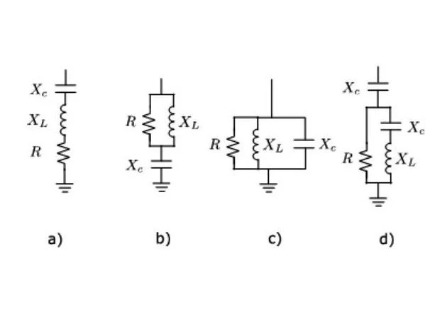
A passive harmonic filter uses capacitors and inductors that are tuned to remove particular harmonic frequencies. See Figure 7. The passive harmonic filter works like a band-pass or low-pass filter in an electronic circuit. It allows low frequencies (60 Hz) to pass through unchanged while removing higher frequencies at 180 Hz and above. Passive harmonic filters can be difficult to use because they often cause other problems like ringing, unwanted resonances, and overcompensation. Single-phase harmonics sources like SMPSs generally do not generate very much phase shift between current and voltage. Therefore, a passive filter can easily cause a circuit to switch from lagging to leading. In addition, passive harmonic filters tend to be fairly large and can be somewhat expensive.
Figure 7. A passive harmonic filter uses a set of resistors, capacitors, and inductors tuned to remove harmonic frequencies. Image courtesy PSCAD
Active Harmonic Filters
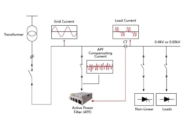
An active harmonic filter uses electronics to provide a variable impedance to remove harmonics from the circuit or to generate an adaptive current waveform that is 180° out of phase with the harmonics.
See Figure 8. Active filters have typically been very expensive and not widely available. However, advances in electronics are making these types of devices more available and cost-effective.
Author: Alex earned a master’s degree in electrical engineering with major emphasis in Power Systems from California State University, Sacramento, USA, with distinction. He is a seasoned Power Systems expert specializing in system protection, wide-area monitoring, and system stability. Currently, he is working as a Senior Electrical Engineer at a leading power transmission company.
Published by Prof. Silviu Darie, PhD (EE), Technical University Cluj Napoca, Romania, Honorary Member of the Romanian Technical Sciences Academy. Email: silviu.darie@enm.utcluj.ro.
Abstract: Based on the author’s experience in designing power systems for critical loads, the paper presents the ways of supplying essential loads, the distribution system layout configuration, the uninterruptible power supply sources (UPS), the UPS modeling and operation, the power system studies by using PTW/SKM professional industrial software.
Key Words: Electrical critical loads, UPS structure and operation, power system modeling procedures, power system studies using professional software.
Abbreviations: UPS – Uninterruptible Power Supply; FDR – Feeder / Cable; CB – Circuit Breaker; FTS – Fast Transfer Switch; PTW/SKM Professional industrial software.
Contributions: A guide for power systems studies with critical loads. Critical loads power system layout; UPS modeling procedures and simulation software settings; power system studies using PTW/SKM professional software.
1. Introduction
The Critical Loads are those to which the power supply has to be maintained under any circumstances and never be interrupted. Such electrical loads are Data Centers, Hospitals, Control Rooms and Control Rooms for Airports, Industrial Control Systems, and oil Shore Platforms. However, there is a need to maintain the power supply to the critical loads during the effective transition to an alternate power supply. The alternate power supply can be the uninterruptible power supply – UPS. The UPS was initially designed for computers. The UPS has a DC battery as an energy storage device. Several UPS are on the market and depend on how they are connected to the critical loads and the UPS configuration [1].
2. System Layout Configuration
Some configurations and structures depend on the size and load profile of the Critical Loads and the application.
One may have the following structure:
• UPS supply from different power sources such as two different Utility Power Supply; • UPS supply from a Utility Power Supply and a Diesel Generator Set.
One presents the typical system layout modeling configuration while industrial software is employed: SKM professional software [1].
Figure 1. Supply from 2 Commercial Sources: Power Utility and Local Generator (SKM Modelling)
Figure 2. Supply from 2 AC Commercial Sources: power system details
3. UPS Description
A UPS is a power supply system with energy storage that ensures the load continues to be supplied even if the primary supply voltage fails (EN 50091-1). The UPSs systems protect against data loss and system damage due to power failures, voltage dips, voltage spikes, under voltage, overvoltage, switching, interference voltages, frequency changes, and harmonic distortion.
A. UPS components: The UPS modules/components shall consist of the following main components:
• Rectifier/charger; • Static inverter; • Fast Transfer Switch (FTS); • Output isolation transformer; • Control panel; • Monitor panel; • Communication panel.
B. The main types of UPS
There are three major types of UPS as follows [Eaton]:
The UPS module shall operate online, fully automatically, in the following modes:
Normal Mode: The inverter shall continuously supply the critical load. The rectifier/charger shall derive power from the commercial AC source and shall supply DC power to the inverter while simultaneously float-charging the battery;
Emergency Mode / Battery Operation: When the commercial AC power is outside a –15/+10% window around nominal voltage, the critical load shall continue to be supplied by the inverter, which shall obtain energy from the batteries without any operator intervention. It’s an automatic operation. There shall be no interruption to the critical load upon failure or restoration of the commercial AC source;
Recharge Mode: Upon restoration of the AC source, the rectifier/charger shall recharge the batteries and simultaneously provide power to the inverter. This shall be an automatic function and shall cause no interruption to the critical load;
Bypass Mode: If the UPS module must be removed from the normal mode for overload, load fault, or internal failures, the Fast Transfer Switch (FTS) shall automatically transfer the critical load to the commercial AC power (usually in less than 0.2 seconds). Return from bypass mode to normal mode of operation shall be automatic. Bypass mode shall be capable of being initiated manually without the operation of the static switch from the front control panel.
Generally, a UPS supply system offers uninterrupted power to the AC load by converting DC into AC. UPS differs from an emergency power supply system or a standby generator, as it can protect devices from power outages by one or more connected batteries. The battery run time is relatively short, typically 5 to 15 minutes, but it is long enough to bring the auxiliary power supply online or protect devices from shutting down.
4. UPS modeling for power systems studies
The UPS unit is modeled as two parts: the primary part is connected to the AC power supply, and it is considered as the power system load. The second part is a power source that supplies the critical loads. While PTW/SKM professional software is employed, two UPS pages shall be developed.
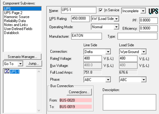
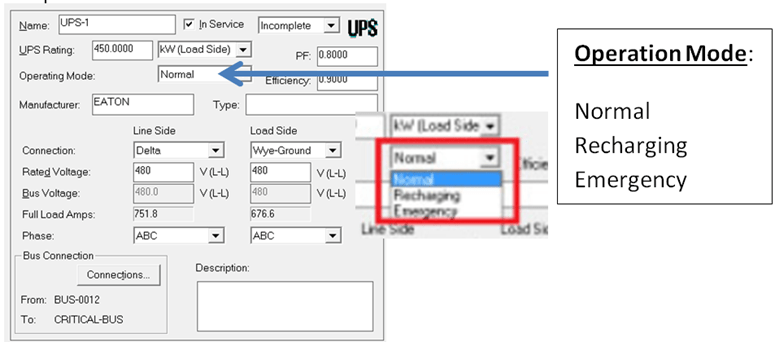
Figure 4.1 The UPS input data is:
• UPS name and manufacturer; • UPS status: in-service or off; • UPS ratings on the load side; • UPS power factor and efficiency; • UPS connection on the line side and load side; • Rated voltages on the line side and load side; • UPS phases.
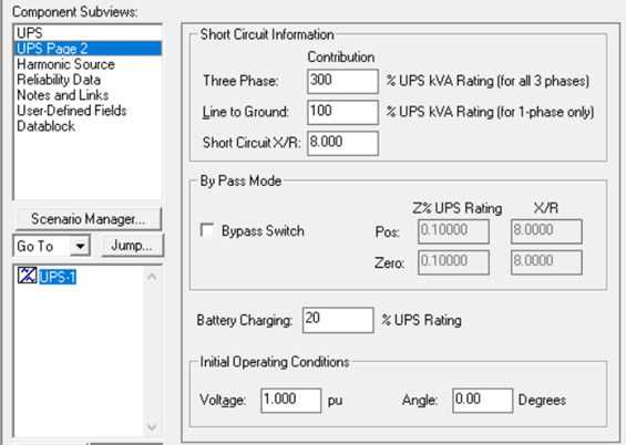
Figure 4.2 The UPS input data shall provide the following:
• UPS short circuit contribution as a percent of the UPS rating; • Short circuit X/R; • Battery charging as a percent of the UPS rating; • Bypass mode provides the technical information for the Fast Transfer Switch (FTS): UPS Zin percent and X/R ratio.
Figure 5.2 UPS Mode of Operation PTW/SKM professional software. Typical, Recharging, Emergency.
Figure 5.3 UPS Recharging Mode of Operation
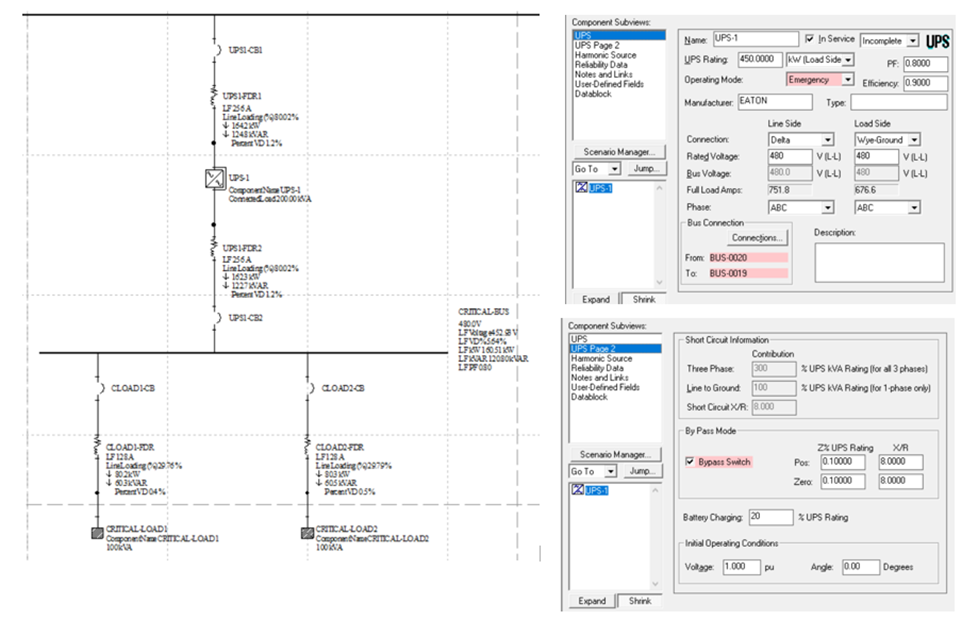
Figure 5.4 UPS Emergency Mode of Operation and Bypass Fast Switch
Note: While UPS is in emergency mode, the FTS is closed in less than 0.2 seconds, consequently protecting the unit.
6. Modeling the Power System with Critical Loads:
The distribution system model shall be developed to be fully integrated and meet the performance specifications requested by the Project Scope of Work.
One recommends that the system model be laid out in multiple drawings/views and in a manner that provides for easy viewing of all analysis results. The one-drawing/view requirement ensures that problem areas found and highlighted by the program are easily seen and not hidden or buried; All one-line symbols shall be adequately spaced to facilitate viewing results on the one-line;
Equipment names used in the modeling software shall be identical to the equipment and naming convention shown on the existing facility drawings and equipment unless conflicts exist; The Consultant Engineer shall discuss facility operation with the designated Facility to determine the possible operating modes of the system and the UPS units. Each system operating mode shall be documented and modeled in the software as “Scenarios” to determine the electrical equipment’s worst-case and associated parameters.
One suggests that the lumped motor groups for MCCs shall be modeled per IEEE standards using groups >50 Hp and <50 Hp. Where motor list data is not available, single lumped groups may be modeled per IEEE-141 “Red Book”;
Medium voltage motors greater than 1.0 kV shall be modeled individually on their respective buses, including all protective phase and ground overcurrent relays and fuses. All substation low voltage power circuit breakers (LVPCB) shall be modeled.
All relay data shall be modeled based on the nameplate data, including manufacturer, type, style, trip device, and settings. Generic substitutions or assumptions shall not be allowed unless data cannot be field verified. All assumptions shall be documented in the report and discussed with the client. All equipment modeling must have a corresponding one-line diagram symbol, meaning there can be no hidden database models. The purpose is for the facility to see all equipment quickly and its associated data, to be able to link documents to the kit as a data repository, etc., and to see problems right on one line. All system modeling shall conform to accept modeling practices as outlined in IEEE-399 “Brown Book.” The Consultant may provide more advanced modeling techniques where compliance with the specification is maintained.
The following guidelines are offered as an aid to determine which technique may be the most appropriate for a particular system operation condition:
7. Power Systems Studies
The power systems simulation generates a TWIN that creates a mirror between a digital model replica and the real world. With all the features integrated into the TWIN, including the requested model date base, one may test power system performance under several conditions.
7.1 Power Flow Analysis
Power Flow / Load Flow is a critical task. The convergence of Power Flow demonstrates that the power system model is feasible and the input data are consistent.
Several methods are employed for Power Flow. The most typical are:
• Seidel Gauss; • Newton Raphson; • Fast Decoupled
Some experimentation is recommended to determine the best methods for each power system model.
The following guidelines are proposed as an aid to determining both the UPS modeling layout and the UPS input data:
• Check the critical loads with the designer; if the distribution system already exists, use the SCADA and get the loads as measured data (system as built);
• Pay attention to the UPS mode of operation: Normal, Recharging, Emergency, or By-Pass;
• The By-Pass mode is during a fault at the critical bus;
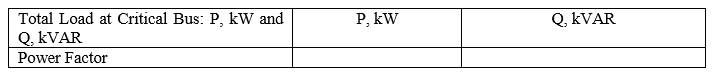
• Pay attention while setting the UPS input data: UPS ratings (P&Q), critical loads P and Q, UPS losses (P&Q); the total load on UPS = critical loads + UPS losses (P&Q) + UPS charging (P&Q);
• UPS input power factor – is not a problem in a modern UPS. The UPS rectifier has reactive and capacitive components, so it will also have a power factor, which must be accounted for when making the upstream electrical connection. The UPS input power factor is a design characteristic usually declared by the manufacturer in the technical specification. With modern IGBT (insulated-gate bipolar transistor) front-end rectifier technology, the input power factor is typically close to unity, 0.99 at 100% nominal load. However, the actual metered input power factor may be slightly different as, for example, highly nonlinear loads can cause the input power factor to decrease slightly. Typically, though, a UPS input power factor will still be in the range of 0.97 – 0.99 and not of great concern. With older technology, using six- or 12-pulse rectifiers, the THDI (total harmonic distortion of current) and power factor require more attention;
• UPS-rated output power factor is a UPS design factor. The rated output power factor describes the maximum active and apparent loading the UPS can tolerate by design. For example, a 100 kVA UPS with a rated output power factor 1.0 can handle loads up to 100 kW active power and 100 kVA apparent power. If the power factor is 0.8, these loads become 80 kW and 100 kV, respectively. The load’s active and prominent power must be known to select and size the UPS correctly. A UPS with a rated power factor of example, 0.8 can handle loads of higher power factor as well – and vice versa;
• A load analysis at the UPS output bus is a good approach for determining the total output load (P&Q) and the UPS power factor [1].
7.2 UPS estimated size
Depending on the possible level of damage in case of a data loss/production stoppage, critical applications require exclusively online UPSs, classification following IEC 62040-3 (double conversion UPS).
One has to calculate the possible damage by conducting a risk analysis with the customer. All other aspects, such as low purchase and operating costs (efficiency), are secondary and must take second place to damage avoidance.
However, the author presents the following simple approach [1]:
a. Get the Critical Input Data from the plant engineer:
.
b. Compute the UPS unit ratings as follows:
.
7.3 Power Flow Analysis Using Industrial Professional Software:
The power system model is generated using the SKM professional software as an exercise. The model is consistent with the requirements of the IEC and IEEE Standards. The model will also be helpful for future power system model upgrades and improve facility operations. The load flow model should be continuously updated as changes are made to the electrical power distribution system. One, in general, recommends that the facility team using this model keep the load flow model updated as changes are made in the system so it is an “as built” model.
PTW/SKM industrial, professional software is employed for system modeling. The PTW/SKM is a powerful industrial power software for designing and analyzing power systems. It is utilized worldwide by consultant engineers, designers, and utility engineers. The PTW/SKM has been on the market for over 38 years. It has a powerful Graphical User Interface (GUI) with several calculations, an extensive power system database, and intuitive display information. The PTW/SKM is used by over 35,000 engineers worldwide, offering specialized Power Tools design and robust modeling and documentation capabilities. Professional training is provided for PTW/SKM users.
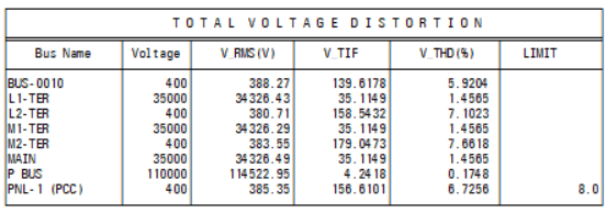
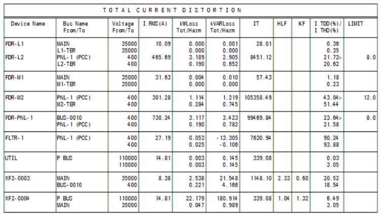
• The load flow shows the bus voltages at all buses and the power flows in all branches: power transformers and lines. The results may be provided as text output results or may be given in the model drawings as Power Flow visualization;
• The convergence of the Power Flow demonstrates that the system is feasible and the system input data is consistent.
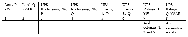
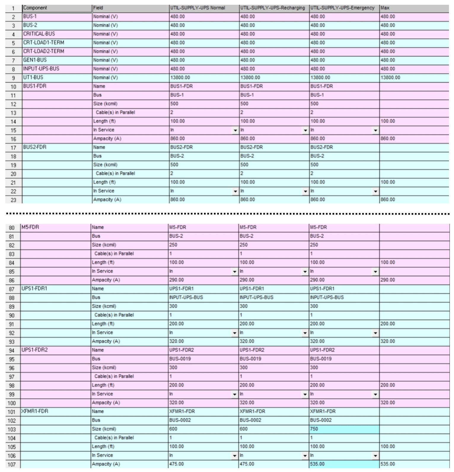
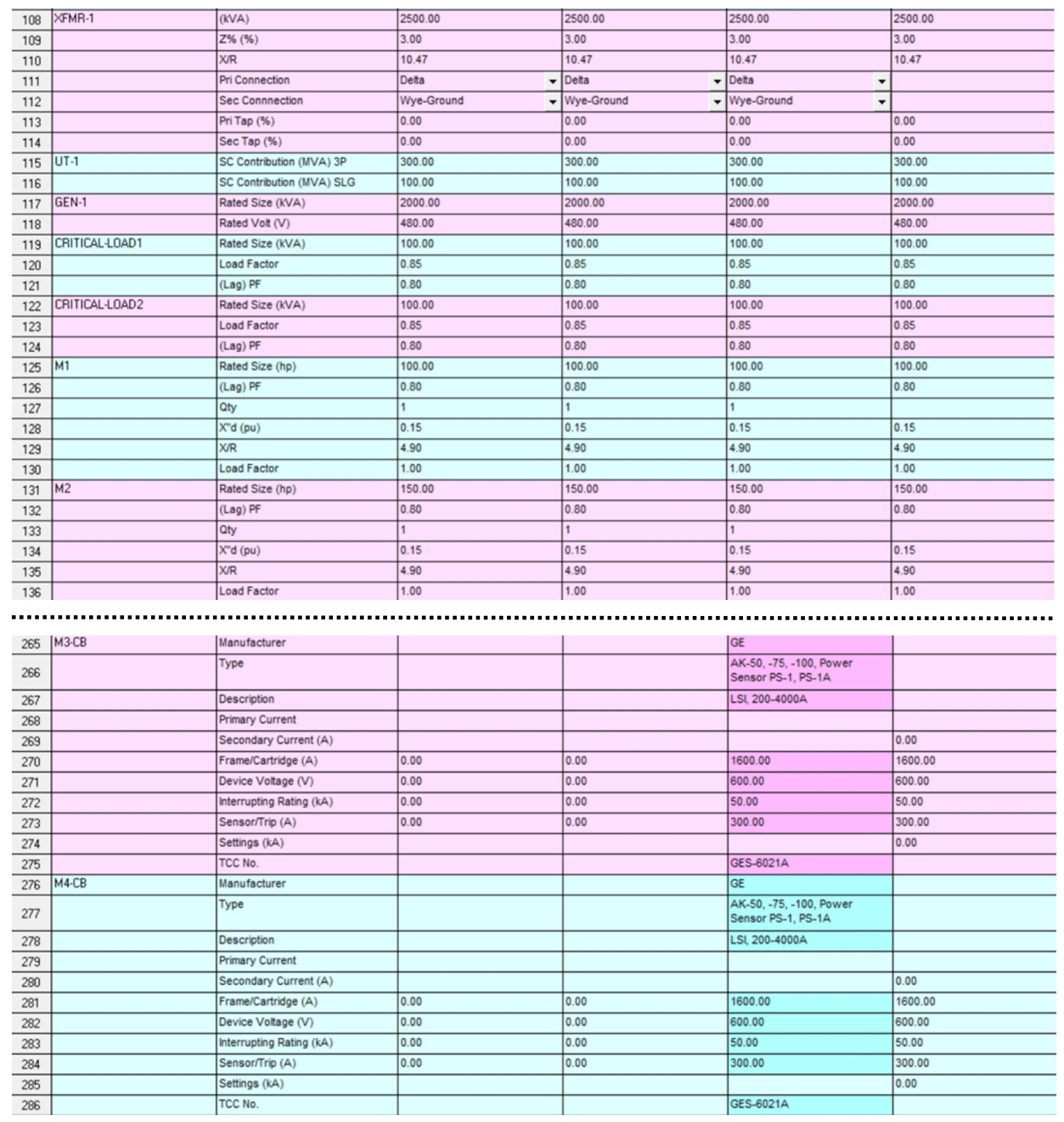
A summary of the model Input Data is shown in Figure 7 below:
Figure 7.1 Model Input Data (overview)
Figure 7.1 Model Input Data (continued)
Figure 7.1 Model Input Data (continued)
Figure 7.1 Model Input Data
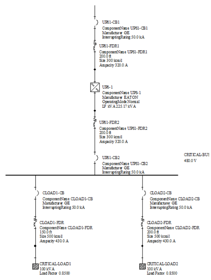
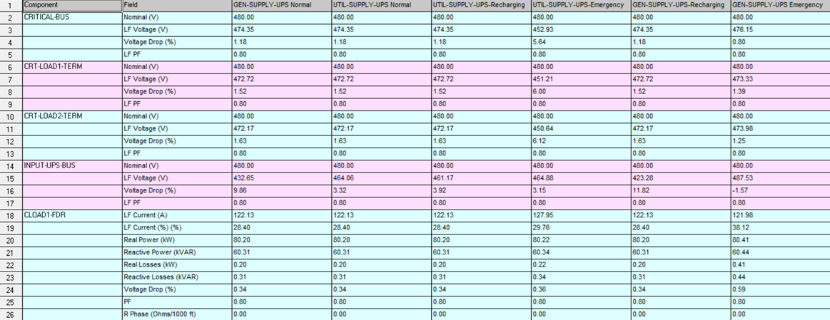
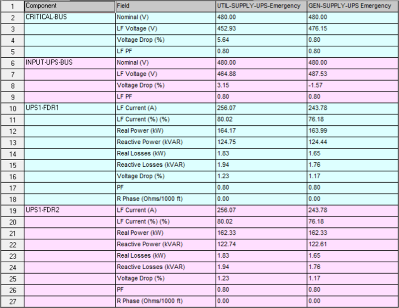
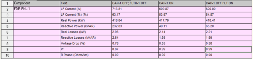
For example, the Power Flow Results for the model shown in Figure 1, the Scenario Utility supply, and the Generator supply for each mode of operation are provided in Figure 7.2 below. The Critical Load is supplied from the UPS unit only briefly. The power flow results are listed on the one-line SKM model.
Figure 7.2 Comparative Power Flow Results
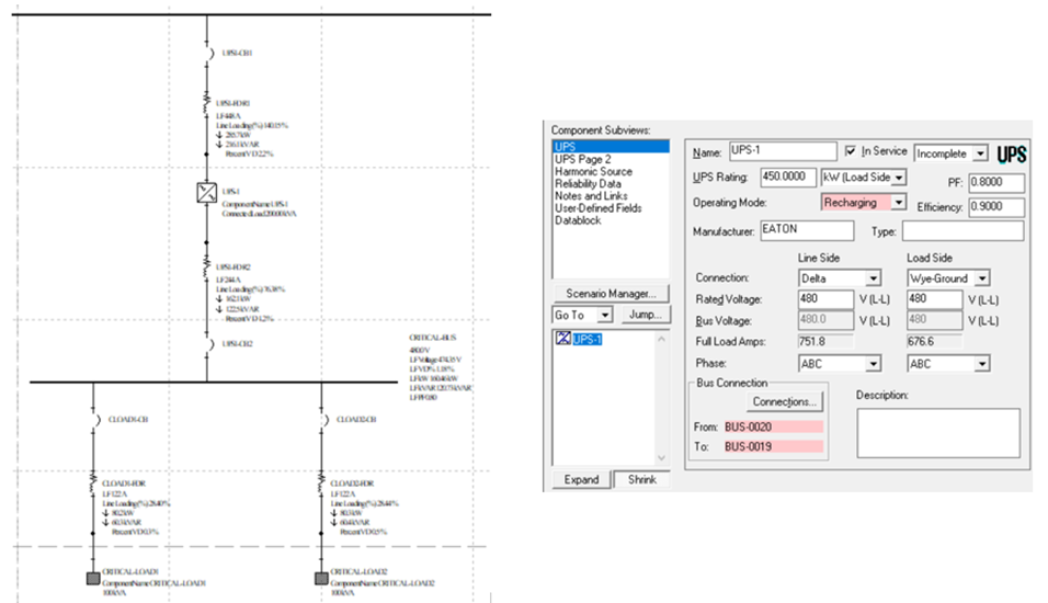
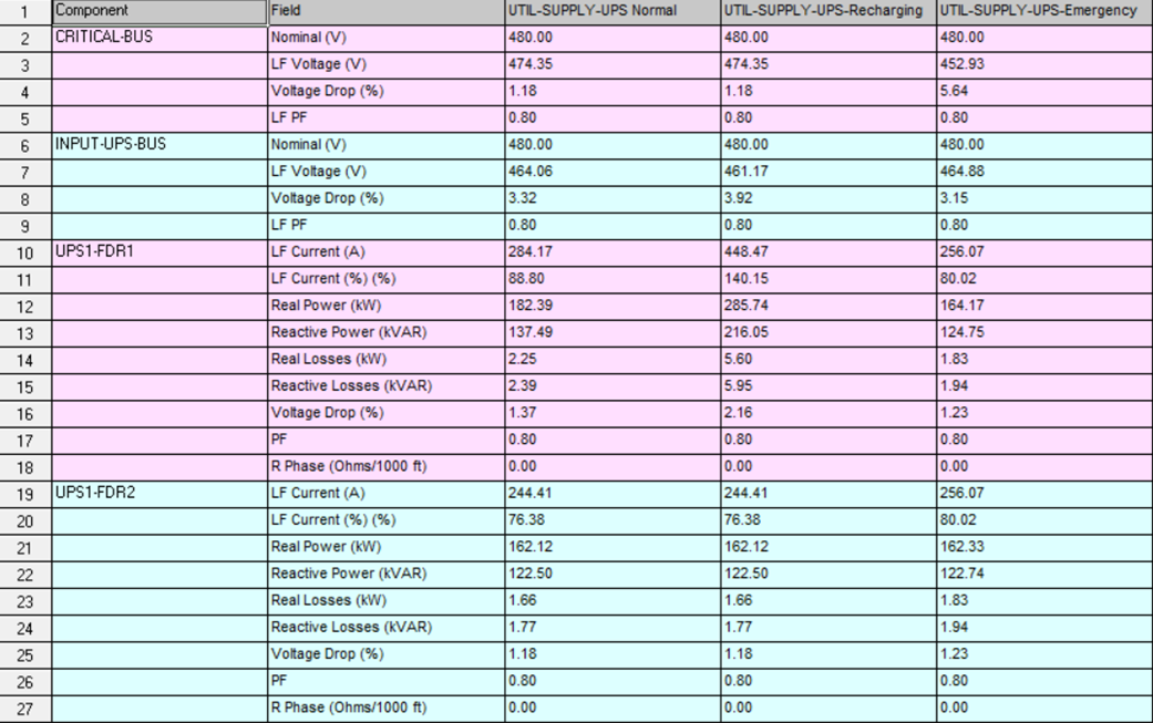
Comparative power flow results, Scenario UTIL-Supply, showing the results for each UPS mode of operation. For this example, during UPS recharging mode, the UPS1-FDR1 is heavily overloaded (140.15%0). Consequently, the size of this feeder would need to be increased.
Figure 7.3 Comparative power flow results, Scenario UTIL-Supply; UPS in recharging mode
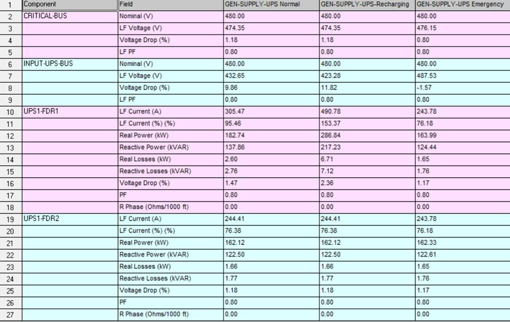
Comparative power flow results, Scenario GEN-Supply, showing the results for each UPS mode of operation. For this example, during UPS recharging mode, the UPS1-FDR1 is heavily overloaded (140.15%0). Consequently, the size of this feeder would need to be increased.
Figure 7.4 Comparative power flow results, Scenario UTIL-Supply; UPS in recharging mode
UPS Overloads and Support Time
For UPSs, the levels and ranges of overloads and support time are [2]:
103% overload 10 minutes to continuous; 125% overload between 30 sec and 10 minutes; 150% overload between 10 sec and 60 sec; 200% overload 10 to 20 cycles (current limit).
Notes: Since the above UPS specifications contain many possible overload and support times, designers must determine if a longer overload time limit provides valuable protection for the critical load [1]. Data Centers with redundant UPS systems features have a significant UPS over-capacity.
The “Power Flow Results” while the UPS unit is in emergency mode are listed below, Figure 7.3. The Fast Transfer Switch (FTS) bypasses the UPS unit, and the current flow on the upper and lower side is the same.
Figure 7.5 Power Flow Results: UPS in Emergency Mode FTS bypasses the UPS Unit
Figure 7.6 Power Flow Results: Supply from Utility or Generator; UPS in Emergency Mode FTS bypasses the UPS Unit
7.4 Short Circuit Analysis:
Short Circuit Analysis is one of the major tasks related to analyzing and planning electric power systems. The scope of a Short Circuit Analysis is as follows:
• Verify the circuit current path against short-circuit current stress (electrical, mechanical, and thermal); • Evaluate and verify the interrupting capacity of existing switching devices; • Calculate and set up adequate system protective device settings; • Evaluate the system-wide post-fault voltage profile during a fault at a particular point; • Improve the system layout design to minimize the effect of system faults.
Short Circuit Current at CRT-LOAD1-TERM (critical LOAD 1 terminal bus) is presented in Figure 7.7: the Scenario Normal; UPS Bypass Operation Mode.
In the bypass mode, the UPS units are protected against the faults. The Fast Transfer Switch (FTS) moves the UPS unit into bypass mode in less than 0.2 seconds. The short branch circuit current is listed in the figure capture listed below, Figure 7:
Figure 7.7 Short Circuit at Bus CRT-LOAD1-TERM
Note: The fast transfer switch (FTS) bypasses the UPS in less than 0.2 seconds and consequently protects the UPS unit. It is represented by the bypass function on page 2 of the SKM UPS editor.
7.5 Protective Device Coordination
Any electrical distribution system has only one purpose: to provide a continuous energy supply to utilize equipment at a reasonable cost. When a fault occurs in a system, it is necessary to clear the spot to provide safety to personnel, protect the circuit elements, and prevent unnecessary power outages. This feature is achieved by using appropriate and proper protections. We apply protective equipment such as lightning arresters, surge capacitors, reactors, and circuit interrupting devices to accomplish this protection function. Any protection project requires two steps
• The selection of the proper device to do the task;
• Select the correct settings for the devices so they will operate selectively with other devices to disconnect that portion of the system in trouble and with as little effect on the rest of the system as possible.
A power system protection project requires not only proper device selection but also wants to achieve the best coordination possible with the equipment we decided to buy. The statement “Coordination and Selectivity” are, in a sense, complementary terms and are used to describe the relative speeds at which two protective devices operate for the same fault current.
A power system protection project requires not only proper device selection but also wants to achieve the best coordination possible with the equipment we decided to buy. The statement “Coordination and Selectivity” are, in a sense, complementary terms and are used to describe the relative speeds at which two protective devices operate for the same fault current.
Coordination Studies:
A coordination study involves selecting and setting all the protective devices from the load upstream to the power supply. In selecting or developing these protective devices, a comparison is made of the operating times of all the devices in response to various levels of overcurrent. The objective, of course, is to design a selectively coordinated electrical power system.
Coordination procedure [1]:
The following procedure should be followed when conducting a coordination study:
• Start the coordination process from the bottom of the circuit and select a convenient voltage base. Usually, the lowest system voltage will be chosen. The Time-current graphical interface is automatically associated with the specified path;
• Specify protection points. These include the motor starting curve with the current and starting times, magnetizing inrush points, and the limits for specific protective paths the user selects. Do not select more than five protective devices for one protective course;
• Using the overlay principle, trace the curves for all protective devices on a composite graph, selecting ratings or settings that will provide overcurrent protection and ensure no overlapping of curves.
Notes [9]:
1. When coordinating IDMTL relays, the interval is usually 0.3-0.4 seconds; The interval consists of the following components: Circuit breaker opening 0.08 seconds (5 cycles). Relay over travel 0.10 seconds. Safety factor for CT saturation, settings errors, etc.: 0.22 seconds;
2. When coordinating relays with downstream fuses, the circuit opening time does not exist for the fuse, and the interval may be reduced accordingly; the time margin between the fuse total clearing curve and the up-stream relay curve could be as low as 0.1 seconds where clearing times below 1 second are involved;
3. When low-voltage circuit breakers equipped with direct-acting trip units are coordinated with relayed circuit breakers, the coordination time interval is usually regarded as 0.3 seconds;
4. When coordinating CBs equipped with direct-acting trip units, the characteristics curves should not overlap.
Generally, only a slight separation is planned between the different characteristic curves. If CBs are in series, the overlaps are accepted.
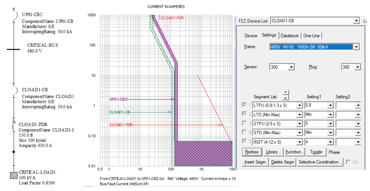
One starts by selecting the protective paths from the bottom part of the power system. A few PDC paths are presented in Figures 7.8, 7.9, and 7.10, while SKM professional software is employed.
UPS must transfer to bypass operation mode to provide enough fault-clearing current to trip the load circuit breaker in a load-side fault.
• Long duration inverter overload capability does not help – inverter does not have sufficient fault current to clear the fault;
• Trying to sustain a fault on the inverter (waiting for the O/L timer) will stress or damage the inverter and result in an output voltage drop;
• If bypass is unavailable – UPS will eventually trip off if the fault isn’t cleared, or the load will fail due to under voltage.
Additional considerations required to determine the robustness and suitability of a UPS system are:
• Maximum continuous temperature rating of UPS running at full load; • Cooling system employed within UPS; • Placement of fans for increased life and elimination of hot spots in the event of fan failure; • Redundancy of fans and fan failure alarms; • Proper handling of fault currents to reduce stress on UPS and loads.
Figure 7.8 PDC Path: From CRITICAL-LOAD1 to UPS-1-CB
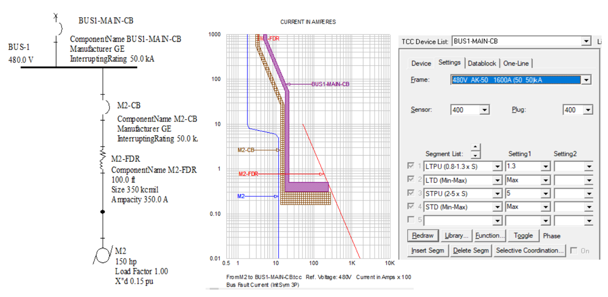
Figure 7.9 PDC Path: Motor M1 to BUS1
Figure 7.10 PDC Path: XFMR-1 Protection
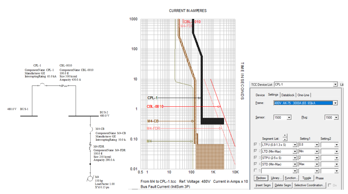
Figure 7.11 PDC Path: From M4 to BUS-1
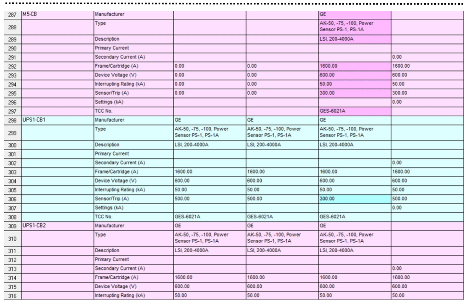
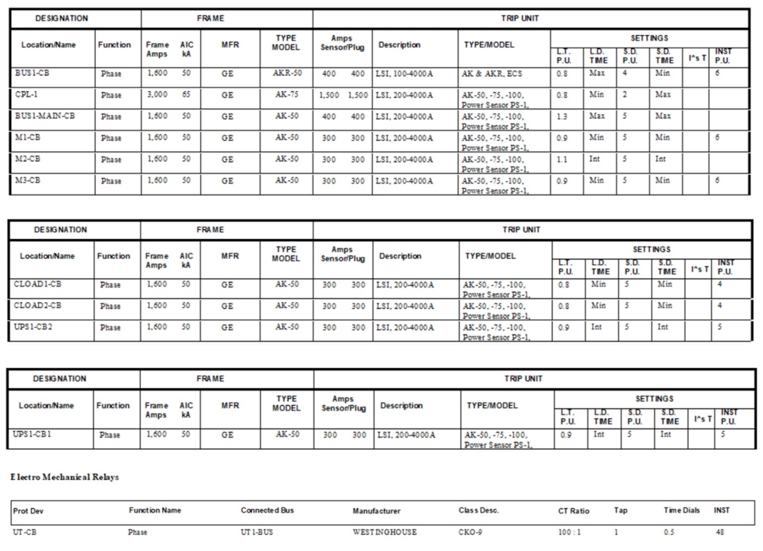
Table 7.1 – LV CBs Types, Frame, and Settings
.
8. Conclusions
The paper presents how to supply the critical electrical loads, the power system layout configuration, uninterruptible power supply (UPS) structure, modeling, and operation. The procedure for the power system studies Power Flow, Short Circuit, and Protective Devices Coordination using industrial, professional software – SKM is documented. Uninterruptible power supply (UPS) systems ensure continuous supply to critical loads and quality power. The UPS system design requires the proper technique, installation, and maintenance.
References
[1] Darie, S.: Modeling UPS for Critical Loads: Training Manuals (2005 to 2015), Power Analytics Corporation, San Diego, USA. [2] SKM Power Software: UPS Units Modeling, 2016. [3] CENELEC – EN 50091-1 Uninterruptible Power Supply. Part 1. General and Safety Requirements. [4] IEC 62040-3 Uninterruptible Power Supply (UPS); Part 3. Method of Specifying the Performance and test requirements. [5] ISO / IEC 9003,2018. Software Engineering Guidelines for applying ISO 9001, 2008 to Computer Software. [6] IEEE Brown Book, IEEE Std. 399, 2015. [7] IEEE Red Book, IEEE Std. 141, 2014. [8] IEEE Std. 142-1991, “Recommended Practice for Grounding of Industrial and Commercial Power Systems” (IEEE Green Book). [9] IEEE Std. 242-1986, “Recommended Practice for Protection and Coordination of Industrial and Commercial Power Systems” (IEEE Buff Book). [10] IEEE Std. 1100-1992, “Recommended Practice for Powering and Grounding Sensitive Electronic Equipment” (IEEE Emerald Book). [11] APS, Schneider Electric: Selection of the UPS Configuration, APS Schneider Electric, 2012. Kevin McCarthy, Victor Avelar: Comparing UPS System Design Configuration. White Paper 75, Revision 3, Schneider Electric, 2016. [12] Piller Power Systems: Isolated-Parallel UPS Configuration. [13] Powerware 9315 (200 to 500 kVA) Static Uninterruptible Power Supply, Guide; Specification Models 225, 250, 300. [14] 400 500 kVA, Power Ware 2003; [15] IEC 62040-1, 2008. TEST REPORT Uninterruptible Power Systems (UPS) – Part 1: General and Safety requirements for UPS.
Author:Prof. Silviu Darie, PhD (EE)
Author: Prof. Silviu Darie, PhD (EE), Technical University Cluj Napoca, Honorary Member of Romanian Technical Sciences Academy, Former VP Power Analytics Corporation, USA.
Prof. Dr. Daries has more than 20 years’ work experience with Power Analytics products, and nearly 40 years of university-level electrical engineering instruction and industry consultancy in power system analysis computer applications, electrical power quality, transmission pricing, embedded generation, computer aided power system analysis and design. In addition to earning both his doctorate and master’s degrees in electrical engineering, he has authored or co-authored hundreds of technical books, student manuals, technical papers, and research projects.
Dr. Darie is a former professor of power systems and electrical engineering in Technical University of Cluj Napoca, Romania, and University of Cape Town, South Africa, as well as a former visiting professor in École polytechnique fédérale de Lausanne, Switzerland. He has received several awards and recognitions throughout his years of expertise including the Award Professor for Life of Faculty of Engineering, University of Cape Town 1993, Romanian National Research Award. Since 2005 he is the Vice President of Consulting and Engineering for Power Analytics Corporation.
Dr. Darie led nearly 180 electrical power projects worldwide; he constructed 18 prototypes designed for mass production, holds three patents, and is experienced in most leading software programs for electrical engineering. He has provided services to clients worldwide, and is a registered professional engineer in Romania, South Africa, and New Zealand.
Contact address: Prof. Silviu Darie, Ph.D., P.E., Romania: Bd. 21 Decembrie 1989, No. 104 Bl. L1, Sc. 1, Ap. 8 Cluj Napoca, 400124 Romania Mobile: +40728312222 Email: silviu.darie@gmail.com, Silviu.darie@enm.utcluj.ro
Published by U.S. Department of Energy – Energy Efficiency and Renewable Energy Alternative Fuels Data Center
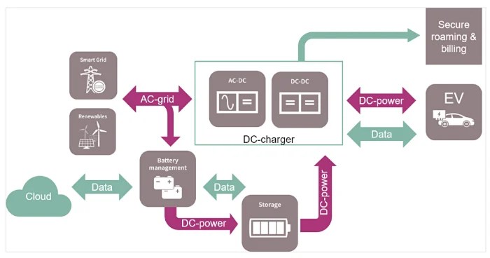
Consumers and fleets considering electric vehicles (EVs)—which include all-electric vehicles and plug-in hybrid electric vehicles (PHEVs)—need access to charging stations. For most drivers, this starts with charging at home or at fleet facilities. Charging stations at workplaces and public destinations may help bolster market acceptance by offering more flexible charging opportunities at commonly visited locations. Community leaders can find out more through PEV readiness planning, including case studies of ongoing successes. The EVI-Pro Lite tool is also available to estimate the quantity and type of charging infrastructure necessary to support regional adoption of EVs by state or city/urban area and to determine how EV charging will impact electricity demand.
Charging the growing number of EVs in use requires a robust network of stations for both consumers and fleets. The Alternative Fueling Station Locator allows users to search for public and private charging stations. Quarterly reports on electric vehicle charging station trends show the growth of public and private charging and assess the current state of charging infrastructure in the United States. Suggest new charging stations for inclusion in the Station Locator using the Submit New Station form. Suggest updates to existing charging stations by selecting “Report a change” on the station details page.
Photo: Charging ports. Image used courtesy of afdc.energy.gov
The SAE J1772 charge port (right) on a vehicle can be used to accept charge with Level 1 or 2 charging equipment. The DC fast charge port (left) uses a different type of connector. In this photo, it is a CHAdeMO.
Charging Infrastructure Terminology
The charging infrastructure industry has aligned with a common standard called the Open Charge Point Interface (OCPI) protocol with this hierarchy for charging stations: location, electric vehicle supply equipment (EVSE) port, and connector. The Alternative Fuels Data Center and the Station Locator use the following charging infrastructure definitions:
• Station Location: A station location is a site with one or more EVSE ports at the same address. Examples include a parking garage or a mall parking lot.
• EVSE Port: An EVSE port provides power to charge only one vehicle at a time even though it may have multiple connectors. The unit that houses EVSE ports is sometimes called a charging post, which can have one or more EVSE ports.
• Connector: A connector is what is plugged into a vehicle to charge it. Multiple connectors and connector types (such as CHAdeMO and CCS) can be available on one EVSE port, but only one vehicle will charge at a time. Connectors are sometimes called plugs.
Charging Infrastructure – 1 Station Location. Image used courtesy of afdc.energy.gov
Charging Equipment
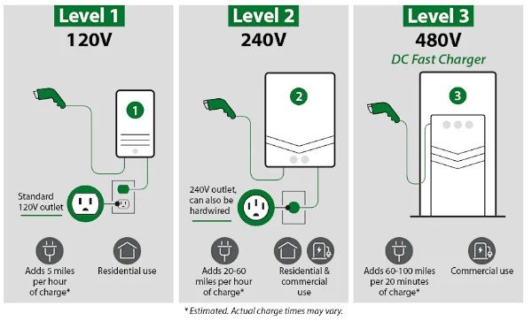
Charging equipment for EVs is classified by the rate at which the batteries are charged. Charging times vary based on how depleted the battery is, how much energy it holds, the type of battery, and the type of charging equipment (e.g., charging level, charger power output, and electrical service specifications). The charging time can range from less than 20 minutes to 20 hours or more, depending on these factors. When choosing equipment for a specific application, many factors, such as networking, payment capabilities, and operation and maintenance, should be considered.
Level 1 Charging
Approximately 5 miles of range per 1 hour of charging*
J1772 connector
Alternating Current (AC) Level 1 equipment (often referred to simply as Level 1) provides charging through a 120 volt (V) AC plug. Most, if not all, EVs will come with a portable Level 1 cordset, so no additional charging equipment is required. On one end of the cord is a standard NEMA connector (for example, a NEMA 5-15, which is a common three-prong household plug), and on the other end is an SAE J1772 standard connector (often referred to simply as J1772, shown in the above image). The J1772 connector plugs into the car’s J1772 charge port, and the NEMA connector plugs into a standard NEMA wall outlet. Note that Tesla vehicles have a unique connector. All Tesla vehicles come with a J1772 adapter, which allows them to use non-Tesla charging equipment.
Level 1 charging is typically used when there is only a 120 V outlet available, such as while charging at home, but can easily provide charging for most of a driver’s needs. For example, 8 hours of charging at 120 V can replenish about 40 miles of electric range for a mid-size EV. As of 2021, less than 2% of public EVSE ports in the United States were Level 1.
* Assumes 1.9 kW charging power
Level 2 Charging
Approximately 25 miles of range per 1 hour of charging†
J1772 connector
Tesla connector
AC Level 2 equipment (often referred to simply as Level 2) offers charging through 240 V (typical in residential applications) or 208 V (typical in commercial applications) electrical service. Most homes have 240 V service available, and because Level 2 equipment can charge a typical EV battery overnight, EV owners commonly install it for home charging. Level 2 equipment is also commonly used for public and workplace charging. This charging option can operate at up to 80 amperes (Amp) and 19.2 kW. However, most residential Level 2 equipment operates at lower power. Many of these units operate at up to 30 Amps, delivering 7.2 kW of power. These units require a dedicated 40-Amp circuit to comply with the National Electric Code requirements in Article 625. As of 2021, over 80% of public EVSE ports in the United States were Level 2.
Level 2 charging equipment uses the same J1772 connector that Level 1 equipment uses. All commercially available EVs in the United States have the ability to charge using Level 1 and Level 2 charging equipment.
Tesla vehicles have a unique connector that works for all their charging options, including their Level 2 Destination Chargers and chargers for home. All Tesla vehicles come with a J1772 adapter, which allows them to use non-Tesla charging equipment.
† Assumes 6.6 kW charging power
DC Fast Charging
Approximately 100 to 200+ miles of range per 30 minutes of charging‡
CCS connector
CHAdeMO connector
Tesla connector
Direct-current (DC) fast charging equipment (typically a three-phase AC input) enables rapid charging along heavy traffic corridors at installed stations. As of 2021, over 15% of public EVSE ports in the United States were DC fast chargers. DC fast charging is projected to increase due to fleets adopting medium- and heavy-duty EVs (e.g., commercial trucks and vans and transit), as well as the installation of fast charging hubs for transportation network companies (e.g., Uber and Lyft) and other applications.
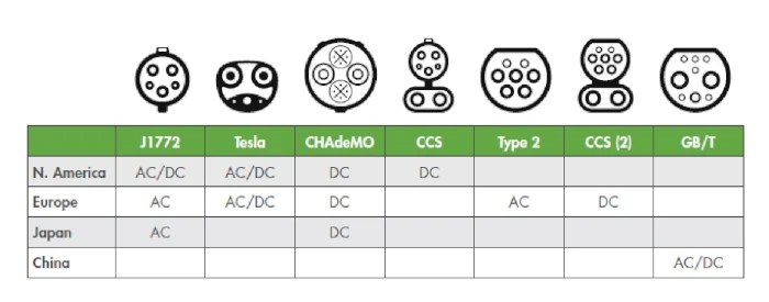
There are three types of DC fast charging systems, depending on the type of charge port on the vehicle: SAE Combined Charging System (CCS), CHAdeMO, and Tesla.
The CCS connector (also known as SAE J1772 combo) is unique because a driver can use the same charge port when charging with AC Level 1, Level 2, or DC fast charging equipment. The only difference is that the DC fast charging connector has two additional bottom pins. Most EV models entering the market today can charge using the CCS connector.
The CHAdeMO connector is another common DC fast connector type.
Tesla vehicles have a unique connector that works for all their charging levels including their fast charging option, called a Supercharger. Although Tesla vehicles do not have a CHAdeMO charge port and do not come with a CHAdeMO adapter, Tesla does sell an adapter.
‡ Charging power varies by vehicle and battery state of charge.
Published by Józef LORENC, Krzysztof ŁOWCZOWSKI, Bogdan STASZAK Politechnika Poznańska, Instytut Elektroenergetyki
Abstract. In this paper possibilities for improvement of earth fault protection by adjustment of protective relay settings due to change of neutral point impedance in medium voltage networks are presented.
Streszczenie. W artykule przedstawiono zagadnienia dotyczące możliwości poprawy skuteczności działania zabezpieczeń ziemnozwarciowych typu YY0 poprzez dostosowanie wartości nastawczych do zmian spowodowanych modyfikacją sposobu pracy punktu neutralnego w sieci średniego napięcia. (Zabezpieczenia ziemnozwarciowe wspierane funkcjami adaptacyjnymi).
Słowa kluczowe: punkt neutralny, zwarcie doziemne, admitancja, elektroenergetyczna automatyka zabezpieczeniowa Keywords: neutral point, earth fault, admittance, earth fault protection systems
Introduction
Admittance relay was developed in Poland in Institute of Electrical Power Engineering of Poznan University of Technology [1, 2, 3, 4, 5, 6]. Principle of operation is explained in [7] and [8]. First relays were implemented in distribution system networks at the end of XX century as an analogue construction. Nowadays admittance criterion is implemented in digital protection relays, which are installed in bays of 110/15 kV or medium voltage substations as an decision-making algorithm. Moreover some distribution system operators install admittance based fault passage indicators [9]. In Poland admittance relays are typically installed in compensated medium voltage networks. Another admittance based criteria for protection relays are in the development stage: i.e. Cumulative Phasor Summing [10 ,11] proposes centralized earth-fault protection based on measurements of zero sequence current and voltage. Despite of admittance criteria for detection of high impedance faults, another criteria are being analyzed i.e. [12] proposes wavelet based criteria. New fault feeder detection methods for a resonant grounding system are also presented in [13, 14, 15, 16].
YY0 relay presented in the paper is improvement of original admittance relay. Principle of YY0 relay operation is based on zero sequence admittance growth – ΔY0 during single phase to ground fault and after reconfiguration of an neutral point impedance. Start-up value is given by formula (1) and (2).
.
Where: SI1, SI3, SI4 – signals measured during earth fault before neutral point impedance reconfiguration, ΔYY0n –admittance growth setting, U0n– zero sequence voltage setting value.
Signals “S” are functions of zero sequence current and zero sequence voltage of lines during phase-to-ground fault. Signals S are described by the following formulas (3), (4), (5) and (6).
.
.
Signal S is connected to the zero sequence voltage input of the relay and is described by formula:
.
Coefficients ku, ki, ky and kn are used to convert zero sequence input signals. Coefficients ku, ki, and kn are dimensionless and describe a transformation ratio of instrument transformers (current and voltage transformers) and input divider, whereas ky represents admittance of additional voltage circuit.
Sensitivity of the relay depends on impedance of neutral point and does not depends on zero sequence impedance of line.
Application of active zero sequence current forcing arrangement (ACF) in compensated networks results in growth of measured admittance ΔY0 observed in faulted line, particularly in growth of conductance component – ΔG0, which is proportional to additional resistance connected in neutral point in parallel to Petersen coil.
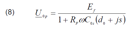
Setting value of YY0 relay is typically in range of 50% of additional resistor conductance. According to operational experience from Poland relays operate effectively up to 2000 Ω of fault resistance. A reason for limited level of detected fault resistance is mostly due to loss of sensitivity of zero sequence voltage component presented in (2) and explained further in (8).
.
where: U0p – zero sequence measured voltage, EF – phase voltage of a network, RF – fault resistance, C0s – earth fault zero sequence capacitance, ω – angular frequency, d0 – damping coefficient of zero sequence impedance described as a ratio of zero sequence conductance and zero sequence susceptance (9), s – detuning coefficient of Petersen coil (10).
.
where: Ld – inductance of Petersen coil.
Analysis of formulas (7) and (8) clearly shows that sensitivity of zero sequence voltage component of YY0 can be improved by changing d0 and s or by decreasing U0n setting value during certain earth fault conditions. However reduction of U0n setting value can only be made during earth fault and after analysis of measured values therefore relay has to be additionally equipped with adaptive algorithm. Two methods of adaptive algorithms are presented in next paragraphs.
Decision making algorithm for shunt impedance connected to neutral point
Fig.1. Characteristic of YY0 protective relay
Based on analysis of formula (7) it is clear that zero sequence voltage level for a given C0sand RF values strongly depends on damping coefficient – d0 and detuning factor – s. During operation of ACF value of d0 coefficient is increased. Alternatively instead of forcing resistor it is possible to connect forcing reactor (reactive zero sequence current forcing arrangement – RCF). In that case value of coefficient of earth fault current compensation detuning s is changed. In practice not only value of detuning factor s can be changed but also its sign.
Another possibility to change s is to disconnect coil, which is normally connected to neutral point of a grounding transformer. If RCF is used an additional criterion which analyses zero sequence susceptance growth of line is required. Therefore universal admittance characteristic presented in the figure 1 should be used. In order to include susceptance region in the characteristic, additional criterion has to be included in decision making algorithm. Criterion is analogical to (1), but signals in I0 current circuit are additionally shifted 90°. As a result characteristic presented in the Figure 1 is created. Area inside a rectangle characteristic (square) is non-operational area. ΔB0 states for susceptance growth necessary for relay operation and ΔG0 is conductance growth necessary for operation.
As is previously described RCF is similar to ACF, however operational experiences shows that in many situations RCF devices can be more effective than ACF. Especially in case of high impedance earth faults.
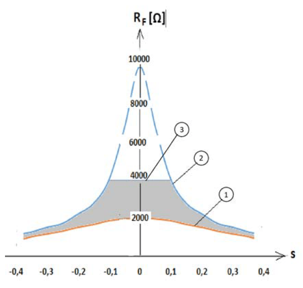
Fig. 2 presents RF = f(s) curves, which describe maximum earth fault resistance seen by YY0 relay in 15 kV compensated network with total ground fault current equals to 120 A. Analysis of curves allows us to conclude that in typical compensated polish networks with detuning factor lower than 0,1 region of detected fault can be significantly bigger if RCF device is used (curve 2) comparing to ACF (curve 1). A phenomena is explained by the fact that negative influence of RCF reactance on zero sequence voltage is lower than in case of ACF.
Fig.2. Maximum fault resistances detected by YY0 relay after operation of active/reactive zero sequence current forcing arrangements
Curves 1 and 2 presents the effectiveness of YY0 relay for earth fault detection after operation of RCF or ACF which enforces 20% rise of a total earth fault current. It is assumed that U0n set value is 15% of phase voltage of a network. Moreover it is assumed that phase-to-ground capacitance is equal in all phases (symmetrical network) and natural damping factor d0 is smaller than 0,04.
In practice effectiveness of YY0 during operation of RCF device is limited by curve 3. Maximal effectiveness (4000 Ω) can be achieved when detuning coefficient after operation of RCF is reduced to 0,1. Following conditions can occur only when:
– network is undercompensated (detuning is no bigger than – 0,1; s = – 0,1) and after operation of RCF network becomes overcompensated (detuning factor is no bigger than 0,1),
– network is overcompensated (detuning factor is no bigger than 0,1; s = 0,1) and after operation of RCF network becomes undercompensated (detuning factor is no bigger than – 0,1; s = – 0,1).
Effectiveness of an earth fault detection is reduced for all other detuning factors. When operation of RCF results in relatively big detuning factor, an effectiveness of earth fault detection will be reduced to 2000 Ω so it will be lower than effectiveness after operation of ACF.
Adaptive algorithm of ACF and RCF compares different variants and choose a better one –ACF or ACF and optimal control of shunt impedance. It is recommended to reduce reactance of coil if network is undercompensated and to increase reactance when network is overcompensated. System for shunt impedance control is presented in the Fig. 3. Control algorithm, which is responsible for measuring voltage level and tuning of Petersen coil plays an important role in the system. RCF increases an earth fault current by connection of additional reactance LNW or reduce a ground fault current (reduce inductive current) by disconnecting a reactance, which is normally connected between neutral point of grounding transformer and a ground. In order to operate properly the system needs to measure detuning factor continuously. Commonly used systems for active compensation and passive systems for control of an earth fault parameters ensure access to necessary parameters.
Fig.3. Control system of shunt, neutral point impedance
Connection of additional resistance to neutral point is justified only when fault resistance is low (relatively big value of U0p – i.e. above 50% of phase voltage) or when detuning factor (absolute) is too big. It is also possible to make a decision about ACF activation based on level of natural asymmetry of a network.
Adaptive settings
As is explained in previous paragraphs an effectiveness of YY0 operation is limited by sensitivity of zero sequence voltage component. In typical polish networks start-up values of voltage are in range of 0,15-0,2 of phase voltage. Specific value is determined by natural phase-to-ground asymmetry of a network and resonance effect during normal operating conditions of a network. As a result of the phenomena voltage is increased permanently during normal operation conditions. Voltage rise is described by formula (11).
.
where: Uasn – voltage resulting from zero-sequence leakage and natural asymmetry, U0rez – voltage resulting from resonance effect between phase-to-ground capacitance of a network and Petersen coil.
One can clearly observe that an amplitude of the voltage could be easily reduced by increasing d0 and s factors. The detuning is however not recommended since an earth fault current extinguishing capabilities of a Petersen fault are reduced. The best condition to extinguish an electric arc can be observed when coefficient of detuning of earth fault current compensation equals 0 – coil current fully compensates a capacitive current of a network. Consequently to reduce negative aspect of resonance effect it is only possible to apply devices, which increase phase-to-ground damping factor. In typical compensated medium voltage networks in Poland and typical ACF systems damping can be raised to approximately 0,2, in these way a voltage resulting from resonance effect is reduced a few times. As a result less restricted requirements could be used during selection of U0n starting values. Reduction of U0nsettings usually improves effectiveness of YY0 relay and increases the range of detected high impedance faults.
Voltage effects resulting from operation of ACF became the foundation for development of conductance protection decision algorithm making in Institute of Electrical Power Engineering of Poznan University of Technology. Adaptive functions are included in this algorithm [8]. Similar functions can be implemented in YY0 relay, which operates according to following rules:
– adaptive function is activated only during resistance fault and when U0p is below Uonafter operation of ACF device,
– setting value is changed only after additional resistive component of a current is detected (effect of ACF operation), – when adaptive function is activated a set value of voltage criterion is reduced and setting of conduction rise is increased,
– reduction of U0p is between 15% to 5% of phase voltage,
– a value of conductance rise depends on ratio of U0p measured before and after operation of PFR and typically is lower than 150% of base value
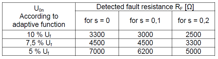
After taking into account defined network parameters a performance analysis of YY0 with adaptive function is performed. Partial results of the analysis are presented in the table 1.
Table 1. Values of fault resistance detected by YY0 relay with adaptive function
.
One can easily notice that thanks to adaptive settings during harsh conditions – high resistance faults (above a few thousands ohms), an effectiveness of earth fault detection is significantly increased. Possibility of reduction U0n setting to 0,05 in well compensated network allows for detection of earth faults with fault resistance above 7000 Ω. In case of networks with a big share of overhead lines and capacitive current in range of 80 – 90 A the effectiveness can be even higher – up to 10000 Ω.
REFERENCES
[1] Lorenc J., Marszałkiewicz K., Andruszkiewicz J., Admittance Criteria for Earth Fault Detection in Substation Automation Systems in Polish Distribution Power Networks. CIRED, Birmingham (1997), Publication IEEE, No. 438 (1997) [2] Florkowski W., Lorenc J., Maćkowiak M., Musierowicz K., Sposób i układ wybiorczego zabezpieczenia od jednofazowych zwarć z ziemią w sieci o małym prądzie ziemnozwarciowym, Patent PL Nr 116699 [3] Lorenc J., Rakowska A., Staszak B., Limitation of Earth-Fault Disturbances and their Effects in Medium Voltage Overhead Lines. Przegląd Elektrotechniczny, no. 4 (2007), ss. 75-79 [4] Lorenc J., Torbus M., Staszak B., Automatyczna sterowanie kompensacją ziemnozwarciową w sieciach SN przy wykorzystaniu miernika parametrów ziemnozwarciowych, Wiadomości Elektrotechniczne, no. 12 (2013) [5] Lorenc J., Musierowicz K., Sposób i układ do pomiaru stopnia skompensowania prądu ziemnozwarciowego w sieciach kompensowanych średniego napięcia, Patent PL Nr 150320 [6] Lorenc J., Staszak B., Wiśniewski A., Sposób i układ do wykrywania zwarć wysokooporowych w liniach pracujących w kompensowanej sieci średniego napięcia, Patent PL Nr 226282. [7] Lorenc J., Admitancyjne zabezpieczenia ziemnozwarciowe. Wydawnictwo Politechniki Poznańskiej,j (2007) [8] Wahlroos A., Altonen J., Compensated networks and admittance based earth fault protection, ABB library, (2011) [9] Altonen J., Wahlroos A., Performance of Modern Fault Passage Indicator Concept in Compensated MV-Networks, CIRED Workshop – Helsinki, (2016) [10] Wahlroos A., Altonen J., Application of Novel Multi-frequency Neutral Admittance Method into Earth-Fault Protection in Compensated MV-networks, 12th IET International Conference on Developments in Power System Protection, (2014) [11] Balcerek P., Fulczyk M., Rosołowski E., Iżykowski J., Pierz P., New algorithm for determination of faulty feeder in distribution network, 11th IET International Conference on Developments in Power Systems Protection, (2012) [12] Michalik M., Rebizant W., Łukowicz M., Lee S.-J. Kang S.H., Wavelet Transform Approach to High Impedance Fault Detection in MV Networks, IEEE Russia Power Tech, (2005) [13] Mou-Fa Guo, Nien-Che Yang, Features-clustering-based earth fault detection using singular-value decomposition and fuzzy c-means in resonant grounding distribution systems, Electrical Power and Energy Systems 93 (2017), ss. 97–108 [14] Xiangning Lin, Shuohao Ke, Yan Gao, Bing Wang, Pei Liu, A selective single-phase-to-ground fault protection for neutral uneffectively grounded systems, Electrical Power and Energy Systems, 33 (2011), ss. 1012–1017 [15] Wahlroos A., Altonen J., Pekkala H-M., Post-fault oscillation phenomenon in compensated MV-networks challenges earth-fault protection, 23rd International Conference on Electricity Distribution, Lyon, (2015) [16] Linčiks J., Baranovskis D., Single Phase Earth Fault Location in the Medium Voltage Distribution Networks, Scientific proceedings of Riga Technical University, The 50th International Scientific Conference Power and electrical engineering, (2009)
Authors: prof. dr hab. inż. Józef Lorenc, Politechnika Poznańska, Instytut Elektroenergetyki, ul. Piotrowo 3a, 60-965 Poznań, E-mail: jozef.lorenc@put.poznan.pl; mgr inż. Krzysztof Łowczowski, Politechnika Poznańska, Instytut Elektroenergetyki, ul. Piotrowo 3a, 60-965 Poznań, E-mail: krzysztof.lowczowski@put.poznan.pl; dr inż. Bogdan Staszak, Politechnika Poznańska, Instytut Elektroenergetyki, ul. Piotrowo 3a, 60-965 Poznań, E-mail: bogdan.staszak @put.poznan.pl;
Source & Publisher Item Identifier: PRZEGLĄD ELEKTROTECHNICZNY, ISSN 0033-2097, R. 94 NR 8/2018. doi:10.15199/48.2018.08.31
Published by Ryan Hsu, Bright Toward Industrial Co., Ltd., EE Power – Industry Article: Insulation Failure Detection in EV Batteries, May 15, 2023.
One of the issues with electric vehicle batteries is insulation failure. A proven approach to detecting and correcting this failure lies in ground-fault detection. However, as higher voltages become increasingly common in electric vehicle battery systems, finding the right MOSFET to handle these voltages is vital.
One of the issues with electric vehicle (EV) batteries is insulation failure, and the ability to detect and correct it is critical. A proven approach lies in ground-fault detection, requiring solid-state MOSFET relays. However, as higher voltages become increasingly common in EV battery systems, finding the right type of MOSFET to handle these voltages reliably is vital.
As electric vehicles become more powerful and require more voltage, MOSFET relays with higher operating voltages are necessary. Image used courtesy of Pixabay
Insulation Failure in EV Batteries
When insulation materials lose their insulation ability, it can cause resistance to decrease, leading to hazards for the battery management system (BMS) that can lead to shorter battery life or a risk of fire.
Therefore, in the design and use of a BMS, it is essential to be aware of these factors that can cause insulation breakdown and take appropriate measures to prevent it. Such factors include:
•Overload: Applying too much voltage to insulation materials can cause a breakdown.
•Contamination: Dust, moisture, or other pollutants can weaken insulation materials, causing breakdown.
•Aging: Over time, insulation materials may break down due to thermal, chemical, or mechanical degradation.
•Physical damage: Scratches, cuts, or other physical damage to insulation materials can create a current path, causing breakdown.
•Voltage stress: Over time, the application of AC electric fields can cause insulation materials to break down.
•Temperature: High temperatures may make insulation materials brittle and prone to breakdown.
Early EVs had issues with slow charging times and short ranges, which led to engineers increasing the total voltage and current rating to improve these characteristics. However, because of higher currents and voltages, there was the potential for shorter battery life and overheating to the point of fire. Engineers began developing insulation monitoring functions for EV BMSes to address this issue.
Preventing Insulation Failure
The most common method for preventing insulation failure is measuring the resistance of the dielectric by detecting the ground-fault current.
When the insulation of a battery cell fails, the energized conductor will come into contact with metal that is not intended to carry current. That metal is usually bonded to part of the equipment-grounding conductor and becomes a path of least resistance to electrical currents, constituting a ground fault. The presence of a ground fault can be used to activate an alarm signal using a MOSFET relay between the current sensors and the ground. This insulation monitor/detection function in BMS ensures that the battery insulation is healthy and no leakage occurs. The insulation detection system aims to identify and isolate faults, ensuring the safety and reliability of the battery system and protecting the batteries from premature failure.
In the ground fault detection approach, the MOSFET is switching high voltage from the BMS through a non-contact relay and a set of series/parallel resistors, as shown in Figure 1. The MCU (microcontroller unit) then measures the voltage drop to calculate the insulation resistance of the BMS. The insulation resistance value must comply with safety regulations: AC 500 ohms/V and DC 100 ohms/V; if it is too low, an alarm signal is activated to provide immediate protection against potential hazards.
Figure 1. A typical circuit for ground fault detection. Image used courtesy of Bright Toward
Furthermore, it is necessary to promptly check and repair equipment or systems to restore them to normal operation. Maintenance checks can also be performed on the insulation detection system to ensure its proper functioning and provide accurate data.
However, when selecting the MOS relay, it must withstand a higher voltage than the battery pack’s nominal voltage. For example, a battery pack with an 800 V nominal voltage typically requires a relay with a load voltage greater than 1600 V.
SiC MOSFETs Versus Si MOSFETs
SiC (silicon carbide) MOSFETs provide some definitive benefits compared to the Silicon-based equivalents. SiC-based Opto-MOSFET relays, in particular, offer greater load voltages, excellent switching speeds, and more energy-efficient performance. And while they are used in a range of applications such as industrial robotics, security, and telecommunications, they have been extremely useful for insulation failure detection in electric vehicles–especially those involving higher voltages.
Why Opto-SiC MOSFET Relays are a Better Solution
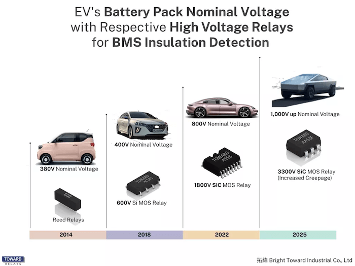
The relay used in BMS insulation detection has changed over the years, as illustrated in Figure 2, beginning with reed relays when the nominal voltage was 380 V. As the nominal voltage for battery systems increased, the operating voltage for the relays also increased. That increase required MOSFETs to switch to much higher voltage levels.
Note that when the nominal voltage was 400 V, Si MOS Relays were sufficient. However, a different semiconductor material was needed to handle greater voltages efficiently.
Figure 2. How BMS insulation detection system relays have evolved through the years. Image used courtesy of Bright Toward
A Si-based Opto-MOSFET relay’s physical limit is around 1500 V, which is not high enough for newer, higher-voltage battery systems that demand 1800 V operating voltages. Hence, the move to SiC MOSFETs.
Opto-SiC MOSFET Relays
Bright Toward’s Opto-SiC MOSFET relays for automotive applications are ideal for EV insulation failure detection, including some rated for 3300 V. The two main series are the 58 Series and the 53 Series.
58 Series is rated for a peak load voltage of 1800 V, with the 53 Series rated at 3300 V. Also, note that 6600 V Opto-SiC MOSFET Relays will be released soon. The AA58 series is AEC-Q101 certified and rated for a peak load voltage of 1800 V. They are used not only for EV BMS but also for energy storage systems and automatic test equipment — and represent the most innovative and highest voltage MOS relay in the market.
The AS58F series has similar ratings and applications as the AA58 series but also includes creepage clearances of ≥ 8 mm for input-output and ≥ 8 mm between drain pins of MOSFETs for safety certification requirements. Major automotive companies have already validated the 1800 V Opto-SiC MOSFET Relays (AA58, AS58) with ongoing mass production.
As the demand for higher load voltage solid state relays increases, Bright Toward has developed SiC-based Opto-MOSFET Relays to improve and increase load voltage for applications, including EV battery insulation fault detection and BMS battery balancing and other applications in industries as diverse as telecommunications and aviation.
Author: Ryan Hsu, is the Marketing Manager at Bright Toward Industrial Co., Ltd, a company based in Taiwan with over 30 years of experience in manufacturing reed relays and solid state relays for various industries, with a strong focus on BMS and IC testing. The company’s dedication to providing innovative and reliable solutions in these industries has been a key driver of their success. The company’s annual revenue of 55 million USD is a testament to its extensive experience and expertise in these industries.
Published by G. A. Mendonça1, H. A. Pereira1,2 and S. R. Silva1, 1 Graduate Program in Electrical Engineering – Universidade Federal de Minas Gerais Av. Antônio Carlos 6627, 31270-901, Belo Horizonte, MG, Brazil. Phone: +55-31-3409-4842, e-mail: gforti@gmail.com, heverton.pereira@ufv.com.br, selenios@dee.ufmg.br 2 Department of Electrical Engineering, Universidade Federal de Viçosa Av. P.H.Rolfs S/N,36570-000, Viçosa, MG, Brazil
Abstract. Wind power plants are playing an important role in renewable energy generation in this decade. With the enhancements in its technology, mainly based on the aggregation of power electronics, many studies have been carried for evaluating their impact in power quality. Although the Brazilian Electrical System National Operator, who is responsible for transmission and generation system management, has suggested a procedure for such studies, there are many aspects related to the simulation algorithm and the electrical components modelling that are left aside from the problem, without an adequate reasoning of its impacts on power quality simulation results.
This paper presents a detailed analysis of a wind farm impact on the Brazilian distribution system power quality. Both internal (wind park elements) and external (power grid) components modelling effects on harmonic propagation are considered, and these effects are evaluated
Keywords: Wind Farm, Harmonic Analysis, Frequency Domain Simulation, Power System Modelling, Simulation Software;
1. Introduction
Adequate modelling of electrical components has always been a concern when analysing harmonic penetration. Several works had been carried out in order to investigate the problems incurred from evaluating harmonic studies with a comprehensive analysis of the used approach.
Many of these studies, [1]-[4], discuss the methods which can be used to evaluate harmonic distortion: single and three phase system representation, time and frequency domain, etc. These works have lead to what is considered to be the most important aspect in harmonic studies, a sense of how these methods can affect the quality of the results. But it does not state the difference in improvement from one to another in a quantity matter.
Another important subject when dealing with harmonic propagation is the electrical components modelling. The difficulty in finding the proper equivalent to represent the system’s main equipment without letting the problem become neither too complex, impracticable to simulate, nor too simple, with inaccurate results.
Using a wind power plant as the study case, a sensibility analysis can evaluate the impact of the assumptions that one can make in this sort of study. For that, two computer simulation programs will be used. The Alternate Transient Program – ATP, which has several available equipments models for applications ranging from steady state to very complex transient analysis, will be used for comparing component equivalents with different complexity degree. On the other hand, DIgSILENT PowerFactory, an engineering tool specifically designed for Power System Analysis, will be used to compare the effects of systems degrees of representation.
2. System Description
The studied wind is similar to one of the 54 wind parks connected to the Brazilian grid. It consists of a collector substation and three feeders with a total of 28 wind generators. The wind farm system, which operates with a voltage of 34.5 kV, is connected to the grid through a step-up transformer, 34.5/69 kV, and a transmission line with 21 km. Then, a substation elevates the voltage to 230 kV in order to connect wind farm with the primary transmission system.
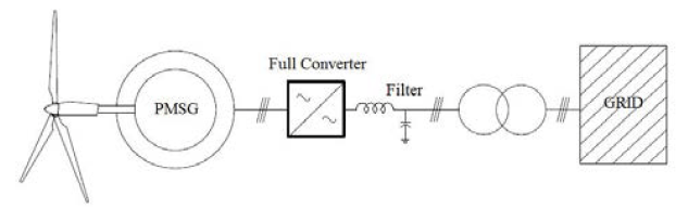
In that wind farm, the wind turbine generators – WTG are connected in three parallel groups, one composed of ten and two of nine units. Figure 1 illustrates the first group with ten wind generators. The other two groups are constructed analogously. Each wind generator consists of a permanent magnet synchronous generator – PMSG, with a full converter, each unit been capable of generating up to 1.5 MVA. In order to meet power quality requirements, the converter is followed by a second-order low-pass filter that helps smoothing the voltage waveform. This LC filter is composed of a series 0.15mH inductor and a shunt 500μF capacitor per phase. A scheme illustrating the PMSG is pictured in Figure 2.
Fig.1. One-line diagram for Group I WTG of the simulated wind park
Fig.2. Wind turbine with PMSG, back-to-back PWM converter and output filter
Although the wind generator technology affects substantially the harmonic analysis, this paper will consider one technology, modelled as harmonic current source. It will help concentrate in how the system modelling affects the overall result, considering only one technology and its harmonic current spectrum, listed in Table I.
The electrical components parameters of the simulated wind park were obtained from commercial wind farms, manufacturer engineering catalogue and electrical standards. Electrical cable and transformer’s characteristics are presented in Tables II and III, respectively.
3. Electrical Equipment Modelling
For the modelling of the electrical system, the following assumptions are considered:
1) All electrical supplies are balanced 2) The system components are symmetrical 3) All wind turbines are equal
Having considered that, the wind turbines were modelled as harmonic current sources without specifying the harmonic phase angle spectrum. As recommended by [5], the lack of diversity presented in most wind parks could be interpreted as a high probability of the harmonics to be in phase. Also, since all electrical components are symmetrical, the system will be treated as single-phase one.
Table I. – WTG Harmonic Spectrum
.
Table II. – Conductor Electrical Parameters
.
Table III. – Transformer Specification and Parameters
.
Focusing in the degree of system representation and the equipment modelling, the next sections will discuss them in detail.
A. Cable Modelling
The distribution system of the wind farm is composed by single-core XLPE cables with the conductor size ranging from 70 mm2 to 185 mm2. The parameters were obtained from manufacture catalogues and used to feed the models.
The electrical parameters listed in these catalogues, which are usually gathered from measured data, were evaluated against a simulated model. In [6], the author discusses the modelling of these cables in EMTP-type programs, e.g. ATP, delineating a procedure which helps to overcome all inaccuracies that the model might present. This procedure was concerned mainly with transient analysis. Thus, it concentrates on providing common materials properties, on representing semiconductor screens properly, on analysing the significance of grounding condition of sheath, etc. Therefore, the electrical parameters calculated according with this procedure can be used to assess the accuracy of catalogue data.
A XLPE single-core 300 mm2 cable was modelled according with [6], at ATP’s Line/Cable Constant – LCC routine, and the distributed line component. The maximum error found for both amplitude and phase angle was 4.02% and 1.47%, respectively.
Therefore, the LCC model present in ATP gives a better response for transient phenomena, but for limited frequency range simulations, such as harmonic analysis, the simpler distributed parameter model is sufficient.
B. Transformer Modelling
Usually, in steady-state studies, e.g. short-circuit and load flow, transformers are modelled simply by a series impedance. Considerations relating winding stray capacitance are generally made for higher frequency studies, where some authors state that its effects are only noticeable for frequencies higher than 4 kHz [1].
This assumption can be validated using ATP. The program has several transformer models available, but the most complete one is the hybrid transformer, which represents stray capacitance. Typical values for this parameter can be found in [7].
For the analysis up to 3 kHz, a simple voltage divider circuit simulation showed that the maximum difference between the results with and without the capacitance effect was 1.67% for the amplitude and 3.86% for the phase angle.
C. Distribution and Transmission System Modelling
What degree of representation should be considered as accurately sufficient? This question always bothered when investigating broader frequency spectrum problems. If representing the entire network is impractical, estimating its behaviour from point of common coupling – PCC, short-circuit impedance, as used sometimes, is unrealistic [4].
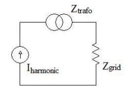
In [4], the author suggests a system equivalent which is based on the prominence of low order resonances. It represents the system impedance with an L-C-L equivalent circuit, estimated from short-circuit impedance and the first two resonant frequencies, i.e. parallel and series.
The Electric System National Operator (ONS in Portuguese) is the entity responsible for coordinating and controlling the operation of generation and transmission facilities in the National Interconnected Power System. It offers information on Brazilian’s system, including electrical parameters of transmission line, transformer, capacitor bank, etc. It also provides the system data base built in the programs developed by CEPEL. The data base can be converted for harmonic analysis program, HarmZs, to find the frequency response at any bus compounding the Brazilian grid.
For this study, a few considerations were made in order to simplify the analysis. All transmission lines are modelled as a single equivalent nominal π-model, all machines impedances were neglected and all loads were modelled as parallel loads. The frequency response observed in the PCC is pictured in Figure 3, which also shows the frequency response obtained from the short-circuit parameters and with the L-C-L equivalent circuit calculated according to [4]
Fig.3. System frequency response at the PCC
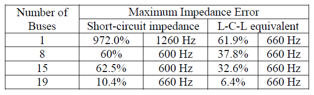
With the system data collected from the ONS database, the primary transmission was modelled in PowerFactory with eight, fifteen and nineteen buses. In each case, the frequency response was obtained with two types of representations of the part of system not explicitly modelled: short-circuit impedance and L-C-L circuit equivalent at each boundary bus. Table IV illustrates the maximum absolute error observed for the resonance amplitude and frequency in each approach when compared with the entire system response.
Table IV. – System representation error
.
The prior analysis also considered secondary distribution system, representing lower voltage equipment. Thus, for a sensibility assessment, a second simulation was carried out. Starting with the representation which incurred the best result, with nineteen EHV buses, the system was simulated without any equipment rated lower than 230 kV. Then, the system complexity was slightly increased by representing the components connected to the point of common coupling. The comparison of these two results is summarized in Table V.
Table V. – System representation error
.
As the high voltage transmission system has lower losses, its impedance dominates the frequency response. But, it’s not necessary to model accurately the entire primary transmission network. The reduced system frequency response converged to the expected result with nineteen buses. As for the secondary distribution system, the model should represent at least those equipments which are connected to the PCC.
D. Full Converter PMSG Turbine Modelling
For the present harmonic propagation study, the wind turbines are modelled as harmonic current source in parallel with a fundamental frequency source [8]. The synchronous machine parameters were set in order to give the fundamental power, 1.5 MW, without affecting the impedance frequency spectrum. Figure 6 illustrates the model used in PowerFactory.
The harmonic current listed on Table I was collected through measurements made according to IEC 61400-21. Since it is concerned the WTG power quality impact, all quantities were collected after the converter filter, before the transformer’s low voltage side. Thus, the harmonic spectrum obtained from turbine manufactures already considers the filter effect, but not its influence over the system’s impedance. Neglecting this effect could under or overestimate some dangerous resonant frequencies.
Therefore, the harmonic current spectre will be recalculated according to equation (1). The harmonic current injection, modelled as illustrated in Figure 4, will be modified according to Figure 5. Zgrid is the short circuit impedance at the 34.5 kV bus.
.
Fig.4. WTG model
Fig.5. WTG model
Fig.6. WTG model
Fig.7. Modified WTG model
The filter gain is illustrated in Figure 8. For this study, two values of short-circuit power were used: 150 MVA and 1500 MVA. The first value used is the short-circuit impedance at the 34.5kV bus for the study case system. The second value was used to find the impact of this parameter in the overall result, estimating the situation during IEC testing to obtain the current spectrum.
From (1), it can be seen that the filter inductor has no effect on the output current. The modified WTG model that will be simulated in PowerFactory is illustrated Figure 7.
E. Aggregate Model for Large Wind Power Plants
Finding an aggregated model for wind power plant to simplify the analysis has become a powerful tool when investigating large wind farms. IEC [5] proposes an aggregation method based on the assumption that the wind turbines and their converters are unequal. However, most wind farms turbines have equal technologies.
Fig.8. Calculated filter gain
Fig.9. Harmonic current spectrum
The limits that this method implies are very well discussed in [9], where the author proposes a method of aggregation using two-port network theorem, the equivalent ABCD parameters are obtained from individual cable parameter, which also modify the harmonic current injection. The wind park is composed with n cable sections, as illustrated Figure 10, and does not considers the generator transformer. The wind turbine current emissions are reflected to the high-voltage side of the transformer.
Fig.10. Wind turbine group for aggregation method
A second circuit simplification is discussed in [10], where the derivation is based on apparent power losses. In this approach the author scales the transformer impedance by the number of units. The results obtained from both methods are discussed in the next section, where the wind farm system is studied.
4. Study Case
The Wind Power System studied in the present paper is partially illustrated in Figure 1. First, it was simulated so that the two aggregation methods discussed previously could be evaluated.
As stated in [9], the first method is based on two-port network theory where the medium-voltage network is modelled by its linear passive elements. The harmonic current injection is considered on the high side of the WTG. Therefore, generator transformers are not considered. For the second method, all transformers were scaled according with the number of parallel units.
The impedance frequency response seen from the 34.5 kV bus was compared for the three cases: the system with 10 WTG and the aggregated equivalent using both methods. The maximum error found in each case was 8.32% and 21.74%, respectively. Secondly, the total harmonic distortions – THD, observed in the 34.5 kV and the 69 kV buses are listed in Table VI.
Considering both methods with and without the filter explicitly modelled, the results were compared through the 34.5 kV and the 69 kV bus THD values. Table VI gives the results.
The harmonic current injection was modified and the filter’s capacitor was explicitly modelling in each case, except for the first method of aggregation, which only uses the current seen from the high-voltage side of the transformers. The THD results for this simulation are also presented in Table VI.
Table VI. – Total Harmonic Distortion
.
Despite of having a better result when comparing the impedance frequency response, the voltage distortion obtained from the first aggregation method did not meet with the expected.
The study case was also simulated focusing on the impact that the distribution system modelling has on the harmonic results. The wind farm was simulated with its internal system aggregated by the second method, which showed better results.
The first two cases simulated the wind farm with the transmission system seen from the PCC represented with the short-circuit impedance and the L-C-L circuit equivalent. The last two results were obtained based on a more detailed system modelling, where 19 buses from the EHV system was explicitly represented. This simulation permitted the analysis of the transmission line impedance effect, where it can be evaluated using the distributed parameter or the concentrated parameter model. The results obtained for these cases are summarized in Table VIII.
The harmonic current was recalculated according with (1) considering two different cases: Zgrid obtained from a short-circuit power of 150 MVA and 1500 MVA. The different current spectrums, illustrated in Figure 9, were simulated to compare the effect of this parameter on the result.
Table VII. – Transmission system modelled as an equivalent
.
Considering the last case, with the transmission system represented with 19 EHV busses and the transmission lines modelled with distributed parameters, as a more accurate result, it can be seen that assumptions made for the equipment modelling play an important role in harmonic penetration analysis.
Simulating the system without accounting with the WTG second-order low pass filter presented very severe results. Also, from the point of view of the grid, the difference in the filter gain by altering the short-circuit power, Zgrid in (1), showed very little difference from each other. When comparing the first two results, the limitations of simpler representation are evident. Considering the THD at the 230 kV bus, when the system is modelled as a short-circuit impedance, the error presented is 53.4%. With the L-C-L equivalent, the error for was as high as 37.6%. The transmission line modelling affected very little the harmonic distortion results. The highest error observed for the THD at the 230 kV bus was 12%.
5. Conclusions
There are several ways to model an electrical system when analysing harmonic propagation. Although several studies propose a rule of thumb when dealing with electrical equipment representation, it always lacks a quantitative comparison against each possibility.
This paper simulates a wind power system with parameters estimated from commercial systems and analysed it, examining the overall impact of system modelling and the degree of representation.
For harmonic studies, cable and transformers models presented in power system analysis engineering software, e.g. DIgSILENT PowerFactory, are very accurate. The degree of representation of external system is important, representing it with the short-circuit impedance at the PCC is very poor. For the presented study case, the result converged for the expected result with the system modelled with 19 busses and considering only secondary distribution system connected to the PCC. Further studies must be carried out in order to verify the accuracy of the reduced representation in other parts of the Brazilian grid. The harmonic source modelling must be analysed beyond the current spectrum measured. Filters used to mitigate the harmonic propagation have an important effect on the system impedance, altering the study results. Another study using time-domain simulation could enhance the analysis of the filter impact.
References
[1] S.J. Ranade and W. Xu, “An Overview of Harmonic Modelling and Simulation”, Tutorial Harmonics Modeling and Simulation, IEEE Power Engineering Society, 1998. [2] J. Arrillaga and N.R. Watson, Power System Harmonics, John Willey and Sons, London (2003), pp. 261-348. [3] CIGRE JTF 36.05.02/14.03.03, “AC System Modelling for AC Filter Design – An Overview of Impedance Modelling”, ELECTRA No. 164, 1996. [4] P.F. Ribeiro, “Guidelines on Distribution System and Load Representation for Harmonic Studies”, in ICHPS V, pp. 272-280, Atlanta, 1992. [5] IEC 61400-21-2008, “Wind Turbine Generator Systems—Part 21: Measurement and Assessment of Power Quality Characteristics of Grid Connected Wind Turbines”. [6] B. Gustavsen, J. Martinez, and D. Durbak, “Parameter Determination for Modeling System Transients – part II: Insulated Cables”, in IEEE Transactions on Power Delivery, vol. 20, no. 3, pp. 2045–2050, 2005. [7] IEEE Std C37.011-2005, “IEEE Application Guide for Transient Recovery Voltage for AC High-Voltage Circuit Breakers Rated on a Symmetrical Current Bases”, pp. 49-53. [8] J. Li, N. Samaan, S. Willians, “Modeling of Large Wind Farms Systems for Dynamic and Harmonic Analysis”, in Transmission and Distribution Conference and Exposition, pp. 1-7, 2008. [9] F. Ghassemi and K. Kah-Leong, “Equivalent Network for Wind Farm Harmonic Assessments”, in IEEE Transactions on Power Delivery, vol. 25, no. 3, pp. 1808-1815, 2010. [10] E. Muljadi, et al, “Equivalencing the Collector System of a Large Wind Power Plant”, in IEEE Power Engineering Society General Meeting, 2006.
Source: European Association for the Development of Renewable Energies, Environment and Power Quality (EA4EPQ). International Conference on Renewable Energies and Power Quality (ICREPQ’12) Santiago de Compostela (Spain), 28th to 30th March, 2012
Published by Joanna KOZIEŁ, Lublin University of Technology, Institute of Electrical Engineering and Electrotechnologies
Abstract. The paper presents the classification of superconducting fault current limiters. In particular the principle of construction and operations of superconducting current limiter of transformer type is presented. Functional physical model of such a limiter, designed, manufactured in the Laboratory of Superconducting Technologies of Institute of Electrical Engineering. The paper presents the results of experimental research and the analysis of the impact of the secondary winding limiter on the performance of superconducting current limiters of a transformer type and the conclusions from the analysis are introduced.
Streszczenie. W artykule zawarto klasyfikację nadprzewodnikowych ograniczników prądu zwarcia. W szczególności przedstawiono zasadę budowy i działania nadprzewodnikowego ogranicznika prądu typu transformatorowego. Omówiono funkcjonalny model fizyczny takiego ogranicznika zaprojektowany wykonany w Pracowni Technologii Nadprzewodnikowych Instytutu Elektrotechniki. Przedstawiono wyniki badań eksperymentalnych, analizę wpływu uzwojenia wtórnego ogranicznika na parametry nadprzewodnikowych ograniczników prądu typu transformatorowego i przedstawiono wynikające z analizy wnioski. (Analiza wpływu impedancji uzwojenia wtórnego na parametry nadprzewodnikowych ograniczników prądu typu transformatorowego).
Słowa kluczowe: nadprzewodnictwo, ograniczenie prądu zwarcia, nadprzewodnikowy ogranicznik prądu typu transformatorowego, impedancja uzwojenia wtórnego. Keywords: superconductivity, limiting of short circuit current, transformer type superconducting fault current limiter, the impact of secondary winding impedance.
Introduction
Superconducting fault current limiters – SFCL are composed of superconducting elements of alternating impedance, being connected in series in an electrical circuit [1], [2]. They show a low impedance while operating in rated conditions of a protected electrical circuit, and high impedance in short circuit conditions in a protected circuit [3].
Fig.1. The state in the superconductivity – the idea of phenomena [4], [5].
The rapid return of capabilities to limit the current after the disappearance of short circuit and long life together with low operating costs are the main advantages of superconducting fault current limiters.
The SFCL superconducting elements work in both the superconducting and in the resistive state. The requirements for SFCL superconducting materials are different than in the case of other superconducting devices intended to operate only in the superconducting state (Fig. 1) [1],[6].
The classification of superconducting fault current
limiters Literature distinguishes between the following superconducting fault current limiter types:
• resistive limiter, • inductive limiter [2],[7-10], • a) systems with an open magnetic core [11], b) systems with a closed magnetic core, • transformer type [12],[13].
You can accept the idea that the transformer type superconducting fault current limiter is a variation of the inductive type superconducting fault current limiter with a magnetic core. The transformer type superconducting fault current limiters have many advantages over resistance and inductive ones because they do not require current culverts, as it is the case of resistance limiters, and do not require secondary superconducting winding either, as it is the case of inductive limiters. In the transformer type superconducting fault current limiters the secondary winding impedance value of a limiter will increase the short circuit impedance during the short circuit, consequently the short circuit current will be limited to the value resulting from the parameters of the superconducting element used. The degree of reduction of the current in the transformer type superconducting fault current limiters is sufficient to limit the short circuit current with very large values.
The principle of the construction and operation of transformer type superconducting fault current limiter
Fig. 2 shows the idea of the construction and operation of transformer type superconducting fault current limiter. The limiter in question is composed of a conventional transformer with copper winding and of a superconducting element R2, shorting the secondary winding of a conventional transformer. The superconducting element is usually an inductor or a bifilar coil, wound with the HTS superconducting tape. The primary copper transformer winding is connected in series with the protected circuit of power grid and the secondary winding is shorted with the HTS superconducting coil, with the critical current value equal to the admissible value of the current of the protected circuit. When the current in the secondary winding of the conventional transformer exceeds, as a result of a short circuit, the value of the critical current of the superconducting winding, the winding loses superconductivity and transits into the resistive state. The HTS coil transition to a resistive state occurs rapidly. Within a few microseconds, the resistance of the secondary side of the transformer and the transformer type superconducting current limiter “changes” in the reactor limiting the current in the protected circuit. With such an activity of the limiter, the short circuit/fault current does not achieve its primary maximum, which protects electrical equipment, especially transformers, from the effects of mechanical forces that can damage the device mechanically.
Fig.2. The construction and operation of transformer type superconducting fault current limiter [4], [14]:
I1 – current of the primary side of the transformer, I2 – current of the secondary side of the transformer, U1 – voltage of the primary side of the transformer, U2 – voltage of the secondary side of the transformer, L1 – self-inductance of the primary side, L2 – self-inductance of the secondary side, US – mains voltage, M – mutual inductance of windings, ZL– load, R2– resistance of the superconducting limiting element.
If the value of the current of the power transmission line I1, which is equal to the current value of the primary side of the serial transformer, is small then the current limiter has a very low impedance (in the superconducting state), because RHTS = 0.
During the short circuit, as a result of the increase in the value of the I1 current the limiter has a high impedance (a resistive state), because the resistance of the superconducting element is significantly higher than zero RHTS> 0 [15].
Fig.3. The model of the cupper transformer Cu with a capacity of 10 kVA [16]
Design and construction of transformer type superconducting fault current limiter model
In the Laboratory of Superconducting Technologies of Institute of Electrical Engineering a functional model of a single-phase transformer type superconducting fault current limiter model was designed and constructed [16].
The limiter consists of a conventional 10 kVA transformer with copper secondary winding shorted with a superconducting element (Fig.3). Table 1 shows the Cu conventional transformer model parameters.
Table 1. Parameters for a transformer model with conventional Cu windings [16].
.
The superconducting element is a superconducting coil composed of two independent windings w1, w2 wound on a common bobbin. This structure allows the configuration of the superconducting element to operate with different values of resistance and inductance of windings: winding w1or w2 windings connected in series or in parallel – either compatibly or contrarily.
Fig.4. The branched characteristics of tapes in the second generation [17]
This allows you to determine the effect of the parameters of the superconducting element on the process of limiting the current by a limiter. Superconducting windings are cooled in a bath of liquid nitrogen. The parameters of the superconducting windings are given in Table 2.
Table 2. Parameters for superconducting coils composed of two independent windings w1and w2made of HTS 2G SCS4050 [16]
.
Both windings are made of HTS 2G SCS4050 superconducting tape produced by SuperPower. This is a tape with a width of 4 mm and a thickness of 0.055 mm [16],[18-20] laminated on both sides with copper, with a critical current Ic = 150 A. Maximum rated current of the superconducting windings is equal to the effective value of the critical current of the superconductor amounting to 82 A.
Fig.5. Windings made of superconducting tapes 2G HTS SCS 4050 [16].
Laboratory research for transformer type superconducting fault current limiter model
Experimental research was conducted in order to verify the possibility to limit the short circuit current by the transformer type current limiter and to determine the level of the current limit with respect to the parameters of the superconducting element (HTS windings configuration) [12]. The research was conducted in Laboratory of Superconducting Technologies in the measurement system shown in Fig. 6.
Fig.6. Short circuit measurement system for transformer type superconducting fault current limiter [16]
The superconducting fault current limiter model is powered by a voltage regulator connected to the power network in separate transformer. The shunts used to perform the current measurement have a value of 1 mV/1 A. The measurements were performed with the use of a measuring PC DAQ Card and LabView software. The short circuit was initiated by the short circuit system. The time of short circuit is 0.05 s.
The analysis was performed for the following superconducting winding configurations w1and w2:
Configuration I – the secondary winding of the Cu transformer shorted with w1 coil, Configuration II – the secondary winding of the Cu transformer shorted with w2 coil; Configuration III – the secondary winding of the Cu transformer shorted with w1 and w2 coils connected in parallel.
The electrical parameters of windings for each configuration of HTS coils are shown in Table 3.
Table 3. The parameters of superconducting windings for the three configurations of windings w1 and w2 [16].
.
Fig. 7 shows the current waveforms on the primary and secondary side of the limiter for the selected configuration of the windings. After the current in the secondary winding of the Cu transformer has crossed the critical current value of the superconducting winding, the surge current (the first impulse of the short circuit current) is limited to the value resulting from the value of the short circuit impedance of the limiter – ZZW (ISC).
Fig.7. The waveforms of primary and secondary currents for II configuration of the superconducting winding [16].
The comparison of the primary current waveforms obtained for all the HTS configurations of the windings shown in Figure 8 compares the number of times the limited surge current exceeds the value of the critical current of the superconducting winding.
Fig.8. The comparison of the primary current waveforms for the three configurations of HTS windings [16].
The short circuit impedance of the limiter Zzw (ISC), is the sum of Cu transformer impedance – ZzwCu (ISCCu) and superconducting winding impedance ZHTS. If we assume for simplicity that ZzwCu (ISCCu) has a constant value, then the impedance value Zzw (ISC) depends on the reactance value XHTS and the resistance RHTS of the HTS winding, thus on the configuration of the winding and on the resistance of the superconducting tape used at the temperature of 77 K. The higher the RHTS and XHTS value, thus the value of the superconducting winding impedance the greater the limitation of the short circuit current. The time after which the limited surge current reaches the expected value of the short circuit current set, for configuration II of the HTS winding, amounts to about 6 ms.
Conclusions
The analyses conducted and experimental research results show that it is possible to build a transformer type superconducting fault current limiter, using the existing conventional transformer with the secondary winding shorted by the superconducting winding made of HTS tape.
The level of limiting the short circuit current, especially the first impulse of the surge current, depends on the value of the short-circuit impedance of the limiter, being the sum of the Cu transformer impedance and HTS winding impedance. HTS winding impedance depends on the winding configuration (inductors or bifilar coils, or many coils connected in series or in parallel), and also on the resistance of the superconducting tape. Selecting the proper HTS tape as well as the appropriate configuration of the superconducting winding, on the assumption of the constant value of the Cu transformer impedance, it is possible to build a transformer type superconducting fault current limiter with a desired level of limiting the short circuit current.
Acknowledgments. I sincerely thank my the promoter prof. Tadeusz Janowski you for any help, patience, kindness during the implementation of my doctoral thesis and my colleagues from the Laboratory of Superconducting Technologies of Institute of Electrical Engineering.
Autor: dr inż. Joanna Kozieł, Lublin University of Technology, Electrical Engineering and Computer Science Faculty, Institute of Electrical Engineering and Electrotechnologies, Lublin ul. Nadbystrzycka 38A, 20-618 Lublin, E-mail: j.koziel@pollub.pl
Source & Publisher Item Identifier: PRZEGLĄD ELEKTROTECHNICZNY, ISSN 0033-2097, R. 92 NR 12/2016. doi:10.15199/48.2016.12.20
Published by Mike Falter, EE Power – Market Insights: Making Sense of Electric Vehicle Charging Options, September 07, 2022.
When it comes to charging your electric vehicle there are several options to consider based on speed, convenience and cost.
In the recent article on the Wallbox acquisition of COIL, EE Power briefly reviewed the Wallbox portfolio of EV charging solutions. EV charging solutions are not all the same and within just the Wallbox portfolio there are multiple solutions with varying charge rates, price points and installation requirements. Charging platforms can be suited to long or short-distance driving, public or home use and can have vastly different installation and operational costs.
In this article, EE Power takes a closer look at the different types of EV charging stations, their capabilities and use cases.
EV Charging Defined by Standards
To start, EV charging infrastructure is largely defined by two main standards. The J1772 SAE standard covers the general physical, electrical, functional and performance requirements to facilitate conductive charging of EVs in North America while IEC 62196 governs similar standards in Europe.
Fast DC charging solution. Image used courtesy of Wallbox
EV Charging Levels
EV charging can be categorized into three different Levels with different power outputs and charge rates:
Level 1 Charging – In North America and Japan Level 1 uses single phase 120 V AC, accessible from a standard residential 3 prong wall socket, to charge the EV through an EVSE (Electric Vehicle Service Equipment) cable and Type 1 J1722 plug that connects to the EV charge port. Level 1 chargers can deliver up to 20 A (2-3 kW @ 120 V) of charge power. This translates to about 5 miles of vehicle range per hour of charge time for a typical EV with 2.5 miles of range per kWh of battery capacity. At these slower rates, Level 1 systems are best used for overnight home charging or shorter-range driving. Note, there is no Level 1 charging in Europe since the standard residential voltage level is 240 V.
Level 2 Charging – These chargers use 240 V AC and are commonly used in public space applications like parking lots, although they can be used in home applications with the proper electrical infrastructure. The Wallbox Pulsar Plus is an example of a Level 2 charging solution. These chargers can be hardwired or connected through a properly rated NEMA plug to a 240 V wall socket. In North America, charge rates with Level 2 systems generally get to about 9.6 kW (40 A @ 240 V single phase) which translates to about 20-25 miles per hour of charge or 4-5 times the rate of Level 1 systems. In Europe, the Middle East and Africa Level 2 chargers use 3 phase AC that can deliver even more power, up to 22 kW (32 A, 3 phase) for residential applications.
Level 3 Charging – Also known as Fast DC charging, this is the fastest way to charge an EV with charge rates well above 100kW. Supernova from Wallbox is a fast-charging solution rated to 130kW that can add up to 120 miles of range to a typical EV in 15 minutes. The Hypernova model (planned for release in 2023) will be a fast charger capable of delivering 350 kW. At 350 kW the GMC Hummer EV pick up with 213 kWh battery capacity can be fully charged in just over 30 minutes. Level 3 achieves these high-power levels by charging at over 480 V DC.
EV Charging Levels. Image used courtesy of Central Hudson
Connecting to the EV Charge Port, Variations by Region
The plug, or connector, is what connects the charge station to the EV, allowing it to deliver power to the high voltage (400 V or more) lithium-ion battery powertrain. The Type 1 J1772 is the standard plug used in single-phase AC Level 1 and Level 2 charging applications in North America and Japan, and supports charge rates up to 10 kW. In Europe, IEC 62196 Type 2 plugs are used for 3 phase AC Level 2 charging applications up to 22 kW.
For DC fast charging the CHAdeMO plug configuration accommodates up to 100 kW and is most common in Japanese models. The CSS (Combined Charging System), or Combo plug, is a clever modification to the J1772 Type 1 plug in North America, or the IEC Type 2 plug in Europe, that adds two extra power contacts to the standard AC connector to support the higher DC charge rates. Due to its versatility, the CSS plug is quickly emerging as the standard for vehicles in North America and Europe. Telsa uses a proprietary plug for its network of fast charging stations but offers adaptors for use with public stations that use either CHAdeMO or CSS.
EV Charging Plug Type by region. Image used courtesy of Blink Charging
The EV charging port will often be configured to accept both AC and DC charging connectors and may have multiple ports. CSS sockets can support both Level 1/Level 2 AC and CSS “Combo” fast DC plugs.
EV charge socket configurations. Image used courtesy of the Driven
EV Onboard Charging Module and DC Fast Charging
Most EVs have an AC/DC converter on board that converts external AC power (Level 1 and 2 charging) to DC for charging the battery powertrain. However, in the case of fast DC charging, utility power is converted to DC externally, so the EVs internal AC/DC converter is bypassed allowing the batteries to be charged directly. In this manner, much higher rates can be achieved since the onboard AC/DC conversion typically limits rates in Level 1 and Level 2 applications.
DC chargers require a lot of power from the grid which can make the costs of operation and installation a lot higher compared with Level 1 or 2 systems. But the benefit is significantly faster charging times and a solution better suited to long range use cases like the US Interstate Highway System. $5 billion in funding was recently allocated through the federal Bipartisan Infrastructure Law to help expand the network of fast charging stations across the Interstate Highway System.
EV onboard charging module for AC and Fast DC stations. Image used courtesy of Springer
Architecture of a DC Fast Charging Station
At its heart, a DC fast charger is a power inverter that converts three phase utility power to the DC current needed to replenish the EV battery powertrain. Typically, line AC power is converted to DC through a controlled rectification stage using an IGBT bridge or similar circuitry. This can be followed by a suitable transformer isolated DC-DC conversion stage that conditions DC power specific to the needs of EV fast charging. Finally, the fast charger communicates with the onboard Battery Management System to properly monitor and regulate the flow of DC power to the EV battery pack.
Fast DC charger architecture. Image used courtesy of Infineon
Author: Mike Falter is Principal and Founder at TechLaunch Strategies.
Published by Prof. Silviu Darie, PhD (EE), Technical University Cluj Napoca, Romania, Honorary Member of the Romanian Technical Sciences Academy. Email: silviu.darie@enm.utcluj.ro.
Abstract: Based on the author’s experience one describes in field tested methodologies which can be employed in solving the frequency-based power quality problems. A generic approach is presented and an experience-based assessment is provided. After defining the main harmonics indices a case study with three (3) scenarios/cases with personal computer application is presented. PTW/SKM professional software is employed.
Keywords: Nonlinear loads, bus voltage total harmonic distortion, (THD-V), branch current total harmonic distortion, (THD-I), total harmonic demand distortion, (TDD), computer aided harmonic analysis, case study computer assisted.
1. Introduction
This paper provides the procedures that one should employ while Harmonics Analysis Investigation is of concern. One should highlight that Harmonic Analysis comprises several steps. The first step is to determine if harmonics exist in the given power systems. Usually this is given by a site survey and site measurements. Please notice that a close cooperation with the plant engineer is a “must-use” dialog. Once that the power system one line is provided and the filed data has been collected building the electrical model follows. Several professional power engineering software can be employed, such as PTW/SKM, ETAP, DigSILENT, CYME, EasyPower, Paladin DesignBase, etc. While the power system is built, all the power system components and system layout should in detail be considered. Once the model is completed, the harmonic sources are generated and then injected at the existing points of harmonics sources. The power system model has to be consistent with the requirements of IEEE 519-2014, IEEE-399 (Brown Book) and IEC 500 standards. As a rule, once the power system is built in any professional power software, always run Power Flow. The convergence of Power Flow demonstrates that the system is feasible and the input data is consistent.
1.1 Methodology
Based on the site survey the study power system layout, power system components data and system operation scenarios are collected. In general, the Harmonics Analysis study is conducted to determine:
• Bus voltage waveform, bus voltage spectrum and bus voltage total distortion THD-V % at Point of Common Coupling (PCC) or at all of the power system panels in the system model, if the project owner requires; Branch current waveform, branch current spectrum and branch current total Distortion THD-I % at all of the branches which fed the panels in the system model;
• One recommends computing the total “Harmonic Voltage” and current indices; this gives the bus voltage fundamental magnitude V1 and the bus actual voltage Vrms considering harmonic contribution; branch current fundamental I1 and branch actual Irms current considering the harmonic contribution;
• The harmonic voltage and current.
1.2 Assumptions
When necessary, assumptions are made based on mutual agreement and with suitable technical and/or the other relevant applicable arguments. Bus IDs, branch names and equipment characteristics are shown on the Computer Program model drawing and project database. Equipment Names should be input as per “project as built”. However, in completing the plant model one uses plant one-line drawings and data from site survey of the existing equipment.
2. Harmonics investigation
2.1 Harmonics indicators
There are several indexes which can be used to measure the harmonics impacts to the power network. The most commonly used indexes are, [3, 6, 8, 9, 11]:
• Total harmonic distortion; • Total harmonic distortion for bus voltage, V-THD (%); • Total harmonic distortion for current, I-THD (%); • Total harmonic demand distortion, TDD for branches; • Telephone interference factors, if this is requested IT.
2.2 Harmonics voltage distortion
Harmonic voltage distortion index Vn% is the r.m.s. amplitude of a harmonic voltage of order “n” expressed as a percentage of the r.m.s. amplitude of the fundamental, [8, 11]:
.
with, n ≠ 1
2.3 Harmonics current distortion
Harmonic current distortion In% is the r.m.s. amplitude of a harmonic current of order “n” expressed as a percentage of the r.m.s. amplitude of the fundamental, [8, 11]:
.
with, n ≠ 1
2.4 Total harmonic bus voltage distortion, V-THD, %
Total harmonic bus voltage distortion, (THD-V)% is defined as, [8]:
.
where: V2, V3, …Vn are the individual harmonic voltage magnitudes, in V; V1 is the fundamental frequency of the voltage magnitude, in V.
The total harmonic distortion factor, THD can be computed by using the field measurements results, or by using a professional software such as HI_WAVE, of PTW/SKM – [www.skm.com] to simulate the network and compute THD at different bus location. By setting the program, THD is calculated for all network busses and any THD larger than a target value is flagged in the output results
Bus total harmonic distortion, (THD-V)% should normally be less than 5%. The IEEE 519-2014 Standard recommends, [3]:
Table 2.1 Bus total harmonic distortion, [3]
.
Note: One should note that the voltage distortion level is dependent on the system impedance characteristics and the harmonic current injected by the individual harmonic sources.
The table 2.2, below, gives the IEEE 519 -2014 current limits as function of the short circuit factor Isc / ILoad,[3].
Table 2.2 Harmonic current limits, [3]
.
where: Isc is the short circuit current at the PCC, in A; ILoad the load current, in A at the PCC.
3. Computer assisted harmonics analysis
Based on the author’s experience one proposes the procedure listed in in Figure 4.2. Please note that once the system is modelled, power flow always should be run. The convergence of the power flow demonstrates that the modeled system is feasible and the input system data is consistent. The guidelines that address harmonics share a common goal: to maintain the quality of electrical power at the point of common coupling (PCC). One meets such a goal if one limits the harmonics-induced voltage distortion at the point of common coupling, PCC. The “point of common coupling” is the interface between sources and loads.
Most experts select the primary of a feeder transformer as the PCC and the distortion is measured here.
3.1 Point of common coupling
On recommends selecting the PCC on the primary side of the main distribution power transformer for industrial projects, or the secondary side for commercial supply, Figure 3.2, [3].
Figure 3.2 PCC Location as per IEEE 519-2014 Standard, [3].
3.2 Harmonics investigation procedure flow chart
Based on a large number of projects completed by the author one provides a practical guide on harmonics analysis and harmonics investigations, Figure 3.5.
In harmonics-based power quality investigation, the consultant engineer should well understand the study power system and should recommend a site visit. However, based on the site survey the consultant engineer will collect all the power system data, network structure, electrical loads, type of cabling and earthing, machine parameters as built. Also, the operating regimes will be considered. Site visits are the best time to compare, update and correlate the project data with the real data collected from the field.
Harmonic measurements may be made on power systems at the consultant engineer request for several reasons, such as:
• To identify the source of harmonics and harmonic source location; • To determine the spectrum of harmonics current and voltage; • To confirm the findings of a simulation; • To verify previous harmonic studies (if this exist) and check the filter design impact; • To perform measurement of harmonic mitigation devices.
During the site survey the network database is collected and saved. The following data is needed:
• Network one-line diagrams as built; • Network parameters including feeder longitudinal and shunt impedance, power transformer name plate data and parameters, reactor name plate data, motor data and operating regime, generator data and running regime; • Electrical loads and generation; • Load profile and structure; • Type of harmonic source and harmonics components.
Note: Computer programs are used to calculate the levels of harmonic distortion, harmonic current flows and the effects of different filter designs;
The database should be organized consistent with the requirements of the software to be employed for network investigation.
4. Computer aided power system harmonic analysis
4.1 Scope of study
The Harmonic Study is to compute the Total Demand Distortion (TDD) and Bus Total Harmonic Distortion (THD-V) at the defined PCC. The purpose of imposing limits on the harmonics emissions is to ensure that the current and voltage distortions at the Point of Common Coupling (PCC) be kept at a low level as possible. Thus, the other customers connected at the same point are not disturbed.
The Harmonics analysis may be completed by several professional software program, and should be consistent with the requirements of the current standards (IEEE 519-2014 Standard, IEEE Brown Book, IEC 509, etc.). In this paper the PTW/SKM industrial power software is employed, www.skm.com, [13].
4.2 Methodology
While generating the power system model, the power system data is provided by the electrical contractor and the design team, the joint venture personnel and the design office of company that is involved in the study. Also, one needs to get the data obtained from the vendor’s submittals on the equipment that is being installed in the project.
The harmonics analysis is performed to calculate the followings:
• Bus voltage waveform, spectrum and bus voltage total distortion. The bus THD-V at all the panels in the power system model; • Branch current waveform, branch current spectrum and branch current total distortion, the current THD-I; • The total harmonic voltage and current indices; these give the bus voltage fundamental magnitude V1 and the bus actual voltage Vrms considering harmonic contribution; branch current fundamental I1 and branch actual current Irms considering the harmonic contribution; • Compute the harmonic voltage and current; • Design filters if needed.
The Harmonic study should include:
• A detailed computer model of the electrical power system using the requested professional software program. The model should allow any system studies, “what if” scenarios, system performance analyses, power quality investigation, etc.; • Input data and assumed data reports; • Harmonic Analysis.
4.3 Computer aided harmonic analysis
The power system harmonics analyses are performed to assess the followings:
• Frequency Scan (Impedance versus frequency analysis). It is important analysis for predicting the system resonances in the distribution system. Peaks of the impedance plot indicates parallel resonance conditions while valleys are an indication of series resonance;
• Voltage Distortion Analysis – voltage harmonic distortions should be calculated at all of the buses in the distribution system and the results will be compared with IEEE-519 harmonic limits;
• Current Distortion Analysis – current harmonic distortions should be calculated for all of the distribution system and the results will be compared with IEEE-519 harmonic limits.
Figure 4.1 Harmonic Analysis Flow Chart
The Figure 4.1 provides the recommended procedure and steps for harmonic analysis:
1. Generate the power system model as built;
2. Obtain from the company the relevant data and requirements at the point of common coupling. These must include: minimum and maximum fault levels for different system conditions; permissible limits on harmonics including distortion factors and IT factor; The criteria and limits vary considerably from country to country;
3. Complete harmonic analysis for the base system configuration;
4. Compute harmonic voltage distortion factors and IT (if this is requested) value at the point of common coupling;
5. Examine the power system results: bus voltage drops, feeders and power transformers loading, power factor, power system losses;
6. Go back to step 1 or step 4, depending on whether the network data or only the parameters of the analysis need to be modified;
7. Check the power system losses without and with the harmonics present in the system;
8. Calculate the requested shunt capacitor ratings to reach the desired power factor; Apply a detuning reactor if a resonance condition is found. Go back to step 4;
9. Design and add harmonic filters if the harmonic distortion factors value at the point of common coupling exceeds the limit imposed by the utility.
5. Harmonic analysis: case study – generic power system
One considers the study system presented in the Figure 5.1. As can be seen, at the MAIN switcher several circuits are reticulated; a static load L3, one M1 motor circuit and a 400 V PNL-1; 2 motors M2 and M3 are connected to the panel PNL-1; motor M2 is supplied via a VFD system; the total static load connected at the PNL-1 is represented by a composite static load L2 which has harmonics generated by the fluorescent system.
The harmonic analysis is performed by employing PTW/SKM (www.skm.com) professional software. The PTW/SKM is a powerful industrial power software for designing and analysis of power system. It is worldwide employed by consultant engineers, designers and utility engineers. The PTW/SKM is on the market for more than 38 years. It has a powerful Graphical User Interface (GUI) with several power system calculations, a large power system database and intuitive display information. The PTW/SKM is used by over 35,000 engineers worldwide, offering specialized Power Tools design and powerful modeling and documentation capabilities. Professional trainings are provided for PTW/SKM users.
Figure 5.1 a) Generic Power System Layout; Model View
Figure 5.1 b) Detailed Model View at PCC area
For this study, three (3) Scenarios/Cases are considered as flows:
Scenario 1 /Case1: all harmonic sources are ON, harmonic filter is OFF and the power factor shunt capacitor CAP-1 is OFF;
Scenario 2/Case2: normal, with shunt capacitor CAP-1 On, all harmonic sources ON, harmonic filter OFF and the power factor shunt capacitor CAP-1 is ON;
Scenario 3/Case3: the power factor shunt capacitor CAP-1 is OFF, all harmonic’s sources are ON, the harmonic filter is ON.
5.1 The power system model input data
A summary of the power system model input data is listed in the Table 5.1.
Table 5.1 Power System Model Input Data
.
5.2 The harmonic sources
The harmonics sources present in the system study are:
• Typical 6 Pulse IGBT at the motor M1; • The fluorescent lights at the static load L1.
The Figure 5.2 and the Table 5.1 provides the harmonic sources characteristics:
Figure 5.2 a) 6 Pulse IGBT; b) Fluorescent lights
Table 5.2 Loads and Motors with Harmonic Source Models
.
6. Harmonics investigation
6.1 Frequency scan
Frequency scan is performed with the shunt capacitor bank OFF, Case 1 and with the shunt capacitor bank ON, Case 2, Figure 6.1.
Figure 6.1 Frequency Scan: The capacitor bank CAP-1 is OFF, red color; The capacitor bank CAP-1 is ON, blue color
Note: As can be seen from Figure 6.1 the shunt capacitor CAP-1 generates resonances and it represents an harmonic amplifier.
The frequency response shape at a given bus depends on the existing or not of a shunt capacitor bank in the power system. Several problems may occur when the system response exhibits a parallel resonance near one of the harmonic components which are in the system (usually the 5th or the 7th harmonic). The resistive load provides damping near these resonant frequencies. The combination of these two factors determines whether or not a harmonic problem will exist at a particular bus.
6.2 Bus voltage waveforms and distortion spectrum
One investigates both the voltage distortion and the distortion spectrum at the MAIN bus, above the PNL-1 (PCC) bus in order to monitor the harmonic penetration towards Utility source, Figure 6.2
There are several indexes which can be used to measure the harmonics impacts to the power network. The most commonly computed indexes are:
• Bus total harmonic distortion, V-THD (%); • Branch current total harmonic distortion, I-THD (%); • Total harmonic current demand distortion, TDD for branches; • Telephone interference factors, IT.
Figure 6.2 Bus M1 and bus PCC – Voltage Waveforms and Spectrum, Case 1
In Figure 6.2 a) represents the MAIN bus voltage waveforms, in blue color and the bus PNL-1 (PCC) in red color.
Figure 6.2 b) represents the bus voltage distortion spectrum.
The total voltage distortion, for Scenario/Case 1 (CAP-1 OFF) is listed in the Table 6.1. One should note that the voltage distortion level is dependent on the system impedance characteristics and the harmonic current injected by the individual harmonic sources.
Table 6.1 Total Bus Voltage Distortion, Case1
.
While the shunt capacitor is ON, Scenario/Case 2 which is the normal regime, large bus voltage distortion is induced at the PNL-1 (PCC) bus, see Figure 6.3 in the blue color. One can see that the 5th and the 7th harmonic orders are generated.
Figure 6.3 PNL-1 (PCC) – Bus Voltage Waveforms and Spectrum, Scenario/Case 2, Normal Regime
The shunt capacitor bank works as an harmonic amplifier; the curves in blue color. The 5th and the 7th harmonics are increased to 4.788 and 6.759 respectively, in per unit, Figure 6.3.
While the shunt capacitor is ON, Case 2, the bus voltage distortion is increased, see Table 6.2.
Table 6.2 Total Voltage Distortion, Case 2 the Capacitor Bank CAP-1 is ON
.
Harmonic studies are performed to determine the harmonic distortion levels and filtering requirements within a study facility. In general, field measurements and computer simulations are used to characterize the impact of the nonlinear loads. Based on the computer simulations the required harmonic filter is selected and sized. The application of harmonic filters will significantly alter the frequency response of the power system.
The level of the harmonic distortion is dependent on two important factors:
• The level of harmonic distortion; harmonic currents are generated by loads which have nonlinear “voltage-current” characteristics; • The number and sizes of the nonlinear devices at a given bus determines the level of harmonic current generation.
If local resonances exist, then it is also possible the harmonic problems to occur at buses remote from the harmonic sources. If capacitors are applied at any locations, the potential for resonance problems must be considered carefully.
The following technical solutions can be employed:
• Harmonic filtering; • Installing capacitors banks and filters; • Increase pulse number of electronic devices; • The use of custom power technology and products.
For harmonic mitigation one uses the tuned harmonic filters. Harmonic filtering is a typical mitigation technique which is employed by the utility, industrial and commercial systems. Basically, there are two types of filters:
• Passive filters, where the filter components are passive elements such as resistor, inductor and capacitor; • Active filters, where the filter has a controlled current or voltage source.
7. Harmonic filter design
For harmonic filter design on should start by investigating the actual power factor. For this, one runs the power flow and check the system power flow results. The convergence of the power flow demonstrates that the system is feasible and the input data is consistent. The bus voltages and the branch current should be within the standard limits.
Further, one may consider the followings rules of thumb in designing the harmonic filter, [11, 13]:
• Always start mitigating the harmonics with the lowest harmonic order; • Connect the filter near to the harmonic sources; • It is a good practice to tune the filter to (3 to 5) % below the harmonic order to be mitigated; • The filter reactive component C (Q) will compensate the power factor close to the desired power factor (client request); • Increase the filter Q to produce higher harmonics mitigation: in this particular situation this is dangerous due to the excessive increase of power factor at the panel where filter is installed. During a plant operation with low system loading, this issue will generate problems with the system reactive stability; • Above tuned frequency the harmonics are absorbed; • Below tuned frequency the harmonics may be amplified.
7.1 Power flow results
While shunt capacitor bank is OFF, the power factor at PNL-1 (PCC) is LFPF = 0.87. Let’s assume a desired power factor of 0.97; in this case, a 200 kVAR reactive power is requested. This amount of reactive power will be considered while harmonic filter will be sized.
Figure 7.1 Power Factor Improvement, [13]
Based on power flow analysis, the comparative results are provided by the “SKM Visualizer” as listed in Table 7.1.
The power factor is computed at the Power Factor Measurement Cubicle for each Scenario/Case. One has to note that the power flow analysis application does not consider the harmonics.
Table 7.1 Comparative Power Factor Results: CAP-1 OFF, PF = 0.87; CAP-1 On, PF = 0.99
.
7.2 Harmonic filter sizing
To reach the requested power Factor of 0.97 the harmonic filter capacitor should be 250 kVAR. With this capacitor bank value, the harmonic filter sizing becomes:
Figure 7.2 Harmonic Filter Sizing
Single Tuned Filter Data: FLTR-1 Rated voltage 400 V; Capacitor size: 250 kVAR; Harmonic order to tune 5.00; Q Factor: 80; C = 4973.60009.
Once the harmonic filter has been sized and connected to PNL-1(PCC) bus, one performs harmonic analysis by employing the PTW/SKM professional software. The harmonic analysis results are provided via the Tables 7.2 -7.20. Some of the tables are listed in the body of the paper, the others are listed in the Appendices which are part of this paper. The following harmonic analysis were completed for Scenario/Case 3 FLTR-1 ON:
• The comparative harmonic studies results: Total Bus Harmonic Distortion V(THD) % for each Scenario; Table 7.2 for the power system components; • Voltage distortion summary, Table 7.3; • Total voltage distortion, Table 7.4; • Total Current Distortion, Table 7.5; • Current Distortion Summary, Table 7.6; • Harmonic Voltage Spectrum Report, Tables 7.7 to 7.12; • Harmonic Current Spectrum Report, Tables 7.13 to 7.16; • Harmonic Filter Design, Harmonic Filter Data, Table 7.17; • Filter Spectrum Report, Table 7.18; • Harmonic Current Spectrum Report, Table 7.19; • Power system losses, Table 7.20.
Table 7.2 Comparative harmonic studies results: Total Bus Harmonic Distortion V(THD) %; FLTR-1 OFF versus FLTR-1 ON
.
7.3 Bus voltage waveforms and spectrum
With harmonic filter ON, the bus voltage waveforms and spectrum are listed in the Figure 7.3.
Figure 7.3 Bus Voltage Waveforms and Spectrum a) CAP-1 ON FLTR-1 OFF; b) CAP-1 OFF FLTR-1 ON
One can be seen a large reduction of the bus total harmonic distortion at the PNL-1 (PCC) from 6.7 % to 3.5 %. Also, one can see the improvements of the system performances above the PNL-1 (PCC) bus towards to utility bus.
Table 7.3 Voltage Distortion Summary, Case 3; CAP-1 OFF, FLTR-1 ON.
.
Table 7.4 Total Voltage Distortion Summary, Case 3; CAP-1 OFF, FLTR-1 ON.
.
Table 7.5 Total Current Distortion Summary, Case 3; CAP-1 OFF, FLTR-1 ON.
.
Table 7.6 Total Current Distortion Summary, Case 3; CAP-1 OFF, FLTR-1 ON
.
Table 7.7 Total Current Distortion Summary, Case 3; CAP-1 OFF, FLTR-1 ON.
.
Table 7.8 Harmonic Voltage Spectrum Report, Case 3; CAP-1 OFF, FLTR-1 ON.
.
Table 7.9 Harmonic Voltage Spectrum Report, Case 3; CAP-1 OFF, FLTR-1 ON.
.
Table 7.10 Harmonic Voltage Spectrum Report, Case 3; CAP-1 OFF, FLTR-1 ON.
.
Table 7.11 Harmonic Voltage Spectrum Report, Case 3; CAP-1 OFF, FLTR-1 ON.
.
Table 7.12 PNL-1 (PCC) Harmonic Voltage Spectrum Report, Case 3; CAP-1 OFF, FLTR-1 ON
.
Table 7.13 Harmonic Current Spectrum Report, Case 3; CAP-1 OFF, FLTR-1 ON.
.
Table 7.14 Harmonic Current Spectrum Report, Case 3; CAP-1 OFF, FLTR-1 ON.
.
Table 7.15 Harmonic Current Spectrum Report, Case 3; CAP-1 OFF, FLTR-1 ON.
.
Table 7.16 Harmonic Current Spectrum Report, Case 3; CAP-1 OFF, FLTR-1 ON.
.
Table 7.17 Passive Filter Data, Harmonic Current Spectrum Report, Case 3; CAP-1 OFF, FLTR-1 ON.
.
Table 7.18 Filter Spectrum Report, Case 3; CAP-1 OFF, FLTR-1 ON.
.
Table 7.19 Total System Power Losses, No Harmonics in the System, CAP-1 OFF
.
Table 7.20 Total System Power Losses, No Harmonics in the System, CAP-1 ON
.
Table 7.21 Total System Power Losses, with Harmonics, Scenario/Case 2: CAP-1 ON, FLTR-1 OFF
.
Table 7.22 Total System Power Losses, with Harmonics, Scenario/Case 3: CAP-1 OFF, FLTR-1 ON
.
Note: Harmonics filters improves system power factor and reduce power losses, see Table 7.22
8. Conclusions
The paper provides an infield tested methodology and a guide in solving harmonics-based power quality computer assisted. The harmonic studies are performed by employing PTW/SKM professional software.
Harmonics generate problems if the power system is not designed to handle them. One notes that a large voltage distortion the PCC is acceptable as long as sensitive equipment is not affected. However, it is always important to consider the presence of harmonics and to try to minimize them by employing the appropriate low distortion electronic ballasts and reactors for PWM. Mitigating the harmonics will improve the power factor in the facility, and will also save energy by reducing power losses in power system components. Any time when there will be a considerable increase of non-linear loads, it is important to check the power system components loadings to prevent problems.
Based on the several projects completed by the author, the followings may be considered, [10, 11]:
• The harmonic limits are recommended for both voltages and currents.; • Both the system owners or the operators and the users must work cooperatively to keep actual voltage distortion below the standard levels; • The end-users should limit the harmonic current injections; • One needs to highlights that the recommended limits of the THD apply only at the PCC bus and should not be applied to either individual equipment or at locations within a user’s facility, [3, 8]; • Harmonic mitigation does not generate energy savings. Harmonics do not affect the real power absorbed by the loads; • K-factor is based on the THD-I present in the system; • K-factor does not mitigate harmonics. It permits the power transformer to operate in the presence of harmonics as long as transformer is not overheated; • Total Demand Distortion (TDD) compares the amplitude of the current with considered harmonics at any operating point to the demand (full) load fundamental current of the loads, [3]; • Total Demand Distortion (TDD) is based on the measured levels that define the harmonic current amplitudes and the maximum fundamental current of the loads; • One needs highlighting that the metering devices do not measure the TDD; • It’s important to note that the loads may cause some harmonics, while others harmonics may be from the power sources; • The only way to measure what is coming from a utility is to shut off all nonlinear loads in the plant and measure the voltage total harmonic distortion (THD (V)); Harmonic currents caused by the variable frequency drives (VFDs) depend on the impedance of the electrical system and the impedance in the VFD and/or the impedance in front of the VFD; • Typically, “Pulse Width Modulation”, or PWM with diode rectifiers does not have DC choke impedance and input line reactors, [6]; • The current practice recommends do not install line reactors in medium voltage system; If the harmonic current distortion is high, resonance or capacitor destruction caused by harmonic heating are possible; • If the study bus has greater than 50 % nonlinear loads, then active filters should be considered for both power factor correction and harmonic filtering purposes; • Harmonics filters improves system power factor and reduce power losses.
Contributions: The paper presents the author’s in-field tested methodologies for harmonics investigation, practical flow chart for harmonics investigation, large conclusion based on the author’s experience on harmonics investigation computer based; the step-by-step harmonic filter design and the impact of harmonics to distribution power systems
9. References
1. IEEE Standard 141-1993, IEEE Recommended Practices for Electric Power Distribution for Industrial Plants, (IEEE Red Book). 2. EN IEC 61000-3-2, European Standard, 2019. 3. IEEE 519-2014. https://www.elspec-ltd.com/understanding-the-ieee-519-2014-standard-for-harmonics/. 4. Cheng, J. IEEE Standard 519-2014. Compliances, Updates, Solutions and Case Studies. Schneider Electric. 5. Reducing of Harmonic Distortion. ASIAN Electricity, September 2003. 6. EPRI Electric Power Research Institute. Proceedings: Second International Conference on Power Quality. End-Use Applications and Perspectives. PQA’92. Volume 1&2, Albany, California, 1992. 7. George J. Wakileh Power Systems Harmonics. Fundamentals, Analysis and Filter Design. Springer, 2001, 506 pp. 8. Jos Arrillaga, Neville R. Watson Power Systems harmonics. Second Edition, John Willey & Sons, Ltd, 2003, 399 pp. 9. Silviu Darie, Harmonics Investigation; Part 1 Overview, Harmonics Indices, IEEE & IEC Standards. Rev. Energetica Nr. 10/2020, Volume 68, ISSN: 1553-2360. 10. Silviu Darie, Harmonics Investigation; Part 2 Computer Aided Harmonics Studies, Rev. Energetica Nr. 11/2020, Volume 68, ISSN: 1453-2360. 11. Darie, S., Computer Aided Harmonics Investigation (in English), Blue Print House Cluj, 2019, 170 pp. 12. Mekhamer, S.F., Abdelaziz, A.X., Ismael, S.M. Harmonic Analysis Studies Applied to Industrial Electrical Power Systems. ETASR-Engineering Technology & Applied Science Research. Vol. 3, No. 4, 2013. 13. *** Power Tools for Windows (PTW). HI_WAVE Reference Manual. Electrical Engineering Analysis Software for Windows. Copyright, 2009, SKM Systems Analysis, Inc., USA.
Author:Prof. Silviu Darie, PhD (EE)
Author: Prof. Silviu Darie, PhD (EE), Technical University Cluj Napoca, Honorary Member of Romanian Technical Sciences Academy, Former VP Power Analytics Corporation, USA.
Prof. Dr. Daries has more than 20 years’ work experience with Power Analytics products, and nearly 40 years of university-level electrical engineering instruction and industry consultancy in power system analysis computer applications, electrical power quality, transmission pricing, embedded generation, computer aided power system analysis and design. In addition to earning both his doctorate and master’s degrees in electrical engineering, he has authored or co-authored hundreds of technical books, student manuals, technical papers, and research projects.
Dr. Darie is a former professor of power systems and electrical engineering in Technical University of Cluj Napoca, Romania, and University of Cape Town, South Africa, as well as a former visiting professor in École polytechnique fédérale de Lausanne, Switzerland. He has received several awards and recognitions throughout his years of expertise including the Award Professor for Life of Faculty of Engineering, University of Cape Town 1993, Romanian National Research Award. Since 2005 he is the Vice President of Consulting and Engineering for Power Analytics Corporation.
Dr. Darie led nearly 180 electrical power projects worldwide; he constructed 18 prototypes designed for mass production, holds three patents, and is experienced in most leading software programs for electrical engineering. He has provided services to clients worldwide, and is a registered professional engineer in Romania, South Africa, and New Zealand.
Contact address: Prof. Silviu Darie, Ph.D., P.E., Romania: Bd. 21 Decembrie 1989, No. 104 Bl. L1, Sc. 1, Ap. 8 Cluj Napoca, 400124 Romania Mobile: +40728312222 Email: silviu.darie@gmail.com, Silviu.darie@enm.utcluj.ro
Published by Ahmad Rizal SULTAN1, Mohd Wazir bin MUSTAFA2, Makmur SAINI3, Ahmad GAFFAR4 1,3,4 Politeknik Negeri Ujung Pandang, South Sulawesi-Indonesia 2Universiti Teknologi Malaysia, Faculty of Electrical Engineering, Johor-Malaysia
Abstract. The aim of this paper is to detect the single line to ground fault on the unit generator- transformer. A new ground fault detection scheme based on the extraction of energy and statistical parameters from wavelet transform based neural network is proposed. The faulty current signals obtained from a simulation were decomposed through wavelet analysis into various approximations and details. The simulation of the unit generator-transformer was carried out using the Sim-PowerSystem Blockset of MATLAB. The energy and statistical parameters analysis involved measured of the dispersion factors (range and standard deviation) of wavelet coefficients. Regarding the ANN performance, the errors in the SLG fault detection of ANN were under 1 %. The results indicate that the proposed algorithm was accurate enough in differentiating a single line to ground fault and un-fault for a unit generator-transformer.
Streszczenie. Przestawiono metodę detekcji nieprawidłowości w uziemieniu jednostki generator-transformator. W nowej metodzie wykorzystano transformatę falkową I sieć neuronową. Symulację przeproprowadzno wykorzystując Sim-PowerSystem Blockset of MATLAB. Uzyskano błąd pomiaru poniżej 1%. Detekcja nieprawidłowości uziemienia w jednostce generator-transformator z wykorzystaniem transformaty falkowej i sieci neuronowej
Keywords: ground-fault detection, unit generator-transformer, wavelet transform, neural network Słowa kluczowe: nieprawidłowość uziemiania, jednostka generator-tranasformator, transformata falkowa
Introduction
Small current Ground-Fault (GF) detection has been a major concern in protective relaying for a long time. Relaying engineers and researchers often face the challenge of developing the most suitable technique that can detect faults with reasonable reliability to secure the run of a power system [1]. In general, a step up transformer at an electric power station can be categorized either as a unit generator-transformer configuration, a unit generator-transformer configuration with generator breaker, a cross-compound generator or a generator involving a unit transformer [2,3]. A GF on the transmission line or busbar can affect the system configuration of the generator.
Several methods have been reported for generator GF protection [4]. These methods have been developed based on conventional method, third harmonic method, sub-harmonic injection method and numerical protection method. Fault detection and classification algorithms based on Wavelet Transform (WT) and Artificial Neural Network (ANN) was proposed in [5, 6].
Various feature extraction methods based on WT have been used for the detection and classification of fault. Reference [6] describe fault location techniques in power system based on traveling wave using wavelet analysis and GPS timing. Fault classification algorithm based on energy and wavelet entropy in transmission have been proposed in [7, 8]. Reference [9-11] describe the feature extraction method based on fast WT, a fault index and wavelet power for use to detect the stator faults in the synchronous generator. Extraction of a statistical parameter as fault detection has been used for fault detection in previous studies, but only used standard deviation, kurtosis and skewness [12]. Meanwhile, the statistical feature parameters include kurtosis, skewness, crest factor, clearance factor, shape factor, impulse factor, variance, square root amplitude value and absolute mean amplitude value to fault diagnosis in rotating machine as described in reference [13]. The new approach as proposed in this paper includes energy and dispersion factor of statistical parameters on single-line to ground (SLG) fault detection.
The novel method for GF detection uses energy and dispersion factor of statistical parameters, which involve calculating the Energy, Range (R) and Standard Deviation (STD) values of wavelet coefficients, which are included the analysis in this paper. In the analysis, the GF signals were computed by using Discrete Wavelet Transform (DWT). The GF detection was carried out through the analysis of value of energy, R and STD of the current wavelet coefficients, including the detail and approximate of wavelet coefficients to distinguish SLG-fault.
Energy and Statistical Parameters Extraction Method
A WT is a powerful tool for feature extraction of the transient signals. WT has been applied in many literatures for feature extraction of transient fault signals. The differences among modifications of this method are: different types of mother wavelet, various numbers of decomposition level, and state of calculating the energy or entropy features. There are many types of mother wavelets such as Haar, Daubechies, Symlets, Meyer, Dmeyer, Morlet. The optimal choice of the mother wavelet plays a significant role for detection various types of transient signals. The optimum wavelet for extracting signal information is that can generate as many coefficient as possible to represent the characteristic of signals. In this paper, DWT was used for feature extraction, which provided high time and low frequency resolution for high frequency and high-frequency resolution and with low time resolution for low frequencies. The DWT was calculated by using the following equation [14]:
.
where “g(k)” is the mother wavelet, “x(k)” is the signal input and a,b are the scaling and translation parameters.
DWT was implemented by using high-pass filter and lowpass filter respectively [15], defined as:
.
where “yhigh(k)” is the output from the high-pass filter called Detail (D) and “ylow(n)” is the output from the low-pass filter called Approximation (A). For the 3-level decomposition, the original signal is split as shown in Figure 1. The original signal S is represented as A1 + D1, A2 + D2 + D1, A3 + D3 + D2 + D1.
The mean idea of making a feature extraction is to reduce the amount of information, either from the original waveform or from its transformation format. In this study, for feature extraction process, the coefficient features of wavelet such as wavelet energy, R and STD value of wavelet coefficient had to be calculated.
Fig.1. Decomposition tress of wavelet transforms
a. Wavelet Energy
The wavelet energy is the sum of square of detailed wavelet transform coefficient [16]. The energy of a wavelet coefficients is varying over different scales depending on the input signals. The wavelet energy of coefficient c(t) can be defined as follows:
.
with appropriate scaling coefficients aj for the coefficient cj obtained from the corresponding signal “s(t)”. The energy of signals is contained mostly in the approximation part and a little in the detail part [17]. For example, the approximation coefficient at the first-level contains more energy than the other coefficients at the same level of the decompositions tree. Because the faulty signals have high-frequency components, it is more distinctive to use energy of detail coefficients [18].
b. Dispersion Factor of Statistical Parameters
In descriptive statistics, the concept of range has a more complex meaning. The range is the size of the smallest interval which contains all the data and provides an indication of statistical dispersion. It is measured in the same units as the data. Since it only depends on two of the observations, it is most useful in representing the dispersion of small data sets [19].
STD is a number used to tell how measurements for a group are spread out from the average, or expected value. The STD of statistical parameters in wavelet detail coefficients are estimated from the equations:
.
where “x” is the data vector and the “n” the number of elements in that data vector. The STD of the output signals is the square root of the data vector variance. This feature provides information about the level of variation of the signal frequency distribution [20].
Artificial Neural Network Pattern Recognition
ANN is very good at pattern recognition problems. An ANN with enough elements can classify any data with arbitrary accuracy. They are particularly well suited for complex decision boundary problems over many variables [21]. The use of pattern recognition for power system security analysis was first investigated in 1968. Since ANN can fully be applied for pattern recognition, they have been widely investigated for transient classification [22]. The ANN can be used to solve power system protection problems, particularly those where traditional approaches have difficulty achieving the desired speed, accuracy, and selectivity [23-25]. Pattern recognition for partial discharge in GIS based on pulse coupled neural networks and wavelet packet decomposition have been proposed in [26].
In pattern recognition problem, a neural network can be used to classify input into a set of target categories. In this paper, a set input of energy wavelet coefficient and dispersion factor in statistical parameters of wavelet coefficients are used for input against set ground-fault or un-fault target categories.
Proposed Method
The block diagram of proposed SLG-fault detection algorithms is shown in Figure 2. The first step of the detection module was to get the current samples from Sim-PowerSystem Blockset of MATLAB simulation. The fault current signals were then computed by DWT. The fault detection was carried out through the analysis feature extraction of dispersion factor or the current energy of wavelet coefficients. Feature extraction of dispersion factor and the energy of the wavelet coefficients are analysed for comparison. The block diagram is explained in steps:
– Step 1: The fault current signals are obtained from a simplified power system model (Figure 3) for GF simulation using Matlab-Simulink.
– Step 2: DWT of the fault signals are obtained and analysis using MATLAB software.
– Step 3: The wavelet coefficients of the fault signals are obtained using signal decomposition.
– Step 4: The extraction of energy and dispersion factor of statistical parameters (R and STD value) of wavelet coefficients from WT in various fault simulations are fed to ANN and trained.
– Step 5: Energy and statistical parameters of WT based ANN distinguishes GF from normal condition.
Fig.2. Block diagram of a proposed algorithm
Fig.3. Simulated power system model for ground fault
A suitable unit generator-transformer model is required to characterize the different condition during SLG-fault. GF simulations were established using Sim-PowerSystem Blockset of MATLAB, where M-file MATLAB was used for GF detection. The simulated power system models for GF simulation are shown in Figure 3. The data of a generator (G1=G2) 25 kV with various generator grounding method, the transformer (transformer- 1=transformer-2) 25/150 kV with Yn-Yn transformer connections. Simulation was carried out at various fault locations includes primary and secondary side of a transformer-1, and at generator bus. Fault current was taken from the generator bus (Bus-1).
Analysis of Simulation Results
Designing SLG-fault detection on unit generator-transformer models follows a number of systemic procedures. In this paper, there are three basics steps:
(1) signals decomposition, (2) feature extraction and (3) ANN trained and verified.
(1). Signals Decomposition
In this paper, the energy and dispersion factor of statistical parameters features obtained by WT for faulty signals have been used as input for the ANN. If the wavelet coefficients are used as input to the ANN, it will result in rather large number of inputs posing difficulty for training and testing of ANN in connection with accuracy and speed. Therefore, the energy and dispersion factor of wavelet coefficients have been used as inputs to the ANN instead, in order to overcome this problem but retaining important feature of wavelet signals.
In some studies, Daubechies mother wavelet has good ability to capture the transient events and frequency feature extraction during fault in the power system. In this paper, the mother wavelet db3 with resolution level 3 used to obtain the coefficient of DWT for SLG-fault detection in unit generator-transformer. Some model for the original signal and parts of the coefficient with resolution level 3 of DWT db3 as illustrate in Figure 4 and Figure 5 respectively.
Fig.4. Original signals for SLG-fault current
Fig.5. Parts of DWT decomposition for current signals
(2). Features Extraction
The main idea of making a feature extraction is to reduce the amount of information, either from the original signals of from its transformation format. To reduce the number of ANN processing element, in this paper used a new approach of an energy and dispersion factor (R and STD value) of statistical parameters of wavelet coefficient for ANN input.
After getting the wavelet coefficient of the fault signals was obtained using signal decomposition, the next step in the extraction of the energy and dispersion factor of statistical parameters of the wavelet coefficients from WT in various fault simulations. Applying the energy and dispersion factor of each decomposition level, the numerical value of patterns can be obtained from analysed signal, as it is shown in Table 1 and Table 2 respectively.
Table 1. Energy feature vector of SLG-fault
.
Table 2. Dispersion factor feature vector of SLG-fault
.
The feature vector characteristics of each factor are then used as inputs for the ANN. In this case, 3000 signals were used for energy feature and 12000 signals were used for dispersion factor feature.
(3). ANN Trained and Verified
ANN has proven to very efficient in the field of classification. In this paper, the pattern recognition algorithms are used for classifying SLG-fault current and normal current condition in the unit generator-transformer. Pattern recognition is the process of training a neural network to assign the correct target classes to a set of input patterns. Once trained the network can be used to classify patterns it has not seen before.
MATLAB program has been developed for training process. The kinds of sample are divided into three namely training sample, validation sample, and testing sample. Training samples are presented to the network during training, and the network is adjusted according to its error. Validation samples are used to measure network generalization, and to halt training when generalization stops improving. Testing samples have no effect on training and so provide an independent measure of network performance during and after training.
The network has to detection of GF-fault at the various conditions of a unit generator-transformer. The inputs for network are extracting from dispersion factor of statistical parameters and energy of current details of wavelet coefficients. The WT is done to reduce the number of ANN processing element, and accordingly, it will reduce the time consumed for training and testing of the ANN. Moreover, it also helps to achieve high-performance detection.
The behaviour of the selected ANN depends on numerous parameters, such as the number of hidden layers, the number of hidden neurons, transfer function, initial weights and biases, training rule and training parameters. Table 3 shows the features of the constructed network. Two types of network were used for analysis with a number of different inputs. Model based on various input parameters as described in Table 4. 3000 sets of sample (70 % sets for training, 15% sets for validation and 15% set for testing) are used for energy wavelet coefficient network and 12000 sets of sample (70 % sets for training, 15% sets for validation and 15% set for testing) were used for R wavelet coefficient, STD wavelet coefficient or combined R and STD for ANN network.
Table 3. Features of the constructed network
.
Table 4. Models based on different input parameters
.
While training the network, energy and dispersion factor of wavelet coefficients pattern corresponding to varied conditions such as fault resistance, fault initiation time, and various generator grounding method are used. The targets for normal currents condition are trained to be ‘0‘, and the target for SLG-fault currents are trained to be ‘1’. Target vector is assigned value ‘1’ or ‘0’ according to the network condition. Threshold is set at 0.5. I.e values above 0.5 are treated as ‘1’ and values below 0.5 are treated as ‘0’. Once performance goals are met, an unknown pattern is applied to verify whether the network is trained properly or not.
The designed ANN is trained for various training patterns of normal and SLG-fault conditions. Various architectures were attempted to arrive at the final architecture with a goal maximum accuracy. After much experimentation, for ground fault detection six different architectures were developed and used for training. After enough experimentation, it was inferred that the architecture with one hidden layer of 20 neurons and one output was giving the optimum results. The goal of 0.0712 error is a achieved in 184 iterations during 27 seconds. Figure 6 Shows the graph between training performance and number of iterations to train the designed 4-20-1 of ANN structure.
Fig.6. Best validation performance energy as input for 4-20-1 of ANN structure
The performance of trained network for various architecture can be measured, to some extent, by the errors on the training, validation, and test sets. Comparison of mean squared error (mse) parameters of a pattern recognition model in various ANN structures as illustrate in Table 5.
Table 5. Mean squared error parameters of pattern recognition models for various network structures
.
From the Table 5, it appears that the case-1 result valid performance for testing SLG-fault signals than the case-2, case-3 and case-4. By using energy as ANN input, detection of the SLG-faults on the generator unit transformers was accurate enough in differentiating the SLG-fault and un-fault for a unit generator-transformer compared to R and STD value as input ANN.
Conclusion
This paper has presented a novel approach for SLG-fault detection at the unit generator-transformer. Regarding the ANN performance, the errors in the SLG-fault detection of ANN were under 1 %. In this paper, analysis of energy wavelet coefficients successfully applied to distinguish SLG-fault at the unit generator-transformer. The statistical parameters involved calculating the dispersion factors (R and STD value) of DWT were available to detect the GF.
REFERENCES
[1] Omar A.S, Youssef. Online Application of Wavelet Transforms to Power System Relaying. IEEE Transactions on Power Delivery 2003; 18: 1158-1165. [2] IEEE Std C37.102™-2006, IEEE Guide for AC Generator Protection. [3] J.C.Das. Power System Relaying. Wiley Encyclopedia of Electrical and Electronic Engineering, 1999. [4] A.R.Sultan & M.W.Mustafa. Ground Fault Protection Methods of a Generator Stator. Przeglad Elektrotechniczny 2013; 10: 225-229. [5] Silva.K.M, Souza.B.A, Brito.N.S.D. Fault Detection and Classification in Transmission Lines Based on Wavelet Transform and ANN. IEEE Transactions on Power Delivery 2006; 21 : 2058-2063. [6] Amir T, Mohammad-Reza M., & Abdolreza R. Fault Location Techniques in Power System based on Traveling Wave using Wavelet Analysis and GPS Timing. Przeglad Elektrotechniczny 2012; 6 : pp.347-350 [7] H.Zhengyou, G.Shibin, C.Xiaoqin, Z.Jun, B.Zhiqian & Q.Qingquan. Study of a new method for power system transients classification based on wavelet entropy an neural network. Electrical Power and Energy Systems 2011; 33: 402-410. [8] Safty S.E, El-Zonkoly A. Applying wavelet entropy principle in fault classification. Electrical Power and Energy System 2009; 31: 604-607. [9] Pittner.S, Kamarthi.S.V. Feature Extraction From Wavelet Coefficients for Pattern Recognition Tasks. IEEE Transactions on Pattern Analysis and Machine Intelligence 1999; 21: 83-88. [10] Rao.P.V.R, Gafoor SA. Wavelet ANN based stator ground fault protection scheme for turbo generators. Electric Power Components and Systems 2007; 35: 575-59. [11]Rahman, M.A, Ozgonenel O & Khan M.A. Wavelet transform based protection of stator faults in synchronous generators. Electric Power Components and Systems 2007; 36: 625-637. [12]Baqui I, Zamora I, mazon J & Buigues G. High impedance fault detection methodology using wavelet transform and neural network. Electrical Power System Research 2011; 81: 1325-1333. [13]S.Changqin, Wang.D, Kong.F & Tse.P.W. Fault diagnosis of rotating machine based on statistical parameters of wavelet packet paving and a generic support vector regressive classifier. Measurement 2013; 46: 1551-1564. [14]Chul-Hwan Kim, Hyun Kim, Young-Hun Ko, Sung-Hyun Byun, Raj K. Aggarwal and Allan T. Johns. A Novel Fault-Detection Technique of High-Impedance Arcing Faults in Transmission Lines Using the Wavelet Transform. IEEE transactions on power delivery 2002; 17. [15] Robi Polikar. The Story if Wavelets. Iowa State University [16]Morchen, F. Time series feature extraction for data mining using DWT and DFT, Technical Report, No.33, Department of Mathematics and Computer Science, University of Marburg, Germany, 2003 [17]Pham,T.V & Kubin,G. DWT-based classification of acousticphonetics classes and phonetic units. In proceeding of ICSLP’04 South Korea, 2004: 985-988. [18]Ekici, S., Yildirim S., Poyraz M. Energy and entropy-based feature extraction for locating fault on transmission lines by using neural network and wavelet packet decomposition. Expert Systems with Applications 2008; 34: 2973-2944. [19] Viljoen C. Elementary Statistic Vol. 2 Pearson South Africa, 2000 [20]Baqui I, Zamora I., Mazon J., & Buigues G. High impedance fault detection methodology using wavelet transform and artificial neural network. Electric Power System Research 2011; 81: 1325-1333. [21] MATLAB reference manual. The Mathworks Inc, 2012 [22]Othman,M., Mahfout,M., & Linkens,D. Transmission line fault detection, classification, and location using an intelligent power system stabiliser. IEEE Int. Conf. Elect. Utility Deregulat 2004; 1: 360-365. [23]Coury,D.V., Oleskovicz,M., & Aggarwal,R. K. An ANN routine for fault detection, classification, and locating in transmission lines. Electric Power Component System 2002; 30: 1137-1149. [24]Reaz, M., Choong, F., Sulaiman, M., Mohd-Yasin, F., & Kamada, M. Expert system for power quality disturbance classifier. IEEE Trans. Power Delivery 2007; 22: 1979-1988. [25]Al-Shaher., M. Saleh, A.S & Sabry, M.M. Estimation of fault locating and fault resistance for single line-to-ground faults in multi ring distribution network using artificial neural network. Electric Power Component System 2009; 37: 697-713. [26] Jiabin Z., Ju T., Xiaoxing Z., & Jiagui T., Pattern recognition for partial discharge in GIS based on pulse coupled neural networks and wavelet packet decomposition, Przeglad Elektrotechniczny 2012; 5b : pp.44-47
Authors: Ahmad Rizal Sultan, Politeknik Negeri Ujung Pandang, South Sulawesi, Indonesia 90245, E-mail: rizal.sultan@poliupg.ac.id Mohd Wazir Mustafa, Faculty of Electrical Engineering, Universiti Teknologi Malaysia(UTM), Skudai, Malaysia 81300. Makmur Saini, Politeknik Negeri Ujung Pandang, South Sulawesi, Indonesia. Ahmad Gaffar, Politeknik Negeri Ujung Pandang, South Sulawesi, Indonesia.
Source & Publisher Item Identifier: PRZEGLĄD ELEKTROTECHNICZNY, ISSN 0033-2097, R. 94 NR 12/2018. doi:10.15199/48.2018.12.07