Power Quality Blog

Tropical Climate Effects on Corona Power Losses on 275 kV Transmission Lines in the South Sulawesi System

Published by Ikhlas KITTA, Salama MANJANG, Ida RACHMANIAR, Faris MARICAR
Electrical Engineering Department, Hasanuddin University, Indonesia

Abstract. Electricity losses are very dependent on electric current and loss of the corona phenomenon. It is very clear that losses depend on network parameters, load behaviors and climatic factors. South Sulawesi is a tropical climate. This sector must be resistant to exposure to various factors of high tropical climate such as temperatures of 23.4⁰C – 33.3⁰C, sun irradiation that occurs more than 12 hours per day, relative humidity close to 100%, and average rainfall between 440-1322 mm . This climate factors will simultaneously transmit the transmission. This text aims to connect climate factors to achieve power losses on 275 kV transmission line in South Sulawesi. The results of this study found that temperature and duration of sun irradiation affected corona power losses on 275 kV transmission line in South Sulawesi.

Streszczenie. Straty elektryczne są bardzo zależne od prądu elektrycznego i zjawiska korony. Oczywiste jest, że straty zależą od parametrów sieci, obciążenia i czynników klimatycznych. South Sulawesi to tropikalny klimat. Sektor ten musi być odporny na działanie różnych czynników tropikalnych, takich jak temperatura 23C – 33C, promieniowanie słoneczne, które występuje więcej niż 12 godzin dziennie, wilgotność względna bliska 100%, a średnie opady wynoszą 440-1322 mm. Niniejszy artykułma na celu analizę czynników klimatycznych w celu uzyskania strat mocy na liniach przesyłowych 275 kV w Południowym Sulawesi. Wyniki adania pokazały, że temperatura i czas trwania promieniowania słonecznego wpłynęły na straty energii z wyładowań koronowych. Wpływ klimatu tropikalnego na straty mocy koronowej na liniach przesyłowych 275 kV w South Sulawesi.

Keywords: tropical climate, corona loss, transmission lines, South Sulawesi
Słowa kluczowe: klimat tropikalny, strata koronowa, linie transmisyjne, South Sulawesi

Introduction

The power system consists of generating units, transmission lines and distribution networks. The transmission network is considered as the backbone of the electric power system that connecting the power plant center with the load center. In general, the transmission line carries an electric current that reach hundreds of kilometers. The entire transmission system is interrelated due to economic reasons, security and reliability which is a transmission line requirement based on system planning [1]. Every time the generating unit is added to the system, there is a need for a transmission line to transfer power from the generating station to the load center. But the longer the transmission line is used, the greater the electrical power losses in the transmission line so that the electrical power that reaches the destination has been reduced which causes the transmission line efficiency to be low and the transmission line voltage regulation becomes high. To avoid this, the option is to increase the voltage on the transmission line from high voltage level to extra high voltage.

Therefore, one of the efforts to reduce electric power losses and improve the quality of stress in the province of South Sulawesi, one of the provinces in the country of Indonesia, or often called the South Sulawesi system, is insertion of 275 kV transmission network. In addition to these reasons, the application of the 275 kV transmission line is to connect power plants in the area of renewable electricity to the load center in South Sulawesi, namely the City of Makassar (the capital of South Sulawesi province). South Sulawesi has many primary energy sources, especially in the form of hydropower which can be developed into hydroelectric power plant. Hydropower potential that can be developed into around 1996 MW [2].

Indonesian, especially South Sulawesi, is on the equator line having a tropical climate, precisely the wet tropical climate. This is also influenced by the shape of the Indonesia condition which is an archipelago. Most of the land in Indonesia is surrounded by oceans. That is why Indonesia has a climate of sea that is moist and has a lot of rains.

The geographical location of South Sulawesi makes this area vulnerable to natural and environmental disasters, which drastically affect the transmission network in the area. The northern part of the area is hilly and mountainous, while the southern part is low land which has a tropical climate with high humidity and rainfall. The consequence is the occurrence of corona power losses (Pc) in the transmission network conductor [3], especially when applied extra high voltage on the network that is 275 kV voltage.

Fig.1. The map with the location of 275 kV transmission line in South Sulawesi [2]

The conditions that affect corona power losses are air movement, air temperature and humidity [4]. Atmospheric influences affect greatly the corona losses [5].The ionization process will stop if the electric field decreases. The effects of corona power losses are noise interference, frequency interference, interference with electronic equipment performance [6].

South Sulawesi is a tropical region, so the use of transmission networks for the distribution of electrical energy must be resistant to exposure to various factors of high-intensity tropical climates such as ultraviolet radiation from the sun about 12 hours during the day, air temperatures between 16-35 °C, relative humidity approaching 100% between early morning and early morning and high annual rainfall between 40-1000 mm. These factors will simultaneously hit the 275 kV transmission line, so that through this paper an explanation of the influence of tropical climate climatological parameters on corona power losses on 275 kV transmission line in South Sulawesi is explained.

Object Analysis

The case that we analyzed in this study is the South Sulawesi electricity system which is devoted to 275 kV transmission line with ACSR type (Gannet) for about 195 kmc. The location of the 275 kV transmission line is shown in Fig.1, where the base of the transmission line is in Palopo city, and the end point is in Makassar city.

Climatology Conditions of South Sulawesi

The transmission line in the South Sulawesi power system has a voltage of 150 kV and 275 kV which already exceeds 1000 kmc. This South Sulawesi system is strongly influenced by Indonesian tropical climate conditions. The northern part is a mountainous area that contains tropical rain forest which is a source of water that flows through a network of rivers and creeks. This northern part is a potential place for renewable energy for hydro power plant. In the central part there is a vast plain for agriculture that has strong wind potential so it has been used as a wind power plant for 70 MW. Furthermore, in the southern part which is a mangrove forest tropical climate with high humidity and rain falls throughout the day. This southern part is the center of South Sulawesi community activities, in Makassar city. Part of transmission network is located in the South region. This area experiences low humidity and rainfall because it is located on the seafront, so it is affected by water vapor from the sea. The Northern Region is dominated by tropical forests with high humidity and rainfall. Air in South Sulawesi both in the north and south is not a perfect insulator, because air contains electrons and ions as a result of various effects such as solar ultraviolet light and sea water evaporation.

The province of South Sulawesi is in the equatorial region which is affected by tropical climates, where the characteristics of the tropical climate is: The temperature is quite high every year, the average air temperature is not less than 18 °C or around 27 °C, during the rainy season or dry season there is no difference that is very far or almost the same, day and night duration looks almost the same, that is around 12 hours a day and about 12 hours a night.

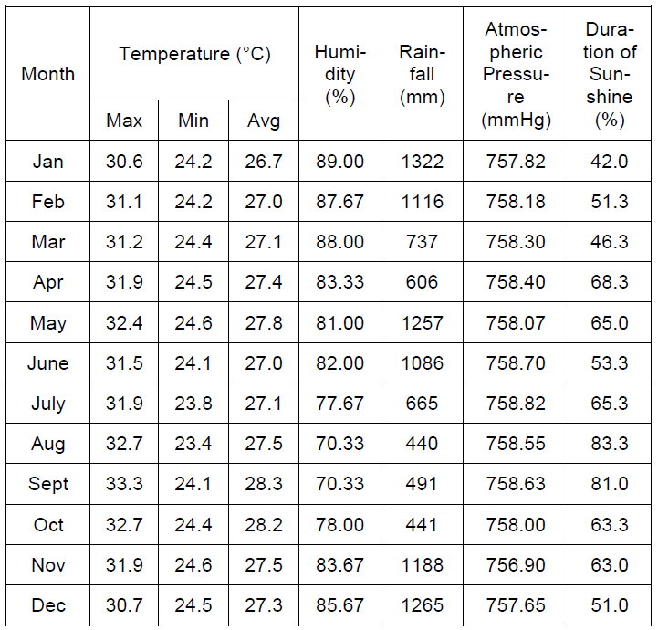
South Sulawesi is a part of Sulawesi Island with an astronomical location in South Sulawesi located at 0 on 12′ South Latitude to 8⁰ North Latitude, and 116⁰ 48′ West Longitude up to 122⁰ 36′ East Longitude. The climate in South Sulawesi is recorded in the South Sulawesi Climatology Station that the temperature throughout 2017 ranges from 23.4 ⁰C – 33.3 ⁰C and the average rainfall is 440 mm to 1322 mm per year. There is significant rainfall in most months of the year. The climatological data are shown in Table 1.

Table 1. Climatology Data of South Sulawesi in 2017 [7]

Analysis Model

In this study, the procedures carried out are:

1) The preparation phase, which is the estimation of what component structure will be used to modeling the corona power losses in the South Sulawesi transmission system.

2) Literature study by studying the literature on modeling loss corona power loss, corona effect on power losses in the transmission system, and also the influence of tropical climate on the large corona power losses that occur in a transmission system.

And 3) Data collection.

Basically, power losses in the transmission network result from transmission lines and transformers at the substation. Transformer loss is the amount of losses in the winding and core losses which are expressed in the form of hysteresis and eddy currents [8]. These losses are released in the form of heat energy. The power losses of the transmission line are very dependent on the magnitude of the network electric current and the losses of the corona phenomenon. In addition, the power losses of the transmission line are affected by changes in the configuration of the electrical system because of the consequences of power outages, maintenance and development of the electrical system. So it is very clear that power losses in transmission lines depends on network parameters, load behavior and climate factors.

Corona power losses generally occur at extra high voltages, in climates that experience low pressure, high temperatures, stormy weather, and rain [9]. This is also the result of a larger conductor size, with a rough and uneven surface which results in a lower critical disruptive voltage. Corona power losses do not occur if the distance between conductors is very large. Therefore, high voltage transmission lines are made with two, three or four conductor bundles where the average geometric radius of the conductor is enlarged.

Furthermore, the loss equation due to the corona in the high voltage transmission line is explained. The corona power losses are expressed by the equation which is the result of research conducted by Peek’s [4]:

where: P_c = transmission line corona power losses (kW / km / phase), δ = relative air density, f = frequency of the electrical system (Hz), r = radius of the transmission line conductor (cm), D = distance between the transmission line conductor (cm), V = phase voltage to neutral transmission line (kV), V_d = critical voltage (kV). In analyzing the influence of tropical climates due to the corona of high voltage air power losses, a relative air density value is needed where the relative air density is affected by the air pressure and the surrounding temperature of the transmission line conductor. The air density equation is shown in equation (2) [10].

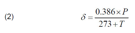
where: δ = relative air density, P = air pressure (mmHg), and T = temperature around the transmission line (°C).

Furthermore, for the disruptive voltage shown in equation (3). Disruptive stress arises due to the emergence of electric field strength due to the collision of electrons in the ionization process. The critical voltage is disruptive considering the influence of conductor factors, conductor and environmental surface uniformity as observed by Peek’s. The critical disruptive voltage value at which the corona begins to form is expressed by:

where: V_d = critical disruptive voltage per transmission line phase (kV), E_c = penetrating air voltage gradient (kV/cm), m = indefinite factor, r = radius of the transmission line conductor (cm), δ = air density relative, and D = distance between transmission line conductors (cm).

The above equations are used in analyzing the influence of tropical climate on the corona power losses at the transmission line in South Sulawesi.

Tropical Climate Effects on Korona Power Losses

Based on the climate data of South Sulawesi, the trend of annual temperature is flat. As with the characteristics of the tropical climate in general, the temperature of each month does not experience large fluctuations. In January, the average temperature was the coldest compared to other months in one year, which was 26.7 °C. While September is the hottest month in a year, with an average temperature of 28.3 °C. From here it can be seen that January is the coldest month, and September is the hottest month.

Corona power loss calculation data based on temperature data for the calculation of average air density per month taken from Table 1 is shown in Fig.2.

Fig.2 shows corona power losses throughout the year based on changes in temperature, where there are graphs based on maximum temperature per month, minimum temperature per month, and average temperature per month. The average corona power losses for the maximum temperature are 2.02 MW, 1.37 MW for the minimum temperature, and 1.63 MW for the average temperature. In the corona power loss chart averaged per month of 275 kV transmission line between Palopo-Makassar, there is no significant increase in corona losses in each month. From Fig.2 also seen in September is the month that has the largest average corona losses of 2.14 MW.

In each corona loss chart throughout the year, the change in the magnitude of the losses is only 0.23 MW for the maximum temperature graph, 0.14 MW for the minimum temperature graph, and 0.12 MW for the average temperature graph.

Seen in Fig.2, the difference in power between maximum temperature and minimum average temperature is 0.65 MW. If the difference in losses occurs all the time, it will cause the operation of the South Sulawesi system to experience fluctuations in the supply of generating power that must be prepared at least equal to the corona losses.

Fig.2. Corona power losses on the 275 kV transmission line in South Sulawesi based on temperature changes

Corona Power Loss Relationships with Humidity

The temperature fluctuations in South Sulawesi are caused by changes in other climatological parameters, namely relative humidity, solar irradiation time, and rainfall. For this reason, it is shown how the relationship between these parameters is to the change in value of corona power losses throughout the year.

The tendency of relative humidity in South Sulawesi in one year is not much different from the air temperature, which is flat, does not experience significant fluctuations. This is mainly seen from the relative relative humidity each month in one year. Table 1 presents the relative relative humidity value, where the highest humidity in January is 89%, while the lowest relative humidity is in September, which is 70.33%.

Fig.3. Graph of corona power losses and relative humidity on 275 kV transmission lines in South Sulawesi

Judging from Fig.3, it is known that the value of corona power losses has a decreased linear with relative humidity values, where corona power losses tend to increase when the relative humidity decreases. The graph of relative humidity relationship with an increase in the value of corona power losses during the year is shown in Fig.4, where the equation y = -0.0033x + 1.8925 with R² = 0.2058, where y = corona (MW) power losses, and x = relative humidity (%). So it can described that when the relative humidity around the transmission system decreases, the value of the corona power losses will be greater. In January, with air humidity of 89%, the value of its power losses was only 1.57 MW.

Whereas when the relative humidity drops to 87.67%, the value of the power losses will be greater, which is 1.59 MW.

Fig.4. Relation of corona power losses and relative humidity on 275 kV transmission lines in South Sulawesi

The Corona Power Loss Relationship with the Duration of Sunshine

Likewise with the sun radiation parameters in a tropical climate. Based on Table 1, the duration of sun exposure in a tropical climate is throughout the day where every day for 12 hours. There are certain months that the duration of the sun’s radiation is slightly disturbed by the presence of clouds, which occurs in January with a figure of 42.0%. While the longest sunshine duration is in August at 83.3%. So it can be ascertained that in August the sky conditions were very bright, only very few clouds covered.

From the graph of the sun irradiation relationship with corona power losses, linear in the same direction is obtained which tends to be the same (Fig.5). The relationship between these two parameters is shown in Fig.6 where the equation based on linear regression is obtained corona losses tend to be directly affected by the duration of sun irradiation in the 275 kV transmission line environment. The equation is y = 0.0018x + 1.513 with R² = 0.2704, where y = corona power losses (MW), and x = solar irradiation time (%).

Fig.5. Graph of corona power losses and duration of sun irradiation on 275 kV transmission lines in South Sulawesi

When the sun shining for a long time around the transmission line, the corona power losses will also be greater. This is because corona power losses are affected by air temperature which affects relative air density. Therefore, when in January the duration of solar radiation was 42%, the value of its power losses (P_c) was only 1.57 MW. Whereas when the duration of sun exposure is 51.3%, the value of its power losses (P_c) will be even greater, which is 1.59 MW.

Based on the relation of relative humidity and duration of sun irradiation in South Sulawesi, a description of these corona power losses can be made, namely the corona power losses are very dependent on the climatic conditions around the transmission line, where the relative humidity decreases and the duration of sun exposure around the transmission line will accelerate the ionization process so that it causes corona. The decrease in humidity and the duration of sun exposure will affect the air pressure around the transmission line.

Fig.6. Relation of corona power losses and the duration of sun circumference on 275 kV transmission lines in South Sulawesi

Corona Power Loss and Rainfall Relation

Because the relative humidity and the duration of the sun irradiation have shown a relationship pattern with corona power losses approaching linear, then it is reviewed how rainfall affects the magnitude of the corona power losses.

Rain occurs almost all year in tropical climates. Table 1 shows that every month in 2017 there is rain in South Sulawesi. Only 4 months in one year that has little rainfall, ie from August to October. The least rainfall is in August with a value of 440 mm. While in other months it has high rainfall. The highest rainfall is in January with a value of 1322 mm.

Fig.7. Graph of corona power losses and rainfall on 275 kV transmission line in South Sulawesi

If the analysis is based on the relation of rainfall graphs and corona power losses (Fig.7), there is no linear relation pattern, where the pattern of rainfall magnitude fluctuates from large to small which produces a non-linear graph trend. In contrast to corona power losses, the graph tends to be linear. Therefore, changes in rainfall values that occur in the South Sulawesi region for one year are not seen to be directly related to the magnitude of the corona power losses. The largest and smallest value of corona power losses occurs not together with the high and low rainfall values in the South Sulawesi. The relationship between the two parameters is shown in Fig.8, where an equation of the results of linear regression is formed which describes corona power losses not directly affected by the amount of rainfall in the 275 kV transmission line environment. The equation is y = -0.0001x + 66.499 with R² = 0.0646, where y = corona losses (MW), and x = rainfall(mm).

However, from the results obtained, it can be described that in high and low rainfall conditions that fluctuate throughout the year it affects air humidity, air temperature and air pressure, so that it can affect the high and low air density factors which make the value of corona losses in the transmission line also change in at that time.

Fig.8. Relationship of corona power losses and rainfall on 275 kV transmission line in South Sulawesi

Conclusion

From the results of the analysis and discussion it can be concluded that the corona power loss (P_c) is directly affected by the temperature and air pressure around the 275 kV transmission line. When the temperature rises, which generally occurs in sunny weather conditions, corona power losses will increase, and vice versa. As a result of temperature changes in South Sulawesi, including tropical climates from the maximum temperature to the minimum temperature, a difference in corona power losses of 0.65 MW can occur throughout the year.

The influence of other tropical climate parameters that are quite dominant affecting corona power losses is the duration of sun exposure. The relationship of the duration of sun irradiation with the value of corona power losses is linearly ascending. Similarly relative humidity also influences the magnitude of corona power losses, which are linearly decreasing. The relative humidity and the rainfall which are also tropical climate parameters connected with the magnitude of the corona power losses in South Sulawesi.

Acknowledgment: The authors gratefully acknowledge Indonesia Government of ministry of research and higher education for financial support of this research.

REFERENCES

[1] Bao-hui, Z., Li-yong, W., Wen-hao, Z., De-cai, Z., Feng, Y., Jinfeng, R., Han, X., Gang-liang, Y., 2005. Implementation of power system security and reliability considering risk under environment of electricity market. IEEE/PES Transmission and Distribution Conference & Exhibition: Asia and Pacific Dalian, China.
[2] ESDM Ministry (Indonesia), 2016. PLN electric power supply business plan for 2016 – 2025. Jakarta.
[3] Yahaya, E.A., Jacob, T., Nwohu, M., Abubakar, A., 2013. Power loss due to corona on high voltage transmission lines. IOSR Journal of Electrical and Electronics Engineering (IOSRJEEE), Vol. 8 No. 3, pp 14-19.
[4] Momani, M.A., 2015. Factors affecting corona power losses in Jordan power grid, 2015 Third International Conference on Technological Advances in Electrical, Electronics and Computer Engineering (TAEECE), IEEE.
[5] Kral, V., Rusek, S., Rudolf, L., 2011. Software for calculation of technical losses in transmission network. Przeglad Elektrotechniczny, R. 87 NR 2, pp 91-93.
[6] Loxton, A.E., Britten, A.C., 2002. The measurement and assessment of corona power losses on 400 kV transmission lines. IEEE Africon.
[7] BPS-Statistics of South Sulawesi, 2018. South Sulawesi province in figures. Makassar, Indonesia.
[8] Masoum, A.S., Moses, P.S., 2011. Distribution transformer losses and performance in smart grids with residential plug-in electric vehicles. ISGT, IEEE.
[9] Liu, Y., You, S., Wan, Q., Lu, F., Chen, W., Chen, Y., 2009. UHV AC corona loss measurement and analysis under rain. Proceedings of the 9th International Conference on Properties and Applications of Dielectric Materials, July 19-23, Harbin, China.
[10] Tonmitr, K., Ratanabuntha, T., Tonmitr, N., Kaneko, E., 2016. Reduction of power loss from corona phenomena in high voltage transmission line 115 and 230 kV. Procedia Computer Science, 86, pp 381 – 384.

Authors: Ikhlas Kitta, Salama Manjang, Ida Rachmaniar, Faris Maricar; Electrical Engineering Department, Hasanuddin University; Makassar, South Sulawesi, Indonesia. Address: Jl. Perintis Kemerdekaan Km.10, 90245. Makassar. E-mail: ikhlaskitta@gmail.com, salamamanjang@gmail.com

Source & Publisher Item Identifier: PRZEGLĄD ELEKTROTECHNICZNY, ISSN 0033-2097, R. 95 NR 1/2019. doi:10.15199/48.2019.01.48

Solving Electric Vehicle Development Challenges

Published by Mark Patrick, EE Power – Technical Articles: Solving Electric Vehicle Development Challenges, July 14, 2022.

A potentially viable approach to solving the development challenges associated with electric vehicles to save both weight and cost.

The growth in EV adoption is a clear and obvious trend, confirmed in several recent industry reports. While the pandemic paused car sales globally, consumers have had time to reflect on their vehicle replacement options, and it appears many are considering an EV as a viable choice. However, many potential obstacles to widespread consumer adoption exist, the most notable being range and charging time anxiety.

Still, thanks to many national and regional government initiatives, and manufacturer special offers, EV sales are set to grow significantly in the coming years.

From the vehicle manufacturer’s perspective, there are still many technical challenges to address moving forward. The initial development of EVs sought to add EV alternatives to existing brand models for the early adopter market. However, sustained and significant growth will require technological advancements on many different fronts.

Battery design, for example, is undergoing major innovation into new chemistries and methods of construction. Although these developments are still in their infancy, there are promising results already. The deployment of a convenient and easy to access EV charging infrastructure requires significant investment too. Range and charging time remain top consumer considerations, along with price, but the key factor impacting these is the vehicle’s weight.

EVs today still maintain a 12 V battery to power non-traction-related functions such as windscreen wipers, seat comfort controls, and infotainment. Some manufacturers are currently replacing a 12 V battery with a 48 V for new models.

The Low Voltage Legacy

Any new vehicle today is equipped with a myriad of electronics-based features, a far cry from when the Hudson Motor Company introduced the concept of a standardized battery in 1918. Today, a sleek touch-controlled infotainment system typically incorporates radio, media players, a GNSS navigation system, smartphone integration, and vehicle status and systems configuration menus. In addition, vehicle occupants can stream music from their smartphone, a high-capacity SD card, or online service. Advanced driver assistance systems (ADAS) use combinations of RADAR, LiDAR, and machine learning-based computer vision to deliver comprehensive driving aids like adaptive cruise control (ACC), blind-spot detection, and emergency braking. The advances in automotive technologies are impressive, but they all share a legacy of the past; the traditional 12 V battery powers them.

For EVs equipped with a 400 V or 800 V battery pack, incorporating an additional battery and the associated power management electronics to power everything highlighted above would appear to incur an unnecessary bill of material cost. Figure 1 illustrates how complex the hybrid and fully EV power architectures have become compared to the internal combustion engine.

In the past, manufacturers packaged individual system functions in separate electronic control units (ECU), each powered with a 12 V supply. This distributed approach to power management and conversion results in high BOM costs. Of course, BOM cost isn’t the only factor to be considered though, since the weight of a 12 V primary battery and all the power components represent a significant payload. For example, the average weight of a 12 V starter battery is 20 kg, which, together with the excess power conversion components, can quickly become significantly increased.

Viewed another way, from the DC/DC power perspective, an electric vehicle power train introduces the need for 50 kW and upwards power conversion and management compared to < 3 kW for a conventional internal combustion engine vehicle. Therefore, achieving reliable and efficient power conversion in the minimum space and with the lowest weight becomes crucial. An EV power architecture needs to support the drive power train, onboard and infrastructure charging, and legacy systems.

Figure 1. A comparison of power architectures used in internal combustion engines, hybrid and fully electric vehicles *(source Vicor). Image used courtesy of Bodo’s Power Systems*

Automotive Power Deliver Architecture; A Different Approach

A viable approach to solving an electric vehicle’s development challenges proposed by Vicor is to use a virtual 12 V (or 24 V/ 48 V) battery (Figure 2). Rather than rely on a separate 12 V battery, why not create a virtual battery directly from the vehicle’s primary 400 V or 800 V battery pack? With this approach, manufacturers can save weight together with a reduction in the associated, engineering, supply chain and stocking costs.

Figure 2. Implementing an EV power architecture with virtual battery 12 V and 48 V sources *(source Vicor). Image used courtesy of Bodo’s Power Systems*

By incorporating high-density HV to LV conversion modules into existing sub-systems, the Vicor approach also achieves a higher degree of integration and a reduction in BoM cost – something OEMs wish to achieve too.

The Vicor proposal focuses on three aspects of the power delivery network architecture illustrated in Figure 2: charging, converting, and delivering.

EV Charging: The EV industry is gradually adopting the 800 V operating voltage for battery packs, but much of the EV charging infrastructure deployed is based on the initial 400 V standard. Therefore, any new EV needs to be able to accommodate both voltage levels. Efficient and straightforward bi-directional conversion modules are already available that offer an extremely flexible, high-efficiency and high-density scalable solution for battery-to-charger station compatibility.

Power Conversion: Conversion of an EV’s primary high voltage battery using a high-density automotive-qualified DC/DC module offers considerable weight and space savings for automotive manufacturers. Again, bi-directional power conversion capabilities provide flexibility in power delivery architectural design. The ability to eliminate the need for a 48 V intermediate energy storage, where used, by a virtual 48 V battery from the HV battery, further provides weight and space savings.

Virtual Power Delivery: In newer vehicles, 48 V applications include new drive, steer and brake-by-wire high power systems. Meeting the power delivery requirements of these networks while supporting legacy 12V loads (see Figure 3) with increased power requirements needs careful consideration. Compact high-density module solutions that are smaller and lighter than legacy solutions are available from Vicor.

Figure 3. Supporting legacy 12 V applications through a virtual power architecture from the vehicle’s HV battery *(source Vicor). Image used courtesy of Bodo’s Power Systems*

Redefining Automotive Power Delivery Architectures

As automotive OEMs grapple with lowering CO₂ emissions while increasing vehicle performance and functionality, electric vehicles are proving to be the best option. However, keeping electric vehicle weight to a minimum to achieve a better range is proving to be a challenge. Redefining the architecture of a vehicle’s power delivery network saves both weight and system costs.

This article originally appeared in Bodo’s Power Systems magazine.

Author: Mark Patrick is Head of Technical Marketing EMEA at Mouser Electronics.

Source URL: https://eepower.com/technical-articles/Solving-Electric-Vehicle-Development-Challenges/

Are You Compliant with the IEEE 519-2022 Edition?

Published by Elspec LTD, website: elspec-ltd.com

The IEEE 519 standard defines the voltage and current harmonics distortion criteria for electrical systems design. The IEEE 519-2022 edition replaces the 2014 edition from December 2022.

The IEEE 519-2022 edition includes two important changes:

• Installations with mixed loads and Inverter Based Resources/Distributed Energy Resources
• Even current harmonics limits

New Guidelines for Installations with Mixed Loads and Inverter Based Resources/Distributed Energy

The 2022 edition instructs you whether to follow the IEEE-519 compliance criteria or different standards, as follows

1. IEEE-519 current limits at the point of common coupling (PCC) should be applied if the installation has an Inverted Based Resources (IBRs) or Distributed Energy Resources (DERs), in addition to the loads, and the combined site rated generation is lower than 10% of the annual average load demand.

2. IEEE 1547 or IEEE 2800 (if applicable) should be applied at the point of common coupling (PCC) should be applied if the installation has an IBRs or DERs, in addition to the loads, and the combined site rated generation is higher than 10% of the annual average load demand.

3. If the installation does not have an IBR or DER, IEEE-519 current limits should be applied at the PCC.

IEEE 519-2022: Even Current Harmonics Limits

The IEEE-519 defines the limits of current distortion per harmonic (in percentages of maximum demand load current) and TDD. The harmonics are divided to 5 groups (3^rd – 10^th, 11^th – 16^th, 17^th – 22^nd, 23^rd – 34^th and 35^th – 50^th), with different limits to each group of harmonics per rated voltage and I_SC/I_L ratio.

In the 2014 edition, all the even current harmonics were limited to 25% of their odd counterparts in their respective harmonic group. The 2022 edition is significantly different since only the even harmonics equal or below the 6^thharmonic are limited, and these harmonics are limited only to 50% of their odd counterparts in the same harmonic group. The meaning is that all the even harmonics above the 6^th harmonics’ values are allowed to be 4 times higher compared to the 2014 edition. i.e., the even harmonics values above the 6^th harmonic can be the same as their odd counterparts in their harmonics group.

This might have a huge impact if you exceed the 2014 standard limits, as you may comply to the 2022 edition, avoiding penalties you might suffer from at the 2014 edition period.

An Example: Current Distortion Limits for Systems Rated 120 V – 69 KV

Table 1. (IEEE 519-2014)

Table 2. (IEEE 519-2022)

Source URL: https://www.elspec-ltd.com/are-you-compliant-with-the-ieee-519-2022-edition/

Understanding the IEEE 519–2014 Standard for Harmonics

Published by Elspec LTD, website: elspec-ltd.com

The IEEE 519-2014 standard defines the voltage and current harmonics distortion criteria for the design of electrical systems. The existed voltage and current waveforms in every part of the system are explained in this standard, and the waveform distortion goals for the system designer are established. The standard is periodically updated as the industry evolves. Since its introduction in 1981, the standard has been updated several times and its latest edition is IEEE 519-2014. Some updates have been made by 2022 (see here). The main terms definitions and statistical evaluation technics are being covered within this current article, as the main changes that have been made in the standard were described in the IEEE-519 2014 edition.

Definitions of Important Terms in the IEEE 519

To understand this document’s aim, the meaning of the following terms applied in this document is written below. The IEEE Standards Dictionary Online should be consulted for other terms not defined below.

1. New Definitions

Maximum demand load current: This current value is enacted at the point of common coupling (PCC) and calculates as the average of the currents corresponding to the peak demand during the previous 12 months.

Notch: A condition, lasting less than ½ cycle, in which the magnitude of the voltage waveform reversed its normal polarity.

Point of common coupling (PCC): the point on a public power supply system, electrically closest to a specific load, other loads are, or maybe connected. The PCC is a point located upstream of the regarded installation.

Illustration 2: Point of common coupling (PCC)

2. Redefined Definitions

Short-circuit ratio: in a specific location, the rate of the available short-circuit current, to the load current, in amperes.

Total demand distortion (TDD): The ratio of the root mean square of the harmonic content, including the harmonic components up-to the 50th order. Expressed as a percent of the maximum demand current. Inter-harmonics are specifically excluded. Higher frequencies (harmonics greater than 50) may be added when required.

Total harmonic distortion (THD): The ratio of the root mean square of the harmonic content, including the harmonic components, up-to the 50^th order. Expressed as a percent of the fundamental. Inter-harmonics are specifically excluded. Higher frequencies (harmonics greater than 50) may be added when required.

3. Legacy definitions

Harmonic (component): An element of order more than one of the Fourier series of a periodic quantity. For instance, in a 60 Hz system, the harmonic order 3, commonly known as the “third harmonic,” is 180 Hz.

Inter-harmonic (component): Refers to the frequency component of a periodic quantity that isn’t an integer multiple of the frequency in which the supply system operates (for instance, 50 Hz or 60 Hz).

I-T product: The inductive influence is expressed as regards the product of the root-mean-square current magnitude (I), in amperes, times its telephone influence factor (TIF).

kV-T product: Inductive influence expressed as regards the product of root-mean-square voltage magnitude (V), in kilovolts, and times its telephone influence factor (TIF).

Notch depth: The average depth of the line voltage notch from the sine wave of voltage.

Notch area: It is the area of the line voltage notch. It is the product of the notch depth, in volts, times the width of the notch measured in microseconds.

Pulse number: The total number of successive non-simultaneous commutations taking place inside the converter circuit during every cycle when operating without phase control. It is also equal to the principal harmonic order in the direct voltage, i.e., the number of pulses available in the dc output voltage in one cycle of the supply voltage.

Telephone influence factor (TIF): For a voltage or recent wave in an electric supply circuit, the ratio of adding the square root of the squares of the weighted root-mean-square values of every one of the sine-wave components (with alternating current waves both fundamental and harmonic) to the root-mean-square value (unweighted) of the whole wave.er loads are, or maybe connected. The PCC is a point located upstream of the regarded installation.

Differences with the Previous Edition

New Measurement Method and Statistical Evaluation Technique

The IEEE 519-2014 introduce a newly measurement methods and statistical evaluation technique to determine compliance with the recommended limits.

Harmonics Measurement Methods

The standard adopt the 10/12 cycles gapless harmonic subgroup measurement from the IEC 61000-4-7. Aggregations of 150/180 cycles (~3sec) and 10min are required for the statistical assessments.

Very short time harmonic measurements: Very short time harmonic values are assessed over a 3-second interval based on an aggregation of 15 consecutive 12 (10) cycle windows for 60 (50) Hz power systems. Individual frequency components are aggregated based on an RMS calculation as shown in Equation (1) where F represents voltage (V) or current (I), n represents the harmonic order, and i is a simple counter. The subscript vs is used to denote “very short.” In all cases, F represents an RMS value.

Short time harmonics measurements: Short time harmonic values are assessed over a 10-minute interval based on an aggregation of 200 consecutive very short time values for a specific frequency component. The 200 values are aggregated based on an RMS calculation as shown in Equation (2) where F represents voltage (V) or current (I), n represents the harmonic order, and i is a simple counter. The subscript sh is used to denote “short.” In all cases, F represents an RMS value.

Statistical Evaluation

Daily evaluation: It is required to calculate the 99^thpercentile value (i.e. the value that is exceeded for 1% of the day) of the very short time harmonics values for comparison with the recommend limits.

Weekly evaluation: It is required to calculate the 95^th and 99^th percentile value (i.e. those values that are exceeded for 5% and 1% of the week) of the short time harmonics values for comparison with the recommend limits.

The chart below display a daily accumulative and relative probability chart of the Total Demand Distortion parameter at resolution of 3sec as taken from PQSCADA Sapphire.

The IEEE 519 – 2014 Compliance Criteria

These suggested practice limits are for application at a point of common coupling (PCC) between the system owner or operator and system users. The PCC is often regarded as the point in the power system closest to the user where the system owner or operator could provide services to other users. Usually for service to industrial users, e.g., manufacturing plants through a unique service transformer, the PCC will be at the transformer’s HV side. For most commercial users like office parks, etc., supplied through a usual service transformer, the PCC is commonly at the LV side of the service transformer.

Voltage Distortion Limits

• Daily 99^thpercentile very short time (3 s) values should be less than 1.5 times the values given in the table below.

• Weekly 95^thpercentile short time (10 min) values should be less than the values given in the table below.

Table 1. (IEEE 519-2014)

Current Distortion Limits

• Daily 99^th percentile very short time (3 s) harmonic currents should be less than 2.0 times the values given in the tables below.

• Weekly 99^th percentile short time (10 min) harmonic currents should be less than 1.5 times the values given in tables below.

• Weekly 95^th percentile short time (10 min) harmonic currents should be less than the values given in tables below.

Table 2. (IEEE 519-2014) Current distortion limits for systems rated 120 V – 69 kV

Table 3. (IEEE 519-2014) Current distortion limits for systems rated 69 kV – 161 kV

Table 4 (IEEE 519-2014) Current distortion limits for systems rated > 161 kV^a

^a Even harmonics are limited to 25% of the odd harmonic limits above
^b Current distortions that result in a dc offset, e.g., half-wave converters, are not allowed
^c All power generation equipment is limited to these vales of current distortion, regardless of actual I_SC/I_L.
I_SC = maximum short circuit current at PCC
I_L = maximum demand load current (fundamental frequency component) at PCC

Source URL: https://www.elspec-ltd.com/ieee-519-2014-standard-for-harmonics/

Assessment of the Impact of the Micro Wind Turbine on the Power Quality in the Distribution Network

Published by Marek GAŁA, Andrzej JĄDERKO, Politechnika Częstochowska, Wydział Elektryczny

Abstract. The article presents the principles of measurements and assessment of power quality characteristics, with the power supplied by the micro wind turbine connected to the distribution network. It describes the basic technical parameters of the vertical axis micro wind turbine 10 kW and the characteristics of its output as a function of wind speed. Besides, it shows selected results of measurements of parameters characterizing the power quality in the node of micro wind turbine of 10 kW connection to the 400 V network.

Streszczenie. W artykule przedstawiono zasady pomiarów i oceny jakości energii dostarczanej przez mikroturbinę wiatrową podłączoną do sieci dystrybucyjnej. Opisano podstawowe parametry techniczne mikroturbiny wiatrowej o pionowej osi obrotu i mocy 10 kW oraz charakterystykę jej mocy wyjściowej w funkcji prędkości wiatru. Pokazano również wybrane wyniki pomiarów parametrów charakteryzujących jakość energii w węźle przyłączenia mikroturbiny wiatrowej do sieci dystrybucyjnej 400 V. (Ocena wpływu pracy mikroturbiny wiatrowej na jakość energii elektrycznej w sieci dystrybucyjnej niskiego napięcia).

Keywords: vertical micro wind turbine, power quality, distribution network
Słowa kluczowe: mikroturbina wiatrowa o pionowej osi obrotu, jakość energii, sieć dystrybucyjna

Introduction

The current regulations applicable to non-business energy users state that a microgeneration plant can be connected free of charge to the distribution grid after reporting such an intention to a regional distribution company. Additionally, various funds can be obtained to finance investments into Renewable Energy Sources (RES). These factors are responsible for the visibly growing interest in RES, especially photovoltaic systems and wind turbines, equipped with inverter systems, control systems and protection systems [1, 2, 12].

The massive increase in the number of microgeneration plants can however cause significant problems for the distribution grid, including aggravation of energy quality. Because of this, microgeneration plants connected to the grid should meet a number of technological requirements, as well as conditions specified by grid operators in the relevant instructions, e.g. [9] and [3], in accordance to applicable standards and regulations [4, 5, 6, 10].

In the next sections of this paper characteristics of the wind turbine MEW-10 are presented, followed by selected measurement results of electrical energy quality generated by this unit.

Characteristic of a wind turbine

The wind turbine type MEW-10 consists of a vertical axis wind turbine (VAWT) with a three-blade rotor of the H-Darrieus type, a disc slow-rotation permanent magnet synchronous generator (PMSG) and a controller together with protection systems. The rated power obtained by the wind speed 12 m/s is 10 kW. If the wind speed exceeds this value, the power is constrained by the control system [11]. The maximal rotational speed of the rotor is about 140 rpm. A number of empirically obtained characteristics of the MEW-10 are presented in Table 1.

Table 1. Basic characteristics of the MEW-10 wind turbine

The cross-section area of the rotor (wind circle) is 30 m², with the blade height of 6 m and the rotor diameter of 5 m. A blade cross-section is a symmetrical assembly of standard airfoils type NACA 0021. A wind turbine of the type investigated in the paper is presented in Figure 1.

A power inverter creates current load on the plant generator, which causes torque on the shaft, adjusting the rotational turbine speed to the current wind speed, in this way ensuring the maximal power coefficient. A grid-tie inverter couples the generator with the power grid, generating three voltage waveforms synchronized with the grid phase voltages.

Fig.1. Vertical wind turbine of type MEW-10

Measurements of the quality of wind turbine-generated energy

The measurements of energy quality at a connection node of the wind turbine in an consumer internal grid were carried out in the first half of July 2018, by means of an energy quality analyzer PQ-Box 200, meeting the requirements of the standard [8] with respect to class A. The measurements were intended to verify if energy generated by the wind turbine meets the requirements specified in [3, 4, 5, 9]. Below are presented selected results of power parameters and energy quality parameters collected over a week period of observation, with a 10- minute period of data aggregation, t_A = 600 s.

Figure 2 presents the mean square (rms) values of phase current, the maximum value of which was I_max= 3.3A, and the rms value at t_A = 0.2 s was I_{max 0.2s} = 12.23 A. The visible asymmetry of currents is caused by the current I_inv = 0.29 A flowing through the power inverter control system from the phase L₃. Figure 3 presents the values of the active power P and the reactive power Q. The minimal value of the active power was P_min= -1,8 kW (P_{min 0.2s} = – 8,66 kW – the case of maximum power generation by the wind turbine). The working inverter consumes the power of about P_inv= 37.5 kW. As can be seen, the plant has significant demand for reactive power: Q_min= -1,5 kvar (Q_{min 0.2s} = -5,44 kvar) – Fig. 3.

Fig.2. Root mean square values of the currents *I_L1*, *I_L2*, *I_L3* at the node connection node

Fig.3. Active power P and reactive power Q of micro wind turbine during one week of measurements

Figure 4 presents the values of voltage THD coefficients. No voltage distortion exceeding the admissible level was observed: THD U ∊ 〈1.88, 3.05〉%.

Fig.4. *THD U_L1*, *THD U_L2*, *THD U_L3* of phase voltage in the node of micro wind turbine

Figure 5 presents the momentary currents recorded at maximal power generation, i.e. P = P_min. The current deformation was assessed by obtaining harmonic rms values for n = 2,…,50 and comparing them to the values specified in the relevant standards [4, 6]. The results obtained are presented in Table 2. As can be noted, the plant does not cause higher harmonics of values exceeding the admissible limit level to flow through the connection node of the wind turbine.

Fig.5. Momentary values of currents *I_L1*, *I_L2*, *I_L3* at *P_min*

Table 2. Comparison of the measured results of higher harmonics with values specified in the standard

The value of THD I for P_min was THD I_Pmin = 7.11%. Curves representing the variation of the voltage and current asymmetry coefficients were obtained on the basis of the direct components (U₁, I₁) and inverse components (U₂, I₂):

Figure 6 presents the voltage coefficient curve. With the maximal value of the coefficient α_Umax = 0.32%, it is significantly smaller than the limit value of 2%. It was also observed that the value of current asymmetry coefficient varies from 1.78% at P_min to 100% when no power is generated and only the phase L₃ is under load due to the power inverter being powered from this circuit. Figure 7 presents the variation of the indices P_lt The values of the index P_lt are within the interval 0.25 – 0.50, whereas the values of the index P_st are included in the interval 0.07 – 0.67. According to [8], the values of the indices P_st and P_ltdo not exceed the limit values, as specified in [3]:

Fig.6. Voltage asymmetry coefficient *α_U*

Fig.7. Indices of long-term flicker severity *P_{lt L1}*, *P_{lt L2}*, *P_{lt L3}* in the node of micro wind turbine

The power inverter control system requires continuous supply of active energy E₊ (blue), even when it is working at wind speeds below the turbine start-up speed. The amount of active energy consumed during the test week was 5,36 kWh and the amount of reactive energy was E_Q (purple) (7.50 kvarh) – Fig. 8. The total net amount of energy supplied to the grid was E₊= 2.08 kWh (green), but is has to be kept in mind that the measurements were taken during summer, and the wind speed attested at that time was not optimum for the operation of the wind turbine.

Fig.8. Energy: E – active energy supplied to the grid (red), E₊ – active energy consumed by the power inverter (blue), E₊ – active energy generated by the wind turbine plant (green); E_Q– reactive energy consumed from the grid by the wing turbine plant (purple)

In order to analyze in detail the plant’s demand for reactive power, additional measurements were carried out, with the consideration of the aggregation time t_A = 1 s – Fig. 9. Besides, Figures 10 and 11 present momentary values of currents and voltages, respectively, during the charging of capacitors in the intermediary circuit of the power inverter in the microgeneration plant.

Fig.9. Current I, active power P and reactive power Q during the charging of the capacitors in the power inverter intermediary circuit; *t_A* = 1 s

Fig.10. Momentary currents *I_L1*, *I_L2*, *I_L3* during connecting capacitors into the intermediary power inverter circuit

Fig.11. Momentary voltages *U_L1*, *U_L2*, *U_L3* during connecting capacitors into the intermediary power inverter circuit

Conclusions

The measurements carried out for the sake of the present study indicate that the operation of the wind turbine does not cause voltage changes exceeding 3%, nor does it cause voltage asymmetry, voltage fluctuations or current harmonics exceeding admissible limit levels. During the charging of the capacitors in the power inverter circuit, impulse currents with momentary values reaching 90 A occurred, which caused additional voltage drop at the grid impedance and contributed to momentary voltage distortion, as shown in Fig. 11. This phenomenon was not however found to interfere with the operation of any devices at the consumer side. Still, it needs to be further scrutinized by the manufacturer of the power inverter with the view to optimizing the control algorithm. Besides, another set of verification measurements should be carried out at wind speeds ensuring generating the rated power of the wind turbine.

REFERENCES

[1] Act on Power Law of 10 April 1997, Journal of Laws of 1997 no 54, item 348, with later amendments (Ustawa z dnia 10 kwietnia 1997 r. Prawo energetyczne, Dz. U. z 1997 r., nr 54, poz. 348 z późn. zm.).
[2] Act on Renewable Energy Sources of 20 February 2015, Journal of Laws of 2015, item 478 (Ustawa z dnia 20 lutego 2015 r. o odnawialnych źródłach energii (Dz. U. z 2015 r., poz. 478).
[3] Connection criteria and technical requirements for microgeneration plants and small-scale generation plants connected to the LV distribution network (Kryteria przyłączania oraz wymagania techniczne dla mikroinstalacji i małych instalacji przyłączanych do sieci dystrybucyjnej niskiego napięcia) TAURON Dystrybucja S.A., Krakow, July 18, 2016
[4] EN 50438 Requirements for micro-generating plants to be connected in parallel with public low-voltage distribution networks
[5] IEC 61000-3-2:2014 Electromagnetic compatibility (EMC) – Part 3-2: Limits – Limits for harmonic current emissions (equipment input current ≤ 16 A per phase).
[6] IEC 61000-4-7:2002+A1:2008 Electromagnetic compatibility (EMC) – Part 4-7: Testing and measurement techniques – General guide on harmonics and interharmonics measurements and instrumentation, for power supply systems and equipment connected thereto.
[7] IEC 61000-4-15:2010 Electromagnetic compatibility (EMC) – Part 4-15: Testing and measurement techniques – Flickermeter Functional and design specifications.
[8] IEC 61000-4-30:2015 Electromagnetic compatibility (EMC) – Part 4-30: Testing and measurement techniques – Power quality measurement methods.
[9] Instructions for Distribution Network Traffic and Exploitation applicable since 01.01.2014, TAURON Dystrybucja S.A. (Instrukcja Ruchu i Eksploatacji Sieci Dystrybucyjnej TAURON Dystrybucja S.A. obowiązująca od dnia 01.01.2014 r.).
[10] The Ministry of Economy ordinance on the detailed conditions of the power system operation, Journal of Laws of 2007, no, 93, item 623 with later amendments (Rozporządzenie Ministra Gospodarki z dnia 4 maja 2007 r. w sprawie szczegółowych warunków funkcjonowania systemu elektroenergetycznego, Dz. U. z 2007 r., nr 93, poz. 623 z późn. zm.).
[11] Turbine MEW-10 catalogue description
[12] Sobierajski M., Rojewski W. ”Conditions for connecting microgeneration plants to the LV grid vs. legal regulations,” (Warunki przyłączania mikrogeneracji do sieci niskiego napięcia w świetle obowiązujących przepisów), Zeszyty Naukowe Wydziału Elektrotechniki i Automatyki Politechniki Gdańskiej, nr 33/2016, pp. 79-82

Authors: dr inż. Andrzej Jąderko, Politechnika Częstochowska, Wydział Elektryczny, Al. Armii Krajowej 17, 42-200 Częstochowa, e-mail: aj@el.pcz.czest.pl
dr inż. Marek Gała, Politechnika Częstochowska, Wydział Elektryczny, Al. Armii Krajowej 17, 42-200 Częstochowa, e-mail:m.gala@el.pcz.czest.pl

Source & Publisher Item Identifier: PRZEGLĄD ELEKTROTECHNICZNY, ISSN 0033-2097, R. 95 NR 1/2019. doi:10.15199/48.2019.01.09

HARMONICS: Understanding the Facts – Part 3

Published by Richard P. Bingham

Abstract. Understanding what is important to know about harmonics can be challenging for those without extensive electrical engineering backgrounds. This is third and final part of a three part series. This part will provide details on what causes harmonic problems and suggested solutions.

What they look like

One recent survey showed the percentage the total electrical consumption by non-linear loads will double from the year 1985 to 2000. The AC-DC converter used in the switching-type power supplies found in most personal computers and peripheral equipment, such as printers, is an example of a non-linear load. While they offer many benefits in size, weight and cost, the large increase of equipment using this type of power supply over the past fifteen years is largely responsible for the increased attention to harmonics.

Figure 1 shows how the first stage of a switching-type power supply works. The AC voltage is converted into a DC voltage, which is further converted into other voltages that the equipment needs to run. The rectifier consists of semi-conductor devices (such as diodes) that only conduct current in one direction. In order to do so, the voltage on the one end must be greater than the other end. These devices feed current into a capacitor, where the voltage value on the capacitor at any time depends on how much energy is being taken out by the rest of the power supply.

\When the input voltage (V_i) is higher than voltage on the capacitor (V_c), the diode will conduct current through it. This results in a current waveform as shown in Figure 2, and harmonic spectrum in Figure 3. Obviously, this is not a pure sinusoidal waveform with only a 60 Hz frequency component.

Figure 3. Harmonic Spectrum of Current Waveform Shown in Figure 2. If the rectifier had only been a half-wave rectifier, the waveform would only have every other current pulse, and the harmonic spectrum would be different. Whereas the above harmonic spectrum contains only odd harmonics for current, the spectrum for the current of a half wave rectified circuit would only have even harmonics.

Certain types of loads also generate typical harmonic spectrum signatures, that can point the investigator towards the source. This is related to the number of pulses, or paths of conduction. The general equation is h = ( n*p ) +/- 1, where h is the harmonic number, n is any integer (1,2,3,..) and p is the number of pulses in the circuit. Table 1 shows examples of such. The magnitude decreases as the ratio of 1/h (1/3, 1/5, 1/7, 1/9,…).

Table 1. Typical Harmonics Found for Different Converters.

When transformers are first energized, the current drawn is different from the steady state condition. This is caused by the inrush of the magnetizing current. The harmonics during this period varies over time. Some harmonics have a negligible value for part of the time, and then increase for a while before returning to basically zero. An unbalanced transformer (where either the output current, winding impedance, or input voltage on each leg are not equal) will cause harmonics, as will overvoltage saturation of a transformer.

Fluorescent lights can be the source of harmonics, as the ballasts are non-linear inductors. The third harmonic is the predominate harmonic in this case. (See Table 2) As previously mentioned, the third harmonic current from each phase in a four-wire wye or star system will be additive in the neutral, instead of canceling out Some of the newer electronic ballasts have very significant harmonic problems, as they operate somewhat like a switching power supply, but can result in current harmonic distortion levels over 30%.

Table 2. Sample of Harmonic Values for Fluorescent lighting [4].

The process of melting metal in an electric arc furnace can result in large currents that are comprised of the fundamental, interharmonic, and subharmonic frequencies being drawn from the electric power grid. These levels can be quite high during the melt-down phase, and usually effect the voltage waveform.

How do you get rid of them

Care should be undertaken to make sure that the corrective action taken to minimize the harmonic problems don’t actually make the system worse. This can happen as the result of resonance between harmonic filters, PF correcting capacitors and the system impedance. Examples of ways to minimize the harmonic problems include:

• Isolating harmonic pollution devices on separate circuits with or without the use of harmonic filters. – Loads can be relocated to try to balance the system better.

• Phase shifted transformers, such as “zig-zag transformers”, can be used to cancel out specific harmonics by making one voltage circuit 180 degrees out-of-phase from another.

• Neutral conductors should be properly sized according to the latest NEC-1996 requirements covering such. Where as the neutral may have been undersized in the past, it may now be necessary to run a second neutral wire that is the same size as the phase conductors. This is particularly important with some modular office partition-type walls, which can exhibit high impedance values.

• The operating limits of transformers and motors should be derated, in accordance with industry standards from IEEE, ANSI and NEMA on such.

• Use of higher pulse converters, such as 24-pulse rectifiers, can eliminate lower harmonic values, but at the expense of creating higher harmonic values.

Summary

Harmonics are here to stay. But the amount of harmonic voltage and current levels that a system can tolerate is dependent on the equipment and the source. Ongoing preventive maintenance programs that include harmonic monitoring can detect problems in the making, eliminating costly failures. Knowing what your system harmonic levels presently are, what the effect of new equipment being added will due to these levels, and how much of an increase in harmonic levels that your system can tolerate are valuable pieces of information that are readily attainable from modern power quality/harmonic analyzer monitoring equipment.

References

National Electrical Code – NEC-1996, National Fire Protection Association

Blog posts:
HARMONICS: Understanding the Facts – Part 1,
HARMONICS: Understanding the Facts – Part 2

HARMONICS: Understanding the Facts – Part 2

Published by Richard P. Bingham

Abstract. Understanding what is important to know about harmonics can be challenging for those without extensive electrical engineering backgrounds. In this two part series, this second article will help to clarify why you need to be concerned about them, how and where to find them, and when they are a problem.

Why Worry About Harmonics

The presence of harmonics does not mean that the factory or office cannot run properly. Like other power quality phenomena, it depends on the “stiffness” of the power distribution system and the susceptibility of the equipment when operating in the presence of the harmonics. One factory may be the source of high harmonics but be able to operate properly. This harmonic pollution is often carried back onto the electric utility distribution system, and may effect neighboring facilities on the same system which are more susceptible.

There are a number of different types of equipment that may experience misoperations or failures due to high harmonic voltage and/or current levels:

• Excessive neutral current, resulting in overheated neutrals. The currents of triplen harmonics, especially the odd harmonics, (3^rd, 9^th, 15^th,…) are actually additive in the neutral of three phase wye circuits. This is because the harmonic number multiplied by the 120 degree phase shift between the three phases is a integer multiple of 360 degrees, or one complete cycle. This puts the harmonics from each of the three phase conductors “in-phase” with each other in the neutral, as shown in Figure 1.

• Incorrect reading meters, including induction disc-type W-hr meters and averaging type current meters.

• Reduced true PF, where PF= Watts/VA.

• Overheated transformers, especially delta windings where triplen harmonics generated on the load side of a delta-wye transformer will circulate in the primary side. Some type of losses go up as the square of harmonic value (such as skin effect and eddy current losses). This is also true for solenoid coils and lighting ballasts.

• Positive, negative, and zero sequence voltages on motors and generators. These are voltages at a particular frequency that try to rotate the motor forward, backward, or neither (just heats up the motor), respectively. As shown in Table 1, the voltage of a particular frequency in a balanced system harmonics can have either a positive (fundamental, 4^th, 7^th,…), negative (2^nd, 5^th, 8^th…) or zero (3^rd, 6^th, 9^th,…) sequencing value.

Table 1. Harmonic Sequencing Values in Balanced Systems.

• Nuisance operation of protective devices, including false tripping of relays and failure of a UPS to transfer properly, especially if the controls incorporate zero-crossing sensing circuits.

• Bearing failure from shaft currents through uninsulated bearings of electric motors.

• Blown-fuses on PF correction caps, due to high voltage and currents from resonance with line impedance.

• Mis-operation or failure of electronic equipment – Light flicker results when there are voltage subharmonics in the range of 1-30Hz. The human eye is most sensitive at 8.8Hz, where just a 0.5% variation in the RMS voltage is noticeable with some types of lighting.[2]

Where They Come From

The amount of voltage harmonics will often depend on the amount of harmonic currents being drawn by the load, and the source impedance, which includes all of the wiring and transformers back to the source of the electricity. Ohm’s Law says that Voltage equals Current multiplied by Impedance. This is true for harmonic values as well. If the source harmonic impedance is very low (often referred to as a “stiff” system) then the harmonic currents will result in lower harmonic voltages than if the source impedance were high (such as found with some types of isolation transformers). The impedance of an inductive device goes up as the frequency goes up, while the impedance goes down for capacitive devices for higher harmonics.

How this electricity is used by the different types of loads can have an effect on the “purity” of the voltage waveform. Some loads cause the voltage and current waveforms to lose this pure sine wave appearance and become distorted. Depending on the type of load and system impedances, the waveform may consist of predominately harmonics.

“The main sources of harmonic current are at present the phase angle controlled rectifiers and inverters.” [3] These are often called static power converters. These devices take AC power and convert it to DC, then sometimes back to AC power at the same or different frequency based on the firing scheme. The firing scheme refers to the controlling mechanism that determines how and when current is conducted. One major variation is the phase angle at which conduction begins and ends.

Power converters come in different sizes. Low power, AC voltage regulators for light dimmers and small induction motors adjust the phase angle or point on the wave where conduction occurs. Medium power converters are used for motor control in manufacturing and railroad applications, and include such equipment as ASDs (adjustable speed drives) and VFDs (variable frequency drives). Metal reduction operations, like electric arc furnaces, and high voltage DC transmission employ large power converters, in the 2-20MVA rating.

Where to look for them

Wherever the aforementioned equipment is used, one can suspect that harmonics are present. Like any power quality investigation, the search can begin at the equipment effected by the problem or at the point-of-common-coupling (PCC), where the utility service meets the building distribution system. If only one piece of equipment is effected (or suspected as being the producer), it is often easier to start the monitoring process there. If the source is suspected to be from the utility service side (such is the case when there is a neighboring factory that is known to generate high harmonics), then monitoring usually begins at the PCC.

How do you find them

Hand-held harmonic meters can be useful tools for making spot checks for known harmonic problems. However, harmonic values will often change during the day, as different loads are turned on and off within the facility or in other facilities on the same electric utility distribution system. This requires the use of a harmonic monitor or power quality monitor with harmonic capabilities (such as shown in Figure 2), which can record the harmonic values over a period of time.

Figure 2. Power Quality Monitor with Harmonic Analysis

The phase voltages and currents, as well as the neutral-to-ground voltage and neutral current should be monitored, where possible. This will aid in pinpointing problems, or detecting marginal systems. Monitoring the neutral will often show a high 3rd harmonic value, indicating the presence of non-linear loads in the facility.

Typically, monitoring will last for one business cycle. A business cycle is how long it takes for the normal operation of the plant to repeat itself. For example, if a plant runs three identical shifts, seven days a week, then a business cycle would be eight hours. More typically, a business cycle is one week, as different operations take place on a Monday, when the plant equipment is restarted after being off over the weekend, then on a Wednesday, or a Saturday, when only a skeleton crew may be working.

In order to be able to analyze complex signals that have many different frequencies present, a number of mathematical methods were developed. One of the more popular is called the Fourier Transform. Duplicating the mathematical steps required in a microprocessor or computer-based instrument is quite difficult. So more compatible processes, called the FFT for Fast Fourier Transform, or DFT for Discrete Fourier Transform, are used. These methods only work properly if the signal is composed of only the fundamental and harmonic frequencies in a certain frequency range (called the Nyquist frequency, which is one-half of the sampling frequency). The frequency values must not change during the measurement period. Failure of these rules to be maintained can result in mis-information.

For example, if a voltage waveform is comprised of 60Hz and 200Hz signals, the FFT cannot directly see the 200Hz. It only knows 60, 120, 180, 240,…, which are often called “bins”. The result would be that the energy of the 200Hz signal would appear partially in the 180Hz bin, and partially in the 240Hz bin. An FFT-based processer could show a voltage value of 115V at 60Hz, 18V at the 3^rd harmonic, and 12V at the 4^th harmonic, when it really should have been 30V at 200Hz. A spectrum analyzer can also exhibit a similar problem, as it places the energy in its own machine-dependent bins. In addition, a spectrum analyzer takes only a snap-shot in time of the harmonics, which are best analyzed on an averaged, steady-state waveform.

When are they a problem

To determine what is normal or acceptable levels, a number of standards have been developed by various organizations. ANSI/IEEE C57.110 Recommended Practice for Establishing Transformer Compatibility When Supplying Non-sinusoidal Load Currents [5] is a useful document for determining how much a transformer should be derated from its nameplate rating when operating in the presence of harmonics. There are two parameters typically used, called K-factor and TDF (transformer derating factor). Some power quality harmonic monitors will automatically calculate these values.

IEEE 519-1992 Recommended Practices and Requirements for Harmonic Control in Electrical Power Systems [6] provides guidelines from determining what are acceptable limits. The harmonic limits for current depend on the ratio of Short Circuit Current (SCC) at PCC (or how stiff it is) to average Load Current of maximum demand over 1 year, as illustrated in Table 2. Note how the limit decreases at the higher harmonic values, and increases with larger ratios.

Table 2. Current Harmonic Limits as per IEEE 519-1992.

For voltage harmonics, the voltage level of the system is used to determine the limits, as shown in Table 3. At the higher voltages, more customers will be effected, hence, the lower limits.

Table 3. Voltage Harmonic Limits as per IEEE 519-1992.

The European Community has also developed susceptibility and emission limits for harmonics. Formerly known as the 555-2 standard for appliances of less than 16 A, a more encompassing set of standards under IEC 1000-4-7 are now in effect.

Most electrical loads (except half-wave rectifiers) produce symmetrical current waveforms, which means that the positive half of the waveform looks like a mirror image of the negative half. This results in only odd harmonic values being present. Even harmonics will disrupt this half-wave symmetry. The presence of these even harmonics should cause the investigator to suspect there is a half-wave rectifier on the circuit. This also result from a full wave rectifier when one side of the rectifier has blown or damaged components. Early detection of this condition in a UPS system can prevent a complete failure when the load is switched onto back-up power.

References

[1] Power Line Harmonic Problems – Causes and Cures, Dranetz Technologies, December 1994.
[2] NFPA 70B Recommended Practice for Electrical Equipment Maintenance – Chapter
24, National Fire Protection Association, Quincy MA, 1994.
[3]J. Arrillega et.al. Power System Harmonics, John Wiley and Sons, 1985.
[4]Heydt, GT, Electric Power Quality, Stars in the Circle Publication, Indianapolis, 1991, pg 240.
[5] ANSI/IEEE C57.110 Recommended Practice for Establishing Transformer Compatibility When Supplying Nonsinusoidal Load Currents
[6] IEEE 519-1992 Recommended Practices and Requirements for Harmonic Control in Electrical Power Systems National Electrical Code – NEC-1996, National Fire Protection Association

About the Author: Richard P. Bingham is currently the Chief Technologist for Dranetz Technologies, Inc., having previously been the Vice-President of Engineering and Strategic Planning. He has been with the company since 1977, following completion of his BSEE at the University of Dayton. Richard also has an MSEE in Computer Architecture and Programming from Rutgers University. He is a member of IEEE Power Engineering Society and Tau Beta Pi, the Engineering Honor Society. Richard is currently working with the NFPA 70B committee on Power Quality and several IEEE committees related to IEEE 1159, and has written and presented numerous papers and seminars in the electric utility and power quality instrumentation fields.

Blog post: HARMONICS: Understanding the Facts – Part 1

HARMONICS: Understanding the Facts – Part 1

Published by Richard P. Bingham

Abstract. Understanding what is important to know about harmonics can be challenging for those without extensive electrical engineering backgrounds. In this three part series, this first article will review what a harmonic is, the second will help to clarify what those important facts are, and the third will provide details on what causes harmonic problems and suggested solutions.

Why a Sine Wave

Before defining what a harmonic is, it is useful to review why electrical power is generated in the form of a sine wave, as shown in Figure 1. In much of the world, an AC generator is used to produce power. AC, or alternating current, was chosen back in the 1800s over DC, or direct current, due to its ease of generation and the ability to change amplitude using transformers. [1] The key to understanding a sine wave is in understanding what it is that is “alternating.”

The principle in most AC generators is that by rotating a magnetic field over coils or windings, an alternating electric current will be induced into the windings. The current (or electrical force) is proportional to the magnetic flux (magnetic force), and the voltage (electrical potential) is proportional to the rate of change of the current. If there was no change or alternating of the magnetic flux and hence no change in the current, then there would be no voltage produced.

A mechanical force, such as water, steam or wind, is used to provide the rotation to produce this changing flux. Figure 2 is a cross-section of a three phase, 2 pole generator. Half of the windings for each phase are located on opposite sides of the stator, or stationary part of the generator. When these coil pairs (A+/A-, B+/B-, C+/C-) are joined together, the current can flow through the circuit of the windings. In the center is the magnet, which has a north and south pole. The magnetic flux gets stronger as the rotating pole gets closer to the coil, and then reduces in intensity as it goes past. The north pole makes the current flow into one coil and the south makes it flow out of the other. In some generators, the magnets are actually electromagnets, not permanent magnets.

Figure 2. Cross section of three phase, two pole generator.

Why the voltage is a sine wave is best illustrated by looking at the phasor diagrams in Figure 3. As the phasor rotates around the circle (like the magnets rotating inside the generator), the position of the end of the phasor in the y axis is shown in Table 1. This is done in 15 degree steps in this example to save space.

Table 1. Phase Angle and Magnitude values

Position	Phase Angle	Y axis value
A	0 degrees	0
B	15 degrees	0.259
C	30 degrees	0.5
D	45 degrees	0.707
E	60 degrees	0.866
F	75 degrees	0.966

The rotational position (in degrees) is related to an incremental step in time. Plotting the y axis values corresponding to the position steps over a complete 360 degree circle results in an approximation of a sine wave that was shown in Figure 1. This sine wave function occurs in many natural phenomena, such as the speed of a pendulum as it swings back and forth, or the way a string on a guitar vibrates when plucked.

The frequency of the sine wave is proportional to the number of poles (or magnets) and the speed of the rotation, usually expressed in ‘rpm’ (revolutions per minute). The equation is f = ( p/2 )*rpm. This frequency is referred to as the fundamental frequency. In the North America, this frequency is 60Hz, or cycles per second. In European countries and other parts of the world, this frequency is usually 50Hz. Aircraft often use 400Hz as the fundamental frequency. At 60Hz, this means that sixty times a second, the voltage waveform increases to a maximum positive value, then decreases to zero, further decreasing to a maximum negative value, and then back to zero.

What is a Harmonic

The knowledge of harmonics has been around for a long time. In fact, musicians have been aware of such since the invention of the first string or woodwind instrument. Harmonics (called “overtones” in music) are responsible for what makes a trumpet sound like a trumpet, and a clarinet like a clarinet. It can be shown that any complex waveform, whether it is produced by a musical instrument or a power system, can be broken up into harmonic components.

The typical definition for a harmonic is “a sinusoidal component of a periodic wave or quantity having a frequency that is an integral multiple of the fundamental frequency.” [2]. Some references refer to “clean” or “pure” power as those waveforms without any harmonics. Today, such clean waveforms typically only exist in a laboratory.

The harmonic frequencies are integer multiples [2, 3, 4, …] of the fundamental frequency. For example, the 2nd harmonic on a 60Hz system is 2*60 or 120Hz. At 50Hz, the second harmonic is 2*50 or 100Hz. 300Hz is the 5^th harmonic in a 60Hz system, or the 6^th harmonic in a 50Hz system. Figure 5 shows how a signal with dominant 5^th and 7^th harmonics would appear on an oscilloscope-type display, which some power quality analyzers provide.

Figure 5. Fundamental with 5^th and 7^th harmonics

Frequencies that are not integer multiples of the fundamental frequency are called “interharmonics ”. There is also a special category of interharmonics, which are frequency values less than the fundamental frequency, called subharmonics. The presence of sub-harmonics is often observed by the lighting flicker.

One other parameter to be aware of is the phase angle of the harmonic relative to the fundamental. In Figure 6, a third harmonic with an amplitude of 33% of the fundamental is combined with the fundamental. In the left hand picture, the fundamental and the third harmonic are in phase. In the right hand picture, they are 180 degrees out-of-phase with each other. Obviously, the resulting waveform looks quite different.

References

[1] Fitzgerald, A.E. et al, Electric Machinery, McGraw-Hill Company, 1971.
[2] IEEE 519 Recommended Practices and Requirements for Harmonic Control in Electric Power Systems
[3] Kerchner, Russel M. And George F. Corcoran, Alternating-Current Circuits, John Wiley & Sons, NY, 1 943.
[4] Powerline Harmonic Problems – Causes and Cures, Dranetz Technologies, December 1994.

Comparison of PV Plant Energy Generation Prediction Tools with Measured Data

Published by Igor PETROVIĆ¹, Zdenko ŠIMIĆ², Mario VRAŽIĆ²,
Technical College in Bjelovar (1), University of Zagreb, Faculty of Electrical Engineering and Computing (2)

Abstract. The object of this research is to compare three of the most popular conventional analytical models used for estimation of electrical energy production of photovoltaic panels. From this analysis a single model will be selected with the best characteristics for implementation of modifications and corrections in order to get better energy production prediction results. Monthly and annual production results and errors will be the main criteria for the selection of a single model. Single prediction results of the selected model should be as accurate as possible in the smallest time periods, which are in this case monthly energy prediction results. This should guarantee that annual results are also rather accurate.

Streszczenie. W artykule porównano trzy modele analityczne umożliwiające analizę energii elektrycznej wytwarzanej przez panele fotowoltaiczne. Analizuje się miesięczną i roczną produkcję energii na podstawie wybranych okresów czasowych. (Porównanie metod przewidywania produkcji enegii przez panele fotowoltaiczne)

Keywords: PV plant, conventional analytical model, electrical energy production.
Słowa kluczowe: ogniwa fotowoltaiczne, prognozowanie produkcji energii

Introduction

Accuracy of conventional analytical models used for estimation of electrical energy production of photovoltaic panels and systems is the main characteristic that determines tool expediency. Conventional analytical models are mathematical methods which use theoretical values and estimated relations between energy production and hydrological conditions in the surroundings of the production system ([1], [2]). These assumptions are made on perennial average values for a specific location. In average cases, error estimation from the modelled values and specific annual production can drop over 10%. The main task of this research is to take results of the conventional analytical model from the actual measured input data for a specific location (solar radiation and temperature) and compare them ([3], [4], [5], [6]) with the real measured energy production. One will be able to use the analysis of these results to implement corrections in order to improve conventional analytical model results towards the real measured values ([7], [8]). Conventional analytical model energy production estimations are made for a commercial photovoltaic energy plant, which has measuring data bases for a whole year. The selected tools are three of the most popular software tools: the Homer, the PVSYST and the PVGIS. The same set of data is used for all three production estimations, which is calculated from the measured values in the database of the PV plant.

Approach to PV plant energy generation prediction

It can be assumed that by predicting only radiation and temperature, energy production prediction for a PV plant can be made inside a certain error span ([9], [10]). Errors are determined by a range of conditions that are neglected in the specific analytical model. Other data come from construction characteristics of the PV plant, which in this case cannot be altered since the PV plant is already built and running. Data for determining the subject PV plant and conventional analytical models are presented in the following sections.

The Solvis SE PV plant (Fig.1) is located in Varaždin in the north of Croatia, with geographical coordinates 16.3245° east and 46.3245° north and elevation of 170 m. The climate is temperate continental. The PV plant consists of 96 PV modules with 215 W of electrical power, which are installed in a fixed mode and connected to the commercial electrical energy distribution network. Efficiency of the DC/AC inverter is 96%. The PV plant DC power is 20.64 kWmpp defined for 1000 W/m² irradiance on the PV modules surface and temperature of 25°C. The PV plant orientation is not optimal. The azimuth is set to 0° (south) and inclination to 70°. The albedo is estimated as 0.26.

The real electrical energy production is measured and the results are written in the PV plant database. The measured values consist of data from the PV system, grid consumption and physical data from the surroundings such as global horizontal irradiance and ambient temperature. The available measurement time period was from 1 March 2011 to 7 March 2012 and represents a whole year. The used data necessary for analysis of conventional analytical model of energy production prediction are presented in Table 1.

The software solutions for calculating energy production are most used tools in PV plant planning. The mathematical model of the PV module in ambient conditions describes the real state of the PV plant which is expected at a selected location. This description consists of various parameters which include some estimated values for defining the PV plant energy production. Ambient influence models affect the PV modules energy production results for average or specific input data. The most common professional software solutions for predicting PV plant energy production are the Homer ([11], [12], [13], [14]), the PVSYST ([15]) and the PVGIS ([3]). The installation mode in this research is set to fixed installation. The input hydrological data for the specific location can be calculated from the PV plant database. An average day cumulative daily irradiances and average monthly temperatures were used as input data in the software tools.

Table 1. Featured measured values of the Solvis SE

t – time of data acquisition
H – global radiation on horizontal plane
T – ambient temperature
E_x – cumulative energy production by x^thinverter
P_x – electrical power of x^th invert

The used models calculate final energy production by using different algorithms. The Homer calculates energy in two steps based on input data for average irradiation and temperature. In the first step synthetic hourly data are calculated from an average day cumulative daily irradiances and average monthly temperatures. The Liu-Jordan-Klein model is used for transferring the global horizontal irradiance onto the sloped surface. In the second step the PV plant electrical power is modelled from the sloped surface irradiance and ambient temperature. A selection of most common PV modules, inverters and batteries is available in Homer’s equipment catalogue. Produced energy is calculated on the basis of cumulative hourly electrical power. The PVSYST model uses the same input data sets as the Homer model. A transposition model is used for calculating the effective irradiation on the sloped surface from estimated global, diffuse and reflected components of irradiation. The PVSYST offers a selection of two transposition models: the Hay’s model or the Perez model. The Hay’s model is robust and does not require the exact value of diffuse irradiance. The Perez model is more sophisticated, but needs quality data measured on a horizontal surface. Every component is separately calculated with a transposition model. These calculations are made on synthetic hourly data for a clear sky average day of the month. The errors which occur in such calculations are also dependent on azimuth and inclination of the PV modules. Average errors are all in range from 1.1% (maximum for 0° of azimuth and 0° of inclination) to 11 % maximum for ±90° of azimuth and 90° of inclination. The PVGIS is a very empirical model developed for European locations. The input data is irradiance which is developed from the database for Europe. R.sun and s.vol.rst models are used for interpolation. The algorithm consists of estimation for direct, diffuse and reflected irradiation components for the clear sky, and also global real irradiance on a horizontal or sloped surface. Irradiation is calculated by integrating hourly irradiance. Databases have measured data for daily global irradiation for horizontal and sloped surfaces (15°, 25° and 40°). Also, raster maps of 1x1km cell resolution with clear sky irradiation, linke turbidity and ratio of diffuse to global irradiance are computed. The main source of data is presented in the European Solar Radiation Atlas. The albedo used in PVGIS is constant and equal to 0.15. Energy production is estimated from history data of power production measured on PV stations across Europe, installed with inclinations of 15°, 25°, 40° and 90°. Therefore, it should be noted that classic PVGIS model can only generate results based on the measured data, and has a very small modelling contribution.

Analysis of PV plant energy generation prediction for conventional analytical models

The input data for modelling of PV plant energy generation with conventional analytical models are generated from the PV plant database. The input values are presented in Table 2 for each month from March 2011 till February 2012.

Table 2. Input data for the Solvis SE in Homer model

A comparison of conventional analytical models and measured results is presented in Fig. 2. The presented measured data were acquired from March 2011 to March 2012, and represent a whole year. For better visual interpretation of results January and February 2012 values are moved in front of the 2011 measured values, although they were recorded in 2012.

It can be seen that most of monthly modelled results have significant errors. In most cases the modelled results are also somewhat different from each other. Monthly errors for conventional analytical model results are presented in Fig. 3. All results were compared with measured energy generation results.

Monthly energy production model errors are presented for each model regarding the measured values. The PVGIS result errors generally underestimate energy production. These results are expected considering the empirical modelling which is affected by the used equipment. The equipment used for the selected PV plant is not used in the PVGIS model. The PVSYST and the Homer monthly errors are rather significant in some months, but they also oscillate around zero during the one year period. The Homer model results have five monthly absolute result errors smaller than 500 kWh, while the PVSYST has only two months in that range. Therefore, it can be concluded that synthetic modelling of hourly data used by the Homer is more accurate than the one used in the PVSYST model. While the PVGIS calculates energy production results from empirical data, the Homer and the PVSYST model use synthetic hourly data from monthly averages. In the synthetic data temperature values are used as a constant for every hour, and have a value of monthly average. Modelling factors are also calculated from average annual data. Errors are partly caused by the measured period which was not close to annual averages.

Fig.2. Monthly energy generation prediction and measured results for the Solvis SE

Fig.3. Monthly energy generation absolute errors for the Solvis SE

Table 3. Annual energy generation for the Solvis SE

Cumulative annual energy results for the Homer, the PVSYST, the PVGIS and the measured results are presented in Table 3. Relative energy production errors are also presented in comparison with the measured energy of the PV plant. The greatest annual energy production error is the one made by the PVGIS model. The PVSYST model has annual energy production error under 1% and is the most accurate. The Homer annual result is also rather accurate in comparison with the PVGIS model result. Therefore, it can be concluded that the Homer and the PVSYST models predict annual energy production with the acceptable level of precision.

Conclusion

A comparison of each model with the measured monthly results shows that all models can have significant monthly and/or annual errors in energy production estimation. While the PVSYST and the PVGIS both have multiple monthly errors over 100% of the measured energy production in a given month, the Homer never exceeds that percentage of error for each month in the given year. It can also be seen that all model calculations for warm weather are lower than real energy production, while in cold weather model results are always higher than real energy production. The PVSYST calculated the most accurate annual results, while the Homer and the PVGIS have some errors. When all of these characteristics combine, the Homer proves to be a rather good model with some deficiency which must be considered. The Homer model has been selected for implementation of corrections that will result in better hourly predictions based on its single monthly predictions. These corrections should finally result in better daily, monthly and annual energy production predictions.

REFERENCES

[1] R. Chenni, M. Makhlouf, T. Kerbache, A. Bouzid: A detailed modeling method for photovoltaic cells, Energy 32 (2007), pages 1724–1730
[2] T. Kerekes, E. Koutroulis, S. Eyigün, R. Teodorescu, M. Katsanevakis, D. Sera: A Practical Optimization Method for Designing Large PV Plants, ISIE 2011, 2011 IEEE International Symposium in Industrial Electronics, Poland, 27-30 june 2011, pages 2051 – 2056
[3] André Coelho, Rui Castro: Sun Tracking PV Power Plants: Experimental Validation of Irradiance and Power Output Prediction Models, International journal of Renewable energy research, Vol.2, No.1, 2012
[4] Ahmet Senpinar, Mehmet Cebeci: Evaluation of power output for fixed and two-axis tracking Pvarrays; Energy 92, Elsevier Ltd., 2012, pages 677-685
[5] Steve R. Best, Julie A. Rodiek, Henry W. Brandhorst Jr.: Comparison of solar modeling data to actual pv installations: power predictions and optimal tilt angles, 37^th IEEE Photovoltaic Specialists Conference (PVSC), 2011, pages 1994-1999
[6] Ali Naci Celik, Nasır Acikgoz: Modelling and experimental verification of the operating current of mono-crystalline photovoltaic modules using four- and five-parameter models, Applied Energy 84, 2007, pages 1 – 15
[7] E. Kymakis, S. Kalykakis, T. M. Papazoglou: A photovltaic park’s performance on the island of Crete, Energija 57 (2008), Nr. 3, pages 300-311
[8] Francisco Javier Gómez-Gil, Xiaoting Wang, Allen Barnett: Energy production of photovoltaic systems: Fixed, tracking, and concentrating, Renewable and Sustainable Energy Reviews 16, Elsevier Ltd., 2012, pages 306– 313
[9] R. Pašičko, Č. Branković, Z. Šimić: Assessment of Climate Change Impacts on Energy Generation from Renewable Sources in Croatia, Generation from RES Croatia, Renewable Energy. 46 (2012) , October 2012; pages 224-231
[10] Matic Z.: Solar radiation in Republic of Croatia, Croatian Energy Institute ‘‘Hrvoje Pozar’’, Zagreb, 2005
[11] Mohammad Saad Alam, David W. Gao: Modeling and Analysis of a Wind/PV/Fuel Cell Hybrid Power System in HOMER, Industrial Electronics and Applications, 2007. ICIEA 2007, Second IEEE Conference on Industrial Electronics and Applications 2007, pages 1594 – 1599
[12] Nurul Arina bte Abdull Razak, Muhammad Murtadha bin Othman, Ismail Musirin: Optimal Sizing and Operational Strategy of Hybrid Renewable Energy System Using HOMER, The 4th International Power Engineering and Optimization Conf. (PEOCO2010), Shah Alam, Selangor, MALAYSIA: 23-24 June 2010, pages 495 – 501
[13] Kandula Murali Krishna: Optimization Analysis of Microgrid using Homer- A Case Study, India Conference (INDICON), 2011 Annual IEEE 2011, pages 1 – 5
[14] T. Givler and P. Lilienthal: Using HOMER^® Software, NREL’s Micropower Optimization Model, to Explore the Role of Gensets in Small Solar Power Systems, Case Study: Sri Lanka, Technical Report, NREL/TP-710-36774, May 2005.
[15] Sun Jianping: An optimum layout scheme for photovoltaic cell arrays using PVSYST, International Conference on Mechatronic Science, Electric Engineering and Computer, August 19-22, 2011, Jilin, China, pages 243 – 245

Authors: Igor Petrović, B.Sc., Technical college in Bjelovar, Trg Eugena Kvaternika 4, 43000 Bjelovar, Croatia, E-mail: ygor.petrovic@gmail.com; prof. dr. sc. Zdenko Šimić, University of Zagreb, Faculty of Electrical Engineering and Computing, Unska 3, 10000 Zagreb, E-mail: zdenko.simic@fer.hr; doc. dr. sc. Mario Vražić, University of Zagreb, Faculty of Electrical Engineering and Computing, Unska 3, 10000 Zagreb, E-mail: mario.vrazic@fer.hr.

Source & Publisher Item Identifier: PRZEGLĄD ELEKTROTECHNICZNY, ISSN 0033-2097, R. 89 NR 6/2013

6 Critical Design Challenges in DC Fast Chargers

Published by Rakesh Kumar, EE Power – Technical Articles: 6 Critical Design Challenges in DC Fast Chargers, February 09, 2023.

DC fast chargers pose significant challenges to a power grid. Know the six challenges while designing a DC fast charger to overcome the various power quality challenges.

The design of a DC fast charger is based on several internally running and externally connected control loops of a power grid. Some of the controller loops are the phase-locked loop (PLL), current control (CC) loop, and direct voltage control (DVC) loop. Additionally, the design of an EMI filter and the modulator that controls the PWM signals is also important.

Figure 1. Design of a DC fast charger with the inbuilt controller loops. *Image used courtesy of IEEE Open Journal of Power Electronics*

Figure 1 shows a comprehensive view of the interconnection of different controller loops of a DC fast charger. Each of these loops is further discussed in this article with their design challenges that must be taken care of to address the power quality issues of a power grid.

DC Fast Charger Startup Scheme

A DC fast charger handles a large amount of power to charge an electric vehicle. This means that an abrupt charging or discharging of an electric vehicle can suddenly disrupt a power system. The case is particularly severe when multiple such electric vehicles are connected. In such a scenario, the power handled is quite large, which can lead to flickering. Therefore, a good startup scheme is necessary for smoothly handling the large power of a fleet of electric vehicles.

A possible solution is to follow a ramp-type start-up of an electric vehicle charging. A ramp-type approach refers to a linearly charging way of electric vehicles, and it has many benefits compared to a step-type charging of the electric vehicle. An energy storage system such as a battery can help alleviate power quality issues for such a smooth power-building. Using an energy storage system offers the necessary bandwidth of the controller to achieve ramp-type charging of the electric vehicle. The power rate at which an electric vehicle is charged also depends on the command issued by a distribution system operator.

Phase Lock Loop

A feedback control system known as a PLL block is responsible for automatically adjusting the phase of a locally generated signal to match the phase of an input signal. A converter’s impedance is impacted due to the PLL, mainly when the frequency range is low. Negative damping may be injected into a power system when the PLL leads to negative resistance at some frequencies. The negative resistance also causes harmonics and inter-harmonics in the power grid to increase. This is because of the weakening damping of frequencies that are dependent on the negative resistance. Such a situation, when unchecked, can potentially lead to complete harmonic instability.

A possible solution to this phenomenon is to check for PLL’s bandwidth. It is suggested that the PLL’s bandwidth be kept at low frequencies in the range of a few Hz. Therefore, the negative resistance offered by a PLL can be taken care of. Flickering can also occur due to PLL issues if inter-harmonics have less than double the fundamental frequency. Therefore, PLL dynamics and frequency bandwidth are important to DC fast chargers.

Direct Voltage Control

The DVC loop takes in the dc voltage and a reference dc voltage to generate a reference current signal. The signal forms a basis for the following current control block. The bandwidth of the DVC loop is also narrow, and it resembles the bandwidth of PLL. When the grid conditions are weaker, it decreases the stability of the DVC loop. The stability of the DVC loop is also dependent on other factors, such as the input power of the voltage source converter. The DC fast charger is another factor that determines the stability of the DVC loop.

As discussed with the PLL, negative damping is also introduced by the DVC loop for the low-frequency range. Hence, negative damping leads to issues such as flicker and harmonics. A good DC fast charger should take into account the design of DVC to mitigate the power quality challenges arising. The DVC loop should respond well to weaker grid conditions, and it is important that it can synchronize with other control loops in the system.

Current Control

The CC loop is at the heart of the controller design because its inputs its signals from the DVC and PLL loops. Unlike the previous two cases, the CC loop deals with higher frequencies. If the interaction between the PLL and CC loop is not synchronized with each other, it again leads to the system’s instability. This problem can be further addressed by keeping a check on the bandwidth of PLL and keeping it to a low range.

Resonant controllers are also a good solution to operate with the CC loop. When the need arises to eliminate particular harmonics, resonant controllers can achieve the same. Another way a power grid can slip into instability is the effect of multiple CC loops operating together. When multiple electric vehicles are charged together in a DC fast charger station, the parallel operation of multiple such converters can cause instability of the power system.

Input Filter

The ripple injected into the grid can be attenuated with the help of input filters. The switching frequencies of such ripple can vary from 2 kHz to 150 kHz. The input filters are usually in the form of an L-type or LCL-type filter. When the inductances used in both filters are the same, it is observed that the LCL-type filter tends to perform better. But an LCL-type filter poses additional zeros and poles, which becomes a cause of concern from the system stability point of view. But the LCL-type filter is still considered the optimal solution because of its matured technology.

The grid impedance condition is unique to each type of grid; therefore, the design of a DC fast charger is also unique to the specific grid it is built upon. When a DC fast charger is connected to a grid with a different grid impedance, it will change the resonance peak of the LC filter employed. If the CC loop is designed, so the bandwidth is high, it can still lead to system stability because of the change in grid impedance. One way to minimize instability risk is to employ active damping methods.

Modulator and EMI Filter

The modulator is an essential component of a DC fast charger responsible for managing the charging current and voltage provided to the battery. This is accomplished by modulating the signal sent from the charger to the battery. The modulator will normally use a DC-DC converter to adjust the voltage of the charging current according to the system’s requirements. Additionally, it may use pulse width modulation (PWM) or other control methods to regulate the charging current. Sideband frequency oscillations in the range of 2 to 150 kHz can be induced if the proper PWM synchronization design is not properly taken care of.

EMI filters perform their function by obstructing or dampening the transmission of high-frequency signals produced by the charger. These signals are often created by switching power transistors or switching the DC-DC converter that is used to step up or down the voltage of the charging current. Both of these processes are employed to step the charging current voltage up or down. EMI filters are normally located either at the input or output of the charger, and they can either be passive or active.

Figure 2 summarizes and illustrates the different design challenges, their related issues, and the frequency range for which the design challenges are relevant.

Figure 2. A summary of the power quality challenges in the design of DC fast chargers. *Image used courtesy of IEEE Open Journal of Power Electronics*

Key Takeaways of Design of DC Fast Chargers

• When it comes to recharging an electric vehicle, a DC fast charger is capable of handling significant amounts of power. Using a system for energy storage provides the controller with the necessary bandwidth to accomplish ramp-type charging of the electric vehicle.

• Another element that plays a role in determining the DVC loop’s degree of stability is the DC fast charger. A suitable DC fast charger should consider the DVC design to help reduce the power quality difficulties that may arise.

• With input filters’ assistance, the ripple pumped into the grid can reduce its volume. Typically, the input filters take the shape of an L-type or LCL-type filter. The resonance peak of the LC filter used will shift if a DC fast charger is connected to a grid with a varied grid impedance.

• The transmission of high-frequency signals produced by the charger is impeded or dampened by EMI filters, which allows the filters to fulfill their intended purpose. Either the input or output of the charger is the typical location for EMI filters, and these filters can either be passive or active.

This post is based on an IEEE Open Journal of Power Electronics research article.

Author: Rakesh Kumar holds a Ph.D. in Electrical Engineering with a specialization in Power Electronics from Vellore Institute of Technology, India. He is a Senior Member of IEEE, Class of 2021, and a member of the IEEE Power Electronics Society (PELS). Rakesh is a committee member of the IEEE PELS Education Steering Committee. He is passionate about writing high-quality technical articles of high interest to readers of the EE Power Community. You can email him at rakesh.a@ieee.org.

Source URL: https://eepower.com/technical-articles/6-critical-design-challenges-in-dc-fast-chargers/