Charging Infrastructure and Testing of the Electric Vehicle Energy Battery Decline

Published by Anna ZIELIŃSKA, AGH University of Science and Technology


Abstract: The article presents the infrastructure for charging electric vehicles, their development and the types and methods of charging. The paper presents the results of testing the level of vehicle charge depending on the route traveled and its dynamics. The test results show the change in the level of discharging the battery from the route length.

Streszczenie: Artykuł przedstawia infrastrukturę ładowania pojazdów elektrycznych, ich rozwój oraz rodzaje i sposoby ładowania. W pracy przedstawiono wyniki badań poziomu naładowania pojazdu w zależności od przebytej trasy i jej dynamiki. Wynik badań pokazują zmianę poziom rozładowywania baterii od długości trasy. (Infrastruktura ładowania i badanie spadku poziomu energii akumulatora samochodu elektrycznego).

Keywords: electric vehicle, charging, charging infrastructure.
Słowa kluczowe: samochód elektryczny, ładowanie, infrastruktura ładowania.

Introduction

The motoring and electricity markets have been separate sectors of the economy not so long ago. They operated independently of each other, they did not have a common recipient –– a common denominator. It resulted from the fact that they presented types of energy carriers – although in both cases they were fossil. Currently, the dynamically developing automotive and transport sector opens up a whole new dimension of usability. The transport sector is responsible for about 30% of the total final energy consumption and for about 25% of harmful gas emissions [1]. One of the ways to reduce this share is to replace traditional vehicles with internal combustion engines (ICE) with battery electric vehicles (EV) and hybrid vehicles with an extended range with a battery (plug–in hybrid electric vehicle PHEV) [2].

Electric vehicles are much more energy–efficient and clean, i.e. they do not emit these impurities. Among other things, for this reason, as current sources state until 2030, half of the cars in the world will be electrified. 20% of cars sold in Europe until 2023. will have an electric motor. The total withdrawal of combustion cars from sale until 2030 is declared by countries such as Norway, the Netherlands and Germany [3].

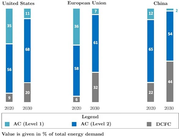
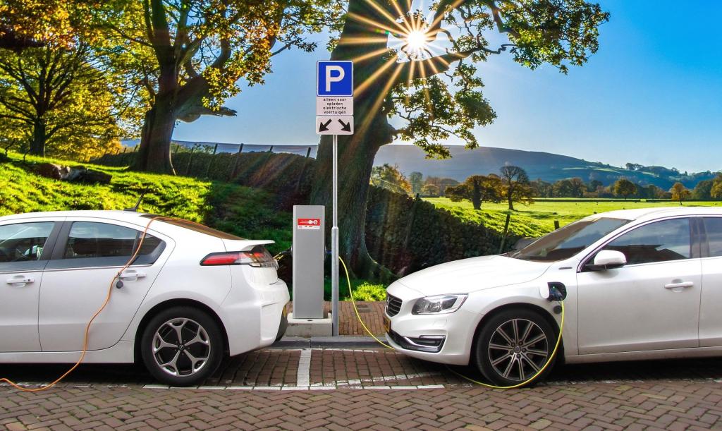
To achieve these results and maintain the current upward trend, electric vehicles must be widely used in the future (Fig.2.). Although they still have a small market share, there is an increasing interest in this type of technology. This is achieved by overcoming their traditional bottleneck, which provides short range, high price (these two are mainly related to the battery) and lack of charging infrastructure, also of quick type [4].

To illustrate the main “deceleration of expansion” of the electric vehicle in the simple comparative analysis of EV and a diesel–powered car, the cost of purchase, annual operating costs, replacement cost of batteries (after 8 years for EV), fuel cost, electricity costs, and the assumed monthly distance covered on the level of 1500 km [5].

As can be seen from the graph (Fig. 1.), electric vehicle is more expensive to use today than traditional drive. However, the important fact is that EV has a much lower increase in costs over time –– it is more stable, of course, after an agreed period, there is a drastic increase in costs caused by the replacement of batteries, but nevertheless, in the longer term, its use looks appealing.

Fig.1. Running costs of an electric vehicle and a car with an internal combustion drive [5]
Fig.2. Car fleet in Poland [6]

The second factor limiting the interest in the electric vehicles is the lack of charging infrastructure. Currently, for the vast majority of EV holders, the charging process takes place at home, by connecting to a household power grid. The average charging time is so long that charging takes place at night and the small range of the battery limits long journeys.

Guided by the above–mentioned factors, the work presents charging methods for electric vehicles, infrastructure, future charging possibilities and the current application of the solution. The battery capacity and discharging tests are shown. One of the most popular cars in the EV sector – the Fiat 500e – was used for the analysis. Investigating the driving dynamics and its length shows the dependence of battery discharge and charging times

The infrastructure of charging electric vehicles

The appearance of electric vehicles permanently in the public space will mean a drastic change in consumer behaviour by offering them a new quality of movement – quiet, dynamic and ecological. However, to make this happen, the previously mentioned development of charging infrastructure for EV is necessary [7].

There is currently a division into three groups of charging stations for EV. The power level at the charging point has a significant effect on the battery charging time of the EV. We currently distinguish:

I –the charger fits inside the car. From the distributor, alternating current is sent from a standard 230V single–phase socket. The converter power to be obtained is limited to 2 KW, which results in charging the battery depending on the capacity from 11 to 14 hours.

II – The charger fits inside the car. The vehicle is loaded with alternating current, one or three–phase. The power can reach up to 20 KW, which means that the charging time is reduced to 2 – 3 hours,

III – In this case, the charger is outside EV. The vehicle’s battery terminals are connected to a special connector located on the vehicle. It requires a DC power supply. The system’s power reaches up to 50 KW. This method allows you to charge up to 80% of the battery capacity in just 15 – 30 minutes, and the battery is fully charged in 1 hour [8].

Fig.3. Annual increase of charging points (forecasts for Poland) [6]

With the development of the market there will be various types of chargers for electric cars. One of them will be ultra–fast charging stations for DC electric cars with 100 kW and 300 kW. Their purpose will vary depending on where they are placed (Fig.3.). On highways, expressways, usually at hotels, restaurants or service areas, stations with high powers will be installed, for direct current, where the most important factor will be time, not the price of the service. In this case, customers will be willing to stop for 30–45 minutes to replace the battery for another 200––300 km [7]. It should be emphasized that even if the stations belong to many charging operators – CPO (Charging Point Operators), they will be associated with consistent settlement systems, enabling each client to use them, e.g. by means of a mobile application or RFID card, to enable moving over long distances in the country and in Europe. The situation was different in cities where cars travel a lot smaller distances, more often they park and can be loaded during overnight stays. The city infrastructure is developed primarily at freestanding stations (available in public or private areas, e.g. in garages of underground housing estates), equipped with slow or medium–speed chargers – between 11 and 22 kW AC.

A completely different concept, in contrast to the charging of contact electric vehicles, is charging wirelessly. For many, free of defects and providing unlimited range when electrified roads. In this type of charging, the most promising solution is the use of energy transfer on the principle of magnetic induction. A system composed of two coils, one in the vehicle of the other at the stopping place, magnetically coupled and forming a transformer with a large air space. The coil located in the transmitter generates a variable electromagnetic field, while in the coil placed in the vehicle, under the influence of this field, a variable electromotive force SEM is created. The energy after conversion in the charger charges the batteries [8]. Such a system is very simple to use and at the same time resistant to external factors [2]. Most often wireless power systems are used to power machines on production belts, however, for electric vehicles, such a system was also developed at the end of the nineties by General Motors.

There is also another way of wireless charging, based on the principle of electromagnetic resonance. The resonance system is mounted in the vehicle. EV charging occurs after the electromagnetic resonance of the transmitter and receiver is synchronized. This method is so much better than during charging there is no need for precise positioning of the system components. A big plus is a more efficient energy transfer. It is possible to transmit power of 3.3 kW at a distance of 20 cm, with losses of only 10%. These systems are lighter and much smaller than induction systems. The magnetic resonance charging method is cheaper, easier to build and safer compared to other wireless methods [8].

The classification and evaluation of wireless charging systems have:

the power of the system that determines the duration of the loading process
the acceptable distance between the surface of the ground and the location of the system in the vehicle,
energy conversion efficiency, determined between the power supply network and the battery terminals
tolerance in positioning the vehicle on the parking spot,
vehicle dimensions and weight.

Another way to charge an EV that is considered but used only in a pilot manner is charging by changing the battery. The process involves replacing a discharged battery with a charged one, and charging takes place outside the vehicle. Battery replacement is to take place in a specially constructed station, which will be fully automated, and the entire process will be supervised and performed by robots [8]. In the future, the entire battery replacement process will take no more than one minute. However, as of today, the price of such a service has not been provided.

A separate aspect connecting directly with the infrastructure for charging electric vehicles will be the settlement of the charging process. The charging price will probably vary depending on the charging time, location and type of charger. This is also a big challenge for legal regulations on this topic.

In the future, science will probably create other ways of loading. Although today we would like the “fuel” that is electric energy to be available in such a way as to ensure driving safety in the context of the distance covered. This change in the way of refuelling will be both a challenge for customers and an opportunity for owners of residential and commercial properties to meet this emerging need. Ultimately, charging stations for EV will become common, democratization will take place in access to them, especially if the business or individual clients invest in their own renewable energy sources [7]

Battery discharge measurements

In addition to charging infrastructure, another issue in the context of the use of electric vehicles is their operation, i.e. energy consumption [9]. In the European Union in the approval tests, the energy consumption of electric vehicles is determined in accordance with the procedure described in UNECE Regulation No. 101. The vehicle is tested on a chassis dynamometer in the NEDC test, this test simulates urban and extra–urban driving [10]. In order to increase the level of information on the properties of electric vehicles, other tests are also performed in running tests, corresponding to different traffic conditions, as well as in traction conditions, during the actual use of the vehicle [11] [12].

To describe the energy and economic properties of electric vehicles, the concepts characterizing energy efficiency and consumption are used.

For electric vehicles without braking energy recovery, the efficiency system is defined as follows:

drive efficiency

.

battery charging efficiency

.

general efficiency

.

where: NT – the power of the electric drive of the car, NR – power resistance, NCH –battery charging power.

For an electric vehicle with braking energy recovery, the efficiency system is defined as follows:

drive efficiency

.

efficiency of braking energy recovery

.

where: NB – braking power of the electric machine, NU – braking energy recovery power.

Road energy consumption is described as a derivative of the energy consumed relative to the distance travelled by the vehicle. For an EV without braking energy recovery, the road energy consumption is:

.

where: s – expensive vehicle, L(T)(s) – work of electric vehicle drive as a function of the road.

For an electric vehicle with braking energy recovery, the road energy consumption is:

.

where: LU(s) – regenerative braking energy as a function of the road [12].

The paper presents the results of an examination of an EV Fiat 500e model in urban conditions. The aim of the study was to assess the road use of energy, the battery power of its linear or non–linear decrease in terms of the number of kilometres travelled and the analysis of battery consumption in different driving dynamics and in the use of other systems existing in the car (such as air conditioning). Below is the technical data table of the car.

Table 1. Data for an electric car Fiat model 500e

.

The Fiat 500e is equipped with a traction drive with a maximum power of 83 kW, making it one of the more dynamic electric vehicles available on the market. Disputes for such a small car is also placed under the seats of a pack of batteries, accumulating 24 kWh of energy. To charge the batteries, Fiat decided to use only a 6,6 kW onboard charger. The car was produced in 2015 in Mexico and imported to Poland from California. At the beginning of the tests, the meter’s mileage was 56335 km. The car roamed the routes in the city in the summer season at ambient temperatures from 22 to 27 oC.

During the tests, the battery level before and after the route and the length of the route itself was checked. The analysis of the data collected during the tests shows that the considerable mileage of the car and hundreds of charging cycles did not negatively affect the battery condition in the car. The battery still retains its initial capacity. The tests were conducted in conditions of normal car use, in standard quiet and dynamic conditions of driving, in traffic jams, with the use of air conditioning and without. The main goal of the research was to see if the battery maintains a linear power drop or in higher battery power ranges the range of the car is greater. For the tests, a car with a considerable mileage was intentionally selected to eliminate the “new battery” syndrome. After analyzing the data, there was no significant deviation in relation to the linear decrease in the range of the car along with the decreasing level of battery charge. The graph below (Fig.4.) presents all 17 measurements showing the number of kilometres driven in relation to the decrease in battery power expressed in percentage points.

Fig.4. Dependency of the route travelled and the level of battery charge drop in% points

For most of the measurements made, the ratio of the battery power drop and kilometres travelled ranged from 0,8 to 1,2. For several measurements, the results did not differ much from this level, the points marked with a square in the graph show a higher value of the power drop per one kilometre travelled. Such measurements belong to exceptionally dynamic routes and for the air conditioning system in operation. With such parameters of driving, faster battery discharge is observed. The point on the graph marked with a triangle shows a short ride in the traffic jam with the air conditioning set to the lowest temperature – for this route, there were about 2,6 points of the power drop per one kilometre travelled.

After the analysis, it was noticed that the length of the route is less important than its dynamics and driving style. For constant speed the power loss will be in a linear and predictable way while driving with a higher load on one battery charge, we will travel a longer route. Nevertheless, the energy saved is not significant enough to be a determinant and determines the driver’s behaviour.

Summary

Most electric vehicle is sold in Norway, France, Germany and the United Kingdom (these four countries account for 72.4% of all new registrations of EV in Europe [5]), almost in all Europe, the number of registered electric cars is growing every year. As the markets show, the development and popularity of electric vehicles is surprisingly growing year by year, but nevertheless most importantly can be recognized as the fact that:

the current development priority for electric vehicles is the development of charging infrastructure,

the decision on the purchase of an EV in addition to the price is decided by the range and the possibility of charging, in most cases only the newly created charging points of electric vehicles are able to influence the decision of the buyers regarding the type of drive,

ensuring the possibility of loading, we eliminate the fears of limited distance that can be overcome,

choosing a car with electric drive on a large scale will affect the ecology and the environment – the elimination of harmful gases and dust will absolutely improve the comfort especially in large urban agglomerations where the traffic volume is the greatest.

Studies of energy consumption by electric vehicles are usually carried out under homologation conditions. In the case of tests carried out, it was tried to reproduce the conditions of normal car use as faithfully as possible, i.e. in the presented work it was shown that:

to reproduce the everyday conditions of car use, the car was introduced into a traffic jam, subjected to smooth and smooth driving and dynamic driving with the use of on–board systems,

research results showed a fairly low sensitivity of energy consumption to the vehicle traffic model,

noticeable increased energy consumption from the battery was noticed while driving in a traffic jam, with the air conditioning system turned on and for dynamic and fast

nevertheless, in all cases the average energy consumption per one kilometre of the route is satisfactory and gives the opportunity and perspective for the spread and popularization of electric vehicles on the roads.

LITERATURA

[1]. U.S. Energy Information Agency. International Energy Outlook 2014; (2014)
[2]. Guziński J., Adamowicz M., Kamiński J., Infrastruktura ładowania pojazdów elektrycznych, Automatyka-Elektryka-Zakłócenia, 1/2014, (2014)
[3]. Zielińska A., Skowron M., Bień A., Infrastruktura fotowoltaiczna do ładowania pojazdów elektrycznych — Photovoltaic infrastructure for charging electric vehicles, XXVIII sympozjum środowiskowe PTZE, ISBN10: 83-88131-99-0., (2018), 370–372
[4]. Nunesn P., Figueiredo R., Brito M. C., The use of parking lots to solar-charge electric vehicles, Renewable and Sustainable Energy Reviews, 66/2016, (2016), 679–693
[5]. http://samochodyelektryczne.org/wyniki_sprzedazy_aut_elektrycznych_w_europie_w_2017r_kraje_i_modele.html for 23.07.2018
[6]. Korolec M., Boleska K., Napędzamy Polską Przyszłość, 19.02.2018.
[7]. https://www.muratorplus.pl/technika/instalacjeelektryczne/stacje-ladowania-samochodow-elektrycznychrodzaje-stacji-ladowania-sposoby-rozliczen-aa-AsuM-ME8B-93W8.html for 01.10.2018
[8]. Zajkowski K., Seroka K., Przegląd możliwych sposobów ładowania akumulatorów w pojazdach z napędem elektrycznym, Autobusy, 7-8/2017, (2017)
[9]. Chłopek Z., Lasocki L., Badania zużycia energii przez samochód elektryczny w warunkach ruchu w mieście, Zeszyty Naukowe Instytutu Pojazdów 1(97)/2014, (2014)
[10]. Raslavičius L., Starevičius M., Keršys A., K. Pilkauskas K., Vilkauskas A., Performance of an all–electric vehicle under UN ECE R101 test conditions: A feasibility study for the city of Kaunas, Lithuania. Energy, 55(15), (2013), 436–448
[11]. Lorf C., Martínez–Botas R.F., Howey D. A., Lytton L., Cussons B., Comparative analysis of the energy
consumption and CO2 emissions of 40 electric, plug–in hybrid electric, hybrid electric and internal combustion engine vehicles. Transportation Research Part D, z. 23, (2013), 12–19
[12]. Wantuch A., Kurgan E., Gas P.: Numerical Analysis on Cathodic Protection of Underground Structures, in 2016 13th Selected Issues of Electrical Engineering and Electronics (WZEE), IEEE Xplore, (2016)
[13]. Chłopek Z., Badanie zużycia energii przez samochód elektryczny,https://depot.ceon.pl/bitstream/handle/123456789/562/POL_2012_3_Badanie_zuzycia_energii_przez_samochod_elektryczny.pdf?sequence=1&isAllowed=y for 01.10.2018


Source & Publisher Item Identifier: PRZEGLĄD ELEKTROTECHNICZNY, ISSN 0033-2097, R. 95 NR 1/2019. doi:10.15199/48.2019.01.38

Solar Power Plant with Distributed System of PV Panels

Published by Mariusz ŚWIDERSKI, Michał GWÓŹDŹ, Poznan University of Technolog


Abstract. In the work the other approach to a photovoltaic system is presented. With regard to an improvement of reliability of a solar system, maintaining and improving system’s efficiency, authors proposed conception of the distributed PV system. This system consists of a set of individual small PV panels, while a single panel is connected to a low power converter, equipped with a pulse transformer. The converters work at a common energy container (battery). Thus, in case of failure of a single converter (or panel) the system is able to work properly with small only decrease of an output power, apart, maintenance of system operation is facilitated. In addition, due to all converters operate independently, individual environmental conditions (e.g. panel’s temperature) can be respected so system’s efficiency can be improved. In the work basics of system operation and selected system’s simulation model findings are presented.

Streszczenie. W pracy przedstawiono inne podejście do struktury systemu fotowoltaicznego. W odniesieniu do poprawy niezawodności działania systemu, obniżenia jego kosztów utrzymania i poprawy wydajności pracy, autorzy zaproponowali koncepcję tzw. rozproszonego systemu ogniw PV. System ten składa się z zestawu niewielkich paneli PV gdzie, pojedynczy panel jest dołączone do przekształtnika energoelektronicznego małej mocy, wyposażonego w transformator impulsowy. Transformator zapewnia mu indywidualną izolację galwaniczną. Konwertery pracują na wspólny zasobnik energii w postaci baterii LiION. Tak więc, w przypadku awarii pojedynczego konwertera (lub panelu), system może działać dalej, przy zmniejszonej mocy wyjściowej. Ułatwiona jest również obsługa (naprawa) systemu. Ponadto, ponieważ konwertery działają niezależnie od siebie, mogą brane być pod uwagę indywidualne warunki środowiskowe dla każdego panelu – na przykład jego temperatura, czy stopień zaciemnienia. W niniejszej pracy przedstawiono podstawy działania systemu i wybrane wyniki badań modelu symulacyjnego pojedynczego panelu. Elektrownia solarna z rozproszonym systemem ogniw fotowoltaicznych

Keywords: big data system, flyback converter, photovoltaic cell, solar system.
Słowa kluczowe: big data system, cela fotowoltaiczna, przetwornica flyback, system solarny.

Introduction

Currently, photovoltaic systems solutions consist of a single PV panel and a single converter or group of PV panels and a single converter. Taking into account mainly the improvement of the reliability of the solar system while, maintaining or even increasing the efficiency of energy conversion, a solution using a distributed system, i.e. separation of the PV on practically single cells (or a few) and coupling it with low power electronics converters is proposed in [1]. This approach requires very sophisticated controlling and refreshing the already known structures of inverters, but also the control algorithms. In addition, there will be considered option to implement in converters modern transistors based on gallium nitride (GaN) material. In this case, it is required to develop a new method of control of power devices in the structure of power converters [2]. The characteristics of GaN transistors let achieve a much higher switching frequency – in relation to Si or even SiC devices. However, at the present stage of the work low loss, ultra fast power MOSFETs are taking into account.

The main goal of the research is to increase the reliability of the system and the resultant efficiency of the entire system, so that it could be achieved the greatest efficiency of converting solar energy into electricity. For this purpose mini converters with a total power equal to the power of a single photovoltaic panel to which, they are connected. Such a solution can increase the reliability of the system, because in the event of failure of one of the DC/DC converters or PV panels, the device can continue to operate with less power, and service of devices can take place at a convenient time, moreover converters operate sequentially with regard to their working conditions e.g. temperature, in order to achieve the operational wear to be uniform. In the studies will be verified the validity of the thesis that converters in distributed system may have a higher conversion efficiency of electricity.

The proposed solar energy conversion system includes an energy container based on LiION cells. This one is common for an entire system and preserves a continuity of energy supply for a consumer e.g. during time of reduced solar radiation. This work presents the initial stage of the project of the solar power system.

Basics of system

The general conception of energy generation system based on distributed PV panels is shown in Fig. 1.

Fig.1. Block diagram of energy generation system based on distributed PV panels

The system consists of the following blocs: set of low voltage photovoltaic panels (PVP) in the number of N , set of low power converters (CNV), where an individual converter is coupled with a single PVP, energy container (EC) – based on LiION cells, power grid side converter (GCN), coupling EC with a power grid, and global control block (GCB), including dedicated big data control algorithm (BDCA). The individual converters are connected to GCB via isolated data-control bus.

The CNV block includes a flyback converter with local controller (LCT). The LCT monitors: PVP’s output voltage ( uPV ), PVP’s output current ( iPV ), and temperature (TPV ) of the panel. On base of these quantities the LCT realizes the Maximum Power Point Tracking (MPPT) algorithm.

In the extended version of the system (Fig. 2) the CNV block contains a larger number (i.e. K) of lower power flyback converters, being connected in parallel. If power transferred by a single flyback converter reaches its nominal capacity, another converter is switched on, etc.. Thank to this they operate in conditions, being close to nominal ones. As a consequence, it is expected, that overall system’s efficiency will grow. Moreover, an order of turning on of another converter is not fixed. This one bases on pseudorandom algorithm. So, the expected system’s lifetime should increase.

Fig.2. Diagram of CNV block in its extended version

The essence of system’s control is to provide a matched power to a load, while maintaining reliability at a high level for the entire structure. The algorithm is characterized by high dynamics of operation, while maintains all principles involved in design of converters for solar systems, e.g. MPPT [3]. Solar radiation falling on photovoltaic panels is disturbed by many factors, e.g. polluted air and, sediments on the panels or even cloud cover. Therefore, the density of luminous flux for particular photovoltaic panel is not uniform. Due to this aspect of the application of the control using MPPT algorithm in a distributed system causes the individual and more effective adjustment to the maximum received power from each photovoltaic panel. In addition, the algorithm receives information about both operation of the converters and state of the loads.

The data used in the analysis is based on Big Data algorithms, to effectively predict the behavior of both the generation side and the load side. The justification for the selection mechanisms of Big Data [4, 5] is dictated by the presence of a large diversity in the collected information, and also to achieve adequately fast prediction of events (i.e. an increasing demand for power by the load or set of loads, the decline in power generation by reducing the light radiation generated by the sun or the temperature increase of photovoltaic cell) in the operation of the entire system, there is a need to collect vast amounts of information – this would include eclectic parameters measured in virtually every component of the system and the load terminals, and ending with the data collected from the environment such as temperature and solar irradiance.

Big Data systems according to the 4V [6] model should meet the following requirements:

volume – have large amounts of data,
velocity – characterized by high variability of data,
variety – consists of a large variety of data,
value – system should collect data of significant values.

In order to meet these requirements, a set of algorithms responsible for the operation of the system was developed. The first of the described algorithms is the algorithm controlling the system startup section – shown in Fig. 3. The system should operate independently. Therefore, the detection of the number of DC / DC converters with which it works is crucial in the start phase. If this process is completed successfully, the system will proceed to database analysis. However, if the system does not detect the connected converters or does not communicate with them, the user will be informed about the system error.

During the boot sequence data analysis is mainly based on counting the number of records in the database. On this basis, the average polling time of system components is determined. In case of slow-changing systems, this limits the size of the database by the reduced frequency of system polling. In other case for processes with significant dynamics, the amount of data will increase accordingly in order to be able to correctly calculate system behavior patterns at a later stage. If the size of the database is not greater than the accepted minimum ( Rmin ) then the system accepts a random (from the range) response frequency, which the system will be able to correct.

Fig.3. System’s startup sequence algorithm

The second described algorithm shown in Fig. 4 is the algorithm responsible for data acquisition.

Fig.4. Data acquisition algorithm

The main task of the algorithm is to collect data and save it to the database. Then, based on the data collected in the database, the average polling time of system components is updated. Next, the demand for system power is determined. If this demand is lower than the power of the whole system then the algorithm can turn off the least effective elements of the system. The reason for low efficiency may be shading, dirt or breakdowns. This algorithm operates in a closed loop and its operating frequency is automatically selected.

The last presented algorithm is the algorithm responsible for deleting records from the database [5]. This one is shown in Fig. 5.

Fig.5. Database cleaning algorithm

In parallel with the control procedure, the system ensures that the database contains only relevant records. Hence, cyclically selected parameters records are read from the database and compared to averaged parameter values. If the average value differs from the analyzed value by the pre-determined degree of accuracy ( e ) – then the record is deleted. If the analyzed value is unique, i.e. it differs significantly from the averaged value, the analyzed record remains in the database.

The next step in the research of the distributed system of converters will be to check the different methods of arranging photovoltaic panel modules, e.g. in the shape of a paraboloid, a sphere section or other hypersurfaces. In the case of a flat arrangement of modules, the energy of reflected radiation is lost. However, in the proposed solution it is possible to reuse part of this energy. Arranging the modules in the shape of a hypersurface additionally contributes to averaging the value of energy received during the day. In comparison to the classic system, the maximum energy consumption is clearly higher than the average and falls at noon. Laying the panels in the shape of a hypersurface additionally eliminates the need for an expensive mechanical system to keep up with the sun (“sun-follower”) [3, 7] or expensive optical elements.

Simulation model studies

At the present project’s development stage simulation studies devoted to the converter in the CNV block (in ORCAD/SPICE environment) were conducted.

The simulation model of this block (in simplified form) is shown in Fig. 6. Basic parameters of the model are as follows:

PV panel output voltage: 2.4÷2.7 V,
PV output current (max): 2.0 A,
energy container voltage (nominal value): 48 V,
switching frequency of MOSFET in CNV block (max): 100 kHz.

Functionality of main blocks in the simulation model is as follows: PVP is PV panel’s model (PV contains three small PV cells connected in series), SW is the power switch model, and CTB is the control block model. The pulse transformer’s model (TX1) was based on a real planar transformer with ferrite core type EEQ30 (N97 material) from TDK. The power switch model was based on modern OptiMOS™ 5 100 V power MOSFET type BSZ146N10LS5 manufactured by INFINEON [8]. Thanks to suitable design of the pulse transformer (both a flat core and multilayer windings) its coupling factor is close to 1 ( k ≅ 0.995). Thus, taking into account, that magnetizing inductance is equal to ~25 µH, the leakage inductance (associated with the primary winding) is equal approximately to 100 nH. As a result, a form of the snubber circuit (R56-C31) can be very simple.

Fig. 6. Block diagram of CNV simulation model
Fig.7. Waveforms of voltages and currents in CNV simulation model, while converter operates in: a) DCM mode, b) CCM mode

In Fig. 7 waveforms of selected voltages and currents in the simulation model are shown. As can be observed, a magnitude of primary current in the DCM is equal to 0.75 A, whereas in the CCM is equal to 1.8 A. A value of power transferred to the energy container was in the range 0.8÷3.0 W – depending on the mode of operation of converter. As it is shown, magnitudes of voltage spikes, in the power switch transient states, are relatively low. In a result the value of energy, dissipated in the snubber circuit, is negligible from point of view of converter efficiency.

Conclusions

The entire study aims to determine the level of reliability of the proposed solution and check how significant is impact of the efficiency of power electronic converters on the overall efficiency of solar energy conversion system. At present stage of system developing the general structure of control algorithms was proposed. With regard to an improvement of reliability of a solar system, maintaining and improving system’s efficiency authors used the distributed PV system consists of a set of individual small PV panels, while a single panel is connected to a low power (micro) converter, equipped with a sophisticated pulse transformer. The converters work at a common energy container (e.g. LiION battery stack). Thus, it is expected, that in case of failure of a single converter (or cell in panel) the system will be able to work properly with small only decrease of an output power, apart, maintenance of system operation is facilitated. Also, findings may open a new way for use of the GaN transistors in systems, where the energy conversion efficiency is crucial, and en energy’s source is limited in power or difficult and expensive to operate.

REFERENCES

[1] Z. Jin, M. Hou, F. Dong, and Y. Li, A new control strategy of dc microgrid with photovoltaic generation and hybrid energy storage, Power and Energy Engineering Conference (APPEEC), (2016) IEEE PES Asia-Pacific, 2016.
[2] Gwóźdź M., Matecki D., Power electronics controlled voltage source based on modified Sigma-Delta modulator, Proceedings of the 2016 IEEE International Power Electronics and Motion Control Conference (PEMC), Bulgaria, Varna, 25-30 September (2016), ISBN: 978-1-5090-1797-3, pp. 186-191. DOI: 10.1109/EPEPEMC.2016.7751995.
[3] Degeratu S., Alboteanu L., Rizescu S., Coman D., Bizdoaca N., and Caramida C., Active solar panel tracking system actuated by shape memory alloy springs, Applied and Theoretical Electricity (ICATE), (2014) International Conference on, ISBN: 978-1-4799-4161-2.
[4] Swartz R.A., Lynch J.P., Zerbst S., Sweetman B., and Rolfes R., Structural monitoring of wind turbines using wireless sensor networks, Smart Structures and Systems 6, 114, (2010).
[5] Najafabadi M. M., Villanustre F., Khoshgoftaar T. M., Seliya N., Wald R., and Muharemagic E., Deep learning applications and challenges in big data analytics, Big Data, vol. 2, no. 1, March (2015).
[6] Erhard R., The case for holistic data integration, East European conference on advances in databases and information systems, Berlin: Springer; (2016).
[7] Zamojski W., Theory and technique of reliability, (in Polish), Wrocław University of Technology, Wrocław, (1976).
[8] Infineon product page: https://www.infineon.com/cms/en/product/power/mosfet/. Accessed: December 2017.


Authors: mgr inż. Mariusz Świderski, E-mail: Mariusz.Swiderski@put.poznan.pl, dr hab. inż. Michał Gwóźdź, Email: Michal.Gwozdz@put.poznan.pl, Politechnika Poznańska, Instytut Elektrotechniki i Elektroniki Przemysłowej, ul. Piotrowo 3A, 60-965 Poznań.


Source & Publisher Item Identifier: PRZEGLĄD ELEKTROTECHNICZNY, ISSN 0033-2097, R. 95 NR 2/2019. doi:10.15199/48.2019.02.11

Trends in Electric Vehicle Fast Charging

Published by Rakesh Kumar, EE Power – Technical Articles: Trends in Electric Vehicle Fast Charging, February 02, 2023.


Ultra-fast charging methodology, ultra-fast charging station architectures, and improved battery technology are some promising trends for fast-charging electric vehicles.

EVs hold the potential for decarbonizing the transportation sector. But the crucial impediment to the adoption of electrified transportation is the charging time taken by an EV. A fuel-based vehicle takes only 15 minutes or less to refuel. Therefore, to encourage the use of EVs, the charging time is expected to match that of fuel-based vehicles.

EV charging. Image used courtesy of Pixabay

Fast charging is key to alleviating range anxiety issues associated with EVs. Various trends are observed in the fast charging of EVs, such as ultra-fast charging, higher battery capacity, and architectures for ultra-fast charging stations.

Ultra-Fast Charging is the Future

Figure 1 shows that the energy demand for EVs is set to go up drastically in the near future. The energy demand is considered in three emerging economies that will boost the adoption of EVs. The illustration in Figure 2 throws light on the importance of fast charging in the coming years. Fast charging is on the roadmap of every emerging economy to boost EV usage. The level 2 and DC fast charging will witness a surge in its share of the total energy demand as time passes.

Figure 1. Total energy demand by EVs. Image used courtesy of IEEE Open Journal of Power Electronics
Figure 2. Energy demand by charging mode of EVs. Image used courtesy of IEEE Open Journal of Power Electronics

The DC fast chargers are rated at 50 kW, marching towards ultra-fast charging. Most drivers prefer to charge the EV battery within 15 minutes which is very challenging from a technological perspective. Some commercially available EV models that capture such fast charging technology are Mini Copper SE, BMW i3, Hyundai Kona, Tesla Model 3, and Tesla Model S. The battery capacity ranges from 25 to 95 kWh, with a range starting from 180 km to 515 km.

Better Battery Technology

As EVs continue to evolve, their battery capacity is expected to increase. The advancement in power electronics technology alone cannot achieve ultra-fast charging. The current battery technology limitations also restrict how fast we can charge an EV. Energy capacity is one of the battery parameters to look out for in long-range EVs. Lithium-ion batteries are the most suitable for EVs of the many existing battery technologies globally. The lithium-ion batteries have a higher power and energy density compared to its counterpart. These features help in removing the EV range anxiety problems of the masses.

The material composition of electrodes used in the lithium battery is a key factor in deciding the energy density of the battery technology. Lithium-ion batteries can be charged in 15 minutes with an energy density of 150 Wh/kg or more with the latest state-of-the-art materials. CATL company has utilized graphite and lithium nickel manganese cobalt oxide (NMC) as an anode and cathode, allowing the battery energy density of 215 Wh/kg. Kokam is another battery manufacturing company with the same anode and cathode composition, offering a battery energy density of 152 Wh/kg. Enevate has utilized Si and NMC as anode/cathode compositions for an energy density of 350 Wh/kg.

Thermal management is another serious issue with battery management. As the energy and power density of the battery increases, it is crucial to look out for proper thermal management practices. Overheating is a fundamental thermal management problem in an electric vehicle. The battery packaging is not designed properly to avoid cooling loss in the battery pack. Such an event leads to events where the battery catches fire, and the whole EV is engulfed in flame. EV battery performance is also affected by cold temperatures. Lithium-ion batteries tend to perform slowly in charging and discharging batteries when placed at very low temperatures. Hence, in such a case, a nominal battery temperature is necessary through mild heating without overheating the battery pack. A third issue prominent in the thermal management of EV batteries is thermal runaway conditions. It is a phenomenon where an increase in temperature aids in further heating up batteries if the temperature is not regulated properly.

Ultra-Fast Charging Station Architectures

The ultra-fast charging station needs to employ its unique architecture to enable fast charging of different EVs connected to it. These stations are most expected along long-distance highways where regular charging is necessary for EVs. Tesla’s fast charging stations consist of nearly 10 to 12 direct current fast chargers, each one bearing a capacity of 150 kW. Therefore, a typical fast charging station has to be rated at 1.5 to 1.8 MW capacity. It is advisable to draw the power from a medium voltage grid for such high power. The low-voltage grid cannot handle such high power, and it might also put an additional burden on the transformers used.

Figure 3 shows a conventional AC distribution network-based ultra-fast charging station. This architecture utilizes multiple AC to DC converters dedicated to each charging point. The AC distribution network is, at present, the most mature architecture, and it is easily viable commercially.

Figure 3.  An AC distribution network-based ultra-fast charging station. Image used courtesy of IEEE Open Journal of Power Electronics

Figure 4 shows the DC distribution network-based ultra-fast charging station. This architecture is currently being researched for its efficiency and commercial viability. This architecture utilizes a simpler architecture with a reduced number of conversion stages. A single AC-to-DC converter is used, after which the DC power is distributed to all the charging points. A promising future ahead for the DC-based network configuration is the usage of Solid State Transformer in the initial conversion stage to replace the combination of medium voltage grid and AC to DC conversion stage. It helps improve the overall system’s efficiency with a battery control mechanism due to the use of power electronics technology.

Figure 4.  A DC distribution network-based ultra-fast charging station. Image used courtesy of IEEE Open Journal of Power Electronics

Figure 5 offers greater insight into the different power electronics converter topologies of an AC distribution network-based ultra-fast charging station. It consists of AC-to-DC and DC-to-DC power conversions. The AC-to-DC conversion is also called the power factor correction stage, the first of the two stages of fast-charging power conversion. Three topologies commonly used for this stage are the Vienna rectifier, conventional 2-level voltage source rectifier, and multi-pulse rectifier. The common features of all these topologies are simplicity in design, higher reliability, and their ability to draw input currents with low harmonics distortion. The second stage is the DC-to-DC conversion stage, where three commonly used topologies are the Half-Bridge LLC, interleaved buck converter, and dual active bridge converter. These topologies can provide galvanic isolation between the EV and grid to enhance the reliability of the whole charging station.

Figure 5. Different power electronics topologies for DC fast charging. Image used courtesy of IEEE Open Journal of Power Electronics

A modular structure of power electronics converters in the DC fast charging is useful in many ways. It helps distribute the voltage and current stress equally among the different modules. Each module can cater to the unique voltage level demand. Therefore, modularity allows for different voltage and power handling capacities within an ultra-fast charging station. As the modules are spaced at a reasonable distance from one another, it allows for proper cooling of each module. In the future, the power handling capacity of an ultra-fast charging station can be increased or decreased by adding or deleting the individual modules.

Key Takeaways of Electric Vehicle Fast Charging

Electrified transportation is witnessing some trends in fast charging. The article has highlighted and briefly explained some important trends. Some of the takeaways of the article are as follows.

Ultra-fast charging is the need of the hour to facilitate charging the EV battery in the least possible time possible.

Battery technology will play a pivotal role where the main challenge is increasing the battery energy and power capacity.

Increasing the battery capacity also needs to address critical thermal management issues. Overheating, cold climatic environments, and thermal runaway conditions are key points in thermal management.

AC and DC distribution-based ultra-fast charging stations are the two architectures that have a high potential to cater to the demands of fast charging. AC-based architecture is mature enough and is the ideal starting point.

However, DC-based architecture is gaining popularity due to the emergence of Solid State Transformers, which can better control and simpler conversion stages.

This post is based on an IEEE Open Journal of Power Electronics research article.


Author: Rakesh Kumar holds a Ph.D. in Electrical Engineering with a specialization in Power Electronics from Vellore Institute of Technology, India. He is a Senior Member of IEEE, Class of 2021, and a member of the IEEE Power Electronics Society (PELS). Rakesh is a committee member of the IEEE PELS Education Steering Committee. He is passionate about writing high-quality technical articles of high interest to readers of the EE Power Community. You can email him at rakesh.a@ieee.org.


Source URL: https://eepower.com/technical-articles/trends-in-electric-vehicle-fast-charging/

Prediction of Electricity Production in Island Operation under the different Wind Generation Modes

Published by Dušan MEDVEĎ1, Zsolt ČONKA1 Marek PAVLIK1, Ján ZBOJOVSKY1,Michal KOLCUN1,Michal IVANČÁK1, Technical University of Košice, Department of Electric Power Engineering, Mäsiarska 74, 04001 Košice, Slovakia (1)


Abstract. This paper deals with the prediction of electricity generation in particular part of the network (island operation) where were considered various regimes of the wind power plant as a one of the power sources. The simulation network was created in Matlab/SimscapePowerSystem environment that consisted of rotating generators (for regulation of power due to fluctuated wind power generation) and wind power plant of variable energy generation and loads. There were considered the following wind power plant regimes: dynamic wind speed and dynamic load; dynamic wind speed and constant load; constant wind speed and dynamic load. From the all regimes were created prediction diagrams which form the day diagram of load.

Streszczenie. Artykuł dotyczy prognozowania produkcji energii elektrycznej w wydzielonej części sieci pracującej wyspowo, gdzie rozważano różne reżimy eksploatacji elektrowni wiatrowej jako jednego ze źródeł mocy. Sieć symulacyjna, opracowana w środowisku Matlab/ SimscapePowerSystem, składała się z wirujących generatorów (do regulacji mocy z uwagi na fluktuacje generacji wiatrowej) i elektrowni wiatrowej o zmiennej generacji energii i mocy. Rozważano następujące reżimy pracy elektrowni wiatrowej: dynamiczną prędkość wiatru i dynamiczne obciążenie; dynamiczna prędkość wiatru i stałe obciążenie; stała prędkość wiatru i dynamiczne obciążenie. Ze wszystkich reżimów powstały diagramy predykcyjne tworzące dobowy przebieg obciążenia. (Prognozowanie produkcji energii elektrycznej w pracy wyspowej dla różnych trybów generacji wiatrowej).

Keywords: wind power plant, off-grid network, flicker –effect.
Słowa kluczowe: elektrownia wiatrowa, praca wyspowa, efekt migotania.

Introduction

This article presents the particular results of the simulation of the impact of various electricity sources on a small off-grid. Diesel generators and wind turbines have been used as power sources. From the point of view of electricity consumption, the effect of disconnection or connection of a large load on the system and the effect of a dynamically changing load is described. Multiple circuits have been simulated to verify some of the network phenomena. The main monitored variables included network frequency, voltage at the point of consumption, and power produced by sources.

To simulate these phenomena, the Simscape Power Systems, which is an extension of Matab Simulink, was used. Based on the simulation analysis, a simple solution was developed to reduce the impact of transient phenomena. Since simulated transient phenomena of a short nature, i.e. they take a short time, the designed simulations simulate the time interval within 1000 seconds, which is about 17 minutes. A short time interval has also been chosen because the results that are written in matrices have some accuracy and can be processed with current common computing techniques.

Description of the network model of components in the environment of Simscape Power Systems

In the Simscape Power Systems, several electrical machines are implemented. Many of these electrical machines can work in two states – as electricity generators or as motors, that is, as electric consumer appliances [1, 2]. Model of the synchronous machine with expressed poles was used. The synchronous generator is controlled by a hydraulic turbine combined with the PID control system and excited by the AC4A excitation system. The principal scheme of the G1 generator with a control and exciter system and generating output from the generator can be seen in Fig. 1.

Output of the synchronous generator is a three-phase voltage at the terminals of the machine A, B and C and the measurement output marked with the letter “m”. The measurement output includes a vector with measured signals: stator currents, stator voltages, rotor angle deviation, rotor speed, electromagnetic torque, output active power P, output reactive power Q, and so on. These signals receive feedback from the generator that is input to the exciter winding input and the hydraulic turbine with the control. The label data of the simulated generator are shown in Table 1.

Fig.1. Principal scheme of the G1 generator connection

Table 1. Data of the simulated generator.

.

In Fig. 2 is a model of a hydraulic turbine with PID control. This model has 5 inputs and 2 outputs. Inputs include reference speed, instantaneous mechanical speed, speed deviation, reference power and instantaneous power output. The output is the mechanical power Pm, which is also the input for the synchronous generator. In the mentioned model was set the reference speed ωef = 1 pu, and the inputs of the immediate mechanical velocity ωe and the velocity variation dω were connected. This regulation ensures the regulation of the synchronous generator at the nominal frequency fn = 50 Hz. Inputs of the reference mechanical power Pref and instantaneous power Pe0 are not connected. The circuit is set so that it does not take any feedback (or feedback from the gate output). It has been achieved that the turbine power was controlled only by rotor speed [7].

Fig.2. Hydraulic turbine diagram with PID control
Wind turbine

The wind turbine block with power-out transmission to the grid is considerably easier than a block of PV field. The wind turbine input is the wind speed reported in m·s–1 and a Trip connector. The wind speed for this model was retrieved from a text file. Trip connector serves to simulate the turbine protection system. Its input may be a logical zero or one. If at input port is logical zero, the wind turbine is in operation and when at input is logical one, the turbine is disconnected. The wind turbine can have several protections. First of all, it is a wind turbine disconnection when there is slow/fast wind, but also overcurrent protection, undervoltage protection, overvoltage protection, or protection, acting in the unbalanced current or voltage.

The wind turbine output is a measuring port that contains the voltage and current at turbine terminals A, B and C, turbine output P and Q, turbine rotor speed, mechanical torque, and so on. The wind turbine used in this article includes, in addition to the turbine, also an asynchronous engine that generates the electrical energy. In Fig 3 is shown the characteristic output of the designed turbine at different wind speeds.

Fig.3. Characteristic turbine power at different wind speeds

Since during the simulation the disconnection of the wind turbine caused a mathematical error, the block “Check static range” was added to the scheme. This block stops the simulation if a wind speed is read at a speed that is not in the work range, and Matlab shows error message. The wind turbine operating range is in ranges from 4.5 m·s–1 to 12.5 m·s–1. The basic wind speed for the model turbine was set to 9 m·s–1.

Definition of Loads

Simscape Power Systems offers several types of loads. In this article, three-phase serial RLC load and three-phase dynamic load were used. For both loads, the combined nominal voltage and nominal frequency of the network were entered.

Fig.4. Wind turbine block with power delivery to the system

For a static three-phase load, PQ power was entered, which may be the same or specific for each load in all three phases. A static three-phase load contains also a voltage and current measurement that is optional [3, 4, 6].

For dynamic three-phase load, the PQ power was entered at the beginning of the simulation. The PQ power of a dynamic load can be controlled by an internal control that controls the amount of dynamic load based on the positive sequence voltage component. If external control of power source is used, performance can be read from a file, and controlled by an external handling. The dynamic load contains also a measuring terminal „m“, the output of which is a vector with a positive-sequence voltage component, an active power P and a reactive power Q [5, 10].

Fig.5. Loads in Simscape Power Systems (3-phase series RLC and 3-phase dynamic load)

The loads were read using a Matlab script. In Fig 6, a proposed load block for the supply point A is shown. On the left, the load A1 and line A2 are shown, which are connected to the system via a three-phase circuit breaker and a power line simulated by the impedance Ra and La. Line A2 consists of a purely ohmical load, because the dynamic load line A1 cannot be connected in series with the inductive element of the three-phase line, which is the supply point connected to the system. On the right, the reading of block of line load A1 is displayed. If init_const = 1, the load, i.e. line A1 is set according to the vector from a text document. If init_const = 0, the load is set to the constant value, which is set in the text document for time t = 0. Current and voltage measurements were performed on bus-bar A. During the simulations, four consumption points A, B, C and D were considered. Each of these consumption points represents a part of the network. In some simulations, only static three-phase consumption points were used that were disconnected by a three-phase switch.

Measurement in Simscape Power Systems

In the simulations, electrical quantities were measured at selected locations in the network. Phase currents and voltages were measured using three-phase V-I measuring blocks, which were placed before loads and before the generators, resp. other sources. The measured output is the sinusoidal voltage/current depending on the time that has to be converted to the effective value (for comparison purposes). The scheme for measuring of the particular variables at the output of the G1 generator is shown in Fig. 7. The RMS current and voltage values for the L1 phase and the active and reactive power in the L1 phase were calculated from the measured currents and voltages.

Fig.6. Designed load block with control
Fig.7. Scheme for control and measuring of monitored quantities
Model of a steady-state off-grid network
Fig.8. The steady-state model diagram

In the off-grid steady-state model, the main aim was to point out that if no changes were made to the scheme and the correct initialization conditions were set, the network’s frequency did not change and was 50 Hz. The phase voltage in phase L1 is equal to the portion of the line-to-line voltage and the square root of 3. If in a system were also considered losses on the line, the resulting voltage values were less than the expected 230 V. In the system were considered large losses on lines, so the phase voltages at the terminals were lower, namely: Ua_A = 220.5 V, Ua_B = 221 V, Ua_C = 223.1 V, and Ua_D = 227 V. The demand current depends on the size of the load being connected at the consumption point (load). The active and reactive PQ load was unchanged in the circuit.

Table 2. Consumptions for simulation of steady-state off-grid network

.
Model of off-grid network with dynamic load

In this part of the simulation there was modified model of loads. Instead of the loads modeled by the constant value, dynamic loads were used that were controlled by external input. Dynamic load operation is described in the previous chapter definitions of loads During these simulations, two generators with a nominal power of 250 kVA and four loads A, B, C and D were used in which the phase voltage and current in phase L1 and power value in L1 were measured.

Fig.9. Network frequency response to output power

In Fig. 9, the consumed power is indicated by dynamic loads. Self-consumptions (2 x 12.5 kW) and parasitic loads to dynamic loads (3 x 9.5 kW + 4.75 kW), which are purely resistive, have to be added to the total output power. These parasitic loads are in the system because dynamic loads and synchronous generators cannot be in series with an inductive element of three-phase power lines. Those are described by the RL parameters listed in Table 3.

Table 3. Resistance and inductance of power lines in simulations with dynamic load

.

By a continual decreasing, respectively by increasing of the power consumption there was observed, that the regulators of the synchronous generators respond to these changes, and there is a decrease, respectively increase in output power produced by synchronous generators, but the frequency is not regulated to the nominal value of fn = 50 Hz. Thus, the frequency of the network will be short-lived at a different value near the nominal frequency due to the rate of decrease/increase of the consumed power. This can also be seen in Fig. 9, from 478 seconds to 595 seconds, the network’s frequency was around 50.2 Hz. From 900 s to 1000 s the network frequency was stable at values between 49.93 and 49.95 Hz.

Off-grid model with a wind turbine that operates at a dynamic wind speed

Wind simulation was used to simulate the wind-flow circuit as it is illustrated in Fig. 10. The wind loaded from the text file has a value of 9 m·s–1 at time t = 0, which is the nominal wind for the wind turbine used. Subsequently the wind varies around this value. Wind reaches a maximum value of 12 m·s–1. The wind turbine operates with winds ranging from 4.5 m·s–1 to 12.5 m·s–1.

Since the simulated wind turbine has no stabilizing mechanism, the supplied turbine power also varies around the nominal value. This was reflected negatively on network frequency and voltage. Since the simulated off-grid network is small in size, voltage fluctuations have been registered in all four A, B, C and D loads. Frequency of the grid and voltage at the wind turbine terminals are shown in Fig. 10. Referring to Fig 10 it can be seen that even with small wind changes, the frequency has risen above 51 Hz, or falls below 49 Hz. Voltage at wind turbine terminals is fluctuating. In case of a sudden change of wind, the voltage exceeds 250 V, respectively drops to 190 V. Since the voltage fluctuations are relatively strong, a digital flickermeter has been connected to load points A, B, C and D and to the wind turbine connection point.

Fig.10. Simulated wind parameters
Flicker-effect measurement in network with a wind turbine

In the previous section there was a description of offgrid operation with a wind turbine with dynamic wind. In order to determine the flicker effect in the aforementioned network, a digital flickermeter was added at points A, B, C and D to find a short-term flicker rate that is calculated at simulation time of 5 to 605 s, representing a ten-minute time period. In Table 4 is the measured short-term rate of flicker and averaged percentiles. The smallest rate of flicker shortterm perceptive was simulated with a constant wind velocity of 9 m·s–1 and a dynamic load. On the other side, the highest short-term flicker rate was simulated with dynamic wind speed and dynamic load. The short-term flicker rate was in accordance with standard STN EN 50160.

The Fig 11 shows the measured instantaneous level of the flicker effect at the load point C for dynamic load simulation (Fig. 9) and the dynamic wind simulation (Fig. 10). From Fig. 11, it is apparent that the blink effect was occurred in the case of dynamic load simulation at a time when the load was connected or disconnected in the network. It was observed for example, at time t1 = 100 s when a load of 30 kVA was disconnected at the load point B or at time t2 = 400 s when a load of 20 kVA was connected at the load point C or at time t3 = 800 s when the load of 20 kVA was disconnected from load point C. In the case when the dynamic wind acts on the wind turbine (see Fig. 10), the measured instantaneous level of flicker effect will appear as a stochastic noise.

Fig.11. Measured instantaneous level of flicker effect

The Table 4 shows the short-term flicker rate response for the load points A, B, C and D and for the point on the wind turbine terminals. The particularity of these results is that in each simulated scheme, at the load point A, the highest degree of short-term flicker is measured. This is due to the fact that the point A is powered by a line whose resistance and reactance is much larger than the lines connecting the other points (see Table 3). The voltage at point A in these simulations was stabilized at U = 189.6 V (in real conditions, such a low voltage would be a problem for the operation of many devices).

Table 4. Flicker effect in the simulated network

.

In order to reduce the influence of power line on the measured flicker effect, the simulations were repeated except that the line joining the load point A was simulated by resistance Rc = 0.0134 Ω and inductance Lc = 23.7 µH connecting the load point C. The results are given in Fig. 12.

Fig.12. Voltage in simulated scheme for point A

In Fig. 12 is the voltage characteristics at the load point A in the case where was considered constant wind of 9 m·s– 1 during the whole simulation and the dynamic load as described in section B. For the case 1 there was considered the original power line whose resistance was Ra = 0.2010 Ω and inductance La = 355.5 µH. In case 2, a point A was connected by a line with parameters Ra = 0.0134 Ω and La = 23.7 μH. From Fig. 12, it is clear that in case 1 there is a greater voltage fluctuation at the terminals at the load point A as in case 2. For example, during the disconnection of the 20 kVA load from the load point C, there was observed (in case 1) at the load point A the short-term voltage drop from Uf = 194.3 V to Uf = 149.5 V, which is a drop of ΔU = 44.8 V. In case 2, there was drop from Uf = 225.7 V to Uf = 199.4 V, which is drop of ΔU = 26.3 V. As there is less voltage fluctuation in transient phenomena, the resulting flicker effect will be less. In test example 2, the value of the Short Term Perceptibility (Pst) of flicker effect in point A was Pst = 0.335491 (the original value, in case A was Pst = 0.523317).

Conclusion

This article presented the particular results of off-grid network simulations with consideration of renewable resources (wind turbine) and without considering renewable energy sources. The simulated off-grid network consisted of two diesel generators with a nominal output of 250 kW and with loads A, B, C and D, representing 4 load points representing 4 off-grid sites. In the case of a load disconnection or connection, the generators are able to regulate the system so that the power output is equal to the power delivered. The regulation of diesel generators has ensured the control of the hydraulic turbine.

The problem of off-grid systems with a wind turbine (WT) is that the power output from the WT cannot be regulated. The WT produces electricity according to current climatic conditions. Therefore, in the case of rapid climate change, there is a rapid change in the output of the WT. For example, with decreased wind speed, a sudden drop in the electricity produced from the WT may occur. By adding a wind turbine into an off-grid, an increased flicker effect was observed. In addition to voltage fluctuations in the network, the network frequency also varies. Large frequency fluctuations can have a negative impact on diesel generators. Flicker effect occurs when disconnecting or connecting loads, resources, and off-grid networks. In both cases, it is necessary to consider how to remove the unfavorable phenomenon of blinking. For this reason, it is necessary to have good data for prediction of electricity production in island operation under the different wind generation modes.

Acknowledgement This work was supported by the Ministry of Education, Science, Research and Sport of the Slovak Republic and the Slovak Academy of Sciences under the contract No. VEGA 1/0372/18.

REFERENCES

[1] M. Špes, Ľ. Beňa, M. Kosterec, M. Márton, Determining the current capacity of transmission lines based on ambient conditions, In: Journal of Energy Technology. Vol. 10, no. 2 (2017), p. 61-69. ISSN 1855-5748
[2] R. Cimbala, L. Kruželák, S. Bucko, J. Kurimský, M. Kosterec, Influence of Electromagnetic Interference on Time-Domain Spectroscopy of Magnetic Nanofluids, In: EPE 2016. Danvers: IEEE, (2016), p. 279 – 282. ISBN 978-1-5090-0907-7
[3] D. Medveď, O. Hirka, Investigation of Electromagnetic Fields in Residential Areas. In: Acta Electrotechnica et Informatica. Vol.17, No. 3 (2017), p. 48-52. ISSN 1335-8243
[4] T. Košický, Ľ. Beňa, Optimizing deployment of battery storage systems, In: Current Problems of Maintenance of Electrical Equipment and Management. Košice: TU, 2014 p. 131-141. ISBN 978-80-553-1818-9
[5] V. Volokhin, I. Diahovchenko, V. Kurochkina, M. Kanálik, The influence of nonsinusoidal supply voltage on the amount of power consumption and electricity meter readings, In: Energetika. Vol. 63, no. 1 (2017), p. 1-7. ISSN 0235-7208
[6] Z. Čonka, M. Kolcun: Impact of TCSC on the Transient Stability In: Acta Electrotechnica et Informatica. Vol. 13, no. 2 (2013), p.50-54. – ISSN 1335-8243
[7] MathWorks, Model hydraulic turbine and proportional-integralderivative, https://www.mathworks.com/help/physmod/sps/powersys/ref/hydraulicturbineandgovernor.html
[8] MathWorks, Three-Level Bridge, https://www.mathworks.com/help/physmod/sps/powersys/ref/threelevel bridge.html
[9] MathWorks, Av. Model of a 100-kW Grid-Connected PV Array, https://www.mathworks.com/help/physmod/sps/examples/average-model-of-a-100-kw-grid-connected-pv-array.html
[10] MathWorks, Implement three-phase dynamic load with active power and reactive power as function of voltage or controlled from external input, https://www.mathworks.com/help/physmod/sps/powersys/ ref/threephasedynamicload.html
[11] Ž. Eleschová, A. Beláň, B. Cintula, B. Bendík, Smart grids analysis – View of the transmission systems voltage stability, In EPE 2018. Brno: University of Technology, 2018, p. 37-42. ISBN 978-1-5386-4612-0
[12] D. Kaprál, P. Braciník, M. Roch, M. Höger, Optimization of distribution network operation based on data from smart metering systems, Electrical Engineering, Vol. 99, Issue 4, Springer, New York, USA, 2017, December, pp: 1417-1428, ISSN 0948-7921


Authors: Ing. Dušan Medveď, PhD. Technical University of Košice, Department of Electric Power Engineering, Mäsiarska 74, 04001 Košice, Slovakia E-mail: dusan.medved@tuke.sk; Ing. Zsolt Čonka, PhD. Technical University of Košice, Department of Electric Power Engineering, Mäsiarska 74, 04001 Košice, Slovakia E-mail: zsolt.conka@tuke.sk; Ing. Marek Pavlík, PhD. Technical University of Košice, Department of Electric Power Engineering, Mäsiarska 74, 04001 Košice, Slovakia E-mail: marek.pavlik@tuke.sk; Ing. Ján Zbojovský, PhD. Technical University of Košice, Department of Electric Power Engineering, Mäsiarska 74, 04001 Košice, Slovakia E-mail: jan.zbojovsky@tuke.sk; Dr.h.c. prof. Ing. Michal Kolcun, PhD. Technical University of Košice, Department of Electric Power Engineering, Mäsiarska 74, 04001 Košice, Slovakia E-mail: michal.kolcun@tuke.sk; Ing. Michal Ivančák, Technical University of Košice, Department of Electric Power Engineering, Mäsiarska 74, 04001 Košice, Slovakia E-mail: michal.ivancak@tuke.sk


Source & Publisher Item Identifier: PRZEGLĄD ELEKTROTECHNICZNY, ISSN 0033-2097, R. 95 NR 7/2019. doi:10.15199/48.2019.07.31

Overvoltage Induced in Overhead Power Lines by nearby Lightning Stroke

Published by Grzegorz MASŁOWSKI, Robert ZIEMBA, Tomasz KOSSOWSKI,
Rzeszow University of Technology


Abstract. The results of simulations of overvoltages induced in the overhead transmission line, caused by nearby lightning stroke are presented. Calculations were made using the LIOV module implemented in the EMTP-RV program. The influence of the distance of the lightning channel from the line to the overvoltages has been investigated. The results for the various lightning currents in the lightning channel have been compared.

Streszczenie. Przedstawiono wyniki symulacji przepięć indukowanych w linii napowietrznej od pobliskich wyładowań atmosferycznych. Obliczenia wykonano przy użyciu modułu LIOV zaimplementowanego w programie EMTP-RV. Zbadano wpływ odległości kanału pioruna od linii oraz wpływ kształtu prądu piorunowego na kształt i wartości szczytowe indukowanych przepięć. (Przepięcia w liniach napowietrznych wywołane pobliskim wyładowaniem atmosferycznym).

Keywords: lightning protection, lightning induced overvoltages, overhead power line.
Słowa kluczowe: ochrona odgromowa, indukowane przepięcia piorunowe, napowietrzna linia energetyczna.

Introduction

Lightning-induced overvoltages are transient overvoltages on overhead power lines caused by indirect lightning events, i.e. lightning strikes hitting the ground or objects in the vicinity of the lines. In accordance with lightning protection standards IEC 62305 [1-3], the impact of nearby lightning strikes shall be taken into account in the design of the Lightning Protection System (LPS). Although the effects of nearby lightning strikes are smaller than direct impacts, the range of impact is much greater. They cause overvoltage in the indoor installations and in the lines coming into the building.

Computer code LIOV (Lightning Induced Overvoltages) [4-6] was implemented as the special module in EMTP-RV software. Now LIOV module allows for the calculation of lightning-induced voltages along a multiconductor overhead line as a function of:

– lightning current waveshape (peak value, front steepness, and duration), stroke location and return stroke velocity;
– line geometry (height, length, number and position of conductors) and line terminations;
– ground resistivity and relative permittivity.

The geometry for the calculation of LEMP (Lightning Electromagnetic Pulse) and its coupling with an overhead line, implemented in LIOV module is showed in Fig. 1.

Fig. 1. Geometry for the calculation of Lightning Electromagnetic Pulse (LEMP) and its coupling with an overhead line, implemented in LIOV code.

LIOV code adopts an engineering return stroke model and the lightning channel is assumed as a straight vertical antenna [7]. An engineering return stroke model is a formula that describes the spatial and temporal distribution of the return stroke current along the lightning channel, as a function of the current waveshape at the base of the channel and one or two additional parameters. This model with the straight and perpendicular lightning channel was simulated in [8-10] with the MTLL and the MTLE return stroke models in frequency domain.

In the present version of LIOV-EMTP module only the Transmission Line (TL) return stroke model is adopted [11, 12].

Modelling and simulation of lightning induced overvoltages

The most commonly adopted return-stroke models to calculate lightning-induced voltages are [10]: the Modified Transmission Line Linear (MTLL) model; the Modified Transmission Line Exponential (MTLE) model; and the Transmission Line (TL) model. In the MTLL model the current wave propagates without distortion but its peak value decays linearly with height.

In the MTLE model the current wave propagates similarly but the current peak value decays exponentially with height.

In the TL model, it is assumed that the current wave at the base channel propagates up the lightning channel without distortion and without attenuation, at a constant speed v. The return stroke current in the lightning channel at height z is:

.

where: 1(t) is the Heaviside function equal to 1 for tz/v and zero otherwise; v is the upward propagating return stroke velocity; i0(t) is the current at the base of the channel.

The return stroke velocity is expected to be between 100 and 200 m/μs [13]. The channel base current waveform can be represented by means of Heidler function, which is a function of the lightning current for analysis purposes in IEC 62305-1 standard, specified by equation:

.

In (2) I is the peak current, k is the correction factor for the peak current, τ1 is the front time constant and τ2 is the tail time constant.

According to IEC 62305-1 [1], the current shapes of the first positive impulse 10/350 µs, the first negative impulse 1/200 µs and the subsequent negative impulses 0.25/100 µs, defined by Heidler function, were taken for calculation. The peak values for the first lightning protection level (LPL) were chosen (respectively 200 kA, 100 kA and 50 kA). Comparison of waveshape of the lightning current components is shown in Fig. 2.

Fig.2. Waveforms of the lightingThe channel base current (2) can be set in the “liov options” device as shown in Fig. 3, assuming peak value I02 equal zero. current components.
Fig.3. Definition of current waveform in LIOV option module.

In lightning protection standard [2] there are defined the collection areas of flashes directly to line (Al) and to ground near line (AL). This collection areas are taking into account for calculation of the risks of lightning losses. The width of these areas are different in two subsequent editions of IEC 62305-2 standard. The width of collection area of flashes into the line was increased from WI = 30 m to WI = 40 m and the width of the collection area of indirect lightning flashes was increased from WI = 1000 m to WI = 4000 m. As we can see, in the case of indirect discharges, the collection area has been increased four times. This increase of the collection area can be of importance in assessing the risk of the lightning damage in the design of the LPS.

The example of a system that can be simulated with LIOV-EMTP module is shown in Fig. 4. This case study was simulated by using the circuit shown in Fig. 5. The overhead three-wire transmission line of 1000 m in length and 10 m in height was taken to the simulations. Position of the lightning channel is xs = 500 m and ys (distance of the lightning channel from power line is variable: ys1 = 100 m, ys2 = 500 m, ys3 = 2000 m).

The geometrical data of the conductors of the overhead line are represented in Fig.6, where the subscripts of H, D and d refer to the pins corresponding to the line ends.

Fig. 4. Scheme of simulated system.
Fig.5. Analysed circuit in EMTP-RV software.
Fig.6. Definition of conductor geometry in transmission line.

The ends of the transmission line are terminated by “line match” components containing connected to ground characteristic impedances of the line.

Results of the simulation

In Fig. 7 and Fig. 8 are shown the induced overvoltages at the ends of transmission lines, for different lightning current impulses and for different soil parameters. In Fig. 7 are shown results of simulations for case study with lossy ground (soil resistivity: ρ = 100 Ωm). Strike distance ys is variable: 100 m, 500 m and 2000 m. Simulations has been conducted for the first positive impulse 10/350 μs with peak value 200 kA; the first negative impulse 1/200 μs with peak value 100 kA; and for the subsequent negative impulse 0.25/100 μs with peak value I = 50 kA. In Fig. 8 are shown results of simulations for case study with lossless ground, and for soil with resistivity ρ = 100 Ωm and ρ = 500 Ωm. Strike distance ys = 500 m. Simulations has been conducted for the first positive impulse 10/350 μs with peak value I = 200 kA; the first negative impulse 1/200 μs with peak value I = 100 kA; and for the subsequent negative impulses 0.25/100 μs with peak value I = 50 kA.

.

Fig. 7. Comparison of the induced overvoltages for case study with lossy ground (soil resistivity: ρ = 100 Ωm). Strike distance ys is variable: 100 m, 500 m and 2000 m: a) the first positive impulse 10/350 μs, peak value 200 kA; b) the first negative impulse 1/200 μs, peak value 150 kA; c) the subsequent negative impulses 0.25/100 μs, peak value 100 kA.

.

Fig. 8. Comparison of the induced overvoltages for case study with lossless ground and for soil resistivity ρ = 100 Ωm and ρ = 500 Ωm. Strike distans ys = 500 m. a) the first positive impulse 10/350 μs, peak value 200 kA; b) the first negative impulse 1/200 μs, peak value 100 kA; c) the subsequent negative impulses 0.25/100 μs, peak value 50 kA.

To compare voltage distribution along the line in Fig. 9 were shown overvoltages in the middle (xs = 500 m) and at the end of the line (xs = 0 m) for different distance of the lightning channel from the line. Simulation was for the first positive impulse 10/350 μs with amplitude 200 kA.

.

Fig. 9. Comparison of the induced overvoltages in the middle and at the end of the line for first lightning stroke 10/350 200 kA, for different distance of the lightning channel from the line: a) ys = 100 m, b) ys = 500 m, c) ys = 2000 m

Conclusions

The paper presents results of the computer simulations of the overvoltages induced in the transmission line by nearby lightning stroke. Influence of the striking distance, soil resistivity and shape of the lightning current were investigated. As shown in Fig. 7 maximum values of induced overvoltages strongly depend on the distance of the lightning channel from the line. Results in Fig. 8 shows that soil resistivity does not have a significant impact on maximum values and shapes of induced overvoltages within the considered distances. As shown in Fig. 9, the peak values of the induced voltages at the centre of the line relative to the overvoltages on the ends of the line depend on the distance of the lightning channel from the line.

REFERENCES

[1] IEC 62305-1:2010 Protection against lightning – Part 1: General principles.
[2] IEC 62305-2:2010 Protection against lightning – Part 2: Risk management.
[3] NFPA 780 Standard for the Installation of Lightning Protection Systems. 2014.
[4] C. A. Nucci and F. Rachidi, “Interaction of electromagnetic fields with electrical networks generated by lightning,” in The Lightning Flash: Physical and Engineering Aspects, V. Cooray, Ed. IEE – Power and Energy Series 34, 2003, pp. 425–478.
[5] F. Napolitano, A. Borghetti, C. A. Nucci, M. Paolone, F. Rachidi, and J. Mahserejian, “An advanced interface between the LIOV code and the EMTP-RV,” presented at the 29th Int. Conf. Lightning Protection (ICLP), Uppsala, Sweden, 2008
[6] M. Paolone, F. Rachidi, A. Borghetti, C. A. Nucci, M. Rubinstein, V. A. Rakov, and M. A. Uman, “Lightning
electromagnetic field coupling to overhead lines: theory, numerical simulations, and experimental validation”, IEEE Trans. Electromagn. Compat., vol. 51, no. 3, pp. 532–547, 2009
[7] Masłowski G., Rakov V.A.: New Insights Into Lightning Return-Stroke Models with Specified Longitudinal Current Distribution. IEEE Trans. Electromagn. Compat., Vol. 51, No. 3, August 2009, 471–478
[8] Masłowski G. Ziemba R.: Calculation of lightning-induced voltages inside the structure using engineering return-stroke models. Proc. 28th International Conference on Lightning Protection, Kanazawa, Japan, 2006, 1132-1137
[9] Masłowski G., Ziemba R.: Modelowanie przepięć atmosferycznych w liniach elektroenergetycznych z uwzględnieniem kanału pioruna. Przegląd Elektrotechniczny, 3/2007, 153–156.
[10] Masłowski G.: Współczesne trendy w modelowaniu wyładowań atmosferycznych – teoria i zastosowania, Przegląd Elektrotechniczny (Electrical Review), R. 86 NR 11a/2010, 308–312
[11] M. A. Uman and D. K. Mclain, “Magnetic field of lightning return stroke,” J. Geophys. Res., vol. 74, no.28, pp. 6899–6910, 1969.
[12] F. Napolitano, “An analytical formulation of the electromagnetic field generated by lightning return strokes,” IEEE Trans. Electromagn. Compat., vol. 53, no. 1, pp. 108–113, 2011.
[13] V. A. Rakov and M. A. Uman, Lightning: Physics and Effects. Cambridge, 2003.


Authors dr hab. inż. Grzegorz Masłowski, Politechnika Rzeszowska, Wydział Elektrotechniki i Podstaw Informatyki, ul. Powstańców Warszawy 12, 35-959 Rzeszów, e-mail: maslowski@prz.edu.pl; dr inż. Robert Ziemba, Politechnika Rzeszowska, Wydział Elektrotechniki i Podstaw Informatyki, ul. Powstańców Warszawy 12, 35-959 Rzeszów, e-mail: maslowski@prz.edu.pl; mgr inż. Tomasz Kossowski, Politechnika Rzeszowska, Wydział Elektrotechniki i Podstaw Informatyki, ul. Powstańców Warszawy 12, 35-959 Rzeszów, e-mail: t.kossowski@prz.edu.pl;.


Source & Publisher Item Identifier: PRZEGLĄD ELEKTROTECHNICZNY, ISSN 0033-2097, R. 94 NR 2/2018. doi:10.15199/48.2018.02.10

Noise and Vibration Analysis of a Distribution Transformer

Published by Dániel MARCSA, eCon Engineering Kft., Hungary


Abstract. Transformer noise is a significant contribution to unwanted ambient noise, especially in the vicinity of the electrical transmission facility. It is therefore very important to get to know the mechanism of noise generation of the distribution transformer. As outcomes of this work, a finite element based multiphysics model is presented which provides a convenient and efficient toolchain for simulating the transformer sound emission mechanism. Finally, the operation of modelling chain is presented on a 200kVA distribution transformer simulation.

Streszczenie. Hałas transformatora ma znaczący wpływ na niepożądany hałas otoczenia, zwłaszcza w pobliżu instalacji przesyłowej prądu elektrycznego. Z tego powodu ważnym jest poznanie mechanizmu generowania szumu transformatora rozdzielczego. Jako wynik tej pracy przedstawiono model transformatora rozdzielczego 200 kVA oparty na analizie elementów skończonych, który zapewnia wygodny i wydajny zestaw narzędzi do symulacji mechanizmu emisji dźwięku z analizowanego urządzenia. (Analiza hałasu i wibracji transformatora rozdzielczego).

Keywords: Noise and vibration, finite element analysis, coupled simulation, distribution transformer, ANSYS.
Słowa kluczowe: hałas i wibracje, analiza elementów skończonych, symulacja sprzężona, transformator dystrybucyjny, ANSYS.

Introduction

Distribution transformers are one of the most critical components for electrical energy transportation and distribution. The vibration and noise of these electric machines increasingly interested designers and manufacturers. It is therefore critical that manufacturers are able to accurately identify the acoustic characteristics of a transformer before production commences. However, the various physical phenomena are strongly related in the transformers, as illustrated in Fig. 1, so only the multiphysics or coupled numerical simulation can be useful to get knowledge about these effects. Further, safety regulations require that the noise level is kept within a certain range.

The study of noise and vibration in transformers began in the 1930s, mainly by transformer manufacturers [1]. These works are focused on mainly the measurement of transformer noise. In recent years, thanks to the computer capabilities and software, more and more attention has been paid to the numerical simulation of these unwanted effects. However, most of these works are separated the strongly coupled sources or effects of noise and vibration. The noise mainly originates from the magnetostrictive effect of the steel sheet [2], [3] and the shape of the core [4]. The electromagnetic force produced in the windings also important as electromagnetic noise source [5]. The clamping stress and natural frequencies of core and tank also have some effect on vibration [6]. These effects result in deformation of the tank [7], [8], which cause disturbing audible sound. When using coupled or multiphysics simulation, important effects are neglected or analysed only a special load case. Most of the time, the permeability of the transformer core is isotropic [5], [9] or analysed the shortcircuit state of transformer [5], [10]. But a coupled simulation workflow with the whole noise generation process at nominal operation has not been studied.

This work focuses on distribution transformer coupled simulation with the help of the finite element method (FEM) [10], [11]. The aim of this paper is to develop a numerical methodology that accurately predicts the vibration and acoustic characteristic of a distribution transformer under normal operation condition. The modelling procedure is based on the chaining of three analysis methods, the electromagnetic, the mechanical and the acoustic simulations as you can see in Figure 1. The weak or series coupling was used for the connection because in this case completely identical geometry is not needed, finite element mesh and solver options are independent for each analysis.

Fig.1. The process of noise generation by the transformer.

The workflow of the transformer simulation was established using ANSYS Workbench environment. The auxiliary noise sources are not taken into account.

Transformer Coupled Simulation

The geometry of the 200kVA distribution transformer with the sectioned tank is shown in Fig 2a. The transformer core is composed of oriented silicon steel sheets, and the anisotropy of silicon steel sheets should be considered. The B-H curve and magnetostrictive curve of steel sheet in rolling and transverse direction are shown in Fig 3. The key parameters of the transformer are summarized in Table 1.

Table 1. Main technical parameters of the analysed oil-type transformer.

.
Fig.2. CAD model of the distribution transformer (upper) and magnetic flux density vectors in the laminated core (lower).
Fig.3. Magnetisation curves (left) and magnetostriction curves (right) of steel sheet in rolling and transverse direction.

The simulation chain starts with time-dependent nonlinear electromagnetic simulation. The external circuit of excitation and load is directly coupled to the finite element model. The geometry (the active part of the transformer) of the problem is discretized into 273823 tetrahedron elements. The numerical solution of these equations is based on ungauged T, Φ – Φ – formulation [11], [12],

.

where [σ] and [μ] is the conductivity and permeability tensor, T0 is the impressed current vector potential, T is the current vector potential, and HP is the additional field component due to core loss.

The main task of this step is to calculate the Maxwell force and the Lorentz force in the core and windings, respectively. In addition, the different power losses (stranded, eddy current, hysteresis) in the core and the winding can also be determined in this step. The visualization of the magnetic flux density vectors in the core can be seen in Fig. 2b.

The next step is mechanical simulation in the frequency domain. However, resonance in the transformers may be induced when the multiples of excitation frequency are sufficiently close to the natural frequency [6], therefore it should be carried out the modal analysis. The main origin of vibration is the magnetostrictive strain, so the most critical frequency is 100 Hz. The modal analysis results are shown in Fig. 4, where it can be seen that both of them one frequency cannot avoid the 100 Hz.

Fig.4. Simulated results of the natural frequency. The active part vibration at 104.4 Hz (upper) and the tank vibration at 98.8 Hz (lower) natural frequency.

Using the results of the electromagnetic simulation (magnetostriction, Lorentz force) and the natural frequencies from the modal analysis the mechanical displacement is evaluated by harmonic analysis. The solved generalized equation of motion is given as [4]

.

where Mu is the structural mass matrix, Cu is the viscous damping matrix, Ku is the stiffness matrix, ü , , u is the nodal acceleration, nodal velocity and nodal displacement vector, respectively. fe is the spectrum of force from the electromagnetic simulation as load force.

The basic procedure to pass the electromagnetic results from the time domain to the frequency domain mechanical simulation is the Fourier transform [10] of results. The vibration from the core due to magnetostriction contains a 100Hz component (twice the frequency of power source frequency) and harmonics, while the vibration from the winding has mainly a pure 100 Hz tone if the current in the winding themselves are free of harmonics [13].

Figure 5 shows the total deformation of the active parts of the transformer at 100 Hz. The deformation of core and clamp can be seen in Fig 5a and the deformation of the primary and secondary winding in Fig 5b. The maximal deformation at the core is in the upper yoke, where the displacement is greater than 3.5 μm. The maximum of displacement in the windings is right one (Phase C). The maximum deformation of this winding is 3.1 μm.

Finally, using the harmonics displacement, we determine the resulting pressure level of acoustic waves propagation through the insulation oil, the tank and the surrounding air. The nodal velocities of active part from the harmonic analysis have been interpolated and mapped to the acoustic mesh of oil. Fig. 6 illustrates the velocity vectors on the oil inner surface. The numerical prediction of sound radiation has required the oscillation of the transformer tank. Therefore, it is necessary the coupling of (3) and the Navier-Stokes equation of fluid momentum and the flow continuity equation,

.
Fig.5. The deformation of the active part. The core and clamp deformation (upper) and the deformation of winding (lower).
Fig.6. The nodal velocity vectors mapped to the acoustic body surrounding the transformer tank.
Fig.7. The x-, y- and z-component of acceleration on the surface of the middle limb of core.
Fig.8. The x-, y- and z-component of acceleration on top of the transformer tank.

where ρ0 is the mean fluid density, Mq is the fluid mass matrix, Cq is the fluid damping matrix, Kq is the fluid stiffness matrix, fq and fu is the load force and Cfs is the fluid-structure coupling term. The pressure is p = = jωq.

Results and Discussion

The main sources of vibration are the electromagnetic origin, so the accuracy of the electromagnetic model is important. The loss has been used to validate the model. The calculated total loss is 2076 W, which corresponds to the value specified in the datasheet (see in Table I). The main reason for the difference is that there is no information on the load used for the measurement, and an average distribution network as load used in the finite element simulation.

Fig. 7 and 8 show the results of mechanical harmonic analysis at two specific points on the transformer. These figures show the spectrum of x-, y- and z-component of the acceleration. As the modal analysis has shown, one of the resonance frequencies of the active part and the tank is close to twice the excitation frequency. This is also supported by Fig. 7 and 8, because one of the peak values of the acceleration spectrum is at 100 Hz. The tank top has another peak in the spectrum at 150 Hz. Based on this information, the sound pressure level is analysed at 100 Hz. Fig. 9 and 10 summarize the simulation results from the acoustic field simulation. These figures show the sound pressure level at 2 m from the tank wall. 0 degrees and – 180 degrees indicate the centre of the shorter side of the transformer. Reference line shows the 53 dB, which is the noise level of this transformer based on datasheet. These results also support that the accuracy of the result obtained by the numerical simulation is acceptable. As shown in the figures, the sound pressure reaches 60 dB in the 680 mm case. When using A-weighting [13], the sound pressure level increases as shown in Fig. 10. Based on the results, it can be stated that the analysed transformer meets the requirements, but its noise level can be reduced by proper design.

Fig.9. Sound pressure level [dB] around the transformer at 340 mm and 680 mm height and 2000 mm distance from tank wall.
Fig.10. Sound pressure level [dB] and its A-weighted version around the transformer at 680 mm height and 2000 mm distance from tank wall.
Conclusions

This paper analyzes the performance of noise and vibration in the distribution transformer considering the anisotropy and magnetostriction influence of silicon steel sheet. A three-dimensional finite element method based multiphysics workflow in the electromagnetic – mechanical – acoustic field is established using sequential coupling of ANSYS software. The operation of the 3-D finite element workflow is analyzed via a 200 kVA distribution transformer problem. It shows that the simulation is in a reasonable agreement with the transformer datasheet value, verifying the validity of the presented coupled simulation. The presented simulation workflow seems to be appropriate for simulating transformer noise and vibration or it may be helpful to develop new transformer diagnosing method.

The future plan is to further develop the presented workflow to take into account the structure-borne transmission of sound waves through the transformer mountings and auxiliary noise sources, e.g. oil pump. In addition, the speed up and simplification of simulation workflow also an ongoing task.

The research for this paper was financially supported by the EU and the Hungarian Government from the project “Intensification of the activities of HU-MATHS-IN – Hungarian Service Network of Mathematics for Industry and Innovation” under grant number EFOP-3.6.2-16-2017- 00015.

REFERENCES

[1] IEEE Commi t te Repor t , Bibliography on Transformer Noise, IEEE Transactions on Power Apparatus and Systems, PAS-87 (1968), 372-387
[2] Zhang P., Li L., Cheng Z., Tian C., Han Y., Study on Vibration of Iron Core of Transformer and Reactor Based on Maxwell Stress and Anisotropic Magnetostriction, IEEE Transactions on Magnetics, 55 (2019), No. 2, 9400205
[3] Chen D., Hou B., Feng Z., Bai B., Study of Magnetostrictive Influence of Electrical Sheet Steel Under
Different DC Biases, IEEE Transactions on Magnetics, 55 (2019), No. 2, 2001305
[4] Shuai P., B iela J., Impact of Core Shape and Material on the Acoustic Noise Emission of Medium Frequency, Medium Voltage Transformers, 17th European Conference on Power Electronics and Applications (EPE’15 ECCE-Europe), Geneva (2015), 1-11
[5] Duan X., Zhao T., Liu J., Zhang L., Zou L., Analysis of Winding Vibration Characteristics of Power Transformers Based on the Finite Element Method, Energies, 11 (2018), No. 9, 2404
[6] Hsu C.-H., Lee S.-L., Lin C.C., Liu C.-S., Chang S.-Y.,
Hsieh M.-F., Huanf Y.-M., Fu C.-M., Reduction of Vibration and Sound-Level for a Single-Phase Power Transformer with Large Capacity, IEEE Transactions on Magnetics, 51 (2015), No. 11, 8403204
[7] Vieira N., Antunes P.J., Martins C., Dias G.R., Coelho A.T., Vibro-Acoustic Analysis of a Distribution Power
Transformer Using the Finite Element Method, CWIEME 2008 – Coil Winding, Insulations & Electrical Manufacturing, Berlin (2008), 1-10
[8] Shengchang J., Lingyu Z., Yanming L., Study on Transformer Tank Vibration Characteristics in the Field and Its Application, Przegląd Elektrotechniczny, 2011 (2011), No. 2, 205-211
[9] Kubiak W., Wi tc zak P., Vibration Analysis of Small Power Transformer, COMPEL – The International Journal for Computation and Mathematics in Electrical and Electronic Engineering, 29 (2010), No. 4, 1116-1124
[10] Kaltenbacher M., Numerical Simulation of Mechatronic Sensors and Actuators, Springer-Verlag, Berlin, 2007
[11] Kuczmann M., I ványi A., The Finite Element Method in Magnetics, Akadémiai Kiadó, Budapest, 2008
[12] Lin D., Zhou P., Chen Q.M., Lambert N., Cendes Z.J., The Effects of Steel Lamination Core Losses on 3D Transient Magnetic Fields, IEEE Transactions on Magnetics, 46 (2010), No. 8, 3539-3542
[13] Tímár P.L., Fazekas A., Kiss J., Miklós A., Yang S.J., Noise and Vibration of Electrical Machines, Akadémiai Kiadó, Budapest, 1989


Author: dr. Dániel Marcsa, Ph.D., eCon Engineering Kft., Kondorosi u. 3, Budapest, H-1116, Hungary, E-mail: daniel.marcsa@econengineering.com.


Source & Publisher Item Identifier: PRZEGLĄD ELEKTROTECHNICZNY, ISSN 0033-2097, R. 95 NR 12/2019. doi:10.15199/48.2019.12.38

The Impact of EVs on the Electric Grid

Published by Harsha Korde, EE Power – News: The Impact of EVs on the Electric Grid, May 14, 2022


With gas prices rising, electric vehicles are becoming more popular, but transportation decarbonization remains a major issue.

With gasoline prices rising and the effects of climate change increasingly acute, transportation electrification is gaining steam in countries throughout the world. The benefits of a transition toward electric vehicles (EVs), and away from the compressed natural gas (CNG) fueling those with traditional internal combustion engines (ICEs), are many: reduced carbon emissions, less noise pollution, improved air quality and enhanced energy efficiency, among others.

Planning for Electric Vehicles

That said, transportation decarbonization remains a significant issue in many countries whose power systems are dominated by fossil fuels. Though the switch to EVs will have direct repercussions for power grids, power system planning to assess EV impacts is practically nonexistent, leaving systems managers with an incomplete view of the technical and economic impact of EV integration.

Electric vehicles (EVs) charging. Image used courtesy of Pixabay

As EVs increasingly supplant ICE-based vehicles, changing demands in power utilization will play an ever more critical role. These demands can have a range of impacts on the power network, such as an increase in the number of short circuit currents, and can lead to voltage level violations, in addition to affecting electrical equipment such as transformers.

Chief among concerns is the load placed on the grid by EV charging. In a world where millions of EVs saturate the road, at any moment the grid could face an influx of stress from simultaneous, mass charging. That uncertainty makes it significantly harder for operators to balance grid supply and demand in real-time. At scale, an increased load on the distribution network impacts its power quality, and if EV batteries are charged without an analysis of their impact on the distribution network, it may directly result in an increase of energy unserved by the power system or the need for additional peak load capacity.

The Distribution Level

To address this issue at the distribution level, different load management schemes should be implemented alongside existing distribution network policy, including time-varying tariffs and incentives for different charging behaviors. But even with these, the frequent connecting and disconnecting of high-current EV batteries pose its own challenges to the efficient operation of the electrical power system.

The net electrical energy utilized by EVs in a specific area is termed a “charging load curve” of EVs for that area. To analyze the impact of EV penetration on the electrical grid, the predictions provided by this load curve are essential. In impact evaluation, an EV load curve analysis can aid in evaluating various fundamental parameters of the electrical power distribution system, such as overloading, the impact on a domestic transformer, power loss in the system, the stability of the grid, fluctuations in voltage, power quality, and stress on distribution cables or conductors, and so on. Developing a full picture of those impacts as a result of EV charging is vital, as the prime objective here is to construct charging infrastructure integrated with the grid well enough to ensure smooth operation and maintenance of the distribution network.

When EV charging is carried out in a three-phase power system, it results in voltage imbalance, since those chargers are single-phase. Because of the increased load, the introduction of power electronics to the charging process also results in the injection of harmonics. This can be the cause of rising transformer temperatures at the distribution feeder, leading to wear of the transformer bushings. Harmonic distortion can as well affect the interruption capability of circuit breakers. These issues can be res

V2G Technology

EV smart charging involves vehicle-to-grid (V2G) integration technology, allowing car batteries to give back to the power grid. In this way, the high-capacity batteries powering EVs can function as backup storage for the electrical grid. This type of setup utilizes bidirectional charging stations, where the power flow is directional based on the electricity demand at any given time. The extra energy can be used to power houses, buildings or anything connected to the power grid.

V2G integration technology has numerous benefits, such as improving the efficiency of power distribution. In a scenario where most EVs are charged simultaneously during peak hours, or at any time when energy demand is high, the system could easily be overloaded. With V2G technology, though, power companies can expand their capacity to meet these peaks; the bidirectional energy flow of V2G offers the most efficient model of power distribution. An additional benefit of this technology is the increase it could promote in renewable energy utilization, such as solar and wind, which will play an important role in sustaining the economy. Though these sources may be inconsistent, an efficient power grid can capture energy through them whenever needed and store it for distribution. Still, whenever there is a surge in energy capture, perhaps thanks to high winds, grid-level system storage has the potential to be maxed out. And that’s where EV batteries and V2G technology come in—with millions of EVs on hand ready to charge, there is additional room to capture and utilize this extra energy. When taken together, the above benefits also lead to another: cost stability. The more strain on the system, the higher the costs. Given that, the improved balance between energy supply and demand will naturally lead to less volatile pricing.

An Uphill Battle?

All that said, there is still much work to be done in fully realizing bidirectional V2G integration technology. Today, most electric vehicles and charging stations are unidirectional, and converting them to the bidirectional form will require significant investment. There is also no standardized cadre of rules and regulations governing V2G integration technology, but rather a hodgepodge of electrical standards applied across varying jurisdictions, making the implementation of such technology difficult. In the face of these challenges, there is a lack of clear incentives for household and business customers to convert to smart charging systems. As such, in moving forward with an effective transition to true V2G integration technology infrastructure, a top priority is to address these obstacles.


Source URL: https://eepower.com/news/the-impact-of-evs-on-the-electric-grid/

Reliability of Open Public Electric Vehicle Direct Current Fast Chargers

Published David Rempel1, Carleen Cullen1,2, Mary Matteson Bryan1, Gustavo Vianna Cezar3,
1Department of Bioengineering, University of California, Berkeley, CA, USA
2Cool the Earth, Kentfield, CA, USA
3SLAC National Accelerator Laboratory, GISMo Group, CA, USA


Abstract. In order to achieve a rapid transition to electric vehicle driving, a highly reliable and easy to use charging infrastructure is critical to building confidence as consumers shift from using familiar gas vehicles to unfamiliar electric vehicles (EV). This study evaluated the functionality of the charging system for 657 EVSE (electric vehicle service equipment) CCS connectors (combined charging system) on all 181 open, public DCFC (direct current fast chargers) charging stations in the Greater Bay Area. An EVSE was evaluated as functional if it charged an EV for 2 minutes or was charging an EV at the time the station was evaluated. Overall, 72.5% of the 657 EVSEs were functional. The cable was too short to reach the EV inlet for 4.9% of the EVSEs. Causes of 22.7% of EVSEs that were non-functioning were unresponsive or unavailable screens, payment system failures, charge initiation failures, network failures, or broken connectors. A random evaluation of 10% of the EVSEs, approximately 8 days after the first evaluation, demonstrated no overall change in functionality. This level of functionality appears to conflict with the 95 to 98% uptime reported by the EV service providers (EVSPs) who operate the EV charging stations. The findings suggest a need for shared, precise definitions of and calculations for reliability, uptime, downtime, and excluded time, as applied to open public DCFCs, with verification by third-party evaluation.

Keywords: electric vehicle charging infrastructure, performance, renewable energy, zero emission vehicles

Background

Reliable, functional, open, public Direct Current Fast Charge (DCFC) electric vehicle (EV) charging stations are critical as countries rapidly transition to EVs. A recent survey of EV drivers in California (N=1290) reported mixed experience with existing EV chargers (CARB, 2022a). They reported experiencing broken plugs (9%), unexpected shut off during charging (6%), charging station not functioning (22%), payment problems (18%), and the need to contact customer service via cell phone (53%). This experience appears to contradict a simultaneous survey of the EV service providers (EVSPs) who reported 95 to 98 percent uptime of their public chargers. An accurate assessment of the reliability, functionality, and uptime of the existing public EV chargers is needed to provide guidance for the successful buildout of the EV charging infrastructure.

Open EV charging stations are those open to all EVs (NREL, 2022). Closed systems, such as Tesla Superchargers, will not accommodate all EVs. Public charging stations are those that are open to the public 24 hours per day 7 days per week (AAI, 2022; NESCAUM, 2019). Examples of non-public charging stations are those in paid parking lots or those limited to customer and employee use. Open, public DCFC charging stations are designed to charge different models of EVs and, therefore, have multiple connector types, such as CCS (Combined Charging System; SAE, 2018), CHAdeMO, and Tesla connectors. Charging stations have one or more kiosks (also called posts), with each kiosk situated adjacent to one or two parking spaces. A kiosk may have one or more EVSEs (Electric Vehicle Supply Equipment) or ports (OCPI, 2020). An EVSE or port provides power to charge only one vehicle at a time even though it may have multiple cables with the same or different connector type (Figure 1). The EVSE provides information on charging and controls the delivery of electricity to the cable (DOE AFDC, 2022). Each kiosk typically includes a payment system that collects payment information from credit cards, debit cards, membership cards or smartphone applications; the transaction may be by tap, insert, swipe, or near field detection depending on the payment method. Another method of payment is Plug and Charge where the only action required is to plug in the EV and the EV is automatically identified and linked to a previously established payment method (ISO, 15118).

Figure 1. A model of an EV DCFC charging station with 2 kiosks or posts, 3 EVSE charge ports, and 4 connectors. Kiosks may have multiple connectors of the same or different types (e.g, CCS, CHAdeMO). [from DOE AFDC, 2022]

The National Renewable Energy Laboratory (NREL) Alternative Fuels Data Center (AFDC) maintains a national database/map of public EVSEs. The database includes charging station location and number of EVSEs (ports) and connection types at each station (NREL, 2022). The data is updated on a periodic basis by EV service providers (EVSPs); some states require updates at least monthly (CARB, 2022b). In addition, commercial smartphone, tablet, and desktop apps, such as PlugShare, provide EV users with information on the location of EV charging stations, the name of the EVSP, the number and types of connectors, the maximum power delivered, and other information.

There are different methods of measuring reliability of an electrical system, but essentially, it is the degree to which the performance of the system results in electricity being delivered to the customer in the amount desired (ORNL, 2004). The reliability of an EVSE, that is, the functional state, can be considered from the perspective of the EVSP or the EV driver. The EVSP may detect the state of an EVSE through its communication network, or as calls to a service number by EV drivers, as a measure of reliability. From the EV driver perspective, a reliable EVSE is one that charges the EV, for the expected duration, after using an appropriate payment method, at the expected rate (i.e., kW). The upper bound on charge rate is influenced by many factors including the EV’s state of charge, the maximum rate allowed by the EV, and the charging station nominal rate. The Alliance for Automotive Innovation (2022) defines a reliability standard as one specifying a minimum uptime requirement. States have different minimum uptime requirements for EVSEs that are paid for with public funds. For the Northeast States (NESCAUM, 2019) “Each connector on each public DC fast charging station pedestal shall be operational at least 99 percent of the time based on a 24 hour 7-day week (i.e., no more than 1.7 hours of cumulative downtime in a 7-day period).” For California, “The equipment must be operational at least 97 percent of the standard operating hours of the charging facility for a period of 5 years” (CEC, 2021).

However, the use of uptime as the reliability metric is controversial since there is no standard definition nor is there a standard calculation methodology. Given the complexity of the EVSE ecosystem and technology stack, from hardware to software, ensuring a high uptime and assigning “uptime ownership” of each EVSE may be difficult and may require standardization across different jurisdictions.

The EVSE ecosystem is composed of different stakeholders. For example, when an EVSE is installed, it is connected to the local utility electrical infrastructure that delivers power to EVSE. The EVSE is installed by a certified installer, operated by the charge point operator (CPO) and located at a site where it may be owned and managed by a site host or the EVSP. The EVSE is connected to an internet service provider (ISP) network and a payment system. Finally, the EVSEs may be serviced by an EV servicing company.

Depending on the jurisdiction, the overall responsibility for keeping the EVSE functioning, can be either with the local electric utility, the installer, the site host, the CPO, or the servicing company. These stakeholders may be independent or may be integrated, i.e., installer can also be the CPO, etc. These stakeholders will likely have different levels of visibility over the status of the system. For example, the site host might have information about the electrical infrastructure and outages and physical damage to kiosks but not information about the functional status of each kiosk, whereas the CPO may have continuous EVSE status information. This partial visibility of the EVSE operation poses a challenge in maintaining a high uptime from the EV driver perspective. Moreover, since these stations are in public locations, events such as road blockage due to construction, theft, or vandalism can occur, which are beyond the immediate control of the CPO. Therefore, the complex nature of the ecosystem and the lack of a clear definition and metrics describing EVSE uptime may interfere with stakeholders’ accountability.

For the purposes of this study, a functional EVSE is one that can charge for a minimum of 2 minutes, using an appropriate payment method, without the need to make a service call. An EVSE includes all the system components within a kiosk that are necessary for a successful charge, including the port, screen, network communication, payment system, power source, software, cable, and connector. If a kiosk has more than one cable with a CCS connector, the functionality of each connector is evaluated and reported as a separate EVSE.

The purpose of this study was to systematically evaluate whether open, public DCFC EV chargers with CCS connectors were functional in the 9 counties of the Greater Bay Area. California has the greatest density of public open DCFC chargers in the US (NREL, 2022) and within California the density is high in the Greater Bay Area.

Methods

All open, public DCFC EV charging stations with EVSEs with CCS connectors in the 9 counties of the Greater Bay Area were identified using the NREL NFDC database and the PlugShare.com website. Stations with CCS connectors with a charge rate >= 50kW were identified. The 9 counties were Alameda, Contra Costa, Marin, Napa, San Mateo, Santa Clara, San Francisco, Solano, and Sonoma. Non-open EV charging stations, e.g., Tesla, as well as non-public EV charging stations, e.g., stations in paid parking lots, private workplaces, or business sites with restricted access hours, were excluded.

The identified EV charging stations were visited by a driver with an EV with a CCS charge inlet. Each EVSE at the station was tested by plugging the CCS connector into the EV and attempting to initiate and sustain a charge for 2 minutes. If the charge was successful, the EVSE was classified as functional. The unique kiosk and CCS connector number or name were recorded. If the parking space was occupied by another EV and the EV was charging, the EVSE was classified as functional. If the parking space was occupied by a non-EV or by an EV and not charging, it was classified as not tested. If none of payment methods tested worked, or the EVSE was not functioning, or did not initiate or sustain a charge, the EVSE was classified as nonfunctional. If the cable was too short to reach the EV charge inlet, the EVSE was classified as a design failure.

The payment methods tested included 2 different functioning credit cards and the vendor mobile app or membership card. Payment methods were tested in the following order, credit card 1 insert, credit card 1 swipe, credit card 2 insert, credit card 2 swipe, then mobile app or membership card, until one of the payment methods was accepted. Each method, i.e, a swipe, was attempted twice before moving to the next payment method. The credit cards used for testing were Mastercard, Visa, and Amex. If any of the payment methods worked and led to a 2 minute charge, the EVSE was classified as functional. The EV drivers were instructed not to call the service number if the EVSE did not work; a functioning EVSE should not require a call to a service number.

Twenty volunteer EV drivers assisted in the testing of the EV charging stations. Only EVs with CCS charge inlets were used. The vehicles used for testing were the Chevy Bolt, Kia Niro, Hyundai Kona, Ford Mustang Mach E, and Porsche Taycan. The EV battery charge level was less than full at the time of testing. The volunteers were trained on the study methods and assigned EV charge stations to test. The survey was completed using a Qualtrics survey on a mobile device while the driver was at the charging station.

A random sample of 10% of the stations was tested at two points in time, approximately 1 week apart, to determine whether the functional state of the EVSEs changed over time.

Results

A total of 181 open public DCFC EV charging stations and 678 EVSEs with CCS connectors were identified in the 9 counties of the Greater Bay Area and visited between February 12, 2022 and March 7, 2022. Of these 678 EVSEs, in 21 instances, the adjacent parking space was occupied by a non-EV (7) or an EV that was not charging (14); therefore, these 21 EVSEs were excluded from the evaluation. The remaining 657 EVSEs that were evaluated are listed by EVSP in Table 1.

Table 1. Evaluated open public DCFC EV charging stations and EVSEs by EV Service Provider

.

1 An EVSE includes all the system components in a kiosk necessary to deliver a charge to a single connector.

Reliability of EVSEs

The functional states of the 657 EVSEs are summarized in Table 2. 72.5% of the EVSEs were functioning at the time of testing; 57.8% were tested and charged for 2 minutes and 15.4% were occupied by an EV that was charging. 22.7% of the EVSEs were not functioning. System electrical failures, e.g., screen blank or non-responsive, text on screen of “charger unavailable” or “connection error”; payment system failure; or charge initiation failure, were the most common causes of failure. A charge initiation failure occurred if the charge did not start after the payment was accepted or the charge started but was interrupted before 2 minutes of charging was completed. A payment system failure was recorded only after all payment methods were tested, each twice, and all failed. A broken connector, e.g., cracked or with bent pins, was recorded for 0.9% of EVSEs.

The cord was too short to reach the EV inlet for 4.9% (N=32) of EVSEs tested. This design failure was recorded at a ChargePoint station (1), EVgo stations (4), and Electrify America stations (27). The EVs tested were driven into the parking space either forward or backward during testing to position the EV inlet as close as possible to the charging kiosk. The EVs used, when it was recorded that the cord was too short, were all Chevy Bolts.

Table 2. Functional states of 657 CCS DCFC EVSEs.

.

1 Charger error, unavailable, under maintenance, etc.
2 Connection, network, communication error, etc.
3 12 of these were evaluated with 2 credit cards but not an app or membership card
4 Short session failure
5 At 3 EVSEs the space was too small to safely back into

Three EVSPs, ChargePoint, Electrify America, and EVgo accounted for 97.3% (639 of 657) of the EVSEs evaluated. The functional states of the EVSEs for the 3 EVSPs are summarized in Table 3. It should be noted that most of the Electrify America kiosks each had 2 CCS connectors that were each tested and reported as independent EVSEs. However, the 2 CCS connectors could not be used simultaneously. If each of these kiosks were considered as a single EVSE, with functionality determined if either just one or both connectors provided a successful charge, the percent of functional EVSEs for Electrify America would have increased from 73.9 to 77.1%.

Table 3. Functional State of EVSEs by the Top 3 EV Service Providers

.

Payment Methods For the 375 EVSEs that charged for 2 minutes, the payment methods that worked are summarized in Table 4. The payment methods were tested in the order presented in Table 4. For example, 50.4% of the successful charges occurred after just the first credit card was inserted. However, 24.5% of the successful charges required an app or membership card for payment, i.e., attempts to pay with 2 credit cards were not successful.

Table 4. Payment method that worked, in the order tested, for the 375 EVSEs that charged for 2 minutes.

.

Testing EV Charging Stations at Two Points in Time

Nineteen (19) randomly selected stations (88 EVSEs) were tested by 2 different EV drivers to determine if their functional state changed over time. The mean time between samplings was 8.0 days (SD=4.9). Eight of the EVSEs could not be compared between the time points because during one of the samplings the EVSE was occupied by a non-EV, an EV that was not charging, or the cord was too short. Of the remaining 80 EVSEs, 48 remained in a functional state, 14 remained in a non-functional state, and 18 (22.5%) changed state from functional to non-functional or a non-functional to functional (5 of these occurred with the same EV model). For the 14 EVSEs that remained in a non-functional state, the cause of failure was the same at both sampling times for 13 of them. The overall functional status changed little between the sampling times, i.e., 72.5% were functional at time 1 and 70.0% were functional at time 2.

Discussion

Of the 657 open public DCFC CCS EVSEs evaluated in this study, 72.5% were functional at the time of testing while 27.5% were either not functional or the cable was too short to reach the EV inlet. The most common cause of a nonfunctional EVSE was an electrical systems failure which included an unresponsive or unavailable screen, a payment system failure, a charge initiation failure, a connection failure, or a broken connector.

This is the first study we are aware of that systematically evaluated the functional state of open public EV chargers. The findings corroborate recent non-systematic surveys of EV owners. In a survey of 1290 EV owners, 34% reported that charging station operability issues were a barrier to using public charging stations (CARB, 2022a). In survey of 5500 EV owners, 25% of those who use public DCFCs reported a major difficulty with chargers being nonfunctional or broken (Plug In America, 2022). In the same survey, only 4% of Tesla owners reported a major difficulty with the Tesla closed DCFC system.

In the Greater Bay Area, 3 EVSPs, ChargePoint, Electrify America, and EVgo accounted for 97.3% of the 657 open public DCFC EVSEs evaluated. There were important functional and design differences between the stations installed by these EVSPs. ChargePoint had the highest percent of non-functional CCS EVSEs at 36.4% followed by EVgo (25.5%) and Electrify America (19.0%). The most critical design flaw was that 7.1% of the Electrify America cables were too short to reach the Chevy Bolt charger inlet, a problem that may be experienced by other EVs with the power inlet on the side of the vehicle. The cable length problem could be addressed with an industry standard on minimal cord length based on the kiosk location relative to the parking space.

The term reliability, when referencing an electrical system, typically refers to the percent of time, over a given time period, that the system is fully operational and able to deliver power at the intended level. This percent is also referred to as the uptime. For public EV charging stations, the definition from the Northeast States, is “the percent of time that a charging station must be functioning properly and available for use by EV drivers” and “Each connector on each public DC fast charging station pedestal shall be operational at least 99 percent of the time based on a 24 hour 7-day week (i.e., no more than 1.7 hours of cumulative downtime in a 7-day period)” (NESCAUM, 2019). New York, California, and the Federal Highways Administration require a minimum uptime of 97% (NYSERDA, 2021; CEC, 2021; FHWA, 2022).

The findings of this study suggest that the currently installed DCFC stations do not meet the 97 to 99% minimum uptime required by public funding agencies. The findings also appear to contradict the 95 to 98% national uptime levels reported by EVSPs (CARB, 2022a, p11). EVSPs do not report the details of how they define and calculate uptime. The EV charging infrastructure would greatly benefit from more data transparency and transparency on methodologies used by each EVSP in calculating uptime. For example, EVSPs could share data on the different subcomponent failure rates and whether the failure was localized, i.e., only affecting one EVSE due to a component failure, or systemic, i.e., affecting multiple EVSEs due to a communication or software problem. Such a reporting mechanism would benefit the entire industry by establishing an ongoing mechanism to identify the weak links in the ecosystem and developing a coordinated approach to addressing them.

While there are state reporting requirements for uptime; there are no precise state, national, or industry consensus definitions of nor calculation methods for uptime. A definition of uptime also requires a definition of the opposite, or downtime. Downtime is the total time that the EVSE is not operational. The clock on downtime should start when the EVSP has evidence that the system is unable to sustain a charge at the expected level. For example, recording downtime could start when there is (1) a system fault detected through the EVSP network where the fault results in the inability to charge, (2) a call to the service center by an EV driver to report nonfunctioning kiosk, (3) evidence of damage to physical components observed either in person or remotely, or (4) a nonfunctioning EVSE reported during a third-party evaluation of the station. If a failure is due to conditions outside of the control of the EVSP, e.g., upstream loss of power, cellular, or internet, it may be considered excluded time. If excluded time is used in calculating uptime, it should be subtracted from the reporting period time.

To improve the accuracy of reliability reporting, a third-party field audit of an EV charging station could be performed at the startup of the charging station and at periodic intervals thereafter. An audit of each EVSE should involve a standard methodology which could include an assessment of the allotted parking space, a measurement of the cable length, a test of payment methods and screen function, and a confirmation that power is delivered to the EV for a minimum period of time at the intended power level. A second type of third-party audit, following an Evaluation, Measurement and Verification (EM&V) process (DOE, 2022; CPUC, 2006), may also be useful to evaluate the EVSP system and data on uptime, downtime, and excluded time. Such audit findings should be made public.

To improve EV driver expectations and experience, accurate, real-time data on EVSE status should be made public. As mentioned before, the definition of reliability can be viewed from the perspective of the EV owner or the EVSE owner, and they are not necessarily the same. Acknowledging this difference, as the technology and regulatory framework matures and is better defined, is important to establish the correct expectations and prevent EV owners from giving up their EVs and returning to gas vehicles (Harding and Tal, 2021). Real-time data would allow EV owners to better understand the actual reliability of the EV infrastructure and adjust their expectations accordingly. Real-time data could be reported by EVSPs to the NREL Alternative Fuels Data Center (AFDC) and published on the National AFDC map and database. The data could also be made available for commercial applications that provide locations of EV charging stations and information on EVSE status to EV drivers.

Uptime may also be improved with standard maintenance and servicing agreements of EV charging stations. The Northeast State guidelines call for a 24-hour window for servicing an EVSE when the EVSE owner or operator is aware that an EVSE is not functioning (NESCAUM 2019). General maintenance may include the periodic checking of EVSE parts for damage; cleaning the EVSE kiosk, cables, and connectors; and removal of garbage and snow (NREL 2022).

Several limitations of the study should be noted.

First, the test of functionality required a 2 minute successful charge of the EV. A charging process may be interrupted for no apparent reason at any time during charging, so the 2 minute duration may be too brief a test period to fully evaluate functionality.

Second, the EV charging stations were evaluated at a single point in time, limiting conclusions about uptime. However, based on our reevaluation of 80 EVSEs, the functional state changed for 22.5% of the EVSEs, but the overall percent of functional EVSEs did not change.

Third, the test method used different payments methods, 2 credit cards and an app or membership card. A well-functioning system should work with just one payment method. However, if the test methodology had required successful charging with just one credit card, the percent of functional EVSEs would have dropped from 72.5 to 49.2%.

Fourth, the test methodology used did not include having the EV driver call a service number if they were unable to charge the EV. The need to call a service number for assistance might be considered by some a normally functioning system.

Fifth, classifying “occupied by an EV and charging” as functional may overstate the overall percent functional since it is unknown whether the EV owner called the service number to initiate charging.

Sixth, the test methodology did not determine whether the port was delivering power at the intended level; this should be included in future tests. Finally, the finding that the cable was too short to reach the EV inlet for 32 connectors is a major station design flaw. The identification of this problem was dependent on the EV model used for testing; testing with an EV that is not a Chevy Bolt may not identify this problem.

Conclusions and Recommendations

As more and more EVs are adopted nationally, the need for fully functional and reliable open public DCFCs will increase. Non-functional public chargers pose an important equity issue as residents in rented or multi-family dwellings usually charge at public charging stations. In addition, non-functional public chargers will have a significant impact on drivers on road trips. Furthermore, high rates of non-functional chargers may inhibit the adoption of EVs. The design of location and quantity of needed DCFC charging stations, for the build out of a national EV charge infrastructure, should not have to assume that a quarter of the EVSEs will be nonfunctional. The level of system failure observed indicates a poor quality of electrical design, components, or software plus the need for EVSPs to improve their identification of the EVSE functional status to trigger timely service. In addition, effective compliance measures are needed for EV charging stations that are part of a court settlement or paid for with public funds. Compliance measures require clear definitions of reliability, uptime, downtime, and excluded time. It may be useful to consider reliability metrics from other industries (e.g., data centers, cloud service providers, etc.), such as mean time to recovery or mean time between failures, etc. In addition, compliance measures may require third-party assessments of EVSEs, using a standard test methodology, at the time of initial operation and at regular intervals thereafter and an assessment of reliability data collected by the EVSPs.

Acknowledgements: We wish to thank the volunteer EV drivers who assisted in field data collection; these included Catherine Bohner, Suzanne Bryan, Lisa Chang, Ed Church, Jeff Cullen, Elena Engel, Ariane Erickson, CM Florkowski, Chris Gilbert, Howdy Goudey, Bill Hilton, Wiley Hodges, Linda Hutchins-Knowles, Douglas Mason, and Louie Roessler. Partial funding for the study was provided by Cool the Earth, a 501(c)3 nonprofit organization. The authors declare no financial conflict of interest


References

Alliance for Automotive Innovation. Planning for the electric future: Charging Station Attributes.
Accessed 3/3/2022: https://www.autosinnovate.org/about/advocacy/Recommended%20Attributes%20for%20EV%20Charging%20Stations%2009DEC2021.pdf
Avista Electric Vehicle Supply Pilot Final Report, Submitted to the Washington Utilities and Transportation Commission (UTC), October 18, 2019.
CARB 2022a. Electric Vehicle Supply Equipment Standards Technology Review. California Air Resources Board. February 2022.
CARB 2022b. Final Regulation Order, Attachment A. Accessed 3/3/2022: https://ww2.arb.ca.gov/sites/default/files/2020-06/evse_fro_ac.pdf
CEC (GFO-21-604- Clean Transportation Program Rural Electric Vehicle (REV) Charging. California Energy Commission, 2021.
CPUC 2006. California Energy Efficiency Evaluation Protocols: Technical, Methodological and
Reporting Requirements for Evaluation Professionals. April 2006. http://www.calmac.org/events/EvaluatorsProtocols_Final_AdoptedviaRuling_06-19-2006.pdf
DOE 2022. Evaluation, Measurement and Verification. Accessed 3/20/2022. https://www.energy.gov/sites/prod/files/2014/05/f16/what_is_emv.pdf
FHWA 2022. The National Electric Vehicle Infrastructure Formula Program Guidance, US DOT
Federal Highway Administration, February 10, 2022, p.22 https://www.fhwa.dot.gov/environment/alternative_fuel_corridors/nominations/90d_nevi_formula_program_guidance.pdf
Hardman, S., Tal, G. Understanding discontinuance among California’s electric vehicle owners. Nat Energy 2021; 6, 538–545. https://doi.org/10.1038/s41560-021-00814-9
ISO 15118-Parts 1 to 20. Road vehicles – Vehicle to grid communication interface. 2017-10-13.
NESCAUM. Building reliable EV charging networks: Model state grant and procurement contract provisions for public EV charging. Northeast States for Coordinated Air Use Management. Boston, MA. May 2019. https://www.nescaum.org/documents/model-contractprovisions-for-public-evse-5-24-19.pdf/
NREL AFDC Electric Vehicle Charging Station Locations. Accessed 3/3/2022: https://afdc.energy.gov/fuels/electricity_locations.html#/find/nearest?fuel=ELEC
NREL Charging Infrastructure Terminology. Accessed 3/3/2022:
https://afdc.energy.gov/fuels/electricity_locations.html#/find/nearest?fuel=ELEC;
https://afdc.energy.gov/fuels/electricity_infrastructure.html
NYSERDA 2021. DCFC Program, Program Opportunity Notice (PON) 4509. Accessed 3/3/2022: https://portal.nyserda.ny.gov/servlet/servlet.FileDownload?file=00Pt000000YDm19EAD
OCPI 2.2-RC1. Open Charge Point Interface, version 2.2-d2, 06-12-2020. Accessed 3/23/22. https://evroaming.org/app/uploads/2019/02/OCPI-2.2-RC1.pdf
ORNL. A toolkit of reliability measurement practices. Oak Ridge National Laboratory, June 2004.https://info.ornl.gov/sites/publications/Files/Pub57467.pdf
Plug In America. The Expanding EV Market. Observations in a Year of Growth. February 2022. Los Angeles.
SAE. SAE electric vehicle and plug in hybrid electric vehicle conductive charge coupler. J1772_201710. 2018-10-13. Accessed 3/28/2022. https://www.sae.org/standards/content/j1772_201710/


Authors: Address correspondence to David Rempel, Department of Bioengineering, University of California, Berkeley, 1301 S. 46th Street, UC Berkeley RFS Building 163, Richmond, CA 94804, USA; e-mail: david.rempel@ucsf.edu.


Source URL: https://papers.ssrn.com/sol3/papers.cfm?abstract_id=4077554

Hybrid Switch for Capacitors Bank used in Reactive Power Compensation

Published by Adam RUSZCZYK1, Krzysztof KÓSKA1, Konrad JANISZ2
ABB Corporate Research Centre, Poland (1), AGH University of Science and Technology, Poland (2)


Abstract. This paper describes new concept of a switch dedicated for control of three-phase capacitor bank used for low voltage, reactive power compensation. The proposed device utilizes fully controlled IGBT transistors that gives possibility to break capacitor current in moment that ensures zero voltage remaining on capacitor’s terminals. This minimize voltage stress for switch and capacitor as well as allows to turn-on again capacitors bank without unnecessary delay. This paper describes structure of hybrid switch and its operation with capacitor bank and detuning inductor.

Streszczenie. Artykuł opisuje nową koncepcję łącznika dedykowanego do załączania banku kondensatorów używanych do kompensacji mocy biernej w sieciach niskiego napięcia. Zaproponowany łącznik wykorzystuje tranzystory IGBT, co umożliwia przerywanie prądu kondensatora w chwili, gdy napięcie na zaciskach kondensatora jest równe zero. Zmniejsza to stres napięciowy łącznika i kondensatora oraz pozwala na ponowne załączenie banku kondensatorów bez zbędnego opóźnienia. Artykuł opisuje strukturę łącznika hybrydowego oraz jego pracę z bankiem kondensatorów i dławikiem wygładzającym. (Łącznik półprzewodnikowy dla kondensatorów używanych w kompensatorach mocy biernej).

Keywords: Solid-state switch, Active clamping protection circuit, Reactive power control.
Słowa kluczowe: Łącznik półprzewodnikowy, Układ aktywnego ograniczenia napięcia Sterowanie mocą bierną.

Introduction

The circulation of the reactive power in the system causes different types of power quality effects therefore the generation of reactive power by consumers is restricted by the electricity supplier. The inductive power generation in the most cases is compensated by attaching capacitor banks. It is very simple, inexpensive and effective way of compensation. The drawback of the method is that the reactive power compensator (RPC) cannot compensate reactive power in continuous way due to a discrete value of the capacitors. The typical approach to solve this inconvenience is to split total capacitance of reactive power compensation (RPC) system into smaller blocks that can be simply connected or disconnected to the grid in order to match the needed capacitive power [1], [2].

The most common RPCs use electromagnetic relays to switch capacitor banks. One of the advantages of relays is low contact resistance, and thus low conduction power losses. On the other hand electromagnetic relays have undetermined operational delay and there is no possibility to synchronize them with zero crossing of the voltage. As a result large inrush currents occurs during connection of capacitor to the grid. Typical approach to this problem is utilization of auxiliary contacts with initial pre-charge resistors which are bypassed by main contacts for normal operation. This simple solution damps current to smaller values, but it is far from ideal because inrush current still exists [3].

A much more elegant solution uses solid-state switches (thyristors) as a replacement for relays. Firstly, the moment of turn-on of a semiconductor switch can be precisely controlled at the moment of the zero-voltage crossing [4]. Secondly, thyristors are characterized by relatively low forward voltage drop (approximately 1,5V) and, in consequence, low conduction losses in comparison to the other semiconductor components that are able to withstand voltage higher than 1,4kV. One of the thyristor’s drawback is its lack of turn-off capability. Silicon Controlled Rectifier (SCR) commutates when conducted current drops below, so called, holding current. In AC grid, a capacitive load is turned off during zero crossing of the current and hence peak value of the voltage. Because of voltage remaining across the capacitor, in the following grid voltage period, stress across the thyristor can reach approximately twice phase-to-phase peak voltage.

In this paper the new hybrid, IGBT based, three-phase switch is presented. Presented switch can break current of capacitor in its peak value that corresponds to zero voltage remaining at the capacitor.

Fig.1. Diagram of the three-phase switch for capacitor bank composed of two physical switches

Switching device is dedicated for three phase compensator bank. It comprises two physical switches (Fig.1) which break currents in two phases. This is enough to disconnect or connect three-phase delta-connected capacitor bank. Both switches comprises bidirectional solid-state switches and electromechanical relays connected in parallel (Fig. 2). Similar hybrid solutions are commonly utilized in applications where high conduction losses are not acceptable [5], [9].

Fig.2. Diagram of hybrid switch structure as a combination of electromagnetic relay and IGBT transistor

Hybrid solution combines benefits of a relay (low conduction losses) and semiconductor (synchronized turn- on and -off, as well as arc-less operation). The drawback is slightly increased cost and complexity of the device. Three phase switch, presented in Fig.1 and Fig.2, enables a connection of the capacitor bank without inrush current. The same switch is able to disconnect capacitors bank in a manner that afterwards all three capacitors are completely discharged (Fig.6). This result can be achieved by use of fully controlled switches S1 and S2 that can break capacitors’ currents in specific moments.

Significant problem appears when compensating capacitors are connected to a distorted grid. In that case the capacitor creates low impedance path for high-order harmonic current flow. It’s dangerous phenomenon which may cause serious consequences in the power quality. To avoid such situation the detuning inductors are connected in series with capacitor bank (more details are described in the Section – Filtering of high-order harmonics).

The overvoltage spikes are generated during the disconnection process of the capacitor by interruption of the current in the circuit with additional detuning inductance. It has destructive influence on the semiconductor switch with IGBT component. In order to prevent break-over of the transistor, active clamping circuit is proposed and described in Section – Overvoltage inducted during current interruption.

Thyristors based solid-state switch for capacitor bank

The result of operation of the three-phase switch based on thyristors components is presented in Fig. 3. Capacitor switch is composed of two independent physical switches (Fig.1). Both physical switches are made of two antiparallel connected thyristors in order to form a bidirectional valve. S1 and S2 work independently and are turning-on when the voltage seen across the switch is crossing zero value. The consequence of this fact is that the physical switches works in sequence. This ensures that the capacitor bank can be connected without inrush current. Moreover, transient states observed in phase currents are greatly reduced in comparison with electromechanical relay solution.

The commutation delay between S1 and S2 equals 90 deg. (5ms) for both turn-on and turn-off operation. It may look odd that phase delay between two switches in three-phase circuit is exactly 90 deg. (5ms) neither 60 nor 120 degrees. The reason of a such behavior is explained on voltage graphs shown in Fig. 4

Fig.3. Waveforms of voltages across capacitors (top); line currents (mid) and control signal (bottom) during turn-on and turn-off process. Capacitor bank are controlled by thyristor based switch.

Let’s assume that both switches S1 and S2 are in blocking condition of phase-to-phase voltages UL12, UL32 respectively. All capacitors are discharged. Let’s start with S1 closing it at first the zero crossing of the voltage UL12. Then capacitors C1, C2 and C3 are charged up. In series connected capacitors C2 and C3 create parallel branch to C1 and form a voltage divider for UL12 voltage. During this period switch S2 is connected between phase UL3 and midpoint of UL12 voltage. This voltage is in phase to UL3, but its amplitude is √3/2 higher according to height of an equilateral triangle created by phase-to-phase voltages (Fig.4).

Fig.4. Voltage vectors at capacitors during conduction and turn-off process

Switch-off process is analogical to switch-on, but the difference is that non-zero voltages remain at capacitors terminals afterwards. In the following grid period (20ms) switch has to withstand sum of grid amplitude voltage and capacitor’s voltage. In consequence of it switches and capacitors have to be rated for higher voltage that makes a practical system more expensive. This problem is unsolvable with use of thyristors components for solid-state switch because they break capacitors’ current near zero current condition, so maximum voltage. This situation is presented in Fig.3.

IGBT based solid-state switch for capacitor bank

Proposed solution uses IGBT instead of thyristors. To achieve bidirectional operation transistor is connected with single phase diode bridge (see Fig. 2 and Fig.12). IGBT is turned-on exactly like thyristor at zero crossing of the voltage. This prevents an occurrence of inrush current. But unlike thyristor, the

IGBT is turned-off in the moment when voltage, which is measured at selected capacitor, is close to zero. The switch, which operation is based on the described principles has been designed and tested. It proves that operation of two physical switches is enough to achieve zero voltage across capacitors after turnoff. This device is presented in Fig.5. In parallel to IGBT based switches electrometrical relays are connected.

Fig.5. Hybrid switch for three-phase capacitor bank.

Presented hybrid switch is equipped with a simple control logic implemented on CPLD which is responsible for synchronization with the grid and generation of control signals for IGBTs and relays.

The turn on-off operation of the switch is presented in Fig.6. It presents capacitor voltages. One can observe that capacitors are discharged before and after operation of the switch. That definitely reduces voltage stress at capacitors and switches after disconnection. Moreover, it is not necessarily to wait until capacitors will be discharged before next operation. User is able to turn on the capacitor bank again without time restrictions. Dynamics of the presented hybrid solution is comparable with thyristor-based switch.

Fig.6. Capacitors’ voltages (top) and CPLD synchronization signal (bottom)

The consequence of capacitor turn-off with zero voltage condition is interruption of non-zero current. Capacitor’s current waveforms during disconnection are presented in Fig.7. In ideal condition, when current is interrupted in a circuit that has only capacitive character the current can be interrupted immediately. The current interruption in a circuit where even the smallest inductance exists a voltage spikes will be induced.

Fig.7. Line currents waveforms during disconnection at zero voltage condition
Filtering of high-order harmonics

The known problem with capacitor attached to the distorted network is a generation of high-order harmonics of current. This problem exists no matter of type of used switch technology: electromechanical, thyristor or IGBT. Line current of single-phase of R

load with purely capacitive compensator is presented in Fig.8a. The reactive power compensation reduces reactive power flow for fundamental harmonic but at the same time increase high-order current harmonics. Because of existence of the line impedance the distorted current causes the additional voltage drop that increases voltage distortions.

The solution is to use of detuning inductor installed in series with capacitor bank. Properly selected detuning inductor causes smoothing the capacitor current. This effect can be observed in Fig.8b.

Fig.8. The grid voltage (Ch1) and line current (Ch2) of the load with purely capacitive compensator (a) and compensator with detuning reactor (b) of reactive power

This justifies the necessity of use of detuning inductor. Detuning inductance L connected in series with compensating capacitor C creates series resonant circuit with a resonant frequency below the 5th (or 3rd) order harmonic, which is the most common in a harmonic-rich environment. In Europe, detuning by a factor of 3.78 (7%) times the line frequency is most common, whereas in other parts of the world, in particular in Asia, a factor of 4.08 (6%) is more often selected. For high demanding systems 2,83 (12,5%) or even 2,67 (14%) factor is used.

Fig.9. Frequency response of capacitive filter with different values of detuning inductor (XL is given in % of capacitor reactance XC)

To fulfill resonance frequency requirements each capacitor bank in RPC must be equipped with separated detuning reactor with properly selected detuning inductance. As it is shown in Fig.9, the LC filter operating below resonant frequency is in capacitive mode and above it in inductive mode.

Overvoltage inducted during current interruption

The detuning inductor is an effective solution for high order harmonics rejection. However, existence of additional inductance in series with compensating capacitor creates serious problem for IGBT-based switch. During interruption of the current an overvoltage is inducted which can break over the structure of semiconductor. Every physical circuit has small inductance introduced by connection wires, so even a lack of detuning inductor do not allow to neglect this problem. Fig.10 shows two examples of line current without (Fig.10a) and with detuning inductor (Fig.10b).

In Fig.10b the effectiveness of higher harmonics filtration can be observed when detuning inductor is used. In Fig.10a short voltage spikes of few microseconds duration are visible even with lack of detuning inductor. In both cases the overvoltage spikes were limited by the surge arresting circuit which protects IGBTs.

Fig.10. Line current without (a) and with (b) detuning inductor during S1 and S2 switch off with clearly seen inducted overvoltage ; Ch1 – switch voltage, Ch2 – line voltage and Ch3 – line current

The most common overvoltage protection device is metal oxide varistors (MOV’s). Although MOV seems to be good solution in many applications, the utilization in IGBT based switch is far from ideal.

MOV are dedicated for incidental operation as a surge arrester. The structure of metal-oxide degrades with every action cause degradation in the metal oxide material, which eventually leads to component failure. Theoretically, according to [10] low energy pulses can be suppressed infinitive number (Fig.11). But it is hard to ensure that the current magnitude and time duration will remain unchanged when the impedance of compensating branch may vary due to a capacitance and inductance change. Therefore the operating point for MOV can be moved into limited lifespan region (Fig.11).

Because varistors only dissipate a relatively small amount of average power they are not suitable for repetitive applications that involve substantial amounts of average power dissipation.

Additional limiting factor is ambient temperature that forces derating of surge power. To ensure long time of trouble less operation for solid-state switch the size of MOV has to be carefully selected. For the most cases it means the MOV has to be oversized.

Fig.11. Repetitive Surge Capability for 20mm Parts – Littlefuse [10]

In solid-state switch the overvoltage is present during every turn-off of IGBT, so after limited number of cycles MOV may fail. In this paper it is proposed to use transistor active clamping circuit, in which IGBT tries to protect itself by reducing di/dt of interrupted current in order to limit induced voltage to the safe level. This system is described in next chapter.

Transistor Active clamping circuit

Break of the load current in inductive circuit generates voltage equal UL=–L(diL/dt). It means that derivative of the current has to be limited to keep induced voltage below maximal. It is achieved by additional circuit composed of in series connected high voltage Zener diodes (Fig.12) connected between IGBT’s emitter and gate terminals.

Fig.12. Active clamping overvoltage circuit made of in series connected Zener diodes

This kind of protection circuit is commonly used with high power IGBT transistors [7], [8]. When IGBT is turning off an inductive load and inducted voltage UL exceeds the voltage threshold set by Zener diodes and the IGBT is driven back into conductive state by current injected into the gate. In fact IGBT remains in active state during current interruption and can be interpreted as variable resistance. The main drawback of this method is that all energy stored in inductance has to be intercepted by internal IGBT silicon structure.

In the laboratory setup with three capacitors 62μF in delta connection (Qc = 10 kvar @ ULL= 400Vac, f = 50Hz) to achieve 7% detuning reactance three phase choke has been used. Nominal inductance of this choke is 3,84mH per phase. Laboratory verification was made by interruption of instantaneous current of 27A. Worse switching condition has switch S2 that has to interrupt current flowing through in series connected inductances in phase L2 and L3. The energy stored in both inductances can be calculated as:

.

where: i – interrupted current, L – detuning inductor.

While the energy absorbed by silicon is an integral of a product of collector current IC and transistor voltage UCE in period of 220μs read from Fig.13

.

where: IC – collector current of transistor, UCE – voltage cross CE junction, Δt – current interruption period.

Fig.13. UCE voltage, IC current and IG current registered for IGBT transistor operation during turn-off process

All energy stored in circuit inductances has to be intercepted by transistor (ELET). Therefore a special type of transistors should be selected. According to the datasheets [11,12] for two type of investigated IGBT’s the maximal acceptable energy is calculated in Table 1.

Table 1. The IGBT parameters comparison

.

The discharge of energy of inductance in the IGBT transistor takes about 220μs. It is definitely too short to transfer any heat outside. The process can be treated as adiabatic. The thermal image (Fig.14) confirm that there is no visible increase of transistor’s temperature.

The HGTG27N120BN has approximately 0,036g of silicon [13]. Specific heat of the silicon equals 0,7 J/(goC). Thus, the temperature rise of the silicon equals approximately 110oC. Fortunately, heat transfers to the copper lead frame of the transistor with relatively short time constant. Copper weights 4,0g [13]. That for specific heat capacitance of copper equal 0,386 J/(goC) gives 1,57 J/oC thermal capacitance of transistor in TO-247 package. In other words a single portion of 2,8 J of energy from detuning inductor would cause increase temperature of transistor about 1,78oC. Even the turn on/off cycle realized every second cannot increase significantly temperature of IGBT enclose.

Fig.14. Thermal image registered for IGBT transistor operation during turn-off process. Surface temperature – 28.2oC
Conclusion

Paper presents a new concept of hybrid switch which is dedicated for capacitive reactive power compensator. Single device is made of two physical switches installed in two phase lines. It has been experimentally proven that proposed switch is able to disconnect a delta connected capacitor bank in manner that afterwards all three capacitors are completely discharged. Moreover it has been showed that conduction losses can be reduced by introducing hybrid solution with parallel electromechanical relay.

Finally the IGBT overvoltage protection allows to use the presented switch in RPC systems with detuning inductors.

REFERENCES

[1] Gos z towt W.: “Gospodarka elektroenergetyczna w przemyśle”. Warszawa WNT, 1973
[2] Nar tows ki Z. Baterie kondensatorów do kompensacji mocy biernej. Warszawa WNT, 1967
[3] Application Guide: Contactors for capacitor switching, 1SBC101140C0203 2009 ABB
[4] Olivier G., Mougharbel I., Dobson-Mack G.: “Minimal transient switching of capacitors”, IEEE Trans. on Power Delivery, vol. 8, no. 4, 1993, pp. 1988-1994.
[5] Bachman P.: “Crydom RHP Series – 3 Phase Hybrid Solid State Contactor”, White Paper CRYDOM Inc. 2009
[6] Ironcore – Reactors Catalogue http://www.mangoldt.com/pdf/ HvM_Ironcore_Reactors_Catalogue_2011_ENG.pdf
[7] Garcia O. , Thalheim J . , Meili N. : “Safe Driving of Multi-Level Converters Using Sophisticated Gate Driver Technology”, PCIM Asia, June 2013.
[8] Bur khard B. : “Switching IGBTs in parallel connection or with enlarged commutation inductance”, PhD thesis, Bochum 2005
[9] Shukla A., Demetriades G. D.: “A Survey on Hybrid Circuit-Breaker Topologies”, IEEE Trans. on Power Delivery, Vol. 30, No. 2, April 2015, pp. 627-641
[10] Metal-Oxide Varistors (MOVs) – UltraMOVTM Varistor Series – © 2015 Littelfuse, Inc. – Specifications Revised: 08/20/15
[11] IRG4PH40KD – Insulated gate bipolar transistor with ultrafast soft recovery diode – datasheet
[12] HGTG27N120BN – 72A, 1200V. NPT Series N-Chanel IGBT
datasheet – obsolete product.
[13] AN-7516 – Safe Operating Area Testing Without A Heat Sink


Authors: dr inż. Adam Ruszczyk, ABB Corporate Research Center, ul. Starowiślna 13A, 31-038 Kraków, Poland, E-mail: adam.ruszczyk@pl.abb.com; mgr inż. Krzysztof Kóska, ABB Corporate Research Center, ul. Starowiślna 13A, 31-038 Kraków, Poland, E-mail: krzysztof.koska@pl.abb.com; inż. Konrad Janisz, Akademia Górniczo-Hutnicza,


Source & Publisher Item Identifier: PRZEGLĄD ELEKTROTECHNICZNY, ISSN 0033-2097, R. 91 NR 12/2015. doi:10.15199/48.2015.12.03

Power Quality – IEEE 519-2022

Published by Comsys AB, website: comsys.se, ADF Technology: Power quality – IEEE 519-2022


A commonly used and very important standard is IEEE 519-2022 (previous versions IEEE 519-1992 and IEEE 519-2014). The standard, among other things, puts two requirements on harmonics; and absolute maximum THDU level, and a variable maximum TDD level. All limits are applied to the Point of Common Coupling (PCC), which is the interface between utility (sometimes called operator) and consumer. The PCC can be located at any voltage level. In some cases, the PCC is considered to be an internal point in a system of particular interest; this is not in line with the original intention of the IEEE 519, which considered only the connection point between operator and user (consumer). These concepts are illustrated in the figure below:


IEEE 519 standard. Image by Comsys

Below is Table 1, from IEEE 519 (2022), p17, “Voltage distortion limits”, as outlined below:

Table 1. (IEEE 519-2022, pg.17) voltage distortion limits

Bus voltage V at PCCIndividual harmonic (%)Total harmonic distortion THD (%)
V ≤ 1.0 kV5.08.0
1 kV < V ≤ 69 kV3.05.0
69 kV < V ≤ 161 kV1.52.5
161 kV < V1.01.5*
.

*High-voltage system are allowed up to 2.0% THD where the cause is an HVDC terminal whose effects will have been attenuated at points in the network where future users may be connected.

Note that these levels are absolute, and not depending on the size of the operator/utility or the consumer. Also note that the resulting distortion level is the result of the combination of the background distortion and the load distortion created by the consumer.

Following below is an excerpt from Table 2 (IEEE 519-2022, pg. 19, replacing table 10.3, p78, “Current Distortion Limits for General Distribution Systems” in IEEE 519-1992). This table is of importance as it defines target levels to be achieved depending on the short circuit ratio ISC/IL. ISC is the rated short circuit current at PCC, and IL is the maximum demand load current at PCC.

Table 2. (IEEE 519-2022, pg.19) current distortion limits for systems rated 120 V through 69 kV

ISC/ILHarmonic limits a,b
2 ≤ h < 11
Harmonic limits a,b
11 ≤ h < 17
Harmonic limits a,b
17 ≤ h < 23
Harmonic limits a,b
23 ≤ h < 35
Harmonic limits a,b
35 ≤ h ≤ 50
TDD Required
<20c4.02.01.50.60.35.0
20<507.03.52.51.00.58.0
50<10010.04.54.01.50.712.0
100<100012.05.55.02.01.015.0
>100015.07.06.02.51.420.0
.

a For h≤ 6, even harmonics are limited to 50% of the harmonic limits shown in the table.
b Current distortions that result in a dc offset, e.g., half-wave converters, are not allowed
c Power generation facilities are limited to these values of current distortion, regardless of actual Isc/IL unless covered by other standards with applicable scope.  Where: 

ISC = maximum short-circuit current at PCC 

IL= maximum demand load current at PCC under normal load operating conditions

Note the major difference in how harmonics are limited at the current and at the voltage. For voltage harmonics, all requirements are absolute. For current harmonics, the authors of IEEE 519 chose to limit the current harmonics depending on how strong the voltage source is. This is reasonable and understandable; a strong grid will be able to suppress current harmonics to a much larger degree without the voltage being influenced than a weak grid. In very weak grids, voltage distortion and current distortion may have similar values. Hence, it can be argued that current emission requirements must be stricter in weaker grids.

Total demand distortion

Total Demand Distortion (TDD) is defined as the ratio of the root mean square of the harmonic content, considering harmonic components up to the 50th order and specifically excluding interharmonics, expressed as a percent of the maximum demand current. Harmonic components of order greater than 50 may be included when necessary.

THDI uses the instantaneous fundamental current as reference. TDD uses the maximum demand current (maximum current) as reference. This means, at 100% load THDI = TDD. The difference between THD and TDD can be quite dramatic, as illustrated below.

TDD, not THDI. Be sure to make it clear if the requirement from the customer is TDD or THDI before specifying your ADF size. Preferably only specify THDI at 100% load or use TDD instead!


Source URL: https://comsys.se/our-adf-technology/power-quality-ieee-519-2022/