Measuring and Diagnostic System for Analysis of Transformer Insulation by Return Voltage Method

Published by Milan ŠIMKO1, Daniel KORENČIAK1, Miroslav GUTTEN1, Richard JANURA1,
University of Zilina, Slovakia (1)


Abstract. The first part of paper deals with the base information about diagnostics and analysis of transformer insulating system in time domain. The second part of paper deals with proposal measuring system of moisture analysis by return voltage method (RVM) for power oil transformers. RVM method is wide state specifying method which is not set in standards but in many cases is a method which is determining a clear and exact result. The results have mainly shows moisture content, content of conductive impurities in oil and degree of aging of paper insulation impact.

Streszczenie. Przedstawiono metody diagnostyki stanu izolacji transformatorów w czasie rzeczywistym. Zaproponowano nowy system diagnostyki bazujący na analizie wilgotności na podstawie napięcia powrotnego. Badania potwierdziły przydatność metody. (System diagnostyczny do analizy stanu izolacji transformatora bazujący na pomiarze napięcia powrotnego)

Keywords: Transformer, diagnostics, measuring system, insulation
Słowa kluczowe: diagnostyka, izolacja w transformatorze, napięcie powrotne

1. Introduction

Influence of operating conditions leads to aging of individual parts of transformer, and also to changes of the major electrical and mechanical properties. To the check of the condition greatly contributes electro-technical diagnosis, whose main task is to find a clear relation between the change in functional characteristics of the machine and some measurable values. The assessment of these measured values must be visible not only the rate of change, but also whether it is a permanent or reversible state. The aim of diagnostics of transformers is to verify that the machine complies with the determined conditions in accordance with standards [1].

Economically reliable and effective power delivery always is the primary concern to utilities all over the world. Insulation diagnostics is one of the requirements for safe operation of transformers. Conventional methods to assessment of insulation condition are its loss factor, insulation resistance and partial discharge measurement, etc. These methods, however, provide only partial picture about the polarization processes in insulating material.

Deregulation of power market has increased the competition and also emphasized on the search for the new, efficient and effective methods for diagnosing the insulating system. The use of the return voltage method is significant way to detect ageing of the insulation of operating power transformer in a non-destructive manner [2].

To prevent a damage state of transformers, we perform different types of the measurements that should illustrate an actual condition of the measured equipment. It is therefore important to choose a suitable diagnostics for the right prediction of such conditions. [3, 4]

2. The Diagnostic Insulating Methods in Time Domain

The most often methods use measurements of winding resistance and impedance, voltage ratio, insulation resistance, winding capacities are also measured in some cases. If it is possible in terms of machine dimension partial discharges are measured or by means of acoustic sensors implemented directly on the machine. The thermal camera can capture the distribution of the temperature fields of machines in their surface under load, etc.

In last few years several diagnostic techniques have been developed and used to determine the power transformer insulation. That means this techniques must determine insulator composed from transformer oil and paper in main. Named techniques are DGA (Dissolved Gas Analysis), DP (degree of polymerization) and Furan analysis by HPLC (High Performance Liquid Chromatography). In nowadays is possible to capture very low current involved in dielectric relaxation process. This is door open to technique like RVM (Return Voltage Measurement) or PDC (Polarization Depolarization Current). Those techniques have been introduced in 90’s. This measurements technique has gained popularity for its ability to assess the condition of oil and paper separately without opening the transformer tank [5].

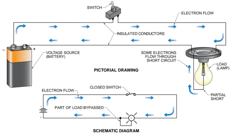
For PDC analysis is DC voltage step (amplitude U0) of some 100 V is applied between HW (high voltage) and LV (low voltage) windings during a certain time, the so-called polarization duration. Thus a charging current of the transformer capacitance, i.e. insulation system, the so called polarization current, flows. It is a pulse-like current during the instant of voltage application which decreases during the polarization duration to a certain value given by the conductivity of the insulation system. After elapsing the polarization duration, the switch goes into the other position and the dielectric is short circuited via the ammeter. Thus, a discharging current jumps to a negative value, which goes gradually towards zero. The simple measurement system of RVM method is shown in Fig.1 [6].

Fig.1. Principal scheme of RVM measurement system.

The RVM method consists of plotting the measured maximum response times with respect to the charging time, from which it is possible to determine the moisture content of the insulation in high-voltage oil equipment. In general, this method is intended for non-destructive, off-line determination of the state of the isolation system of transformers, cables or other devices that are comprised of the conductor and the insulator [7].

If the method is applied to an oil transformer, it determines the moisture content at the oil-paper dividing line. Measured values determine the time constant and the slope of the voltage response rise.

Based on the relationships listed in [8], paper moisture and conductivity in oil can be calculated with sufficient precision.

3. Introduced Measuring System for Determining Insulating State

The RVM method itself – measuring the voltage response of an insulating system, does not belong to Slovakia among the used methods. The proposal is based on the need to measure this method and because of the high cost of a narrowly specified commercial device. According to available information, this method is used in Slovakia only for measuring the insulation of the cables. Although this method was originally designed for cable diagnostics, its simplicity and precision in determining humidity is also applicable to high voltage electric machines.

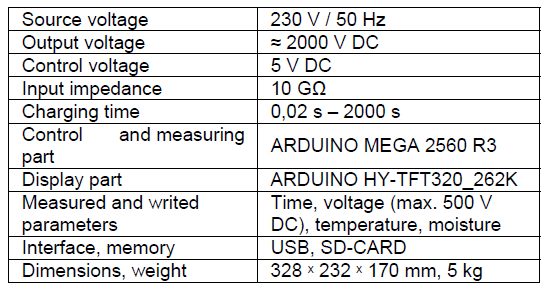
The proposed system can therefore be used to analyze the paper moisture state of power transformers. Parameters of the proposed measurement system for diagnostics of transformers are presented in Table 1.

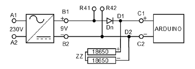
The source section of the device consists of two separate transducers. The main source for powering the ARDUINO platform is the rectifier from 230 VAC to 9 VDC / 2A. Despite the maximum supply voltage of 12 VDC, the output voltage of the stabilized voltage of 9 V is sufficient. The control voltage of the switching modules is from a separate inverter for protection. This voltage is at 5 VDC.

Fig. 2 shows a block diagram for the ARDUINO platform. This design also uses a back-up and at the same time a smoother source consisting of two series of connected 3.7 V batteries of type SJ 18650, each of which has its own protective charging circuit type TD1836.

TABLE I. PARAMETERS OF MEASURING SYSTEM BY RVM METHOD

.
Fig.2. Connecting of power supply to the measurement system platform.

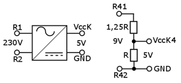
The control voltage of the switching modules is powered by a separate rectifier to protect the control panel. This voltage is at 5 VDC. In the Fig. 3 are a block diagram and a signaling of switch point source points and a voltage divider that supplies a switching module K4.

Fig.3. Power supply connecting of switching modules.

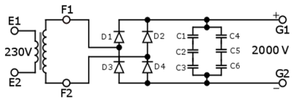
In order to protect the platform’s sensitive circuits and switch module control, both inverters are secured by a fuse. The high-voltage part of the measuring instrument is made of a single-phase transformer with an output voltage of 2100 V. This voltage is then guided by a bridge rectifier composed of four PRHVP2A-20 high-voltage diodes and a series-parallel connection of capacitors of the MKPI 337 type with a resulting capacity of 667 nF for reliable smoothing of the given run.

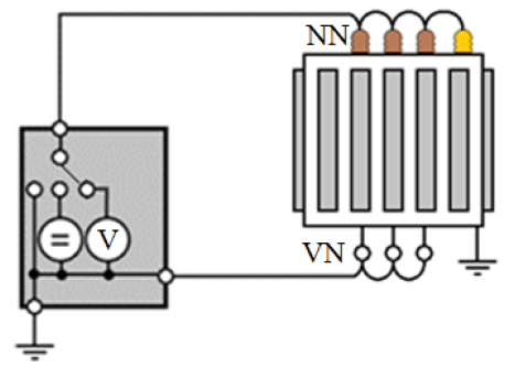
Since the proposed measuring instrument used to measure the voltage response of the transformer isolation system, that is to say, is connected between the coupled HV (high-voltage) and LV (low-voltage) windings, the load resistance is at the GΩ level. This high value is almost empty. Therefore, the output voltage when measuring 50 MΩ load with high voltage resistor can reach 2000 VDC. The diagram of the connection of the high voltage part is in Fig.4.

Fig.4. Connecting of high-voltage and rectifier part of the system.

Output voltage control, measurement and short-circuit connection are realized by ARDUINO switching modules controlled by 5 V voltage. Fig. 5 shows the connection and marking of the terminals.

Fig.5. Connecting of control and measured part for transformer 22/0.4 kV.

The switching module K1 consists of a series connection of SRD-05VDC-SL-C switching relays on a four channel switching module to achieve the required electrical strength. The left section of Fig.5 represents the normal no voltage state of the connection, therefore the terminals T1 and T2 are connected via the discharging resistance Rv.

To achieve a higher degree of safety, the switching modules K1, K2 and K3 are switched by the K4 module. This and switching module K3 ensures that, when switched on, in which no measurement is made, there is no dangerous voltage between terminals G1 and G2.

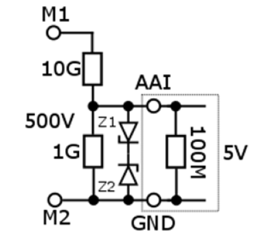
The measuring part of the instrument consists of the voltage divider shown in Fig. A serial connection of ten 1 GΩ precision measuring resistors is used to provide input 10 GΩ. This divider is a voltage at the platform input with a 100 MΩ input at a maximum of 4.95 V. If the input voltage between the M1 and M2 terminals exceeds 500 V (5 V between AAI and GND), the two Zener diodes Z1 and Z2 provide a secure upper the voltage limit.

Fig.6. Connecting of measuring input of platform ARDUINO.
4. Experimental Measurement and Diagnostics

The evaluation of the measurement and therefore the determination of the moisture content in the paper part of the isolation system of the oil transformer 22/0.4 kV can be determined from the analysis of the charging time and the maximum Umax voltage response according to Fig. 7 till Fig. 9.

For this evaluation, it is sufficient to write real time and measured voltage to the SD card. From this stored text document, time and voltage values are evaluated on a separate PC in one of the available computational programs. These text documents are named as rvmx, where x is the serial number of the measurement. For better orientation, the creation time is also indicated.

Measurement of the voltage response depends largely on the temperature difference between the object and the surroundings. Since the measured transformer is unconnected to the grid and is located in the laboratory, the temperature difference is zero [9]. This is confirmed by measuring the winding temperature on the transformer by incorporating the Neoptix temperature probes and measuring the outside temperature with a 22 ° C by thermometer.

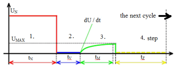
Measurement of return voltage by RVM consists of the four steps of Fig. 7 [10]. In the first step, the LV and HV transformer terminals are connected to the test voltage for the charging time tN. This step is called charging. In the second step, there is a discharge for tV = tN / 2, where the LV and HV terminals are short-circuited. In the third step, the measurement of the voltage response and the time itself is carried out until the maximum voltage is reached. The last fourth step of measuring the voltage response consists of a recovery before another cycle for a time at least equal to tN.

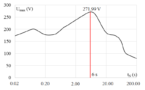
The time behaviour and the individual measurement steps are shown in the Fig. 7 and the graphical representation with the maximum value of the measured voltage response values, depending on the charging time, is shown in the Fig. 8.

The measurement of the voltage response of the insulation system consists of determining the moisture content of the paper part. This determination is derived from the characteristics of Fig. 9, which are obtained by actual measurements on samples of different humidity at different temperatures. These evaluation curves in another version are also reported in the literature [11].

Fig.7. The shape of the test voltage by RVM method.
Fig.8. The time behaviour of voltage response of the insulation system.
Fig.9. Evaluation curves for the voltage response measurement method.

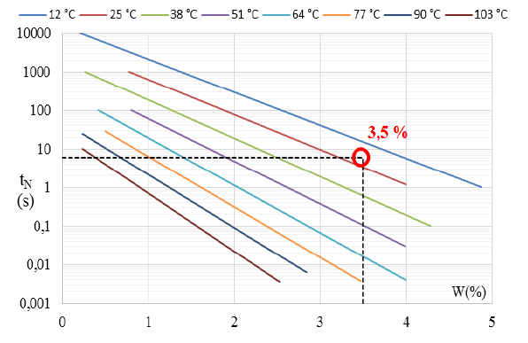
In Fig. 9 is shown the intercept point for moisture content of 3.5% corresponding to the highest possible moisture value in the paper section of the transformer insulation. Since the moisture content was also controlled by the dielectric spectroscopy with method of frequency response and the result of the evaluation was the same, it is obvious that no significant amount of sludge is deposited on the paper. The suspension itself in the transformer oil does not have a more serious effect on the result of this measurement.

Conclusion

This experimental analysis with designed system can be used as new system platform for determination of moisture in power oil transformer.

The proposed system, in comparison with other commercial devices, can evaluate the moisture status of paper part in the transformer insulation.

The measuring method RVM are unique in terms of analysis of insulating system of oil power transformers. In comparison with other methods, the RVM method can evaluate the moisture condition of the insulation paper of the power transformer with high accurate. This high reliability in determining moisture in paper was shown by determining the same result (3.5%) on the same measured distribution transformer as in case other method by frequency dielectric spectroscopy.

Precise determination of moisture content is very complex, because in the measured object in which the maximum voltage response is reached at shorter charging times, the moisture content of the insulation is higher. The maximum voltage response of the new transformers at lower moisture is achieved with longer charging times, what is the problem. From high accurate measurement it has been found a necessary to attach a sufficiently large high voltage (minimal from 2 kV).

Workers from individual test centres formulated their proposals and suggestions during the preparation phase as well as realization phase of the system development. After the system was brought into life, measurements of transformers became easier, safer and more accurate – in accordance with requirements from valid IEC standards.

This work was partially supported by the Grant Agency VEGA from the Ministry of Education of Slovak Republic under contract 1/0471/20.

REFERENCES

[1] Mentlík V. and et al., Diagnostics of electrical equipment, Prague: BEN, 2008, 439 pp., ISBN 978-80-7300-232-9.
[2] Monatanari G. C., Polarization and space charge behavior of unaged and electrically aged crosslinked polyethylene, In: IEEE Trans. Dielectr. Electr. Insul., vol. 7, pp. 474-479, 2000.
[3] Heatcote, M. J.,The J & P Transformer Book 13th edition, Chennai: ELSEVIER, 2007. p. 989. ISBN 978-0-7506-8164-3.
[4] Shayegani A. A., Hassan O., Borsi H., Gockenbach E., Mosheni H., PDC Measurement Evaluation On Oil-Pressboard Samples, In: International Conference on Solid Dielectrics, zv. 4, pp. 50-62, 2004.
[5] Petras J., Kurimsky J., Balogh J., Cimbala R., Dzmura J., Dolnik B., Kolcunova I., Thermally stimulated acoustic energy shift in transformer oil, Acta Acustica United with Acustica, 102(2016), No. 1, 16-22
[6] Leibfried T., Kachler A. J., Insulation Diagnostics on Power Transformers using the Polarisation and Depolarisation Current (PDC) Analysis, In: International Symposium on Electrical Insulation, zv. 10, pp. 170-173, 2002.
[7] Cimbala R., Kurimský J., Kolcunová I., Determination of Thermal Ageing Influence on Rotating Machine Insulation System Using Dielectric Spectroscopy, In: Przegląd Elektrotechniczny. Vol. 87, no. 8 (2011), p. 176-179. ISSN
0033-2097
[8] Kucera M., Sebok M., Electromagnetic compatibility analysis of electrical equipment’, In: DEMISEE 2016,” International conference Diagnostic of electrical machines and insulating systems in electrical engineering, Papradno, SR, 2016, p. 104-109.
[9] Brandt M., Identification failure of 3 MVA furnace transformer, DEMISEE 2016, International conference Diagnostic of electrical machines and insulating systems in electrical engineering, Papradno, SR, 2016
[10] Kúdelčík J., Hardoň Š., Varačka L., Measurement of Complex Permittivity of Oil-Based Ferrofluid in Magnetic Field, In: Acta Physica Polonica A, vol.131(4), pp. 931-933 (2017)
[11] Neimanis R., On Estimation of Moisture Content in Mass Impregnated Distribution Cables, Stockholm: Royal Institute of Technology Stockholm, 2001, ISSN 1100-1593
[12] Brandt M., Experimental measurement and analysis of frequency responses SFRA for rotating electrical machines, Elektroenergetika 2017, Stará Lesná, SR 284-288.
[13] Bartłomiejczyk M., Hamacek S., Kolosov D., Zharkov Y., Automated Diagnostics of Current Pick-Up Disturbances in Electric Traction Network’s, In: 14TH Intrnational Conference on Environment and Electrical Engineering (EEEIC), 2014.


Authors: Assoc. Prof. Milan Šimko, PhD.; Assoc. Prof. Daniel Korenčiak, PhD.; Prof. Miroslav Gutten, PhD.; Ing. Richard Janura, PhD.; Faculty of Electrical Engineering and Information Technology of the University of Žilina Department of Measurement and Applied Electrical Engineering, Univerzitná 1, 010 26 Žilina, Slovak Republic, E-mail:gutten@fel.uniza.sk.


Source & Publisher Item Identifier: PRZEGLĄD ELEKTROTECHNICZNY, ISSN 0033-2097, R. 96 NR 12/2020. doi:10.15199/48.2020.12.12

How to Reduce the Soil’s Resistivity

Published by Lorenzo Mari, EE Power – Technical Articles: How to Reduce the Soil’s Resistivity, September 28, 2020.


Lowering the resistance of a grounding electrode is not always enough to reduce the soil’s resistivity. Reducing the resistivity of the soil around the electrodes can help achieve adequate resistance to the ground.

The elements that most affect the soil resistivity are moisture content, ionizable salts, and porosity. Water and ionizable salts combine to form an electrolyte, which is a conductor of electricity. Porosity is an indicator of the ability of the soil to retain the electrolyte.

Some methods to reduce the soil resistivity include:

Water retention
Chemical salts
Bentonite
Chemical-type electrodes
Ground enhancement materials

Water Retention

Most soils lose moisture when they receive direct sunlight. The sun heats the ground and causes the water contained in it to rise to the surface and vaporize, dispersing in the atmosphere. The longer the heating process, the drier the soil.

Excessive drainage can also quickly leach away the salts in the soil and dry out the deeper layers.

The water molecules ionize the minerals in the soil and cause them to become conductive. Without moisture, an electrical connection to earth is not possible. Figure 1 shows how the resistivity varies as a function of moisture content for various types of soil.

Figure 1. Soil resistivity and moisture content

As observed, there is a strong association between the water content and the resistivity of soils. The best soil types require a minimum of 4% water (by weight), while the poorest require at least 14%.

Some areas of the world have soils with more than enough moisture. Others, however, have none. Deserts are mainly arid and have little to no soil moisture. A simple standard copper rod will not serve as a ground connection in these places unless water is added to the soil.

The soil may or may not retain an appropriate amount of moisture, according to its degree of porosity. This condition directly impacts both the distribution of the content of ionizable salts and the formation of the electrolyte. Improving the soil’s ability to retain moisture is an effective way to decrease its resistivity.

Where there is no moisture, providing it will achieve reasonable grounding. It is only required to moisten the soil near the grounding electrode. For the best results, the electrode/soil interface should be wet.

An infrequent but effective way to maintain soil moisture is to plant vegetables around the grounding electrodes. Vegetables retard runoff and retain irrigation water and salts in the soil, helping to keep the area moist and the salts dissolved. 

An irrigation system is also helpful in keeping the soil moist. The installation of an automatic moisture sensing and water supply system, in combination with a conventional water supply system, can precisely control the moisture content of a given soil.

Chemical Treatments

The use of ion-producing chemical compounds like sodium chloride, magnesium sulfate (epsom salt), copper sulfate (blue vitriol), and calcium chloride around the grounding electrodes, decreases the soil’s resistivity and the electrode’s resistance to ground.

The most widely-used chemical is magnesium sulfate. It is low-cost, has strong electrical conductivity, and has little corrosive effect.

Ordinary rock salt is cheap. Common salt (sodium chloride) is highly corrosive. This corrosive effect may cause nearby metal objects to deteriorate. Despite being an excellent conductor of electricity, its adverse effects remove it from the list of preferred chemicals.

The chemical treatment indirectly increases the diameter of the electrode by modifying its surrounding soil. When the soil is porous, the solution permeates quickly into a large volume of earth, making a large equivalent diameter, with quick results.  In contrast, when the soil is compact, the chemicals take time to spread, and results are produced more slowly.

A practical way of applying these compounds is through a circular trench excavated around the ground rod, preventing direct contact with the electrode (Figure 2). 

Figure 2. Soil treatment with a circular trench. Image based on a drawing from  IAEI.

It can be beneficial to supply a little water through a pipe to accelerate the effect of the salts. The amount of water should be sufficient to keep the area  moist, but without washing away the salts.

The chemicals are gradually washed away by natural drainage through the soil and rainfall, requiring periodic replacements. The period for replacement varies depending on site conditions, but it may be years. An adequate maintenance scheme will ensure that chemicals will have long-lasting effects.

A particular characteristic of the chemical treatment is the reduction of seasonal variations of the resistance to ground. These variations come from the periodic drying and wetting of the soil.

Use caution, as local authorities may prohibit the use of chemicals if they are not considered environmentally friendly.

Bentonite

Adding bentonite to the soil reduces its resistivity and the ground resistance of the electrodes.

Bentonite is a fine-grained, highly plastic clay, formed by volcanic action. It may be used as soil replacement and filler material for electrical grounding in places with high resistivity. The conductive Bentonite clay is a sodium activated montmorillonite. Bentonite is chemically hydrated, innately stable, and retains its properties over time.

Bentonite absorbs moisture from the surrounding soil and swells up to several times its dry volume. It adheres to the surface of the grounding rods and cables laid in trenches, reducing the contact resistance and increasing their diameter artificially.

The resistivity of bentonite depends on the water content. The water inside the pores allows the electrical currents to move through the bentonite. The resistivity value is lower in the liquid state than in the plastic or solid state and is on the order of 250 Ω∙cm at 300% moisture.

In addition to reducing the resistance to ground of rods and cables, the moisture retention process of the bentonite compound protects against corrosion.

Bentonite performance is highly dependent on the amount of rainfall, soil moisture, and temperature at the site. In hot climates, the soil dries out, and the bentonite does not work as desired. It may separate from the electrodes, increasing the resistance to the ground.

Chemical Rods

Chemical rods are suitable for high resistivity soils — rock, mountain tops, sandy soil — and places with excessively high or low temperatures.

This type of rod is a tube filled with mineral salts distributed evenly.  It has holes along its length, allowing the entry of soil moisture. The moisture combines with the salts and dissolves them. The saline solution then seeps out through the holes and soaks into the surrounding soil, continuously conditioning a large volume around it.

The materials available are copper, stainless steel, and hot-dipped galvanized iron. Its length choices are the same as conventional rods: 240 cm (8 ft) and 300 cm (10 ft).

They may be installed by drilling holes in the ground, and, for rocky soils, manufacturers offer horizontal rods. It is customary to place a grounding enhancement fill around the rod to improve the interface with soil.

These rods also require maintenance. For this, they have a removable cap for inspection and chemical supply (Figure 3).

Figure 3. Chemical rod. Image courtesy of Lightning Eliminators
Grounding Enhancement Fill

Replacing all or part of the soil around an electrode with a low resistivity filler will facilitate the achievement of low ground resistance. The higher the percentage of earth swapped, the lower the ground resistance.

A grounding enhancement fill may have resistivities as low as 50 Ω∙cm (much lower than bentonite). It works in a trench, around a ground rod or substation grounding conductors, either dry or in a slurry.

The main properties are: constant resistance, low resistivity, maintain moisture, stability, low freezing point, resistance to leaching, non-corrosive, and maintenance-free.

Reviewing How to Reduce the Soil’s Resistivity

When the grounding electrode does not achieve a low enough resistance, another option is to reduce the resistivity of the soil. There are several methods to accomplish this: water retention, chemical salts, bentonite, chemical-type electrodes, and ground enhancement materials.

While all methods are effective, the selection will depend on the site’s particular conditions and the ability to carry out proper maintenance when required.


Author: Lorenzo Mari holds a Master of Science degree in Electric Power Engineering from Rensselaer Polytechnic Institute (RPI). He has been a university professor since 1982, teaching topics as electric circuit analysis, electric machinery, power system analysis, and power system grounding. As such, he has written many articles to be used by students as learning tools. He also created five courses to be taught to electrical engineers in career development programs, i.e., Electrical Installations in Hazardous Locations, National Electrical Code, Electric Machinery, Power and Electronic Grounding Systems and Electric Power Substations Design. As a professional engineer, Mari has written dozens of technical specifications and other documents regarding electrical equipment and installations for major oil, gas and petrochemical capital projects. He has been EPCC Project Manager for some large oil, gas & petrochemical capital projects where he wrote many managerial documents commonly used in this kind of works.


Source URL: https://eepower.com/technical-articles/how-to-reduce-the-soils-resistivity/

Electromagnetic Disturbances Propagation Along a Grounding Grid Subjected to Lightning Currents

Published by Rafael ALIPIO, Renan SEGANTINI, Federal Centre of Technological Education of Minas Gerais


Abstract. This paper assesses the transient distribution of potentials along a grounding grid subjected to currents representative of first and subsequent strokes. It is shown that the transient non-uniform distribution of potential along the grounding system may lead to the flow of impulsive current between pieces of equipment grounded at distinct points. The methodology presented in this paper is useful in determining engineering actions to reduce the risks of electromagnetic disturbances propagation due to uneven potential distribution along grounding grids.

Streszczenie. Obliczono chwilowe rozkłady potencjałów w uziomie kratowym podczas odprowadzania prądów piorunowych pierwszego i kolejnych wyładowań głównych. Nierównomierny rozkład potencjału może prowadzić do przepływu prądów impulsowych pomiędzy urządzeniami uziemionymi w różnych punktach. Metoda jest użyteczna do ustalenia środków redukujących zagrożenie związane z nierównomiernym rozkładem potencjału w systemie uziomowym. (Propagacja zaburzeń elektromagnetycznych w uziomie kratowym podczas odprowadzania prądów piorunowych).

Keywords: lightning response of grounding, transient analysis of grounding, transient potential distribution, multiport wideband model.
Słowa kluczowe: odpowiedź uziomu na udar piorunowy, analiza uziomu w stanie nieustalonym, chwilowy rozkład potencjału, szerokopasmowy model wielowejściowy.

Introduction

Extended meshed earthing systems, called grounding grids, are commonly used in large installations, such as substations, to protect and safeguard personnel and equipment against the hazards and devastation that may be caused by the flow of fault currents [1]. They also provide reference voltages for electrical and electronic systems.

The grounding grids are usually designed considering only low-frequency occurrences (50/60-Hz ground-fault currents) [2]. However, the transient response of grounding grids may be also important, for instance, when they are fed by lightning currents [3]. This can occur when lightning directly strikes the substation components or when it strikes spans of power lines near the substation. In both cases, a noticeable portion of the current is driven to the ground.

When subjected to lightning currents, the grounding grid response presents certain complexities that make its behaviour quite different from that presented at low frequency [4]. Due to the impulse nature of lightning currents, they present a wideband frequency content ranging from dc to several MHz. In this frequency range, the grounding system shows different behaviour at different frequency intervals. Among other aspects, this frequency dependent behaviour of grounding leads to an uneven potential distribution along the grounding grid [3].

The non-uniform distribution of potentials along the grounding grid may be source of electromagnetic disturbances. For instance, it is common in modern substations or industrial plants the existence of electrical panels in the control room that are responsible for remote commanding the operation of some equipment installed in the substations yard. In many cases, the equipment and the panel are grounded at distinct points of the grounding system (see Fig. 1 of reference [3]). Hence, when the grounding is subjected to lightning currents, the resulting non-uniform distribution of potentials may cause the flow of impulsive currents through the closed path between the equipment at the substation yard and the electric panel at the control room. Such loop currents are source of electromagnetic disturbances, causing equipment malfunctions, failures and damage.

The objective of this work is to make a sensitivity analysis of the potential distribution in a grounding grid subjected to impulsive currents. The present paper is an extension of the previous analysis developed by the first author in [3], considering two main new aspects. First, in order to simulate the wideband behaviour of the grounding grid, an accurate multiport model is developed, which can be promptly included in widespread time-domain electromagnetic transient tools, such as ATP-EMTP, EMTPRV, and PSCAD. This multiport model allows simulating the grounding system in conjunction with the substation components, and is suitable for developing accurate electromagnetic transient studies using time-domain tools. Secondly, realistic lightning current pulse waveforms are used, which reproduce the observed concave rising portion of typical measured lightning currents.

Modelling of grounding systems

As mentioned, lightning currents present a wideband frequency content ranging from dc to several MHz. Therefore, to develop accurate analysis of the transient response of grounding systems, their frequency-dependent behaviour should be considered. To this aim, a wideband model of the grounding grid is obtained as briefly described in next paragraphs.

The wideband response of the grounding grid is determined using the accurate Hybrid Electromagnetic Model (HEM) [5], in a frequency range from dc to several megahertz. In particular, HEM is used to determine the grounding admittance matrix Yg(s) over the frequency range of interest [6]. The grounding admittance matrix physically relates the vector of nodal voltages of grounding system and the vector of injected current into each grounding node. The Hybrid Electromagnetic Model solves Maxwell’s equations numerically via the vector and scalar potentials using the thin wire approximations [5]. The calculations are performed in frequency domain and, if required, time domain results can be obtained by means of inverse Fourier or Laplace transform. The accuracy of the results provided by this model in terms of the impulse response of grounding was proved by comparison with experimental results, considering different grounding arrangements (for instance, horizontal electrodes and rods in [7] and large grids in [8]).

After calculating the frequency response of the grounding grid, a pole-residue model of the calculated nodal admittance matrix Yg(s) is obtained. The objective is to calculate a pole-residue model (1) which approximates (“fits”) the original data as close as possible.

.

In case of a physical system, the admittance matrix Yg(s) is symmetrical. Hence, Rm, D and E are also symmetric, being D and E real matrices. In this work, E is set equal to zero, D is related with the low-frequency response of grounding and the sum of rational functions represents the frequency response of grounding. The approximated model Yfit fits the results calculated using the accurate electromagnetic model.

To obtain a pole-residue model (1), the Vector Fitting (VF) technique is used [9]. First, the pole-residue model of the grounding system admittance matrix is obtained. Then, in order to obtain stable time-domain simulations, the passivity is enforced by perturbation of model parameters. Further details regarding the VF and the passivity enforcement by perturbation can be found in [9, 10].

Finally, once the passive pole-residue model of the grounding system admittance matrix is obtained, it can be represented in the form of an electrical network, which can be promptly included in time-domain simulations. Considering this approach, the rational functions can be easily converted into basic network elements (R, L, C). The network has branches between all nodes and ground, representing the diagonal elements of Yfit, and between all nodes, representing the off-diagonal elements of Yfit. Once determined the equivalent electrical network, it can be imported directly into time-domain electromagnetic transient tools.

Developments

We consider a square grounding grid of 60 m x 60 m, composed of square meshes with space between conductors of 5 m, as depicted in Fig 1. The conductors are constructed from copper with 7-mm radius and the grid is buried at a depth of 0.8 m in a uniform soil. There different values of soil resistivity ρ are considered, 300, 1000 and 3000 Ωm, comprising low, moderate and high values of resistivity. The relative permittivity is assumed εr=10 and the relative permeability is assumed μr=1. In a conservative approach, the frequency dependence of the electrical parameters of soil is neglected [7].

Fig.1. Tested grounding grid. Cartesian coordinates: A(55, 55)m; B(30,45)m

In this study we have used two lightning current waveforms corresponding to the typical first and subsequent return strokes, based on observations of Berger et al. [11], according to [12], Fig. 2. The current waveforms are chosen by Rachidi et al. [12] to fit typical experimental data and are reproduced by means of a sum of Heidler’s functions [13]. It should be stressed that subsequent stroke, which has larger rate of rise of the front, has higher frequency content in comparison with the first stroke, as mentioned in [14]. On the other hand, first stroke currents have larger energy content, due to their higher amplitude and longer duration, in comparison with subsequent strokes.

It is assumed that the discharge directly strikes the lightning protection system of the substation and the current is distributed by down-conductors through the four corners of the grid. The resultant Grounding Potential Rise (GPR) developed in points A and B of the grid, see Fig. 1, are then calculated.

The multiport wideband model of the grounding system was obtained according to Section II. It is worth mentioning that both the pole-residue model and the electrical network were obtained using the public domain calculation package for rational approximation of frequency dependent admittance matrices available in [15]. All time-domain simulations presented in the next sections were developed in the Alternative Transients Program (ATP) [16].

Fig.2.

Fig.2. The first return-stroke current pulse is characterized by a peak value of 30 kA, zero-to-peak time of about 8-μs and a maximum steepness of 12 kA/μs, whereas the subsequent return stroke current has a peak value of 12 kA, zero-to-peak time of about 0.8-μs and a maximum steepness of 40 kA/μs

Results of Grounding Potential Rise (GPR)

Before analyzing the results, it is important to state some basic aspects concerning the propagation of current and voltage waves along buried bare conductors in soil. The wave propagation is dictated by the medium propagation constant, which is given approximately by

.

for a given angular frequency ω. In particular, the attenuation of the wave is related with the real part of the propagation constant, called attenuation constant (α). It increases with frequency and with medium conductivity. Thus, larger attenuation of voltage and current waves propagating along bare conductors buried in soils of higher conductivity (lower resistivity) is expected. Similarly, current and voltage pulses of shorter front times are expected to suffer stronger attenuation, due to their higher frequency content.

Figs. 3, 4 and 5 illustrates the GPRs developed in points A and B respectively for soil resistivity of 300, 1000 and 3000 Ωm, in response to current pulses representative of (a) first and (b) subsequent strokes. Based on the results, two main periods can be distinguished in the transient behavior of grounding grid: 1) a fast transient period and 2) a slow transient period.

In the fast transient period, the propagation and inductive effects are pronounced. In this period, the distribution of potentials along the grounding grid is not uniform, since the voltage wave experiences a strong attenuation as it propagates from the current impression points. In the analysed case, the non-uniform potential distribution is related with the transient potential difference between earth terminations A and B, vAB(t). In order to state a criterion to judge whether the potential distribution is more or less uniform, the ratio between the peak value of vAB(t) and the peak value of the transient potential developed in point A, vA(t), is calculated. The larger this ratio, the more non-uniform the potential distribution. Considering the results of Figs. 3, 4 and 5, for soils of 300, 1000 and 3000 Ωm, the ratios between the peaks of vAB(t) and vA(t) are around 37% and 99%, 13% and 92%, 4% and 45%, respectively for first and subsequent strokes. Thus, the more conductive the soil is, the more the potential distribution is non-uniform. This is due to the fact that the attenuation effects are much more significant in soils of higher conductivity. Furthermore, note that the differences between the curves of GPR along the fast transient period are more pronounced in case of subsequent strokes, due to their higher frequency content in comparison with first stroke currents.

Fig.3. GPRs developed in points A and B for a soil resistivity of 300 Ωm in response of currents representative of (a) first and (b) subsequent strokes
Fig.4. Same of Fig. 3, but for a soil resistivity of 1000 Ωm
Fig.5. Same of Fig. 3, but for a soil resistivity of 3000 Ωm

In the slow transient period, the GPR curves of points A and B present a similar behaviour and are basically coincident, indicating that all the points of the grounding grid are at the same potential. This behaviour is associated with the tail of the impressed current waves, which contain the low-frequency components of the current. Thus, during this period the propagation and inductive effects are negligible and the grounding grid presents a uniform potential distribution and can be assumed to be equipotential across its area.

Results of Impulsive Loop Currents and Energy Dissipated

Figs. 6-8 illustrate the transient potential difference between earth terminations A and B, vAB(t), respectively for soil resistivity of 300, 1000 and 3000 Ωm, considering both (a) first and (b) subsequent strokes.

Fig.6.

Fig.6. Transient potential difference between earth terminations A and B for a soil resistivity of 300 Ωm, considering the impression into the grounding grid of current pulses representative of (a) first and (b) subsequent strokes

Fig.7. Same of Fig. 6, but for a soil resistivity of 1000 Ωm
Fig.8. Same of Fig. 6, but for a soil resistivity of 3000 Ωm

It can be seen that, along the fast transient period, the potential differences between the two earth terminations are significant and present short rise-time, mainly in case of subsequent strokes. Such potential differences may lead to the flow of impulsive loop currents between equipment grounded at distinct earth terminations and connected among each other, for instance, by control or communication cables. Along the slow transient period, there is no current flowing between the equipment, since, there is no potential difference within the grid area (the grid is at a constant potential).

The heating resulting from the energy dissipated while the loop current flows into and through a “victim” circuit is the source of damage. The lightning parameter that is most closely related to this effect is the specific energy or action integral [17]. The response of a “victim” is represented by its equivalent resistance. The dissipated energy, and therefore associated damage, can be roughly estimated as the product of the specific energy by this resistance [17].

In order to make a first assessment of the damage caused by the flow of loop currents, Fig. 9 illustrates the energy dissipated considering the application of the voltages depicted in Figs. 6-8 to a normalized equivalent resistance of 1 Ω. The figure also includes results of further simulations developed for the same grounding system buried in a soil of 100 Ωm.

It can be seen from Fig. 9 that the trend of higher energy dissipation in case where the grid is fed by currents of first strokes is inverted with increasing the soil resistivity. This interesting finding can be explained as follows. Due to the propagation characteristics in high-resistivity soils (lower attenuation and higher propagation velocity), the potential distribution is more uniform along the grounding grid in case of first stroke currents, which present lower frequency content in comparison with subsequent strokes. Thus, in spite of the higher energy content of first stroke currents, in case of grounding systems buried in soils of high resistivity, the energy dissipated by impulsive loop currents tends to be more pronounced considering subsequent currents striking the substation.

Fig.9.

Fig.9. Energy dissipated considering the application of the voltages depicted in Figs. 6-8 to a normalized equivalent resistance of 1 Ω, including additional simulations for the same grid buried in a soil of 100 Ωm

Summary and conclusions

This paper assessed the transient distribution of potentials along a grounding grid subjected to currents representative of first and subsequent strokes. The methodology presented in this paper is useful in determining engineering actions to reduce the risks relative to the non-uniform potential distribution along grounding grids when subjected to lightning currents. Considering the grid analyzed in this paper, one practical measure consists of connecting the two distinct earth grounding points with an aerial conductor to a metal bar, preferably located at the midpoint between the two points. Then, this bar is connected to the earth grounding grid by means of a proper conductor. Depending on the configuration of the power plant this solution is not always feasible due to physical limitations, or even due to cost constraints. In such cases, it is essential to know the distribution of potentials along the earth grounding grid, especially when it is subjected to lightning currents, in order to define alternative solutions. In particular, the proper installation of surge protective devices at the terminal of sensitive equipment can be done based on the accurate knowledge of the transient potential distribution along the grounding grid.

This work was supported in part by The State of Minas Gerais Research Foundation (FAPEMIG), under grant TEC – APQ-02017-16.

REFERENCES

[1] L. Grcev, Transient Electromagnetic Fields Near Large Earthing Systems, IEEE Trans. Magnetics, 32 (1996), No. 3, 1525–1528.
[2] IEEE Guide for Safety in AC Substation Grounding, IEEE Std.80 (2013).
[3] R. Alipio, M. A. O. Schroeder, and M. M. Afonso, Voltage distribution along earth grounding grids subjected to lightning currents, IEEE Trans. Industry Applications, 51 (2015), No. 6, 4912–4916.
[4] S. Visacro, A comprehensive approach to the grounding response to lightning currents, IEEE Trans. Power Delivery, 22 (2007), No. 1, 381–386.
[5] S. Visacro and A. Soares Jr., HEM: a model for simulation of lightning-related engineering problems, IEEE Trans. Power Delivery, 20 (2005), No. 2, 1026–1208.
[6] R. Alipio and Fellipe M. S. Borges, Multiport wideband modeling of large substation grounding grids for transient analysis, in Proc. 10th Asia-Pacific International Conference on Lightning (2017), 313–317.
[7] R. Alipio and S. Visacro, Impulse efficiency of grounding electrodes: effect of frequency dependent soil parameters, IEEE Trans. Power Delivery, 29 (2014), No. 2, 716–723.
[8] S. Visacro, R. Alipio, C. Pereira, M. Guimarães, and M. A. O. Schroeder, Lightning response of grounding grids: simulated and experimental results, IEEE Trans. Electromagnetic Compatibility, 57 (2015), No. 1, 121–127.
[9] B. Gustavsen and A. Semlyen, Rational approximation of frequency domain responses by vector fitting, IEEE Trans. Power Delivery, 14 (1999), 1052–1061.
[10] B. Gustavsen, Fast passivity enforcement for pole-residue models by perturbation of residue matrix eigenvalues, IEEE Trans. Power Delivery, 23 (2008), No. 4, 2278–2285.
[11] K. Berger, R. B. Anderson, and H. Kroninger, “Parameters of
lightning flashes,” Electra, no. 41, pp. 23–37, 1975.
[12] F. Rachidi, W. Janischewskyj, A. M. Hussein, C. A. Nucci, S. Guerrieri, B. Kordi, and J.-S. Chang, “Current and electromagnetic field associated with lightning-return strokes to tall towers,” IEEE Trans. Electromagn. Compat., vol. 43, no.3, pp. 356–367, Aug. 2001.
[13] F. Heidler, “Analytische blitzstromfunktion zur LEMPberechnung,” in Proc. 18th Int. Conf. Lightning Protection, Munich, Germany, 1985, pp. 63–66.
[14] L. Grcev, “Impulse efficiency of ground electrodes,” IEEE Trans. Power Del., vol. 24, no. 1, pp. 441–451, Jan. 2009.
[15] B. Gustavsen, Matrix Fitting Toolbox [Online]. Available: https://www.sintef.no/projectweb/vectfit/, 2009.
[16] L. Prikler, H.K. Hoidalen, ATPDraw Manual, Version 5.6, 2009.
[17] CIGRE Lightning Parameters for Engineering Applications, Working Group C4.407, Aug. 2013.


Authors: prof. Rafael Alipio, Department of Electrical Engineering, Federal Center of Technological Education of Minas Gerais, Av Amazonas, 7675, postal code: 30510000, Belo Horizonte, Brazil , E-mail: Rafael.Alipio@des.cefetmg.br; Renan Segantini, E-mail: renan_nikel@hotmail.com.


Source & Publisher Item Identifier: PRZEGLĄD ELEKTROTECHNICZNY, ISSN 0033-2097, R. 94 NR 2/2018. doi:10.15199/48.2018.02.02

Influence of Distributed Generation on Sectionalizing Switches Placement in MV Distribution Networks

Published by Wojciech BĄCHOREK1, Mariusz BENESZ1, AGH University of Science and Technology (1)


Abstract. This paper presents the influence of distributed generation DG and reclosers placement on the reliability of distribution network. The brute force method and evolutionary algorithm were used to solve the optimization task. The placement of the switches was determined independently using two criteria. The first criterion is the reserve factor, while the second criterion is the SAIDI index. The proposed methods were tested on a real medium voltage distribution system in two variants of operation: with and without DG.

Streszczenie. W artykule przedstawiono wpływ generacji rozproszonej i lokalizacji reklozerów na niezawodność sieci dystrybucyjnej. Zastosowano algorytm przeglądu zupełnego oraz algorytm ewolucyjny. Lokalizację reklozerów ustalono stosując dwa kryteria: współczynnik rezerwowania oraz wskaźnik SAIDI. Obliczenia zrealizowano dla rzeczywistej sieci średniego napięcia. (Wpływ generacji rozproszonej na rozmieszczenie łączników sekcjonujących w sieci średniego napięcia).

Keywords: distribution networks reliability, reclosers, SAIDI, distributed generation.
Słowa kluczowe: niezawodność sieci dystrybucyjnych, łączniki sekcjonujące, SAIDI, generacja rozproszona.

Introduction

One of many important optimization problems solved for distribution networks is the sectionalizing switches placement problem (SPP). This problem is still very important due to the growing popularity of distributed generation sources (DG). Distributed generation improves voltage levels, reduces power losses and improves reliability of the network [1, 2, 3]. Sectionalizing switches, that allow network reconfiguration, should be placed taking into account DG sources. Reconfiguration efficiency is ensured by reclosers [4, 5] and remote-controlled switches [6, 7].

Different methods and objective functions are used to solve the SPP problem. Calculation methods of solving SPP problem may be divided into two groups: based on the classical mathematical methods (for example the mixed integer linear programming [1, 8] or the fuzzy method [9]) and based on the heuristic methods (for example the ant colony optimization algorithm [3, 4, 10], the genetic algorithm [5, 10, 11], the particle swarm optimization method [12, 13] or the taboo search algorithm [14]). Regardless of the calculation method applied, objective functions based on different criteria are assumed. The most applied objective functions are cost criterions and reliability indices. The cost of the switches is taken into account in the articles [3, 4, 12, 14]. The authors of the papers [8, 15] took into account the maintenance costs of switches. In [11], the impact of the cost of DG sources on the placement of sectionalizing switches was considered. SAIDI, SAIFI indices are considered in [4, 9]. The main task of the article is to analyze the placement of sectionalizing switches in the real distribution network with DG. This analysis was carried out independently using two criteria: reserve factor ρ [16, 17] and SAIDI index [4, 9].

The solution sought should correspond to the highest or smallest value of the objective function, respectively for the first and the second criterion. Regardless of the criterion applied, a brute force method and an evolutionary algorithm were used.

First of all, the optimization problem was formulated – the benefits from the installation of sectionalizing switches and the impact of distributed generation on reliability were presented. Next, a description of solution method based on the evolutionary algorithm and a computational example are presented. The calculations were carried out separately for the two selected criteria. In each case, three levels of DG were taken into account.

Problem formulation

A. Idea of sectionalizing switches installation

An example of a simple distribution network is shown in Fig. 1. This is a typical medium voltage power line. Two sectioning switches divide the network into three sections called X, Y and Z. An additional power supply (DG) is connected to the Z section.

Fig.1. The idea of installing sectionalizing switches.

In case of a failure, different scenarios of shutdowns in the network are possible. The first scenario concerns the situation when it is not possible to provide back-up power to the network by closing a switch normally open at the tie point (power supply from MFP B). The second scenario, unlike the first one, assumes the possibility of supplying backup power to the line. In both scenarios, the possibility of a back-up supply using DGs could be considered. This may mean supplying a part of the network only from an additional source (island operation in first scenario) if the load demand of the section to which the DG is connected does not exceed the DG capacity.

In case of a failure of e.g. Y section, the recloser separating X and Y sections is opened and disconnects from the power supply of Y and Z sections. Then, after opening the switch between the Y and Z sections, it is possible to restore power to the Z section. This is possible in the second scenario or in the first scenario with adequate DG capacity.

The proper placement of switches is therefore an important optimisation problem for distribution networks. Sectioning switches ensure reduction of energy not supplied (ENS) [15] to customers and improvement of network reliability indices, which are of interest to Distribution System Operators (DSO).

B. Reserve factor

One of the many criteria for selecting optimal sectionalizing switch placements is the reserve factor ρ (1). This factor was defined and applied in the calculations described e.g. in works [16, 17].

.

where: E – sum of all customers’ energy in the network, Ei – energy of customers who have been disconnected as a result of a failure in i-th section, NS – number of all sections in the network, NBi – number of branches in the i-th section, λij – average failure rate of j-th branch in i-th section, rij – average outage time of j-th branch in section i.

The minimum value of the reserve factor is 0. The maximum value of the factor is 1. The solutions with the highest reserve factor shall be selected from among all the solutions of the switch placement.

C. SAIDI

The objective function of placement of switches in the distribution network may also be SAIDI index. SAIDI is one of the basic reliability indices used by DSO. This index is calculated and published by DSO on the basis of registered power interruption incidents. SAIDI is an index of an average system duration outages in the supply of electricity expressed in minutes per customer per year. This is a sum of the interruption duration multiplied by number of customers exposed to the effects of the interruption during the year, divided by the number of customers connected to the network (2). Among all the solutions of the switch placement, a solution with the lowest SAIDI value is selected.

.

where: NK – number of power delivery points, Nk – number of customers in k-th power delivery point, Uk – annual duration of unscheduled interruptions in k-th point.

The annual duration of unscheduled interruptions Uk is given by (3):

.

where: NC – total number of possible fault locations, λi – average failure rate of distribution elements grouped together (section), ri – average outage time of distribution elements grouped together.

Index (2) was calculated with a statistical approach based on combinatorial reliability analysis. Dedicated software developed by the authors takes into consideration: the types of sectionalizing switches, their locations and the possibilities of the alternative supply of the line.

Calculation method

In order to determine optimal switch placements, two calculation algorithms were used. If a small number of switches (1 or 2 switches) were assumed, a brute force method (complete overview of the solutions) was carried out. An evolutionary algorithm was used to locate at least 3 sectionalizing switches. This has resulted in a reduction of the calculation time. The solution of a task is written in a form that is “elgible” to the evolutionary algorithm. This is realized with the use of the real coding method.

The solution is expressed in a sequence of numbers called a chromosome (Fig. 2). The number of string elements is equal to the number of placed switches (SN). The location of the switch (SL) in the network is determined at each position of the string in the form of a suitable index.

Fig.2. Chromosome structure

Their initial population (specified in number) is random. The evolutionary operators are elaborated for creating new solutions. The selection, crossover and mutation operators were used. Stochastic sampling with replacement mechanism was used in the selection procedure. The procedure of a one point crossover of individuals was applied.

The calculations were made using the computer program written in the C ++ programming language.

Case studies

A. The examined MV distribution network

The proposed method is tested on 15 kV modified real-life distribution network located in Poland [17]. The system with 87 MV/LV substations is shown in Fig. 3. This system has 348 possible sectionalizing switches locations. The installation of reclosers is assumed. The total length of the power line is 74.73 km while the lateral branches are 51.98 km. The total peak load 4134 kW. There are 1152 customers connected to the network. The failure rate of MV branches is λ = 0.08 f/yr.km and the mean time to repair is r = 3.83 h/f.

The calculations were carried out in two variants. The first variant assumes that it is not possible to provide backup power to the network by closing the normally open switch. The second one allows such a possibility. Additionally, in a selected point of the network, the connection of a dispersed generation was allowed. The following three power sources were considered: PG1 = 630 kW, PG2 = 1105 kW, PG3 = 2066 kW. These variants of the DG were named respectively G1, G2 and G3. The variant without DG was named as G0.

There are two tie points in the network. They provide the possibility of back-up power supply for the analysed network by closing the normally open switch (tie point). The size of the reserved network depends on the type and place of failure and the number and location of sectionalizing switches. In the power line (Fig. 3) it is not possible to provide backup power to the entire network via a tie points. For more information on backup power limitations, see [17]. In order to solve the task of sectionalizing switches placement, two criteria were applied independently: the maximizing the value of the reserve factor and the minimization of SAIDI. Two scenarios related to the possibility of back-up power supply are being considered:

• scenario I: it is not possible to provide back-up power to the network by closing a switch normally open at the tie point (with and without DG),

• scenario II: backup power supply is possible by closing the switch at the tie point (with and without DG).

The analysed MV power line meets the requirements of the DSO with respect to current load capacity and voltage levels. These requirements are described in the work [17]. The following evolutionary algorithm parameters were chosen: size of population = 24, crossover probability = 0.8, mutation probability = 0.03, number of generations = 3000.

Fig.3. Diagram of analyzed MV power line

B. Analysis of calculation results

In this chapter, the results of the placement of the reclosers are presented. Calculations were made for two previously described scenarios, in each of them for different number of reclosers. The placement of 1 to 8 switches was assumed. The optimal placement of the switches was determined independently for both criteria ρ (1) and SAIDI (2). The location of the DG source in the medium voltage power line is shown in Fig. 3.

For the analysed network without sectionalizing switches, the reserve factor ρ = 0, SAIDI = 1329.2 min/cus.y. and ENS = 575.5 MWh.

The optimum sectionalizing switch placements according to scenario I for networks without and with DG source have been presented in Table 1. The values of SAIDI have been also shown in Fig. 4.

Table 1. Results of the sectionalizing switch placement (scenario I)

.

Table 2. Results of the sectionalizing switch placement (scenario II)

.

The optimum placements of reclosers according to scenario II for networks without and with distributed generation (DG) source have been presented in Table 2. The values of SAIDI have been also shown in Fig. 5.

Fig.4. SAIDI for different number of switches (scenario I)

The presented results confirm three directions of improvement of reliability of distribution networks. They rely on: possibility of reconfiguration and back-up supply of the network from other sources than during its normal operation (compare scenario I and scenario II), connection of DG sources to the network (compare variants G0 to G3) and installation of sectioning switches (note the differences in location from 1 to 8 switches) – Fig. 4 and Fig. 5.

Fig.5. SAIDI for different number of switches (scenario II)

In this paper the influence of the number of reclozers and their placements on the value of SAIDI index was analysed. Though reclosers are not always justified economically [17], they significantly reduce the unreliability of the distribution networks. The results obtained for the presented real distribution network confirm the above observations. In this paper, apart from SAIDI results, the results of the reserve factor were presented. For all cases, energy not delivered to consumers was also calculated. The results obtained for both criteria are almost identical in all cases. However, it is not possible to conclude on this basis that both criteria are interchangeable. These indices depend in part on different parameters (see (1) and (2)). This is due to the assumption that there is only one type of customer in the network under analysis, with the same average power demand.

The installation of a DG source improves the reliability indices but the change in the value of the indices depends on the numbers of sections and customers and also the load demand in each section. It can be seen that the calculation algorithm intends to determine the sections in such a way that it would make the best use of the capacity of the source. In other words, in the case of island operation (DG is the only power source), the DG source supplies only those sections whose load demand does not exceed the capacity of the source.

Conclusion

The article solved the problem of the placement of sectionalizing switches (reclosers) in the real medium voltage network. An evolutionary algorithm was used to solve this problem. In addition, the DG source was taken into account. The computational example illustrates tile effectiveness of the proposed method. For the analysed network, almost identical results were obtained by performing independent calculations for two different criteria (reserve factor ρ, SAIDI index). Future research will focus on calculations for many sources of distributed generation in the distribution network.


REFERENCES

[1] Heidari A., Agelidis V.G., Kia M., Considerations of sectionalizing switches in distribution networks with distributed generation, IEEE Trans. Power Del., 30 (2015), no. 3, 1401-1409
[2] Mao Y., Miu K.N., Switch placement to improve system reliability for radial distribution systems with distributed generation, IEEE Trans. Power Syst., 18 (2003), no. 4, 1346-1352
[3] Falaghi H., Haghifam M.R., Singh C., Ant colony optimization-Based method for placement of sectionalizing switches in distribution networks using a fuzzy multiobjective approach, IEEE Trans. Power Del., 24(2009), no. 1, 268-276
[4] Tippachon W, Rerkpreedapong D., Multiobjective optimal placement of switches and protective devices in electric power distribution systems using ant colony optimization, Elect. Power Syst. Res., 79 (2009), 1171-1178
[5] da Silva L.G.W., Pereira R.A.F., Mantovani J.R.S., Optimized allocation of sectionalizing switches and control and protection devices for reliability indices improvement in distribution systems, IEEE/PES Transmission and Distribution Conference and Exposition: Latin America, 2004, 51-56
[6] Xu Y., Liu C.C., Schneider K.P., Ton D.T., Placement of remote-controlled switches to enhance distribution system restoration capability, IEEE Trans. Power Syst., 31 (2016), no.2, 1139-1150
[7] Carvalho P.M.S., Ferreira L.A.F.M., Cerejo da Silva A.J., A decomposition approach to optimal remote controlled switch allocation in distribution systems, IEEE Trans. Power Del., 20 (2005), no.2, 1031-1036
[8] Siirto O.K., Safdarian A., Lehtonen M., Fotuhi-Firuzabad M., Optimal distribution network automation considering earth fault events, IEEE Trans. Smart Grid, 6 (20015), no.2, 1010-1018
[9] Bernardon D.P., Sperandio M., Garcia V.J., Russi J., Canha L.N., Abaide A.R., Daza E.F.B., Methodology for allocation of remotely controlled switches in distribution networks based on a fuzzy multi-criteria decision making algorithm, Elect. Power Syst. Res., 81 (2011), 414-420
[10] Teng J.H., Liu Y.H., A novel ACS-based optimum switch relocation method, IEEE Trans. Power Syst., 18 (2003), no. 1, 113-120
[11]Nematollahi M., Tadayon M., Optimal sectionalizing switches and DG placement considering critical system condition, 21st Iranian Conference on Electrical Engineering (ICEE), 2013, 1-6
[12] Golestani S., Tadayon M., Optimal switch placement in distribution power system using linear fragmented particle swarm optimization algorithm preprocessed by GA, 8th International Conference on the European Energy Market (EEM), Zagreb, Croatia, 25-27 May 2011, pp. 537–542
[13] Bezerra J.R., Barroso G.C., Leão R.P.S., Sampaio R.F., Multiobjective optimization algorithm for switch placement in radial power distribution networks, IEEE Trans. Power Del., 30 (2015), no. 2, 545-552
[14] da Silva L.G.W., R.A. Pereira R.A.F., Rivier Abbad J., Sanches Mantovani J.R., Optimized placement of control and protective devices in electric distribution systems through reactive tabu search algorithm, Elect. Power Syst. Res., 78 (2008), 372-381
[15] Billinton R., Jonnavithula S., Optimal switching device placement in radial distribution system, IEEE Trans. Power Del., 11 (1996), no. 3, 1646-1651
[16] Bąchorek W., Optimal arrangement of sectionalizing switches in medium voltage distribution network, Przegląd Elektrotechniczny, 90 (2014), no. 4, 24-27
[17] Bąchorek W., Benesz M., Influence of Sectionalizing Switches Placement on the Continuity of Customers Power Supply, Progress in Applied Electrical Engineering (PAEE), Koscielisko, Poland, 18-22 June 2018


Authors: dr inż. Wojciech Bąchorek, AGH University of Science and Technology, Faculty of Electrical Engineering, Automatics, Computer Science and Biomedical Engineering, Department of Electrical Engineering and Power Engineering, 30 Mickiewicza Av., 30-059 Krakow, Poland, E-mail: wojbach@agh.edu.pl; dr inż. Mariusz Benesz, AGH University of Science and Technology, Faculty of Electrical Engineering, Automatics, Computer Science and Biomedical Engineering, Department of Electrical Engineering and Power Engineering, 30 Mickiewicza Av., 30-059 Krakow, Poland, E-mail: mariusz.benesz@agh.edu.pl.


Source & Publisher Item Identifier: PRZEGLĄD ELEKTROTECHNICZNY, ISSN 0033-2097, R. 96 NR 4/2020. doi:10.15199/48.2020.04.24

Power System Grounding: Understanding Lightning Strikes

Published by Lorenzo Mari, EE Power – Technical Articles: Power System Grounding: Understanding Lightning Strikes, November 13, 2020.


Learn about the fundamentals of lightning strikes and the risk they pose for electric power systems and operator safety.

Lightning is an electrical discharge of the accumulation of electrostatic electricity from cloud to cloud, within a cloud, or from cloud to Earth. 

Lightning poses a stark danger, leading electric supply industries to systematically study atmospheric discharges and their impact on electrical power systems. This article emphasizes the lightning that takes place between the cloud and the electric power system. 

The Lightning Problem

Due to its extraordinary manifestation and the hazards for both lives and structures, lightning is a phenomenon that impacts society. Research around lightning develops valuable tools and procedures to recognize severe thunderstorms and protect people and equipment.

Figure 1. Lightning poses a hazard to both living creatures and structures it comes in contact with.

Earlier lightning investigations gathered an understanding of the discharge process. Nowadays, many researchers worldwide continue to successfully resolve the many remaining questions. However, the complexity of the phenomena challenges quick and complete explanation.

A lightning strike is a high current discharge that lasts only several millionths of a second.

A widely accepted theory of lightning holds that clouds acquire charge or are at least polarized. They contain separate negative and positive charges that attract opposite polarity charges within the cloud and between it and neighboring masses such as the Earth and other clouds, creating strong electric fields.

The potential gradient in the air between charge centers within a cloud or between a cloud and Earth is not uniform but is greatest where the charge concentration is highest. The highest charge concentration and most significant voltage gradient in cloud-to-Earth discharges generally occur in the cloud.

Whenever the voltage gradient reaches the dielectric limit for air, the air in the high-stress concentration region ionizes. A breakdown or lightning flash occurs — this current discharge is frequently of high magnitude.

While intracloud and cloud-to-cloud lightning do not create a direct hazard to structures or persons on the ground, the induced voltages in long cables present a risk to control and signal equipment employing electronic or semiconductor devices.

Around 90% of the discharges logged by the National Lightning Detection Network in the USA are cloud-to-cloud. Cloud-to-cloud lightning constitutes dangerous electromagnetic interference (EMI) threats to aircraft, prompting avionics designers to study them.

Cloud-to-ground lightning discharges are of utmost interest because of their hazards to life and property. The high current flowing during the lightning flash can melt conductors, ignite fires, damage equipment, trip power circuits, and produce deadly voltages for living creatures.

Despite its short duration, lightning is the most significant single cause of power outages, as concluded in many operating companies’ reports worldwide. Lightning strikes that produce problems for the power engineer happen on or near a power system.

The Accumulation of Electricity in Clouds

There are several theories to explain the accumulation of electricity in clouds. Two of them are:

Wilson’s Ionization Theory
Simpson and Scrase’s Breaking-drop Theory

Wilson’s Ionization Theory 

C.T.R Wilson (1920) explains his theory by following the progress of water droplets through the rising air currents of a thunderstorm, attributing the droplets’ electrification to contact with air ions. The atmosphere commonly presents many small positive or negative ions with mobilities of about 1 cm/s under the action of a 1 V/cm field. There are also many large ions of much smaller mobility.

According to Wilson, the number of these ions increases in thunderclouds due to the substantial electrical fields. The raindrops falling or rising in the air currents of the thunderstorm shall meet the ions. These drops are polarized with a positive charge on their lower surface and a negative charge on their upper surface, which is the field’s normal direction. Later, they attract negative charges to themselves.

The atmosphere contains clusters of ions of both signs at all times and the raindrops capture them selectively, acquiring a negative charge and leaving a preponderance of positive charge in the air. Updrafts carry the positive air and lighter drops to the top of the cloud. The larger raindrops bring a negative charge to the base of the cloud. Thus, according to Wilson, the cloud’s upper region becomes positively charged and the lower area becomes negatively charged. The polarization of most thunderclouds happens this way.

Simpson and Scrase’s Breaking-Drop Theory

Simpson and Scrase (1937) made investigations in clouds with instruments sent up in balloons, measuring the potential gradient’s magnitude and its polarity throughout its height and at different portions of the cloud. They also measured the electric field at the Earth’s surface beneath a thundercloud as it passed overhead.

According to this theory, when water droplets break-up they get a positive charge and the surrounding air obtains a negative charge.

Figure 2 shows what Simpson and Scrase believe happens in the cloud. Positive and negative signs indicate the charges within the cloud. The cloud’s progress is right to left, and the solid lines represent streamlines of air, with their separation proportional to the wind velocity. This separation shows the high winds that appear as the storm approaches.

Figure 2. A generalized diagram showing air currents and distribution of electricity in a typical heat thunderstorm. Simpson and Scrase, 1937.

The air enters the storm from the left and passes under the cloud’s front, where it takes an upward direction. This upward current prevents raindrops from falling through it. Drops falling in this region are broken up, and the charges separate.

The lower region of positive charge is associated with a strong upward current. To the rear of this region, the vertical wind is weaker and the resulting heavy rain is positively charged. Apart from this local area of positive charge, the lower half of the cloud is negative and the top is positive.

The region of separation between the negative charge and the upper positive charge occurs at levels with temperatures between 0°C and -20°C. These temperatures are below the freezing point. For this reason, the deduction is that the generation of the upper charge depends on the presence of ice crystals and not on the existence of water drops.

The air near the top of the cloud tends to become positively charged, while the negatively charged ice crystals move slowly down to melt and recycle or fall as rain. The position of the lower positive charge supports the idea that the breaking-drop process generates it.

Simpson and Robinson confirmed these conclusions in 1941. These intricate and active charge patterns create conditions favorable for a lightning strike.

The Mechanism of a Lightning Strike

Schondland et al. gave an excellent description of lightning in a series of papers published from 1934 to 1938. A lightning strike to Earth starts when the charge along the cloud base produces a concentration of opposite charge on the Earth (Figure 3).

Figure 3. The cloud leads to the accumulation of opposite charges on the Earth.

Whenever the voltage gradient reaches the limit for air, the air in the region of high-stress concentration ionizes or breaks down, producing an ionized channel to Earth. The electric field intensity to cause breakdown at atmospheric pressure is approximately 30 kV/cm. In the cloud, considering the moisture content and lower pressure, the voltage gradient is lower, on the order of 10 kV/cm.

Observations made with the “Boys camera” – developed by Charles V. Boys in 1926 to produce a time-resolved image of the phenomenon – indicate that the breakdown creates a stepped leader strike.

Figure 4. Charles V. Boys with his camera developed specifically to take pictures of lightning.

The stepped leader is a discharge that progresses somewhat unexpectedly by short steps from the cloud to the Earth. Figure 5 shows a schematic diagram of a Boys camera.

Figure 5. Schematic diagram of a Boys camera. C.V. Boys, 1926.

The cloud’s charge flows through the ionized channel, sustaining the high voltage gradient at the channel’s tip, keeping the breakdown process ongoing. The establishment of a lightning strike is a gradual breakdown of the arc path instead of the air’s instantaneous breakdown for the total channel’s length.

Figure 6 shows downward leaders spreading from a cloud to Earth.

Figure 6. Stepped leaders propagate toward Earth.

A leader step is about 50 m long, completed in approximately 1 µs. The leader takes at least several microseconds to reach the Earth’s surface due to the irregular path and pauses between pushes.

The leader’s direction is toward Earth, but every step’s specific angle of departure is random. Each step approaches Earth at a different angle, giving the overall lightning flash its typical zigzag appearance.

The reason for the step leader recesses seems to be a depletion of the charge centers, reducing the electric gradient at the tip below the critical value for ionization at that position. The leader progresses quickly when receiving a new charge from the cloud.

In 1958, Griscom proposed the prestrike theory as a stepping mechanism. This theory states that a discharge similar to the leader rises from Earth to meet the leader before it reaches the ground. As the stepped leaders approach the Earth, the electric field at the surface grows until it exceeds the critical magnitude to originate upward connecting strikes. Then, upward strikes, usually from high points in the vicinity, intercept the downcoming leaders (Figure 7).

Figure 7. A lightning strike to Earth, showing upward strikes.

The launch of an upward strike from Earth starts the attachment process. When downward and upward discharges meet, they complete the connection.

A high-current power return strike moves quickly up the leader´s ionized channel after connection to Earth. This strike is more intense and faster than the leader. The result is the neutralization of the charge in the leader’s channel or the channel’s gradual discharge to Earth (Figure 8). The leader and the return strike contribute to transport charge from cloud to ground.

Figure 8. Power return strikes from Earth to cloud.

The leader originating the first return strike takes what looks like an optically intermittent course. Frequently, there will be several strikes to Earth down the initial channel. What looks like a single flash of lightning is the effect of several high-amplitude, short-duration current impulses or strikes — as many as 30 or 40.

The leaders triggering the return strikes that follow move continuously as a downward dart through the preceding return strike path and are called dart leaders.

The Empire State Building Study

What happens when the ground is a tall object, like a building, tree, or electric power line?

Between 1935 – 1941, McEachron and colleagues photographed strikes on top of the Empire State Building in New York City employing the Boys camera. The study was discontinued during the war and resumed in 1948.

The Empire State Building is a steel-frame structure topped by a tower reaching a height of 380m. An elaborate procedure using a set of instrumentation was employed to record as much data as possible. A fundamental discovery made was that in virtually all cases, the first stepped leader advanced upward from the top of the building to the cloud, rather than downward from the cloud as found in flat land. Only in a few cases did they find the original stepped leaders were downward.

There wasn’t a return streamer from the cloud after the upward stepped leader. But succeeding discharges consisted of a continuous downward leader and an upward return streamer.

Another discovery was that a small current, perhaps of a few hundred amperes, continued to flow between current peaks. The researchers concluded that it was a direct-current arc likely to persist for the strike’s entire duration with superimposed current peaks of several magnitudes.

More recent research determined that upward lightning discharges occur only from entities taller than about 100m or bodies of lesser height stationed on mountain tops.

A Review of Lightning Research and Characteristics

Lightning surges and strikes can be very destructive to life and power system equipment. They are a frequent cause of power outages and damage to property.

The buildup of electricity in clouds is associated with ionized air, moisture in the atmosphere, and upward winds.

The impact of ice on ice in the cloud’s upper regions may produce a separation of electric charge, similar to raindrops breaking.

Usually, the lower portion of the cloud is mostly negative, and the upper part mainly positive, with a region of mixed charge at levels with temperatures between 0°C and -20°C.

Another mechanism in the accumulation of charges is the water to ice transition in the cloud.

Photographs of lightning strikes taken with the Boys camera led to the following conclusions regarding the mechanism of the lightning strike to relatively flat terrain or low structures:

Most strikes recorded originated from negative polarity clouds.
The process opens with a stepped leader flowing from cloud to Earth.
Each leader approaching Earth instigates upward connecting strikes.
After connection to Earth, a high-current power return strike flows rapidly up the leader´s ionized channel.
Successive strikes have a continuous or dart leader proceeding downward from the cloud.
The strikes consist of many separate discharges.

A study on the Empire State Building discovered a difference in the strike mechanism: most of the original stepped leaders proceed upward from the top of the building to the cloud, rather than downward from the cloud as is the case with flat terrain and lower structures, and no return streamers followed. The following discharges’ stepped leaders were downward from cloud to Earth, and all the return strikes were upward from Earth to cloud.


Author: Lorenzo Mari holds a Master of Science degree in Electric Power Engineering from Rensselaer Polytechnic Institute (RPI). He has been a university professor since 1982, teaching topics as electric circuit analysis, electric machinery, power system analysis, and power system grounding. As such, he has written many articles to be used by students as learning tools. He also created five courses to be taught to electrical engineers in career development programs, i.e., Electrical Installations in Hazardous Locations, National Electrical Code, Electric Machinery, Power and Electronic Grounding Systems and Electric Power Substations Design. As a professional engineer, Mari has written dozens of technical specifications and other documents regarding electrical equipment and installations for major oil, gas and petrochemical capital projects. He has been EPCC Project Manager for some large oil, gas & petrochemical capital projects where he wrote many managerial documents commonly used in this kind of works.


Source URL: https://eepower.com/technical-articles/power-system-grounding-understanding-lightning-strikes/

Methods for Determining Power Losses in Cable Lines with Non-Linear Load

Published by Łukasz TOPOLSKI, Jurij WARECKI, Zbigniew HANZELKA, AGH University of Science and Technology


Abstract. Harmonic currents in power cables cause additional power losses associated with phenomena that increase the temperature of the cable insulation and make its service life shorter. For these reasons, it is important to choose methods for determining active power losses, which ensure adequate computational accuracy. This paper compares the methods for determining active power losses on the example of a low voltage cable line supplying a non-linear load.

Streszczenie. Przepływ wyższych harmonicznych prądu przez linie kablowe skutkuje powstawaniem dodatkowych strat mocy czynnej związanych z ujawnianiem się niekorzystnych zjawisk, które prowadzą do wzrostu temperatury izolacji oraz skrócenia czasu jej życia. Z powyższych względów ważną kwestią staje się wybór metod wyznaczania strat mocy czynnej zapewniających odpowiednią dokładność obliczeń. W artykule przeprowadzono porównanie metod wyznaczania strat mocy czynnej na przykładzie linii kablowej niskiego napięcia zasilającej nieliniowe obciążenie. (Metody wyznaczania strat w liniach kablowych z obciążeniem nieliniowym).

Keywords: higher harmonics, skin effect, proximity effect, additional power losses.
Słowa kluczowe: wyższe harmoniczne, zjawisko naskórkowości, efekt zbliżenia, dodatkowe straty mocy.

Introduction

Polyethylene (PE) has been used as electrical insulation in underground distribution and transmission class power cables for over three decades. The polyethylene in power cables is a special grade, which has cross-linked molecules to allow it to deal with extremely high temperatures without melting or flowing under load. The operating temperature of XLPE insulated power cables is 90oC and its service life is estimated at approximately 30 years under purely sinusoidal currents. The flow of harmonic currents through power cable causes additional active power losses associated with the higher rms value of current and the appearance of adverse phenomena, which include the skin effect, the proximity effect and the impact of the metallic cable screen (shield), which, in turn, lead to increased insulation temperature and shorter cable service life.

Failures of commonly used power cable are a great nuisance for consumers and a cause of considerable financial losses for companies. Due to the above, it is becoming increasingly more important to define accurate, fast and simple methods for determining additional power losses, in order to reduce power cable line load with the fundamental current harmonic, to prevent it from overheating.

The aim of this paper is to analyse methods for determining active power losses in cable lines with single-strand and multi-strand conductors, operating in environment rich in current harmonics. By way of example, authors performed calculations of the active power losses for an actual low voltage power cable line supplying an electrostatic precipitator assembly in an industrial facility. The results obtained with different methods were compared and discussed.

Nature of cable losses under a non-linear load

Power losses in cable lines are Joule’s losses, caused by the current flowing through a conductor. The basic term describing Joule’s losses is defined as a product of the value of current square and conductor resistance (I2 * R). In case of supplying a non-linear load, the current of that load contains higher harmonics, and the resistance become dependent on the frequency. That dependency of resistance on current frequency is one of the causes for the additional power losses in power cable lines.

The value of equivalent resistance of a conductor for alternating current is impacted by the following physical phenomena. The first phenomenon is the skin effects, which reveal that the current in a conductor does not flow evenly throughout the entire cross-section but only a part of it, depending on the current frequency (fig. 1). The higher the frequency, the closer the current flows to the outer surface of the conductor (current density decreases from the surface towards the inside).

Fig. 1. Skin effect visualization

The skin effect is mainly caused by eddy currents originating from the electromotive force induced in a conductor by the electromagnetic field generated by the primary current flowing through the conductor. Eddy currents cause the primary current to fade in the center of the conductor and strengthen the flow in its upper layers.

Another physical phenomenon impacting the resistance of a conductor is the proximity effect. The effect appears in sets of two or more conductors located close to each other. If the current in the conductors flows in the same direction, the biggest current density appears in the conductor parts most remote from each other (fig. 2). In contrast, when the current flows in opposite directions, the biggest current density can be found in conductor parts closest to each other (fig. 3).

The proximity effect, similar to the skin effect, is also caused by eddy currents. Primary current flowing through one of the conductors generates a time varying magnetic field, which then induces electromotive force in the second conductor, which, in turn, forces the flow of eddy currents, causing primary current densification in a part of the conductor depending on its flow direction.

Both the skin effect and the proximity effect cause the current density to be nonuniform in the cross-section of the conductor and cause higher cable losses.

Fig.2. Proximity effect visualization for coherent current flow directions
Fig.3. Proximity effect visualization for opposite current flow directions

The increase in active power losses in a cable line is also influenced by a phenomenon caused by the impact of the metallic cable screen (shield) (if a given cable has it). Primary current flowing through an operating conductor induces electromagnetic force in a metallic cable screen (shield), forcing the flow of eddy currents in this part of the cable, which results in additional active power losses and increased temperature, thus limiting the maximum capacity of the cable line.

Resistance determination methods

Cable conductor resistance for harmonic current h, with respect to the skin effect, the proximity effect and the impact of the metallic cable screen (shield), is expressed by the relationship [1,3,5,7]

.

where: RDC – DC conductor resistance [Ω], xs – resistance increment in a cable conductor caused by the skin effect, xp – resistance increment in a cable conductor caused by the proximity effect, xa – resistance increment in a cable conductor caused by the impact of the metallic cable screen (shield).

In order to determine the resistance increment coefficients due to the skin effect, the following methods are applied for practical computations.

S1 Method. The cable conductor resistance increment coefficient, with respect to the skin effect, is determined with the use of the Bessel functions [1, 3, 5, 7]

.

where: μ – magnetic permeability of a cable conductor material [H/m], γ – conductor conductivity [m/Ω*m2], kS – correction coefficient depending on a cable conductor design (kS = 1 – single-strand conductor and kS = 0,4 – multi-strand conductor), s – cable conductor cross-section [m2], f – grid rated frequency [Hz], h – harmonics order, J0, J1 – Bessel functions of the first kind of zero and one order, respectively.

S2 Method. According to this method, the cable conductor resistance increment coefficient, with respect to the skin effect is determined by the dependence [8]

.

where: l – cable length [m], ρ – conductor resistivity [Ω*m], d – conductor diameter [m], δ – skin depth [m].

The relationship (4) holds true, if the condition d ≫ δ is met.

S3 Method. The cable conductor resistance increment coefficient caused by the skin effect is determined based on the relationship [4]

.

where: p – conductor circumference [m].

S4 Method. The international standard IEC-60287-1-1 [6] recommends determining the resistance increment coefficient with respect to the skin effect, based on the relationship

.

The cable conductor resistance increment coefficients, due to the proximity effect, may be determined with the use of the following methods.

P1 Method. Calculating the resistance increment coefficient based on the Bessel functions [1, 3, 5, 7]

.

where

.

where: kP – correction coefficient depending on the cable conductor design (kp = 1 – single-strand conductor kp = 0,3 – multi-strand conductor), D – distance between axes of conductors [m].

P2 Method. The international standard IEC-60287-1-1 [6] recommends determining the cable conductor resistance increment coefficient, with respect to the proximity effect, based on the relationship

.

The cable conductor resistance increment coefficient, due to the impact of a metallic cable screen (shield), is determined by the dependence [1]

.
Determination of power losses in cable lines

Active power losses under the flow of distorted current by a three-phase four-conductor cable line with the same cross-section area are a sum of losses in the phase conductors ΔPL and the neutral conductor ΔPN [4]

.

Power losses in the phase conductors and the neutral conductor can be divided into loss components for the fundamental (h = 1) and higher harmonics current (h = 2,3,…) in the form of

.

where

.

and

.

where: IA1, IB1, IC1 – rms values of fundamental harmonic phase currents [A], IN1 – rms value of fundamental harmonic neutral conductor current [A], ΔPLh, ΔPNh – additional power losses in the phase conductors and the neutral conductor [W].

When distorted currents flow through a cable line, the rms values of currents are determined with the relationships

.

where: IF – rms value of distorted phase current (F A, B, C) [A], IN – rms value of distorted neutral conductor current [A].

Active power loss increase caused by the flow of distorted current in proportion to the losses caused by the flow of the fundamental harmonic current is determined by the relationship [1]

.

According to [2] a derating factor for a cable line with flowing symmetrical distorted currents is calculated based on the assumption that IF1 is an rms value of fundamental harmonic current

.

hence

.
Comparison of loss determination methods on a selected example

Description of the analysed object

The selected example is a four-conductor low voltage cable line supplying an electrostatic precipitator assembly operating in a cogeneration industrial plant. Apart from the electrostatic precipitator assembly, the cable line also supplies such load as rappers, electrostatic precipitator substation lighting, welding sockets, monitoring, control cabinets and external lighting [9].

The calculations involved a comparison of the supply systems with a YAKXS 4x185mm2 cable line (without a metallic screen), with single-strand sectoral SE and multi-strand RMC aluminum conductors. The length of the cable line in the analysed system is 300 metres. Table 1 shows the specifications of the cable line supplying the electronic precipitator assembly.

Table 1. Specifications of a YAKXS 4x185mm2 cable

.

Figure 4 shows a cross-section of the analysed cable line.

Fig.4. Cross-section of a YAKXS 4×185 mm2 cable developed based on the specifications [10]

Figure 5 shows a schematic diagram of the electrostatic precipitator assembly supply system.

Fig.5. Electrostatic precipitator power supply system diagram [9]

In table 2 are given rms values of higher harmonics current and the THDI coefficient of current recorded at peak load in low voltage switchgear, supplying the electrostatic precipitator assembly.

Table 2. RMS values of higher harmonic currents recorded in an electrostatic precipitator assembly power supply system [9]

.

Comparison of resistance increments determination methods

Using the methods S1-S4, the resistance increments of a single-strand sectoral SE cable conductor were determined. The results obtained are shown in figure 7.

Fig.7. Resistance increment xs(h) in a YAKXS 4x185mm2 cable single-strand sectoral SE conductor

Based on figure 7, it can be seen that resistance increments determined with methods S1-S3 provide very similar results for the entire spectrum of higher harmonics present in the system. The biggest discrepancies were obtained when using the S4 method, which become even bigger with increasing harmonic order.

Fig.8. Resistance increment xs(h) in a YAKXS 4x185mm2 cable mutli-strand RMC conductor

Figure 8 also shows resistance increments due to skin effect, but for multi-strand RMC conductor. It can be noted that results of resistance increment most convergent with the S1 method were obtained using the S4 method. This is due to the fact that methods S1 and S4 include correction coefficients, which depend on the design of a cable conductor. Whereas methods S2 and S3 do not have such coefficients.

Fig.9. Resistance increment xp(h) in a YAKXS 4x185mm2 cable single-strand sectoral SE conductor

Figure 9 shows resistance increments for a single-strand sectoral SE conductor due to the proximity effect. As can be noted, resistance increment determined with the P2 method using the relationships recommended by the international standard IEC-60287-1-1 is very similar to the resistance increment determined with the P1 method. A minor increase of the discrepancies between the two methods can be seen from about the 20th harmonic.

Fig.10. Resistance increment xp(h) in a YAKXS 4x185mm2 cable mutli-strand RMC conductor

Figure 10 also presents resistance increments due to the proximity effect, but in a multi-strand RMC conductor. In this case, regardless of the method selected, the results obtained are identical for the entire harmonics spectrum. Resistance increments for a single-strand sectoral SE cable conductor, with respect to the skin effect and the proximity effect are shown in figure 11.

Fig. 11. Total resistance increment xs(h)+xp(h) in a YAKXS 4x185mm2 cable single-strand sectoral SE conductor due to the impact of higher harmonics

As can be seen in figure 11, the most divergent resistance increments values were obtained when using the relationships recommended by the international standard IEC-60287-1-1 (a combination of methods S4 and P2).

Fig.12. Total resistance increment xs(h)+xp(h) in a YAKXS 4x185mm2 cable multi-strand RMC conductor due to the impact of higher harmonics

In contrast, for a multi-strand conductor cable (fig. 12), the situation is different. In this case, resistance increments values most convergent with the increments obtained with the Bessel functions (a combination of methods S1 and P1) were obtained using the relationships recommended by the international standard IEC-60287-1-1 (a combination of methods S4 and P2).

Power losses in a cable line

Using the determined total resistance increments for a cable conductor (fig. 11 and fig. 12), and based on the relationships (15) – (26), the power losses for the cable line in question, a percentage loss increments and a derating factors were determined. The loss computations were conducted for two cases – assuming the absence of higher harmonics in the system and assuming their presence.

The computations assumed that the electrostatic precipitator assembly is a symmetrical load; hence, the fundamental current harmonic does not flow through the neutral conductor. Calculation results are shown in tables 3 and 4.

Table 3. Power losses, percentage loss increments and derating factors in a YAKXS 4x185mm2 cable line with single-strand sectoral SE conductors

.

Table 4. Power losses, percentage loss increments and derating factors in a YAKXS 4x185mm2 cable line with multi-strand RMC conductors

.
Conclusions

The paper discusses the causes of additional active power losses in cable lines supplying non-linear loads, and presents and compares the methods used to determine them. Based on the analysis conducted, the following conclusions can be formulated:

1) The design of cable conductors impacts loss size. Multi-strand conductors are characterized by lower resistance increments, which results in smaller losses compared to single-strand sectoral conductors.

2) Power losses, both for a single-strand and a multi-strand cable conductors, are characterized by small discrepancies, regardless of the selected resistance increment determination method. This is associated with the fact that the electrostatic precipitator power supply system contained current harmonics of up to the 25th order, and harmonics of up to the 15th order had significant amplitudes. All of the presented methods for the determination of increment coefficients for resistances up to the 15th harmonic are characterized by small discrepancies between the values obtained; hence, the differences in the resulting losses are minor.

3) When determining losses in cable lines with single-strand conductors, operating in an environment with current harmonics with the majority of amplitudes up to circa 20th order, any resistance increment coefficient determination method can be applied. Whereas, in the presence of current harmonics above the 20th order, methods S1 – S3 and P1 – P2 are recommended to be used for the determination of resistance increments. The relationships defined in method S4 in this range of harmonics lower the resistance increment, which will lead to lower power loss results.

4) When determining the losses in cable lines with multi-strand conductors, the relationships recommended by the international standards IEC-60287-1-1 can be used as a method for the determination of resistance increment coefficients alternative to the methods based on Bessel functions (combination of the S1 and P1 methods).

REFERENCES

[1] Degeneff R.C., Halleran T.M., McKernan T.M., Palmer J.A., Pipe – type cable ampacities in the presence of Harmonics. IEEE Transactions on Power Delivery, 8 (1993), No. 4, 1689 – 1695
[2] Demoulias C., Labridis D. P., Dokopoulos P. S., Gouramanis K. Ampacity of Low-Voltage Power Cables Under Nonsinusoidal Currents, Power Delivery IEEE Transactions on, 22 (2007), 584-594
[3] Desmet J. et al., Simulations of losses in LV cables due to nonlinear loads, Power Electronics Specialists Conference, PESC 2008, IEEE Conference, 2008, 785 – 790
[4] Ducluzaux A., Cahier technique no.83 – Extra losses caused in high current conductors by skin and proximity effects, Schneider Electric, (2002), 7
[5] Hiranandani A., Calculation of cable ampacities including the effects of harmonics, IEE Industry Applications Magazine, 4 (1998), No. 2, 42-51
[6] IEC 60287-1-1, Electric cables – Calculation of current rating – Part 1: Current rating equations (100% load factor) and calculation of losses – Section 1: General, 2006.
[7] Kot A., Nowak W., Szpyra W., Tarko R., Analysis of impact of nonlinear loads on losses in power network element, Przegląd Elektrotechniczny, 88 (2012), nr 8, 327 – 328
[8] Popovic Z., Popovic D., Chapter 20 The Skin Effect, Introductory Elektromagnetics, Prentice – Hall, ISBN 978 – 0201326789, 1999, 387
[9] Warecki J., Hanzelka Z., Gajdzica M., Wskaźniki jakości dostawy energii elektrycznej w sieci zasilającej elektrofiltry przemysłowe – analiza przypadku, Przegląd Elektrotechniczny, 90 (2014), nr 4, 86 – 87
[10] Tele-Fonika Kable S.A., Kable i przewody elektroenergetyczne, Katalog 2015, 157


Authors: mgr inż. Łukasz Topolski, Akademia Górniczo-Hutnicza w Krakowie, Wydział Elektrotechniki, Automatyki, Informatyki i Inżynierii Biomedycznej, Katedra Energoelektroniki i Automatyki Systemów Przetwarzania Energii, Al. Mickiewicza 30, 30-059 Kraków, E-mail: lukas.topolski@gmail.com; prof. dr hab. inż. Jurij Warecki, Akademia Górniczo-Hutnicza w Krakowie, Wydział Energetyki i Paliw, Katedra Podstawowych Problemów Energetyki, Al. Mickiewicza 30, 30-059 Kraków, E-mail: jwarecki@agh.edu.pl; prof. dr hab. inż. Zbigniew Hanzelka, Akademia Górniczo-Hutnicza w Krakowie, Wydział Elektrotechniki, Automatyki, Informatyki i
Inżynierii Biomedycznej, Katedra Energoelektroniki i Automatyki Systemów Przetwarzania Energii, Al. Mickiewicza 30, 30-059 Kraków, E-mail: hanzel@agh.edu.pl


Source & Publisher Item Identifier: PRZEGLĄD ELEKTROTECHNICZNY, ISSN 0033-2097, R. 94 NR 9/2018. doi:10.15199/48.2018.09.21

AC Equipment Grounding: How Dangerous are Electric Shocks?

Published by Lorenzo Mari, EE Power – Technical Articles: AC Equipment Grounding: How Dangerous are Electric Shocks?, July 31, 2020.


This article looks at the effects of AC electric current on the human body.

An electric current passing through the human body can cause death. On many occasions, the cause of death is in the heart, which, subjected to intense and irregular activity, is exhausted and stops. Even a small amount of current that enters through the hand and exits through one or both feet could pass through the heart.

Effects of Electrical Shock

Many people think high voltage causes fatal shocks. However, numerous accidents occur by manipulating low voltage systems. The effects of a shock depend on the magnitude and duration of the current, frequency, physical attributes of the individual, gender, and trajectory through the body. The higher the voltage, the higher the current through the body, under any given set of circumstances.

Sources on the physiological effects of electrical currents are relatively abundant, but they quote broadly disagreeing figures. Table 1 shows commonly accepted values and the consequences when applying 60Hz, AC electrical currents to the body. It shows a 500Ω, 70kg, adult, who is grasping a live conductor with both hands and closing the circuit by standing with both feet in the water.

Table 1 Current range and effect of 60 Hz AC on a 70 Kg, 500 Ω, adult

Current (60 Hz)Physiological phenomenonFeeling or lethal
< 1 mANoneImperceptible
1 mAPerception threshold
1-3 mAMild sensation. Let-go
3-10 mAPainful sensation. Let-go
> 10 mAParalysis threshold of arms“No let-go” or freezing. Cannot release handgrip; if no grip, the victim may be thrown clear (may progress to higher current and be fatal)
30 mARespiratory paralysis (asphyxiation)Stoppage of breathing (frequently fatal)
75 mAFibrillation threshold percentile 0.5%Heart action uncoordinated (probably fatal)
250 mAFibrillation threshold Percentile 99.5%
4 AHeart paralysis threshold (no fibrillation)The heart stops for the duration of the current passage. For short shocks, may restart on the interruption of current (usually not fatal from heart dysfunction)
≥ 5 ATissue burningFatal when burning vital organs
.

Most data, especially the data concerning the current levels required to cause fibrillation, are extrapolated from experiments with animals. Most of these experiments are often fatal and not suitable for human beings.

The response to electrical current is approximately proportional to 1/√t. However, there is wide variability among individuals. A more massive subject requires more current for the same physiological effect.

The “no let go” or freezing figure of 10mA causes a temporary paralysis of the extensor or flexor muscles, rendering the shock victim incapable of releasing the current source. The paralysis may also cause tensing of the muscles, pushing the victim away from the source, and maybe saving his or her life.

The respiratory paralysis at the 30mA level may cause death, but it is also reversible if the current is removed promptly. The muscular paralysis will cease, and breathing will resume.

The 75mA figure for ventricular fibrillation is the value that will cause that effect in approximately 0.5% of the population, and the remainder 95.5% will require contact with more significant currents. Ventricular fibrillation is a medical condition where the heart ends its blood pumping role and beats at a fast rate, with eventual brain damage and death due to insufficient oxygen.

A person with ventricular fibrillation may recover without intervention, but this event is extremely unusual. The basis for restoring the heart to regular activity is to stop it by applying a high current. Hopefully, the heart will resume its regular pumping action after disconnecting the current.

The criteria in many international standards to design grounding mats is to keep the magnitude and duration of the current applied to the human body to values below those that can cause ventricular fibrillation of the heart.

The Electrical Resistance of the Body

The electrical resistance of a human being depends on the following factors:

Physical condition.
Nature of the points where the current enters and leaves.

The dry skin has a high resistance, approximately 100kΩ at low voltage. The epidermis, which is the outermost thin layer of the skin, has high resistance because it is nonvascular, i.e., lacks the blood supply. In the range of 500V – 1 000V, the resistance drops to about 1kΩ.

The dermis is a thick layer of skin beneath the epidermis that has little resistance because it is interlaced with blood vessels, to provide nourishment and waste removal for both dermal and epidermal cells. And the blood contains mineral ions, which increase its electrical conductivity.

A scratch in the epidermis or something else that breaks the skin will expose the dermis, and the value of resistance will drop. It is reasonable to estimate that, under this condition, an arm or a leg has a resistance of about 500Ω. The “500Ω man,” frequently found in literature, holds a live conductor with both hands and stands with both feet in the water.

Some researchers state that the average or reasonable resistance of human beings is from 1 000Ω to 2 000Ω, foot-to-foot, and 500Ω to 1 000Ω arm-to-foot, depending on the diverse factors involved.

Voltage of the line or electrical device.

The body’s electrical resistance decreases as the voltage increases because the higher the voltage, the more numerous the points of the skin that are damaged, with increased access to the dermis.

The Body as a Circuit Parameter

A person can only be affected by electricity when it becomes part of the electrical circuit. That is why the best way to avoid an electric shock is to prevent contact with energized parts. But a large number of electrical devices handled daily increases the exposure to electricity and the possibility of unwanted contact.

Fig. 1 Birds are immune to electric shock as long as they are not part of the electrical circuit. Image courtesy of Pixabay

Like any other electrical parameter, there are two ways in which a person can become part of a circuit: series and parallel. When connected in series, the person is in the only path for current flow, and when connected in parallel, other channels share the current flow.

Figure 2 shows the nature of the problem. A person is touching an appliance that operates on electricity, such as a drill. The resistance Ri is the factory-installed appliance insulation, Reg represents the resistance of a conductor connected from the appliance housing to the power supply ground, and Rb is the sum of three resistances: the person’s body, the contact of the hands with the appliance and the touch of the feet with the floor.

Fig. 2 Simple electrical model with the body as a circuit parameter

In the diagram above, Ri is in series with the parallel paths of Reg and Rb. When the insulation is excellent, Ri is essentially infinite, and no current will flow through Reg and Rb. But, if the insulation fails (ground fault), Ri decreases, and current can flow through Reg and Rb.

We can now analyze three circumstances when there is a ground fault in the appliance. In the first case, the device does not have the conductor that connects it to the power supply ground, which is equivalent to Reg = infinity, and all the fault current will circulate through the person. Here, the person is in series with the fault circuit. In the second case, Reg = 0 and no current will flow through the person. In the third case, Rb = infinity, and no current will flow through the person either.

In real life, Rb will have finite values, and the correct grounding must ensure that, if there is a ground fault, the fault current that passes through the body is not enough to affect it for the duration of the fault.

Reg must be low enough to carry most of the fault current, with a magnitude adequate to clear the fault in a timely fashion. A low-impedance equipment grounding conductor connected effectively to the source ground will help to attain this goal.

Rb should be kept as high as possible avoiding wet earth and simultaneous contact with metallic objects. Usually, electrical workers are required to wear insulated gloves and shoes to increase resistance. It is usual practice in substations to spread a layer of high resistivity material on the earth’s surface above the ground grid. Standard materials are gravel and asphalt, and the effect is to increase the contact resistance between the soil and the feet, reducing the current through the body.

Appliance manufacturers make Ri very high using techniques like double insulation. This sort of equipment does not require an equipment grounding conductor given the unlikelihood of the user contacting energized parts. However, double insulation is not flawless, and there have been electrocutions when immersing the appliance in water.

The use of sensitive, fast ground protection is also helpful.

Current Exposure Time and Ventricular Fibrillation

The prevention of ventricular fibrillation is the objective that guides the recommendations of international standards regarding the design and implementation of grounding mats.

As indicated above, there are many published works about the effect of electric current on the human body, especially at the 50Hz and 60Hz frequencies that are the standards for power systems worldwide. Particularly noteworthy are the experiments conducted by C.F. Dalziel and W.R. Lee with animals (dogs, sheep, pigs, and cows) in a range of 10kg to 80kg. The results of these studies apply to humans. There are also findings from electrocution accidents.

Dalziel, Lee, and other researchers concluded that the amount of current that the human body can withstand in a range of 0.03s to 3s, is related to the energy absorbed by the body through the equation:

Sb = Ib² · ts, where:

Ib = nonfibrillating shock current in Ampere

ts = exposure time (duration) in seconds

Sb = empirical constant related to the shock energy tolerated by 99.5 % of the population = 0.0135 for 50kg body weight, and 0.0246 for 70kg body weight.

Then, Ib = √( Sb/ts) = 0.116 · ts-1/2 for 50 kg, and Ib = 0.157 · ts-1/2 for 70 kg

The exposure voltage V =  Rb · Ib 

Figure 3 shows the fibrillation threshold for an adult. It is a log-log time–current-voltage plot of the shock current (Ib) and the exposure voltage (V) vs. the exposure time (ts), for the range 0.03s to 3s. It assumes an arm-to-arm or arm-to-leg resistance (Rb) of 500Ω and includes body weights of 50kg and 70kg.

Fig. 3 Fibrillation threshold for 70kg and 50kg adult. Voltage based on Rb = 500Ω.

Important conclusions, derived from Figure 2:

Straight lines fit the pairs (Ib, ts) and (V, ts)
The lower the exposure time, the higher the current tolerated
Magnitude and duration are a function of body weight, i.e., people with higher body weight undergo the same currents for longer
The tests are only valid for the range 0.03s – 3.0s

Relationship to Power Systems

Most power system voltages have a high risk of electrocution, especially in wet locations. Taking a simple household appliance like a hairdryer rated at 120V and a body resistance of 500Ω, one calculates a current of 240mA, which is likely to cause fibrillation — a fatal effect.

Even in cases where the current is not enough to cause fibrillation, it could cause a painful surprise, and the person could have an accident as a consequence of the involuntary reaction to the shock, such as a fall.

The electrical power circuits, as well as the devices connected to them, must be treated with extreme caution and in compliance with all applicable regulations in such a way to preserve life. The leading standard to follow for safety is the National Electrical Code (the NEC), whose purpose is “the practical safeguarding of persons and property from hazards arising from the use of electricity.”

A Review of Electrical Shock and its Effects

High voltage and low voltage can cause fatalities. The effects of the current on the body depend on the magnitude, duration, frequency, physical condition, gender, and path of the current.

The most dangerous effect caused by an electric current is ventricular fibrillation. During this condition, the heart stops pumping blood. The benchmark in the design of grounding systems is the prevention of fibrillation.

The electrical resistance of a person depends on the physical condition, the nature of the contact points, and the system voltage.

To avoid an electric shock, do not form part of the electrical circuit.

Safety standards, like the NEC, protect people from the improper use of electricity.


Author: Lorenzo Mari holds a Master of Science degree in Electric Power Engineering from Rensselaer Polytechnic Institute (RPI). He has been a university professor since 1982, teaching topics as electric circuit analysis, electric machinery, power system analysis, and power system grounding. As such, he has written many articles to be used by students as learning tools. He also created five courses to be taught to electrical engineers in career development programs, i.e., Electrical Installations in Hazardous Locations, National Electrical Code, Electric Machinery, Power and Electronic Grounding Systems and Electric Power Substations Design. As a professional engineer, Mari has written dozens of technical specifications and other documents regarding electrical equipment and installations for major oil, gas and petrochemical capital projects. He has been EPCC Project Manager for some large oil, gas & petrochemical capital projects where he wrote many managerial documents commonly used in this kind of works.


Source URL: https://eepower.com/technical-articles/ac-equipment-grounding-how-dangerous-are-shocks/

The Influence of Power Supply Network Inductance on the HTS Transformer Inrush Current

Published by Grzegorz KOMARZYNIEC1, The Lublin University of Technology, Institute of Electrical Engineering and Electrotechnologies (1)


Abstract. The HTS transformer inrush current may lead to thermal damage its windings made of HTS 2G tapes. The parameters affecting the value and duration of the inrush current are: the impedance of the transformer windings and the impedance of the power supply line. In the case of HTS transformers, the resistance of the power supply line is the main parameter responsible for attenuation of the inrush current. The paper discusses the measurement results of the HTS transformer inrush current for two values of the power supply line resistance. The results of simulation of the HTS inrush current waveform for various impedances of the power supply line are discussed. The simulations take into account different resistance values as well as the inductance of the line.

Streszczenie. Prąd włączania transformatora HTS może powodować termiczne uszkodzenie jego uzwojeń wykonanych z taśm HTS 2G. Parametrem wpływającym na wartość i czas trwania prądu włączania są impedancja uzwojeń transformatora i impedancja sieci zasilającej. W przypadku transformatorów HTS rezystancja sieci zasilającej jest głównym parametrem odpowiedzialnym za tłumienie prądu włączania. W pracy omówiono wyniki pomiarów prądu włączania transformatora HTS dla dwóch wartości rezystancji linii zasilającej. Omówiono wyniki symulacji przebiegu fali prądu włączania transformatora HTS dla różnych wartości impedancji sieci zasilającej. W symulacjach uwzględniono różne wartości rezystancji jak i indukcyjności sieci. (Wpływ indukcyjności sieci zasilającej na prąd włączania transformatora HTS)

Słowa kluczowe: prąd włączania, transformator, nadprzewodnictwo, sieć zasilająca.
Keywords: inrush current, superconductivity, power supply network.

Introduction

One of the problems associated with the operation of superconducting transformers (HTS) is the phenomenon of inrush currents occurring with sudden surges of voltage at the transformer terminals.

The basic operational problem of HTS transformers is the necessity of uninterrupted maintenance of superconducting windings (HTS) at cryogenic temperature and preventing the loss of superconducting state in them. A high inrush current with a sufficiently long duration may cause the HTS windings to move to a resistive state. A state in which the HTS windings leave the superconductivity should be treated as an emergency condition of the HTS transformer’s operation, hindering its switching on and creating a risk of possible interruption of winding continuity as a result of their thermal damage. The high density of currents in the second-generation high-temperature superconductor wires (HTS 2G) and the small area of heat exchange with the cooling medium make these conductors very susceptible to thermal damage [1] [2].

Inrush current

The problems related to the occurrence of the inrush current of HTS transformers are: high amplitude of unidirectional current impulses, long decay time of the current wave and high content of higher harmonics [3].

The first impulse of the transformer inrush current may reach values 20÷40 times higher than the value of its rated current [4][5]. High prices of superconducting winding wires impose critical values of transformer winding currents being only slightly higher than their rated currents. As such, the occurrence of the HTS transformer inrush current leads to the loss of the superconducting state of its windings a large number of cases.

The time of decay of the inrush current wave can range from several periods of supply voltage, for low power transformers, to several thousand periods for large units. It can be associated with long-term loss of the superconducting state of the transformer windings.

In case of conventional transformers, i.e. with copper or aluminum windings, the unidirectional inrush current impulses are calculated from the following dependence (1) [6]:

.

Reactance X, which is a measure of the inertia of the circuit, equals the sum of the reactance of the primary transformer winding X1 and the reactance of the power supply line Xs. The inrush current for the entire duration of its wave is damped by the constant resistance of the primary transformer winding, R1 (if changes in resistance related to the heating of the winding are ignored), and the resistance of the power supply line, Rs.

.

Fig.1. The course of the inrush current impulse and changes in resistance of the HTS transformer windings during its duration, as well as the voltage of the power supply line and the magnetic flux in the transformer core; RHTS – primary winding resistance of the superconductor transformer, e – supply voltage, φ – low in the transformer core, iHTS – unidirectional inrush current impulse, Φn – core saturation flow value Φr – residual magnetic flux value at the moment of transformer switching on, Ic – the critical current of the transformer primary winding, Icw – the current at which the winding returns to the superconducting state

When analyzing the damping phenomenon of the HTS transformer inrush current, during one impulse of the inrush current, three intervals should be distinguished (Fig. 1): I – the current impulse has not exceeded the critical value of the winding current, the winding is in the superconducting state and its resistance is equal to zero (R1HTS=0 Ω), II – the current impulse has exceeded the critical value and the winding has changed to a resistive state (R1HTS>0 Ω), III – the current impulse is lower than the critical value and the winding has returned to superconductivity (R1HTS=0 Ω).

It therefore follows that in the I and III intervals, the inrush current is only damped by the resistance of the supply network Rs. In the interval II, the resistance damping the inrush current impulses is the sum of resistance of the power supply line Rs and resistance of the primary winding R1HTS in its resistive state.

Power supply line resistance has a greater impact on the value and duration of the HTS transformer inrush current than in the case of a conventional transformer. During the rise of the inrush current impulse, when the HTS transformer windings are in the superconducting state (interval I, Fig. 1), the current is only damped by the resistance of the power supply line. The value of this resistance determines whether the current impulse exceeds the critical value for the HTS winding and how long it will last.

Investigation of HTS transformer

A single-phase HTS transformer with a power of 13.8 kVA has been tested (Fig. 2) [7]. The rated voltage of the primary (HV) and secondary (LV) windings is 230 V and 60 V, respectively. The rated current of the primary (HV) winding is 60 A, and that of the secondary (LV) winding is 230 A. The nominal parameters are to be found in Table I. The transformer’s primary winding was made with the SCS4050-AP superconducting tape, with a minimum critical current of 87 A at 77 K, in the own field. The secondary winding was made with SCS12050-AP tape with a minimum critical current of 333 A. Parameters of windings are given in Table II.

The measurements were made in a circuit as shown in Figure 3. The resistance of the power supply line was being changed by including resistors of 4 mΩ and 3 Ω in the current circuit. Circuit parameters are given in Table III.

Fig.2. Superconducting transformer with power 13,8 kVA

Table I. Transformer’s nominal data

Table II. Windings parameters

.
Fig.3. Electrical circuit for measurement of the inrush current

Table III. Parameters of the power circuit

.
Fig.4. Comparison of the first impulses of the inrush current when increasing the resistance of the supply network by 4 mΩ and 3 Ω

The pulse of the first impulse of the inrush current recorded in the measurements is shown in Figure 4. With a power supply line resistance of 15 mΩ, the current impulse exceeds by 170 A the critical value of the primary winding current of 87 A. After increasing the resistance of the power line to 3.1 Ω, the first current pulse reaches 81 A and does not exceed the critical current value for the winding. At this resistance value, the inrush current disappears completely for 10th pulse (Fig. 5), i.e. after 0.18 ms, while for resistance 15 mΩ, this is only done after 4 seconds.

Fig.5. Comparison of inrush currents impulses in the interval of 0.18 ÷ 0.2 ms
Numerical analysis

The high stochasticity of the results of the measurement of characteristic parameters of the inrush current wave significantly impedes the analysis of the impact of impedance changes in the power supply line. The equations describing the waveform of the inrush current of the HTS transformer have been derived. The starting point was the general equation (2) of the circuit from Figure 3, analyzed in the intervals I, II and III given in Figure 1, taking the boundary conditions into account.

.

In the numerical analysis, good compliance with the measurement results has been obtained (Fig. 6). The relative error between the maximum value measured and the calculated value is 1.3% for the first impulse and 8.2% and 0.4% for the subsequent ones, respectively. The relative error of the duration of the first impulse is 7.6%, followed by 8.1% and 8.5% for the subsequent ones.

Fig.6. Comparison of the first three impulses of the inrush currents obtained in measurements and calculations
Fig.7. Comparison of the courses of curves describing the rising edge of the first impulse of the inrush current

Differences in the inrush current impulses obtained from the calculations, especially visible in the non-current breaks (Fig. 6) but also in the shape of pulses (Fig. 7), result from omitting the determined component of the current, i.e. the idling current of the transformer and from the omission of the influence of the shape of the magnetic hysteresis loop of the core.

Numerical analysis of impedance changes of the power supply line of the HTS transformer with the power of 13.8 kVA on the waveform of the inrush current and its individual impulses was carried out. The change in the resistance of the line has the greatest influence on the waveform of the inrush current and its individual impulses (Fig. 8 and Fig. 10). The change in the inductance of the network has a smaller influence (Fig. 9 and Fig. 11).

A change of the line resistance by +50 mΩ, -100 mΩ (at constant inductance value) has a small influence on the maximum value of the first current impulse (Fig. 8) and its duration (Fig. 10). The maximum value of the first impulse changes accordingly by +23 A, -10 A and the duration of the impulse by +0.53 ms, -0.23 ms. For almost the entire duration of this impulse, the windings of the HTS transformer are in a resistive state and their resistance plays a decisive role in damping the inrush current.

A significant influence of the power supply line resistance occurs for the second and subsequent impulses, when the HTS transformer windings are in a superconducting state for a relatively short time, or when they maintain this state all the time. The reduction of the line resistance by 100 mΩ significantly increases the maximum value of the second and subsequent impulses of the inrush current and extends the time of the current wave decay. The first three impulses then exceed the critical value of the current (87 A) of the transformer’s primary winding.

Fig.8. Comparison of the inrush current course at the change of resistance of the power supply line by +50 mΩ and -100mΩ
Fig.9. Comparison of the inrush current course at the change of inductance of the line by +200 mH and -100mH

Changing the inductance of the power supply line (at a constant resistance value) has a lesser influence on the waveform of the inrush current than the change of its resistance. The greatest effect of the change in the inductance of the line occurs for the first impulse of the inrush current and decreases for subsequent pulses. The change of the network inductance by +200 mH, -100 mH causes, respectively, a change in the maximum value of the first current impulse by +25 A, -39 A and a change in its duration by +0.29 ms, -0.19 ms (Fig. 11). Increase in the maximum value of the first current impulse and decrease the second and subsequent ones while reducing the inductance is characteristic (Fig. 9). When increasing the inductance, the effect is reversed. The reduction of the inductance of the power supply line also entails a shortening of the duration of the inrush current impulses.

Fig.10. Comparison of the first impulse of the inrush current at the change of the resistance of the line by +50 mΩ and -100mΩ
Fig.11. Comparison of the first impulse of the inrush current at the change of the line inductance by +200 mH and -100mH
Fig. 12. Comparison of the inrush current course when the line resistance changes by +50 mΩ and inductance by +200 mH, as well as -100mΩ and -100mH

Figure 12 shows the course of the first five impulses of the inrush current with change of the impedance of the power supply line for two cases: 1) when the resistance of the line was increased by +50 mΩ and inductance was increased by +200 mH, 2) the resistance and inductance of the line were simultaneously decreased by -100mΩ and – 100mH, respectively.

Summary

The impedance of the power supply line is a parameter significantly influencing the maximum value and duration of the inrush current of the HTS transformers.

During the rising and falling edge of the inrush current impulse, when the HTS transformer windings are in a superconducting state, and, therefore, when their resistance is zero, the resistance of the power supply line is the only parameter that is responsible for damping the current impulses. After exceeding the critical current of the windings, i.e after their transition to a resistive state, the resistance of the line has less influence on the current attenuation. The transformer’s winding resistance, which can reach multiple times higher values than the network resistance, has a significant influence on the inrush current. In the case of current impulses that do not exceed the critical value of the HTS winding current, and, therefore, when the transformer windings are in the superconducting state, only the resistance of the line is responsible for attenuation of the inrush current wave. At low values of the line resistance and zero resistance of HTS windings, the inrush current of the superconductor transformer can reach very long durations.

While the increase in the resistance of the power supply line entails a reduction of the maximum inrush current and the reduction of its duration, the influence of changes in the inductance of the line is more complex. Increasing the inductance of the line causes the reduction of the maximum value of the first few impulses of the HTS transformer inrush current and the increase of the maximum value of the remaining impulses. This increases the number of current impulses with a maximum value exceeding the critical value of the HTS windings. The higher inductance of the power supply line translates into a longer duration of individual impulses of the inrush current and a longer duration of its wave.

The research was conducted in scope of the project “Analysis of inrush current phenomenon and the phenomena related in superconducting transformers.” The project was financed with means of National Science Center given with the decision no. DEC- 2012/05/D/ST8/02384.

REFERENCES

[1] V. Selvamanickam, Y. Xie, „Progress in scale-up of 2G HTS wire at SuperPower,” Dept. of Energy Annual Review, Superconductivity for Electrical Systems, Arlington, VA, July 29-31, 2008.
[2] Y. Xie, M. Marchevsky, X. Zhang, K. Lenseth, Y. Chen, X. Xiong, Y. Qiao, A. Rar, B. Gogia, R. Schmidt, A. Knoll, V. Selvamanickam, G. Ganesan Pethuraja, P. Dutta, „Second-generation HTS conductor design and engineering for electrical power applications,” IEEE Transactions on Applied Superconductivity, vol. 19, no. 3, June 2009.
[3] R. A. Turner, K. S. Smith, „Transformer inrush currents,” IEEE Industry Applications Magazine, vol. 16, no. 5, pp. 14–19, 2010.
[4] L. Prikler, G. Bánfai, G. Bán, P. Becker, „Reducing the magnetizing inrush current by means of controlled energization and de-energization of large power transformers,” Electric Power Systems Research, vol. 76, no. 8, pp. 642-649, 2006.
[5] M. Steurer, K. Frohlich, „The impact of inrush currents on the mechanical stress of high voltage power transformer coils,” IEEE Transactions on Power Delivery, vol. 17, no. 1, pp. 155-160, August 2002.
[6] T. R. Specht, „Transformer inrush and rectifier transient currents,” IEEE Transactions on Power Apparatus and Systems, vol. PAS-88, iss. 4, pp. 269-276, April 1969.
[7] G. Komarzyniec, „14 kVA superconducting transformer with (RE)BCO windings transformers,” 2017 International Conference on Electromagnetic Devices and Processes in Environment Protection with Seminar Applications of Superconductors (ELMECO & AoS), IEEE Conferences, s. 1–4, Nałęczów, 3–6 grudnia 2017.


Authors: Grzegorz Komarzyniec, PhD, e-mail: g.komarzyniec@pollub.pl, Lublin University of Technology, Institute of Electrical Engineering and Electrotechnologies, Nadbystrzycka 38a, 20-618 Lublin,


Source & Publisher Item Identifier: PRZEGLĄD ELEKTROTECHNICZNY, ISSN 0033-2097, R. 94 NR 12/2018. doi:10.15199/48.2018.12.55

Improved Control Strategy of Wind Energy Conversion System with PMSG during Low Voltage Sags

Published by Piotr GAJEWSKI, Wrocław University of Science and Technology, Department of Electrical Machines, Drives and Measurements


Abstract. The paper presents the improved control strategy for Wind Energy Conversion System (WECS) during voltage sags. The considered back-to-back converter system includes: Ma-chine Side Converter (MSC) and Grid Side Converter (GSC) with control circuits. To the wind turbine the direct driven Permanent Magnet Synchronous Generator (PMSG) has been connected. In the control of MSC the modified Direct Torque Control (DTC) has been applied. The modified Direct Power Control (DPC) for control of GSC has been used. Under the voltage sags, the control circuits of MSC and GSC are forced to fulfil the Low-Voltage Ride Through (LVRT) requirements. The constant DC link voltage during grid faults is achieved by storing the surplus active power in the mechanical system inertia of the wind turbine. The effectiveness of considered control methods have been tested by simulation studies during unsymmetrical voltage sags. The obtained simulation studies confirmed good performance of applied control methods. The application of positive sequence components of grid voltage vector allows to reduce influence of unsymmetrical voltage sags.

Streszczenie. W artykule przedstawiono zmodyfikowaną strategie sterowania przekształtnikowym układem elektrowni wiatrowej podczas zapadu napięcia sieci AC. Przekształtnikowy układ elektrowni wiatrowej składa się z: Przekształtnika Maszynowego (PM), Przekształtnika Sieciowego (PS) oraz układów sterowania. Do turbiny wiatrowej został przyłączony bezprzekładniowy generator synchroniczny o magnesach trwałych (PMSG). Do sterowania PM zastosowano zmodyfikowaną metodę bezpośredniego sterowania momentem generatora (DTC). Do sterowania PS zastosowano zmodyfikowaną metodę bezpośredniego sterowania mocą (DPC). Podczas występowania zapadów napięcia sieci AC zmodyfikowano układy sterowania PM i PS w celu spełnienia wymagań LVRT. W celu utrzymania stałego napięcia w obwodzie pośredniczącym DC zastosowano metodę pozwalająca na zgromadzonej nadwyżki energii kinetycznej w łopatach turbiny wiatrowej. W celu potwierdzenia dużej skuteczności rozpatrywanych metod sterowania przeprowadzono badania symulacyjne. Uzyskane wyniki badań symulacyjnych potwierdzają dużą skuteczność zaproponowanych metod sterowania. (Zmodyfikowana strategia sterowania przekształtnikowym układem elektrowni wiatrowej z generatorem PMSG podczas zapadów napięcia sieci AC).

Keywords: wind turbine, PMSG, DTC, DPC, simulation studies.
Słowa kluczowe: turbina wiatrowa, PMSG, DTC, DPC, badania symulacyjne.

Introduction

Wind energy has become one of the largest and the fastest growing renewable energy sources because of its large reserves and non-pollution effects [1, 2]. In this growing trend, the influence of WECS to the AC grid become very significant. Therefore, the Grid Connection Requirements (GCR) should be updated gradually for power systems operators [3, 4]. Nowadays, the requirements on the power quality are higher than before [4]. The power growing of installed Wind Energy Conversion System (WECS) and the increased requirements of GCR for connecting wind turbines to the distribution systems enforce the analysis for possible influences of faults of WECS during voltage sags [5, 6]. According to the standards, the voltage sags can be defined as the sudden temporary reductions of the RMS (Root Mean Square) voltage magnitude at a point of electrical system [7]. The voltage sags may arise from huge currents caused by many grid faults, including connection of large loads or grid shortcircuits [8, 9]. During the voltage sags, the shutdown of wind farm may have a significant effect on the operation of distribution system. For this reason, the new rules of GCR should be determined. This Low-Voltage Ride Through (LVRT) requirements determine the behaviour of WECS during the voltage sags. Therefore, it is important to investigate a suitable method to enhanced the LVRT capability of WECS with direct-driven permanent magnet synchronous generator (PMSG) [10, 11]. The configuration of WECS with PMSG and full-scale back-to-back converter system has been shown in Figure 1. The presented configuration consists of: wind turbine, PMSG generator, Machine Side Converter (MSC), Grid Side Converters (GSC), grid filter and control circuits. The AC side of MSC is connected to the stator of direct driven PMSG. As results of low speed of PMSG generator, the gearbox usually is not applied. In the recent years, in the WECS the gearbox is characterized as most a faulty element of the system [11, 12]. The AC side of GSC is connected through the L (Lowpass filter) to the AC grid [13, 14]. The main function of MSC control is to extract the maximum power of wind turbine and to control of PMSG. The MSC controls the torque and the reactive power of PMSG [14]. The GSC control the DC link voltage and control the active and reactive power delivered to the AC grid [15, 16]. During voltage sags, operation of control of the converters can be disturbed. The voltage sags have harmful influence of WECS.

Fig.1. Wind turbine with PMSG and back-to-back converter system

To avoid disturbed operation of WECS during voltage sags the LVRT requirements have been developed [17]. The LVRT requirements determine, that the WECS during voltage sags should be remain connected to the distribution system for specified time. The time of stay connected of wind turbine system can be illustrated in LVRT characteristic. The characteristic of LVRT requirements for WECS connected to the distribution system under voltage sags has been presented in Figure 2 [18, 19].

Fig.2. Characteristic of typical operation regions of WECS during LVRT

The presented characteristic defines two operating regions of WECS during voltage sags. The I region assumes of specific period, when WECS allows to stay connected to the system under voltage sags, therefore the II region concerns of specific period of disconnection of wind turbine system for distributed system. During voltage sags, when the voltage will not cross line below the minimal voltage dedicated by the line and this voltage will return to 90% on rated voltage within 1s, WECS must stay connected to the system. However, when voltage sags occurred in II region, the WECS should be disconnected from system. The disconnection of WECS during operation in II region, may have negative effect on the distribution system. The specification of periods of connection and disconnection of WECS during voltage sags can be different for individual countries [21].

The current LVRT rules also required, that the WECS beside the remain connected to the distribution system during voltage sag, should also support distribution system by delivery of the reactive power [17, 18].

The value of reactive power delivery to the AC grid is mostly determined by depth of voltage sags. In the Figure 3 the characteristic of Reactive Current Injection (RCI) by WECS under voltage sags has been shown [4, 7, 17].

Fig.3. Characteristic of demanded reactive current delivered to AC grid

The value of the reactive current delivered to the AC grid can be designated directly in agreement with on the base of the characteristic presented in Fig. 3. The slope of the injected current curve is determined by different operators on distribution power system [4, 17].

The aim of this article is to carry on study of the WECS behaviour during the voltage sags. The influence of unsymmetrical voltage sags for operation of WECS has been analysed. In the control scheme of WECS, the novelty control algorithms have been applied in order to meet LVRT requirements with high accuracy.

Wind turbine model

The mathematical relation for the amount mechanical power Pt extraction by wind turbine can be expressed as follows [5, 10]:

.

where: ρ – air density; A=πR2 – area swept by the rotor blades; R – radius of the turbine blade; Cp – power coefficient of the wind turbine; λ – tip speed ratio; β – blade pitch angle; vw – wind speed.

The wind turbine power coefficient Cp is a nonlinear function of tip speed ratio λ and blade pitch angle β. The tip speed ratio can be shown as [6]:

.

The Figure 4 shows the power coefficient Cp as the function of tip speed ratio λ and blade pitch angle β. As it can be noticed, for each value of angle β the optimal tip speed ratio λopt exists at which the power coefficient Cp has the maximum value Cpmax.

Fig.4. Power coefficient Cp as function of tip speed ratio λ and pitch angle β

The mechanical torque Tt of wind turbine can be described as:

.

The characteristics of the wind turbine operating at various wind speeds have been shown in Figure 5 [6]. The presented wind power characteristics represent the wind turbine power curves as function of rotor angular speed ωm at various wind speeds vw. According to Figure 5, it can be determined, that for each wind speed, the maximum power point can be achieved. This operation of Maximum Power Point Tracking (MPPT) is achieved, during wind turbine will be operating at optimal rotor angular speed ωopt.

Fig.5. Characteristic of output turbine power versus rotor angular speed at various wind speeds

When wind speed exceeds the rated wind speed, the power of wind turbine should be reduced by application of pitch angle control or stall and active stall control algorithm [10].

Permanent magnet synchronous generator model

In order to formulation developed the mathematical model of PMSG the following assumptions have been included [10]. The typical assumptions for modelling of PMSG have been presented in the literature [10, 14]. The mathematical model of PMSG is considered in synchronous rotating reference frame. The d axis is aligned with the direction of the rotor flux and the q axis is 90 ahead. The mathematical equations of the PMSG in dq frame can be described as follows [6, 10, 12]:

.
.

where: vsd, vsq – components of the stator voltage vector; isd, isq – components of the stator current vector; Ld, Lq – direct and quadrature stator inductances; Rs – stator resistance; ψPM – flux linkage established by the permanent magnets; np – number of pole pairs; ωe, ωm – electrical and mechanical angular speed of the PMSG rotor. The electromagnetic torque of PMSG can be expressed as:

.

When considering the assumption of equal inductances Ld=Lq=Ls, the torque equation can be presented in the form:

.

The dynamics equation of mechanical system with wind turbine and PMSG is formulated as:

.

where: J – the equivalent inertia, Kf – the coefficient of viscous friction.

Control of machine side converter

In the control scheme of MSC the Direct Torque Control (DTC) has been used. The operation of DTC is based on directly selecting the appropriate stator voltages vectors according to the differences between the reference and the actual values of magnitude of the stator flux vector and electromagnetic torque. In the regular DTC control is realize with three control loops. The outer control loop regulates the angular rotor speed of PMSG. Two inner control loops are responsible for control of the magnitude ψs of stator flux vector and the electromagnetic torque Te of PMSG. During voltage sags, the conventional DTC will not ensure the proper operation of WECS. Therefore, to achieve the LVRT condition, the operation of DTC should be modified.

In Figure 6 the modified control scheme of Direct Torque Control (DTC) of MSC has been presented. The operation of control scheme of MSC can be divided into: the normal operation and the operation during voltage sags.

Fig.6. Control scheme of Direct Torque Control of MSC

During the normal operation the MSC control scheme is focused to achieve the maximum power from the wind. For this reason, the Maximum Power Point Tracking (MPPT) algorithm should be applied. During the operation at voltage sags, the control scheme of MSC is focused to fulfil the LVRT conditions. When the voltage sag has been detected, the change in the control scheme of MSC is forced in order to meet requirements.

In normal operation of WECS, the control scheme of MSC consists of three control loops with PI controllers. The outer control loop regulates the generator speed to track the optimum speed of wind turbine. The optimum speed ωmopt of wind turbine is obtained according to MPPT algorithm [6, 10]:

.

The MPPT technique has been used in order to obtain the maximum wind turbine mechanical power. The reference speed ωmopt is compared with measured ωm of PMSG. The error signal is sent to the PI controller. The output signal of PI controller determines the reference electromagnetic torque Te * of PMSG.

The inner control loops regulate the magnitude of stator flux vector ψs and the electromagnetic torque Te of PMSG. For an estimation of the magnitude of stator flux vector and the value of electromagnetic torque, several techniques have been found in literature [12].

The magnitude of stator flux ψs and electromagnetic torque Te of PMSG are compared with their reference values and are sent to PI controllers.

The outputs of PI controllers determine the reference components vsd *, vsq * of the stator voltage vector. These both signals are transformed to the reference components v * and v * of the stator voltage vector for SVM control of MSC. The SVM block generates the required switching signals for MSC.

During operation, when voltage sag occurs, the control objective of MSC and GSC is switched. According to the LVRT requirements, during grid faults the operation control of MSC and GSC is focused to reduce the delivered active power to the AC grid. The reduction of active power allows to avoid the sustaining grid faults [4, 7, 12]. For this reason, the delivered active power by GSC and MSC should be reduced to the zero. During to the grid voltage sags, the maximum active power injected to the AC grid is reduced in proportion to the terminal voltage reduction and also can be limited by LVRT requirements [12].

When the grid faults have been identified, the “LVRT signal” generated by voltage detector is sent to switching control block “SB1” of MSC control. The application of switching block SB1 allows to change the control priority of MSC. The control loop of PMSG generator speed is disconnected. Instead of speed control loop of PMSG generator, the value of reference power pg * calculated by GSC scheme is delivered to the control of MSC. During the switching control loop, the regulation of DC link voltage vdc is realized by MSC control scheme. During the activation of this control operation, the value of PMSG electromagnetic torque is forced to near zero. This condition ensures, that the DC link voltage will be regulated at reference value. The reduction of electromagnetic torque of PMSG generator allows to reduce the PMSG power delivered to the MSC converter. The reduction of PMSG power by MSC control scheme, will cause the increase of the kinetic energy of inertia of WECS mechanical system [2, 14]. This increase will cause the increase of mechanical angular speed of wind turbine and PMSG. The final value of the increased speed of PMSG and wind turbine can be established from the equation of dynamic power Pd in the mechanical system [4, 7]:

.

where: Pg – generator power; Pt – wind turbine power. The reduction of Pg power without reducing the Pt power will cause the rise of surplus power in the system. This surplus power will cause the increase of the angular rotor speed of generator from ωm to ωmk which can be found as [7]:

.

where: ωmk – the angular rotor speed of PMSG at the final instant of time of voltage sag; Jz – total inertia of mechanical system of wind turbine; tf – duration of voltage sag.

The value of angular rotor speed ωmk of the PMSG at the final moment of duration of the voltage sag at the condition of constant power Pd, can be expressed as:

.

The values of total wind turbine inertias Jz in typical designs of WECS are very high. The speed changes caused by the switching of the control system will be slow and small.

Control of grid side converter

In Figure 7 the control scheme of GSC has been presented. The operation of GSC can be divided into two control modes: the mode of normal operation and the mode of operation during voltage sags.

During the normal operation, the main control objective of GSC is to control the delivered power to the AC grid and control DC link voltage vdc [20]. In the mode of operation during voltage sags, the control aim of GSC is to reduce the delivered power to the AC grid and support the AC grid by injection of reactive current [4, 17].

The improved Direct Power Control (DPC) for GSC has been applied. In the mode of normal operation, the control scheme of GSC consists of three control loops with PI controllers. The outer control loop regulates the DC link voltage. The reference voltage vdc * is compared with measured DC link voltage vdc. The signal error is sent to the PI controller. Grid Side

Fig.7. Control scheme of Direct Power Control of GSC

The signal value from PI controller designates the reference component idg * of the grid current vector. The value of idg * is multiplied by measured DC link voltage vdc in order to obtain the reference active power pg * of AC grid. Two inner control loops regulate the instantaneous active power pg and reactive power qg. The instantaneous active power pg and reactive power qg in the stationary αβ frame can be estimated as follows [10, 15]:

.
.

where: v, v – components of the grid voltage vector; i, i – components of the grid current vector. The reference active power pg * is compared with estimated power pg of AC grid. The error signal is sent to the PI controller which determines the reference voltage vgcd * of GSC. The second inner control loop regulates the instantaneous reactive power qg of AC grid. The output of PI controller determines the reference voltage vgcd * of GSC. The reference reactive power qg* is compared with estimated reactive power qg of AC grid. In the mode of normal operation, the reference instantaneous reactive power is forced as zero qg *=0 to achieve the operation at the unit power factor. The error signal is sent to PI controller. The output of PI controller determines the reference voltage vgcq * of GSC. The obtained converter reference voltages vgcd *, vgcq * are then transformed to the stationary αβ system. The obtained converter reference voltages vgcα *, vgcβ * are sent to the block of Space Vector Modulation (SVM). The SVM block determines the reference switching signals for GSC.

When the voltage sags occur, the voltage detector generates the “LVRT fault signal”. This LVRT fault signal is delivered to the switch blocks: “SB2” and “SB3”. The LVRT signal delivered to the switch blocks enforce the change of the control scheme of GSC. The main priority of GSC is to meet the LVRT requirements. It means, that during the voltage sags, the GSC should ensure the proper control of instantaneous active power pg and reactive qg power according to LVRT requirements.

During the voltage sags, the control loop of DC link voltage is detached and then is attached to the MSC instead of speed control loop. The reference power pg* is sent to the control loop of MSC. In the literature the many different techniques can be described [7, 17]. In this article, according to LVRT demand it is assumed, that during voltage dips, the instantaneous active power should be enforced to be zero pgLIVRT *=0. It is also assumed, that the reactive power is delivered to the grid with accordance with RCI requirements [7].

Voltage dips occurred in AC grid can be divided into symmetrical and asymmetrical. During symmetrical and asymmetrical voltage sags, the positive, negative and zero sequence components occur in the system. In the literature, different control strategies for unsymmetrical voltage sags can be found [18]. During unsymmetrical voltage sags, it is necessary to use of symmetrical components in the control of GSC. The use of symmetrical components in the control of GSC, allows to avoid the consequence of unsymmetrical voltages sags, appearing with double oscillations in waveforms of instantaneous active and reactive power [7, 18]. In order to use of symmetrical components in the control scheme of GSC, the appropriate synchronization system should be applied. Typically, in the control scheme of DPC the angle of θg is determined by the Synchronous Reference Frame – Phase Locked Loop (SRF-PLL) block. However, the operation of SRF-PLL have only good properties during symmetrical grid voltage dips [15, 18]. When the unsymmetrical voltage occurs, the SRF-PLL it is not enough to obtain the proper grid angle of θg. In order to determine the proper grid angle θg it is necessary to use the improved SRF-PLL. In the literature different techniques are presented in order to independent harmful effect of unsymmetrical voltage dips. The one of the proposed solutions is the Double Decoupled Synchronous Reference Frame PLL (DDSRF-PLL). The DDSRF-PLL during unsymmetrical voltage sags, defines as unbalanced voltagevector, which is consisting of: positive and negative sequence components. The d axis of the synchronous reference frame has been aligned with the positive sequence vector components of the grid voltage (vqg +=0). This means, that the only positive-sequence current circulates through the L filter. The power controllers are implemented only for the positive sequence. The detailed description of applied DDSRF-PLL can be found in literature [16, 18].

In many works, it has been shown that an asymmetric voltage sags, may also have an influence on the waveforms of DC link voltage. For that reason, in the control scheme, the application of double harmonic oscillator filter for measured voltage is added. The use of this symmetrical components filter allows to avoid the double oscillation in waveforms of DC link voltages and also allows to reduce the electromagnetic torque ripple during switching control of MSC and GSC. In order to obtain better achievement of control circuit of GSC, the negative sequences of grid voltages vga -, vgb – are fed-forward to the reference positive sequence vgca +, vgcb + of GSC voltages.

Simulation results

The simulation results were conducted for WECS with PMSG. The simulation model of WECS with considered control circuits has been developed in MATLAB/Simulink using SimPowerSystem. The data of WECS used in simulation are presented as follows: rated power of wind turbine: Pt=20 kW; blade radius R = 4.4 m; air density ρ=1.225 kg/m3 and for 3-phase PMSG data and parameters: rated power Pg=20 kW; stator rated phase current Isn=35.1 A; rated speed nn= 210 rpm; stator resistance Rs= 0.1764 Ω; stator dq-axis inductance Ld=Lq=4.48 mH. The chosen simulation results of considered WECS are presented in Figures 8-9. In simulation it is assumed, that the considered WECS has been tested during the voltage sags in fixed wind speed.

The simulation results of control of GSC during low voltage sag are presented in Figure 8 The simulation results of control of MSC during low voltage sag are presented in Figure 9. In the Figure 8 the three phase grid voltages vgabc have been presented. It was assumed, that the voltage drops took place only in one phase.

The voltage drop of the voltage is equal to 50% of the reference voltage before the voltage sag. The voltage sag occurred at 0.15s and then in the 0.3s the grid voltage is starting recovery. In the Figure 8b the three phase grid currents igabc during voltage sag have been shown. It can be determined, that during unsymmetrical voltage sags, the applied control strategy allows to keep sinusoidal waveforms of grid phase currents. The obtained waveforms of grid currents igabc confirm the good performance of applied positive sequence control methods of GSC.

The waveforms oscillating instantaneous active pg and reactive qg power control results have been presented in Figure 8c. During the normal operation of WECS, the instantaneous reactive power is forced to zero qg=0. In this strategy, only the instantaneous active power is delivered to the AC grid and the operation at unity power factor has been achieved. However, when voltage sags have been detected, the priority of control has been reversed. The control strategy of WECS should fulfil the LVRT requirements. It means, that during the low voltage sag, the delivery of instantaneous active power is limited and is set to zero pgLVRT *=0 and instead of this the instantaneous reactive power qgLVTR * is delivered to the AC grid. In the Figure 8d the grid current vector components igd, igq have been presented.

The oscillations in waveforms of grid current vector igd, igq components have been eliminated by application of control scheme with positive sequence components.

.

Fig.8. Waveforms of: a) grid phase voltages vgabc; b) grid phase currents igabc; c) instantaneous active and reactive power pg, qg; d) grid current vector components igd, igq; e) DC link voltages vdc; f) grid phase angle ϴg

The waveforms of DC link voltage vdc has been presented in Figure 8e. When the voltage sag is occurred, the DC link voltage is regulated by the MSC. In Figure 8f the waveforms of angle position θg of grid voltage vector, obtained from DDSRF have been illustrated. The application of DDSRF allows to determine the proper angle of grid voltage vector during unsymmetrical voltage sags.

In the Figure 9 the obtained results during voltage sags of MSC have been presented. In the Figure 9a the waveforms of reference speed ωopt and measured speed of generator ωm have been presented. During normal operation the measured speed tracks accurately the reference speed. In the control system, the reference speed is determined by the MPPT algorithm. However, during the voltage sags, the measured speed increased. The increasing speed of generator is caused by storage energy in inertia of wind turbine system [2, 3]. Due to reduction of electromagnetic torque to the zero, as consequence there is a torque mismatch in the mechanical system, which causes the speed to increase.

Fig.9. Waveforms of: a) reference speed ωopt and measured speed ωm of PMSG; b) electromagnetic torque Te of PMSG; c) trajectory of stator flux vector; d) magnitude of stator flux vector; e) real wind speed vw; f) tip speed ratio λ; g) power coefficient Cp of wind turbine

Figure 9b presents the responses of electromagnetic torque Te of PMSG. From this Figure, it can be noticed, that the electromagnetic torque Te during voltage sag is forced to zero, in order to reduce the PMSG power. This reduction of electromagnetic torque Te allows to keep the DC link voltage in the reference value and allows to keep balance the power between MSC and GSC.

The Figure 9c presents the waveforms of the magnitude ψs of stator flux vector and Figure 9d presents the trajectory of stator flux vector. From Figure 9c, it can be noticed that the stator flux vector rotates with a constant magnitude.

The reference wind speed trajectory is shown in Figure 9d. The waveforms of tip speed ratio λ and power coefficient Cp have been presented in Figure 9e-9f. From this Figure, it can be observed, that during normal operation of WECS the maximum power is obtained. During voltage sags, when the control of MSC and GSC are switched, it can be noticed, that the value of tip speed ratio is increasing while the power coefficient of wind turbine is decreasing.

After recovery voltage to the reference value, the MSC and GSC returns to the control of normal operation. The control objective of MSC is control of PMSG speed and obtain the maximum power. For GSC objective is control of DC link voltage and regulate the power.

Conclusions

In this paper the operation of WECS during the voltages sags has been considered. In the control of wind turbine system, the improved schemes of Direct Torque Control and Direct Power Control methods have been applied. The DTC with MPPT algorithm during normal operation of WECS allows to obtain the maximum power of wind turbine. The applied DPC control of GSC in normal operation ensures to regulates DC link voltage and adjust the active and reactive power of the system.

Under voltage sag, the priority of control methods of MSC and GSC has been changed. For regulation of PMSG power and DC link voltage is responsible MSC. The control method of GSC is focused to reduce the delivered power to AC grid and for injection of reactive power to the AC grid in order to meet the LVRT requirements. The application of switch control loops of DTC and DPC, during grid faults, allows to store the surplus energy in the rotor inertia of wind turbine.

The application of DDSRF-PLL allows to obtain the appropriate angular voltage vector position during the symmetrical and unsymmetrical voltage sags. To avoid oscillation in waveforms of DC link voltage and waveforms grid currents caused by the unsymmetrical voltage disturbances, the positive sequence components is only used in the control scheme of GSC. The proposed control methods have been verified by simulation studies.

REFERENCES

[1] Abdelrahem M., Mobarak M.H., Kennel R., Realization of low-voltage ride through requirements for PMSGs in wind turbines systems using generator-rotor inertia, International Conference on Electrical and Computer Engineering (ICECE), Dhaka, pp. 54-57 (2016).
[2] Nasiri M., Milimonfared J., Fathi S.H., A review of low-voltage ride-through enhancement methods for permanent magnet synchronous generator based wind turbines, Renewable and Sustainable Energy Review, no. 47, pp. 399-415 (2015).
[3] Ibrahim R. A., Hamad M. S., Dessouky Y. G., Williams B.W., A review on recent low voltage ride-through solutions for PMSG wind turbine, International Symposium on Power Electronics, Electrical Drives, Automation and Motion, Sorrento, pp. 265- 270 (2012).
[4] Gajewski P., Pieńkowski K., Control of wind turbine system with PMSG for low voltage ride through, International Symposium on Electrical Machines, IEEE Xplore, SME, pp. 1-6 (2018).
[5] Muyeen S.M., Takahashi R., Murata T., Tamura J., A variable speed wind turbine control strategy to meet wind farms grid code requirements, IEEE Transactions on Power Systems, vol.25, no. 1, pp. 331-340 (2010).
[6] Ki-Hong K., Yoon-Cheul J., Dong-Choon L., Heung-Geun K., LVRT scheme of PMSG wind power systems based on feedback linearization, IEEE Transactions on Power Electronics, vol. 27, no. 5, pp. 2376-2384 (2012).
[7] Alepuz S., Calle A., Busquets-Monge S., Kouro S., Wu B., Use of stored energy in PMSG rotor inertia for low-voltage ride-through in back-to-back NPC converter-based wind power systems, IEEE Transactions on Industrial Electronics, vol. 60, no. 5, pp. 1787-1796 (2013).
[8] Zheng X., Liu Y., Liu Z., Li Y., Wang C., Feng Y., Coordinating control method to improve LVRT ability of PMSG, IEEE Conference on Industrial Electronics and Applications (ICIEA), Wuhan, pp. 1461-1465 (2018).
[9] Yan Z., Mingliang C., Zhen X., Li Xu., Wang W., An experimental system for LVRT of direct-drive PMSG wind generation system, IEEE 8th International Power Electronics and Motion Control Conference (IPEMC-ECCE Asia), Hefei, pp. 1452-1456 (2016).
[10] Gajewski P., Analysis of power converter system of wind turbine with permanent magnet synchronous generator, PhD thesis, Wrocław University of Science and Technology, (2018).
[11] Muyeen S.M., Takahashi R., Murata T., Tamura J., A variable speed wind turbine control strategy to meet wind farms grid code requirements, IEEE Transactions on Power Systems, vol. 25, no. 1, pp. 331-340 (2010).
[12] Dey P., Datta M., Fernando N., Senjyu T., Fuzzy-based Coordinated Control to Reduce DC-link Overvoltage of a PMSG based Wind Energy Systems during Grid Faults, International Conference on Electric Power and Energy Conversion Systems (EPECS), Kitakyushu, Japan, pp. 1-6 (2018).
[13] Muyeen S.M., Takahashi R., Murata T., Tamura J., Low voltage ride through capability enhancement of fixed speed wind generator, IEEE Bucharest PowerTech, pp. 1-6 (2009).
[14] Gajewski P., Pieńkowski K., Advanced control of direct-driven PMSG generator in wind turbine system, Archives of Electrical Engineering, vol. 65, no. 4, pp. 643-656 (2016).
[15] Zielonka P., Jasiński M., Bobrowska-Rafał M., Sikorski A., Sterowanie przekształtnika sieciowego AC-DC podczas zapadów w sieci elektroenergetycznej, Przegląd Elektrotechniczny, R.87, nr 6/2011, pp. 79-84 (2011).
[16] Rodriguez P., Pou J., Bergas J., Candela J. I., Burgos R. P., Boroyevich D., Decoupled Double Synchronous Reference Frame PLL for Power Converters Control, IEEE Transactions on Power Electronics, vol. 22, no. 2, pp. 584-592 (2007).
[17] Jarzyna W., Lipnicki P., The comparison of Polish grid codes to certain European standards and resultant differences for WWP requirements, EPE JOINT Wind Energy and T&D Chapters Seminar, pp. 1-6 (2012).
[18] Jarzyna W., Zielinski D., The impact of converter’s synchronization during FRT voltage recovery in two-phase short circuits, Selected Problems of Electrical Engineering and Electronics (WZEE), Kielce, pp. 1-6 (2015).
[19] Rizo M., Rodríguez A., Bueno E., Rodríguez F. J., Girón C., Low voltage ride-through of wind turbine based on interior Permanent Magnet Synchronous Generators sensorless vector controlled, IEEE Energy Conversion Congress and Exposition, Atlanta, pp. 2507-2514 (2010).
[20] Jasiński M., Kaźmierkowski M.P., Bobrowska M., Okoń P., Control of AC-DC-AC converter under unbalanced and distorted input conditions, Power Quality, Alternative Energy and Distributed System, pp. 139 – 145 (2009)
[21] Nguyen T. H., Lee D., Song S., Kim E., Improvement of power quality for PMSG wind turbine systems, IEEE Energy Conversion Congress and Exposition, Atlanta, GA, pp. 2763- 2770 (2010).


Author: Piotr Gajewski Ph.D., Wrocław University of Science and Technology, Department of Electrical Machines, Drives and Measurements, ul. Wybrzeże Wyspiańskiego 27, 50-370 Wrocław, piotr.gajewski@pwr.edu.pl


Source & Publisher Item Identifier: PRZEGLĄD ELEKTROTECHNICZNY, ISSN 0033-2097, R. 96 NR 4/2020. doi:10.15199/48.2020.04.26

What are Overcurrent Protection Devices?

Published by Alex Roderick, EE Power – Technical Articles: What are Overcurrent Protection Devices?, February 10, 2021.


Learn about the basics of overcurrent, how it occurs, and ways to protect against and prevent it in power circuits.

To have a properly operating circuit, current flow should be confined to a safe level. This safe level of current is determined by the current handling capability of the load, conductors, switches, and other system components. Under normal operating conditions, the current in a circuit should be equal to or less than the normal current level. However, at times an electrical circuit may have a higher-than-normal current flow (overcurrent). 

What is Overcurrent?

An overcurrent is a condition that exists in an electrical circuit when the normal load current is exceeded. An overcurrent condition can be caused by a short circuit or overload situation. 

Short Circuits 

With a short circuit situation, the current takes a shortcut around the normal path of current flow. 

Although a partial short can increase the current level, it may or may not cause damage depending on the ratings of the circuit components. However, with a dead short, the resistance of the load will be completely removed from the normal current path. This is illustrated in Figures 1a and 1b.

Figure 1a. A partial short circuit.
Figure 1b. A dead short circuit.

If the source has enough stored energy when a dead short occurs, circuit components can be damaged or explode. Switches can melt or vaporize, conductors can overheat, and the insulation can burn off. It can also damage the power source. 

Fires that result in a loss of property and life can occur due to the temperatures generated by a partial or dead short. With so much at stake, all circuits must be protected against short circuit situations. 

Overloads

An overcurrent condition can also be caused by an overload situation. For example, consider a situation where too many loads are connected to a given power source. Even with each of these individual loads drawing their normal current, the overall current can exceed the rated value of the source. 

If an overload only lasts for a brief time, the temperature rise is minimal and has little or no effect on the equipment or conductors. Sustained overloads, however, are destructive and must be prevented. 

Unlike short circuits, overloads do not cause a sudden arc and the system might survive an overload situation even if we do not remove it from the system immediately. Though, over an extended period of time, overloads may cause a fire by overheating the equipment and conductors.

Figure 2 depicts an overloaded circuit. In this case, the rated current capacity of the branch is 15 A; however, the sum of the currents drawn by the parallel loads is 17 A. The circuit is overloaded by 2 A and, as a result, the breaker trips. 

Figure 2. Overloaded circuit.
Overcurrent Protection Circuit

The resistance of a fuse or circuit breaker is very low and usually an insignificant part of the total circuit resistance. Under normal circuit operation, it simply functions as a conductor. 

Fuses and circuit breakers are both connected in series with the circuit they protect. In general, these overcurrent devices must be installed at the point where the conductor being protected receives its power; for example, at the beginning of a branch circuit, as illustrated in Figure 3.

Figure 3. Connection of overcurrent protection device.

In the event of an overcurrent situation, fuses will blow or circuit breakers will trip. Although these devices protect the circuit against overcurrent conditions, they only open the circuit and disconnect the supply of electricity. They are not normally capable of correcting the problem. For this reason, we’ll need to locate and correct the problem before replacing a fuse or resetting a circuit breaker.

Common Overcurrent Protection Devices (OCPDs)

An overcurrent protection device (OCPD) is a piece of electrical equipment used to protect service, feeder, and branch circuits and equipment from excess current by interrupting the flow of current.

Overcurrent protection simply means a fuse, breaker, or fusible link is used to protect the equipment, a circuit in the equipment, or the equipment’s wiring. These terms are often used interchangeably because they have some similarities. Breakers or fuses are normally used to protect the whole unit from excessive current, but they can be sized to protect one component in the unit. This provides overcurrent protection for the unit and offers optional protection for components like the transformer or circuit board.

Figure 4 shows two common fuses used in a control circuit board: the plug-in fuse and the glass (Buss) fuse. These types of fuses can also be found on the secondary side of a transformer. 

Figure 4. Plug-in fuses are used to protect a circuit board from overcurrent conditions. A glass fuse can be used as a plug-in fuse or in a fuse holder. (Penny included for size reference.)

Figure 5 shows a circuit board with the plug-in U-type fuse.

Figure 5. This is a circuit board for an air handler with an option for electric heat strips. Notice the 3 A plug-in fuse located at the upper left side of the circuit board.

Breakers or fuses of the correct amperage and voltage rating should be within easy access of the heating system. Typically, the breaker is the same rating as the maximum amperage listed on the nameplate of the electrical heating unit. 

The installing contractor may need to analyze the amperage values of an installation to apply the correct size breaker. In some instances, a breaker of 115% of the unit’s “minimum” amperage may be specified. 

An excessively large breaker should not be used. A breaker is designed to protect the equipment and wire. A breaker of too much amperage will not turn off the electrical supply in the event of an overcurrent draw. A breaker that is too small will turn off the power before the maximum current is drawn by the unit.

Fusible Links 

A fusible link (see Figure 6) is often wired in series with an electrical heating element. The purpose of the link is to open when either high amperage or high heat is encountered. 

Figure 6. This common fusible link is found in series with a heating circuit.

The fusible link cannot be reset and must be replaced if open. The cylinder is silver and has manufacturer information printed on it. The information may include temperature and amperage ratings. The cylindrical device has one square end and one tapered end. The taper may be black or red, depending on the color of the material used in its manufacture. The link resistance can be checked to determine if it is open (it should exhibit a resistance of zero ohms).

OCPDs Ratings

Fuses and circuit breakers are rated for both current and voltage. 

Continuous-Current Rating

The continuous-current rating marked on the fuse or circuit breaker represents the maximum amount of current the device will carry without blowing or tripping open. The current rating must match the full-load current of the circuit as closely as possible. For example, undersized fuses blow easily, while oversized fuses may not provide enough protection.

Voltage Rating

The voltage rating of a fuse or circuit breaker is the highest voltage at which it is designed to safely interrupt the current. Specifically, the voltage rating determines the ability of the device to suppress the internal arcing that occurs when a current is opened under overcurrent or short-circuit conditions. The voltage rating must be at least equal to or greater than the circuit voltage. It can be higher but never lower. Low-voltage circuit breakers protect circuits using less than 1000 V of electricity.

Interrupting-Current Rating

The interrupting-current rating (also known as short-circuit rating) of a fuse or circuit breaker is the maximum current it can safely interrupt. If a fault current exceeds a level beyond the interrupting capacity of the protective device, the device may actually rupture, causing additional damage. 

The interrupting-current rating is many times greater than the continuous-current rating and should be far in excess of the maximum current the power source can deliver. Typical interrupt ratings are 10,000 A, 50,000 A, and 100,000 A.

Current-Limiting Ability

Current-limiting ability is a measure of how much current the overcurrent protection device can let through the system. Current-limiting protection devices operate within less than one-half cycle. For example, a current-limiting fuse delivering a short-circuit current will start to melt within one-fourth cycle of the AC wave and clear the circuit within a one-half cycle.

Time-Current Characteristics

The time-current characteristics or response time of a protection device refers to the length of time it takes for the device to operate under fault current or overload conditions. 

Fast-acting-rated protection devices may respond to an overload in a fraction of a second, while standard types may take 1 to 30 seconds, depending on the amount of the overload current. Being very sensitive to increased current, fast-acting fuses are used to protect exceptionally delicate electronic circuits that have a steady flow of current through them.

The Vital Role of Circuit Overcurrent Protection

Circuit overcurrent protection is a vital part of every electric circuit. Electric circuits can be damaged or even destroyed if their voltage and current levels exceed the safe levels they are designed for. In general, fuses and circuit breakers are designed to protect personnel, conductors, and equipment. Both operate on the same principle: to interrupt or open the circuit as quickly as possible before damage can occur.


Author: Alex earned a master’s degree in electrical engineering with major emphasis in Power Systems from California State University, Sacramento, USA, with distinction. He is a seasoned Power Systems expert specializing in system protection, wide-area monitoring, and system stability. Currently, he is working as a Senior Electrical Engineer at a leading power transmission company.


Source URL: https://eepower.com/technical-articles/what-are-overcurrent-protection-devices/