Published by Electrotek Concepts, Inc., PQSoft Case Study: Wind Plant IEEE Std. 519 Compliance Evaluation, Document ID: PQS1201, Date: January 25, 2012.
Abstract: This case study presents the results for a wind plant substation IEEE Std. 519 harmonic measurement compliance evaluation. The wind plant substation supplied 65 wind turbine generators and the power quality monitor was connected to the 34.5 kV transformer secondary winding, which was considered the point of common coupling (PCC) for the harmonic analysis.
INTRODUCTION
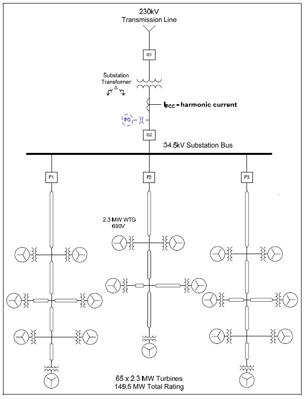
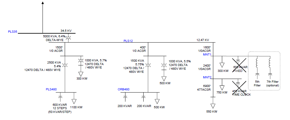
A wind plant substation IEEE Std. 519 harmonic measurement compliance case study was completed for the 34.5 kV wind plant substation shown in Figure 1.
Figure 1 – Illustration of Oneline Diagram for Harmonic Measurement Data Evaluation
The wind plant substation was supplied from a 230 kV transmission line and included a 180 MVA, 230/34.5/13.8 kV step-down transformer with a number of 34.5 kV collector circuits supplying 65 2.3 MW (690 V secondary) Type 4 full conversion wind turbine generators. The monitor was connected at the 34.5 kV transformer secondary, which was considered the point of common coupling (PCC).
The twenty-four day monitoring period was from November 16, 2009 through December 13, 2009. The power quality instrument used to complete the harmonic measurements was the Dranetz Power Xplorer PX5. The instrument samples voltages and currents at 256 points-per-cycle and follows the IEC 61000- 4-7 method for characterizing harmonic measurement data. This involves analysis of continuous 200msec samples and storing aggregated 10-minute minimum, average, and maximum trend data. The measurement and statistical harmonic analysis was completed using the PQView® program.
MEASUREMENT DATA ANALYSIS
Figure 2 shows the measured total plant power production during the twenty-four day monitoring period. Statistical analysis of the 61,901 individual steady-state power measurements yielded an average value of 27.081 MW, a maximum value of 144.872 MW, and a CP95 value of 129.203 MW. CP95 refers to the cumulative probability, 95th percentile of a value.
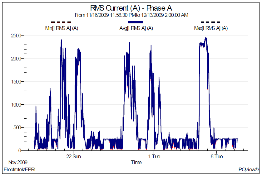
Figure 3 shows the measured total plant rms (Phase A) current trend. The corresponding phase current histogram is shown in Figure 4. The average value was 543 A, the maximum value was 2,449 A, and the CP95 value was 2,177 A (130 MVA). The CP95 value was used for the facility load current rating in the IEEE Std. 519 harmonic analysis.
Figure 2 – Measured Total Plant Power Production
Figure 3 – Measured Total Plant RMS Current Trend
Figure 4 – Measured Total Plant RMS Current Histogram
The IEEE Std. 519 harmonic voltage distortion limits for the wind plant installation are summarized in Table 1. The harmonic measurement data is evaluated on a statistical basis where the limit must be met 95% of the time (CP95).
Table 1 – IEEE Std. 519 Voltage Limits for the Wind Plant Substation
.
Figure 5 illustrates the corresponding measured total harmonic voltage distortion (THD) trend with an overlay of the IEEE Std. 519 total distortion (VTHD) limit of 5%. The average value was 2.18%, the maximum value was 4.23%, and the CP95 value was 4.09%. The measured voltage distortion was below the IEEE Std. 519 limit of 5%.
The harmonic current limits for the wind plant installation that are summarized in Table 2 are applied to the currents measured at the point of common coupling (PCC). The short-circuit ratio is not relevant for this application because the standard stipulates that power generation equipment must meet the most stringent limits. The limits are for the worst-case normal conditions lasting longer than one hour. For shorter periods, such as during start-ups or unusual operating conditions, the limits may be exceeded by 50%.
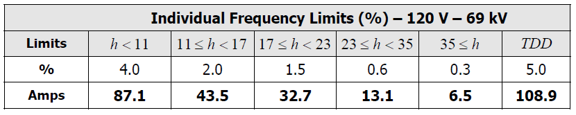
The standard provides the current limits as a percentage of IL, the maximum load current. The measured CP95 value of the load current was 2,177 A (refer to Figure 4). Table 3 shows the resulting current in both percent and amperes. Each of the lower order harmonic currents (h<11) must be no more than 4% of the maximum load current.
Table 2 – IEEE Std. 519 Current Limits for the Wind Plant Substation
.
Table 3 – Harmonic Current Limits at the PCC
.
Figure 5 – Measured Total Harmonic Voltage Distortion Trend
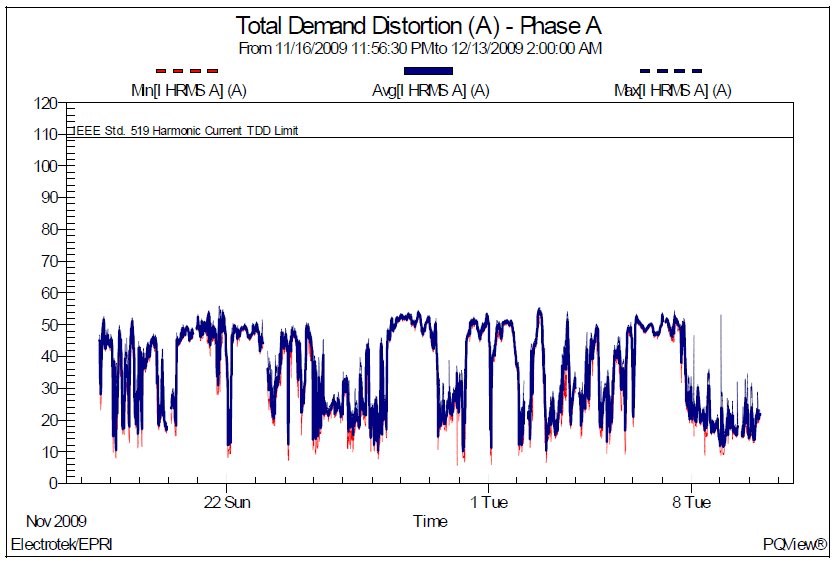
Figure 6 shows the measured total demand distortion (TDD) current trend with an overlay of the IEEE Std. 519 current distortion limit of 108.9 A. The average value was 35.75 A, the maximum value was 54.55 A, and the CP95 value was 51.65 A. The measured total demand current distortion was well below the IEEE Std. 519 limit of 5% (or 109.8 A).
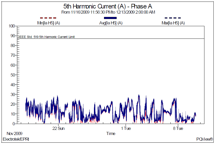
Figure 7 shows the measured 5th harmonic current distortion trend in amperes with an overlay of the IEEE Std. 519 current distortion limit of 87.1 A. The average value was 11.63 A, the maximum value was 28.92 A, and the CP95 value was 23.24 A. The measured 5th harmonic current distortion was below the IEEE Std. 519 limit of 4% (or 87.1 A).
Figure 8 shows the measured 7th harmonic current distortion trend in amperes with an overlay of the IEEE Std. 519 current distortion limit of 87.1 A. The average value was 30.91 A, the maximum value was 48.01 A, and the CP95 value was 43.80 A. The measured 7th harmonic current distortion was below the IEEE Std. 519 limit of 4% (or 87.1 A).
Figure 6 – Measured Total Current Demand Distortion Trend
Figure 7 – Measured 5th Harmonic Current Distortion Trend
Figure 8 – Measured 7th Harmonic Current Distortion Trend
Figure 9 shows the statistical summary of total harmonic voltage distortion (VTHD) and a number of the individual harmonics for the twenty-four day monitoring period. The analysis shows that the predominate harmonics for the measured substation bus voltages were the 5th, 7th, 11th, and 13th. The measured values were below the IEEE Std. 519 voltage distortion limits, which were 5% THD and 3% for any individual harmonic.
The statistical summary in Figure 9 corresponds to the voltage distortion measurement data previously shown in Figure 5 (voltage distortion trend). Statistical analysis of the measurement data yielded a CP05 of 0.75%, an average distortion of 2.18%, and CP95 value of 4.09%.
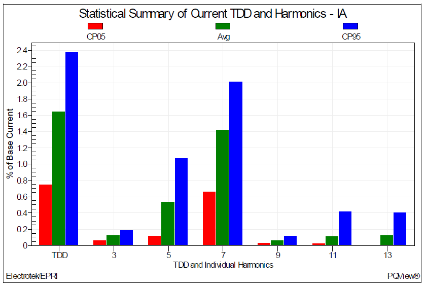
Figure 10 shows the corresponding statistical summary of total harmonic current distortion and a number of the individual harmonics for the twenty-four day monitoring period. The analysis shows that the predominate harmonics for the measured substation currents were the 5th, 7th, 11th, and 13th. The base current for the statistical summary was 2,177 A, which was the CP95 load current value previously used in the IEEE Std. 519 evaluation.
The statistical summary in Figure 10 corresponds to the harmonic current data previously shown in Figure 6 (current demand distortion trend). Statistical analysis yielded a CP05 value of 0.74%, an average current of 1.64%, and a CP95 value of 2.37%. Analysis of the measurement results showed that the harmonic currents did not exceed the IEEE Std. 519 TDD limits during the twenty-four day measurement period.
Figure 9 – Measured Statistical Summary of Voltage Distortion and Harmonics
Figure 10 – Measured Statistical Summary of Current Distortion and Harmonics
Figure 11 – Example of a Calculated Substation Current Waveform
Figure 12 shows the corresponding calculated voltage waveform created using the measured harmonic spectrum data. The fundamental frequency voltage was 20.395 kV, the rms voltage was 20.089 kV, and the voltage distortion was 3.33%.
Figure 12 – Example of a Calculated Substation Voltage Waveform
SUMMARY
This case study summarizes a wind plant substation IEEE Std. 519 harmonic measurement compliance analysis for a twenty-four day monitoring period. The wind plant substation supplied 65 2.3 MW wind turbine generators (149.5 MW total). The monitor was connected to the 34.5 kV transformer secondary winding, which was considered the point of common coupling (PCC) for the harmonic analysis.
The twenty-four day monitoring period was from November 16, 2009 through December 13, 2009. The power quality instrument used to complete the harmonic measurements was the Dranetz Power Xplorer PX5. The instrument samples voltages and currents at 256 points-per-cycle. The measurement and statistical harmonic analysis was completed using the PQView® program. Analysis of the measurement results showed that the harmonic voltages and currents did not exceed the respective IEEE Std. 519 limits during the twenty-four day measurement period.
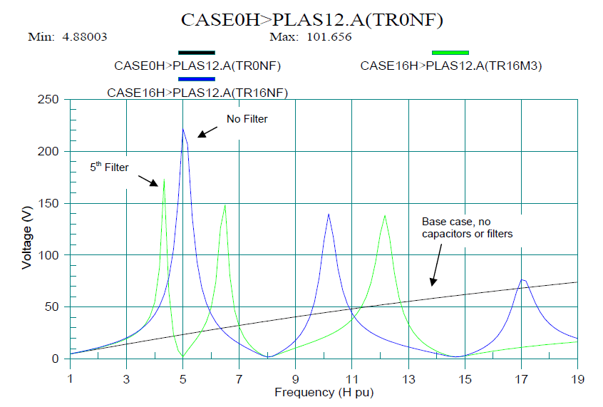
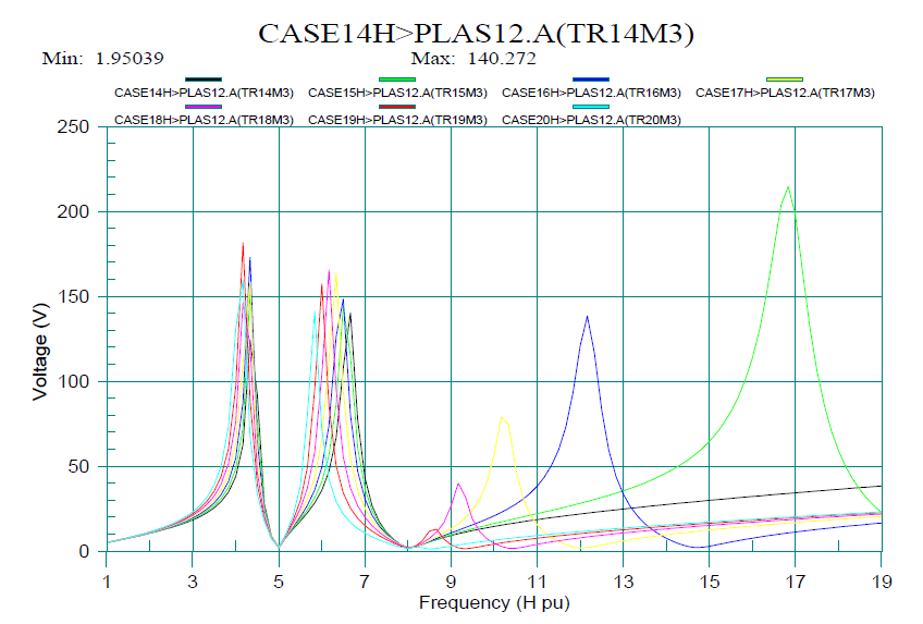
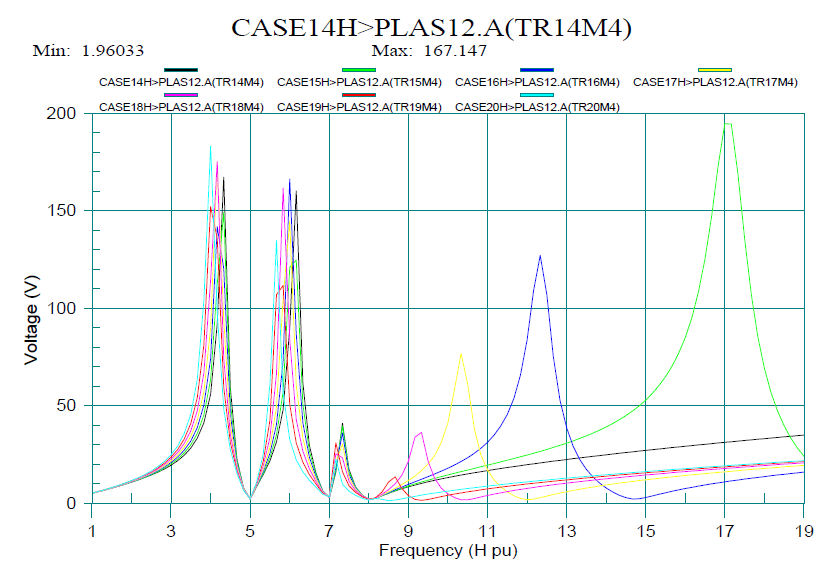
Mitigation alternatives for reducing harmonic distortion levels include methods for modifying the power system to reduce or eliminate the harmonic resonances that can cause very high current or voltage distortion levels. For example, a passive shunt harmonic filter may be added to the utility or customer system to divert the troublesome harmonic currents off the system and into the filter.
In addition, the rating of power factor correction capacitor banks may be changed to shift the harmonic resonance frequency and reduce the resulting voltage distortion levels. This is often one of the least expensive options for both utilities and their customers. Voltage regulation and power factor correction considerations should be evaluated before changing capacitor bank ratings.
REFERENCES
1. IEEE Recommended Practice for Monitoring Electric Power Quality,” IEEE Std. 1159-1995, IEEE, October 1995, ISBN: 1-55937-549-3. 2. IEEE Recommended Practices and Requirements for Harmonic Control in Electrical Power Systems, IEEE Std. 519-1992, IEEE, ISBN: 1-5593-7239-7.
Published by Adam SZELĄG, Tadeusz MACIOŁEK, Politechnika Warszawska, Instytut Maszyn Elektrycznych
Abstract. A 3 kV DC supply system, used on railways in Poland, since 1936, has power delivery capacity that allows reaching by trains a maximum speed of 250 km/h. Currently, the maximum trains service speed on Polish railway is 160 km/h, although speed record reached in 1994 was 250,1km.Therefore, it is worth modernising the system to increase power demand of trains with speeds 200-220 km/h, which will start service in year 2014. It requires application of proper methods to find compromise between the required effectiveness and the cost of the investments. The paper presents a system approach for analysis and synthesis of the 3 kV DC supply system used in a process of feasibility studies including a concept and a preliminary design.
Streszczenie. Stosowany na kolei w Polsce od 1936 r. system zasilania 3 kV DC pozwala na zasilanie pociągów osiągających maksymalne prędkości 250 km/h. Obecnie maksymalna prędkość pociągów na kolei w Polsce nie przekracza 160 km/h, aczkolwiek rekord prędkości osiągnięty w Polsce w 1994 r. wyniósł 250,1 km/h. Dlatego istotne jest, aby przeprowadzić modernizację zasilania trakcyjnego dla zapewnienia wymaganej energii dla pociągów o prędkościach 200-220 km/h, które pojawią się w 2014 r. Wymaga to zastosowania odpowiednich metod, aby uzyskać kompromis pomiędzy wymaganą efektywnością zasilania a kosztem inwestycji. W artykule przedstawione jest systemowe podejście do zagadnień analizy i syntezy stosowanych w procesie projektowania trakcyjnego układu zasilania, 3 kV DC w projektach koncepcyjnych i wstępnych dla celów studiów wykonalności (Modernizacja systemu zasilania trakcji elektrycznej 3 kV DC dla zwiększonego poboru energii pociągów o podwyższonej prędkości jazdy – zagadnienia analizy i syntezy)
Keywords: electric traction system, system analysis, modelling and simulation, power demand. Słowa kluczowe: system trakcji elektrycznej, analiza systemowa, modelowanie i symulacja, zapotrzebowanie na energię.
1. Introduction
Last year plans of construction of the so-called Y high speed railway line with maximum speed over 300 km/h with 2×25 kV 50 Hz power supply, postponed by the Polish Government, caused that focus has been put back at the 3 kV DC traction power supply system which has been used in Poland since 1936, but its power delivery capacity has not been reached. So it is worth analysing how it is possible to maximise usage of 3 kV DC system electrical energy delivery capacity for the increasing power demand and speed of trains over 200 km/h, even up to 250 km/h as it is applied in Italy at Dirretissima railway line [2]. A system analysis makes a useful tool for preliminary study and a concept design of an electrified transport system.
List of the used symbols:
ETS – electric traction system PSN – AC power supply network, TPSS – traction power supply system, ETV – electric traction vehicle, TS – traction substation
2. Electric transport system
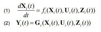
Elements of both the analysis and synthesis appear in the examination of issues and phenomena related to the functioning of the ETS. Therefore, methods with application of ETS subsystems models and their implementation, which allow the introduction of elements of the analysis – e.g., determination of a group of functional parameters of ETS power supply have been developed as [2, 4, 5, 6] substations load, catenary, voltage drops, efficiency, consumption and energy loss, etc. including: environmental conditions on the basis of the input parameters (characteristics) of the system. These include: distances between substations, types of rectifier units installed in the traction substations, catenary sections, the parameters of the electrical power engineering system. Other specified functional parameters are as follows: defined traffic, types of trains, locomotives, time-table with consideration of the technical limitations imposed on the ETS (technical criteria and reliability, the impact of ETS on the surrounding technical infrastructure and the environment – harmonics, voltage fluctuations, and stray currents). Dynamic model of the ETS system can be presented in the generalized manner in shape of a set of equations describing the respective subsystems [3,4,7] (Fig. 1):
.
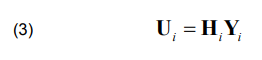
where: i=1,..,5 and structural equations:
.
where: Xi (t) – vector of state variable of ith subsystem, Yi (t) – output vector of ith subsystem, Ui (t) – control (input) vector of ith subsystem, Zi (t) – vector of disturbances of ith subsystem, Hi – structural matrix.
Dimensions of the matrix structural equations Hi depend on the number and types of ETVs moving along the railway line, the TPPS system and number of traction substations TS as well as their scheme of supply from the power system [1,4,6].
Elements of the analysis will also appear: when evaluating the possibility of maintenance of the existing supply system in the conditions of masses and train speed growth and the introduction of new locomotives with higher power,
– when determining the degree of utilisation of the existing devices installed in the supply system (the use of installed power), the load of wires and rectifier units of traction substations, energy transmission efficiency and power quality,
– when solving problems of compatibility of subsystems (electrical engineering power supply – traction supply system – traction vehicles – control and signalling systems) and electrical devices.
Elements of synthesis involve:
– selection and configuration of DC and AC power supply system (installed power, cross sections of wires, distances, supply voltage at AC side of PSN),
– selection of locomotives proper for a category of trains (mass and speed) for a specified line, based on the requirements for the functioning of ETS (traffic forecast) with consideration of limitations arising from the need of fulfilling the technical criteria (international and national standards and regulations) as well as reduction of distortions introduced by the ETS to the surrounding environment.
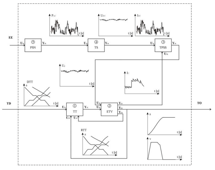
Fig. 1 Functional scheme of ETS system after decomposition into subsystems and presentation of exemplary time runs
Fig. 1 Functional scheme of ETS system after decomposition into subsystems and presentation of exemplary time runs (time axis scaled in seconds) of input and output values (TT – time-table; DTT – demanded time-table, RTT – actual (resulted) time-table ,TD – transport demand, TO – transport output; Ic- ETV’s current, Up-voltage in catenary, IDC – TS’s current, UDC – voltage at TS’s busbard, PAC – power taken by TS from PSN).
Due to the fact that the issue of synthesis usually cannot be solved explicitly, some additional criteria are being introduced:
– maximising utilisation of the installed devices power, – to provide reserve in a case of emergency, – possibility of overcoming speed reductions by trains with occurrence of traffic disturbances, – the system’s openness to changes in the traffic volume (the possibility of staging the development of ETS supply system with increase of energy demands from ETVs and maximising the use of existing infrastructure (optimal adaptation of ETS infrastructure for the transport forecast), – minimisation of energy transmission losses
Combining elements of the analysis and synthesis of ETS results in a complex problem, which will deal with the selection of ETS elements and determination of their parameters (rated power, overload, sections, etc.) and their mutual dependencies (e.g. voltage at the ETV’s collector functioning as dependence between TPSS and ETV or changes of traction substation load giving an influence on PSN, similarly changes of voltage in the PSN have the impact on the operation of traction substation).This refers to the exploited (manufactured) devices as well as to defining the requirements for implementation of new measures due to the defined demand for transport (traffic forecast- traffic flow TD and the resulting demand for electrical energy EE (Fig. 1), functional requirements – quality and reliability of supply, and the interaction between different ETS’s subsystems as well as between ETS and the environment.
In developing new methods for analysis and system design with respect to exploited lines as well as newly constructed, it must be assumed that in principle one is dealing with a complex problem, which combines elements of both synthesis and analysis. All the assumptions made at the stage of analysis of functioning conditions of the existing ETS as well as design of new lines or improvement actions e.g.:
-aiming at: – rationalisation of energy consumption or effective energy consumption (improvement of its usage), -introduction of a new stock or changes in traffic, -introduction of new control systems
must take into account existing state of ETS, its parameters and functional requirements. Therefore, all the actions (as forecasts) oriented towards improvements (as increasing efficiency) should result from the analysis of the existing state and then on the basis of results of such an analysis, by application of assumed technical criteria (e.g. rationalising the energy consumption, maintaining the distortion level at permissible limits) lead to changes (choice of modernisation option-elements of synthesis), which will improve or even enable the operation of a system.
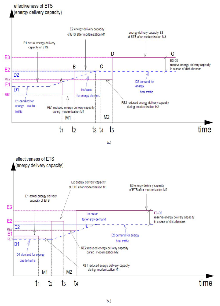
Fig. 2a,b Graphs showing exemplary changes of energy delivery capacity of ETS
Fig. 2a,b Graphs showing exemplary changes of energy delivery capacity of ETS (obtained by modernisation stages M1 and M2 of the existing TPSS of the ETS’s) versus time due to increase of demand for energy (blue broken lines) by transport means. Please observe reduction of the energy delivery capacity (RE1<E1, RE2<E2) of TPS during the modernisation processes, which will force reduction of traffic (RE1<D1 during M1; RE2<D2 during M2).b.) modernisation undertaken early enough with lower reduction of capacity (t1 in Fig.2b < t1 in Fig. 2a and RE1 in Fig 2a < RE1 in Fig. 2b) to get the required energy delivery capacity E1 to E3 high enough above the energy demand D1 before its increase to D2 due to traffic increase.
3. Application of a system analysis in the ETS.
The analysis of the ETS system as a research method is used when the situation occurs, in which the state of the system is currently or will in future be unsatisfactory, and it can be anticipated that the actions (modernisation) may improve the situation significantly (Fig. 2). After the analysis we obtain the system description of the situation, as well as courses of action, which will produce positive effects.
The results of such an analysis may be used by policy ma-kers to choose the most advantageous solution due to the certain criteria. In addition, a system analysis allows for the justification of purpose of the selected variant against pressures from the side of interest groups and against the wrong interpretation of the phenomena. It is a crucial factor because the results may have significant influence on the range and cost of the infrastructure modernisation.
The results obtained from the analysis of the system also allow reference to the unexpected events or disturbances in the functioning of the system.
In Fig 2a there is shown time-varying demand for energy used by moving ETVs and effectiveness (energy delivery capacity) of TPSS. Application of a system analysis to ETS allows assessing effectiveness of ETS when increase of demand for energy due to changes in traffic is expected (from D1 to D2). When the effectiveness E1 (energy delivery capacity of the ETS) is becoming close to the energy demand (time point t1) implementation of improvement processes – modernisation is to be started – point A (period of modernisation M1 between t1 and t2 – points A-B, period t4–t5, M2-points C-D). Effectiveness of ETS during modernisations M1 and M2 energy delivery capacity is reduced (for modernisation period M1 – effectiveness RE1 between points B-C and RE2 during M2 – between points C-D) as well as change of demanded energy delivery due to change of traffic (increase from D1 to D2).
As example we could assume the existing two-track ETS with 3 kV DC supply and a bilateral supply scheme with traction cabin TC in the mid-points between neighbouring traction substations TS – fig.3a. As a measure to enhance the energy delivery capacity of ETS, after application of the system analysis, the improvement of ETS to by process of modernisation M1 is undertaken. It may be, for instance, construction of new traction substations in positions of traction cabins (Fig. 3b). This will enhance the effectiveness of the ETS above the increasing demand D (period t2-t4). And again, when as a result of the system analysis it was predicted, that additional modernisation M2 of the ETS is required; a construction of traction cabins TC between traction substations may be done (Fig. 3c). It could slightly improve the effectiveness of the 3 kV DC ETS above the energy demand level (Fig. 2a).
In order to maintain the energy capacity proper for energy delivery even during the modernisation process it is required to start it before the demand will be increased and assure that during the process of the modernisation power capacity will be high enough (Fig. 2b).
System analysis of the assumptions is not conducted for a particular decision maker, but in most cases, the decision maker orders such an analysis so to obtain as much information for undertaking a decision as it is possible. The result should include all the possible consequences of any line of conduct. The analyst should clearly establish the expectations of the decision maker, outline possible alternatives, consider consequences of each option, and then arrange them accordingly to selected criteria. In practice, decisions are not always proceed with accordance to such a scheme, but if it deviates from such a scheme, it occurs only to a minor extent. System analysis related to ETS should also be based on this scheme. To achieve the objectives (such as reduction of electricity consumption by railway vehicles, an increase in average driving speed, reduction of the amount of emergency on the railways, etc.) set by the decision maker, one creates different types of solution variants (e.g. reconstruction of the supplying substation, changes in the profile line, change of traffic, etc.).
To explore the various options, models that can be used to assess the effects of the variant or the cost of its implementation are created. Specifically the cost, effectiveness and feasibility of the option are the important factors [8,9,10].
For different variants may emerge the need to use different models. The use of different models may be necessary to prioritise the options for different purposes. The analysis should end with a rearrangement of variants and be presented to the decision maker together with the effects of each variant. In the majority of issues related to ETS, factors affecting the results are considerable and their mutual relations rather complex. Such a situation causes that intuitive approach will often lead to erroneous and costly solutions. Application of coupled models, in mathematical terms, is necessary for the appropriate formulation of description of ETS functioning and analysis of its operation in different variants of solutions.
4. Procedure for an ETS system analysis
Finding the solution for the improvement of the existing state or choosing the best target variant requires knowledge and clarification, as careful as possible, the aims of decision maker. On such account, one should determine options to achieve these objectives. A further step is to rank the possible options. Implementation of such a procedure will generate further questions. In order to determine the possible variants to achieve, it is not sufficient to be aware of goals, but also to know the area in which the decision maker has the freedom of action. For the ranking or comparison of variants, one may need to anticipate the consequences that will result from implementation of each variant (also those that do not link directly to the realisation of goals). Determination of the consequences of each option requires the use of an appropriate cause-effect model, which will allow the decision maker to indicate the consequences of the choice of a particular variant. Such a model should also take into account the uncertainty of future conditions, such as changes of external conditions other than those assumed in the analysis.
In extreme cases, the variants may differ considerably among themselves, because in principle the implementation of a goal is possible through different ways of proceeding. In such situation it may be necessary to apply various models for different groups of variants. It can be also justified to use models of different degree of specificity depending on the analysis of a state. Main steps of system analysis include:
Main steps of system analysis include:
a) formulation of a problem taking into account assumed goals, b.) defining and working out the variants, c.) selection of variants on the basis of constraints, d.) development of forecasted situations , e.) construction of models, f.) application of models for foreseeing effects, g.) comparison and ranking of the obtained variants.
Analysis of the results or a preliminary version of final results may lead to a modification of the previous assumptions.
Typical interactive loops that occur are following:
a) improvement options loops, in which occur a modification of parameters in various options for attainment options preferably pursuing the goals; in some cases this process can be implemented by means of optimisation procedures;
b) problem formulation loops, in which on the basis of the results of an analysis the modification of goals is performed;
c) analysis of restrictions loops, in which it is, evaluated how, changes of restrictions influence the degree of goal accomplishment;
d) loops of tuning (adjusting) models, in which particular elements of models or complete models are either simplified, for the purpose of attaining less specific but more certain decisions, or detailed so as to emphasis the more important characteristics of variants.
Furthermore, if one considers that the process of implementation of the selected option may be too long, it must be accounted that the actual conditions, in which the variant is carried out, may differ from those assumed at the stage of analysis. In such case, refinement of options for changeable conditions – during the process of implementtation and if it is possible – correction of a project, can be applied. At each stage of the system analysis contacts of an analyst with a decision maker (or contracting the project) are of high importance. The original formulation of the problem is never exhaustive and does not include the whole spectrum of situations. The results of the analysis have an impact only on the initial view regarding the solutions. Both the goals and the restrictions can be modified during the process of analysis, and the considered time horizons may be a subject to changes.
5. Formulation the problem
Formulation of the problem includes:
-identification of the tasks to be solved, -determination of the scope of the solutions for these tasks, -clarification of the objectives, -determination of what devices and to what extent may the proposed solutions affect, -initial proposal for the approach to the analysis
Stage of formulation of the problem should give an initial indication of the purpose and if possible, identify the objectives in a quantitative manner, identify preliminary alternatives for analysis, lead to the definition of restrictions and a determination of the expected effects. Formulation of the problem is therefore a very important step, because its correct implementation allows the determination of whether the problem is artificial or trivial, and also provides a framework in which one can move through the later stages of analysis. Difficulties encountered during the formulation of the problem:
a) the interrelations of the subsystems – changes in one subsystem affect other subsystems and assessment of impacts of the performed actions in interrelated objectives, constraints and consequences for the individual subsystems is difficult to conduct;
b) the difficulty of determining the goals, without the approximate values of the effects, which will result from the introduction of options, it is difficult to define precisely the objectives;
c.) lack of clear criteria for selection, the decision maker preferences may be difficult to define, and they may change within time.
Therefore, this step should be the object of application of a system analysis.
The goal, which designates the decision maker (e.g. ETS operator) to be achieved, can be declared in a more or less detailed manner (“energy efficiency”), and can also be defined in quantitative terms (e.g. “to reduce traction energy consumption by 10%”, “to reduce transmission losses on the DC network by 20%“,” to reduce demanded peak power by 5%”, etc.).
The decision maker may seek to achieve different objectives. Sometimes the decision maker gives only the most important goals while an analyst (project contractor) must be aware of the possibility of unspecified purposes or purposes given in the form of restrictions. Usually, while solving issues the decision maker determines several goals, among which there are competing goals, that is, that the improvement in one of these objectives leads to deterioration in other aspects (e.g. efforts to reduce losses increase requirements for installed power, which in turn increases the idle losses of transformers). In this case, one should use the following approach:
a) determine the sequence of objectives; b) identify the most important goal; c) all the objectives should be transformed into restrictions and one should seek solutions possible to be implemented, d) establish evaluative system by ranking goals.
With the overall goal of rationalization of energy consumption on the railways, the decision maker may also have other objectives: to increase the average speed of selected categories of trains, improve comfort, increase safety on the railway lines, improve punctuality, and reduce failure rates. Some of these goals are competitive, while other can be achieved in the same ways of implementation (e.g., by reducing gradient of track energy consumption for traction purposes is reduced and also the ride comfort is increased).
To evaluate the analysed options one should have a measure value of the effects, which are brought by each of variant. Some of the results are easy to estimate numerically, while other – the more abstract – are not. The efficiency of the power system, the maximum power demand or the global energy consumption on the railway line can be written in the form of numbers, and parameters such as: ride comfort requires preparation of tools to describe this rather abstract and ambiguous concept (e.g., through the application of special tariffs for journeys with a high standard of the offered transport service).To compare the options it is not enough to describe the quantitative results obtained in each of them. One should use the criteria enabling the proper ranking of the options.
However, since there are often not universal, objective criteria for sorting options, so in each individual case, such criteria should be established, mainly on the account of the value scaled by the decision maker. Using these criteria, one can also take into consideration the opinion of external factors, which will be influenced by the effects resulting from the implementation of a given variant.
During the formulation of the problem one must also specify the area of restrictions. They may arise from the physical properties of the analysed systems (e.g. power capacity of the supply), but also from the accepted standards (e.g. level of voltage in catenary) or imposed require-mints (e.g. density of traffic or maximum power of trains). These variants, which are not prohibited by the restrictions (do not meet the criteria) are called permissible or attainable.
Some restrictions are permanent and can never be exceeded (e.g. cross-section of catenary due to applied type of support structures), some may change over time (as increase of power capacity due to investments in power supply system) and due to the change in requirements (e.g. change in assumed time-table and type of locomotives), and some are imposed by the top-down decisions. For the restrictions that could be alleviated (e.g. density of traffic), the analyst should carry out the consideration of how such alleviation would affect the achievement of the objectives (e.g. lower density of traffic may require bigger mass of trains), and what would be costs of such restrictions reduction.
In the analysis of the phenomena occurring in the ETS, the restrictions may include: technical parameters of the vehicles and the supply system, speed limits on the sections of the line, minimum voltage at the pantographs of trains. A restriction may also constitute a lack of opportunity of location traction substations at the specific point of the ETS or change in the type of catenary or lack of possibility to implement a freely shaped time-table.
6. Creation and selection of variants
Variants taken into consideration during a system analysis can vary considerably. They do not have to constitute their substitutes and do not have to assure the performance of the same functions.
The initial stage of variants’ creation should com-prise all the possible ways of proceeding, so giving at least partial chances for the accomplishment of objectives. In the set of analysed variants, usually the so called „zero” (do nothing) option is included. This variant is mainly used for comparative purposes (as a ‘reference option’).
Usually during the analysis of the selected variants occur new variants, which at the beginning have not been known to the both analyst and decision maker.
For the purpose of an exemplary task of rationalisation of energy consumption of ETS, a range of creation of diverse variants may be wide. This may include: changes in time schedule, rolling stock replacement, reconstruction of the supply system or even the reconstruction of the whole line (e.g. alleviation of the route profile). Each of the variants can to various extent influence the achievement of a goal and costs of their implementation are also diverse. For these or even other methods aiming at reduction of energy consumption on railway lines, it is possible to create a huge amount of options to be considered. Since the number of variants that have been generated at the beginning of the analysis may be large, they should undergo a pre-selection. Many variants can be rejected at the outset, because they do not comply with the restrictions. This can be observed using very simplified models, which give approximate results. In this manner, variants that are worse than others, at least in one aspect and in other aspects no better than remaining options can be eliminated.
Further stages should be conducted on detailed models with respect to quantitative parameters. The last stage of the ETS analysis should, in a possibly full and accurate manner, describe the processes occurring after the implementation of various options, so as the decision maker knows the extent to which each of they pursue goals and what are the further effects. At this stage one can enter the optimisation procedures. Multi-criteria optimising algorithm can be applied with usage of a scalarization approach and a goal function or penalty function defined for the optimisation algorithm.
Since the parameters, on which we have the influence, usually do not change continuously (e.g. it is impossible to select smoothly the cross-section of catenary, power supply and transformers parameters, numbers and parameters of rectifier units) the number of possible variants is significantly narrowed and the search for global analytical solution is not justified. In that case it is possible to use any of the random algorithms.
To anticipate the effects of the implementation of different options it is necessary to use system models. It is most preferable when models are formalized and written in a mathematical form. On the basis of such models one can develop the computer implementation of models in order to conduct the simulation tests.
Analysed variants may differ among sets of data assumed. Set of data regarding the state of environment can be taken as constant (when these parameters are strictly defined) or variable (when there is uncertainty about these parameters). In the latter case, it is recommended to conduct a sensitivity analysis of the effects of variants on the changes of the environment state so as to assess the uncertainty of achieving the objectives for each of the variants.
An exemplary division of the electrified railway line parameters at the design stage of this line can be a division into: independent (top-down set)-the size of transport and into dependent (those we have an influence on) -technical parameters of a supply system (to meet the technical criteria for the implementation of the given traffic flow) or organisation of train schedules at a given transport demand.
Obviously, for the proper construction of models it is not enough to know the general form of mathematical equations describing the analysed system as they should be verified and tuned to the actual conditions.
7. Range of applications of modelling and simulation techniques in the ETS
The range of applications of computerised techniques to area of ETS may be enlisted to one of the following groups, due to:
a.) CAD (computer-aided design) during planning stage of the ETS, its subsystems and components,
b.) analysis strategy of operation of the ETS – design of timetables, traffic control, centralised and decentralised control and management of the ETS,
c.)for design of operational service and control system, operational, control, surveillance and decision supporting systems-e.g. methods of optimisation of ETVs motion and operation of TPSS with regard to energy consumption,
d.) the use of specialised software for ETS simulations during steady and dynamic states – for the analyses of supply system loads, main circuits of electric traction vehicles, control and signalisation systems, mutual interactions between subsystems (ETVs-TPSS; high power circuits-track circuits, etc.) and electromagnetic fields- in the range of distorting inference of the ETS and its influence on the surrounding environment and technical infrastructure.
Due to the complexity and multi-aspect nature of phenomena as well as available technical devices, methods of the analysis and design are oriented at considering certain types of problems as:
a.) energy problems (delivered power, energy consumption, energy losses etc.), regarding the phenomena occurring at electrical steady states in AC and DC circuits; for the analysis of such problems it is sufficient to use static models considering the average and equivalent values, such as peak, average and equivalent power and currents of load or stray currents flow ,
b.) electromechanical aspects – concerning both motion and power collection by the ETVs as well as resultant TPSS load, which is associated with energy problems. The mutual interaction of TPSS and ETVs should be taken into account, due to the influence of voltage in a catenary on motiontraction parameters of the ETVs (dependence of voltage in catenary on the ETV’s traction characteristics). The derived models should incorporate dynamics of load changes of TPSS and ETVs motion. Therefore, they have nature of dynamic models (with regard to phenomena of ETVs electromechanical constants values in range of tens of seconds), in which during the analysis of state of the ETS system at the given time step, the ETS state at the previous step is taken into account.
c.) electromagnetic problems and transient states– occurring in much shorter time than the phenomena of electromechanical type (b), which requires the development of models for analysis of the fast-changing phenomena (such as short circuit, overvoltage, transients) and analysis time runs for the content of the component variables (including harmonics) and the resulting ability to assess interferences introduced by ETS to the surrounding technical infrastructure.
d.) problems with traffic and transport management (for set volume of transport, traffic structure, types, masses, train speed). For each group of problems a)-d.) equations take a specific form, thus in the following project, emphasis was put on the proper selection of models for the problem under consideration.
Proper functioning of the ETS is conditioned by, apart from fulfilment of functional requirements (realisation of transport tasks), an attempt to redeem technical requirements and constraints regarding e.g. capacity of energy transmission by TPSS to ETV (groups a. and b.), but also the proper cooperation with both surrounding technical infrastructure and environment.
In case of negative assessment in the analysis with application of models from group c), ETS given variant, even if it turns out to be optimal because of other criteria (e.g. energy consumption) should be rejected as not meeting the basic technical conditions. Solving the subproblems of the system operation may be impaired due to the interferences Z (Fig.1.) occurring in any subsystem (as disruption of traffic organisation, power supply system breakdown, short circuit in the catenary, damage to rolling stock, unplanned slowdown etc.). Therefore, the main task is to maintain the proper functioning of the system even under conditions of interference and the possibility of transition to a state of normal operation (e.g. traffic congestion release, catch up the delay) at the lowest cost (power consumption).
Fig. 3 Stages of modernisation the existing of the ETS (a.), after M1 modernisation (b.) and after next one M2 (c.)
To ensure the functioning of the system in conditions of distortions it is necessary to introduce certain breakdown restrictions in the description of a system operation. These restrictions will depend on the type of corrective actions (improvements) to be taken in case of failure. This approach sometimes requires an algorithm with conditional instructions, the automatic decision-making methodology performed by the simulation program (elements of artificial intelligence) or by the operator from the outside (stop of the program and the need to take a decision on the selection of an algorithm of further simulation or changes in assumptions).
In situation when in the program there are various algorithms of proceeding and choice of solutions, which support the work of operator, in case of a need for intervention, one can speak about elements of an expert system (decision-making support). Such a comprehensive approach to problem analysis and design ETS – selection of technical solutions required to deliver the overarching goal: supply of adequate quantities of electricity of a certain quality parameters to ETV, performing the set transport constitutes a fundamental assumption with respect to the formulation and the required structure of the ETS model system and its subsystems.
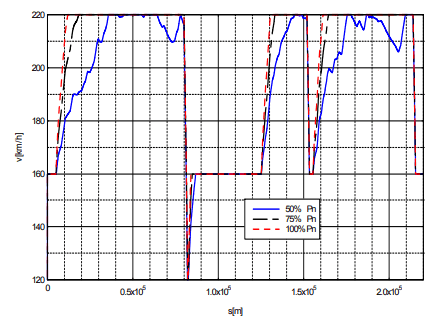
Fig. 4 Results of simulations of movement of a 426 t train set with influence of voltage on a rated power Pn availability (50%; 75%; 100%). (Pn=5,5 MW).
Conclusions
The necessity of development and modification of classical methods, established long time ago and used in the analysis and design of ETS ensures from the fact that there was, especially in the country, synthesis approach to issues that takes into account not only the complexity of electrical and mechanical phenomena occurring in the STE but also specificity resulting from local conditions in Poland (such as significantly lower than in other countries which use the 3kV DC power supply options for the ETV because of the large voltage drop in the supply system) and the interaction between the subsystems. An important feature is a combination of a simulation package with blocks of postprocessors analysis, which allows the support of system functioning evaluation (the comparison of set up and executed timetables, meeting the technical criteria, efficiency, energy consumption per unit, introduced distortions, etc). Due to the significance of such issues as compatibility of electrical subsystems and environmental impact as well as energy-electromechanical orientation of developed simulation software, results obtained with the help of programs for ETV’s motion simulation can be supplemented with the use of simulations developed in the course of these project models of ETS subsystems. They are designed for analysis of issues as: interference from higher harmonics, voltage fluctuations or transients in power supply or disturbance emission. This allows for conduction of detailed simulation studies on selected, identified as critical elements for the functioning of ETS conditions of cooperation of selected subsystems in transient states (short-circuit, overvoltages in TPSS and the possible to occur interferences between subsystems TPSSETV and impacts on traffic control circuits. Voltage at the pantograph of the locomotive influences the power developed by the traction drive according to its traction characteristic. It is defined by EN 50-338 standard. In order to put into service with maximum speed above 200 km/h on CMK railway line train sets with nominal power up and above to 6 MW it is required to enhance its traction power supply system. During the performed studies [7] a set of analyses has been performed for different time-tables and variants of operation of the power supply system. The main aim was to find the effective solution to modernise the power supply system to the stage allowing obtaining the required speed with utilisation of the installed on board of vehicles power.
In Fig. 4 there are presented results of simulation of a 426 t train-set with maximum speed of 220 km/h – a theoretical run on a section of track with speed restrictions. – speed “v” versus position of the train. It may be observed influence of the available power (100%, 75% and 50% of nominal power Pn = 5,5 MW) on traction parameters of the train – specifically opportunity of acceleration (as route sections 10000 to 30000 or 165000 m) in a region of higher speeds (above 180 km/h) or maintaining maximum speed, when gradient is increasing (as sections 65000 to 75000 or 195000 to 205000 m). A system analysis with application of the described in the paper method has been worked-out in order to receive the effective power supply system for a defined traffic forecast. It appeared, as a result of the analysis, that it is required to construct additional traction substations TS in locations of traction cabins TC (migration from a scheme 3 a. to 3 b.) in areas, where the power capacity of the supply 3 kV DC system and trains power demand by trains were not balanced with high enough level of voltage in catenary
REFERENCES
[1] Arrillaga J., Smith B. – AC-DC Power System Analysis. IEE London, 1998 [2] Capasso A., Buffarini G.G., Morelli V., Lamedica R. – Supply system characteristics and harmonic penetration studies of the new high speed FS railway line Milan-Rome-Naples. IEE Int. Conference on Main Line Railway Electrification, York (UK), 1989 [3.] Kaczorek T. Teoria wielowymiarowych układów dynamicznych liniowych. WNT, W-wa, 1983. [4.] Lewandowski M. -A Analiza zjawisk elektromechanicznych w szynowym pojeździe trakcyjnym z uwzględnieniem zmian współczynnika przyczepności kół napędowych Zeszyt “Elektryka” nr 139, OWPW, 2009 [5]. Mincardi R., Savio S., Sciutto G. – Models and tools for simulation and analysis of metrorail transit systems. COMPRAIL’94- Computers in Railways – Fourth Int. Conference on Computer Aided Design, Manufacture and Operation in the Railway and Other Mass Transit Systems, Rome, 7-9 September, 1994 [6] Szeląg A., Mierzejewski L. – Ground transportation systems. (in: The Encyclopedia of Electrical and Electronic Engineering. Volume: Suplement I, John Wiley &Sons, Inc., NY, USA ,2000) [7] Szeląg A.- Zagadnienia analizy i projektowania systemu trakcji elektrycznej prądu stałego z zastosowaniem technik modelowania i symulacji. Prace Naukowe PW, Seria ELEKTRYKA, s. 178, z. 123, 2002 [7] Szeląg A., Maciołek T., Drążek Z., Patoka M., Urban A., Załuska Z. at all– Ekspertyza dotycząca układu zasilania sieci trakcyjnej linii CMK, praca na zlecenie PKP Energetyka S.A., 2012 (not published) [8]. PHARE Project no PL 9309/0203 „Power Supply Study for E-20 Railway Line Kunowice-Warsaw section” (ITALFERR, Włochy, Politechnika Warszawska) (not published) [9] EC Project UserGroup and InfoBank to support rail interoperability. GMA2-2000 32015 Projekt Badawczy V-tego Ramowego Programu Unii Europejskiej. 2002-2003 [10] Projekt EUROPEAID/112846/D/SV/SI, Pomoc Techni-czna we wdrożeniu systemu GSM-R,ERTMS/ETCS i zdalnego sterowania urządzeniami stałymi systemu trakcji elektrycznej sieci kolejowej Kolei Słoweńskich. (Kolprojekt, Holland Railconsult, Austrokonsult, Omegaconsult), 2003 (not published)
dr hab. inż. Adam Szeląg, doc. dr inż. Tadeusz Maciołek Politechnika Warszawska, Instytut Maszyn Elektrycznych, Plac Politechniki 1, 00-661 Warszawa, E-mail Adam.Szelag@ee.pw.edu.pl; Tadeusz.Maciolek@ee.pw.edu.pl
Source & Publisher Item Identifier: PRZEGLĄD ELEKTROTECHNICZNY, ISSN 0033-2097, R. 89 NR 3a/2013
Published by Mateusz DUTKA1, Bogusław ŚWIĄTEK1, AGH University of Science and Technology, Department of Power Electronics and Energy Control Systems (1)
Abstract. This paper describes relevant issues of the energy prediction from onshore wind farms. The use of a neural network to forecast wind power production and its resistance to changing seasons is examined. Different structures of neural networks are presented with a comparison of their forecasts accuracy.
Streszczenie. Artykuł opisuje możliwości prognozowania produkcji energii w śródlądowych farmach wiatrowych. Analizie poddano możliwość predykcji z wykorzystaniem sztucznych sieci neuronowych uwzględniających wpływ sezonowości. W artykule zaproponowano różne struktury sieci neuronowych oraz porównano ich skuteczność.(Wpływ sezonowości na pracę i prognozowanie produkcji energii elektrycznej śródlądowej farmy wiatrowej).
Keywords: wind power forecasting, impact of seasonality, BP-neural network, efficiency, energy balancing Słowa kluczowe: prognozy farmy wiatrowe, wpływ sezonowości, sieci neuronowe, efektywność, stabilizacja systemu energetycznego
Introduction
In many areas of central Europe, in particular in Poland, a rapid development of renewable energy is more than visible. The growing significance of renewable sources entails the necessity of combining customers into groups within a region or a commune and the use of appropriate energy storage [1]. The electricity balance could be managed on the commodity exchange. In this case, the creeping trend model can be useful [2]. The model allows forecasting prices in a 24-hour horizon. The proper preparation of data for further analysis is associated with their normalization [3]. Among all renewables, the wind and the solar energy have been the fastest growing ones. Although in Poland, the construction of the first offshore wind farm is still being discussed, there is a tendency in the construction of inland farms with a growing number of turbines and their total installed capacity. The increasing number of wind farms located in Poland forces investors to locate farms in areas characterized by more difficult weather conditions. Farms are built on smaller areas or near existing farms which introduces interaction between turbines. In particular, when it comes to seasonal variability of wind and its turbulence. In order to increase the accuracy of prediction of wind speed [4], energy production [5] [6] in wind farms, various types of statistical and physical models have been successfully developed [7] [8].
This paper examines three neural network models for energy production forecasts from onshore wind farms, based on the use of artificial neural networks. The main advantage of this method is a relatively short time needed to obtain a good accuracy forecast [3]. The method uses models which were built on the basis of data from the farm and takes into account the impact of seasonality.
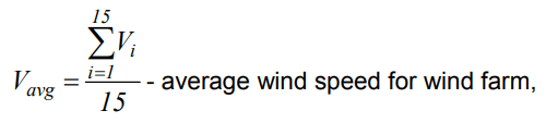
Analyzed farm are consists of 15 wind turbines manufactured by Enercon GmbH type E 70 – E4 with rated power 2 MW. The average annual energy production is over 50 000 MWh. The wind park with a total installed capacity 30 MW is located on a hill with the area of 270 ha. The relative height of the plateau is about 150–170 m (350 – 470 m m.a.s.l.). The wind turbines are located approximately 450 m away from one another. Installation height of a generator hub is 85 m, rotor diameter is 71 m, swept area: 3959 m2 . This study uses data from years 2012-2014 (full three years) consisting more than 150,000 vectors (10-minute intervals) registered form the SCADA. The study was performed with the use of following parameters: wind speed, wind direction and the power generated by each of the turbines and the total power generated by the wind farm.
The seasonality impact on work wind farm
The power generated by wind turbines depends significantly on wind speed, but also on the density of air. During the year, weather conditions change periodically. Slight changes in wind speed, temperature, pressure and humidity can evoke a significant change in power generated by the wind turbine. The impact of seasons on wind speed and direction and the volume of production was analyzed.
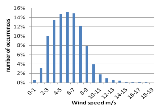
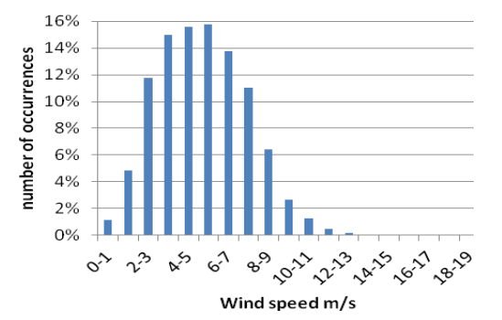
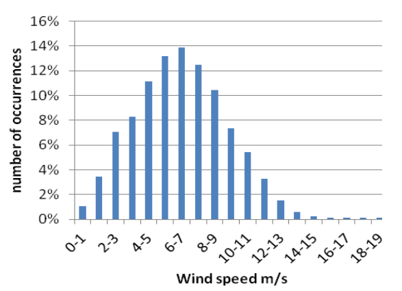
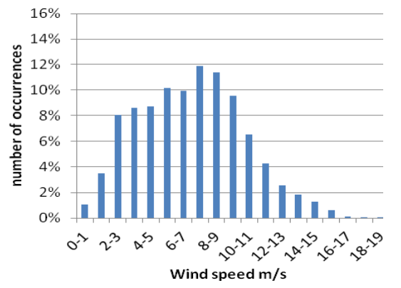
The following Fig.1-4 show the number of wind speed sets with a resolution of 1 m/s recorded by the turbine. Figures summarize operating conditions of a wind farm as the number of registered occurrences of wind speed in the whole analyzed seasons.
Fig.1. Percentage of the number of occurrences depending on wind speed – spring
Fig.2. Percentage of the number of occurrences depending on wind speed – summer
Fig.3. Percentage of the number of occurrences depending on wind speed – autumn
Fig.4. Percentage of the number of occurrences depending on wind speed – winter
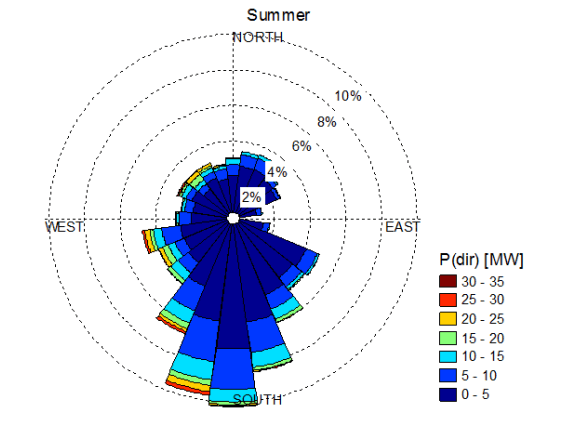
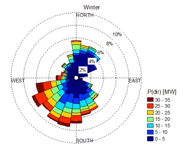
Analyzing the Figures 1-4 differences in wind strength between seasons are noticeable. During the spring and summer wind mostly blows at a speed of 5-6 m/s, during the autumn it increases to 6-7 m/s, while in the winter it reaches even 7-8 m/s. The biggest differences are visible between summer and winter. Although the speed changes to a small extent, it has a significant impact on the quantity of produced energy. Figures 5-6 summarize the frequency and volume of energy depending on the wind direction changing in increments of 15 degrees for two of the most different seasons (summer and winter) when the highest and lowest power outputs are recorded. The distribution of wind directions for both seasons is similar, most of the time the wind blows from the south and south-west.
Fig.5. The frequency and the amount of power of a wind farm depending on wind direction – summer
Fig.6. The frequency and the amount of power of a wind farm depending on wind direction – winter
Fig. 5 and Fig. 6 show two of the most different seasons of the year in which the highest and lowest power outputs are recorded. The distribution of wind directions for both seasons is similar, most of the time the wind was blowing from the south and south-west.
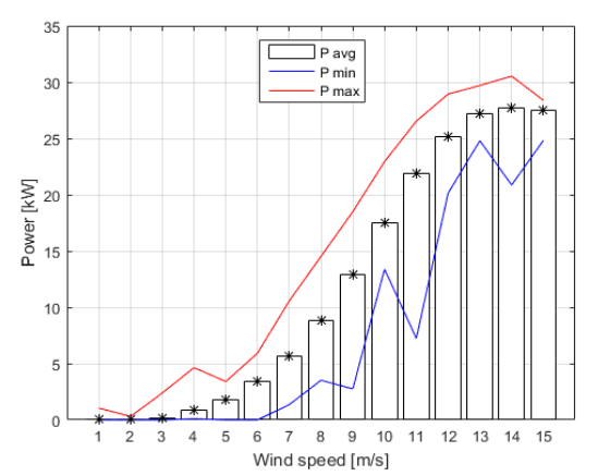
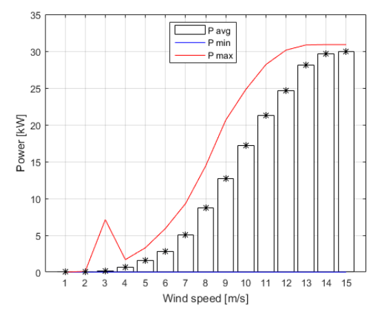
The amount of energy production is strongly dependent on the variable wind speed. Figure Fig. 7 and Fig. 8 below are showing the dependence of power on wind speed for summer and winter.
Fig.7. Power variation depending on wind speed – summer
Fig.8. Power variation depending on wind speed – winter
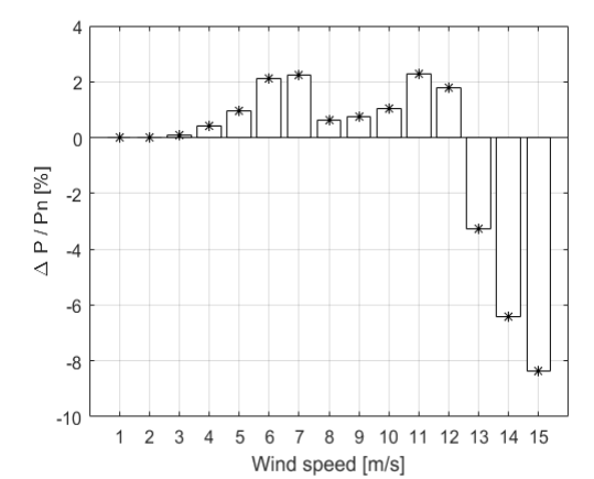
Fig.9. Difference in power variation depending on wind speed for summer and winter
Fig.7 and Fig.8 shows that different average production volumes for the same wind speeds are visible.
As can be seen in Fig. 9 in winter production is on average even higher by 8% for the same wind speed ranges compared to the summer period for wind speeds of 12-15 m/s,. For a smaller wind speed 3-12 m/s the opposite situation is visible.
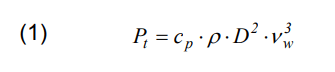
Wind power can be described by dependence:
.
where: Pt– turbine power [W], cp – efficiency, D – diameter of the rotor, ρ – air density.
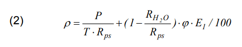
The wet air density can be expressed by the formula:
.
where: ρ – density of air [kg/m3], P – pressure [Pa], T – temperature [K], φ – relative humidity [%], φ=e/E2·100 [%], e – current vapor pressure [Pa], e = E2·φ/100, E1 – maximum vapor pressure [kg/m3], Rps– individual dry gas constant air [J/kg·K], RH2O – individual fixed gas steam [J/kg·K]
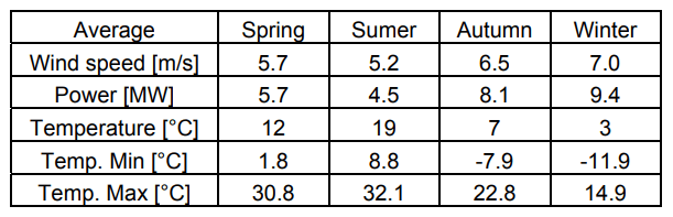
As can be seen from the formulas (1) and (2), besides the wind speed there are also other factors that determine the volume of energy production including temperature, humidity or pressure. The table 1 provides additional information about changes to this parameter depending on the season.
Table 1. Summary of characteristic parameters of wind power generation in a seasonal view
.
The average wind speed varies slightly depending on the season, the difference is only 1.8 m/s. Bigger differences are observed for parameters like average, minimum and maximum temperature. An undesirable situation is lowering the temperature below 0°C, which may cause icing of windmill blades. This phenomenon changes the aerodynamics of the blades of windmills and it can result in a significant reduction in the generated electric energy, and in extreme cases, it might cause a damage to the fan. Below zero temperatures were registered in autumn and winter. During this period, a strong increase in the average 15-minute power of a wind farm was observed. An increase of 3.6 MW (autumn) and 4.9 MW (winter) compared to the summer, which is over 52% and 70% of the power-to-average power farm for this season.
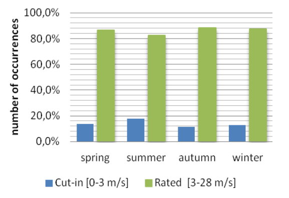
Unwanted operating states of wind farm
Over the years 2012-2014 the speed of the wind has varied widely. In order to ensure the safety and maximize the efficiency of wind, farm turbines are subject to restrictions due to the speed of the wind. For the considered wind turbines three ranges of wind speed are defined: Cut-in Wind Speed (0-3 m/s), Rated Wind Speed (3-28 m/s) and Cut-out Wind Speed (more than 28 m/s). An analysis of the frequency of farms in these speed ranges for the data from the years 2012-2014 showed no incidents causing an emergency shutdown of the turbine due to too strong wind (Cut-out Wind Speed more than 28 m/s). During vast majority of 15-minute measurements (over 80% of all measurements), wind speed was in the range of normal operation of the wind farm. The differences in the size of the datasets, depending on season, were in the range of ±6,1%.
Fig.10. Percentage of the number of occurrences for operating mode – four seasons
Because of the climatic conditions in Central Europe, temperatures falling below 0 Celsius degrees, it is necessary to take into account the additional phenomenon of ice on the blades of a windmill. This phenomenon changes the aerodynamics of the blades of windmills and it can result in a significant reduction in the generated electric energy, and in extreme cases, it might cause a damage to the fan.
Building neural models when considering the seasonality
A. Selecting the forecasting models
This chapter presents the results of prediction of the power output of an onshore wind farm operating with 15 turbines for three different forecasting models. The learning process of the neural network was performed using back propagation (BP-neural network) and the Levenberg Marquard algorithm. The verification of the models was performed using the real weather data. The training sets were selected in such a way to get two full years, including all four seasons.
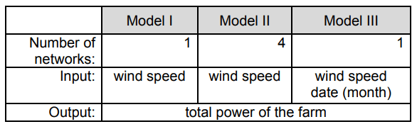
The verifying data sets contains measurements from one full year. Various types and structures of artificial neural networks dedicated to the prediction of the energy in wind farms have been proposed in [4]. ANN have an opportunity to expand, because they can work independently or together with another wind power forecasting method. They both are forms of hybrid structures [5]. Model I is a reference point built on the full annual figures. Model II contains four submodels dedicated to each season independently. Model III takes into account seasonal phenomenon in the form of information about the month for which the forecast was made.
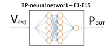
Model I –Pout = f (Vavg)
The first and the simplest model forecasts produced power depending on the average wind speed for the entire wind farm. The operating rules of the neural network Model I are shown in Fig. 11.
Fig.11. Single BP-neural network on the input average wind speed
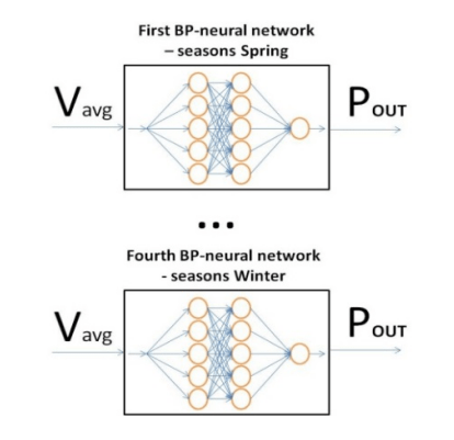
Model II –Pout (seasons) = f (Vavg)
The second model was constructed in a similar way to the first, except that the preparation of four models of learned neural networks using selected data sets for different seasons. As a result, four neural networks for each season separately.
The operating rules of Model 2 are shown in Fig. 12.
Fig.12. Four neural network for each season independently
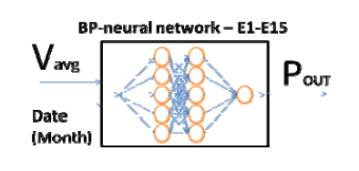
Model III –Pout = f (Vavg ,month )
Model III is similar to the model I and, with the difference that the impact of seasonality as an additional input neural network was taken into account as an additional input for neural network. At the input of the neural network the average wind speed for the entire farm and the number of the month for which projections were made introduced.
The operating rules of Model III are presented in Fig. 13.
Fig.13. – Single BP-neural network, the input average wind speed and the date (month)
where: Pout– output power of the wind park MW, Date (month) – number of the month for which the forecast was made (ranging from 1-12),
.
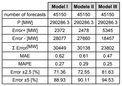
Table 2. Summary of differences between the analyzed models
.
B. Indicators models
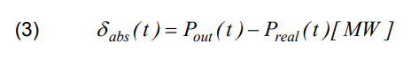
The evaluation of the effectiveness of the models was carried out for a period of one year, by comparing:
• revaluation, underestimation and absolute forecast error
.
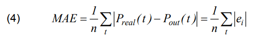
• mean absolute forecast error MAE,
.
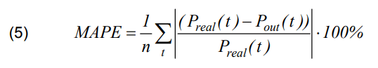
• mean absolute percentage error MAPE
.
Frequency of obtaining the forecast with the accuracy of 0.75 MW and 1.5 MW, which corresponds to ± 2.5% and ± 5% of the installed capacity of wind
Verification and comparison of models
This chapter presents the results of estimation of electricity production for three proposed models. The prediction was made for an onshore wind farm.
The forecasting method, using artificial neural networks to generate satisfactory results enables the predictions. When considering selection of a variety of structures, a strong dependence of the quality of forecasts on the selected training set was observed. Table II presents the results of forecasting accuracy for each model of forecasting for three models.
Table 3. Summary of results forecasts for the proposed models – the annual results
.
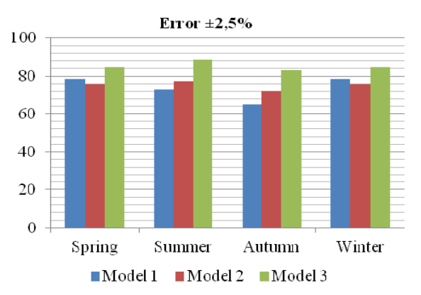
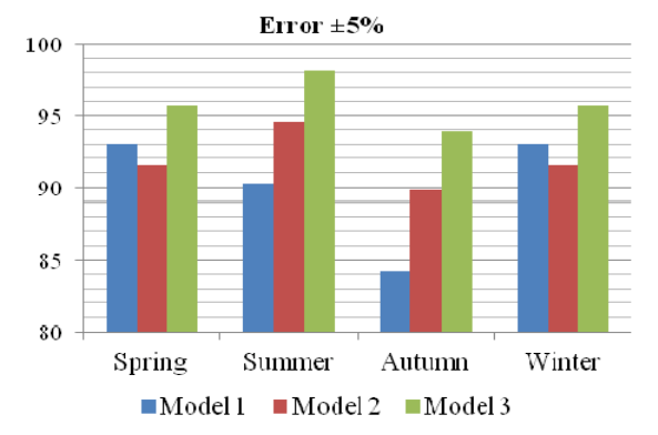
Fig. 14 and Fig. 15 show the results of forecasting accuracy for different seasons:
Fig.14. The accuracy of forecasts – the percentage of errors coming within + -2.5% of installed capacity
Fig.15. The accuracy of forecasts – the percentage of errors coming within + -5% of installed capacity
Conclusion
The long-term electrical and meteorological data from three years of wind farm operation (covering seasonality impact) were used to examine the forecast methods based on three different neural network models.
The analysis of measuring data confirmed the impact of the seasons, and thus the impact of cyclical changes on the energy production volume. The changes of wind speed and temperatures have a significant impact on the operation of the wind farm. The largest volume of energy production was recorded in autumn and winter. The smallest average energy production was registered in summer. Despite an insignificant increase in average wind speed in fall and winter, the average energy production changed noticeably, in the autumn there was an increase of 80%, and in winter, an increase of over 108% compared to summer in which production was the smallest.
Due to the seasonal changes of meteorological phenomena 3 models of neural networks optimized for the impact of seasonality on working wind farm have been proposed and compared. The third model was the best, but it need long-term data. At the of input of the model information about wind speed and the month for which the forecast energy production was carried out, has been given. Such incorporate cyclic phenomena in this case turned out to be most effective. The disadvantage is the need for a large training set to train the neural network. Such a set would allow to prepare a wide range of forecasts of energy from a wind farm. Too little data may result in not full restoration of the power curve of a wind farm. For summer and autumn a bit better was Model II prepared on selected data for individual seasons. For spring and winter the simplest Model I turned out to be slightly better than the Model II.
REFERENCES
[1] Całus D., Oźga K., Popławski T., Michalski A., Szczepański K., Możliwości i horyzonty ekoinnowacyjności – Zielona energia, Wydawnictwo Instytut Naukowo-Wydawniczy “Spatium”, Częstochowa 2018 [2] Popławski, T., Weżgowiec M., Krótkoterminowe prognozy cen na Towarowej Giełdzie Energii z wykorzystaniem modelu trendu pełzającego, Przegląd Elektrotechniczny, 91, (2015), nr 12, 267-270 [3] Ciechulski T., Osowski S., Prognozowanie zapotrzebowania mocy w KSE z horyzontem dobowym przy zastosowaniu zespołu sieci neuronowych, Przegląd Elektrotechniczny, 94, (2018), nr 9, 108-112 [4] Yuan-Kang Wu, Po-En Su, Ting-Yi Wu, Jing-Shan Hong, Yusri M. H., Probabilistic Wind-Power Forecasting Using Weather Ensemble Models, IEEE Transactions on Industry Applications, (2018), 54, 6, 5609-5620 [5] Yang M., Lin Y., Zhu S., Han X., Wang H., Multi-dimensional scenario forecast for generation of multiple wind farms, Journal of Modern Power Systems and Clean Energy, 2015, 3, 3, 361-370 [6] Ciu M., Ke D., Gan D., Sun Y., Statistical scenarios forecasting method for wind power ramp events using modified neural networks, Journal of Modern Power Systems and Clean Energy, 2015, 3, 3, 371-380 [7] Safari N., Chung C. Y., Price G. C. D., Novel Multi-Step ShortTerm Wind Power PredictionFramework Based on Chaotic Time Series Analysisand Singular Spectrum Analysis, IEEE Transactions on Power Systems, (2018), 33, 1, 590-601 [8] M. Qi, G. P. Zhang, Trend Time Series Modeling and Forecasting With Neural Networks”, IEEE Transactions on neural networks, vol. 19, no. 5, May 2008 [9] D. Wu, H. Wang, Application of BP neural network to power predioction of wind power generation unit in microgrid, Engineering Technology and Applications, London 2014. [10] Z. Liu, W.Gao, Y.-H. Wan, E. Muljadi, “Wind Power Plant Prediction by Using Neural Network”, IEEE Energy Conversion Conference and Exposition, August 2012 [11] Wen-Yeau Chang, “Short-Term Wind Power Forecasting Using the Enhanced Particle Swarm Optimization Based Hybrid Method, Energies, (2013), 6, 4879-4896
Authors: mgr inż. Mateusz Dutka, AGH University of Science and Technology, Department of Power Electronics and Energy Control Systems, 30 Mickiewicza Ave., 30-059 Krakow, POLAND, E-mail: mdutka@agh.edu.pl; dr inż. Bogusław Świątek, AGH University of Science and Technology, Department of Power Electronics and Energy Control Systems, 30 Mickiewicza Ave., 30-059 Krakow, POLAND, E-mail: boswiate@agh.edu.pl.
Source & Publisher Item Identifier: PRZEGLĄD ELEKTROTECHNICZNY, ISSN 0033-2097, R. 95 NR 7/2019. doi:10.15199/48.2019.07.25
Published by Electrotek Concepts, Inc., PQSoft Case Study: Transformer Derating, Document ID: PQS0324, Date: October 10, 2003.
Abstract: A principal effect of harmonic distortion is to increase losses and heating in almost every component in the electric power system. While contributing almost no useful work, harmonic components of voltage and current increase the RMS value of voltages and currents. Interaction of harmonic quantities and resistive loss mechanisms in power system components generates excess heat.
Power transformers are also affected by harmonic distortion. Distortion of transformer load current is the most significant impact, leading to higher than normal temperatures at “hot spots” within the windings.
This case presents an evaluation of transformer derating due to harmonic current.
PROBLEM STATEMENT
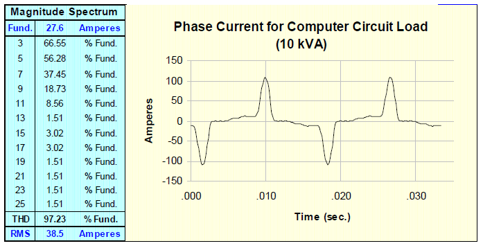
120 Volt, 75 kVA Transformer supplying computer workstations was running very hot at an office building. A check of the load current that the transformer was supplying showed that the amperage level was below the transformer rating. A spectrum analyzer was used to record the following waveform (Figure 1).
Figure 1 – Load Current Waveform and Spectrum
TRANSFORMER DERATING
A principal effect of harmonic distortion is to increase losses and heating in almost every component in the electric power system. While contributing almost no useful work, harmonic components of voltage and current increase the RMS value of voltages and currents. Interaction of harmonic quantities and resistive loss mechanisms in power system components generates excess heat. Some losses are actually sensitive to frequency, so that the power loss per ampere of harmonic current is actually greater than that for fundamental frequency currents.
Power transformers are also affected by harmonic distortion. Distortion of transformer load current is the most significant impact, leading to higher than normal temperatures at “hot spots” within the windings. If harmonic distortion of the load current is high, transformers must be derated to account for the increased heating effect of the distorted current. Guidelines for transformer derating are detailed in ANSI/IEEE Standard C57.110.
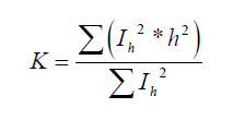
K-Factor Definition
K-Factor is defined in UL Standards 1561 (low voltage) and 1562 (medium voltage) as:
.
where: h……………………………………………………………..harmonic number Ih……………………………………………………harmonic current (amps)
Transformer Derating Using C57.110
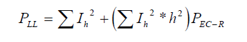
ANSI/IEEE Standard C57.110 applies to general-purpose transformers that are subjected to a load current with a total harmonic distortion greater than 5%. The object of the standard is to determine the value of nonlinear current which results in transformer heating equal to that produced when the transformers is supplying rated linear load. Transformer derating can be determined using:
.
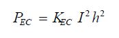
where: PEC-R ……….Eddy current loss at hot spot under rated conditions
Transformer derating depends upon the per-unit rated eddy current loss factor at the hot spot (PEC-R). This factor can be determined by:
1. Obtaining the factor from the transformer designer 2. Using transformer test data and the procedure in C57.110 3. Typical values based on transformer type and size
Table 1 – Typical Values of PEC-R
Reference: “Adjustable-Speed Drive and Power Rectifier Harmonics. Their effects on Power System Components”, D.E. Rice, IEEE No. PCIC-84-52 / *Applies to any transformer with LV sheet type winding
Table 2 summarizes the calculations required to determine the transformer derating and K-Factor for the load waveform illustrated in Figure 1.
Table 2 – Transformer Derating Calculations
.
The K-Factor for the illustrated waveform is determined to be
.
and the transformer derating value is
.
Note: PEC-R assumed to be 8% for this case
Effect of PEC-R
The impact of PEC-R on transformer capability is summarized in Figure 2. As can be seen from the figure, as the eddy current loss factor increases the load current that can be supplied is reduced.
Figure 2 – Transformer Capability vs. PEC-R
SUMMARY
The K-Factor for the load current illustrated in Figure 1 was determined to be 7.56 and the transformer derating value was found to be 82% of it’s rated load current.
This means that the customer has several options when purchasing a transformer to supply this load:
− A 75kVA transformer with a K-13 rating (next standard size chosen) − A K-1 transformers with a 91.5kVA (75/0.82) rating
REFERENCES
Reference: “Adjustable-Speed Drive and Power Rectifier Harmonics. Their effects on Power System Components”, D. E. Rice, IEEE No. PCIC-84-52. IEEE Recommended Practice for Electric Power Distribution for Industrial Plants (IEEE Red Book, Std 141-1986), October 1986, IEEE, ISBN: 0471856878 IEEE Recommended Practice for Industrial and Commercial Power Systems Analysis (IEEE Brown Book, Std 399-1990), December 1990, IEEE, ISBN: 1559370440
Published by Raghavan Venkatesh, EE Power – Technical Articles: Clean Power for Office Towers, April 12, 2018.
This article features EPCOS AG product PQSine S series designed for 3-phase grids with or without neutral conductors and enables harmonics to be filtered.
The complex power networks of skyscrapers and other modern buildings must serve a wide range of nonlinear loads. Cutting-edge active power conditioning solutions based on the EPCOS PQSine S series of active harmonic filters help skyscrapers and large commercial buildings eliminate potential power quality issues.
The many power electronics systems in use in large commercial buildings such as skyscrapers include nonlinear loads such as variable speed drives, UPS systems, computers and servers, lighting, TV sets, and more. A major challenge facing building operators is the harmonics pollution in their power networks, leading to a marked deterioration in the quality of the supply voltage.
TDK field applications engineers are joining forces with specialized power quality distribution partners to create cutting-edge power conditioning solutions for such buildings based on the PQSine S series of active harmonic filters.
The Danger of Harmonic Pollution
The nonlinear current draw results in harmonics that cause distortion in the sinusoidal voltage, which in turn can cause interference for other loads. Harmonics are integer multiples of the basic frequency, i.e. of the line frequency of 50 Hz or 60 Hz. The harmonics have varying amplitudes and can extend into the upper kHz range. Harmonic pollution has a series of negative effects on power quality, including:
• malfunctions of other loads due to poor grid power quality; • additional current load on the neutral conductor, as the harmonic currents of the 3rd, 9th, 15th, and 21st orders, and more. are accumulative and lead to inadmissibly high currents; • phase asymmetry (specifically when operating single-phase switch-mode power supplies) which additionally promotes the generation of harmonics.
In addition, harmonics can severely impair the function of sensitive devices or even destroy them. IT networks with their servers and PCs are a typical example, where the malfunction of network devices can lead to corrupted data and enormous consequential damage.
Towering Power Quality Challenge
Due to the sheer size of skyscrapers and the complexity of its various electrical loads and systems, power quality, therefore, plays a central role in ensuring the lowest possible energy consumption and costs, as well as avoiding overheating, production/process downtimes, and malfunction of equipment.
The major electrical loads and their characteristics are:
Elevators
The required reactive power compensation for up to more than 100 elevators is very dynamic, and changes very fast between capacitive and inductive during operation and when they feed recuperative power back into the network. The THD-I is also very high and changes rapidly. The main contributors to THD are in the 5th, 7th, 11th, and 13th orders.
Indoor and outdoor lighting
All lights are LED and CFL (compact fluorescent lamp), which are used to save energy, generate significant harmonic distortion in the range from 150 Hz up to 2500 Hz. Large-screen LED digital billboards (with up to more than 2000m² dot-matrix lighting); the main harmonic current is of the 3rd order, but harmonic distortion is also present up to the 50th order.
Air-conditioning
The inverters employed are a source of harmonic distortion and require reactive power compensation. They produce dominant harmonics typically in the 5th, 7th, 11th, and 13th order, but also in the 17th and 19th order and above.
Fans, water pumps, cooling machines, and fire protection
The many smaller 6-pulse power converters in the system contribute current harmonics in the 5th and 7th order and above.
IT networks, UPS, security systems, and access control systems
The many SMPS in the servers, clients and other network devices generate harmonics from the 3rd to 23rd order and above. Moreover, they require a reliable and secure power supply without interruptions.
Complete Power Conditioning Solution
The extremely complex load profile of skyscrapers requires both dynamic reactive power compensation and the mitigation of harmonics over a broad frequency spectrum. An ideal solution for such large commercial towers is a complete power conditioning solution based on the PQSine S series of active harmonic filters. The first step is a detailed analysis of the building’s power network. In this case, TDK field application engineers work together with specialized power quality distribution partners. For new skyscrapers, this will take place during the building’s construction phase. Such analyses generally reveal significantly elevated THD levels and transient harmonics in all feeders of a building’s network (Figure 1).
Figure 1: Typical performance analysis of a power supply system, showing the presence of significant harmonic distortion in all harmonics, especially in the 3rd, 5th, 7th, 11th, and 13th orders.
In a typical office tower distortion is especially high in the 3rd, 5th, 7th, 11th, and 13th harmonics. Based on the analysis and the requirements for power quality, energy savings, reliability, the advanced PQSine S series of active harmonic filters and power optimizers represents an ideal solution (Figure 2). The PQSine S series extends the comprehensive portfolio of EPCOS components and systems for power quality solutions covering solutions such as active and passive harmonic filters, detuned capacitor banks, and low and me
Figure 2: EPCOS PQSine S series of active harmonic filters can be installed in-floor cabinets (left) or wall-mounted cabinets (right)
PQSine S Series for High Performance and Reliability
The PQSine S series is designed for 3-phase grids with or without neutral conductors and enables harmonics of up to the 50th order (2500Hz/3000Hz) to be detected and filtered. In addition to outstanding filtering capabilities, PQSine active harmonic filters also ensure balancing of the loads to all three phases. Moreover, neutral conductor currents are also compensated when using 4-wire devices. These features avoid line resonance and ensure high performance and reliability.
Figure 3: Functional principle of EPCOS PQSine. PQSine ensures a sinusoidal current draw. Harmonics and phase shifts are effectively reduced.
The optimized active harmonic filtering solution with PQSine has the following key features:
• Harmonic and reactive power compensation dual function. The PQSine S series of active filters effectively compensate system harmonics, while at the same time providing fast reactive power compensation for both capacitive and inductive loads, which can keep the system power factor at very nearly 1.0.
• Intelligent switching design special bus system, to ensure that any two of the three ACB cabinets (two incoming and one bus coupler) are always switched in for performance and redundancy purposes.
• Ultrafast reaction speed The PQSine S series of active filters feature a reaction time of under 50 μs and can thus respond quickly to the high and rapidly changing loads;
• Modularity and scalability In order to allow for future system expansion to meet changing power conditioning requirements, each installed PQSine cabinet has two or three empty slots.
Optimum reliability is ensured by means of a series of self-monitoring systems. The most important of these are overload protection, shutdown on overtemperature, protection against overvoltage or undervoltage and fan monitoring. The PQSine S series includes a 7-inch TFT color touch-screen for user-friendly input and reading of the data. PQSine offers a number of Modbus (RTU) and TCP/IP (Ethernet) interfaces for control, programming, and diagnostics purposes.
The PQSine S series of active harmonic filters are based on the latest state of the art in power electronics technology. They are installed in parallel to the polluting loads. The active filter analyzes the line current and its associated harmonics and generates a compensation current which neutralizes the harmonic currents and creates an almost sinusoidal waveform (Figure 3). With its fast reaction time, PQSine offers excellent performance for fast-changing loads, such as those generated by elevators. Using the data determined in real-time, PQSine feeds a compensation current into the grid, which cancels the nonlinearity of the load current.
Optimized design for demanding harmonics order to optimally compensate harmonic currents from the electrical loads in a recent installation, a total of 76 PQSine S series units were installed for the various feeders on eleven levels of the skyscraper. Figure 4 shows a typical single line diagram of an electrical distribution board.
Figure 4: Typical single line diagram of an electrical distribution board.
Reliable Harmonic Current Compensation for a Wide Range of Applications
After the installation of the complete power conditioning solution, the TDK field application engineers and their partners typically perform a comprehensive power quality analysis with a specific focus on harmonics as proof of the installation’s effectiveness. According to the power quality data gathered on-site at a recent installation, the PQSine S series limits the system THD-I to below 3 percent. The system current was about 160 ARMS during the specific measurement. Overall, the PQSine solution successfully delivered the highest level of power quality. The current phases were sinusoidal with a very low level of THD-I (Figure 5), and the power factor was nearly 1.0.
Figure 5: With the PQSine active harmonic filter and power optimizer, the current phases were sinusoidal with a very low level of THD-I and the power factor was nearly 1.0.
PQSine has proven very effective in mitigating harmonics and also providing dynamic reactive power compensation to ensure the optimal power quality for all loads and users of large commercial buildings. PQSine active harmonic filters and power optimizers are especially suitable for fast current harmonics, reactive power compensation or neutral current compensation in a wide range of power networks in
• Data centers and IT-enabled service facilities, • Renewable energy power generation, • Process industries, • Sensitive manufacturing facilities, and • Office buildings, shopping centers, hospitals.
Author: Venkatesh Raghavan holds a Ph.D. and a Master’s Degree in High Voltage Engineering at the Indian Institute of Science and at the Anna University respectively. He also holds a Bachelor’s Degree in Electrical and Electronics Engineering. He is currently the President of EPCOS since February 2008.
Published by Electrotek Concepts, Inc., PQSoft Case Study: PQ Investigation for SW County School District No. 1, Document ID: PQS0323, Date: October 10, 2003.
Abstract: The County School District has a concern for increasing computer loads at the local High School. There are approximately 300 computers currently in use at the school and plans are to increase the number of computers significantly over the next 3-4 years. The existing computer loads are on the same circuits with lighting loads, other office loads, and building HVAC loads.
Electrotek Concepts conducted a brief survey of the facility on August 8, 1995. This case study describes the findings from the site survey and outlines recommended procedures for dealing with the new computer loads.
INTRODUCTION
The County School District has a concern for increasing computer loads at the local High School. There are approximately 300 computers currently in use at the school and plans are to increase the number of computers significantly over the next 3-4 years. The existing computer loads are on the same circuits with lighting loads, other office loads, and building HVAC loads.
The personal computer loads are characterized by a current waveform that has significant harmonic components. These harmonic components are dominated by the third harmonic which appears in the zero sequence circuit (for balanced circuits), which means that the third harmonic components add in the neutral. The result can be neutral circuits which are significantly overloaded if they are not designed for this type of load. The harmonic components can also require derating of the transformers that supply the computer load.
Wiring and grounding considerations are also important with the computer loads. High neutral currents from the PC loads can also flow in the ground circuits if there are incorrect neutral-ground bonds in any sub-panels or loads. The ground currents can cause interference, improper operation of protective devices (breakers), and safety concerns.
System Configuration
The high school is supplied from a 1000 kVA transformer that steps down to 480 Volts. There are a number of transformers that then step down from 480 volts to 120/208 for the various loads in the facility. Figure 1 gives an overview of the system configuration. The 500 kVA transformer supplies most of the load in the main building. The 300 kVA transformer was added for the auditorium load.
Figure 1 – One-Line Diagram on the Main Supply to the High School
Concerns Evaluated
Important concerns evaluated in the site survey and summarized in this report include:
• Harmonic generation from nonlinear loads. • Overloading of neutral conductors due to harmonic current levels. • High voltage distortion on the auditorium circuits. • Transformer derating considerations for harmonic currents • Wiring and grounding concerns at building panels and loads. • Requirements for main transformer rating in the future.
HARMONIC GENERATION BY NON-LINEAR LOADS
Harmonic currents result from the operation of nonlinear loads in the system. These include adjustable speed drives for fan motors and chiller compressors in HVAC systems, fluorescent lighting (with or without electronic ballasts), electronic dimmers for lighting, and electronic power supplies for computers and other electronic equipment.
These nonlinear loads look like sources of harmonic currents to the rest of the system. Voltage distortion results as the harmonic currents flow through the impedance of the conductors, transformers, and system. Longer conductor runs will result in higher voltage distortion levels due to the higher impedance of the circuit.
Measurements were performed previously at the high school to characterize some of these loads. Important results are included here for illustration purposes. These include measurements of the harmonic distortion in the stage lighting circuits which use electronic dimmers and measurements of a typical circuit that is dominated by computer loads.
Harmonics from Computer Loads
Panel PE is a typical panel that supplies computer loads at the high school. Measurements were performed for the total load at Panel PE. Figure 2 below gives an example of the waveform measured.
Figure 2 – Current Waveform for a Circuit serving Computer Load Based on Measurements at Panel PE (adjusted to an equivalent three phase load level of 10 kVA)
A summary of the three phase measurements at Panel PE are provided below in Table 1.
Table 1 – Panel PE Measurement Results
.
Note that the neutral current is higher than the phase current at this panel. The neutral current would even be higher if the three phase currents were balanced. In the balanced case for load current waveforms like the one in Figure 2, the neutral current can be as high as 173% of the rms phase current. It will be dominated by the third harmonic component since this is the component that adds in the neutral.
Harmonics in the Auditorium Dimmer Circuit
The stage lights for the auditorium in the high school use electronic dimmers which result in significant harmonic generation. The harmonic content of these load currents depends on the actual load level. When the dimmers are near full load, the percentage harmonic component is not as great but the load current magnitude is higher. At light loads, the percentage distortion is high but the load current is lower.
Measurements were performed at three different load levels to illustrate this characteristic. The results are summarized in Table 2 and example waveforms are provided in Figure 3.
Table 2 – Current and Voltage Measurements for the Stage Lighting Circuit
.
Figure 3 – Lighting Circuit Load Currents at Different Operating Levels.
Note that the highest voltage distortion levels for this circuit occur when the lighting is near 50% load. At this operating point, the actual amperes of harmonic current components are the highest. The voltage distortion is high because the circuit supplying the lighting has a high impedance due to the long 120 volt circuit supplying this load. The impedance would be much lower and the distortion would be reduced if the auditorium load was supplied with a 480 volt circuit and the step down transformer was installed closer to the auditorium.
EVALUATING NEUTRAL CONDUCTOR LOADING DUE TO HARMONICS
Single phase nonlinear loads can have significant harmonic components at triplen frequencies (3, 9, 15, etc.). When these loads are combined in a three phase circuit, the triplen harmonics show up as zero sequence components. That means they add in the neutral. If there are 10 amps of third harmonic on each phase in the three phase circuit, the neutral current will include 30 amps of third harmonic.
For this reason, neutral currents in 120/208 circuits in many commercial buildings are actually higher than the phase currents. The neutral currents are dominated by third harmonic components from single phase electronic loads, like Pcs. Figure 4below illustrates a typical case in a circuit dominated by PC loads.
Figure 4 – Phase currents and neutral current for a circuit dominated by single phase electronic loads.
The rms neutral currents in this type of circuit can be as high as 173% of the rms phase current. The actual neutral current magnitude will depend on how much of the load on the circuit has a waveform like the ones in Figure 4.
An approximate formula for calculating the neutral current magnitude as a percentage of the rms phase current is given below. The formula is based on the assumption that the circuit loading is balanced, that the nonlinear load watts are a pnl fraction of the total load, and that the load current has a third harmonic component equal to 70% of the fundamental.
.
This relationship is illustrated in graphical form in Figure 5.
Figure 5 – RMS neutral current as a function of the portion of electronic load in the circuit, pnl.
It is important to note that the neutral current problem is usually restricted to 120/208 volt circuits supplying a significant percentage of single phase electronic load. Neutral currents are very seldom a problem at service entrance locations, due to delta-wye transformers and harmonic cancellation between different types of loads.
The figure shows that the neutral current will be equal to the phase current when approximately 50% of the load on the circuit is electronic loads. For circuits with higher percentages of electronic load, the neutral current will exceed the phase currents. If these circuits are loaded based on the capacity of the phase conductors, the neutral conductor could be overloaded.
Possible solutions to the neutral conductor overloading problem include the following:
− increase the neutral conductor size or use two neutral conductors. − use a separate neutral for each phase conductor. − apply a third harmonic filter at individual loads. − use an isolation transformer, zig-zag transformer, passive filter, or active filter (three phase devices) on the load side of the neutral conductor to be protected.
Implications for SW County High School
With the number of PCs planned and existing at the high school, a number of circuits will be dominated by electronic loads. There is a concern for neutral conductor loading on these circuits. Panel PE and Panel I are examples of panels that supply load that is dominated by PCs.
Most existing circuits do not seem to be loaded close to their rating. In addition, circuits examined have neutral conductors that are the same size as phase conductors (they could be undersized according to the code). As a result, neutral conductors are not being overloaded at the present time. Circuit loading should be reviewed periodically on circuits that are dominated by computer load to assure that neutral conductors are not being overloaded.
New circuits that are installed to supply future PC loads should have neutral conductors that are sized for this type of load. Neutral conductors in new circuits supplying pc loads should have a rating of about twice the phase conductor rating.
TRANSFORMER DERATING REQUIREMENTS
Transformer heating is one of the primary concerns associated with harmonic current distortion levels in a facility. ANSI/IEEE Standard C57 series states that a transformer can only be expected to carry its rated current if the current distortion is less than 5%. If the current distortion exceeds this value, then some amount of derating is required. ANSI/IEEE Standard C57.110 provides calculation procedures that can be used to evaluate the required derating as a function of the expected current harmonic spectrum and the transformer design. The primary cause of the concern is that the transformers can be overheated by distorted load currents that cause higher eddy current losses inside the transformer than were anticipated by the designer.
At the inner winding “hot-spot”, the load loss (PLL) can be considered to have two components: I2R loss and eddy current loss (PEC). The relationship is given by:
.
The I2R loss is directly proportional to the square of the rms value of the current. However, the eddy current loss is proportional to the square of the current and frequency. It is defined by:
.
where:
KEC = a design-dependent proportionality constant
With all values expressed in per unit of rated load quantities, the per-unit full load loss under harmonic current conditions is given by:
.
where:
PEC-R = eddy current loss factor under rated conditions
The required transformer derating is calculated based on the additional heating that can be expected for a specific harmonic current spectrum and the eddy current loss factor for the transformer. The derating is expressed as the per unit value of a particular distorted current that will cause the same heating as the rated sinusoidal current.
The first task is to measure, calculate, or estimate the harmonic content of the transformer load current. Then, the expected harmonic current spectrum can be used to calculate the k-factor of the load current. The k-factor of the load current can be used to purchase a transformer that is designed to handle the level of harmonic distortion specified. The k-factor is only dependent on the current waveform. There is no need to get any information about the transformer design in order to use the k-factor. K-factor is calculated using the following formula.
.
The increased transformer losses at harmonic frequencies are caused by increased eddy current losses. If the transformer has very low eddy current losses, there will not be a significant impact due to harmonic components. If the transformer has high eddy current losses, significant derating will be necessary for harmonic components. The transformer eddy current losses are characterized by the eddy current loss factor, PEC-R. This number can be from the transformer designer, from the transformer test data and the procedure in C57.110, or estimated based on typical values. A typical value for dry type transformers used to step down from 480 volts to 120/208 volts within facilities is about 8%.
The transformer derating is expressed as the per unit rms current (with distortion) that will cause the same heating as the rated sinusoidal current. It can be calculated from the following equation using the transformer eddy current loss factor and the k-factor of the load current.
.
where:
.
PEC-R = eddy current loss factor h = harmonic number Ih = harmonic current
Probably the worst case condition for one of the step down transformers within the facility is virtually 100% electronic load. Figure 6 illustrates the waveform and the required transformer derating for this condition. Note that the k-factor for this waveform is 7.6. A transformer with a k-factor greater than 7.6 could be loaded to its nameplate rating for this load current waveform.
Figure 6 – Required transformer derating as a function of the eddy current loss factor.
Implications for SW County High School
Both of the step-down transformers (500 kVA and 300 kVA) at the high school main switchgear could have relatively high percentages of nonlinear load. However, the nonlinear load is not approaching 100% of the load on the transformer. Also, these transformers do not appear to be operating near their rating at the present time. A conservative limit for these transformers would be 80% of their nameplate ratings. Loading on the high school step down transformers should be monitored periodically and kept below 80% of the transformer rating to prevent overheating due to harmonic components.
New circuits to supply additional PC loads can be supplied from the main 500 kVA transformer as long as the transformer loading is kept below 80% of the nameplate. If new loads will result in this limit being exceeded, additional transformer capacity should be added. A new transformer to supply electronic loads (PCs) should not be loaded above 60% of its nameplate or a transformer with a k-factor rating of 13 should be purchased.
The main supply transformer for the facility (1000 kVA) should not require any significant derating for harmonic components. The step-down transformers prevent the flow of zero sequence harmonics and there is significant cancellation of harmonics for all the loads within the facility. The main supply transformer should not require significant derating for harmonic levels.
WIRING AND GROUNDING CONSIDERATIONS
Many power quality problems that occur within end user facilities are related to wiring and grounding practices. Sometimes the solution to a power quality problem is simply to tighten a loose connection or replace a corroded conductor. Therefore, an evaluation of wiring and grounding practices is a necessary first step when evaluating power quality problems in general.
Check RMS Voltage Levels
Service entrance should be within +/- 5% of nominal volts. Utilization should be within +6, -13% of nominal volts. The long circuit runs required when the step down transformers are located at the main switchgear can result in reduced voltage magnitudes at the actual loads. Measurements at various panels in the high school show that the voltage can be as low as 110 volts. This should not result in any problems.
Check for extra neutral-ground bonds
There should be only one neutral-to-ground bond per separately derived system (at the transformer or at the main panel). This is a common problem which causes load currents to flow in the building ground system, creating the potential for serious interference problems. This can be checked by measuring the current in the green wire grounds at the service entrance or at the source of the separately derived system. These currents should be very close to zero. If any current is flowing in the ground, the source of the current should be found and corrected.
Visual inspection of a couple sub panels at the high school indicated that the neutral bus in some sub panels may be grounded. Figure 7 below illustrates the possible problem that can be caused by this extra neutral-to-ground connection – some of the neutral return current is introduced into the ground system where it can cause interference.
Figure 7 – Introduction of neutral return current into the ground system (caused by an extra neutral-to-ground connection
Check for overloaded neutral conductors
This has already been discussed related to supplying electronic loads with high third harmonic current components. The neutral currents should be measured with a true RMS meter and checked against the ampacity of the neutral conductors.
Checking grounding electrode system
The grounding electrode system consists of all the grounded elements of the building that are bonded together to form a grounding system. This can include ground rods, metal water pipe, building steel, concrete-encased electrodes, a ground ring, etc. All of these things should be bonded together to form the best equipotential reference for equipment in the building as possible.
It is not advisable to have separate, isolated ground rods for individual equipment in the facility. If a separate ground rod is driven for equipment, it should be bonded with the overall building grounding electrode system.
Guidelines for the grounding electrode conductor are provided in Table 3.
Table 3 – Guidelines for the grounding electrode conductor size.
.
Overall circuit layout considerations
Are sensitive equipment loads on separate circuits from disturbing loads? Loads that are switched or that have power electronic components create transient disturbances which can impact the operation of some sensitive equipment. Loads like switched motors, copiers, laser printers, elevators, etc. should be on separate circuits from sensitive equipment. The separate circuits provide isolation for high frequency transients and a clean ground reference for the sensitive loads.
For new computer loads at the high school, dedicated circuits could be designed with additional neutral capacity to handle the harmonic components.
Separately derived systems
Separately derived systems permit the bonding of the ground and neutral. In circuits with significant neutral currents (e.g. single phase electronic loads), a significant neutral-to-ground voltage will build up if there is a significant length between the loads and the supplying transformer. Using an isolation transformer close to the loads minimizes the neutral-to-ground voltage and also provides isolation for transient overvoltages.
Check for ground loops
Ground loops are probably the most common cause of interference in network systems and also the most common problems with multi-port devices in general. Multi-port devices have more than one type of interface. For instance, a television has a power input and a cable input; a computer has a power input and a phone input for the modem and a network input for a LAN. All of these ports require a ground reference. This multiple ground reference scenario creates the potential for serious ground loop problems.
Ground loops problems are best avoided by making sure all equipment that is tied together through other ports (e.g. on a LAN) has the same ground reference. This means that all the equipment is part of the same separately derived system. Figure 8 illustrates this as the grounding bubble principle. If an external ground reference goes outside the bubble, there is the potential for ground loop interference.
Figure 8 – Example system illustrating the bubble principle of grounding (All equipment with other ground ports to the same power system ground reference. Figure is courtesy of Scott Peele at Carolina Power and Light.)
Implications for Sweetwater County High School
The most important wiring and grounding concern at the high school is extra neutral-to-ground connections at sub panels. Most of the circuits from the main switchgear to the sub panels use conduit grounding. The sub panels should not have the neutral bus connected to the ground bus and case in the panel. This extra connection could result in loss of overcurrent protection for these circuits and interference concerns when PCs are connected up in networks.
New circuits for computer loads should include a separate green wire safety ground conductor. This will facilitate checking for unwanted ground currents in these circuits.
New circuits for computer loads should use a step down transformer as close to the loads as possible. This will prevent excessive neutral-to-ground voltages and long lengths of circuit with high neutral currents that could cause interference.
EVALUATING THE MAIN TRANSFORMER REQUIREMENTS
The addition of new computer load could result in the need for additional transformer capacity in the main supply from the utility. This depends on the existing load levels for the 1000 kVA supply transformer.
The utility performed some measurements at the 480 volt service entrance last year but these were primarily designed to evaluate harmonic distortion levels. Measured levels were compared to the IEEE 519-1992 guidelines and harmonic current levels were not found to be a problem. Some of the plots included with the report appear to be the result of either transient inrush conditions or caused by saturation of Cts (high even harmonic current components should not exist in the steady state). These should not be representative of the normal harmonic current components. As stated in the report, normal harmonic current levels are well within guidelines and should not result in the need for derating of the main transformer.
It would be useful if additional measurements could be performed to characterize the existing transformer loading as a function of time. This would provide a benchmark for evaluation of future transformer capacity requirements.
If the supply transformer is replaced with a larger unit, it should be sized based on the expected future loading at the high school, including the ultimate level of computer penetration.
SUMMARY
General Recommendations
− Harmonic voltage distortion can be high on the auditorium lighting circuits due to the dimmer loads and the high impedance created by the overall circuit length. The voltage distortion could be reduced if the step-down transformer for these circuits was located closer to the loads. Even though the voltage distortion is high, it should not be a problem for the lighting circuits.
− If the voltage distortion on these lighting circuits needs to be reduced, the most economical solution would be a zig-zag transformer applied close to the lighting loads. This would reduce the zero sequence components and the corresponding voltage distortion. The transformer is rated in zero sequence amps. A transformer rated for approximately 250 amps would be needed based on the measurements.
− Existing computer loads are resulting in neutral current magnitudes that exceed the phase currents in some circuits. However, the circuits are not heavily loaded. These circuits should be monitored periodically to make sure that neutral conductor capacities are not exceeded.
− New computer loads can be supplied with dedicated circuits that have a neutral conductor rated for twice the current of the phase conductors.
− Loading of the facility step-down transformers should be monitored periodically. As a conservative limit, they should not be loaded above 80% of their nameplate capacity. − A new facility step-down transformer dedicated to computer load should have a k-factor of 13 or should only be loaded up to 60% of its nameplate capacity.
− Existing sub panels should be checked for neutral-to-ground connections. The neutral bus in the sub panels should be isolated from the ground bus and the case.
Published by Vishnu SURESH, Dominika KACZOROWSKA, Przemyslaw JANIK, Jacek REZMER, Wroclaw University of Science and Technology
Abstract. This paper deals with load flow analysis of local microgrid containing a stochastic renewable energy source and storage. The study is carried out using the Matpower toolbox with all relevant constraints considered regarding storage, power lines and other components. Certain operational scenarios of the microgrid are also discussed.
Streszczenie. Niniejszy artykuł dotyczy analizy rozpływu mocy w lokalnej mikrosieci zawierającej stochastyczne odnawialne źródło energii i magazynowan energii. Analizę przeprowadzono przy użyciu zestawu narzędzi Matpower ze wszystkimi istotnymi ograniczeniami w odniesieniu do magazynu energii, linii energetycznych i innych komponentów. Omówiono również niektóre scenariusze operacyjne mikrosieci – Analiza rozpływu mocy w lokalnej mikrosieci z magazynem energii
Keywords: Microgrid, Matpower, storage, Renewable energies, Power flow. Słowa kluczowe: Mikrosieci,, Matpower, magazyn energii, Odnawialne źródła energii, Rozpływ mocy.
Introduction
The increasing penetration of renewable energy sources and restrictions on expansion of centralised conventional sources of power has led to research into microgrids.
Microgrids represent a low voltage system hosting a network of distributed energy sources, storage and loads that is tailored to a local environment [2,4]. The energy is generated close to the areas of consumption thereby reducing transmission and distribution losses incurred on account of longer transmission lines along with multiple environmental benefits.
From the point of view of the system operator the microgrid is seen as a single system [4]. The energy sources in the network are stochastic and the problem of energy balance, load flow and power quality become complex. Hence, this paper presents modelling of microgrids, associated load flow problem and its solution employing a MATLAB toolbox named MATPOWER developed by Cornell University [1].
It describes the decision-making process involved with storage connected to the microgrid. The effect of reactive power compensation on overall power demand on the grid and a few operational scenarios.
Current research in this area includes modelling of local microgrids in simulation packages, such as MATLAB [4] and industrial software such as ETAP[6], Matpower also contains numerous test cases of power system models used for load flow and optimal load flow studies that can be found in [1]; typically most cases are related to conventional power systems not containing renewable or sources of a stochastic nature This paper explores its adaptability regarding sources of stochastic nature, In [4] the focus was laid on two different microgrid cases differing in the number of storage units used and a dynamic approach to modelling storage has been introduced which is being adopted in this study on microgrids. In [6] the modelling of the grid took into account the load demand and had included a wind turbine generator as one of the sources. In the present study the load flow is carried out with storage but is modelled as a local scenario. Numerous other methods exist to solve typical load flow problems that involve solving a set of nonlinear equations, they are discussed in detail in [7,8].
Microgrid Components and load flow problem formulation
The system used in this study is a 4-bus network representing a typical configuration of a microgrid located far from the utility grid, similar to the situation of rural areas. Every bus is characterised using four variables as given below [2,5]:
(1) •Pi(t) – Active power injected into the bus •Qi(t) – Reactive power injected into the bus •Vi(t) – Voltage magnitude at the bus •δi(t) – Phase angle of the voltage at bus
Here, i = 1,2,…..,n represents the number of buses in the given network.
The utility grid is taken as the reference bus [5], It is common practice since the utility grid in this scenario would be able to provide active and reactive power according to the needs of the microgrid. The voltage magnitude and angle for a reference(slack) bus is always 1∠0o.
Commonly sources modelled as PV buses [5] have active power and voltage magnitude specified but in reality, solar energy sources exhibit voltage changes during production time, hence, it is more appropriate to model solar sources as a PQ buses as it is done in this study.
Storage is modelled as a PV source [2] and since the time dimension is involved with the operation of storage, a dynamic approach to its modelling is used as described in [2].
Load is modelled as a PQ bus [5]. Reactive power compensation is provided along with solar source at the bus in order to study its influence on the power supply. The shunt capacitor bank used is a Legrand – Automatic – H Type 3 Phase 400 V-50 HZ -75 KVAR. The distribution lines used in the study are NKT low-voltage IEC standard – 60502-1:2004 lines, as described in the Table 1.
Table 1: Cable data
.
In this study the data input for solar PV is obtained from in-house solar panels installed at the Wroclaw University of Science and Technology. The load data obtained is real, one week data utilised for study purposes. The utility grid in this study has been taken as a large generator that would be able to supply active and reactive power as per system requirements to carry out power flow analysis.
The power flow problem involves solving for the above mentioned four variables in (1). The equations are given below.
.
where, i = 1,2,…..,n. Yik– represents self-admittance and mutual admittances and together form the bus admittance matrix which is crucial to obtain values of all parameters at all buses.
Equations (2) represent 2n power flow equations for active and reactive power at all buses and since each bus has 4 variables, the resultant is 4n variables that has to be solved. Since every bus has been assigned a particular bus type, 2 variables are fixed at any given point for a particular bus simplifying the problem to 2n variables. The equations (2) are non-linear algebraic equations, hence it is necessary to apply numerical methods to arrive at a solution [5]. Further information on the theoretical formulation of the problem can be obtained from [5].
There are numerous methods numerous methods available to arrive at a solution for the given problem such as Gauss-Siedel, Newton-Raphson, Fast decoupled load flow methods amongst many others.
In the Gauss-Siedel method, the set of non-linear equations are solved by first assuming a solution vector and by using one of the equations at (2) the revised value of a particular variable is obtained by substituting the other variables in that equation, then the solution vector is updated with regard to this new value. This process is then repeated so as to obtain revised values for all variables and that would complete 1 iteration. This process is then repeated in several iterations until the process converges to a solution with an acceptable accuracy. The gauss Siedel method is considered to be very sensitive with regard to initial solution vector that is chosen [5,10]. If the solution vector chosen is closer to the actual solution then the method will converge faster taking lesser number of iterations, if the solution vector assumed is not accurate then in certain cases the method will fail to converge at a solution.
In order to overcome the issue of performing a large number of iterations in the Gauss-Seidel method, the Newton-Raphson is proposed to solve the set of non-linear equations. [5,10] The Newton-Raphson method is faster at calculating the solution since it is a gradient based solver and the calculation of a Jacobian matrix enables the method to converge on to the solution in a much lesser number of iterations. According to [10] the number of iterations taken for a 500-bus network would be 500 iterations for the Gauss-Seidel method whereas the solution would be arrived in 4 iterations with the Newton-Raphson method. But since the time taken for one iteration is about 7 times in the Newton-Raphson method as in the Gauss- Seidel method the overall gain in speed is about 15 times. Other methods such as the fast decoupled load flow methods further quicken the solution finding process but taking advantage of the weak coupling between (Pi, δi ) and (Qi, Vi) and is typically used in systems consisting of conventional sources of power and long transmission lines[5]. But since, the network used in this study has stochastic sources of energy and shorter distribution lines, the Newton-Raphson method is used for solving power flow equations.
The process involved in running load flow analysis in MATPOWER and the decision-making process involved in storage working is described in a flow chart in Fig. 1
The single line diagram of the setup is as shown in Fig 2. The specifications of all components are also shown. Nominal voltage of the system is 400V.
Fig. 1: Work flow of load flow analysis
Fig. 2: Microgrid network modelled in the study.
Table 2: Component constraints
.
In order to match reality as close as possible all components are subject to constraints that are imposed upon by the hardware itself, type of bus and relevant standards.
Case study results and analysis
The main purpose of load flow is to balance active and reactive power demand and generation as given by the equations below.
.
where PG, QG, PD, QD, PL, QL represent active power generated, reactive power generated, active power demand, reactive power demand, active power loss in the system and reactive power loss in the system, respectively. Figure 3 is a representation of the equations at (3) and it is evident that active and reactive powers consumed and generated match each other hence validating the accuracy of MATPOWER and the simulated system design.
Fig. 3: Active and reactive power match
Fig. 4: Sources output of active power
Fig. 5: State of charge and storage generation output
Fig 6: Reactive power demand from the utility grid with and without compensation
Fig 7: Line losses with (dashed line) and without (solid) reactive power compensation
Figure 4 represents the active power output of the solar PV installation, the active power taken in or exported out to the utility grid and the storage capacity. It is inferred from the plots that initially when the solar PV installation is not producing active power all of the load’s demand is met by the grid and also the storage at this time when it is empty. Later on, during mid-day when solar production increases and reaches peak capacity the load is catered to by the solar PV output and excess is used to charge the storage. Since only a part of the energy can be used to charge the storage at any given point of time, the rest of the energy is exported out to the grid. It is seen that when solar output roughly exceeds the load demand and power is being exported to the grid, the storage device starts to charge. Then, when the solar power output reduces and is smaller than the load demand the storage device comes online and produces power for a short while until it is discharged to a threshold level of 10% of storage capacity.
Figure 5 demonstrates how SOC (state of charge) of the storage device changes with its output and storage capacity. From the Fig. 5 it can be noticed that when the storage output generation increases the state of charge value decreases accordingly.
Numerous devices that are connected to the power system tend to draw reactive power from the sources. High demand for reactive power from the loads cause power quality issues such as voltage fluctuations, increased power losses over lines and also increased MVA demand from sources [9].
Nowadays, when the demand for electricity keeps increasing, utilities are faced with the problem of meeting the demand at lower costs. Hence, it has become common practice for the utilities to place compensation devices along the network to manage demand on the network and to improve voltage profiles.
Many techniques are available for the purpose of compensation, some of them being usage of capacitor banks, static var compensators, synchronous condensers, STATCOMs amongst other many others. They are discussed in detail in [9] with standard models.
Figure 6 makes a comparison of the reactive power demand from the grid with capacitor bank connected and disconnected from the bus. It can be seen that the demand for reactive power is higher without compensation than with compensation. This is because a part of the reactive power demand is provided by the capacitor bank.
Figure 7 represents line losses for cases with and without reactive power compensation. It is evident from the figure that the line losses with reactive power compensation (dashed lines) are lower when compared to the line without compensation (solid lines) for lines ‘1-2’ and ‘1-4’ which are the lines used to export and import power from the utility grid, hence it can be concluded that with reactive power compensation overall reactive power demand is reduced.
Table 3: Summary of findings
.
Conclusions
The study represents a typical microgrid with data that is taken from the real world. Load flow study performed for the network reveals the characteristics with regard to the working of storage and the benefits of localised reactive power compensation. The active and reactive power demand and supply within the network is balanced accurately even though the solar PV and storage system produce energy intermittently and not in a regular manner such as thermal power plants. Moreover, it has been shown that power flow studies can be carried out successfully even when the solar PV source is modelled as PQ bus instead of a PV bus and thus taking into account the fluctuating nature of the solar system voltage.
Further study on the model would be to diversify the sources in the system and carry out optimal power flow using an appropriate optimization technique. Also comparison of the usage of different types of battery storage devices and incorporation of their charging characteristics could be implemented in future studies.
REFERENCES
[1] R. D. Zimmerman, C. E. Murillo-Sanchez, and R. J. Thomas,\Matpower: Steady- State Operations, Planning and Analysis Tools for Power Systems Research and Education,” Power Systems, IEEE Transactions on, vol. 26, no. 1, pp. 12{19, Feb. 2011. DOI: 10.1109/TPWRS.2010.2051168 [2] Yoash Levron, Josep M. Guerrero, Member, IEEE, and Yuval Beck: Optimal Power Flow in Microgrids With Energy Storage. IEEE TRANSACTIONS ON POWER SYSTEMS, VOL. 28, NO. 3, AUGUST 2013. [3] Chris Marnay, F Javier Rubio, and Afzal S Siddiqui: Shape of the Microgrid, Ernest Orlando Lawrence Berkeley National Laboratory. [4] S. Abu-Sharkha,1, , R.J. Arnolde,1, J. Kohlerd,1, R. Lia,1, T. Markvarta,*,1, J.N. Rossb,1, K. Steemersc,1, P. Wilsonb,1, R. Yaoc,1. Can microgrids make a major contribution to UK energy supply? [5] DP Kothari, IJ Nagrath: Modern Power System Analysis, Third edition. [6]. Sneha Kulkarni, Sunil Sontakke: Power System Analysis of a Microgrid using ETAP , International Journal of Innovative Science and Modern Engineering (IJISME) ISSN: 2319-6386, Volume-X, Issue-X [7] V. Del Toro, Electric Power Systems. Englewood Cliffs, NJ,USA: Prentice-Hall, 1992, vol. II. [8] N. P. Padhy, “Unit commitment—A bibliographical survey,” IEEE Trans. Power Syst., vol. 19, no. 2, pp. 1196–1205, May 2004. [9] J. Nyangoma, K. Awodele* COMPARISON OF DIFFERENT REACTIVE POWER COMPENSATION METHODS IN A POWER DISTRIBUTION SYSTEM Department of Electrical Engineering, University of Cap [10] Stott, B. (1974). Review of Load-Flow Calculation Methods. Proceedings of the IEEE, 62(7), 916–929. https://doi.org/10.1109/PROC.1974.9544
Authors: Vishnu Suresh, PhD candidate – Wroclaw University of Science and Technology, Faculty of Electrical Engineering, Wybrzeze Wyspianskiego 27,50-370 Wroclaw, E-mail: vishnu.suresh@pwr.edu.pl; Dominika Kaczorowska, PhD candidate – Wroclaw university of science and Technology, Faculty of Electrical Engineering, Wybrzeze Wyspianskiego 27,50-370 Wroclaw, E-mail: dominika.kaczorowska@pwr.edu.pl, dr hab. inż. Przemyslaw Janik – Wroclaw University of Science and Technology, Faculty of Electrical Engineering, Wybrzeze Wyspianskiego 27,50-370 Wroclaw, E-mail: przemyslaw.janik@pwr.edu.pl , dr hab. inż. Jacek Rezmer – Wroclaw University of Science and Technology, Faculty of Electrical Engineering, Wybrzeze Wyspianskiego 27,50-370 Wroclaw. jacek.rezmer@pwr.wroc.pl.
Source & Publisher Item Identifier: PRZEGLĄD ELEKTROTECHNICZNY, ISSN 0033-2097, R. 95 NR 9/2019. doi:10.15199/48.2019.09.19
Published by Electrotek Concepts, Inc., PQSoft Case Study: Electric Utility Harmonic Study Medium Voltage Filter Design, Document ID: PQS0407, Date: September 30, 2004.
Abstract: This particular utility was experiencing voltage distortion levels throughout their distribution network that were exceeding IEEE Std. 519 limits. One customer, a plastic extrusion plant, was experiencing blown fuses in their switched capacitor banks along with capacitor failure. A harmonic evaluation study was performed on the 34.5kV/12kV network supplying this customer. The scope of the study was to investigate the impact of surrounding capacitor banks on voltage distortion levels and to make recommendations with regards to mitigating the harmonic problem. A medium-voltage harmonic filter was designed and simulated for mitigation effectiveness throughout the distribution system.
INTRODUCTION
The particular electric utility was experiencing voltage distortion levels throughout their distribution network exceeding IEEE Std. 519 limits. One customer, a plastic extrusion plant was experiencing blown fuses in their switched capacitor banks along with capacitor failure. This is believed to be the result of the high harmonic distortion measured throughout the network.
A harmonic evaluation study was performed on the 34.5kV/12kV distribution system that serves the facility and surrounding areas. The scope of the study was to investigate the impact of surrounding capacitor banks on voltage distortion levels. Of particular interest was the impact on harmonic distortion levels that resulted due to the interaction (resonance) between the capacitors and system impedance.
The scope of the harmonic evaluation study included:
− System model development − Evaluation of system frequency response characteristics (resonance conditions) for various operating conditions − Recommendations regarding follow-on field measurements for characterizing utility system and customer (nonlinear loads) distortion levels − Model update to include nonlinear load characteristics − Evaluation of harmonic distortion levels for various operating conditions − Evaluation of possible solutions to excessive distortion levels, including the design and application of harmonic filters
A complete three-phase model of the distribution system supplied by the 69kV/34.5kV transformer was created using Electrotek’s SuperHarm® program. The model was verified for accuracy and then used to perform the frequency scan analysis, distortion simulations, and ultimately the filter design.
System Description
The feeders experiencing problems are both fed from a 69/34.5kV wye-delta transformer, with three 34.5kV feeders feeding the local loads. There are no capacitors on the first two feeders, however, capacitor banks are located throughout one of the said feeders. The customer experiencing problems (plastics plant) has a 600 kvar, 12-step capacitor bank at the 480V level.
A one-line diagram of the system is shown in Figure 1.
Figure 1 – System One-Line Diagram
The system model was implemented using the SuperHarm program. A three-phase model was used to accurately model the effect of transformer connections on harmonic cancellation. The model includes line and cable characteristics, transformers, substation and low voltage capacitors, load, and an equivalent representation of the adjacent system. All distribution and transmission lines were modeled using a three-phase positive/zero sequence impedance model. Linear load was included to provide a realistic amount of system damping for the distortion simulations. Without these loads, the simulation results would be too conservative, especially at or near system resonance.
Measured Data
The electric utility had previously performed measurements throughout the problematic system using a hand-held power quality meter. These measurements were taken between 4/1/99 and 8/12/99. The surrounding distribution network experience voltage distortion levels exceeding IEEE Std. 519 limits of 5% THD, with some instances exceeding the 3% level for individual harmonics (5th and 7th).
FREQUENCY SCANS
Frequency response characteristics for various operating conditions were determined using the “Frequency Scan” capability of the SuperHarm program. These characteristics were evaluated to identify, if any, significant resonant conditions as the result of capacitor bank placement. The scans will demonstrate the expected harmonic voltage at the respective voltage level per amp of harmonic current injected into the system.
As shown in Figure 1, there are three fixed capacitors, three switched capacitors (time clock), and the 12-step, 600 kvar capacitor at the plastics plant. With these various switched capacitors, a very large number of possible capacitor combinations can be found. Using the Batch Mode function within SuperHarm, a multiple cases were run analyzing the effect each capacitor had on system resonance.
Note: Unless otherwise noted, all frequency scans illustrated are under no-load conditions, thus providing worst than actual results.
Present Conditions
One worst-case scenario will be discussed in detail. For this scenario, the 600 kvar PLS480 capacitor bank is switched from 0 to 600 kvar in 100 kvar increments. The actual bank is switched in 50 kvar increments, but a resolution of 100 kvar is sufficient for illustrating the effect of shifting resonance. Each scan illustrates the driving point impedance seen at the PLS12 bus with one amp of current injection at the SPG35 bus.
The first scenario illustrates the resonance conditions seen at the PLS12 bus with the following capacitors online:
− MNT1 600 kvar − ORB 400 kvar − PLS480 200 kvar
Figure 2 illustrates the frequency response of the system seen at the PLS12 bus. The base case, no capacitor system is shown as a reference. As evident in Figure 2, resonance conditions occur at both the 5th, 10th, and 17th harmonics. The extremely high resonance conditions found at the 5th harmonic would explain the high amount of 5th harmonic distortion measured on the system.
Figure 2 – Frequency Scan with 5th Harmonic Resonance
As the PLS480 capacitor banks are switched from 0 to 600 kvar, the 5th harmonic resonance shifts approximately 60 Hz (4.5th harmonic to 5.5th harmonic). Therefore, for cases in which the resonance normally occurs between the 4th and 6th harmonics, the switching of capacitors at PLS480 could result in a resonance shift such that it is tuned to the 5th harmonic.
Figure 3 – Frequency Scan Results Illustrating 5th Harmonic Resonance
5th Harmonic Filter
A 5th harmonic filter was examined at multiple points in the system including
− SPG35 bus − CKR35 bus − PLS12 bus − PLS480 bus − REC35 bus − PLS35 bus
Placing the filter at the PLS12 bus (MNT1 in Figure 1) provided the greatest amount of 5th harmonic suppression throughout the system. Using Figure 2 as an example, Figure 4 illustrates the suppression of 5th harmonic resonance as a result of placing a 1200 kvar filter at MNT1.
Figure 4 – Frequency Scan with 5th Harmonic Filter at PLS12 Bus (MNT1)
As shown in Figure 4, the 5th harmonic filter creates a short circuit at the 5th harmonic (300 Hz), thus providing a sink for 5th harmonic distortion. Note that at the fundamental frequency, the filter will act as a standard shunt connected capacitor, providing reactive power to the distribution system. Also note that the filter also produces a parallel resonance at approximately 390 Hz (6.5th harmonic).
Using the PLS480 switched bank as a variable (as in Figure 3), this resonance can be shifted towards the 7th harmonic (see Figure 5).
Figure 5 – Frequency Scan with 5th Harmonic Filter at MNT1 (PLS480 0-600 kvar)
5th and 7th Harmonic Filter
As a result of the possible shift in resonance to the 7th harmonic, a second filter was considered at this same bus. A 600 kvar 7th harmonic filter was included in the model, and the results are shown in Figure 6 (same cases as shown in Figure 3 and Figure 5).
Figure 6 – Frequency Scans with 5th and 7th Harmonic Filtering at Mont1
The combination of 5th and 7th harmonic filtering provides a sink for both 5th and 7th harmonic distortion. As a result of installing both filters, the natural resonance at the 5th harmonic is eliminated at MNT1 along with the potentially adverse 7th harmonic resonance that occurs with the 5th harmonic filter.
HARMONIC DISTORTION SIMULATIONS
Because detailed current measurement data was unavailable for representing the nonlinear sources within the system, accurate distortion simulations could not be performed. However, by injecting harmonic current into the SPG35 bus, the needed voltage distortion for illustrating the effectiveness of filtering could be achieved. In order to produce the needed voltage distortion, harmonic current was injected into the system using a multiple frequency source (ISOURCE). 11.65A at 300 Hz (5th harmonic) and 4.66A at 420 Hz (7th harmonic) was injected. This current injection produced worst than measured voltage distortion, ranging from 4 to 10% THD; thus providing conservative results. Note that the harmonic distortion simulations were performed under loaded conditions, thus providing reasonable damping throughout the system.
The following three cases illustrate the harmonic distortion seen at the PLS12 bus, PLS480 bus, and the SPG35 bus for the following conditions:
− No filtering − 1200 kvar 5th harmonic filter at MNT1 − 1200 kvar 5th and 600 kvar 7th harmonic filters at MNT1
A summary table of these results is shown in Table 1.
Table 1 – Summary of Harmonic Distortion Calculations
.
At the PLS12 12kV bus the 5th harmonic filter reduces the total harmonic distortion (THD) below the IEEE Std. 519 limits of 5% at 2.5%, with the 5th harmonic distortion falling below the 3% limit at 0.3%. However, as noted in the previous section (see Figure 5), the 5th harmonic filter can produce resonance near the 7th harmonic. This is evident with the increase in 7th harmonic distortion seen at the PLS12 bus, from 0.8% to 2.5%. With the addition of the 600 kvar 7th harmonic filter, the total harmonic distortion is reduced to 0.3%, with the 7th reaching 0.14%.
The harmonic distortion seen at the PLS480 bus are very similar to that found at the PLS12 bus. The THD is reduced to 2.3%, with a rise in the 7th harmonic. Similarly the THD and 7th harmonic voltage is reduced significantly as the result of the 7th harmonic filter, 0.4% and 0.2% respectively.
The filter has a varying effect on the SPG35 bus. The additional 5th harmonic filter reduces the THD from 4.8% to 2%, the 5th harmonic from 4.75% to 2%, and the 7th harmonic from 0.7% to 0.5%. The additional 7th harmonic filter actually increases the 7th harmonic voltage seen at the SPG35 bus, from 0.7% to 1.1%.
FILTER DESIGN
This section provides the specifications needed for the filter design.
Based upon discussions with the electric utility engineers, the 34.5kV/12.47kV substation does not have the physical space necessary for a filter installation. Therefore the filter will have to be placed on the distribution network. Simulations were performed with the filter located at the MNT1 bus (see Figure 7). The filter will serve as a replacement for the 600 kvar and 450 kvar capacitors at MNT1 and MNT2 respectively.
Figure 7 – Oneline Diagram of Filter Location
Using the Filter Design spreadsheet, the following tables provide the necessary specifications for both a 5th and 7th harmonic filter.
Table 2 provides specifications for the 1200kvar/14.4kV, ungrounded-wye connected filter tuned to the 5th harmonic. Table 3 also provides specifications for a similar filter tuned to the 7th harmonic.
Due to possible distribution system changes in the future (e.g., transformer upgrades, increased motor load, capacitor reconfiguration, etc.), it is recommended that the filter reactor have taps allowing variable tuning. Two 5% taps will be sufficient, providing ±10% variability.
Table 2 – Filter Design Spreadsheet for 1200 kvar 5th Harmonic Filter
.
Note: The supplied compensation provided by the 5th harmonic filter is approximately 940 kvar. The total combined compensation at PLS12 is 1050 kvar (600 kvar at MNT1 and 450 kvar at MNT2). By retiring these two capacitor banks, the 1200 kvar filter will deliver the needed compensation (less 100 kvar). However, unlike the 450 kvar switched bank, the filter must be permanently fixed.
Table 3 – Filter Design Spreadsheet for 600 kvar 7th Harmonic Filter
.
Note: The total combined compensation from the 5th and 7th harmonic filters totals approximately 1400 kvar. If both filters are to be installed, the combined compensation will provide increased kvar over what is currently installed (1050 kvar).
The existing 600 kvar and 450 kvar capacitors located at MNT1 and MNT2 respectively can possibly be used for the filter. This will be a decision made by the utility and the respective filter manufacturer. However, the voltage rating for either capacitor must be rated at 13.3kV or above (e.g. 13.8kV, 14.4kV, etc.). If not, the capacitor limits according to IEEE Std. 18 will be exceeded (for most filter designs, a capacitor should be rated at least 10% higher than nominal bus voltage).
With the filter located on the distribution feeder, the filter will need to be pole-mounted. These filters typically are available with: air-core reactors, vacuum switches, capacitors, rack for mounting between two poles, capacitor fuses, blown fuse detection system, control power transformer, and surge arresters. The typical price for a 1200 kvar filter at 12kV is $35,000.
SUMMARY
A complete three-phase model of the distribution system supplied by the 69kV/34.5kV transformer was created using Electrotek’s SuperHarm® program. The model was verified for accuracy and then used to perform the frequency scan analysis, distortion simulations, and filter design.
Frequency scans were performed on the system to identify possibly resonance conditions that, when excited, could be causing the increased voltage distortion measured throughout the distribution system. Many different system conditions are possible due to the 12 step, 600 kvar capacitor bank at the plastics plant, in addition to the three switched banks that are on a time clock.
Therefore, frequency scans were performed for approximately 100 different capacitor configurations. This large number of scans were performed in order to identify possible capacitor configurations that, when avoided, could result in acceptable voltage distortion. Unfortunately, these scans illustrated that a particular “combination” was not the culprit, and that each capacitor could contribute to a parallel resonance that could easily be tuned to the 5th or 7th harmonic switching the 12-step, 600 kvar capacitor at the plastics plant.
Various filtering options were considered for eliminating the high voltage distortion. Frequency scans were performed with filters placed throughout the distribution network, with the goal of identifying a location that provides the most effective harmonic mitigation. Utility engineers were also consulted with regards to installation barriers concerning possible filter locations. Considering said factors, a 1200 kvar filter tuned to the 5th harmonic is recommended to be installed on the 12 kV feeder (MNT1), in place of the existing 600 fixed capacitor bank. With the installation of the 1200 kvar filter, both the 600 kvar and 450 kvar capacitor banks along that feeder can be retired (in addition to offering filtering, the filter will also provide needed reactive power compensation along the feeder).
Harmonic current was injected into the simulation model and distortion simulations were performed to analyze the effectiveness of the 5th harmonic filter. The filter was found to provide the needed harmonic mitigation throughout the distribution network. As a result of the 5th harmonic filter, possible resonance could occur near the 7th harmonic, thus causing increased voltage distortion at that frequency. Simulations demonstrated that this the distortion at the 7th harmonic could approach IEEE Std. 519 limits of 3% THD. Therefore, additional simulations were performed using both 5th and 7th harmonic filters. The additional 7th harmonic filter provided the necessary harmonic mitigation.
REFERENCES
IEEE Std. 519-1992 “IEEE Recommended Practices and Requirements for Harmonic Control in Electrical Power Systems.”
Published by Rakesh Kumar, EE Power – Technical Articles: Introduction to Off-Grid and Hybrid EV Charging System Architectures, December 05, 2022.
Off-grid and Hybrid Charging Systems are important components of the electric vehicle ecosystem. Learn more about these architectures in this technical article.
Electric Vehicle Charging Stations (EVCS) are the topic of the hour to cater to the energy needs of the growing number of EVs around the globe. The utility grid is the primary power source to help the regular and fast charging of EVs. However, the utility grid is powered by fossil fuels, contributing to carbon emissions. As such, the utility grid is not a permanent solution to reducing carbon emissions. On the other hand, there is a continuous effort to achieve decentralized power generation to reduce the burden on the existing utility grid. Therefore, Off-Grid Charging Systems (OGCS) and Hybrid Charging Systems (HCS) are receiving increasing attention from energy and power electronics researchers across the globe as they accelerate EV adoption in rural and remote areas.
Image used courtesy of Adobe Stock
Off-Grid Charging Systems
An OGCS is an isolated structure where power generation and consumption happen locally. Such a system may have multiple renewable energy sources. These renewable energy sources may contribute individually to the system. It is also possible that these renewable energy sources operate as a hybrid to meet power demand. Figure 1 gives us a complete overview of the different components of an OGCS. Power electronics are at the heart of the EVCS, where power is converted from one end to another.
Figure 1. Components used in Off-grid Charging System. Image used courtesy of Rituraj et al.
The availability of an Energy Storage System (ESS), such as batteries or fuel cells, can improve EVCS reliability. The power system has recently evolved to include the “communication” component. The communication network helps transmit data from one block to the other. The communication protocol is shown as dotted lines in the system.
There are three different types of architecture with an OGCS, which are as follows:
1. AC-based architecture
The AC-based architecture shown in Figure 2 is the most commonly used architecture out of the three OGCS architectures described in this article. It consists of a single AC bus that carries through all the power flow transactions. A Wind Turbine (WT) connected to an AC bus will have an AC/DC and a DC/AC converter. In the case of a PV array and a battery, it produces a DC output. This DC output is passed through a DC/DC converter to output a stable rated DC voltage which is then converted to AC power via a DC/AC converter. It is then connected to the AC bus.
The difference in the power flow pattern between a battery-AC bus and a PV array-AC bus is that the former can have a bidirectional current flow. In contrast, the latter will only have a unidirectional flow of current. To reduce the number of converters used, it is often advisable to have a rated DC voltage as output from ESS and PV array so that they can be directly connected to the DC/AC converter. This will reduce the need for a dedicated DC/DC converter. The EV battery can be charged by converting the AC power from the AC bus to DC power with the help of an AC/DC converter and a DC/DC converter. When multiple EV batteries are charged from the common AC bus, there is a need for isolated converters to allow for independent charging.
Figure 2. A typical AC-based architecture of Off-grid Charging System for Electric vehicles. Image used courtesy of Rituraj et al.
2. DC-based architecture
The DC-based architecture shown in Figure 3 is much simpler than the AC-based architecture. It has a single DC bus where all the DC power flow with source and load takes place. The PV array and ESS power are supplied to the DC bus via a DC/DC converter. There is no DC/AC converter used, as was seen in the earlier architecture. The WT will have an AC/DC converter and a DC/DC converter connected to the bus. In many cases, by proper voltage selection of the PV array and battery, the DC/DC converter can be eliminated. The EV battery is directly charged from the DC bus with the help of a DC/DC converter. Here too, the need for an AC/DC converter is removed, making the architecture compact.
Figure 3. A typical DC-based architecture of Off-grid Charging System for Electric Vehicles. Image used courtesy of Rituraj et al.
3. AC and DC-based architecture
Figure 4. A typical combination of AC- and DC-based architecture of Off-grid Charging Systems for Electric Vehicles. Image used courtesy of Rituraj et al.
The AC- and DC-based architecture shown in Figure 4 has a dedicated DC and AC bus. Such an architecture combines the good features of individual AC-based and DC-based architecture. It can be observed that a single DC/AC converter is used for all the sources that generate AC power. This will significantly eliminate the need for additional DC/AC converters for each source that generates AC power. The EV batteries with an AC and DC connector can be connected individually to the concerned AC or DC bus without additional converters. Even though this architecture looks promising, recent research works on them are currently new, and they are yet to take off.
Hybrid Charging Systems
Figure 5. Various components of a Hybrid Charging System. Image used courtesy of Rituraj et al.
Figure 5 shows the various parts of an HCS. The term “Hybrid” can be interpreted in different ways depending on the architecture employed by the charging system. Few architectures will have a combination of different types of sources, including conventional and non-conventional sources of energy, which may be called a “hybrid.” In this article, “hybrid” refers to combining a utility grid with the OGCS to form the complete charging system. As we move toward Smart Grid, the roles of communication and power are prominent. The communication lines are shown as dotted lines in Figure 5, allowing for data transfer between each unit of the HCS.
There are several advantages associated with combining a utility grid with OGCS. The most important benefit is that it makes the charging ecosystem more reliable and robust. The utility grid can be utilized to power EVs during any unforeseen situation during which lack of power supply from renewable energy sources occurs. The interconnection with the utility grid also facilitates for transfer of power to the utility grid when there is an excess generation of power from RES. The other advantage is a lesser investment in ESS and hence, lesser dependence on batteries or any other storage system. This will allow for a better price per power generation unit and offers an economical way of maintaining and running the charging ecosystem.
Figure 6. A typical combination of an AC and DC-based Architecture of a Hybrid Charging System. Image used courtesy of Rituraj et al.
Figure 6 shows a complete HCS consisting of the DC and AC bus systems. The AC power from the UG, Diesel Generator, and Biomass Generator is connected to the AC bus bar. A DC/AC converter connects the AC bus to the DC bus. It is worth noting that the power flow from the AC bus to the utility grid and from the DC/AC converter to the AC bus is bidirectional. This means that the power can flow in either direction, which helps during the excess generation and deficient generation of power from the RES.
Key Takeaways of Electric Vehicle Charging Systems
• Renewable energy sources are integral to every EVCS due to growing climate change concerns due to carbon emissions.
• The presence of ESS will significantly improve the reliability of the charging system even though it comes at an increased cost to the system.
• Power electronics are the key to converting AC to DC power and vice versa in an EVCS.
• An AC-based architecture is the most commonly used architecture due to the utility grid predominantly using AC power.
• A DC-based architecture is the most economical due to the reduced number of power electronics converters.
• The AC and DC-based architecture are promising for the future, but good research work is still needed.
• The HCS is connected to the utility grid, allowing power transfer to the grid during excess power generation from renewable energy sources.
• When the power generation from renewable energy sources falls below a threshold level, the utility grid can supply the power to charge EVs.
Author: Rakesh Kumar holds a Ph.D. in Electrical Engineering with a specialization in Power Electronics from Vellore Institute of Technology, India. He is a Senior Member of IEEE, Class of 2021, and a member of the IEEE Power Electronics Society (PELS). Rakesh is a committee member of the IEEE PELS Education Steering Committee. He is passionate about writing high-quality technical articles of high interest to readers of the EE Power Community. You can email him at rakesh.a@ieee.org.
Published by Matej KUČERA1, Milan ŠEBOK1, Miroslav GUTTEN1, Daniel KORENČIAK1, Pawel ZUKOWSKI2, Tomasz KOLTUNOWICZ2, University of Zilina, Slovakia (1), Lublin University of Technology, Poland (2)
Abstract. Article presents theoretical and experimental analyses of possible mechanical effect of short-circuit currents on the transformer winding by frequency and time methods. The first part of the paper is focused to mechanical influence of radial and axial forces during short-circuit. These dangerous forces cause mechanical stress in transformer. Above analysis shows that it is necessary to know the size of short-circuit current, because it represents a danger for the operation of transformer. Finally, the article presents experimental methods of diagnostics for analysis of the short-circuit forces on transformer winding by frequency method SFRA and time method – impact test.
Streszczenie. W artykule przedstawiono teoretyczne i eksperymentalne analizy, w dziedzinie czasu i częstotliwości, mechanicznego wpływu prądów zwarciowych na uzwojenie transformatora. Pierwsza część artykułu koncentruje się na mechanicznym oddziaływaniu sił promieniowych i osiowych podczas zwarcia. Te niebezpieczne dla transformatora siły powodują naprężenia mechaniczne. Przedstawiona analiza pokazuje, że konieczna jest znajomość wartości prądu zwarciowego, ponieważ stanowi on zagrożenie dla pracy transformatora. Artykuł przedstawia eksperymentalne metody diagnostyczne, wykorzystywane do analizy wpływu sił zwarciowych na uzwojenia transformatora, wykorzystujące częstotliwościową metodę SFRA i czasową – test udarowy. (Analiza kondycji transformatora za pomocą metod czasowych i częstotliwościowych).
Keywords: short-circuit forces, transformer, diagnostics. Słowa kluczowe: siły zwarciowe, transformator, diagnostyka.
Introduction
Maintenance diagnostics of transformers considering to the influence of short-circuit currents during the operation should be carried out to increase the reliability in real trouble-free process.
The short-circuits in operation are commonly created by different line faults, etc. in mechanical damage of insulation, an electric insulation, an electric insulation breakdown on over voltage, wrong operation and in the next case row [1].
The short-circuit currents cause a progressive serious disrepair of the transformer, because there are high currents in it which are awfully rising winding temperature, what it can cause damage their insulation. Much more danger is high electro-magnetic forces, which can be the reason for the devastation of transformer.
Considering a significance of power three-phase transformers in the electric system, their price and possible damages arising in accidents, it is necessary to pay attention to higher prevention of these devices. Windings of the transformers should be designed to avoid various mechanical or thermal deteriorations caused by short-circuit currents occurring in operation.
Besides the permanent deformation effects of short-circuit currents, there are also gradual aging process of the electrical device, which can worsen its mechanical properties. Heat shocks can cause decrease of mechanical strength of transformer and consequent unexpected damage of transformer during the operation.
To prevent a damage state of transformers, it is performed different types of the measurements that should illustrate an actual condition of the measured equipment. It is therefore important to choose a suitable diagnostics for the right prediction of such conditions.
The theory of mechanical forces effect on transformer winding during short-circuit
For a better comprehension this relation between transformer damage and short-circuits currents effects, it is needed focused on mechanical forces effect on transformer windings during short-circuit.
The primary cause of the creation of forces, which effect on winding, it is effect of magnetic field on current flowing conductors. As to the transformer it is the field of stray flux. In normal operation, when the currents in transformer create not exceed rating value, in generally the forces affecting on winding are small. But at short-circuits, when the currents reach the multiple of values, the forces can become dangerous for windings or core construction too.
We can divide forces affecting on windings into two groups – radial (cross) and axial (longitude) [2].
Radial forces are a result of lengthwise fields, which are paralleled to axis of transformer winding. These forces are dilating external windings and compressing internal windings, so air spaces are bigger in consequence of it.
The axial forces rise from the center to border of winding, where the magnetic field has the biggest cross component. In short-circuits axial forces can reach dangerous, so they can deform outer coil too [3].
According to [3] it is needed to pay more attention to catching outer coil. In case of released coil, the axial forces Fd can cause displacement of outer coils to the vertical sides. The redundant pressure on spacers can press insulation and moved winding, what can cause seriously damages of transformer.
In Fig. 1 is illustrated pitching of coil conductors by action of the excessive axial forces (effect to insulation compression).
Fig.1. Pitching of coil conductors by action of the excessive axial forces
Based on theoretical analysis and model measurements it is needed to create a computing environment short-circuit forces. Based on this diagnostic approach it will be necessary to determine the possible effect adverse phenomenon and the insulation and mechanical state of transformers.
The diagnostic methods and analysis of transformers
The important problem of actual energetic companies is that the data big number of measured parameters from the diagnostic measurements are not adequately further studied. Main technical problem is identification of power transformer condition, mainly in terms of their residual lifetime. The fault may occur in an unpredictable moment of transformer operation. The fault result may be the power breakdown for a short or long time. It is necessary to analyze the measured values of transformer parameters, even for using monitoring. Therefore it is necessary based on knowledge of exposure to adverse influences of energetic phenomena, for example short-circuit currents, overcurrents or overvoltages. Achievements of these objectives by using suitable the diagnostics may help to identification the adverse effects of short-circuit and propose new measuring procedures. Moreover it is possible to identification forthcoming failure into transformer. Some steps are possible to propose in advance (e.g. repair of single parts of transformer) [4].
Considering the adverse effects of short-circuit forces which damage coils, magnetic construction and taps, the following analysis are be realized on disconnect distribution transformers:
• analysis of basic insulation parameters (resistances, permittivity, capacity and loss factor), • measurement of parameters in time dependence (polarization and depolarization DC currents and return voltages (PDC and RVM method), •measurement of transformer parameters in frequency dependence by Sweep Frequency Response Analysis method (SFRA), • analysis of time response of transformer windings by impact test with using the high-voltage impulse source, • chromatographic analysis of the quality of transformer oils, • analysis of insulating parameters by frequency dielectric spectroscopy method (FDS), • measurement of winding parameters of power transformer at short-circuit state, • measurement of breakdown oil parameters of transformer, • combination of measuring methods according to the proposed diagnostic procedures.
The use of monitoring diagnostic methods and measurement procedures are useful for connected transformers on electric power. They belong here thermography and noise analysis and monitoring of basic insulating and mechanical parameters of transformers.
Adverse electromagnetic interference from transformer may to cause mechanical change into coil depending on the result of shift or inter-turn short-circuit of the winding.
Therefore it is possible use the following measurements of connected transformers will be realized using experimental apparatuses:
• thermography analysis (Fig. 2), • analysis of electromagnetic radiation from transformers, • measurement of acoustic emission from generated at discharges, determination of energy magnitude, speed of exchange between energy of discharge and surrounding oil and localization of faulty state.
Fig.2. Thermography diagnostics of distribution transformer 100 kVA
The proposed measurements allow us to detect the effects of short-circuit currents and over-currents. These effects can damage winding and magnetic circuit of the transformer. The repair of transformer is costly and time-demanding. Measurement of frequency characteristics by the SFRA method, measurement of time response of windings by the high-voltage impulse source and measurement of parameters of windings at short-circuited state belong to non-invasive diagnostic methods of transformers. There is no need of changing of the construction of the measured machine. Moreover they can be performed at disconnected transformer [5].
Experimental measurement on the distribution transformer
On the basis of theoretical analyses of influences of short-circuits realized in the first phase in the paper and diagnostic methods in the second paper, there were identified single diagnostic and measured methods for measurements on distribution oil transformer 100 kVA.
For identification of mechanical deformation into transformer winding it is possible to use two the most sensitivity methods – response method SFRA and time analysis of transition high-voltage impulse by impact test. It is possible to determine the frequency and time response of characteristic quantities of transformer.
For both diagnostic methods there is no need of intervention into construction of measured equipment, and they are performed at disconnected machine [5].
Analysis of the transformer by frequency method
The diagnostics of power transformers by method SFRA uses for a setting of the frequency range from 20 Hz to 2 MHz at generator voltage 0.2-20 Vpp and output impedance 50 Ω. In our case it was used apparatus Megger FRAX 150. In Fig. 3 is showed connection of the apparatus with measured transformer.
A transformer consists of multiple capacitances, inductances and resistors, a very complex circuit that generates a unique fingerprint or signature when test signals are injected at discrete frequencies and responses are plotted as a curve. Capacitance is affected by the distance between conductors. Movements in the winding will consequently affect capacitances and change the shape of the curve [6].
Fig.3. Connection of the apparatus FRAX 150 with windings of measured transformer
The diagnostics were performed in condition of no-load and in short-circuit according to international standards. At no-load test is detected a construction state of tested windings, taps and ferromagnetic core of transformer.
The measured curves are visible in low frequencies for problems in core and higher frequencies (from 1 kHz) refer to problems into movement of windings or fault taps regarding to short-circuit forces [7].
At the short-circuit test is detected mainly the winding state in primary or secondary part of transformer. This test notifies reliably of deformation of internal winding and its movement as a result effects of mechanical short-circuit forces.
In Fig. 4 are curves comparison of measurement in no-load and short-circuit of magnitude (dB) and phase (°) for undamaged windings.
Comparing the measurement of attenuation and phase of three windings the same transformer in depending on the frequency in short-circuit test is in Fig. 5.
Fig.4. Frequency dependencies of measured magnitude and phase of transformer parameters in state no-load and short-circuit
In Fig. 5 is showed difference between by two coils of the same transformer. Deformation on the coil A is the most sensitive displayed by dependence of the attenuation and phase on the frequency about 1-10 kHz (in lower figure). If the windings of transformer are star connected, different curve between phases B-C means damage of other phase coil, thus coil A.
For calculation method of mathematical analyses of differences between two curves (sequences) is using parameter – relative factor Rxy.
For calculation of two sequences is used normalization factor covariance:
.
from equation (1) is defined relative factor Rxy [6].
Fig.5. Comparing the measurement of attenuation and phase of three windings the same transformer in depending on the frequency in short-circuit test
The result of the calculation in short-circuit tests according equation (1) is value for relative factor Rxy=1.17 in the frequency range from 1 kHz to 100 kHz, Rxy=2.07 in the frequency range from 100 kHz to 600 kHz and Rxy=2.43 in the frequency range from 600 kHz to 1 MkHz (Fig. 6), where dominates value of the inductive part which is dependent on the geometry of the coil (at frequency 1 kHz- 100 kHz).
This analyse represents deformation anomaly due to short-circuit in winding, thus damage of the coil A and permanent failure of the transformer (Fig. 6 – visual change of curves from 10-100 kHz and Rxy = 1.17 – suspected distortion).
Fig.6. Analysis of frequency curves between the windings of measured transformer at short-circuit test
Time analysis of the transformer
Impact test is often used for analyzing of the insulation between coil threads or themselves of windings and for detection of the attenuated winding sections of transformers. This method enables detecting early states of the winding faults. Short-time voltage pulses are applied to the winding in order to create a voltage gradient across the complete coil of the winding [8].
In the time intervals among pulses the winding react by damping oscillations with sinus form. Each machine winding has unique character of the respond, which could be analyzed by memory oscilloscope [9]. Wave form is influenced by transient circuit dependent on the winding inductance and inside capacity of the pulse generator.
Schematic diagram for the measured method of the impact test on three-winding transformer is in Fig. 7.
Fig.7. Connection of transformer to impact test
In Fig. 8a is showed a comparison of time curves from pulse test measurement on the power transformer, where is possible to note time difference between by two coils. Amplitude decrease is involved by change of the resistance and capacitance of circuit due to damaged winding insulation. The measurement is carried on windings of two phases, where phase A is influenced by short-circuit and phases B and C are without fault.
Fig.8. Analysis of transformer windings by impact test: a) phase A has fault, b) phases B and C are good.
For determine state of windings it is necessary to understand that single curves to each other overlap when coils are identical and not damaged. Mutually shifted dependents indicate damage on one of the coils; therefore it is handy to analyze time and amplitude differences in curves.
According to Fig. 8a defect can be located in the lower and upper part of the coil A.
Conclusion
In the paper is showed the importance of knowledge about theoretical and experimental analysis of adverse influences, which can result non-reversible deformation or short-turn of the transformer winding. Above analysis shows that it is needed to know the newest methods and procedures of diagnostics of power transformers and know danger for their state.
It is possible to use two methods – frequency SFRA and time impact test for diagnostic transformer windings and to detect a fault on a relatively small deformation of coil. Both methods is important analyzing of the short-circuit influence into the transformer winding.
Diagnostics and measurement of transformer windings considering the effect of short-circuit forces during the operation should be carried to increase the reliability in trouble-free process of supply of electricity.
This work was partially supported by the Grant Agency VEGA from the Ministry of Education of Slovak Republic under contract 1/0602/17 and from Ministry of Science and Higher Education of Poland as a statute tasks of the Lublin University of Technology, Faculty of Electrical Engineering and Computer Science 8620/E-361/S/2018 (S-28/E/2018).
REFERENCES
[1] Gut ten M., Analysis of short-circuit currents in electrical equipment, EDIS Zilina, 2011, pp.103 [2] Jez iersk i E. ,Transformers. Theoretical basis, Academia Praha, 1973, Czech Republic [3] Pet rov G.N. , Transformers, Academia Praha, 1980, Czech Republic [4] Brandt M., Identification failure of 3 MVA furnace transformer, In: DEMISEE 2016. Proceedings of international conference Diagnostic of electrical machines and insulating systems in electrical engineering, Papradno, SR, 2016, ISBN 978-1-5090-1248-0, 6-10. [5] Werel i us P., Öhlen M., Adeen L., Brynjebo E., Measurement Considerations using SFRA for Condition Assessment of Power Transformers, In: International Conference on Condition Monitoring and Diagnosis, Beijing, China, April 21-24, 2008 [6] Megger Frax 150 Products – manual [7] Chi tal i ya G.H. , Joshi S.K. , Finite Element Method for Designing and Analysis of the Transformer – A Retrospective. Recent Trends in Power, Control and Instrumentation Engineering PCIE 2013, Hyderabad 2013, India [8] Ballon Instrument: Manual of generator PSG 204 A [9] Brandt M, Experimental measurement and analysis of frequency responses SFRA for rotating electrical machines. Elektroenergetika 2017, Stará Lesná, Slovak Republic, p. 284-288
Authors: Ing. Matej Kučera, PhD.; Ing. Milan Šebok, PhD.; Prof. Miroslav Gutten, PhD.; Assoc. Prof. Daniel Korenčiak, PhD; Faculty of Electrical Engineering of the University of Žilina, Department of Measurement and Applied Electrical Engineering, Univerzitná 1, 010 26 Žilina, Slovak Republic, E-mail:milan.sebok@fel.uniza.sk. Dr hab. Paweł Zukowski, prof PL; dr hab. inż. Tomasz N. Koltunowicz, prof PL; Politechnika Lubelska, Wydział Elektrotechniki i Informatyki, Katedra Urządzeń Elektrycznych i Techniki Wysokich Napięć, ul. Nadbystrzycka 38a,20-618 Lublin, Polska, E-mail: p.zhukowski@pollub.pl, t.koltunowicz@pollub.pl.
Source & Publisher Item Identifier: PRZEGLĄD ELEKTROTECHNICZNY, ISSN 0033-2097, R. 95 NR 9/2019. doi:10.15199/48.2019.09.08