Published by Pietro Tumino, EE Power – Technical Articles: Frequency Control in a Power System, October 15, 2020.
Learn about the primary, secondary and tertiary frequency control in a power system.
An electric power system is characterized by two main important parameters: voltage and frequency.
In order to keep the expected operating conditions and supply energy to all the users (loads) connected, it is important to control these two parameters within predefined limits, to avoid unexpected disturbances that can create problems to the connected loads or even cause the system to fail.
The most commonly used nominal frequency (Fn) in power systems is 50 Hz (Europe and most of Asia) and 60 Hz (North America). The reasons for this choice are based on technical compromises and historical situations.
Generally, when the system operates in a range of frequency Fn±0.1 Hz, it is in the standard conditions, while when the frequency ranges from 47.5 to 51.5 Hz (in 50 Hz network for example), it is called emergency condition or restoration condition. These values can change from country to country.
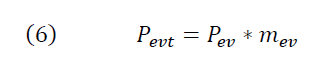
Frequency variations in a power system occur because of an imbalance between generation and load. When the frequency value of a power system reaches the emergency condition, the control strategy is initiated.
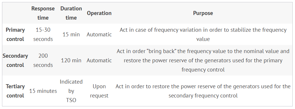
The frequency control is divided in three levels: primary, secondary and tertiary controls. Each frequency control has specific features and purposes.
Primary Control
The primary control (or frequency response control) is an automatic function and it is the fastest among the three levels, as its response period is a few seconds.
When an imbalance between generation and load occurs, the frequency of the power system changes.
For example, with a load increase, the generated power doesn’t immediately change, so the energy to compensate for this load increase arrives from the kinetic energy of the rotating generators that start decreasing the velocity (this is called the inertial response). After this moment, the speed controller (called the “governor”) of each generator acts to increase the generation power in order to recover this speed decreasing and try to clear the imbalance.
Generally, in about 30 seconds, each generation unit shall be able to generate the required additional power and then keep it for at least 15 minutes (this timing depends on the requirements of the transmission system operator, or TSO).
All the generation plants connected in the HV power system are called to supply this service, except the renewable energy source (RES) not schedulable (ie. wind, solar, biogas, hydraulic flow water), so, for this reason each generation unit shall have a dedicated and proper “reserve” power in order to accomplish this regulation when active.
The purpose of the primary regulation is to clear the unbalance between generation and loads, in order to take the system to a stable condition. This service is mandatory for all the generators entitled to provide it and not remunerated.
Regarding the not schedulable RES, these generators must be able to work with a defined P(f) function, in order to modulate their power according to the frequency value. This is easier in case of over-frequency, which requires power decrease. However, it could be really complex (almost impossible) in case of under-frequency, which would require a power increase, not always possible (even with a reserve power) due to the volatility of the primary resource itself.
The continuous growth of RES implies the reduction of thermoelectric plants in operation, with consequent difficulties to perform this frequency regulation, for the reasons explained above. There are already different solutions under analysis and some of them already in place in several power systems (battery energy storage systems are one of the most promising). This is one of the main challenges to the massive deployment of RES in the power systems.
Secondary Control
Once the primary regulation accomplished its target, the frequency value it’s different from the nominal one, the reserve margins of each generator have been used (or partially used) and also the power exchange between the interconnected power systems is different from the predefined one. So, it’s necessary to restore the nominal value of the frequency, the reserve of each generator previously used, and the power exchange among the power systems. This is the purpose of the secondary control.
In order to perform this task, there are some generators entitled to perform the secondary control, through a dedicated reserve power. This reserve depends on the requirement of each TSO and usually, it’s a percentage of the maximum power available, with a predefined minimum value to guarantee independently from the maximum power of each generator.
If the frequency value is less than the nominal one, additional generation capacity needs to be started, while if the frequency value is higher than the nominal one, some generation capacity must be stopped, or the load has to increase.
The secondary control is usually performed in an automatic way, by all the generators that participate to this regulation, through specific “set-point” sent by a central controller.
Figure 1 shows an example of the first two levels of control after a frequency event in the system. The green line and the red-dashed line show two different responses according to the inertia level of the system (power systems with low generation produced by rotating machines will have low inertia level).
Figure 1 – Example of frequency response after a frequency event. Source Scientific paper Impact of Distributed Energy Resources on Frequency Regulation of the Bulk Power System
This service is usually remunerated according to the negotiation condition in each energy service market.
Tertiary Control
After secondary control is completed, the reserve margin used for this control shall be restored too and this is the purpose of the tertiary control (or replacement reserve) the last level of frequency control. In order to perform this restoring, the TSO calls send single producers (even the ones not involved in the secondary control) the operating prescriptions related to power variation for the generators already in operation and if needed asking start-up generators not operating at that moment. This control level is not automatic but it’s executed upon request from the grid operator, and its remuneration follows the same rules of the secondary control.
A Review of the Three Regulation Levels
The table below shows a brief summary of the three regulation levels and the main features of each.
.
It is defined by the local TSO and the values can be different for each system, according to specific needs
Author: Pietro Tumino received his MSEE from the University of Catania in March 2012. His great passion for renewable energies brought him to join Enel Green Power, where he has worked since November 2015, starting at Solar Centre of Excellence in the Solar Design unit/Engineering and now as Project Engineer. He focuses on the design of photovoltaic plants, planning and coordinating photovoltaic projects in the development and execution phases. Previously he worked at Enel Distribuzione, focusing on network technology unit/remote controls and automation systems and helping the development and testing of solutions for smart grids. In his downtime, he loves football, playing guitar, and rock music.
Published by Jerzy Stanisław ZIELIŃSKI, Uniwersytet Łódzki, Kat. Informatyki
Abstract: The paper begins with a short presentation of Smart Grid (SG) being the starting element of a chain of developing the idea of “smartness” not only in power but also in all industry branches implying growth of data generation (Big Data problem). Parallel to the smart-and the big data problems, new informatics tools, such as Cloud Computing (CC) and Internet of Things (IoT) are developed. The main part of the paper describes specifics of these new tools, (e.g. Industrial Internet of Things, dew- and fog CC) and their collaboration in terms of solving the big data problem. Final remarks present the Author’s view on further development of these problems.
Streszczenie: Artykuł rozpoczyna się krótką prezentacją sieci inteligentnej zapoczątkowującej ideę „Smart” nie tylko w elektroenergetyce, ale i w innych gałęziach przemysłu, powodując zwiększenie generowania danych (problem Big Data).Równolegle z rozwojem koncepcji „Smart” i Big Data rozwijają się nowe narzędzia informatyczne, jak przetwarzanie w chmurze, Internet rzeczy. Główna część artykułu przedstawia specyfikę tych nowych narzędzi (np. przemysłowy internet rzeczy, odległe/mgliste przetwarzanie w chmurze) i ich zastosowanie w rozwiązywaniu problemu Big Data. Uwagi końcowe przedstawiają pogląd autora na dalszy na dalszy rozwój poruszonych tematów. Czy smart grids potrzebują nowych narzędzi informatycznych?
Keywords: Smart Grid, Industrial Internet of Things, Big Data, Cloud Computing Słowa kluczowe: sieci inteligentne, przemysłowy internet rzeczy, ogromne dane, przetwarzanie w chmurze
1. Introduction
The idea of Smart Grid (SG) evolved in the late 20th century as a result of blackouts in the USA and other countries [1], which facilitated the development of SG and subsequently smart- buildings, cities, industry, etc. using chip-based devices (such as Smart Meters). Each of the smart entities generates, sends, receives and stores data; according to CISCO’s prediction [2], in 2020, the number of data will be equal to 1018 , which will intensify the already growing Big Data (BD) problem.
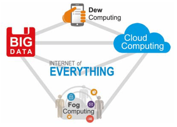
Fig.1. Examples of Big Data sources [1]
The same period Cloud Computing was a matured tool and the Internet of Things completed the stage of infancy and started gaining practical importance. According to [3], in 2015, the value of the IoT market reached $700 milliard, while the forecast for 2020 for this market foresees that this value will reach $ 1.7 billion (Cisco’s CEO has pegged the Internet of Things at a $19 trillion market). The aim of the paper is to present the current state of all of these aspects starting with the problem of Power as a very important part of information society activity and transferring the result to industry (Industrial Internet of Thing).
2. Smart Grid
According to [1] there are following characteristics of Smart Grids:
1. “It is self-healing (from power disturbance events). 2. It enables active participation by consumers in demand response. 3. It operates resiliently against both physical and cyber attacks. 4. It provides quality power that meets the twenty first century needs. 5. It accommodates all generation and storage options. 6. It enables new products, services and markets. 7. It optimizes asset utilization and operating efficiency.”
Now it has been introduced new term “Resilience” which is “…more general (including weather/climate, geomagnetic storm and power disaster and the need for forecasting) than the term self healing” [9].
Smart Grid (SG) cover all Renewable Energy Sources (RES) [4,5,6,7] available in the area of the SG activity, which has impacted and transformed the twentieth century hierarchical and natural monopoly management system into a number of dispersed, however collaborating smaller systems. This has led to an increase in the number of generated-, transmitted-, transformed- and stored data [8]. When we are considering the Power System (PS) we need to remember that for several dozen years the System Control and Data Acquisition (SCADA) has supported the Power System (PS) operation, initially being installed in transmission lines with rated voltage ≥ 220kV and now being applied in distribution (≤110kV) and even low grids. The system consists of remote terminals linked directly with sensors, measurement devices, actuators, etc.
In some countries (the USA, Japan, and Switzerland), Phasor Measurement Units (PMU) are installed to measure basic electrical parameters in the same real time in all remote nodes of the grid – these measurements are performed in the central dispatcher unit. Since the SCADA and the PMU systems deliver data important for technical operation [9] it may turn necessary to build at an individual voltage level separate sensor networks with interfaces to exchange data important for supporting management decisions in the PS. GE in California is a good example of this type of activity: “A couple of years ago, we opened a new Global Software Center headquartered in San Ramon, California, and committed $1 billion over a 3 year period to accomplish our vision for the Industrial Internet. We are developing solutions that help our customers increase productivity and reduce costs, whether they operate power plants, jet engines, or locomotives around the world” [11]. Parameters to perform simultaneous measurements in dispersed power networks are important due to the high propagation velocity of electromagnetic wave, however it will not be necessary to install the PMUs in most industrial facilities. Nevertheless the SCADA operates in some factories, which indicates that it will be possible to install additional sensors.
According to [12] it has to be remembered that power is very important, but only a part of Energy System with gas, petrol and another liquid fuel, steam and hot water etc. which in future would more effectively collaborate, which indicates that an additional source of a huge quantity of data will be necessary.
There are numerous common occasions where these two systems (electricity and gas) have to collaborate, e.g. in the CHP, on the market (where each system can have different businesses targets). Nevertheless both these systems are grid-based, and it is important to investigate common solutions, for instance in the field of the ICT (mobile) automation and management. Application of gas in the power production can provide such significant benefits as high efficiency, flexibility and reliability, low gas emission, etc. Unfortunately, there are certain barriers to using this fuel for the purpose of power production, and they include high costs and unstable import conditions in Poland [12]. One can find publications on research in the area of gas and electricity collaboration, e.g. [11,14,15,16,18,20]. It has to be stressed that gas application involves the problem relating to its explosive properties; a case study of [12] addresses this problem. In order to apply IoT in both systems it will be necessary to build two independent sensor networks due to different key control-related parameters and different velocity between the electromagnetic wave and the gas flow. It will be necessary to apply an interface to exchange data between these two systems.
3. Internet of Things (IoT)
A global infrastructure for the information society, enabling advanced services by interconnecting (physical or virtual) things based on existing interoperable information and communication technologies is called Internet of Things (IoT) by Vermesan and Friess [21]. These authors, as well as the IERC, stated that IoT is “A dynamic global network infrastructure with self-configuring capabilities based on standard and interoperable communication protocols where physical and virtual “things” have identities, physical attributes, and virtual personalities and use intelligent interfaces, and are seamlessly integrated into the information network”. The Digital Agenda for Europe [22] has introduced the following explanation: “Internet of Things (IoT) is a technology and a market development base on the interconnection of everyday objects among themselves and applications. IoT will enable an ecosystem of smart applications and services, which will improve and simplify EU citizens’ lives.” [8]. Studying bibliography one can find many Internet of…, e.g. Internet of Everything (IoE), Internet of Service (IoS), Web of Things (WoT), etc. We will consider only three interesting cases: Industrial Internet of Things (IIoT) Narrowband IoT (NB-IoT) and Internet of Bio- Nano Things [23].
Industrial Internet of Things (IIoT) [24] “… is connecting the physical world of sensors, devices and machines with the Internet and, by applying deep analytics through software, is turning massive data into powerful new insight and intelligence. We are entering an era of profound transformation as the digital world is maximizing the efficiency of our most critical physical assets. Cisco’s CEO has pegged the Internet of Things at a $19 trillion market. The IIoT is a significant sub-segment and includes the digital oilfield, advanced manufacturing, grid automation, and smart cities. We are experiencing incredible innovation around the Internet as it accelerates the connection of objects not only with humans but also with other objects. Every Industry will change. The Industrial Internet of Things (IIoT) is truly the next significant wave of technology adoption in global industrial markets. Armed with data from volumes of sensors and intelligent machines, software analytics will drive efficiency.
Another solution supporting IIoT and especially a wireless application of IoT is Narrowband IoT (NB-IoT). (Technology LTE Car NB1 Release 13, approved in June 2016 by 3GPP (organization defining wireless communication) [25]. This tool is very useful in sending data to Cloud Computing using Fog- or Dew Cloud Computing (see paragraph 4) optimization.
When considering IoE in the macroscale environment, it is worth mentioning its development in nanoscale, i.e. Internet of Bio-Nano Things (IoBNT) [23]. A group of professors from the USA and Finland [23] introduced the idea of IoBNT in their investigations inspired by this concept, in which they tested a nanomaterial (graphen) as a nano technological tool that has enabled to build biologically embedded computer devices developing networks inside the body to control activity of toxic agents and wastes. “Human Neuro-Activity For Securing Body Area Networks: Application of Brain Computer Interfaces To People-Centric Internet Of Things” [20] is another interesting IoT application in the human body.
The lack of standards is one of the key barriers in the practical (IIoT) application [26]. The IEEE Communication Committee considers solutions to the problem, and results of this Committee’s work are published in the Communications Standards – a Supplement to the IEEE Communications Magazine.
4. Cloud Computing, Big Data and Cybersecurity
The need to save expenses on hardware has stimulated the development of Cloud Computing (CC). Bibliography, e.g. [27], contains a lot of information on specific characteristics of CC as well as on its practical use. The growing number of generated data and the need for its storage, processing, etc. imply the use of CC, however at the same time it generates the following problem: where a data source is distant from CC, the so-called “edge computing” problem arises [27] due to the transmission of this data that requires many transmission channels. As a result, this solution is not feasible due to its cost. To resolve this problem, one of the following approaches can be used: FOG Computing [2] or Dew Computing [29]. Both proposals use the same logic method: process data in the location where it is generated and provide CC only with these results that are necessary for other users.
Fig.2. Paths to Cloud Computing [1]
The bibliography contains the following two approaches in terms of BD considerations: Under the first approach, BD is perceived as “analytical workloads that are associated with some combination of data volume, data velocity and data variety that may include complex analytics and complex data types“ [30] while the other perceives BD as data volumes necessary to filter, store, transform to practical use in place of their generation and, if necessary, send some part to cloud [31].
Big Data growing exponentially can be illustrated by a number of wireless devices going to grow from 2015 to 2020 from 10 billion to 40 billion, and John Chalmers (CISCO Systems chairman) predicts that the IoT will grow to be a $19 trillion global market (“the GDP of the entire world is currently just a little more than $100 trillion”) [3]. It implies the need to protect data against cyberattacks. “Chris Bronk, a cybersecurity expert and professor of computer and information systems, perceives cybersecurity as one of the fastest growing industries in the world” [3].
5. Informatics Tools and SG
Informatics tools consists of two main groups: hardware with devices containing integrating circuits (IC) and software with a big number of programs written in different languages necessary for operation of IC devices. It means that SG using SCADA and/or PMU use informatics tools from both groups controlling power systems (PS).
In this context we should now consider whether IoT/IoE or CC could be used as new soft informatics tools from the SG point of view.
Due to a high velocity of the electromagnetic wave (order velocity of light) SG cannot use CC to control PS. As a result of application of SCADA and/or PMU, SG supports sensor networks which will be able to collaborate based on detailed comparison of sensor parameters and functions in both sensor networks (Fig. 1); as a result of these comparisons application of interfaces might turn necessary.
6. Final remarks
The above considerations present results of researches and practical solutions developed recently, however we have also taken into account intensive researches supported by tests in real environment, new products enabling new solutions in many areas as well as more accurate prediction. For example in paragraph 2 we discussed a change in management systems in power from traditional hierarchical to dispersed, whereas in May “A Hierarchical EMS for Aggregated BESSs in Energy and Performance-Based Regulation Markets” [32] was published (BESS means battery energy storage systems installed in power systems as a result of development of renewable energy sources). Also in May another paper presenting “Distributed Generation Monitoring for Hierarchical Control Applications in Smart Microgrids” [33] was published. Another power-related problem has been considered in the paper entitled “A Robust Linear Approach for Offering Strategy of a Hybrid Electric Energy Company” [34] (Hybrid means that company has both energy generation and energy retailing businesses. In my opinion this approach can be considered as a kind of Transactive energy solution [32]). “Multi-Linear Probabilistic Energy Flow Analysis of Integrated Electrical and Natural-Gas System s”is an example of the paper that considers common solving problem in electric and gas system.
The above mentioned cases must be considered before trying to apply any of the above-mentioned new methods. This is likely to provide a new insight into contemporary solutions.
The author wishes to thank Mr Piotr Czerwonka, PhD, for his support in editing the work.
REFERENCES
1. Zieliński JS. (2017) New Informatics Tools in Data Management, The Xth SIGSAND/PLAYS EuroSymposium’2017. 2. CISCO WHITE PAPER: FOG Computing and the Internet of Things: Extend the Cloud to Where the Things Are. Access 06.05.2017. 3. Ross A.: The Industries of Future. Simon & Schuster, 2016, 4. Hatziargyriou N. (Ed) (2014) Microgrids.. Architecture and Controls. Wiley, IEEE Press, 2014. 5. Matusiak B., Zieliński JS. (2011) Renewable Energy Sources Intrusion into Smart Grids – Selected Problems. Przegląd Elektrotechniczny 9a/2011, . 206-209. 6. Matusiak B.E, Zieliński JS. (2014) Internet of Things in Smart Grid Environment. :Rynek Energii 3/(112)-2014, . 115-119. 7. Zieliński JS. (2012) Smart Distribution Grids Importance in SG Development. Rynek Energii, 1/2012, 179-182. 8. Zieliński JS. (2015) Internet of Everything (IoE) in Smart Grid. Przegląd Elektrotechniczny 3/2015, pp. 157-159 9. Zielinski J.S.: Microgrids and Resilience. Rynek Energii 2/216, 108-110 10. Bush S.E. (2014), Smart Grid. Wiley, IEEE Press 11. Xu X., Jia H., Chiang H.-D., Yu D.C., Wang D.: Dynamic Modeling and Interaction of Hybrid Natural Gas and Electricity Supply System in Microgrid. IEEE Transactions on Power Systems vol.30 No.3 2015. pp 1212-1221. 12. Case Study Electromagnetic Interference Between Transmission Lines nd Buried Pipelines. POWERSYS marketing@powersys.fr Access 11.02.2016 13. Bućko P.: Perspektywy wykorzystania gazu ziemnego do produkcji energii elektrycznej w Polsce. Rynek Energii 3/2015, 17-22. 14. Chen S., We Z., Sun G., Cheung K.W., Sun Y.: Multi-Linear Probabilistic Energy Flow Analysis of Integrated Electrical and Natural-Gas System. IEEE Transactions on Power Systems vol. 32 No. 3, May 2017, 1970-1979. 15. Gil M., Dueňas P., Reneses P.: Electricity and Natural Gas Interdependency: of Comparison of Two Methodologies for Coupling Large Market Models Within the European Regulatory Framework. PWRS vol.31 No.1. January 2016, pp 361- 16. Meegahapola L., Flynn D.: Characterization of Gas Turbine Lean Blowout During Frequency Excursion in Power Networks. IEEE Transactions on Power Systems vol. 30, No. 4, July 2015. 1877-2997 17. Qiu J.,Yang Dong Z., Zhao J.H., Xu Y.,Zheng Y., Li Ch., Wong K.P.: Multi-Stage Flexible Expansion Co-Planning Under Uncertainties in a Combined Electricity and Gas Market. IEEE Transactions on Power Systems, vol. 30 No. 4, July 2015, 2119-2129. 18. Zhang X., Shahidehpour M., Albfulwahab A., Abusorrah A.; Hourly Electricity Demand Response in the Stochastic-Day-Ahead Scheduling Of Coordinated Electricity and Natural Gas Networks / IEEE Transactions on Power Systems vol. 31,No. 1, January 2016, pp 592-600. 19. Valenzuela-Valdes J. F., Angel López M.,, Padilla P., Padilla J.L, Minguillon J. Human Neuro-Activity For Securing Body Area Networks: Application of Brain-Computer Interfaces To People-Centric Internet Of Things. C. Feb 2017,62-67. 20. Vermesan O., Friess P. (2014) Internet of Things – From Research and Innovation to Market Deployment. River Publishers, Denmark 21. Akyildiz I.F., Pierobon M., Balasubramanian S., Koucheriavy Y.: The Internet of Bio-Nano Thing. CS March 2015, 32-40. 22. Communication Standards. September2015, December 2015, September 2016. A Supplement to IEEE Communication Magazines. 23. Czerwonka P.(2016) Zastosowanie chmury obliczeniowej w polskich organizacjach. Biblioteka, Łódź 24. Hao H., Corbin ChD. Kalsi K., Pratt R. (2017), Transactive Control of Commercial Buildings for Demand Response. IEEE Transactions on Power Systems vol.32 No.1 January 2017, pp 774-783. 25. Kazemi M., Zareipour H., Ehsan M, Rosehartr WE.D.: A Robust Linear Approach for Offering Strategy of a Hybrid Electric Company. IEEE Transactions on Power Systems vol. 32 No. 3, May 2017, 1940-1959 26. Olszak C.M., Mach-Król M., Big Data: How to Gain Value for Organizations. In: M. Themistocleous, V. Morabito, A. Ghoneim (Eds.), Online Proceedings of the 13th European Mediterranean & Middle Eastern Conference on Information Systems (EMCIS), , p. 7-15. 2016, Kraków, Poland. ISBN 978-960-6897-09-2. 27. Rindos A., Wang Y.: Dew Computing: the Complimentary Piece of Cloud Computing, @016 IEEE International Conferences on Big Data and Cloud Computing (BDCloud),Social Computing and Networking (SocialCom),Sustainable Computing and Communication(SustainCom). DOI 10.1109BDCloud-SocialCom-SustainCom.2016.14 28. Ross A.: The Industries of Future. Simon & Schuster, 2016, 29. Seyedi Y., Karimi H. Grijalva S.: Distributed Generaion Monitoring for Hierarchical Control Applications in Smart Microgrids. IEEE Transactions on Power Systemsvol. 32 No.3#, May 2017, 2305 -2314. 30. Sun X., Ansan N.: EdgeIoT: Mobile Edge Computing for the Internet of Thing. IEEE Communications Magazine December 2016, pp 22- 31. Zhang T., Chen S.X., Gooi H.B., Maciejowski J.M.: A Hierarchical EMS for Aggregated BESS in Energy and Performance Base Population Markets. IEEE Transactions on Power Systems vol. 32 No. 3, May 2017, 1751-1781. 32. Zieliński JS. (2017) Transactive Energy and Internet of Everything. Rynek Energii 2/2017 pp. 92-94. 33. Zieliński JS. (2017) New Informatics Tools in Data Management (in preparation) 34. http://di.com.pl/nb-iot-nowe-możliwosci-i-wyzwania-interneturzeczy-57114 35. JEFF-DORSCH: Where are The IoT Industry Standards?http://semiengineering.com/where-are-the-iot-industrystandards/accesss 2016-10-11 36. McRock: Industrial Internet of Things. Access 21.05.2017.
Author. Prof. dr hab. inż. Jerzy Stanisław Zieliński, Uniwersytet Łódzki, Wydz. Zarządzania, Katedra Informatyki. E-mail: jzielinski@wzmail.uni.lodz.pl
Source & Publisher Item Identifier: PRZEGLĄD ELEKTROTECHNICZNY, ISSN 0033-2097, R. 94 NR 4/2018. doi:10.15199/48.2018.04.08
Published by Andrzej ŁEBKOWSKI, Gdynia Maritime University, Department of Ship Automation
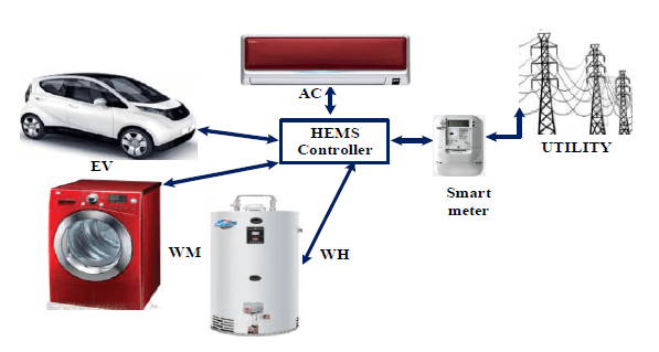
Abstract. Electric vehicles (EVs) emerged as a next step in the evolution of transport technology. The article describes structure of system used for optimal management and monitoring of electric vehicle parameters, especially in regions of low possible ambient temperature. System can be used in all types of electric vehicles, such as: cars, ATVs, motorbikes, scooters, bicycles or boats. Application of GSM/GPS technologies allows remote monitoring of state and management of vehicle battery thermal aids (increasing battery performance and longevity while reducing operating costs) as well as control of vehicle to grid and grid to vehicle energy flow in smart grid systems. System functions were tested on an electric vehicle in normal road conditions at a period of ambient temperature reaching -25°C (-13°F). Article contains road tests results along with comments on possible benefits that may be derived from the application of the system in practice. (System zarządzania pakietem akumulatorów w pojeździe z napędem elektrycznym).
Streszczenie. Pojazdy elektryczne stanowią następny krok w ewolucji technologii transportu. Artykuł przedstawia strukturę systemu do optymalnego zarządzania i monitorowania parametrów pojazdu elektrycznego, szczególnie w warunkach niskiej temperatury otoczenia. Typy obsługiwanych pojazdów obejmują samochody, quady, motocykle, skutery, rowery elektryczne oraz łodzie. Zastosowanie technologii GSM i GPS umożliwia zdalny monitoring i zarządzanie modułem ogrzewania akumulatorów a także kontrolę przepływu energii z sieci do baterii I baterii do sieci (smart grid). Funkcje systemu zostały przetestowane w warunkach drogowych przy temperaturach dochodzących do -25°C. Artykuł zawiera wyniki badań wraz z omówieniem potencjalnych korzyści wynikających z zastosowania opisanego systemu.
Słowa kluczowe: pojazdy elektryczne, system zarządzania akumulatorami, akumulatory litowe, termiczne kondycjonowanie akumulatorów Keywords: electric vehicles (EV), battery management systems (BMS), lithium batteries (Li-Ion, LiFePO4, LTO), thermal management
Introduction
Car sales statistics show, that there is a growing trend in sale of vehicles having electric propulsion [1-3]. The reasons of this behavior are undoubtedly the advantages of using such a vehicle: decreased energy consumption, limited noise emission, lower operating costs, social prestige. Additionally, regulations in certain countries can influence owners to buy this specific car variety, by virtue of: motor insurance discounts, free of charge motorways and parkings in city centres, access to separate bus-lanes, possibility of free battery recharging in public charge stations. The main factors influencing purchase decision are ecology and economy of use. Customers have a wide choice of vehicles offered by reputable dealer networks or by less known makes, as well as a possibility of conversion of internal combustion engine car to electric propulsion either by themselves or in specialized car shops. No matter which choice, users of such vehicles want to have full control over it, i.e. know whether the battery is charged, if the vehicle can or cannot be used (for example due to bad battery condition or malfunction of some component).
This paper tries to present a system to manage an electric vehicle being it a car, an ATV, a motorbike, a scooter, a bicycle or a boat. Application of Management System for Electric Vehicle – (MSEV) can greatly improve the electric vehicle battery performance. Its impact can be highest in vehicles operating during low ambient temperature conditions, when outside air temperature drops below 0°C (32°F). While the individual cells in the electric vehicle are cold, and their temperature is less than 0°C (32°F), they can be easily damaged. Additionally, their performance suffers as the temperature drops [5-7]. The phenomena of battery longevity, performance and efficiency decrease as a function of dropping temperature are well known and were the subject of many articles.
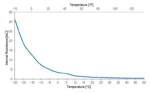
The probability of cell damage is the greater, the ambient temperature is lower (Fig.1). The vehicle range is also becoming severely limited. Electric vehicle users accustomed to driving every day, during cold periods of ambient temperature 0°C (32°F) or lower will, at first, notice the reduced reading of on-board potential range gauges. Only after the self-heating process takes place due to battery discharge, the temperature inside the battery will raise to nominal value. The operation of such vehicle should take place with battery temperature (previously chilled by the cold environment) at nominal value, while this temperature will be achieved probably when the vehicle and its user have reached the destination. If the vehicle two-way charger will not be plugged-in, the battery’s temperature will again drop to low temperature of the surrounding air.
Fig.1. The dependence the internal resistance of the temperature for LiFePO4 [4]
Another important matter is that charging a battery in low temperature conditions limits its ability to absorb electric charge. Charging any cold battery severely limits its operating life, including lithium batteries in which the low temperature aging mechanism caused by lithium buildup on negative electrode is present. This mechanism, along with low temperature and a vehicle not fitted with battery heating system suggests a need to reduce the setting of BMS system charging voltage to a lower value, thus allowing the two-way charger to proceed without greatly reducing the battery’s State Of Health (SOH) (e.g. as recommended in [4,8] 0,25C, 3,55V for LiFePO4 cells). During the tests conducted by the author it was observed that when the ambient temperature was below 0°C (32°F), the battery’s ability to supply energy became limited. During operation in said conditions, a considerable voltage drop is observed when the battery is loaded. When the voltage drop under load exceeds 2V, in case of LiFePO4 cell, while its nominal value is about 3.2V, the irreversible chantestinge in electrochemical internal structure of the cell takes place which results in permanent micro-damage. This phenomenon can be compared to a fuel tank with a small hole, through which the fuel seeps out. In the case of a battery, the low temperature combined with high load causes micro-damage. The cell’s internal resistance is increasing which reduces State Of Health (SOH) and State Of Charge (SOC) [9-12]. The solution would be to install a battery heating system, which consumes a relatively small amount of electrical energy in relation to the benefits such as better battery efficiency translating into better vehicle range and greater available power from the drivetrain. Such a system, combined GSM/GPS monitoring system (Fig.2) can provide very efficient battery electric vehicle operation.
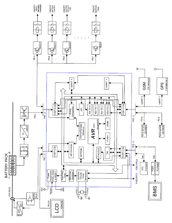
Fig.2. Structure of an Management System for Electric Vehicle
Using GSM/GPS technology, the user can monitor the state of battery at any moment, as well as control its operation e.g. turn on the charging process or turn on the heating system. Additionally, thanks to simple and inexpensive heating elements the system can be applied to virtually every electric vehicle containing a battery. Components of MSEV using elements of AI (Artificial Intelligence) processing, such as fuzzy logic or expert system database can influence optimal utilization of battery electric vehicle in low ambient temperature conditions.
The system can for example check the weather forecast and, if the forecast reports possible temperature drop, it can then request the user to plug in the vehicle to charging socket. Depending on the outside temperature the MSEV can in the first place heat up the battery pack and then commence its charging. With the charging finished, it can proceed according to program defined by the user – either maintain the pack’s temperature at the level which enables driving, or preheat the battery to be ready to drive at the selected time. The scope of work and MSEV research results presented in this paper have demonstrated its usefulness and validity of its use in battery electric vehicles in which the manufacturer did not anticipate battery heating, especially if the vehicle is operated in geographic regions with ambient temperatures often less than 0°C (32°F). System testing was conducted in real driving conditions on Fiat Panda electric vehicles built in Gdynia Maritime University (Fig.3).
While the MSEV was tested in cars, its simple design and available functions allows it to be used in any electric vehicle, be it a motorbike, an ATV, a scooter, a bicycle or a boat.
Fig.3. The tested car Fiat Panda EV in winter conditions
MSEV functions
Postulated Management System for Electric Vehicle – (MSEV) can be used for mass produced vehicles, as well as for small-lot produced and converted from ICE propulsion.
Selection of possible system functions depends only on what the user will want to manage and monitor. MSEV can be used for remote monitoring, alarming and diagnostics of each vehicle component and for logging of any parameters using GSM/GPS technology through any cell phone using SMS messages. Applied technical means allow the user to read out the battery pack parameters or to control the operation of the two-way charger. The user can configure the system to send him an SMS with vehicle parameters to a predefined phone number. The main point of this technical solution is to fulfill goals including:
• monitoring of parameters vital from the perspective of its user,
• remote control of subsystems e.g.: battery charging system compatible with smart grids (V2G – vehicle to grid mode, G2V – grid to vehicle mode), battery heating system, cabin heating system,
• alarming (SMS on mobile), in case of exceeding nominal value of parameters e.g.: main battery Depth of Discharge (DOD), auxiliary 12V battery DOD, high/low battery temperature,
• requesting the user to take some action e.g. request for plugging in the vehicle to the power grid after checking the weather forecast in order to power the battery heating system,
• alarming in case of attempted access by unauthorized persons or burglary,
• widely understood diagnostics associated with the estimation of individual parameters from measured signals,
• logging of vehicle components’ parameters, • logging of vehicle location and motion parameters, • remote monitoring of vehicle and it’s components parameters and operation.
MSEV finds use in acquisition of many parameters describing state of an electric vehicle. Application of GSM/GPS technology allows remote monitoring of these parameters and remote control of executive and measurement modules of the vehicle. The main part of MSEV is a Central Processing Unit (CPU) containing microprocessor controlling vehicle parameters, supplied from on board 12V power. CPU gathers signals from various onboard sensors: battery voltage sensor, battery charge current sensor, motor supply current sensor, auxiliary supply current sensor, motor temperature sensor, battery temperature sensor, ambient temperature sensor, vehicle speed and distance traveled sensor, accelerometers and gyros, door switches and other anti-burglary sensors. It can also request the driver to input the approximate distance he is planning to travel, and ask the driver’s permission to become a part of a smart grid. The CPU also communicates with internal GSM and GPS modules, internal self-diagnostic module and has backup power system. Additionally, the MSEV CPU communicates with other vehicle components, including: two-way charger control block, main battery heating system, user interface (including remote monitoring), data recording device (flash card, USB flash drive, etc.), OBD-II or similar external diagnostic system, emergency power system, additional traction battery/power source (range extender).
The MSEV contains large scale of integration electronic components and easy to install sensors and modules. The optimal use of electric vehicle is possible, thanks to sensors, executive/measurement modules, reference values for each vehicle parameters stored in internal database and artificial intelligence contained within device programming and via cooperation with vehicle subsystems.
This cooperation can lead especially to:
• proper operation of main traction battery through automatic and maintenance-free control of vehicle two-way charger,
• logging of all measured parameters,
• estimation of vehicle parameters, like: amount of energy in main battery, vehicle range, etc.,
• informing the user about vehicle state through user interface and GSM communication module,
• informing the user about distance and location of closest charging station,
• monitoring the state of main battery and control of systems prolonging its useful life, like cooling or heating systems,
• possibility of remotely informing the user about the vehicle whereabouts and its parameters (voltages, currents, temperatures, SOC, etc.),
• possibility of asking the user to perform some action e.g. requesting plugging in the vehicle to the power socket after checking the weather forecast in order to power the battery heating system,
• possibility of changing the BMS settings depending of battery pack temperature,
• feature of turning on the two-way charger during the night, when the electricity price is much lower (for example between 10 PM and 6 AM),
• possibility of smart grid integration – using the vehicle battery as an electrical grid energy buffer,
• warning the user in case of vehicle malfunction or fire hazard.
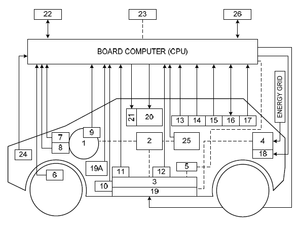
MSEV structure
MSEV structure is presented on figure 4 showing block diagram embedded in vehicle side silhouette view. MSEV contains on board microprocessor CPU, which can communicate with vehicle user through user interface and with external systems for diagnosis and log download through external port. Using data from on board sensors and devices: distance travelled and speed sensor, traction motor voltage sensor, traction motor current sensor, traction motor temperature sensor, battery pack temperature sensor, battery pack voltage sensor, ambient temperature sensor, extender (additional battery pack or power generator) it is possible to estimate the remaining power in main battery. Additionally, data from sensors: distance travelled and speed sensor, traction motor voltage sensor, traction motor current sensor, traction motor temperature sensor, battery pack temperature sensor, battery pack voltage sensor, battery pack charging current sensor, ambient temperature sensor, range extender (additional battery pack or power generator) (Fig.4) allows estimation of remaining vehicle range. The vehicle range is estimated from the current reading by the current sensor located on the power wiring supplying the onboard devices and drivetrain, and by the temperature reading of battery pack reported by temperature sensor.
Fig.4. The structure of Management System for Electric Vehicle (MSEV).
1. vehicle traction motor/motors, 2. power inverter (DC/AC, DC/DC), 3. electrical energy reservoir (battery pack), 4. two-way charger, 5. 12VDC power supply (12V battery or DC/DC inverter), 6. distance travelled and speed sensor, 7. traction motor voltage sensor, 8. traction motor current sensor, 9. traction motor temperature sensor, 10. battery pack temperature sensor, 11. battery pack voltage sensor, 12. battery pack charging current sensor, 13. angular acceleration sensor (gyro), 14. accelerometer sensor, 15. GPS module, 16. GSM module, 17. ambient temperature sensor, 18. on board two-way charger control system, 19. battery pack with heating/cooling module, 19A. vehicle cabin heating/cooling module, 20. user communication interface, 21. communication port for parameters recording (SD card, USB, etc.), 22. communication interface for external devices (PC, external database, etc.), 23. power supply system, 24. door switches and anti-burglary sensors,25. range extender (additional battery pack or power generator), 26. self-diagnostic module
The CPU processes data from the above mentioned sensors so it can warn the user, using the user interface, about exceeding the value of critical vehicle parameters including: low voltage of main battery, motor overcurrent, low vehicle range due to low remaining charge in main battery, as well as inform the user about the state of all parameters measured by and estimated from sensor data including total distance travelled since system installation, distance travelled since last charge, distance possible to travel using energy remaining in main battery and additional power source. CPU can also indicate the distance and whereabouts of closest charging station using internal location database.
The MSEV can, using the GSM module, alert the user remotely about exceeding critical parameter values, such as: low voltage of main battery, low vehicle range due to low remaining charge in main battery, exceeding operational parameter values e.g. motor overcurrent, vehicle overspeed, vehicle operation outside of designated area. Besides transmitting parameter values it is possible to monitor the state of all vehicle components using internal vehicle network. User can access the parameters of devices including motor controller, two-way charger, Battery Management System including individual cell data (voltages, temperatures), battery heating system, cabin heating system, power braking system, etc.
The CPU computer board consists of an Atmel Atmega324PA microcontroller and peripheral devices including: GPS module FGPMMOSL3, GSM module ZTE MG3030, real-time clock PCF8583, serial port expander PCA9555D, analog switches ADG707, voltage to frequency converter LM331, operational amplifier LM358D, isolating DC/DC converters type AM1D, relays, Dallas temperature sensors type DS18B20, HD44780 compatible alphanumeric LCD module, and numerous passive devices. The part of computer board structure responsible for conditioning the battery pack is presented in figure 5.
Fig.5. The simplified computer board structure
Application of external electronic modules such as GSM modem, GPS module or RTC clock requires use of hardware communication busses. The chosen microcontroller contains all required serial busses. The project uses USART interface to communicate with GSM modem and GPS module and two wire TWI interface to communicate with RTC clock chip.
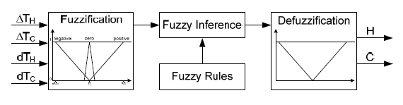
Artificial Intelligence methods, such as fuzzy logic, used in the MSEV are used mostly in conjunction with the battery pack temperature control process. Usefulness of these methods in control applications using a microcontroller was proven in [13-15]. Because a fuzzy logic temperature controller is not a topic of this paper, it will be presented very briefly. During the non-linear process of electric vehicle battery pack temperature control, there are 2 input variables, for a system with only battery heating, or 3 input variables, for a system with both battery heating and cooling. In a “heating only” system, these variables are: the difference between the setpoint temperature of the battery pack, to which is should be heated and its real temperature – a mean of two battery packs temperatures ΔTH (ΔTH = THset – Tactual) and derivative of this difference dTH. In a system with both heating and cooling, these variables are: a difference between setpoint heating temperature of the battery pack and its real temperature – a mean of two battery packs temperatures ΔTH, a difference between setpoint temperature to which the battery pack should be cooled and its real temperature (a mean of two battery packs temperatures) ΔTC (ΔTC = – (TCset – Tactual)) and a derivative of temperature difference dTC. The output variables of fuzzy temperature regulator are called H (Heating) and C (Cooling), they control respectively the duty cycle of the heating mats transistor (battery pack heating) and the battery pack cooling system transistor (controlling e.g.: a fan, a Peltier Cooling Module, a liquid cooling system). The complete algorithm consists of only three main steps: fuzzification of input variables, inference, and defuzzification.
The first step is implemented in fuzzification block, its goal is to evaluate and transfer the information from the quantity domain (difference of setpoint and real temperature ΔT of two battery packs) into the quality domain as a mapping of given variable into available fuzzy sets (Fig.6). The next step (inference) is an operation of deciding on inclusion of given variable into given fuzzy set, based on rules input by an expert into the inference database. The inference is based on simple IF-AND-THEN rules. IF (ΔTL is Neg.) AND (dTH is Neg.) THEN (C is Negative) The last step of fuzzy regulator operation (defuzzification) is to define a crisp value of output variable H or C, defining the operating time of heating mats or cooling system, which is correct from the point of view of input variables ΔTH or ΔTC and corresponding changes dTH or dTH. In the system in question overshoot in set temperature does not create negative consequences, because higher temperature in the given range has a positive effect on the battery pack operation. The structure of a fuzzy logic battery pack temperature controller using a microcontroller is very simple, which allows its easy implementation and reliable operation.
Fig.6. Fuzzy logic system controlling battery pack temperature
The elements of artificial intelligence that were used in the design are meant to provide optimal operation of the electric vehicle (such as: charging the battery pack in an optimal way, with the lowest grid electricity cost, and at a best possible temperature). Applied algorithms governing the operation of the battery pack are equipped with elements of artificial intelligence, such as cognitive system supporting the operation of the electric vehicle.
Fig.7. Location of battery packs in the tested car
The task of the cognitive system is to support optimal utilization of the battery pack based on the conditions stored in the knowledge base of the system, e.g. time of day in which electricity is at lower price, the time bounds on allowed smart operation, or vehicle’s user behavior e.g. determination that user usually drives the vehicle between 6:00-8:00 AM and 4:00-6:00 PM on weekdays and between 10 AM and 4 PM on weekends. The cognitive database can be modified by the user according to his preferences and habits. It gives the smart grid system operators knowledge, if and when the particular vehicle can become a part of a smart grid. The system is designed in order to maximally simplify the operation with the smart grid, and the only driver’s task is to physically connect the vehicle into the wall socket. The intelligent algorithms will allow, apart from a regular charging mode, an automatic mode where the charging would only take place in periods when the electricity price is lowest. The algorithm would also take care of the battery health and maximize its life span. These goals would be met by application of procedures allowing the charging process only when the circumstances will be optimal. By optimal, meaning: the proper future temperature of the battery, based on weather forecast data, the time of charging depending on the defined periods of vehicle operation during the day. The battery two-way charger plays a significant role in the system, as it need the capacity for two-way energy flow – from the grid to the battery during charging mode (G2V) and from the battery to the grid during the smart grid buffer mode (V2G).
The mobile application will allow the user to define the level of energy to remain in the battery in a given day at a given time. The energy level impacts directly the achievable range in particular conditions (geographic location, weather conditions). The cognitive system algorithms shall choose the operational parameters in an optimal way – by minimizing the battery Depth of Discharge (DOD) and maximizing the State of Health (SOH), by maximizing the financial gains from the trade of energy with the smart grid, maximizing the user’s own priorities (e.g. powering his own buildings in the first place).
The MSEV system is designed to create a synergy effect in a whole group of electric vehicles operating at a given region, creating and intelligent network of fully electric vehicles (EV), plug-in hybrid electric vehicles (PHEV), and fuel cell electric vehicles (FCEV).
Experimental – MSEV road tests
Due to the fact, that a smart grid monitoring station which would globally manage the energy flow has not yet been created, the MSEV could not use the smart grid functions of V2G mode and they have not been included in the tests. The testing however included the battery heating system, and it have been tested on a FIAT PANDA EV vehicle. Several such vehicles were built in Gdynia Maritime University (please refer to website at http://evpl.pl). The tested vehicle uses LiFePO4 cells and synchronous AC motor. The vehicle’s top range is about 160km (100 miles) and top speed is 170 km/h (105 mph). Testing was conducted for a period of 3 years (about 1100 trips) in normal road conditions [16,17].
The tested vehicle had two LiFePO4 battery containers with heating system. Containers were made from sheet steel, one was located in the front of the car, under the hood while the other was located in the rear, below the trunk floor. The location of both containers is presented in figure 7.
Heating units with a combined power of about 400W were installed under the battery packs as heating mats made with heating cables laid out on a rubber base. Next, the heating cables were potted in thermally conductive rubber compound, with the heat flux conductivity of about 1,6W/m∙K. Such prepared mats were located on the bottom of battery containers as shown in figure 8.
The advantage of the proposed solution in relation to systems with liquid battery pack temperature control is its simple design. As stated in the introduction, this system can be used in all kinds of vehicles in which the manufacturer did not plan any battery heating system. It can be argued, whether such system can compete with liquid based systems which allow both heating and cooling of battery packs. The performed research of MSEV have proven that for geographical regions where large drops of temperature occur in the winter meaning periods of temperature below 0°C (32°F), and the temperature during the summer not exceeding 35°C (95°F), the MSEV performs adequately allowing the vehicle to achieve higher range in low ambient temperature conditions than without such a system.
Fig.8. Heated battery container arrangement
During the tests in the summer, when the air temperature had reached 35°C (95°F), the battery pack’s maximal temperature was on the order of 50°C (122°F), which is a safe maximal value for LiFePO4 cells.
During the tests the installation of battery container cooling system based on Peltier effect modules (surface mounted) was considered, but it was eventually ruled unnecessary.
Plot of vehicle range of heating mats were also tested, the first where they were placed around the batteries instead of on the bottom, and another one where the heating cable was wrapped around the batteries without any potting compound. The most beneficial results of reheating the batteries were obtained for mats made of heating cables potted in thermally conductive rubber compound, arranged under the batteries.
Data on the battery pack temperature is gathered from several temperature sensors located in the battery container. Because the heating cable is a resistive-type electrical load it is possible to supply it either from the batteries itself, or from the mains supply after plugging in. This feature enables the battery heating system to perform with no losses in comparison to liquid systems where the flow of the coolant is circulated by pumps requiring additional electric power. Additionally, liquid based systems consume greater volume than heating cables, their design is generally much more complicated and they contain more failure-prone elements. Their mass is greater, they require periodic maintenance and service (checking the coolant level and topping off) too. They are also vulnerable to mechanical damage which can lead to leaks and loss of coolant in the circuit. The alternative is to use the internal heating methods using alternating current [18].
The best solution for a battery electric vehicle would be to use batteries which would be truly low temperature proof [19], safe in general use, fast to charge and having an energy density of at least 1000 Wh/kg. Presently available lithium batteries e.g. LiFePO4 have energy density of about 95 Wh/kg, Li-Ion 85Wh/kg, and upcoming LTO cells have 160 Wh/kg. The most important advantage of postulated solution is that MSEV contains battery temperature control module with possibility of active heating.
Optimal temperature range for use of Li-Ion battery lies between 15-35°C (59-95°F). For LiFePO4 battery the optimal temperature range of is slightly wider (Fig.1) [4].
The most important matter influencing long battery service life (the largest possible cycle count) is the voltage range between charge and discharge. Basing on data from road tests, it can be concluded that the maximal life of LiFePO4 cells can be reached at single cell voltage range between 2.80-3.65V. Furthermore, the terrain in which the vehicle is operating (hills or flat) has also its effect on the number of battery cycles. Shorter operating life is also expected in vehicles operated in sporty – aggressive driving style, associated with frequent acceleration and hard braking. Finally, the charging current and the used BMS type (active, passive) are affecting the number of cycles. The best results come with the use of active BMS and charging current no higher than 0.5C.
If the vehicle is used in region where ambient temperature during winter drops to no less than 10°C (50°F) for short periods, the user practically will not feel much of a difference in the range achieved by his vehicle. In regions with more severe winter temperatures of -20°C (-4°F), the use of electric vehicle becomes troublesome because range becomes limited to about 40-50% of nominal.
Decrease in range comes not from the use of cabin heating, which depending on the particular vehicle consumes from 0.2kW up to 4kW, but rather from the physicochemical processes taking place in the battery at low temperatures. Likewise, battery temperature higher than 50°C (122°F) could result in permanent, nonrecoverable changes in the structure of its cells. The answer to this problem is the battery heating system. The simplest solution is the application of properly placed heating cables widely used in underfloor heating or rain gutter thawing. Heating wires can be applied on the bottom of battery box or on its sides between cells and box walls. The power required for maintaining the battery pack’s temperature of 10°C (50°F) is about 0.3kW. For lithium batteries, depending on their type, the assumed loss of capacity can be on the order of 7-10% for 10°C drop from reference value at 25°C (77°F). At such assumptions, it can be calculated that battery capacity at 0°C (32°F) would be 80% nominal, at -10°C (14°F) about 70%, and at temperatures reaching -20°C (-4°F) only about 60% nominal capacity. If we take into account the necessary operation of cabin heating at such temperatures, after accounting for all the factors, it may turn out that effective possible range in such temperature conditions could be only 30-40% of range normally achieved by the vehicle. In case of lead-acid batteries, the drop in range is even more severe.
Taking into consideration the operating conditions of electric vehicle at low ambient temperature, it could turn out, that such operation is economically unwise. All the more, battery life at low temperature degenerates much faster and its life can be possibly halved. It is therefore recommended to use a battery heating system in an electric vehicle. Heating can be accomplished in a few ways, for instance by liquid circulation system used normally for cell cooling, by addition of a heating element or by utilization of heating mats properly sized for the battery pack. In case of liquid heating, the most straightforward solution would be to install an electric heater powered by the same mains supply used to power vehicle two-way charger. It has to be considered, that during charging the batteries heat up themselves, so the system should control the heating to keep the battery temperature in optimal range.
The vehicle, which battery was heated during charging and subsequent stationary state would achieve greater range than a vehicle operating in identical conditions, but with unheated battery. The process of battery degradation due to use at lower temperature would also be less noticeable. The heater used in heating/cooling loop can be additionally powered from the battery itself during the vehicle operation, after proper modification of the vehicle’s electrical wiring and required voltage matching. The system using heating mats works on the same principle, heat source can be powered either from mains supply or from vehicle battery while traveling.
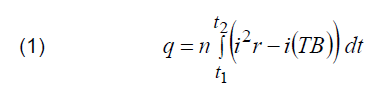
Provided that for battery heating during vehicle movement, the energy of 0.2-0.4 kWh would be spent, the vehicle would achieve range close to its maximum. During the construction of battery heating system, the process of cell self-heating was taken into account. The self-heating process stems from entropy change during electrochemical reactions [20,21] and from Joule heating due to current flow. The amount of heat generated in battery pack can be determined from the approximate equation (1).
.
where: q – indicator of generated heat (W); n – number of cells; i – current flowing through cells (A); r – cell internal resistance (Ω); T – temperature (K); B – temperature coefficient dependent on cell voltage drop and temperature rise caused by that drop (V/K).
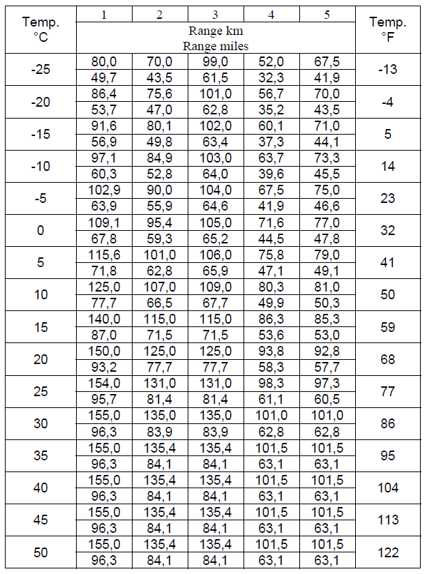
The testing period encompassed an entire year, which allowed acquiring data on vehicle and its battery performance in many different conditions and situations. The car under test was driven with various driving styles from 100% charged condition to the moment the onboard BMS system indicated, that the battery was completely discharged. The data was recorded using a recorder described in [22]. Every voyage recording was then analyzed and compiled into table 1 and figure 9.
The postulated MSEV solution seems to be justified, especially concerning the fact that without it, the vehicle operating in identical conditions would have its range limited by about 30-40%. Thanks to battery heating system the performance and efficiency of whole battery pack is increased.
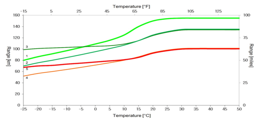
Table 1 and figure 9 show relationship of obtained vehicle range depending on battery pack temperature. The MSEV’s battery control capability was also tested. The plot shows operating conditions: operation without turning on of the vehicle’s auxiliary systems (curves 1 and 2) where curve 1 shows the maximal achieved range (best case) during testing at a particular temperature; curve 4 shows operation with cabin cooling/heating turned on; curve 3 shows operation with battery heating turned on; curve 5 shows operation with battery heating and cabin cooling/heating turned on. From the data on the plot it can be observed, that use of the battery heating system can increase vehicle range in comparison to identical conditions where heating system was inactive or not present.
The table 1 contains the basic parameters of the batteries used in electric vehicles.
Table 1. Vehicle range as a function of temperature
Numbers columns in the table correspond to the curve shown in figure 9.
The presented research shows that application of battery heating system in low ambient temperature can increase vehicle range by more than 30%. Bearing in mind the average vehicle range of 100-130km (60-80 miles), the loss of 30-40km (18-25 miles) can have considerable impact on during long voyages.
Another important issue from the point of view of electric vehicle operation is the positive impact of application of battery heating system resulting in significant increase in cycle count achieved during battery life.
Use of electric vehicle in low ambient temperature without the battery heater can cut the lifetime of the battery even by half [4]. In this case, the battery replacement implies significant costs which add up to the total operating cost of the electric vehicle. Speaking of EV operating cost, utilization of the MSEV can cut these even by half. This effect can be obtained by charging the vehicle only at a time when energy from the grid is cheaper.
For instance, in Poland, one kilowatt-hour (kWh) of electrical energy during the day costs about 20 USA cents, whereas during the night between 10PM and 6AM it’s worth only 10 cents. Therefore, it pays to use the MSEV thanks to which the user can wirelessly monitor the vehicle state using GSM/SMS technology.
During the road tests, at the beginning most users plugged in their vehicle in order to charge it almost immediately after returning home from work (at 4-5 PM). As a result, the battery was charged for at most 8 hours, and had finished charging till midnight. The charging took place during the time of higher electricity price for 6 hours, and only at most 2 hours during the lower price time period. It has to be stated, that during the road tests, very rarely was the battery discharged completely, so almost all the energy replaced in the battery was the energy with the higher price. Charging the battery during the time of lower electricity price by using the MSEV’s function of automatic two-way charger start in user controlled intervals could reduce the charging cost by about 60% (8 hours of charging during low electricity price period).
Fig.9. The plot of distance traveled by the vehicle depending on the temperature of the LiFePO4 battery pack and state (on or off) of vehicle auxiliary systems.
1 – maximum range (best case) achieved by vehicle with auxiliary systems turned off; 2 – average range achieved by vehicle with auxiliary systems turned off; 3 – average range, operation with battery heating turned on; 4 – average range, operation with cabin cooling/heating turned on; 5 – average range, operation with battery heating and cabin cooling/heating turned on
The advantage of MSEV is that the user can control and monitor the vehicle parameters (battery voltage, ambient, battery and cabin temperature; charging current and state; cabin heating, vehicle position and speed, etc.) using his GSM mobile phone. The user can also configure the MSEV in a way to automatically initiate the charging process or turn on the cabin heating so the travel can be made in the comfort of warm cabin right from the start. The MSEV can turn on battery heating automatically in case the ambient temperature drops below set value. Using data from sensors and GPS, the MSEV can inform the user remotely by the GSM network about vehicle location and state (voltages, currents, temperatures, etc.) Additionally, the MSEV can remotely alert the user about on board fire hazard.
Summary
This work wants to present an alternative mean of battery electric vehicle operation. It presents the results of tests of battery pack operating in low temperature environment. Thanks to the MSEV, a stress free operation of electric vehicle is possible, being it a car, an ATV, a motorbike, a scooter, a bicycle or a boat. The system functions permit vehicle use both in moderate and extreme temperature conditions, where -25°C (-15°F) ambient temperature is occurring. The use of GSM/GPS modules allows permanent monitoring of vehicle parameters as well as its remote control which can lead e.g. to charging cost reduction, by charging during hours when price of electric power is lower.
Using Artificial Intelligence methods residing inside the computer board, such as fuzzy logic or cognitive system it is possible to prevent damage to the battery which could potentially happen during use at low temperature environment and minimize the number of activities connected with the maintenance of the battery pack.
System can remotely check weather forecast and then request the user to plug the vehicle into the power socket to heat up the battery before driving.
According to the driver’s preference, the system allows to utilize the vehicle battery as an energy buffer for smart grid applications.
Application of the battery heating system increases comfort and passenger safety along with prolonging battery life which reduces total operation costs (approx. 60%) and increases time between battery replacements.
During the road tests (at low temperatures), a vehicle equipped with MSEV and battery heating system achieved 30% greater range than identical vehicle without such systems.
REFERENCES
[1] International Energy Agency. Global EV outlook 2016. Available: http://www.iea.org, (12.2016). [2] Pontes J., Europe Electric Car Sales. Available: http://evobsession.com/electric-car-sales, (12.2016). [3] Klippenstein M., Electric-Car Market Share In 2013: Understanding The Numbers Better. Available: http://www.greencarreports.com/news/1089555_electric-carmarket-share-in-2013-understanding-the-numbers-better, (12.2016). [4] Łebkowski A., Temperature, Overcharge and Short-Circuit Studies of Batteries Used in Electric Vehicles, Przegląd Elektrotechniczny, doi:10.15199/48.2017.05.13, (2017). [5] Senyshyn A., Mühlbauer M.J., Dolotko O., Ehrenberg H., Lowtemperature performance of Li-ion batteries: The behavior of lithiated graphite, Journal of Power Sources, Volume 282, (2015), p. 235–240. [6] Pesaran A., Santhanagopalan S., Kim G.H., Addressing the Impact of Temperature Extremes on Large Format Li-Ion Batteries for Vehicle Applications, 30th International Battery Seminar, Ft. Lauderdale, Florida, (2013). [7] Wu B., Ren Y., Li N., LiFePO4 Cathode Material – Chapter 11, Electric Vehicles – The Benefits and Barriers, ISBN 978-953-307-287-6, (2011). [8] Ouyang M., Chu Z., Lu L., Li J., Han X., Feng X., Liu G., Low temperature aging mechanism identification and lithium deposition in a large format lithium iron phosphate battery for different charge profiles, Journal of Power Sources, Volume 286, (2015), p.309–320. [9] Wang Y., Zhang C., Chen Z., A method for state-of-charge estimation of LiFePO4 batteries at dynamic currents and temperatures using particle filter, Journal of Power Sources, Volume 279, (2015), p.306–311. [10] Liu X., Wu J., Zhang C., Chen Z., A method for state of energy estimation of lithium-ion batteries at dynamic currents and temperatures, Journal of Power Sources, Volume 270, (2014), p.151–157. [11] Zou Y., Hu X., Ma H., Li S.E., Combined State of Charge and State of Health estimation over lithium-ion battery cell cycle lifespan for electric vehicles”, Journal of Power Sources, Volume 273, (2015), p.793–803. [12] Feng F., Lu R., Zhu C., A Combined State of Charge Estimation Method for Lithium-Ion Batteries Used in a Wide Ambient Temperature Range, Energies 2014, Volume 7, (2014), p.3004-3032. [13] Isizoh A.N., Okide S.O., Anazia A.E., Ogu C.D., Temperature Control System Using Fuzzy Logic Technique, International Journal of Advanced Research in Artificial Intelligence (IJARAI), Volume1, No.3, (2012). [14] Singhala P., Shah D.N., Patel B., Temperature Control using Fuzzy Logic, International Journal of Instrumentation and Control Systems (IJICS), Volume4, No.1, (2014). [15]Ramanathan P., Fuzzy Logic Controller for Temperature Regulation Process, Middle-East Journal of Scientific Research, Volume 20, (2014), p.1524–1528. [16] Łebkowski A., Exploitation tests of an electric powertrain with IGBT inverter for an EV Fiat Panda, Maszyny Elektryczne – Zeszyty Problemowe Nr 1/2016 (109), (2016), p.25-30. [17] Łebkowski A., Operational tests of an electric powertrain with MOSFET inverter for an EV Fiat Panda 2″, Maszyny Elektryczne – Zeszyty Problemowe Nr 1/2016 (109), (2016), p.71-75. [18] Zhang J., Ge H., Li Z., Ding Z., Internal heating of lithium-ion batteries using alternating current based on the heat generation model in frequency domain, Journal of Power Sources, Volume 273, (2015), p. 1030–1037. [19] Cai G., Guo R., Liu L., Yang Y., Zhang C., Wu C., Guo W., Jiang H., Enhanced low temperature electrochemical performances of LiFePO4/C by surface modification with Ti3SiC2”, Journal of Power Sources, Volume 288, (2015), p.136–144. [20] Chen Y., Evans J., Three – Dimensional Thermal Modelling of Lithium – Polymer Batteries under Galvanostatic Discharge and Dynamic Power Profile, Journal of Electrochemical Society, Volume 141, (1994), pp. 2947–2955. [21] Thomas K.E., Newman J., Heats of mixing and of entropy in porous insertion electrodes, Journal of Power Sources, Volume 119–121, (2003), p.844–849. [22] Łebkowski A., Electric Vehicle Data Recorder, Przegląd Elektrotechniczny, doi:10.15199/48.2017.02.62, (2017).
Author: dr inż. Andrzej Łebkowski, Akademia Morska w Gdyni, Katedra Automatyki Okrętowej, ul. Morska 83, 81-225 Gdynia, E-mail: andrzejl@am.gdynia.pl.
Source & Publisher Item Identifier: PRZEGLĄD ELEKTROTECHNICZNY, ISSN 0033-2097, R. 93 NR 9/2017. doi:10.15199/48.2017.09.09
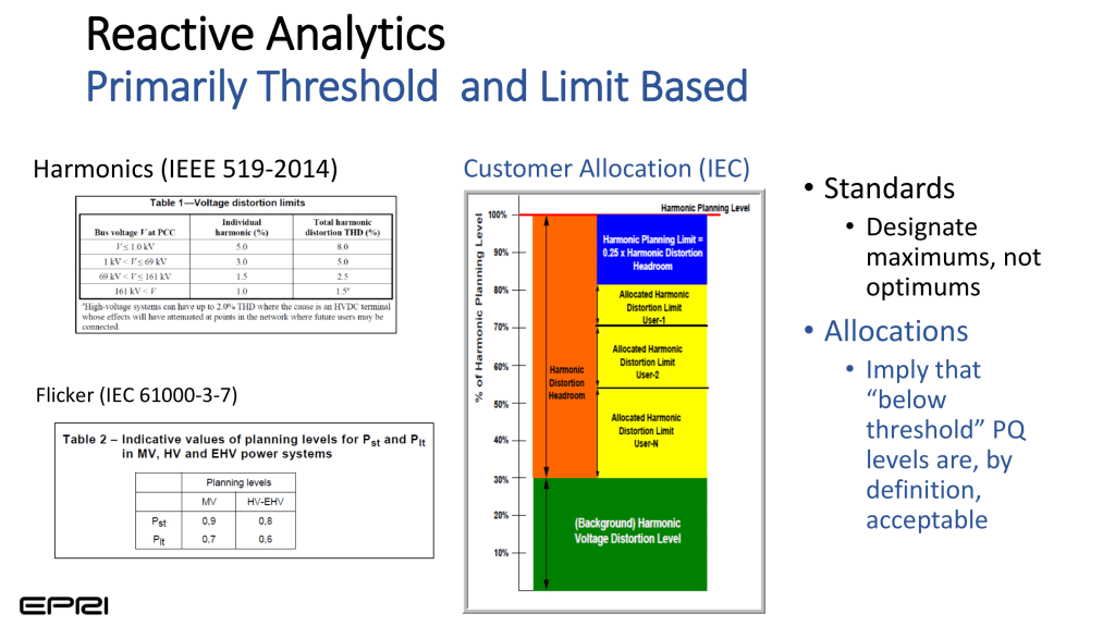
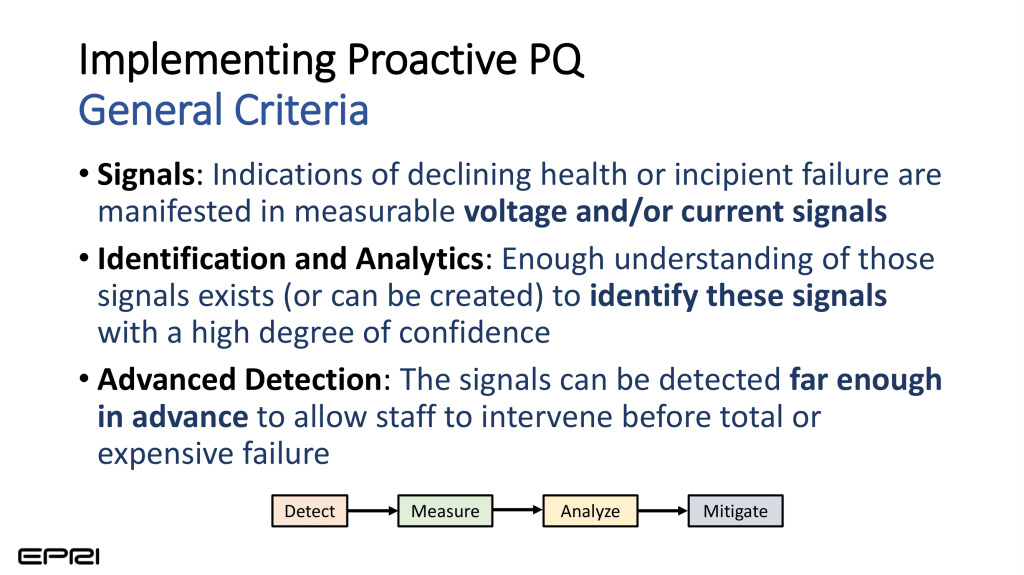
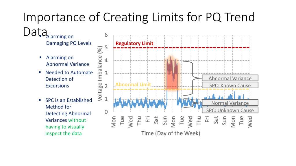
Published by Bill William Howe, Sr. Program Manager, Power Quality, Electric Power Research Institute (EPRI), USA. Email: BHowe@epri.com
Presented at 21st Annual PQSynergyTM International Conference & Exhibition, Sept 18th – 19th 2023. Mövenpick Hotel Sukhumvit 15 Bangkok, Thailand. Website: pqsynergy.com
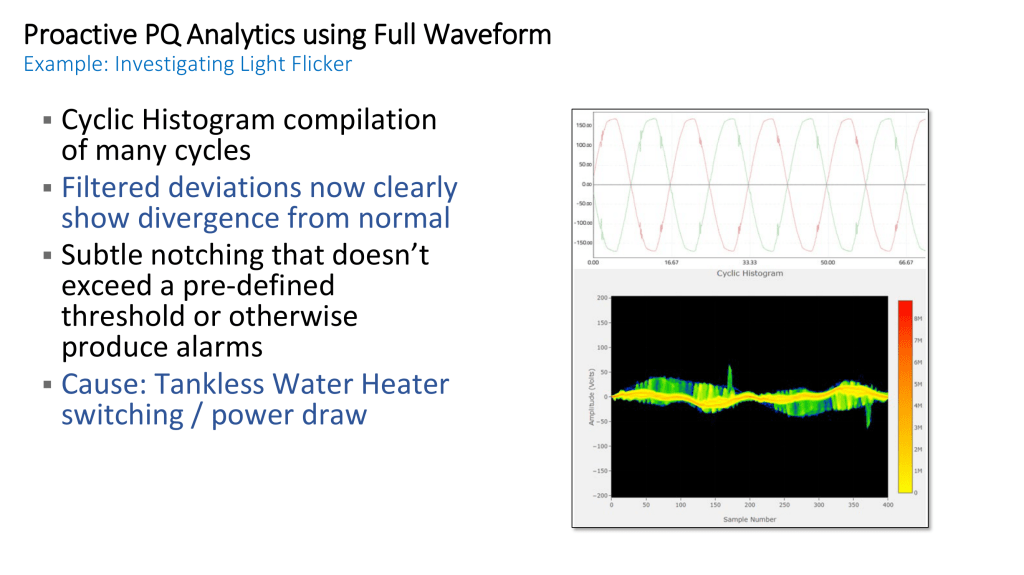
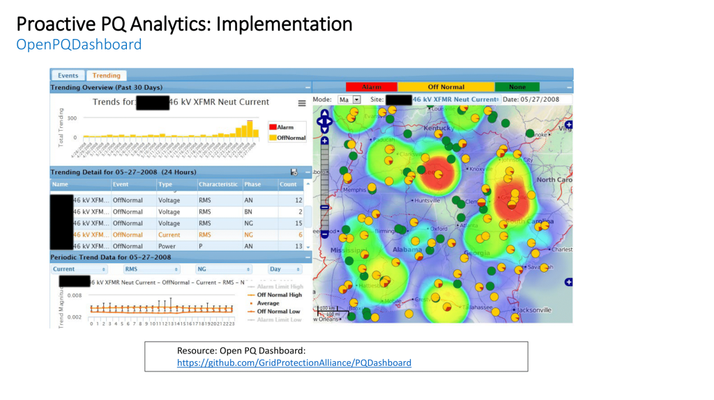
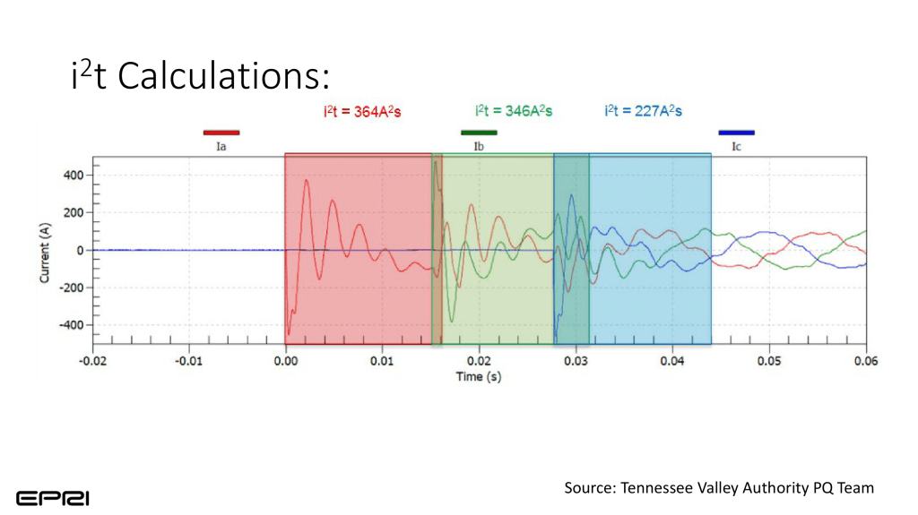
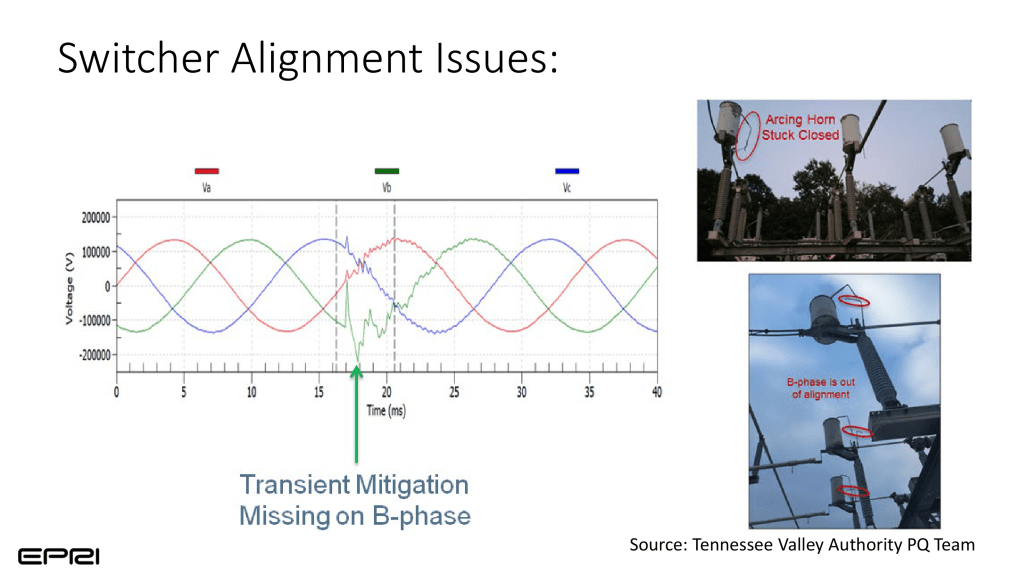
.
.
.
.
.
.
.
.
.
.
.
.
.
Bill Howe, Sr. Program Manager, Power Quality, EPRI.
Author: Bill Howe, Sr. Program Manager, Power Quality, Electric Power Research Institute (EPRI), USA. Email: BHowe@epri.com
Bill Howe is the Program Manager for Power Quality Research (Program 1) in the Power Delivery and Utilization Sector. Mr. Howe’s primary areas of expertise are: power quality research, information and knowledge development and deployment, industrial and commercial power quality analysis, industrial and commercial electric and control system design and optimization, demand response, electric energy efficiency, and market research.
Mr. Howe manages the PQ Research portfolio for EPRI. His key responsibilities are strategic planning, project management, information products, and multi-client studies covering topics related to quality, reliability, and efficiency of energy delivery.
Before joining EPRI, Mr. Howe worked nearly 20 years in management and senior engineering positions within a number of Fortune 500 companies, and has experience in medium-voltage power quality product development, product testing, substation and distribution-system design and construction, motors and drive systems, and process automation. He is a registered professional engineer.
Published by Kevin Clemens, EE Power – Technical Articles: An Introduction To Flow Batteries, February 06, 2023.
Lithium-ion batteries get all the headlines, but flow batteries are a viable option, particularly for large-scale grid storage.
Lithium-ion batteries have become the energy storage device of choice for cell phones, laptop computers, personal handheld devices, and electric vehicles (EVs). The high energy density of a lithium-ion cell helps it store large amounts of energy without too much weight or taking up too much space. Lithium-ion batteries are also finding use in stationary storage applications such as renewable energy grid storage and backup power supplies for computer systems and critical medical equipment.
Image 1: Diagram of a flow battery. Image used courtesy of Colintheone, CC BY-SA 4.0, via Wikimedia Commons
Although the price of lithium-ion batteries has come down in recent years, thanks largely to the demand of the EV industry, the technology is still relatively expensive. It has other issues like a limited lifetime and the potential to cause fires if they are over- or under-charged. Traditional lead acid batteries can also be used in these applications but do not have the energy density, charging rate, or capacity that a lithium-ion battery can provide.
Flow Batteries
Lithium-ion batteries are one of many options, particularly for stationary storage systems. Flow batteries store energy in liquid electrolyte (an anolyte and a catholyte) solutions, which are pumped through a cell to produce electricity. Flow batteries have several advantages over conventional batteries, including storing large amounts of energy, fast charging and discharging times, and long cycle life.
The most common types of flow batteries include vanadium redox batteries (VRB), zinc-bromine batteries (ZNBR), and proton exchange membrane (PEM) batteries.
Vanadium Redox
Vanadium redox batteries are the most widely used type of flow battery. They use two different solutions of vanadium ions, one in a positive state (V(+4)) and one in a negative state (V(+5)), which are separated by a membrane. Charging causes the vanadium ions to be oxidized and reduced, causing the electrical potential to increase. When the battery is discharged, the vanadium ions flow through the membrane, generating an electrical current.
Several companies are supplying VRB systems around the world. Invinity Energy Systems has more than 45 megawatt-hours (MWh) of vanadium flow batteries deployed or contracted at sites worldwide. Invinity’s largest installation is a 2 megawatt (MW)/8MWh flow battery co-located with a 6 MW solar photovoltaic (PV) array on land adjacent to Yadlamalka Station, a 1,000 square kilometer sheep and cattle farm in Australia.
Image 2: Invinity flow batteries are sited at Yadlamalka station in Australia. Image used courtesy of Invinity Energy Systems
Zinc-Bromide
Zinc-bromine (ZNBR) batteries are the oldest type of flow battery (1879) and use zinc and bromine ions to store electrical energy. Their high energy density makes them ideal for large-scale energy storage systems. Zinc-bromine batteries have been used for several decades in various applications, including utility-scale energy storage and backup power systems.
A solution (electrolyte) of zinc-bromine is stored in two tanks. The solution is pumped through a reactor stack comprising two compartments separated by a micro-porous membrane made from polyolefin.
The electrolyte on the negative (anode) side is water-based, while the electrolyte on the positive side contains an organic amine compound. This amine is used to hold the bromine in the solution. When the ZNBR battery is charged, zinc metal is plated as a film on the anode side of a plastic-composite electrode. At the same time, bromide ions oxidize into bromine and form a byproduct that sinks to the bottom of the cathode electrolyte tank. When the battery is discharged, the plated zinc metal is oxidized and dissolved in the aqueous electrolyte, releasing two electrons to the anode used to power an electric device. As the electrons return through the cathode (positive electrode), the bromine in the amine byproduct is converted into two negative bromide ions and combined to form a zinc bromide solution.
Unlike a lithium-ion battery with a 90 percent overall charge-discharge efficiency, a ZNBR is in the 65-75 percent efficiency range. Redflow in Australia and Primus Power in the U.S. are two companies commercializing zinc-bromine flow batteries. A ZNBR battery is scalable through the size of the electrolyte tanks: Redflow makes a 10 kilowatt-hour (kWh) system, while Primus Power has a 125 kWh unit.
Image 3: ZBM3 zinc bromide flow battery. Image used courtesy of Redflow
Proton Exchange Membrane
Proton exchange membrane (PEM) flow batteries use a proton-conducting membrane to separate the positive (cathode) and negative (anode) electrodes. PEMs are a newer type of flow battery and act as a combination of electrolyzer, using charging electrical energy to split water into hydrogen and oxygen, and a fuel cell, combining the hydrogen and oxygen like a fuel cell during discharge to produce free electrons. A solid-state metal hydride electrode can be used as one of the electrodes to store the hydrogen that forms during charging.
Because of their higher power density, PEM flow batteries are being discussed for use in EVs to replace lithium-ion batteries. Like lithium-ion cells, they exhibit high efficiency, losing little energy between the charge and discharge cycles.
Image 4: PEM flow battery. Image used courtesy of RMIT University
What’s Next for Flow Batteries?
In the future, flow batteries will play a crucial role in developing renewable energy systems. Renewables like solar and wind energy need energy storage to store excess energy generated during periods of high production and release it during periods of low production.
Flow batteries are ideal for this problem, as they can store large amounts of energy and release it quickly when needed. Flow batteries are also expected to be used in microgrid systems, which are small-scale energy grids independent of the traditional electrical grid. Microgrids are becoming increasingly popular as they provide a more reliable power source, especially in rural areas or areas prone to power outages. Additionally, flow batteries are useful in backup power systems to provide electrical support during power outages and natural disasters.
As the number of EVs on the roads has increased dramatically, the demand for lithium in their batteries will continue to grow. Flow batteries provide a viable alternative to using lithium-ion batteries in grid storage, saving lithium for EVs.
Author: Kevin Clemens has spent more than 30 years writing about transportation, energy, technology, and sustainability.
Published by Maytham S. AHMED1,2 Azah MOHAMED1 , Raad Z. HOMOD3 , and Hussain SHAREEF4, Dept. of Electrical, Electronic & System Engineering, Faculty of Engineering & Built Environment, Universiti Kebangsaan Malaysia (1) General Directorate of Electrical Energy Production- Basrah, Ministry of electricity, Iraq (2) Dept. of Oil and Gas Engineering, Basrah University for Oil and Gas, 61004 Basrah, Iraq (3) Dept. of Electrical Engineering, United Arab Emirates University, P.O. Box 155511 Al-Ain, UAE (4)
Abstract. In the last decades, home energy consumption has increased significantly due to increasing load demand in the residential sector. This paper presents a home energy management (HEM) algorithm to manage the home appliances in a house during a demand response (DR) event. The developed algorithm considers load appliances according to customer preference setting, priority of appliance, and comfortable lifestyle that can be changed at any given time and performs DR at appliance level. The load models are developed based on the operational and physical characteristics for the purpose of DR strategies. Appropriate residential load models are required to support the DR strategies and therefore air conditioner, water heater, electric vehicle and washing machine are chosen as the loads. The proposed HEM algorithm is shown to be effective in managing power consumption at appliances level and can maintain the total household power consumption below its demand limit (DL) without affecting the comfort level.
Streszczenie. W artykule predstawiono algorytm do zarządzania konsumpcja energii w gospodarstwach domowych. Algorytm zarządza enegią przy założonym poziomie dopuszczalnego limitu I bazuje na charakterystykach urządzeń podłączonych do sieci. Algorytm zarządzania konsumpcj a enegii w gospodarstwach domowych
Keywords: Home energy management, demand response, smart appliance, energy efficiency, peak load reduction. Słowa kluczowe: konsumpcja energii, gospodarstwo domowe, algorytm HEM
Introduction
Electricity power consumption varies between seasons of the year, and days of the week, where the highest peak hour demands typically happens when the weather temperature is high. In several situations, especially in the summer season, end user has to pay more than the normal electricity price because of increased energy consumption for cooling purposes [1]. Residential load represents the largest energy consumption and to reduce the electricity generation cost, DR is practiced by utility by decreasing the peak demand and shifting the home appliances from peak hour demand to off-peak hours [2]. Thus, shifting and scheduling electricity usage to off peak hours is essential to both end users and utility companies for reducing cost of electricity [3].
DR refers to a program which offers incentives to homeowners who curtail their energy use during times of peak demand. DR applications are designed to reduce peak demand and encourage end-users to reduce energy consumption.
In recent years, residential HEM with DR has become an active topic for many research studies [4]. Previous research highlighted that the use of DR is essential to improve HEM system in the domestic sector [5]. For efficient HEM system with DR, a variety of consumer electronic devices must be controlled using the internet and the home network for remote management so as to reduce peak demand that may lead to reduce risk of outages at distribution and transmission networks [6]. Load models need to be developed to evaluate DR at the distribution circuit level so as to study customer behaviours. Recently, various optimization techniques have been used to assist homeowners to create optimal appliance scheduling and shifting of energy usage based on variety pricing scheme programs, feed-in tariffs, and comfort settings [7]. In [8], the immune clonal selection algorithm has been developed for HEM to reduce the power consumption of air conditioner and water heater. A framework of HEM system using artificial bee colony optimization algorithm has been developed to improve the system by scheduling the home appliances [9]. An optimal HEM approach based on the game theory is used to reduce the peak-average electricity consumption rate [10]. The rule based technique has been applied to reduce electricity bill considering residential DR application [11]. In [12], the operation of the home appliances schedule is according to the ever-changing real time prices and the tariff rate based DR program. A smart plug with a wireless Zigbee sensor developed for measuring power consumption of electrical appliances in the HEMS [13].
One of the major challenges in scheduling household appliances is to minimize the energy consumption without affecting the customer’s comfort. However, most of previous research works have focused on saving energy to reduce electricity bill without considering residential comfortable lifestyle.
In this paper, a HEM algorithm has been developed by considering customer’s comfort for household peak load reduction to reflect any desired DR event. The DR enabled load model at the appliance level is used to achieve energy savings and reduce electricity bill based on shifting the operation of several appliances to specific off peak time. In this study, four home appliance models have been considered according to the customer preferences and priority of appliances that include air conditioner (AC), water heater (WH), electric vehicle (EV), and washing machine (WM). Hence, the proposed HEM algorithm is developed to reduce power consumption at peak time and shifting the appliances to off peak time without affecting the customer’s comfort.
Demand response enabled home load appliances
To develop a HEM algorithm for residential customers with DR applications, there is need to know the characteristics of home appliances and preferences of the loads. In this research, only controllable loads such as AC, WH, EV, and WM are deemed to be controlled according to priority of appliances, comfort level and customer preferences, so as to participate in the HEM system. The physical model of the loads is used as an appliance that is considered in the developed HEM algorithm. Figure 1 shows the HEM architecture with AC, WH, EV, and WM as appliances connected to the controller.
Fig.1. HEM architecture
In Figure 1, the DR signal with information on the duration, situation and amount of load to be shed is received directly from a smart meter in the HEM system [14]. Thereafter, the HEM algorithm controls the off/on states of the appliances according to the demand limit, appliance priority, DR request and comfort level set by the consumer. The characteristics and preferences of the loads are shown in Table 1.
Table 1. Load priority and characteristics
.
Table 1 show that the first priority is AC and that the room temperature should be maintained in the range of 23.33–25.56°C. The second priority is WH with the hot water temperature maintained within the acceptable range of 43.33–48.8°C. EV is the third priority in which EV is assumed to have a fully battery charged by 8:00 morning at the next day. For WM, a consumer can identify its completion time and maximum on time of heating coils as 90 minutes. Other non-controllable loads are assumed to exist but are not considered in the system. The following subsection describes the load characteristics of AC, WH, EV and WM.
Air conditioner
An AC extracts unwanted heat from an area. When a demand limit is enforced and the AC is turned on, while the room temperature maintains within a comfortable range, the controller will impose the AC to turn off. If the temperature of room reaches its maximum allowable temperature, the AC unit will turn on, and the room temperature will be regularly reduced. At the time the room temperature decreases to its allowable set point temperature of, the main switch will turn off the AC and the temperature of room will maintain within the comfort level. In the case when the room temperature is between 23.33 and 25.56°C, the controller will keep the AC at the status of devices as shown in Eq. (1)
.
where mhvac is the status of device, mhvac,=1 device is switched on, and if mhvac,,= 0 device is switched off, Thvac,t is the temperature of room in °C at time interval t. The AC power consumption (Phvac,t) can be calculated by using:
.
Electric water heater
A domestic WH consists of a thermostat to sense temperature and switch ON / OFF to heat the water [15]. When the water temperature reaches its minimum allowable temperature of set point, 43.33°C, the WH will switch on to maintain the temperature of water at its comfortable range. If the temperature reaches its maximum allowable temperature of set point,48.89 °C, then the WH will switch off the heater. When the water temperature is within 43.33– 48.89 °C, the heater switch status will keep the previous device state. In the simulation, the second highest priority is WH and it is the second to the last device to be switched off.
The status device of water heater (mwh) at a given interval time is given as follows
.
Where mwh is the status of device, mwh=0 means the device is switched off, mwh=1 indicates that the device is switched on and Twh,t is the temperature of hot water in °C at interval time t.
The WH power consumption in kW (Pwht) at a given time interval can be determined using,
.
where Pwh is the amount of WH power rated in kW.
Electric vehicle
Battery is used to power up the motor of EVs. To model an EV, there are three parameters that should be taken into account; the rated charging power, plug-in time and state of charge (SOC) battery. The SOC of an EV battery is assumed to vary between 20% and 100% [16]. The time it takes to fully charge an EV depends on rated charging power, plug-in time and the battery SOC. In this research, EV is assumed to be plugged in when its battery SOC reaches 20% and the EV will not be used until the battery is fully charged. The switch status of EV (mev) at time intervals can be calculated using,
.
where mev is the device status, mev= 0 means that the appliance is switched off, mev=1 means the appliance is switched on, and SOCev,t is the battery SOC in the time interval.
The EV power consumption in kW, Pevt at a given time interval can be determined by
.
where Pev is the amount of rated EV power in kW.
Washing machine
The electrical power consumption of a WM are rotating tumbler motor and heating coils. The load model of a WM and rated power for each time interval is adopted from [18]. A WH will switch on and need at least a 90-minute interval time so as to complete its job. The WH will switch off the motor, when the total on time arrived to the wanted time. The switching status of WM (mwm) can be determined as follows:
.
where mwm is the device status, mwm=0 means the appliance is switched off, mwm=1 means the appliance is switched on, and twm,t is the time interval for WM in minutes.
The WM power consumption in kW, Pwmt at a given interval time can be determined by
.
where Pwm is the amount of WM power rated in kW
Fig.2. Flowchart of the HEM algorithm considering load priority
Proposed HEM algorithm
The proposed algorithm is developed such that it can control AC, WH, EV, and WM and switch customer load so as to decrease the cost of electrical power consumption. The HEM algorithm starts by reading the data and information of all the above mentioned appliances. Each appliance is compared with several set points including load priority, power consumption and customer preference settings on the temperature of AC and WH. If the total electrical power consumption (PT) is greater than the demand limit (DL), the algorithm will turn OFF the lower appliance priority starting with WM, and force the loads to shift their operating time after ending the period of DR event in order to keep the total power consumption below its DL. In addition, the HEM algorithm issues a control signal to turn ON the appliance when the total household load is below its DL level. In this way, the HEM will optimize the scheduling of the appliances while maintaining the PT below its DL. The HEM algorithm is illustrated in terms of a flowchart as shown in Figure 2.
The proposed HEM algorithm implementation steps are described as follows:
i. From Table 1, read the characteristic of all appliances such as its rated power.
ii. Specify the user input data such as load priority, hot water temperature, room temperature, comfort level, real time pricing (RTP), and user demand limit (UDL).
iii. Read utility data signal of DR, demand limit in kW and the value of load shed (LS).
iv. The new demand limit (NDL) is determined by using equationNDL = UDL – LS.
v. Specify the device status for all appliances by using equations (6), (7), (9) and (11) and using the household electrical energy consumption equations (4), (8), (10) and (12) to determine the current demand (D).
vi. Update the appliances status such as the priority number of devices in service.
vii. Apply the condition in which if NDL is greater than D, then go to step ii.
viii. If the NDL is lower than D, then the appliance will switch OFF according to the level of comfort and priority of appliance and go to step v.
Simulation results
The simulation results and the performance of the proposed HEM algorithm in managing the consumption of electrical appliances as described accordingly. Two case studies were considered to describe the implementation of the algorithm. The first case is without applying DL so as to clarify the performances of AC, WH, EV, and WM as shown in Figure 3. The parameters and model specifications, such as the dimensions of WM and car characteristics, are taken from [17, 18].
Fig.3. Pattern of electrical energy consumption without DL (a) AC, (b) WH, (c) EV, (d) WM, (e) PT
The AC unit maintains the temperature of room at a comfortable range by turning OFF/ON as shown in Figure 3(a). More time is needed to cool a room at noon and hence, more power is consumed. The variation of WH temperatures with ON/OFF characteristics is shown in Figure 3(b). The WH operates to bring the temperature of water to the range of comfort level set at 43.33– 48.89°C. Similarly, at midnight the EV starts charging with 20% state of charge, as depicted in Figure 3(c). The EV is fully charged in five hours and forty-eight minutes. In Figure 3(d), the WM operates twice at 12:00 p.m and 6:00 p.m consuming 4 kW. Each time, the WM needs at least one and a half hours to complete its job. Finally, the total the household power consumption, PT is shown in Figure 3(e). The figure indicates that the maximum demand cannot be controlled and it depends on the device usage time.
In the second case, assumed the DR event is imposed by the power utility with 2 kW DL between 17 to 22 hours, as shown in Figure 4.
Fig. 4. Pattern of electrical energy consumption with DL of 2kW (a) AC, (b) WH, (c) EV, (d) WM, (e) PT
With DL, the WM, WH and EV have to be switched OFF and only one appliance which is the AC can be operated and draws 1.25 kW. The WM and WH require their schedules to be shifted after the period of DL. The results explain the ability of the proposed HEM algorithm in preserving total electrical energy consumption below the DL value. The algorithm prevents exceeding the total power consumption of the selected DL value.
Conclusion
A HEM algorithm with DR has been developed to schedule the operation of home appliances to save energy costs by considering customer convenience as well as characteristics of electric appliances. Accurate load models considering AC, WH, EV and WM have also been developed according to its operational and physical characteristics. The HEM algorithm has been implemented by considering the operation of loads such as AC, WH, EV and WM with DR signal to alleviate high energy consumption in the home. The results of the HEM algorithm showed that it is capable of preserving the total electrical energy consumption below the selected DL value and managing household loads taking into consideration customer’s preference settings and load priority. The algorithm can easily be implemented in homes because of its flexibility in controlling different types of home appliances.
Acknowledgment: The authors gratefully acknowledge University Kebangsaan Malaysia for the financial support on the project under the research grant DIP-2014-028
REFERENCES
[1] Zhang X., Shahidehpour M., Alabdulwahab A., Abusorrah A., Hourly Electricity Demand Response in the Stochastic Day-Ahead Scheduling of Coordinated Electricity and Natural Gas Networks, IEEE Trans on Power Syst. 31 (2016) 592-601. [2] Maharjan S., Zhu Q., Zhang Y., Gjessing S., Basar T., Demand Response Management in the Smart Grid in a Large Population Regime, IEEE Trans on SG. 7 (2016) 189-199. [3] Moreno-Munoz A., Bellido-Outeirino F.J., Siano P., Gomez-Nieto M.A., Mobile social media for smart grids customer engagement: Emerging trends and challenges, Renewable and Sustainable Energy Reviews. 53 ( 2016)1611-1616. [4] Ahmed M.S., Mohamed A., Homod R. Z., Shareef H., Real time optimal schedule controller for home energy management system using new binary backtracking search algorithm, Energy and Buildings. 138 (2017) 215-227. [5] Kushiro N., A Basic Study for Realizing Life Event Sensor for Home Energy Management System, Knowledge-Based information systems in Practice. Springer International Publishing, (2015) 21-38. [6] Patel K., Khosla A., Home energy management systems in future Smart Grid networks: A systematic review, IEEE NGCT. (2015) 479-483. [7] Gudi N., Wang L., Devabhaktuni V., A demand side management based simulation platform incorporating heuristic optimization for management of household appliances, Int. J. Electr. Power Energy Syst. 43 (2012) 185–193. [8] Hong Y. Y., Chen C. R., Yang H W., Implementation of demand response in home energy management system using immune clonal selection algorithm, IEEE CEC conf. (2015) 3377-3382. [9] Zhang Y., Zeng P., Zang C., Optimization algorithm for home energy management system based on artificial bee colony in smart grid, IEEE CYBER conf. (2015) 734-740. [10] Mohsenian-Rad A H., Leon-Garcia A., Optimal residential load control with price prediction in real-time electricity pricing environments, IEEE Trans on SG. 2 (2010)120-133. [11] Ahmed M. S., Shareef H., Mohamed A., Ali J. A., Mutlag AH. Rule Base Home Energy Management System Considering Residential Demand Response Application, Appl Mechanics & Materials. 785 (2015) 526-531. [12] Li X. H., Hong S. H., User-expected price-based demand response algorithm for a home-to-grid system, Energy. 64(2014) 437-49. [13] Ahmed M.S., Mohamed A., Homod R. Z., Shareef H., Sabry A. H., Khalid K.B., Smart plug prototype for monitoring electrical appliances in Home Energy Management System, IEEE SCOReD conf. (2015) 32-36. [14] Wehierek P., Konarski M., Electricity measurement accuracy in the smart metering system, Electrical review, R. 91 NR 3 / 2015. [15] Ahmed M.S., Mohamed A., Homod R. Z., Shareef H., Khalid K., Modeling of Electric Water Heater and Air Conditioner for Residential Demand Response Strategy. International Journal of Applied Engineering Research. 11 (2016) 9037-9046. [16] Fiori C., Ahn K., Rakha H. A., Power-based electric vehicle energy consumption model: Model development and validation, Applied Energy. 168 (2016) 257-268. [17] Chi S., Zhang Z., Xu L., Sliding-mode sensorless control of direct-drive PM synchronous motors for washing machine applications, IEEE Trans on IA. 45 (2009) 582-90. [18] Ahmed M.S., Mohamed A., Homod R. Z., Shareef H., Hybrid LSA-ANN Based Home Energy Management Scheduling Controller for Residential Demand Response Strategy, energies. 9 (2016) 716.
Authors: Maytham S. Ahmed is a PhD student in the Department of Electrical, Electronic and Systems Engineering, Universiti Kebangsaan Malaysia (UKM), E-mail: eng_maitham@yahoo.com. Azah Mohamed is a professor in the Department of Electrical, Electronic and Systems Engineering, Universiti Kebangsaan Malaysia (UKM), E-mail: azah@eng.ukm.my. Raad Z. Homod is a professor in the Dept. of Petroleum and Gas Engineering, Basrah University, Iraq, E-mail: raadahmood@yahoo.com. Hussain Shreef is a professor in the Department of Electrical Engineering, United Arab Emirates University E-mail: hussain_ln@yahoo.com.
Source & Publisher Item Identifier: PRZEGLĄD ELEKTROTECHNICZNY, ISSN 0033-2097, R. 93 NR 3/2017, doi:10.15199/48.2017.03.46.
Published by Paweł PIJARSKI, Sylwester ADAMEK, Robert JĘDRYCHOWSKI, Klara SEREJA, Lublin University of Technology, Department of Electrical Networks and Security
Abstract. An increasing number of connected prosumer installations, mainly photovoltaic ones, can cause problems with the operation of lowvoltage networks such as voltage fluctuations. These problems can be solved by an adequate control of the sources operation within one transformer substation. The article presents a concept of a controller that ensures access to the data that describe the network operating conditions and the energy sources installed there as well as allows control of the micro installations output power.
Streszczenie. Coraz większa liczba przyłączanych instalacji prosumenckich, głównie fotowoltaicznych, może być przyczyną występowania problemów w pracy sieci niskiego napięcia, takich jak m.in. wahania napięcia. Problemy te mogą być rozwiązane poprzez odpowiednie sterowanie pracą źródeł w obrębie jednej stacji transformatorowej. W artykule zaprezentowano koncepcję sterownika, który zapewnia dostęp do danych obrazujących warunki pracy sieci i zainstalowanych w niej źródeł energii, jak również umożliwia sterowanie mocą wyjściową mikroinstalacji. (Monitorowanie wpływu prosumenckich mikroinstalacji na parametry elektryczne systemów sieci niskiego napięcia).
Keywords: microgeneration, power quality, SCADA, Smart Grid. Słowa kluczowe: mikrogeneracja, jakość energii, SCADA, Smart Grid.
Introduction
The development of distributed generation will lead to the emergence in the low-voltage network of phenomena occurring so far in higher voltage networks. Particularly important will be phenomena causing changes in power flows and deterioration of power quality parameters, which pose potential threats for devices connected to the network. In order to counteract them, it will be necessary to monitor the work of those parts of the network in which a large number of micro-sources with a relatively high power have been installed. Analysis of the LV (low-voltage) network operation requires in such a case the implementation of complicated, multi-variant simulations and analyses, e.g. voltage conditions in the LV network with various levels of saturation with micro installations, different structure and load profile.
The essence of the problem
According to the relevant act [1], micro-installation is “a renewable energy installation with a total installed electrical power not exceeding 40 kW, connected to a power grid with a rated voltage lower than 110 kV or with a heat-generating power in the combination no greater than 120 kW”. The connection of low-voltage power sources of this type to end users, according to another act [2], can take place in two ways:
• on the basis of the notification, • by submitting an application for determining the terms of connection to the distribution network
The article focuses on the first of the above-mentioned ways of connecting micro-installations – based on the application.
The development of micro-installations, especially photovoltaics, caused by a drop in their prices seems to be unavoidable. As a consequence, one should expect various technical problems, among which the most serious will probably be voltage impact [3, 4], resulting from the power flow from the point of connection of these sources towards the MV/LV (medium voltage/low-voltage) substations. It results from the fact that the correlation of power generated in them with the demanded power is small.
Figure 1 shows that there are periods when the maximum power generated in a solar installation does not coincide with the maximum demand. This situation is unfavourable because it will cause power flows towards the MV/LV transformer and, as a result, contribute to the “voltage boosting” effect, which is the inverse of the voltage drop effect.
Fig. 1. Demand of a sample prosumer during a day in July and power generation in a solar installation
The solution to this problem can be:
• control of the reactive power of sources, • control of the active power of sources, • turning off the “necessary number of sources”.
Each of these methods has its advantages and disadvantages.
Proposal of control algorithm
Currently, no voltage regulation is carried out in low voltage networks in a continuous mode. In connection with the anticipated technical problems during the operation of sources, a grid control algorithm should be developed, taking into account the use of certain regulatory sources, or even, if necessary, limiting their power. An attempt to develop an analogous algorithm for medium voltage networks is shown, for example, in [4]. Voltage control in the low-voltage network will be possible after fulfilling several conditions:
• the network will be observable to a certain extent – voltage in selected nodes and powers generated in sources are known,
• we have information about the topology and parameters of network branches,
• we have an algorithm allowing to determine the value of extortion in the network (voltages, generated power), so as to ensure correct operation of the system,
• it is possible to send calculation results to generation devices in the network and change the parameters of their operation in accordance with current conditions.
The condition of observability of network operation parameters with the current state of technical solutions seems to be feasible. The network topology and its data are also possible to collect, although this process can be tedious due to the significant number of low-voltage lines.
Assuming that approximate voltage values can be determined, e.g. by using models analogical to those described in [4], the grid control algorithm should first of all eliminate any overruns, i.e. meet the condition:
.
where VN is the nominal voltage of the network, and Vi is the supply voltage at the i-th receiver.
Then, if the installed sources allow for adjusting their passive and active power, it is possible to optimise the system’s operation in such a way that the voltage deviations of the supplying power from the rated voltage are as low as possible. In practice, this would mean minimising the voltage quality indicator described in [4] and given by the formula:
.
where VN is the nominal voltage of the network, Vi is the supply voltage at the i-th consumer and n is the number of energy users. The practical implementation of the control algorithm will require the expansion of the network infrastructure with measurement and data transmission systems.
Control system
When organising a control system for the LV network with micro-sources connected, it is necessary to define the goals it should implement. They were indirectly defined in previous chapters and include:
• monitoring of electrical parameters at selected points of the LV network, cooperation with micro energy sources, • implementation of algorithms allowing for network operation control, • ensuring communication between cooperating elements of the system. • retransmission of data to the SCADA (Supervisor Control and Data Acquisition) system of the distribution network operator.
To realise these assumptions, the concept of a control system was developed, based on cooperating devices, creating a distributed architecture and working in a master-slave system.
The main element of the system is the master controller installed in the LV transformer substation MV/LV. It has several important functions, which include:
1. Measurement of basic electrical parameters on the LV transformer side and in outgoing circuits.
2. Determination of the criterial values necessary to assess the operation status of the network in the main circuit and individual outflows, allowing their assessment in the control process.
3. Implementation of the network control algorithms adopted for a given system described in the previous chapter.
4. Ensuring communication with individual slave controllers, taking into account the adopted communication technology.
5. Network monitoring, generation of warnings and alarms.
6. Controlling the operation of individual slave controllers, and thus the operation of energy sources, taking into account the specificity of individual sources.
7. Providing information to the network operator’s SCADA system. This will be information about measurement parameters and selected alarm signals.
8. Visualisation of the network and system operation status.
Nevertheless, slave controllers are also important. They are installed in the switchgears of the building or the LV installation connector to which the source has been connected. They perform functions of the source operation monitor, the power grid at the connection point and prosumer installation. Their tasks include:
1. Measurement of basic electrical parameters with special consideration of those that are necessary for the operation of the control algorithm. 2. Retransmission of data to the master controller. 3. Direct or indirect control of the operation of the source converter circuit, including the operation of the prosumer installation.
Low-power sources are connected to the network via inverters equipped with their own controllers. The operation of the slave controller can be analysed depending on the possibility of cooperation between the slave controller and the source controller.
In the least favourable case, when such cooperation for technical or other reasons is not be possible, the role of the controller will be limited to the measurement of the set values, their retransmission to the master controller. It would also be possible to disconnect the source in a prosumer installation in critical situations. In the second case, it is possible to assume supervision of the source operation through the local controller assigned to the inverter controlling its operation. The third case assumes full control over the source converter, which would allow the implementation of generation control algorithms directly in the slave controller. In all cases, it is necessary to maintain the autonomy of operation of local systems, so that even in the absence of communication with the master controller, safe operation of the source is guaranteed.
The presented control system can be implemented on the basis of existing solutions. The PLC controller is an example of this. Thanks to their modular structure, the controllers allow for extending the possibilities offered by classic automation devices [5].
Fig. 2. WAGO-I/O-SYSTEM 750 series PLC controller installed in the building switchboard
PLC controllers have a number of possibilities to obtain information about the operation of the LV network and prosumer installation through the controller modules and elements cooperating with them. The first group of elements includes measuring modules [6]. The second group of elements are communication modules allowing for exchange of information between controllers and other elements, e.g. source controller or energy meters. Communication is possible by using: links RS 232, RS 485, TCP/IP networks, wireless links.
Practical implementation of a LV network monitoring system
The practical implementation of the distributed monitoring system was carried out on cooperating controllers of the WAGO series 750-880/025 (Fig. 2) equipped with additional tele-control functions and a 15 kW photovoltaic system with a three-phase SMA inverter. For research purposes, resistors and reactors with adjustable setpoints allowing simulation of the LV line parameters were also used (Fig. 3).
Fig. 3. Scheme of the testing system
In the proposed solution, in order to conduct research experiments, the controllers work as master and slave and perform the partial tasks described in the previous section. The controllers implement both data acquisition functions and control functions. The slave controller has been equipped with an analogue input card for measuring voltages and currents in a three-phase system and binary outputs for controlling the inverter’s power limitations, using the intermediate relay separating the controller and the inverter. In addition, the controller has communication interfaces to view its work status, current measured values, remote programming as well as communication with the master controller. It should be emphasised that the power measurement carried out in the controller is informative, and the regulated parameter is voltage. The master controller also has a three-phase measurement module, binary inputs and outputs. However, its main task is the acquisition of data, including those obtained from the slave controller and the implementation of control algorithms for the network. The software part of the project was created in the CoDeSys environment used for programming PLC applications.
The measuring modules used in both controllers to monitor selected electrical circuits allow for three-phase measurement of selected electrical parameters. The current measurement in the slave controller is carried out using Rogowski coils installed in the inverter output circuit. In the measuring module, the currents from individual phases are connected to the inputs IL1, IL2, IL3 and IN in the correct order. Voltage signals are applied to terminals VL1, VL2, VL3 and VN. On the basis of these signals, the module is able to measure currents, voltages as well as determine reactive, active and apparent power values as well as energy, frequency and the power factor. This module is distinguished by the measurement of current in the neutral conductor as well as the measurement of up to 41 harmonics in the network. Thanks to the fact that the measurement module allows to carry out a 4-quadrant power analysis, it is possible to constantly analyse information on the current operating state of the inverter.
The control system that manages the operation of the inverter implemented in the slave controller allows for exchange of data with the environment and making it available to the user. An important element of the control system is data visualisation, allowing user-machine communication and presentation of current information on the work of micro-installations. Visualisation and communication was carried out on the basis of standard libraries offered by the controller manufacturer. Access to the visualisation is possible through the built-in WEB Server driver. Another important element of the system is the possibility of its extension with additional modules that allow the controller to be adapted to new tasks.
The task of the local control algorithm implemented in the slave controller is to enable the control of the stages limiting the power produced by the PV installation. For the needs of the tests, 5 stages of power limitation described from 0 to 4 were adopted. Stage 0 means no restrictions, stage 4 denotes zero active power generation. For a system with an SMA inverter the regulation range can be specified from 0 to 24. The control algorithm consists of the following parts:
1. Initialisation of the controller – when it is started, all default parameters of the declared parameters are read and the service programs, e.g. the operation of the measurement module, are started.
2. Selecting the operating mode – the controller can work in two modes – automatic and manual. The choice of mode takes place on the main site of the application. In manual control mode, the degree of restriction is set by the user. Changing the operating mode to automatic activates the part that implements the automatic restriction control algorithm.
3. Automatic operation, limiting the generated power – in the case when the measured voltage is greater than the set upper value, the power value is reduced by one degree with the time delay required for the inverter response.
4. Automatic operation, raising the generated power – in the case when the measured voltage is lower than the set lower value, the permissible value of the power generated by one degree is raised with the time delay required for the inverter reaction.
5. Cancellation of restrictions – due to the fact of hysteresis between the upper and lower voltage set for the controller, a mechanism was developed whose task is to maximise the power generated at the set voltage limits. For this purpose, two mechanisms were introduced: the first attempts to return to a lower degree of restriction after a set time (e.g. 30 min.), the second resets the restrictions once a day, in the evening.
Fig. 4. Reduction of the active power of the PV source (generation curtailment) caused by the increase of voltage and power recovery while decreasing the voltage recorded during the conducted experiments
Fig. 5. Voltage increase in the installation from 232 V to 260 V during experiments
The sample results obtained during the experiments performed on the model are shown in figure 4 and figure 5. The slave controller has monitored the value of the varying voltage at the connection point of the inverter and on this basis made a power reduction (Fig. 4). The influence of changes of this action on the voltage at the connection point is shown in figure 5. In this system it is also possible to control voltage with simultaneous change of the inverter operation characteristics and generation curtailment [7].
In the master controller, the control algorithm works only in the simulation mode. The controller controls the network parameters, but it has no possibility to influence it. This is due to the inability to change the parameters of the actual supply network (e.g. by changing the transformer ratio, overloading the transformer or circuit) with which the control model has been linked. However, this does not interfere with testing the system at the given criterion values of the developed network management algorithms using a distributed controllers system.
An additional benefit resulting from the implementation of the monitoring system is the ability to test various data exchange methods between cooperating system nodes (PLC controllers). The assumption was made in the works that solutions previously known from SCADA systems managing the MV network will be used. Thanks to this approach, the solutions shown are compliant with the recommendations described for Smart Grid and allow for cooperation with other elements that make up the intelligent system [8].
The controllers used allow the use of RS232 and RS485 links and communication in the Ethernet network. The IEC 61850 standard for communication between controllers is used in the control system created. This standard has imposed the choice of Ethernet. Thanks to its application, it is possible to monitor communications based on cyclic reading of analogue data as well as GOOSE messages used for transmission of binary signals (orders and events). Information on the duration of individual data exchange processes collected in this way allowed to include them in the work of the tested algorithms (Fig. 6).
Fig. 6. Model of the communication system
In addition, data exchange was organised using the DNP3 protocol between the system simulating the SCADA system used by the operator to manage the power grid, and the master controller of the implemented model.
The implemented control system assumes the possibility of influencing the operation of the inverter. It was assumed that if we want to be able to regulate the voltage in the network, such cooperation is necessary. The legal aspect was omitted in this case. Energy law in its current form does not allow for the control of a prosumer installation [1].
Conclusion
The development of prosumer installations market, despite the delays resulting from the legislative turmoil, seems rather foregone today. In many Polish communes, projects for the purchase and installation of renewable sources with EU co-financing are implemented. Technical problems related to the depletion of power generated to be collected are likely in the near future. They can be solved in various ways – for example by extending the network with additional lines or MV/LV stations, just as it happens when the power demand increases. However, it seems economically reasonable to apply also solutions that improve the use of existing networks through the use of available, intelligent ICT solutions.
The development of new methods of controlling the operation of dispersed energy sources is necessary despite the lack of legal solutions. The created control system based on PLC controllers allows to show their technical capabilities. It is a flexible system in which it is easy to make subsequent changes by adding new nodes (PLCs) and changing the control algorithms and communication methods. This system can be easily adapted to support new devices appearing on the network, such as energy storage, introducing new challenges in controlling the operation of the network.
REFERENCES
[1] The Renewable Energy Sources Act of 20 February 2015 (Ustawa z dnia 20 lutego 2015 o odnawialnych źródłach energii). Dz.U. 2015 poz. 478, http://isap.sejm.gov.pl/ [2] The Energy Law Act of 10 April 1997 (Ustawa z dnia 10 kwietnia 1997 r. – Prawo energetyczne). Dz.U. 1997 nr 54 poz. 348, http://isap.sejm.gov.pl/ [3] Kacejko P., Pijarski P., Management of microgenerations of renewable energy sources – technical challenge or the marketing impuls?, Rynek Energii, 2016, no 1, 41-45 [4] Kacejko P, Adamek S., Wydra M., Optimal voltage control in distribution networks with dispersed generation, Proceedings of Innovative Smart Grid Technologies Conference Europe (ISGT Europe), Gothenburg, Sweden, 11–13 October 2010, 1-4. [5] Jędrychowski R., Programmable logic controllers used as information sources for systems to supervise operation of small-scale generation sources, Rynek Energii, 2014, no 1, vol. 110, 30-34. [6] Jędrychowski R., Data acquisition system for small power generation sources, Poznan University Of Technology Academic Journals. Electrical Engineering, 2012, no 70, 225-231. [7] Kacejko P., Adamek S., Wancerz M., Jędrychowski R., Possibilities of mitigation of overvoltage caused by intensive PV development in LV grid, Wiadomości Elektrotechniczne, 2017, vol. 85, no 9, 20-26. [8] IEC Smart Grid Standardization Roadmap. Prepared by SMB Smart Grid Strategic Group (SG3), June 2010, Edition 1.0
Authors: dr inż. Paweł Pijarski, dr inż. Sylwester Adamek, dr inż. Robert Jędrychowski, mgr inż. Klara Sereja, Lublin University of Technology, Department of Electrical Networks and Security, ul. Nadbystrzycka 38A, 20-618 Lublin, E-mails: p.pijarski@pollub.pl, s.adamek@pollub.pl, r.jedrychowski@pollub.pl, k.sereja@pollub.pl.
Source & Publisher Item Identifier: PRZEGLĄD ELEKTROTECHNICZNY, ISSN 0033-2097, R. 95 NR 2/2019. doi:10.15199/48.2019.02.12
Published by Robert JĘDRYCHOWSKI, Klara SEREJA, Politechnika Lubelska, Katedra Sieci Elektrycznych i Zabezpieczeń, Poland
Abstract. Implementation of prosumer energy generation to low-voltage network systems involves both benefits and technological problems concerning the grid operation. Electricity generation in LV network systems is of a distributed and quite unpredictable character. In those systems, solar PV installations, whose operation depends on the insolation level are used as energy sources. This article presents a low-voltage grid control algorithm based on a distributed environment of interoperable PLC’s and the exchange of information between them.
Streszczenie. Pojawienie się energetyki prosumenckiej w sieciach niskiego napięcia przynosi zarówno korzyści, jak i problemy techniczne w pracy tych sieci. Generacja w sieciach nn ma charakter rozproszony i dość nieprzewidywalny. Jako źródła energii wykorzystywane są instalacje fotowoltaiczne, których praca zależna jest od nasłonecznienia. W artykule przedstawiono algorytm sterowania siecią niskiego napięcia oparty na rozproszonym środowisku współpracujących ze sobą sterowników PLC oraz sposób wymiany informacji pomiędzy nimi. (Układ sterowania generacją rozproszoną w sieci niskiego napięcia).
Keywords: PLC, distributed generation, smart grid, control algorithm. Słowa kluczowe: PLC, generacja rozproszona, smart grid, algorytm sterowania.
Introduction
Prosumer energy generation is becoming an increasingly important element of electric power systems. A novel feature of such installations is the option of equipping them with energy storage units [1]. In Poland, it is chiefly solar PV installations that are applied as micro-sources of energy. In 2016, total installed capacity in PV micro installations connected to the network system exceeded 100 MW [2], which makes a fourfold increase as compared to the preceding year. It is forecasted that in the oncoming years the photovoltaic market will develop equally dynamically.
Operation of PV sources is characterized by daily cycles of variable generation depending on the insolation conditions. The insolation level varies depending on the time of year and day and also on the actual weather conditions. A prosumer installation includes loads, whose operation is also of a variable character depending on a week day and the daily work and life routines of the inhabitants. Unfortunately, it often happens that characteristics of the generation and of the loads are not mutually correlated, which can cause problems for the network system where to the prosumer installations are connected [3].
The above makes a challenge for the distribution network operators (DNOs), who are responsible for proper operation of the network, because the LV grid changes from an one-source supply structure to a more complex system that includes many sources. It can bring about a change from the unidirectional to the bidirectional power flow and most of the presently operated grids are not adjusted to that [4]. Connection of distributed sources to the system involves changes in the load flow, voltage profile of the grid and voltage drop values, which consequently affects voltage values in individual nodes of the grid. Practical experience shows that it leads to exceeding of the allowed voltage values in those nodes.
Another problem for the DNOs are such sources, whose operation is not controllable as well as single-phase sources that introduce additional asymmetry to the power system.
In order to deal with the above mentioned problems, it is necessary to develop a network operation control system using algorithms that are adjusted to the network character. Such an algorithm is based on the ability to control selected sources in the grid as well as on controllability of the MV/LV transformation ratio. The control system should also define a communication model that meets requirements set by the control algorithm [5].
Lack of control over the LV grid operation will force its modernization in order to adjust its technical parameters to the actual conditions with the effect of microgeneration taken into account [5].
Network system with grid-connected microgeneration sources
Figure 1 presents a fragment of a LV distribution grid with the connected consumers and prosumer installations to be used to analyze the above discussed problems.
Fig.1. Low voltage network system
A transformer of a controllable transformation ratio is installed in the MV/LV transformer substation. The LV grid represents a radial system and the connections are made of insulated conductors of various diameters adjusted to the expected load profile. The network system includes prosumer installations (Fig. 1)
In the considered network system, the nodal voltage value can be determined as follows:
.
The U0busbar voltage value at the low voltage side of the MV/LV substation depends on the actual transformation ratio. At the assumption that values of resistance and reactance in the individual line segments are constant, the voltage drop value depends on voltage drop values in those line segments or indirectly on the active and reactive power in specific nodes.
.
Assuming that:
– at the instant t1 voltage in the node i is Ui1, – at the instant t2power generation level (Pg, Qg) has changed only in the node i and its voltage is Ui2
it is possible to determine a parameter that describes voltage change in the node i as:
.
At the assumption that the source operates at a constant value of the generated reactive power (Qg = const) or that the control is realized by curtailment of the generated active power by a constant value the formula 3 can be simplified as follows:
.
The parameter is a measure of the source control range for the node i, at the generated power change by a preset value of ΔPg.
Control algorithm
The discussed solution is based on the concept of an active network [7], [8]. The concept concerns a LV grid that includes microgeneration. This system is characterized by real-time measurements and the control realized by local systems of internal control as well as an intelligent central control system. Reliable exchange of information is indispensable for proper operation of the active grid. The active network management systems are meant to increase the interconnection potential for distributed sources and at the same time to maintain stability of the system and a good level of the power quality parameters.
Fig.2. Local control algorithm
It has been assumed that each node with a connected source is controlled with the application of a controller that supervises operation of the node. This controller is designed for the acquisition of local signals, communication with the inverter in order to change the operation characteristic and to induce incremental reduction of the generated power Pg. There is also a supplementary controller installed in the MV/LV substation. Its task is to control the transformer operation and the tap changer as well as to monitor the load on individual power lines outgoing from the substation. This controller also functions as a remote control device within the SCADA system.
There are two control algorithms that can be distinguished in the discussed system:
1. A local voltage control algorithm (Fig. 2) meant to realize voltage control in a single node. The algorithm functions autonomously even, when there is no communication with other controllers.
2. An algorithm for distributed coordinated voltage control. It enables coordination and control over the whole grid in order to ensure proper voltage values (Fig. 4).
The task of the local control algorithm is to avoid exceeding of the preset maximum voltage values (Umax) in the grid. The controller controls the value of phase voltages in a grid node. In the case, when the Umax voltage value gets exceeded the generated power Pg is reduced by the value of ΔPg, which results in the nodal voltage decrease by the value of δUi. After a preset time delay course on account of the inverter reaction time, the operation is repeated till Ui<Umax or the maximum curtailment level Nmax is obtained (the number of levels depends on the inverter technological potential). After the lapse of a specified time, the power curtailment is removed. It can be realized only in the case, when the voltage boosting by the value of δUi does not bring about exceeding of Umax. Additionally, once a day in the evening, when the generating installations sit idle, the local algorithm resets all the generation curtailments (N = 0).
Fig.3. Action ranges of the local and the distributed algorithms
The algorithm for distributed coordinated voltage control in the network system is based on local measurements and data concerning actual operation conditions of individual microgeneration installations. Its task is to keep voltage within specified limits for all the grid nodes. (Fig. 4). The controller that cooperates with the inverter real time collects information on voltage values in specified grid points, on the microgeneration source influence on the voltage conditions (δUi) as well as on the currently selected inverter operation characteristic. The collected data are sent to the substation controller. The first step is to determine actual maximal and minimal grid voltage values based on the local measurement data. The obtained values are compared to the boundary values – the upper one Uiglim and the lower one Uidlim that can be described as:
.
The coefficient k ≥ 1 makes possible to determine action ranges for the both algorithms as well as to adjust them so that to ensure their correct operation (Fig. 3).
If no cases of voltage exceeding are recorded for a specified time period t, then the controller continues its operation without undertaking any additional actions. By contrast, if the maximum voltage value exceeds a specified level Uiglim on a longtime basis (for the t time period), the controller activates the local control mode. A change of the inverter operation characteristic is attempted. It is a change to the Q(P) of that microgeneration installation, whose influence on the deteriorated voltage conditions of a given grid branch is the greatest at a given instant, which means that it meets the condition δUi = δUGmax. Once this step is completed, the voltage exceeding condition is checked again and if such need arises a selection of a generator to change its operation characteristic is performed again.
Fig. 4. Algorithm for distributed coordinated voltage control
If the exceeding of Uiglim persists despite changing the operation mode of all the generators, the next decision is to adjust the tap setting on the on-load tap changer and thereby to decrease voltage in the transformer substation. Such a change is not possible in the case, when the tap changer is already set to the lowest tap or, when in some other point of the grid the voltage is too low. If one of the mentioned conditions is met, the algorithm determines a third way to deal with the elevated voltage, which is gradual local curtailment of the generated power (the local control algorithm). As in the inverter case, the selection of a source to apply the curtailment scheme is based on the assessment of the voltage drop difference value
In a situation, when a change in the network conditions occurs such as a change in the load or a change in the generation level resulting from changing insolation conditions, the control algorithm supports termination of the curtailment scheme with the lapse of a preset time period and a return to the inverter settings that ensure the maximum generation level. In the case, when a long-term voltage decrease down to below the lower bound Uidlim is recorded, the controller sends a signal for the tap change and thereby induces incremental voltage boosting in the substation.
Communication system
Data exchange between controllers that supervise operation of prosumer installations and the transformer substation is crucial for proper functioning of the distributed algorithm [9]. The data exchange process is realized in two areas:
– communication between the cooperating PLCs; – communication between a controller that supervises the MV/LV substation operation and the DNO control system.
In order to organize the data exchange, it is necessary to select adequate communication technology. A standard communication method for programmable logic controllers is the Ethernet networking technology, although older technologies like RS 458 [10] are also applicable. However, those technologies require the application of physical communication links and that is why the radio communication should also be considered. Depending on the distance between specific grid nodes, it is possible to apply either the Wi-Fi technology of the GSM [11].
Aside with the mentioned communication technologies, it is also necessary to determine organization methods for the data to be exchanged between the controllers. Various available communication protocols can be used for that purpose. For specific tasks the below listed solutions have been provided:
1. Communication between the PLCs:
a. Data exchange using network variables – a solution meant for a small amount of data that are transmitted within a small group of cooperating devices.
b. The use of communication protocols applicable to the PLCs such as Modbus. It makes possible to group large amounts of data at the guaranteed communication reliability.
2. Communication with the DNO control system (SCADA) [12]:
a. Distributed Network Protocol (DNP) 3.0, IEC 60870- 5-101 or IEC 60870-5-104 for large distances between the MV/LV and the HV/MV substations.
b. MMS protocol of the standard IEC 61850 for substations cooperating with the HV/MV substation that apply that standard.
In order to ensure real-time monitoring of the system and proper functioning of the distributed algorithm, it is necessary to synchronize time settings of all the cooperating controllers. The UTC time synchronization mechanism can be applied for that purpose. A programmable logic controller or some other remote control device of the MV/LV substation equipment should be applied as the time standard.
The developed communication system will also influence functioning of the distributed coordinated voltage control algorithm. Delays that form due to the communication system operation have to be considered, when the timing for individual members of the algorithm is defined.
Conclusions
The article presents a control system for a low voltage grid that includes distributed low-power energy sources. The system is composed of several mutually dependent elements.
Architecture of the system is the first of those elements. Regarding the distributed character of small-scale electricity generation, the control system as well has to be characterized by a distributed architecture and additionally to ensure autonomous operation of its individual elements. The second element is a system for the measurement data acquisition that supplies information on the values of electrical quantities measured in the grid nodes. The third element is a control algorithm. It is the most important part of the system, where the control is realized both individually in each node of the grid and collectively – at the level of the entire network system. The algorithm has to take into account specific properties of individual energy sources and the cooperating inverters, operation characteristics of individual customers and technological constraints that characterize the power system. The basic task of local algorithms is to optimize operation of the energy sources respecting the required voltage constraints. The distributed algorithm is meant to influence the functioning of local algorithms in such a way as to minimize and eliminate voltage hazards related to the operation of a group of energy sources.
The last of the discussed control architecture elements is a communication system that is indispensable to ensure data exchange between the component system elements. Its correct operation ensures access to the information and enables realization of the collective algorithm. It also enables measurement data acquisition from local systems. Additionally, the communication system can ensure retransmission of selected data to the SCADA system of the network operator [10]. The discussed control system concept assumes the application of programmable logic controllers (PLCs) as devices that make possible to flexibly shape the system elements.
New effective solutions for the network system management can minimize negative phenomena related to the distributed electricity generation, which year on year will gain an increasing importance taking into account the presently observed dynamically increasing number of the installed microgeneration sources. Owing to them, the potential of integrating distributed energy sources into the power grid will grow without undertaking expensive modernization works.
Commission Regulation (EU) establishing ”Network Code on Requirements for Grid Connection of Generators” [13] that imposes a requirement for including microgeneration installations into the remote control system offers a good basis for starting research activities on the implementation of the control algorithms to LV grids with a high share of distributed generation.
REFERENCES
[1] Jędrychowski R., Pijarski P., Adamek S.: Wykorzystanie zasobnika energii do regulacji parametrów elektrycznych sieci niskiego napięcia. Rynek Energii (2017), nr 2, s. 56-59 [2] Rynek fotowoltaiki w Polsce. Raport Instytutu Energetyki Odnawialnej EC BREC IEO, Warszawa, 2017. [3] Conti S., Raiti S., Tina G., Vagliasindi U.: Study of the impact of PV generation on voltage profile in LV distribution networks. Power Tech Proceedings IEEE, Portugal, 2001. [4] Geidl M.: Protection of Power Systems with Distributed Generation. State of the Art, Power Systems Laboratory, ETH, Zurich, 2005. [5] Jędrychowski R., Wydra M.: Modeling of control systems dedicated to dispersed energy sources, Przegląd Elektrotechniczny, (90) 2014, nr 3, s. 247-250 [6] Jędrychowski R., Pijarski P., Adamek S., Sereja K.: Korzyści ekonomiczne wynikające z zastosowania zasobnika energii w sieci niskiego napięcia. Rynek Energii, (2017), nr 1, s. 31-34. [7] Vovos P. N., Kiprakis A. E., Wallace A. E., Harrison G. P.: Centralized and Distributed Voltage Control: Impact on Distributed Generation Penetration. IEEE Trans. on Power Systems, vol. 22 (2007), nr 1, str. 476-483. [8] Pfajfar T., Papic I., Bletterie B., Brunner H.: Improving power quality with coordinated voltage control in networks with dispersed generation. 9th International Conference on Electrical Power Quality and Utilisation, Barcelona, 2007. [9] Jędrychowski R.: Zalety standaryzacji systemów nadzoru i zabezpieczeń dla generacji rozproszonej. Rynek Energii nr 21(81) – 2009, str. 46-51. [10] Jędrychowski R., Wykorzystanie sterowników PLC, jako źródła informacji dla systemów nadzorujących pracę jednostek wytwórczych małej mocy. Rynek Energii, 110 (2014), nr 1, s. 30-34 [11] Kiedrowski P.: Cztery sposoby zwiększenia wydajności telemetrycznych systemów komunikacyjnych „ostatniej mili”, Rynek Energii, 110 (2014), nr 1, str. 24-29. [12] Pluta S., Tarczyński W.: Transmisja sygnałów telemechaniki w systemach elektroenergetycznych. PAK vol 56 (2010), nr 1. [13] Network Code on Requirements for Grid Connection of Generators Rozporządzenie Komisji Europejskiej, 2016/631.
Authors: dr inż. Robert Jędrychowski, Lublin University of Technology, Department of Electrical Networks and Security, ul. Nadbystrzycka 38A, 20-618 Lublin, E-mail: r.jedrychowski@pollub.pl; mgr inż. Klara Sereja, Lublin University of Technology, Department of Electrical Networks and Security, ul. Nadbystrzycka 38A, 20-618 Lublin, E-mail: k.sereja@pollub.pl;
Source & Publisher Item Identifier: PRZEGLĄD ELEKTROTECHNICZNY, ISSN 0033-2097, R. 94 NR 7/2018. doi:10.15199/48.2018.07.12
Published by Bill William Howe, Sr. Program Manager, Power Quality, Electric Power Research Institute (EPRI), USA. Email: BHowe@epri.com
Presented at 21st Annual PQSynergyTM International Conference & Exhibition, Sept 18th – 19th 2023. Mövenpick Hotel Sukhumvit 15 Bangkok, Thailand. Website: pqsynergy.com
.
.
.
.
.
.
.
.
.
.
.
.
.
.
.
.
.
.
.
.
.
.
.
.
.
.
.
.
.
.
.
.
.
.
.
.
Bill Howe, Sr. Program Manager, Power Quality, EPRI.
Author: Bill Howe, Sr. Program Manager, Power Quality, Electric Power Research Institute (EPRI), USA. Email: BHowe@epri.com
Bill Howe is the Program Manager for Power Quality Research (Program 1) in the Power Delivery and Utilization Sector. Mr. Howe’s primary areas of expertise are: power quality research, information and knowledge development and deployment, industrial and commercial power quality analysis, industrial and commercial electric and control system design and optimization, demand response, electric energy efficiency, and market research.
Mr. Howe manages the PQ Research portfolio for EPRI. His key responsibilities are strategic planning, project management, information products, and multi-client studies covering topics related to quality, reliability, and efficiency of energy delivery.
Before joining EPRI, Mr. Howe worked nearly 20 years in management and senior engineering positions within a number of Fortune 500 companies, and has experience in medium-voltage power quality product development, product testing, substation and distribution-system design and construction, motors and drive systems, and process automation. He is a registered professional engineer.
Published by Wojciech SZOKA, Szymon BANASZAK, Konstanty M. GAWRYLCZYK Zachodniopomorski Uniwersytet Technologiczny w Szczecinie, Katedra Elektrotechnologii i Diagnostyki, Poland
Abstract. Transformers are the main element of the power system. Their reliable operation affects the efficiency of energy supply. Each transformer should be subjected to periodic diagnostic tests. Frequency response analysis (FRA) is a non-destructive diagnostic method that detects deformations in windings. The paper presents research on the influence of the measuring setup on the efficiency of detecting various windings deformations in the transformer, which showed that the capacitive interwinding test setup is more sensitive than standard end-to-end test setup.
Streszczenie. Głównym elementem systemu elektroenergetycznego są transformatory. Ich niezawodna praca wpływa na jakość dostaw energii. Każdy transformator powinien być poddawany okresowym badaniom diagnostycznym. Analiza odpowiedzi częstotliwościowej (FRA) jest bezinwazyjną metodą do wykrywania odkształceń uzwojeń. W pracy przedstawiono badania wpływu układu pomiarowego na efektywność wykrywania różnych deformacji uzwojeń w transformatorze. Badania przeprowadzone w układzie międzyuzwojeniowym pojemnościowym wykazują skuteczność wykrywania deformacji lepszą niż w standardowym układzie pomiędzy końcami uzwojenia. (Zalety konfiguracji międzyuzwojeniowej pojemnościowej w diagnostyce uzwojeń transformatorów metodą FRA).
Keywords: Transformer, Frequency Response Analysis, FRA, windings. Słowa kluczowe: Transformator, analiza odpowiedzi częstotliwościowej, FRA, uzwojenia.
Introduction
The windings of the power transformers are exposed to dynamic forces resulting from external short-circuits or overvoltages, which can lead to radial or axial deformations, and result in short-circuits between the turns. Periodic diagnostic tests can detect a defect or damage in the active part early enough to be able to schedule a replacement or repair of the unit before failure occurs [1].
One of transformers diagnostic methods is frequency response analysis (FRA). This method compares the low voltage sinusoidal signal of the variable frequency supplied at one end of the winding and recorded at the other end of the winding or the opposite voltage side. Comparison of wide frequency range signals allows detecting even the smallest changes in the electrical parameters of the active part of the transformer [2].
It is important that assessment of the technical condition of the transformer was reliable and gave a clear interpretation of the results. The paper presents comparison of four test setups efficiency in detection of various deformations in winding.
Measurements setups
The FRA method uses four basic measuring configurations proposed by standard IEC 60076-18 [3, 4], which are end-to-end open, end-to-end shorted, capacitive interwinding and inductive interwinding. The most common measurements setup is end-to-end open configuration (Fig. 1a). The end-to-end open setup is performed on single phase winding with signal applied to one end and the response measured on the other side, with secondary winding left open [5]. The second test setup – end-to-end shorted (Fig. 1b) – removes the influence of magnetic circuit. This configuration can be used to investigate windings when there is a suspicion of damage in the core or to eliminate the uncertainty associated with the residual magnetization of the core. The end-to-end shorted measurement is performed almost the same as in open setup but in these configuration secondary windings are shorted. Practical experiences show that this test is not able to detect any additional cases of faults that are already detected by end-to-end open setup, so it can be omitted.
The capacitive inter-winding configuration (Fig. 1c) is based on applying the signal to one end of the HV winding and measurement taken on the end of LV winding of the same phase, with other ends of windings left open. Its results show the effect of construction of each winding and their mutual influence. All faults in the active part are related to capacitance changes, that are easily detected in this test setup.
The fourth measurement configuration is inductive interwinding test (Fig. 1d), which is similar to the capacitive interwinding test with the difference that the ends of the tested windings are shorted and grounded. This setup shows inductive correlation between windings, however in case of many deformations windings inductances are not changed and the values changes of local mutual inductances are too small to show detectable differences.
Fig. 1. FRA measurements setups: a) end-to-end open, b) end-to-end shorted, c) interwinding capacitive, d) interwinding inductive
Tests with controlled deformations introduced into windings
Measurement setups were compared on the basis of research carried out on a real transformer 15/0.4 kV, 800 kVA, in which controlled deformations were introduced into the winding. The first deformation (Fig. 2a) was axial shift of the whole discs by 6 mm and 12 mm starting from the first coil and ending on the fifth. The gap was increased always only between one pair of discs. The second deformation (Fig. 2b) was similar to the previous one, however the gap between discs was introduced in the same way for several discs at the same time. In other words winding was expanded by 6 mm, from first to fourth disc. The third deformation (Fig. 2c) was based on removing the original spacers between discs and lowering them one after another starting from the top to the fifth. The fourth deformation (Fig. 2d) simulated short-circuits between turns. At first there were shorted two adjacent turns in the first coil, then the whole disc was shorted, and finally two adjacent discs.
Fig. 2. Types of introduced deformations: a, b) axial expansion, c) axial lowering, d) short-circuit
To eliminate, as much as possible, the unintended deformations caused by introduction of faults into winding, after each deformation and series of tests, the windings were restored to their original state to make a new reference measurement. The comparison of reference measurements recorded between subsequent deformations showed only slight differences.
Fig. 3. Comparison of results obtained for selected deformations in setups: a) inductive interwinding, b) end-to-end shorted
Comparison of test setups efficiency
The analysis of results in all four tests showed, that only two of them give useful information on the condition of the winding. The first of them is end-to-end open (E2E), recommended as the standard and the only setup by IEC standard [3, 4]. The second is capacitive interwinding (IntCap), that clearly shows changes done in the winding geometry, usually differently and in wider frequency ranges than end-to-end open. Fig. 3 presents results of two test configuration that do not give significant changes in FRA curves after introducing deformations: end-to-end shorted and interwinding inductive. In the rest of the paper these two will not be discussed anymore. The end-to-end shorted test setup has removed low frequency range, while the rest of frequency spectrum is similar to end-to-end open, while inductive interwinding shows changes much smaller than capacitive test.
The following graphs present effect of four deformations introduced into windings on FRA curve shape. Only zoomed ranges are given on graphs and chosen results for each deformation to keep presentation clear. The first pair of graphs (Fig. 4) shows the influence of the first deformation (presented on Fig. 2a).
Fig. 4. Effect of deformation 1-4 on FRA curves for: a) E2E, b) IntCap test setups
It can be seen that both test setups give clear results, the influence of shifted discs is obvious and appears in frequency range expected for such size of tested transformer. However, the character of changes is quite different. In the case of E2E results all changes are in narrower frequency range and show mainly damping shifts. For IntCap results changes are visible in wide frequency range and show also frequency shifts of resonances. Especially interesting is capacitive influence of deformation in lower frequencies (below 104 Hz), which is the effect of shorter distance between winding and the core. In this case IntCap test setup is more sensitive to deformation.
The second deformation was also based on extension of winding, but for several discs at the same time (spring like).
Results are given on Fig. 5.
Fig. 5. Effect of deformation 2-4 on FRA curves for: a) E2E, b) IntCap test setups
Fig. 6. Effect of deformation 3-5 on FRA curves for: a) E2E, b) IntCap test setups
It can be seen that both test setups give changes in the similar frequency ranges. E2E curve is locally shifted along damping scale, while IntCap has a clear damping change in the whole presented frequency range. The maximum damping shift is similar – approx. 3-5 dB – but it is more visible in the case of IntCap test setup.
The third example of the deformation is given on Fig. 6 and represents lost spacers between discs (winding shrinkage). Similarly to the previous case both test systems give results having comparable changes after shrinking the winding. In E2E measurements there can be observed very large change of resonances damping (10-15 dB), while for IntCap results changes are again visible continuously in the whole presented frequency range.
The last fault introduced into tested winding are short-circuits of various scale. The examples of recorded frequency responses are presented on Fig. 7.
Fig. 7. Frequency response in configuration a) end-to-end open, b) capacitive interwinding test at fourth deformation
Shortcircuits in both test setups are easy to detect. The end-to-end open configuration has very good detection properties for short circuits between windings in low frequency range. Conducted tests in the capacitive interwinding test show the shifts resonances related to magnetic circuit (103-104 Hz) in the frequency domain and changes in transfer function along with increasing winding damage. Shortcircuits influence in both cases can be observed over a wide frequency range.
Conclusions
The research has shown the influence of the measuring system on detection and interpretation of introduced windings deformations. The most common configuration is end-to-end open, all introduced deformations are easy to detect and visible over a wide range of frequencies. This configuration is the basis for FRA testing and should be used for each case, it also recommended by IEC standard.
Capacitive interwinding tests show good detection efficiency over a wide frequency range. In presented results it showed even better sensitivity than E2E test setup. Changes in FRA curves are larger and visible in wider frequency range. Measurements carried out in this configuration should be made along with end-to-end open tests.
End-to-end shorted and inductive interwinding test setups have shown poor detection of deformation. The inductive interwinding test setup shows the effect of introduced faults in a very narrow frequency band which makes it difficult to observe and diagnose it. Elimination of the core response in end-to-end shorted setup affects the effectiveness of fault detection and interpretation, the received data on the transformer’s technical condition are incomplete.
In industrial practice there are usually measured two test setups: end-to-end open and end-to-end shorted. It is well knows and was proved in this paper that the second one is of no use. Instead there should be used interwinding capacitive test setup, which gives completely different response, based on capacitive interaction between two windings.
Two suggested test setups: end-to-end open and interwinding capacitive give together a very good dataset for further analysis. Some information on winding geometry can be obtained only from IntCap test setup.
FRA results are still hard to interpret, especially for cases without earlier measurement data. The application of E2E and IntCap test setups in the analysis will improve diagnosis quality. Authors are working on the method of concurrent interpretation of results coming from these two test setups.
REFERENCES
[1] Banaszak S., Ocena stanu mechanicznego części aktywnej transformatorów metodą analizy odpowiedzi częstotliwościowej, Wydawnictwo Uczelniane ZUT w Szczecinie, 2016 [2] Fairouz M., Yousof M., Ekanayake C., Frequency response analysis to investigate deformation of transformer winding, IEEE Transactions of Dielectrics and Electrical Insulation, vol. 22 (2015), no. 4, pp. 2359–2367 [3] IEC 60076-18:2012, Power transformers – Part 18: Measurement of frequency response, International standard. [4] Banaszak S., Analiza odpowiedzi częstotliwościowej uzwojeń transformatorów w świetle zaleceń projektu normy IEC 60076-18, Pomiary Automatyka Kontrola, 57 (2011), nr 4, s. 413-416 [5] IEEE Guide for the Application and Interpretation of Frequency Response Analysis for Oil-Immersed Transformers, IEEE Std C57.149-2012, (2013), pp. 1-72.
Authors: M.Sc. Wojciech Szoka, West Pomeranian University of Technology, Department of Electrotechnology and Diagnostics, al. Piastów 17, 70-310 Szczecin, Poland, e-mail: wojciech.szoka@zut.edu.pl, D.Sc. Szymon Banaszak, West Pomeranian University of Technology, Department of Electrotechnology and Diagnostics, al. Piastów 17, 70-310 Szczecin, Poland, prof. Konstanty M. Gawrylczyk, West Pomeranian University of Technology, Department of Electrotechnology and Diagnostics, al. Piastów 17, 70-310 Szczecin, Poland
Source & Publisher Item Identifier: PRZEGLĄD ELEKTROTECHNICZNY, ISSN 0033-2097, R. 94 NR 7/2018. doi:10.15199/48.2018.07.10