Electric Power Quality Measurement

Published by Alessandro Ferrero, Dipartimento di Elettrotecnica – Politecnico di Milano – Piazza Leonardo da Vinci 32 – 20133 Milano – Italy


Abstract – The proliferation of non-linear and time-variant loads is causing a number of disturbances on the electric network, from a more and more significant distortion of both currents and voltages, to transient disturbances on the supply voltage. In this respect the electric network behaves as an “healthy carrier” of disturbances, so that a disturbance generated by one customer can be distributed to other customers, causing possible damage to their equipment. The measurement of the quality of the electric power in a network section is therefore becoming an impelling need, especially in a deregulated electricity market, where each actor can be responsible for the injection of disturbances. However, there are still some respects of power quality measurement, from both the methodological and instrumental point of views, that are still unsolved and require to be carefully analyzed. The paper gives a survey of these problems and some indications about the present trends of the research work in this field.

Keywords: Electric power quality; Non-sinusoidal systems; Measurement of distorted quantities.

1. INTRODUCTION

The “power-quality problem” has been known since the beginning of the ac energy transmission and distribution, although this term is relatively recent. It was soon clear that, for a given supply voltage and a given active power, the current might be higher than the value associated with that voltage and power. The concepts of apparent and reactive power and that of power factors were introduced in order to quantify this phenomenon: the first “quality index” was defined.

As far as the sinusoidal conditions are kept and the supply is considered ideal, the power-quality concept is confined to a “loading-quality” concept, since the responsibility for decreasing the power factor is fully assigned to the load. However, as soon as the electric energy has been employed to feed the great industrial applications a different phenomenon burst: the power of some loads became comparable with the power of the supplying system. Therefore, changes in the load consumption reflected into voltage drops on the equivalent source impedance that were no longer negligible with respect to the supply voltage.

If the loads are slowly variable, the supply voltage variations can be easily controlled with the voltage regulators. On the contrary, when the loads become rapidly variable (arc furnaces, soldering plants, …) new phenomena arise on the supply voltage, such as sags, swells, notches, flicker. The problem is no longer a “loading-quality” problem, but turns into a “supply-quality” problem.

Until the loads injecting disturbances were few, known, generally large-power loads, it was possible to filter out the disturbances at the load site, and prevent them to travel along the network.

In more recent years, the development of high-quality, low-cost power electronic components has led to a very rapid diffusion of non-linear, time-variant loads, spreading from low-power domestic appliances to low and high-power industrial applications.

New steady-state disturbances, such as harmonic and interharmonic components, and transient disturbances appeared on the line-current, causing several phenomena, ranging from an increase in the losses and voltage drops to EMI both on the other loads and the communication systems.

The overall power of such distorting loads connected to the supply network may be once again comparable with the power of the supply system (that does not generally show a constant source equivalent impedance with frequency) and therefore the supply voltage is distorted too by harmonic and inter-harmonic components, and disturbed by sags, swells, notches. Again, a “loading-quality” problem becomes a “supply-quality” problem.

In a typical network structure like the one shown in Fig. 1, where different loads, belonging to different customers are connected to the same Point of Common Coupling (PCC), the disturbances injected by one load are distributed to all other loads by the disturbances that arise on the supply voltage. A linear, time-invariant load may be forced to consume a distorted current, some flicker may appear on the lighting system, interference may appear on the electronic control apparatus and so on. The electric network is now behaving as an “healthy carrier” of load generated disturbances: the “loading-quality” problems, together with the “supply-quality” problems, are now causing “power-quality” problems.
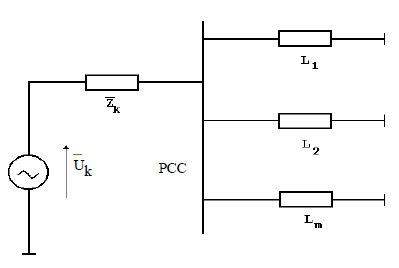
Fig.1. Single-phase representation of a power system with multiple loads connected to the same Point of Common Coupling (PCC) fed by a sinusoidal non-ideal generator.

As far as the “loading quality” and the “supply quality” are concerned, recommendations have been issued by the Standard Organizations both to limit the injection of harmonics [1 – 4] and to define the characteristics of the voltage supplied by public networks [5 – 7]. Definitions of power-quality related terms are also given [8]. However, these recommendations appear to be still insufficient to ensure the solution of the “power quality” problems. In fact, it should be considered that, when the supply voltage is distorted (and possibly unbalanced, in three-phase systems), a customer may not be totally responsible for the harmonic and unbalance current components flowing in its loads. Ethical and legal issues, other than technical ones, are involved, when setting allowable limits [9], since the source responsible for injecting the disturbances should be first of all detected.

The main issue, when dealing with “power quality”, is therefore that of detecting the source, or the sources, injecting the disturbances and quantifying the effect of such disturbances on the power quality. The next sections will discuss the technical respects of this problem, both from the methodological point of view and that of the measuring equipment.

2. THEORETICAL BACKGROUND

The power theory of the ac electric systems and circuits has developed, during the last century, under the strong constraint of sinusoidal waveforms. When disturbances are superimposed to the sinusoidal voltage and current waveforms, and particularly when such disturbances are steady-state disturbances, that constraint cannot be considered any longer. Consequently, all conventional quantities and factors usually employed in the energy characterization of the electric systems under sinusoidal conditions, such as the reactive and apparent powers and the power factor, lose most of the properties they have under sinusoidal conditions. This leads to a dramatic and misleading loss of information [10] when they are used in power-quality assessment.

In order to avoid these problems, the non-sinusoidal conditions should be theoretically reconsidered, starting from the mathematical bases of the electromagnetism and circuit theory, in order to describe the physical behaviour of an electric system under non-sinusoidal conditions in terms of a suitable set of equations and mathematical relationships that relate voltages, currents and physical properties of the system elements. At the Author’s knowledge, very few attempts have been published that try to give a general answer to this basic problem[11-13].

Nevertheless, several attempts were made, in the past, to extend to the non-sinusoidal systems concepts and definitions typical of the sinusoidal systems [14-18]. These attempts were mainly concerned with the solution of particular problems, typically the compensation of non-active current components and, in some cases, have been proved to be not totally correct from the physical point of view [19].

More recently, a more in-depth investigation into the power phenomena has been proposed by several Authors [12, 13, 21- 31], so that these phenomena are now more clearly described than in the past, although a generally accepted, comprehensive theory of the power phenomena under non-sinusoidal conditions is not yet available. A good, extensive survey of the scientific work done in this field is represented by the issues of the ETEP journal [32-36] dedicated to the contributions presented during five “International Workshops on Power Definitions and Measurements under Non-Sinusoidal Conditions” (Como, Italy, 1991, Stresa, Italy, 1993, Milano, Italy, 1995, 1997 and 2000).

A second critical point that must be considered when discussing about power quality measurement regards the evaluation of the measurement uncertainty in the presence of heavily distorted signals. Up to a recent past, only the behaviour of the active and reactive energy meters in the presence of distorted waveform conditions was widely discussed [37-39]. However, the power quality indices that have been more recently proposed require complex measuring systems for their measurement. The evaluation of the measurement uncertainty, according to the recommendation of the ISO Guide [40], is still an open problem.

All above referenced contributions represent a theoretical background wide enough, if properly applied, to allow a correct approach to power-quality definition and measurement.

3. POWER-QUALITY INDICES

The first, obvious, though not easy step towards power quality measurement is the definition of power-quality indices able to quantify the deviation from an ideal reference situation, quantify the detrimental effects of this deviation and identify the source generating these detrimental effects.

A quite natural way seems to be the extension to the non-sinusoidal conditions of the indices employed under sinusoidal conditions, such as the power factor and the Total Distortion Factor (THD), together with a discussion of their limits when the sinusoidal conditions are left.

In order to extend the definition of the power factor, the apparent power must be considered too. Its extension to the non-sinusoidal conditions is quite immediate for single-phase systems; on the contrary, several different definitions are available in the literature [41] when three-phase systems are considered. The following one, due to Buchholz [42], is receiving increasing acceptance in the scientific community, though it is not endorsed by several Standards:

.

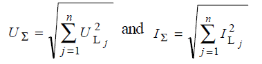
where UΣ and IΣ are the voltage and current collective rms values respectively and are defined as:
.

ULj and ILj being the rms values of the zero-sum line voltages and the line current respectively, n the number of wires of the system. If the total active power is defined as:

.

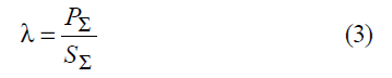
where T is the period of the voltage and current waveforms, the power factor can be still defined as the ratio between the active power and the apparent power (1):
.

The power factor (3) can be still considered a power-quality index, though it loses the property of fully qualifying the load. Under non-sinusoidal conditions it only represents an index of conformity of the line current waveforms to the line voltage waveforms.

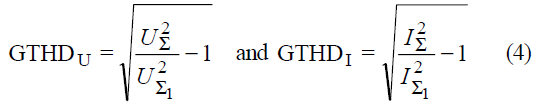
It can be easily proven that also the Distortion Factors only show the conformity of the line voltages and currents to sinewaves. In fact, for the three-phase systems, the global voltage and current THD factors can be defined as:
.

where UΣ1 and IΣ1 are the collective rms values of the fundamental frequency components of the line voltages and currents respectively. According to the given definition, factors (4) act as nonconformity indices of the line voltage and current waveforms to sinewaves, no matter if these sinewaves are balanced or not.

Since it has been proven that the harmonic components and the sequence components, in three-phase systems, have similar effects from the power-quality point of view and can be considered as the components of a generalized Fourier decomposition [28], the factors defined in (4) can be modified, in order to keep into account the effects of the unbalance components too, as:

.

where UΣ+1 and IΣ+1 are the collective rms values of the fundamental frequency, positive sequence components of the line voltages and currents respectively.

It can be readily checked that the factors defined in (5) act as nonconformity indices of the line voltage and current waveforms to positive sequence sinewaves.

The comparison between the values assumed by (4) and (5) allows to establish whether the responsibility for the electrical pollution is mostly due to the presence of distortion or to the presence of unbalance.

All above quantities, however, are not useful in establishing whether the load or the supply are responsible for the power quality deterioration, since they can only provide an estimate of conformity to given reference conditions, where, according to [1- 9], the term “conformity” denotes “the fulfilment of specified requirements”.

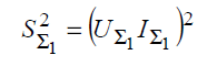
An attempt to find more useful indices has been proposed by the IEEE Working Group on Non-sinusoidal Situations [39] with the following resolution for the apparent power (1):

.

where UΣH and IΣH are the collective rms values of the harmonic components of voltage and current respectively.

Although the quantities:
.

and:

.

are introduced, it can be immediately checked that:

.

This approach, therefore, does not provide any additional information to the one associated with the THD factors and is useless in identifying the sources producing distortion.

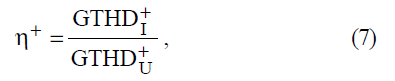
Some information about the location of the source producing distortion is provided by the ratio:
.

since a linear, balanced load is expected not to amplify the distortion of the current, with respect to that of the voltage, whilst a non-linear or unbalanced load is expected to. However index (7) is sensitive to resonance too, so it cannot discriminate between distortion and resonance effects.

The search for more effective approaches has led, recently, to focus on the analysis of the energy flowing in a network section [22, 43]. This analysis shows that, under distorted conditions, active power components associated with the harmonic and negative sequence components of voltages and currents arise that flow backward from the load to the generator, and dissipate in the generator source impedance. This phenomenon can be explained by considering the non-linear loads as “converters”, which draw active power at the fundamental frequency and positive sequence, and give back part of it at different frequencies and sequences.

According to the above considerations, the active power PΣ in the metering section of a three-phase circuit can be resolved as:

.

PΣ+1 is the active power generated by the sinusoidal, balanced ideal supply. The other terms in (8) represent active powers delivered to the load and generally dissipated if the supply is distorted and/or unbalanced, or reflected backward and dissipated in the equivalent source impedance if the load is non-linear, time-variant and/or unbalanced.

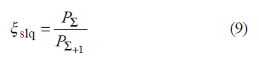
A first supply and loading quality index can be hence defined as [44]:
.

It can be readily checked that, when the distortion and/or unbalance of the supply prevail over the load distorting and unbalancing effects, ξslq > 1. On the contrary, when the load distorting and/or unbalancing effects prevail over the supply voltage distortion and/or unbalance, ξslq < 1.

A second power-quality index has been proposed [45]:
.

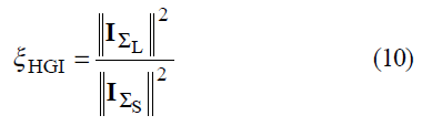
where IΣL is the vector of the collective rms values of the harmonic and sequence components associated with active powers reflected backward from the load to the source, and IΣS is the vector of the collective rms values of the harmonic and sequence components associated with active powers flowing from the source towards the load. The higher is the value assumed by (10), the higher is the load contribution to distortion.

Both indices (9) and (10) may provide incorrect information under practical conditions [46] when compensation effects arise between the harmonic power components injected by the supply and those reflected by the load and when the harmonic active powers are close to zero, due to a phase shift close to π/2 between the harmonic components of voltage and current, despite the presence of large harmonic current components.

Providing incorrect indications is a common flaw of all synthetic indices obtained from measurements done in a single metering section. These indices are somehow doomed to fail, since an electric system under non-sinusoidal conditions has a theoretically infinite number of freedom degrees [11], and therefore its state cannot be fully determined by means of a single index or quantity.

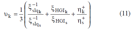
In order to overcome this problem, a new index has been recently proposed [47, 48], based on multi-point measurements of indices (7), (9) and (10). For each line k leaving a PCC, this index can be defined as:
.

where subscript k refers to a line leaving the PCC and subscript s refers to the line supplying the PCC.

This index is based on the consideration that, when indices ξHGI and η+ are evaluated for each line connected to the same PCC, the ratio of one index measured on one of the lines leaving the PCC with the same index measured on the line supplying the PCC increases if the disturbances are injected by the load connected to the line, while it decreases if the disturbances are injected by the supply. The opposite occurs when the ratio of indices ξslq is considered.

Index (11) averages the above ratios, and is expected to compensate the different reasons that cause each single index to fail in assessing the responsibility for the injection of disturbances. When υk > 1, the load connected to line k is injecting disturbances in the network. When υk < 1, line k is disturbed.

The capability of index (11) to identify the sources producing distortion and quantify the amount of injected disturbances has been tested both theoretically, by simulating its evaluation on the IEEE industrial test system proposed by the IEEE Task Force on Harmonic modelling and simulation [48] and experimentally, by means of measurements carried out on a small low-voltage network, supplying the machine shop of the Department of Electrical Engineering of the Politecnico di Milano University [47].

Figs. 2a and 2b show the schematic of this network and the plot of index (11) tracked for about 3 hours, under different operating conditions of the network. The location of the measuring systems is shown by the S blocks in the schematic of Fig. 2a. Both the simulation and experimental results appear quite interesting and encourage to further investigate the multi-point measurement approach.

4. THE MEASUREMENT PROBLEMS

Up to the present days, the discussion about power quality in the electric systems under non-sinusoidal conditions has dealt mainly with the definition of suitable theoretical approaches and indices. This is quite natural since, before measuring anything, the exact meaning of what is going to be measured should be understood.

Fig.2. The low-voltage network employed in the experimental tests (a), and the measured values for index (11) (b).

When the practical issues of measuring the defined quantities and indices began to be considered, it was soon clear that the traditional instruments (mainly active and reactive energy meters) used under sinusoidal conditions to evaluate the energy consumption, both from a quantitative and “qualitative” point of view, were inadequate [37, 38].

This inadequacy involves also the traditional electromagnetic current and voltage transformers, as well as the capacitive voltage transformers, used in High Voltage systems, whose bandwidth is too narrow to allow a correct transduction of the distorted signals.

This problem can be overcome, if the electronic transducers are used, based on zero-flux current transformers for the current transducers, and electro-optical techniques for the voltage transducers [49-51]. Several solutions have been proposed and are already commercially available.

As far as the measurement method is concerned, most of the newly defined indices, such as (7), (9), (10) and (11), require an extensive processing of the input signals to be determined: index (10), for instance, requires a Fourier Transform of both voltages and currents, and the evaluation of the active power associated with each voltage and current component. This kind of processing can be obtained only if the new, modern, DSP-based instruments are employed.

From a mere technical point of view, this is not a problem, since the available DSP-based structures perform the Analog-to- Digital conversion and the subsequent digital processing fast enough to allow a real-time evaluation of all above mentioned indices with the required resolution. Distributed measurement systems can be also implemented in a relatively simple way, so that the evaluation of indices based on multi-point measurements, such as (11), can be obtained [47].

The most critical problem, with the DSP-based systems that process complex measurement algorithms, is the uncertainty estimation. At this stage of the research on the electric systems under non-sinusoidal conditions, this is not only a mere metrological problem, but has also a large implication on the theoretical analysis. In fact, it should be always kept into account that no information can be obtained about the practical utility of any proposed theory until the defined quantities can be measured and the measurement uncertainty is known. In other words, the validity of any theoretical approach that is aimed at identifying a physical phenomenon and providing quantitative information about it is limited by the uncertainty with which the quantities employed to describe that phenomenon can be measured.

The reference document for expressing the uncertainty in measurement is the well known ISO Guide [40]. The Guide follows a probabilistic approach to the uncertainty, where the uncertainty itself is expressed as a standard deviation. In the recent years, this approach has been more and more questioned, since its application may become quite troublesome when the uncertainty of measurement based on complex DSP algorithms has to be estimated.

Several proposals are available in the recent literature to overcome this kind of problems. Some of them are still based on a probabilistic approach [52-55], while some others are looking for different, innovative mathematical approaches, such as the theory of the evidence and the fuzzy mathematics [56-59].

All the mentioned approaches are too complex to be considered in this short survey. It is however worth while to note that the research activity in the measurement field is eagerly considering the power-quality measurement problems and the characterization of the power-quality instruments as a challenging problems, and several answers have already been provided.

5. CONCLUSIONS

The considerations reported in the above sections allow for drawing a few conclusions about the present achievements and the future trends in the field of power-quality monitoring.

• The theoretical background is wide enough to allow a good analysis of the power quality in the presence of non-sinusoidal conditions, although a generally accepted approach for describing the behaviour of the electric systems under non-sinusoidal conditions has not yet been developed.

• Several indices have been proposed to detect the deviations from the reference ideal conditions that lead to power-quality problems.

• The analysis of the direction of the active power components associated with the harmonic and sequence components of voltages and currents has been proposed as the most effective tool for the identification of the sources producing distortion and unbalance.

• The use of a single index was proved to be not sufficient for power-quality assessment. The most recent developments of the research activity are oriented towards the use of indices obtained from multi-point measurements performed in different metering sections of the electric system.

• The presently available digital instrumentation is suitable for measuring the newly defined quantities and indices with good accuracy and at a reasonable cost.

• The true present challenge, is making the measurement uncertainty evaluation of the DSP-based instrument less troublesome than it presently appears if the recommendations of the ISO Guide [40] are strictly applied.

REFERENCES

[1] IEEE Standard 519-1992, IEEE Recommended practices and requirements for harmonic control in electrical power systems.
[2] IEC 61000-3-2, Electromagnetic compatibility (EMC) – Part 3-2: Limits – Limits for harmonic current emissions (equipment input current <= 16 A per phase), 1998.
[3] IEC 61000-3-4, Electromagnetic compatibility (EMC) – Part 3-4: Limits – Limitation of emission of harmonic currents in low-voltage power supply systems for equipment with rated current greater than 16 A, 1998.
[4] IEC 61000-3-6, Electromagnetic compatibility (EMC) – Part 3: Limits – Section 6: Assessment of emission limits for distorting loads in MV and HV power systems, 1996.
[5] IEC 61000-3-3, Electromagnetic compatibility (EMC) – Part 3-2: Limits – Limitation of voltage fluctuations and flicker in low-voltage supply systems for equipment with rated current <= 16 A, 1994.
[6] IEC 61000-3-5, Electromagnetic compatibility (EMC) – Part 3: Limits – Section 5: Limitation of voltage fluctuations and flicker in low-voltage power supply systems for equipment with rated current greater than 16 A, 1994.
[7] EN 50160, Voltage characteristics of electricity supplied by public distribution systems, CENELEC November 1994.
[8] IEEE Standard 1159-1995, IEEE Recommended practice for monitoring electric power quality.
[9] A.J. Berrisford, “Should a utility meter harmonics?”, Proc. of the IEE 7th CMATES, November 1992, Glasgow, U.K., IEE Conf. Pub. n. 367, pp. 86-89.
[10] G. Carpinelli, A. Testa, “Power quality indices and loss of information risk”, IMEKO TC-4 Symposium on Development in Digital Measuring Instrumentation, Naples, Italy, 1998.
[11] L. S. Czarnecki, “Power theory of electric circuits: common data base of power related phenomena and properties”, ETEP, vol. 4, n.6, 1994.
[12] Z. Čakareski, A. Emanuel, “Poynting vector and the quality of electric energy”, ETEP, vol. 11, n. 6, 2001.
[13] A. Ferrero, S. Leva, A. P. Morando, “An approach to the non-active power concept in terms of the Poynting-Park vector”, ETEP, vol. 11, n. 5, 2001.
[14] C. I. Budeanu, “Puissances reactives et fictives”, Inst. Romain de l’Energie, Bucharest, Rumania, 1927.
[15] S. Fryze, “Active, reactive and apparent power in circuits with non sinusoidal voltage and current”, (in Polish), Przegl. Elektrotech. , n.7; ibid., n. 8, 1931; ibid., n. 22, 1932.
[16] W. Shepherd, P. Zakikhani, “Suggested definition of reactive power for nonsinusoidal systems.”, Proc. Inst. Elec. Eng., vol. 119, and vol. 120, 1973.
[17] D. Sharon, “Reactive power definitions and power-factor improvement in nonlinear systems”, Proc. Inst. Elec. Eng., vol. 120, 1973.
[18] N. L. Kusters, W. J. M. Moore, “On the definition of reactive power under nonsinusoidal conditions”, IEEE Trans. Power App. Syst., vol. PAS-99, 1980.
[19] L. S. Czarnecki, “What is wrong with the Budeanu concept of reactive and distortion power and why it should be abandoned”, IEEE Trans. Instr. Meas., vol. 36, 1987.
[20] L. S. Czarnecki, “Considerations on the reactive power in nonsinusoidal situations”, IEEE Trans Instr. Meas., vol. 34, 1985.
[21] L. S. Czarnecki, “Orthogonal decomposition of the currents in a 3-phase nonlinear asymmetrical circuit with a nonsinusoidal voltage source”, IEEE Trans. Instr. Meas., vol. 37, 1988.
[22] L. S. Czarnecki, “Current and power equations at bidirectional flow of harmonic active power in circuits with rotating machines”, ETEP, vol. 3, n. 1, 1993.
[23] M. Depenbrock, “Quantities of a multiterminal circuit determined on the basis of Kirchhoff’s laws”, ETEP, vol. 8, n. 4, 1998.
[24] H. Akagi, Y. Kanazawa, A. Nabae, “Instantaneous reactive power compensators comprising switching devices without energy storage components”, IEEE Trans. on. Ind. Appl., vol. IA-20, n. 3, 1984.
[25] L. Rossetto, P. Tenti, “Evaluation of instantaneous power terms in multi-phase systems: techniques and applications to power conditioning equipment”, ETEP, vol. 4, n. 6, 1994.
[26] J. L. Willems, “A new intepretation of the Akagi-Nabae power components for nonsinusoidal three-phase situations”, IEEE Trans. on Instr. and Meas., vol. 41, n. 6, 1992.
[27] J. L. Willems, “Mathematical foundations of the instantaneous power concepts: a geometrical approach”, ETEP, vol. 6, n. 5, 1996.
[28] A. Ferrero, G. Superti-Furga, “A new approach to the definition of power components in three-phase systems under nonsinusoidal conditions”, IEEE Trans. on Instr. and Meas., vol. 40, n. 3, 1991.
[29] L. Cristaldi, A. Ferrero, G. Superti-Furga, “Power and current decomposition into time- and frequency-domain components: analysis and comparison”, ETEP, vol. 4, n. 5, 1994.
[30] L. Cristaldi, A. Ferrero, “Mathematical foundations of the instantaneous power concepts: an algebraic approach”, ETEP, vol. 6, n. 5, 1996.
[31] A. Ferrero, L. Giuliani, J. L. Willems, “A new space-vector transformation for four-conductor systems”, ETEP, vol. 10, n. 3, 2000.
[32] 1st Int. Workshop on Power Definitions and Measurements under Non-Sinusoidal Conditions, ETEP, vol. 3, n. 1, 1993.
[33] 2nd Int. Workshop on Power Definitions and Measurements under Non-Sinusoidal Conditions, ETEP, vol. 4, n. 5 and n. 6, 1994.
[34] 3rd Int. Workshop on Power Definitions and Measurements under Non-Sinusoidal Conditions, ETEP, vol. 6, n. 5 and n.6, 1996.
[35] 4th Int. Workshop on Power Definitions and Measurements under Non-Sinusoidal Conditions, ETEP, vol. 8, n. 4 and n. 5, 1998.
[36] 5th Int. Workshop on Power Definitions and Measurements under Non-Sinusoidal Conditions, ETEP, vol. 11, n. 5 and n. 6, 2001, and vol. 12, n.1, 2002.
[37] P.S. Filipski, R. Arsenau, “Behavior of wattmeters and watthour meters under distorted waveform conditions”. IEEE Tutorial Course, 90EH0327-7PWR, 1991.
[38] R. Arsenau, P.S. Filipski: “The effects of nonsinusoidal waveforms on the performance of revenue meters”. IEEE Tutorial Course, 90EH0327-7PWR, 1991.
[39] IEEE Working Group on Nonsinusoidal Situations, “Effects on meter performance and definitions of power: Practical definitions for powers in systems with nonsinusoidal waveforms and unbalanced loads: a discussion”, IEEE Trans. Pow. Del., vol.11, n.1, 1996.
[40] IEC-ISO Guide to the Expression of Uncertainty in Measurement, 1992.
[41] P. S. Filipski, R. Arseneau, “Definitions and measurement of apparent power under distorted waveform conditions”, IEEE Tutorial Course on Nonsinusoidal Situations, Course Text 90EH0327-7-PWR, pp. 37-42.
[42] F. Buchholz, “Die Drehstrom-Scheinleistung bei ungleichmäßiger Belastung der drei Zweige”, Licht u. Kraft, Org. Elektrotech. Ver. München, 1922, n. 2, pp. 9-11.
[43] P. H. Swart, M. J. Case, J. D. van Wyk, “On techniques for localization of sources producing distortion in three-phase networks”, ETEP, vol. 6, n. 6, pp. 391-396, 1996.
[44] A. Ferrero, A. Menchetti, R. Sasdelli, “Measurement of the electric power quality and related problems”, ETEP, vol. 6, n. 6, pp. 401-406, 1996.
[45] C. Muscas, “Assessment of electric power quality: indices for identifying disturbing loads”, ETEP, vol. 8, n.4, 1998.
[46] A. P. J. Rens, P. H. Swart: “On techniques for the localization of multiple distortion sources in three-phase networks: time-domain verification”, ETEP, Vol. 11, No. 5, 2001.
[47] L. Cristaldi, A. Ferrero, S. Salicone, “A Distributed System for Electric Power Quality Measurement”, IEEE Trans. Instr. Meas., vol. 51, n. 4, August 2002.
[48] D.Castaldo, A. Ferrero, S. Salicone, A. Testa, “A power-quality index based on multi-point measurements”, Proc. IEEE Power Tech 2003, Bologna, Italy, June 23-26, 2003.
[49] L. Cristaldi, A. Ferrero, M. Lazzaroni, R. Ottoboni, “A linearization method for commercial Hall-effect current transducers”, IEEE Trans. Instr. Meas., vol. 50, n. 5, 2001.
[50] A. Ferrero, R. Ottoboni, “A new low-cost voltage-to-voltage transducer for distorted signals”, IEEE Trans. on Instr. and Meas., vol. 47, n. 2, 1998.
[51] C. Svelto, R. Ottoboni, A. Ferrero, “Optically supplied voltage transducer for distorted signals in High-Voltage systems”, IEEE Trans. on Instr. and Meas., vol. 49, n. 2, 2000.
[52] G. Betta, C. Liguori, A. Pietrosanto, “Structured approach to estimate the measurement uncertainty in digital signal elaboration algorithms”, IEE Proc. Sci. Meas. Technol., vol. 146, n.1, 1999.
[53] G. Betta, C. Liguori, A. Pietrosanto, “Propagation of uncertainty in a discrete Fourier transform algorithm”, Measurement 27 (2000).
[54] A. Ferrero, M. Lazzaroni, S. Salicone, “A calibration procedure for a digital instrument for electric power quality measurement”, IEEE Trans. Instr. Meas., Vol. 51, n. 4, August 2002.
[55] S. Nuccio, C. Spataro, “Approaches to evaluate the virtual instrumentation measurement uncertainty”, IEEE Trans. Instr. Meas., Vol. 51, n. 6, 2002.
[56] G. Mauris, L. Berrah, L. Foulloy, A. Haurat, “Fuzzy handling of measurement errors in instrumentation”, IEEE Trans. Instr. Meas., vol. 49, no. 1, 2000.
[57] A. Ferrero, S. Salicone, “An innovative approach to the determination of uncertainty in measurements based on fuzzy variables”, IEEE IMTC/02, Anchorage, AK, USA, May 21-23, 2002.
[58] A. Ferrero, S. Salicone, “The Random-Fuzzy Variables: a new approach for the expression of uncertainty in measurement”, Proc. IEEE IMTC/2003, Vail, CO, USA, May 20-22, 2003.
[59] R. Sasdelli, A. Ferrero, A. Menchetti, A. Ferrero, L. Peretto, “About the accuracy of some proposed procedures for revenue metering under nonsinusoidal unbalanced conditions”, ETEP, vol. 8, n. 5, 1998.


Author: Prof. Alessandro Ferrero, Dipartimento di Elettrotecnica, Politecnico di Milano, Piazza Leonardo da Vinci 32, 20133 Milano, Italy, Tel: +39-02-233993751, Fax: +39-02-23993703, e-mail: alessandro.ferrero@polimi.it


Source: XVII IMEKO World Congress, Metrology in the 3rd Millennium June 22−27, 2003, Dubrovnik, Croatia.

Enclosure-Less Six-Phase Induction Motor

Published by Maciej GWOZDZIEWICZ1, Piotr KISIELEWSKI2, Wroclaw University of Science and Technology (1), KISIELEWSKI Sp. z o.o. (2)


Abstract. The papers deals with six-phase 2 kW 2-pole induction motor without enclosure. The motor is made of laser-cut construction steel , electrical steel and copper sheets. Shaft, two flange cartridge bearing units are machined by the milling machine. Bearings, stator winding and insulation are standard. The goal of the work is experimental investigation of impact of failures of the supply or stator winding on the motor performances.

Streszczenie. Artykuł przedstawia 6-fazowy 2-biegunowy silnik indukcyjny o mocy 2 kW. Model fizyczny silnika wykonano z blach ciętych laserem. Celem pracy jest weryfikacja wpływu uszkodzeń zasilania lub uzwojenia stojana silnika na jego właściwości. (Bezkadłubowy 6-fazowy silnik indukcyjny).

Keywords: enclosure-less, six-phase, induction motor, stator failure, supply failure
Słowa kluczowe: silnik bezkadłubowy, 6 faz, silnik indukcyjny, uszkodzenia stojana, uszkodzenia zasilan

Introduction

Laser cutting technology is being increasingly popular in electric machines manufacturing [8]. It enables to realize almost arbitrary project. The cost of laser cutting are going to even with cost of machining technology. Furthermore, AC electric machines can be built without enclosure. Of course, it reduces stiffness of the machine but simultaneously it decreases thermal resistance.

FEM motor model

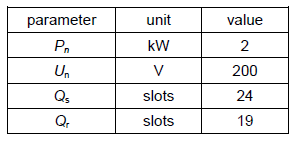
In Ansys Maxwell software 2D FEM 6-phase 2-pole induction motor field-circuit model was built [1-2]. Rated motor parameters are given in Table I.

Table 1. The parameters of the sensor

.

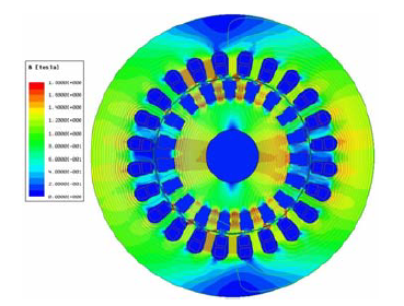
Stator double layer winding consists of 24 coils made of round double enamelled copper wire with coil pitch ys=5/6. Rotor winding consists of quasi-trapezoidal copper bars. Each rotor bar includes 2 rectangular copper bars with wider one at the bar top. Rotor slot openings are quite wide to decrease rotor winding leakage reactance and to obtain high starting and maximum motor torques. FEM motor model is presented in Fig. 1. Magnetic field distribution for rated load power is shown in Fig. 2.

Fig.1. FEM motor model
Fig.2. Magnetic field distribution in the motor model

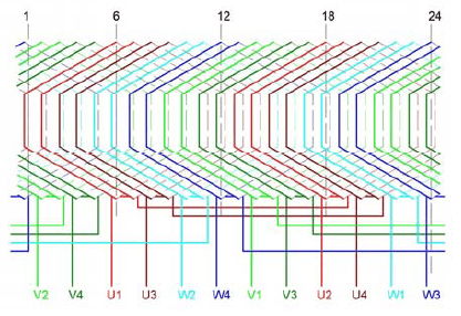
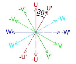
Motor is supplied by 6-phase sinusoidal voltage. The supply voltage consists of double 3-phase voltage with phase displacement equal to 30 degrees. Stator winding is connected in star [3-4]. Stator 6-phase winding distribution is given in Fig. 3. Supply 6-phase voltage vector diagram is presented in Fig. 4.

Fig.3. Stator 6-phase winding distribution
Fig.4. Supply 6-phase voltage diagram
Motor construction

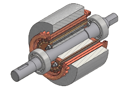
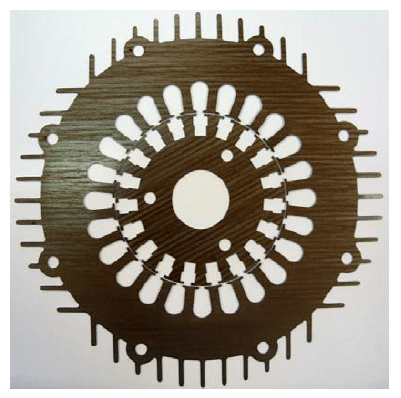
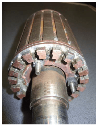
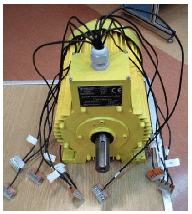
Stator and rotor sheets, rotor bars and rings and motor construction sheets are laser cut. Rotor rings connect bars and also keep rotor sheets due to 3 pressing rods. Motor construction is show in Fig. 5. Stator and rotors sheets are presented in Fig. 6. Stator sheets includes on the external edge cooling ribs and holes for pressing rods which keep the whole motor construction. The motor bearings type is 6205 2Z C3. Motor stator is presented in Fig. 7 and motor rotor is given Fig. 8. Finished motor is shown in Fig. 9.

Fig.5. Motor construction
Fig.6. Stator and rotor sheets
Fig.7. Stator before painting
Fig.8. Rotor
Fig.9. Finished motor
Experimental results

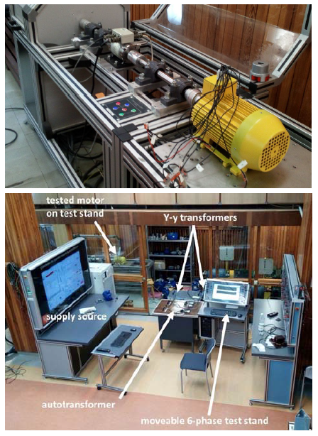
In laboratory of electric machines at Division of Electrical Machines and Measurements experimental investigation of designed and built enclosure-less 6-phase 2-pole motor was done. Test stand is presented in Fig. 10. Six-phase voltage was obtained by 3 transformers. Two of them were used to get double 3-phase voltage with phase displacement equal to 30 degrees. Additional third autotransformer was used to even RMS magnitude of all 6-phase voltages. Schema of the supply is presented in Fig. 11.

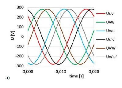
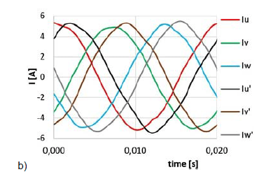
In the beginning, the motor was supplied by 6-phase voltage Un=200 V at rated frequency fn=50 Hz and loaded by rated load power Pn=2.0 kW. Voltage and motor current in time domain is given in Fig. 12. Comparison of the obtained experimental and simulation results is presented in Tab. 1.

Afterward, phase failures in the motor or supply were investigated [5-7]. The failures were simulated by switching-off one or more phase from the motor by circuit breakers which are shown in Fig. 13.

Fig.10. Test stand
Fig.11. Schema of the 6-phase supply
.
Fig.12. Six-phase a) voltage and b) current of the motor for rated load power
Fig.13. Circuit breakers simulating phase failures
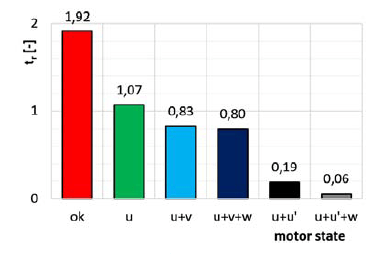
Fig.14. Impact of the phase failures on the motor breakdown torque
Fig.15. Impact of the phase failures on the motor starting torque

Firstly, influence of the phase failures on the motor breakdown torque was examined. Load torque was being increased with speed 10 Nm per 1 s. The results are given in Fig. 14. Next, influence of the phase failures on the motor starting torque was investigated. Supply voltage during measurement was equal to 80 V, starting torque value was referred to rated voltage Un=200 V. The results are presented in Fig. 15.

Table 2. Comparison of the obtained experimental and simulation results

.
Conclusions

Six-phase induction motor is very good alternative to three-phase induction motor due to much more reliability. In case of one-phase failure the motor performance enables motor to work. This solution can be very good proposition for traction electrical drives for which reliability is the most significant requirement.

It is possible to build enclosure-less electric motor for which almost all parts are made by laser cutting of steel, electrical steel and copper sheets. It is good alternative for standard motors with die-cast or welded enclosure.

Calculations have been carried out using resources provided by Wroclaw Centre for Networking and Supercomputing (http://wcss.pl), grant No. 400.

REFERENCES

[1] Livadaru L., Bobu A., Munteanu A., Vîrlan B. and Simion A., FEM-based Analysis on the Operation of Three-Phase Induction Motor connected to Six-Phase Supply System. Part 1 – Operation under healthy conditions, 2017 International Conference on Electromechanical and Power Systems (SIELMEN), pp. 119-124, December 2017
[2] Livadaru L., Bobu A., Munteanu A., Vîrlan B. and Simion A., FEM-based Analysis on the Operation of Three-Phase Induction Motor connected to Six-Phase Supply System. Part 2 – Study on fault-tolerance capability, 2017 International Conference on Electromechanical and Power Systems (SIELMEN), pp. 125-130, December 2017
[3] Nanoty A.S. and Chudasama A.R., Design of Multiphase Induction Motor for Electric Ship Propulsion, 2011 IEEE Electric Ship Technologies Symposium, pp. 283-287, May 2011.
[4] Bernatt J. and Glinka T., Electric machines with 6-phase winding, Wiadomości Elektrotechniczne 12/2008, pp. 14-19, 2008
[5] Abdelwanis M.I. and Selim F., A Sensorless Six-Phase Induction Motor Driving a Centrifugal Pump System, 2017 Nineteenth International Middle East Power Systems Conference (MEPCON), pp. 242-247, December 2017
[6] Ai Y., Wang Y. and Kamper M.J., Torque Performance Comparison from Three-Phase with Six-Phase Induction Machine, Proceedingsofthe 2009 IEEE International Conference on Mechatronics and Automation, pp. 1417-1421, August 2009
[7] Hammad R.A., Dabour S.M. and Rashad E.M., Performance of a Six-Phase Induction Motor Fed from a Z-Source Inverter under Faulty Conditions, 2017 Nineteenth International Middle East Power Systems Conference (MEPCON), pp. 1333-1338, December 2017
[8] Wilczynski W., Influence of magnetic circuit production for their magnetic properties, J. Mater. Sci., 8(2003) ,No. 38, 4905– 4910, August 2003


Authors: Pd.D. Maciej Gwoździewicz, Electrical Engineering Faculty at Wroclaw University of Science and Technology, E-mail: maciej.gwozdziewicz@pwr.edu.pl, Ph. D. Piotr Kisielewski, KISIELEWSKI Sp. z o.o., internet address: http://www.kisielewski.pl, E-mail: office@kisielwski.pl


Source & Publisher Item Identifier: PRZEGLĄD ELEKTROTECHNICZNY, ISSN 0033-2097, R. 95 NR 6/2019. doi:10.15199/48.2019.06.26

Electric Power Quality Evaluation in the Presence of Electromagnetic Emissions

Published by Giovanni Cipriani, Rosario Miceli, Member, IEEE, Ciro Spataro Member, IEEE DEIM University of Palermo Palermo, Italy rosario.miceli@unipa.it; ciro.spataro@unipa.it , Giovanni Tinè, Member, IEEE ISSIA National Council of Research (CNR) Palermo, Italy


Abstract— The measurements for the assessment of the electric power quality are often carried out in hostile electromagnetic environments. The aim of the paper is analyzing if and how both radiated and conducted electromagnetic emissions can disturb the measurement system used to quantify these disturbances. To achieve the target, an experimental approach is proposed, which, by means of a simple and fast test, allows establishing if the real electromagnetic environment, where power quality analysis is performed, can alter the measurements.

Keywords-electromagnetic immunity; power quality analysis

1. INTRODUCTION

In the electric power systems, determining and regulating the characteristics of both voltages and currents [1-5] is becoming more and more important, owing to the continuous increase of electric users susceptible to the variations of these characteristics respects to the rated ones [6-7]. In order to limit the injection of disturbances into the electric networks, there is the need to perform the evaluation of the so-called “electric power quality”; in many cases this evaluation is even prescribed by various national and international Standards and Laws.

Obviously, the power quality analysis must be often carried out in the proximity of the disturbance injection points (e.g. high power nonlinear loads, photovoltaic systems, fuel cells and wind generators) [8-14], where there is a high chance to utilize the measurement instrumentation in a hostile electromagnetic environment. The target of the paper is to establish if this environment can perturb the measurement instrumentation and alter the measurement results.

Due to complexity of the measurements, this kind of instrumentation is exclusively based on the analog-to-digital conversion of the electric signals and the successive processing of the acquired signals. In addition of the stand-alone power quality analyzers, more and more often, the measurements are performed using current and voltage probes, a general purpose data acquisition board connected to a common personal computer and processing (successively or in real time) the acquired data by using the computer processor itself [15-17].

This solution is less expensive respect to a stand-alone instrument and allows an easy updatability to the continuous variations of the rules prescribed by the Standards and the Laws concerning the electric power quality.

For the “stand-alone” electric power analyzers, usually characterized by the manufacturers themselves from the electromagnetic compatibility viewpoint, it is quite easy obtaining information about the levels of conducted or radiated disturbances that can alter their performances. On the contrary, with regard to more complex measurement systems, which are constituted of various components provided by different manufacturers, the analysis of their electromagnetic immunity degree is not simple. Even having access to the electromagnetic compatibility data of each component, the extension of these specifications to the whole measurement chain is not completely straightforward. The whole measurement system has to be considered as unique equipment under test. Only in this way, a complete characterization of the system from the electromagnetic compatibility viewpoint can be carried out.

To perform this characterization and to quantify the immunity degree of the measurement systems, it is necessary to choose one or more parameters that are representative of their performances and analyze if and how these parameters vary when the systems are subjected to electromagnetic disturbances.

In previous works [18-20], we showed that the parameters, sufficient to characterize an analog to digital conversion based measurement system are offset, gain, the total harmonic distortion (THD), the total spurious distortion (TSD) and the signal to noise ratio (SNR). Therefore, we used these five parameters to assess the electromagnetic immunity of the considered measurement systems.

In order to apply standard requirements and criteria for the immunity tests, we took into account the IEC-61236 standard [21] that specifies minimum requirements for immunity and emissions regarding electromagnetic compatibility for electrical equipment for measurement, control and laboratory use.

We performed an extensive series of experiments on various configurations of systems, varying the typology, the shielding conditions, the relative and absolute position of each component of the measurement chain and varying typology, amplitude and/or frequency of the electromagnetic disturbance.

By means of time and frequency analysis [22-23], we were able to assess, the electromagnetic immunity degree of a generic measurement system when it is subjected to the standardized disturbances prescribed in [21]. However, from the obtained data, we can not establish if, considering the real shielding and grounding conditions of the measurement chain, the actual and generally unknown electromagnetic environment, where the instrument will actually operate, is able to compromise its metrological characteristics. Therefore, our target is the definition of a procedure to assess the actual immunity degree to the unknown electromagnetic disturbances that are actually present in the place where the measurement is performed.

In the following we abridge the results obtained subjecting the systems to the tests advised in [21] (chapter II). In chapter III we propose the procedure to assess the immunity degree of the instruments in presence of unknown electromagnetic disturbances and in chapter IV this procedure is validated by applying it to various practical cases.

II. THE IEC-61236 STANDARD

The IEC-61236 standard [21] prescribes to subject the measurement system to the following electromagnetic phenomena: radiated radio-frequency disturbances; bursts; surges; conducted radio-frequency disturbances; voltage interruptions; electrostatic discharges; rated power frequency magnetic field. For each phenomenon the immunity requirements and limits are given for normal environments, industrial locations and for controlled electromagnetic environments. As for the instrumentation, setup and management of the experimental tests, we took into consideration the IEC-61000-4 series standards [24]. We considered the total measurement chain, constituted of cables, antialias filter, connector box, data acquisition board and personal computer, testing both full-shielded configurations and not-shielded configuration. In this framework we consider four different National Instrument data acquisition boards, whose technical characteristics are reported in table I.

TABLE I. CHARACTERISTICS OF THE TESTED BOARDS

.

The data acquisition boards are linked to a shielded connector box NI SCB68 through a shielded cable NI SCH6868 (1m). We tested also a not-shielded configuration linking the boards to a CB-68LP connector block trough a R6868 ribbon cable (1m). To link the measurement point to the various connector boxes, we use a RG-58 type coaxial cable (0.5 m) or a LMR0-600-DB double-shielded coaxial cable for the full-shielded configurations. Before the connector boxes is inserted an ad-hoc build IV order low-pass antialias filter.

The environment and the instrumentation used to generate the electromagnetic disturbances are full-compliant with [24].

As inputs for the tested systems, DC and sinusoidal signals are generated by the Agilent 33120A function and arbitrary waveform generator. All the measurements are performed in differential mode, sampling at the maximum rate.

In order to test the systems under radiated emissions, we performed various tests inside both a semi-anechoic chamber and a GTEM cell. radio-frequency fields with 1, 3, 10 V/m strength are irradiated towards the tested instruments, as prescribed in [21]. The disturbance frequency is incrementally swept in the frequency range 80 ÷ 1000 MHz with a 1% step size and the disturbance fields are 80% amplitude modulated with a 1 kHz sine wave [24]. All the tests were performed varying personal computers, data acquisition boards, cables and connector boxes of the tested systems, the reciprocal positions and orientations of these components and the frequency and strength of the disturbance fields.

In all cases, we observed that spurious frequencies arise during the signals acquisition [22]. These spurious components are a DC component, the disturbance modulating signal and its harmonics; in the prescribed frequency range, the disturbance carrier signal and its harmonics are completely filtered by the limited bandwidth of the tested instruments. In any case, mainly for the not-shielded configurations, the presence of these spurious frequencies reduces the TSD value and alters the offset value. By analyzing the acquired signals, we verified that the amplitude of the spurious frequency components (and consequently the coupling intensity and the immunity level) is: weakly depending on the data acquisition board, motherboard and case models and strongly depending on the shielding dress of cables and connector boxes; slightly depending on the personal computer and connector box position and strictly depending on the signal cables position; strictly depending on the disturbance strength, but not-depending on the disturbance frequency, except when the system resonates, allowing a much tighter coupling and strongly increasing the spurious frequencies amplitude.

As for the conducted disturbances, we started the experiments with the burst, which consists of a sequence of a limited number of distinct pulses whose characteristics are prescribed in [21].

Using the not-shielded configurations, during the burst injection into the supply cable, visible spikes, superimposed to the sinusoidal signal, appear causing a temporary variation of the offset and SNR values [22]. However we noticed that the acquired disturbance level depends on the reciprocal position of the signal cables and the supply cable, where the bursts are injected. This means that the disturbance injected in the supply cable produces an inductive interference with the measurement system. With the aim to quantify the inductive coupling mechanism, we tested a full-shielded configuration. With this arrangement, no effects are observed when the measurement system is subjected to the bursts; therefore, from this experiment, we can deduce that the coupling mechanism between disturbance and the measurement system is only inductive and only caused by the disturbance flowing in the supply cable [22]. To find another evidence of this thesis, we tested again the not-shielded configuration, but shielding the supply cable. Also in this way, the system is immune to the bursts.

Injecting into the supply cable a surge, which is a voltage pulse wave whose characteristics are prescribed in [21] and repeating the same methodology employed for the bursts, we obtained similar results, namely that the full-shielded configurations are practically immune to the surges, while with a not-shielded configuration the surges effects are manifestly visible on the acquired signals [22].

With the same methodology, we tested the effects of the conducted radio-frequency fields, injecting in the supply cable of the tested instruments 1 V and 3 V amplitude disturbances. The disturbance frequency is incrementally swept in the frequency range 80 ÷ 1000 MHz with a 1% step size and the disturbance signals are 80% amplitude modulated with a 1 kHz sine wave [21]. Once more the coupling mechanism between disturbance and the measurement system is only inductive and there are not conductive paths. Therefore, for the full-shielded configurations, no visible effects appear while a radiofrequency threat crosses the supply cable, and no variations of offset, gain and TSD values were observed. Repeating the experiments onto the not-shielded configuration, the emissions flowing in the supply cable couple with the measurement system and spurious frequencies arise during the signals acquisition. These spurious components are a DC component, the disturbance carrier signal and its harmonics and the disturbance modulating signal and its harmonics [22]. Of course some of these components can appear in their alias version or can be completely filtered, depending on the sampling frequency and on the instrument bandwidth. In any case the presence of these spurious frequencies reduces the TSD value and alters the offset value.

When the tested systems are subjected to 1-cycle supply interruptions, no visible effect appears during the signals acquisition, either with full-shielded configuration or with not-shielded configuration.

Contact and air discharges in both polarities were applied in various points of the measurement system, starting from 1 kV and increasing the test level value with a step size of 0.5 kV until reaching, as prescribed in [21], the 8 kV level. No visible effects were observed and therefore, with respect to the not-perturbed conditions, no changes were detected in the offset, gain, TSD and SNR values.

Eventually, the systems were subjected to 50 – 60 Hz magnetic field reaching the 30 A/m strength level prescribed for industrial locations. Also in this case, no effects were observed.

To perform the tests, we used the NI LabView programming language to drive the data acquisition boards, to process the acquired samples and to realise the user interface. During all the immunity tests, no faults of the software were detected, no system resets occurred and the measurement instruments kept on working without any loss of functions. Therefore, the software part of the instruments can be considered immune to all the electromagnetic emissions prescribed in the IEC 61326 standard.

The results of the tests can be summarized stating that, under the standard electromagnetic disturbances prescribed in [21] and mainly for the not-shielded configurations, the offset values can appreciably change and the TSD and SNR values can lower. Therefore, the standard uncertainties associated to these uncertainty sources can increase.

III. THE PROPOSED APPROACH

By analyzing the results of the tests, we are able to assess the immunity degree of a self-made power quality analyzer when it is subjected to the standardized disturbances prescribed in [21], deducing that the instrument performances can reveal perceptible degrade and, consequently, the uncertainty values can raise. However, from the obtained data, we can not establish if, considering the real shielding and grounding conditions of the measurement chain, the actual electromagnetic environment, where the instrument will actually operate, is able to compromise its metrological characteristics. Therefore, it could be useful to define a procedure which, by means of a desirably simple and fast test, allows the assessment of the actual immunity degree to the electromagnetic disturbances that are actually present in the place where the measurement is performed.

To outline this procedure, we started analyzing two interesting phenomena: we experimentally noticed that the disturbance effect is linearly added to the measurement signal (obviously excluding the cases which cause the A/D converter saturation and excluding the alias phenomena which however are avoided by the insertion of the low-pass filter). Moreover, we observed that, simultaneously applying various electromagnetic threats, the effects of these disturbances combine in an approximately linear way. Therefore, for whatever input signal, if it is known, it is possible to quantify the consequences produced by the actual electromagnetic conditions. It is clear that the more accurate and less expensive signal to use in order to perform the test is a 0 V DC signal.

It is enough, therefore, to close the measurement chain in short circuit and, by means of a time and/or frequency analysis, it is possible to evaluate if and how the real electromagnetic disturbances alter the offset, TSD and SNR values. Starting from this data and applying the method suggested in [20], we can estimate the actual measurement uncertainty and we can easily decide if, considering the target uncertainty, the considered instrument can still be adequately used in the electromagnetic environment where is performing the measurement.

If possible, better results can be obtained closing the measurement chain in an impedance equal to the one of measurement point.

In the cases of steady disturbances and if their effects are not within the bandwidth of interest of the measurement, it is possible to implement, into the software part of the instruments, algorithms to compensate for the disturbance effects.

IV. VALIDATION

In order to validate the proposed approach, we performed various measurements in locations where heavy, but unknown, electromagnetic disturbances were present.

Let us consider the AI 16XE10-50 data acquisition board inserted in the notebook with a not-shielded configuration operating in the nearness of a voltage source inverter working in steady conditions.

By means of this board, we build a system for DC, RMS and THD value measurement of a distorted 50 Hz voltage signal with the characteristics reported in row II of table II.

TABLE II. MEAN VALUES OF THE MEASURES PERFORMED NEARBY THE INVERTER

.

The signal is generated by the Agilent 33120A. The measurement is performed in differential mode, setting the gain to 1, sampling at 100 KS/s and choosing a 100 ms time window.

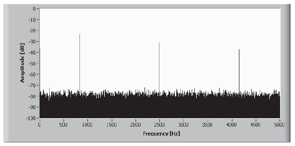
Before performing the measurements, we short circuited the measurement chain and we performed a frequency analysis, which is reported in fig.1.

Figure 1. Frequency analysis with short circuited measurement chain in the nearness of the voltage source inverter

The analysis show that the inverter is producing a visible interference with the system, generating a 15.5 mV DC component; a 831 Hz component and its III and V order harmonics. For the measurement at issue, these components will not alter the measured THD value, but will alter the measured RMS and DC value. Performing the measurement, in fact, we get the values reported in row III of tab. II (all the reported values are the means of 50 measurements).

Filtering the disturbance components and subtracting the DC value measured during the test, it is possible to correct the results, obtaining the data reported in row IV of tab. II.

In order to validate the used approach, we repeated the measurement turning off the voltage inverter, obtaining the values reported in row V of tab. II.

For this measurement, therefore, the impact of the voltage source inverter can be practically removed by implementing the appropriate compensation algorithm and the system can be safely used even with a not-shielded configuration.

Repeating the measurement with a full-shielded configuration and without the compensation algorithm, the inverter impact is almost completely negligible; in fact we obtained the value reported in row VI of tab. II.

The results obtained with the last experiment ensure that the electromagnetic disturbance has no effect on the signal generator.

We repeated the same measurement in the proximity of a 15 kVA welding machine. Before performing the measurements, we short circuited the measurement chain and we carried out a time and frequency analysis, which are respectively reported in fig.2 and in fig.3.

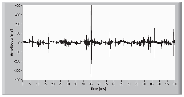
Figure 2. Time analysis with short circuited measurement chain in the
nearness of the welding machine

Figure 3. Frequency analysis with short circuited measurement chain in the
nearness of the welding machine

In this case, the electromagnetic disturbance produces a heavy and not steady interference with the instrument and therefore the repeatability of the measurement get worse. Moreover, the disturbance effect occupies the bandwidth of interest and therefore, in these electromagnetic environment conditions, it is not possible to correct the disturbance impact.

In table III the mean values and the standard deviations of 50 measurements are reported.

TABLE III. MEAN VALUES AND STANDARD DEVIATIONS OF THE MEASURES PERFORMED IN THE NEARNESS OF THE WELDING MACHINE USING THE NOT-SHIELDED CONFIGURATION

.

The same measurement was performed by using a full-shielded configuration and, in this case, the impact of the electromagnetic disturbance is greatly reduced (table IV).

TABLE IV. MEAN VALUES AND STANDARD DEVIATIONS OF THE MEASURES PERFORMED IN THE NEARNESS OF THE WELDING MACHINE USING THE SHIELDED CONFIGURATION

.

In this case, even though it is not possible to correct the disturbance effects and even though these effects are quite heavy, a good shielding allows a correct employment of the system.

Also the not-shielded configuration can be used if the uncertainty target is compatible with the uncertainty enhancement caused by the electromagnetic threat. To assess this enhancement, let’s consider that, on the average, the considered electromagnetic disturbance causes a 4 mV offset expansion and a 9 dB SNR reduction. Starting from this information and applying the method suggested in [20], it is possible to estimate the actual combined uncertainty.

The proposed approach can be easily extended to more complex measurement chains, such as when transducers and signal conditioning accessories are connected to a data acquisition board. Also in these cases, after having closed the measurement chain in short circuit, a time and/or frequency analysis allows to evaluate if and how much the actual electromagnetic disturbances can distort the measurement results.

For instance, let us consider the same board used in the previous examples. In order to perform a 230 V 50 Hz feed voltage RMS measurement in an industrial location where various welding machines and other metallurgic devices were operating, we connected to the board the differential high voltage probe Tektronics P5200 through an ad-hoc built IV order antialias filter with a 4 kHz cut-off frequency. The measurement is performed in differential mode, setting the probe attenuation ratio to 50 and the board gain to 1, sampling at 10 KS/s and choosing a 1 s time window. Let the standard uncertainty target be 0.5 %. Without electromagnetic disturbances, the instrument is safely capable to achieve this uncertainty. In order to evaluate the disturbance impact, before performing the measurements, we short circuited the measurement chain and we carried out a time analysis, which is reported in fig.4.

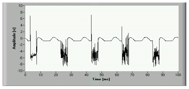
Figure 4. Time analysis with probe and short circuited measurement chain

The electromagnetic disturbances produce a heavy interference with the measurement instrument, which causes a 2.4 V RMS noise; since their effects occupy the bandwidth of interest of the measurement at issue, it is not possible to correct the disturbance impact. Since this noise cause a 14 dB SNR reduction, as a consequence, in the described electromagnetic environment the uncertainty target cannot be reached.

The experiments performed both under standardized disturbances and under unknown disturbances have shown that the full-shielded configurations of measurement systems are practically immune to the electromagnetic interferences. Even the heaviest radiated and conducted emissions cause a negligible impact if the good practices of shielded are observed.

However a full-shielded configuration of the whole measurement chain is quite expensive, since it is necessary to employ quite costly cables and connector boxes and the measurement shell be performed by skilled personnel.

We are investigating the chance to safely use the not-shielded configurations in a hostile electromagnetic environment, by the implementation of a procedure which allows the compensation of the disturbance effects.

The basic idea is established on a two channel acquisition technique. The measurement signal is sent to the first channel and, simultaneously, to the second channel, but with inverse polarity; the cable paths are arranged in a manner that the electromagnetic emissions induce the same effects on the two channels. Adding and dividing by two, via software, the data acquired by the two channels, we should obtain the measurement signal without the effect of the electromagnetic disturbances.

We are performing various tests to validate this technique and the first results are encouraging [25].

V. CONCLUSIONS

Starting from the experimental results obtained subjecting various configuration of systems to the electromagnetic disturbances prescribed in the IEC-61236 standard, in the paper we defined and proposed a simple and fast procedure to assess the actual impact of unknown electromagnetic disturbances on a measurement system for the electric power quality evaluation.

By means of this approach, it is possible to quantify the electromagnetic environment interference with the measurement systems and, therefore, to decide if the actual shielding conditions are adequate for the measurement purposes.

The application of this procedure has shown that the well-shielded configurations are virtually immune also to heavy disturbances.

As for the not-shielded configurations, the procedure allows the measurement correction when the measured typology is known and the disturbance effects are steady and not within the bandwidth of interest.

ACKNOWLEDGMENT This publication was partially supported by the PON04a2_H “i-NEXT” and PON01_02422 “SNIFF – Sensor Network Infrastructure For Factors” Italian research programs. This work was realized with SDESLab – University of Palermo.

REFERENCES

[1] G. Cipriani, G. Ciulla, V. Di Dio, D. La Cascia, and R. Miceli, “A device for PV modules I-V characteristic detection,” in Clean Electrical Power: Renewable Energy Resources Impact, 2013. ICCEP ’13. International Conference on, 2013.
[2] V. Di Dio, G. Cipriani, D. La Cascia, and R. Miceli, “Design, Sizing and Set Up of a Specific Low Cost Electronic Load for PV Modules Characterization,” in Ecological Vehicles and Renewable Energies (EVER), International Conference & Exhibition on, 2013.
[3] A. Ando, S. Mangione, L. Curcio, S. Stivala, G. Garbo, A. Busacca, G. M. T. Beleffi, and F. S. Marzano, “Rateless codes performance tests on terrestrial FSO time-correlated channel model,” in 2012 International Workshop on Optical Wireless Communications, IWOW 2012, 2012.
[4] A. C. Busacca, S. Stivala, L. Curcio, and G. Assanto, “Parametric conversion in micrometer and submicrometer structured ferroelectric crystals by surface poling,” International Journal of Optics, vol. 2012, 2012.
[5] M. Cherchi, S. Bivona, A. C. Cino, A. Busacca, and R. Oliveri, “Universal Charts for Optical Difference Frequency Generation in the Terahertz Domain,” IEEE Journal of Quantum Electronics, vol. 46, pp. 1009–1013, 2010.
[6] A. O. Di Tommaso, F. Filippetti, Y. Gritli, F., R. Miceli, and C. Spataro, “Double Squirrel Cage Induction Motors: a New Approach to Detect Rotor Bar Failures,” in 19th IMEKO TC 4 Symposium and 17th IWADC Workshop Advances in Instrumentation and Sensors Interoperability, 2013.
[7] A. O. Di Tommaso, F. Genduso, R. Miceli, and C. Spataro, “Voltage Source Inverters: an Easy Approach for Fast Fault Detection,” in 19th IMEKO TC 4 Symposium and 17th IWADC Workshop Advances in Instrumentation and Sensors Interoperability, 2013.
[8] G. Cipriani, V. Di Dio, D. La Manna, F. Massaro, R. Miceli, and G. Zizzo, “Economic Analysis on Dynamic Photovoltaic Systems in New Italian ‘Feed in Tariffs’ Context,” in Clean Electrical Power: Renewable Energy Resources Impact, 2013. ICCEP ’13. International Conference on, 2013.
[9] G. Cipriani, V. Di Dio, L. P. Di Noia, F. Genduso, D. La Cascia, R. Miceli, and R. Rizzo, “A PV Plant Simulator for Testing MPPT Techniques,” in Clean Electrical Power: Renewable Energy Resources Impact, 2013. ICCEP ’13. International Conference on, 2013.
[10] V. Di Dio, R. Miceli, C. Rando, and G. Zizzo, “Dynamics photovoltaic generators: Technical aspects and economical valuation,” in Power Electronics Electrical Drives Automation and Motion (SPEEDAM), 2010 International Symposium on, 2010, pp. 635–640.
[11] Boscaino, V., Pellitteri, F., Rosa, L., & Capponi, G. (2013). Wireless battery chargers for portable applications: design and test of a high efficiency power receiver. IET Power Electronics, 6(1), 20-29.
[12] V. Boscaino, R. Miceli, and G. Capponi,, MATLAB-based simulator of a 5 kW fuel cell for power electronics design, International Journal of Hydrogen Energy, Volume 38, Issue 19, 27 June 2013, Pages 7924-7934, ISSN 0360-3199
[13] V. Boscaino, R. Miceli, and G. Capponi, “A semi-empirical multipurpose steady-state model of a fuel cell for household appliances,” Proceedings of the International Conference on Clean Electrical Power: Renewable Energy Resources Impact, ICCEP 2013, 2013, pp. 1–6.
[14] V. Boscaino, P. Livreri, F. Marino, M. Minieri, Current-sensing technique for current-mode controlled voltage regulator modules, Microelectronics Journal, Volume 39, Issue 12, December 2008, Pages 1852-1859, ISSN 0026-2692.
[15] S. Caldara, S. Nuccio, and C. Spataro, “A virtual instrument for measurement of flicker,” IEEE Transactions on Instrumentation and Measurement, vol. 47, pp. 1155–1158, 1998.
[16] A. Cataliotti, V. Cosentino, D. Di Cara, A. Lipari, S. Nuccio, and C. Spataro, “A PC-based wattmeter for accurate measurements in sinusoidal and distorted conditions: Setup and experimental characterization,” IEEE Transactions on Instrumentation and Measurement, vol. 61, pp. 1426–1434, 2012.
[17] A. Cataliotti, V. Cosentino, D. Di Cara, A. Lipari, S. Nuccio, and C. Spataro, “A PC-based wattmeter for high accuracy power measurements,” in 2010 IEEE International Instrumentation and Measurement Technology Conference, I2MTC 2010 – Proceedings, 2010, pp. 1453–1458.
[18] S. Nuccio and C. Spataro, “Uncertainty management in the measurements performed by means of virtual instruments,” in AMUEM 2008 – IEEE Workshop on Advanced Methods for Uncertainty Estimation Measurement Proceedings, 2008, pp. 40–45.
[19] C. Spataro, “ADC based measurements: A common basis for the uncertainty estimation,” in 17th Symposium IMEKO TC4 – Measurement of Electrical Quantities, 15th International Workshop on ADC Modelling and Testing, and 3rd Symposium IMEKO TC19 – Environmental Measurements, 2010, pp. 389–393.
[20] C. Spataro, “ADC based measurements: Identification of the parameters for the uncertainty evaluation,” in 2009 IEEE International Workshop on Advanced Methods for Uncertainty Estimation in Measurement, AMUEM 2009, 2009, pp. 80–84.
[21] IEC 61326 “Electrical equipment for measurement, control and laboratory use – EMC requirements”, 2002.
[22] S. Nuccio, C. Spataro, and G. Tinè, “Immunity of a virtual instrument to radiated electromagnetic disturbances,” in Conference Record – IEEE Instrumentation and Measurement Technology Conference, 2003, vol. 1, pp. 780–784
[23] S. Nuccio, C. Spataro, and G. Tinè, “Immunity of a virtual instrument to conducted electromagnetic disturbances,” in Conference Record – IEEE Instrumentation and Measurement Technology Conference, 2004, vol. 3, pp. 1886–1890.
[24] IEC 61000-4-Series “Electromagnetic compatibility (EMC) – Part 4: Testing and measurement techniques”.
[25] S. Nuccio, C. Spataro, and G. Tinè, “Virtual instruments: Uncertainty evaluation in the presence of unknown electromagnetic interferences,” in AMUEM 2008 – IEEE Workshop on Advanced Methods for Uncertainty Estimation Measurement Proceedings, 2008, pp. 56–61.


Source: International Conference on Renewable Energy Research and Applications (ICRERA). Madrid, Spain, 20-23 October 2013.

An Analysis of Power Supply Reliability Indexes in the Selected Distribution Company

Published by Zbigniew ŁUKASIK, Jacek KOZYRA, Aldona KUŚMIŃSKA-FIJAŁKOWSKA,
Uniwersytet Technologiczno-Humanistyczny w Radomiu, Wydział Transportu i Elektrotechniki


Abstract. The main goal of this article was to present the problem of discontinuity of energy supply and methods applied by selected distribution company in order to improve power supply reliability indexes. An analysis of discontinuity of supply was based on data obtained from selected department of a distribution company with six energy areas. Based on these data, the impact of the investments, repairs, random events and other factors on the value of power supply reliability indexes was presented.

Streszczenie. Głównym celem publikacji jest przedstawienie problemu nieciągłości dostarczania energii elektrycznej oraz metod stosowanych przez wybraną spółkę dystrybucyjną w celu poprawy wskaźników niezawodności zasilania. Analizę nieciągłości zasilania zawartą w pracy oparto o dane pozyskane z wybranego oddziału spółki dystrybucyjnej (OSD), na terenie którego działa sześć rejonów energetycznych. Na podstawie danych przedstawiono wpływ inwestycji, remontów, zdarzeń losowych oraz innych czynników na wartość wskaźników niezawodności zasilania. (Analiza wskaźników niezawodności zasilnia w wybranej spółce dystrybucyjnej).
Słowa kluczowe: Spółka dystrybucyjna, System elektroenergetyczny, SAIDI, SAIFI.
Keywords: Distribution company, Power system, SAIDI, SAIFI.

Introduction

Power cut is defined as the state when energy is not available for a consumer in a place defined in an agreement. While supervising continuity of energy supplies and describing them using indexes, it is important to determine exact time of occurring power cut [1-5]. There are some minor but significant differences in defining and classifying power cuts [6-8]. In practice, there are two definitions of power cut. Although the effect of power cut is the same in most cases, the definition resulting from both definitions is important. The first definition uses the value of voltage at a place of connecting the consumer to the network. If the value of voltage is zero or close to zero, such state is defined as power cut. The practical implementation of this definition requires monitoring of voltage in all places of connecting the consumers. Collecting so many data using available technologies requires large financial outlays and that’s why it is economically unjustified.

The second definition is based on the notion of galvanic connection between the main part of electrical power system and consumer. If there is no galvanic connection between the consumer and main part of network, such state is called power cut. This definition does not directly match the feelings of a consumer, but its application for the purposes of collection of data about continuity of energy supplies is much easier for a network operator. Opening the connector that causes power cut often happens automatically and it is not always registered at low voltage. Manual closing of a connector is often a basis for statistics of continuity of energy supplies. At the highest levels of voltage, the systems of data collection and SCADA are usually applied to register power cuts.

The actions taken to improve power supply reliability indexes in the distribution networks

In the power industry, the key element improving power supply reliability indexes is increasing financial outlays for modernization and replacement of electrical power equipment, exploited lines and devices. Financial expenditures on replacement modernization and increasing resistance of low-voltage and medium-voltage network on atmospheric phenomena constituted in the years 2014 – 2017 nearly 40% of all expenditures of the operators of the distribution company system on the investments [17,18]. In many cases, the expenditures on the investments and renovation works in the distribution enterprises on particular elements of an electricity grid did not meet the needs. To ensure proper technical state and improve power supply reliability indexes, constant modernization and successive replacement of particular elements of distribution networks are required [9-14]. For this purpose, the actions in three key elements of distribution networks are taken:

Medium-voltage lines

– The replacement of bare conductors with insulated ones,
– The construction of medium-voltage and low-voltage double voltage lines on one supporting structure,
– The replacement of overhead medium-voltage string lines with cable lines,
– The application of high-quality fittings – poles, insulators, fixing wires,
– Tree cutting for medium-voltage lines,
– The automation of medium-voltage network,
– Installing short-circuit current flow indicators,
– The systems of automatic supply restoration of medium-voltage network – Fault Detection, Isolation and Restoration (FDIR).

Low- and medium-voltage transformer stations

– The application of modern solutions of simplified and small-sized stations,
– The application of integrated digital security systems,
– The use of switches with vacuum insulation or SF6.

Low-voltage lines

– The replacement of low-voltage overhead lines with insulated lines,
– The works on the line in technology of live working,
– The replacement of poles and insulators.

Another action taken to improve power supply reliability indexes in the distribution companies is also monitoring of electricity grid [15,16]. The programs such as SCADA WindEx are used. System provides data reading on the synoptic model and computer screen. The simulation environments are also applied to determine reliability rates of distribution network cooperating closely with SCADA systems such as WindEx AWAR. Program of monitoring vehicles, FLOTA has been applied and it is an additional tool for a dispatcher to get to a place of failure faster.

An analysis of SAIDI in selected energy areas of the distribution company

In the discussed department of distribution company, there are six energy areas of different territorial structure and various distribution of the consumers in the rural and urban areas. The indexes obtained from two energy areas contained in G-10,5 and G-10,4 reports were analysed. Compared areas were marked in this article with the symbols „R-A and R-D”. The analysis includes the period between 2015 and 2017. Table 1 shows data about zones served by the compared areas, number of medium-voltage/ low-voltage stations, networks with a division into rural and urban areas and number of supplied consumers.

Planned SAIDIs show the time of disconnections of networks and electrical power equipment necessary for performance of operating, investment and renovation works. In general, in the years 2015-2017, times of disconnections of electrical power networks in order to perform operating works, investment and renovation works were short in the R-A area. This result was related to the length of the networks in a specific area and existing connection systems that allowed to reserve supply system and operation during disconnection of shorter segments of a network. The urban areas, due to their architecture have many cable networks both medium- and low-voltage, which causes that time required to do operating works is shorter than time needed to do the same scope works on the overhead networks.

Table 1. Basic data about surface, number of medium-voltage/low-voltage stations and number of the consumers in the compared areas

.

Planned SAIDI presents intensity of works for the whole year. In 2015-2016, the works were intensified mostly in June-March and October–December. The works in the months mentioned above were intensified in both areas. In 2017, monthly distribution of performed works changed, that is, the period from the beginning of the year was extended to May, and the period of intensification began in September. The summer periods were characterized by low number of works. It was caused mainly by holiday season.

Table 2. Planned SAIDIs in the years 2015 – 2017 in the R-A and R-D areas

.

The average value of planned SAIDI in the examined period was over three times higher for R-D area. It results from shorter overhead lines and large number of the consumers served by the R-A area. Similar number of modernization works and network checkups was performed faster. In addition, the value of SAIDI is inversely proportional to number of the consumers in a given line or area. In the years 2015 – 2017, new remote-controlled connectors were installed in both discussed areas. Performed works increased planned SAIDI, but modernizations had positive impact on duration of emergency disconnections in subsequent years. The number of installed remote-controlled connectors in the R-A and R-D area in the years 2011 – 2017 was presented on Fig.2 and Fig.3.

Data on the figures show clear relations between the values of planned SAIDIs and number of performed modernization works. The renovations of medium-voltage lines related to installing remote-controlled connectors caused the growth of planned SAIDI in the R-A area in 2017 and in the R-D area in 2015 and 2017.

Table 3. Unplanned SAIDIs excluding catastrophic power cuts in the years 2015 – 2017 in the R-A and R-D areas

.
Fig.1. Planned SAIDIs in the years 2015 – 2017 in the R-A and R-D areas
Fig.2. The number of installed remote-controlled connectors in the R-A area
Fig.3. The number of installed remote-controlled connectors in the R-D area
Unplanned SAIDIs excluding catastrophic power cuts

Unplanned SAIDI without catastrophic power cuts characterizes technical state of power lines and devices because it reflects failures in the system of distribution of electricity. In 2015, there are higher values of the index in July and August. The impact on total time of unplanned disconnections in this period had violent storms with gusty wind that occurred in the discussed energy areas. Most of the failures occurred in the R-D area. It confirms relation that important in the interference states are both size (length) of a network and type of medium-voltage and low-voltage distribution network, that is, overhead or cable one and zone serviced by a given area. Larger number of failures in the medium-voltage networks occurred also in the urban areas in the R-A area. In October 2017, the failures of high intensity occurred in the R-D area. Long disconnections counted in hours were caused by hurricane Ksawery. Times of disconnections increased both in medium- and low-voltage lines. R-D area was much more exposed to disconnections caused by strong wind. This area has, above all, medium-voltage overhead lines with long strings and vast low-voltage lines often running through forested areas. Lower number of the consumers served by R-D has negative impact on the value of unplanned SAIDI.

Fig.4 shows rapid growth of unplanned SAIDI for R-D area in June and July. The average value for June and July was 24,44, the average value for remaining months was only 2.37. The graph also shows partial resistance of the lines of R-D area (largely cabled both on the medium-voltage and low-voltage side) to the damages as a result of storms (atmospheric discharges) and strong wind. Fig.5 shows unplanned SAIDI of discussed areas in 2017.

The value of SAIDI for 2017 increased hurricane Ksawery in October. In the R-D area, as a result of failure of medium-voltage and low-voltage overhead lines in the vast area (3415 km2), nearly two times larger than the R-A area, SAIDI increased six times in comparison with average value for remaining months of 2017. Similar indexes in the months with good weather in the years 2015 – 2017 show that discussed energy areas are exposed to similar atmospheric conditions in the same months.

Fig.4. Unplanned SAIDIs in specific months in 2015 excluding catastrophic power cuts in the R-A and R-D areas
Fig.5. Unplanned SAIDIs excluding catastrophic power cuts in 2017 in the R-A and R-D areas
Unplanned SAIDIs including catastrophic power cuts

SAIDI, including catastrophic power cuts, that is, cuts lasting longer than 24 hours, provides full information not only about technical state of power lines, the degree of their automation, but also about problems with removing some failures. The cause of catastrophic disconnections is mainly violent atmospheric phenomenon in the vast area. Repairing the damages of supporting structures of medium-voltage and low-voltage lines requires a lot of time. It is often related to involvement of additional human resources (teams of repairmen not working for the department of distribution company) and additional mechanical equipment. The energy consumers from long medium-voltage strings running through forested areas may be affected by catastrophic disconnections. Additional factor that prevents repairing of a failure within 24 hours is difficult (which is often impossible for a few or dozen or so hours) access to a place of a failure. The storms with atmospheric discharges and gusty wind in the summer and abundant snowfall, blizzards and snowstorms make roads impassable. It should be taken into consideration that access to many sections of power lines is only through local and municipal roads.

The energy areas for the analysis were selected not only due to their location, but also due to number of energy consumers and energy infrastructure typical of rural and urban areas. The values of SAIDIs, including catastrophic power cuts for the years 2015 – 2017 in the discussed areas were presented in table 4.

The catastrophic power cuts occur sporadically. In the discussed energy areas, there were only three months with catastrophic power cuts in the years 2015 – 2017. The disconnections lasting longer than 24 hours were caused by extraordinary atmospheric phenomena. In 2015, such phenomena occurred in June and July, and in October in 2017. The catastrophic power cuts affected only consumers supplied by low-voltage lines. All medium-voltage lines damaged in the discussed period were repaired within 24 hours.

Table 4. SAIDIs, including catastrophic power cuts in the years 2015 – 2017 in the R-A and R-D areas

.

As a result of damages to low-voltage lines and broken lines, small number of the consumers on the rural areas was not supplied. In the years 2011 – 2013, in the case of compared energy areas, the number of disconnectors was increasing very slowly, by 0 to 2 pieces a year. There were no extraordinary atmospheric phenomena during these years. Unplanned SAIDIs, excluding and including catastrophic power cuts remained at constant low level. There were no catastrophic power cuts in the R-A area in 2012 and in the R-D area in 2011. 2014 was the first year of intensified works on the automation of medium-voltage lines. 20 new remote-controlled connectors were installed in the R-A area, and 12 new connectors in the R-D area. The modernization of medium-voltage network and good weather brought reduction of SAIDI in both discussed areas by about 10%. Figures 6 and 7 show the impact of installed remote-controlled connectors on the medium-voltage lines on the value of unplanned SAIDI in the discussed areas.

Fig.6. The impact of installed remote-controlled connectors on the medium-voltage lines on the value of unplanned SAIDI in the R-A area
Fig.7. The impact of installed remote-controlled connectors on the medium-voltage lines on the value of unplanned SAIDI in the R-D area

In 2015 and 2017, the value of unplanned SAIDI in both energy areas increased considerably. Despite installing new remote-controlled connectors (in the years 2015-2017, 104 new connectors were installed in the R-A area and 52 in the R-D area) unplanned SAIDI in 2015 and 2017 considerably increased in both areas. After failure-free period in the years 2011- 2014, as a result of the disconnections in the summer period in 2015, SAIDI increased by over 100%. Shortening the time of emergency disconnections isundoubtedly connected with the automation of medium-voltage lines. It is confirmed by the analysis of data from 2016. Unplanned SAIDI decreased then by 14% in comparison with the years 2011 – 2014. The year 2017 was also exceptional due to the effects of hurricane Ksawery. Unplanned SAIDI increased in both areas, but its values were lower than in 2015. The modernization of electricity grids, particularly the option of remote controlling of medium-voltage lines lets to locate failure faster.

An analysis of SAIFI in selected energy areas of the distribution company

Planned SAIFI

SAIFI defines average frequency of occurrence of long and very long power cuts. It takes into account the number of the consumers that can be affected by power cuts within a year divided by total number of all served consumers. The unit of measure of SAIFI is a number of disconnections / consumer. Planned SAIFI refers to the number of power cuts resulting from execution of a program of operating works on the electricity grid. The duration of power cut is calculated from the moment of opening a connector to resuming of energy supply.

Table 5. Planned SAIFI in the years 2015 – 2017 in the R-A and R-D areas

.

In the discussed energy areas, there were lower values of planned SAIFI for R-A area. At R-D area, this index is a few times higher. The number of planned power cuts depends on the type and configuration of electricity grid. The way of performing connection and operating works has impact on the number of power cuts, for example, performing live works, change of supply system for the purposes of reserving supply and number of workers performing the works mentioned above.

In the summer period, that is, in the period of increased number of holidays, the number of planned power cuts decreases considerably due to lower number of operating works on the networks and electrical power equipment. The operators of Distribution System try to limit the number of planned disconnections through performing as many works as possible during one disconnection.

Fig.8. The value of planned SAIFI in the R-A and R-D areas in 2017

SAIFIs of discussed energy areas show the state of electricity grid. Their values are connected with the number of the consumers. Because both areas differ significantly in the number of the consumers (the difference is almost 55 thousand), the values of discussed index are different. Performing many works at the same time during one disconnection is easier in the urban areas due to short time of journey to work and the option of reserving supply. R-D area supplying mostly rural areas through medium-voltage radial lines performs operating and modernization works by higher number of disconnections. Planned SAIFI for R-D area is higher in the discussed period than in the R-A area by 0,9. The direct impact on this value has large area and long medium- and low-voltage lines. It considerably affects the value of planned SAIDI, which is shown in table 5 and fig.8.

Unplanned SAIFI excluding catastrophic power cuts

Data used in this article show that type of a distribution network considerably affect the value of SAIFI. The value of SAIFI is connected with the value of SAIDI. In the R-D energy area, this index is higher in comparison with R-A area. The highest values of SAIFI were recorded in 2015 in: June and July in both areas, but with different results. The highest value, 0,51 is an effect of disconnections in July caused by gusty wind in the R-D area. In 2017, the highest value of SAIFI was recorded in October: 0,52 in the R-A area, 0,58 in the R-D area. R-A area working in most part of electricity grid in the system of cable lines is less susceptible to the impact of atmospheric phenomena such as strong wind, rainfall, snowfall, atmospheric discharges.

Fig.9. The value of unplanned SAIFI excluding catastrophic power cuts in the R-A and R-D areas in 2015
Fig.10. The value of unplanned SAIFI excluding catastrophic power cuts in the R-A and R-D areas in 2017

The growth of SAIFI in the summer of 2015 was a result of storms with gusty wind. The highest value was noticed in July of 2015 for R-D area. The values of unplanned SAIFI excluding catastrophic power cuts for discussed energy areas are presented in table 6 and fig. 9 and 10.

Table 6. The value of unplanned SAIFI excluding catastrophic power cuts in the R-A and R-D areas in the years 2015 – 2017

.
Unplanned SAIFIs excluding catastrophic power cuts

The comparison of SAIFIs, excluding and including catastrophic power cuts shows the occurrence of disconnections lasting longer than 24 hours only in three months in 2015 – 2017. The catastrophic power cuts occurred in June and July 2015 and October 2017. The cause of such long disconnections was atmospheric phenomena and storms in 2015 and hurricane Ksawery w 2017. The catastrophic power cuts had more impact on SAIFI of the R-D area. Similarly to discussed SAIDI, the cause is the character of a network of R-D energy area. In table 7 and fig. 10, the values of unplanned SAIFI, including catastrophic power cuts for discussed energy areas in the years 2015 – 2017 were presented.

Taking into account catastrophic power cuts, SAIFI for R-A area increased by 7%, for R-D area by almost 10%. Presented data show that SAIFI depends less on automation of medium-voltage network. The number of disconnections converted into the number of supplied consumers decreases to a lower degree than time necessary for location of a damage and its repairing. SAIFI is sensitive to technical state of a line, particularly to disconnections caused by improper tree cutting in the forested areas and disconnections caused by state of power lines due to their age. The graph shows the growth of SAIDI in the R-D energy area in 2017, after including catastrophic power cuts. The power cuts lasting longer than 24 hours occurred only for a few days of October and increased annual index by almost 10%.

Table 7. The value of unplanned SAIFI, including catastrophic power cuts in the R-A and R-D areas in the years 2015 – 2017

.
Conclusions

This article is analysis of the issues of ensuring continuity of energy supplies to the consumers supplied from medium- and low-voltage lines. Limiting by the Energy Regulatory Office permissible values of indexes of power cuts forces operators of distribution systems (department of distribution company) to take actions aimed at decreasing the duration and number of these power cuts. Based on data obtained from selected department of the distribution company, the authors presented the method applied by the company in order to reduce failure frequency of medium-voltage and low-voltage lines and limit the number of planned disconnections necessary for performing operating and modernization works. The actions aimed at ensuring continuity of power supply were presented with a division into the works related to low-voltage lines, medium-voltage/ low-voltage transformer stations and works on the medium-voltage lines.

This article shows huge involvement of discussed department in modernization of medium-voltage lines. Emergency disconnections of a medium-voltage strings deprives of power supply between a few and several dozen thousand consumers at the same time. After 2014, the works are mainly focused on the automation of medium-voltage lines through installing remote-controlled connectors. The automation of medium-voltage lines reduced the time of unplanned disconnections. The impact of the number of installed radio-controlled connectors on reduction of SAIDI was described in the article. Many medium-voltage strings operating in the analysed area have already been equipped with appropriate number of remote controlled connectors. Installing more devices of such type would be economically unjustified. The recent solution that has been implemented since 2015 is the system of full automation of medium-voltage lines. FDIR system self-locate a damage, sections a damaged part of medium-voltage line and automatic supply and connection of undamaged parts. In the discussed area, FDIR has been installed on one 15kV line. The huge challenge for discussed department will be replacement of 30% of medium-voltage lines on the cable lines.

The analysis conducted with the use of data obtained from two energy areas showed huge impact of atmospheric phenomena on the power cuts. Two areas differing in surface, type of medium-voltage and low-voltage lines and length of networks were selected for the analysis. It allowed to show differences in the impact of bad atmospheric phenomena on the state of electricity grid. The companies operating mainly in the urban areas, having relatively short, mostly medium-voltage and low-voltage distribution cable lines and large number of the consumers are less exposed to decreasing of SAIDI and SAIFI as a result of failure of a network. Nevertheless, conducted analysis showed that extraordinary atmospheric phenomena (stormy summer in 2015 and hurricane Ksawery in 2017 were analysed) have large impact on deterioration of continuity of power supply. The values of indexes of power cuts in 2015 and 2017 show that efforts put into maintenance and modernization of the networks may be eliminated by atmospheric phenomena occurring within a few weeks, and sometimes a few days a year.

The plans of further reduction of permissible values of SAIDIs announced by the chairman of URE for the years 2016 – 2020, impose new obligations on the operators of the distribution systems. Many actions that improved the continuity of power supply were taken. Modern solutions such as FDIR automation require multimillion investments. The replacement of at least 30% of medium-voltage lines into cable ones and automation of networks seem to be the only path to meet demands of URE.

REFERENCES

[1] Bargiel J., Goc W., Sowa P., Teichman B.: Niezawodność zasilania odbiorców z sieci średniego napięcia, Rynek Energii 4/2010
[2] Parol M.: Analiza poziomu niezawodności zasilania odbiorców w elektroenergetycznych sieciach dystrybucyjnych, Przegląd Elektrotechniczny, 93 (2017) n.3, pp.1–6
[3] Kornatka M.: Automatyzacja pracy sieci średniego napięcia a poziom ich niezawodności, Przegląd Elektrotechniczny, 90 (2014), n.8, pp.109–112
[4] Kornatka M.: Distribution of SAIDI and SAIFI indices and the saturation of the MV network with remotely controlled switches, (2017) IEEE18th International Scientific Conference on Electric Power Engineering (EPE), pp.1-4
[5] Woźny K., Putynkowski G., Balawender P., Kozyra J., Łukasik Z., Kuśmińska-Fijałkowska A., Ciesielka E.: A New Model for the Regulation of Distribution System Operators with Quality Elements that Includes the SAIDI/SAIFI/CRP/CPD Indices, Electrical Power Quality and Utilisation Journal, Vol. XIX, Issue 1, April 2016, pp.1-7
[6] Łukasik Z., Kozyra J., Kuśmińska-Fijałkowska A.: Monitoring of low voltage grids with the use of SAIDI indexes, Przegląd Elektrotechniczny, 93 (2017), n.10, pp.146–150
[7] Łukasik Z., Kuśmińska-Fijałkowska A., Kozyra J.: Application of energy-efficient systems in a processing line, Przegląd Elektrotechniczny, 94 (2018), n.12, pp. 95-99
[8] Al-Muhaini M., Heydt G.: A Novel Method for Evaluating Future Power Distribution System Reliability,(2013) IEEE Transactions on Power Systems, Vol. 28, no. 3, pp. 3018 – 3027
[9] Kubacki S., Mazierski M.: Poprawa SAIDI i SAIFI cztery kroki ku niezawodności, Energia Elektryczna, 5/2013
[10] Janiszewski P., Sawicki J., Kupras J. Mróz M.: Praktyczne sposoby poprawy wskaźników niezawodności zasilania SAIDI i SAIFI w sieci SN, Acta Energetica, 1/34 (2018), pp. 45–50
[11] Schroedel O., Schwan S., Koeppe S., Rosenberger R.: Distribution automation solutions impact on system availability in distribution networks, (2011) 21st International Conference on Electricity Distribution Frankfurt, paper no 1117, pp.1-4
[12] Gonzalez M. Improvement of SAIDI and SAIFI reliability indices using a shunt circuit-breaker in ungrounded MV networks, (2013) IET 22nd International Conference and Exhibition on Electricity Distribution (CIRED 2013),pp 1-4
[13] Moskwa Sz., Koziel S., Siłuszyk M., Galias Z.: Multiobjective Optimization for Switch Allocation in Radial Power Distribution Grids (2018) IEEE International Conference on Signals and Electronic Systems (ICSES), pp. 157 -160
[14] Bersano R., Rovick P., Tarife R., Pacis M.: Modified Optimal Reliability Indices Calculation for Radial Distribution System, (2018) IEEE 10th International Conference on Humanoid, Nanotechnology, Information Technology, Communication and Control, Environment and Management (HNICEM), pp.1-5
[15] Pierre B., Arguello B.: Investment Optimization to Improve Power Distribution System Reliability Metrics, (2018) IEEE Power & Energy Society General Meeting (PESGM), pp. 1-5
[16] Dehghan S., Amjady N., Conejo A., Reliability-constrained robust power system expansion planning, (2016) IEEE Transactions on Power Systems, vol. 31, no. 3, pp. 2383-2392
[17] Sieci energetyczne pięciu największych operatorów [online] http://www.cire.pl
[18] Raporty [online] http://www.pgedystrybucja.pl


Autorzy: prof. dr hab. inż. Zbignew Łukasik, Uniwersytet Technologiczno-Humanistyczny, Wydział. Transportu i Elektrotechniki, ul. Malczewskiego 29, 26-600 Radom, E-mail: z.lukasik@uthrad.pl; dr inż. Jacek Kozyra, Uniwersytet Technologiczno-Humanistyczny, Wydział Transportu i Elektrotechniki, ul. Malczewskiego 29, 26-600 Radom, E-mail:. j.kozyra@uthrad.pl. dr hab. inż. Aldona Kuśmińska-Fijałkowska, prof. nadzw. UTH Rad., Uniwersytet Technologiczno- Humanistyczny, Wydział Transportu i Elektrotechniki, ul. Malczewskiego 29, 26-600 Radom, E-mail:. a.kusmińska@uthrad.pl;


Source & Publisher Item Identifier: PRZEGLĄD ELEKTROTECHNICZNY, ISSN 0033-2097, R. 96 NR 4/2020. doi:10.15199/48.2020.04.28

Transformer Losses and Efficiency

Published by Alex Roderick, EE Power – Technical Articles: Transformer Losses and Efficiency, June 16, 2021


In this article we will learn about the four main types of transformer losses and calculations for finding the efficiency of a transformer.

Transformers, like all devices, are not perfect. While ideal transformers do not have losses, real transformers have power losses. A transformer’s output power is always slightly less than the transformer’s input power. These power losses end up as heat that must be removed from the transformer. The four main types of loss are resistive loss, eddy currents, hysteresis, and flux loss.

Resistive Loss

Resistive loss, or I2R loss, or copper loss, is the power loss in a transformer caused by the resistance of the copper wire used to make the windings. Since higher frequencies cause the electrons to travel more toward the outer circumference of the conductor (skin effect), electrical disturbances called harmonics have the effect of reducing the wire size and increasing resistive loss. These losses are the same as the power losses in any conductor and are calculated as follows:

P=I2R

where

P = power (in W)
I = current (in A)
R = resistance (in Ω)

For example, if a transformer primary is wound with 100′ of #12 copper wire that carries 15 A, what is the resistive loss in that coil?

The resistance of #12 copper wire is 1.588 Ω/1000′ at room temperature. Therefore, the resistance of 100′ of the wire is 0.1588 Ω.

P=I2R=152×0.1588=35.7W

The transformer primary wiring consumes 35.7 W of power that is wasted as heat. If the transformer is not cooled properly, this heat increases the temperature of the transformer and the wires. This increased temperature causes an increase in the wire resistance, and the voltage dropped across the conductor. This loss varies with the current and is always present in the primary when it is energized. The secondary sees very little loss of this type when unloaded.

Note: Changes that an electric utility makes to power delivery can affect the operation of in-plant transformers. A new area substation can boost the delivered voltage. New factories or commercial buildings may increase the local load and decrease the voltage available. The taps on in-plant transformers may need to be adjusted.

Eddy Current Loss

Eddy current loss is power loss in a transformer or motor due to currents induced in the metal parts of the system from the changing magnetic field. Any conductor that is in a moving magnetic field has a voltage and current induced in it. The iron core offers a low reluctance to the magnetic flux for mutual induction. The magnetic flux induces current at right angles to the flux. This means that current is induced across the core. This current causes heating in the core. The heat produced by eddy currents increases as the square of the frequency. For example, the third harmonic (180 Hz) has nine (32) times the heating effect of the fundamental (60 Hz) frequency.

Constructing the core from thin sheets of iron laminated together can minimize this loss. The thin sheet-iron layers shorten the current path and minimize the eddy currents (see Figure 1). Each sheet is coated with an insulating varnish that forces these currents to only flow within individual laminations. This reduces the overall eddy currents in the entire core. These thin sheets are manufactured from silicon-iron or nickel-iron alloys that can be magnetized more readily than pure iron. The use of alloy cores also improves the age resistance of the core. The sheets are often made from 29-gauge alloy, which is only 0.014′′ thick.

Transformer Losses and Efficiency – Eddy Current Loss. Image courtesy of All About Circuits. 
Hysteresis Loss

Hysteresis loss is loss caused by the magnetism that remains (lags) in a material after the magnetizing force has been removed. Magnetic domains are small sections of a magnetic material that act together when subject to an applied magnetic field. Magnetic domains have magnetic properties and move in iron when subjected to a magnetic field. When the iron is subjected to a magnetic field in one polarity, the magnetic domains will be forced into alignment with the field. When the polarity changes twice each cycle, power is consumed by this realignment, and this reduces the efficiency of the transformer. This movement of the molecules produces friction in the iron, and thus heat is a result. Harmonics can cause the current to reverse direction more frequently, leading to more hysteresis loss. Hysteresis is reduced through the use of highly permeable magnetic core material.

Flux Loss

Flux loss occurs in a transformer when some of the flux lines from the primary do not pass through the core to the secondary, resulting in a power loss. There are two main reasons for flux lines to travel through the air instead of through the core. First, the iron core can become saturated so that the core cannot accept any more flux lines. The lines of flux then travel through the air and are not cut by the secondary. Second, the ratio of the reluctance of the air and the core in the unsaturated region is typically about 10,000:1. This means that for every 10,000 lines of flux through the core, there is 1 line of flux through the air. Flux loss is generally small in a well-designed transformer.

Transformer Efficiency

The ratio of a transformer’s output power to its input power is known as transformer efficiency. The effect of transformer losses is measured by transformer efficiency, which is typically expressed as a percentage. The following formula is used to measure transformer efficiency:

η = POUT / PIN

where

η = transformer efficiency (in %)
POUT = transformer output power (in W)
PIN = transformer input power (in W)

Example: What is the efficiency of a transformer that has an output power of 1500 W and input power of 1525 W?

η = POUT / PIN = 1500W / 1525W = 98.36

The efficiencies of power transformers normally vary from 97 to 99 percent. The power supplied to the load plus resistive, eddy current, hysteresis, and flux losses must equal the input power. The input power is always greater than the output power.


Author: Alex earned a master’s degree in electrical engineering with major emphasis in Power Systems from California State University, Sacramento, USA, with distinction. He is a seasoned Power Systems expert specializing in system protection, wide-area monitoring, and system stability. Currently, he is working as a Senior Electrical Engineer at a leading power transmission company.


Source URL: https://eepower.com/technical-articles/transformer-losses-and-efficiency/

Effect of Soil Moisture on Current-Carrying Capacity of Low-Voltage Power Cables

Published by Stanislaw CZAPP1, Filip RATKOWSKI1, 2, Gdańsk University of Technology (1), Research & Development Center, Eltel Networks Energetyka SA (2)


Abstract. One of the factors affecting current-carrying capacity of underground power cables is the thermal resistivity of soil. Its value in the close proximity of the cable is the most important, and for this reason, in some cases, the local soil is replaced with an another soil type or with a cements and mixture. The thermal resistivity of the soil is strongly affected by moisture, and in the case of a cement-sand mixture – as tested by the authors – also by this mixture initial water content. The paper presents results of investigation of soil moisture influence on the soil thermal resistivity, and an analysis of the current-carrying capacity of a low-voltage power cable for various soil parameters, in particular its part directly surrounding the cable.

Streszczenie. Jednym z czynników wpływających na obciążalność prądową długotrwałą kabli ułożonych w ziemi jest rezystywność cieplna gruntu. Największe znaczenie mają parametry gruntu znajdującego się w bezpośrednim sąsiedztwie kabla i z tego powodu grunt rodzimy zastępuje się innym lub mieszaniną cementowo-piaskową. Na rezystywność cieplną gruntu duży wpływ ma wilgotność, a w przypadku mieszaniny cementowopiaskowej – jak wynika z badań autorów – także zawartość początkowa wody w tej mieszaninie. W artykule przedstawiono wyniki badań wpływu wilgotności gruntu na jego rezystywność cieplną oraz analizę obciążalności prądowej długotrwałej kabla niskiego napięcia dla różnych parametrów gruntu, w szczególności gruntu w bezpośrednim sąsiedztwie kabla. (Wpływ wilgotności gruntu na obciążalność prądową długotrwałą kabli elektroenergetycznych niskiego napięcia).

Keywords: current-carrying capacity, power cables, soil thermal parameters.
Słowa kluczowe: obciążalność prądowa długotrwała, kable elektroenergetyczne, parametry cieplne gruntu.

Introduction

Power cables are mainly installed in the ground, and parameters of the soil as well as additional cables equipment, e.g. a cable duct, significantly influence power cables current-carrying capacity [1-7]. This current-carrying capacity also depends on the position of buried power cables [8]. Moreover, sections of cables may be exposed to external sources of heat [9, 10], what should be taken into account during cables selection and it is very important in terms of reliability of supply [11].

Basic recommendations for calculation of power cables current-carrying capacity Iz are included in standards IEC 60287-1-1 [12] and IEC 60287-2-1 [13]. According to these standards, for AC power cables the capacity Iz can be calculated as follows:

.

where:
Iz – current-carrying capacity of a power cable, A,
ΔΘ – permissible temperature rise of the conductor above ambient temperature, K,
Wd – dielectric losses per unit length per phase, W/m,
T1 – thermal resistance per core between the conductor and sheath, (K.m)/W,
T2 – thermal resistance between the sheath and armour, (K.m)/W,
T3 – thermal resistance of external serving of the cable (e.g. PVC sheath), (K.m)/W,
T4 – external thermal resistance of surrounding medium, e.g. soil, (K.m)/W,
nc – number of conductors in a cable, -,
R – AC current resistance of a conductor at its maximum operating temperature, Ω/m,
λ1 – ratio of the total losses in metallic sheaths to the total conductor losses, -,
λ2 – ratio of the total losses in metallic armour to the total conductor losses, -.

For popular low-voltage cables, due to their construction (Fig. 1), the above presented expression can be simplified, and it is as follows:

.
Fig.1. Construction of the analyzed type of a low-voltage power cable [14]

Thermal resistance T1 is described by the following dependence

.

where: ρins – thermal resistivity of insulation, (K.m)/W, δins –thickness of insulation, mm, dc – diameter of conductor, mm.

Thermal resistance T3 of outer covering (sheath) can be calculated as follows:

.

where: ρsh – thermal resistivity of sheath, (K.m)/W, δsh – thickness of sheath, mm, Dins – external diameter of insulation, mm, but thermal resistance T4 of medium surrounding the cable is expressed in the following way:

.

where: ρsoil – thermal resistivity of soil, (K.m)/W, u – ratio u = 2L/De, L – distance from surface of ground to cable axis, mm; De – external diameter of cable, mm.

Table 1. Correction factors for cables directly buried in the ground or in buried duct for thermal resistivities of the soil different than 2.5 (K.m)/W [15, 17]

.

Table 2. Standard conditions of soil thermal resistivity for selected countries [18]

.
Fig.2. Correction factors of the current-carrying capacity calculated according to IEC 60287 [12, 13], for a cable YKY 1×240 mm2 (copper conductor, PVC insulation and sheath) directly buried in the ground, for various thermal resistivities of the soil and cable depth. Reference thermal resistivity of the soil: 2.5 (K.m)/W

Analysis of the above presented considerations regarding power cables current-carrying capacity calculation, enables one to conclude that very important element during cables sizing is assuming thermal resistivity of soil ρsoil and, if necessary, its correction factor. Fig. 2 presents values of a correction factor of the current-carrying capacity for a low-voltage power cable included in Fig. 1 (copper conductor with nominal cross-sectional area 240 mm2, and PVC insulation as well as PVC sheath), as a function of thermal resistivity of the soil. These values have been calculated according to [12, 13], with the assumption that the reference thermal resistivity of the soil is equal to 2.5 (K.m)/W. For a very low thermal resistivity (0.5 (K.m)/W) the correction factor is around 1.8. This factor only slightly depends on the cable depth. Values of the correction factor are also included in standard PN-IEC 60364-5-523 [15] (old standard but still referred in the national regulation [16]), as well as in newer standard PNHD 60364-5-52 [17], which distinguishes cables in ducts from cables directly buried in the ground (Table 1).

In practice, thermal resistivity of the soil can vary in a wide range, what fundamentally influences power cables current-carrying capacity, and many countries recommend their own standard conditions of soil thermal resistivity for power cables sizing purpose (Tab. 2).

Thermal resistivity of the soil strictly depends on its moisture, what is considered in the latter part of this paper.

Soil moisture versus soil thermal resistivity

Thermal resistivity of the soil mainly depends on its type (gravel, clay, organic soil, backfill material [19]) and moisture. As it is presented in [20, 21], as well as in Fig. 3, thermal resistivity of sandy-loamy soil significantly rises when its moisture is lower than 14%. Results of the authors’ laboratory test and analysis of the effect of water content in selected types of soil on their thermal resistivity, are presented in Fig. 4, 5 and 6.

Fig.3. Thermal resistivity of sandy-loamy soil as a function of its moisture (weight moisture) [20]

Thermal resistivity of the top layer of the soil with organic particles varies within a very wide range 0.5÷6 (K.m)/W (Fig. 4). Significant rising of the resistivity is observed for the moisture lower than 20% (natural moisture: 19÷26%, [22]).

Laboratory test of the sand (fraction ≤2 mm) indicates that for a 4% and higher sand moisture, its thermal resistivity rather does not exceed 1.0 (K.m)/W (typical value for Poland, according to [18] – see Tab. 2). Rapid rising of sand thermal resistivity occurs for moisture lower than 2%. Such low moisture can occur near the cable, due to its relatively high temperature, during operation with a load close to the current-carrying capacity of the cable. High temperature of the cable causes water migration [23], and for a very long time the real thermal resistivity of the soil can be much higher than assumed in the project stage.

Fig.4. Thermal resistivity of the top layer of soil with organic particles, as a function of its moisture (weight moisture)
Fig.5. Thermal resistivity of sand (fraction ≤2 mm) as a function of its moisture (weight moisture)
Fig.6. Thermal resistivity of cement-sand mixture (ratio sand/cement: 14/1) as a function of its moisture (weight moisture), for two initial moistures of the mixture: 3% and 9.1%

As reference to this conclusion, in the German standard conditions, one can find comment (Tab. 2) that the dry zone near the cable has thermal resistivity equal to 2.5 (K.m)/W.

In power cable systems, especially in high-voltage systems, placing cables in a cement-sand surrounding (stabilized backfill) is very common practise. However, according to the laboratory test, thermal resistivity of the cement-sand mixture rapidly rises (worse heat transfer conditions) for its moisture 3% and less (Fig. 6). Very low moisture of this mixture is very likely, due to its close proximity to the hot power cables. Moreover, the thermal resistivity depends on the initial moisture of the cementsand mixture (in the time when the mixture is prepared). Initial moisture of the cement-sand mixture influences its consistency in a steady-state, many days after the cables are installed in the ground. For a higher initial moisture (9.1% vs. 3% – Fig. 6) the resistivity is more favourable (lower values of the resistivity of very dry mixture during cables operation).

Fig. 7 presents temperature distribution around the power cable YKY 1×240 mm2 for various values of soil thermal resistivity, calculated with the use of CYMCAP software [24]. In order to focus only on thermal phenomenon around the cable and eliminate the impact of other factors, e.g. geometric/load asymmetry in four-wire low-voltage systems, all calculations have been made for the simplest arrangement – just only one single-core cable.

Information about current-carrying capacity of this cable is included in caption of Fig. 7. When the thermal resistivity of the soil is lower, the heat transfer along the distance “cable – remote ground” is more intense. In consequence, the current-carrying capacity is higher.

When native soil has relatively high thermal resistivity, e.g. 2.5 (K.m)/W, cables should be surrounded by a stabilized backfill [25] of low thermal resistivity (1.0 (K.m)/W or less) – Fig. 8. It is obvious that a higher area of this backfill improves thermal condition for heat transfer from the cable, and the current-carrying capacity rises. Tab. 3 presents results of the computer calculations in an aggregated form.

However, considering a cable backfill, two factors should be taken into account: backfill properties in various thermal and moisture conditions as well as water migration (drying out of the soil) due to cable heating by load. As it is presented in Tab. 3 and Fig. 9, if water migration occurs due to soil temperature rise (due to heat transfer from the cable), the current-carrying capacity of the cable decreases.

Table 3. Aggregated results of calculations of the cable YKY 1×240 mm2 current-carrying capacity

.
.
Fig.7. Temperature distribution (ºC) around a power cable YKY 1×240 mm2 (depth 0.7 m, initial temp. 20ºC, max temp. 70ºC) for thermal resistivity of the soil: a) ρsoil = 2.5 (K.m)/W, Iz = 507 A, b) ρsoil = 1.0 (K.m)/W, Iz = 732 A, c) ρsoil = 0.5 (K.m)/W, Iz = 916 A

.
Fig.8. Temperature distribution (ºC) around a power cable YKY 1×240 mm2 (depth 0.7 m, initial temp. 20ºC, max temp. 70ºC) for thermal resistivity of the native soil ρsoil = 2.5 (K.m)/W, stabilized backfill ρback = 0.5 (K.m)/W and its dimensions:
a) 10 cm horizontally and vertically from cable surface, Iz = 633 A,
b) 30 cm horizontally and vertically from cable surface, Iz = 717 A,
c) 50 cm horizontally and vertically from cable surface, Iz = 792 A
Fig.9. Temperature distribution (ºC) around a power cable YKY 1×240 mm2 (depth 0.7 m, initial temp. 20ºC, max temp. 70ºC), taking into account the drying of the soil with the cable load; thermal resistivity of the dry soil near the cable (10 cm horizontally and vertically from cable surface) is 2.5 (K.m)/W. Thermal resistivity of the native soil is: a) 1.0 (K.m)/W, Iz = 614 A, b) 0.5 (K.m)/W, Iz = 660 A

Favourable conditions for heat transfer from the cable to soil can be maintained in spite of the soil temperature rise close to the cable. Thermal resistivity of water and the air – both contained in the soil – decrease [20, 26-28] when temperature rises (Fig. 10 and 11).

Tab. 4 presents values of thermal resistivity of water, air and sand, when their temperature changes from 20ºC to 65ºC. The latter temperature represents thermal conditions close to a fully loaded cable. It can be observed that thermal resistivity of the hot soil (65ºC) can be over 40% lower than for the conventional ambient temperature (20ºC). Thermal resistivity changing from 2.0 (K.m)/W to 1.14 (K.m)/W then gives a current-carrying capacity rise equal to 25%.

Thus, if migration of water from soil/stabilized backfill is blocked, by using a water barrier, thermal resistivity of the soil/backfill surrounding the cable can be favourable within a wide range of temperatures.

Fig.10. Thermal resistivity of water (pressure 1 kg/cm2) as a function of its temperature [20]
Fig.11. Thermal resistivity of air (pressure 1 kg/cm2) as a function of its temperature [20]

Table 4. Changes of the thermal resistivity of the selected materials, with their temperature [20, 26]

.
Conclusions

Soil moisture significantly influences current-carrying capacity of power cables, due to its strong impact on thermal resistivity of the soil. In natural environmental conditions, water migration occurs, and a fully loaded cable generates a dry zone near the cable. This negatively influences cable current-carrying capacity, in spite of the use of a stabilized backfill. The current-carrying capacity can be improved by blocking water migration through the soil. Hot soil has lower thermal resistivity than cool soil, at the same content of water.

Further research and calculations will concern current carrying capacity of power cables for their various configurations in three phase-systems, with taking into account thermal properties of native soil as well as stabilized backfill.

REFERENCES

[1] de Leon F., Major factors affecting cable ampacity, IEEE Power Engineering Society General Meeting (PES), 2006
[2] Fan Y. , Li J. , Zhu Y. , Wu Ch., Research on current carrying capacity for XLPE cables installed in pipes, Proceedings of the 9th International Conference on Properties and Applications of Dielectric Materials, July 19-23, (2009), Harbin, China
[3] Hol yk C. , Ander s G. J ., Power cable rating calculations-A historical perspective [history], IEEE Industry Applications Magazine, 21 (2015), No. 4, 6-64
[4] Liang Y., Zhao J., Du Y., Zhang J., An optimal heat line simulation method to calculate the steady-stage
temperature and ampacity of buried cables, Przegląd Elektrotechniczny, (2012), No. 3b, 156-160
[5] Mahmoudi A., Kahourzade S., Lalwani R. K., Computation of cable ampacity by finite element method under voluntary conditions, Australian Journal of Basic and Applied Sciences, 5 (2011), No. 5, 135-146
[6] Teja A. D. , Rajagopala K., Thermal analysis by conduction convection and radiation in a power cable, IOSR Journal of Electrical and Electronics Engineering (IOSR-JEEE), 9 (2014), Iss. 3, 51-56
[7] Zhang W., Li H.-J., Liu Ch., Tan K. Ch., A technique for assessment of thermal condition and current rating of underground power cables installed in duct banks, Asia-Pacific Power and Energy Engineering Conference, (2012), Shanghai
[8] De Mey G., Xynis P., Papagiannopoulos I., Chatziathanasiou V., Exi z i dis L., Wiecek B., Optimal position of buried power cables, Elektronika ir Elektrotechnika, 20 (2014), No. 5, 37-40
[9] Czapp S., Szul tka S., Tomaszewski A., CFD-based evaluation of current-carrying capacity of power cables installed in free air, 18th International Scientific Conference on Electric Power Engineering (EPE), (2017), Kouty nad Desnou, 692-697
[10] Czapp S., Czapp M., Szul tka S., Tomaszewski A. , Ampacity of power cables exposed to solar radiation – recommendations of standards vs. CFD simulations, 17th International Conference Heat Transfer and Renewable Sources of Energy (HTRSE-2018), Międzyzdroje, 02-05.09.2018, E3S Web of Conferences, 70 (2018), 1-5
[11] Chojnac k i A.Ł . , Analysis of reliability of low-voltage cable lines, Przegląd Elektrotechniczny, (2017), No. 4, 14-18
[12] IEC 60287-1-1:2006 Electric cables – Calculation of the current rating – Part 1-1: Current rating equations (100% load factor) and calculation of losses – General
[13] IEC 60287-2-1:2015 Electric cables – Calculation of the current rating – Part 2-1: Thermal resistance – Calculation of the thermal resistance
[14] https://www.tim.pl/kabel-energetyczny-yky-1×240-0-61kvbebnowy-3, Available: 15.11.2018
[15] PN-IEC 60364-5-523:2001 Electrical installations of buildings – Part 5: Selection and erection of electrical equipment – Section 523: Current-carrying capacities in wiring systems
[16] Rozporządzenie Ministra Infrastruktury i Budownictwa z dnia 14 listopada 2017 r. zmieniające rozporządzenie w sprawie warunków technicznych, jakim powinny odpowiadać budynki i ich usytuowanie (Dz.U. z 2017, poz. 2285)
[17] PN-HD 60364-5-52:2011 Low-voltage electrical installations – Part 5-52: Selection and erection of electrical equipment – Wiring systems
[18] IEC 60287-3-1:1999 Electric cables – Calculation of the current rating – Part 3-1: Sections on operating conditions – Reference operating conditions and selection of cable type
[19] IEEE 442-2017 – IEEE Guide for Thermal Resistivity Measurements of Soils and Backfill Materials
[20] Wołkowi ńsk i K., Uziemienia urządzeń elektroenergetycznych, WNT, Warszawa 1967
[21] S kibko Z., Obciążalność prądowa długotrwała kabli ułożonych w ziemi, w świetle norm i przepisów, Wiadomości Elektrotechniczne, 75 (2007), No. 9, 77-86
[22] Yamamoto T. , Soil moisture constants and physical properties of selected soils in Hawaii, U S. FOREST SERVICE RESEARCH PAPER PSW-P2 (1963)
[23] Bates C. , Cain D. , Malmedal K. , Including soil drying time in cable ampacity calculations, IEEE Transactions on Industry Applications, 52 (2016), No. 6, 4646-4651
[24] CYMCAP – software for power cable ampacity rating
[25] Liang-hua Z., Zhi-wei L . , Weiping M., Jian-li Y., Research on increasing cable current-rating by pumping thermal material into pipes, International Conference on Power System Technology, 24-28 Oct., (2010), Hangzhou, China, 1-5
[26] Hi raiwa Y. , Kasubuchi T., Temperature dependence of thermal conductivity of soil over a wide range of temperature (5±75°C), European Journal of Soil Science, 51 (2000), 211-218
[27] Gor i F. , Corasani t i S. , Theoretical prediction of the soil thermal conductivity at moderately high temperatures, Journal of Heat Transfer, 124 (2002), Iss. 6, 1001-1008
[28] Boukelia A., Rosin-Paumier S., Eslami H., Mas rour i F. , Effect of temperature and initial state on
variation of thermal parameters of fine compacted soils, European Journal of Environmental and Civil Engineering, Ed. Lavoisier, (2017)


Authors: dr hab. inż. Stanisław Czapp, prof. PG, Gdańsk University of Technology, Faculty of Electrical and Control Engineering, ul. G. Narutowicza 11/12, 80-233 Gdańsk, Poland, E-mail: stanislaw.czapp@pg.edu.pl
mgr inż. Filip Ratkowski, Research & Development Center, Eltel Networks Energetyka SA, Gutkowo 81D, 11-041 Olsztyn, Poland, E-mail: filip.ratkowski@eltelnetworks.com


Source & Publisher Item Identifier: PRZEGLĄD ELEKTROTECHNICZNY, ISSN 0033-2097, R. 95 NR 6/2019. doi:10.15199/48.2019.06.29

Voltage Measurements Using Noise Distribution

Published by Grzegorz WĘGRZYN1, Robert SZCZYGIEŁ,AGH2, University of Science and Technology. ORCID: 1. 0000-0002-4132-4939; 2. 0000-0001-6342–0107


Abstract. This paper presents a concept of noised signal voltage measurement using noise distribution. The goal of this project was to work out a new solution for low noise, hybrid pixel detectors that work in single photon counting mode. The objective of the developed solution is to increase the energy resolution of the detector. This technique was originally developed for a hybrid detector but can be successfully applied to any circuit. The method described is to fit the distribution curve to the measured noise spectrum, and thus to accurately calculate the signal voltage.

Streszczenie. Referat przedstawia koncepcję metody pomiaru napięcia sygnału zaszumionego wykorzystującą pomiar widma szumu. Celem tej pracy było opracowanie nowego rozwiązania dla niskoszumnych, pikselowych hybrydowych detektorów promieniowania X, pracujących w trybie zliczania pojedynczych fotonów, które pozwoli na uzyskanie wyższej rozdzielczości energetycznych. Metoda ta może być również z powodzeniem wykorzystywana w innych aplikacjach. Opisywana technika bazuje na dopasowaniu krzywej rozkładu normalnego do zmierzonego szumu, a tym samym precyzyjne wyznaczenia wartości mierzonego napięcia. (Pomiar napięcia z wykorzystaniem szumu)

Keywords: voltage measurement, noise, pixel detectors
Słowa kluczowe: pomiar napięcia, szum, detektory pikselowe.

Introduction

The article presents a concept of measuring the voltage of a noisy signal using the noise distribution. The main goal of the project was to work out a new solution to increase the energy resolution in hybrid pixel detectors that work in single-photon counting mode. In this paper, we describe the basic idea of the proposed method based on the measurement of the noise distribution and further signal voltage computing. We show how the noise can be used to determine the signal amplitude. Next, we present an example system schematic with appropriate requirements and limitations for pixel detectors. Then we discuss the verification methodology and show the simulation results. The main limitation of the proposed solution – the dynamic range – is also discussed in this paper.

Hybrid Pixel Detectors

Hybrid pixel detectors, firstly implemented in [1], were originally used in high-energy physics experiments for tracking and measuring the energy of particles that hit the detector. Nowadays, after 30 years of development, they are implemented in many other areas of science and industry, like astronomy, medicine, or material engineering, where are successfully used as imaging and measurement systems. Described detectors are systems composed of two main parts: a pixelated semiconductor detector layer (often called simply a “sensor”) and an integrated circuit with a separate read-out channel for each pixel (Fig. 1a). Looking deeper, we will see that the signal processing chain consists of: an amplifier (commonly implemented in charge-sensitive architecture), a block of shapers (filters), and analog-to-digital converters (discriminators, in the simplest case) as shown in Fig. 1b.

One of the main parameters describing hybrid pixel detectors is the energy resolution. It describes the ability to differentiate two events with similar energy. The parameter that most influences the energy resolution is the noise of the readout system, usually expressed as equivalent-noise-charge (ENC). There are many possible solutions for improving ENC in hybrid pixel detectors. The first type is strictly related to design and layout techniques. For example, the preamplifier design, its architecture, capacitance matching to the detector, and a feedback circuit are essential for the system noise level [2][3]. Other’s techniques focus on implementing additional filters and shapers to the signal processing chain, improving signal-to-noise ratio (SNR) [2][3][4].

Fig.1. (a) hybrid pixel detector and (b) block diagram of the signal processing chain

Currently, voltage measurement of the amplified (and optionally filtered) signal in hybrid pixel detectors is done by analog-to-digital converters (on- or off-chip) or using a user defined energy window. These windows are implemented as a set of comparators with different threshold levels [5], each one connected to a different counter. The results of counted events are subtracted and as a result, we get the number of events from some specified range/window.

Theory

The proposed technique can be formulated as a measurement of the noise distribution and fitting the distribution curve to the collected data. This definition can be split into two parts. The first one, measurement of the noise distribution, is the object of interest of this work, and the second one is about fitting the distribution curve. The curve fitting can be easily implemented in many ways outside the chip, so it won’t be discussed in detail in this work.
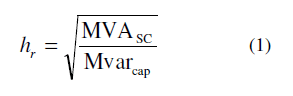
Assuming an ideal constant signal with superimposed noise, the probability distribution can be treated as Gaussian distribution [6] as shown in Fig. 2. In the proposed technique, the measurement of the noise distribution is performed by counting the exceedance of the threshold (Fig. \ref{fig:noise_distribution} – blue lines and dots) for several threshold levels. Measurement can be conducted in two basic concepts: the first one – parallel – assumes an equal number of comparators, each set at different thresholds, the second one – serial – when a single comparator is switching between the threshold levels. There is also possible a combination of these two methods, depending on the system requirements for power, area, and speed.

Fig.2. Noise and its probability distribution (red) and threshold level with counted events (blue).

In the next step, the system fits the distribution curve to the collected data. As it was mentioned before, we are assuming the Gaussian distribution of the noise:

.

with 3 unknown variables: the scaling factor N, the mean value µ, and the standard deviation σ. The accuracy of fitting depends on the number of measuring points (at least 3, because of 3 unknown variables), its position on the fitted curve, and the measurement time. The signal value that we are looking for is the mean of the obtained distribution.

Exemplary System Implementation

Regarding the hybrid pixel detector application requirements, limitations, and driven by a desire for implementation of the considered method, the following system was proposed.

The input stage is implemented as a charge-sensitive amplifier (CSA), working in charge integration mode. It means that the amplifier produces voltage steps at the output as the response to the input current pulses from the detector. The flat output signal requirement is important because of the proper noise distribution recording. In the case when the output signal contains a trailing edge, comparators with fixed threshold levels will raise events incorrectly due to the not stationary nature of the signal. The second issue that can occur while the feedback capacitance of CSA is not discharged is the saturation of the amplifier. Each particle that hits the detector is generating some charge that is integrated in the feedback capacitor. If several events will be added, then the voltage on the feedback capacitor will be too high and the amplifier will leave the operation point. To avoid this, the feedback capacitor should be discharged instantly after the measurement is done. Therefore, an additional CSA resetting circuit should be provided.

The next block is a set of comparators that will execute the measurement of the noise distribution. The selection of the number of comparators and their threshold levels depends on the selected measurement technique (parallel, series or mixed methods shortly described earlier) as well as on the desired (and possible to achieve) resolution and expected dynamic range. Chosen comparators should be fast enough to record all, often extremely sharp, transitions of the noise to provide proper distribution reconstruction.

The signal processing chain ends with a bank of counters that will count and store the comparators’ events. The process of fitting the distribution curve can be executed outside the detector chip, for example, in FPGA or PC. An exemplary system schematic is shown in Fig. 3.

Fig.3. Block diagram of exemplary system implementation.
Verification

Because the described method is not yet implemented in a real circuit, we conducted simulations using an ideal model for confirmation of its usefulness. The model, written in Python language, assumes that:

1. the CSA amplifier works in charge integration mode, which means that we will see voltage steps at its out-put,
2. the comparators are ideal with infinite speed and without metastability,
3. there are no pileup events.

The testbench allows permuting through all key parameters: signal amplitude, noise RMS value, measurement time, number of comparators, and threshold level distribution. In the conducted simulations, we focused on determining the influence of the mentioned parameters on the pro-posed method. It is worth pointing out that the noise vector was generated using a real, implemented in CMOS 40 nm process, CSA circuit with resistive feedback using industry-standard simulator. The generated vector was then imported into our model and added to the ideal signal. Thanks to that, our simulations cover the real noise spectrum, possibly to achieve in real circuits.

For a precisely fitted distribution curve, we need to record as many events as possible in each measuring point to provide enough statistical data. Therefore, we want to maximize the measurement time. This need is in contradiction with the other important parameter of hybrid pixel detectors: the count rate. It describes the maximum intensity of events that can be processed without accuracy loss and other un-wanted effects. The count rate is strictly related to the speed and the dead time of the signal processing chain. Low noise detectors operate in a range from 100 to 100k Hz, which al-lows setting the time for collecting statistical data in the range from 10 μs to 1ms. In Fig. 4, we show the effectiveness of the described method as a function of the measurement time, where time is swept in the range from 1 μs to 50 μs. As we can see in the figure, the number of comparators has no big impact on the measurement when considering the ideal comparator model. It will be more important in the real circuit simulations when comparator mismatches will occur.

Fig.4. The standard deviation of the mean of the fitted curve as a function of measurement time. Input signal amplitude = 100 mV, noise RMS = 10 mV, threshold spacing = 2 mV (symmetrical around 100 mV).

One of the limitations of the described technique is the dynamic range. The measurement range is defined as the distance between the lowest and the highest threshold level. The main limitations stem from area requirements and the need to keep the low spacing between the threshold levels. In hybrid pixel detectors, we want to achieve high spatial resolution, so the pixel area should be as small as possible. This limits the number of comparators implemented in a single pixel. The second ingredient, low spacing between the threshold levels, is related to the CSA output signal noise RMS. Thresholds must be distributed close enough to provide enough points for the reconstruction of the distribution curve (Fig. 5a) but if we bring the thresholds closer, then we lose the dynamic range. Interestingly, the dynamic range can be slightly extended by increasing the circuit noise (Fig. 5b).

Fig.5. (a) – choosing the optimal threshold spacing. The red curve can be easily reconstructed in contrast to the yellow, which cannot be successfully reconstructed. (b) – extending the dynamic range by increasing input signal noise, the number of comparators = 8.

One of the most common methods for improving the energy resolution in hybrid pixel detectors is the CR-RC2 filter. The comparison of the SNR parameter of the proposed method with the CR-RC2 ideal model can be found in Fig. 6. Based on the picture, we can conclude that the proposed method achieves better performance for measurement time higher than 1 µs. The followed comparison was conducted with parameters: the CSA output signal amplitude and the signal noise RMS equals 100 mV and 10 mV respectively, and 4 comparators with 10 mV threshold levels spacing.

Fig.6. Proposed method and CR-RC2 filters SNR comparison.
Conclusion

The discussed method offers a new approach for accurate voltage measurement. The method uses the signal noise distribution measured by counting the number of crossings of a set of reference voltage levels. The method theoretically allows increasing the SNR up to 30 times in the considered measurement time range 1 µs – 25 µs, which is up to 30% better than widely used CR-RC2 filters.

The main limitation of this technique, the dynamic range, was discussed. In the context of hybrid pixel detectors, this solution can be considered as a method for increasing energy resolution as the hardware requirements are small enough to fit the circuit in the 50-100 µm pixel pitch. Further work will focus on implementing the circuit in a real circuit and on searching for a solution for increasing the dynamic range.

Acknowledgments. The presented work has been supported by the Ministry of Science and Education, Poland under contract no.0138/DIA/2020/49.

REFERENCES

[1] Anghinolfi, F., et. al., A 1006 Element Hybrid Silicon Pixel Detector With Strobed Binary Output, IEEE Transactions on Nuclear Science, 39(4), pp. 654–661, 1992.
[2] Gatti, E., Manfredi, P. F., Processing the signals from solid-state detectors in elementary-particle physics, La Rivista Del Nuovo Cimento, 9(1), pp. 1–146, 1986.
[3] Rivetti, A., CMOS: Front-end electronics for radiation sensors, CRC Press, 2015.
[4] White, M. H., et. al., Characterization of Surface Channel CCD Image Arrays at Low Light Levels, IEEE Journal of Solid-State Circuits, 9(1), pp. 1–12, 1974.
[5] Ballabriga, R., et. al., Review of hybrid pixel detector readout ASICs for spectroscopic X-ray imaging, Journal of Instrumentation, Vol. 11, Issue 1, 2016.
[6] S. O. Rice, Mathematical analysis of random noise, The Bell System Technical Journal, Vol. 24, No. 1, pp. 46-156, 1945.


Source & Publisher Item Identifier: PRZEGLĄD ELEKTROTECHNICZNY, ISSN 0033-2097, R. 97 NR 10/2021. doi:10.15199/48.2021.10.34

Harmonics From Solar PV Inverters

Published by Muhammad Najmi Bohari, P.Eng, powerquality.sg THE ABCS OF POWER QUALITY IN SINGAPORE, October 14, 2023.


In general, current harmonics contribution from solar PV inverters do not pose much of a power quality problem. Its ITHD is usually small and negligible as compared to a harmonics-producing load such as a variable speed drive (ITHD for a typical 6-pulse drive ranges between 30% – 50%).

Typically, one will find a Current Total Harmonic Distortion of 3% stated in the datasheet for a quality-brand inverter, as seen here.

.

In Singapore, for a Grid-Tied Solar PV connection, the Licensed Electrical Worker (LEW) (i.e Qualified Person) will have to submit the inverter’s PQ-related type test report to the Grid operator (SP Group). Below is one such example – here it shows the portion whereby the inverter was tested as part of the UK Engineering Recommendation G99 test requirements. Values stated for quality-brand inverters will have its harmonic current emission values well within the limits.

.

You may wonder – One inverter is ok but how about a number of them accumulatively? I had the opportunity to measure numerous sites whereby the rated PV output was accumulatively more than 1MWac.

Here are two sites whereby the background harmonics can be considered to be on the low side and as such the effects of the on-site inverters were more representative (limited ‘contributions’ from the localized electrical network).

All measurements were done using an IEC 61000-4-30 Class A certified Power Quality instruments.

The Current Harmonic Distortion (ITHD) in the trends below have been scaled to the respective aggregated inverters’ rated current (in other words, shown here as Total Demand Distortion (TDD) values).

As observed here, the TDD values were less than 3% and the sinusoidal shape of the current waveforms were very much still visible.

Note: IEEE 519 recommends TDD values of 5% for power generation facilities.

Site #1:

Premises Type: Warehousing / logistics
PV Size: 1352.8 kWp
Aggregated Inverter(s) Rated Current = 1613A @ 400V.
Measurement Point: 2500A PV-AC DB, directly connected to the Premises 5000A Main Switchboard (served by a 3MVA transformer) via 3000A flexible CTs (clamped on 3 sets of 500sqmm cables per phase).
CT direction towards MSB as Load, PV as Source.
VTHD: 0.89% – 3.96% (CP95: 3.6%).

.
.

Site #2:

Premises Type: Solar Farm (On-site loads: Auxiliary power and lighting loads only)
PV Size: 2652kWp (for CS1)
Aggregated Inverter(s) Rated Current = 62A @ 22kV (for CS1).
Solar inverters connected at 400V, stepped-up to 22kV via a 2.5MVA transformer.
Measurement Point: 22kV Incomer 1 from PowerGrid (CS1) via VT and CT.
Note: Solar Farm has 2 x 22kV intakes from PowerGrid – only one intake shown here.
CT direction towards PV as Load.
Solar Farm was connected to a Lightly-loaded 22kV distribution network.
VTHD: 0.59% – 1.22% (CP95: 1.09%).

.
.

Source URL: http://powerquality.sg/wordpress/?p=760

Power Quality Issues and It’s Mitigation Techniques

Published by Tejashree G. More, Pooja R. Asabe,Prof. Sandeep Chawda, (Department of Electrical Engineering, Bhivarabai Sawant Institude Of Technology and Research(w), Wagholi, Pune, India)


ABSTRACT In this paper the main power quality (PQ) problems are presented with there associated causes and consequences. The economic impact associated with PQ are characterized. Also this paper tries to give the solution for reducing the losses produced because of harmonics and increasing the quality of power at consumers’ side.

Keywords: Flywheel, Harmonics, Power Quality, Power Quality Cost, Supercapacitors.

I. INTRODUCTION

Nowadays, reliability and quality of electric power is one of the most discuss topics in power industry. There are numerous types of Quality issues and problems and each of them might have varying and diverse causes. The types of Power Quality problems that a customer may encounter classified depending on how the voltage waveform is being distorted. There are transients, short duration variations (sags, swells and interruption), long duration variations (sustained interruptions, under voltages, over voltages), voltage imbalance, waveform distortion (dc offset, harmonics, inter harmonics, notching, and noise), voltage fluctuations and power frequency variations. Among them, three Power Quality problems have been identified to be of major concern to the customers are voltage sags, harmonics and transients. This paper is focusing on these major issues.

II. POWER QUALITY

It is often useful to think of power quality as a compatibility problem is the equipment connected to the grid compatible with the events on the grid. Compatibility problems always have at least two solutions i.e., either clean up the power, or make the equipment tougher.

Both electric utilities and end users of electrical power are becoming increasingly concerned about the quality of electric power. Electrical PQ is the degree of any deviation from the nominal values of the voltage magnitude and frequency. PQ may also be defined as the degree to which both the utilization and delivery of electric power affects the performance of electrical equipment. From a customer perspective, a PQ problem is defined as any power problem manifested in voltage, current, or frequency deviations that result in power failure or misoperation of customer of equipment. Fig. 1 describe the demarcation of the various PQ issues defined by IEEE Std. 1159-1995.

Fig.1. Demarcation of the various Power Quality issues defined by IEEE Std. 1159- 1995

III. NECESSITY OF POWER QUALITY AUDIT

a. Newer generation load equipment with microprocessor based controls and power electronic devices are more sensitive to power quality variations.

b. Any user has increase awareness of power quality issues. Such as interruptions, sags and switching transients.

c. Many things are now interconnected in a network. Failure of any component has more consequences.

d. Power quality problem can easily cause losses in the billions of dollars. So entire new industry has grown up to analyse and correct these problems.

e. The increase in emphases on overall power efficiency has resulted in continuous growth of application. Such as high efficiency adjustable speed motor drives capacitor use for power factor correction. These results in increase harmonic level which degrade the Power quality.

IV. POWER QUALITY ANALYSISINFORMATION AND STANDARDS

The quality of electricity has become a strategic issue for electricity companies, the operating, maintenance and management personnel of service sector and industrial sites, as well as for equipment manufacturers, for the following main reasons:

a. The economic necessity for businesses to increase their competitiveness

b. The wide spread use of equipment which is sensitive to voltage disturbance and/or generates disturbance itself

V. POWER QUALITY ISSUES

In an electrical power system, there are various kinds of PQ disturbances. They are classified into categories and their descriptions are important in order to classify measurement results and to describe electromagnetic phenomena, which can cause PQ problems. The categories can be classified below,

a. Short-duration voltage variations
b. Long-duration voltage variations
c. Transients
d. Voltage imbalance
e. Waveform distortion
f. Voltage fluctuation
g. Power frequency variations

The most common types of PQ problems are presented in Table I.

The most demanding processes in the modern digital economy need electrical energy with 99.9999999% availability (9-nines reliability) to function properly. Between 1992 and 1997, EPRI carried out a study in the US to characterize the average duration of disturbances. The result for a typical site, during the 6-year period is presented below.

Fig.2. Typical distribution of PQ disturbances by its duration

Table I – Most common Power Quality problems [ 1], [2]

.
.

It is clear that not all these disturbances cause equipment malfunctioning, but many types of sensitive equipment may be affected. Another study of EPRI was undertaken, between 1993 and 1999, in order to characterize the PQ. This study concluded that 92% of disturbances in PQ were voltage sags with amplitude drops up to 50% and duration below 2 seconds.

5.2 COSTS OF POWER QUALITY PROBLEMS

The costs of PQ problems are highly dependant of several factors, mainly the business area of activity. Other factors, like the sensitivity of the equipment used in the facilities and market conditions, among other, also influence the costs of PQ problems.

A. Power Quality Costs Evaluation

The costs related to a PQ disturbance can be divided in:

1) Direct costs: The costs that can be directly attributable to the disturbance. These costs include the damage in the equipment, loss of production, loss of raw material, salary costs during non-productive period and restart costs. Sometimes, during the nonproductive period some savings are achieved, such as energy savings, which must be subtracted to the costs. Some disturbances do not imply production stoppage, but may have other costs associated, such as reduction of equipment efficiency and reduction of equipment lifetime.

2) Indirect cost: These costs are very hard to evaluate. Due to some disturbances and nonproductive periods, one company may not be able to accomplish the deadlines for some deliveries and loose future orders. Investments to prevent power quality problems may be considered an indirect cost.

3) Non-material inconvenience: Some inconveniences due to power disturbance cannot be expressed in money. The only way to account these inconveniences is to establish an amount of money that the consumer is willing to pay to avoid this inconvenience [2], [3].

B. Estimates on Power Quality Costs

Several studies have been made to evaluate the costs of PQ problems for consumers. The assessment of an accurate value is nearly impossible; so all these studies are based on estimates. Some of these studies are presented below

1) Business Week (1991): PQ costs were estimated on 26,000 million USD per year in the United States.

2) EPRI (1994): This study pointed 400,000 million USD per year for PQ costs in the United States.

3) US Department of Energy (1995): PQ costs were estimated on 150,000 million USD per year for United States.

) Fortune Magazine (1998): Stated that PQ costs were around 10,000 million USD per year in United States.

5) E Source (2001): A study comprising continuous process industries, financial services and food processing in the United States, estimated the average annual costs of PQ problems on 60,000 to 80,000 USD per installation.

6) PQ costs in EU (2001): Overall PQ costs in industry and commerce, in European Union, are estimated in 10,000 million EUR per year [6]. The estimates of the various studies differ a lot, but all point to a common factor: the PQ costs are enormous.

C. Costs of Momentary Interruptions

An interruption is the PQ problem with the most perceivable impact on facilities. Table II summarizes the typical costs of momentary interruptions (1 minute) for different types of consumers. The costs presented are without major investments in technologies to achieve ride-through capabilities to cope with the interruption.

Table II – Typical costs of momentary interruptions (1 minute, in $/kW demand, for different types of industrial and services facilities).

.

As it can be seen, the industrial sector is the most affected by interruptions, especially the continuous process industry. In the services sector, communication and information processing is the most affected business area.

The costs of interruptions are also function of its duration. Fig. 3 depicts the costs of interruptions against its duration.

Fig.3. Costs of interruptions as function its duration [3].

5.3 SOLUTIONS OF POWER QUALITY PROBLEMS

The mitigation of PQ problems may take place at different levels: transmission, distribution and the end use equipment. As seen in Fig. 4, several measures can be taken at these levels.

Fig.4. Solutions for digital power [7]
5.3.1 GRID ADEQUECY

Many PQ problems have origin in the transmission or distribution grid. Thus, a proper transmission and distribution grid, with adequate planning and maintenance, is essential to minimize the occurrence of PQ problems.

5.3.2 DISTRIBUTED RESOURCES– ENERGY STORAGE SYSTEM

Interest in the use of distributed energy resources (DER) has increased substantially over the last few years because of their potential to provide increased reliability. These resources include distributed generation and energy storage systems.

Energy storage systems, also known as restoring technologies, are used to provide the electric loads with ride-through capability in poor PQ environment.

Fig.5. Restoring technologies principle [1]

Recent technological advances in power electronics and storage technologies are turning the restoring technologies one of the premium solutions to mitigate PQ problems.

The first energy storage technology used in the field of PQ, yet the most used today, is electrochemical battery. Although some new technologies still rule due to their low price and mature technology.

A. Flywheels

A flywheel is an electromechanical device use to store energy for short durations. During a power disturbance, the kinetic energy stored in the rotor is transformed to DC electric energy by the generator, and the energy is delivered at a constant frequency and voltage through an inverter and a control system. The flywheel provides power during a period between the loss of utility supplied power and either the return of utility power or the start of a back-up power system (i.e.,diesel generator). Flywheels typically provide 1-100 seconds of ride-through time, and back-up generators are able to get online within 5-20 seconds.

B. Supercapacitors

Supercapacitors (also known as ultracapacitors) are DC energy sources and must be interfaced to the electric grid with a static power conditioner, providing energy output at the grid frequency. A supercapacitor provides power during short duration interruptions or voltage sags.

C. SMES

A magnetic field is created by circulating a DC current in a closed coil of superconducting wire. The path of the coil circulating current can be opened with a solid-state switch, which is modulated on and off. Due to the high inductance of the coil, when the switch is off (open), the magnetic coil behaves as a current source and will force current into the power converter which will charge to some voltage level. Proper modulation of the solid-state switch can hold the voltage within the proper operating range of the inverter, which converts the DC voltage into AC power. SMES systems are large and generally used for short durations, such as utility switching events.

D. Comparison of Storage Systems

Fig. 7 shows a comparison of the different storage technology in terms of specific power and specific energy.

Fig.6. Specific power versus specific energy ranges for storage technologies [7].

Fig. 7 shows the specific costs of energy storage devices.

Fig.7. Specific costs of energy storage devices [6].

The high speed flywheel is in about the same cost range as the SMES and supercapacitors and about 5 times more expensive than a low speed flywheel due to its more complicated design and limited power rating. But flywheel can be more cost effective than the battery.

5.3.3 DISTRIBUTED RESOURCES – DISTRIBUTED GENERATION

Distributed Generation (DG) units can be used to provide clean power to critical loads, isolating them from disturbances with origin in the grid. DG units can also be used as backup generators to assure energy supply to critical loads during sustained outages. Additionally DG units can be used for load management purposed to decrease the peak demand.

The most common solution is the combination of electrochemical batteries UPS and a diesel genset. At present, the integration of a flywheel and a diesel genset in a single unit is also becoming a popular solution, offered by many manufacturers.

5.3.4 ENHANCED INTERFACING DEVICES

Besides energy storage systems and DG, some other devices may be used to solve PQ problems. Using proper interface devices, one can isolate the loads from disturbances deriving from the grid.

A. Dynamic Voltage Restorer

A dynamic voltage restorer (DVR) acts like a voltage source connected in series with the load. The working principle of the most common DVRs is similar to Fig. 6. The output voltage of the DVR is kept approximately constant voltage at the load terminals by using a step-up transformer and/or stored energy to inject active and reactive power in the output supply trough a voltage converter.

B. Transient Voltage Surge suppressors (TVSS)

TVSS are used as interface between the power source and sensitive loads, so that the transient voltage is clamped by the TVSS before it reaches the load. TVSSs usually contain a component with a nonlinear resistance (a metal oxide varistor or a zener diode) that limits excessive line voltage and conduct any excess impulse energy to ground.

C. Constant Voltage Transformers (CVT)

CVT were one of the first PQ solutions used to mitigate the effects of voltage sags and transients. To maintain the voltage constant, they use two principles that are normally avoided: resonance and core saturation.

If not properly used, a CVT will originate more PQ problems than the ones mitigated. It can produce transients, harmonics (voltage wave clipped on the top and sides) and it is inefficient (about 80% at full load).

D. Noise Filters

Noise filters are used to avoid unwanted frequency, current or voltage signals (noise) from reaching sensitive equipment. This can be accomplished by using a combination of capacitors and inductances that creates a low impedance path to the fundamental frequency and high impedance to higher frequencies, that is, a low-pass filter. They should be used when noise with frequency in the kHz range is considerable.

E. Isolation Transformers

Isolation transformers are used to isolate sensitive loads from transients and noise deriving from the mains. In some cases isolation transformers keep harmonic currents generated by loads from getting upstream the transformer.

The particularity of isolation transformers is that any noise or transient that come from the source in transmitted through the capacitance between the primary and the shield and on to the ground and does not reach the load.

F. Static VAR Compensators

Static VAR compensators (SVR) use a combination of capacitors and reactors to regulate the voltage quickly. Solid-state switches control the insertion of the capacitors and reactors at the right magnitude to prevent the voltage from fluctuating. The main application of SVR is the voltage regulation in high voltage and the elimination of flicker caused by large loads.

G. Harmonic Filters

Harmonic filters are used to reduce undesirable harmonics. They can be divided in two groups: passive filters and active filters. Passive filters consist in a low impedance path to the frequencies of the harmonics to be attenuated using passive components. Several passive filters connected in parallel may be necessary to eliminate several harmonic components. If the system varies, passive filters may become ineffective and cause resonance.

Active filters analyse the current consumed by the load and create a current that cancel the harmonic current generated by the loads

5.3.5 DEVELOPE CODE AND STANDERDS

Some measures have been taken to regulate the minimum PQ level. One major step in this direction was taken with the CBEMA curve (Fig. 8), created by the Computer and Business Equipment Manufacturer’s Association. This standard specifies the minimum withstanding capability of computer equipment to voltage sags, micro-interruptions and overvoltages.

Fig. 8 – CBEMA curve
Fig. 9 – ITIC curve

This curve, although substituted recently by ITIC (Information Technology Industry Council) curve (Fig. 9), is still a reference in the area of PQ. When the voltage is within the limits determined by the shaded zone, the equipment should function normally. When the voltage is comprised on the zone below the permitted zone, the equipments may malfunction or stop. When the voltage is comprised in the upper prohibited zone, besides equipment malfunction, damage on the equipment may occur.

Other standardization organizations (IEC, CENELEC, IEEE, etc) have developed a set of standards with the same purposes.

5.3.6 MAKE END USE DEVICES LESS SENSITIVE

Adding a capacitor with a larger capacity to power supplies, using cables with larger neutral conductors, derating transformers and adjusting undervoltage relays, are measures that could be taken by manufacturers to reduce the sensitivity of equipment to PQ problems.

VI. CONCLUSION

As conclusion, these Power Quality issues are unwanted phenomenon which are unavoidable but can be reduced using all techniques, but not limited to the techniques that have been discussed. There is no one mitigation technique that will suitable with every application, and whilst the power supply utilities strive to supply improved Power Quality. It means, Power Quality problem cannot be eliminated but we can reduce and try to avoid this problem form occur. The best way to avoid Power Quality problem is by ensuring that all equipment to be installed in the industrial plants are compatible with Power Quality in the power system. This can be achieved by procuring equipment with proper technical specifications that incorporate Power Quality performance of its operating electrical environment.

REFERENCES

[1] J. Delgado, “Gestão da Qualidade Total Aplicada ao Sector do Fornecimento da http://www.ijera.com 177 | P a g e Energia Eléctrica”, Thesis submitted to fulfilment of the requirements for the degree of PhD. in Electrotechnical Engineering, Coimbra, September 2002.
[2] M. Bollen, “Understanding Power Quality Problems– Voltage Sags and Interruptions”, IEEE Press Series on Power Engineering – John Wiley and Sons, Piscataway, USA (2000).
[3] M. McGranaghan, “Costs of Interruptions”, in proceedings of the Power Quality 2002 Conference, Rosemont, Illinois, pp 1-8, October 2002.
[4] D. Chapman, “Costs of Poor Power Quality”, Power Quality Application Guide – Copper Development Association, March 2001.
[5] EPRI, “Creating the Electricity Infrastructure for a Digital Society”, UIE-2000 Conference, Lisbon, 1-3, November 2000.
[6] H. Darrelmann, “Comparison of Alternative Short Time Storage Systems”, Piller, GmbH, Osterode, Germany.
[7] P. Ribeiro, B. Johnson, M. Crow, A. Arsoy, Y. Liu, “Energy Storage Systems for Advanced Power Applications”, Proceedings of the IEEE, vol 89, no. 12, December 2001.


Source & Publisher Item Identifier: Tejashree G. More et al. Int. Journal of Engineering Research and Applications http://www.ijera.com ISSN : 2248-9622, Vol. 4, Issue 4 ( Version 4), April 2014, pp.170-177.

Power Quality in the Portuguese Distribution Network

Published by António LEBRE, Fernando BASTIÃO Nuno MELO, Luísa JORGE Pedro VELOSO, António BLANCO, EDP Distribuição – Portugal. Emails: antoniojose.lebrecardoso@edp.pt, nuno.melo@edp.pt, pedro.veloso@edp.pt, fernando.bastiao@edp.pt, luisa.jorge@edp.pt, antonio.blanco@edp.pt


ABSTRACT There is an increase in the quantity and in the variety of challenges faced by distribution network operators, concerning to Power Quality (PQ). EDP Distribuição, in Portugal, has been developing a comprehensive PQ monitoring program in order to meet all these challenges. This paper presents the state-of-art of the EDP’s PQ monitoring platform as well as the methodology associated to the monitoring program. Some PQ monitoring results for HV/MV and MV/LV substations are also presented, as well as improvement actions in the distribution network and support to the sensitive customers.

INTRODUCTION

EDP Distribuição (EDP D) is a company of the EDP Group Energias de Portugal. In Portugal, EDP D operates approximately 83000 km of High Voltage (HV) and Medium Voltage (MV) lines and cables, 400 HV/MV and MV/MV substations and 62000 transformers used to step down voltage to Low Voltage (LV) users, with a total power capacity around 18700 MVA (figures referred to the end of 2009), being the size of the LV distribution grid around 136000 km. By the end of 2009, EDP D had about 6,1 million of distribution network customers.

Due to extensive rural areas in the country, approximately 80% of HV and MV network is overhead type. This creates severe constraints on the Quality of Service (QoS) in periods of adverse weather conditions, especially during storms and their subsequent consequences.

As an operator of the Portuguese distribution network, fully committed to providing a high level of QoS, EDP D has been systematically monitoring its grids, in particular those of MV and LV levels, since 2001.

The associated PQ monitoring campaigns have been done according to the NP EN 50160 recommended standards and also according to a national QoS Regulation Code, which sets the different indicators and the correspondent minimum quality levels the Distribution Operator must guarantee to all its customers in the different voltage levels.

EDP’S PQ MONITORING PROGRAM

EDP D has been developing a comprehensive PQ monitoring program in order to meet all the actual challenges. This program allows to characterize the PQ in the distribution network and at the customers’ entrance, and improve the operation and maintenance of the distribution network, support customers and report PQ to regulators.

PQ Monitoring Platform and Methodology

To achieve the goal of providing data required to perform all the analysis, a methodology has been implemented, comprising the installation of PQ recorders, communication infrastructures (collecting data), storage systems and analysis software. The basic topology of the PQ monitoring platform is shown in the Figure 1.

Figure 1. EDP’s PQ monitoring platform.

The program is mainly based on 3 months PQ monitoring campaigns in HV/MV and MV/LV substations. These campaigns are performed to assure the requirements of the Portuguese QoS Regulation Code. Recently, EDP D has adopted a strategy of PQ continuous monitoring in all new HV/MV substations. In addition, PQ monitoring at some complaining customers is also carried out.

Systematic Monitoring Campaigns in Substations

Voltage measurements are performed in MV busbars of HV/MV substations, using about 26 portable PQ recorders per quarter. For MV/LV secondary substations there are performed measurements of voltage and current in about 42 LV busbars, per quarter, also with portable PQ recorders.

Continuous Monitoring in HV/MV Substations

According to the EDP D’ strategy to improve the PQ, since 2007 fixed PQ recorders with DFR features have been installed in all new HV/MV substations and in those submitted to a major refurbishment. So far, devices from Siemens (Simeas R) and Qualitrol (BEN 6000), with remote communications by Ethernet, modem and serial port, have been installed. Currently, the new acquisitions are only class A devices according to the IEC 61000-4-30 standard.

Customers Monitoring

Some customers are supported by point PQ monitoring in order to perform an accurate characterization of the PQ supplied and help identify improvement actions. Examples of these customers are sensitive industries and LV microgenerators. Typically, a portable class A PQ recorder is installed for monitoring during a month.

PQ Data Collection and Processing

For systematic monitoring campaigns in substations and customers monitoring, data are collected locally every month, and inserted in an SQL database. For continuous monitoring, the data are collected and stored automatically in the SQL database by scheduled actions.

After each quarter, PQ data of the systematic campaigns are processed in order to issue PQ overview reports to the Portuguese regulator. These reports are performed using a dedicated web based application (QWebReport). All PQ data are also submitted to analysis in order to support operation and maintenance.

PQ MONITORING RESULTS

PQ monitoring results from the HV/MV and MV/LV substations analyzed in the systematic campaigns during the quadriennium 2006-2009 are briefly presented.

HV/MV Substations

During the quadriennium, all the HV/MV substations were analyzed. In the Table 1 are presented PQ results (continuous phenomena) from the 539 MV busbars, in a total of 5819 monitoring weeks. These results are about the percentage of weeks in accordance to the NP EN 50160.

Table 1.

.

The most part of flicker severity “not in accordance”, both in HV/MV and MV/LV substations, is associated to the occurrence of voltage dips.

Figure 2. Voltage dips overview – Cumulative frequency.

In the Figure 2 is shown an overview of the voltage dips recorded in the same MV busbars. The voltage dips characterization was performed as defined in the Annex IV of the Portuguese QoS Regulation Code.

MV/LV Substations

During the quadriennium, at least 2 MV/LV substations per municipality were analyzed. In the Table 2 are presented PQ results (continuous phenomena) from the 580 LV busbars, in a total of 5792 monitoring weeks. These results are about the percentage of weeks in accordance to the NP EN 50160.

Table 2.

.
IMPROVEMENT ACTIONS

Distribution Network

Voltage Variations The main PQ parameter “not in accordance” was voltage variations monitored at LV busbar of MV/LV substations. For the most part, there are situations associated to slight exceeded 110% of nominal value, in a short time. In some cases, situations were identified with origin in voltage regulation in upstream HV/MV substation or proximity of MV distributed generation.

Figure 3. rms voltage values, before and after to decrease one point from tap changers.

Finally, some changes were performed on MV/LV transformer tap changers. For the case study presented in Figure 3, one notices that there were some recorded values slightly above the standard threshold.

After network analysis, the strategy to correct the rms voltage values was to decrease one point from tap changers, as shown in the same Figure. In sequence of the analysis, in some neighbouring MV/LV transformers the same change was made.

Flicker

The second case study is about the voltage flicker recorded in two MV busbars of a HV/MV substation. The substation topology is characterized by two transformers, one busbar for each transformer.

As shown in the Figure 4, the values of voltage flicker in busbar #2 significantly exceeded the limits defined in NP EN 50160.

Figure 4. Voltage flicker (Plt) in busbars #1 and #2 (worst week) and the permissible limit.

In MV busbar #2 some customers were identified as potentially PQ polluters, including foundry (arc furnace), metal processing, recycling of scrap and stone industries.

The flicker level decreases with the increasing network short-circuit power. Therefore, a strategy to mitigate the voltage flicker, immediately and without any investment, was changing the busbar topology, namely, connecting the MV busbars. However, the advantages and disadvantages of this reconfiguration have been carefully studied.

This way we achieved an increase of 58% in short-circuit power in both MV busbars and approximately 16% in a foundry industry.

An additional monitoring in the HV/MV substation validated the procedures in order to mitigate voltage flicker throughout network, to regulatory values.

Harmonics

As a result of these systematic campaigns, EDP D has identified some problems in the distribution network, which deserve careful attention, namely those related to the 5th voltage harmonics levels at particular points along the MV and LV grids.

Resonance Harmonic:

The resonant harmonic hr, based on fundamental frequency impedances, is defined as follows [1]:

.

where hr = resonance harmonic
MVASC = system short-circuit MVA
Mvarcap = Mvar rating of capacitor bank

The resonant harmonic for the MV busbars of all HV/MV substations is calculated from the equation (1).

When the resonant harmonic is approximately close to the 5th harmonic voltage, studies are developed to prevent high voltage distortion based on the identification of potential resonance conditions in most probable network configurations.

In order to deal with the identified problems, to understand their main causes and, as much as possible, to foresee their solution, EDP D has been developing harmonic power-flow analysis models as well as harmonic state estimation models. These have been integrated into DPlan, an analysis and optimization program which evaluates and foresees future trends on harmonics phenomena in the grid, as well as their impact in PQ [2].

Once the non-linear loads have been estimated and the network has been characterized (for the selected frequencies), it is possible to simulate the harmonic behaviour of the system under topology and parameters changes. For example, it is possible to simulate the effect of switching-on capacitor banks, changing tap positions of transformers, connecting busbars and/or reconfiguring the HV or the MV network.

In a case study, the filter function “Harmonic voltage distortion” from a MV network was applied. It was concluded that the increase in the 5th harmonic in MV busbar #1 happens when the capacitor bank (CB) 1, connected to busbar #1, is switched on and the CB 2, connected to busbar #2, is switched off, coinciding still higher values of 5th harmonic with the periods in which the load is lower (off-peak hours). For another busbar, the conclusion is similar.

Figure 5. Harmonic voltage results in MV busbar #1.

The impedance curve depicted in the Figure 5 shows the resonance behaviour for the 5th harmonic.

The harmonic distortion problem was being caused by resonance created by the substation capacitor banks in the MV busbar. This resonance was magnifying the 5th harmonic component in the currents from all the customers on this system, causing high voltage distortion levels.

Optimizing the schedule of both CB, also associated to the management of reactive power in the network, reduces the 5th harmonic voltage to regulatory values.

Events

EDP D has been working on the reduction of the fault incidence on overhead networks in order to decrease the number and duration of voltage dips and short interruptions. Therefore, some actions have been considered, like preventive and predictive maintenance strategies, adjustment of the insulation level to the specific local conditions of the network and implementation of new overhead technologies, such as covered conductors. At the operation level, some actions have been also considered, like optimization of the protection systems, supply of sensitive customers by shorter circuits, from busbars with lower fault incidence or higher voltage levels, and increasing HV network robustness.

Sensitive Customers

Potentially sensitive customers are invited by EDP D to report PQ disturbances during the systematic monitoring campaigns. Mostly, they report production disturbances facing to voltage dips. The sensitivity is variable, but an important number of them are sensitive to voltage dips of short magnitude and/or short duration. Continuous processes supported by PLC, ASD and other electronic devices are very sensitive to voltage dips and long downtime periods can be experienced. There are typical difficulties to adopt immunization solutions and reengineering strategies to improve the process reliability at the customer level.

Based on the available information, root causes and effects of reported disturbances are analyzed. This allows to check the sensitivity of customers, as well as to launch the research for improving actions at distribution network and customers levels.

With the technical support of EDP D, the following improvement actions are some examples of successful cases: immunization of glass production machines; installation of static and dynamic UPS in moulds, dairy and ceramics industries; immunization of fan systems driven by ASD in cement and chemical industries; optimization of the distribution network and immunization of command and control systems in the chemical industry; consultancy in the adoption of several immunization solutions in the automotive components industry; implementation of alternative supplying circuits with fast transfer switches.

MAIN CHALLENGES

In terms of PQ, the challenges are mainly related to the customer sensitivity to voltage dips, increasing penetration of Micro-Generation (MG), trends of regulation to request higher PQ levels, as well as management of large amounts of monitoring devices and PQ data.

Since 2007, there has been a noticeable increase of MG in Portugal, leading to an installed base of around 10000 MG units in the end of 2010. This amounts to around 30 MW of installed MG power. This increasing number of microgenerators injecting power in the LV grid is bound to cause a significant impact on the main grid PQ parameters. EDP D has performed some monitoring studies including a few MG units and the MV/LV substations to which they are attached, relating the results to their location and the types of load they feed. The first conclusions point to non-degradation of the grid operating conditions within the current legal power limitations, in the vicinity of MV/LV substations (~200 meters) but, however, some parameters may change with different conditions. Given the interest they raised, these studies will be continued with monitoring campaigns of larger dimension, in duration, scope and periodicity.

On the other hand, in order to implement continuous PQ monitoring at the distribution network scale, some developments are expected in the solutions available to PQ data transfer, storage and management. An important requirement is the adoption of standards, like PQDIF format, to integrate data from devices provided by several vendors.

CONCLUSIONS

Despite the current challenges, it has been possible to develop a comprehensive PQ monitoring program, including several monitoring weeks in more than one thousand MV and LV busbars. Furthermore, it is expected an increasing of the measuring points with recent developments in the EDP’s PQ Monitoring Platform, namely with the continuous monitoring strategy in HV/MV substations. Based on the PQ monitoring results, EDP D has been adopting several measures aiming to develop its actions in the distribution network, such as, mitigation of harmonic distortion, mainly the 5th harmonic, attenuation of flicker induced by industrial loads, reduction of faults in overhead networks in order to decrease the incidence of voltage dips and short interruptions, as well as adjustment of voltage levels in some LV busbars. The PQ monitoring campaigns are also giving support to sensitive customers who wish to adopt immunization solutions and improve their production reliability.

Power Quality is becoming an important reference factor to distribution network operators concerning its contribution to the global QoS.

Acknowledgments The authors thank the availability and collaboration from the colleagues Teresa Couceiro and Flávio Cação.

REFERENCES

[1] R. Dugan et al., 2003, Electrical Power Systems Quality, McGraw-Hill, USA, 167-224.
[2] C. Santos et al., 2009, “Voltage distortion in largescale MV and HV distribution networks: harmonic analysis and simulation”, 20th International Conference on Electricity Distribution – CIRED.


Source: CIRED 21st International Conference on Electricity Distribution Frankfurt, 6-9 June 2011. Paper No 1021. URL: http://www.cired.net/publications/cired2011/part1/papers/CIRED2011_1021_final.pdf