Published by Alex Roderick, EE Power – Technical Articles: Energy Generation Through Wind Power Systems, August 21, 2021.
Because winds are primarily caused by uneven heating effects of the sun, wind energy is considered to be an indirect form of solar energy and is therefore renewable.
The primary cause of winds is the uneven heating of the earth’s surface by the sun, which depends on latitude, time of day, and the distribution of land and large bodies of water, particularly the oceans. Another cause of winds is fluid friction between the atmosphere and the earth’s surface, which allows the earth to drag the atmosphere around, producing turbulence. Horizontal components of wind velocities are normally much greater than the vertical velocity components.
The kinetic energy of the wind, and therefore the wind’s power-generating potential, is proportional to the cube of wind velocity. Because winds are primarily caused by uneven heating effects of the sun, wind energy is considered to be an indirect form of solar energy and is therefore renewable.
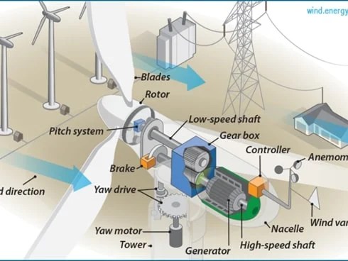
Wind power is the use of airflow through turbines to provide energy to turn electric generators. A small wind turbine is a wind turbine that can be installed on properties as small as one acre in areas with sustained winds to create electricity. Small wind turbines typically have three propeller-like blades around a rotor connected to a shaft that spins a generator (see Figure 1). The two types of wind turbine systems are grid-connected wind turbine systems and off-grid (stand-alone) wind turbine systems.
Figure 1.Small wind turbines can be installed on properties that are one acre or larger. Image courtesy of Energy.gov
Grid-Connected Wind Turbine Systems
Although small wind turbines are typically off-grid systems, they can also be connected to a utility’s electrical distribution system (grid). These are called grid-connected wind turbine systems. To work effectively, a small wind turbine that is connected to the grid requires an average annual wind speed of about 10 mph to 15 mph.
Grid-connected wind turbines are only allowed to operate when the utility grid is online. During power outages, the wind turbine is required to shut down due to safety concerns from islanding. Islanding is a condition in which a generator continues to power a location when electrical grid power is not present. Islanding can be dangerous to utility workers, who may not realize that a circuit is still powered.
A grid-connected wind turbine project requires working with the utility to make the interconnection. Utilities have developed interconnection standards for the equipment and special meters that need to be installed at the service. Also, an electrical inspector must sign off on the system before the utility will allow connection to the grid. The inspector will require that all electrical work be completed by a licensed electrician.
Off-Grid (Stand-Alone) Wind Turbine Systems.
Small wind turbines that are not connected to the grid are called off-grid wind turbine systems, also known as stand-alone wind turbine systems. Off-grid wind systems can be installed to gain energy independence from the utility. However, a homeowner should be comfortable with uncertain power production due to fluctuations in wind speed. Off-grid wind turbine systems can be combined with solar PV systems to create a more reliable hybrid electric system. Wind and solar PV energy generation, along with battery storage, can offer enhanced improvements to an off-grid system.
Off-grid wind turbine systems are typically smaller and less expensive than grid-connected systems. Small wind turbines that are off-grid systems require annual maintenance. Annual maintenance usually requires that a person climb up the wind turbine tower. However, small wind turbines with tilt towers can be lowered to the ground for maintenance.
The kinetic energy of the wind is converted to electrical energy using a wind turbine. There are primarily two types of wind turbines, each being characterized by the orientation of the axis or shaft.
A horizontal axis wind turbine (HAWT) typically consists of a set of three blades mounted to a horizontal shaft that is connected to an electrical generator. This traditional “windmill”-style turbine is used in a variety of applications, from 5-MW wind farms to 100-kW residential applications.
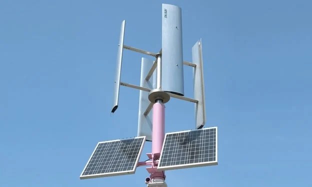
A vertical axis wind turbine (VAWT) resembles an “eggbeater” and typically consists of three blades mounted to a vertical shaft. VAWTs are primarily used in small-scale applications and are less common than HAWTs. A vertical axis wind turbine is a design of small wind turbine that does not require exact wind orientation and can still operate in unfavorable wind conditions. Unlike a traditional wind turbine on a horizontal axis, a vertical axis wind turbine does not have to track the wind to produce electricity. Some vertical axis wind turbines can also have solar panels embedded in their housings, which increases the energy output while using the same square footage of space (see Figure 2).
Figure 2. A vertical axis wind turbine does not require exact wind orientation and can operate in unfavorable wind conditions. Some units have solar panels embedded on top of their housing.
Purchasing Wind Energy Systems
To purchase a wind energy system, it is important to know the necessary tower height, the power required from the turbine, the installation cost, and the cost to maintain the system. There may be grants or incentives available to defer some costs. A homeowner should also purchase wind insurance for liability and damage to equipment.
The average height of a small wind turbine is about 80′, which is about twice the height of a residential telephone pole. However, small wind turbines can range in height from 30′ to 140′. The output needed to power a dwelling can range from 2 kW to 10 kW. A large, grid-connected system can range from $10,000 to $70,000, while the purchase and installation of an off-grid small wind turbine (less than 1 kW) generally cost $4,000 to $9,000. The ROI for a small wind turbine ranges from 6 years to 30 years. The ROI is based on the energy use of the dwelling, average wind speeds, and the turbine’s height above ground.
Less than 1% of all small wind turbines are used in urban applications due to zoning restrictions and poor wind quality in densely built environments. Wind resource information can be found through the National Renewable Energy Laboratory (NREL), local airport wind data, and state guidelines through the DOE’s Office of Energy Efficiency and Renewable Energy. There are incentives for the purchase of wind turbines and for the sale of excess electricity. The Public Utility Regulatory Policies Act of 1978 (PURPA) is a federal regulation that requires utilities to connect with and purchase power from small wind energy systems.
Author: Alex earned a master’s degree in electrical engineering with major emphasis in Power Systems from California State University, Sacramento, USA, with distinction. He is a seasoned Power Systems expert specializing in system protection, wide-area monitoring, and system stability. Currently, he is working as a Senior Electrical Engineer at a leading power transmission company.
Published by Alla Eddine TOUBAL MAAMAR, M’hamed HELAIMI, Rachid TALEB, Electrical Engineering Department, Hassiba Benbouali University, LGEER Laboratory, Chlef, Algeria
Abstract. In this study, the analysis, simulation and realization of direct current to alternating current multilevel inverter are discussed. Inverter operation with the high-frequency mode is evaluated and tested for the validation of the topology. This inverter type will be used in an induction heating system or other industrial applications need high-frequency, periodic and alternating signals. The control signals of electronic switches are implemented via an open-source board, Arduino, composed of an Atmega2560 microcontroller. Simulation with MATLAB/Simulink environments and experimental results are presented, comparatively, for a comparison.
Streszczenie. W artykule zaprezentowano symulację, analizę I eksperymentalną weryfikację przekształtnika. DC/AC. Ten typ przekształtnika może być zastosowany w nagrzewaniu elektrycznym lub innych zastosowaniach wymagających prądu wcz. Analiza, symulacja I eksperymentalna weryfikacja wielopoziomowego przekształtnika DC/AC wysokiej częstotliwości..
Keywords: Power Electronic, Multilevel Inverter, High-frequency Signals, MATLAB/Simulink Słowa kluczowe: przekształtnik DC/AC, przekształtnik wysokoczęstotliwościowy.
Introduction
A most of renewable energies source like solar energy produce direct current, the Direct current (DC) must be converted into an alternating current (AC), because most of the devices used in our daily lives use it, the circuit which converts DC power into desired output voltage, frequency, and AC power form is called as Inverter [1]. If several DC voltage sources are used as an input or special topology of an inverter is implemented, a desired output voltage stages can be obtained, the inverter will be named multilevel inverter. There are many research and proposed topologies of the conventional multilevel inverter [2], [3], capacitor clamped inverter [4], diode clamped inverter [5] and the cascaded multilevel inverter is the most popular inverter, is used for many applications [6].
The main aims of this research are to analysis and simulation of High-Frequency DC/AC hybrid Five-level Inverter properties with MATLAB/Simulink, this type of converter is widely used in standby power supplies, induction heating, and induction motor drives [7]. A Realization and test of the presented topology are important steps for validation of obtained results.
The paper is organized as follows: In the second Section, The analysis of the hybrid topology of Five-level inverter operation have been discussed, the simulation and realization results are presented in the later sections. Eventually, conclusions are given.
Analysis of the DC/AC Multilevel Inverter Operation
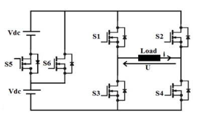
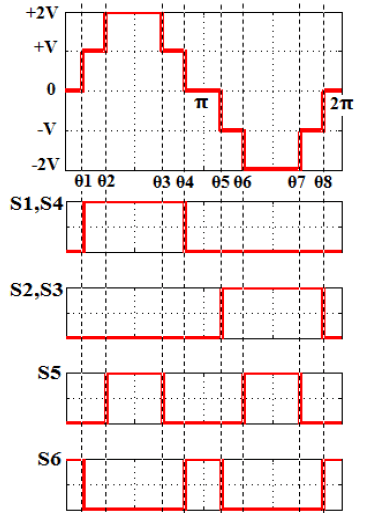
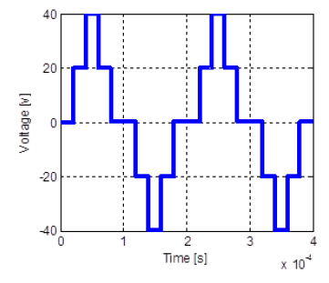
Fig. 1, showing the topology of a five-level inverter [8], this topology consists of less number of switches when to be compared with the conventional topology of a five-level cascaded H-bridge inverter. The presented topology consists of two separate DC sources and six semiconductor devices switches. By switching the semiconductor devices at the appropriate firing angles, we can obtain the full cycle of the phase voltage shown in Fig.2.
Inverter topology is composed of H-bridge inverter with two switching cells (S1, S3 and S2, S4) and two extra switches (S5, S6), depending on the states of the electronic switches, five operating sequences can be distinguished during a switching period T.
Sequence 1: (U = 0), the switch S6 is closed and switches S1, S2, S3, S4, S5 are opened. Sequence 2: (U= +V), the switches S1, S4 are closed and switches S2, S3, S5, S6 are opened.
Fig.1. the structure of the five-level inverter
Fig.2. the full cycle of the phase voltage of 5-level inverter
Sequence 3: (U= +2V), the switches S1, S4, S5 are closed and switches S2, S3, S6 are opened. Sequence 4: (U= -V), the switches S2, S3 are closed and switches S1, S4, S5, S6 are opened. Sequence 5: (U= -2V), the switches S2, S3, S5 are closed and switches S1, S4, S6 are opened.
Simulation of a Five-level Inverter
Simulation of the five-level inverter is done in MATLAB environment (SIM/POWER/SYSTEMS). The simulated circuit is a MOSFET based resistor Load, R=10 ohm.
Fig.3. Simulation model of 5-level inverter
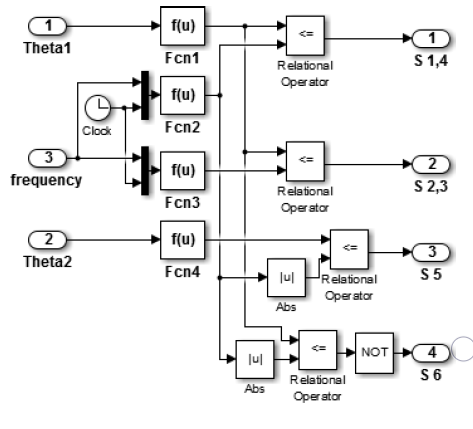
Fig.4. Model of switches control
The functions of the switches control are determined by the following relationships.
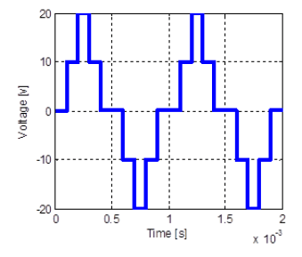
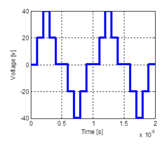
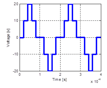
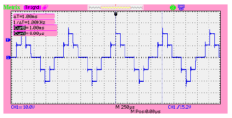
“Fig. 5”, “Fig. 6”, “Fig. 7”, “Fig. 8”, shows the output voltages of resistor load using MATLAB/Simulink with different frequency, 1 [KHz], 5 [KHz], and dc =10 [v], dc =20 [v].
Fig.5. Voltage waveform, with f=1 [Khz] and dc =10 [v]
Fig.6. Voltage waveform, with f=1 [Khz] and dc =20 [v]
Fig.7. Voltage waveform, with f=5 [Khz] and dc =10 [v]
Fig.8. Voltage waveform, with f=5 [Khz] and dc =20 [v]
Arduino ATmega2560 Microcontroller and Digital PWM signals generations
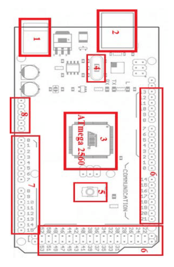
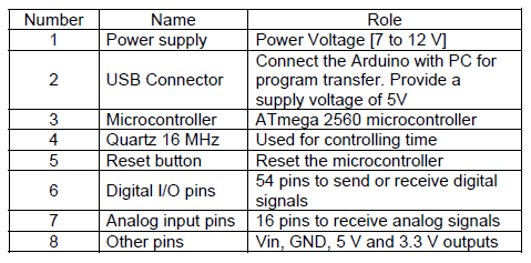
Arduino is a printed circuit, consisting of several electronic components and a microcontroller to receive, analyze and produce electrical signals, the main advantage of the Arduino technology is an open-source platform and you can directly load the programs into the device without the need of a hardware programmer to burn the program. Arduino board based on an ATmega2560 microcontroller is shown in the Fig.9. It consists of 54 pins, Where 14 digital inputs/outputs pins and 6 analogue inputs/outputs pins, a 16MHz clock, has 256 KB of flash memory, 8 KB of RAM and 4 KB of EEPROM [9], [10].
In several applications, which are powered by inverters, it is necessary to control the output voltage, PWM as one of the most efficient techniques to vary the voltage gain. Modern microcontrollers (PIC Microcontroller, ARM Cortex M, PIC, ARDUINO UNO card, ARDUINO ATmega2560 card, …etc.) all have peripherals or pins dedicated specifically to PWM generation. The method of this work has programmed the TIMER of the ARDUINO ATmega2560 card to transform it into a digital PWM generator, the principle is to create a digital configured signal of frequency and duty cycle. A timer is a register located in the microcontroller that is incremented or decremented each time it receives a pulse from a clock signal. Therefore, a timer is a counter, capable of counting the time that elapses, hence its name counter timer.
Fig.9. Components of the Arduino ATmega2560 board.
The ATmega 2560 microcontroller has one 8-bit counter timer numbered 0 and four 16-bit counter timers numbered 1, 3, 4 and 5. The Timer configured with two control registers TCCRnA and TCCRnB. The clock used is the main clock of the Arduino ATmega 2560, which has a frequency of 16 MHz. The selection of the clock mode operation is made on bits 2, 1 and 0 of the TCCRnB register. To produce the waveform signal, it is necessary to use the Timer in a wave generator mode. The main generator modes are Normal Mode, Fast PWM Mode, and Phase Correct PWM Mode. The selection is made with the 4 bits: WGMn0, WGMn1, WGMn2 and WGMn3 (Waveform Generation Mode), the first two are bits 0 and 1 of the TCCRnA register; the last two are bits 2 and 3 of the TCCRnB register. The counter also includes OCRnX register (Output Compare Register) which is compared to the TCNT register to trigger various actions. This counter used to configure the duty cycle of the PWM signals[9], [11].
Table 1. Name and Role of Arduino components
.
Realization of a Five-level Inverter
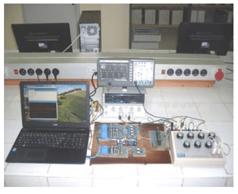
Fig. 10, Shows the experimental prototype of the five-level inverter, consists of six MOSFET switches IRF 640 controlled by driver circuits with TLP 250 optocoupler, two power supplies (Vdc). The control signals have been implemented using Arduino ATmega2560 Microcontroller and PC with open source software (Arduino IDE).
Fig.10. A Laboratory prototype of a Five-level inverter
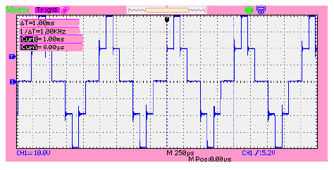
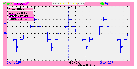
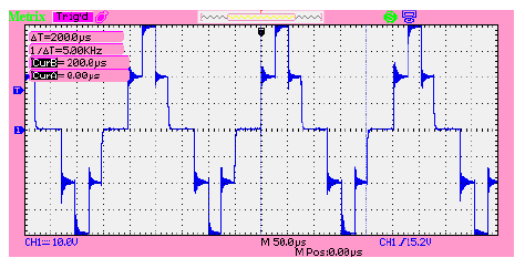
“Fig. 11”, “Fig. 12”, “Fig. 13”, “Fig. 14”, shows the experimental phase voltage of the five-level inverter with different frequency, 1 [KHz], 5 [KHz], and power voltages, 10 [v], 20 [v].
Fig.11. Experimental phase voltage with f=1 [KHz] and dc=10 [v].
Fig.12. Experimental phase voltage with f=1 [KHz] and dc=20 [v].
Fig.13. Experimental phase voltage with f=5 [KHz] and dc=10 [v].
Fig.14. Experimental phase voltage with f=5 [KHz] and dc=20 [v].
The simulation results of the 5-level output voltage are presented in “Fig. 5”, “Fig. 6”, “Fig. 7”, “Fig. 8”, and experimentally validated, the experimental prototype and results of the output voltage waveforms generated by inverter are presented in “Fig. 11”, “Fig. 12”, “Fig. 13”, “Fig.14”, There are a small shifts between the two form of results (simulation and realisation), but generally, the obtained results show the good concordance existing between the simulation model and the real system, the small shift because of the electrical perturbations of electronic components. The output power of the five-level inverter can be controlled by adjusting the frequency or the duty cycle of the switches.
Conclusion
The analysis, simulation and realization of a hybrid five-level inverter are discussed in this paper. The effectiveness of the analysis is verified by the obtained results.
The high-frequency DC/AC inverter has been chosen because our future purpose is the study of induction heating, and the frequency is the main physical parameter of this type of converters.
The results obtained are satisfactory because the simulation model of a multilevel inverter with Matlab is validating experimentally using Arduino ATmega2560 microcontroller. This work opens new ways for future research with other topologies, other electronics devices controllers like the pic microcontroller or FPGA and levels of the inverter can be increased.
REFERENCES
[1] Rajkumar M., Manoharan P.S., Modeling and Simulation of Five-level Five-phase Voltage Source Inverter for Photovoltaic Systems, Przeglad Elektrotechniczny, 10 (2013), 237-241 [2] Babaei E., Alilu S., and Laali S., A New General Topology for Cascaded Multilevel Inverters With Reduced Number of Components Based on Developed H-Bridge, IEEE Trans. Ind. Electron., 61(2014), NO. 8, 3932-3939 [3] Gupta K. K., Ranjan A., Bhatnagar P., Sahu L. K., Jain S., Multilevel Inverter Topologies With Reduced Device Count: A Review, IEEE Trans. Power Electron., 31(2016), No. 1,135-151 [4] Raman S. R., Cheng K. W. E., Ye Y., Multi-Input Switched- Capacitor Multilevel Inverter for High-Frequency AC Power Distribution, IEEE Trans. Power Electron., 33(2018), No. 7, 5937-5948 [5] Shi S., Wang X., Zheng S., Zhang Y., Lu D., A New Diode- Clamped Multilevel Inverter With Balance Voltages of DC Capacitors, IEEE Trans. on Energy Conversion, 33 (2018), No.4, 2220-2228 [6] Ebrahimi J., Babaei E., Gharehpetian G. B., A New Topology of Cascaded Multilevel Converters With Reduced Number of Components for High-Voltage Applications, IEEE Trans. Power Electron., 26 (2011), No. 11, 3109-3118 [7] Waradzyn Z., SKAŁA A., ŚWIĄTEK B., KLEMPKA, KIEROŃSKI R., ZVS single-switch inverter for induction heating optimum operation, Przeglad Elektrotechniczny, 2 (2014), 32- 35 [8] El-Naggar K., Abdelhamid T. H.,Selective harmonic elimination of new family of multilevel inverters using genetic algorithms, Energy Conversion and Management, 49 (2008), nr 1, 89–95 [9] Montironi, M.A., Qian, B., Cheng, H.H., Development and application of the ChArduino toolkit for teaching how to program Arduino boards through the C/C++ interpreter Ch, Comput Appl Eng Educ, 25 (2017), 1053– 1065 [10] Arduino.cc, Arduino Mega 2560, Accessed 03/11/2019. Available: https://store.arduino.cc/arduino-mega-2560-rev3 [11] Atmel-Datasheet, 02/2014. Accessed 03/11/2019. Available: http://ww1.microchip.com/downloads/en/DeviceDoc/Atmel-2549-8-bit-AVR-Microcontroller-ATmega640-1280-1281-2560-2561_datasheet.pdf
Published by Yuriy BORODENKO1, Leonids RIBICKIS2, Anatolijs ZABASTA3, Shchasiana ARHUN4, Nadezhda KUNICINA5, Anastasia ZHIRAVETSKA6, Hanna HNATOVA7, Andrii HNATOV8, Antons PATLINS9, Konstantins KUNICINS10, Kharkiv National Automobile and Highway University (1), Riga Technical University (2), Riga Technical University (3), Kharkiv National Automobile and Highway University (4), Riga Technical University (5), Riga Technical University (6), Kharkiv National Automobile and Highway University (7), Kharkiv National Automobile and Highway University (8), Riga Technical University (9), Riga Technical University (10)
Abstract. In this paper is presented a simulation model of the electric drive (ED) system for the diagnosis of an electric vehicle. Model is built by the method of spectral analysis of the electrical process of propulsion systems power supply. Moreover, the efficiency of ED is a key challenge for the research team. The developed model adequately imitates the electrical processes that occur in the power circuits of the ED system with an AC converter-fed motor. The developed model can be used for virtual studies of dynamic ED modes and studies, and optimization tasks.
Streszczenie. Przedstawiono model symulacyjny napędu elektrycznego umożliwiający diagnostykę pojazdów elektrycznych. Model bazuje na analizie widmowej ciągu. Analizowana jest też efektywność napędu. Model mopże także służyć do wirtualnej analizy dynamiki. Diagnostyka systemu napędowego z wykorzystaniem analizy spektralnej.
Keywords: electric car, electric drive, diagnostics, transport model. Słowa kluczowe: pojazd elektryczny, napęd, analiza widmowa.
Introduction
Currently, various types of diagnostic systems are being used increasingly on modern vehicles. For electric vehicles, one of the most important elements is the electric drive (ED), therefore, it should be diagnosed with the greatest attention. Timely detection of ED faults will reduce costs during its operation, maintenance and repair. In this paper, a simulation model of the ED system for the electric vehicle diagnosis by means of the spectral analysis method for the electrical process of propulsion systems power supply is built. Moreover, the efficiency of ED is a key challenge for the research team. The developed model adequately imitates the electrical processes that occur in the power circuits of the ED system with an AC converter-fed motor. The spectral characteristics of the high-voltage battery discharge current function allow a qualitative and quantitative assessment of the starting and power modes of ED, as well as evaluate the efficiency of the solution in general. The composition of the dominant harmonics in the spectrograms depends on the design parameters of the electric motor and the circuit design of the voltage inverter. To increase the informational content of spectrograms, it is advisable to use various FFT analysis formats. The developed model can be used for virtual studies of dynamic ED modes and studies, and optimization tasks related to the identification of structural and parametric faults arising in its circuits.
Environmental issues and the depletion of natural resources have become the main engine for the development of energy-efficient technologies worldwide. This is especially true for the transport industry. The use of alternative sources of electric energy in transport and infrastructure solves these problems partially [1] – [3]. A more tangible result is given the replacement of vehicles with internal combustion engines to cars using electric traction.
The analysis of different transport network exploitation conditions, integration of electric transport in transport network, as well as future development of new power supply solutions within the frame of smart city context are being discussed. [4,5] The developed approach [6] will allow the usage high-performance (HPC) capabilities, which are considered to be the main technology of the next generation of computing. In addition, the development focuses on the graphic processing unit (GPU), where the consumption of energy is several times lower than the classic architecture of computing elements. The proposed data transmission method has been tested on the basis of Interactive Technology, proposed in [7].
The use of electric traction in road transport allows us to solve problems associated with the improvement of its environmental performance and fuel efficiency. Today, two main areas of concept development are considered – the use of hybrid power plants that use an auxiliary electric motor, and the use of all-electric traction from battery power sources [8,9].
One of the aspects of the development of automotive electric drives (ED) is the reduction of operating costs during their operation, maintenance and repair. Such problems are solved at the stages of ED development (adaptation of the design, integration of diagnostic systems) and during the transport process (use of monitoring systems for technical condition) [8, 9].
The information basis of these systems is knowledge and data base for expert analysis [10]–[14]. For this reason, the article discusses a method for the quantitative assessment of electrical processes occurring in the ED power supply circuit for the purpose of using the received information as a diagnostic one.
The ED electric structure consists of the information part (sensors and controllers of the control system) and the power electric part (voltage converters, electric machines).
Applied integrated self-diagnosis systems allow the monitoring of technical condition of the control system components directly connected to the electronic control unit, but do not allow the identification of malfunctions of actuation devices of the power part, which are remotely controlled [14] – [15]. Thus, [20] proposes the use of the built-in processor and bidirectional communication with an intelligent actuation device in the steering system. This enables self-diagnosis, which should lead to increased reliability.
Testing of the ED power electric [19] part traditionally begins with monitoring the voltage levels of all power sources at idle and under rated load in static modes. Next, the ED operation is checked in dynamic modes [21].
When using the AC converter-fed motor with a primary DC source and a voltage inverter, the information about the level (average value) of voltage or current is not enough to identify a malfunction.
In [15], a qualitative analysis of the processes in the AC converter-fed motor system at stationary modes without a secondary power source (overvoltage converter) was made. The system model used a simplified model of a high-voltage battery (HVB) in the form of an idealized EMF source with internal resistance.
The aim of the work is to build an electric drive system simulation model for diagnosis of an electric vehicle by the spectral analysis method for the electrical process of propulsion systems power supply.
Simulation model of an electric drive system
The power part of the car’s electric drive system consists of an overvoltage converter, an inverter and a synchronous electric motor with rotor position sensors [15]. To increase the supply voltage in the converter circuit, a reactor (inductance) is used in which self-induction EMF pulses arise as a result of switching the current of the power circuit (Fig. 1) [15].
Fig.1. Electric drive circuit with AC converter-fed motor
The electric motor of the drive is a ED (AC converter-fed motor) with excitation from permanent magnets and perceives the position of the accelerator pedal AP (α) and the feedback signal of the angular position of the shaft of the machine MS (ω) for control actions. The controller of the electric machine generates the control pulses of the keys of the converter of increased DC voltage (L, VT, VD1, C2, R) and the inverter UI.
The period of the working cycle of electrical processes in the converter circuit is determined by the switching time of the current in the reactor L with a transistor switch VT. During the closed state of the key, the voltage of the nickel-cadmium HVB UB = 250 V is applied to the reactor under the action of which a current arises in the circuit, which increases with time to a steady state. During the opening of the key (switch), the reactor induces EMF pulses.
The amplitude of the pulses generated as a result of transient processes exceeds the level of HVB voltage supplied to the reactor. At the output of the converter circuit, an integrating capacitor C2 is included, which maintains a constant voltage at the level of amplitude values of 500 V. The diode VD1 eliminates the discharge of the capacitor C2 through a transistor switch, during its open state. The diode VD2 protects the transistor switch VT from surge impulses. Buffer capacitor C1 smooths out the surges in the supply circuit during transients.
To conduct virtual research, a simulation model of the ED system was built in the application package Matlab / Simulink. The model of an electric drive system consists of a primary voltage source Battery, a ED system of AC converter-fed motor [22] and an overvoltage converter (secondary power supply) (Fig. 2).
Unlike previous studies [16, 17] of the model, a circuit with an increased DC voltage converter is considered and a HVB model is used, taking into account its energy and conditional Faraday capacities. A NiMH-type HVB model (Battery) with a rated voltage of UB = 220 V and a rated capacity of SB = 5 A / h was selected as the primary voltage source. The reactor L is parameterized with an inductance L = 0.5 mH and an active resistance of the winding r = 0.01 Ohms. The Generator block (rectangular pulse generator) imitates the IGBT key control signal, which in a real system comes from the controller of an electric machine. An increased voltage of 500 V from the converter is supplied to the IGBT Inverter in which the phase currents of the “Ventil Dvig” AC converter-fed motor are switched. Maintaining a given speed of rotation of the electric motor under load (block 850) is carried out through a comparison circuit “Speed Ref” of the current speed of rotation of the motor shaft with its given value.
Fig.2. Scheme of a simulation model of an electric drive system with a AC converter-fed motor
In the model diagram, model No. 12 of a AC converter-fed motor is used, which develops a rated torque MN = 35 Nm at a rated rotation speed of nN = 3000 min-1. The circuit model of the electric drive system is investigated in a stationary mode. The signal of the generator (Generator) is: frequency 20 kHz, amplitude 3 V, duty cycle 50%. The motor load is 37 Nm, the shaft rotation speed n = 850 min-1 is supported. The load on the motor occurs after 0.3 s. after its inclusion (the function is implemented by the “Navantagenna” unit). The data of the passive elements of the voltage converter model correspond to the values of the parameters of the circuit elements of the Lexus RX400h vehicle voltage converter block.
Electrical processes simulation results
According to preliminary studies, the harmonic composition of the current function in the IB power supply circuit is the best diagnostic parameter from the point of view of information content, sensitivity and manufacturability. The results of the study of the model are shown in Fig. 3 [15].
When starting the engine after turning on the power 0 <t <0.05 s, the torque M, which overcomes the friction forces, and the inertia of the rotor mass and current iB, have maximum values. A noticeable surge in current consumption is caused by a charge on the capacitor C1. The maximum value of this current IB = 450 A is limited only by the internal resistance of the power source r0, and the duration of the surge is limited by the value of the capacitor C1.
Further, over a period of 0.05 <t <0.1 s, the torque gradually decreases as the engine rotor accelerates. The rotor speed n, in this case, increases to constant idle speed. The temporal functions of these mechanical quantities have a similar oscillatory character, damping in time. With a fixed electric motor power, these periodic functions are phase shifted by half a period, and the product of their instantaneous values is equal to the mechanical power on the shaft.
Fig.3. Functions of the output characteristics of the electric drive: a – torque on the motor shaft; b – rotor speed; c – current in the HVB circuit
After starting and accelerating an unloaded engine, during a period of 0.1 <t <0.3 s, in idle mode, the torque M is almost zero, the rotor speed is kept constant at a given level (n = 850 min-1), and the battery discharge current IB has minimum values of the order of units of amperes.
Fig.4. Spectral characteristics of the current functions in the HVB circuit in the AC converter-fed motor modes: a – start without load; b – start-up under load; c – idling; d – stationary load
After the load is applied to the motor shaft at t> 0.3 s, the angular velocity of the rotor shaft has a slight fluctuation with the frequency of change of instantaneous torque values, the actual value of which is determined by the resistance moment (given load). In the steady state under load, periodic processes occur due to the switching of the transistor switches of the inverter (with a frequency of multiple rotational speeds of the rotor of the electric motor) and the voltage converter (with a generator frequency of 20 kHz).
The analysis of spectrograms Spectral
FFT analysis (fast Fourier transform method) was carried out for certain modes of electric drive [18] (sections of the function IB). In this case, the sensitivity of the diagnostic parameter is determined by the discrepancy between the amplitudes and phase shifts of the individual harmonics of the spectrum for a given mode of the drive system, and the information content is determined by the discrepancy of the spectrograms of the selected mode for various technical conditions (operational and faulty).
The results of previous studies, on this occasion, show that for each mode of operation and the technical condition of the electric drive, certain spectrogram formats should be selected. To do this, select the “FFT Analysis” mode in the “Powergui” instrument menu and configure the spectrum analyzer options (maximum observation frequency “Max Freqency” and the base frequency of the relative harmonic amplitude reference (Fundamental Frequency FF). The results of the expansion of the functions in Fourier series are shown in Fig. 4 [22].
The figures show the amplitudes of the fundamental harmonics IA (FF) and harmonic coefficients THD of the current functions in the corresponding modes. On the ordinates of the spectral characteristics, the percentage of the amplitude of the base harmonic% FF is plotted.
So, the absolute discrete values of the amplitude of each j-th harmonic of the stream function are proportional to their ordinates IA (fj) =% FF (fj) • FF / 100 A.
The results of the analysis of spectral characteristics show the following. The characteristic (informative) harmonics for the start modes (Fig. 4, a, b) are components of 40 Hz and 80 Hz. According to the above formula, the amplitudes of these harmonics are respectively equal to IA (f40) = 169.2 A; IA (f80) = 110 A. Deviation of these amplitudes or frequencies from normalized values indirectly indicates a change in the values of the electrical parameters of the power supply circuit (malfunction of HVB elements, C1, L). The constant component, in this case, is IP.0 = 120 A.
At idle (Fig. 4 c), a harmonic of 20 kHz dominates, with an amplitude of IA (f20000) = 0.1 A, caused by switching the voltage converter key. The constant component, in this case, is IX.0 = 0.137 A.
During operation of the drive under load (Fig. 4 d), a harmonic of 130 Hz with an amplitude of IA (f130) = 13.1 A (constant component IN.0 = 18.25 A) is noticeably separated. The spectral composition of the current function in this case is determined by the design parameters of the electric machine, the circuit design of the inverter, the operating parameters (M, n) and depends on the technical condition of the elements (electrical circuits) of the inverter and the AC converter-fed motor.
It should be noted that the variables and constant components of these spectrograms have the same sequence of absolute current values, which speaks in favour of the sensitivity of the chosen diagnostic parameter.
Conclusions
The built model adequately emulates the electrical processes that take place in the power circuits of an electric drive system with an AC converter-fed motor. The spectral characteristics analysis of the function of discharge current for HVB allows a qualitative and quantitative evaluation of the starting and power modes of the electric drive.
The spectral composition of the supply current function is characterized by harmonics, caused by switching power elements of the inverter and the voltage converter, which are determined by the operating parameters of the electric drive.
The dominant harmonics structure in the spectrograms depends on the design parameters of the electric motor and the circuit design of the voltage inverter.
To increase the informational content of spectrograms, it is advisable to use various FFT analysis formats.
In the future, a developed model can be used for virtual studies of dynamic modes of the electric drive and studies associated with the identification of structural and parametric faults that arising in its circuits.
REFERENCES
[1] Patlins A., Arhun S., Hnatov A., Dziubenko O., Ponikarovska S. Determination of the Best Load Parameters for Productive Operation of PV Panels of Series FS-100M and FS-110P for Sustainable Energy Efficient Road Pavement. Proceedings of 2018 IEEE 59th International Scientific Conference on Power and Electrical Engineering of Riga Technical University (RTUCON 2018): Conference Proceedings, Riga, Latvia, 2018, 6 pages. [2] Patlins A., Hnatov A., Arhun S. Safety of Pedestrian Crossings and Additional Lighting Using Green Energy. Proceedings of 22nd International Scientific Conference „Transport Means 2018”, Lithuania, Trakai, Kaunas, 2018, pp. 527–531. [3] Arhun S., Hnatov A., Dziubenko O., Ponikarovska S. A Device for Converting Kinetic Energy of Press Into Electric Power as a Means of Energy Saving. J. Korean Soc. Precis. Eng., vol. 36, no. 1, pp. 105–110, 2019. [4] Zenina, N., Merkurjevs, J., Romanovs, A. TRIP-based Tran Intelligent Transport System Measure Evaluation based on Journal of Simulation and Process Modelling, 2017, Vol.12 2123. [5] Romanovs, A., Pichkalov, I., Sabanovic, E., Skirelis, J. Industry 4.0: Methodologies, Tools and Applications . In: Proceedings of the Open International Information Sciences eStream 2019, Lithuania, Vilniu IEEE, 2019, pp.1-4 [6] Zabasta, A., Kondratijevs, K., Kunicina, N., Ribickis, L. Wireless sensor networks and SOA development for optimal control of legacy power grid Proceedings of the 16th International Conference on Mechatronics, Mechatronika 2014 pp. 113-118 [7] Romanovs, A., Sokolov, B., Lektauers, A., Potryasaev, S., Interactive Technology for Natural-Technical Objects Integ Computer: Lecture Notes in Computer Science. Vol.8773. Cham: Springer International Publishing AG, 2014. pp.17 e-ISBN 978-3-319-11581-8. Available from: doi:10.1007 [8] V. Dvadnenko, S. Arhun, A. Bogajevskiy, and S. Ponikarovska, “Improvement of economic and ecological characteristics of a car with a start-stop system,” Int. J. Electr. Hybrid Veh., vol. 10, no. 3, pp. 209–222, 2018. [9] V. Migal, Shch. Arhun, A. Hnatov, V. Dvadnenko, and S. Ponikarovska, “Substantiating the Criteria For Assessing the Quality of Asynchronous Traction Electric Motors in Electric Vehicles and Hybrid Cars,” J. Korean Soc. Precis. Eng., vol.10, no. 36, pp. 989–999, 2019. [10] Kowalik B. Introduction to car failure detection system based on diagnostic interface //2018 International Interdisciplinary PhD Workshop (IIPhDW). – IEEE, 2018. – С. 4-7. [11] Youjun Y. et al. Design and realization of multi-function car-carry fault diagnosis system //Proceedings 2011 International Conference on Transportation, Mechanical, and Electrical Engineering (TMEE). – IEEE, 2011. – С. 1949-1952. [12] Okrouhlý M., Novák J. Centralized vehicle diagnostics //2013 IEEE 7th International Conference on Intelligent Data Acquisition and Advanced Computing Systems (IDAACS). – IEEE, 2013. – Т. 1. – С. 353-357. [13] Yang X. et al. Automated test system design based on Tellus for in-vehicle CAN network //2014 6th International Congress on Ultra Modern Telecommunications and Control Systems and Workshops (ICUMT). – IEEE, 2014. – С. 118-122. [14] Kirthika V., Vecraraghavatr A. K. Design and development of flexible on-board diagnostics and mobile communication for internet of vehicles //2018 International Conference on Computer, Communication, and Signal Processing (ICCCSP). – IEEE, 2018. – С. 1-6. [15] Husni E. et al. Applied Internet of Things (IoT): car monitoring system using IBM BlueMix //2016 International Seminar on Intelligent Technology and Its Applications (ISITIA). – IEEE, 2016. – С. 417-422. [16] Vinnikov, D., Roasto, I., Zaķis, J., Strzelecki, R. New Step-Up DC/DC Converter for Fuel Cell Powered Distributed Generation Systems: Some Design Guidelines. Journal title: Przeglad Elektrotechniczny ISSN: 0033-2097. Electrical Review , 2010, No.8, 245.-252.pages. [17] Apse-Apsītis, P., Avotiņš, A., Ribickis, L., Zaķis, J. Develop for SmartGrid Consumer Application. In: Technological In IFIP WG 5.5/SOCOLNET Doctoral Conference on Computin (DoCEIS 2012): Proceedings, Portugal, Costa de Caparica Springer Berlin Heidelberg, 2012, pp.347-354. ISBN 978- 28255-3. ISSN 1868-4238. Available from: doi:10.1007/9 [18 ]Apse-Apsitis, P., Vītols, K., Grīnfogels, E., Šenfelds, A., Avotiņš, A. Electricity Meter Sensitivity and Precision Measurements and Research on Influencing Factors for the Meter Measurements. IEEE Electromagnetic Compatibility Magazine, 2018, Vol.7, Iss.2, pp.48-52. ISSN 2162-2264. Available from: doi:10.1109/MEMC.2018.8410661 [19] Svendsen M. et al. Electric vehicle data acquisition system //2014 IEEE International Electric Vehicle Conference (IEVC). – IEEE, 2014. – С. 1-7. [20] Yang I., Kang K., Lee D. Fault tolerant control using self-diagnostic smart actuator //2009 ICCAS-SICE. – IEEE, 2009. – С. 5674-5678. [21] Ю. М. Бороденко, О. А. Дзюбенко, and О. Д. Приходько, “Якісний аналіз гармонійних процесів по колах живлення електроприводу автомобіля,” Автомобиль И Электроника Современные Технологии, vol. 7, pp. 158–163, 2015. [22] Ю. М. Бороденко, “Спектральний аналіз електричних процесів по колах живлення електропривода автомобіля,” Автомобиль И Электроника Современные Технологии Электронное Научное Специализированное Издание–Х ХНАДУ, no. 8, pp. 6–11, 2015.
Authors: assoc. prof., Ph.D.,Yuriy Borodenko, Automobile Faculty, Vehicle Electronics Department, Kharkiv National Automobile and Highway University, Yaroslav Mudry str. – 25, Kharkiv, Ukraine, 61002.E-mail: docentmaster@gmail.com Prof., Dr Habil.,Sc, Ing., Leonids Ribickis, Faculty of Electrical and Environmental Engineering, Institute of Industrial Electronics and Electrical Engineering, Riga Technical University, Kalku str. – 1, Riga, Latvia, LV-1658. E-mail: Leonids.Ribickis@rtu.lv Leading Researcher, Dr.sc.ing., Anatolijs Zabasta, Faculty of Electrical and Environmental Engineering, Institute of Industrial Electronics and Electrical Engineering, Riga Technical University, Kalku str. – 1, Riga, Latvia, LV-1658. E-mail: Anatolijs.Zabasta@rtu.lv assoc. prof., Ph.D., Shchasiana Arhun, Automobile Faculty, Vehicle Electronics Department, Kharkiv National Automobile and Highway University, Yaroslav Mudry str. – 25, Kharkiv, Ukraine, 61002. Email: shasyana@gmail.com Prof., Dr.,Sc, Ing., Nadezhda Kunicina, Faculty of Electrical and Environmental Engineering, Institute of Industrial Electronics and Electrical Engineering, Riga Technical University, Kalku str. – 1, Riga, Latvia, LV-1658. E-mail: Nadezda.Kunicina@rtu.lv Student, Hanna Hnatova, Automobile Faculty, Vehicle Electronics Department, Kharkiv National Automobile and Highway University, Yaroslav Mudry str. – 25, Kharkiv, Ukraine, 61002. E-mail: annagnatova22@gmail.com Prof., Dr. Sc., Andrii Hnatov, Automobile Faculty, Vehicle Electronics Department, Kharkiv National Automobile and Highway University, Yaroslav Mudry str. – 25, Kharkiv, Ukraine, 61002. Email: kalifus76@gmail.com Leading Researcher, Dr.sc.ing., Antons Patlins, Faculty of Electrical and Environmental Engineering, Institute of Industrial Electronics and Electrical Engineering, Riga Technical University, Kalku str. – 1, Riga, Latvia, LV-1658. E-mail: Antons.Patlins@rtu.lv Reaserchers assistant, Konstantins Kunicins, Faculty of Electrical and Environmental Engineering, Institute of Industrial Electronics and Electrical Engineering, Riga Technical University, Kalku str. – 1, Riga, Latvia, LV-1658. E-mail: Konstantins.Kunicins@rtu.lv
Source & Publisher Item Identifier: PRZEGLĄD ELEKTROTECHNICZNY, ISSN 0033-2097, R. 96 NR 10/2020. doi:10.15199/48.2020.10.08
Published by Łukasz KOLIMAS, Sebastian ŁAPCZYŃSKI, Michał SZULBORSKI, Warsaw University of Technology, Electrical Power Engineering Institute
Abstract. The requirements for high-current circuits, contact systems, switchboards and electrical apparatuses differ from the typical requirements for devices with a low current load, not only because those are more complex, but also because new requirements arise due to the fact that the size of the designed devices and power systems is constantly growing, both their breadth and diversity.
Streszczenie. Wymagania stawiane wielkoprądowym torom, układom stykowym, rozdzielnicom i aparatom elektryczny, różnią się od typowych wymagań dla urządzeń o niewielkim obciążeniu prądowym nie tylko tym, że są trudniejsze, ale pojawiają się wymagania nowe wynikające z tego, że ustawicznie rośnie wielkość projektowanych urządzeń i systemów elektroenergetycznych, ich rozległość i różnorodność. Symulacja parametrów elektrycznych torów wielko prądowych
Słowa kluczowe: projektowanie, rozkład temperatury, rozdzielnice i aparaty elektryczne, siły elektrodynamiczne. Keywords: design, temperature distribution, electrical switchboards and apparatuses, electrodynamic forces.
Introduction
Due to the increasing threats posed to human health, life and to devices e.g. switchgears, short-circuit currents have been investigated for electrodynamic forces. How important it is to build simulation models of busbars and distribution circuits can be proved, inter alia, in publications [1-6]. Based on the thermal results, the authors calculate the dynamic stability of the EIPB (Enclosed Isolated Phase Busbar) to analyze the electrodynamic forces under short-circuit conditions. The 2-D model was used for this purpose. In our discussion, the 3-D model is presented considering all electromechanical hazards (stresses of supporting insulators, natural frequency of the system and electrodynamic forces). Many scientists have studied the thermal stability of EIPB at short-circuit current conditions [7-8] and proposed a method of calculating the bus conductor temperature using the heat network analysis. Methodology revolved around analysis of the contact resistance concerning the busbar parts and calculations of the temperature rise generated by the resistance [10-13]. The experiment was set to check the reliability of busbar contacts and to predict the contact state based on theoretical models. The effects of electrodynamic forces, temperature rise and other factors such as mechanical strength were taken into consideration and the effect of a short-circuit condition on the bus cable was analyzed. However, most of these methods note the exceedingly small size of the rails, which are not longer than 5 meters, the test object is small and has a simple structure. In this work, the validation of the analytical model using the 3-D model of busbars with contacts is proposed. Due to the complex structure of the power system network, actual EIPBs are often large with complex structures and it is difficult to directly calculate the dynamic stability. The finally presented FEM model can be used for insulated busbars in various environments. On this basis, the design and implementation of low-voltage switchgear was successfully carried out. The presented results enable the correct selection of busbars not only from the point of view of current carrying capacity, but also electrodynamic capacity. A solution enabling the validation of analytical calculations, the implementation of different, often complicated circuits in relation to the calculations of simple rectangular or circular current circuits were presented. The model enables the determination of values for scientific and engineering calculations. It has been shown that the selection of supply and receiving current circuits can be performed not only from the point of current-carrying capacity. Not only the skin effect was taken into account, but also the current displacement and the natural frequency of the system [14- 21].
Analytical calculations
Of course, in the case of remarkably simple current circuits (in terms of shape and cross-section – rectangular, circular), it is possible to use analytical dependencies. This chapter presents the basic equations concerning the determination of mechanical and electrical quantities relating to high-current circuits.
Mechanical vibrations in busbar systems
Busbars exposed to electrodynamic forces are also exposed to mechanical vibrations that occur with this phenomenon. The amplitude of these vibrations depends on many factors, which include, among the others: the way the busbars are placed, the type of material of which those are made of and the number of installed insulation brackets. The most undesirable case occurs when the natural frequency of the busbars coincides with the frequency of changes in forces affecting their system. For this reason, the natural frequency of the busbar should be offset from the frequency of mechanical excitations having source in electrodynamic forces. The most dangerous case may occur during the appearance of resonance characterized by the system’s own vibrations equal to:
.
where: fo is system natural vibration; f is frequency of current change; 2f is frequency of changes in periodic (non-disappearing) components.
In order to determine the permissible natural frequency of the busbar system the following dependency (2) shall be used. Furthermore, it is obligatory to choose the frequency value that is outside the following interval:
.
Properly determined busbar natural frequency should be outside the specified incorrect ranges. In case the calculated frequency does not correspond to the above assumptions, the system parameters should be adjusted to offset the natural frequency of the tested busbar from the resonance frequency. t is possible to determine the natural frequencies considering the coefficients responsible for the special features concerning the construction of the analyzed current circuits. In this case the following formula is used:
.
where: foo is a natural frequency of a simplified system: c1 is a coefficient that allows to take into account the influence of spacers used to connect individual rails in a multi-strip system: c2, c3 is a factor that allows stiffness, weight and cable routing to be taken into account.
Short-circuit currents calculations
In order to determine the circuit parameters that allow safe operating conditions to be maintained during a short circuit, calculations of electrodynamic forces should be made assuming the most unfavorable short circuit scenario associated with the currents with the highest possible intensity. In Poland, such conditions usually occur during a three-phase symmetrical short circuit and in this case basic patterns have been presented: the consistent component of the initial current I can be calculated from the formula:
.
where: Unis rated voltage; k is ratio of the voltage ratio before the short circuit to the rated voltage Un; ΔZ is a short-circuit impedance for three-phase short circuit while ΔZ = 0.
Based on the determined value, the so-called initial current can be calculated. Initial current is described as the effective value of the periodic component being part of the short-circuit current at the time of the occurrence of the short-circuit, which is equal to:
.
where: m is a current factor for a three-phase short circuit. Assuming value m = 1 and k = 1.1, the value of the initial current can be expressed as:
.
Due to the occurrence of a non-periodic component, the peak short-circuit current can reach much higher values than the peak value of the periodic component. If the short circuit occurs when voltage passes through zero (for phase angle voltage equal to 0 or p), the peak value of the short-circuit current reaches the highest possible value and is called the surge current. The surge current is the maximum achievable short-circuit current used in electrodynamic calculations. Spoken value can be determined from the following formula, considering the calculated initial current value:
.
where: Ip is initial current value; ku is a surge factor.
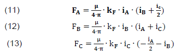
When determining electrodynamic interactions at three-phase faults, two cases can be distinguished taking into account or omitting the fact of non-periodic components. If the influence of non-periodic components is omitted, and assuming that the individual phase currents are directed in accordance, they can be described by the following formulas:
To correctly determine the value of mutual interaction of electrodynamic forces, the largest possible values of forces should be found, which in this case will occur for the maximum value of the multiplication of both currents. Therefore, in a flat single three-pole system, where the external current circuits are arranged symmetrically with respect to the middle busbar, the electrodynamic forces acting on individual conductors can be described by the following equations:
.
.
After proper substitution of the above formulas, the equation is obtained that allows to determine the value of electrodynamic forces acting on the external current circuits through which current iA flows:
.
To obtain the maximum value of force it is necessary to determine the extremes for the function f(ωt):
.
After substitution, the below equations are derived:
.
The maximum values of electrodynamic forces for the external current circuit through which the current iC flows are exactly the same as for the conductive busbar iA and could be determined from the following dependencies:
.
The value of electrodynamic forces acting on the center busbar of the system presents slightly different. After substituting the current formulas, the equation is obtained:
.
After determining the maximum values, the above dependency can be described as:
.
Numerical calculations
In low voltage switchgears, small insulation gaps between the busbars of individual phases are sufficient, and the level of short-circuit currents is similar to that in high voltage switchgears. The problem of electrodynamic stresses acting on busbars is therefore more pronounced in the former, although the mitigating circumstance is the smaller distances between the busbar fastening points. The rules for dimensioning rigid rails regarding electrodynamic loads in short-circuit conditions are specified in the standard (IEC 865-1 Short-circuit currents – Calculation of effects). The calculations are quite complex and based on such simplifications that their practical usefulness is not enough. When developing the concept of a new series of switchgears, those serve as the basis for initial design solutions, which are then verified in the short-circuit laboratory. Multicore cables and other insulated conductors, correctly selected for their thermal short-circuit endurance, generally also withstand the electrodynamic forces associated with the flow of short-circuit current. Due to the small thickness of the insulation, and therefore smaller distances between the axes of the conductors, the electrodynamic forces in cables and other low-voltage devices – with the same value of short-circuit current – are greater than in high-voltage cables. Checking may be needed in the case of extremely high short-circuit currents (over 60 kA) that are switched off in a short time (less than 20 ms), but without any limiting effect, i.e. with passing the expected value of the surge from short-circuit current.
Electrodynamic exposures must also be considered while choosing the construction principle and technique of assembly of the heads and cable joints.
The finite element method is a necessary and versatile – often used numerical method that can clearly optimize the process of designing electrical devices. The article proposes the use of FEM tools, such as SolidWorks and ANSYS, to support the design and modeling of high-current circuits and their contacts. The models were simulated taking emphasis on the electrodynamic forces analysis caused by the short-circuit current flow. At the model stage, physical phenomena important not only from the point of view of the mechanical properties, but also from the view of electrical engineering were determined. This procedure is unbelievably valuable during design/engineering work. That concerns mostly the material economy. Figure 1 shows a model of the current circuits of an exemplary low voltage switchgear with contacts. The model was made in the SolidWorks program.
Fig.1. Busbar model made in the SolidWorks program (cross-section of a single 60 x 10 mm busbar).
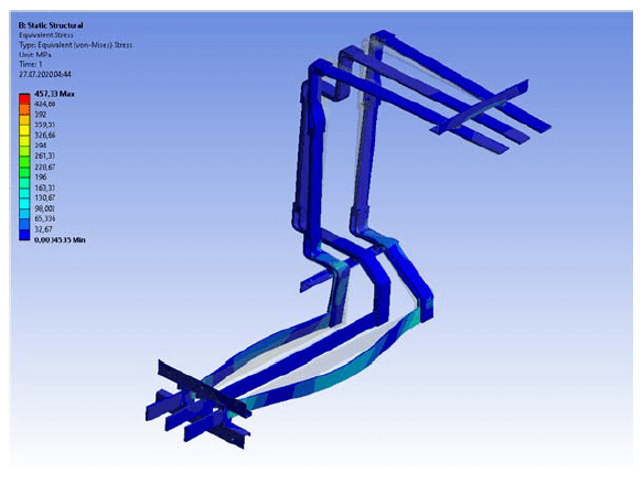
The model prepared in this way was subjected to the full modeling process in the ANSYS program. The boundary conditions and the correct exposure of the results were considered. Figure 2 shows the results of reduced stresses caused by the flow of a short-circuit current of 50 kA.
A series of numerical calculations were made to determine the electrodynamic force, and thus the maximum mechanical stresses. The simulations were made for a three-phase short-circuit current with the waveforms shown in Figure 4.
Fig.2. Reduced stresses resulting from the flow of short-circuit current.
Fig.3. The total stresses caused by the flow of the short-circuit current.
Fig.4. Waveforms of three-phase short-circuit current.
The presented results clearly show that it is worth stabilizing current circuits with support insulators. Despite the high electrodynamic forces (power supply lines), the mechanical stresses ought to be stabilized on the receiving lines. The risk of vibrations transmission to the supply devices is reduced, which is especially important for a rigid connection.
Summary
This work concerns building the FEM models that fully and faithfully reproduce real-world conditions. The given approach is invaluable when it comes to modeling electrical apparatuses. The selected approach was to use FEM tools to design not only arc chambers, contact systems but also high-current circuits. However, the optimal capabilities of the tools to which they are dedicated were used to obtain a valuable and complete picture of the modeled object. Indeed, it has been achieved. The presented model, as well as the procedure, have been verified by empirical studies that confirm the rightness of such proceedings. An important feature resulting from this work is the possibility of reconstructing models of designed objects and in the case of structural changes, avoiding expensive and time-consuming laboratory tests or at least reduce their costs. This approach is correct in view of the current trend to reduce time and costs in the design and manufacture process of electrical equipment. Optimization can be applied to existing solutions with the proposed procedure. Such a process can not only increase user safety/service quality, but also reduce material consumption, positively influencing the environment. In addition, FEM modeling can be used to design apparatuses for various conditions, voltage ranges and applications. The above gives great opportunities for safe, fast, and highly economical creation of new trends and solutions in electrical engineering. Of course, the disadvantage of FEM modeling is still the need to conduct experimental tests. More complex solutions may generate additional errors that often lead to inaccuracies in the obtained measurement series during simulation. This is especially expected when establishing boundary conditions. Nevertheless, it is worth using the proposed design tool.
REFERENCES
[1] Bini R., Galletti B., Iordanidis A., Schwinne M., 1st International Conference on Electric Power Equipment – Switching Technology – Xi’an – China, 2011, pp. 375-378 [2] Dhotre M.T., Ye1 X., Seeger M., Schwinne M., Kotilainen S., CFD Simulation and Prediction of Breakdown Voltage in High Voltage Circuit Breakers, 2017 Electrical Insulation Conference (EIC), Baltimore, MD, USA, 11-14 June 2017 [3] Jiaxin Y., Yang W., Lei W., Xiaoyu L., Huimin L., Longqing B., Thermal Dynamic Stability Analysis for the Enclosed Isolated – Phase Bus Bar Based on the Subsegment Calculation Model, IEEE Transactions on Components, Packaging and Manufacturing Technology, vol. 8, no. 4, April 2018, pp. 626-634 [4] Williams D.M., Human factors affecting bolted busbar reliability, in Proc. IEEE 62nd Holm Conf. Elect. Contacts (Holm), Clearwater Beach, FL, USA, Oct. 2016, pp. 86–93, October 2016 [5] Yang J., Y. Liu, D. Hu, B. Wu, Li J., Transient vibration study of GIS bus based on FEM, in Proc. IEEE PES Asia–Pacific Power Energy Eng. Conf. (APPEEC), Xi’an, China, pp. 1092–1095, October 2016 [6] Triantafyllidis D.G., Dokopoulos P.S., Labridis D.P., Parametric short-circuit force analysis of three-phase busbars-a fully automated finite element approach, IEEE Trans. Power Del., vol. 18, no. 2, pp. 531–537, April 2003 [7] Yang J., Liu Y., Hu D., B., Wu, Che B., Li J., Transient electromagnetic force analysis of GIS bus based on FEM, in Proc. Int. Conf. Condition Monitor. Diagnosis (CMD), Xi’an, China, pp. 554–557, September 2016 [8] Guan X., Shu N., Electromagnetic field and force analysis of threephase enclosure type GIS bus capsule, in Proc. IEEE PES T&D Conf. Expo., Chicago, IL, USA, pp. 1–4, April 2014 [9] Kolimas Ł., Łapczyński S., Szulborski M., Tulip contacts: experimental studies of electrical contacts in dynamic layout with the use of FEM software, International Journal of Electrical Engineering Education, vol. I, pp. 1-4, 2019, Early Access: https://doi.org/10.1177/0020720919891069 [10] Kolimas Ł., Łapczyński S., Szulborski M., Świetlik M., Low Voltage Modular Circuit Breakers: FEM Employment for Modelling of Arc Chambers, Bulletin of the Polish Academy of Sciences-Technical Sciences, vol. 68, no. 1, pp. 61-70, 2020 [11] Kolimas Ł., Łapczyński S., Currents of contact welding in a static layout: A laboratory exercise, International Journal of Electrical Engineering Education, I, ISSN 0020-7209, 2019, Early Access: https://doi.org/10.1177/0020720919840986 [12] Kolimas Ł., Łapczyński S., Szulborski M., Drogosz M., Kozarek Ł., Kędziora B., Wiśniewski Ł., Bieńkowski K., Simulations and Tests of a KRET Aerospace Penetrator, Energies, ISSN 1996- 1073, pp. 1-23, 2020 [13] Rumpler C., Stammberger H., Zacharias A., Low-voltage arc simulation with out-gassing polymers”, in Proc. IEEE 57th Holm Conf. Electr. Contacts, 2011, September, pp. 1–8 [14] Ryzhov V.V., Molokanov O.N., Dergachev P.A., Vedechenkov N,A,, Kurbatova E.P., Kurbatov P.A., Simulation of the Low – Voltage DC Arc, Intenational Youth Conference on Radio Electronics, Electrical and Power Engineering (REEPE), 14-15 March 2019, Russia [15] Bini R., Basse N.T, Seeger M., Arc-induced Turbulent Mixing in a Circuit Breaker Model, J. Phys D Appl Phys 44, vol. 2., 2011 [16] Basse N.T., Bini R., Seeger M., Measured turbulent mixing in a small-scale circuit breaker model, Appl. Optics, vol. 48, no. 32, 2009, pp. 6381-6391 [17] Incropera F.P., DeWitt D.P., Bergman T.L, Lavine A.S., Introduction to Heat Transfer, 5th ed. Hoboken, NJ, 2006, USA: Wiley [18] Muller P.T., Macroscopic electro thermal simulation of contact resistances, Bachelor thesis, RWTH, 2016, Aachen, Germany [19] Bini R., Basse N.T, Seeger M., Arc-induced Turbulent Mixing in a Circuit Breaker Model, J. Phys D Appl Phys 44, vol. 2., 2011 [20] Kolimas Ł., Łapczyński S., Szulborski M., Bieńkowski K., Kozarek Ł., Birek K, Control System and Measurements of Coil Actuators Parameters for Magnetomotive Micropump Concept, Bulletin of the Polish Academy of Sciences-Technical Sciences, vol. 68, no. 4, pp. 893-901, 2020. [21] Daszczyński T., Pochanke Z., Kolimas Ł., Uncertainty of the Characteristics of Electrical Devices Based on the Measurements of the Time-current Characteristics of MV Fuses, Bulletin of the Polish Academy of Sciences-Technical Sciences, vol. 68, no. 4, pp. 751-757, 2020.
Authors: dr inż. Łukasz Kolimas, Politechnika Warszawska, Instytut Elektroenergetyki, ul. Koszykowa 75, 00-662 Warszawa, Email: lukasz.kolimas@ien.pw.edu.pl; mgr inż. Sebastian Łapczyński, Politechnika Warszawska, Instytut Elektroenergetyki, ul. Koszykowa 75, 00-662 Warszawa, E-mail: seb.lapczynski@gmail.com; mgr inż. Michał Szulborski, Politechnika Warszawska, Instytut Elektroenergetyki, ul. Koszykowa 75, 00-662 Warszawa, E-mail: mm.szulborski@gmail.com.
Source & Publisher Item Identifier: PRZEGLĄD ELEKTROTECHNICZNY, ISSN 0033-2097, R. 96 NR 11/2020. doi:10.15199/48.2020.11.37
Published by Makmur SAINI1, A. M. Shiddiq YUNUS1, Ahmad Rizal SULTAN1, Muh Ruswandi DJALAL1, Mohd. Wasir bin MUSTAFA2, Rahimuddin RAHIMUDDIN3, Ikhlas KITTA3, State Polytechnic of Ujung Pandang (1), University Teknologi Malaysia (2), Hasanuddin University (3)
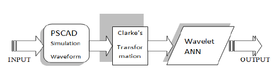
Abstract. This paper introduces a comparative study for fault detection and classification on parallel transmission line using cascade forward and feed forward back propagation. Both calculations were based on discrete wavelet transform (DWT) and Clarke’s transformation. Daubechies4 mother wavelet (Db4) was applied to decompose coefficients of wavelet transforms coefficients (WTC) and wavelet energy coefficients (WEC) of high frequency signals. The coefficients were inputs for training of neural network back-propagation (BPNN). The results showed that the feed forward back propagation algorithm of Artificial Neural Network (ANN) models responded better than Cascade forward back propagation algorithm models, particularly in fault detection and classification on parallel transmission. The results showed that the proposed method for fault analysis was able to classify all the faults on the parallel transmission line rapidly and correctly.
Streszczenie. W pracy przedstawiono badanie porównawcze wykrywania i klasyfikacji uszkodzeń równoległej linii przesyłowej z wykorzystaniem propagacji kaskadowej do przodu i do tyłu. Oba obliczenia oparto na dyskretnej transformacie falkowej (DWT) i transformacji Clarke’a. Falkę macierzystą Daubechies4 (Db4) zastosowano do dekompozycji współczynników przekształceń falkowych (WTC) i współczynników energii falkowej (WEC) sygnałów wysokiej częstotliwości. Współczynniki stanowiły dane wejściowe do szkolenia propagacji wstecznej sieci neuronowej (BPNN). Wyniki pokazały, że algorytm propagacji wstecznego sprzężenia zwrotnego modeli sztucznej sieci neuronowej (ANN) zareagował lepiej niż modele algorytmu kaskadowego propagacji wstecznej, szczególnie w wykrywaniu błędów i klasyfikacji w transmisji równoległej. Wyniki pokazały, że zaproponowana metoda analizy uszkodzeń była w stanie szybko i poprawnie sklasyfikować wszystkie uszkodzenia na równoległej linii przesyłowej. Wykrywanie błędów w równoległej linii przesyłowej z wykorzystanirem transformaty Clarke’a
Keywords: Cascade and Feed forward back-propagation neural network; Clarke’s Transformation; Fault detection; Fault Classification; Słowa kluczowe: Sieć neuronowa propagacji wstecznej i kaskadowej; Transformacja Clarke’a; Wykrywanie uszkodzeń; Falka
Introduction
Power transmission line is an essential element in power system as it can dispatch electrical energy from one place to another. However, faults are often occurred on the transmission lines due to the interferences. Moreover, short circuit at the transmission line that connected to the wind turbine for example, could damage the wind turbine generator and its power electronics device [1]. Therefore, a quick and accurate analysis is necessarily required to detect and classify the transmission lines faults to guarantee the high reliability of the power system. a parallel transmission line needs more special consideration in comparison with the single transmission line, due to the effect of mutual coupling on the parallel transmission line including a parallel transmission line that is connected with wind turbine [2]. The most advantage of the parallel transmission compared to the single line is the probability of parallel system to transmit power continuously during and after fault is better than the single line.
This paper proposed a discrete wavelet transform and back-propagation neural network using the Clarke’s transformation to detect and classify the faults on the parallel transmission line. This study proposes a new method called alpha-beta transformation that is based on the Clarke’s transformation; which is a transformation of a three-phase system into a two-phase system [3-6]. Clarke’s transformation result is then transformed into discrete wavelets transform.
Wavelet transforms have been applied in several applications of in power systems; for example on partial discharge, power system protection, power system transients, condition monitoring and transformer protection. Among aforementioned above, the power system protection become the major application area of wavelet transform in power systems [7], while the Artificial Neural Network has been widely used in power system protection [8]. In this study, a novel approach is proposed for some reliable fault detection, classification, and location. The proposed approach applied based on ANN scheme. Various types of faults were applied for classification of the faults and location [9]. There are some papers recently discussed the hybrid application of wavelet and ANN that have been applied on the variety of power system planning and power quality disturbances [10-13], estimating fault location [16], classification using Oscillographic data [14, 15], control system and state estimation [16, 17].
This study introduces a new approach for classifying faults in transmission lines using discrete wavelet transform and back-propagation neural network. The main idea of the approach is to employ wavelet coefficient detail and the wavelet energy coefficient of the currents as the input patterns to generate a simple multi-layer perception network (MLP). In addition, this study proposes the development of a new decision algorithm to be used in the protective relay for fault classification and detection. To validate this method, the applied faults were simulated using EMTDC / PSCAD software package [18]. Moreover, to obtain the significant of the study, the results of the proposed method were compared with and without wavelet transform based Clarke transformation.
Research Methodology
In this section Figure 1 shows the procedure of main steps for fault detection on transmission line using DWT and BPPN based on Clarke’s transform it also shows some tools like PSCAD/EMTDC, wavelet transform (WT) and back propagation neural network (BPNN) is used to detect and classify the faults.
Fig. 1. Flow chart for the proposed methodology
The design process of the proposed fault detection and classification algorithm for transmission line goes through the following steps:
1) Finding the input to the Clarke’s transformation and wavelet transform. The signal flow of PSCAD is then converted into m. Files (*. M) 2) Determining the data stream interference, where the signal is transformed by using the Clarke’s transformation to convert the transient signals into the signal’s basic current (Mode).
.
3) Input signals are analyzed by DWT for extracting the information of the transient signal in the time and the frequency domain [19]. 4) Selection of a suitable BPNN topology & structure for a given application. 5) Training of BPNN and validation of the trained BPNN to check its correctness in generalization.
Results and Discussion
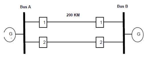
In this study, the system under study is consisted of two identical transmission lines of 200 Km length which both end side are connected to Bus A and Bus B respectively. Each bus is connected to identical generator. The system was built on a 230 kV, conducted and simulated using PSCAD/EMTD. The system under study is shown in Fig. 2. In this study faults are applied at 0.22s and last for 0.15s and system under study parameters are provided in Table 1.
Table 1. Parameters used in the model System under Study
.
Fig. 2. Single line diagram of the system under study
After calculating the parameters, the training sample of the detail coefficients wavelet of S0,Sα, Sβ, Sγ, Q0,Qα, Qβ, Qγ and wavelet energy of E0 , Eα, Eβ and Eγ for various types of faults were set as input variables to create neural network. The data sets were generated by considering different operating conditions, for examples, the different values of initiation angles ranging between 0 and 180 degrees, different values of fault resistances are set between 0 and 200 ohm and different fault distances from 0 to 200 km. The fault types are AG, BG, CG, ABG, BCG, ACG, AB, BC, AC, and ABC, where fault locations for training and testing are assumed occurs at 25, 50, 75, 100, 125, 150 and 175 km. For training and testing of Fault Resistance (Rf) are determined as: 0.001,25, 50, 75, 100, 125, 150, 175 and 200 ohm, whilst Fault Inception Angle for training and testing are set at: 0, 15, 30, 45, 60, 90, 120, 150 and 180 degrees. From the simulation results, it can be stated that the proposed DWT and BPNN were able to accurately distinguish among the ten possible categories of faults. The truth table representing the faults and the ideal output for each of the faults is illustrated in Table 2.
WTC and WEC Based Fault Classification and Detection
DWT is one of mathematical tools that can be used to detect fault. In this approach, each of the derived current fault signals was decomposed into its constituent wavelet sub-bands or levels by the mother wavelet (Db4). The 4 levels of frequency bands are mentioned as dl, d2, d3 and d4. The high frequency components will be increased from d4 to d1. The wavelet coefficients detail of the currents was filtered using Clarke transformation, as exhibit in Fig. 3, while Fig. 4 shows the filtering response without using Clarke transformation. By applying aforementioned rules above, the first and last faulted samples were found at 105 respectively, for a sampling frequency of 200 kHz.
Table 2. The truth table representing the faults and the ideal output for each of the faults
.
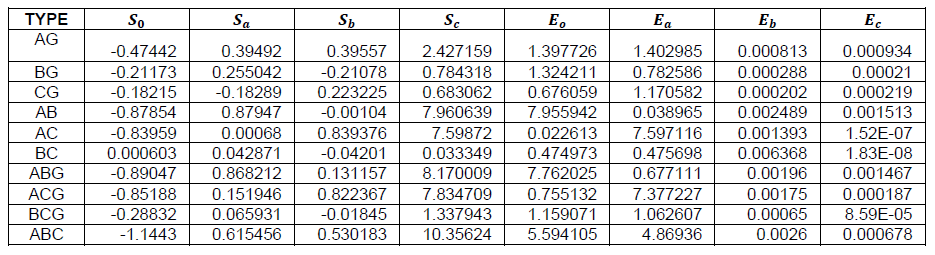
From the sum of square of detailed WTC, we can obtain the WEC [25]. The wavelet energy coefficient varies over different scales depending on the input signals. Wavelet energy coefficients E0 , Eα, Eβ and Eγ correspond to the sum of the four levels of wavelet energy coefficients of mode currents I0 , Iα, Iβ and Iγ with Clarke’s transformation, as exhibits in Table 3, while E0 , Ea, Eb and Ec correspond to the sum of the four levels of wavelet energy coefficients of line currents I0 , Ia, Ib and Ic without Clarke’s transformation as can be seen in Table 4.
Results of using DWT and Feed Forward Back Propagation Network (FFBPPN)
After calculating the parameters, the training sample of the detail coefficients wavelet various parameters of S0,Sα, Sβ, Sγ, Q0,Qα, Qβ, Qγ and wavelet energy of E0 , Eα, Eβ and Eγ for various types of faults were set as input variables to create neural network. The data sets were generated by considering different operating conditions, for instant, the different values of inception angles ranging between 0 and 180 degrees, different values of fault resistances between 0 and 200 ohm and different fault distances from 0 to 200 km. Discreet combination (A-B-C-G) of faults classification obtained by defining 1 for the value more than 0.6 and 0 for the value less than 0.4. The simulation results are shown in Table 3. Error percentage of combination using preprocessing Clarke’s transformation compared to without Clarke’s transformation calculated as follows:
Percentage of MSE Validity =
.
Percentage of MAE Validity =
.
where MSE (WoTC) is Mean Square Error (MSE) Without Clarke’s Transformation and MSE (WiTC) is Mean Square Error (MSE) With Clarke’s Transformation .MAE (WoTC) is Mean Absolute Error (MSE) Without Clarke’s Transformation, and MAE (WiTC) is Mean Absolute Error (MSE) With Clarke’s Transformation.
Simulation result of fault classification and detection using DWT and Feed-forward BPPN performing better results when analysis with preprocessing using Clarke’s transformation and architecture combination of 12-12-24-4 (12 neurons in the input layer, 2 hidden layer with 12 and 12 neurons in them, respectively and 4 neurons in the output layer). The results of the training performance plot of the neural network are shown in Fig. 3 and Fig. 4.
Fig.3. Level 4 DWT coefficient detail of the fault (AG) at 125 km, signalled with Clarke’s transformation
Fig.4. Level 4 DWT coefficient detail of the fault (AG) at 125 km, signalled without Clarke’s transformation
Table 3. Detail of Wavelet Coefficient and Wavelet Energy Coefficient in Fault Location at 125 Km, Fault Resistance=100 Ohm and Inception at Angle 30 Degree with Clarke’s Transformation
.
Table 4. Detail of Wavelet Coefficient and Wavelet Energy Coefficient in Fault Location at 125 Km, Fault Resistance=100 Ohm and Inception at Angle 30 Degree without Clarke’s Transformation
.
Fig.5. Fit Regression of the Outputs vs. Targets of Feed-forward BPPN with configuration (12-12-24-4) without using Clarke’s transformation.
Fig.6. Fit Regression of the Outputs vs. Targets of Feed-forward BPPN with configuration (12-12-24-4) with Clarke’s transformation
Fig.7. Fit Regression of the Outputs vs. Targets of Cascade-forward with configuration (12- 12-24-4) without using Clarke’s transformation
Fig.8. Fit Regression of the Outputs vs. Targets of Cascade-forward with configuration (12- 12-24-4) with using Clarke’s transformation
The results of DWT and BPNN training without Clarke’s transformation shown that MSE is 0.056214 and MAE is 0.154754, and with Clarke’s transformation show that MSE is 0.053876 and MAE is 0.150301. Percentage of MSE Validity obtains about 4.159 % and MAE obtains about 2.877 % compare to without preprocessing Clarke’s transformation and plotting of the best linear regression that relates the targets to the outputs are shown in Fig.5 and Fig. 6.
Results of using DWT and Cascade Forward Back Propagation Network (CPBPPN)
Similar to the feed Forward Back propagation Network, the parameters of the training of the detail coefficients of wavelet has various parameters, namely S0,Sα, Sβ, Sγ, Q0,Qα, Qβ, Qγ and wavelet energy E0 , Eα, Eβ and Eγ for various types of faults were set as input variables of the neural network. The data sets were generated by considering the different operating conditions, for example, the different values of inception angles are ranging between 0 and 180 degrees, different values of fault resistances are varied between 0 and 200 ohm and different fault distances take places from 0 to 200 km. Discreet combination (A-BC- G) of faults classification obtained by defining 1 for the value more than 0.6 and 0 for the value less than 0.4.
The results of DWT and BPNN training without Clarke’s transformation, it found that MSE is 0.073929 and MAE is 0.1421057. Meanwhile, with Clarke’s transformation, where the MSE is found to be 0.062201 and MAE is 0.129653, Percentage of MSE Validity achieves about 15.863 % and MAE for about 8.763 % compare to without preprocessing Clarke’s transformation. The plotting of the best linear regression that relates the targets to the outputs are shown in Fig. 7 and Fig.8. The simulation results for various neural network combination / architecture were presented in Table 5. The feed forward back propagation network shows better performance with the MSE and MAE have lesser error compared to the performance of Cascade forward back propagation network. It is shown that the MSE and MAE of FFBPPN have a smaller value than CPBPPN. By adopting Clarke’s transformation, it was yielded that MSE and MAE have smaller value compared to the network without Clarke’s transformation on FFBPPN and CPBPPN. Among all the architectures, the best architect was 12-24- 48-4.
Conclusion
This paper is aimed to compare and explore the practicability of Feed forward back propagation and Cascade forward back propagation network in ANN models in order to recognize fault classification and detection on parallel transmission lines. This approach applies Daubechies4 (db4) as a mother wavelet. Various circumstances have been investigated, including variation on distance, fault resistance and the initial angle.This study also compare the results of training BPPN and DWT with and without Clarke’s transformation, where the results exhibits that using the Clarke’s transformation in training will create smaller MSE and MAE, compared to training without Clarke’s transformation. Among the three structures, the best architects result is 12-24-48-4. The Feed forward back propagation algorithm of Artificial Neural Network (ANN) models performed better results than Cascade forward back propagation algorithm models, particularly in fault classification and detection on parallel transmission lines.
Acknowledgment
The authors would like to thank Research, Technology and Higher Education Ministry of Indonesia for supporting the Research.
REFERENCES [1] A. M. Shiddiq Yunus, A. Abu-Siada, and M.A.S. Masoum, Improving dynamic performance of wind energy conversion systems using fuzzy-based hysteresis current-controlled superconducting magnetic energy storage, IET Power Electronics, 5(8), pp. 1305-1314. 2012. [2] A. M. Shiddiq Yunus, A. Abu-Siada, and M.A.S. Masoum, Effects of SMES on dynamic behaviours of type D-Wind Turbine Generator-Grid connected during short circuit. IEEE Power and Energy Society General Meeting, 6039276. 2011. [3] B. Polajzer, G.s. Tumberger, S., Seme, D Dolinar, Detection of voltage sources based on instantaneous voltage and current vectors and orthogonal clarke’s transformation, IET. Gener .Transm. Distrib, 2,(2), 219–226, 2008. [4] Chaari,M. Meunier, F. Brouave, Wavelet a new tool for the resonant grounded power distribution systems relaying, IEEE Trans. on Power Delivery, Vol. 11 , (3), 1301-1308. 1977. [5] Jamian, J.J., Mohd Zin, A.A., Saini, M., Mustafa, M.W., Mokhlis, H., A Novel TVA-REPSO technique in solving generators sizing problems for South Sulawesi Network, Przeglad Elektrotechniczny, Vol. 89, Issue 2 A, pp. 170-174, 2013. [6] Saini, M., Mohd Zin, A.A., Mustafa, M.W., Sultan, A.R., Nur, R., Algorithm for fault location and classification on parallel transmission line using wavelet based on Clarke’s transformation. International Journal of Electrical and Computer Engineering, Vol. 81, Issue 2, pp. 699-710. 2018. [7] C.H. Kim, R. Aggarwal, Wavelet transforms in power systems, IET Power Engineering Journal, 15, 193-200, 2001. [8] Y.H. Song, A.T. Johns, Q.Y. Yuan, Artificial Neural Network based Protection Scheme for Controllable Series compensated EHV Transmission Lines, IEE Proc. on Gener., Transm. and Distr, 143, 2032-2040. 1996. [9] J.Ezquerra, V. Valverde,I. Mazo´n, A.J. Zamora, JJ Zamora, Field programmable gate array implementation of a fault location system in transmission lines based on artificial neural networks, IET Gener. Transm. Distrib, 5, (2), 191– 198, 2011. [10] W.J.Cheong, R.K.Aggarwal, Accurate fault location in high voltage transmission systems comprising an improved thyristor controlled series capacitor model using wavelet transforms and neural network, Transmission and Distribution Conference and Exhibition, 2, 840–845, 2000. [11] R.G.Maryam, M.R.istr Shakarmi, F.Namdari, Detection and classification power quality distribunce using neural Network based discrete wavelet trandform, J. Electrical Systems, 12 (1), 158 – 173, 2016. [12] P. Chiradeja, A. Ngaopitakkul, Prediction of Fault Location in Overhead Transmission Line and Underground Distribution Cable Using Probabilistic Neural Network, P. Chiradeja, A. Ngaopitakkul, International Review of Electrical Engineering. Vol 8, No 2 (2013), pp. 762-768. 2013. [13] Sudha Gopal, Valluvan K. R, A Novel Approach to Fault Diagnosis of Transmission Line with Rogowski Coil, International Review of Electrical Engineering. Vol 9, No 3, pp. 656-662. 2014 [14] Y. Menchafou1, M. Zahri, M. Habibi, H. E. Markhil, Extension of the Accurate Voltage-Sag Fault Location Method in Electrical Power, J. Electrical Systems, 12(1), 33 – 34, 2016. [15] K.M.Silva, B.A. Souza, N.S,D. Brito, Fault Detection and Classification in Transmission Lines Based on Wavelet Transform and ANN’, IEEE Trans. on Power Delivery, Vol. 21 (4). 2058-2063, 2006. [16] F.B. Costa, K.M. Silva, B.A. Souza, K. M. C., Dantas, N. S. D. Brito, A Method for Fault Classification in Transmission Lines Based on ANN and Wavelet Coefficients Energy, International Joint Conference on Neural Networks, Sheraton Vancouver Wall Centre Hotel, Vancouver, BC, Canada, July 16-21, 2006. [17] I.K.Yu, Y.H.Song, Wavelet analysis and neural networks based adaptive single pole auto reclosure scheme for EHV transmission systems, International Journal of Electrical Power & Energy Systems, pp. 465–474, 1998. [18] L.L. Lai, F. Vaseekar, H. Subasinghe, N. Rajkumar, A. Carter, B.J. Gwyn, , Fault location of a teed-network with wavelet transform and neural networks’, in: DRPT International Conference on Electric Utility Deregulation and Restructuring and Power Technologies, pp. 505–509, 2000 [19] B. Alberto, B. Mauro, D. Mauro, A. N.Carlo, P.Mario, Continuous-Wavelet Transform for Fault Location in Distribution Power Networks: definition of mother wavelet inferred from fault originated transeient , IEEE Trans. on Power Delivery, Vol 23,No 2, May 2008, pp. 380-389
Authors: Prof. Makmur Saini is with Power Generation Engineering Study Program, Mechanical Engineering Department, State Polytechnic of Ujung Pandang, Makassar 90245, Indonesia, Email: makmur.saini@poliupg.ac.id; Dr. A. M. Shiddiq Yunus is with Energy Conversion Study Program, Mechanical Engineering Department, State Polytechnic of Ujung Pandang, Makassar 90245, Indonesia, Email: shiddiq@poliupg.ac.id; Dr. Ahmed Rizal Sulthan is with Electrical Engineering Department, State Polytechnic of Ujung Pandang, Makassar 90245, Indonesia, Email: rizal.sultan@poliupg.ac.id; Muh.Ruswandi Djalal, MT is with Power Generation Engineering Study Program, Mechanical Engineering Department, State Polytechnic of Ujung Pandang, Makassar 90245, Indonesia, Email : wandi@poliupg.ac.id; Prof. M. W. Mustafa, University Technology Malaysia, Email:wazie@fke.utm.my, Dr. Rahimuddin, Naval Engineering Department, Hasanuddin University, Gowa, Indonesia, Email: rahimnav@gmail.com; Ikhlas Kitta, Electrical Engineering Department, Hasanuddin University, Indonesia, Email: ikhlaskitta@gmail.com;
Source & Publisher Item Identifier: PRZEGLĄD ELEKTROTECHNICZNY, ISSN 0033-2097, R. 96 NR 4/2020. doi:10.15199/48.2020.04.04
Published by Marcin KOPYT, Warsaw University of Technology, Electrical Power Engineering Institute
Abstract. Electricity demand predictions are one of the most important tools used for Power System work planning. However, a departure from traditional solutions seems to be inevitable in the light of ever-increasing RES share. This paper is the second of a two-part extensive review of recent literature related to forecasts of RES generation, electricity demand and power flows, and presents the second and third of the mentioned aspects.
Streszczenie. Prognozy zapotrzebowania na energię są jednym z najważniejszych narzędzi w Planowaniu pracy SEE. Odejście od ich klasycznych rozwiązań wydaje się być jednak nieuniknione w świetle coraz bardziej zwieszającej się liczby OZE. Niniejszy artykuł to druga z 2 części szerokiej analizy najnowszej literatury dotyczącej prognoz generacji z OZE, zapotrzebowania i przepływów mocy. Prezentuje on 2 i 3 aspekt. Prognozy przepływów mocy-przegląd status quo. Część 2: Predykcja zapotrzebowania na energię i przepływów mocy.
Keywords: forecasting, demand, RES, power flows Słowa kluczowe: prognozowanie, zapotrzebowanie, OZE, przepływy mocy
Introduction
This paper is the second part of an extensive review concerning various aspects of power flow forecasts – Power Flow Forecasts: A Status Quo Review. Due to significant amount of material to be presented, the paper is divided into two parts. The first part pertains to predictions of generation, while the second addresses electricity demand & power flows forecasts.
The rationale for this review and broader introduction is provided in the first part of this paper. This second part structures the aspects discussed in the literature, characterizes their common features, key differences and inconveniences associated with them. Forecasts of electricity demand Recent studies addressing electricity demand predictions can be divided into seven categories:
a) System electricity demand predictions b) Electricity demand predictions for an area c) Multinodal demand forecasts d) Building demand forecasts e) Peak load forecasts f) Long-term electricity demand with price elasticity analyses g) Analyses of climate influence on long-term load forecasts
System electricity demand predictions
Dudek [1] proposes the Theta method for the prediction of electricity demand in the Polish Power System. A variant of exponential smoothing, it is remarkable for its simplicity and accuracy of prediction of processes of varying nature and frequencies. The author compares the method in its standard (STM) and dynamically optimized (DOTM) variants. He takes into consideration both a singular model which forecasts 24-h ahead, and 24 parallel models, each forecasting 1 h of a 24-h period. Out of all variants, ARIMA was the least accurate, while the rest of the models yielded similar results.
Authors second work [2] considers more countries as test sample. For purpose of forecasting monthly electricity demand of Polish, German, French and Spanish power systems, k nearest neighbor method was proposed. First considered model forecasts 12 months ahead, while second one is consisted of 12 submodels, each forecasting one chosen month ahead. Method simplicity could be treated as its advantage.
Among the publications from 2017-2019 concerning forecasts of system electricity demand, no papers were found proposing solutions for three different time scales, as was the case, for example, in [3]. Of course, the collected materials do not cover the entire pool of work, but it may be an indication that creating comprehensive solutions is or is becoming a niche.
Electricity demand predictions for areas
The main difference between area and system load forecasting is scale. Obviously, tests of methods applied to one set of data can yield a different magnitude of error on another set, due to, for instance, different RES penetration in the regional and whole-system scale, or different consumer concentration. Nonetheless, it is easier to perform tests on many discrete regions than on entire systems. Data acquisition can be potentially easier, too. Some studies were carried out on that subject [4-11] and the number of regions on which models were tested ranged from 1 to 7.
For regional forecasts, the most popular solution were hybrid and combined models using ANNs as a component [4-10]. Statistical models were relatively rare [11]. For regional power demand predictions, Gong et al. [4] propose Seq2Seq, used by default as a text machine translation tool. In this solution, LSTM network is used as an encoder and decoder for feature extraction. To limit dimensionality of encoder output, selective learning of outputs (Attention Mechanism) is used. Predictions are generated by RLSTM network, modified to avoid overlearning.
Rodrigues & Trindade [5] propose a different, albeit equally interesting approach. Using functional clustering, they divide similar curves of daily loads by their phase and amplitude. For each group of curves, ELM models were created, after which final forecasts were taken as an average of such ensemble of forecasts. It should be noted that the method was tested in a climatically homogenous area, which excluded the need to analyze influence of factors like temperature on forecasts. This, however, could become a limiting factor if one wanted to use this solution on a larger scale.
An interesting example of a combined model is put forward in [6]. Its parallel CNN–LSTM model combines the generalization capability of CNN and long-term dependencies mapping capability of LSTM. Final predictions were obtained with feature-fusion module.
In their study, Ghadimi, Akbarimajd, Shayeghi & Abedinia [7] also use 2 combined ANNs. In this case, however, it is Ridgelet NN and ENN. Modified transductive model is used for data filtration, while the predictions engine consists of two parts. RDNN generated forecasts and is followed by ENN taking the role of error correction module.
Li, Yang, Li & Su [8] propose an even more complex method. EEMD is used to decompose data into trend, waveform and noise. GRNN learns to predict future waveform component split further into waveform with no seasonal component and residuum. Meanwhile, trend component was forecast by SVR optimized by PSO. Final prediction is obtained by recombining the waveform and the trend.
Xiao, Shao, Yu, Ma & Jin [9] additionally test the flexibility of their model by checking its performance in predicting wind speed and electricity price in the short term. Their approach is based on data decomposition by SSA and forecasting by WNN, optimized with rather advanced CS(BFGS-CS) method. The accuracy of prediction in this case is several dozens of percentage points better than for traditional BPNN.
Another example of GRNN use is put forward in [10]. For short-term forecasts, the authors use such network, for which the spread parameter is optimized by Fruit Fly Algorithm with Decreasing Step (SFOA). However, the change brought by adding Decreasing Step has not brought meaningfully better results than a model without it.
Unlike prior contributions, paper [11] suggests the use of a two-stage SARIMAX method. The goal of the first stage is to deal with SARIMAX problems, i.e., long execution time and discarding the outliers, and was done by reg-plussarma procedure. Suspicious regression errors are detected and transformed into their estimates. For determining the order of polynomials, the estimated regression errors are treated as a dependent variable. In the second step, the SARMA model is treated as benchmark, while the best SARMAX model is found by brute-search of increasing or decreasing the order of each SARMA polynomial and treating it as SARMAX model. Authors claimed that their procedure improves the goodness of fit for SARMAX.
In the work of Sowiński [12] end-use model is used. First, electricity consumption rate per capita for Poland and its voivodship is obtained by employing four stochastic differential equations models. Then, total demand of regions and country is being calculated by multiplying received per capita rates by predicted population size for given year and region. This approach allows to make distinction between industrialization level of different regions.
Multinodal demand forecasts
Studies on the subject such as [13,14] described rare cases of research studies on multinodal forecasts of load. In [13], for predicting the load of 9 substations, fuzzy-ARTMAP neural network with global load participation factor is used. The approach consists in a global load forecasting model and smaller local models, one per substation. Local models were parallel to each other, and their input was fed by the output from the global model and by the participation factor for the time of forecast, as well as for two previous hours. Such solution can coordinate forecasts on different hierarchy levels, and as a result increase the accuracy of nodal forecasts. FANN could be used even for much greater number of nodes, due to architectural stability of that model.
Paper [14] builds and develops on [13]. Unlike in a standard learning process, in [14] the output category is mapped to the input category, called “reverse training”. The purpose of that method is to reduce the error inherent in standard training.
Building demand forecasts
Papers on building load forecasting [15-18] have started appearing in a rather shy manner in recent years. The method put forward in [15] was meant to be an assistance tool for building EMSs. Based on hourly air temperature and humidity forecasts, probabilistic forecasts of temperature bounds and calendar data ANN and peak abnormal differential load models were developed. Those were later combined into a single probabilistic model of interval load prediction.
In contrast to previous work, the goal of [16] was to forecast not for one big, but for three small buildings. Studies involved data decomposition by SWEMD, extraction of features by Pearson correlation-based method and forecasting by ENN network optimized by NSSO algorithm.
Even more objects were analyzed in [17]. For five households, optimal time resolution was checked for different spatial resolution of forecasts (appliance-level/ zone-level/household-level). The time resolution was 30/60/120 minutes, and the zone-level referred to household rooms. Analyses were followed by forecasts of household power demand and power aggregated from individual predictions made for lower spatial levels. Bottom-up approach with Kalman’s Filter is used to achieve sufficient generalization capability, while results were compared to forecasts made by LSTM network, which shows an overall worse performance. The proposed approach is an intriguing change in treating human behavior as unpredictable by default and it could be potentially integrated into microgrid assistance tools.
Different buildings were chosen by authors of [18]. Their focus were office buildings. This resulted in less unpredictable behavior of consumer to be included in study. The method was designed with DSR in mind, and for that purpose SVR model was used.
Peak load forecasts
This aspect of demand forecasting is discussed in [19- 21]. For predictions of demand on the province level, Dai, Niu & Li [19] use advanced decomposition method, CEEMDAN, followed by a forecasting engine composed of SVM optimized by MGWO. CEEMDAN was used to eliminate noise from data while GWO was modified to eliminate getting stuck at local optima.
Elamin & Fukushige [20] use quantile regression for a similar purpose. Following regression, the value of the first quantile is computed based on the preceding quantiles. Based on this, the upper bound of demand peaks can be determined and blackouts due to underforecasting can be mitigated.
An interesting hybrid is put forward by authors of paper [21]. They propose grey systems and MVO optimizer, based on multiverse stability theory. MVO yielded better results than PSO and FOA.
Long-term electricity demand with price elasticity analyses and studies of the influence of climate on long-term load forecasts
Besides the main area of focus, some papers considered additional factors like historical price elasticity [22] or climate influence on electricity demand [23]. The solution suggested in [22] would be interesting for DSR analyses while [23] proves well-known correlations between weather and electricity demand. Correlations proved to be high for temperature and low for air humidity. In both mentioned works, ANN and fuzzy logic were used.
Features of electricity demand forecasts
Common features of studies on electricity demand predictions include the following:
a) Short horizon spanning from 1 to 24 h for most of papers b) Rare use of longer horizons, usually extending up to 9 days c) Occasional publication of medium-term predictions d) Advanced decompositions being one of the most important parts of models, with EMD variants being most popular e) Common use of ANNs as a prediction tool f) Regional electricity demand being the most popular topic g) Unexplored yet extensively multinodal demand forecasts h) Novelty such as the re-emergence of building demand forecasting i) Predominant use of hybrid and combined methods
The features of different aspects mentioned above are summarized in Table 1.
Power flow forecasts
Recent literature related to the subject of this section feature two predominant categories of research:
a) Models of dependences between load flows and RES generation [24-26] b) Net energy forecasts [27-32]
Models of dependencies between load flows and RES generation
Studies on the subject involve models developed, i.a., for better dispatch of power from conventional sources. This type of papers is based on corrections of load flows achieved in various ways. Prusty & Jena [24] correct PLF for a system with connected PVs with the use of previously developed time-space interdependencies model for objects. FFT and PCA methods were used as a base for this model, while GARCH model was used for predictions, which included time variability of standard deviation of residua. The influence of different RES was studied by Fang, Hodge, Du, Zhang & Li [25]. Based on historical time series of WT generation prediction errors, these researchers developed a sparse correlation covariance matrix to map time-space correlations between forecasts for turbines. With such matrix, a new set of equations, inequalities and constraints was defined for load flows. For the proposed solution, it was possible to control the parameter responsible for system resilience to WT demand instability. Kathiravan & Devi [26] made similar, albeit bit more extensive studies. Not only WTs, but also solar and heat&solar sources were included in their research. For each source, the authors determined a cost function which incorporated a penalty for deficits of fed power and incentives for surplus generation in case of power deficit. Both penalties and incentives were considered only after passing a specific threshold of prediction error introduced in calculations. Net energy predictions Massidda & Marrocu [27] forecast two variables. One is power exchanged with the network operator by the islandbased grid. The second variable was net load resulting from aggregate value of load and local, small PV generation. For their studies, the authors used historical values of forecasted values, sinusoidal functions reflecting seasonal changes and weather forecasts. SVR with RBF kernel was used as a final prediction tool.
Haupt et al. [28], in turn, studied the multinodal aspect of net load forecasts for distributed PVs. With the use of weather measurements, calendar and astronomical data, they developed parallel models of PV generation and electricity demand. In this approach, the output from PV generation is used as input for the second model. NWPs were used to correct the bias of the above-mentioned methods. This type of research demonstrates problems with acquiring data from different sources and is an example of creative solving of such problems. To make up for the lack of generation history for an area where PVs were located, the authors calculated the power based on weather conditions for meteo measurement stations, and later upscaled the results in proportion to total power capacity installed around the stations. For predictions of output % power regression, a tree model with the nearest neighbor correction is used.
Kaur, Nonnenmacher & Coimbra [29] based their research on net load forecasts for a University grid. With the help of SVR, two prediction variants were analyzed. Under the first one, demand and generation of University’s PVs were calculated in parallel and then added up together to calculate net demand. In the second approach, generation forecast was used as input to the net demand prediction model. The advantage of these studies is factoring in the influence of environmental factors on panel degradation. The fact that University HVAC was programmed and nondependent on users, which is not standard behavior of such systems, was, however, a sort of obstacle for transferability of the recommended solution.
An interesting combined model is put forward by Sepasi et al. [30]. For one substation, the authors generated predictions of net demand to improve energy management of BESS connected to substation. CVNN was used for forecasting, whereas the combined model is composed of two submodels, for simplicity called A and B here. Model A is responsible for parallel calculations for each hour of horizon. It was fed with historical data of similar day-types. Model B forecast the values for next hour based on current load and measurement going as far as 20 time-steps backwards. Certain hours of horizon measurements would not be available, therefore for these hours the output of model A was used. Day-type and Single hours decomposition used for model A could potentially allow for better pattern extraction, while the use of model B could better catch the time trend. With an increase in time step, however, the quality of the combined model would deteriorate due to forecast values replacing measurements.
Wang et al. [31] suggest another solution, this time based on probability. The following workflow is suggested. First, net load measurements are split into PV generation, actual load and residuum. Next, with the help of Kendall’s rank correlation, coefficient dependencies between the split models were determined. Based on the results of chi-square test, a copula function was chosen and parametrized with the mentioned coefficient. That way, the distribution of dependencies between models was determined, and final predictions were generated by convolution of forecasting error distributions.
Unlike previously mentioned papers which included only PVs in their net load studies, Li et al. [32] also include WTs. A comparison is made between two parallel additive models and one model explicitly forecasting net load. A model construction is suggested to allow for real-time re-optimization of model parameters in case of relative error increase over given time. In such model, rough optimizations are made by grid-search algorithm to save time, and re-optimization with genetic algorithm was used for fine tuning. The proposed solution is viable only with reliable, regular, and quick access to real-time measurement data, which limits its possible uses. Moreover, the longer the horizon, the more benefit is lost, reliable, regular, and quick access to real-time measurement data, which limits its possible uses. Moreover, the longer the horizon, the more benefit is lost,
Table 1 Aspects of electricity demand forecasts in literature
.
Table 2 Aspects of power flows forecasts in literature
.
Features of studies on power flow predictions or net demand predictions
The papers presented above have the following features:
a) Forecast interval was short and ranged from 5 min to 1h. b) Not all studies determined the horizon, but where they did, it ranged from 1h to 7 days. c) Net power forecasts remain not extensively explored, while a part of the research is related to dispatch scheduling from conventional sources. d) Net load predictions concerned usually systems with connected PVs. e) Two competitive approaches used in studies were additive models of RES generation and actual load prediction in parallel vs cascade model, where RES generation prediction was used as input to the net load forecasting model.
The features of different mentioned aspects are summarized in Table 2.
Summary
Recent studies have demonstrated that for electricity demand forecasting, various scales of research can be of interest either as a distinct area of study or as a “warm-up“ before model universality tests.
Re-emergence of forecasting of building demand deserves some attention as a change from narrative where consumer behavior is unpredictable. This could be a potential milestone in developing a bottom-up & top-down consistent demand and/or generation forecasting system.
Power flow forecasts in recent literature are rare and when they do appear, they tend to be connected with this subject rather loosely. Obviously, forecasts of such processes are more complex than forecasts of demand/generation only, but this fact plays rather minor role, hence it should not be the most limiting factor for studies.
It can be noticed that two approaches started to crystallize out of power flow studies, albeit superiority of one approach over another cannot be confirmed without new studies in the future.
It seems reasonable that effective development and use of predictions would attract attention in light of increasing RES penetration into power systems, the rise of electric cars and their charging stations.
.
.
REFERENCES:
[1] Dudek G, Short-term load forecasting using Theta method, 14th International Scientific Conference “Forecasting in Electric Power Engineering” (PE 2018)E3S Web of Conferences 84, 01004 (2019), https://doi.org/10.1051/e3sconf /20198401004 [2] Dudek G., Pełka P., Prognozowanie miesięcznego zapotrzebowania na energię elektryczną metodą k najbliższych sąsiadów, Przeglad Elektrotechniczny 1(4), (2017), 64-67 [3] Popławski T., Dudek G., Łyp J., Forecasting methods for balancing energy market in Poland, Electrical Power and Energy Systems, 65 (2015) 94–101 [4] Gong G., An X, Mahato N.K , Sun S., Chen S.,Wen Y., Research on Short-Term Load Prediction Based on Seq2seq Model, Energies, 2019, 12, 3199 [5] Rodrigues F., Trindade A., Load forecasting through functional clustering and ensemble learning, Knowl Inf Syst, 57 (2018), 229–244 [6] Tian C., Ma J., Zhang C., Zhan P., A Deep Neural Network Model for Short-Term Load Forecast Based on Long Short-Term Memory Network and Convolutional Neural Network, Energies,11 (2018), 3493 [7] Ghadimi N., Akbarimajd A., Shayeghi H., Abedinia O., Two stage forecast engine with feature selection technique and improved meta-heuristic algorithm for electricity load forecasting, Energy, 161 (2018), 130-142 [8] Li W., Yang X., Li H. ,Su L., Hybrid Forecasting Approach based on GRNN Neural Network and SVR Machine for Electricity Demand Forecasting, Energies, 2017, 10, 44; [9] Xiao L.,Shao W.,Yu M., Ma J., Jin C., Research and application of a hybrid wavelet neural network model with the improved cuckoo search algorithm for electrical power system forecasting, Applied Energy, 198(2017),203-222 [10] Hu R., Wen S., Zeng Z., Huang T., A short-term power load forecasting model based on the generalized regression neural network with decreasing step fruit fly optimization algorithm, Neurocomputing, 221 (2017), 24–31 [11] Tarsitano A., Amerise I.L., Short-term load forecasting using a two-stage sarimax model, Energy, 133 (2017), 108-114 [12] Sowiński J., Forecasting of electricity demand in the region, E3S Web of Conferences 84, 01010 (2019), https://doi.org/10.1051/e3sconf /20198401010 [13] Abreu T., Amorim A. J., Santos-Junior C.R., Lotufo A.D.P., Minussi C.R., Multinodal load forecasting for distribution systems using afuzzy-artmap neural network, Applied Soft Computing, 71 (2018), 307–316 [14] Amorim A.J., Abreu T.A., Tonelli-Neto M.S.,Minussi C.R., A new formulation of multinodal short-term load forecasting based on adaptive resonance theory with reverse training, Electric Power Systems Research, 179 (2020), 106096 [15] Xu L., Wang S., Tang R., Probabilistic load forecasting for buildings considering weather forecasting uncertainty and uncertain peak load, Applied Energy, 237 (2019), 180–195 [16] Mohammadi M., Talebpour F., Safaee E., Ghadimi N. Abedinia O., Small-Scale Building Load Forecast based on Hybrid Forecast Engine, Neural Process Lett,48 (2018),329– 351 [17] Zheng Z., Chen H., Luo X., A Kalman filter-based bottom-up approach for household short-term load forecast, Applied Energy, 250 (2019), 882–894 [18] Chen Y.,Xu P., Chu Y., Li W., Wu Y., Ni L., Bao Y., Wang K., Short-term electrical load forecasting using the Support Vector Regression (SVR) model to calculate the demand response baseline for office buildings, Applied Energy, 195 (2017), 659–670 [19] Dai Sh., Niu D., Li Y., Daily Peak Load Forecasting Based on Complete Ensemble Empirical Mode Decomposition with Adaptive Noise and Support Vector Machine Optimized by Modified GreyWolf Optimization Algorithm, Energies, 2018, 11, 163 [20] Elamin N., Fukushige M., Quantile Regression Model for Peak Load Demand Forecasting with Approximation by Triangular Distribution to Avoid Blackouts, International Journal of Energy Economics and Policy, 2018, 8(5), 119- 124 [21] Zhao H., Han X., Guo S., DGM (1, 1) model optimized by MVO (multi-verse optimizer) for annual peak load forecasting, Neural Comput & Applic, (2018) 30:1811–1825 [22] Miranda S.T., Abaide A., Sperandio M., Santos M.M., Zanghi E., Application of artificial neural networks and fuzzy logic to long-term load forecast considering the price elasticity of electricity demand, Int Trans Electr Energ Syst., 2018;28:e2606., [23] Ali D., Yohanna M., Ijasini P.M., Garkida M.B., Application of fuzzy – Neuro to model weather parameter variability impacts on electrical load based on long-term forecasting, Alexandria Engineering Journal,57 (2018), 223–233 [24] Rajanarayan Prusty B., Debashisha Jena, A spatiotemporal probabilistic model‐based temperature‐augmented probabilistic load flow considering PV generations, International Transactions on Electrical Energy Systems, 29 (2019), no. 5 [25] Fang X ,Hodge B-M. ,Du E., Zhang N., Li F., Modelling wind power spatial-temporal correlation in multi-interval optimal power flow: A sparse correlation matrix approach, Applied Energy, 230 (2018), 531-539 [26] Kathiravan R., Devi R. P. K., Optimal power flow model incorporating wind, solar, and bundled solar-thermal power in the restructured Indian power system, INTERNATIONAL JOURNAL OF GREEN ENERGY,14 ( 2017) , NO. 11, 934–950 [27] Massidda L., Marrocu M., Decoupling Weather Influence from User Habits for an Optimal Electric Load Forecast System, Energies, 2017, 10, 2171 [28] Haupt S.E, Dettling S., Williams J. K., Pearson J., Jensen T., Brummet T., Kosovic B., Wiener G., McCandles T., Burghardt C., Blending distributed photovoltaic and demand load forecasts, Solar Energy, 157 (2017), 542–551 [29] Kaur A., Nonnenmacher L., Coimbra C.F.M., Net load forecasting for high renewable energy penetration grids, Energy, 114 (2016), 1073-1084 [30] Sepasi S., Reihani E., Howlader A.M., Roose L.R, Matsuura M. M., Very short term load forecasting of a distribution system with high PV penetration, Renewable Energy, 106 (2017), 142-148 [31] Wang Y., Zhang N., Chen Q., Kirschen D.S., Li P., Xia Q., Data-Driven Probabilistic Net Load Forecasting With High Penetration of Behind-the-Meter PV, IEEE TRANSACTIONS ON POWER SYSTEMS, 33(2018), NO. 3 [32] Li Y., Wen Z., Cao Y., Tan Y., Sidorov D., Panasetsky D., A combined forecasting approach with model self-adjustment for renewable generations and energy loads in smart community, Energy, 129 (2017), 216-227
Authors: mgr inż. Marcin Kopyt, Politechnika Warszawska, Instytut Elektroenergetyki, ul. Koszykowa 75, 00-662 Warszawa, E-mail: marcin.kopyt@ien.pw.edu.pl.
Source & Publisher Item Identifier: PRZEGLĄD ELEKTROTECHNICZNY, ISSN 0033-2097, R. 96 NR 11/2020. doi:10.15199/48.2020.11.02
Published by Marcin KOPYT, Warsaw University of Technology, Electrical Power Engineering Institute
Abstract. In recent years, rising electricity demand accompanied by CO2 reduction targets has dramatically increased RES penetration into power systems, giving rise to the need to estimate power production and demand to properly manage power infrastructure. This paper is Part 1 of an extensive, two-part review of recent literature related to forecasts of RES generation, electricity demand and power flows. This Part 1 focuses on forecasts of RES generation.
Streszczenie. W ostatnich latach chęć pokrycia zapotrzebowania na energię elektryczną przy jednoczesnej redukcji CO2, spowodowała silny wzrost mocy zainstalowanej OZE. Konsekwencją jest potrzeba szacowania generacji z OZE oraz zapotrzebowania na energię, by poprawnie zarządzać pracą systemu elektroenergetycznego. Niniejszy artykuł to 1 z 2 części szerokiej analizy najnowszej literatury dotyczącej prognoz generacji z OZE, zapotrzebowania i przepływów mocy i prezentuje pierwszy z aspektów. Prognozy przepływów mocy-przegląd status quo. Część 1: Predykcja generacji z OZE.
Growing emphasis on environmental aspects in recent years has considerably increased hopes for RES development. The drive to reduce CO2 emissions has been reflected in European Union legislation, among others. Regulations like EURO 2020[1] and its successor EURO 2030 [2, 3] have been followed by dynamic increase in RES share. However, the transition is not free from problems. With increased RES penetration of NPSs, the consequences inherent in them could be felt more dramatically, hindering system work planning operations or interfering with power system automatics. A rising body of legislative acts have established increasingly ambitious climate policy goals and one should expect a growing drive of the authorities to increase RES share in national energy mixes. This puts emphasis on the importance of NPSs work assistance tools, as they allow to mitigate side effects of increased RES penetration. Studies on possible tools could be found in works like [4,5,6] among others.
To make system operation more predictable and energy supply and demand balancing more flexible, RES energy generation forecasts are developed. Energy demand is forecast on the DSO and national levels. However, with sufficient data available, it would be possible to make detailed forecasts for the entire country per NPS node. Transition into nodal forecasts would make it possible to achieve the ultimate goal of nodal net energy forecasts.
A combination of both types of forecast processes into forecasts of net energy flows becomes meaningful not only in the context of system stability and detection of overloads, but also in the context of transition from the copper plate market model into the nodal pricing model. Limitations not taken into account in real time before would impact on energy prices in the nodal pricing model. Macro-scale forecasts could also become assistive tools for energy management systems of energy clusters and microgrids, increasing their sustainability.
Much research has been done in recent years on various topics associated with energy flow forecasts, from point RES generation forecasts [7], to the modeling of time-space correlations of wind farms powers in energy flows [8], to probabilistic energy flows taking PV into account [9]. This paper systematically structures the aspects discussed in the literature, identifies their common features, key differences and specifies any inconveniences associated with them. Due to significant amount of material to be presented, this paper is divided into two parts, with the first part addressing predictions of generation, while the second part discusses forecasts of demand and power flows.
Classification of topics
The aspects raised by literature can be most conveniently classified into forecasts of RES generation, power demand and power flows. There are numerous contributions discussing the two former aspects, while there are few papers which discuss the latter one. The reason can be large amount of data necessary for such research, and insufficient computational power available. Based on the example of the Polish transmission system it can be observed that if a separate forecasting model were to be used for each node of the 220/400 kV grid, 107 models [10] would be needed. The situation is getting increasingly complicated with stepping down to lower voltage levels. Consequently, for a 110 kV substation, 1,537 models would be needed, while for MV substations this number would increase to 261,169 [11].
Although each node could be modeled separately or nodes could be divided into groups, such approach would limit the potential for mapping internodal interactions. A possible trade-off would be creation of models per cluster of nodes. However, the number of currently existing clusters is not enough to make any generalizations for national power system.
The topics discussed in these two papers are addressed in their dedicated sections. For each of them, meta-analysis of component aspects is conducted to evaluate their potential usefulness for system-wide energy flow forecasts. Papers with a complete set of basic data, i.e. horizon, interval etc. were used for this review. As mentioned above, the most common shortage of explicit information was related to horizons of forecasts.
Topics of RES generation forecasts
The subjects appearing in present-day literature related to RES generation predictions could be divided into four categories:
a) Forecasts of meteorological parameters b) Transformation of meteorological forecasts from climate models into energy generation c) Point forecasts of RES generation d) Area forecasts of RES generation
Each category is described in a dedicated section.
Forecasts of meteorological parameters
The accuracy of forecasting largely depends on the quality of meteorological variables as input data for energy forecasts. The quality of such variables, depending on the model, affect forecast models in linear or non-linear fashion. Hence, the drive to improve accuracy of meteo variables seems natural. Zhao, Liu, Yu &Chang [12] make one such attempt. With the use of NARX network and autocorrelation analysis of wind speed prediction errors for wind farm they developed an error correction model. Then, with the KDE they calculated the probability density of improved forecasts and errors. A different approach is proposed by Liu, Jiang, Zhang & Niu [13]. First, wind speed is decomposed into IMFs. Then, after discarding signals interpreted as noise and reconstructing the signals, 5 forecasting models were developed, namely ARIMA, BPNN, ENN, ELM and GRNN. Linear combination of model outputs was optimized by modified MODA algorithm.
Each of the above-mentioned approaches was used for wind speed predictions, which is highly popular subject of publications, including due to the magnitude of power generated from wind farms and as a consequence greater potential business value achieved from smaller prediction errors. The mentioned research studies addressed shortterm forecasts. Their relevance to power system operations planning would be therefore limited to short-term activities.
Transformation of meteorological forecasts from climate models into power generation
This subtype of research attempts to transform climate wind data into generated power. Papers by Lledó,Torralba, Soret, Ramon, Doblas-Reyes [14] and MacLeod, Torralba, Davis, Doblas-Reyes [15] could be examples of such research. The former use wind power curves and averaging of seasonal forecasts to create seasonal forecasts of correction degree for power generation from wind turbines of different classes. In the latter work, forecasts with 6h/1day/1 month resolution were averaged to monthly values and compared with monthly generation measures. In this case, the goal was to find which time resolution is best for climate prediction data to be used for seasonal forecasting.
Both studies have to deal with problems typical for climate prediction models, i.e. low time resolution and forecasts existing as an ensemble. It is impossible to state the superiority of one component of the bundle over any other due to the fact that each component represents different starting conditions, such as the state of the atmosphere at the respective point or period of time. Bundle components complement each other, due to which they cannot be separated, and only the outcomes of the most extreme ones can be discarded. Another important problem is incomplete data, due to additional differences in models, e.g., horizon. Although no studies on solar climate forecasts were found, in such case the time resolution problem would become evident. The primary challenge would be to translate sun position in the sky depending on date and time and PV location into average solar irradiance over a period. Further studies concerning both wind and solar conditions seem indispensable in the expected realities of RES increasing penetration into power systems.
Point forecasts of RES generation
Point forecasts remain the most popular subject concerning RES generation. Current trend is development of increasingly refined hybrid models and preprocessing. For reasons similar to point weather forecast, wind farms generation predictions [16-20] belong to more popular topic, while PV forecasts [21-22] are relatively rare. Due to their generalization capabilities, ANN remain popular, although rather as a component of more complex models [16-19]. Meanwhile, statistical models are used usually in their improved versions, often with the mentioned networks [20]. A distinct group of methods is classification-based models, e.g. Random Forests [21].
The goal of hybrid models is to increase the final accuracy of predictions by using the advantages of each component model/method, or in worst case compensation of negative features of one model by another. And so, Wang, Zhang &Ma [16] make a model based on SSA used for preprocessing and Laguerre polynomial and ANN used for wind farm generation prediction. Decomposition is used by authors to extract the trend, harmonics and noise from data. The applied STA algorithm is improved by adding an anti-local optimum module. It seems that good convergence is the only advantage of the method, as results speak against the superiority of such solution.
The approach in Çevik, Çunkaş & Polat [7] is to use decomposition as preprocessing as well. This time it is achieved by EMD and SWD. The authors tested the effectiveness of ANN, ANFIS and SVR with and without decomposition. These models were combined to make up a cascade model. First-stage models were based on historical generation and meteo data. The middle stage integrated the output of the models into a new model input. On the last stage, prediction errors were corrected by linear function and models were combined with weighted average. Such solution, however, was a trade-off between less error and simpler procedures.
A different methodology is employed by Afshari-Igder, Niknam & Khooban [17]. Preprocessing by wavelet transform is followed by prediction of wind farm generation with ELM and IKHOA algorithms. Bootstrap technique is used by researchers to compute margins of confidence of forecasts. Such method yielded upper and lower bounds relating to estimates of possible forecast deviations from reality. This procedure could be useful in the power market, where predictions are to be presented in intervals.
López, Valle, Allende, Gil & Madsen [18] propose a combined model with capabilities similar to CNN. Authors model a ESN network by LSTM blocks as hidden units, obtaining a feature extraction tool similar to autoencoder. Network output weights are optimized by quantile regression. The proposed approach seems to be an interesting alternative, however, a less forgiving benchmark than the persistence method could be used to prove the superiority of the tool.
Just like Afshari et al. [14], Kushwaha & Pindoriya [19] use wavelet transform for preprocessing. However, to overcome high-frequency changes of PV power during rainy or cloudy days, a modification of method was used – MODWT. To extract seasonal dependencies, Kushwaha & Pindoriya use the SARIMA model, which is further combined with RVFL model. An advantage of this approach is less likelihood of getting stuck in local optima and decoupling of the solution quality from the learning coefficient.
Among recent studies, works of Lahouar & Slama [20] and Shang & Wei [21] could be perceived as research pertaining to point forecast of PV generation. Lahouar & Slama use random forests method to predict generation 1h ahead. Such method is based on decision trees and bagging algorithm and its key features are fast speed attributed to no need for optimization and balanced sensitivity to changes in input data.
Shang & Wei modify EMD to get rid of the mixing mode caused by asymmetric distribution. As prediction model, the authors propose modified SVR optimized by PSO with the addition of chaos operator [21] and fuzzy logic.
Area forecasts of RES generation
Data availability is a limiting factor for research. Nonetheless, in recent years, papers were published pertaining to predictions of aggregated wind farms [22,23] and PVs [24] power. Studies like these could become a significant step towards sustainability on the area scale. Authors of [22] developed a model for 10 wind farms using mapping interdependences between farms based on R-Vine Copula and marginal distributions described by KDE. Further predictions were generated by a probabilistic model consisting of, inter alia, MDM. Felder et al. [23] propose an interesting alternative. After discretizing time series to 20 bins they used DNN to recognize patterns existing in bins. Based on the results, probability of pattern appearance was calculated for the given input pattern, which rendered interval forecasts. Approach like this allows us to tap the DNN potential, reduce the size of the dataset, and increase prediction stability. Unfortunately, the results proved to have certain dispersion for shown examples.
Paper by Umizaki, Uno & Oozeki [24], in turn, addresses PV predictions. The goal of the study was to find out how effectively various quantities of PVs in the area can be upscaled to the aggregated power for the entire region. A sample of 2219 PVs used for studies deserves special attention. The authors compared the outcome of calculations for predictions with 1 h, 3h, intraday and 1 day ahead. The method used here was compared to GPV-SVM forecasts model and persistence model. An observation was made that increased number of PVs results in less error, but this effect was relatively soft for the combined model. The upscaling model yielded better result for such case, which could be attributed to a large number of PVs with different properties, which in turn resulted in averaging of results by the combined model.
Features of RES generation prediction studies
Out of all mentioned papers related to weather and RES generation predictions, the following common features could be extracted:
a) The horizon spanned from 10 min to 24 h for almost all cases. b) Time resolution of forecast was usually 1h. Resolutions ranging from 10 min to 24 h were rare. c) Medium-term forecasts were rare and their resolution was brought to 1 h. d) Medium-term predictions were burdened with the existence of weather forecasts bundles, averages over periods instead of momentary values and low time resolution. e) Emphasis was put on advanced preprocessing, where EMD and wavelet transform were particularly popular. f) Non-hybrid/non-combined methods were almost nonexistent. g) ANN were the most popular base of forecasting engines, probability methods were less successful h) Weather-based predictions remained a popular topic, although rather in the context of point forecasts. i) Climate data and aggregated power-based predictions remained almost unexplored.
Table 1. Aspects of RES generation forecasts in literature
.
Summary
For both parts of this paper, more than 90 articles published in 2017-2020 were analyzed. Unfortunately, many of them were largely incomplete in terms of basic characteristic information on forecasts. Therefore, they were discarded from further analyses.
Among the papers concerning generation prediction, most of the studies pertained to point or region-aggregated prediction of RES generation. This shows that interest in such subjects is not fading. Far from it – it becomes increasingly more refined.
Forecasts of scale different than above were relatively less popular. Multi-nodal predictions are still a niche, possibly waiting for more easily accessible and bigger computational power, and simplification of data acquisition procedures.
To test flexibility of methods, some researchers have adapted methods primarily used for different purposes, such as image recognition. The results achieved by them allow us to expect that creative use of tools from other fields could offer great development opportunities.
.
REFERENCES:
[1] EC European Commission and others. Directive 2009/28/EC of the European Parliament and of the Council of 23 April 2009 on the promotion of the use of energy from renewable sources and amending and subsequently repealing Directives 2001/77/EC and 2003/30, Official Journal of the European Union Belgium; 2009. Available: https://eur-lex.europa.eu/eli/dir/2009/28/oj [2] General Secretariat of the European Council. 2030 Climate And Energy Policy Framework European Council 23/24 October 2014 – Conclusions, Brussels; 24 October 2014. Available:http://www.consilium.europa.eu/uedocs/cms_data/docs/pressdata/en/ec/145397.pdf [3] European Commission. Proposal for a DIRECTIVE OF THE EUROPEAN PARLIAMENT AND OF THE COUNCIL on the promotion of the use of energy from renewable sources, COM(2016) 767 final/22016/0382(COD), Brussels; 23.02.2017 [4] Popławski T., Dudek G., Łyp J., Forecasting methods for balancing energy market in Poland, Electrical Power and Energy Systems, 65 (2015) 94–101 [5] Sowiński J., Model of medium-term forecasting of energy mix in Poland, E3S Web of Conferences 108, 01002 (2019) [6] Dudek G., Pełka P., Prognozowanie miesięcznego zapotrzebowania na energię elektryczną metodą k najbliższych sąsiadów, Przeglad Elektrotechniczny 1(4), (2017), 64-67 [7] Çevik H., Çunkaş M. Polat K., A new multistage short-term wind power forecast model using decomposition and artificial intelligence methods, Physica A, 534 (2019),1-16 [8] Fang X ,Hodge B-M. ,Du E., Zhang N., Li F., Modelling wind power spatial-temporal correlation in multi-interval optimal power flow: A sparse correlation matrix approach, Applied Energy, 230 (2018), 531-539 [9] Rajanarayan Prusty B., Debashisha Jena, A spatiotemporal probabilistic model‐based temperature‐augmented probabilistic load flow considering PV generations, International Transactions on Electrical Energy Systems, 29 (2019), no. 5 [10] Polish Power Transmission System data state at 31.12.2019,https://www.pse.pl/web/pse-eng/areas-of-activity/polish-power-system/system-in-general, accessed 24.03.2020 [11] Dołęga W., National grid electrical power infrastructure – threats and challenges, Energy policy journal, 21 (2018), no.2,89-104 [12] Zhao X., Liu Jinfu.,Yu D., Chang J., One-day-ahead probabilistic wind speed forecast based on optimized numerical weather prediction data, Energy Conversion and Management, 164 (2018), 560–569 [13] Liu Z., Jiang P., Zhang L., Niu X., A combined forecasting model for time series: Application to short-term wind speed forecasting, Applied Energy, 259 (2020) [14] Lledó Ll., Torralba V., Soret A., Ramon J., Doblas-Reyes F.J., Seasonal forecasts of wind power generation, Renewable Energy,143 (2019), 91-100 [15] MacLeod D., Torralba V., Davis M., Doblas-Reyes F., Transforming climate model output to forecasts of wind power production: how much resolution is enough?, METEOROLOGICAL APPLICATIONS, 25 (2018),1-10 [16] Wang C, Zhang H., Ma P., Wind power forecasting based on singular spectrum analysis and a new hybrid Laguerre neural network, Applied Energy, 259 (2020) [17] Afshari-Igder M., Niknam T., Khooban M-H., Probabilistic wind power forecasting using a novel hybrid intelligent method, Neural Comput & Applic,30 (2018),473–485 [18] López E., Valle C., Allende H., Gil E., Madsen H., Wind Power Forecasting Based on Echo State Networks and Long Short-Term Memory, Energies, 11 (2018) [19] Kushwaha V., Pindoriya N.M, A SARIMA-RVFL hybrid model assisted by wavelet decomposition for very short-term solar PV power generation forecast, Renewable Energy, 140 (2019), 124-139 [20] Lahouar A., Slama J.B.H., Hour-ahead wind power forecast based on random forests, Renewable Energy, 109 (2017), 529-541 [21] Shang C., Wei P., Enhanced support vector regression based forecast engine to predict solar power output, Renewable Energy, 127 (2018), 269-283 [22] Wang Z., Wang W., Liu C., Wang Z., Hou Y., Probabilistic Forecast for Multiple Wind Farms Based on Regular Vine Copulas IEEE TRANSACTIONS ON POWER SYSTEMS, 33(2018), no. 1 [23] Felder M., Sehnke F., Ohnmeiß K., Schröder L., Junk C., Kaifel A., Probabilistic short term wind power forecasts using deep neural networks with discrete target classes, Adv. Geosci., 45 (2018), 13–17 [24] Umizaki M., Uno F., Oozeki T., Estimation and forecast accuracy of regional photovoltaic power generation with upscaling method using the large monitoring data in Kyushu, 1Japan, IFAC PapersOnLine, 51-28 (2018), 582–585
Authors: mgr inż. Marcin Kopyt, Politechnika Warszawska, Instytut Elektroenergetyki, ul. Koszykowa 75, 00-662 Warszawa, E-mail: marcin.kopyt@ien.pw.edu.pl.
Source & Publisher Item Identifier: PRZEGLĄD ELEKTROTECHNICZNY, ISSN 0033-2097, R. 96 NR 11/2020. doi:10.15199/48.2020.11.01
Published by Aziz HAFFAF*1, Fatiha LAKDJA1,2, Rachid MEZIANE1, Djaffar OULD ABDESLAM3 Electro-Technical Engineering Laboratory, Faculty of Technology, Saida University, Algeria (1) Sidi-Bel-Abbes University, Algeria (2) IRIMAS laboratory, Haute Alsace University, Mulhouse, France (3)
Abstract. In this research paper, solar energy and LED technologies as a street lighting demand side management SLDSM option are carried out. The economic feasibility of using solar energy in street lighting system SLS and the comparison between conventional high pressure sodium HPS and proposed LED technologies was discussed. The village of Brabra in M’sila, Algeria located at 35.39o N and 04. 54o E with 120 lamps was selected as a case study. HOMER software is used for system feasibility analysis over the project lifetime based on the economic and technical evaluation criteria such as total net present cost TNPC, COE and energy bill cost. From the results, LED technology and on-site solar photovoltaic generation were viewed as a DSM tool in the public street lighting sector. SLS based PV-LED reduce annual energy consumption, installation system and annual electricity bill costs, in addition to their economic and ecological nature.
Streszczenie. W artykule zaprezentowano system zarządzania oświetleniem ulicznym z wykorzystaniem lamp LED wykorzystujący źródła fotowoltaiczne na przykładzie miasta Brabra w Algerii. .. Porównan ten z system z tradycyjnie stosowanym systemem wykorzystującym sodowe HPS. Zarzadzanie oświetleniem ulicznym wykorzystującym lampy |LED i zasilanie fotowoltaiczne.
Keywords: Demand side management- Strategic conservation- Solar street lighting- LED technology- TNPC. Słowa kluczowe: oświetlenmie uliczne, lampy LED, zasilanie fotowoltaiczne.
Introduction
Global electricity consumption has increased rapidly in recent years and this is due to the technological advances, rapid industrial and household energy demand growth. The depletion of fossil fuel resources and the low efficiency of current energy systems have led engineers and planners to think about and find solutions to use energy sources other than fossil fuels. Solar energy, wind energy, biomass, mini-hydroelectricity are some of the resources used worldwide to produce energy depending on available resources [1, 2].
Fig.1. Evolution of energy consumption in quadrillion Btu from 1990 to 2040 (a), World electricity generation from different sources in 2015 (b)
The energy consumption of the different energy sources as illustrated in Fig. 1(a), indicating that there would be a significant increase in renewable energy, liquid fuels and coal by 2040 [3]. Noted that the renewable energies are the fastest growing energy source in the world and it is estimated that their consumption will increase from 2012 to 2040 by about 2.6% per year [4]. The world electricity production in 2015 is shown in Fig. 1(b), which shows that 1849 GW of the total energy produced 6399 GW, i.e. 23.70% of the world’s electricity is produced by renewable energy sources [2].
Since the current energy production capacity in Algeria is dominated by power plants that use natural gas, which represent more than 95% of the installed capacity, the new objective of the Algerian energy and environmental strategy as shown in Fig. 2(a) is to achieve a share of 40% based renewable energies by installing up to 22,000 MW by 2030 [5].
Fig.2. Growth of electricity production and renewable energy share, horizon 2030 (a), Global horizontal solar radiation in Algeria (b)
In terms of solar energy potential, Algeria receives an average sunshine duration of 3000 h/yr, particularly in the Sahara region and has the largest solar potential in the Mediterranean basin, i.e. 169440 TWh/year. The average solar energy received are 1700 kWh/m²/yr, 1900 kWh/m²/yr and 2650 kWh/m²/year in coastal regions (surface 4%), in the highlands (10%) and in the Sahara (86%), respectively.
As shown in Fig. 2(b), the annual average daily solar irradiation was ranged from 5 to 7 kWh/m²/day on inclined surfaces at optimal angles [5, 6].
Similarly, due to economic growth and demographic trends, Algeria’s electricity demand is growing rapidly with an average of 9.5% per year, and according to a report from the Ministry of Energy, it is expected to double by 2030 or even triple by 2040. As a result, electricity generation capacity must increase by up to two times over the next decade. It should be noted that the energy consumed by households represents more than 60% of the energy consumed, while 98% of electricity is produced from natural gas [1, 2, 5]. Lighting accounts for a major part of this consumption. Speaking at the national conference on energy efficiency which is organized by the National Agency for the Promotion and Rationalization of Energy Use (APRUE), the Minister of Energy, said that “Public lighting represents 40% of national energy consumption, or 6500 MW of the 14500 MW consumed. Street lighting consumes a large part of each municipality’s budget and the local authorities’, where the street lighting bill is estimated at 13 billion dinars per year.
So, this is makes it necessary to rationalize electricity uses by considerably reducing this type of consumption [7]. So, it is necessary to launch the “awareness plan on the use of LED lamps, which is an ambitious program to exploit solar energy in electricity production” for the rational use of electrical energy with energy-efficient components as an important subject in public lighting sector. Lighting is one of the fundamental needs of modern society used in different applications and fields (such as roads, car parks and streets). Street lighting is a source of lighting used to maintain the comfort and safety of road users during the night time, consequently could reduce the number of accidents [8].
Public lighting in Algeria generally uses electrical energy as an energy source, the use of old HPS lamp technologies developed in the 1960s that contains two ratings which are 400 watt and 250 watt, has led to the high electricity consumption due to the increasing number of public street lamps [9]. Solar street lighting (SSL) is defined as a lighting that uses solar sunlight as an energy source, this type of lighting is becoming more popular as a means of reducing installation, maintenance and operating costs [10]. Why photovoltaic solar energy ?, because the PV system is one of the main sources of renewable energy with its many advantages such as non-polluting, very promising, unlimited source, and requires a little maintenance [11].
Recently, many studies have been conducted on the feasibility of introducing and using solar photovoltaic energy into the SLS lighting sector in terms of sizing and efficiency analysis of power systems, few studies have examined load management of street lighting in terms of technical feasibility, economic viability and savings achieved. The concept of demand side management (DSM) or load management (LM) was invented in the late 1970s, and defined as the planning and implementation of activities to modify consumer energy use so as to modify the shape of the consumption curve in terms of time pattern and the load magnitude by one of the DSM techniques that are: peak clipping, load shifting, valley filling, strategic conservation, strategic load growth technique, and flexible load shape strategy [12]. In addition, many researchers have studied the efficiency of PV and hybrid power systems in different area and locations for different applications. By way of example in the Algerian country context, a few studies have investigated the use of renewable energies in public lighting. On this basis, this research paper addresses the technical feasibility and economic performance analysis of solar-powered LED lighting systems in comparison with conventional HPS lighting one. The reason and objective of this research paper is to draw attention to the enormous potential of demand side management DSM in the street lighting sector, the advantage of using LED technology, and to draw attention to the generation of solar energy in the country that can be exploited in different applications from a few kW to a large scale use.
Supply side and demand side management in street lighting
As a part of this research, a feasibility study on the use of LED technology powered by a small integrated solar photovoltaic generator as a street lighting demand side management was presented and analysed. So, the objectives is to combine the two optimization processes, the first one, considering strategic conservation as one of the load management techniques on the demand side, and secondly the consideration of supply side management through the use of solar energy on the public lighting supply side. The description of this two concept is given as follows.
Lighting demand side management
Due to the large amount of energy consumed by street lighting load, energy-efficient programme in this field are very welcome, since the possibilities for energy savings in street lighting are numerous, some of them are discussed in this section. One of these means is the directive that requires and enforces the outdoor and road lighting sector to replace the most inefficient lighting technologies with more energy-efficient ones.
A new lighting technology has been developed in the form of light-emitting diodes (LEDs) that are based on the physical phenomena of the semiconductor material were discovered as early as the 1900, their use on a large scale was only possible after the appearance of the white LED in 1990 [13]. LED has many advantages as shown in Fig. 3, such as high brightness intensity, low power consumption, and long life cost effective, can be 10 times more efficient than older conventional incandescent lamps [14, 15].
Fig.3. LED light advantages
Lighting supply side management
In this paper, the concept of supply side management in the public lighting sector SSMPLS is ensured by the promotion of small-scale distributed photovoltaic generation (SDPG). The use of supply side management strategies in the public lighting system makes it possible to:
• Reduce energy consumption and decrease the system life-cycle costs. • Street lighting powered by decentralized photovoltaic (autonomous system) can reduces the installation and transmission line costs. • Reducing energy consumption by using LEDs in PSL implies that the conductor losses can also be reduced.
Case study
Location and solar resource data
The system will be supplying a street lighting load of 120 lamps in Brabra village at M’sila situated at (35,39° N latitude, 4.54° E longitude, and average elevation from sea level of almost 442 m). The solar radiation (SR) data for the studied location are taken from the solar energy database and the surface meteorology (NASA) [16]. Table 1 shows the average monthly solar radiation profile with an annual average of 4.56 kWh/m2/day and an average clearness index of 0.504.
Table 1. Solar radiation data and clearness index
.
From Table 1, solar radiation for this location becomes very important between March and September, the average monthly daily global radiation varies from 2.62 kWh/m2/day in December to 8.02 kWh/m2/day in July month.
Electric load development
In this paper, a stand-alone photovoltaic system will be considered to light a street in Brabra village, M’sila as a case study. The lights will illuminate the street for 12 hours from 6 PM to 6 AM. The average daily energy consumption of street lighting load can is calculated by using Eq. (1).
.
Where; Lp is the luminary power (W), Do is the average daily operation (Hours) and N is the total number of luminaries.
The annual lighting energy consumption AEC is given by the following expression.
.
The annual total energy consumption for total 120 lamps is calculated using Eq. (3)
.
where; AEC, TAEC are the annual energy consumption per lamp and total annual energy consumption of total lamps in (kWh).
The comparison between three different loads, i.e. SHP (400 W), SHP (250 W), and LED lamps (100 W) for each light is discussed. The total numbers of lights are 120 lights. The daily load, peak load and profile for one lamps for the three types of lamp is indicated in Table 2 and Fig. 4.
Table 2. Electric load information data
.
Fig.4. Daily load profile for one lamp for each type
System components sizing and modeling
Fig. 5 shows a sample configuration schema of solar photovoltaic powered public street lighting system, which is consist of three main components includes:
• Energy generator (PV panel) • Electricity storage system (battery) • Power converter for the conversion of energy from direct current (DC) to alternating current form (AC) [17].
Fig.5. Solar powered street lighting system schema
Depending on the energy consumption needs of the lamps to be used, the road lighting system requires an appropriate design, sizing and modeling of solar module and storage battery. The system components modeling is discussed as follow.
Solar PV array
The primary energy sources in this system are the PV panels which receive solar irradiation and convert it into DC electricity. The electricity generation of PV panel (PVoutput) is based on the PV modules specifications as in the following equation [18].
.
Where; YPV (kW) is the power output under standard test conditions in, fPV (%) is the PV de-rating factor, GT (kW/m2) and GT,STC (1 kW/m2) are the solar radiation incident on the PV array and at standard test conditions, respectively. There is no tracking system included in this PV system. In terms of PV panel sizing, the following equation can be used [19].
.
Where; PVP is the PV peak power in (kWp), El is the electrical energy required by the load (Wh/d), Ensol is the duration of the most unfavorable month, ηconv (%) is the converter efficiency, and f is a factor reflecting losses and adjustments.
Storage system modeling
Storage energy system SES, which is the battery in this case is used to store and provide energy for the load when PV sources are not available and do not produce electrical energy.
The process is as follows: the photovoltaic generator produces DC energy depending on the weather conditions during the day time, and then charges the storage batteries. During the night, the energy coming from the battery is used to supply the lighting load [20]. The nominal capacity of the batteries is given by the following equation [21].
.
Where; Cb is the nominal capacity of the batteries (Ah), Ed is the daily energy requirements (Wh), Aut is the number of days of autonomy, Ubat is the nominal voltage of the batteries (V), ηb is the energy efficiency of batteries and Db is the batteries depth of discharge.
The chosen battery in this study is Hoppeck 16 OpzS 2000, has a nominal capacity of 2000 Ah, voltage of 2 V, and lifetime throughput of 6,803 kWh with 30% minimum state of charge.
Power converter
In this system, an inverter is used to convert electrical energy from DC direct current to alternating current (AC). The technical properties of the converter are as follows, the expected life of a unit is taken as 15 years and an efficiency of 90%.
Economic details of the hybrid system components in terms of investment, replacement cost, annual operating and maintenance costs are summarized as in Table 3.
Table 3. Street lighting system components prices inputs [22]
.
Formulation of evaluation criteria
The choice and selection of an efficient street lighting system is linked to many important factors includes electricity consumption, price and lifetime.
In this study we based on a new way of thinking: which is the economic point of view, i.e. in terms of the minimum investment and life cycle costs and a reduced electricity bill cost.
To this end, the evaluation, analysis and performance comparison of the HPS and LED street lighting technologies is carried out, which is based on the following three criteria that are used for the comprehensive economic assessment.
Total net present cost TNPC which is the basic factor in the optimization step by the HOMER software. The TNPC can be calculated by using Eq. (7) [23].
.
Where; CNPC ($) is the total net present cost, CAT ($/year) is the total annualized cost, CRF is the capital recovery factor expressed by Eq. (8).
.
Where; ir is the interest rate in (%), Nproj is the project life time in years (20 year).
The Levelized Cost of Energy (LCOE) is the second optimization factor used in Homer software which is the unit cost of kilowatt-hour ($/kWh) [24]. The Eq. (9) gives the levelized cost of energy expression.
.
Where; Ctot and Etot are the total annualized cost of the system and the total electricity consumption per year, respectively.
The annual electricity bill cost Aebc is calculated by using the Eq. (10).
.
Where; Aebc is the electricity bill cost ($), AEC is the annual energy consumption (kWh) and the LCOE is the cost of one kilowatt-hour produced in ($/kWh).
Simulation results and discussion
HOMER software simulates different configurations of system based on the inputs data such as: solar resources, load data, components and equipment costs, etc. Then it displays all possible configurations according to the total net present cost value TNPC.
Table 4 summarizes the technical simulation results of the optimal configuration for each lamp of the public lighting system. Economic results per lamp of LED solar lighting technology and a system lighting based HPS lamp are also presented in this table.
A detailed results description in term of total net present cost (TNPC) and annualized cost (AC) by components type for the three simulated type of lamps is shown in Fig. 6.
Table 4. Technical and economic optimization results
.
Fig.6. Net present cost (a), Annualized cost of each simulated system (b)
From the technical and economic results, which are summarized in Tables 4, the following points are drawn:
• For the total energy consumption (120 lamps), the use of LED lamps in place of the old lamps leads to a significant reduction in the amount of energy consumed of 171360 kWh for HPS lamps (400 W) and 110280 kWh for HPS lamps (250 W) to 52080 kWh when using LED lamp.
• Each 100 W LED solar powered road lighting system unit includes a 0.8 kW PV module, 2 batteries and a converter capacity of 0.5 kW. The operating cost of system is 62 $/year. The total net cost is 2,456 $ and the energy cost is 0.442 $/kWh.
• The result of system with the HPS lamp (250 W), indicates that the optimized system consists of 0.9 kW photovoltaic panels, 2 batteries bank and 1 kW inverters with a minimum energy cost (LCOE) of 0.258 $/kWh and a net present cost of 3,063 $.
• For HPS lamps (400 W), the optimal system is as follows: 1.5 kW PV power, 2 batteries and a 1 kW converter, with an operating cost, total net present cost and the energy cost of 117 $/year, 4,158 $ and 0.228 $/kWh, respectively.
• Application of street lighting demand side management SLDSM by the use of LEDs technology is led to a great savings, i.e. 45 $ and 133 $ in the annualized cost and 607 $ and 1702 $ in the total net present cost compared to the system without DSM using SHP (250 W) and SHP (400 W), respectively.
The total annual electricity bill cost, which is 23019.36 $, 28452.24 $ and 39070.08 $, respectively for LED lamp, HPS (250 W) and HPS (400 W), noted that the use of LED lamps as a load management measure leads to a reduction in energy consumption, consequently a significant reduction in the electricity bill cost, i.e. a saving of 5432.88 $ (19.09%) and 16050.72 $ (41.08%) compared to the system with HPS (250 W) and the HPS (400 W), respectively.
Conclusion
In this research paper, the technical-economic effect of the application of demand side management activities DSMA to the public lighting system was presented, focusing on the economic feasibility study of using LED technology in combination with a small solar photovoltaic generator as a power source using the HOMER optimization model.
As we know, mercury lamps are the most widely used types in the street lighting system in Algeria, and this is the reason of this research paper to quantify the savings achieved by replacing conventional high pressure sodium HPS lamp with LED technology in terms of energy consumed, the investment cost of lighting system and the electricity bill cost.
The study shows that the potential for using LEDs and renewable solar energy as a means of managing the demand for SLDSM street lighting cannot be ignored. It is expected that this study and its results will encourage the use of LED technologies in this sector and increase the use of photovoltaic renewable energies in this region and for various applications.
As a comparison between the three types of loads (lamps), the following conclusions can be derived:
• The most economical system is the use of LED lamps, with a minimum TNPC of 270,867 $ but at a high energy cost of 0.442 $/kWh.
• The second most economical decentralized system is when using HPS lamp of 250 W, with LCOE and TNPC of 0.258 $/kWh and 3,063 $ respectively.
• The system with HPS of 400 W is the third most economical system with a high TNPC of 4,158 $ and the lowest cost of energy 0.228 $/kWh.
• The system with LED technology implies that the annual electrical energy consumption can be reduced by about 52.77% compared to the system with HPS lamps, and a saving of about 20% in the TNPC and the annual electricity bill costs.
It is noted that the LED-solar lighting type is an economical and ecological alternative for the following two reasons. Firstly, using LED lamps can last very long and also consume much less energy. In other hand, the PV energy source is environmentally friendly. In addition, independent solar lighting is a promising solution in some remote areas where the power grid is not available.
REFERENCES
[1] Mohammadi, M., Noorollahi, Y., Mohammadi-Ivatloo, B., Yousefi, H., 2017. Energy hub: from a model to a concept-a review. In Renewable and Sustainable Energy Reviews, vol.80, pp. 1512–27. [2] Bourahla N. A., Benghanem, M., Doumbia M., Bouzeboudja, H., 2019. The economic feasibility analysis of generated photovoltaic energy in the USTO campus. In Przegląd Elektrotechniczny, vol. 95, no. 5, pp.147–152. [3] IEO. International Energy Outlook. 2016. U.S. Energy Information Administration, page 1– DOE/EIA-0484, May 2016. [4] Renewable REN 21. 2016. Global Status Report. REN Secretariat, Paris, France, 2016. [5] Nacer, T., Hamidat, A., Nadjemi, O., Bey, M., 2016. Feasibility study of grid connected photovoltaic system in family farms for electricity generation in rural areas. In Renewable Energy, vol.96, pp. 305–318. [6] Djoudi-Gherbi, A., Hadj-Arab, A., Salhi, H., 2017. Improvement and validation of PV motor-pump model for PV pumping system performance analysis. In Solar Energy, vol. 144, pp.310–320. [7] AMEM. Algerian Ministry of Energy and Mining. 2015. [online].[Retrieved 03.05.2019]. Retrieved from: https://www.hotelsinvictoria.net/mem-algeriaorg/. [8] Maghreb Emergent. 2019. [online]. [Retrieved 03.05.2019]. Retrieved from: https://maghrebemergent.info. [9] SONELGAZ. Electricity Production Company. 2014. [online]. Retrieved [03.05.2019]. Retrieved from: https://www.sonelgaz.dz. [10] Algerie-eco. 2019. [online]. [Retrieved 03.05.2019]. Retrieved from: https://www.algerie-eco.com/. [11] Tahiri, F. E., Chikh, K., Khafallah, M., Saad, A., Breuil, D., 2017. Modeling and performance analysis of a solar PV system under irradiation and load variations. In the 14th International Multi-Conference on Systems, Signals & Devices (SSD), IEEE, pp. 234–238. [12] Gellings, C. W., 2017. Evolving practice of demand-side management. In Journal of Modern Power Systems and Clean Energy, vol. 5, no. 1, pp. 1–9. [13] Tähkämö, L., Halonen, L., 2015., Life cycle assessment of road lighting luminaries – comparison of light-emitting diode and high-pressure sodium technologies. In Journal of Cleaner Production, vol. 93, pp. 234–242. [14] Masoud, M. I., 2015. Street lighting using solar powered LED light technology: Sultan Qaboos University Case Study. In 2015 IEEE 8th GCC Conference and Exhibition, GCCCE 2015 [7060015] Institute of Electrical and Electronics Engineers Inc. https://doi.org/10.1109/IEEEGCC.2015.7060015 [15] Dixit, A., Pathak, G., Sudhakar, K., 2015. Comparative study of life cycle cost of modern light sources used in domestic lighting. In International Journal of Science, Environment and Technology, vol. 4, no. 2, pp. 364–370. [16] NASA Surface meteorology and solar energy. 2019. [online]. [Retrieved 03.05.2019]. Retrieved from: http://eosweb.larc.nasa.gov/sse/. [17] Amar-Bensaber, A., Benghanem, M., Guerouad, A., Amar Bensaber, M., 2019. Power flow control and management of a Hybrid Power System. In Przegląd Elektrotechniczny, vol. 95, no. 1, pp. 186–190. [18] Adaramola, S. M., Agelin-Chaab, M., Paul, S. S., 2014. Analysis of hybrid energy systems for application in southern Ghana. In Energy Conversion and Management, vol. 88, pp.284–295. [19] Ricaud, A., 2005. Modules photovoltaïques: Aspects technicoéconomiques, Techniques de l’ingénieur. In Génie électrique, 7 (D3941). 2005. [20] Syed, M. I., 2017. Near-optimal standalone hybrid PV/WE system sizing method. In Solar Energy, vol. 157, pp. 727–734. [21] Singo, A. T., 2010. Système d’alimentation photovoltaïque avec stockage hybride pour l’habitat énergétiquement autonome. Doctoral dissertation, Nancy 1. 2010. [22] Dekkiche, M., Tahri, T., Ahmed B., Belmadani, B., 2016. Sizing and optimization of a standalone hybrid system for electrification of a remote site at Ouled fares, Algeria. In Advances in Materials and Processing Technologies, pp. 125–134. [23] Singh, P., Baredar, B., Gupta, B., 2017. Techno-economic feasibility analysis of hydrogen fuel cell and solar photovoltaic hybrid renewable energy system for academic research building. In Energy Conversion and Management, vol. 145, pp.398–414. [24] Bątkiewicz-Pantuła, M., 2019. Comparative analysis of production costs of electricity generated from various renewable energy sources. In Przegląd Elektrotechniczny, vol.95, no. 2, p. 71–74.
Authors: PhD student, Aziz Haffaf, Electro-Technical Department, Electro-Technical Engineering Laboratory, Saida University, E-mail: Haffaf.aziz28@gmail.com; prof. Fatiha Lakdja, Electro-Technical Department, Saida University, Intelligent Control and Electrical Power System Laboratory (ICEPS), Djillali Liabes University Sidi-Bel-Abbes, E-mail: flakdja@yahoo.fr; prof, Rachid Meziane, Electro-Technical Department, Electro-Technical Engineering Laboratory, Saida University, E-mail: meziane22@yahoo.fr; prof, Djaffar Ould Abdeslam, IRIMAS laboratory, Haute Alsace University, Mulhouse, France, E-mail:djaffar.ould-abdeslam@uha.fr The correspondence address is: E-mail: Haffaf.aziz28@gmail.com
Source & Publisher Item Identifier: PRZEGLĄD ELEKTROTECHNICZNY, ISSN 0033-2097, R. 96 NR 4/2020. doi:10.15199/48.2020.04.06
Published by Anushree Ramanath, EE Power – Technical Articles: Energy Storage Systems in Electrified Transportation, November 08, 2021.
This article explains how battery packs utilize an energy management system for protection, control, and estimation.
Electrification is the most promising solution to enable a more sustainable and environmentally friendly transportation system. Traditionally, electrical energy storage for vehicle applications has been limited to starting lighting ignition (SLI) sub-systems. However, the increase in vehicle electrification has led to the rise in the energy, power, and cycling requirements of vehicle energy storage systems. The battery pack plays a critical role in electrified powertrains. In the battery pack, a significant amount of energy is stored and is potentially harmful if released quickly. Read on to learn more about the energy storage systems used in electrified transportation.
Overview
Battery packs utilize an energy management system that enables protection, control, and estimation [1]. In a battery pack, cells must be protected from operation in too low or too high temperatures, which may cause fast aging, deterioration, and damage. Similarly, excessive current can lead to damage, depletion of charge, and overcharging (stress due to high voltage). The risks incurred due to undervoltage and overvoltage can be minimized by keeping the state of charge (SOC) of each cell well balanced. Preferably, identical batteries are chosen to form a battery pack, and they may be configured in series, parallel, or a mixture of both configurations to deliver desired voltage, capacity, or power density.
Balancing helps in maximizing the effective capacity of the battery stack. Cell balancing is the process of equalizing the voltages and state of charge among the cells when they are at full charge. One of the means of cell balancing is to employ dissipative hardware that transforms excess SOC into heat. Nondissipative topologies are based on DC-DC converters, and they facilitate charge movement from cells with high SOC to cells with low SOC, thus reducing the energy losses significantly [1]. The SOC of a cell is, in general, not directly measurable, so the battery management system actuates balancing currents based on an SOC estimate or is estimated empirically.
Energy storage systems or batteries form a crucial part of transportation electrification. The study of these storage systems includes the understanding of battery electrochemistry, characteristics of the battery cells, critical parameters including cycle life, cost, power, and energy dynamics, charge or discharge characteristics, electrical circuit modeling, cell balancing, battery management system , and modeling and simulation of battery systems [2]. Some of the commonly employed energy storage technologies are flooded lead-acid (FLA) cells, valve-regulated lead-acid (VRLA) batteries, and nickel-metal hydride (NiMH) batteries. A graphical comparison of different energy storage technologies in the form of a cost augmented three-dimensional diagram is shown in Figure 1 [1].
Figure 1. Cost augmented three-dimensional Ragone diagram comparing several energy storage technologies [1]
Energy Storage Systems in Electrified Transportation
The increase in vehicle electrification has led to enabling efficient electric mobility along with maintaining faster response. The other secondary conveniences that come with this change include at-home charging, vehicle-to-home (V2H) backup power, upcoming vehicle-to-grid (V2G) infrastructure support, and wireless charging [1]. The choice of energy storage technology depends on various factors like vehicle platform and its degree of electrification. It also affects the design of the energy management system (EMS) and how it is integrated into the vehicle. These EMS or BMS are tasked with interconnecting multiple cells, estimating system state, diagnosing fault conditions, reporting the availability of power and energy, and communicating with other vehicular systems like on-board or off-board charger, infotainment, and traction control systems [1].
There have been several energy storage technologies used for specific applications and have pros and cons in terms of usage. FLA technology is mature and highly recyclable but suffers from factors like limited cycle-life and depth-of-discharge. There are enhanced FLA (EFLA) batteries that possess a double life-cycle to that of FLA, thus making them ideal for most basic start-stop hybrid platforms [1]. VRLA (also known as sealed lead-acid or SLA) batteries support applications that demand increased power and cycle life. This enables them to handle small amounts of traction and regenerative braking energy. However, the VRLA technology is less mature and more expensive as compared to the EFLA technology.
NiMH battery technology is relatively mature and has proven longevity. It has been employed in HEVs for several years now. The power or energy capabilities are typically double or triple as compared to lead-acid. However, it has a significant drawback of high self-discharge which limits them to power-oriented applications such as mild and full hybrids. ZEBRA batteries are commercially available and are based on sodium nickel chloride (Na-Ni-Cl) electrochemistry. This technology is mature and has greater energy density, better cycle life, lower cost, and is insensitive to ambient temperature, making it suitable for extreme climates. Lithium-ion-based cells continue to dominate the consumer portable electronics market and are preferred for PHEVs and EVs.
Key references: 1. Berker et. al., Making the Case for Electrified Transportation, 2015. 2. Dragan Maksimovic et. al., Power Electronics for Electric Drive Vehicles, 2013.
Author: Anushree Ramanath is a seasoned engineering professional skilled in system-level design, building hardware, coding, firmware, industry-oriented research, software architecture, modeling, and simulations. She received a Ph.D. in Electrical and Computer Engineering from the University of Minnesota Twin Cities with a focus on power and controls. She loves experiencing different cultures through languages, food, or travel while indulging in a variety of fine arts.
Published by Alessandro Ferrero, Dipartimento di Elettrotecnica – Politecnico di Milano – Piazza Leonardo da Vinci 32 – 20133 Milano – Italy
Abstract – The proliferation of non-linear and time-variant loads is causing a number of disturbances on the electric network, from a more and more significant distortion of both currents and voltages, to transient disturbances on the supply voltage. In this respect the electric network behaves as an “healthy carrier” of disturbances, so that a disturbance generated by one customer can be distributed to other customers, causing possible damage to their equipment. The measurement of the quality of the electric power in a network section is therefore becoming an impelling need, especially in a deregulated electricity market, where each actor can be responsible for the injection of disturbances. However, there are still some respects of power quality measurement, from both the methodological and instrumental point of views, that are still unsolved and require to be carefully analyzed. The paper gives a survey of these problems and some indications about the present trends of the research work in this field.
Keywords: Electric power quality; Non-sinusoidal systems; Measurement of distorted quantities.
1. INTRODUCTION
The “power-quality problem” has been known since the beginning of the ac energy transmission and distribution, although this term is relatively recent. It was soon clear that, for a given supply voltage and a given active power, the current might be higher than the value associated with that voltage and power. The concepts of apparent and reactive power and that of power factors were introduced in order to quantify this phenomenon: the first “quality index” was defined.
As far as the sinusoidal conditions are kept and the supply is considered ideal, the power-quality concept is confined to a “loading-quality” concept, since the responsibility for decreasing the power factor is fully assigned to the load. However, as soon as the electric energy has been employed to feed the great industrial applications a different phenomenon burst: the power of some loads became comparable with the power of the supplying system. Therefore, changes in the load consumption reflected into voltage drops on the equivalent source impedance that were no longer negligible with respect to the supply voltage.
If the loads are slowly variable, the supply voltage variations can be easily controlled with the voltage regulators. On the contrary, when the loads become rapidly variable (arc furnaces, soldering plants, …) new phenomena arise on the supply voltage, such as sags, swells, notches, flicker. The problem is no longer a “loading-quality” problem, but turns into a “supply-quality” problem.
Until the loads injecting disturbances were few, known, generally large-power loads, it was possible to filter out the disturbances at the load site, and prevent them to travel along the network.
In more recent years, the development of high-quality, low-cost power electronic components has led to a very rapid diffusion of non-linear, time-variant loads, spreading from low-power domestic appliances to low and high-power industrial applications.
New steady-state disturbances, such as harmonic and interharmonic components, and transient disturbances appeared on the line-current, causing several phenomena, ranging from an increase in the losses and voltage drops to EMI both on the other loads and the communication systems.
The overall power of such distorting loads connected to the supply network may be once again comparable with the power of the supply system (that does not generally show a constant source equivalent impedance with frequency) and therefore the supply voltage is distorted too by harmonic and inter-harmonic components, and disturbed by sags, swells, notches. Again, a “loading-quality” problem becomes a “supply-quality” problem.
In a typical network structure like the one shown in Fig. 1, where different loads, belonging to different customers are connected to the same Point of Common Coupling (PCC), the disturbances injected by one load are distributed to all other loads by the disturbances that arise on the supply voltage. A linear, time-invariant load may be forced to consume a distorted current, some flicker may appear on the lighting system, interference may appear on the electronic control apparatus and so on. The electric network is now behaving as an “healthy carrier” of load generated disturbances: the “loading-quality” problems, together with the “supply-quality” problems, are now causing “power-quality” problems.
Fig.1. Single-phase representation of a power system with multiple loads connected to the same Point of Common Coupling (PCC) fed by a sinusoidal non-ideal generator.
As far as the “loading quality” and the “supply quality” are concerned, recommendations have been issued by the Standard Organizations both to limit the injection of harmonics [1 – 4] and to define the characteristics of the voltage supplied by public networks [5 – 7]. Definitions of power-quality related terms are also given [8]. However, these recommendations appear to be still insufficient to ensure the solution of the “power quality” problems. In fact, it should be considered that, when the supply voltage is distorted (and possibly unbalanced, in three-phase systems), a customer may not be totally responsible for the harmonic and unbalance current components flowing in its loads. Ethical and legal issues, other than technical ones, are involved, when setting allowable limits [9], since the source responsible for injecting the disturbances should be first of all detected.
The main issue, when dealing with “power quality”, is therefore that of detecting the source, or the sources, injecting the disturbances and quantifying the effect of such disturbances on the power quality. The next sections will discuss the technical respects of this problem, both from the methodological point of view and that of the measuring equipment.
2. THEORETICAL BACKGROUND
The power theory of the ac electric systems and circuits has developed, during the last century, under the strong constraint of sinusoidal waveforms. When disturbances are superimposed to the sinusoidal voltage and current waveforms, and particularly when such disturbances are steady-state disturbances, that constraint cannot be considered any longer. Consequently, all conventional quantities and factors usually employed in the energy characterization of the electric systems under sinusoidal conditions, such as the reactive and apparent powers and the power factor, lose most of the properties they have under sinusoidal conditions. This leads to a dramatic and misleading loss of information [10] when they are used in power-quality assessment.
In order to avoid these problems, the non-sinusoidal conditions should be theoretically reconsidered, starting from the mathematical bases of the electromagnetism and circuit theory, in order to describe the physical behaviour of an electric system under non-sinusoidal conditions in terms of a suitable set of equations and mathematical relationships that relate voltages, currents and physical properties of the system elements. At the Author’s knowledge, very few attempts have been published that try to give a general answer to this basic problem[11-13].
Nevertheless, several attempts were made, in the past, to extend to the non-sinusoidal systems concepts and definitions typical of the sinusoidal systems [14-18]. These attempts were mainly concerned with the solution of particular problems, typically the compensation of non-active current components and, in some cases, have been proved to be not totally correct from the physical point of view [19].
More recently, a more in-depth investigation into the power phenomena has been proposed by several Authors [12, 13, 21- 31], so that these phenomena are now more clearly described than in the past, although a generally accepted, comprehensive theory of the power phenomena under non-sinusoidal conditions is not yet available. A good, extensive survey of the scientific work done in this field is represented by the issues of the ETEP journal [32-36] dedicated to the contributions presented during five “International Workshops on Power Definitions and Measurements under Non-Sinusoidal Conditions” (Como, Italy, 1991, Stresa, Italy, 1993, Milano, Italy, 1995, 1997 and 2000).
A second critical point that must be considered when discussing about power quality measurement regards the evaluation of the measurement uncertainty in the presence of heavily distorted signals. Up to a recent past, only the behaviour of the active and reactive energy meters in the presence of distorted waveform conditions was widely discussed [37-39]. However, the power quality indices that have been more recently proposed require complex measuring systems for their measurement. The evaluation of the measurement uncertainty, according to the recommendation of the ISO Guide [40], is still an open problem.
All above referenced contributions represent a theoretical background wide enough, if properly applied, to allow a correct approach to power-quality definition and measurement.
3. POWER-QUALITY INDICES
The first, obvious, though not easy step towards power quality measurement is the definition of power-quality indices able to quantify the deviation from an ideal reference situation, quantify the detrimental effects of this deviation and identify the source generating these detrimental effects.
A quite natural way seems to be the extension to the non-sinusoidal conditions of the indices employed under sinusoidal conditions, such as the power factor and the Total Distortion Factor (THD), together with a discussion of their limits when the sinusoidal conditions are left.
In order to extend the definition of the power factor, the apparent power must be considered too. Its extension to the non-sinusoidal conditions is quite immediate for single-phase systems; on the contrary, several different definitions are available in the literature [41] when three-phase systems are considered. The following one, due to Buchholz [42], is receiving increasing acceptance in the scientific community, though it is not endorsed by several Standards:
.
where UΣ and IΣ are the voltage and current collective rms values respectively and are defined as:
.
ULj and ILj being the rms values of the zero-sum line voltages and the line current respectively, n the number of wires of the system. If the total active power is defined as:
.
where T is the period of the voltage and current waveforms, the power factor can be still defined as the ratio between the active power and the apparent power (1):
.
The power factor (3) can be still considered a power-quality index, though it loses the property of fully qualifying the load. Under non-sinusoidal conditions it only represents an index of conformity of the line current waveforms to the line voltage waveforms.
It can be easily proven that also the Distortion Factors only show the conformity of the line voltages and currents to sinewaves. In fact, for the three-phase systems, the global voltage and current THD factors can be defined as:
.
where UΣ1 and IΣ1 are the collective rms values of the fundamental frequency components of the line voltages and currents respectively. According to the given definition, factors (4) act as nonconformity indices of the line voltage and current waveforms to sinewaves, no matter if these sinewaves are balanced or not.
Since it has been proven that the harmonic components and the sequence components, in three-phase systems, have similar effects from the power-quality point of view and can be considered as the components of a generalized Fourier decomposition [28], the factors defined in (4) can be modified, in order to keep into account the effects of the unbalance components too, as:
.
where UΣ+1 and IΣ+1 are the collective rms values of the fundamental frequency, positive sequence components of the line voltages and currents respectively.
It can be readily checked that the factors defined in (5) act as nonconformity indices of the line voltage and current waveforms to positive sequence sinewaves.
The comparison between the values assumed by (4) and (5) allows to establish whether the responsibility for the electrical pollution is mostly due to the presence of distortion or to the presence of unbalance.
All above quantities, however, are not useful in establishing whether the load or the supply are responsible for the power quality deterioration, since they can only provide an estimate of conformity to given reference conditions, where, according to [1- 9], the term “conformity” denotes “the fulfilment of specified requirements”.
An attempt to find more useful indices has been proposed by the IEEE Working Group on Non-sinusoidal Situations [39] with the following resolution for the apparent power (1):
.
where UΣH and IΣH are the collective rms values of the harmonic components of voltage and current respectively.
Although the quantities:
.
and:
.
are introduced, it can be immediately checked that:
.
This approach, therefore, does not provide any additional information to the one associated with the THD factors and is useless in identifying the sources producing distortion.
Some information about the location of the source producing distortion is provided by the ratio:
.
since a linear, balanced load is expected not to amplify the distortion of the current, with respect to that of the voltage, whilst a non-linear or unbalanced load is expected to. However index (7) is sensitive to resonance too, so it cannot discriminate between distortion and resonance effects.
The search for more effective approaches has led, recently, to focus on the analysis of the energy flowing in a network section [22, 43]. This analysis shows that, under distorted conditions, active power components associated with the harmonic and negative sequence components of voltages and currents arise that flow backward from the load to the generator, and dissipate in the generator source impedance. This phenomenon can be explained by considering the non-linear loads as “converters”, which draw active power at the fundamental frequency and positive sequence, and give back part of it at different frequencies and sequences.
According to the above considerations, the active power PΣ in the metering section of a three-phase circuit can be resolved as:
.
PΣ+1 is the active power generated by the sinusoidal, balanced ideal supply. The other terms in (8) represent active powers delivered to the load and generally dissipated if the supply is distorted and/or unbalanced, or reflected backward and dissipated in the equivalent source impedance if the load is non-linear, time-variant and/or unbalanced.
A first supply and loading quality index can be hence defined as [44]:
.
It can be readily checked that, when the distortion and/or unbalance of the supply prevail over the load distorting and unbalancing effects, ξslq > 1. On the contrary, when the load distorting and/or unbalancing effects prevail over the supply voltage distortion and/or unbalance, ξslq < 1.
A second power-quality index has been proposed [45]:
.
where IΣL is the vector of the collective rms values of the harmonic and sequence components associated with active powers reflected backward from the load to the source, and IΣS is the vector of the collective rms values of the harmonic and sequence components associated with active powers flowing from the source towards the load. The higher is the value assumed by (10), the higher is the load contribution to distortion.
Both indices (9) and (10) may provide incorrect information under practical conditions [46] when compensation effects arise between the harmonic power components injected by the supply and those reflected by the load and when the harmonic active powers are close to zero, due to a phase shift close to π/2 between the harmonic components of voltage and current, despite the presence of large harmonic current components.
Providing incorrect indications is a common flaw of all synthetic indices obtained from measurements done in a single metering section. These indices are somehow doomed to fail, since an electric system under non-sinusoidal conditions has a theoretically infinite number of freedom degrees [11], and therefore its state cannot be fully determined by means of a single index or quantity.
In order to overcome this problem, a new index has been recently proposed [47, 48], based on multi-point measurements of indices (7), (9) and (10). For each line k leaving a PCC, this index can be defined as:
.
where subscript k refers to a line leaving the PCC and subscript s refers to the line supplying the PCC.
This index is based on the consideration that, when indices ξHGI and η+ are evaluated for each line connected to the same PCC, the ratio of one index measured on one of the lines leaving the PCC with the same index measured on the line supplying the PCC increases if the disturbances are injected by the load connected to the line, while it decreases if the disturbances are injected by the supply. The opposite occurs when the ratio of indices ξslq is considered.
Index (11) averages the above ratios, and is expected to compensate the different reasons that cause each single index to fail in assessing the responsibility for the injection of disturbances. When υk > 1, the load connected to line k is injecting disturbances in the network. When υk < 1, line k is disturbed.
The capability of index (11) to identify the sources producing distortion and quantify the amount of injected disturbances has been tested both theoretically, by simulating its evaluation on the IEEE industrial test system proposed by the IEEE Task Force on Harmonic modelling and simulation [48] and experimentally, by means of measurements carried out on a small low-voltage network, supplying the machine shop of the Department of Electrical Engineering of the Politecnico di Milano University [47].
Figs. 2a and 2b show the schematic of this network and the plot of index (11) tracked for about 3 hours, under different operating conditions of the network. The location of the measuring systems is shown by the S blocks in the schematic of Fig. 2a. Both the simulation and experimental results appear quite interesting and encourage to further investigate the multi-point measurement approach.
4. THE MEASUREMENT PROBLEMS
Up to the present days, the discussion about power quality in the electric systems under non-sinusoidal conditions has dealt mainly with the definition of suitable theoretical approaches and indices. This is quite natural since, before measuring anything, the exact meaning of what is going to be measured should be understood.
Fig.2. The low-voltage network employed in the experimental tests (a), and the measured values for index (11) (b).
When the practical issues of measuring the defined quantities and indices began to be considered, it was soon clear that the traditional instruments (mainly active and reactive energy meters) used under sinusoidal conditions to evaluate the energy consumption, both from a quantitative and “qualitative” point of view, were inadequate [37, 38].
This inadequacy involves also the traditional electromagnetic current and voltage transformers, as well as the capacitive voltage transformers, used in High Voltage systems, whose bandwidth is too narrow to allow a correct transduction of the distorted signals.
This problem can be overcome, if the electronic transducers are used, based on zero-flux current transformers for the current transducers, and electro-optical techniques for the voltage transducers [49-51]. Several solutions have been proposed and are already commercially available.
As far as the measurement method is concerned, most of the newly defined indices, such as (7), (9), (10) and (11), require an extensive processing of the input signals to be determined: index (10), for instance, requires a Fourier Transform of both voltages and currents, and the evaluation of the active power associated with each voltage and current component. This kind of processing can be obtained only if the new, modern, DSP-based instruments are employed.
From a mere technical point of view, this is not a problem, since the available DSP-based structures perform the Analog-to- Digital conversion and the subsequent digital processing fast enough to allow a real-time evaluation of all above mentioned indices with the required resolution. Distributed measurement systems can be also implemented in a relatively simple way, so that the evaluation of indices based on multi-point measurements, such as (11), can be obtained [47].
The most critical problem, with the DSP-based systems that process complex measurement algorithms, is the uncertainty estimation. At this stage of the research on the electric systems under non-sinusoidal conditions, this is not only a mere metrological problem, but has also a large implication on the theoretical analysis. In fact, it should be always kept into account that no information can be obtained about the practical utility of any proposed theory until the defined quantities can be measured and the measurement uncertainty is known. In other words, the validity of any theoretical approach that is aimed at identifying a physical phenomenon and providing quantitative information about it is limited by the uncertainty with which the quantities employed to describe that phenomenon can be measured.
The reference document for expressing the uncertainty in measurement is the well known ISO Guide [40]. The Guide follows a probabilistic approach to the uncertainty, where the uncertainty itself is expressed as a standard deviation. In the recent years, this approach has been more and more questioned, since its application may become quite troublesome when the uncertainty of measurement based on complex DSP algorithms has to be estimated.
Several proposals are available in the recent literature to overcome this kind of problems. Some of them are still based on a probabilistic approach [52-55], while some others are looking for different, innovative mathematical approaches, such as the theory of the evidence and the fuzzy mathematics [56-59].
All the mentioned approaches are too complex to be considered in this short survey. It is however worth while to note that the research activity in the measurement field is eagerly considering the power-quality measurement problems and the characterization of the power-quality instruments as a challenging problems, and several answers have already been provided.
5. CONCLUSIONS
The considerations reported in the above sections allow for drawing a few conclusions about the present achievements and the future trends in the field of power-quality monitoring.
• The theoretical background is wide enough to allow a good analysis of the power quality in the presence of non-sinusoidal conditions, although a generally accepted approach for describing the behaviour of the electric systems under non-sinusoidal conditions has not yet been developed.
• Several indices have been proposed to detect the deviations from the reference ideal conditions that lead to power-quality problems.
• The analysis of the direction of the active power components associated with the harmonic and sequence components of voltages and currents has been proposed as the most effective tool for the identification of the sources producing distortion and unbalance.
• The use of a single index was proved to be not sufficient for power-quality assessment. The most recent developments of the research activity are oriented towards the use of indices obtained from multi-point measurements performed in different metering sections of the electric system.
• The presently available digital instrumentation is suitable for measuring the newly defined quantities and indices with good accuracy and at a reasonable cost.
• The true present challenge, is making the measurement uncertainty evaluation of the DSP-based instrument less troublesome than it presently appears if the recommendations of the ISO Guide [40] are strictly applied.
REFERENCES
[1] IEEE Standard 519-1992, IEEE Recommended practices and requirements for harmonic control in electrical power systems. [2] IEC 61000-3-2, Electromagnetic compatibility (EMC) – Part 3-2: Limits – Limits for harmonic current emissions (equipment input current <= 16 A per phase), 1998. [3] IEC 61000-3-4, Electromagnetic compatibility (EMC) – Part 3-4: Limits – Limitation of emission of harmonic currents in low-voltage power supply systems for equipment with rated current greater than 16 A, 1998. [4] IEC 61000-3-6, Electromagnetic compatibility (EMC) – Part 3: Limits – Section 6: Assessment of emission limits for distorting loads in MV and HV power systems, 1996. [5] IEC 61000-3-3, Electromagnetic compatibility (EMC) – Part 3-2: Limits – Limitation of voltage fluctuations and flicker in low-voltage supply systems for equipment with rated current <= 16 A, 1994. [6] IEC 61000-3-5, Electromagnetic compatibility (EMC) – Part 3: Limits – Section 5: Limitation of voltage fluctuations and flicker in low-voltage power supply systems for equipment with rated current greater than 16 A, 1994. [7] EN 50160, Voltage characteristics of electricity supplied by public distribution systems, CENELEC November 1994. [8] IEEE Standard 1159-1995, IEEE Recommended practice for monitoring electric power quality. [9] A.J. Berrisford, “Should a utility meter harmonics?”, Proc. of the IEE 7th CMATES, November 1992, Glasgow, U.K., IEE Conf. Pub. n. 367, pp. 86-89. [10] G. Carpinelli, A. Testa, “Power quality indices and loss of information risk”, IMEKO TC-4 Symposium on Development in Digital Measuring Instrumentation, Naples, Italy, 1998. [11] L. S. Czarnecki, “Power theory of electric circuits: common data base of power related phenomena and properties”, ETEP, vol. 4, n.6, 1994. [12] Z. Čakareski, A. Emanuel, “Poynting vector and the quality of electric energy”, ETEP, vol. 11, n. 6, 2001. [13] A. Ferrero, S. Leva, A. P. Morando, “An approach to the non-active power concept in terms of the Poynting-Park vector”, ETEP, vol. 11, n. 5, 2001. [14] C. I. Budeanu, “Puissances reactives et fictives”, Inst. Romain de l’Energie, Bucharest, Rumania, 1927. [15] S. Fryze, “Active, reactive and apparent power in circuits with non sinusoidal voltage and current”, (in Polish), Przegl. Elektrotech. , n.7; ibid., n. 8, 1931; ibid., n. 22, 1932. [16] W. Shepherd, P. Zakikhani, “Suggested definition of reactive power for nonsinusoidal systems.”, Proc. Inst. Elec. Eng., vol. 119, and vol. 120, 1973. [17] D. Sharon, “Reactive power definitions and power-factor improvement in nonlinear systems”, Proc. Inst. Elec. Eng., vol. 120, 1973. [18] N. L. Kusters, W. J. M. Moore, “On the definition of reactive power under nonsinusoidal conditions”, IEEE Trans. Power App. Syst., vol. PAS-99, 1980. [19] L. S. Czarnecki, “What is wrong with the Budeanu concept of reactive and distortion power and why it should be abandoned”, IEEE Trans. Instr. Meas., vol. 36, 1987. [20] L. S. Czarnecki, “Considerations on the reactive power in nonsinusoidal situations”, IEEE Trans Instr. Meas., vol. 34, 1985. [21] L. S. Czarnecki, “Orthogonal decomposition of the currents in a 3-phase nonlinear asymmetrical circuit with a nonsinusoidal voltage source”, IEEE Trans. Instr. Meas., vol. 37, 1988. [22] L. S. Czarnecki, “Current and power equations at bidirectional flow of harmonic active power in circuits with rotating machines”, ETEP, vol. 3, n. 1, 1993. [23] M. Depenbrock, “Quantities of a multiterminal circuit determined on the basis of Kirchhoff’s laws”, ETEP, vol. 8, n. 4, 1998. [24] H. Akagi, Y. Kanazawa, A. Nabae, “Instantaneous reactive power compensators comprising switching devices without energy storage components”, IEEE Trans. on. Ind. Appl., vol. IA-20, n. 3, 1984. [25] L. Rossetto, P. Tenti, “Evaluation of instantaneous power terms in multi-phase systems: techniques and applications to power conditioning equipment”, ETEP, vol. 4, n. 6, 1994. [26] J. L. Willems, “A new intepretation of the Akagi-Nabae power components for nonsinusoidal three-phase situations”, IEEE Trans. on Instr. and Meas., vol. 41, n. 6, 1992. [27] J. L. Willems, “Mathematical foundations of the instantaneous power concepts: a geometrical approach”, ETEP, vol. 6, n. 5, 1996. [28] A. Ferrero, G. Superti-Furga, “A new approach to the definition of power components in three-phase systems under nonsinusoidal conditions”, IEEE Trans. on Instr. and Meas., vol. 40, n. 3, 1991. [29] L. Cristaldi, A. Ferrero, G. Superti-Furga, “Power and current decomposition into time- and frequency-domain components: analysis and comparison”, ETEP, vol. 4, n. 5, 1994. [30] L. Cristaldi, A. Ferrero, “Mathematical foundations of the instantaneous power concepts: an algebraic approach”, ETEP, vol. 6, n. 5, 1996. [31] A. Ferrero, L. Giuliani, J. L. Willems, “A new space-vector transformation for four-conductor systems”, ETEP, vol. 10, n. 3, 2000. [32] 1st Int. Workshop on Power Definitions and Measurements under Non-Sinusoidal Conditions, ETEP, vol. 3, n. 1, 1993. [33] 2nd Int. Workshop on Power Definitions and Measurements under Non-Sinusoidal Conditions, ETEP, vol. 4, n. 5 and n. 6, 1994. [34] 3rd Int. Workshop on Power Definitions and Measurements under Non-Sinusoidal Conditions, ETEP, vol. 6, n. 5 and n.6, 1996. [35] 4th Int. Workshop on Power Definitions and Measurements under Non-Sinusoidal Conditions, ETEP, vol. 8, n. 4 and n. 5, 1998. [36] 5th Int. Workshop on Power Definitions and Measurements under Non-Sinusoidal Conditions, ETEP, vol. 11, n. 5 and n. 6, 2001, and vol. 12, n.1, 2002. [37] P.S. Filipski, R. Arsenau, “Behavior of wattmeters and watthour meters under distorted waveform conditions”. IEEE Tutorial Course, 90EH0327-7PWR, 1991. [38] R. Arsenau, P.S. Filipski: “The effects of nonsinusoidal waveforms on the performance of revenue meters”. IEEE Tutorial Course, 90EH0327-7PWR, 1991. [39] IEEE Working Group on Nonsinusoidal Situations, “Effects on meter performance and definitions of power: Practical definitions for powers in systems with nonsinusoidal waveforms and unbalanced loads: a discussion”, IEEE Trans.Pow. Del., vol.11, n.1, 1996. [40] IEC-ISO Guide to the Expression of Uncertainty in Measurement, 1992. [41] P. S. Filipski, R. Arseneau, “Definitions and measurement of apparent power under distorted waveform conditions”, IEEE Tutorial Course on Nonsinusoidal Situations, Course Text 90EH0327-7-PWR, pp. 37-42. [42] F. Buchholz, “Die Drehstrom-Scheinleistung bei ungleichmäßiger Belastung der drei Zweige”, Licht u. Kraft, Org. Elektrotech. Ver. München, 1922, n. 2, pp. 9-11. [43] P. H. Swart, M. J. Case, J. D. van Wyk, “On techniques for localization of sources producing distortion in three-phase networks”, ETEP, vol. 6, n. 6, pp. 391-396, 1996. [44] A. Ferrero, A. Menchetti, R. Sasdelli, “Measurement of the electric power quality and related problems”, ETEP, vol. 6, n. 6, pp. 401-406, 1996. [45] C. Muscas, “Assessment of electric power quality: indices for identifying disturbing loads”, ETEP, vol. 8, n.4, 1998. [46] A. P. J. Rens, P. H. Swart: “On techniques for the localization of multiple distortion sources in three-phase networks: time-domain verification”, ETEP, Vol. 11, No. 5, 2001. [47] L. Cristaldi, A. Ferrero, S. Salicone, “A Distributed System for Electric Power Quality Measurement”, IEEE Trans. Instr. Meas., vol. 51, n. 4, August 2002. [48] D.Castaldo, A. Ferrero, S. Salicone, A. Testa, “A power-quality index based on multi-point measurements”, Proc. IEEE Power Tech 2003, Bologna, Italy, June 23-26, 2003. [49] L. Cristaldi, A. Ferrero, M. Lazzaroni, R. Ottoboni, “A linearization method for commercial Hall-effect current transducers”, IEEE Trans. Instr. Meas., vol. 50, n. 5, 2001. [50] A. Ferrero, R. Ottoboni, “A new low-cost voltage-to-voltage transducer for distorted signals”, IEEE Trans. on Instr. and Meas., vol. 47, n. 2, 1998. [51] C. Svelto, R. Ottoboni, A. Ferrero, “Optically supplied voltage transducer for distorted signals in High-Voltage systems”, IEEE Trans. on Instr. and Meas., vol. 49, n. 2, 2000. [52] G. Betta, C. Liguori, A. Pietrosanto, “Structured approach to estimate the measurement uncertainty in digital signal elaboration algorithms”, IEE Proc. Sci. Meas. Technol., vol. 146, n.1, 1999. [53] G. Betta, C. Liguori, A. Pietrosanto, “Propagation of uncertainty in a discrete Fourier transform algorithm”, Measurement 27 (2000). [54] A. Ferrero, M. Lazzaroni, S. Salicone, “A calibration procedure for a digital instrument for electric power quality measurement”, IEEE Trans. Instr. Meas., Vol. 51, n. 4, August 2002. [55] S. Nuccio, C. Spataro, “Approaches to evaluate the virtual instrumentation measurement uncertainty”, IEEE Trans. Instr. Meas., Vol. 51, n. 6, 2002. [56] G. Mauris, L. Berrah, L. Foulloy, A. Haurat, “Fuzzy handling of measurement errors in instrumentation”, IEEE Trans. Instr. Meas., vol. 49, no. 1, 2000. [57] A. Ferrero, S. Salicone, “An innovative approach to the determination of uncertainty in measurements based on fuzzy variables”, IEEE IMTC/02, Anchorage, AK, USA, May 21-23, 2002. [58] A. Ferrero, S. Salicone, “The Random-Fuzzy Variables: a new approach for the expression of uncertainty in measurement”, Proc. IEEE IMTC/2003, Vail, CO, USA, May 20-22, 2003. [59] R. Sasdelli, A. Ferrero, A. Menchetti, A. Ferrero, L. Peretto, “About the accuracy of some proposed procedures for revenue metering under nonsinusoidal unbalanced conditions”, ETEP, vol. 8, n. 5, 1998.
Author: Prof. Alessandro Ferrero, Dipartimento di Elettrotecnica, Politecnico di Milano, Piazza Leonardo da Vinci 32, 20133 Milano, Italy, Tel: +39-02-233993751, Fax: +39-02-23993703, e-mail: alessandro.ferrero@polimi.it
Source: XVII IMEKO World Congress, Metrology in the 3rd Millennium June 22−27, 2003, Dubrovnik, Croatia.