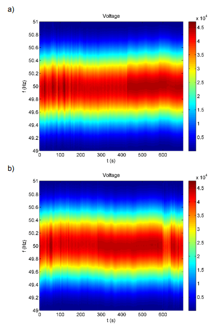
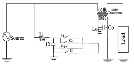
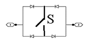
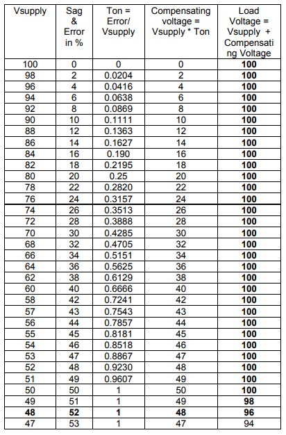
Voltage Fluctuations in Networks with Distributed Power Sources

Published by Maciej MRÓZ1, Zbigniew HANZELKA, Krzysztof CHMIELOWIEC2, TAURON Dystrybucja S.A.(1), AGH – University of Science and Technology (2)


Abstract. One of the electromagnetic disturbances generated by distributed power sources, e.g. wind turbines, are voltage fluctuations. An imprecise prediction of the disturbance level may be the reason for erroneous decisions made at the stage of issuing technical conditions of connection. In the authors’ opinion, the most common causes for errors can be: the lack of sufficiently precise tools for assessing the level of flicker attenuation, high uncertainty of prediction of the disturbance level after connection, and too low disturbance emission limits.

Streszczenie. Jednym z zaburzeń elektromagnetycznych emitowanych przez rozproszone źródła energii np. przez turbiny wiatrowe, są wahania napięcia. Brak precyzji w przewidywaniu poziomu tego zaburzenia po przyłączeniu źródła może być przyczyną błędnej decyzji na etapie wydawania warunków technicznych przyłączenia. Wśród wielu przyczyn błędu można wyróżnić zdaniem autorów brak wystarczająco precyzyjnych narzędzi dla oceny poziomu tłumienia wahań w sieci zasilającej, dużą niepewność prognozy poziomu zaburzenia po przyłączeniu źródła oraz przyjmowane zbyt niskie graniczne wartości miar liczbowych zaburzenia. Wahania napięć w sieciach z rozproszonymi źródłami energii

Keywords: flicker, propagation, transfer coefficient
Słowa kluczowe: wahania napięcia, propagacja, współczynnik przejścia

Introduction

Among many features of the smart grid technology at least two, related to the distributed generation, should be mentioned: the grid flexibility, understood as its capability for connection of a new power source and acceptance of a new and proven idea or technology, and the ability to supply sensitive loads or installations without degradation of their functionality. One of the electromagnetic disturbances generated by distributed power sources that in many cases can be an obstacle to their connection to the network are voltage fluctuations.

Power sources with power considerable large with respect to the short-circuit capacity at the point of connection may be sources of disturbances due to switching operations, e.g. starting or switching off, or continuous operation with variable output power. If power variations are slow they usually do not cause flicker. For instance, in the case of photovoltaic power sources, changes in solar irradiation as so slow that they do not cause flicker, whereas wind turbines, due to the nature of their operation, may cause flicker. Example of the impact of wind turbines on flicker level is presented in the figure 1.
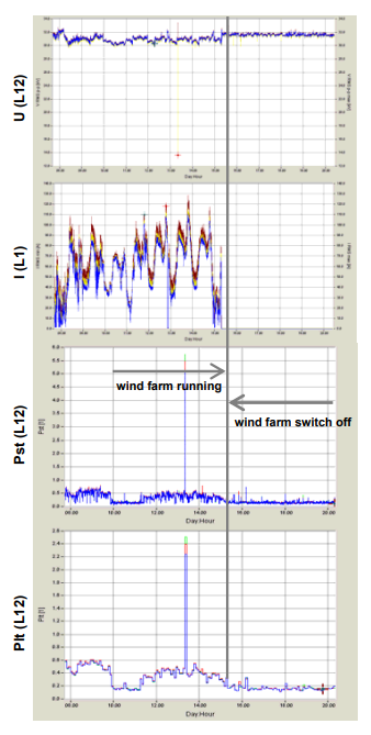
Fig.1. Voltage, current and flicker coefficient in wind turbine PCC

The possibility of precise prediction of the flicker level at the considered point of the network is of major importance at the stage of connecting new power source, e.g. a wind turbine or a wind farm. The lack of the precision in predicting may be the reason for erroneous decision concerning: acceptance of connection of a new source despite the actual, or possible future, high level of voltage fluctuation, or refusal of connection or limitation of a new source power.

Among many causes of erroneous prediction, the following should be mentioned:

a) difficulties in precise evaluation of the flicker attenuation effect in the existing network [3,4,8,11]. Measurements of voltage fluctuation are made at EHV/HV levels whereas their visual effects occur at LV. So the attenuation effect is essential.

b) the methods employed to estimate the disturbance level at the stage of connecting new sources are burdened with uncertainty [5]

c) in many cases there is a poor correlation between high flicker level and users’ complaints [1]. Rapid voltage changes or dip events that are not taken into account in planning procedures have a substantial share in the disturbance level [7].

d) modern energy-saving light sources have a lower sensitivity to voltage changes than traditional incandescent bulbs [1,2,6].

Factors (c) and (d) justify the thesis that present flicker levels limits are excessively stringent [1]. The above theses are further illustrated by simulation and experimental investigation.

Attenuation of voltage fluctuations

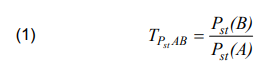
Voltage fluctuations generated at a given point of a network propagate across the power system disturbing even distant loads. The quantity that characterizes the system capability of disturbance propagation is the so called flicker transfer coefficient (TPst), which for two distant points – A and B, of the supply network can be defined as:
.

where: Pst(A)– flicker severity index at point (A), Pst(B)– flicker severity index at point (B).

A power system and loads connected to it have a capability to attenuate voltage fluctuations. This fact should be taken into consideration; otherwise it can be a source of costly errors. In literature are often expressed opinions that, in practice, voltage fluctuations are attenuated when they propagate towards a lower voltage network. It has been confirmed by multiple measurements (e.g. [1, 8]) that fluctuations generated in HV and EHV networks often become significantly reduced in MV and LV networks. So far there are no precise analytical methods to estimate transfer coefficients between networks at different voltage levels. Thus for estimated calculation are usually taken empirically determined values of transfer coefficients [5]: from EHV network to HV network ≈0.8; from HV network to MV network ≈0.9 (hence form EHV network to MV network ≈0.72); from MV network to LV network ≈1. Table 1 provides example values of transfer coefficients for given voltage levels. Estimation of flicker transfer coefficient with respect to statistical measures (Cumulative Probability CP95 and CP99) is possible only in the case of strong correlation between voltage fluctuations measured at points at different voltage levels.

Table 1. Example transfer coefficients [9]
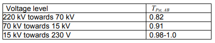
NOTE: Similar values apply to Plt index

The decision on voltage fluctuation planning levels for different voltages requires knowledge of transfer coefficients between given voltage levels. Moreover, flicker attenuation can also be of particular significance in the case of determining the voltage fluctuation emission limit for a given power source. According to the summation law [5,8] the global flicker level at the medium voltage busbars connected by the transformer to a high voltage network where the voltage fluctuation source is located, can be evaluated for the example exponent value m=3 from relation:

.

where: GPstMV – the global flicker level for medium voltage, LPstMV – the flicker planning level for medium voltage, TPstHM – the flicker attenuation coefficient between the high and medium voltage system, LPstHV – the actual flicker level at high voltage.

Assuming the voltage fluctuation planning level LPstMV=1.0 and LPstHV=0.8 in a medium voltage and high voltage network, respectively, and assuming the flicker transfer coefficient between the HV and MV network TPstHM=1, the total voltage fluctuation emission level in the MV network will be 0.6. Assuming the voltage fluctuation level 0.8 yields the total voltage fluctuation level 0.78 [8]. Not taking into account the flicker transfer coefficient between different voltage levels may lead to formulation of excessively stringent limits for connection of a fluctuating power source, e.g. a wind farm. Howerver, in the absence of certain knowledge, the effect of propagation of voltage flicker in the power system requires more real measurments and simulation studies.

Voltage fluctuations propagation between different voltage levels was investigated using a test network with nominal voltage 24.9 kV, connected through a HV/MV transformer to the 69 kV network. The test network model, based on IEEE 34 Test Feeder, is shown in figure 2.
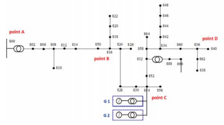
Fig.2. The test network model

The main source of voltage fluctuation utilized in the presented simulation are two wind turbines, 900 kW each, driven by variable mechanical torque from simulated wind speed. The variability of both: the voltage fluctuation level and its frequency, are achieved by changing the spectrum of turbines electromagnetic torque that simulate the variability of wind conditions. The voltage fluctuations are measured by means of a virtual flickermeter model. The measurement duration was 10 minutes for each transfer coefficient Pst value. Simulations were carried out in the ATPDraw environment.

Propagation of voltage fluctuations in the network with passive loads

Propagation of voltage fluctuation was simulated in a network containing solely the fluctuation sources (wind turbines) shown in figure 2. Short term flicker severity values obtained from the virtual flickermeter at selected points of the network model are shown in figure 2. The results indicate approximately constant voltage fluctuation level in the whole MV network. Differences between the indices values result from the magnitude of impedance between given measurement points.
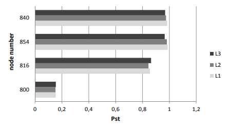
Fig.3. Short term flicker severity at selected points of the analysed network (Fig. 2)

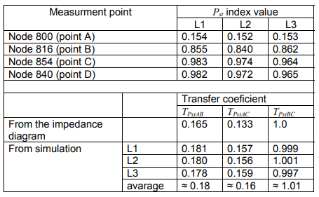
The test network has been loaded at different voltage levels (MV and LV) with passive balanced and unbalanced loads of total power ca. 3000 kW and average power factor 0.9. The computed flicker severity indices values at selected points of the network model are shown in Table 2.

Table 2. Flicker severity indices in network model
.

It is evident that due to the system large short-circuit capacity and the HV/MV transformer reactance, the voltage fluctuation level in the HV network (node 800) is relatively low compared to the voltage fluctuation level in the MV network. High flicker severity indices have been obtained at the network nodes closest to the voltage fluctuation source. The obtained results (voltage fluctuation level at node 890) confirm that there is practically no attenuation during the disturbance transfer from the medium to the low voltage network with dominant share of passive loads.

Transfer coefficients TPst between the given nodes are determined from the network impedance per-phase equivalent circuit, including connected loads. These values were compared with transfer coefficient values determined from the simulation, employing the network model and flickermeter model. Differences between transfer coefficient values determined from the per-phase impedance diagram and those determined from simulations are not exceeding 13%.

Equation (3) provides a simplified formula for determining the change in the transfer coefficient between the high and low voltage level depending on the HV/MV transformer percentage loading [11]:

.

where: PstMV – flicker severity index Pst at the MV transformer secondary side, PstHV – flicker severity index Pst at the HV transformer primary side, TPst(a) – assumed transfer coefficient for a transformer under no-load conditions.
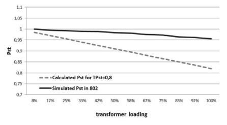
Fig.4. Short term flicker severity index at point 802 for different loading magnitudes of the test network. Solid line is based on simulation and dotted line shows calculated values assuming TPst=0,8

The dependence of the voltage fluctuation transfer coefficient versus the network loading level was simulated for the network in figure 2. The simulation results are presented in figure 4, which also shows the change in the transfer coefficient determined from relation (3) for the assumed value of TPst(a) = 0.8. The main inconvenience of the formula (3) is that the TPst(a) value needs to be assumed, which is not an easy task.

The linear relationship between the network (transformer) loading level and the voltage fluctuations degree has been confirmed. Nevertheless, assuming the voltage fluctuation transfer coefficient 0,8 between HV and MV for a network with exclusively passive loads can be a source of significant errors.

Propagation of voltage fluctuation in the network with passive and rotating loads

Both the actual measurements and theoretical analyses indicate that voltage fluctuations are attenuated during transfer between different voltage levels. As has been demonstrated in [14] the attenuation level depends mainly on the “dynamic”, not only on the static equivalent impedance of connected loads, chiefly rotating loads, i.e. electric motors directly connected to the network. The impact of rotating loads on the voltage fluctuation level was analysed in the configuration from figure 2. The source of fluctuation was, as formerly, two wind turbines and an additional fluctuation source in the HV network (Pst=0.85 at the node 800), added in order to increase the disturbance level. The network was loaded with passive loads (of total power about 3000 kW and power factor 0.9) and a varying number of motors with different rated powers, loaded with torques of various magnitude and type (constant or variable with the rotational speed square), connected at different nodes of the network.

The influence of the motor power on flicker attenuation

An induction motor of variable power, loaded with nominal torque was connected at node 816. The attenuation effect of the connected motor on the voltage fluctuation level is evident, and it increases with the motor power. Figure 5 illustrates changes in the severity index Pst at node 816 versus changes in the induction motor power within the interval 160 kW to 1500 kW, connected at the same point.

The share of rotating load in the network total loading increases with the motor rated power and therefore the effect of disturbance attenuation becomes stronger. Motors of lower rated powers can store smaller amounts of both: the mechanical and electromagnetic energy and, consequently, their capability to reduce the supply voltage fluctuation is limited.
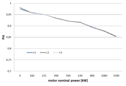
Fig.5. Flicker severity Pst characteristic at the point 816 vs. power of the induction motor connected at the point 816
The influence of motor location on the voltage fluctuation attenuation

Another investigated case was the influence of motor location on the voltage fluctuation level in the analysed network. For this purpose the simulation was carried out for induction motors with rated powers of 225, 500 and 800 kW under nominal load, connected at various points. The motors were successively connected at points: 848, 836 and 890. Flicker severity indices determined from the simulation are shown in figure 6 (average from values in three phases).

An alteration of the motor location only to a small extent influences the voltage fluctuation level. The observed effect will grow with the increase in the impedance values of the network sections between the selected points of connection, for which the parameters characterising voltage fluctuation have been determined.
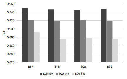
Fig.6. Flicker severity Pst at point 816 depending on the motor power and the point of its connection
The effect of the modulation frequency on the flicker attenuation level

The dependence of the flicker severity reduction versus the dominant voltage modulation frequency was also analysied – figure 7. For induction motors with different rated power, difference in the level of flicker severity reduction was observed in the low frequency range – up to 10 Hz. Reduction is less dependent on motors power rated, for higher modulatuion frequncy range.

Insecurity of voltage fluctuation prediction

A general empirical combination relationship for short-term flicker severity caused by several sources of emissions has the form formula (4):
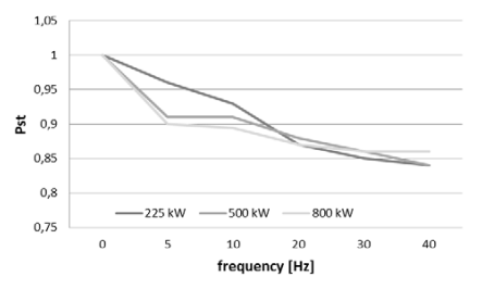
Fig.7. Flicker severity Pst characteristic at point 816 vs. the dominant voltage modulation frequency average from values in three phases

where: Pstj is the magnitude of flicker severity from various, independently operated, disturbance sources; exponent m is taken from 1 to 4, depending on the disturbance source characteristic.

In order to evaluate the correctness of prediction based on the relationship (4) were carried out simulations for the network in figure 2.

The influence of the wind turbine driving torque on the voltage fluctuation level

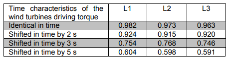
The simulation was carried out in two versions. First, the flicker severity indices were determined for the case of both wind turbines driven with same driving torque with time-characteristic shown in figure 8. In the second case the turbines’ driving torque time-characteristics were shifted in time. The results are provided in Table 3.
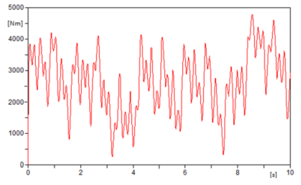
Fig.8. An example time-characteristic of the wind turbine driving torque

Figure 9 shows the flicker severity indices computed from the relationship (4) for different values of the exponent m. Also flicker severity indices obtained in the simulation for different, shifted in time, time characteristics of the wind turbines driving torque are shown (table 3). As can be seen, the relationship (4) is a highly imperfect tool for prediction of the voltage fluctuation level.

Table 3. The flicker severity factor P
.
Fig.9. Flicker severity indices in the analysed network

Influence of the frequency of voltage fluctuations emitted from different sources on the total disturbance level

The turbines in figure 2 were substituted by two hypothetical disturbance sources that modulate the voltage (i.e. its fundamental component 50 Hz) at the point of connection with the same modulation depth Vm/Vp=5% the relationship:

.

where: Vp – amplitude of the fundamental component, the modulated signal, Vm – amplitude of the modulating component, fb – the modulated signal fundamental frequency, fm – modulation frequency, Vm/Vp – modulation factor.

tor. The modulation frequency fm1 of one source was constant and equal 10 Hz whereas the other source modulation frequency fm2 was varied within the range of 0.5 Hz to 40 Hz. During the simulation this frequency was varied within a chosen interval. Flicker severity indices determined by simulation for given frequencies were compared to those found from the relationship (4) for different values of the exponent m. The results are shown in figure 10.

Once again it is evident that the relationship (4) is not enough perfect tool for prediction of voltage fluctuations. Depending on the exponent m value taken for calculations, the obtained total voltage fluctuation level was either overestimated or underestimated with respect to the simulation results taken as the reference.

Propagation of voltage fluctuations from a network with higher nominal voltage towards the network with lower nominal voltage

The voltage at the HV side, at point 800 was modulated by the sinusoidal signal with frequency fm=10 Hz and modulation depth 5%, that yields flicker severity level Pst=0.85 at the node 800. Loads with constant equivalent impedance were connected to the medium voltage network.
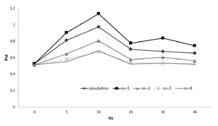
Fig.10. Comparison of the determined flicker severity indices

Short term flicker values Pst at the network selected points, shown in figure 11, confirm a very weak attenuation effect when only constant power loads were connected.

Additionally to constant impedance loads also induction motors with different rated powers loaded with constant nominal torque, were connected. The obtained flicker severity index values confirm former observations that only small part of the voltage fluctuations generated at the MV network propagate to a HV network (point 800 – figure 11). Also flicker severity indices obtained in the simulation shows that voltage fluctuations from different sources do not sum algebraically and cannot be simply added together, especially in cases where the source of fluctuations is connected to different voltage networks. The simulation
results are higher that obtained from the summation law (dotted line – figure 11).
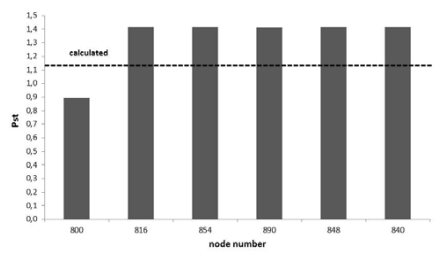
Fig.11. Short term flicker indices at the MW network selected nodes when the sources of fluctuation were connected to HV and MV network. Dotted line indicates flicker level obtained from relation (3)

Rapid voltage changes as a source of fluctuation

It happens that refusal of connection of a new power source, or limitation of a new installation power, results from the fact that measurements reveal to high level of voltage fluctuation in the existing network. Sometimes it is not caused by operation of distributed power sources but the effect of a large number of rapid voltage changes, voltage dips or swells. It is illustrated by the practical example below [7]. To test the effect of operating wind turbines on a supply network, the series of measurements at their connection points were carried out. The measurements were made at the nodes of a medium voltage network supplied from 110/15 kV GPZ. The scheme of the analysed network is shown in figure 12.

Over ten wind turbines were connected to the analysed medium voltage network either in groups as small farms or individually. The total installed power of wind sources at the investigated area is 2.85 MW. Short-circuit capacity at 110 kV level at GPZ is 1,480 MVA.
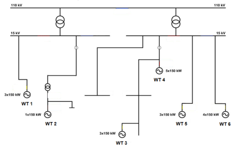
Fig.12. Scheme of analysed medium voltage network

The considered network is an overhead network and supply also the other consumers. Fig. 13 shows diagrams of the short term flicker severity factor Pst recorded on 15 kV busbars at the supply point. It is evident that the limits are significantly exceeded.

To find out a source of disturbances, the correlation between phase current of a farm, supply voltage and short term flicker severity factor Pst was investigated. It was found that large values of factors characterizing voltage fluctuations are caused by voltage changes and are not correlated with current changes. Figure 14 shows the correlation of wind farm phase current and the short term flicker severity factor Pst. Poor correlation of values confirms again that wind farms have no effect on a voltage fluctuation level in the analyzed network.
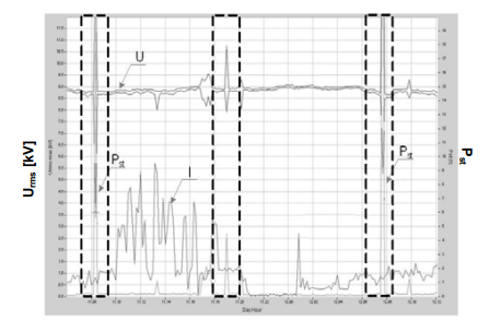
Fig. 13. Maximum values of current in relation to minimum and maximum values of voltages (av. 10 ms), and Pst, in the selected recording period

Considering the above indicated relations between the events on a voltage change characteristic and the factors characterizing voltage fluctuations, it was decided, in accordance with the standard EN 61000-4-30, to exclude the measured values of voltage fluctuation indicators recorded during voltage dips/swells. It was noticed that extreme voltages and large voltage fluctuation indicators occur simultaneously.
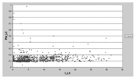
Fig. 14. Correlation of phase current and short term flicker severity factor Pst,


Table 4. The flicker severity factor Plt in analysed network

.

The samples Plt that contain the values Pst were excluded from statistical analysis. Such procedure of analysis was applied to particular measuring positions. As a result, the voltage fluctuations at connection points of wind farms to supply network were significantly reduced. The recorded and the assessed (after elimination of flagged samples) values of the long term flicker severity factor (Plt) are assembled in Table 4.

It is evident that the acceptance of the given procedure for excluding definite values of indicators characterizing voltage fluctuations reduced a voltage fluctuation level at particular points of supply network to allowable values. It is easily noticed that the number of events during particular measuring weeks was almost identical. That means that the events identified at various measuring positions were not connected with a limited area but with the whole analysed network.

Voltage fluctuation effect on energy-efficient light sources

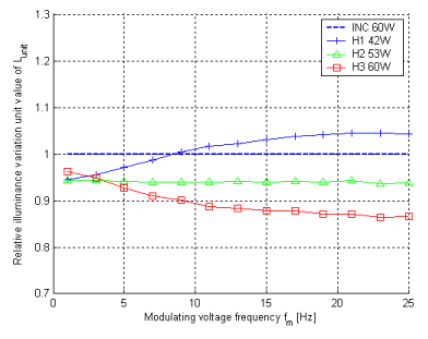
The lack of correlation between the flicker level, demonstrated by measurements, and customers’ complaints can also be explained by a lower sensitivity of energy-saving light sources to voltage changes. In almost all light sources, i.e. incandescent bulbs, fluorescent lamps, LEDs and CFLs, an increase in the modulation depth at constant frequency (0.5-25 Hz) increases the luminous flux variability (however to a different extent), whereas the same modulation depth at an increasing frequency does not always result in the luminous flux reduction. Incandescent light sources are almost linear loads, whereas the voltage-current characteristics of high-pressure discharge lamps and energy-efficient light sources are nonlinear. The voltage across a discharge lamp is an electronic converter output voltage and, therefore, it does not vary in accordance with the supply voltage changes.
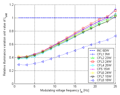
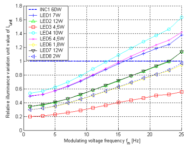
Fig. 15.1. Compact fluorescent lamp
Fig. 15.2. LED lamp
Fig. 15.3. Halogen lamp
Conclusions

The simulation results and measurements presented in this paper have confirmed:

1) Imperfection of tools commonly employed for prediction of flicker level resulting from connection of a fluctuating load. A large number of factors influencing the disturbance level is the cause that the only credible method for flicker level prediction is simulation. The forecast confidence depends fundamentally on the model accuracy degree.

2) In many cases the actual (measured) high level of voltage fluctuation results from voltage events, i.e. rapid voltage changes, voltage dips or swells that are not accounted for in simulation. That level does not influences directly costomers’ compalints. It seems that limit levels of the considered disturbance can be lowered, provided that attenuation has been accounted for and simulations will demonstrate that voltage fluctuation limit in LV networks is not exceeded. This will allow the network operator to approve multiple distributed power sources, as well as fluctuating loads that otherwise, according to binding regulations, would have no chance for connection. according to binding regulations, would have no chance for connection.

3) A further argument for liberalization of the existing regulations is the fact that frequency characteristics of energy efficient light sources are different from those of incandescent light sources.

This work was performed under the finance support of CIPOWER Project (KIC InnoEnergy).

REFERENCES

[1] Chmielowiec K., Flicker effect of different types of light sources, EPQU Conference 2011, Lisbon.
[2] De Jaeger E, Measurement and evaluation of the flicker emission level from a particular fluctuating load, Prepared for CIGRE/CIRED Joint Task Force C4.109, October 2007.
[3] Guide to quality of electrical supply for industrial installations. Part 5: Flicker, UIEPQ 1999
[4] Gutierrez J.J, Ruiz J., Azkarate I., Saiz P. Analysis of the sensitivity to flicker of the modern lamps, Group of Signal and Communications, University of the Basque Country, Report to WG2 of SC77A/IEC, London, September. 19, 2011.
[5] Hanzelka Z., Mroz M., Pawelek R., Piątek K Quality parameters of 15 kV supply voltage after connection of wind farms – case study, 12th International Conference on Harmonics & Quality of Power : 1–5 October 2006 Cascais, Portugal.
[6 IEC 1000-3-7: Electromagnetic compatibility (EMC) – Part 3: Limits – Section 7: Assessment of emission limits for fluctuating loads in MV and HV power systems – basic EMC publication.
[7] Povh D., Weinhold M. Improvement of power quality by power electronic equipment. CIGRE Session 2000, 13(14)36-06.
[8] Power quality indices and objectives, CIGRE WG C4.07, Oct. 2004.
[9] Tennakoon S., Perera S., Improvement of power quality by power electronic equipment. CIGRE Session 2000, 13(14)36-06.
[10] Yang X.: Kratz M., Improvement of power quality by power electronic equipment. CIGRE Session 2000, 13(14)36-06.
[11] Reviev of Flicker Objectives for LV, MV and HV System. CIGRE/CIRED WG C4.108
[12] Rogóż M., Quality assessment system for the electricity supply contract and determine the technical conditions of connection, Phd Thesis, AGH, Kraków 2007
[13] Lubosny Z., Wind Turbine Operation in Electric Power Systems; Springer-Verlag Berlin, 2010
[14] Tennakoon S Flicker propagation in radial and interconnected power system, Phd Thesis, University of Wollongong, 2008
[15] Halpin M., Cai R., De Jager E., Papic I., Perera S., Yang X., A revive of flicker objectives related to complaints measurements, and analysis techniques, 20th International Conference on Electricity Distribution CIRED 2009, Prague, Czech Republic.


Authors: mgr inż. Maciej Mróz, TAURON Dystrybucja S.A., ul. Jasnogrska 11, 31-358 Kraków, prof. dr hab. inż. Zbigniew Hanzelka, AGH – Akademia Górniczo – Hutnicza, Katedra Energoelektroniki i Automatyki Systemów Przetwarzania Energii , al. Mickiewicza 30, 30-059 Kraków, E-mail: hanzel@agh.edu.pl; mgr inż. Krzysztof Chmielowiec, Katedra Energoelektroniki i Automatyki Systemów Przetwarzania Energii , al. Mickiewicza 30, 30-059 Kraków, E-mail: kchmielo@agh.edu.pl.


Source & Publisher Item Identifier: PRZEGLĄD ELEKTROTECHNICZNY, ISSN 0033-2097, R. 90 NR 5/2014 228. doi:10.12915/pe.2014.05.50

Causes and Solutions of the Potential Induced Degradation (PID) Effect in PV Modules

Published by Pietro Tumino, EE Power – Technical Articles: Causes and Solutions of the Potential Induced Degradation (PID) Effect in PV Modules, July 09, 2020.


In case you are dealing with unexpected and unreasonable power loss in your photovoltaic plant, you may be experiencing the PID effect in the PV modules. 

Potential induced degradation (PID) is a phenomenon that arises over time (months or even years). It may be negligible in the plant’s early stage but, over time, becomes more noticeable in advanced phases, causing important power losses. However, it’s not always easy to determine the main cause. 

Where Does PID Occur in PV Modules?

PID is related to the negative potential that each PV module can deal with when working in normal operative conditions. PV modules are connected in series to create a string and the overall string voltage is distributed among all the single PV modules. How this voltage distribution happens depends on the inverter type used. 

For example in case of a 1000V DC system we can have the following simple classification: 

Transformerless inverter: Typically the voltage is distributed symmetrically -500V … + 500V but it depends on the inverter type because, in some cases, it’s common to have an offset more in the negative side (for example -700V … + 300 V).

Inverter with galvanic isolation: The voltage is distributed in a symmetrical way -500V…+500V.

Inverter with galvanic isolation with one pole grounded: In this case, the voltage distribution will be 0V…+1000V if the positive pole is grounded, or -1000V…0V if the negative pole is grounded.

In these voltage distributions, considering a 1000 V DC system, each PV module has about 50V of voltage across its terminals.

As said above, the PID effect is linked to the negative potential of each PV module, so the higher the negative voltage is in the overall voltage distribution, the higher the probability to experience this effect. Let’s focus on how it works actually. 

Potential Induced Degradation Explained

A PV module is made by several components (Figure 1), but the ones that play an important role in this discussion are the solar cell, the encapsulant material (EVA in most of the cases), and the aluminum frame. 

Figure 1. PV module composition. Image courtesy of PV Education.

When a solar cell is polarized with a high negative voltage, there is a relevant voltage difference between the cell itself and the module frame. This is at zero potential because most of the time it is grounded, so, due to the very short distance between solar cells and frame and due to possible presence of impurities in the encapsulant material, a current can be created between the cells and the frame, generating a current leakage for the entire PV module. 

Figure 2. Possible leakage current path. Image courtesy of Fraunhofer.

Let’s look at an example to better explain the effect. Suppose we have a transformerless inverter with symmetrical distribution at 1000V DC. 

The voltage distribution on the string will be like the one shown in Figure 3.

Figure 3. Example of voltage distribution in the string connected to a transformerless inverter at 1000V DC system.

The PV module that falls in the more negative section of the string will be the most affected by this effect because its cells would be polarized at around -500V while the frame of the module is at 0 potential (because it is grounded). So, there is a very high potential difference that can create a leakage current from the cells to the ground. Once the effect takes place, it becomes more evident with time and the leakage current will keep increasing. 

How to Detect PID in a PV Module

To determine if a PV module is affected by PID, it’s possible to perform an I-V curve test or an electroluminescence test. Note that the electroluminescence test only indicates if some cells are underperforming without giving any relevant indication about the causes.

The I-V curve test is more appropriate in this case due to the nature of the PID effect. PID reduces the performance of the PV modules due to a reduction in the shunt resistance of the electrical model (Figure 4). This corresponds to an increase in the leakage current, resulting in a decrease of the output current (and so, total output capacity) and affects the I-V curve as shown in Figure 5.

Figure 4. One-diode model of a PV module. Image courtesy of Sandia.
Figure 5. I-V curve comparison between PV module affected by PID and not affected by PID. Image recreated from Caroline Bedin.
Mitigation Actions

Luckily, in most cases, the PID effect is reversible. However, if it has existed for a prolonged time without measures taken to fix the problem, it will permanently affect the cells and the encapsulant intrinsic properties. 

If PID has taken place, it can be mitigated by grounding the negative DC pole on the inverter in order to avoid negative voltages on the strings. This works if the inverter allows this operation mode and all the proper design action associated with this choice is taken. 

PID can also be mitigated by using a so-called “anti-PID box” that is installed between the strings and the inverter. The anti-PID box reverses the potential applied by the inverter in order to polarize all of the PV modules that were affected by the negative voltage in the opposite way. These boxes work to avoid each string from keeping the same polarization for too much time in order to reduce the probability of PID and giving each module the possibility to “recover” the negative potential suffered. 

PID Prevention Actions

In the case of new PV plants, it’s important to focus attention on the type of materials and the design choice of each module before making any purchases. 

Design choices that can affect the occurrence of PID are mainly related to PV module choice. For example, choosing a frameless PV module reduces the probability of PID because the region at zero potential would be very minor compared to a frame module. Only a small portion of the clamps dimension will have ground potential. There will also be additional insulating material between the clamp and PV modules, so a possible leakage current would have less probability of appearing. 

On the other hand, frameless modules are typically double glass with a higher weight and they cost a bit more, so they’re not always the best choice for all projects. Generally, it’s possible to focus on the quality of the PV module and its bill of materials before purchasing. In this sense, the IEC standard provides support on the required quality. 

There is a specific standard family — IEC 62804 Photovoltaic (PV) modules: Test methods for the detection of potential-induced degradation — that aims to detect the potential induced degradation in the early life of PV modules by testing products under extreme conditions that represent an acceleration of the PV module lifetime. 

Once PV module manufacturers get their products certified for the IEC 62804 family, they usually add the label “PID free” to their product. Unfortunately, this label does not guarantee that PID won’t take place, and with the current technology, completely PID free modules don’t exist. Let’s have a look at the meaning of this certification to better understand why.

The test conditions to detect the potential induced degradation according to the IEC 62084 are:

• 60°C air temperature
• 85% relative humidity
• voltage biases of +1000 V, -1000 V, +1500 V, or -1500 V (according to the PV module characteristics)
• total test duration of 96 hours

The pass criteria are mainly related to the power degradation measured at the end of the test. If it does not exceed 5%, the test has been passed. So, the test does not ensure that PID won’t happen or that a module is PID free, it just measures the power degradation after operation under specific extreme conditions for a defined time period. 

However, it is possible to take results from the certification that each manufacturer can provide. PV modules with lower power degradation in the IEC 62804 certification would probably be the most resistant to the PID effect when compared to other PV modules with higher power degradation. It’s also worth saying that some manufacturers are starting to perform the certification with increased time duration (up to 600 hours) and a similar certification would be reliable for obtaining a product with strong resistance to the PID effect.


Author: Pietro Tumino received his MSEE from the University of Catania in March 2012. His great passion for renewable energies brought him to join Enel Green Power, where he has worked since November 2015, starting at Solar Centre of Excellence in the Solar Design unit/Engineering and now as Project Engineer. He focuses on the design of photovoltaic plants, planning and coordinating photovoltaic projects in the development and execution phases. Previously he worked at Enel Distribuzione, focusing on network technology unit/remote controls and automation systems and helping the development and testing of solutions for smart grids. In his downtime, he loves football, playing guitar, and rock music.


Source URL: https://eepower.com/technical-articles/causes-and-solutions-of-the-potential-induced-degradation-effect-in-pv-modules/

Resource-Saving Protection of Powerful Electric Motors

Published by Mark KLETSEL1, Abdulla KALTAYEV2, Bauyrzhan MASHRAPOV2,
National Research Tomsk Polytechnic University (1), Pavlodar State University (2)


Abstract.The article presents the disadvantages of traditional and some new electric protections of powerful electric motors. It is proposed to eliminate these drawbacks by constructing phase-sensitive protection that does not use current transformers, with a majority circuit and functional diagnostics. The methods of choosing protection settings are given. The algorithm of its functioning, implementation and operation in various modes is considered.The construction for mounting to protect the blocks near the conductors of the motor phases is presented.

Streszczenie. W artykule zaprezentowano mankamenty obecnie stosowanych metod zabezpieczania mocnych silników elektrycznych. Na tej podstawie zaproponowano nową fazoczułą metodę nie korzystająca z przekładników prądowych. Nowa metoda zabezpieczania silników elektrycznych ochraniająca środowisko

Keywords: phase comparison, parameters, operation, majority element, diagnostics, motor protection, magnetically-operated switch
Słowa kluczowe: zabezpieczanie silników elektrycznych, porównanie fazy

Topicality

Powerful electric motors (EM), including with heavy start conditions [1], are usually equipped with overcurrent and differential protection against short circuits [2, 3]. These protections have the following well-known disadvantages: do not reveal coiled-circuit in the stator winding and phase failure (which may cause a fire [4]), sometimes denied due to faults of elements that make up, and, in addition, require current transformers. The devices for early evidence of stator winding failure also require them [5]. Current transformers are metal-intensive (containing tens of kilograms of high-grade steel and copper) and may have unacceptable errors [6,7,8], because of which the differential protection is necessary to complicate significantly. There are proposals [2, 9, 10, 11] to reduce the impact of the errors on the basis of the phase comparison by building defenses. All these protections receive information via a current transformer, except for [11],and do not use special techniques, except for [10], to improve reliability. In this paper we propose a protection [12], which has the advantage of protection on [10] and [11] at the same time.

Protection device

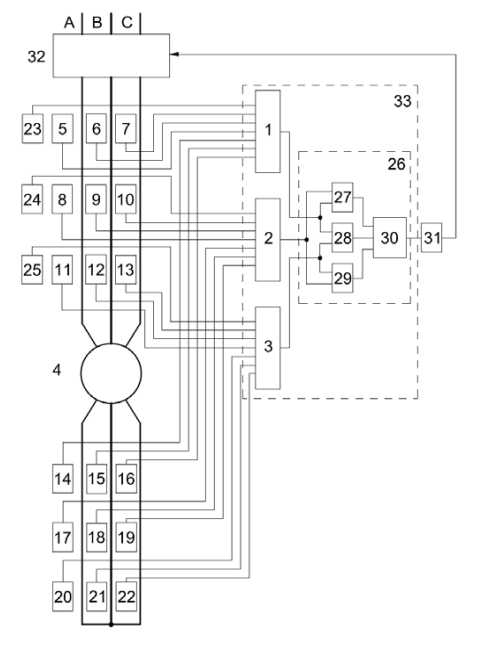
The majoritarian principle of construction “2 of 3” is being used. It is known, this arrangement increases the reliability of operation and failure of dozens of times. The protection consists of failure identification blocks 1, 2, 3, receiving information about the protected motor 4 and the supply cable from its blocks 5-25. Blocks 1, 2, 3 overlap each other as blocks 5, 6, 7; 8, 9, 10; 11, 12, 13; 14, 15, 16; 17, 18, 19; 20, 21, 22; 23, 24, 25.

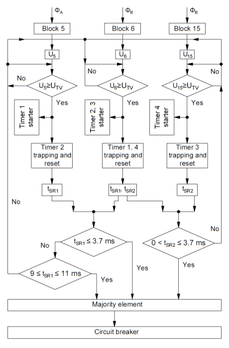
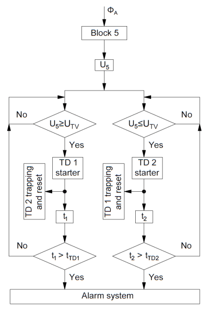
The blocks 5-22 contain two magnetically operated contacts (MC) with the same parameters, the blocks 23-25, one contact. Magnetically operated contacts have been selected when they are used in protective relaying, they have important advantages compared to other magnetically sensitive elements [13, 14, 15]. In this case the blocks 5-13, 23-25 are mounted on the supply side near the electric conductors 4 of phases A, B, C, and the blocks 14-22 from zero leads. The first-contact blocks 5-13, as well as the second-contact blocks 14-22, are triggered in the positive half-wave alternating current, and the second-contact blocks 5-13 and 14-22 first-contact blocks – in the negative. The triggering – this is the first touch of the mobile magnetic contacts of magnetically operated contacts with the fixed plate. It is triggered by a magnetic flux F generated motor phase current in one or the other half-wave of the alternating current. It is provided according to the method described in [16]. Tripping signals are transmitted in the blocks 1, 2, 3 and the connecting cables (as in the conventional traditional protections), and these blocks are fed to majority element 26 consisting of AND the blocks 27- 29 and OR the block 30. The element 26 sends a signal to the execution block 31, if there are signals from any two blocks determining damage. The block 31 gives a command to turn off the switch 32. The blocks 1, 2, 3, and the majority element 26 are a part of the microprocessor 33.The block diagram of the protection device operation algorithm is presented in Figure 2. It shows how to identify Coiled-circuit in phase A (B), phase to phase fault AB (BC) and phase failure C. The rest of the algorithm is easy to imagine on the basis of the analysis of Fig. 1 and 2.

Fig.1. Functional diagram of the protection device
Selection of parameters

It is known that in normal operation of the motor phase angle shift between the currents of 120°, and its interwinding fault is less than 60° (between damaged and undamaged phases) [2] by 180°.

With loss of one phase currents intact phases are shifted by 180°. If there is phase short-circuit in the motor, and in the supply of its cable, faulty phase currents from the power supply and from zero findings are shifted relative to each other by 120°-180° [2].In other modes, the shift between the currents is equal to 0°. Based on the above, assuming that the measurement error can reach 10%, as the operation parameters adopted: by turn-to-turn circuit time between operations of magnetically operated contacts of different phases tSR1≤3.7 ms (corresponds to 66°), in case of interruption phases – 9≤tSR1≤11 ms, for phase short circuits time between operations of magnetically operated contacts of one phase (from the input terminals, and zero) – 0≤tSR1≤3.7ms. In the latter case, it is taken 3.7 ms instead 6.6-10 ms (120°-180°), because the contacts magnetically controlling interphase circuit triggered in different half-wave alternating current in the normal mode tSR=10 ms. The level of current bus systems in motor phases at which controlled the angle between the phase currents (in fact it is a current of protection operation) must be at least by turn-to-turn circuit current IIA idling in “K” times, where K=(1.5-2) It corresponds to the coefficient of sensitivity of current protection. Otherwise, magnetically operated contacts do not work, because at turn-to-turn circuit during idling (in a load operation), the value in the current phase changes insignificantly [2]. Since the currents of idling motor make up (0.1-0.5) In, where In – rated motor current, the currents in such conventional magnetically operated contacts, produced in Russia, can be insensitive. The minimum induction in the magnetic field required for the operation of magnetic contacts, is determined by the following formula [17]:

.

where μ0 – permeability of air; γ – the angle between the vector of magnetic induction created by a conductor, and the longitudinal axis of the MC; ISR – the minimum value of the current in the conductor, in which the contact is triggered magnetically; FSR – magnetomotive force (m.m.s.) solenoid actuation contact; Lk – the length of the solenoid, in which magnetomotive force is measured; h – the distance between the center of gravity of the magnetic contacts and a conductor.

For example, the minimum m.m.s. FSR corresponding to the position of contact with the magnetically γ=0° and h=0.02 m, engine capacity of 2 MW with load current In=230 A current and idle IIA=46 A, is equal to 4.8 A. This value m.d.s. is not sufficient to trigger the very magnetically sensitive contact, manufactured in Russia, – ICA-14103, as its m.d.s. It is within 8-35 A. Sensitivity can be increased by about 8-9 times with a DC bias [13], or use a Japanese mercurymagnetically operated contacts, which is much more sensitive and more durable but more expensive.

Operation in the different modes in the absence of faults in it

When turn-to-turn circuit and loss of one phase of the motor 4 in the positive half-wave of the AC unit 1 receives signals from the first block of magnetically contacts 5-7.

For example, when turn-to-turn circuit in the phase A, or phase failure C, in blocks 5 and 6 are activated first magnetically operated contacts, and at the output of the voltage appearing U5 and U6 (Fig. 2), which are fed into the unit 1, which compares with a threshold UTV value. If the solenoid contact block 5(6) is activated earlier, U5≥UTV (U6≥UTV), and starts a TIMER 1(2). It counts the time until the solenoid has not yet triggered the contact block 6(5) as U6≥UTV (U5≥UTV), then TIMER 1(2) stops. Recorded time between operations of magnetically operated contact will be stored and compared with the adopted setpoint to detect interturn short circuits. If tSR1≤3.7 ms, the signal is in a majority element 26. If tSR1≥3.7 ms, the phase failure condition is tested, wherein 9≤tSR1≤11 ms. When the latter signal is also applied to an element 26 which runs the block 31, the switch 32 is switched off. Behaves similarly to the negative half-wave device AC when triggered magnetically contacts the second block 5 and 6. Similarly, as the blocks 5 and 6, the blocks 8 and 9 run, 11 and 12, and then the blocks 2 and 3, the signals from the last served in block 26.

Fig.2. Block diagram of the protection algorithm

If there is interphase short circuit inside the motor 4 or the cable connecting it to a switch 32, for example between phases A and B, the first magnetically operated contacts blocks 5(6) and the second magnetically operated contacts blocks 14(15) are activated in one half-wave alternating current, and the second magnetically operated contacts blocks 5(6) and the first magnetically operated contacts blocks 14(15) – in the other, and also, as described in the preceding paragraph, checked the condition of 0<tsr2≤3.7 ms.

To protect the motor 4 from the three-phase short circuit at the time of its inclusion blocks 23-25 are provided with magnetically operated contacts, detuned from the start-up currents.

Construction for mounting of blocks with magnetically operated contacts

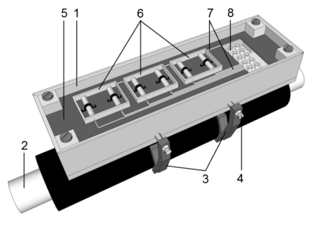
The installation of units with reed contacts 5-25 near the motor can be carried out using a special attachment construction, for example, [18] and shown in Figure 3.

The latter allows you to mount the blocks on each phase of the motor. The construction consists of a housing 1 with a cover, made in the form of a parallelepiped. The housing is secured to the current-carrying conductor 2 by means of guide units 3 and 4. The pins inside the housing obliquely positioned strip 5 with fixed parallel units with reed contacts 6. All units with reed contacts by means of connecting wires 7 are connected to the terminal block 8, to which connect the microprocessor and the source of the operational DC.

Fig.3. Construction for mounting blocks with magnetically operated contacts near the motor phases

Fig.3. Construction for mounting blocks with magnetically operated contacts near the motor phases: 1 – a body with cover (cover made of transparent material); 2 – busbar; 3 – rail links; 4 – pins; 5 – lath; 6 – blocks with magnetically operated contacts; 7 – connecting cables; 8 – terminal block

Failure diagnosing

The structural diagram of failure diagnosing algorithm is shown in figure 4.

By the of magnetically-operated switch fritting in the blocks 5-25, for instance, in block 5, a voltage is applied (Fig. 4) on the body of the first time delay (TD1) which controls the time t1 malfunction. If t1≥tTD1 (tTD1 – the time set in the TD1), then a fault signal will be emitted.

If there is no fault, then t1<0.01 s, because the magnetically-operated switch is activated and there is no contact within one halfwave of the alternating current by providing a polarity response [16]. Therefore, taking tTD1=0.02 s we can detect magnetically-operated switch fritting. If the wires are broken or if the unit is destroyed due to lack of voltage, the time delay starts second body (TD2), which controls the time t2 failure in the absence of the signal, and if t2≥tTD2 (tTD2 – time set on TD2), the signal is fault. When these faults occur in any circuit device of the considered motor or damage the cable, the signals from the undamaged blocks 8-13 and 17-25 come into blocks 2 and 3, which, in turn, provide signals to the element 26 and protection fires.

Conclusion

1. The considered method for determining the angle between the motor phase currents can detect phase to phase and Coiled-circuit.

2. The received construction gives an opportunity to save copper and steel to protect and preserve the working capacity at fault in any one of its units.

3. The proposed construction allows to strengthen the protection units to the cores of entrance motor cable.

Fig.4. The structural diagram of failure diagnosing algorithm

REFERENCES

[1] Jakub Bernatt, Silniki wysokiego napięcia dla trudnych warunków rozruchowych (projektowanie i wykonawstwo), Przeglad Elektrotechniczny, 2010, No. 8, 294-297
[2] Korogodskii V.I., Kuzhekov S.L., Paperno L.B., Relay protection of electric voltages above 1 kV, M.: Elektroatomizdat, 1987, 248
[3] Andreev V.A., Relay protection and automation of power systems: a textbook for high schools – 4 th ed. Revised. and additional, M.: Wysshaya. shkola, 2006. 639
[4] Andrzej Szczurek, Fires cause by electric reasons, Przeglad Elektrotechniczny, 2010, No. 9, 351
[5] Czesław Kowalski, Marcin Wolkiewicz, Paweł Ewert, Analysis of stator faults of the induction motor fed from net and static converter, Przeglad Elektrotechniczny, 2008, No. 12, 64-67
[6] Kuzhekov S.L., Nudelman G.S. About ways to reduce the errors of current transformers in transient influence on the work of relay protection of electric power systems, the International Scientific and Technical Conference of CIGRE: Modern directions of development of systems of relay protection and
automation of power systems, Moscow 7-10 September 2009, 99-104
[7] Xuesong Zhou, Zhihao Zhou, Youjie Ma, Dongfang Wu. Analysis of Excitation Current in DC-Biased Transformer by Wavelet Transform, Przeglad Elektrotechniczny, 2012, No. 05b, 108-112
[8] Waldemar Rebizant, Krzysztof Solak, The impact of current transformers saturation on operation of transmission lines protection relays, Przeglad Elektrotechniczny, 2010, No. 11a, 303-307
[9] A. Bogdan, Voronich I.A., Kletsel M.J., Nelyubin V.P., Differential-phase motor protection, Electric station, 1979, No. 2, 63-65
[10] Kletsel M.J., Musin V.V., Simonov S.N., Polyakov V.E. Protection of motors with phase-sensitive majority circuit and functional diagnosis, Electricity, 1990, No. 10, 27-32
[11] The innovative patent of the Republic of Kazakhstan 22073. The device to protect the motor from all kinds of stator winding circuits / Kletsel M. J. Publ. 18.12.2009. Bull. , No. 12.
[12] Patent of the Russian Federation No. 2570641. The device to protect the motor and its supply cable against short-circuit and phase failure / Kaltayev A.G., Kletsel M.J., Mashrapov B.E., Mashrapova G.N .Publ. 2014 Bull. , No. 34.
[13] Kletsel M.J., The principles of differential protection to the electrical reed switches, Electrical Engineering, 1991, No. 10, 47-50
[14] Kletsel M.J., Maishev P.N. Features of the construction of the differential-phase protections of transformers, Electrical Engineering, 2007, No. 12, 2-7
[15] Zhantlesova A.B., Kletsel M.J., Maishev P.N ., Neftis A.V. Identification of steady short-circuit current, Electrical Engineering, 2014, No. 4, 28-34
[16] Mark Kletsel, Nariman Kabdualiyev, Bauyrzhan Mashrapov, Alexander Neftissov Protection of busbar based on reed switches, Przeglad Elektrotechniczny, 2014, No. 1, 88-89
[17] Kletsel M.J., Musin V.V. On the construction of reed switches on the protection of high-voltage installations without current transformers, Electrical Engineering, 1987, No. 4, 11-13
[18] Patent of the USSR , No. 1767568. Measuring body for overcurrent / Dahno V.A., Kletsel M.J., Musin V.V., Metel’skii A.N., Alishev J.R. Publ. 07.10.1992. Bull. No. 37.


Authors: prof. doctor of technical sciences mr. Mark Kletsel, National Research Tomsk Polytechnic University, Tomsk, Russian Federation; mr. Abdulla Kaltayev, Pavlodar State University, Electroenergetics Faculty, Pavlodar, Lomov str., 64, Republic of Kazakhstan, E-mail: abdulla911@mail.ru; mr. Bauyrzhan Mashrapov, Pavlodar State University, Electroenergetics Faculty, Pavlodar, Lomov str., 64, Republic of Kazakhstan, E-mail: bokamashrapov@mail.ru.


Source & Publisher Item Identifier: PRZEGLĄD ELEKTROTECHNICZNY, ISSN 0033-2097, R. 93 NR 5/2017. doi:10.15199/48.2017.05.09

The New Design of the Vacuum Circuit Breaker Mounted on the Roof of Electric Traction Units

Published by Piotr BORKOWSKI1, Łukasz NOWAK1, Stanisław SZYMAŃSKI2,
Department of Electrical Apparatus of the Technical University of Lodz(1), Factory of Electrical Apparatus Woltan(2)


Abstract. This article presents the research on new design of a vacuum breaker type DCU-800M mounted on the roof of Electric Traction Units. The impact of one circuit breaker on another one was examined in detail when connecting them in parallel to the catenary.

Streszczenie. W artykule przedstawiono badania nowej konstrukcji wyłącznika próżniowego typu DCU-800M w wykonaniu dachowym. Szczegółowo sprawdzono wpływ jednego wyłącznika na drugi podczas podłączenia ich równolegle względem sieci trakcyjnej. (Nowa konstrukcja wyłącznika próżniowego montowanego na dachu Elektrycznych Zespołów Trakcyjnych).

Keywords: circuit-breaker, vacuum chamber, direct current, Electric Traction Units .
Słowa kluczowe: wyłącznik, komora próżniowa, prąd stały, Elektryczne Zespoły Trakcyjne.

Introduction

Vacuum DC breakers family type DCU-800M, generally used to secure traction against dangerous effects of short circuits and surge, has undergone modernisation. The aim of modernising was the production of a vacuum circuit breaker in the roof prepared for installation in new Electric Traction Units (ETU).

Vacuum circuit breakers produced by the Factory of Electrical Apparatus Woltan (FEA Woltan) licensed under the Department of Electrical Apparatus of the Technical University of Lodz (DEA of TUL) use the principle of turning off the short-circuit current by means of countercurrent, the source of which are capacitors. Turning off using the countercurrent method is equivalent to forced commutation of the current of the main circuit to the commutation circuit which consists of the pulse closing vacuum chamber [1-3] among others. Vacuum switches are designed to be used in circuits with a nominal voltage of 3 kV and catenary voltage variation from 0 to 4.5 kV. The effect of the carried out modernization was the creation of two independent vacuum breakers DC dedicated to the needs of producers in the new ETU. Circuit breaker DCU-800MNL was designed for the company NEWAG in Nowy Sącz while the circuit breaker DCU-800MNLD for the company PESA Bydgoszcz.

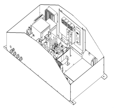
Fig.1. View circuit breaker DCU-800MNL after removing the top cover
DCU-800MNL

Vacuum circuit breaker DCU-800MNL (fig. 1) is a compact design inside which there is the main element (KG), which serves as a connector between the pantograph and the vehicle using the vacuum chamber (fig. 2). In turn, the auxiliary element (KP) is responsible for the inclusion of countercurrent during the shutdown whereas the second vehicle protection against short circuits is the element (ZF or ZPO). The source of countercurrent is the reactor (LK) and commutation capacitor (CK).The contact ssensor current (PIK) is responsible for the detection of short-circuit current. The energy needed to obtain high-speed traffic element (KG) is charged from the capacitors. The microprocessor control system, which uses fiber optics for the signal transmission, ensures the immunity of the electronic controls for distortion of the electromagnetic field.

The circuit breaker is equipped with a Harting connector, which acts as the main line system, via which communication between the switch and the vehicle takes place (the main driver of the drive system). Depending on your needs, we distinguish circuit breakers rated for control voltage 24 VDC, 110 VDC and special design 24/110 VDC.

Fig.2. Switch block diagram DCU-800M

Switch block diagram DCU-800M The applied microprocessor control system is equipped with a real-time clock and allows you, when you turn on the circuit breaker in the boarding pass CAN of the vehicle, to control the work validation of the circuit breaker on driver’s desk ETU and, in emergency situations, to determine the reason for not switching on of the circuit breaker or reason for its failure. Circuit breakers type DCU-800MNL are currently used by Regional Transportation for which the vehicles type IMPULSE were provided by the Polish company Newag in Nowy Sącz.

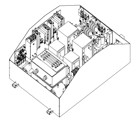
Fig.3. View of the circuit breaker DCU-800MNL after removing the top cover

DCU-800MNLD

Vacuum circuit breaker type DCU-800MNLD is a special version of type DCU-800MNL. Inside the cover there are two independently acting switches to ensure high factor readiness of the vehicle to operate (fig. 3). FEA Woltan produced the double configuration circuit breaker in a steel cover with dimensions 1800x1179x532 for the purposes of the ETU single. Due to the limited space and the imposed dimension of the cover, the kind offered by FEA Woltan is the only one introduced to active service in Poland.

When designing a circuit breaker in the double structure, the main idea was to create a product that guarantees reliability. Because the vacuum circuit breakers are modular, so in order to fulfill the customers’ needs FEA Woltan expanded the functionality of the circuit breaker by designing a common output for both vacuum breakers.

This solution resulted in parallel connection of circuit breakers to the catenary and the vehicle. Each circuit breaker is connected to the catenary by means of a separate pantograph (fig. 4). Depending on the direction of movement of the vehicle the first or the second circuit breaker is switched on. The introduction of a new configuration of the power circuit breaker ETU required the analysis of the technical parameters and carrying out additional tests for checking the correct operation of the circuit breaker DCU-800MNLD depending on the different configurations: circuit breakers (included/excluded) and pantographs (abandoned/raised).

Fig.4. Switch block diagram DCU-800M
Technical parameters

The technical parameters of vacuum circuit breakers of direct current type DCU-800M are unreachable for classic solution circuit breakers DC. If we assume nominal short-circuit conditions:

• rated operational voltage Ue = 3000 V,
• short-circuit expected Isp = 50 kA,
• time constant of circuit t = 20 ms,
• initial current rate of rise si = 2,5 A/μs,

for the above parameters the total break time of short-circuit currents by using the vacuum circuit breaker DCU-800M is not longer than 2.2 ms. The dynamics of the drive system guaranteeing the achievement of such a short time to open the DC circuit should ensure the full protection not only for the vehicle against the effects of short circuits in the catenary or circuits of the vehicle, but it should also fully secure the second connected in parallel circuit breaker. In order to verify the assumption a study to verify the declared time to open the DC circuit and voltage on the auxiliary chamber was conducted.

Testing the opening times of circuit breaker DCU800MNLD for a different configuration of power and (included/excluded) circuit breakers and the surge and voltage value on the auxiliary chamber.

Research of testing the opening times for a single circuit breaker and circuit breakers working in parallel was made in the Short-circuit Laboratory of Electrical Apparatus of the Technical University of Lodz. Measurements have confirmed a constant value of the opening time of the DC circuit regardless of the type of work.

A more important parameter of the work of the circuit breaker is the value of the voltage and its variability in the auxiliary chamber (in the countercurrent circuit) of the circuit breakers working parallel to the catenary. If we give the voltage 3 kV on the power terminals circuit breaker 1 and 1′ and then close the main chambers (KG), such circuit terms of the catenary together with closing any of the auxiliary chambers (KP) will be in a short time of around 200 ms short circuit.

Fig. 5. Diagram of research station
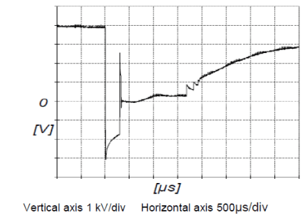
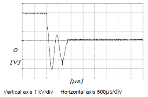
Fig.6. Oscillogram of voltage on the auxiliary chamber during the switch off of the circuit breaker 1 ‘

Voltage measurements on vacuum chambers (KP) were performed according to the measuring system shown in (fig. 5).

Measurements were taken in two modes during the process of a single-switch off and when the two circuit breakers were working in a parallel way. In the first place the voltage at the auxiliary chamber, voltage at the commutation capacitor and the supply voltage for the circuit breaker 1′ (individual work) were measured. Voltage oscillogram is shown in (fig. 6). The measured values of voltages are given in table 1.

Table 1. Measured characteristic Voltage

.

The second series of measurements were made by measuring the voltage on the auxiliary chamber of circuit breaker 1′ during the parallel operation (circuit breaker 1 turned on). Voltage oscillogram is shown in (fig. 7). The measured values of voltages are given in table 2.

Table 2. Measured characteristic Voltage

.
Fig.7. Oscillogram of voltage on the auxiliary chamber during switch off circuit breaker 1 ‘

Research shows that the voltage at the auxiliary chamber circuit breaker 1’ (fig. 6) varies depending on the process of shut-down. At the moment of opening of the contacts of the chamber (KG) voltage changes from the value of the 3950 V to the value of about -3000 V. After about 400 ms contacts of the auxiliary chamber close for 300 ms. Then, when you open the chamber the voltage between its contacts exponentially rises to the value of 3000 V. The difference of voltage before the closing of the chamber (KP) and it is reopening after the completion of the shut-down process equals 950 V.

In the second case, for the parallel operation of vacuum circuit breakers 1 and 1′ (fig. 7) the oscillating type of voltage in the auxiliary chamber (KP) was recorded, it lasted approximately 850 ms. This is the result of the flow of energy between the commutation capacitors of the circuit breaker 1 and 1′. The difference of voltage before the closing of the chamber (KP) and its reopening after the completion of the shut-down process equals 2850 V.

Oscillograms (fig. 6) (fig. 7) were recorded during the current less work of circuit breakers.

The confirmation of the correct work of the circuit breakers is a short-circuit test based on turning on both circuit breakers onto the compact power supply network. In the oscillogram (fig 8) voltage on the contacts of the auxiliary chamber circuit breaker 1′ was recorded. The measured values of voltages are given in table 3.

Table 3. Measured characteristic Voltage

.
Fig.8. Oscillogram of voltage on the auxiliary chamber during switch off circuit breaker 1

Contacts of the chamber (KP) remain closed for 400 ms, then the chamber is opened for 500 ms. From that moment the circuit breaker 1′ is opened. The further part of the course shows the effect of the closure of the auxiliary chamber circuit breaker 1 on the voltage waveform on the chamber (KP) of circuit breaker 1’. After the completion of the shut-down process the increase voltage on contacts chamber (KP) from the value of the 3950 V to 4200 V was registered. Voltage increase was caused by the flow of energy from a commutation capacitor circuit breaker 1 to the commutation capacitor circuit breaker 1′. During the test one observed the activation of both circuit breakers and signalling the exclusion of a short circuit.

Summary

During the parallel operation of two vacuum circuit breakers DC one found the interaction of one circuit breaker onto another. In the carried out, research circuit breaker 1′ switched off first, which led to, for a short circuit, breaker 1 switching off, too. These studies confirm the correct work of circuit breakers type DCU-800M in the case of detection of short circuits in the circuit. Parallel operation of two circuit breakers can be used when one wants to ensure the continuity of the drive system and auxiliary circuits of the ETU. It is ensured only when the vehicle is at a stop and one wants to change the steering cabin of the vehicle. If circuit breakers are working in parallel (redundantly) and one wants to switch off one of them, then, the high voltage circuit should be interrupted first by abandoning the pantograph and then sending a signal of switching off the circuit breaker. Otherwise, one will detect a short circuit and be turning off of both circuit breakers.

REFERENCES

[1] Bartosik M.,Wójcik F.,Lasota R.,Fast vacuum circuit breaker type of DCU-800 to shunting locomotives EM10, tts6 (2004), 36-37
[2] J. Magnusson, A. Bissal, G. Engdahl, J.A. Martinez-Velasco, “Design Aspects of a Medium Voltage Hybrid DC Breaker”, in 5th IEEE PES Innovative Smart Grid Technologies Europe (ISGT Europe), Istanbul, Turkey, 2014, pp. 1-6.
[3] A. Shukla, G.D. Demetriades, “A Survey on Hybrid CircuitBreaker Topologies”, IEEE Trans. Power Del., vol. 30, no. 2, 2015, pp. 627 – 641.
[4] Borkowski P., Błaszczyk H., The test protocol circuit breaker DCU-800MNLD, Łódź, 11.2017 r.
[5] Nowak Ł., Zaremba Ł., The test protocol with parallel operation circuit breakers used in the construction of DCU-800MNLD, Łódź, 06.2017 r.
[6] Zaremba Ł., Nowak Ł., Szymański S., Operation and Maintenance Manual ,,DC vacuum circuit breaker DCU-800M, DCU-800MNL, DCU-800MNLD’’, Łódź, 05.2017 r.


Authors: prof. dr hab. inż. Piotr Borkowski, Department of Electrical Apparatus of the Technical University of Lodz, ul. Stefanowskiego 18/22, 90-537 Łódź, E-mail: piotr.borkowski@p.lodz.pl;mgrinż. Łukasz Nowak, Department of Electrical Apparatus of the Technical University of Lodz, ul. Stefanowskiego 18/22, 90-537 Łódź, E-mail: Factory of Electrical Apparatus,,WOLTAN’’, ul. Gdańska 138, 90-536 Łódź, E-mail: Stanisław.szymanski@woltan.com.pl;


Source & Publisher Item Identifier: PRZEGLĄD ELEKTROTECHNICZNY, ISSN 0033-2097, R. 94 NR 8/2018. doi:10.15199/48.2018.08.32

Dissecting Electric Motor Malfunctions

Published by Alex Roderick, EE Power – Technical Articles: Dissecting Electric Motor Malfunctions, October 20, 2021.


Learn about the important electric motor parameters, such as voltage rating, acceleration time, overcycling, and insulation resistance, that should be taken into account to avoid electric motor malfunctions.

Electric motors are designed and sized to operate in HVAC systems for a number of years with minimal malfunctions or failures. For a motor to operate without malfunctions or failures, the motor electrical operating conditions must be within the original equipment manufacturer (OEM) operating specifications.

The motor operating specifications are listed on the motor nameplate. Motors are rated to operate at a specified voltage and current to deliver full horsepower without producing excessively high temperatures. In addition to the voltage being within the acceptable range of the nameplate rating, high transient voltages must be avoided because they can cause deterioration of motor insulation and electrical malfunctions.

Voltage Malfunctions

Electric motors have an operating voltage range in which they can perform satisfactorily. The OEM specifies the operating voltage range in the electrical specifications provided with the HVAC system or motor. It is standard practice to use the OEM specifications because the listed values are based on data from actual motor use and operating conditions. If OEM specifications are not available, the voltage range is normally +5% to –10% of the nameplate rated voltage (see Table 1).

Table 1. If original equipment manufacturer (OEM) specifications are not available, the motor operating voltage range is normally +5% to –10% of the nameplate rated voltage.

.

When measuring voltage, it is best to measure the voltage over time. A test instrument MIN MAX operating function can be used. Voltage measurements taken overtime should not vary by more than 3%. A high voltage fluctuation is an indication that the system is overloaded, the conductors connecting the system are too small, or the conductor run is too long.

For three-phase motors, the voltage between each of the power lines connected to the motor (T1 to T2, T2 to T3, and T1 to T3) should be measured. The voltage measured between any two lines should not vary more than 3%.

Excessive Heat Due to Motor Acceleration Time

When full power is applied to a motor, the motor accelerates to full speed. When a motor starter is used to start a motor, the motor must accelerate to its rated speed within a limited time period. The longer the time it takes the motor to accelerate, the higher the temperature rises in the motor. The greater the load under which a motor must operate, the longer the acceleration time. The maximum suggested acceleration time is determined by the size of the motor frame. Heat is dissipated faster by large motor frames than by small motor frames.

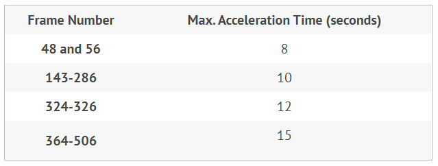
When a motor drive is used to control a motor, acceleration and deceleration time can be programmed to best match the requirements of the application. The programmed acceleration and deceleration time must not overheat the motor. Motor drives automatically control the voltage applied to a motor to keep it from overheating at all speeds. However, in HVAC systems, the motor acceleration time should be as short as possible. Normally, the OEM default settings for acceleration and deceleration times are acceptable (see Table 2).

Table 2. In HVAC systems, motor acceleration time should be as short as possible.

Maximum Acceleration Time – Magnetic Motor Starter

.

Maximum Acceleration Time – Magnetic Motor Starter

.
Overcycling

Overcycling is the procedure of repeatedly turning a motor on and off. Overcycling occurs when a motor is at its operating temperature and continues to cycle on and off. Starting current is several times the running full-load current (FLC) of the motor. Regardless if a motor is started using a motor starter or motor drive, most motors are not designed to start more than 10 times per hour because it increases the temperature of the motor, which destroys the motor wire insulation.

Overcycling in HVAC units occurs when the controlling temperature switch (thermostat) differential is set too low. The differential is the difference between the temperature at which a switch turns on a unit and the temperature at which it turns off the unit. For example, a 1°F differential keeps the temperature in a room within 1°F but requires the unit to continuously cycle on and off. Thermostats have a typical default differential setting of approximately 6°F (4.5°C).

When a motor application needs a motor to be cycled frequently, the following guidelines should be applied:

• Install a motor that has a 122°F (50°C) ambient temperature rating rather than a standard 104°F (40°C) rating.
• Install a motor with a service factor of 1.25 or 1.35 rather than a service factor of 1.00 or 1.15.
• Provide extra cooling by forcing air over the motor.
• Install a motor drive to control the motor so the motor speed can be controlled instead of cycling the motor fully on and off.

Note: The National Electrical Manufacturers Association (NEMA) standard MG1 sets the basic requirements for information to be marked on electric motor nameplates.

Motor Insulation Failure

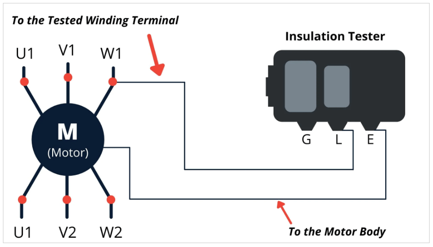
An ohmmeter is a test instrument that measures resistance. A megohmmeter is a high-resistance ohmmeter used to measure insulation deterioration on conductors by measuring high resistance values using high-voltage test conditions. A megohmmeter can detect motor insulation deterioration before a motor fails. Typical test voltages range from 50 V to 5000 V. A megohmmeter is used to measure the condition of motor wiring by detecting insulation failure caused by excessive moisture, dirt, heat, cold, corrosive vapors, or solids, vibration, and aging (see figure 1).

Figure 1. A megohmmeter is used to perform tests on motor insulation.

A megohmmeter is used to measure the resistance of different motor windings or the resistance from a motor winding to the ground. Several test measurements should be taken and recorded over time to provide a complete analysis of the insulation condition. The minimum acceptable insulation resistance depends on the motor voltage rating (table 3).

Table 3. The minimum acceptable insulation resistance of an electric motor depends on the motor voltage rating.

.

Note: A motor with good insulation may have readings 10 times to 100 times the minimum acceptable resistance. Service the motor if the resistance reading is less than the minimum value.

Cautionary Note: A megohmmeter uses high voltage for testing (up to 5000V). Avoid touching the meter that leads to the motor frame. Always follow the OEM recommended service and safety procedures. After performing insulation test measurements, connect the motor windings to the ground through a 5 kΩ, 5 W resistor. The motor winding must be connected to the ground for 10 times the motor testing time in order to discharge the energy stored in the wiring.


Author: Alex earned a master’s degree in electrical engineering with major emphasis in Power Systems from California State University, Sacramento, USA, with distinction. He is a seasoned Power Systems expert specializing in system protection, wide-area monitoring, and system stability. Currently, he is working as a Senior Electrical Engineer at a leading power transmission company.


Source URL: https://eepower.com/technical-articles/dissecting-electric-motor-malfunctions/

Monitoring of Electric Arc Furnace Supply Voltage Frequency using Phasor Analysis

Published by Szymon BARCZENTEWICZ, Krzysztof DUDA, Andrzej BIEŃ, AGH University of Science and Technology


Abstract. This paper presents the results of measurement experiment conducted in the operating steel plant. Frequency analysis of measured signals revealed an interesting phenomenon, as it happened that after switching off the electric arc furnace, the frequency of the supplying voltage and current increased slightly instead of decreasing, as we would normally expect. This abnormal frequency behaviour was identified by phasor analysis and also confirmed by the DTFT (Discrete Time Fourier Transform) analysis, and the MatrixPencil analysis.

Streszczenie. Artykuł prezentuje wyniki eksperymentu wykonanego w hucie stali. Analiza częstotliwości ujawniła ciekawe zjawisko, w którym po wyłączeniu pieca łukowego częstotliwości napięcia i prądu w wewnętrznej części huty zmniejszyła się zamiast zwiększyć, jak można by się spodziewać. To nieoczekiwane zjawisko zostało zarejestrowane z pomocą PMU i potwierdzone przez transformację Fouriera dla sygnałów dyskretnych oraz analizę MatrixPencil. (Monitorowanie częstotliwości napięcia zasilającego piec łukowy z wykorzystaniem analizy fazorowej)

Keywords: Electric Arc Furnace, frequency analysis, phasor analysis.
Słowa kluczowe: Piec łukowy, analiza częstotliwości, synchrofazor

Introduction

The electric arc furnaces (EAF) produce currents and voltages at the point of common coupling (PCC) with spectra reach in different types of disturbances. Those disturbances can cause power quality problems at PCC. Recently, researchers dealing with EAF are focused on harmonics and interharmonics analysis and methods of their mitigation [3,4]. This work is focused on the monitoring of frequency. The most popular nonparametric methods used for frequency calculation are based on the Fourier transform (FT). In this paper phasor based analysis is applied. There is a numerous group of phasor estimation methods. In this application FIR filters compliant with synchrophasor standard is used [3]. Phasor analysis is a well-established technology in transmission systems. Initially Phasor Measurement Units (PMUs) where considered as an expensive and highly specialized equipment, but lately, PMU tends to be less expensive and more popular. Moreover, DPMUs (PMUs for distribution systems) and phasor based frequency monitoring instrumentation were introduced. Authors propose a novel application of phasor analysis for the EAF frequency monitoring. Performed measurements revealed an interesting phenomena: after switching off the EAF the frequency of the supplying voltage and current increases slightly instead of decreasing, as we would normally expect. Recorded phenomenon was also confirmed by the Discrete Time Fourier Transform (DTFT) analysis [9], and the MatrixPencil analysis [10].

Phasor definition

Synchrophasors are measured with PMUs located across the network. Phasor data are collected in real-time and are accurately time-tagged. Synchrophasor is a phasor representation of sinusoidal signal. For the following continuous time sinusoidal signal

.

where: ω0=2πf0 is a nominal pulsation in rad/s, f0 is a nominal frequency in Hz, a(t) is time-vairing amplitude and φ(t) is a time-varying phase in radians, the phasor is defined as [7]

.

Equations (1) and (2) are related by

.

For the nominal frequency f0 = 50 Hz system, the phasor should be estimated 10, 25 or 50 times per second.

The instantaneous frequency fin of (1) is the 1st order time derivative of cosine argument in (1):

.

If fin ≠ f0, the phasor rotates on the complex plane.

The discrete-time x[n] corresponding to continuous time counterpart (1) is obtained by anti-aliasing analog LP filtering and sampling by an ADC converter

.

where Ω0 is normalized frequency (pulsation) in radians of the discrete-time signal, and n=-N,…,0,…,N is the sample index.

The instantaneous frequency of signal (1) is estimated as

.
FIR filters based on flat-top windows

Flat-top (FT) windows have an unique feature of simultaneous perfectly flat or equiripple spectral main lobe and fast decaying of the sidelobes. FT windows are cosine windows defined as [3]

.

where M is the window order and aM[m] are the coefficients of an M-order window. The window (9) has L=2N+1 samples. . It is shown in [3] that phasor estimation based on the FT window is compliant with the IEEE C37.118.1 in the M class.

Steel mill power supply

Steel plant is supplied with 400 kV voltage through 250 MVA voltage transformer. Plant consists of two pairs of arc furnaces and ladle furnaces. Both pairs are 500 meters apart and have separate power supply lines. Apparent power of first pair is 115 MVA and 75 MVA for arc furnace and ladle furnace respectively. Second pair is 25 MVA for both arc furnace and ladle furnace. Power supply network schematic is presented in figure 1.

Fig.1. Power supply network.

High power arc furnace is powered through two 75 MVA voltage transformers from 110 kV bus. Working in parallel transformers are the same type and production but it is expected that they are loaded differently. Measurements where conducted in three different points for high power arc furnace. Measurement point 1 and measurement point 2 ware installed on 110 kV side and Measurement point 3 on 30 kV side. The selection of these measurement points was dictated by the willingness to evaluate the impact of arc furnace A on PCC and attenuation of disturbances by transformers Tr1 and Tr2.

Measurement system

Measurement system is based on real time system with Field Programmable Gate Array (FPGA) module cRIO9024. It is designed for monitoring and control purposes. It allows to install eight different measurement, digital or control modules. Existing on site voltage and current transformers where used as a source of measured signals. The used configuration included three current measurement and three voltage measurement modules. Measurement signals are. Resolution of ADCs where 24 bits and maximal sampling frequency was 50 kS/s. Sampling was conducted with 12.5 kS/s frequency.

At each point, measurements of instantaneous values of three voltages and three currents were made. All performed measurements where conducted synchronously, according to one of the modules oscillator clock. Data after acquisition where send through FIFO queue with direct memory access (DMA) to real time system. Data was saved in a parallel thread on embedded data storage or on external Flash drive. Fig. 2 shows simplified block diagram of used data acquisition system.

Fig.2. Measurement system block diagram.

Results

Before computing phasors, signals were downsampled to the sampling frequency 800 Hz, and the phasors were computed, in respect to 50 Hz nominal frequency, as recommended in [1] with the flat-top window M=5, D0=2, DN=2, L=207 [2]. Fig. 3 shows the envelope of three phase voltages and currents obtained from phasors. In both cases, Fig. 3a,b, significant drop of current and slight increase of voltage is observed after switch off. In Fig. 3 time intervals t1 and t2, before and after electric arc furnace switching, are marked. Fig 4 shows instantaneous frequency computed by phasor and also the instantaneous frequency averaged with Finite Impulse Response (FIR) filter having flat impulse response. The arithmetic average was computed from 301 values. In Figs. 4 it is seen that the frequency change is different for case “a)” and “b)” although in both cases the electric arc furnace is switched off. In case “b)” the frequency unexpectedly decreases.

Fig. 3. Phasor envelopes of the three phase voltages and currents during the electric arc furnace switch off. For the case b) the decrease of supplying power system frequency after the switch off was observed, as further illustrated.
Fig.4. Phasor frequencies for the cases shown in Fig. 1.
Fig.5. Comparison of the instantaneous frequency estimated by phasor, DTFT and MatrixPencil for the cases shown in Fig. 1.

The results obtained by phasors are verified and confirmed with original, i.e. not downsampled, data with the DTFT (Discrete Time Fourier Transform) [5], the Matrix pencil algorithm [6-8], and the Interpolated Discrete Fourier Transform (IpDFT) [9]. Fig. 5 compares averaged instantaneous frequency computed by phasor with the Matrix pencil algorithm used as described in [7, 8] and the DTFT, both applied to signal in non-overlapping time windows of length equal to 100 periods of nominal frequency, i.e. 2 s. For the DTFT Hamming window was used and frequency step equal 0.001 Hz was set. The results of all three methods are in good agreement confirming observed phenomenon.

Fig.6. The DTFT voltage spectra for the cases shown in Fig. 1. For the red line the DTFT is computed in the interval t1 (Fig. 1), and for the blue line the DTFT is computed in the interval t2 (Fig. 2)

.
Fig.7. The DTFT current spectra for the cases shown in Fig. 1. For the red line the DTFT is computed in the interval t1 (Fig. 1), and for the blue line the DTFT is computed in the interval t2 (Fig. 2).

Fig. 8. Time-frequency voltage plots for the cases shown in Fig. 1; spectra computed by the DTFT with the Hamming window with length 2s without overlapping; frequency step equals 0.001 Hz.

Especially, abnormal frequency behavior in Fig. 7b is easy to be observed. Figs. 7ab show the DTFT of three phase voltage and current computed in time intervals t1 and t2 (see Fig. 3). The frequency of signals in intervals t1 and t2 was estimated by the three points IpDFT with the Hann window presented in [9], i.e. for α=2. The mean frequency in all measurement points for time intervals t1 and t2 is 49.973 Hz and 50.004 Hz for the case “a” and 50.023 Hz and 49.992 Hz for the case “b)”.

Fig. 8 depicts time-frequency voltage plots computed by DTFT with Hamming window with length 2s without overlapping with frequency step equal to 0.001 Hz.

Conclusion

The paper presents the results of spectral analysis of voltage and current signals supplying working arc furnace in industrial plant. It turned out that phasor measurements, based on computationally efficient FIR filter, can be used for spectral analysis in industrial plants, as confirmed by other more sophisticated and more computationally demanding frequency analysis methods.

REFERENCES

[1] Uz-Logoglu E., Salor O., Ermis M.: Online Characterization of Interharmonics and Harmonics of AC Electric Arc Furnaces by Multiple Synchrounous Reference Frame Analysis, IEEE Transactions on Industry Applications, vol. 52 no. 3, 2016, s. 2673–2683.
[2] Vatankulu Y. E., Şentürk Z., Salor O.: Harmonics and Interharmonics Analysis of Electrical Arc Furnaces Based on Spectral Model Optimization With High-Resolution Windowing, IEEE Transactions on Industry Applications, vol. 52 no. 3, 2016, s. 2673–2683.
[3] Duda K., Zieliński T. P.: FIR filters compliant with the IEEE standard for M class PMU, Metrology and Measurement Systems, vol. 23 no. 4, pp. 623–636, 2016
[4] Synchrophasor Measurements for Power Systems, IEEE Standard C37.118.1, Dec. 2011.
[5] Synchrophasor Measurements for Power Systems-Amendment 1: Modification of Selected Performance Requirements, IEEE Standard C37.118.1a, Apr. 2014.
[6] Duda K., Zieliński T. P., Barczentewicz Sz., Perfectly flat-top and equiripple flat-top cosine Windows, IEEE Transactions on Instrumentation and Measurement, vol. 65 iss. 7, 2016, s. 1558–1567.
[7] Hua Y., Sarkar T.K.: Matrix pencil method for estimating parameters of exponentially damped/undamped sinusoid in noise, IEEE Trans. Acoustics. Speech Signal Processing, vol. 38, no 5, s. 814–824,.
[8] Oppenheim A. V., Schafer R. W., Buck J. R.: Discrete-Time Signal Processing, 2nd ed. Englewood Cliffs, NJ, USA: Prentice-Hall, 1999.
[9] Zieliński T. P., Duda K.: Frequency and damping estimation methods – an overview, Metrology and Measurement Systems, vol. 18, no. 4, 2011, s. 505–528.
[10] Duda K., Zieliński T. P.: Efficacy of the frequency and damping estimation of a real-value sinusoid, IEEE Instrumentation & Measurement Magazine, vol. 16, iss. 2, 2013, s. 48–58.


Authors: dr inż. Szymon Barczentewicz, AGH University of Science and Technology, E-mail: barczent@agh.edu.pl, al. Mickiewicza 30, 30-059 Kraków; dr hab. inż. Krzysztof Duda prof. AGH, AGH University of Science and Technology, al. Mickiewicza 30, 30-059 Kraków, E-mail: kduda@agh.edu.pl; dr hab. inż. Andrzej Bień prof AGH, AGH University of Science and Technology, al. Mickiewicza 30, 30-059 Kraków, E-mail: abien@agh.edu.pl;


Source & Publisher Item Identifier: PRZEGLĄD ELEKTROTECHNICZNY, ISSN 0033-2097, R. 96 NR 5/2020. doi:10.15199/48.2020.05.10

Highest Voltage Sag and Swell Compensation using Single Phase Matrix Converter with Four Controlled Switches

Published by S. Abdul Rahman1, Shumye Birhan Mule2, Estifanos Dagnew Mitiku3, Gebrie Teshome Aduye4, C. Gopinath5, Department of Electrical & Computer Engineering, Institute of Technology, University of Gondar, Ethiopia (1, 2, 3, 4) Department of Electrical & Electronics Engineering, Sri Venkateswara College of Engineering, Chennai, India (5)


Abstract: The aim of this paper is to explain the control algorithm very clearly and precisely to achieve maximum voltage sag compensation of 52% and infinite quantity of voltage swell using direct converter based DVR. The proposed DVR topology has a single phase matrix converter (SPMC), series transformer and LC filter. If the duty cycle of the PWM is digitally computed by measuring the available voltage at the supply and the percentage of voltage sag, it is possible to mitigate 52% of voltage sag and infinite quantity of voltage swell with the THD less than 1%. Matlab Simulation results are presented for validating the analysis.

Streszczenie: Celem artykułu jest precyzyjne wyjaśnienie algorytmu sterowania w celu uzyskania maksymalnej kompensacji zapadu napięcia wynoszącej 52% i wzrostu napięcia przy użyciu rejestratora DVR z bezpośrednim przetwornikiem. Proponowana topologia DVR ma jednofazowy konwerter macierzy (SPMC), transformator szeregowy i filtr LC. Jeżeli cykl pracy PWM jest obliczany cyfrowo poprzez pomiar dostępnego napięcia na zasilaniu i procentu zapadu napięcia, możliwe jest złagodzenie 52% zapadu napięcia i wielkości wzrostu napięcia przy THD mniejszym niż 1%. Wyniki Matlab Simulation są prezentowane w celu walidacji analizy. (Kompensacja zapadów i wzrostu napięcie przy wykorzystaniu jednofazowego przekształtnika macierzowego z czterema przełącznikami)

Keywords: Voltage Sag, Voltage Swell, Single Phase Matrix Converter, DVR, Series Transformer, Digital PWM technique.
Słowa kluczowe: zapad napięcia, wzrost napięcia, jednofazowy przetwornik matrycowy, DVR, transformator szeregowy, ctechnika PWM

Introduction

Though we have many power quality issues like voltage sag, voltage swell, flicker, harmonics, etc., voltage sag is considered to be the severe issue as it affects the operation of sensitive loads like computer, micro controller, Digital Signal Processor, FPGA. As most of the industries are automated, the entire operation of the industries depends upon the operating condition of these embedded systems and sensitive loads. When sag or swell occurs in the industrial areas, these sensitive loads are getting affected, leading to immoral operation of the entire industry [1, 2]. For the compensation of voltage sag, Dynamic Voltage Restorer (DVR) considered to be an effective device when compared to other devices like UPS, STATCOM [3-5].

DVR is a series compensator, which is used to add the compensating voltage in series with the line voltage in order to mitigate voltage sag, swell, harmonics, flicker, etc. A conventional DVR has an energy storage device ( which may be a battery bank or capacitor or super capacitor), an inverter to convert the DC power in the energy storage device to AC power and a series transformer to inject the AC power generated by the inverter, in series with the line voltage. When a power quality issue occurs on the supply side, the inverter synthesis the required compensating voltage by taking power from the energy storage devices and injects the compensating voltage in series with the line voltage using the series transformer [6-8]. The compensating range and duration of mitigation of voltage sag and swell, of this topology is based on the rating of the energy storage devices. This conventional DVR has disadvantages like heavy weight, volume, uneconomical, more maintenance due to the energy storage devices [9- 11]. In order to overcome, these disadvantages, recently DVRs based on direct converters are proposed. In this topology, the energy storage devices are not used. Instead the power is taken from the supply side itself to mitigate the power quality issues. As the power is taken form the supply side to mitigate the power quality issues, this topology uses direct converters to synthesis the compensating voltage. A series transformer is used to inject the output voltage of the direct converter, in series with the line voltage. So when a voltage sag or swell occurs, the direct converter will synthesis the required compensating voltage by taking power from the supply side and the compensating voltage is added in series with the line voltage using the series transformer . As this topology didn’t used energy storage devices, it is not having disadvantages like topology based on energy storage devices. The compensating range and the mitigating duration of this topology is based upon the direct converter topology, modulating techniques and the availability of input voltage for the direct converter [12-16].

In the literature, very few publications are available for the DVRs based on the direct converters as it is recent technique. Out of those publications, the topology presented in [17] can mitigate 50% of voltage sag and 100% of swell by taking power from the same phase. The topologies presented in [18, 19] can mitigate 33% of voltage sag and 100% of voltage swell by taking power form the different phases. Though the topologies in [20-22] are based on direct converters, they can mitigate voltage sag, swell and also single outage. Based on the modulating techniques, the voltage sag and swell compensating range could be improved [23, 24]. In this paper, the DVR is realized using a Single Phase Matrix Converter (SPMC), which is a direct converter. The single phase matrix converter is realized using only four controlled switches but so far the single matrix converter is been realized using 8 controlled switches. As it is realized with 4 controlled switches, the generation of PWM pulses are very easy while compared to generation of switching pulses for 8 controlled switches. With the presence of 8 switches, the commutation problem occurs. But with 4 controlled switches, no commutation problems occurs as there is one bidirectional switch for each phase. In this paper, the achievement of 52% voltage sag compensation is clearly explained in a detail manner.

It is observed from the analysis that to mitigate voltage sag and swell by taking power from the same phase, using a DVR based on direct converter, by ordinary PWM technique, it is possible to achieve only 22% of sag and swell compensation. If the duty cycle of the PWM is digitally computed by measuring the available voltage at the supply side and the percentage of voltage sag, it is possible to mitigate 52% of voltage sag and infinite quantity of voltage swell with the THD less than 1%.

Principle of operation

The topology of DVR is been shown in the figure 1. It has a single phase matrix converter, a LC filters at the input side of the single phase matrix converter and another LC filter at the output side of the single phase matrix converter, and a series transformer. The LC filters are to minimize the harmonics due to switching both at the input side and also at the output side. The single phase matrix converter has four bidirectional switches S1, S2, S3 and S4 as shown in the figure 1. Each bidirectional switch has only one controlled switch. The topology of the bidirectional switch is shown in the figure 2 where the switch S could be IGBT, MOSFET or BJT. When the supply voltage is at rated value, the switches S3 and S4 are closed and the other two switches S1 and S2 are open. In this condition, the secondary of the series transformer is short circuited which results in zero voltage injection and the load voltage is maintained at its rated value. When the voltage sag occurs, the DVR will synthesis the compensating voltage by taking power from the same phase and operating the switches S1, S4 and S3 alternatively. The compensating voltage is added in phase with the supply voltage through the series transformer. The turns ratio of the series transformer is 1:1.

Fig.1. Topology of the DVR
Fig.2. Topology of the Bidirectional Switch

When swell occurs, the DVR will operate the switches S3, S4 and S2 alternatively such that the compensating voltage is added out of phase with the supply voltage through the series transformer.

Control algorithm

From the figure.1 we could observe that the load voltage Vload is equal to the summation of source voltage Vsupply and the compensating voltage Vcompensating synthesized by the SPMC.

(1) Vsupply + Vcompensating = Vload

We could write compensating voltage as the difference between the rated supply voltage and the voltage available at the supply side.

(2) Vcompensating = Vrated – Vsupply

As the SPMC, takes power from the same phase to compensate both sag and swell, we could write compensating voltage generated by the SPMC as

(3) Vcompensating = Vsupply × Ton

The on time of the PWM should be according to the existing value of sag or swell occurrence in the supply side. So

(4) Ton = Vcompensating ÷ Vsupply

The supply side voltage is measured and the peak value of the supply voltage is calculated using single phase dq theory [25]. The difference between the rated voltage and the supply side voltage gives the value of the compensating voltage as given in equation (2). The ratio of the compensating voltage and the supply voltage gives the percentage Ton period of the switching pulse, as per the equations (3) and (4). It could be understood from the figure 1 that in order to compensate sag, the SPMC should inject a voltage in phase with the supply voltage. To do so, the switches S1and S3 should be alternatively modulated and the switch S4 should be closed and S3 should be open. The figure 3 shows the logic of generating the PWM for all the four switches.

Fig.3. Block diagram for PWM generation for voltage sag compensation

A micro controller compares the peak value of the supply voltage with the reference voltage value. If the peak value of the supply voltage is less than the peak value of the reference voltage immediately the S4 is closed and S3 is opened. The same micro controller is used to generate the PWM pulses for switch S1 by dividing the magnitude of the compensating voltage (error signal) by the peak value of the supply voltage. The complimentary PWM of switch S1 is the PWM for switch S3. In this logic the PWM for all the four switches are generated. Moreover, Table 1 shows the sag compensating range of 22% by the SPMC when ordinary PWM technique is used. By using digital PWM technique it is possible to compensate a voltage sag of 52% as shown in the table 2. It could be observed from the table 2 that the compensated load voltage is maintained within the IEEE standard value. It is very well known that for both the voltage and the frequency, variation allowed as per the IEEE standard is ±5%.

In the same approach, voltage swell is mitigated. It could be understood from the figure 1 that in order to compensate voltage swell, the SPMC should inject a voltage out of phase with the supply voltage. To do so, the switches S2and S4 should be alternatively modulated and the switch S3 should be closed and S1 should be open. The figure 4 shows the logic of generating the PWM for all the four switches. Moreover, Table 3 shows the swell compensating range of 22% by the SPMC when ordinary PWM technique is used. By using digital PWM technique it is possible to compensate a swell of any magnitude as shown in the table 4.

Table 1. Possible Voltage Sag Compensation with ordinary PWM technique

.

Table 2. Voltage Sag Compensation by Digital PWM technique

.
Fig. 4. Block diagram for PWM generation for voltage swell compensation

It could be observed from the table 4 that the compensated load voltage is maintained within the IEEE standard value of ±5% deviation throughout the voltage swell compensation.

Table 3. Possible Voltage Swell Compensation with ordinary PWM technique

.

Table 4. Voltage Swell Compensation by Digital PWM technique

.
Simulation results

For easy understanding, the rated value of supply voltage is set with the amplitude of 100V, 50Hz. The DVR operates with the filter inductance of 1mH and filter capacitance of 15uF at the carrier frequency of 4 KHz. The resonance frequency Fr, of the LC filter should be greater than the system frequency 50 Hz and less than the PWM switching frequency 4KHz. In order to minimize the size of the inductor and the capacitor, a resonance frequency Fr of 1300 Hz has been chosen. The value of L & C are obtained from the formula Fr = 1/ (2π√LC). The simulation model parameters are given in table 4.

Table 5. Parameters of simulation model

.

The following figures figure.4, figure.5, figure.6 and figure7shows the ability of the control algorithm to mitigate sag from 0 to 52%

Fig.4. Voltage Sag Compensation of 20%
Fig.5.Voltage Sag Compensation of 40%
Fig.6. Voltage Sag Compensation of 50%

Voltage swell compensation from 0 to 800% is shown in the figures figure.8, figure.9, figure.10 and figure11.

Fig.7. Voltage Sag Compensation of 52%
Fig.8. 50% Voltage Swell Compensation
Fig.9. 100% Voltage Swell Compensation
Fig.10. 400% Voltage Swell Compensation
Fig.11. 800% Voltage Swell Compensation
Conclusion

In this paper, the DVR is realized using a Single Phase Matrix Converter (SPMC), which is a direct converter. The single phase matrix converter is realized using only four controlled switches but so far the single matrix converter is been realized using 8 controlled switches. As it is realized with 4 controlled switches, the generation of PWM pulses are very easy while compared to generation of switching pulses for 8 controlled switches. With the presence of 8 switches, the commutation problem occurs. But with 4 controlled switches, no commutation problems occurs as there is only one bidirectional switch for each phase. It has been demonstrated in this paper that it is possible to achieve 52% of sag compensation and unlimited amount of voltage swell compensation by digital PWM technique using a DVR based on the single phase matrix converter with THD less than 1%.

REFERENCES

[1] Amr Abou-Ghazala , Ashraf Megahed , Ahmed Hassan : Mitigation of Steel Making Plants’ Electrical Power Quality Problems Using SVC – A Case Study, PRZEGLĄD ELEKTROTECHNICZNY, 7, 2016.
[2] Paweł Kostyła , Jacek Rezmer , Adam Gubański , Jarosław Szymańda : Synthetic indices for power quality assessment for distributed generation, PRZEGLĄD ELEKTROTECHNICZNY, 10/2017.
[3] Zbigniew Hanzelka , Andrzej Firlit , Bogusław Świątek , Krzysztof Piątek , Mateusz Dutka , Tomasz Siostrzonek : Analysis of selected power quality indicators at non-measured distribution network points based on measurements at other points, PRZEGLĄD ELEKTROTECHNICZNY, 05/2020.
[4] Suma Jothibasu and Mahesh K. Mishra, “A Control Scheme for Storage less DVR Based on Characterization of Voltage Sags,” IEEE Transactions on Power Delivery, Vol. 29, no. 5, 2014.
[5] Jiangfeng Wang, Yan Xing, Hongfei Wu and Tianyu Yang,” A Novel Dual-DC-Port Dynamic Voltage Restorer with ReducedRating Integrated DC–DC Converter for Wide-Range Voltage Sag Compensation,” IEEE Transactions on Power Electronics, Vol. 34, no. 8, 2019.
[6] Grzegorz Benysek , Ryszard Strzelecki , Daniel Wojciechowski, Dynamic voltage restorer arrangements. Application and properties. PRZEGLĄD ELEKTROTECHNICZNY, 02/2008.
[7] Azah Mohamed , Mahammad Hannan : Study of Basic Properties of an Enhanced Controller for DVR Compensation Capabilities, PRZEGLĄD ELEKTROTECHNICZNY, 04a/2012.
[8] Jiangfeng Wang, Yan Xing, Hongfei Wu and Tianyu Yang, “A
Novel Dual-DC-Port Dynamic Voltage Restorer with ReducedRating Integrated DC-DC Converter for Wide-Range Voltage Sag Compensation,” IEEE Transactions on Power Electronics, vol. 34, no. 8, 2019.
[9] Abdul Rahman, “Realization of Single Phase Matrix Converter Using 4 Controlled Switches,” International Journal of Engineering, Applied and Management Sciences Paradigms, vol. 54, no. 7, 2019.
[10] R. Omar and N. A. Rahim, “Voltage unbalanced compensation using dynamic voltage restorer based on supercapacitor,” International Journal of Electrical Power & Energy Systems, vol. 43, no. 1, December 2012.
[11] Bartosz Pawlicki, Loads forming in power distribution networks by voltage regulation with DVR, PRZEGLĄD ELEKTROTECHNICZNY, 09/2013.
[12] Suma Jothibasu and Mahesh K. Mishra, “A Control Scheme for Storage less DVR Based on Characterization of Voltage Sags,” IEEE Transactions on Power Delivery, vol. 29, no. 5, 2014.
[13] PA Janakiraman, S Abdul Rahman, “Linear pulse width modulation under fluctuating power supply,” IEEE Transactions on Industrial Electronics, vol. 61, no 4, pp. 1769-1773, 2013.
[14] Prasai, and D.M. Divan, “Zero-energy sag correctorsOptimizing dynamic voltage restorers for industrial application,” IEEE Trans. Ind. Appl., vol. 44, no. 6, pp. 1777-1784, 2008.
[15] Wang, and G. Venkataramanan, “Dynamic voltage restorer utilizing a matrix converter and flywheel energy storage,” IEEE Trans. Ind. Appl.,vol. 45, no. 1, pp. 222-231, 2009.
[16] E. Babaei, M.F. Kangarlu, and M. Sabahi, “Mitigation of Voltage Disturbances Using Dynamic Voltage Restorer Based on Direct Converters,” IEEE Transactions on Power Delivery, vol. 25, no. 4, pp. 2676-2683, 2010.
[17] Abdul Rahman Syed Abuthahir, Somasundaram Periasamy, Janakiraman Panapakkam Arumugam, “Mitigation of Voltage Sag and Swell Using Direct Converters with Minimum Switch Count,” Journal of Power Electronics, vol. 14, no. 6, pp. 1314-1321, 2014.
[18] S. Abdul Rahman, P.A. Janakiraman and P. Somasundaram, “Voltage sag and swell mitigation based on modulated Carrier PWM,” International Journal of Electrical Power and Energy Systems, Elsevier, vol. 66, pp. 78-85, 2015.
[19] S. Abdul Rahman and P. Somasundaram, “Voltage sag and swell compensation using AC/AC converters,” Australian Journal of Electrical & Electronics Engineering, vol. 11, no. 2, pp.186-194, 2014.
[20] S. Abdul rahman, “Direct Converter Based DVR to Mitigate Single Phase Outage,” International Journal of Recent Technology and Engineering (IJRTE), vol. 8, no.3, pp.85-88, September, 2019.
[21] Abdul Rahman, “Mitigation of Voltage Sag, Swell and Outage without Converter,” International Journal of Latest Transactions in Engineering and Science (IJLTES), vol. 8, no. 1, 2019.
[22] Abdul Rahman, “Mitigation of Single Phase Voltage Sag, Swell and Outage Using Voltage Controlled Voltage Source,” Global scientific Journal, vol. 7, no. 10, 2019.
[23] S. Abdul Rahman, Gebrie Teshome, “Maximum voltage sag compensation using direct converter by modulating the carrier signal,” International Journal of Electrical and Computer Engineering (IJECE), vol. 10, no. 4, 2020.
[24] S. Abdul Rahman, Estifanos Dagnew, “Voltage sag compensation using direct converter based DVR by modulating the error signal,” Indonesian Journal of Electrical Engineering and Computer Science, Vol 19, No 2: August 2020.
[25] S. Abdul rahman, and P. Somasundaram, “Mitigation of Voltage Sag and Swell Using Dynamic Voltage Restorer without Energy Storage Devices,” International Review of Electrical Engineering, vol. 7, vo.4, pp. 4948-4953, 2012.


Authors: Associate Professor, Dr. Abdul Rahman, Department of Electrical & Computer Engineering, Institute of Technology, University of Gondar, Gondar, Ethiopia, Email: msajce.abdulrahman@gmail.com; Lecturer, Mr. Shumye Birhan Mule, Department of Electrical & Computer Engineering, Institute of Technology, University of Gondar, Gondar, Ethiopia, Email: shumyeb9@gmail.com; Lecturer, Mr. Estifanos Dagnew Mitiku, Department of Electrical & Computer Engineering, Institute of Technology, University of Gondar, Gondar, Ethiopia, Email: est7eced@gmail.com; Lecturer, Mr. Gebrie Teshome Aduye, Department of Electrical & Computer Engineering, Institute of Technology, University of Gondar, Gondar, Ethiopia, Email: gebrie.415@gmail.com; Associate Professor, Dr. C. Gopinath, Department of Electrical & Electronics Engineering, Sri Venkateswara College of Engineering, Chennai, India, Email: cgopinath@svce.ac.in;


Source & Publisher Item Identifier: PRZEGLĄD ELEKTROTECHNICZNY, ISSN 0033-2097, R. 97 NR 4/2021. doi:10.15199/48.2021.04.24

The Architecture of Battery Energy Storage Systems

Published by Pietro Tumino, EE Power – Technical Articles: The Architecture of Battery Energy Storage Systems, September 23, 2020.


Learn about the architecture and common battery types of battery energy storage systems.

Before discussing battery energy storage system (BESS) architecture and battery types, we must first focus on the most common terminology used in this field. Several important parameters describe the behaviors of battery energy storage systems.

Capacity [Ah]: The amount of electric charge the system can deliver to the connected load while maintaining acceptable voltage. This parameter is strongly affected by the technology of the battery and its value is defined for specific temperature and discharge current.

Nominal Energy [Wh]: This is the energy generated from a full charge status up to complete discharge. It is equal to the capacity multiplied by the battery voltage. As it depends on the capacity, it is affected as well by temperature and current.

Power [W]: It’s not easy to define the output power for a BESS, as it depends on the load connected. However, nominal power  indicates the power during the most representative discharge situation.

Specific Energy [Wh/kg]: This specifies the amount of energy that the battery can store relative to its mass.

C Rate:  The unit by which charge and discharge times are scaled. At 1C, the discharge current will discharge the entire battery in one hour.

Cycle:  Charge/discharge/charge. No standard exists as to what constitutes a cycle.

Cycle Life: The number of cycles a battery can deliver.

DoD:  Depth of discharge. 100% is full discharge;

State-of-charge (SoC, %): Indicates the charge level of a battery.

Coulombic efficiency: This describes the charge efficiency with which electrons are transferred in the battery. It is the ratio between the charge quantity (Ah) released during the discharge period and the amount of charge needed to reset to initial state of charge. This efficiency is close to one for most common batteries, except, for example, lead-acid technology.

The Main Types of Electrochemical Energy Storage Systems

There are many different types of battery technologies, based on different chemical elements and reactions. The most common, today, are the lead-acid and the Li-ion, but also Nickel based, Sulfur based, and flow batteries play, or played, a relevant role in this industry. We will take a brief look at the main advantages of the most common battery technologies.

Lead-Acid Batteries

These batteries are very common in our daily lives. The base cell of this battery is made with a negative lead electrode and a positive electrode made of bi-oxide or lead, while the electrolyte is a water solution of sulfuric acid.

The main advantages of these batteries are low cost and technological maturity.

Table 1. Pro and cons of lead-acid batteries.

Source Battery University
Nickel–Cadmium (Ni–Cd) Batteries

This kind of battery was the main solution for portable systems for several years, before the deployment of lithium battery technology.

These batteries have strong power performance and require little time to recharge.

Table 2. Pro and cons of Nickel-Cadmium batteries.

Source Battery University

An improvement on these batteries is represented by Nickel-metal-hydride (NiMH) technology, which can provide about 40% higher specific energy than the standard NiCd.

Lithium-Ion (Li-Ion) Batteries

Lithium is the lightest of all metals and provides the highest specific energy. Rechargeable batteries with lithium metal on the anode can provide extraordinarily high energy densities.

There are also limitations, for example, one relevant limit is the production of dendrites on the anode during cycling. It can create an electric shortage with a consequent increase in temperature and damage for the battery.

Table 3. Pros and cons of Lithium batteries.

Source Battery University
The Composition of a BESS

A BESS is composed of different “levels” both logical and physical. Each specific physical component requires a dedicated control system.

Below is a summary of these main levels:

• The battery system is composed by the several battery packs and multiple batteries inter-connected to reach the target value of current and voltage.

• The battery management system that controls the proper operation of each cell in order to let the system work within a voltage, current, and temperature that is not dangerous for the system itself, but good operation of the batteries. This also calibrates and equalizes the state of charge among the cells.

• The battery system is connected to the inverters, in order to convert the power in AC. In each BESS there is a specific power electronic level, called PCS (power conversion system) usually grouped in a conversion unit, including all the auxiliary services needed for the proper monitoring.

• The next level is for monitoring and control of the system and of the energy flow (energy management system). The general monitoring and control is usually included in the SCADA system (supervisory control and data acquisition system), while the energy management system has the specific purpose of monitoring the power flow according to the specific applications.

• Lastly, there is the connection with the medium-voltage/low-voltage transformer and according to the size of the system, the high-voltage/medium-voltage transformer in dedicated substation.

Figure 2. An example of BESS architecture. Source Handbook on Battery Energy Storage System.
Figure 3. An example of BESS components. Source Handbook for Energy Storage Systems.
PV Module and BESS Integration

As described in the first article of this series, renewable energies have been set up to play a major role in the future of electrical systems. The integration of a BESS with a renewable energy source can be beneficial for both the electrical system and the renewable power plant.

Below is an explanation of how a BESS could support a power plant in several ways:

• This would compensate for the “volatility” of the generation profile when clouds occur or when there are sudden peaks of power increase, in order to obtain a more predictable and stable generation curve. Figure 4 shows the difference of the generation curve of a PV plant on a cloud day versus a clear sky day. The integration of a BESS would reduce the “flickering” of the generation, resulting in a more regular curve.

Figure 4. PV Generation profile in cloud days and clear sky day. Image courtesy of Enel Green Power. 

• Peak shaving will “smooth” the generation curve (see the previous article for more information on peak shaving).

• For grid support with ancillary services, the BESS can contribute in a relevant way to the integration of the power plant into the electrical grid, providing voltage control (with reactive power compensation), frequency regulation, with much less impact in the electrical system.

In addition to the services mentioned above, there are also more possible partnerships between battery energy storage systems and PV modules, starting from the sharing of the point of connection (POC). The presence of a BESS couldn’t require additional power at the POC, because it is often installed to “complement” the PV module.

Other possible partnerships are derived from design choices regarding the coupling between PV modules and a BESS. There are at least three main possibilities:

• DC Coupling: With this choice, the BESS and the PV are interconnected on the DC side of the batteries and of the PV modules, by means of a specific DC/DC converter to stabilize the voltage. This solution allows sharing the inverters between the PV module and BESS (in this case the inverter shall be able to operate in all the 4 quadrants of P-Q diagram) and all the AC side of the plant will be in sharing. This choice is quite common for residential applications, or in the case of a small plant (kW). In the case of a large-scale plant, the BESS will be distributed along the field. It will, however, require specific and expensive logic to control the DC voltage and the charge of each battery pack.

• AC Coupling After the Inverter: This solution is similar to the previous one, but with the coupling point between a BESS and a PV module after the inverters. In this case, there will be a dedicated inverter for the BESS and a dedicated inverter for the PV module. This solution is also common for residential applications and it would be applicable for big plants, resulting in a distributed BESS, because the limitations due to the additional control logic for the DC coupling are not needed.

• AC Coupling at the POC: In this solution, the PV module and BESS share only the interconnection facility, while they have completely separated sections at plant level.


Author: Pietro Tumino received his MSEE from the University of Catania in March 2012. His great passion for renewable energies brought him to join Enel Green Power, where he has worked since November 2015, starting at Solar Centre of Excellence in the Solar Design unit/Engineering and now as Project Engineer. He focuses on the design of photovoltaic plants, planning and coordinating photovoltaic projects in the development and execution phases. Previously he worked at Enel Distribuzione, focusing on network technology unit/remote controls and automation systems and helping the development and testing of solutions for smart grids. In his downtime, he loves football, playing guitar, and rock music.


Source URL: https://eepower.com/technical-articles/the-architecture-of-battery-energy-storage-systems/

Real-Time Monitoring of High Voltage Insulators in the Tropical Climate

Published by Tambi TAMBI1,2, Salama MANJANG1, Syafaruddin SYAFARUDDIN1, Ikhlas KITTA1, Hasanuddin University (1), Halu Oleo University (2)


Abstract. The article presents a method of monitoring the performance of real-time high voltage insulators on the effects of natural aging from the influence of tropical climate phenomena based on leakage currents. The monitoring system used Remote-Control Unit Systems (RCUs) made using dSPACE-based simulator tools that were designed based on real conditions in the field. The processing module can classify and store peak leakage rates and also provide a monitoring signal output for direct observation of waveforms. The data stored in the form of a data logger can be sent via a wireless communication radio telemetry network or through a GPRS network in real-time, which is controlled by a graphical user interface software (GUI) of its own. The result displays information regarding the condition of the insulator as a reference for the maintenance of electrical energy transmission and distribution lines.

Streszczenie. Zaprezentowano metodę monitorowania w czasie rzeczywistym zmian izolacji wysokonapięciowej w wyniku starzenia w klimacie tropikalnym. Metoda bazuje na pomiarze prądu upływu. Wyniki monitorowania mogą być przesyłane przewodowo lub z wykorzystaniem sieci GPRS. Monitorowanie w czasie rzeczywistym izolacji wn w klimacie tropikalnym

Keyword: real-time monitoring, the effect of natural aging, leakage current, tropical climate phenomena
Słowa kluczowe: izolacja wn, pomiar izolacji, pomiar w czasie rzeczywistym

Introduction

Indonesia is a tropical country with relatively high humidity (generally above 90%), heavy rainfall with an average of 227 mm, annual rainy days of around 144 days, and annual temperatures above 18 °C (can reach 38 °C in the dry season) [1]. The monitoring of polluted insulators is located in the Makassar area in transmission and distribution lines, experiencing a rainy season from November to April and a dry season from May to October. The season changes in the tropics certainly have different characteristics and behaviors that affect outdoor isolator efficiency. Climate conditions, pollution, and exposure to electric fields cause degradation and insulator aging [2]. When an aging process occurs, water-resistant properties are reduced to form a layer of contaminants on the insulator surface. The pollutant layer causes the insulator to be conductive [3]. The conductive design initiates dry-band emergence so that leakage current can pass through the insulator surface, resulting in a phenomenon called dryband arcing [4]. This trend leads to lower age of insulator use [2] and [5].

Leakage current measurements are used to monitor the performance of insulators who have experienced aging due to exposure to tropical climates, lightning surges, and flashovers after a prolonged dry season transition to the rainy season. The monitoring is carried out to minimize system disruption caused by pollutants that are still attached to the insulator when the beginning of the rainy season. When the rainfall intensity is still lacking, which begins with drizzle, the heavy pollutants attached to the insulator have not been washed clean. According to [6], the isolator profile influences the accumulation of pollutants, which determines the pollution performance, and the control of leakage currents by the design of the insulator is highly dependent on the type of pollutant. Besides, by knowing the value of the leakage current of the insulator, which tends to lead to flashover, preventive maintenance can be scheduled when the critical level of the leakage current of the isolator is reached so that a total flashover can be anticipated to minimize system outages.

The assessment of insulator leakage currents is not a new problem for electricity company personnel. The Federal de Electricidad Commission (Mexican Electric Research Institute) has 44 leakage current monitoring systems installed on several transmission lines [7]. The monitoring system has given a much broader perspective on the performance of outdoor insulators for various pollution zones, and the magnitude of the critical leakage current for various insulator profiles has been determined based on laboratory tests [8].

Insulator performance assessment is not always based on its profile (insulator type and material). As mentioned in [6], insulators with lower leakage currents do not always have the best operating performance but are largely determined by the accumulation of pollutant types and pollution severity and climate conditions, as well as work voltage. When the extent of pollution is known, the method will probably be chosen with high accuracy to determine the insulation strength and the insulator profile needed in the tropics. Therefore, for each pollution environment, the level of emissions is very much determined by climate, so this paper was written to study the performance of high voltage insulators in tropical climates.

Research on leakage currents has been carried out for both non-composite (Non-HTM) and composite insulator (HTM). However, the implementation is still limited, especially in Indonesia. The effects of tropical climate and high levels of pollution must continue to be examined to study the performance of high voltage insulators.

This paper presents the effect of natural aging on the performance of outdoor high voltage insulators with various types and insulation materials to evaluate the performance of the contamination in tropical climate regions under electric pressure in polluted conditions. This study aimed to determine the effect of tropical climate phenomena based on monitoring leakage currents on aging insulators after exposure to pollutants in tropical climate due to prolonged drought. The effects of ESDD, humidity, temperature, and rainfall in real-time were also observed. The experimental method was carried out by placing a remote-control unit system (RCUs) monitoring device on a 20 kV primary distribution line outdoors for recording breakdown voltage, surface leakage current, temperature, humidity, UV, and rainfall outside the High Voltage Engineering Laboratory building in Makassar, Indonesia. Then the measurements were carried out on polymer and ceramic insulators of different types, which were monitored for 40 weeks.

Performance Of High Voltage Insulator

High voltage isolators in its service will experience aging and degradation due to exposure to environmental stresses, including sunlight, UV radiation, oxidation, electrical pressure, temperature, and humidity during the entire operating period [9]. Then research on the performance of high voltage insulators has also been carried out, including those reported in the paper [1, 6].

To measure the weight of pollutants attached to the surface of the insulator, then the measurement of pollution weights is needed. Based on IEC 60815 (2008), the thickness of the contaminant layer on the surface of the insulator is determined by the Equivalent Salt Deposit Density (ESDD), in mg / cm2. The presentation of ESDD values affects the level of salinity obtained. If the ESDD method is used in natural pollution, then by definition, ESDD is the amount of sodium chloride (NaCl) deposited on the surface of the insulator, which will produce the same conductivity in natural pollution.

The conductivity meter is used to measure each salt solution from a sample of naturally polluted insulators. Then, the conductivity of the washing solution is calculated. At the same time, the temperature is also as explained in [10, 11]. The conductivity at different temperatures is converted to 20°C as shown in equation (1),

.

α20 is the standard conductivity at 20°C (µS/cm); αθ is the conductivity at θ °C (µS/cm); θ is the solution’s temperature, °C; and b is the temperature correction factor, θ,°C (b is a factor depending on temperature) as given in Table 1.

Table 1. Values of b at different temperatures [11, 13]

.

After the conductivity at 20°C is obtained, the salt concentration, D (mg / cm3) can be calculated using the following equation (2),

.

Then, the ESDD is calculated using the following equation

.

where: ESDD is the equivalent salt deposit density (mg/cm2); V is the volume of washing water (ml); D2 is the equivalent salt concentration of water before washing (mg/cm3); D1 is the equivalent salt concentration of water after washing (mg/cm3); S is the surface area of the washed insulator (cm2). As explained in [12, 13], if the conductivity value α20 is in the range of 44×10-3 to 4×10⁻¹ S/m, then to calculate the concentration of salt Sa (salt salinity), equation (4) can be used so that equation (2) can be written as the following.

.

Then, based on equation (4), the ESDD can be calculated using equation (5).

.

ܵSa is the salt salinity (gr/cm3); V is the volume of the washing water (ml); A is the surface area of the polluted insulator (cm2).

Aging outdoor isolators in tropical countries certainly have a pattern and process of degradation that is slightly different from areas that are not tropical. According to [9], [14] and [15], environmental aging pressures, such as humidity, temperature variations, and ultraviolet radiation, as well as conductor electrical and mechanical stresses, affect the performance of polymer insulators by affecting the insulator’s surface conditions, where the polymer material loses its hydrophobicity to some extent after exposure. Likewise, the signs of intensive dry tape release were also found in the porcelain insulators tested. However, its role in insulator performance is unclear, and more studies are needed to explain it [16].

Outdoor isolators are important to be monitored to find out the condition of the insulator after exposure to environmental pollution. Insulator leakage current values have not been defined and cannot be fixed rigorously by any standard organization because the leakage current limits are set according to the reliability of the operation and not safety. The leakage current limit is determined by the local electricity company, although this limit also varies between countries. In Indonesia, for example, the National Electricity Company (PLN) determines the maximum limit of insulation resistance from the material is 1 mA/volt. For each transmission line, the limits are defined regarding the type and profile of the insulator used, dimensions, operating voltage, and pollution level. In theory, the current is directly proportional to the operating voltage and directly proportional to the surface resistance of the insulator, so that the influence of pollutants due to exposure to tropical climate causes the surface of the insulator to be more conductive when humidity is high.

Appointments, monitoring, measurement, and assessment methods for estimating leakage currents from contaminated outdoor isolators have been carried out. Among them in paper [17], namely the effects of operating voltage, ESDD, and humidity on polluted leakage current based on the least-squares algorithm (LSA), monitoring of leakage current of composite insulators by [18], LC prediction from environmental data using linear and nonlinear regression [19], as well as monitoring and measurement of leakage currents due to the influence of environmental climate have been carried out, including studies reported in [20, 21, 22, 23]. Outdoor insulation leakage currents that flow due to the effects of tropical climate and aging insulators still have to be continuously assessed on the performance of high voltage insulators The research approach refers to IEC 60815 [11, 24], IEC 60060 [25], and CIGRE WR [26]. Measurement of the leakage current in the wet tropics for the performance of different type insulators is performed after a long drought where the rainy season is beginning with the drizzle in the next step so that contaminants that remain on the insulator ‘s surface in summer are not cleaned. When this phase begins, the high voltage network operators need to have information regarding the condition of the insulator in real-time maintenance so that there would be an effective preventive effort to minimize system outage interruptions.

Test insulator samples used were ceramic insulators and polymer insulators. Ceramic insulators consisted of ANSI 52-5 suspension insulators and ANSI 57-3, line-post insulators, while polymer insulators consisted of suspension and line-post polymers insulators. Insulators used as test samples were used aging insulators from the State Electricity Company. The test insulator was chosen as a sample to represent aged high-voltage network outdoor insulators due to environmental pollution, flashovers, and lightning surges. Specifications of each insulator as a base sample mounted on the test tower arm are shown in Table 2 [25].

Table 2. Basic parameter of test insulators

.

Notes: H is the installed height of the insulator; L is the leakage distance; D is the rated diameter of insulators; the composite insulator has an alternative diameter

The development of hardware and software was carried out to facilitate real-time data retrieval based on the time domain in the tropics. Various models and types of aging insulators were used as test sites and monitored on a real-time basis. Experimental arrangements for this case study are shown in Figure 1.

Distribution lines construction was designed based on medium and high voltage construction standards SPLN D3.027-2, SNI IEC 60502-1: 2009, and the standard for distribution line design overhead [27]. Single line diagram as shown in Figure 1(a) consists of a 50 kVA transformer of 0.4/20 kV voltage, Lightning Arrester (LA), Fuse Cut Out (FCO), pole, cross arm, various type insulators, NA2XSY 3×70 mm2 cables, AAACS 3 wire × (1×70) mm2, and ground.

Fig.1. Diagram of leakage current monitoring for case study: (a) Single line diagram distribution line; (b) The schematic diagram of the monitoring system; (c) Protective device

The designed monitoring system then installed at several monitoring points in the form of remote-control unit systems (RCUs). Then, the flow data and environmental data were stored on the data collection server in the form of a data logger using the ATmega2560 microcontroller to control the system and process the data obtained. The RCUs was equipped with a real-time clock (RTC), ADC converter, temperature sensor, leakage current sensor, rainfall sensor, humidity sensor, and ultraviolet radiations sensor [28]. The overall diagram is shown in Figure 1(b). The protection against over-voltage due to flashover, switching, and lightning surges, protective equipment (protective device) is shown in Figure 1(c).

Test samples of insulators that have been aging due to pollution, flashover, or lightning surges were directly mounted on a pole on the cross arm during the testing period. However, the insulator was first measured by its ESDD and its insulation resistance from aging insulating materials. Furthermore, the insulators were installed in the high voltage lines designed for testing in May 2018 and then monitored while in service. Monitoring began in June 2019 until March 2020 to observe the characteristics of leakage currents in real-time.

Then the Equivalent Salt Deposit Density (ESDD) of the insulators was calculated in mg/cm2 while its conductivity was measured using equations (1), (3), and (5) to analyze the effects of pollution levels on leakage currents. The measurement method was based on IEC 60815 recommendations. ESDD measurements and conductivity of aging insulators samples installed on the system were measured in real-time along with the measurement of leakage currents when it rains. Whereas, the insulation resistance value of the test sample material was measured every day in offline conditions regarding IEC 60343 [29].

A withstand test was done to measure leakage current. The leakage current test was carried out regarding the high voltage test standard issued by IEC 60060. This test was carried out to measure the amount of leakage current passing through the insulator ‘s surface at its rated voltage under tropical climate influence, as shown in Figure 2.

Fig.2. Design of monitoring system for the case study

The real-time monitoring and aging insulators identification system in this study was developed using the real-time method with dSPACE-based simulator tools using C++ and Visual Basic programs that were designed based on real conditions in the field. The processing module could classify and store peak leakage rates and also provide a monitoring signal output for direct observation of waveforms. In addition to detecting, grouping, and storing, it was also programmed with analog to digital (A/D) inputs to half-hourly record leakage current signals generated from sensors placed in the outdoor environment. The data stored in the form of a data logger could be sent via a wireless communication radio telemetry network or a GPRS network in a real-time controlled by a graphical user interface (GUI) software that was made to display information regarding the insulator’s condition. Leakage current monitoring was carried out for 40 weeks or 298 days from June 2019 to March 2020.

Results and Discussion

Tropical climate data were analyzed from statistical data obtained from real-time monitoring results using regression to determine the parameters that most influence the value of leakage currents in aging insulators. Also, conductivity measurements to determine ESDD were analyzed, which is one of the environmental pollution factors that affect the leakage current in the insulator. The measurement results are shown in Table 3.

After installation, real-time measurements in the field were carried out with a monitoring tool designed using sensors to detect tropical climate parameters, including temperature, humidity, ultraviolet radiation, and rainfall. The data was stored in the form of a data logger and the leakage current data controlled and monitored in real-time by a microcontroller. Relevant tropical environmental data are given in table 4. As can be seen in Table 4, summer ended in mid-November, then low rainfall/drizzle began. In the rainy season, high rainfall occurred from December to February. Data for each month showed a maximum relative humidity of 95 %.

Table 3. The average value ESDD measurement, insulation resistance, and conductivity.

.

Table 4. Tropical climate data

.

Monitoring began on June 26, 2019, until April 16, 2020, (290-day period). Table 4 shows data during monitoring using daily tropical climate data. Daily data was accumulated in each month by displaying the maximum, minimum, and average temperature and humidity (RH percent) values, while only the maximum ultraviolet-B (mW/cm2) value is shown. Rainfall is shown in the unit of mm/hour.

Data on leakage current of insulators from the results of initial monitoring over 150 days on tropical climate shows that there was no significant increase in current. Figure 3 is a representation of the highest leakage current data during this period (June to October). The results show that the highest leakage current in type E insulators occurred at night with 95% RH humidity at 4:54 AM at 2.36 mA and 2.34 mA during the day at 3:56 PM at 38 Ԩ. Similarly, other types of insulators, especially polymer insulators (types A and B), appeared to be stable to the local climate. However, they could not be used as a reference because the dry season was still ongoing at this time. At this stage, it was possible to observe that leakage currents are strongly related to humidity in porcelain insulators, whereas polymers tend to be stable. Similarly, the effect of temperature, rainfall, and ultraviolet radiation on the insulating leakage current at this stage was not significant.

Fig.3. Characteristic of leakage current in daily tropical climate (150-day period): a) Leakage current against temperature; b) Leakage current against rainfall; c) ) Leakage current against humidity; d) ) Leakage current against ultraviolet

Fig. 4. Characteristic of daily leakage current after drizzle in a tropical climate: (a) of current leakage against temperature; (b) current leakage against humidity; (c) current leakage against rainfall; (d) current leakage against ultraviolet.

However, in the next five-month monitoring period (November 2019 to March 2020), an increase in the surface of the leakage current occurred, especially in early November. On November 5, 2019, at 5:51 PM, an increase of 33.4 A in leakage current occurred in type D (blue) porcelain suspension-type insulator, then the current was stable. Likewise, type C insulators also had increased leakage current, but it was insignificant while other insulators tended to be stable. Rainfall that occurs will wet the surface of the insulator while cleaning pollutants that stick naturally. The intensity of rain strongly influences insulating leakage currents, but high rainfall does not always affect the increasing leakage currents. It also depends on the type of pollutants attached, as described previously. It is also consistent with what is shown in Figure 4, where on November 12, 2019, at 3:19 PM, there was high rainfall (11 mm/h), but the leakage current that passed through the insulator surface was only 9.62 mA. It was different from the 2 mm/h rainfall that occurred on November 5, 2019.

Data collected from RCUs installed in the field enabled all parameters such as leakage currents, humidity, temperature, rainfall, and ultraviolet light to be displayed in a graph during monitoring. Note that temperatures fluctuated from 26°C during the night and approximately 44°C during the day.

Fig.5. Characteristics of daily leakage current against temperature: a) November 15, 2019 until January 15, 2020; b) January 16, 2020 until Mater 31, 2020

On the other hand, leakage currents increased quite sharply when humidity reached 95% in the afternoon with a temperature of 26°C and ultraviolet was zero due to light rain.

Other information obtained from daily leakage currents monitoring during the period of November 15, 2019–March 31, 2020, is shown in Figure 5. During this period, type E insulators (green) experienced an increase in leakage currents at the beginning of monitoring, from 2.36 mA to 2.74 mA. Meanwhile, the leakage currents in insulator type D (blue), type C (yellow), type B (grey), and type A increased from 1.98 mA to 2.17 mA, 1.89 mA to 2.08 mA, 1.23 mA to 1.70 mA, and 1.04 mA to 1.51 mA, respectively.

The measured leakage current value of the insulator tended to increase from the first month of monitoring to March 2020, as shown in Figure 6. In this period, monitoring was based on the average distribution of leakage currents measured in real-time without the climatic phenomena described previously.

Fig.6. Distribution of increased insulator’s leakage currents
Conclusion

Leakage current measurement in various types of aging high-voltage insulator provides a broader perspective on monitoring the performance of outdoor insulators in tropical climates. Insulator condition was based on the limit of leakage current affected by the climate conditions, which could lead to flashover. The results of the ten-month monitoring period show that the leakage current was increasing. The increased leakage current is one factor used to assess the performance of the insulator. The maximum leakage current was selected from each part of the data using the assumption of the maximum leakage current indicates the performance of a high-voltage insulator. Therefore, it is essential to monitor the condition of high-voltage insulators installed in transmission and distribution lines to observe the effect of a tropical climate. The monitoring results can be used to determine the optimal time to intervene, which is a preventive action from the electricity company to maintain the continuity of the distribution of electrical energy to consumers, such as washing insulators. Also, the value of the insulator’s leakage current, which tends to lead to flashover, can be used to schedule preventive maintenance when a critical level of current is reached on the polluted insulators so that a total flashover can be anticipated to minimize system outages.

Acknowledgments Thank you to the National Electricity Company (PLN) for consulting and providing test materials, and also thanks to Hasanuddin University for other research assistance.

REFERENCES

[1] Ibnu Sofian, Scientific basis: Analysis and projection sea level rise and extreme weather event report, ICCSR (2010).
[2] S. Manjang and M. Nagao., Characteristics of high voltage polymer insulator under accelerated artificial tropical climate multi stress aging, Proceedings of International Symposium on Electrical Insulation Materials, Kyoto, Japan, pp. 221–224 (2011).
[3] L. H. Meyer and W. W. Beyer, Salt Fog Testing of Glass Insulators with Different Surface Conditions, pp. 4–7, 2013. [4] A. Khaled, A. El-Hag, and K. Assaleh, Equivalent salt deposit density prediction of outdoor polymer insulators during salt fog test, Annu. Rep. – Conf. Electr. Insul. Dielectr. Phenomena, CEIDP, vol. 2016-Decem, pp. 786–789, 2016.
[5] M. Yalagach et al., Influence of environmental factors like temperature and humidity on MEMS packaging materials., 2018 7th Electron. Syst. Technol. Conf. ESTC 2018 – Proc., pp. 1–6, 2018. [6] Ramirez, I., Hernandez, R., and Montoya, G., Measurement of leakage current for monitoring the performance of outdoor insulators in polluted environments, IEEE Electrical Insulation Magazine, vol. 28, no. 4, pp. 29–34, (2012)
[7]. G. T. Montoya, I. V. Ramirez, and R. Hernandez, The leakage current as a diagnostic tool for outdoor insulation, 2008 IEEE/PES Transm. Distrib. Conf. Expo. Lat. Am. T D-LA, Bogota, Colombia (2008).
[8] B. X. Du, Y. Liu, H. J. Liu, and Y. J. Yang, Recurrent plot analysis of leakage current for monitoring outdoor insulator performance, IEEE Trans. Dielectr. Electr. Insul., vol. 16, no. 1, pp. 139–146 (2009).
[9] C. Chen, Z. Jia, W. Ye, Z. Guan, and Y. Li, Thermo-oxidative aging analysis of HTV silicone rubber used for outdoor insulation, IEEE Trans. Dielectr. Electr. Insul., vol. 24, no. 3, pp. 1761–1772 (2017). [10] IEC 60507, Artificial Pollution Tests on High-Voltage Insulators to be Used on A. C. Systems, (2013).
[11] IEC60815-1, Selection and dimensioning of high-voltage insulators intended for use in polluted conditions – Part 1: Definitions, information and general principles, Int.Electrotech. Comm., pp. 1–2 (2018). [12] I. G. C.S. Engelbrecht and I., Outdoor insulation in polluted conditions: Guidlines for selection and dimensioning, no. June, (2008).
[13] A. Jaya, H. Berahim, T. Tumiran, and R. Rochmadi, The performance of high voltage insulator based on epoxypolysiloxane and rice husk ash compound in tropical climate area, Electr. Electron. Eng., vol. 2, no. 4, pp. 208–216 (2012).
[14] A. K. Jonscher and A. Isnins, Trans-Universal Dielectric Response – Electrical Insulation and Dielectric Phenomena, IEEE 1996 Annual Report of the Conference, October, pp. 0–3 (1996).
[15] M. Wakhidin and A. Samples, Study on Leakage Current Characteristics and Electrical Equivalent Circuit Properties of Aged Polymer Insulator under Artificial Environmental Condition, Conf. Power Eng. Renew. Energy, pp. 1–6 (2018). [16] M. A. R. M. Fernando and S. M. Gubanski, Performance of nonceramic insulators under tropical field conditions, IEEE Trans. Power Deliv., vol. 15, no. 1, pp. 355–360 (2000).
[17] Y. Xia, X. Jiang, C. Sun, and B. Dong, A method to estimate leakage current of polluted insulators, Prz.Elektrotechniczny, vol. 88, no. 3 B, pp. 161–164 (2012).
[18] M. Amin, S. Amin, and M. Ali, Monitoring of leakage current for composite insulators and electrical device, vol. 21 (2009).
[19] L. Zhao, J. Jianwu, S. Duan, K. Wang et al. The prediction of post insulators leakage current from environmental data, IEEE, International Conference on Electrical and Control Engineering, vol. 2, pp. 5103-5106, Yichang, China, (2011)
[20]M. M. Werneck, Danial M., Fabio V.B., et al., Detection and monitoring of leakage currents in distribution line insulators, Conf. Rec. – IEEE Instrum. Meas. Technol. Conf., Montevideo, Uruguay, pp. 468–472, (2014).
[21] J. Zhou, Y. Mao, T. Cheng, and H. Zhao, Research on Routing Algorithm for On-line Monitoring of Leakage Current of Insulators, 2017 IEEE 2nd Advanced Information Technology, Electronic and Automation Control Conference (IAEAC), Chongqing, China pp. 1822–1826, (2017).
[22] M. M. Werneck, D. M. Dos Santos, C. C. De Carvalho, F. V. B. De Nazaré, and R. C. D. S. B. All, Detection and Monitoring of Leakage Currents in Power Transmission Insulators, IEEE Sens. J., vol. 15, no. 3, pp. 1338–1346 (2015).
[23] T. Zuo, T. Liu, K. Chen, and X. Hu, On-line monitoring system of insulator leakage current based on ARM, IEEE Int. Conf. Ind. Informatics, Beijing, China, pp. 75–79 (2012).
[24] Guide for the selection and dimensioning of High-Voltage insulators for polluted conditions, document IEC60815, 2008.
[25] Guide for High-Voltage test techniques, document, IEC60060, Iec2020, vol. 2006, p. 13 (2020).
[26] CIGRE WG D1-14, Material Properties for Non-Ceramic Outdoor Insulation, August, pp. 1–75 (2004).
[27] E. Ergon, Standard for Distribution Line Design Overhead, no. 8802 (2016).
[28) Tambi, Salama Manjang, Syafaruddin, Ikhlas Kitta., Development of Real-Time Monitoring and Identification System of Aging Insulators in the Tropics, in 2019 2nd International Conference on High Voltage Engineering and Power Systems (ICHVEPS), Denpasar, Bali, Indonesia, pp. 213-217 (2020).
[29] Guide for the Recommended test methods for determining the relative resistance of insulating materials to breakdown by surface discharges, document, IEC60343, vol. 50, no. 541, (2004).


Authors: Tambi, lecturer in the Electrical Engineering Department of Halu Oleo University, a doctoral student in the electrical engineering Department of Hasanuddi University, Makassar, Indonesia, E-mail: gallatambi@gmail.com; Salama Manjang, Head of Electrical Engineering Department Hasanuddin University, Email:salamamanjang@gmail.com; Safaruddin, Head Of Electrical Engineering Study Program Magister, Hasanuddin University, Makassar, Indonesia, E-mail: syafaruddin@unhas.ac, id; Ikhlas Kitta, Lecture of electrical engineering, Hasanuddin University, Makassar, Indonesia, E-mail:ikhlaskitta@gmail.com.


Source & Publisher Item Identifier: PRZEGLĄD ELEKTROTECHNICZNY, ISSN 0033-2097, R. 96 NR 10/2020. doi:10.15199/48.2020.10.24

Troubleshooting Electric Motor Power Circuits

Published by Alex Roderick, EE Power – Technical Articles: Troubleshooting Electric Motor Power Circuits, October 15, 2021.


The two major parts of a motor circuit are the motor power circuit and the motor control circuit. Learn some basic troubleshooting tips for these kinds of motor circuits.

A motor power circuit is the section of an electrical motor circuit that delivers high voltage or current to an electric motor. A motor power circuit includes a disconnect switch, a control transformer, protective devices (fuses or circuit breakers), a motor starter, and a motor (See Figure 1).

Figure 1. A motor power circuit includes a disconnect switch, a control transformer, overload protection devices, a motor starter, and a motor.

An electric motor can be DC, single-phase AC, or three-phase AC. Incoming power lines must have a mechanism to switch off, lockout, and tagout the circuit power. They must also include fuses or circuit breakers sized to protect the system. A motor can be controlled by a magnetic motor starter or a motor drive.

A motor starter includes devices that are used in the motor power circuit, such as normally open (NO) power contacts and motor overload current monitoring. A motor starter also includes devices that are used in the motor control circuit, such as NO or normally closed (NC) auxiliary contacts, a starter coil or circuit, and NC overload contacts. A magnetic motor starter is a contactor that includes an overload section. Contactors can be used to control single-phase motors that have built-in overload protection. Motor power circuits are classified into different sections for the purpose of troubleshooting.

Disconnect Switches

A disconnect switch, also known as a disconnect, is a switch that disconnects the supply of electric power from electrically powered devices such as motors and machines. Disconnects are used to manually remove power from or apply power to a circuit. The disconnect switch connects the load to the building power distribution system (see Figure 2).

Figure 2. The disconnect switch connects the load to the building power distribution system. Image courtesy of Industrial Electronics

Disconnect switches include overcurrent protection to protect the load and system from short circuits, faulty ground connections, and excessive current levels. An overcurrent protection device (OCPD) is a fuse or circuit breaker that blocks the flow of current when the amount of current exceeds the design load. A disconnect switch can be used to switch off, lockout, and tagout a load or energized equipment during system maintenance. A disconnect switch enclosure is typically the starting point for troubleshooting a load or energized equipment because it contains fuses and circuit breakers.

Power Circuit Terminal Identification

In a motor power circuit, the terminals and conductors can be identified with different markings depending on the equipment manufacturer and equipment installer. For example, three-phase power lines may be marked as L1, L2, and L3 or R, S, and T. Three-phase motor terminals may be marked T1, T2, and T3 or U, V, and W. Single-phase power lines may be marked L1 and N for 120 VAC circuits or L1 and L2 for 240 VAC circuits. Single-phase motor terminals may be marked T1 and T2 or with specific manufacturer numbers, such as 1 and 2. Single-phase motor terminals may also be marked with different colors, such as blue or black for T1 and white for T2.

DC power lines are normally marked DC+ and DC–. DC motor armature windings are normally marked A1+ and A2–. DC series motor series windings are normally marked S1 and S2. DC shunt motor shunt windings are normally marked F1 and F2. DC compound motors have an armature, series field, and shunt field (see Figure 3).

Figure 3. In a motor power circuit, the terminals and conductors can be identified with different markings depending on the equipment manufacturer and equipment installer.
Troubleshooting Motor Power Circuits

Troubleshooting is the systematic elimination of the various parts of a system to find a malfunctioning element. When performing troubleshooting tasks, the different parts of a circuit within an electrical system are categorized into sections to aid in determining where to begin the troubleshooting process. For example, an HVAC system can be categorized into a power circuit, control circuit, and interface connecting the power circuit to the control circuit. (See Figure 4).

Figure 4. To aid in troubleshooting tasks, the different parts of a circuit within an electrical system are categorized into sections, such as the power circuit, control circuit, and interface connecting the power circuit to the control circuit.

The power circuit is the high-voltage section of the circuit that includes the incoming power supply, fuses or circuit breakers, motor starter contacts, and motor. In an HVAC circuit, the original equipment manufacturer (OEM) can provide the across-the-line starting circuit. The across-the-line starting circuit is used when the initial inrush current of the compressor motor does not cause a problem, such as a greater than 5% drop in the main voltage supply, when starting.

The control circuit controls the motor starter coils in the power circuit. The control circuit normally operates at a lower voltage than the power circuit. A step-down transformer is an interface used to reduce the voltage from the power circuit to the control circuit.

When troubleshooting a power circuit, electrical measurements are taken with the appropriate test instruments, such as a DMM. Voltage measurements are the first measurements taken to indicate if power is present. Current measurements must also be taken and compared to nameplate ratings to determine motor loading.

The first voltage measurement taken is the power circuit voltage at the fuses or circuit breakers. Before taking any measurements, it should be ensured that proper PPE is worn, plant and safety procedures are followed, and that the DMM is checked for proper operating condition before and after the voltage measurements.

When troubleshooting, an electrical print is used as a reference to help identify the components and devices used in a circuit and how they are connected to other components and devices. However, an electrical print does not identify the actual location of the components and devices in the wired panel. The print component layout can be different from the actual component layout. 

Troubleshooting the power circuit begins by taking a measurement of the incoming voltage level to verify that the voltage is within +5% to –10% of the equipment voltage rating. Fuses and circuit breakers are also tested for proper operation by taking voltage measurements in and out of each fuse or circuit breaker. A properly operating fuse or circuit breaker must have the same voltage coming out as going in. The voltage in and out of the control transformer must also be tested.

When a motor is running, both voltage and current measurements should be taken. The voltage must be within the +5% to –10% range, and the current should not exceed the motor maximum-rated current as listed on the motor nameplate.


Author: Alex earned a master’s degree in electrical engineering with major emphasis in Power Systems from California State University, Sacramento, USA, with distinction. He is a seasoned Power Systems expert specializing in system protection, wide-area monitoring, and system stability. Currently, he is working as a Senior Electrical Engineer at a leading power transmission company.


Source URL: https://eepower.com/technical-articles/electric-motor-power-and-control-circuits/