Published by João T. L. S. CAMPOS1,2, Huilman S. SANCA1, Flavio B. COSTA3, Benemar A. de SOUZA1, Universidade Federal de Campina Grande (1), Universidade Potiguar (2), Universidade Federal do Rio Grande do Norte (3)
Abstract. In power systems, the over-current protection scheme and, optionally with directional function, and distance function are the main protection used, principally, where the power flow is on both sides as in distribution system with distributed generation (DG), for example. However, with the increasing of DG penetration in the distribution system, these protections can not be secure and impacts in the coordination of the protection are caused due to the power flow is on both sides. Therefore, new types of protection as distance protection are candidates to solve the coordination problem in the distribution system with DG. In this paper, is proposed an application of the distance protection in the distribution system with DG, and several cases of faults and the impacts on the distance protection are evaluated in presence of DG. In the simulation and analysis of faults were varied the fault inception angle, fault type, fault resistance, and fault location. The correct and bad trips are analyzed to evaluate the distance relay performance. The distance relay used in the distribution system with DG had good performance in all simulation cases. Besides, the better performance of the distance protection proves which may be used in distribution systems with DG.
Streszczenie. W systemach energetycznych zabezpieczenie przed przeciążeniem prądowym (opcjonalnie wraz z funkcją kierunku i odległości) jest główną metoda zabezpieczenia, szczególnie gdy moc może być przekazywana w dwóch kierunkach. W artykule zaproponowano nowy typ zabezpieczenia uwzględniający funkcje odległości. Uwzględniono też możliwość wykrywania błędów i możliwość określania ich położenia. Analiza zabezpieczeń uwzględniających funkcje odległości w rozproszonych systemach wytwarzania energii.
Keywords: Distributed Generation, Distance Protection, Distribution System, Protection Scheme, Faults.
Słowa kluczowe: rozproszone systemy energetyczne, zabezpieczenia, wykrywanie błędów
Introduction
Traditionally, the distribution systems are designed to bring the electricity from substations to loads, in a one direction power flow. For this reason, the protection system was designed with the assumption that the distribution system is single source and radial [1]. Fuses and instantaneous overcurrent relays are used for radial systems with one direction flow [2]. These devices are coordinated in a way that ensures correct identification and isolation of the faulted section. [3].
With the increase of the electricity consumption, more power plants and transmission lines are needed. However, the restriction to construct new power plants and transmission lines is high, since these projects have high costs and they have the society opposition. These issues are mitigated with the usage of distributed generation (DG). The DG, which are small generating units installed next to the centers of consumption, has gained strength due to the deregulation of the energy market, distribution system operation benefits, and due to environmental issues [4–6]. New technologies applied to DG increase the diversity of energy sources, reducing dependence on fossil fuels [7].
With the penetration of DG in the distribution system, a new paradigm of protection arises, specially in protection coordination [8–11] due to the power flow being on both sides, turning the distribution system in a meshed power system. The protection used in meshed power systems (transmission lines) is usually the distance and differential protection [12]. Distance protection is the main protection in transmission lines due to several factors such as easy coordination, directionality, and only depends on line impedance [13]. This type of protection is present in several manufacturers relays used in the protection of transmission lines [14–16] and it is a consolidated technology [17].
Despite distance protection being a mature technology used in transmission line protection, several new applications are proposed in literature, such as usage in HVDC lines [18, 19], protection of lines with the presence of flexible AC transmission system (FACTS) with controllers [20], protection of UHV lines [21], protection of high voltage lines in the presence of wind power generator [22].
Regarding distance protection applications in distributed system with DG, in [23], distance protection is applied in an 11 kV power system with minor adaptions, where distance protection proves to be faster and less sensitive to source impedance than the traditional protection, even in the presence of DG. In [24], the distance protection is applied in a distributed system with DG, where distance protection does not have any major problems in the presence of DG. In addition, the advantages of distance protection over the already implanted schemes are shown. The aforementioned papers prove distance protection can be used in distribution systems with DG. However, more studies are needed, because the transient regime of the faults is not taken into account, neither the relay trip speed. These issues affect the distance protection performance and they can prevent their usage.
In this paper, is proposed an analysis and application of the distance protection in a 33 kV distribution system with DG of 30 MVA, where several fault simulations are simulated varying the fault resistance, inception angle, and location. Moreover, since the power system is modeled using an EMTP like program (Simulink), the system dynamic operation, and the effects of the transient regime in the power system are taken into account.
The results show that the distance protection is suitable for distribution systems with DG, and the DG does not influence the performance of the distance relay. The distance relay performance was the same in both cases (with and without DG) proving that distance protection only depends on the line impedance.
Phasor Estimation
Phasor estimation algorithms need to filter all the harmonics, and the DC exponential decay component. They cannot be affected by off-nominal frequencies, and they need a unity gain for the 60 Hz frequency [25].
The requirements for filtering harmonics and unity gain for the 60 Hz frequency are easily achieved by based discrete Fourier algorithms. However, the discrete Fourier algorithm does not filter the DC exponential decay component and it does not overcome the off-nominal frequencies problem, resulting in additional mathematical manipulations of Fourier algorithm.
An example of mathematical manipulations of Fourier algorithm is the modified cosine filter [26]. This algorithm is simple and it is not affected by the DC exponential decay. However, a fixed frequency is assumed.
This problem can be overcome with additional algorithms that estimate frequency.
The modified cosine filter estimates the phasor, as follows:
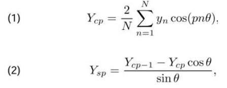
where Ycp and Ysp are the Fourier series coefficients, N is the samples per cycle, θ = 2π/N, yn is the sampled signal.
Distance Protection
Distance protection is suitable for distributed systems with DG because it only depends on the measured impedance between the relay and the protection zone. The general torque equation for distance protection is given by [27]:

where IR and VR are, respectively, the currents and voltages measured by the relay.
The relay will operate when ℛ(SopS*op)>0, where Sop is the operation torque and Spol is the polarization torque. All the distance characteristics can be designed through the change of the k1,…, k4 variables, as summarized in Table 1.
Table 1. k values for each distance characteristic.

The polarization voltage affects the mho dynamic behavior which depends on the system steady-state, and source impedance ratio [28]. The mho can be self, cross, positive sequence polarized, and many more types of polarization in order to operate properly. For three-phase faults or faults nearly the relay, the polarization voltage can be zero. For these situations, memory voltage is needed.
An example of memory polarization is the IIR filter proposed by [29]. For example, the polarization voltage of the relay A phase-ground unit is given by:
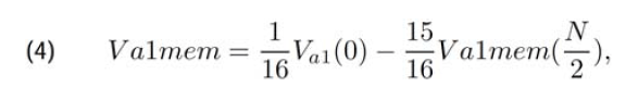
where Va1 is the positive symmetrical voltage and Va1mem is the memory positive symmetrical voltage.
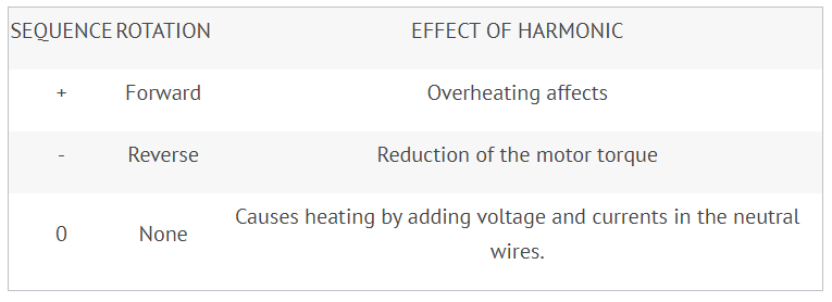
Similarly to the mho relay, the directional relay uses different polarization to operate. For example, the relay can use the zero and negative current as polarization. The choice of polarization influence in the general performance of the relay. For ground-phase units, the relay can use the zero and negative current as polarization, whereas the directional relay phase units only use the negative current.
Electric Network Modeling
The main characteristics of modeling the electrical system (Fig. 1)and the synchronous machine and control (Fig.2) used as a source of DG are presented in this section. The modeling and implementation of network components were simulated in the Smulink SimPowerSystem Matlab program [30].
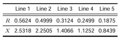
The test power system used presented in Fig. 1 [31] is a 132 kV transmission line Thevenin equivalent connected to a transformer 132/33 kV in delta/wye-ground. The 33 kV distribution system is composed by 5 equivalent RL branches, Table 2. This distribution system is connected to a synchronous generator of 30 MVA, DG, by a transformer 33/6.9 kV in delta/wye-ground.

Table 2. Line data, values in (Ω)
The load model dependent of the voltage used in the system [32,33] are represented by:

where P is the active power consumed by the load, P0 is the load active nominal power, Q is the reactive power consumed by the load, Q0 is the load reactive nominal power, V is the load nodal voltage, V0 is the load nominal voltage, np is an exponent that indicating the behavior of the load active power in relation to the nodal voltage variation, nq is an exponent that indicating the behavior of the load reactive power in relation to the nodal voltage variation. These values are presented in Table 3.
Table 3. Definition of electrical load types.

The synchronous generator excitation system connected in the distribution networks is usually made to control the terminal voltage. For synchronous generators connected to the distribution networks, generally, there are two forms of control that may be employed: constant voltage or reactive constant power [34]. A general scheme for the synchronous generator excitation system is depicted in Fig. 2, which consists in circuits of measuring and signals processing, a regulator system and an exciter system, where Efd is the voltage of exciter field.
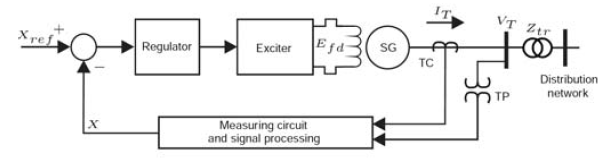
The model used for the synchronous generator excitation system is the IEEE type 1, was based on the model existent in the SimPowerSystem library [30].
Performance Assessment of the Distance Protection in Distribution System with DG
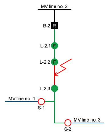
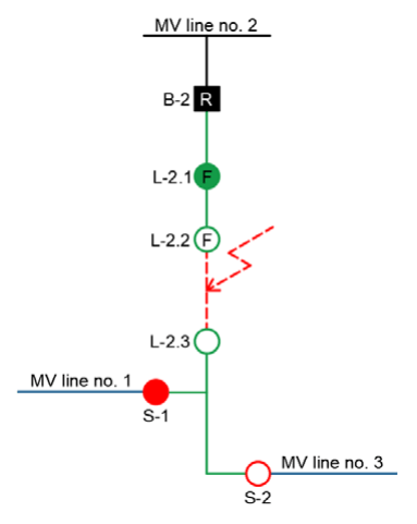
The power system diagrams with and without DG are depicted, respectively, in Fig. 3, and 4. In order to apply faults along the protected line, the line 1 is split in three RL branches, allowing faults with in 33% of the line length . Several faults in different locations of the power system, varying the ground resistance (Rg), phase resistance (Rab, Rbc, and Rac), and fault inception angle were simulated according to Table 4.


Table 4. Simulated Faults.

The fault simulations were simulated in various locations namely, in each bus of the system, and between each RL branch of the Line 1. The relay protection zone is defined to be between bus 2 and bus 3. In the protection zone, a total of 64 faults were simulated with and without DG according to Table 4. In outside of protection zone, a total of 48 faults were simulated without DG and a total of 64 faults were simulated with DG according to Table 4.
Fault Analysis
Several faults applied in the power system are analyzed according to the tripping time, and relay efficiency, comparing the results with and without DG in the system. Also, the distance protection capabilities of coordination are discussed.
The Fig. 5(a) and 5(b) depict an AG fault with and without DG simulated between L1−1 and L1−2 branch’s with a 0.0001 Ω impedance inside the protection zone. When the DG is presented, the trajectory impedance converges to a lower impedance value. This behavior can lead to a misoperation of distance protection, since the estimated impedance is near the operation distance characteristic.

Fig. 6(a) and 6(b) depict an AG fault with and without DG simulated in bus 4 with a 0.0001 Ω impedance located outside the protection zone. When the DG is presented, the trajectory impedance is influenced.
In Table 5, the mho and quadrilateral distance protection trips performed outside protection zone of the power system without DG are summarized. Only for ABC faults the distance protection relay has maloperations. These maloperations occurred in the equivalent power system bus 1.
Table 5. Mho and quadrilateral results outside protection zone without DG.


Table 6. Mho and quadrilateral results outside protection zone without DG.

In Table 6, the mho and quadrilateral distance protection trips performed outside protection zone of the power system with DG are summarized. Only for ABC faults, the distance protection relay has maloperations. These maloperations occurred in the equivalent power system bus 1. However, com- paring the Tables 5 and 6, the distance protection achieves the same results.
In Table 7, the mho and quadrilateral distance protection trips performed in the protection zone of the power system without DG are summarized. For AG faults, the mho and quadrilateral distance relay have tripped for all simulated situations. However, for the other fault types the mho and quadrilateral distance relays do not trip for the branch 2-4, but this is not a major problem because it is assured the coordination.
Table 7. Mho and quadrilateral results in protection zone without DG.

In Table 8, the mho and quadrilateral distance protection trips performed in the protection zone of the power system with DG are summarized. For AG faults, the mho and quadrilateral distance relay have tripped for all simulated situations. However, for the other fault types the mho and quadrilateral distance relay do not trip for the branch 2-4. Comparing the results between Tables 7 and 8, the mho and quadrilateral distance relay are not affected by the DG. In addition, the trip times are different with and without DG. In the presence of DG, the trip time is faster due to the measured impedance in the distribution system is lower. In conclusion, distance relays are good candidates to protect systems with DG penetration.
Table 8. Mho and quadrilateral results in protection zone with DG.

Conclusion
In this paper, distance protection applied in a distributed system with and without DG was presented. The distance mho and quadrilateral characteristics were used. The mho relay is composed with reactance and directional characteristics, and fault type supervision. Also, the quadrilateral re- lay is composed with two lateral blinders, reactance and directional characteristics, and fault type supervision. Several faults were simulated in the power systems varying the fault inception angle, location, fault type and fault resistance.
The distance protection presented good results and actuates properly for almost all the simulated faults. The distance protection performance was almost identical in the power system with and without DG in the simulated faults, demonstrating that can be a suitable solution to replace the overcurrent relays in distributed systems. However, the DG inclusion in the power system provoked, in faults situation, an impedance trajectory closest to the relay trip zone. In conclusion, the usage of distance protection can be a solution to solve the problems introduced by distributed generation.
REFERENCES
[1] S. M. Brahma, “Fault location in power distribution system with penetration of distributed generation,” IEEE Transactions on Power Delivery, vol. 26, no. 3, pp. 1545–1553, Jul. 2011.
[2] R. Chabanloo, H. Abyaneh, A. Agheli, and H. Rastegar, “Overcurrent relays coordination considering transient behaviour of fault current limiter and distributed generation in distribution power network,” IET Generation Transmission and Distribution, vol. 5, no. 9, pp. 903–911, Nov. 2011.
[3] P. Anderson, Power System Protection, ser. IEEE Press Power Engineering Series. McGraw-Hill, 1999. [Online]. Available: http://books.google.com.br/books?id=eP9qQgAACAAJ
[4] F. C. L. Trindade, K. V. do Nascimento, and J. C. M. Vieira, “Investigation on voltage sags caused by dg anti-islanding protection,” IEEE Transactions on Power Delivery, vol. 28, no. 2, pp. 972–980, Apr. 2013.
[5] J. Gomez, J. Vaschetti, C. Coyos, and C. Ibarlucea, “Distributed generation: impact on protections and power quality,” IEEE (Revista IEEE America Latina) Latin America Transactions, vol. 11, no. 1, pp. 460–465, Feb. 2013.
[6] P. D. Lezhniuk, I. O. Hunko, S. V. Kravchuk, P. Komada, K. Gromaszek, A. Mussabekova, N. Askarova, and A. Arman, “The influence of distributed power sources on active power loss in the microgrid,” Przeglad Elektrotechniczny, vol. 93, no. 03, pp. 107–112, March 2017.
[7] J. Gomez and M. Morcos, “Coordination of voltage sag and overcurrent protection in dg systems,” IEEE Transactions on Power Delivery, vol. 20, no. 1, pp. 214–218, Jan. 2005.
[8] F. Viawan and M. Reza, “The impact of synchronous distributed generation on voltage dip and overcurrent protection coordination,” in Future Power Systems, 2005 International Conference on, Nov 2005, pp. 6 pp.–6.
[9] S. Brahma, “Fault location in power distribution system with penetration of distributed generation,” Power Delivery, IEEE Transactions on, vol. 26, no. 3, pp. 1545–1553, July 2011.
[10] J. Silva, H. Funmilayo, and K. Butler-Purry, “Impact of distributed generation on the ieee 34 node radial test feeder with overcurrent protection,” in Power Symposium, 2007. NAPS ’07. 39th North American, Sept 2007, pp. 49–57.
[11] R. Chabanloo, H. Abyaneh, A. Agheli, and H. Rastegar, “Overcurrent relays coordination considering transient behaviour of fault current limiter and distributed generation in distribution power network,” Generation, Transmission Distribution, IET, vol.5, no. 9, pp. 903–911, September 2011.
[12] W. Elmore, Protective Relaying: Theory and Applications, ser. No Series. Marcel Dekker, 2004. [Online]. Available: http://books.google.com.br/books?id=1Jqhpd-rhoUC
[13] G. Ziegler, Numerical distance protection : principles and application / Gerhard Ziegler ; [editor, Siemens AG]. Munich : Publicis MCD, 1999, includes bibliographical references (p. 306-311) and index.
[14] REL300 Relay System, V2.71 ed., ABB Power T& D Company
Inc., 4 1996.
[15] D30 Line Distance Protection System Instruction Manual, GE Energy, 4 2012.
[16] SIPROTEC Distance Protection 7SA522, Siemens AG, 2 2011.
[17] C. Mason, The art and science of protective relaying, ser. General Electric series. Wiley, 1956. [Online]. Available: http://books.google.com.br/books?id=jedSAAAAMAAJ
[18] J. Suonan, J. Zhang, Z. Jiao, L. Yang, and G. Song, “Distance protection for hvdc transmission lines considering frequency dependent parameters,” Power Delivery, IEEE Transactions on, vol. 28, no. 2, pp. 723–732, April 2013.
[19] L. He, C.-C. Liu, A. Pitto, and D. Cirio, “Distance protection of ac grid with hvdc-connected offshore wind generators,” Power Delivery, IEEE Transactions on, vol. 29, no. 2, pp. 493–501, April 2014.
[20] F. Albasri, T. Sidhu, and R. Varma, “Performance comparison of distance protection schemes for shunt-facts compensated transmission lines,” Power Delivery, IEEE Transactions on, vol. 22, no. 4, pp. 2116–2125, Oct 2007.
[21] Z. Xu, S. Huang, L. Ran, J. Liu, Y. Qin, Q. Yang, and J. He, “A distance protection relay for a 1000-kv uhv transmission line,” Power Delivery, IEEE Transactions on, vol. 23, no. 4, pp. 1795–1804, Oct 2008.
[22] A. Hooshyar, M. Azzouz, and E. El-Saadany, “Distance protection of lines connected to induction generator-based wind farms during balanced faults,” Sustainable Energy, IEEE Transactions on, vol. 5, no. 4, pp. 1193–1203, Oct 2014.
[23] I. Chilvers, N. Jenkins, and C. P, “Distance relaying of 11 kv circuits to increase the installed capacity of distributed generation,” Generation, Transmission and Distribution, IEE Proceedings-, vol. 152, no. 1, pp. 40–46, Jan 2005.
[24] A. Sinclair, D. Finney, D. Martin, and P. Sharma, “Distance protection in distribution systems: How it assists with integrating distributed resources,” in Rural Electric Power Conference (REPC), 2013 IEEE, April 2013, pp. B3–1–B3–12.
[25] E. O. S. III and J. Roberts, ÂS¸ Distance Relay Element Design, ÂTˇ proceedings of the 47th Annual Texas A&M Conference for Protective Relay Engineers, College Station, TX, Apr. 1993. [Online]. Available: http://www.selinc.com/techpprs.htm
[26] D. G. Hart, D. Novosel, and R. A. Smith, “Modified cosine filters,” November 2000. [Online]. Available: http://www.freepatentsonline.com/6154687.html
[27] B. Kasztenny and D. Finney, “Fundamentals of distance protection,” in Protective Relay Engineers, 2008 61st Annual Conference for, april 2008, pp. 1 –34.
[28] J. Roberts, A. Guzman, and E. O. Schweitzer, Z=V/I Does Not Make a Distance Relay. 20th Annual Western Protective Relay Conference, Spokane, WA, Oct. 1993.
[29] E. O. Schweitzer III, Distance relay using a polarizing voltage, August 1992, no. 5140492. [Online]. Available: http://www.freepatentsonline.com/5140492.html
[30] Hydro-Québec, SimPowerSystemT M , User’s Guide (Second Generation. MathWorks disponível em: http://www.mathworks.com, 2013.
[31] D. Salles, W. Freitas, J. C. M. Vieira, and W. Xu, “Nondetection index of anti-islanding passive protection of synchronous distributed generators,” IEEE Transaction on Power Delivery, vol. 27, no. 3, pp. 1509 –1518, Jul. 2012.
[32] P. Kundur, Power System Stability and Control, 1st ed. McGraw-Hill Inc, 1994.
[33] IEEE-Standard, “Institute of electrial and electronics engineers standard: Ieee recommended practice for excitation system models for power system stability studies,” Standar Board, 2005.
[34] N. Jenkins, R. Allan, P. Crossley, D. Kirschen, and G. Strbac, Embedded Generation, first edition ed. London: IEEE. (IET Power and Energy Series 31), 2000.
Authors: João Tiago Laureiro Souza Campos, Po- tiguar University (UnP), Department of Electrical Engineer- ing, Lagoa Nova, 59.056-000, Natal – RN – Brazil, email: j.campos893@gmail.com.
Huilman Sanca Sanca, Federal University of Campina Grande (UFCG), Department of Electrical Engineering, Bodocongó, 58.429-900, Campina Grande – PB – Brazil, email: huilman.sanca@gmail.com.
Flávio Bezerra Costa, Federal University of Rio Grande do Norte (UFRN), School of Science and Technology, Lagoa Nova, 59.078-970, Natal – RN – Brazil., email: flaviocosta@ect.ufrn.br.
Benemar Alencar de Souza, Federal University of Camp- ina Grande (UFCG), Department of Electrical Engineering, Electrical Engineering and Informatics Centre, Bodocongó, 58.429-900, Campina Grande – PB – Brazil, email: benemar@dee.ufcg.edu.br.
Source & Publisher Item Identifier: PRZEGLĄD ELEKTROTECHNICZNY, ISSN 0033-2097, R. 94 NR 3/2018. doi:10.15199/48.2018.03.03